Page | i

THE AERODYNAMICS OF TRACTOR-TRAILER

COMMERCIAL VEHICLES

By

EDWARD COMER

A project submitted in partial fulfilment of the requirements for the degree of

B.E. in Energy Systems Engineering (Mechanical)

NATIONAL UNIVERSITY OF IRELAND, GALWAY

12th April 2013

Project Supervisor: Dr. John Eaton

Page | ii

Abstract

This report explains the reason why aerodynamics play such an important role in

the design of commercial trucks. It is established through the study of previous

papers based on the field of vehicle aerodynamics how the geometry of trucks

affects aerodynamics and fuel consumption. Improving the aerodynamics of

commercial tractor-trailer units involves the installation of drag reduction devices

in certain regions of the truck subject to the most drag force. In preparation for

the CFD (Computational Fluid Dynamics) study on model trucks a test case was

studied first. This study comprised of modelling a cube (a basic shape) for which

there is a known drag coefficient under given flow conditions. In this study a

similar result was achieved, and this was then used as a validation case for

subsequent truck models. Two drag reduction devices were modelled in this

report and their effects were analysed and reported accordingly. This report also

studied the interference gap between the tractor and trailer units. The gap width

was expressed non-dimensionally and its influence on the overall drag coefficient

was analysed via CFD simulations.

Page | iii

Acknowledgements

I would like to take this opportunity to thank everyone that has helped me over

the past eight months in the completion of this project. In particular I would like to

thank my lecturers for all their support and encouragement to me and my

classmates, not just with our projects but with our college lives in general. I would

also like to thank my fellow classmates for their help, especially over the last

year. It was great to have such considerate colleagues who were willing to help

me with those aspects of the project I found difficult. I would also like to thank my

parent’s as well for their help with this project. They were very supportive.

Most of all I would like to express my gratitude to my supervisor Dr. Eaton for his

knowledge and support over the year. He has given me a lot of valuable advice

for the project, which is much appreciated.

Page | iv

Statement of Originality

Mechanical and Biomedical Engineering, NUI Galway

Plagiarism Declaration

09071547 Comer Edward

Student Number Family Name Other Names

Project title: THE AERODYNAMICS OF TRACTOR-TRAILER COMMERCIAL

VEHICLES

I declare that:

I have read and understood both the NUI Galway Code of

Practice on Plagiarism and “Plagiarism – a guide for engineering

and I.T. students in NUI, Galway”.

I am the original author of all work included in this report, except

for material which has been fully and properly acknowledges

using a standard referencing method.

The material in this report has not been presented for assessment

in any other course in this university of elsewhere.

I have taken all reasonable care to ensure that no other person has

been able to copy any part of this report either in paper or

electronic form.

Signature Date

Page | v

Contents

Statement of Originality ................................................................................... iv

List of Figures ................................................................................................. vii

List of Tables ................................................................................................... ix

1. INTRODUCTION ............................................................................................. 1

1.1 Project Objectives .................................................................................. 1

1.2 An introduction to fluid mechanics .............................................................. 2

Properties of incompressible fluids ............................................................... 2

External flow phenomena ............................................................................. 3

1.3 Motivation ................................................................................................... 4

1.4 Fuel Consumption and Drag Reduction ...................................................... 5

Resistance to Motion .................................................................................... 5

Add-on Devices ............................................................................................ 8

Traditional methods of studying vehicle aerodynamics ................................. 9

2. BACKGROUND INFORMAION ON CFD ...................................................... 10

2.1 CFD Background ...................................................................................... 10

Pre-processing ........................................................................................... 10

Solving ........................................................................................................ 11

Post-processing .......................................................................................... 11

2.2 Flow regimes ............................................................................................ 12

Inviscid flow ................................................................................................ 12

Laminar flow ............................................................................................... 13

Turbulent flow ............................................................................................. 13

2.3 Boundary Conditions ................................................................................ 15

2.4 Ansys - Fluent .......................................................................................... 16

3. CONFIGURATIONS SIMULATED ................................................................. 17

3.1 The Cube study ........................................................................................ 17

Geometry Setup ......................................................................................... 18

Mesh setup ................................................................................................. 19

Problem setup ............................................................................................ 20

Re-meshing setup ...................................................................................... 22

Problem setup ............................................................................................ 24

3.2 Interference gap width study .................................................................... 24

Geometry Setup ......................................................................................... 26

Mesh Setup ................................................................................................ 26

Page | vi

Problem setup ............................................................................................ 27

3.3 Interference Gap Blocker Study ................................................................ 28

3.4 Deflector Design Study ............................................................................. 29

Design Method ........................................................................................... 30

Deflector Optimization ................................................................................ 30

3.5 Cross-wind study ...................................................................................... 34

Geometry Setup ......................................................................................... 35

Mesh setup ................................................................................................. 35

Problem setup ............................................................................................ 36

4. RESULTS AND DISCUSSION ...................................................................... 38

4.1 The Cube ................................................................................................. 38

4.2 Interference Gap Investigation.................................................................. 43

4.3 Interference Gap Blocker .......................................................................... 48

4.4 Deflector Investigation .............................................................................. 49

4.5 Crosswind Investigation............................................................................ 52

4.6 Limitations ................................................................................................ 59

4.7 Recommendations for future work ............................................................ 59

5. CONCLUSIONS ............................................................................................ 60

REFERENCES............................................................................................... 62

APPENDICES ................................................................................................ 63

Page | vii

List of Figures

Figure 1-1: The flow field around a commercial truck ........................................... 3

Figure 1-2: Influence of drag on fuel consumption of a 38 tonne truck [2] ............ 5

Figure 1-3 Rolling & drag resistance curves under still air and level road

conditions[x] ......................................................................................................... 6

Figure 1-4 Pressure and friction drag [4] .............................................................. 7

Figure 1-5 Breakdown of drag on a 38 tonne truck .............................................. 8

Figure 1-6 Base plate flaps .................................................................................. 9

Figure 3-1 Problem specification in Fluent ......................................................... 18

Figure 3-2 Geometry specification NOT TO SCALE .......................................... 18

Figure 3-3 Initial mesh specification ................................................................... 19

Figure 3-4 Problem setup in Ansys Fluent ......................................................... 21

Figure 3-5 Reference values used in the initial simulation .................................. 22

Figure 3-6 Comparison of the coarse grid (left) and the fine grid (right) ............. 24

Figure 3-7 Model truck showing the non-dimensional b/h ratio ........................... 25

Figure 3-8 Case 2 with the gap blocker installed ................................................ 29

Figure 3-9 Initial deflector design ....................................................................... 30

Figure 3-10 Deflector design 2 with a fillet radius of 300 mm ............................. 31

Figure 3-11 Deflector deign 3 with fillet radius of 500 mm .................................. 31

Figure 3-12 Datum truck with deflector 3 attached ............................................. 32

Figure 3-13 Deflector design 4 ........................................................................... 32

Figure 3-14 Datum truck with deflector 4 attached ............................................. 33

Figure 3-15 Deflector design 5 ........................................................................... 33

Figure 3-16 Mesh refinement of case 1 with deflector 5 ..................................... 34

Figure 3-17 Comparison of a truck in still air (a) and one with a cross-wind at

angle θ° ............................................................................................................. 35

Figure 3-18 Named Selection surfaces for velocity inlet (top) and pressure outlet

(bottom) ............................................................................................................. 36

Page | viii

Figure 4-1 Mesh, flow regime and upwind scheme comparison ......................... 38

Figure 4-2 Velocity distribution contours along the symmetry plane for the initial

enclosure (top) and for the enlarged enclosure (bottom) .................................... 40

Figure 4-3 Pressure distribution contours along the symmetry plane from the

initial enclosure (top) enlarged enclosure (bottom)............................................. 41

Figure 4-4 Pressure distribution contours along the cubes surfaces .................. 42

Figure 4-5 Pressure distribution contours along the front (left) and rear (right)

surfaces of the cube .......................................................................................... 42

Figure 4-6 Influence of the growing interference gap on drag ............................ 44

Figure 4-7Gap width vs b/h ratio using two more cases ..................................... 45

Figure 4-8 Pressure distribution contours on the front (a) and rear (b) surfaces of

the datum truck .................................................................................................. 47

Figure 4-9 Case 2. Drag coefficient comparison of the interference gap blocker 48

Figure 4-10 Drag coefficient vs varying gap width of the models with and without

the deflector ....................................................................................................... 49

Figure 4-11 Drag coefficients of each deflector on the datum case. ................... 50

Figure 4-12 Pressure contours along the truck in Case 1 with no deflector ........ 51

Figure 4-13 Pressure contours along the truck in Case 1 with deflector 3 .......... 51

Figure 4-14 Drag vs. yaw angle of different vehicle types .................................. 52

Figure 4-15 Calculated drag coefficient Vs. Yaw angle for the datum truck ........ 52

Figure 4-16 Cutting plane used in the simulations.............................................. 53

Figure 4-17 Velocity contours along A-A for the datum case at 30° crosswind ... 54

Figure 4-18 Pressure contours on the surface of the truck ................................. 54

Figure 4-19 Velocity vectors along A-A at 30° yaw angle for Case 5 (PLAN VIEW)

.......................................................................................................................... 55

Figure 4-20 Pressure coefficient contours along A-A at 30° yaw angle of Case 5

(PLAN VIEW) ..................................................................................................... 55

Figure 4-21 Velocity vectors along A-A at 30° yaw angle for Case 5 with the gap

blocker installed (PLAN VIEW) ................................................................ 56

Page | ix

Figure 4-22 Static pressure contours along A-A at 30° yaw angle of Case 5 with

the gap blocker installed (PLAN VIEW) .............................................................. 56

Figure 4-23 Pressure distribution along the left surface of the Case 5 truck with

the gap blocker installed .................................................................................... 57

Figure 4-24 Pressure distribution along the right surface of the Case 5 truck with

the gap blocker installed .................................................................................... 57

List of Tables

Table 1 Reynolds number parameters ............................................................... 20

Table 2 Grid sizes used for the comparison ....................................................... 23

Table 3 Documentation of the b/h ratio for each case ........................................ 25

Table 4 B.C. summarization of the problem ....................................................... 27

Table 5 x & y components of velocity required for each yaw angle .................... 37

Table 6 Mesh 1 drag coefficients for various turbulence models and upwind

schemes ............................................................................................................ 39

Table 7 Mesh 2 drag coefficients for various turbulence models and upwind

schemes ............................................................................................................ 39

Table 8 Mesh 3 drag coefficients for various turbulence models and upwind

schemes ............................................................................................................ 39

Table 9 Calculated force on the cube with the initial enclosure in the x-direction 40

Table 10 Breakdown of the drag coefficient for each case ................................. 46

Table 11 Breakdown of the drag coefficient for each case ................................. 46

Table 12 Force components on each surface of the datum truck ....................... 46

Table 13 Drag reduction of deflector 1 ............................................................... 49

Table 14 Drag coefficients of each deflector ...................................................... 50

Table 15 Documentation of the drag coefficient for each angle .......................... 53

Page | 1

1. INTRODUCTION

The external aerodynamics of road vehicles have a strong influence on tractive

resistance, fuel consumption and stability. This project will study the

aerodynamics of semi-trailer commercial trucks, where there is strong

aerodynamic interference between the tractor and trailer units, and much scope

remains for improvement.

1.1 Project Objectives

The objectives of this project are clearly stated as follows;

To summarize the reasons why aerodynamics and drag reduction is a

crucial aspect of commercial vehicle design.

To do a review of the current collection of drag reduction devices used by

the trucking industry.

To simulate with CFD the influence drag reduction devices have on the

overall drag coefficient of a particular model truck.

Page | 2

1.2 An introduction to fluid mechanics

In terms of road vehicles one of the most important physics at play is fluid

mechanics. Fluid mechanics is an enormous, well matured field of science so

only the most applicable aspects will be discussed in this report ie, the

fundamentals. The most applicable aspects of fluid mechanics relative to vehicle

motion include; the properties of incompressible fluids, external flow phenomena

and viscosity effects.

Properties of incompressible fluids

Density

Density is defined as a certain quantity of mass relative to its volume. The density

of fluids depends on the pressure and temperature it’s subject to. In general fluid

motion variations in density are critical, complicating all equations describing

motion. However with regards to the flow of air around a body, density only varies

at a Mach number greater than 0.3. This implies a very high velocity is required

for the flow to become compressible, so in terms of vehicle motion density can be

assumed constant, which simplifies matters greatly. The value of density used

throughout this report is;

Viscosity

Fluid viscosity is a more complicated property, defined as fluid resistance to

deformation. This ‘deformation’ is caused by an applied stress which more often

than not is shear stress. The cause of viscosity is due to friction at a molecular

level between particles and relates momentum flux to velocity gradient. For

Newtonian fluids there exists a linear relationship between momentum flux and

velocity gradient. The constant of proportionality is the dynamic viscosity , as

the equation below shows.

This equation is valid for a Newtonian flow parallel to a wall. The applied shear

stress is and the velocity gradient is du/dy. Since incompressible flow fields are

Page | 3

assumed through this report the viscosity is only dependant on temperature and

its value is taken constant as

External flow phenomena

In general there are two flow phenomena in fluids, internal and external. Internal

flow is concerned with motion inside a confined space like a pipe for instance.

This type of flow field doesn’t relate to vehicle motion as the passing air over a

vehicle isn’t confined. For this reason only external flow phenomena will be

discussed.

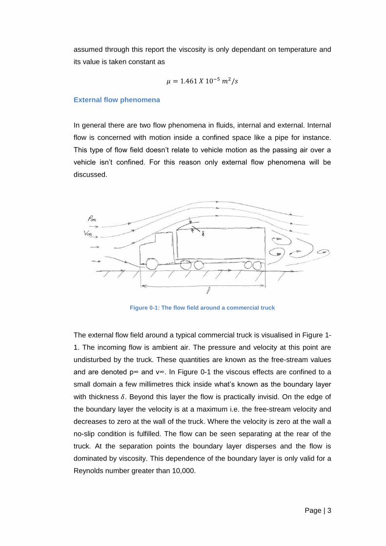
Figure 0-1: The flow field around a commercial truck

The external flow field around a typical commercial truck is visualised in Figure 1-

1. The incoming flow is ambient air. The pressure and velocity at this point are

undisturbed by the truck. These quantities are known as the free-stream values

and are denoted p∞ and v∞. In Figure 0-1 the viscous effects are confined to a

small domain a few millimetres thick inside what’s known as the boundary layer

with thickness . Beyond this layer the flow is practically invisid. On the edge of

the boundary layer the velocity is at a maximum i.e. the free-stream velocity and

decreases to zero at the wall of the truck. Where the velocity is zero at the wall a

no-slip condition is fulfilled. The flow can be seen separating at the rear of the

truck. At the separation points the boundary layer disperses and the flow is

dominated by viscosity. This dependence of the boundary layer is only valid for a

Reynolds number greater than 10,000.

Page | 4

1.3 Motivation

The past couple of decades have shown remarkable development in vehicle

aerodynamics and in particular commercial vehicle aerodynamics. There are two

primary reasons for this; advancement in CFD technology and soaring oil prices.

The fluctuating price of oil has encouraged trucking companies to invest in

aerodynamic improvements in their tractor-trailer units after it was established

aerodynamic efficiency corresponds to better fuel economy. Also, the increased

computing power over the years has made CFD simulations more common

place, and more accurate solutions have reduced the need for wind tunnel

testing.

Wind tunnel data is still the best information available for basing aerodynamic

analyses upon but such data is expensive to obtain. A much larger investment is

required as well as a longer experiment period. Wind tunnels contain blocking

effects, and a detailed description of the entire flow field cannot be acquired [1].

Numeric simulations can be run for a fraction of the price and decent results can

be achieved with a good methodology in CFD techniques (appropriately refined

meshes, appropriate boundary conditions, turbulence models, etc). CFD analysis

has a much shorter development cycle than wind tunnel investigations and good

reproducibility of results is long established. Another advantage of using CFD

over wind tunnel analysis is that the physical value at point in the flow field can be

drawn out and all parameter quantities are easy obtainable [1].

In 2003 the U.S. Department of Energy (DOE) conducted an investigation into the

freight transportation industry. According to this survey there are more than

2,200,000 commercial trucks operating on American highways. Over the course

of one year each truck covers 62,900 miles at 5.2 mpg (miles per gallon). This

amounts to approximately gallons of diesel per year. At currents diesel

prices ($3.6/gallon) this translates to an astronomical $90 billion dollars annual

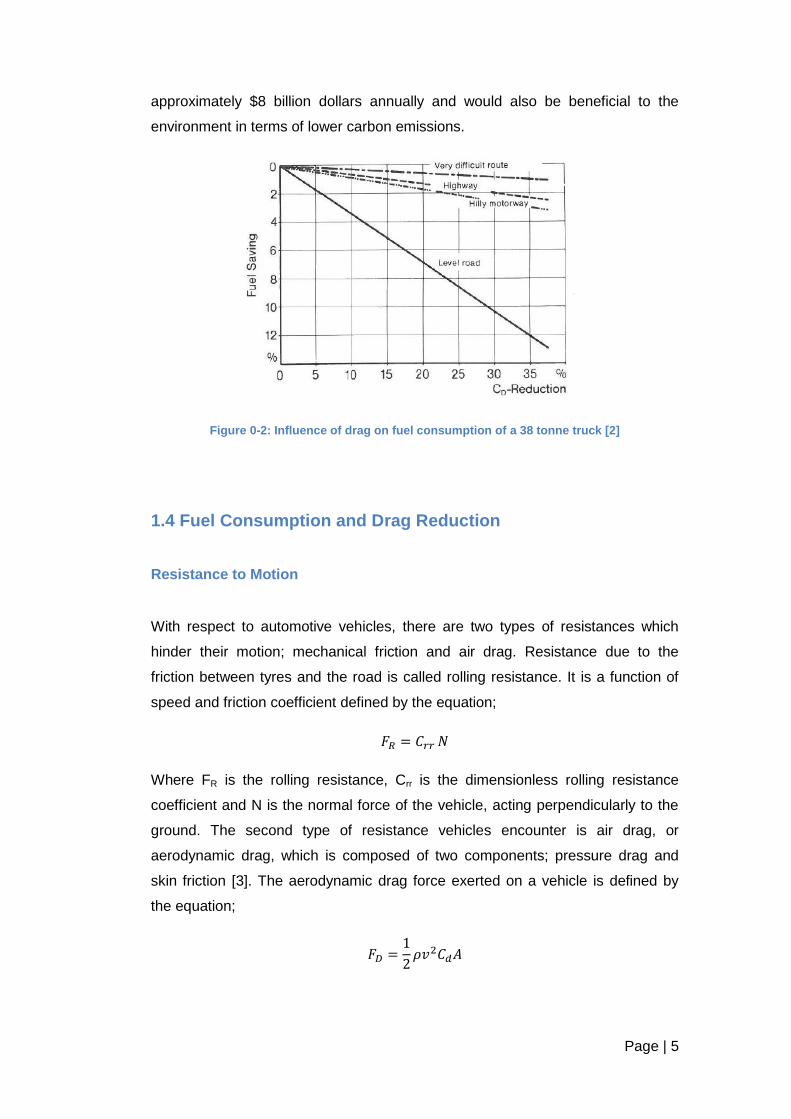
fuel cost [1]. Herein lays the motivation for improving truck aerodynamics. Figure

0-2 shows a graph comparing fuel economy to percentage drag reduction. It can

be seen that a roughly 28% decrease in drag corresponds to a 10% fuel saving.

Applying such a saving across the whole trucking sector would save

Page | 5

approximately $8 billion dollars annually and would also be beneficial to the

environment in terms of lower carbon emissions.

Figure 0-2: Influence of drag on fuel consumption of a 38 tonne truck [2]

1.4 Fuel Consumption and Drag Reduction

Resistance to Motion

With respect to automotive vehicles, there are two types of resistances which

hinder their motion; mechanical friction and air drag. Resistance due to the

friction between tyres and the road is called rolling resistance. It is a function of

speed and friction coefficient defined by the equation;

Where FR is the rolling resistance, Crr is the dimensionless rolling resistance

coefficient and N is the normal force of the vehicle, acting perpendicularly to the

ground. The second type of resistance vehicles encounter is air drag, or

aerodynamic drag, which is composed of two components; pressure drag and

skin friction [3]. The aerodynamic drag force exerted on a vehicle is defined by

the equation;

Page | 6

Where A is the projected area of the vehicle and CD is the drag coefficient of the

vehicle. Both rolling resistance and air drag have a negative effect on fuel

consumption, but their contributions vary at different speeds. This report is only

going to examine the effects of aerodynamic drag.

As vehicle speed increases the influence of drag also increases parabolically

(assuming a constant flow pattern) as shown in Figure 0-3. The power consumed

by a vehicle is proportional to the cube of its speed. Rolling resistance increases

linearly and at low speeds it is more dominant but an intersection point can be

seen at roughly 56 mph. This point marks the growing influence of aerodynamic

drag. Speeds beyond this point indicate drag is more resistant to vehicle motion.

This is because drag increases with the square of velocity, as already shown.

The power required for a 38 tonne truck to overcome aerodynamic drag at 37mph

is 25kW. By making aerodynamic improvements to the truck this required power

can be brought down. The quadratically increasing drag force beyond this

intersection point has encouraged places such as the United States to set the

speed limit of class 8 (38 tonne) trucks to 56mph in an effort to increase fuel

economy.

Figure 0-3 Rolling & drag resistance curves under still air and level road conditions[x]

Page | 7

Aerodynamic drag, as previously stated, comprises of two components; pressure

drag and skin friction. The magnitude of each component varies depending on

the geometric shape of the body subject to a flow and the characteristics of the

flow itself. For flow over slim bodies where the overall surface area is small the

drag force is dominated by friction drag. However for large, bluff bodies with

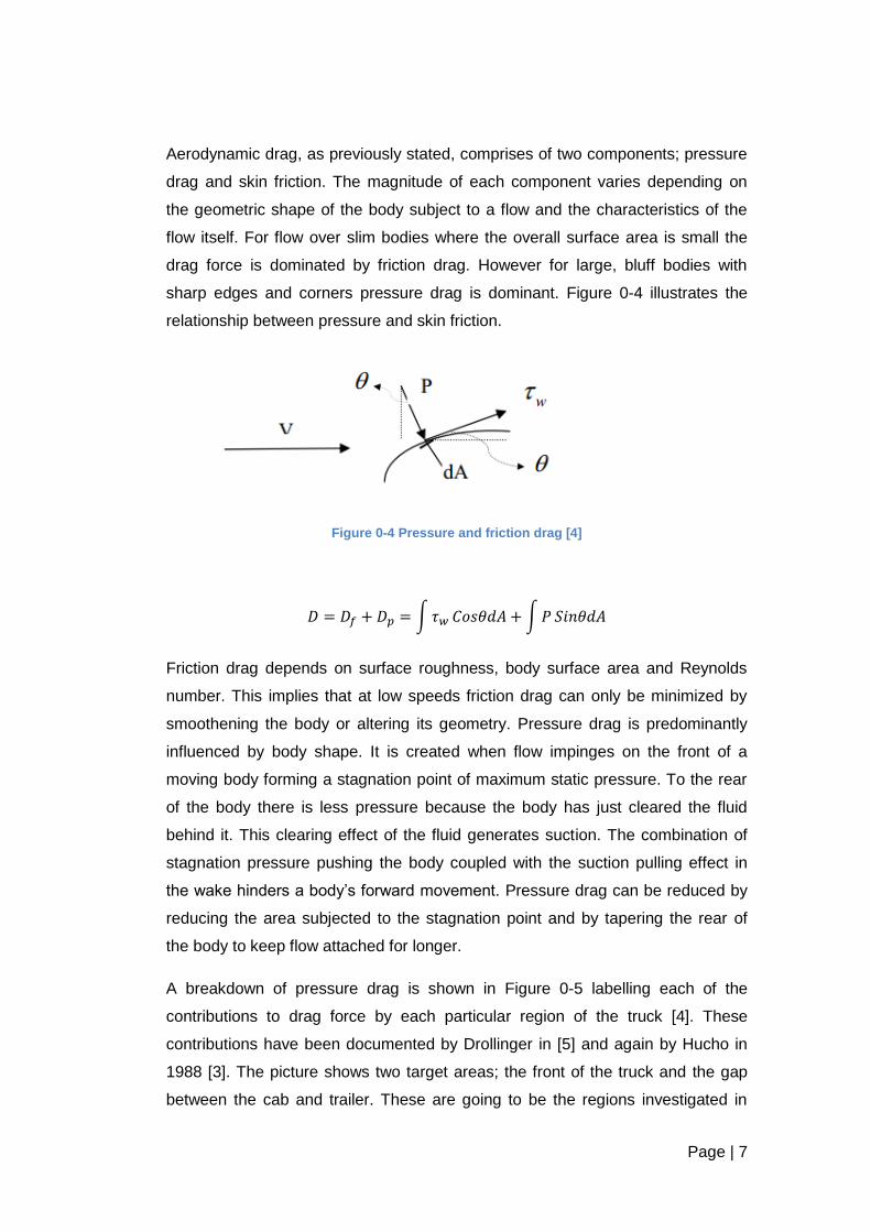
sharp edges and corners pressure drag is dominant. Figure 0-4 illustrates the

relationship between pressure and skin friction.

Figure 0-4 Pressure and friction drag [4]

∫ ∫

Friction drag depends on surface roughness, body surface area and Reynolds

number. This implies that at low speeds friction drag can only be minimized by

smoothening the body or altering its geometry. Pressure drag is predominantly

influenced by body shape. It is created when flow impinges on the front of a

moving body forming a stagnation point of maximum static pressure. To the rear

of the body there is less pressure because the body has just cleared the fluid

behind it. This clearing effect of the fluid generates suction. The combination of

stagnation pressure pushing the body coupled with the suction pulling effect in

the wake hinders a body’s forward movement. Pressure drag can be reduced by

reducing the area subjected to the stagnation point and by tapering the rear of

the body to keep flow attached for longer.

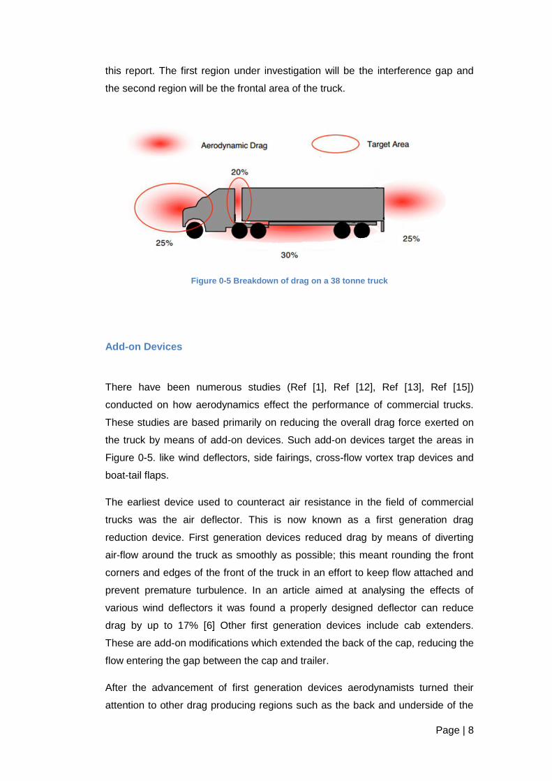
A breakdown of pressure drag is shown in Figure 0-5 labelling each of the

contributions to drag force by each particular region of the truck [4]. These

contributions have been documented by Drollinger in [5] and again by Hucho in

1988 [3]. The picture shows two target areas; the front of the truck and the gap

between the cab and trailer. These are going to be the regions investigated in

Page | 8

this report. The first region under investigation will be the interference gap and

the second region will be the frontal area of the truck.

Figure 0-5 Breakdown of drag on a 38 tonne truck

Add-on Devices

There have been numerous studies (Ref [1], Ref [12], Ref [13], Ref [15])

conducted on how aerodynamics effect the performance of commercial trucks.

These studies are based primarily on reducing the overall drag force exerted on

the truck by means of add-on devices. Such add-on devices target the areas in

Figure 0-5. like wind deflectors, side fairings, cross-flow vortex trap devices and

boat-tail flaps.

The earliest device used to counteract air resistance in the field of commercial

trucks was the air deflector. This is now known as a first generation drag

reduction device. First generation devices reduced drag by means of diverting

air-flow around the truck as smoothly as possible; this meant rounding the front

corners and edges of the front of the truck in an effort to keep flow attached and

prevent premature turbulence. In an article aimed at analysing the effects of

various wind deflectors it was found a properly designed deflector can reduce

drag by up to 17% [6] Other first generation devices include cab extenders.

These are add-on modifications which extended the back of the cap, reducing the

flow entering the gap between the cap and trailer.

After the advancement of first generation devices aerodynamists turned their

attention to other drag producing regions such as the back and underside of the

Page | 9

truck. Second generation devices have been developed for these areas over the

past twenty years. Boat-tail flaps, also known as base plate flaps generally

comprise of four plates attached to the four edges of the trailer rear. They

protrude behind the truck at an angle in an effort to keep flow attached for longer,

increasing the wake pressure. A depiction of base tail flaps shown in Figure 0-6.

Figure 0-6 Base plate flaps

The main methods of studying the effectiveness of such drag reduction devices

has been experimentally and computationally via wind tunnel tests or CFD

programs. Drag reduction investigations test add-on devices by equipping them

to a scale model of the truck or an actual full scale model under similar Reynolds

number flows. Modelling full scale trucks generally involves using a simplified

geometry because of the complexity of the vehicle. This report adopts a similar

approach of modelling simple shapes.

Traditional methods of studying vehicle aerodynamics

The traditional methods used for analysing the flow-field over an automobile are

wind tunnel tests and road tests. As already stated, full scale model experiments

are expensive to perform in wind tunnels because of both the tunnels initial

capital cost and its operational cost. Scale models maybe used as a cheaper

means of testing but any results obtained are open to debate due to the potential

inaccuracy of estimating flow parameters like the Reynolds number, surface

roughness and surface detail of the body [3]. Road tests represent the most

realistic means of analysing vehicle aerodynamics due to the use of real world

environmental conditions. However road tests, as one may imagine are very

difficult to perform especially for commercial vehicles like tractor-trailer units

given the cruising speeds of the vehicle. The constantly changing environment

also makes results difficult to replicate. These downsides of wind tunnel and road

tests which have encouraged the growth of CFD as a predictive tool for the

automotive industry.

Page | 10

2. BACKGROUND INFORMAION ON CFD

2.1 CFD Background

Computational Fluid Dynamics solves and analyses fluid based physics problems

using algorithms and numerical techniques performed on a computer. The

exponential growth of technology over the past twenty years has given rise to

powerful computers capable of performing these numerical methods with ease.

Computers solve fluid problems by analysing the interactions of liquids or gases

with surfaces defined by boundary conditions.

The basis for CFD simulations are the underlying mathematics which describe

fluid motion, most notably the ‘Navier-Stokes equations’; a set of non-linear

partial differential equations which can describe any single state fluid flow. These

equations in their full form, without any simplification are known as ‘the full

Navier-Stokes equations’. They can be broken down into simpler equations

depending on the fluid flow application for an easier approach to solving a

problem. This is discussed in Chapter 2.3.

CFD codes have sophisticated Graphical User Interfaces (GUI’s) to guide the

user around its immense processing power. Any commercial CFD package will

have three elements; pre-processing, solving and post processing.

Pre-processing

This is the first stage of the CFD process. It involves creating the fluid geometry

and initialising the problem. There are three parts to the pre-processing stage;

geometry setup, mesh setup and problem setup. Geometry setup can be done

with some CFD packages but it’s common to define the geometry in a separate

3D CAD package and import it into the meshing application within the CFD

program in the form of a STEP or IGEES file (program neutral files).

Once the total flow domain is defined it is broken down further into non-

overlapping sub-domains called the ‘computational grid’ or ‘mesh’. Each of the

individual elements or cells within the grid will have values for fluid properties like

velocity, pressure, temperature, etc. The code the program uses will solve the

governing equations for each property within the elements. This implies that the

more elements contained in the grid the more accurate the solution [7]. There is a

Page | 11

trade off to be made here between solution accuracy and computational cost.

The computer has to solve equations for each element so having a very fine

mesh means it has to work longer to get a solution. Complex meshing

applications within CFD codes allow for very particular space discretization,

meaning elements can be spaced throughout the grid in intelligent regions. This

process of placing elements in areas of interest is called ‘mesh optimization’.

Because programs have a maximum amount of elements associated with them

mesh optimization is very important. It is better to have a denser mesh around

regions where large variations occur from point to point and a coarse mesh

around regions with relatively little change [7]. Once the mesh is created the

problem boundary conditions and flow properties (B.C.’s) are specified, then

solving can begin. Flow regimes and B.C.’s are another big part of CFD analysis

and are discussed in detail in Chapter 2.3.

Solving

CFD codes operate on one of three numerical solution techniques; Finite

Difference Method (FDM), Finite Element Method (FEM) or Spectral Method.

Most codes use a variation of the FDM called the Finite Volume Method (FVM)

because it’s suited to representing and evaluating partial differential equations

(e.g. Navier-Stokes equations) as a system of algebraic equations. There is a

systematic approach to the FVM, which is as follows; integration of the governing

equations over the finite control volume of the domain, conversion of the integral

equations into algebraic ones and then solving them via an iterative method [7].

Post-processing

Once a solution to a problem has been obtained analysis can began. The aim of

post-processing is to identify and present results in the best manner possible.

The main aspect of results presentation are visualisation plots, i.e. contour plots,

vector plots, streamline plots of flow variables. Fantastic images and simulation

videos can be produced from top CFD programs.

Page | 12

2.2 Flow regimes

Within CFD simulations the specified flow regime is of high importance. This is

because the type of flow simulated has consequences on the governing

equations the computer program solves, which of course directly influences the

solution. Within any well established CFD code there are three flow regimes,

listed below.

Inviscid flow

Laminar flow

Turbulent flow

Inviscid flow

Inviscid flow is by far the easiest to model. It represents an ideal fluid meaning

there’s no viscosity in the flow field. Not having a viscosity term reduces the

Navier-Stokes equations to the Euler equations as shown in equations 1 and 2,

which any CFD code can solve simply with potential theory. However inviscid

flow is an impossible phenomenon as all flows have some viscosity, no matter

how small. It can be applied to very high Reynolds number flow fields where the

inertial forces far outweigh the viscous. For example inviscid models are used

routinely in aircraft design. Inviscid flows agree strongly with low viscosity flows

everywhere except close to the boundary of the fluid, which plays a very

significant role.

Page | 13

Laminar flow

Laminar flow is the next step up from inviscid flow. It’s modelled by the unsteady

Navier-Stokes equations in CFD programmes. Laminar flow can be described by

a one equation model. Obviously though laminar flow simulation is only valid for

low Reynolds numbers. It’s not particularly valid when analysing the

aerodynamics of commercial trucks. Never the less, all three models will be

analysed on the test case specimen, the cube. Under the test case investigation

the effects of various parameters will be modelled. The flow regime will be one of

these.

Turbulent flow

Turbulent flow is without question the most important flow regime examined by

this report. Turbulent flow fields have large Reynolds numbers and are more

suited to the flows around trucks driving at cruise speed than inviscid or laminar

flows. In CFD analysis though, there is no simple turbulence model which fits all.

A model will be chosen by matching the physics of the application with the

models available in the CFD package. Engineering judgment will be used to

predict what flow features are likely to occur in each particular case and which

features will have the most impact on the information sought.

Turbulence models are important because not every scale of motion can be

captured. To do this the size of computers required and the computational cost

would be enormous. Coupled with this, CFD practitioners rather a steady-state

solution with all fluctuations averaged out, rather than a time accurate one. With

this in mind only steady-state models will be used throughout the report.

Turbulence models are broken down and characterised by which governing

equations they solve, the Reynolds Averaged Navier-Stokes equations, (RANS),

or Large Eddy Simulation equations, (LES). This report is not going to go into

detail on either type of equations but for all CFD analysis conducted turbulence

models will solve the RANS because this is what’s used for most production

applications.

Page | 14

Furthermore models which solve the RANS are broken down into how many

extra equations they solve. There are three main categories, zero-equation

models, one-equation models and two-equation models. There are higher

equation models but they will not be discussed. Zero-equation models are by far

the simplest because they don’t require the solution to an extra transport

equation to compute the contribution of turbulence. Zero-equation models, also

known as algebraic models use only the flow variables and as such cannot

predict turbulence history like the convection and diffusion of turbulent kinetic

energy. Because of this, algebraic models are not very good for general cases

and won’t be discussed further in this report.

The next step up from algebraic models are one-equation models. As expected

one-equation models solve one extra equation, usually the turbulent kinetic

energy, for a quantity used to obtain the turbulent viscosity. Common one-

equation models are the Spalart-Allmaras and Goldberg models.

Two-equation models are the most common turbulence models used in

production. They solve two extra transport equations to determine the

contributions of turbulence to the mean flow. They’re able to determine history

effects of turbulence energy like its diffusion and convection, which can have big

effects on the overall solution to a problem. Since two-equation models give the

best trade off between accuracy and computational cost much research has gone

into developing them. Because of this there is a staggering amount of variations

so only the two used most frequently in industry will be discussed. These are the

k-epsilon model and the k-omega model.

The two extra transported variables in k-epsilon models, are of course, k and

epsilon. The former being the turbulent kinetic energy, the latter being the

turbulence dissipation rate. Epsilon determines the scale of turbulence, whereas

k determines its energy. K-epsilon models have been proven to be very useful for

cases involving free shear layers and small pressure gradients.

The k-omega model is very similar to the k-epsilon model; the difference being

omega is a measure of specific dissipation. K-omega models are proven to be

more accurate than k-epsilon models for simulating flows with adverse pressure

gradients and separation. However k-omega models have the downside of

Page | 15

producing large turbulence levels in regions where there’s a big amplitude of

normal strain, like stagnation points and domains of high acceleration.

2.3 Boundary Conditions

When performing CFD analysis one of the most important factors dictating results

are the boundary conditions (B.C’s) imposed on the surfaces and interfaces

within the domain. It is critical correct B.C’s are used with the problem to get

accurate results. The standard method of imposing B.C.’s in CFD programs is by

creating ‘Named Selections’ (a collection of surfaces) and putting a condition on

them. The B.C.’s used in this project are ‘walls’ ‘symmetries’ ‘inlets’ and ‘outlets’

When analysing the flow of air past a truck within an enclosure the front face of

the enclosure would be defined as the fluid ‘inlet’, the back face of the enclosure

would be defined as the fluid ‘outlet’ The surfaces of the truck would be ‘walls’’

the bottom surface of the enclosure, the road would also be defined as a ‘wall’.

The top and sides of the enclosure would be ‘symmetries’.

The ‘wall’ condition imposed on the road and truck would be a no-slip condition.

This implies the velocity is zero along the surface. A no-slip condition is the most

accurate way of representing a wall which is stationary relative to the fluid

passing it. In reality a moving fluid in contact with a solid body cannot have

velocity relative to the body. The fluid velocity increases linearly away from the

wall until it reaches the free-stream velocity. This no-slip condition will be used on

all the surfaces of the truck.

Unlike the surfaces of the truck the road is not defined as a stationary wall. This

is because for simulation purposes only the truck is moving, which means both

the air and road are moving relative to it. Because of this a ‘moving wall’ will be

used for the road. The velocity of the road will be that of the air velocity. The

movement of the road and air would be the same as if the truck was moving and

the road and air were stationary. It is the principle of relativity which allows one to

reverse these ‘moving’ and ‘stationary’ conditions.

An ‘inlet’ B.C. in CFD specifies that it is on that surface (s) that the fluid is to enter

the domain. Generally speaking when an ‘inlet’ condition is applied the velocity

there is usually known, otherwise the problem will have to be defined via another

Page | 16

B.C. Velocity at the inlet can be specified in numerous ways, the default is

‘normal to boundary’. This can be changed if the fluid isn’t entering the domain

perpendicular to the inlet surface. Cartesian or cylindrical co-ordinates can be

specified instead.

The surfaces where the fluid is exiting the domain can be defined as an ‘outlet’

Pressure at the outlet can be specified to constrain the problem. For most

applications static pressure will be constant over the outlet surface (s). However,

there is an option to specify a radial equilibrium distribution if the pressure is

varying along the outlet e.g. for strongly swirling flows.

Symmetry boundary conditions can be used in fluid domains where the geometry

on either side of a plane is identical. The use of symmetry in CFD is of great

benefit. It reduces overall computation time and allows more elements to be used

in the domain.

2.4 Ansys - Fluent

The CFD software chosen for this project was Ansys-Fluent version 14. This

decision was made because it is the best package the National University of

Ireland Galway has student licenses for. Fluent is a powerful CFD tool which will

help in analysing the aerodynamic problems in this project. Fluent has all of the

aforementioned traits of any top spec code; geometry modeller, meshing

application, pre-processor, solver and post-processor. While the geometry

modeller in Ansys is very good, all of the 3D models used in the project were

generated in Autodesk Inventor because of the author’s proficiency in Inventor.

Ansys has a very interactive GUI and a new feature in the current release is

Ansys Workbench. Workbench allows the user to incorporate different elements

of a problem, like geometry or meshes into different problems. This enables the

user to drag and drop different aspects of a project into each other. Appendix L is

a picture of the interface of Ansys Workbench. It shows the entire collection of

components used within the project. Each box represents one particular

geometry or operating condition of a model.

Page | 17

3. CONFIGURATIONS SIMULATED

Upon starting off analysing a given flow problem in Fluent the user is faced with

three initial inputs; geometry, meshing and problem setup. After defining each

input the problem can be solved and then brought into a post processor to

visualise the results.

The methodology for the CFD analysis conducted is defined in this section of the

report for each of the following investigations;

1. The Cube

2. Interference gap width

3. Interference gap blocker

4. Deflector

5. Crosswind

3.1 The Cube study

The purpose of studying such an elementary shape in a project regarding vehicle

aerodynamics is mainly to get a feel for the software, but also to establish a

validation case for future truck models. According to results documented by

Frank M. White in ‘Fluid Mechanics’ edition 5, the coeffecient of drag of a cube

immersed in a free stream flow field is 1.07 for flows with a Reynolds number of

10,000 or greater [8]. The flow in this instance is perpendicular to a face of the

cube. If a similar drag coeffecient can be replicated it would be a good indication

that correct CFD techniques are been deployed and a good indication that results

obtained for subsequent truck models are reasonably accurate. This first case,

the cube, will also be referred to as the test case throughout the report. It is going

to be vigourously analysed and tested. A secondary purpose of analysing this

case in such detail is to establish what influence each of the parameters within

the program have on the overall results. Knowledge of such influence on the test

case can then be applied to subsequent cases.

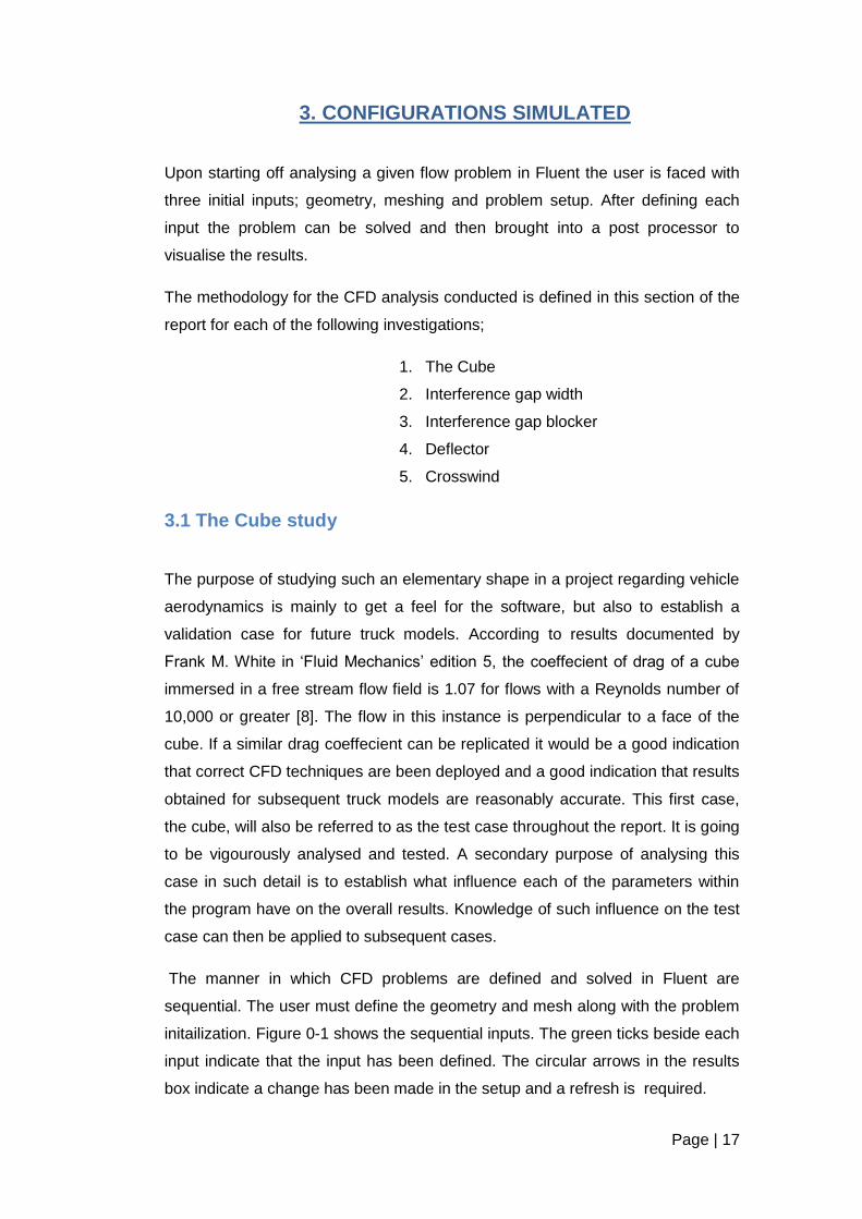
The manner in which CFD problems are defined and solved in Fluent are

sequential. The user must define the geometry and mesh along with the problem

initailization. Figure 0-1 shows the sequential inputs. The green ticks beside each

input indicate that the input has been defined. The circular arrows in the results

box indicate a change has been made in the setup and a refresh is required.

Page | 18

Figure 0-1 Problem specification in Fluent

Geometry Setup

For this case the flow of air over a cube is being studied. A control volume for this

air is required to analyse the flow but it’s not clear how big it has to be to

accurately analyse it. When sizing the control volume one doesn’t want to design

it too big because this will increase the elements within the domain and also the

computing time. With this in mind an initial enclosure was designed. Analysis was

performed using it and results are documented in Chapter 4.

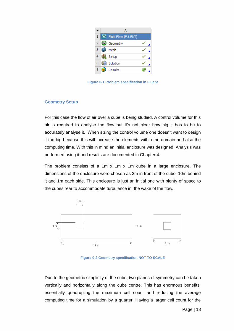
The problem consists of a 1m x 1m x 1m cube in a large enclosure. The

dimensions of the enclosure were chosen as 3m in front of the cube, 10m behind

it and 1m each side. This enclosure is just an initial one with plenty of space to

the cubes rear to accommodate turbulence in the wake of the flow.

Figure 0-2 Geometry specification NOT TO SCALE

Due to the geometric simplicity of the cube, two planes of symmetry can be taken

vertically and horizontally along the cube centre. This has enormous benefits,

essentially quadrupling the maximum cell count and reducing the average

computing time for a simulation by a quarter. Having a larger cell count for the

Page | 19

case will allow a better mesh convergence study. Once the enclosure was

created the program recognised two bodies; the cube and the enclosure itself.

Only the enclosure body was needed so a ‘Boolean’ operation was performed on

the geometry to subtract from the cube from the enclosure. Once this Boolean

was generated only the enclosure remained; this is the body of air used in the

analysis.

Mesh setup

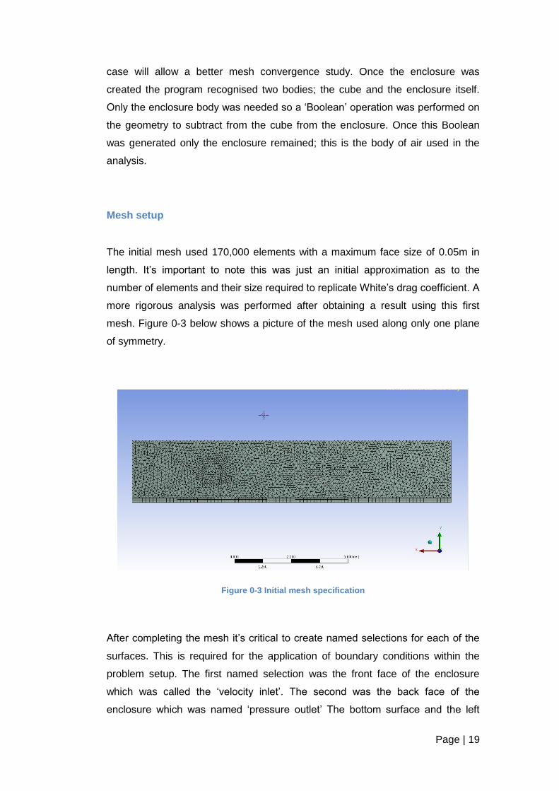
The initial mesh used 170,000 elements with a maximum face size of 0.05m in

length. It’s important to note this was just an initial approximation as to the

number of elements and their size required to replicate White’s drag coefficient. A

more rigorous analysis was performed after obtaining a result using this first

mesh. Figure 0-3 below shows a picture of the mesh used along only one plane

of symmetry.

Figure 0-3 Initial mesh specification

After completing the mesh it’s critical to create named selections for each of the

surfaces. This is required for the application of boundary conditions within the

problem setup. The first named selection was the front face of the enclosure

which was called the ‘velocity inlet’. The second was the back face of the

enclosure which was named ‘pressure outlet’ The bottom surface and the left

Page | 20

surface of the enclosure were called ‘symmetry’s’ because of the two symmetry

planes used in the creation of the model. The right surface and top surface of the

enclosure were named ‘symmetry right’ and ‘symmetry top’ respectively’ The four

visible faces of the cube were grouped together as one named selection called

‘cube’.

Problem setup

The problem was constrained to two important boundary conditions; an airflow

Reynolds number of 10,000 or above and a free-stream flow condition. Free-

stream flow means the cube won’t be affected by boundary layer growth from

other surfaces. The Reynolds number is the ratio of inertial force to viscous force

defined as;

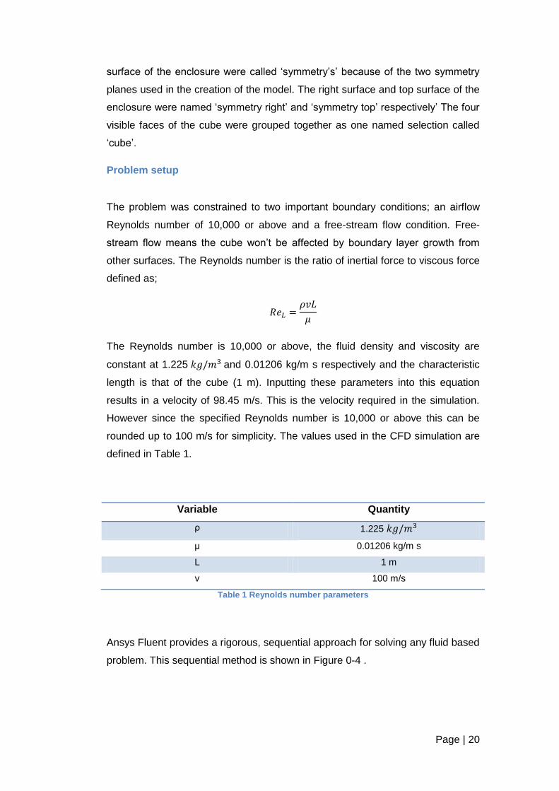
The Reynolds number is 10,000 or above, the fluid density and viscosity are

constant at 1.225 and 0.01206 kg/m s respectively and the characteristic

length is that of the cube (1 m). Inputting these parameters into this equation

results in a velocity of 98.45 m/s. This is the velocity required in the simulation.

However since the specified Reynolds number is 10,000 or above this can be

rounded up to 100 m/s for simplicity. The values used in the CFD simulation are

defined in Table 1.

Variable Quantity

ρ 1.225

μ 0.01206 kg/m s

L 1 m

v 100 m/s

Table 1 Reynolds number parameters

Ansys Fluent provides a rigorous, sequential approach for solving any fluid based

problem. This sequential method is shown in Figure 0-4 .

Page | 21

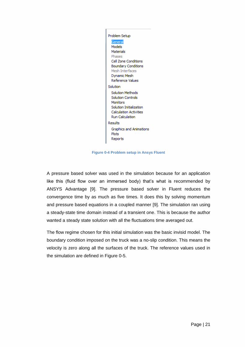
Figure 0-4 Problem setup in Ansys Fluent

A pressure based solver was used in the simulation because for an application

like this (fluid flow over an immersed body) that’s what is recommended by

ANSYS Advantage [9]. The pressure based solver in Fluent reduces the

convergence time by as much as five times. It does this by solving momentum

and pressure based equations in a coupled manner [9]. The simulation ran using

a steady-state time domain instead of a transient one. This is because the author

wanted a steady state solution with all the fluctuations time averaged out.

The flow regime chosen for this initial simulation was the basic invisid model. The

boundary condition imposed on the truck was a no-slip condition. This means the

velocity is zero along all the surfaces of the truck. The reference values used in

the simulation are defined in Figure 0-5.

Page | 22

Figure 0-5 Reference values used in the initial simulation

As can be seen from Figure 0-5. a reference area of was chosen. This is

because the two symmetry planes used quarters the area required for the

simulation. For this simulation the solution methods and controls were untouched,

left as the default settings.

After specifying the reference values a monitor for drag force was created. The

drag on the cube is the only drag force required so this was specified by choosing

‘cube’ under the named selections. The direction was also specified as the

negative x-direction (-1,0,0). This is the direction opposed to the front face of the

cube. A hybrid initialization was chosen over the standard initialization because it

efficiently initializes the solution based purely on simulation setup [9] meaning the

user doesn’t have to provide additional inputs. Once the solution was initialized a

request of 300 iterations was made and the program calculated the solution. The

results for this simulation are documented in Chapter 4.1.

Re-meshing setup

Based on the results from the initial enclosure it appears a better mesh is

required so a small mesh convergence study was undertaken. A proper mesh

convergence study cannot properly be undertaken because the maximum grid

Page | 23

size is too small. So this mesh convergence study is really more of a mesh

comparison.

For the study three grid sizes were analysed; a coarse mesh, a medium mesh

and a fine mesh, documented in Table 2. The course mesh used was just the

initial mesh Fluent creates around a body of air. There is no refinement.

Mesh Element size

Coarse mesh: 21,283 elements

Medium mesh: 104,898 elements

Fine mesh: 490,480 elements

Table 2 Grid sizes used for the comparison

The medium mesh contains roughly 105,000 elements. The main difference

between this mesh and the coarse one is the element sizing. The size of an

elements face in this mesh was limited to a maximum 0.6m. This increased the

cell count from 21,000 to 105,000 elements.

For the fine mesh, advanced sizing functions were used in Fluents meshing

application. The advanced sizing function chosen was proximity and curvature.

This yields a smaller element size the closer the mesh is to the edges of the

cube. A medium relevance centre was chosen which induced a 20% growth rate

for the elements. A slow element transition rate was specified in this case

because it’s more suited to CFD analysis than a fast transition due to the fact it

fills the volume with elements more smoothly and efficiently. The minimum

element size was specified as 0.01m even though the program probably won’t

create elements this small. The minimum size here is not that important. The

maximum element size is however, and it was set to 0.12m. With these settings

in place the grid size increased to 490,480 elements. A comparison can be seen

of the coarse grid and the fine grid in Figure 0-6

Page | 24

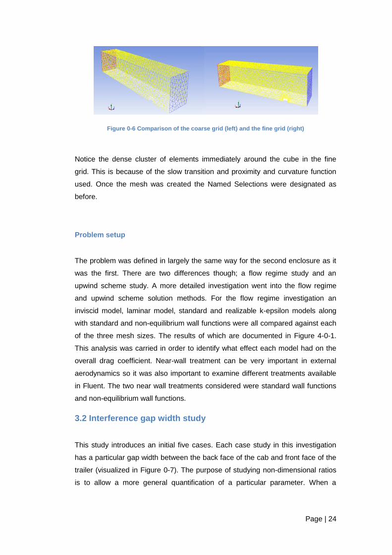
Figure 0-6 Comparison of the coarse grid (left) and the fine grid (right)

Notice the dense cluster of elements immediately around the cube in the fine

grid. This is because of the slow transition and proximity and curvature function

used. Once the mesh was created the Named Selections were designated as

before.

Problem setup

The problem was defined in largely the same way for the second enclosure as it

was the first. There are two differences though; a flow regime study and an

upwind scheme study. A more detailed investigation went into the flow regime

and upwind scheme solution methods. For the flow regime investigation an

inviscid model, laminar model, standard and realizable k-epsilon models along

with standard and non-equilibrium wall functions were all compared against each

of the three mesh sizes. The results of which are documented in Figure 4-0-1.

This analysis was carried in order to identify what effect each model had on the

overall drag coefficient. Near-wall treatment can be very important in external

aerodynamics so it was also important to examine different treatments available

in Fluent. The two near wall treatments considered were standard wall functions

and non-equilibrium wall functions.

3.2 Interference gap width study

This study introduces an initial five cases. Each case study in this investigation

has a particular gap width between the back face of the cab and front face of the

trailer (visualized in Figure 0-7). The purpose of studying non-dimensional ratios

is to allow a more general quantification of a particular parameter. When a

Page | 25

parameter is expressed in non dimensional form it can be applied with ease to

another problem; the lack of dimensions allows this.

Figure 0-7 Model truck showing the non-dimensional b/h ratio

This width is converted to a non dimensional ratio, h/b, and its influence on drag force is studied here. The b/h ratio for each case is recorded in

Table 3.

Case number b/h ratio

1. 0 (0 mm)

2. 0.125 (500 mm)

3. 0.175 (700 mm)

4. 0.225 (900 mm)

5. 0.275 (1100 mm)

Table 3 Documentation of the b/h ratio for each case

From the literature studied in preparation for this investigation it has been

thoroughly established that the greater the distance is between the rear of the

cap and front of the trailer the bigger the overall drag force exerted on the truck.

The purpose of this section of the report is to inform the reader of how the author

developed a computational method for studying the influence of gap width on

drag force.

Page | 26

Just like the systematic approach the first investigation of the cube undertook, a

similar approach was used for the gap width investigation i.e. geometry, mesh

size and problem setup were all established, then analysis in the post processor

began.

Geometry Setup

The geometry for the five cases is identical except for the gap width. Detailed

drawings of each model are included in the Appendices for reference. Each truck

model has a total length of eleven meters, truck height of four meters and a truck

width of two and a half meters. The sizing used for these models is based on

typical dimensions used for a Class 8, 38 tonne truck i.e. the biggest truck size

permitted by regulation. To make the models more reminiscent of actual real

world trucks, a fillet ratio of 0.3 (0.3m/1m) relative to the height difference

between the cap and trailer was put on the top and bottom front face of the cap.

This is shown in Figure 0-7

Just like in the test case an enclosure was required around the truck. ‘External

Vehicle Aerodynamics’ [10] recommend an enclosure sizing of three truck lengths

each side of the truck, three truck lengths above it, five truck lengths in front of it

and seven and a half truck lengths behind it. However, due to the mesh sizing

allowed for this project an enclosure this size was simply not feasible so a smaller

one was used based on scaling down the recommended one. The enclosure size

used was approximately 2 truck lengths behind the truck, half a truck length each

side of the truck, half a truck length above the truck and one truck length in front

of the truck. Note it is critical that the enclosure outlet is far enough from the rear

of the truck such that vortices generated don’t exit through the outlet and re-enter

the domain. A plane intersecting re-circulating flow would interfere with the

boundary conditions and the mathematics being solved and hence results

obtained would be incorrect.

Mesh Setup

From the test case study it was proved that using a large grid size resulted in a

more accurate drag coefficient. Based on this fact the mesh used for this case

Page | 27

study contained 494,000 elements; this is about as much as permitted by the

university license. The mesh development stage began by generating the default

mesh in Fluent for the enclosure described in the geometry setup. Refinement

was then incorporated into the initial mesh based on recommendations from Ref

[10]. The default mesh used the curvature advanced sizing function; this was

switched to proximity and curvature to produce a finer element size along body

surfaces and geometry changes. The maximum face size of the elements was

lowered to 0.1m.

Problem setup

The B.C.’s used to initialise the problem were the same conditions imposed on

the test case. The velocity magnitude specified at the enclosure inlet was 25 m/s

normal to the boundary. This speed was chosen because all of the simulations

conducted throughout the investigation used a truck speed of 56 mph. As already

explained, this is the maximum velocity permitted on US highways and any speed

above this point results in much higher drag. The outlet was specified as having

zero gauge pressure. The B.C.’s imposed on each surface (s) are summarized in

Table 4.

Surface Boundary Condition

enclosure front inlet

enclosure rear outlet

truck stationary no-slip wall

road moving no-slip wall

enclosure top & sides symmetries

Table 4 B.C. summarization of the problem

Based on results obtained from the test case study the best turbulence model

was found to be the realisable k-epsilon model with non-equilibrium wall

functions, so this was the particular model used for this study.

Page | 28

The solver was chosen to be pressure based because density is assumed

compressible. A steady state solution was also chosen so all small fluctuations

were assumed inconsequential and simply averaged out.

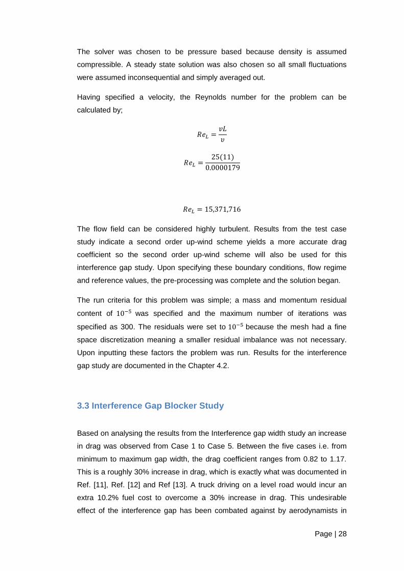
Having specified a velocity, the Reynolds number for the problem can be

calculated by;

The flow field can be considered highly turbulent. Results from the test case

study indicate a second order up-wind scheme yields a more accurate drag

coefficient so the second order up-wind scheme will also be used for this

interference gap study. Upon specifying these boundary conditions, flow regime

and reference values, the pre-processing was complete and the solution began.

The run criteria for this problem was simple; a mass and momentum residual

content of was specified and the maximum number of iterations was

specified as 300. The residuals were set to because the mesh had a fine

space discretization meaning a smaller residual imbalance was not necessary.

Upon inputting these factors the problem was run. Results for the interference

gap study are documented in the Chapter 4.2.

3.3 Interference Gap Blocker Study

Based on analysing the results from the Interference gap width study an increase

in drag was observed from Case 1 to Case 5. Between the five cases i.e. from

minimum to maximum gap width, the drag coefficient ranges from 0.82 to 1.17.

This is a roughly 30% increase in drag, which is exactly what was documented in

Ref. [11], Ref. [12] and Ref [13]. A truck driving on a level road would incur an

extra 10.2% fuel cost to overcome a 30% increase in drag. This undesirable

effect of the interference gap has been combated against by aerodynamists in

Page | 29

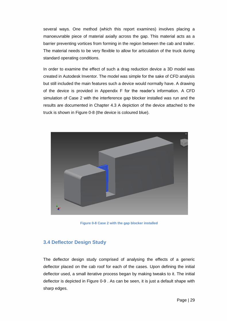
several ways. One method (which this report examines) involves placing a

manoeuvrable piece of material axially across the gap. This material acts as a

barrier preventing vortices from forming in the region between the cab and trailer.

The material needs to be very flexible to allow for articulation of the truck during

standard operating conditions.

In order to examine the effect of such a drag reduction device a 3D model was

created in Autodesk Inventor. The model was simple for the sake of CFD analysis

but still included the main features such a device would normally have. A drawing

of the device is provided in Appendix F for the reader’s information. A CFD

simulation of Case 2 with the interference gap blocker installed was run and the

results are documented in Chapter 4.3 A depiction of the device attached to the

truck is shown in Figure 0-8 (the device is coloured blue).

Figure 0-8 Case 2 with the gap blocker installed

3.4 Deflector Design Study

The deflector design study comprised of analysing the effects of a generic

deflector placed on the cab roof for each of the cases. Upon defining the initial

deflector used, a small iterative process began by making tweaks to it. The initial

deflector is depicted in Figure 0-9 . As can be seen, it is just a default shape with

sharp edges.

Page | 30

Figure 0-9 Initial deflector design

Design Method

The shape of the deflector outlined in Figure 0-9. is that of an extruded ellipse.

The exact dimensions used are shown in the drawing in Appendix G. When

creating the geometry one constraint was the deflector height was set to the

same height as the trailer. This was done because a smoother flow-field could be

created if the flow didn’t reach a stagnation point at the trailer front face. The

deflector width was chosen so it fitted neatly on the cab roof.

The deflector design study mainly involved the datum case but one test involved

replicating the gap width investigation with the deflector used in each case. This

was done to see what the resulting curve would look like i.e. would it follow the

previous curve with no deflector but with lower drag coefficient at each data point.

Obtaining this information was the first part of this particular study.

Deflector Optimization

The second part to the study was the design iteration process based on the initial

deflector. An overall drag coefficient was calculated for the initial deflector in the

first part. The objective of the second part was to improve on this. With this in

mind the default design was brought back into Inventor for remodelling. The first

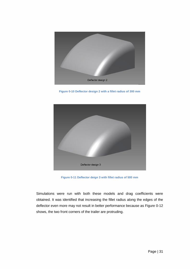
change made was an edit to the two side edges. A fillet of radius 300 mm was

used on the model and then a fillet of radius 500mm. The appearance of the

deflector with these two modifications can be seen in Figure 0-10 and Figure 0-11

Page | 31

Figure 0-10 Deflector design 2 with a fillet radius of 300 mm

Figure 0-11 Deflector deign 3 with fillet radius of 500 mm

Simulations were run with both these models and drag coefficients were

obtained. It was identified that increasing the fillet radius along the edges of the

deflector even more may not result in better performance because as Figure 0-12

shows, the two front corners of the trailer are protruding.

Page | 32

Figure 0-12 Datum truck with deflector 3 attached

Rounder fillet edges on the deflector would make more of the trailer vulnerable to

air-flow; this is unwanted because it would result in static pressure built up,

slowing down the truck and ultimately increasing in drag. So to counteract this

front corner problem, the fourth deflector design was modified to include two lugs

on the top left and right sides; Figure 0-13 shows this fourth design.

Figure 0-13 Deflector design 4

The two protruding ears along the top of the deflector prevent air-flow from

directly impinging on the trailer. They both have smooth features which should

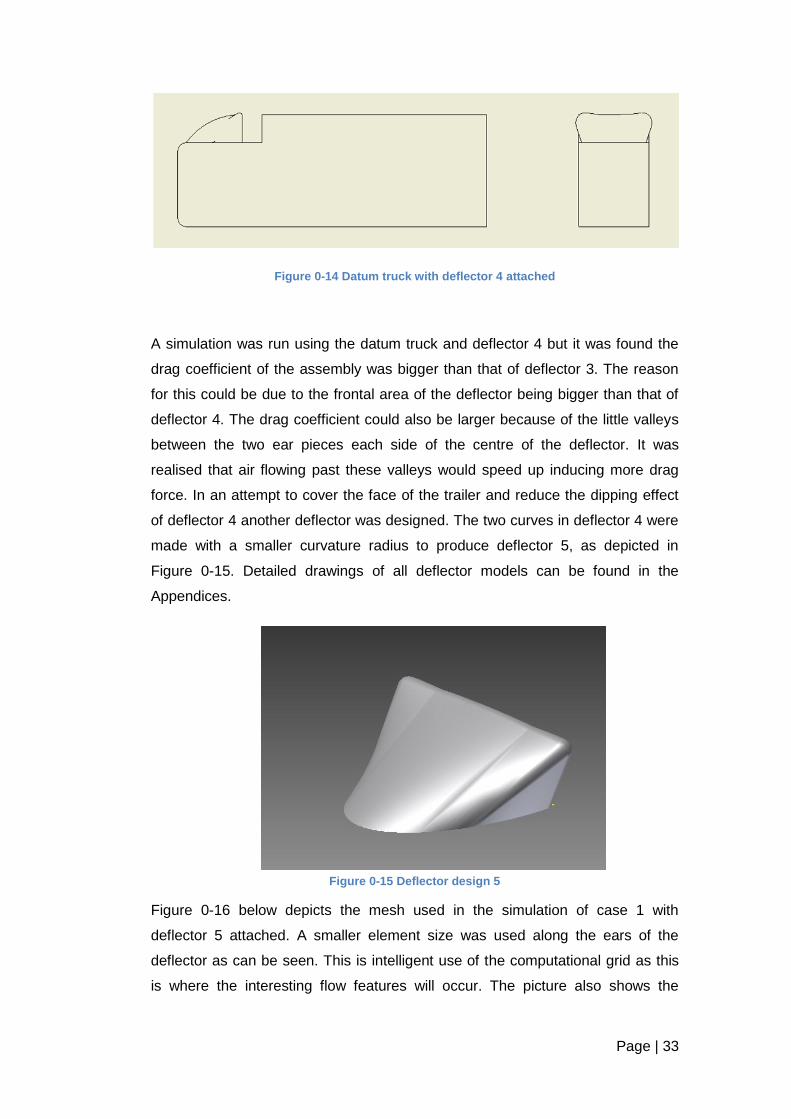
keep flow attached and reduce turbulence. Figure 0-14 shows how this deflector

covers the front face of the trailer entirely, as opposed to the third deflector

design.

Page | 33

Figure 0-14 Datum truck with deflector 4 attached

A simulation was run using the datum truck and deflector 4 but it was found the

drag coefficient of the assembly was bigger than that of deflector 3. The reason

for this could be due to the frontal area of the deflector being bigger than that of

deflector 4. The drag coefficient could also be larger because of the little valleys

between the two ear pieces each side of the centre of the deflector. It was

realised that air flowing past these valleys would speed up inducing more drag

force. In an attempt to cover the face of the trailer and reduce the dipping effect

of deflector 4 another deflector was designed. The two curves in deflector 4 were

made with a smaller curvature radius to produce deflector 5, as depicted in

Figure 0-15. Detailed drawings of all deflector models can be found in the

Appendices.

Figure 0-15 Deflector design 5

Figure 0-16 below depicts the mesh used in the simulation of case 1 with

deflector 5 attached. A smaller element size was used along the ears of the

deflector as can be seen. This is intelligent use of the computational grid as this

is where the interesting flow features will occur. The picture also shows the

Page | 34

layered cells along the surfaces of the truck. It is important to have a structured

grid here for the near wall treatment of the truck.

Figure 0-16 Mesh refinement of case 1 with deflector 5

3.5 Cross-wind study

The methodology defined for each of the simulations thus far have been for a

truck operating in still air conditions, i.e. they didn’t take into account wind

attacking the truck from an angle. This zero angle between the truck and wind

direction is known as the zero yaw angle, which gives insufficient indication of

aerodynamic characteristics in real world operation [3]. Incorporating a cross-

wind element to the aerodynamic analysis means introducing tangential force

components. This additional tangential force adds to the aerodynamic drag on

the truck. Figure 0-17 shows two pictures of a truck, one with wind at a zero yaw

angle (still air) and one with an incoming crosswind at angle θ°.

Page | 35

Figure 0-17 Comparison of a truck in still air (a) and one with a cross-wind at angle θ°

Geometry Setup

For this investigation of cross-wind influence the datum case will be used in the

simulations. The geometry used here is identical to that used in the datum case

of zero yaw angle. There is one issue though; the use of symmetry that was

applied to the datum case in the interference gap investigation couldn’t be used

here. This is because the incoming wind isn’t symmetric about the axial centreline

of the truck. Without the beneficial plane of symmetry the control volume

enclosing the truck is literally doubled in size. Elements within the mesh now

have to be a much bigger size so the mesh stays within the 512,000 cell limit. It

must be clearly noted that allowing the elements a bigger size could have a

significant effect on results obtained. This was proved in a brief mesh size

investigation of which the results are recorded in Chapter 4.1

Mesh setup

The mesh in this investigation, just like the geometry, is very similar to that of the

previous studies. There is one difference in the mesh setup however; the named

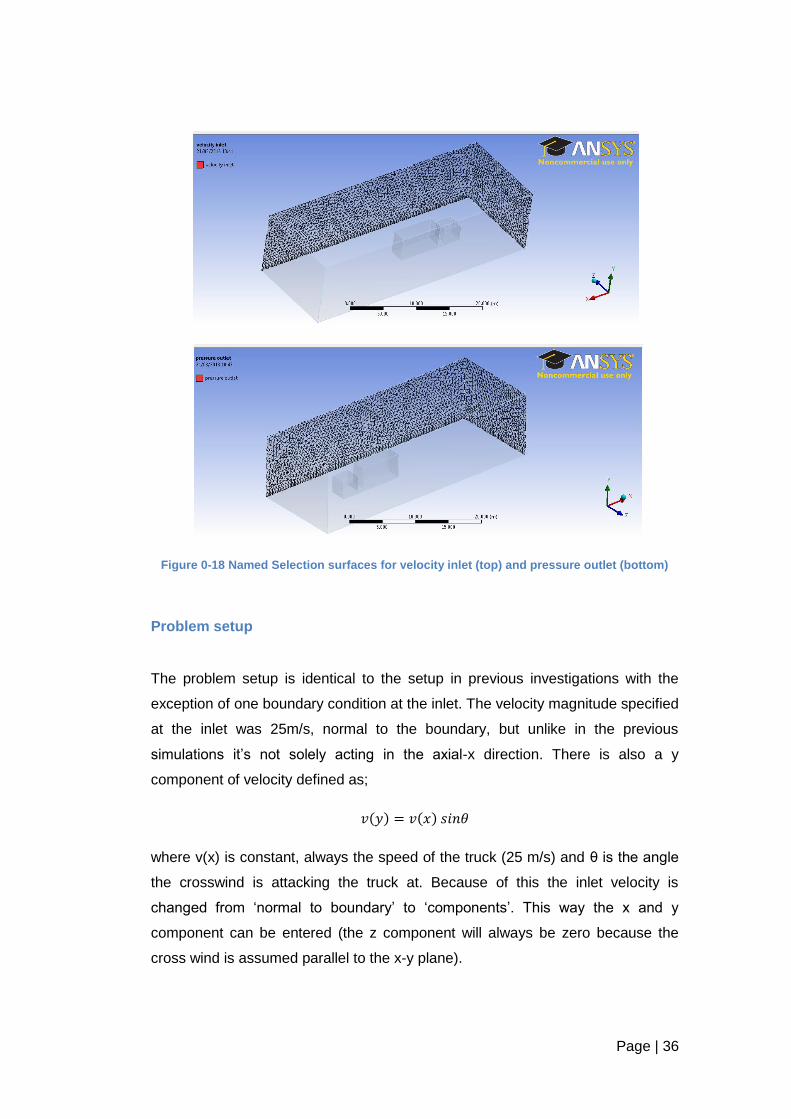
selections of the velocity inlet and pressure outlet. Because the flow is coming in

at angle relative to the axial direction the perpendicular inlet and outlet for the

previous investigations won’t suffice here. So instead the front and left plane

were made the velocity inlet and the rear and right planes were made the

pressure outlet. A visual representation of this is shown in Figure 0-18

Page | 36

Figure 0-18 Named Selection surfaces for velocity inlet (top) and pressure outlet (bottom)

Problem setup

The problem setup is identical to the setup in previous investigations with the

exception of one boundary condition at the inlet. The velocity magnitude specified

at the inlet was 25m/s, normal to the boundary, but unlike in the previous

simulations it’s not solely acting in the axial-x direction. There is also a y

component of velocity defined as;

where v(x) is constant, always the speed of the truck (25 m/s) and θ is the angle

the crosswind is attacking the truck at. Because of this the inlet velocity is

changed from ‘normal to boundary’ to ‘components’. This way the x and y

component can be entered (the z component will always be zero because the

cross wind is assumed parallel to the x-y plane).

Page | 37

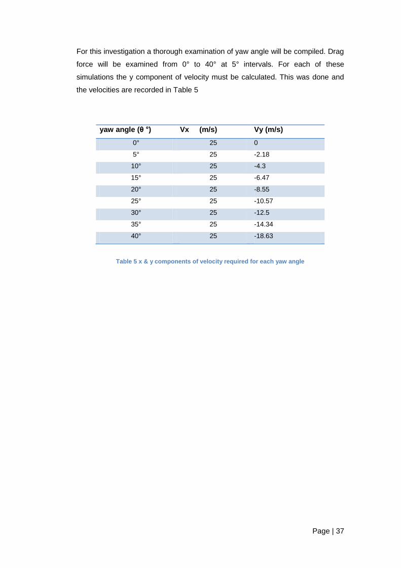
For this investigation a thorough examination of yaw angle will be compiled. Drag

force will be examined from 0° to 40° at 5° intervals. For each of these

simulations the y component of velocity must be calculated. This was done and

the velocities are recorded in Table 5

yaw angle (θ °) Vx (m/s) Vy (m/s)

0° 25 0

5° 25 -2.18

10° 25 -4.3

15° 25 -6.47

20° 25 -8.55

25° 25 -10.57

30° 25 -12.5

35° 25 -14.34

40° 25 -18.63

Table 5 x & y components of velocity required for each yaw angle

Page | 38

4. RESULTS AND DISCUSSION

4.1 The Cube

For the three meshes laminar and turbulent models along with first and second

order upwind solution methods were tested. The results are documented below in

Figure 4-0-1,Table 6, Table 7 and Table 8.

Figure 4-0-1 Mesh, flow regime and upwind scheme comparison

Figure 4-0-1 shows a convergence point at mesh 3. Mesh 1 and 2 show high

fluctuations between the parameters whereas mesh 3 appears to have more

concise results. This would indicate the results at that point are more accurate

than the two previous meshes. Based on the calculated drag coefficients in Table

x for mesh 3 the realizable k-epsilon model with non-equilibrium wall functions

will be used for the flow regime in subsequent truck model simulations. This is

because the resulting drag coefficient of 1.02 is the closest to Whites drag

coefficient of 1.07 for the flow past a cube under similar conditions.

0

0.2

0.4

0.6

0.8

1

1.2

1.4

1.6

0 200,000 400,000

Dra

g c

oeff

ecie

nt

Grid size (number of elements)

Computed drag coeffecient Vs. Mesh Size

1st order upwind:Laminar model

1st order upwind:Realiizable k-e modelwith non-equilibriumwall functions

2nd order upwind:Laminar model

2nd order upwind:Realiizable k-e modelwith non-equlibriumwall functions

Page | 39

Mesh 1 Drag coefficient

Turbulence model 1st order 2nd order

invisid 1.35 1.02

laminar 1.35 0.99

k-e (std & std) 1.35 1.05

k-e (std & non-equib) 1.35 1.03

k-e (realz & std) 1.36 1.05

k-e (realZ & non-equib) 1.36 1.03

Table 6 Mesh 1 drag coefficients for various turbulence models and upwind schemes

Mesh 2 Drag coefficient

Turbulence model 1st order 2nd order

invisid 1.13 0.99

laminar 1.13 0.98

k-e (std & std) 1.09 0.99

k-e (std & non-equib) 1.08 0.94

k-e (realz & std) 1.09 0.99

k-e (realz & non-equib) 1.08 1.01

Table 7 Mesh 2 drag coefficients for various turbulence models and upwind schemes

Mesh 3 Drag coefficient

Turbulence model 1st order 2nd order

invisid 1.02 1.03

laminar 1.02 1.03

k-e (std & std) 1.01 0.94

k-e (std & non-equib) 1.01 0.98

k-e (realz & std) 1 0.96

k-e (realz & non-equib) 1.02 1.02

Table 8 Mesh 3 drag coefficients for various turbulence models and upwind schemes

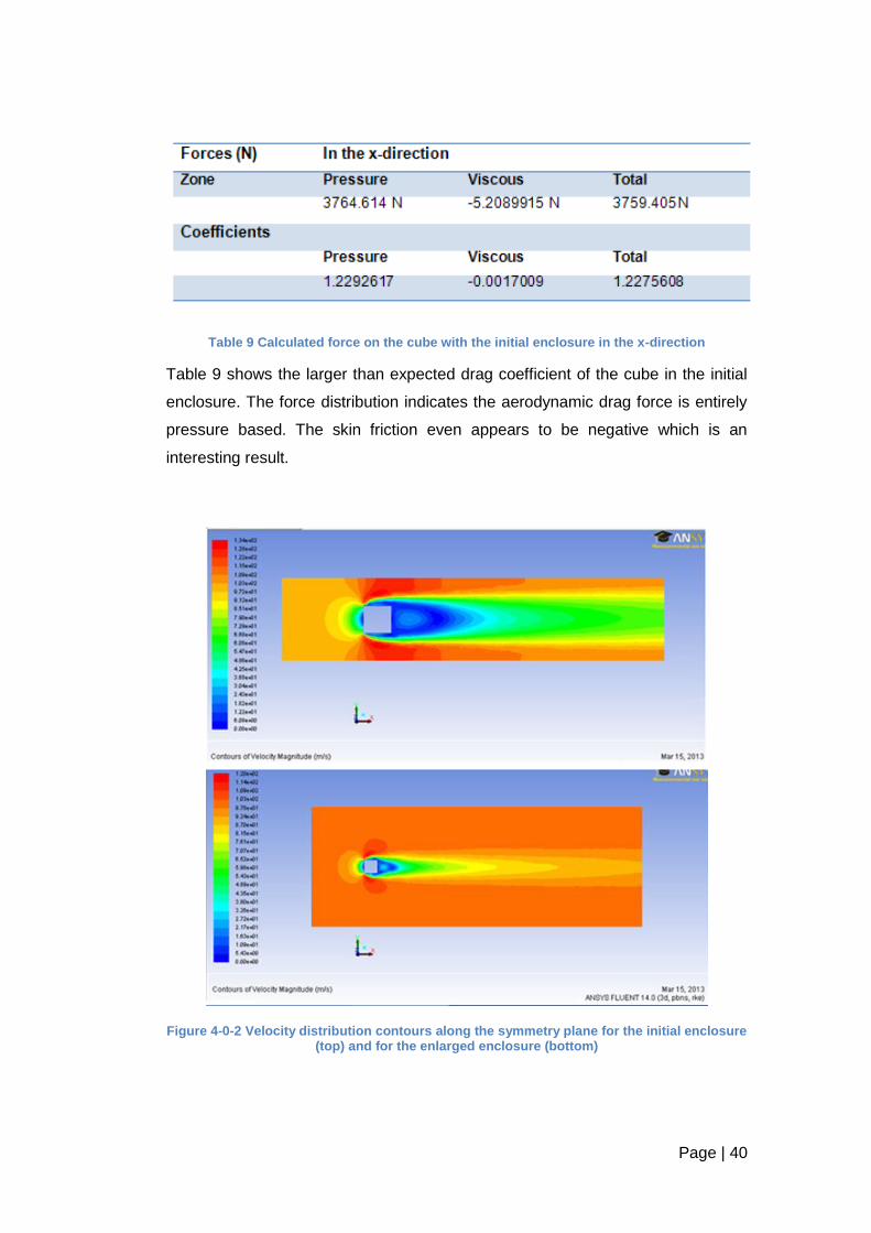
Page | 40

Table 9 Calculated force on the cube with the initial enclosure in the x-direction

Table 9 shows the larger than expected drag coefficient of the cube in the initial

enclosure. The force distribution indicates the aerodynamic drag force is entirely

pressure based. The skin friction even appears to be negative which is an

interesting result.

Figure 4-0-2 Velocity distribution contours along the symmetry plane for the initial enclosure (top) and for the enlarged enclosure (bottom)

Page | 41

Figure 4-0-3 Pressure distribution contours along the symmetry plane from the initial enclosure (top) enlarged enclosure (bottom)

The velocity contours for the initial enclosure show a much faster speed of air

past the cube. It was established that this was caused by the pushing of the air

past the cube so the laws of mass conservation would be obeyed. The cube

demonstrated a blocking effect within the enclosure; this was mentioned as one

of the problems real wind tunnels experience. The air in the larger enclosure is

allowed to flow freely; this means it will exert a smaller drag force on the cube.

This effect can also be seen in the pressure contours of Figure 4-0-3

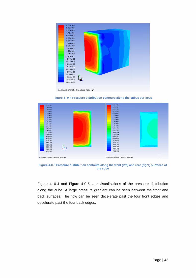
Page | 42

Figure 4--0-4 Pressure distribution contours along the cubes surfaces

Figure 4-0-5 Pressure distribution contours along the front (left) and rear (right) surfaces of the cube

Figure 4--0-4 and Figure 4-0-5. are visualizations of the pressure distribution

along the cube. A large pressure gradient can be seen between the front and

back surfaces. The flow can be seen decelerate past the four front edges and

decelerate past the four back edges.

Page | 43

4.2 Interference Gap Investigation

As Figure 0-5 showed, the gap between the tractor and trailer can account for

around 20% of the trucks total drag. A CFD simulation attempted to simulate this

influence using 5 data points, (Cases 1-5) each case having a bigger gap

between the cab and trailer. The manner in which the gap width is documented is

in terms of the ratio between the overall truck height (h) and the actual gap width

(b) as previously defined.

The first simulation of the datum case was computed using the methodology

outlined in Chapter 3. The recorded drag force, its skin friction and pressure

components and its non-dimensional coefficient are shown in Table 10. Once the

drag force was calculated the drag coefficient can be confirmed analytically via

the equation;

Where D is the drag coefficient, FD is the drag force, A is the projected area of

the truck in the direction of vehicle motion, ρ is the fluid density and v is the

trucks velocity.

According to Table 10 the computer recorded a drag force of 1569.03 N.

Substituting the values already defined in Table 10 into this equation results in a

coefficient of 0.82. This result confirms how the computer derives the drag

coefficient based on its calculation for the drag force as both coefficients

calculated are identical.

Figure 4-0-6 Influence of the growing interference gap on drag and Table 11

shows an increasing drag coefficient with increasing gap width. This was

expected to occur due to the increasing exposure of the trailer face to the

incoming wind. When more of the trailer face is exposed to the flow it results in

more stagnant pressure built up on the vehicle, ultimately slowing it down. Table

11 also indicates virtually no contribution of friction drag. The resulting forces are

all pressure based.

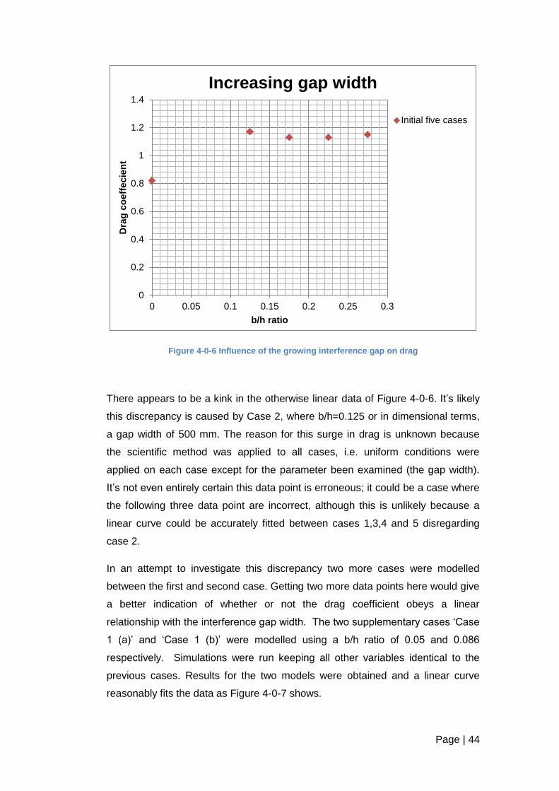
Page | 44

Figure 4-0-6 Influence of the growing interference gap on drag

There appears to be a kink in the otherwise linear data of Figure 4-0-6. It’s likely

this discrepancy is caused by Case 2, where b/h=0.125 or in dimensional terms,

a gap width of 500 mm. The reason for this surge in drag is unknown because

the scientific method was applied to all cases, i.e. uniform conditions were

applied on each case except for the parameter been examined (the gap width).

It’s not even entirely certain this data point is erroneous; it could be a case where

the following three data point are incorrect, although this is unlikely because a

linear curve could be accurately fitted between cases 1,3,4 and 5 disregarding

case 2.

In an attempt to investigate this discrepancy two more cases were modelled

between the first and second case. Getting two more data points here would give

a better indication of whether or not the drag coefficient obeys a linear

relationship with the interference gap width. The two supplementary cases ‘Case

1 (a)’ and ‘Case 1 (b)’ were modelled using a b/h ratio of 0.05 and 0.086

respectively. Simulations were run keeping all other variables identical to the

previous cases. Results for the two models were obtained and a linear curve

reasonably fits the data as Figure 4-0-7 shows.

0

0.2

0.4

0.6

0.8

1

1.2

1.4

0 0.05 0.1 0.15 0.2 0.25 0.3

Dra

g c

oeff

ecie

nt

b/h ratio

Increasing gap width

Initial five cases

Page | 45

Figure 4-0-7Gap width vs b/h ratio using two more cases

As Figure 4-0-7 shows, a reasonable linear relationship is exhibited by the drag

coefficient and the gap width. The data doesn’t fit perfectly on the curve as can

be seen from the trend-line; this could be due to inaccuracies within the CFD

code since all parameters were kept uniform for each test.

Recorded in Table 10 and Table 11 are the drag force and drag coefficients for

the five initial cases. These forces encapsulate the entire force the truck is

subject to, but it is unclear of the influence each surface has on it. For the datum

case a more detailed analysis was carried out on the distribution of force along

each of the individual surfaces of the truck. This breakdown is recorded in Table

12 and upon analysis of the figures an important observation can be made; the

majority of the surfaces have either zero pressure drag or zero skin friction. This

phenomenon was discussed in Chapter 1.

0

0.2

0.4

0.6

0.8

1

1.2

1.4

0 0.1 0.2 0.3

Dra

g c

oeff

ecie

nt

b/h ratio

Increasing gap width

Initial five cases

Case 1(a) & Case 1 (b)

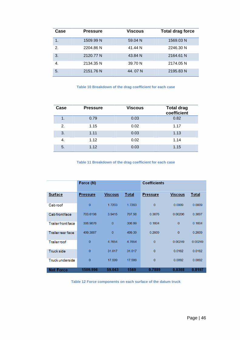
Page | 46

Case Pressure Viscous Total drag force

1. 1509.99 N 59.04 N 1569.03 N

2. 2204.86 N 41.44 N 2246.30 N

3. 2120.77 N 43.84 N 2164.61 N

4. 2134.35 N 39.70 N 2174.05 N

5. 2151.76 N 44. 07 N 2195.83 N

Table 10 Breakdown of the drag coefficient for each case

Case Pressure Viscous Total drag coefficient

1. 0.79 0.03 0.82

2. 1.15 0.02 1.17

3. 1.11 0.03 1.13

4. 1.12 0.02 1.14

5. 1.12 0.03 1.15

Table 11 Breakdown of the drag coefficient for each case

Table 12 Force components on each surface of the datum truck

Page | 47

Figure 4-0-8 Pressure distribution contours on the front (a) and rear (b) surfaces of the datum truck

Figure 4-0-8 shows the pressure distribution along the front and rear surfaces of

the datum truck. The pressure gradient between the front and back of the truck

can clearly be seen via the colours. The blue colours along the top and bottom of

the cabs front face indicate the lowest pressure. This is caused by the flows

change in direction over the truck resulting in an increased acceleration of the

flow. Bernoulli’s energy equation for a flow-field implies where velocity is high

pressure is low. This is the reason there is such low pressure on the front edges

of the truck.

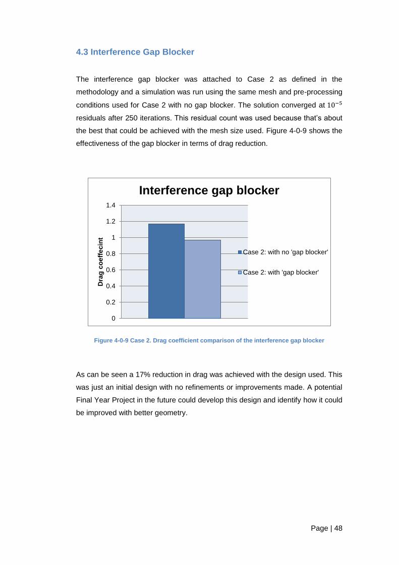
Page | 48

4.3 Interference Gap Blocker

The interference gap blocker was attached to Case 2 as defined in the

methodology and a simulation was run using the same mesh and pre-processing

conditions used for Case 2 with no gap blocker. The solution converged at

residuals after 250 iterations. This residual count was used because that’s about

the best that could be achieved with the mesh size used. Figure 4-0-9 shows the

effectiveness of the gap blocker in terms of drag reduction.

Figure 4-0-9 Case 2. Drag coefficient comparison of the interference gap blocker

As can be seen a 17% reduction in drag was achieved with the design used. This

was just an initial design with no refinements or improvements made. A potential

Final Year Project in the future could develop this design and identify how it could

be improved with better geometry.

0

0.2

0.4

0.6

0.8

1

1.2

1.4

Dra

g c

oeff

ecin

t

Interference gap blocker

Case 2: with no 'gap blocker'

Case 2: with 'gap blocker'

Page | 49

4.4 Deflector Investigation

As outlined in the methodology the first deflector was attached to each of the

varying gap width cases and simulations were run using the same mesh and

initialization. The results of this study are documented in Figure 4-0-10.

Figure 4-0-10 Drag coefficient vs varying gap width of the models with and without the deflector

Table 13 below is a record of each drag coefficient for each case with and without

the deflector. The percentage drag reduction is also given for the difference in

drag between each case. As can be seen an overall drag reduction of

approximately 20% can be achieved with this basic deflector.

Case 1. Case 2. Case 3. Case 4. Case 5.

No deflector CD 0.82 1.17 1.13 1.13 1.15

deflector 1 CD 0.66 0.88 0.85 0.96 0.97

% drag reduction 19.51% 24.79% 24.79% 15.04% 15.65%

net reduction 19.95%

Table 13 Drag reduction of deflector 1

0

0.2

0.4

0.6

0.8

1

1.2

1.4

0 0.1 0.2 0.3

Dra

g c

oe

ffecie

nt

h/b ratio

Increasing gap width

Initial fivecases

Initial fivecases withDeflector 1.

Page | 50

The second part of the deflector design study was the iterative process of

improving the initial wind deflector design. The datum case was run with each

deflector and the results of the simulations are shown in Figure 4-0-11. The most

noticeable aspect of the graph is the remarkable decrease in drag with each

iteration. The graph shows just how influential the shape of an object is with

regards to aerodynamics. A few simple geometric changes to the initial deflector

reduces the drag from 0.82 to 0.58; this is a 30% reduction. The fourth deflector

wasn’t as good as the second, third or fifth as can be seen. As already mentioned

in Chapter 3.4 this could be due to the increase in its projected area coupled with

the two valleys grooved into its design.

Figure 4-0-11 Drag coefficients of each deflector on the datum case.

Case 1: Drag coefficient Deflector type

0.82 no deflector

0.66 deflector (1)

0.67 deflector (2)

0.63 deflector (3)

0.69 deflector (4)

0.58 deflector (5)

Table 14 Drag coefficients of each deflector

0

0.1

0.2

0.3

0.4

0.5

0.6

0.7

0.8

0.9

no deflector deflector (1) deflector (2) deflector (3) deflector (4) deflector (5)

Dra

g c

oeff

ecie

nt

Deflector design drag coeffecients

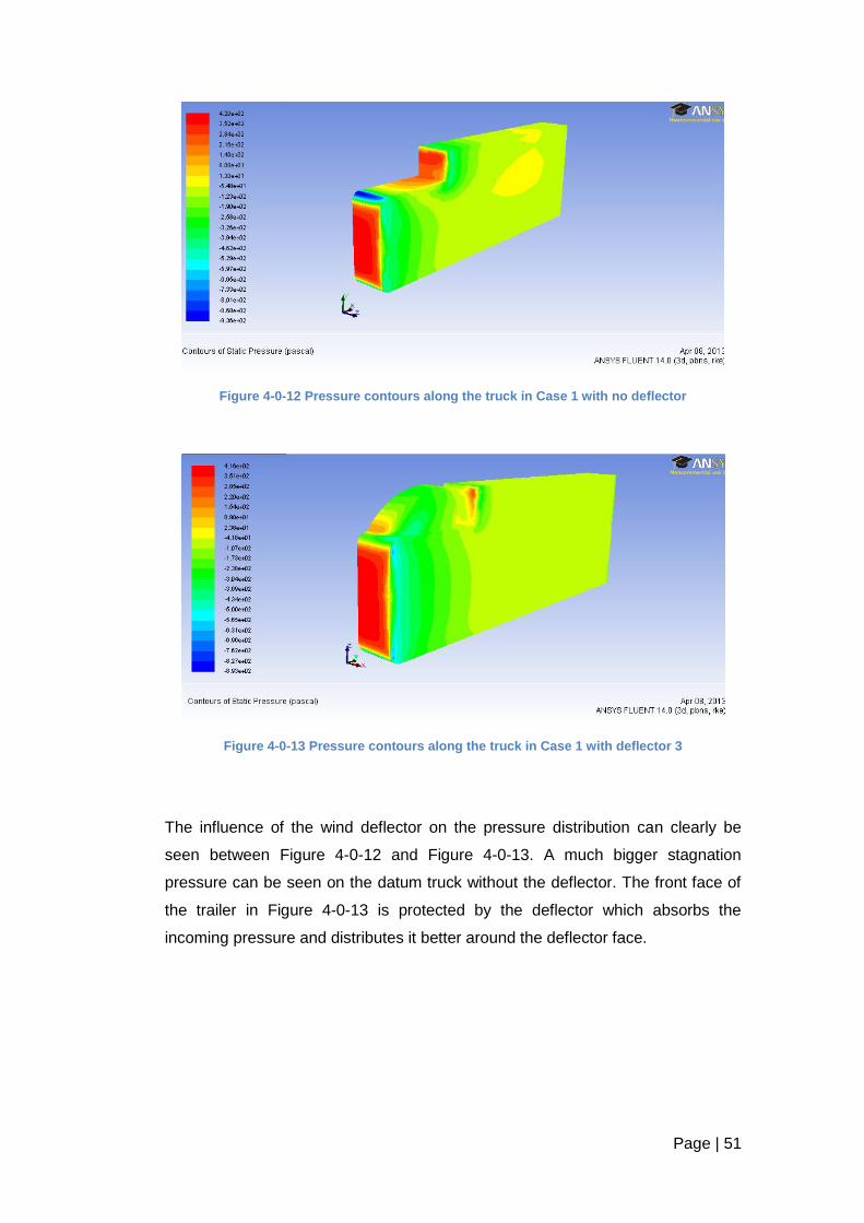
Page | 51

Figure 4-0-12 Pressure contours along the truck in Case 1 with no deflector

Figure 4-0-13 Pressure contours along the truck in Case 1 with deflector 3

The influence of the wind deflector on the pressure distribution can clearly be

seen between Figure 4-0-12 and Figure 4-0-13. A much bigger stagnation

pressure can be seen on the datum truck without the deflector. The front face of

the trailer in Figure 4-0-13 is protected by the deflector which absorbs the

incoming pressure and distributes it better around the deflector face.

Page | 52

4.5 Crosswind Investigation

The crosswind study was successful to a large extent. Numerical results obtained

compared well against experimental results documented in [3]. Figure 4-0-14

shows how drag varies with yaw angle for a range of commercial vehicles. Figure

4-0-15 below this shows the comparison of drag and yaw Fluent calculated in

each of the simulations.

Figure 4-0-14 Drag vs. yaw angle of different vehicle types

Figure 4-0-15 Calculated drag coefficient Vs. Yaw angle for the datum truck

0

0.5

1

1.5

2

2.5

0 10 20 30 40 50

Dra

g c

oeff

ecie

nt

Yaw angle (°)

Drag coeffecient Vs. Yaw angle

Page | 53

Case 1

Drag coefficient

Yaw angle

0.92 0°

1.63 5°

1.72 10°

1.84 25°

1.88 20°

1.89 25°

1.78 30°

1.65 35°

1.27 40°

Table 15 Documentation of the drag coefficient for each angle

In order to fully investigate the aerodynamic effects at play with the crosswind

simulations, a cutting plane was created in the Fluent post-processor. This plane

was cut one meter above the bottom of the truck as depicted in Figure 4-0-16.

Figure 4-0-16 Cutting plane used in the simulations

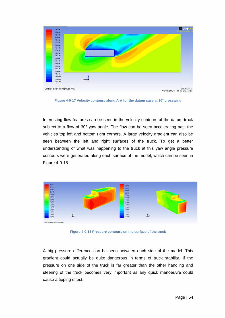
Page | 54

Figure 4-0-17 Velocity contours along A-A for the datum case at 30° crosswind

Interesting flow features can be seen in the velocity contours of the datum truck

subject to a flow of 30° yaw angle. The flow can be seen accelerating past the

vehicles top left and bottom right corners. A large velocity gradient can also be

seen between the left and right surfaces of the truck. To get a better

understanding of what was happening to the truck at this yaw angle pressure

contours were generated along each surface of the model, which can be seen in

Figure 4-0-18.

Figure 4-0-18 Pressure contours on the surface of the truck

A big pressure difference can be seen between each side of the model. This

gradient could actually be quite dangerous in terms of truck stability. If the

pressure on one side of the truck is far greater than the other handling and

steering of the truck becomes very important as any quick manoeuvre could

cause a tipping effect.

Page | 55

The second part of the crosswind study involved the same analysis for Case 5.

The same cutting plane was created for investigating the velocity and pressure

distributions. Figure 4-0-19 below shows the velocity vectors along the A-A plane

at 30° yaw angle.

Figure 4-0-19 Velocity vectors along A-A at 30° yaw angle for Case 5 (PLAN VIEW)

It is interesting to note the passage of flow through the interference gap. The flow

is relatively faster through the gap and around the right corner of the cab.

Vortices cab be seen forming to the right hand side of the cab and trailer.

Figure 4-0-20 Pressure coefficient contours along A-A at 30° yaw angle of Case 5 (PLAN VIEW)

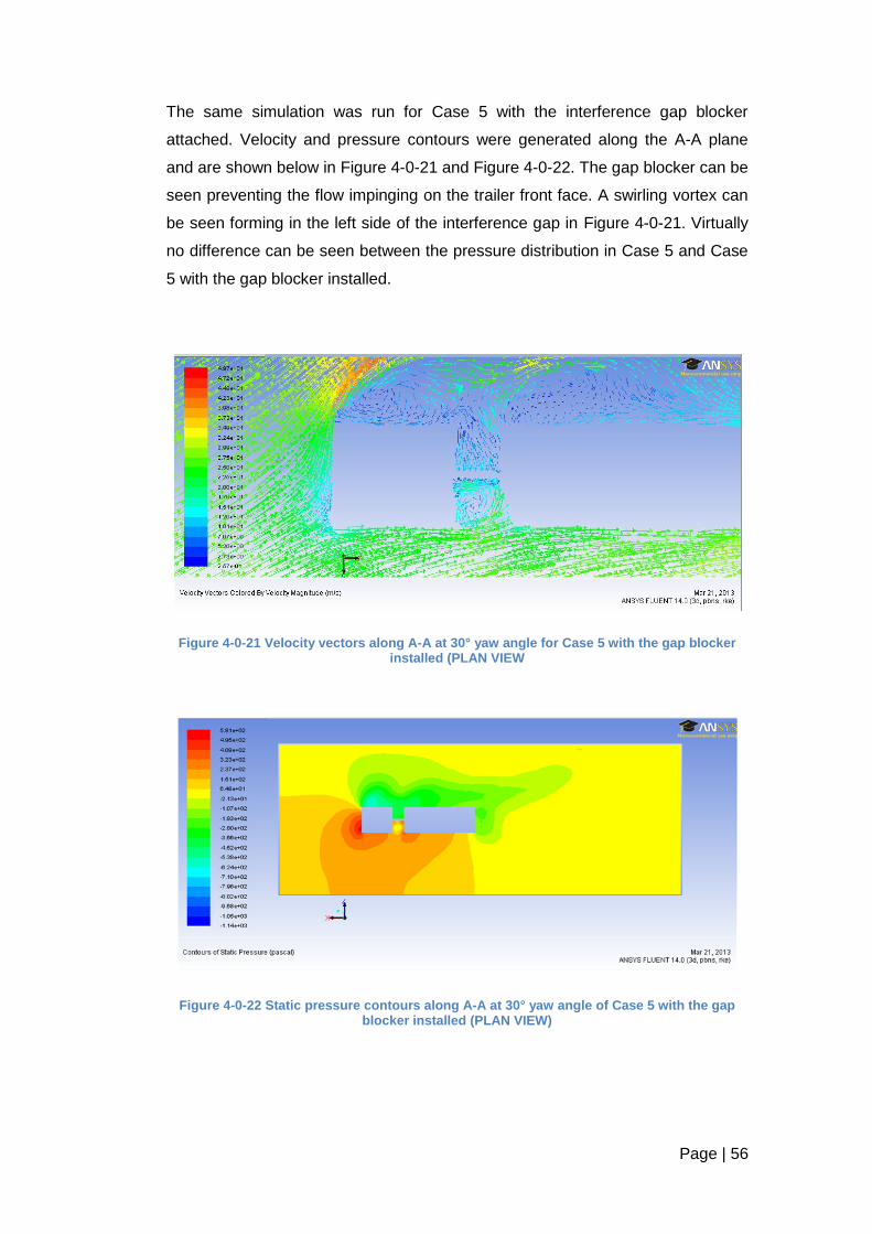
Page | 56

The same simulation was run for Case 5 with the interference gap blocker

attached. Velocity and pressure contours were generated along the A-A plane

and are shown below in Figure 4-0-21 and Figure 4-0-22. The gap blocker can be

seen preventing the flow impinging on the trailer front face. A swirling vortex can

be seen forming in the left side of the interference gap in Figure 4-0-21. Virtually

no difference can be seen between the pressure distribution in Case 5 and Case

5 with the gap blocker installed.

Figure 4-0-21 Velocity vectors along A-A at 30° yaw angle for Case 5 with the gap blocker installed (PLAN VIEW

Figure 4-0-22 Static pressure contours along A-A at 30° yaw angle of Case 5 with the gap blocker installed (PLAN VIEW)

Page | 57

The pressure distribution along the truck was obtained for Case 5 with the gap

blocker installed and is shown in Figure 4-0-23 for the left hand side and in Figure

4-0-24 for the right hand side. The pressure distribution is very similar to that of

Case 5 without the gap blocker.

Figure 4-0-23 Pressure distribution along the left surface of the Case 5 truck with the gap blocker installed

Figure 4-0-24 Pressure distribution along the right surface of the Case 5 truck with the gap blocker installed

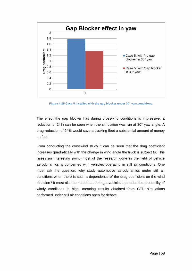
Page | 58

Figure 4-25 Case 5 installed with the gap blocker under 30° yaw conditions

The effect the gap blocker has during crosswind conditions is impressive; a

reduction of 24% can be seen when the simulation was run at 30° yaw angle. A

drag reduction of 24% would save a trucking fleet a substantial amount of money

on fuel.

From conducting the crosswind study it can be seen that the drag coefficient

increases quadratically with the change in wind angle the truck is subject to. This

raises an interesting point; most of the research done in the field of vehicle

aerodynamics is concerned with vehicles operating in still air conditions. One

must ask the question, why study automotive aerodynamics under still air

conditions when there is such a dependence of the drag coefficient on the wind

direction? It most also be noted that during a vehicles operation the probability of

windy conditions is high, meaning results obtained from CFD simulations

performed under still air conditions open for debate.

0

0.2

0.4

0.6

0.8

1

1.2

1.4

1.6

1.8

2

1

Dra

g c

oeff

ecie

nt

Gap Blocker effect in yaw

Case 5: with 'no gapblocker' in 30° yaw

Case 5: with 'gap blocker'in 30° yaw

Page | 59

4.6 Limitations

The biggest limitation encountered during the project was the maximum cell

count in Ansys Fluent. Only having 512,000 elements available to model full

scale trucks was very difficult. In the reports and journals reviewed for this project

the average number of elements used in typical CFD simulations for full scale

models was in the order of 5 million [12]. Due to the lack of cells, a true mesh

convergence studied was not possible and results for the mesh comparison in

this report established a 25% difference in the drag coefficient between Mesh 1

(21,000 elements) and Mesh 3 (490,000 elements). This implies the drag

coefficient is dependent on the mesh size and because of this, the accuracy of

the results obtained in this report are open to debate.

Another limitation encountered was the lack of a true validation case for the truck

models used. The meshes developed here are based on ones used in excellent

sources ([10] and [15]) but a rigorous validation and verification process is very

important with any CFD simulation.

During the first two months of the project Ansys Fluent wasn’t installed in the

computer suites meaning no CFD work could get done at all. This delayed the

project by two months which meant a lot of the simulations originally planned

couldn’t actually be done.

4.7 Recommendations for future work

All of the CFD models used in this project were all initial designs without much

refinement and optimization. This could be an area for further development; the

deflector design and the gap blocker geometry could be optimized

Page | 60

5. CONCLUSIONS

From the analysis conducted in this report some very important conclusions can

be drawn. The flow over an immersed bluff body is almost entirely pressure

based. The results show the contribution of skin friction to the overall drag

coefficient is negligible, less than 1% in most simulations. This implies that in

order to improve vehicle aerodynamics, the variables in the equation which

govern pressure drag are the only variables of importance when designing

aerodynamic blunt bodies. All types of trucks can be considered blunt bodies due

to their natural cuboid geometry.

When analysing the simulations of the cube it can be stated that for the given

mesh sizes used, little difference exists between any of the various flow regimes

used and any of the upwind solution schemes used. The drag coefficient

calculated, using an invisid model and first order upwind solution scheme for

Mesh 2, is only 10% off the drag coefficient calculated for Mesh 3 with a second

order upwind solution scheme, and realizable k-epsilon model. This small

difference poses an interesting question; how accurate does one want a solution

to be, given the extra computation cost and complexity of high quality meshes,

complicated turbulence models and higher order upwind schemes? For many

purposes a ballpark result within plus/minus 10% of the actual solution is

sufficient. This tolerance level however would not suffice in the design of drag

reduction devices because such devices would only improve drag by a maximum

of 30-50%, meaning every per cent is crucial.

With regard to enclosure design for cubes it was found that a small size results in

a blockage effect produced by the cube resulting in a higher drag coefficient due

to the pressurized force exerted by the air. Enlarging the enclosure eliminated

this effect and a similar solution to Whites was obtained. Analysis conducted on

the pressure contours of the cube showed a large pressure gradient between the

front face subject to the flow and the rear face in the wake of the flow; the reason

for this pressure gradient is explained in Chapter 1.

Results from the interference gap investigation indicate a linear relationship

between the drag coefficient and the gap width; this relationship needs further

confirmation however as none of the literature reviewed as part of this project

reported any relationship between drag and gap width. Upon analysing the

Page | 61

pressure distribution on each of the truck surfaces, it was observed that any

particular face of the truck was subject to either pressure drag or friction drag but

not both. The faces perpendicular to the flow were responsible for the pressure

drag and the faces tangential to the flow were responsible for the skin friction.

This is what was expected to happen as explained in Chapter 1.

The deflector design carried out as part of this project was successful in that drag

reduction of up to 30% was recorded with the models used. This study involved

an iterative design process but it never reached an optimization point for the

deflector geometry; this could be studied in more detail in a subsequent Final

Year Project.

The cross-wind study was also successful. Incoming wind impinging on the truck

at 5° angle intervals was studied. Monitors for the drag force in the axial direction

of the truck were created and solutions were examined and compared to ones

recorded by Hucho in [3]. Similar trends in the relationship between drag

coefficient and wind angle were observed between results recorded in this project

and those published by Hucho. In conclusion the increase in wind angle

corresponds to an increase in drag force up to an angle of approximately 20°

after which point it reduces by the same rate. The drag increase due to the wind

angle was combated via a drag reduction device placed in the interference gap.

At the 30° wind angle the gap blocker reduces the drag by 24% according to the

simulated results.

To conclude, there are enormous benefits to be gained from installing drag

reduction devices to Class 8 trucks. As stated in Chapter 1 fuel consumption is

dependent on aerodynamic drag, so by reducing the drag force by means of add-

on devices, trucking companies with fleets of fuel thirsty trucks can save

substantial money on fuel. There would also be knock-on beneficial

environmental effects.

Page | 62

REFERENCES

[5] R. Drollinger, Heavy duty truck aerodynamics, Society of Automotive

Engineers, 1987.

[6] Mu Wang1, Qiang Li, Dengfeng Wang, Changhai Yang, Jinlong Zhao, Guijin

Wen, “The Air-deflector and the drag: A Case Study of Low Drag Cab Styling

for a Heavy Truck,” Jinan, 2009.

[7] J. Eaton, “Session 26: Computational Fluid Dynamics,” Galway, 2013.

[8] F. White, Fluid Mechanics, WCB McGraw-Hill, 2005.

[9] Ansys, “Ansys Advantage Voulme 5 issue 1,” 2011.

[10] M. Lanfrit, “Best practice Guidlines for Handling Automotive External Vehicle

Aerodynamics with FLUENT,” Darmstadt, 2005.

[11] F. Browand, “Reducing Aerodynamic Drag and Fuel Consumption,” 2011.

[12] F.-H. Hsu, “Drag Reduction of Tractor-Trailers Using Optimized Add-On

Devices,” American Society of Mechanical Enginees, Los Angelas, 2010.

[13] Subrahmanya Veluri, Christopher Roy, “Joint Computational/Experimental

Aerodynamic Study of a Simplified Tractor/Trailer Geometry,” American

Society of Mechanical Engineers, Blacksburg, 2009.

[14] T. Favre, “Aerodynamic Simulations of ground vehicles in Unsteady

Crosswind,” 2011.

[15] F.-H. Hsu, “Design of Tractor-Trailer Add-On Drag Reduction Devices Using

CFD,” Los Angelas, 2009.

[1] Li Song, Zhang Jicheng, Liu Yongxue, Hu Tieyu, “Aerodynamic Drag Reduction Design of Van Body Truck by Numerical Simulation Method,” in Second International Conference on Digital Manufacturing & Automation, Changchun, 2011.

[2] U.S. Department of Energy, Transportation Energy Data Book, Oak Ridge, Tennesse, 2012.

[3] W.-H. Hucho, The Aerodynamcis of Road Vehicles, 1988.

[4] R. Wood, “A Discussion of a Heavy Truck Advanced Aerodynamic Trailer System,” 2010.

Page | 63

APPENDICES

Appendix A: Model Truck Case 1.

Appendix B: Model Truck Case 2.

Appendix C: Model Truck Case 3.

Appendix D: Model Truck Case 4.

Appendix E: Model Truck Case 5.

Appendix F: Interference Gap Blocker

Appendix G: Deflector Design 1.

Appendix H: Deflector Design 2.

Appendix I: Deflector Design 3.

Appendix J: Deflector Design 4.

Appendix K: Deflector Design 5.

Appendix L: Model Truck Assembly

Page | 64

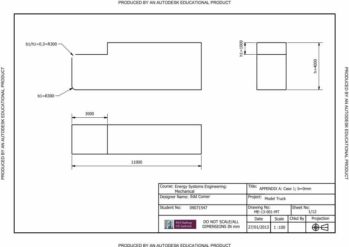
PRODUCED BY AN AUTODESK EDUCATIONAL PRODUCT

PRODUCED BY AN AUTODESK EDUCATIONAL PRODUCTP

RO

DU

CE

D B

Y A

N A

UT

OD

ES

K E

DU

CA

TIO

NA

L P

RO

DU

CT

PR

OD

UC

ED

B

Y A

N A

UT

OD

ES

K E

DU

CA

TIO

NA

L P

RO

DU

CT

Title:

Project:

Drawing No:

Date Scale

Projection

Designer Name:

Course:

Student No:

DO NOT SCALE/ALL

DIMENSIONS IN mm

Sheet No:

Chkd By

Energy Systems Engineering:

Mechanical

Edd Comer

09071547

APPENDIX A: Case 1; b=0mm

Model Truck

ME-13-001-MT

27/01/20131 :100

1/12

4000

h=

1000

h1=

11000

3000

R300b1/h1=0.3=

R300b1=

PRODUCED BY AN AUTODESK EDUCATIONAL PRODUCT

PRODUCED BY AN AUTODESK EDUCATIONAL PRODUCTP

RO

DU

CE

D B

Y A

N A

UT

OD

ES

K E

DU

CA

TIO

NA

L P

RO

DU

CT

PR

OD

UC

ED

B

Y A

N A

UT

OD

ES

K E

DU

CA

TIO

NA

L P

RO

DU

CT

Title:

Project:

Drawing No:

Date Scale

Projection

Designer Name:

Course:

Student No:

DO NOT SCALE/ALL

DIMENSIONS IN mm

Sheet No:

Chkd By

Energy Systems Engineering:

Mechanical

Edd Comer

09071547

APPENDIX B: Case 2, b=500mm

Model Truck

ME-13-002-MT

27/01/20131 :100

2/12

4000

h=

1000

h1=

400

500b=

2500

3000

11000

R300b1/h1=0.3=

R300b1=

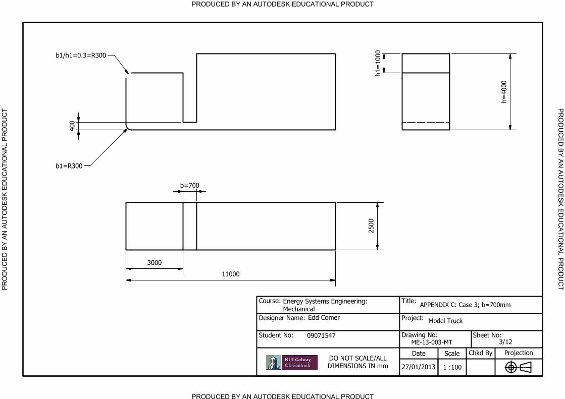
PRODUCED BY AN AUTODESK EDUCATIONAL PRODUCT

PRODUCED BY AN AUTODESK EDUCATIONAL PRODUCTP

RO

DU

CE

D B

Y A

N A

UT

OD

ES

K E

DU

CA

TIO

NA

L P

RO

DU

CT

PR

OD

UC

ED

B

Y A

N A

UT

OD

ES

K E

DU

CA

TIO

NA

L P

RO

DU

CT

Title:

Project:

Drawing No:

Date Scale

Projection

Designer Name:

Course:

Student No:

DO NOT SCALE/ALL

DIMENSIONS IN mm

Sheet No:

Chkd By

Energy Systems Engineering:

Mechanical

Edd Comer

09071547

APPENDIX C: Case 3; b=700mm

Model Truck

ME-13-003-MT

27/01/20131 :100

3/12

1000

h1=

4000

h=

2500

11000

400

R300b1/h1=0.3=

700b=

R300b1=

3000

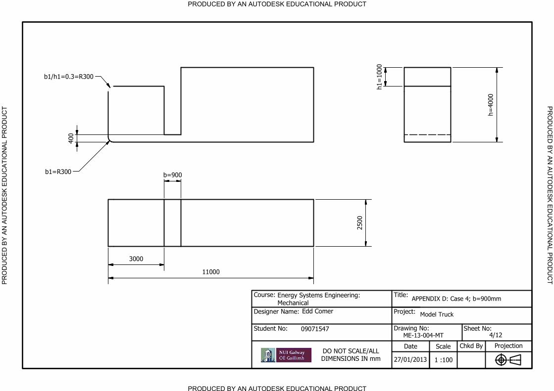
PRODUCED BY AN AUTODESK EDUCATIONAL PRODUCT

PRODUCED BY AN AUTODESK EDUCATIONAL PRODUCTP

RO

DU

CE

D B

Y A

N A

UT

OD

ES

K E

DU

CA

TIO

NA

L P

RO

DU

CT

PR

OD

UC

ED

B

Y A

N A

UT

OD

ES

K E

DU

CA

TIO

NA

L P

RO

DU

CT

Title:

Project:

Drawing No:

Date Scale

Projection

Designer Name:

Course:

Student No:

DO NOT SCALE/ALL

DIMENSIONS IN mm

Sheet No:

Chkd By

Energy Systems Engineering:

Mechanical

Edd Comer

09071547

APPENDIX D: Case 4; b=900mm

Model Truck

ME-13-004-MT

27/01/20131 :100

4/12

4000

h=

1000

h1=

400

2500

900b=

11000

3000

R300b1=

R300b1/h1=0.3=

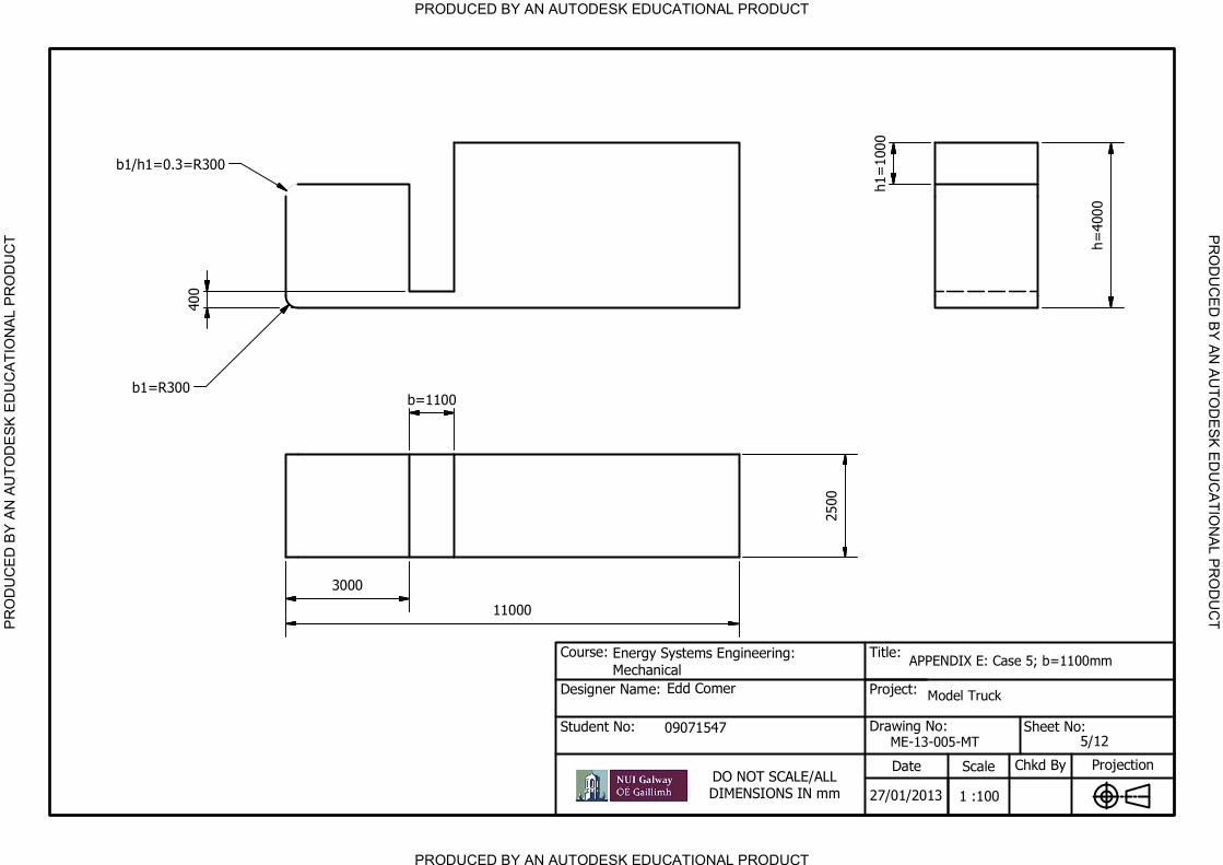
PRODUCED BY AN AUTODESK EDUCATIONAL PRODUCT

PRODUCED BY AN AUTODESK EDUCATIONAL PRODUCTP

RO

DU

CE

D B

Y A

N A

UT

OD

ES

K E

DU

CA

TIO

NA

L P

RO

DU

CT

PR

OD

UC

ED

B

Y A

N A

UT

OD

ES

K E

DU

CA

TIO

NA

L P

RO

DU

CT

Title:

Project:

Drawing No:

Date Scale

Projection

Designer Name:

Course:

Student No:

DO NOT SCALE/ALL

DIMENSIONS IN mm

Sheet No:

Chkd By

Energy Systems Engineering:

Mechanical

Edd Comer

09071547

APPENDIX E: Case 5; b=1100mm

Model Truck

ME-13-005-MT

27/01/20131 :100

5/12

4000

h=

1000

h1=

2500

1100b=

11000

3000

400

R300b1=

R300b1/h1=0.3=

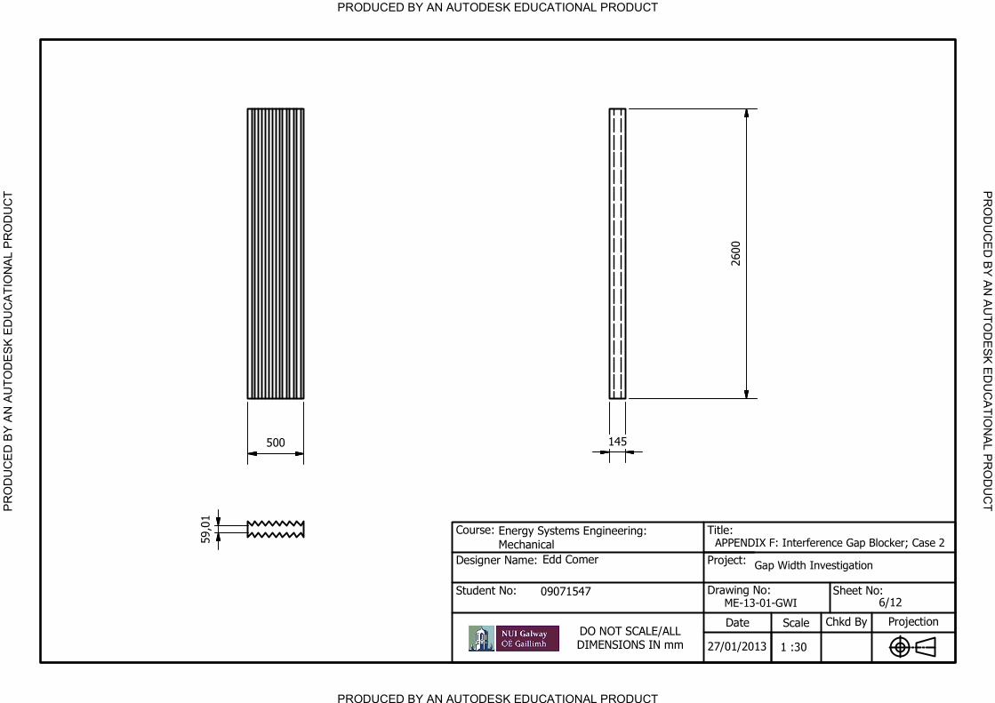
PRODUCED BY AN AUTODESK EDUCATIONAL PRODUCT

PRODUCED BY AN AUTODESK EDUCATIONAL PRODUCTP

RO

DU

CE

D B

Y A

N A

UT

OD

ES

K E

DU

CA

TIO

NA

L P

RO

DU

CT

PR

OD

UC

ED

B

Y A

N A

UT

OD

ES

K E

DU

CA

TIO

NA

L P

RO

DU

CT

Title:

Project:

Drawing No:

Date Scale

Projection

Designer Name:

Course:

Student No:

DO NOT SCALE/ALL

DIMENSIONS IN mm

Sheet No:

Chkd By

Energy Systems Engineering:

Mechanical

Edd Comer

09071547

APPENDIX F: Interference Gap Blocker; Case 2

Gap Width Investigation

ME-13-01-GWI

27/01/20131 :30

6/12

2600

145

500

59,01

PRODUCED BY AN AUTODESK EDUCATIONAL PRODUCT

PRODUCED BY AN AUTODESK EDUCATIONAL PRODUCTP

RO

DU

CE

D B

Y A

N A

UT

OD

ES

K E

DU

CA

TIO

NA

L P

RO

DU

CT

PR

OD

UC

ED

B

Y A

N A

UT

OD

ES

K E

DU

CA

TIO

NA

L P

RO

DU

CT

Title:

Project:

Drawing No:

Date Scale

Projection

Designer Name:

Course:

Student No:

DO NOT SCALE/ALL

DIMENSIONS IN mm

Sheet No:

Chkd By

Energy Systems Engineering:

Mechanical

Edd Comer

09071547

APPENDIX G: Deflector Design 1

Deflector Design Study

ME-13-01-DD

27/01/20131 :40

7/12

2000

1000

15

15

15

15

2300

15mm SHELLED INTERIOR

STANDARD ELLEPTICAL SHAPE

PRODUCED BY AN AUTODESK EDUCATIONAL PRODUCT

PRODUCED BY AN AUTODESK EDUCATIONAL PRODUCTP

RO

DU

CE

D B

Y A

N A

UT

OD

ES

K E

DU

CA

TIO

NA

L P

RO

DU

CT

PR

OD

UC

ED

B

Y A

N A

UT

OD

ES

K E

DU

CA

TIO

NA

L P

RO

DU

CT

Title:

Project:

Drawing No:

Date Scale

Projection

Designer Name:

Course:

Student No:

DO NOT SCALE/ALL

DIMENSIONS IN mm

Sheet No:

Chkd By

Energy Systems Engineering:

Mechanical

Edd Comer

09071547

APPENDIX H: Deflector Design 2

Deflector Design Study

ME-13-02-DD

27/01/20131 :40

8/12

2300

1000

2000

STANDARD ELLEPTICAL SHAPE

15 15

15

15

R300,052 FILLETS OF

15mm SHELLED INTERIOR

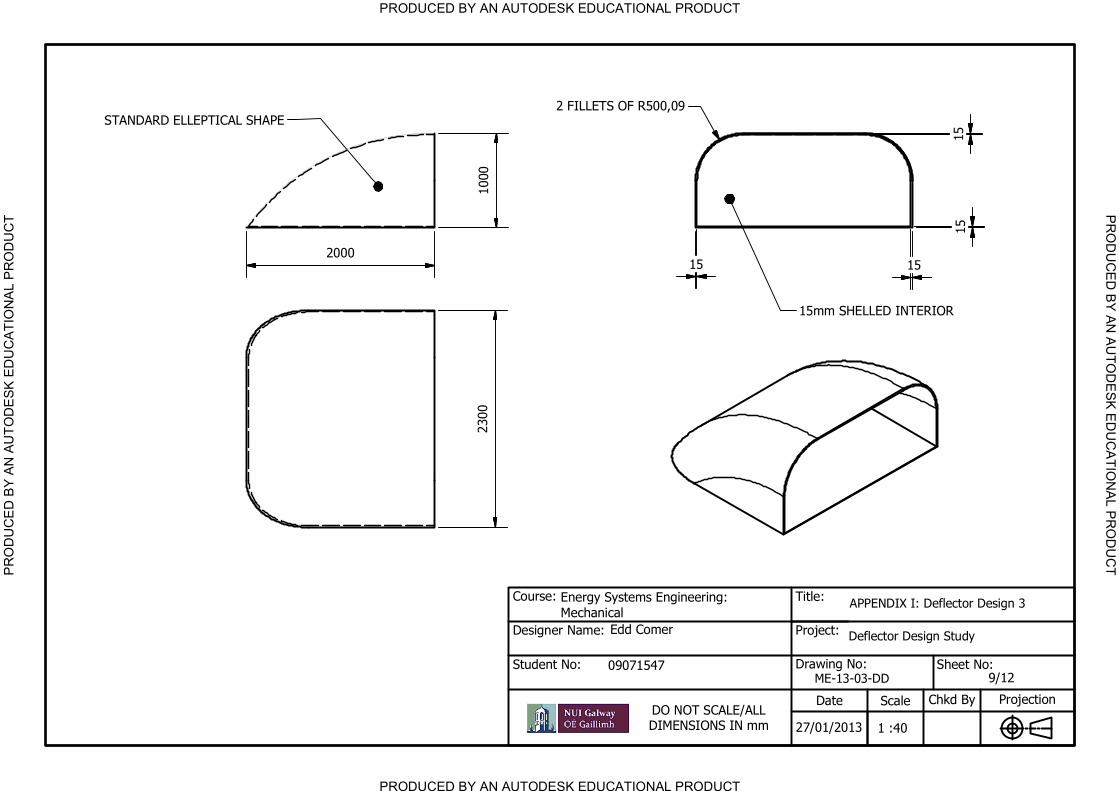
PRODUCED BY AN AUTODESK EDUCATIONAL PRODUCT

PRODUCED BY AN AUTODESK EDUCATIONAL PRODUCTP

RO

DU

CE

D B

Y A

N A

UT

OD

ES

K E

DU

CA

TIO

NA

L P

RO

DU

CT

PR

OD

UC

ED

B

Y A

N A

UT

OD

ES

K E

DU

CA

TIO

NA

L P

RO

DU

CT

Title:

Project:

Drawing No:

Date Scale

Projection

Designer Name:

Course:

Student No:

DO NOT SCALE/ALL

DIMENSIONS IN mm

Sheet No:

Chkd By

Energy Systems Engineering:

Mechanical

Edd Comer

09071547

APPENDIX I: Deflector Design 3

Deflector Design Study

ME-13-03-DD

27/01/20131 :40

9/12

2300

1000

2000

STANDARD ELLEPTICAL SHAPE

1515

15

15

R500,092 FILLETS OF

15mm SHELLED INTERIOR

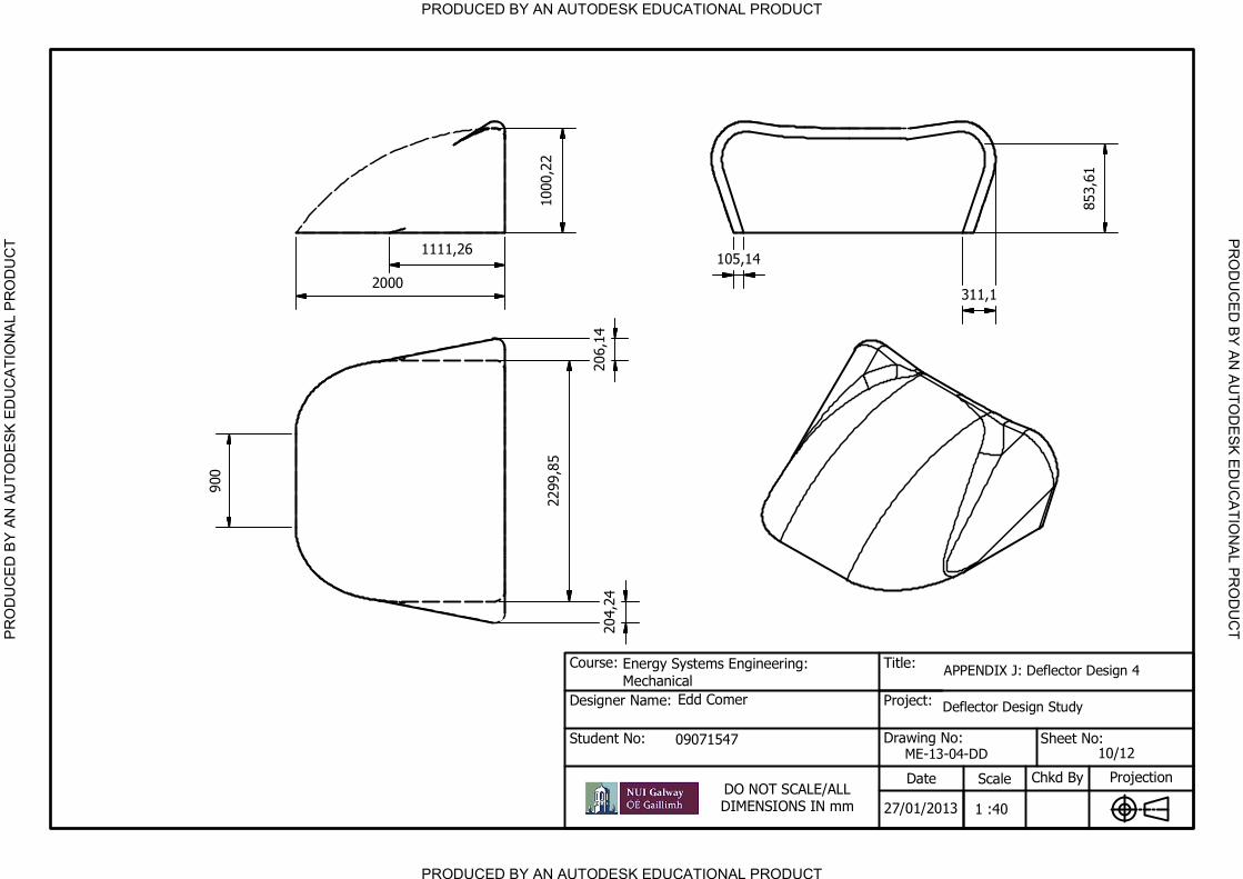
PRODUCED BY AN AUTODESK EDUCATIONAL PRODUCT

PRODUCED BY AN AUTODESK EDUCATIONAL PRODUCTP

RO

DU

CE

D B

Y A

N A

UT

OD

ES

K E

DU

CA

TIO

NA

L P

RO

DU

CT

PR

OD

UC

ED

B

Y A

N A

UT

OD

ES

K E

DU

CA

TIO

NA

L P

RO

DU

CT

Title:

Project:

Drawing No:

Date Scale

Projection

Designer Name:

Course:

Student No:

DO NOT SCALE/ALL

DIMENSIONS IN mm

Sheet No:

Chkd By

Energy Systems Engineering:

Mechanical

Edd Comer

09071547

APPENDIX J: Deflector Design 4

Deflector Design Study

ME-13-04-DD

27/01/20131 :40

10/12

2000

1000,22

2299,85

311,1

105,14

206,14

204,24

1111,26

900

853,61

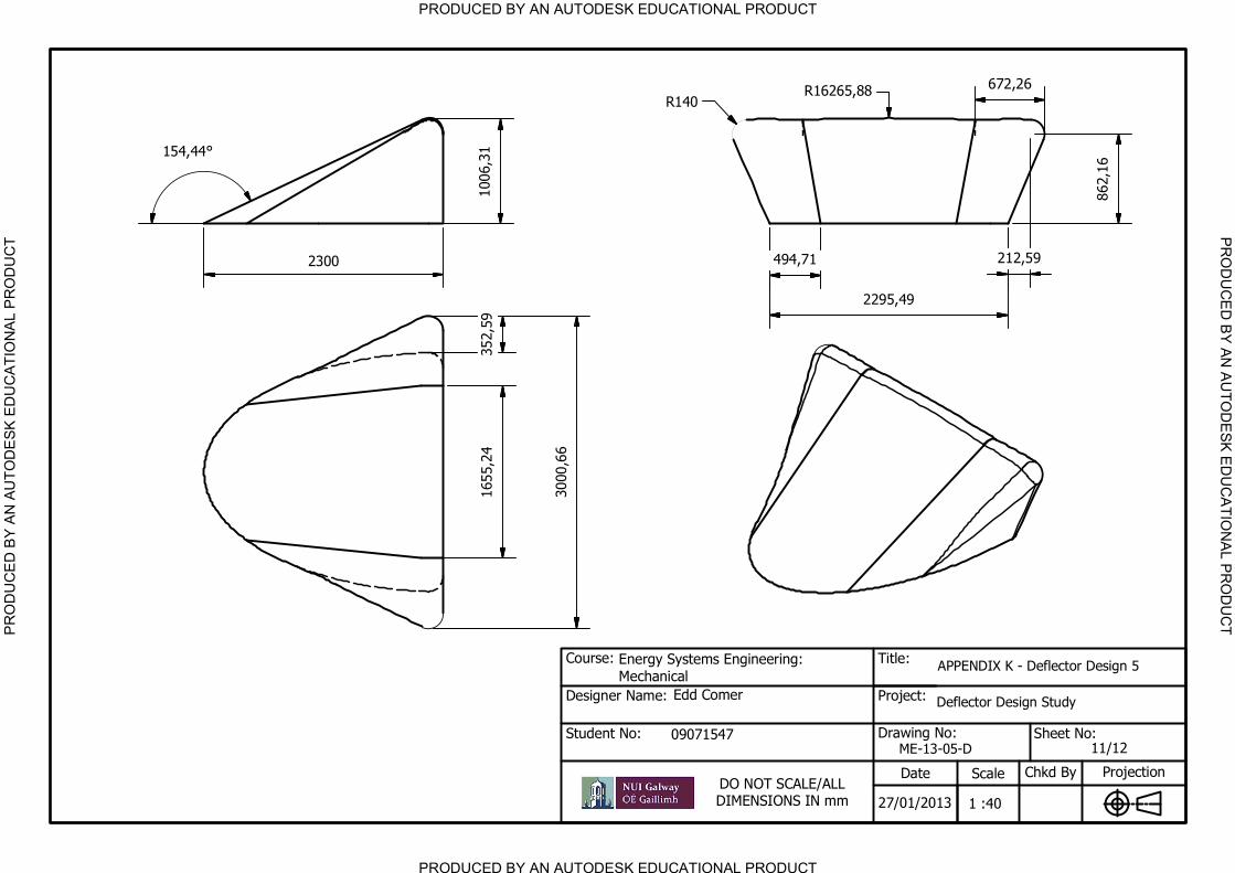
PRODUCED BY AN AUTODESK EDUCATIONAL PRODUCT

PRODUCED BY AN AUTODESK EDUCATIONAL PRODUCTP

RO

DU

CE

D B

Y A

N A

UT

OD

ES

K E

DU

CA

TIO

NA

L P

RO

DU

CT

PR

OD

UC

ED

B

Y A

N A

UT

OD

ES

K E

DU

CA

TIO

NA

L P

RO

DU

CT

Title:

Project:

Drawing No:

Date Scale

Projection

Designer Name:

Course:

Student No:

DO NOT SCALE/ALL

DIMENSIONS IN mm

Sheet No:

Chkd By

Energy Systems Engineering:

Mechanical

Edd Comer

09071547

APPENDIX K - Deflector Design 5

Deflector Design Study

ME-13-05-D

27/01/20131 :40

11/12

2300

1006,31

154,44°

1655,24

2295,49

R16265,88

R140

494,71

352,59

3000,66

672,26

212,59

862,16

PRODUCED BY AN AUTODESK EDUCATIONAL PRODUCT

PRODUCED BY AN AUTODESK EDUCATIONAL PRODUCTP

RO

DU

CE

D B

Y A

N A

UT

OD

ES

K E

DU

CA

TIO

NA

L P

RO

DU

CT

PR

OD

UC

ED

B

Y A

N A

UT

OD

ES

K E

DU

CA

TIO

NA

L P

RO

DU

CT

Title:

Project:

Drawing No:

Date Scale

Projection

Designer Name:

Course:

Student No:

DO NOT SCALE/ALL

DIMENSIONS IN mm

Sheet No:

Chkd By

Energy Systems Engineering:

Mechanical

Edd Comer

09071547

APPENDIX L: Model Truck Assembly

Model truck

ME-13-06-MT

27/01/20131 :120

12/12

100100

1250

300

700