HAL Id: hal-02997596https://hal.archives-ouvertes.fr/hal-02997596

Submitted on 10 Nov 2020

HAL is a multi-disciplinary open accessarchive for the deposit and dissemination of sci-entific research documents, whether they are pub-lished or not. The documents may come fromteaching and research institutions in France orabroad, or from public or private research centers.

L’archive ouverte pluridisciplinaire HAL, estdestinée au dépôt et à la diffusion de documentsscientifiques de niveau recherche, publiés ou non,émanant des établissements d’enseignement et derecherche français ou étrangers, des laboratoirespublics ou privés.

Efficient sizing and optimization of multirotor dronesbased on scaling laws and similarity models

Scott Delbecq, Marc Budinger, Aitor Ochotorena, Aurélien Reysset, FrançoisDefaÿ

To cite this version:Scott Delbecq, Marc Budinger, Aitor Ochotorena, Aurélien Reysset, François Defaÿ. Efficient sizingand optimization of multirotor drones based on scaling laws and similarity models. Aerospace Scienceand Technology, Elsevier, 2020, 102, pp.1-23. �10.1016/j.ast.2020.105873�. �hal-02997596�

�

�������������������������� �������������������������������������������������������

�������������������������������������

���������������������������������������������

������ �� ��� ���� ����� ��������� ����� �������� ���� ��� � ��� ���� ��������

���������������� �������������������������������������������������

�������������������������������������������������

����������������� ��

�

�

�

�

������������ ���

an author's https://oatao.univ-toulouse.fr/26691

https://doi.org/10.1016/j.ast.2020.105873

Delbecq, Scott and Budinger, Marc and Ochotorena, Aitor and Reysset, Aurélien and Defaÿ, François Efficient sizing

and optimization of multirotor drones based on scaling laws and similarity models. (2020) Aerospace Science and

Technology, 102. 1-23. ISSN 1270-9638

Efficient sizing and optimization of multirotor drones based on scaling

laws and similarity models

S. Delbecq a,∗, M. Budinger b, A. Ochotorena b, A. Reysset b, F. Defay a

a ISAE-SUPAERO, Université de Toulouse, 10 Avenue Edouard Belin, 31400 Toulouse, Franceb ICA, Université de Toulouse, UPS, INSA, ISAE-SUPAERO, MINES-ALBI, CNRS, 3 rue Caroline Aigle, 31400 Toulouse, France

o a b s t r a c t

Keywords:Multirotor dronesUAVDesign methodologySizingMonotonicity analysisMultidisciplinary Design Optimization

In contrast to the current overall aircraft design techniques, the design of multirotor vehicles generally consists of skill-based selection procedures or is based on pure empirical approaches. The application of a systemic approach provides better design performance and the possibility to rapidly assess the effect of changes in the requirements. This paper proposes a generic and efficient sizing methodology for electric multirotor vehicles which allows to optimize a configuration for different missions and requirements. Starting from a set of algebraic equations based on scaling laws and similarity models, the optimization problem representing the sizing can be formulated in many manners. The proposed methodology shows a significant reduction in the number of function evaluations in the optimization process due to a thorough suppression of inequality constraints when compared to initial problem formulation. The results are validated by comparison to characteristics of existing multirotors. In addition, performance predictions of these configurations are performed for different flight scenarios and payloads.

1. Introduction

Multirotor drones have become popular test-beds for Unmanned Aerial Vehicle (UAV) research and applications partly because of their great maneuverability and ability to execute complex movements. These capabilities have enabled them to be implemented in a wide range of both civil and military applications including surveillance, agriculture and other unprecedented purposes, such as automated package delivery or Personal Air Vehicles (PAVs). The competitiveness and search for new applications have encouraged industrials and academics to design lighter drones with improved flight times and efficiency.

Because UAVs are simple-to-use systems with a high level of support along with a good performance for most applications, a growth of customized and open solutions has taken place. To overcome some of their limitations, such as their reduced flight time, a set of tools must be developed to aid the design of customized solutions that can be tailored to a particular application.

Several approaches can be found in the literature to determine the most suitable design for the desired application. Popularly, among hobbyists, there is a practice of testing “motor+propeller” combinations and selecting the most appropriate one for a given purpose [1]. This approach is not generally adopted at a research or commercial level, due to its high cost or the high number of combinations required for a given application.

This process can be sped up by calculators such as eCalc [2] or Drive Calculator [3], based on the use of datatables, although the selection of components must be done individually, which is impractical when several models are to be sized, and when the payload scale factor differs from the typical market trend. Furthermore, these tools do not pay that much attention to the interrelations established between the rest of the components and consequently, do not give an optimal design of a Multirotor Aerial Vehicle (MRAV) as a whole and optimize its performance with respect to multidisciplinary objectives and constraints.

Holistic design approaches are subject to much interest for applications compelled by complex inter-relationships. Such approaches are mandatory for aerospace vehicles for instance fixed-wings [4], rotorcraft [5] or tilted-rotors [6]. To assist the designer, numerical methods have to be used to determine the best feasible configuration and can use different methods such as statistical-based [7] or optimization-based [8,9] techniques.

* Corresponding author.E-mail address: scott.delbecq@isae-supaero.fr (S. Delbecq).

https://doi.org/10.1016/j.ast.2020.105873

2 S. Delbecq et al. / Aerospace Science and Technology 102 (2020) 105873

In the literature, rotorcraft design and optimization methodologies are developed for different sub-systems to optimize the battery capacity [10], to select the optimum propulsion system components [11], or to design the controllers of miniature rotorcrafts [12]. There are conceptual layout optimization applicable to multiple multirotor drone systems [13] but their range of application and their surrogate models are based on small-scale drones.

In this sense, we consider necessary in this paper:

• To develop a systemic methodology to optimize the global design of the air vehicle, and for that, we will use Multidisciplinary Design Optimization (MDO) techniques.

• To formulate a reusable optimization code valid for a wide range of MRAVs based on scaling laws and surrogate models extracted from the dimensional analysis or the study of physical laws, as proposed in [14].

• To discuss about the mathematical and conflict resolution techniques to solve the possible singularities and complexity presented in an optimization code.

The global objective is to formulate in the most efficient way the basic architecture of the sizing of multirotor drones which would be extensible with the addition of higher fidelity models.

For this purpose, three major tasks are addressed in this paper: the implementation of a sizing procedure with special attention to the possible singularities found, a study of the design parameters for different mission characteristics and performance requirements, and the validation of obtained results over existing commercial MRAVs.

2. Preliminary design and sizing of multirotor drones

2.1. Design drivers and sizing scenarios

One of the biggest challenges in UAV industrial design is meeting required range and payload capacity for the various sizing scenarios. The sizing scenarios are part of the specification process and may include both transient and failure operating cases, such as a maximum rate of climb or resistance to a crash at a given height. These scenarios determine the main drone characteristics and the selection of mechanical and electronic components. The final overall design has to consider simultaneously transient and endurance criteria that may have impact on the components’ design drivers and system level parameters.

The diagram given in Fig. 1 shows the main system components, their main design drivers, and the main sizing equations for each scenario considered. Endurance scenarios, like hovering flight (referred to as HOV in the text) need to be taken into account for the selection of the battery endurance and the evaluation of the motor temperature rise. Extreme performance criteria, such as maximum transitory vertical acceleration (referred to as TO for Take-Off in the text) or maximum climb rate (referred to as CL in the text) are fundamental to determine the maximum rotational speed, maximum propeller torque, Electronic Speed Controller (ESC) corner power, battery voltage and power, and mechanical stress.

A list of the equations and models used in this paper can be found in Appendix A.

2.2. Components sizing models

Most of the design methodologies, despite the wide variety of implementations [20–22], are based on analytical expressions or catalog data regressions and benefit, as most continuous problems, of numerical optimization capabilities and high convergence performance. The paper [14] has shown how dimensional analysis and the Buckingham theorem can be used to estimate analytically the main characteristics of the components of a drone. A component characteristic y can be expressed as an algebraic function f of geometrical dimensions and physical/material properties:

y = f (L,d1,d2, ...︸ ︷︷ ︸geometric

, p1, p2, ...︸ ︷︷ ︸physical

) (1)

The application of the Buckingham theorem to the original Equation (1), with n parameters and u physical units (time, mass, length...), the equation can be rewritten with a reduced set of n − u dimensionless parameters called π numbers:

πy = f ′(πd1,πd2, ...,πp1,πp2, ...) (2)

where:

πy = yay · LaL∏

i

paii (3)

πdi = di

L(4)

πpi = Lapi,0∏

j

papi, j

i (5)

In the case where the dimensionless numbers πy and πdi can be assumed constant, such as respectively the one representing the magnetic saturation and the one representing the diameter-length ratio for the motor, then the function f can be approximated by using scaling laws or similarity models [23,24]. Otherwise, when data is available, regression models [25,26] are used such as for modeling the propeller performance or landing gear structural analysis. A detailed description of the hypotheses and methods associated with these sizing models of drone components can be found in [14].

S. Delbecq et al. / Aerospace Science and Technology 102 (2020) 105873 3

Fig. 1. Design drivers and sizing scenarios based on the following references: (propellers) [15]; (motors, battery and ESC) [16,17]; (frame) [18,19]. (For interpretation of the colors in the figure(s), the reader is referred to the web version of this article.)

2.3. Sizing procedure development

With progress of time, designers have established a sequence of well-defined calculations for multidisciplinary problems such as aircraft design and have applied optimization techniques to such engineering problem. These techniques, also known as Multidisciplinary Design Optimization (MDO), are useful to study the complete aircraft that involves couplings between different subsystems.

The resolution of a MDO problem requires to address two main aspects:

• structuring the architecture of the MDO problem by choosing the computational sequence and solving the coupling variables. For this purpose, the computational process can be represented by graphs such as the N2 diagram [23] or the eXtended Design Struc-ture Matrix (XDSM) [27]. The resolution of the multidisciplinary couplings can be achieved using different distributed or monolithic MDO formulations such as the MultiDisciplinary Feasible (MDF) of the Individual Discipline Feasible (IDF). Here a monolithic Normal-ized Variable Hybrid (NVH) formulation is used as it is fast and robust to scale-change due to the usage of inequality constraints, a small dimension consistency design variable and a reduced number of constraints and design variables [28]. However, it does not guarantee system consistency when the optimizer fails when compared to the MDF. Hybrid approaches, derived from IDF, are partic-ularly interesting here because of the reasonable number of variables and constraints to be managed as they keep the feed-forward computational sequence [29],

• implementing optimization algorithms to compute the best final result with far-fewer case evaluations. The design of a MRAV is considered here as a standard constrained optimization problem [30], where a single objective (e.g. maximum take-off weight) is minimized with respect design variables (e.g. battery capacity) and subject to constraints (e.g. motor maximum torque).

The following sections will show how to structure this optimization problem through a systemic sizing procedure in order to facilitate the work of the optimization algorithms.

3. Sizing procedure definition

The sizing procedure is the sequence of calculation steps to be carried out to define the size and feature of the drone components. This procedure can be represented as an algorithm or flowchart as shown in Fig. 2. The XDSM diagram provides a visual summary of

4 S. Delbecq et al. / Aerospace Science and Technology 102 (2020) 105873

Fig. 2. Initial XDSM diagram for multirotor drone optimization.

Table 1Methodology summary.

Process Methods & tools References

Step 1: Define a system of algebraic equations S based on estimation models and simulation models subject to inequality constraints

Analytical models, Scaling laws, Datasheet regression [24,34,14]

Step 2: Reduce (when possible) the number of inequality constraints First Monotonicity Principle (MP1) Section 3.2.1, [35]

Step 3: Build undirected bipartite graph/design graph from S , identify Strongly Connected Components (SCC) and solve them by implementing the NVH formulation

Design graphs, Symbolic computation, Graph algorithms Section 3.3, Section 3.4, [36,37,34,28]

Step 4: Perform a matching and ordering of the modified system and generate the sizing procedure

Graph algorithms, Symbolic computation [36,37,34]

the efficiency of the ordering and is useful to visualize the models involved and the shared variables. Once the required thrust for every mission is estimated from an initial guess of the total drone mass, propeller torque and speed characteristics are estimated. Based on these values and the application of scaling laws, motor parameters are calculated and subsequently, the ESC, battery and frame parameters. This enables determine the contribution of components mass to the total mass of the drone. However, this total mass is required to determine hover and take-off thrust thus leading to an algebraic loop which has to be solved using an MDO strategy [31].

Feed-back loops have to be avoided as much as possible in the calculation procedure, since they have significant impact on the com-putational effectiveness [32]. For the remaining loops, the NVH formulation approach is implemented by introducing dedicated additional constraints and design variables in an optimization process in order to solve the multidisciplinary couplings such as the mass loop in Fig. 2 [33,28].

3.1. Sizing methodology

Solving a design optimization problem requires to follow an orderly methodology. Defining the steps in a structured way helps to incorporate new design variables in the optimization routine and serves to orientate the equations towards a solution. The proposed design optimization methodology can be summarized in Table 1.

Once the equations are defined, there are three manners of treating the inequality constraints:

A) consider all the inequality constraints found in the problem as inactive1 and rely entirely on the solver to find a solution. In this case the process skips steps 2 and 3.

B) identify active and inactive constraints after application of MP1, transform the critical2 active3 inequalities to equalities and let the remaining inequalities, which boundedness behavior is undetermined, be solved by the solver. This is the approach proposed by Papalambros and Wilde in [35]. In this case the process skips step 3.

1 An inequality constraint gi(x) ≤ 0 is said to be inactive at a design point xk if it has negative value at that point (i.e., gi(xk) < 0) [38].2 When there is only one constraint bounding a certain variable positively and finitely [35].3 An inequality constraint gi(x) ≤ 0 is said to be active at a design point xk if it is satisfied as an equality at that point (i.e., gi(xk) = 0) [38].

S. Delbecq et al. / Aerospace Science and Technology 102 (2020) 105873 5

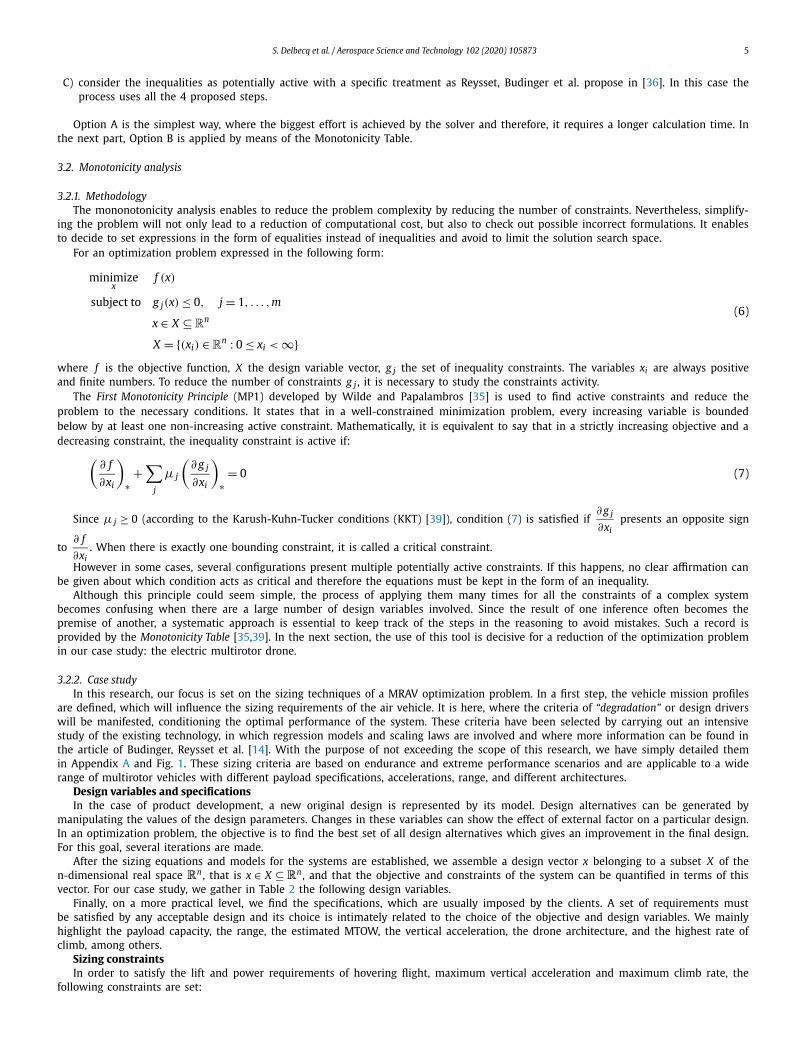
C) consider the inequalities as potentially active with a specific treatment as Reysset, Budinger et al. propose in [36]. In this case the process uses all the 4 proposed steps.

Option A is the simplest way, where the biggest effort is achieved by the solver and therefore, it requires a longer calculation time. In the next part, Option B is applied by means of the Monotonicity Table.

3.2. Monotonicity analysis

3.2.1. MethodologyThe mononotonicity analysis enables to reduce the problem complexity by reducing the number of constraints. Nevertheless, simplify-

ing the problem will not only lead to a reduction of computational cost, but also to check out possible incorrect formulations. It enables to decide to set expressions in the form of equalities instead of inequalities and avoid to limit the solution search space.

For an optimization problem expressed in the following form:

minimizex

f (x)

subject to g j(x) ≤ 0, j = 1, . . . ,m

x ∈ X ⊆ Rn

X = {(xi) ∈Rn : 0 ≤ xi < ∞}

(6)

where f is the objective function, X the design variable vector, g j the set of inequality constraints. The variables xi are always positive and finite numbers. To reduce the number of constraints g j , it is necessary to study the constraints activity.

The First Monotonicity Principle (MP1) developed by Wilde and Papalambros [35] is used to find active constraints and reduce the problem to the necessary conditions. It states that in a well-constrained minimization problem, every increasing variable is bounded below by at least one non-increasing active constraint. Mathematically, it is equivalent to say that in a strictly increasing objective and a decreasing constraint, the inequality constraint is active if:(

∂ f

∂xi

)∗+

∑j

μ j

(∂ g j

∂xi

)∗= 0 (7)

Since μ j ≥ 0 (according to the Karush-Kuhn-Tucker conditions (KKT) [39]), condition (7) is satisfied if ∂ g j

∂xipresents an opposite sign

to ∂ f

∂xi. When there is exactly one bounding constraint, it is called a critical constraint.

However in some cases, several configurations present multiple potentially active constraints. If this happens, no clear affirmation can be given about which condition acts as critical and therefore the equations must be kept in the form of an inequality.

Although this principle could seem simple, the process of applying them many times for all the constraints of a complex system becomes confusing when there are a large number of design variables involved. Since the result of one inference often becomes the premise of another, a systematic approach is essential to keep track of the steps in the reasoning to avoid mistakes. Such a record is provided by the Monotonicity Table [35,39]. In the next section, the use of this tool is decisive for a reduction of the optimization problem in our case study: the electric multirotor drone.

3.2.2. Case studyIn this research, our focus is set on the sizing techniques of a MRAV optimization problem. In a first step, the vehicle mission profiles

are defined, which will influence the sizing requirements of the air vehicle. It is here, where the criteria of “degradation” or design drivers will be manifested, conditioning the optimal performance of the system. These criteria have been selected by carrying out an intensive study of the existing technology, in which regression models and scaling laws are involved and where more information can be found in the article of Budinger, Reysset et al. [14]. With the purpose of not exceeding the scope of this research, we have simply detailed them in Appendix A and Fig. 1. These sizing criteria are based on endurance and extreme performance scenarios and are applicable to a wide range of multirotor vehicles with different payload specifications, accelerations, range, and different architectures.

Design variables and specificationsIn the case of product development, a new original design is represented by its model. Design alternatives can be generated by

manipulating the values of the design parameters. Changes in these variables can show the effect of external factor on a particular design. In an optimization problem, the objective is to find the best set of all design alternatives which gives an improvement in the final design. For this goal, several iterations are made.

After the sizing equations and models for the systems are established, we assemble a design vector x belonging to a subset X of the n-dimensional real space Rn , that is x ∈ X ⊆ Rn , and that the objective and constraints of the system can be quantified in terms of this vector. For our case study, we gather in Table 2 the following design variables.

Finally, on a more practical level, we find the specifications, which are usually imposed by the clients. A set of requirements must be satisfied by any acceptable design and its choice is intimately related to the choice of the objective and design variables. We mainly highlight the payload capacity, the range, the estimated MTOW, the vertical acceleration, the drone architecture, and the highest rate of climb, among others.

Sizing constraintsIn order to satisfy the lift and power requirements of hovering flight, maximum vertical acceleration and maximum climb rate, the

following constraints are set:

6 S. Delbecq et al. / Aerospace Science and Technology 102 (2020) 105873

Table 2Model-dependent design variables.

Vars. Description System Units

β Ratio pitch-to-diameter Propeller [–]nD Rotational speed per diameter for take-off Propeller [Hz · m]J Advance ratio Propeller [–]

Ubat Battery voltage Battery [V]Cbat Battery capacity Battery [A · s]

Tmot Required nominal motor torque Motor [N · m]KT Motor constant Motor

[N·m

A

]P E SC ESC Power ESC [W]

Larm Arm length Frame [m]Dout Outer arm diameter Frame [m]k f rame Ratio inner-to-outer arm diameter Frame [–]Mtotal Initial guess for MTOW Global [kg]

• Hovering flight:– Nominal torque, Tmot , will be equal to or greater than the motor torque in hovering flight, Tmot,hov (g1).

• Transitory vertical acceleration (Take-Off)– Maximum torque, Tmax,mot , will be equal to or higher than the motor torque under the conditions of maximum transient vertical

acceleration, Tmot,to (g2).– Voltage provided by the battery, Ubat , will satisfy the motor voltage demand under the conditions of maximum transient vertical

acceleration, Umot,to (g3).– Voltage provided by the battery, Ubat , will satisfy the ESC voltage demand under conditions of maximum transient vertical acceler-

ation, U E SC (g4).– Maximum battery power, Pbat , will satisfy the motors power demand under the conditions of maximum transient vertical acceler-

ation, Pmot,to,total (g5).– Power provided by the ESC, P E SC , will satisfy the power demand under the conditions of maximum transient vertical acceleration,

P E SC,to (g6).– Product of speed and diameter under the conditions of maximum transient vertical acceleration, nD , will not overpass the speed

limit provided by the propeller manufacturer, nDmax (g7).– No mechanical load greater than the one permitted by the arm material, σmax , shall be exceeded under the conditions of maximum

transient vertical acceleration (g8).• Maximum climb rate

– Maximum torque, Tmax,mot , will be equal to or higher than the propeller torque under the conditions of highest climbing rate, Tmot,cl(g9).

– Voltage provided by the battery, Ubat , will satisfy the motor voltage demand under the conditions of highest climbing rate, Umot,cl(g10).

– Voltage provided by the battery, Ubat , will satisfy the ESC voltage demand under the conditions of highest climbing rate, U E SC (g3).– Maximum battery power, Pbat , will satisfy the motors power demand under the conditions of highest climbing rate, Pmot,cl,total

(g11).– Power provided by the ESC, P E SC , will satisfy the power demand under the conditions of highest climbing rate, P E SC,cl (g12).– Product of speed and diameter under the conditions of highest climbing rate, npro,cl D pro , will not overpass the speed limit provided

by the propeller manufacturer, nDmax (g13).– Since the implementation of equality constraints may engender numerical difficulties for the optimization algorithm [35], an ap-

proach to solve the algebraic loop for the equation of vertical climb rate:

V cl − Jnpro,cl D pro = 0 (8)

is to break out the expression into two inequalities (g14, g15) resulting into an absolute error of 5%.• Geometry

– The arms will have a minimum length, Larm , such that the propellers do not overlap for a regular motor layout (g16).• Global system constraints

To the previous constraints, two necessary conditions are included to bring coherence to the problem. Depending on the objective:– To minimize the mass, the calculated endurance (thov ) will converge to the estimated flight time (th).– To maximize the range, the estimated Maximum Take-Off Weight (MTOW) will converge to the calculated final mass (Mtotal, f inal).In addition, for both cases, the final mass (Mtotal, f inal) will converge with the initial guess (Mtotal).

Objective functionOn the basis of the XDSM diagram developed in Fig. 2, if the proposed design objective is the minimization of the final total mass, the

total mass can be extressed as the sum of the different component masses:

f : Mtotal, f inal = Mpro + Mmot + Mbat + ME SC + M f rame (9)

If this expression is broken down into minimum design variables, we can see how we obtain a complex mathematical expression dependent on the different design variables:

S. Delbecq et al. / Aerospace Science and Technology 102 (2020) 105873 7

Table 3Application of First Monotonicity Principle to identify active constraints. The expression highlighted in yellow is a critical expression and can be transformed into equality with respect to the variable of the column with a red circle, because the sign of its first derivative is the only opposite to the sign of the first derivative of the objective.

Mtotal nD Tmot Ktmot P E SC Ubat Cbat β J k f rame Larm Dout

Objective f + − + + − − + +H g1 : Tmot,hov − Tmot ≤ 0 + − −TAKE-OFF g2 : Tmot,to − Tmot,max ≤ 0 + − −

g3 : Umot,to − Ubat ≤ 0 − + − +g4 : U E SC − Ubat ≤ 0 + −g5 : Pmot,to,total − Pbat ≤ 0 + − −g6 : P E SC,to − P E SC ≤ 0 − +g7 : nD − nDmax ≤ 0 +g8 : Fmax,arm ·Larm

π ·(

D4out −D4

in

)32·Dout

− σmax ≤ 0 + + + −©MAX CLIMB g9 : Tmot,cl − Tmot,max ≤ 0 + − − + +

g10 : Umot,cl − Ubat ≤ 0 − + − + +g11 : Pmot,cl,total − Pbat ≤ 0 + − + +g12 : P E SC,cl − P E SC ≤ 0 − +g13 : npro,cl D pro − nDmax ≤ 0 − + +g14 : V cl − Jnpro,cl D pro ≤ 0 + − −g15 : Jnpro,cl D pro − V cl ≤ 0.05 − + +

GEO g16 : D pro

2 · sin( πNarm )

− Larm ≤ 0 + − − −©

Mtotal = f (Mtotal, β,nD, Ubat , Tmot, KT , Cbat, P E SC , Larm, Dout,k f rame, J ) (10)

Next, a monotonicity analysis of the objective and constraints functions is carried out, based on the models given in the appendixes, over the different design variables displayed in Table 2. In a general way, the Monotonicity Table includes a column for each variable and a row for the objective function and each constraint. The global system constraints are excepted of this analysis because they represent the necessary conditions for the proper performance of the optimization problem. The elements of the resulting matrix indicate the incidence and monotonicity of each variable in each constraint.

Each column records a variable and the constraints can bound whether from above (also known as strictly monotone increasing) or from below (strictly monotone decreasing).

Table 3 shows the arrangement of columns and rows. The top row contains the monotonicity of the objective function, with the variables heading the columns indicating ‘+’ for strictly monotone increasing and ‘−’ for strictly monotone decreasing. Monotonicities for the constraints are given in the matrix to the right of the constraints column. For the constraints, if the condition of critical constraint is met, such expression can be written as equality.

The results show a multiple activity of the constraints with respect to the objective function. Some of these constraints are critical and others are potentially active. To cite some examples of potentially active constraints: the objective function is bounded above with respect to N D , by g7, g13 and g15; and below with respect to Tmot by g1, g2, g3.g5, g9, g10 and g11. Since the sign of the variable is opposite to that of the objective function in several constraints, no evident statement can be given and in that case, these constraints potentially active, will be left here as inequalities. These critical constraints are detected:

g8(M+total,k+

f rame, L+arm, D−

out) critical w.r.t Dout → Dout = 3

√32 · Fmax,arm · Larm

π · σmax · (1 − Din/Dout)(11)

g16(M+total,nD−, β−, L−

arm) critical w.r.t Larm → Larm = D pro

2 · sin( πNarm )

(12)

The number of inequality constraints has been successfully reduced from sixteen to fourteen. In the following sub-section, Algorithm C addresses the rest of the potentially active inequalities. Through the construction of Design Graphs [36] it is possible to establish relation-ships between parameters and to propose alternative resolution strategies.

3.3. Under- and over-constrained singularities

The complexity of a design problem can be significantly reduced through the application of two methods. To start, the First Mono-tonicity Principle, a generalist approach based on a mathematical study of the monotonicity system’s equations (algorithm B and C) can be used. Then, the computational process can be represented by design graphs and the use of graph algorithms enable to detect possible singularities which may require additional computational effort. The method for solving these are presented and used only by algorithm C.

The objective of design graphs is to graphically highlight the main singularities when building a sizing code. The ultimate goal is to sequence explicitly a set of equations. The initial set of equations can be: under-constrained, over-constrained or contain algebraic loops. The graph edges are oriented with an arrow when the vertice are known and non-oriented when the orientation of the problem remains to be determined. To establish the design graphs, two layers of knowledge are distinguished. A system layer, which links the parameters of multiple components with the specifications for any sizing scenario. A component layer, which links parameters with equations based on the own characteristics of the component and are only applied for a specific component used in the design. Models, design equations and design variables are framed in a rectangle, while the specific parameters and characteristics are in circles.

8 S. Delbecq et al. / Aerospace Science and Technology 102 (2020) 105873

Fig. 3. Design Graph for a propeller selection (before strategy).

Fig. 4. Design Graph for a propeller selection (after strategy).

3.3.1. Under-constrained singularitySizing issue: Equation subset has an infinity of solutions due to the excess of parameters.Example: For a given payload capacity, the maximum thrust is calculated according to Equation (C.1). But the first problem faced here

is:

CT?= f (Fmax,ρair,n, D pro)

for which only Fmax and ρair are known (Fig. 3).Method: Substitution of unknown parameters by normalized sizing coefficients. The use of standardized coefficients as design variables

will ensure the validity of a design range for a wide spectrum of specifications.Once the regression model for the thrust coefficient CT is obtained as a function of pitch

D pro(new design variable), the range of the thrust

coefficient can be estimated. On the other hand, the CT equation can be reformulated if the RPM limit is taken into account this way:

(nD) ≤ (nD)max → (nD) · kN D = (nD)max

with (nD)max dependent on the propeller technology and kN D as a degree of freedom within the range [0, 1]. This helps to continue the computation process by bounding a variable with a reduced range.4

CT = Fmax

ρ · (nD)2 · D2pro

= Fmax

ρ ·(

nDmaxkN D

)2 · D2pro

Once the modification is done inside the equation, the propeller diameter D pro can be calculated. In Fig. 4, the orientation of the problem is depicted. This diagram should be understood by the end of the explanation. After a certain number of iterations, the optimizer will find the right value of kN D that satisfies the constraint and thus the system requirements.

A similar case is found in the frame sizing as shown in Fig. 5.Equation (11) depends on the known parameter Fmax and on the already calculated Larm . Dout and Din remain unknowns.A way to solve this under-determined situation consists of expressing Din as a function of Dout :

Din = k f rame · Dout (13)

where the aspect ratio k f rame remains between (0,1).

4 Similarly, n or D could have been imposed instead of kN D but in this case the ranges to explore are much wider and depend strongly on the specifications of the drone (small or large carrier).

S. Delbecq et al. / Aerospace Science and Technology 102 (2020) 105873 9

Fig. 5. Design Graph for the frame selection (in red underconstraint).

Fig. 6. Overconstrained singularity for the motor selection.

3.3.2. Over-constrained singularitySizing issue: Different equations yield the same output.Example: The motor sizing sets out three equations with two undetermined parameters (Tmot and Tmax,mot ):

Tmax,mot ≥ T pro,to (14)

Tmot ≥ T pro,hov (15)

Tmax,mot = Tmax,mot,ref · Tmot

Tmot,ref(16)

The reference component data Tmax,mot,ref and Tmot,ref are available as well as the propeller scenario T pro,hov and T pro,to . It is high-lighted through the Design Graph shown at Fig. 6, that the problem has in fact three equations with two over-constrained parameters.

Method: Shift some of the equations to the inequality constraints and introduce degrees of freedom to represent the equalities.To obtain a non-singular problem, one of the three equations must be removed, by placing one of the inequalities in the optimization

constraints, like Equation (14) for example. Then, Equation (15) is transformed to an equality by introducing a degree of freedom kmot :

Tmot = kmot · T pro,hov (17)

with kmot as a variable input within the range [1,∞). This formulation allows to have a design variable whose lower bound is independent of the application specification.

Another example is found for the calculation of maximum power provided by the battery (Fig. 7). The battery must provide enough power to operate for the maximum transient modes (climb and take-off). Here, a problem with three equations and one undetermined parameter (Pmax,bat ) can be found:

Pmax,bat = Ubat · Imax (18)

Pmax,bat ≥ Umot,to Imot,to Npro

ηesc(19)

Pmax,bat ≥ Umot,cl Imot,cl Npro

ηesc(20)

Since three equations yield the same output, the two inequalities are placed in the optimization constraints.

3.4. Resolution of algebraic loops

Sizing issue: Circular dependency between inputs and outputs.Example: This problem is found during the motor selection:

Umot,to = Rmot · Ito + KT ,mot · �mot,to (21)

where only Umot and �mot,to are known. An algebraic loop appears here since K T is necessary to determine the motor resistance R:

10 S. Delbecq et al. / Aerospace Science and Technology 102 (2020) 105873

Fig. 7. Overconstrained singularity for the battery selection.

Fig. 8. Design Graph for a motor selection (in red algebraic loop).

Rmot = Rmot,ref

(KT ,mot

KT ,mot,ref

)2 (Tmot

Tmot,ref

)−5/3.5

(22)

Method: By removing the term corresponding to the imperfection in the Equation (21), i.e. the product R · Ito , the algebraic loop is broken. A minimum oversizing coefficient, kspeeedmot ≥ 1, is introduced to compensate the missing term in the initial equation. The initial inequality is reintroduced in the constraints to ensure the consistency.

Umot,to = kspeedmot · KT · �mot,to (23)

From this new expression, the value of KT is obtained and with this, we calculate the motor resistance R substituting the value of the motor constant in Equation (22).

Finally, a constraint is set up to validate the above simplification:

Ubat ≥ Umot,to (24)

This process is illustrated in Fig. 8 where the algebraic loop is marked with red arrows.Another example is found for the initial mass estimation. To launch the procedure, it is assumed that the initial guess for MTOW,

Mtotal , is a multiple of the known payload Mload .

Mtotal = kM · Mload (25)

After several iterations, the final mass, Mtotal, f inal calculated as sum of the different components must converge to this initial guess Mtotal . This is expressed by the following inequality:

Mtotal ≥ Mtotal, f inal (26)

This condition is added to the global constraints, so that both results tend to a unique solution.

4. Overall sizing optimization

4.1. Summary of the sizing codes

Once the different sizing equations and expressions have been formulated and oriented, they are integrated into an optimization code to calculate the optimal design of the systems for a specific objective. One of the goals of this paper is to demonstrate how the application of the previous strategies may lead to a reduction of the problem complexity and the resolution time for the same or a better solution. Thus, three algorithms are developed which are based on the different modifications proposed:

S. Delbecq et al. / Aerospace Science and Technology 102 (2020) 105873 11

Fig. 9. N2 diagram for solving the optimization problem using algorithm A. Modifications carried out by algorithms B and C over algorithm A are highlighted with colors.

• Algorithm A based on the initial constraints and design variables proposed in Table 2 and section 3.2.2. This algorithm applies Step 1 and 4 of the methodology shown in Table 1.

• Algorithm B after having reduced the number of inequality constraints through application of MP1 proposed in Table 3. This algorithm applies Step 1, 2 and 4 of the methodology shown in Table 1.

• Algorithm C with the application of MP1 and substitution of the model-dependent design variables by sizing coefficients valid for a wide range of models as suggested in section 3.3 and section 3.4. This algorithm applies Step 1, 2, 3 and 4 of the methodology shown in Table 1.

The optimizer used is a heuristic method from the SciPy Python library: the differential evolution. This sizing process is illustrated in Fig. 9 through the XDSM tool to describe the interfaces among components of a complex system.

This diagram, which follows the same sizing procedure as explained in section 3, highlights the different modifications made on the basis of the initial algorithm A. For the algorithm B, as a result of a monotonicity analysis, the inequality constraints of the frame are eliminated, while for algorithm C, design variables are replaced by standardized coefficients and further inequality constraints are removed.

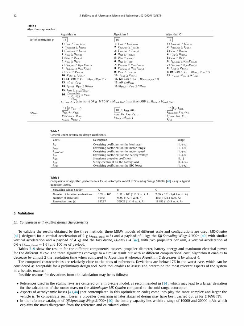
A summary of the different design approaches of each algorithm is shown in Table 4. If we recap the standard formulation of an optimization problem in Equation (6), we can see that the total number of design constraints (defined as m) and design variables (defined as n) corresponds to the framed value of the first and second row of Table 4 for each algorithm, respectively. With the application of the Algorithm C we manage to express the problem in general normalized coefficients. The range and description of these coefficients are shown in Table 5.

The use of normalized sizing coefficients (around 1 or one bound equal to 1) as optimization variables enables to have a generic sizing code since the optimization limits do not longer depend on the size of the vehicle. Although the implementation is somehow complex and needs a good understanding of the system to replace equations, the use of design graphs and the algorithms presented in [36,34]makes this step easier. The interesting performances, highlighted by the number of iterations, and reduced resolution time in Table 6 of this Normalized Variable Hybrid formulation is also benchmarked in terms of computational cost and robustness versus other monolithic MDO formulations in [28].

12 S. Delbecq et al. / Aerospace Science and Technology 102 (2020) 105873

Table 4Algorithms approaches.

Algorithm A Algorithm B Algorithm C

Set of constraints gi 181 : Tmot ≥ Tmot,hover

2 : Tmax,mot ≥ Tmot,to

3 : Tmax,mot ≥ Tmot,cl

4 : Ubat ≥ Umot,to

5 : Ubat ≥ Umot,cl

6 : Ubat ≥ U E SC

7 : Pbat,max ≥ N pro Pmot,to

8 : Pbat,max ≥ N pro Pmot,cl

9 : P E SC ≥ P E SC,to

10 : P E SC ≥ P E SC,cl

11, 12 : 0.05 ≥ V cl − Jnpro,cl D pro ≥ 013 : nD ≤ nDmax

14 : npro,cl · D pro ≤ N Dmax

15 : Larm ≥ D pro2·sin(π/Narm)

16 : Fmax,arm ·Larm

π ·(

D4out −D4

in

)32·Dout

≤ σmax

161 : Tmot ≥ Tmot,hover

2 : Tmax,mot ≥ Tmot,to

3 : Tmax,mot ≥ Tmot,cl

4 : Ubat ≥ Umot,to

5 : Ubat ≥ Umot,cl

6 : Ubat ≥ U E SC

7 : Pbat,max ≥ N pro Pmot,to

8 : Pbat,max ≥ N pro Pmot,cl

9 : P E SC ≥ P E SC,to

10 : P E SC ≥ P E SC,cl

11, 12 : 0.05 ≥ V cl − Jnpro,cl D pro ≥ 013 : nD ≤ nDmax

14 : npro,cl · D pro ≤ N Dmax

131 : Tmax,mot ≥ Tmot,to

2 : Tmax,mot ≥ Tmot,cl

3 : Ubat ≥ Umot,to

4 : Ubat ≥ Umot,cl

5 : Ubat ≥ U E SC

6 : Pbat,max ≥ N pro Pmot,to

7 : Pbat,max ≥ N pro Pmot,cl

8 : P E SC ≥ P E SC,cl

9, 10 : 0.05 ≥ V cl − Jnpro,cl D pro ≥ 011 : npro,cl · D pro ≤ N Dmax

g : thov ≥ th (min mass) OR g : MT O W ≥ Mtotal, f inal (max time) AND g : Mtotal ≥ Mtotal, f inal

D.Vars.

12 β, Tmot ,nD,

Ubat , KT , Cbat ,

P E SC , Larm, Dout ,

k f rame, Mtotal, J

10 β, Tmot ,nD,

Ubat , KT , Cbat , P E SC ,

k f rame, Mtotal, J

10 kM ,kmot ,

kspeed,mot ,kvb,kN D ,

k f rame,kMb, β, J ,kE SC

Table 5General under-/oversizing design coefficients.

Coefs. Description Range

kM Oversizing coefficient on the load mass [1,+∞)

kmot Oversizing coefficient on the motor torque [1,+∞)

kspeed,mot Oversizing coefficient on the motor speed [1,+∞)

kvb Oversizing coefficient for the battery voltage [1,+∞)

kN D Slowdown propeller coefficient (0,1]kMb Sizing coefficient on the battery load (0,+∞)

kE SC Oversizing coefficient on the ESC Power [1,+∞)

Table 6Comparison of algorithm performances for an octocopter model of Spreading Wings S1000+ [40] using a typical quadcore laptop.

Spreading wings S1000+ A B C

Number of function evaluations 3.74 × 106 1.51 × 106 (1/2.5 w.r.t. A) 7.69 × 105 (1/4.9 w.r.t. A)Number of iterations 19191 9090 (1/2.1 w.r.t. A) 4659 (1/4.1 w.r.t. A)Resolution time (s) 637.87 399.22 (1/1.6 w.r.t. A) 181.87 (1/3.5 w.r.t. A)

5. Validation

5.1. Comparison with existing drones characteristics

To validate the results obtained by the three methods, three MRAV models of different scale and configurations are used: MK-Quadro[41], designed for a vertical acceleration of 2 g (kmax,thrust = 3) and a payload of 1 kg; the DJI Spreading Wings S1000+ [40] with similar vertical acceleration and a payload of 4 kg and the taxi drone, EHANG 184 [42], with two propellers per arm, a vertical acceleration of 0.6 g (kmax,thrust = 1.6) and 100 kg of payload.

Tables 7–9 show the results for the different components’ masses, propeller diameter, battery energy and maximum electrical power for the different MRAV. The three algorithms converge to a similar result but with at different computational cost. Algorithm B enables to decrease by almost 2 the resolution time when compared to Algorithm A whereas Algorithm C decreases it by almost 4.

The computed characteristics are relatively close to the ones of references. Deviations are below 17% in the worst case, which can be considered as acceptable for a preliminary design tool. Such tool enables to assess and determine the most relevant aspects of the system in a holistic manner.

Possible reasons for deviations from the calculation may be as follows:

• References used in the scaling laws are centered on a mid-scale model, as recommended in [14], which may lead to a larger deviation for the calculation of the motor mass on the Mikrokopter MK-Quadro compared to the mid-range octocopter.

• Aspects of aerodynamic losses [43,44] (not contemplated in this optimization code) come into play the more complex and larger the vehicle is. To compensate such losses, a propeller oversizing in later stages of design may have been carried out as for EHANG 184.

• In the reference catalogue of DJI Spreading Wings S1000+ [40] the battery capacity lies within a range of 10000 and 20000 mAh, which explains the mass divergence from the reference and calculated values.

S. Delbecq et al. / Aerospace Science and Technology 102 (2020) 105873 13

• One possible explanation to explain the overall divergence from the reference and calculated values of the battery properties, may be that batteries could be designed to provide longer flight times than indicated for safety reasons.

• Additional weights (antenna, GPS, receivers, flight controller, ...) may not be included in the reference catalogues.

Quadcopter: Mikrokopter MK-Quadro

MK QUADRO. Source: [41].

⎧⎪⎨⎪⎩

Payload: 1.0 kg kmax,thrust : 3Number of arms: 4 Number of propeller per arm 1Climb speed: 10 m/s Drag coefficient: 1.3Endurance: 15 min Top surface: 0.045 m2

⎫⎪⎬⎪⎭

Table 7Comparison of results for the different algorithms applied to MK-Quadro.

Alg. A Alg. B Alg. C Reference Rel. Error (%)

Total mass (g) 1642 1409 +16.53Battery Mass (g) 353 329 +7.29Motor Mass (g) 47 54 −12.96Diameter Prop (m) 0.25 0.25 0.00Energy (W.h) 53.95 48.84 +10.46Max Power (W) 172.99 175 −1.14

Octocopter: DJI Spreading Wings S1000+

Spreading Wings S1000+. Source: [40].

⎧⎪⎨⎪⎩

Payload: 4 kg kmax,thrust : 3Number of arms: 8 Number of propeller per arm 1Climb speed: 6 m/s Drag coefficient: 1.3Endurance: 18 min Top surface: 0.09 m2

⎫⎪⎬⎪⎭

14 S. Delbecq et al. / Aerospace Science and Technology 102 (2020) 105873

Table 8Comparison of results for the different algorithms applied to Spreading Wings S1000+.

Alg. A Alg. B Alg. C Reference Rel. Error (%)

Total mass (g) 8513 9500 −10.38Battery Mass (g) 2133 1932 +10.41Motor Mass (g) 160 158 +1.26Diameter Prop (m) 0.40 0.38 +5.26Energy (W.h) 326.20 333 −2.04Max Power (W) 448.54 500 −10.29

Coaxial propellers setup: EHANG 184

Ehang 184 autonomous aerial vehicle: Source: [42].

⎧⎪⎪⎨⎪⎪⎩

Payload: 100 kg kmax,thrust : 1.6Number of arms: 4 Number of propeller per arm 2Climb speed: 5 m/s Drag coefficient: 1.3Endurance: 22 min Top surface: 2.09 m2

⎫⎪⎪⎬⎪⎪⎭

Table 9Comparison of results for the different algorithms applied to EHANG 184.

Alg. A Alg. B Alg. C Reference Rel. Error (%)

Total mass (kg) 404.18 360 +12.5Diameter Prop (m) 2.00 1.7 +17.65Max Power (W) 11358.27 13250 −14.28

6. Design exploration

Within the multidisciplinary design, components adapt their performance and characteristics to meet the different design objectives. In this part, we will focus on some of these variations to satisfy the objectives of maximizing the mission time and minimizing the mass.

6.1. Effect of the acceleration requirement

In Fig. 10, we show an evolution of the flight time of an octocopter as a function of the vertical acceleration and its take-off weight. The diagram shows how a higher acceleration implies a reduction of the flight time. This reduction is due to the increase of motor weight in order to provide the required torque. This trend shown to be more pronounced as a certain acceleration value is exceeded, as can be seen for a large drone for values beyond 1.5.

6.2. Effect of increased range on component size

As depicted in Fig. 11, the air vehicle size increases exponentially as a longer flight time is required. An increase in range implies more electrical power required by the different components and also a larger design, which can be reflected in the growth of the propeller diameter.

S. Delbecq et al. / Aerospace Science and Technology 102 (2020) 105873 15

Fig. 10. Evolution of flight times for an octocopter with single motor setup with different vertical accelerations and loads.

Fig. 11. Evolution of the components’masses and propeller diameter growth curve with respect to the flight time for a quadcopter of MTOW of 30 kg.

Fig. 12. Effect of the gearbox on the evolution of the components’ masses (for a given endurance of 15 min).

6.3. Effect of a gearbox on system mass reduction

In the following part, it will be shown how the motor mass can be greatly optimized with the implementation of a gear reducer [45]. As Fig. 12 illustrates, there is a positive effect on the system, leading to a significant decrease of the total mass. This mass saving is particularly interesting for drones with large-scale motors. For small drones, the small weight gain cannot justify the increase in complexity provoked by the implementation of gear reducers.

7. Conclusions

This paper has shown that the preliminary design of multirotor drones can be made efficient and generic by using the monotonicity analysis and the NVH MDO formulation. The different disciplines (aerodynamic, propulsive power train, energy storage, structure) and their

16 S. Delbecq et al. / Aerospace Science and Technology 102 (2020) 105873

design drivers were presented as well as how they are linked to the sizing scenarios of the multirotor (hovering, take-off, vertical climb). A methodology was presented to establish the sizing procedure of the multirotor and the associated optimization problem. Three approaches were presented for the resolution of the sizing problem. The first relies fully on the optimizer as it does not modify the structure of the problem. The second used the monotonicity analysis to detect and removed inactive constraints. The last used the monotonicity analysis and the NVH formulation to further reduce the number of constraints in order to make the sizing procedure as efficient as possible. The efficiency of resolution depends on the problem formulation and can take benefits of graphic representations and strategies to solve potential difficulties: singularities (over or under constraints) or algebraic loops. However, it has been shown that the last sizing formulation significantly reduced the number of function evaluations by a factor 5, thus computational cost, making it adequate for preliminary design. The systemic and generic sizing formulation has then been validated on drones of different sizes. The exploration of the design space has shown in particular, that the use of gear reducers permits to improve the endurance by reducing the motor weight. This design base could be extended by further links with 3D simulations for part design (ex. landing gear) or with 0D/1D simulations for co-design (controller and physical parts) or trajectory optimization.

Declaration of competing interest

The authors declare that they have no known competing financial interests or personal relationships that could have appeared to influence the work reported in this paper.

Appendix A. Nomenclature

A.1. Power variables

Symbol Description Units

F force, thrust [N]T torque [N.m]�,n rotational speed, frequency [rad/s], [rev/s]P power [W]U voltage [V]I current [A]V drone speed [m/s]KT Kt motor [N.m/A or V/(rad.s−1)]J Inertia [kg.m2]Eb Energy battery [J]

A.2. Geometrical dimensions

Symbol Description Units

r radius [m]l length [m]D diameter [m]H outer height of a rectangular cross section [m]h inner height of a rectangular cross section [m]p pitch [m]S surface [m2]

A.3. Other variables

Symbol Description Units

M Mass [kg]g Gravity constant [N/kg]N j number of “j” component [–]ρair air volume density [kg/m3]ρs structural material volume density [kg/m3]B Air compressibility indicator [–]Cx Drag coefficient [–]CT Thrust coefficient [–]C P Power coefficient [–]time Max current time [min]

S. Delbecq et al. / Aerospace Science and Technology 102 (2020) 105873 17

A.4. Index i (values, variable definition)

Symbol Description

max maximummin minimumf r frictiontotal all componentsout outerin inner

A.5. Index j (components)

Symbol Description

pro propellermot motoresc ESCbat batteryarm armlg landing gearpay payloadbody core frame

A.6. Index k (sizing scenarios, reference values)

Symbol Description

hov Hoverto Take-offcl Climb statestat static scenario V = 0 (hover or take-off scenario)dyn dynamic scenario (climb scenario)ref reference value

Appendix B. System analysis functions

B.1. Thrust

Hover:

Ftotal,hov = Mtotal · g (B.1)

Maximum Thrust Mode:

Ftotal,to = Ftotal,hov · (kmax,thrust)

(B.2)

Climbing mode:

Ftotal,cl = Mtotal · g + 1

2ρair · Cx · S · V 2

cl (B.3)

B.2. Maximum speeds

Climbing mode:

V cl =√

2 · (F pro,cl − Mtotal · g0)

ρair · C X · S(B.4)

B.3. RPM limit

npro,k · D pro = kN D · (nD)max (B.5)

with kN D ∈ [0, 1],

18 S. Delbecq et al. / Aerospace Science and Technology 102 (2020) 105873

B.4. Thrust coefficient [14]

Statics (V cl = 0):

CT ,pro,k,stat = 4.27 · 10−03 + 1.44 · 10−01 · β (B.6)

Dynamics (V cl �= 0):

CT ,pro,k,dyn = 0.02791 − 0.06543 J + 0.11867β + 0.27334β2

−0.28852β3 + 0.02104 J 3 − 0.23504 J 2 + 0.18677β · J 2(B.7)

B.5. Power coefficient [14]

Statics (V cl = 0):

C P ,pro,k,stat = −1.48 · 10−03 + 9.72 · 10−02β (B.8)

Dynamics (V cl �= 0):

C P ,pro,k,dyn = 0.01813 − 0.06218β + 0.00343 J+0.35712β2 − 0.23774β3 + 0.07549β · J − 0.1235 J 2

(B.9)

B.6. Total mass

Mtot =(Mmot + Mgear + Mesc + Mpro) · Npro

+ (Marm + MLG)Narm + Mbody + Mbat + Mpay(B.10)

Appendix C. Component analysis functions

C.1. Propeller [14]

Thrust:

F pro,k = CT · ρ · n2pro,to · D4

pro (C.1)

Power:

P pro,k = C p · ρ · n3pro,k · D5

pro,k (C.2)

Torque:

T pro,k = P pro,k

�pro,k(C.3)

Propeller mass:

Mpro = Mpro,ref

(D pro

D pro,ref

)3

(C.4)

C.2. Motor [14]

Motor torque:

Tmot,k = KT ,mot · Imot, j (C.5)

Tmot,k = T pro,k + T f r,mot,k (C.6)

Motor voltage:

Umot,k = KT ,mot · �pro,k + Rmot · Imot,k (C.7)

Motor power:

Pmot,k = Umot,k · Imot,k (C.8)

Required nominal torque:

Tmot = kmot · T pro,hov (C.9)

with kmot ≥ 1.

S. Delbecq et al. / Aerospace Science and Technology 102 (2020) 105873 19

Motor mass:

Mmot = Mmot,ref

(Tmot

Tmot,ref

)3/3.5

(C.10)

Motor maximum torque:

Tmax,mot = Tmax,mot,refTmot

Tmot,ref(C.11)

Motor friction torque:

Tmot, f r = Tmot, f r,ref

(Tmot

Tmot,ref

)3/3.5

(C.12)

Motor resistance:

Rmot = Rmot,ref

(KT ,mot

KT ,mot,ref

)2 (Tmot

Tmot,ref

)−5/3.5

(C.13)

Motor inertia:

Jmot = Jmot,ref

(Tmot

Tmot,ref

) 53.5

(C.14)

C.3. Gear systems [45]

Motor torque with reduction:

Tmot,k = T pro,k

Nred(C.15)

Motor speed with reduction:

�mot,k = �pro,k · Nred (C.16)

Ratio input pinion to mating gear:

mg = 0.0309N2red + 0.1944Nred + 0.6389 (C.17)

Weight factor:

∑Fd2/C = 1 + 1

mg+ mg + m2

g + N2red

mg+ N2

red (C.18)

Center distance:

C .D. = 1

2

(dp + dg

) = dp

2

(mg + 1

)(C.19)

Factor C:

C = 2T

K(C.20)

Application factor for weight estimations: Solid rotor volume:

Application Weight factor, μ K factor [lb/in^2]

Aircraft 0.25–0.30 600–1000Hydrofoil 0.30–0.35 –Commercial 0.60–0.625 50–75Industrial drive – 500–1000

∑Fd2

of f =∑ Fd2

Cof f· 2T

Kof f(C.21)

Weight estimation:

W eight =∑

Fd2 · μ (C.22)

20 S. Delbecq et al. / Aerospace Science and Technology 102 (2020) 105873

C.4. Electronic speed controller [14,46]

Corner power or apparent power:

Pesc,to = Pmot,maxUbat

Umot,max(C.23)

Scenario condition:

Pesc ≥ Pesc,to (C.24)

Pesc ≥ Pesc,cl (C.25)

ESC Voltage:

V esc = V esc,ref

(Pesc

Pesc,ref

)1/3

(C.26)

ESC Mass:

Mesc = Mesc,refPesc

Pesc,ref(C.27)

C.5. Battery [14]

Battery voltage:

Ubat = 3.7Ns,bat (C.28)

Battery capacity:

Cbat = Ebat

Vbat(C.29)

Battery endurance condition:

thov <0.8Cbat

Ibat(C.30)

Battery voltage condition:

Ubat > Umot,k (C.31)

Battery maximum current:

Imax,bat = Imax,refCbat

Cbat,ref(C.32)

Battery power condition:

Ubat · Imax >Umot,k · Imot,k · Npro

ηE SC(C.33)

Battery mass:

Mbat = Mmax,ref · Ubat

Ubat,ref· Cbat

Cbat,ref(C.34)

Battery energy:

Ebat = Ebat,ref · Mbat

Mbat,ref(C.35)

C.6. Frame [47]

Minimum arm length:

Larm ≥ D pro/2

sin(π/narm)(C.36)

Max stress:

Circular hollow section32Fmax,arm · Larm

π D3out(1 − k4

f rame)≤ σmax (C.37)

Square hollow sectionFmax,arm · Larm

H3

6 − h4

6·H≤ σmax (C.38)

S. Delbecq et al. / Aerospace Science and Technology 102 (2020) 105873 21

Total mass beams:

Circular hollow section Marm = π

4·(

D2out − (k f rame Dout)

2)

· ρs · Larm.Narm (C.39)

Square hollow section Marm =(

H2out − H2

in

)· ρs · Larm · Narm (C.40)

Mass of global frame:

M f rame = M f rame,ref

(Marm

Marm,ref

)(C.41)

Appendix D. Optimization (Algorithm C)

D.1. Formulation

The optimization is the following:

minimize Mtot

with respect to kM ,kmot,kspeed,kvb,kN D ,k f rame,kMb, β, J ,kE SC

subject to Tmot,to − Tmax,mot ≤ 0

Tmot,cl − Tmax,mot ≤ 0

Umot,to − Ubat ≤ 0

Umot,cl − Ubat ≤ 0

Uesc − Ubat ≤ 0

Umot,to Imot,to Npro

ηesc− Ubat Imax ≤ 0

Umot,cl Imot,cl Npro

ηesc− Ubat Imax ≤ 0

0.05 ≥ V cl − Jnpro,cl D pro ≥ 0

npro,cl · D pro − nDmax ≤ 0

P E SC,cl − P E SC ≤ 0

(D.1)

D.2. Inputs

Parameter Unit Description

Specs. Mload [kg] Payload massV cl [m/s] Maximum climb speedth [min] Estimated hover flight timekmax,thrust [–] Maximum thrust coefficient

Config. Narm [–] Number armsNp,arm [–] Number propellers per armAtop [m2] Top areaMT O W [kg] Estimated guess for MTOW

Air ρair [kg/m3] Air densityC D [–] Drag coefficient

D.3. Reference values

Parameter Value Unit Description

Motor Tmot,ref 2.32 [N m] Reference nominal torqueTmax,ref 2.82 [N m] Reference max torqueRmot,ref 0.03 [�] Reference resistanceMmot,ref 0.575 [kg] Reference motor massKT ,mot,ref 0.03 [N m/A] Reference torque coefficientT f ,mot,ref 0.03 [N m] Reference friction torque

Props N Dmax 105000 [RPM/in] Max RPM speed APC MRD pro,ref 0.28 [m] Reference APC prop diameterMpro,ref 0.015 [kg] Reference APC prop mass

(continued on next page)

22 S. Delbecq et al. / Aerospace Science and Technology 102 (2020) 105873

Table 9 (continued)

Parameter Value Unit Description

Battery Mbat,ref 0.329 [kg] Reference battery massCbat,ref 12240 [A s] Reference battery capacityVbat,ref 14.8 [V] Reference battery voltageIbat,max,ref 170 [A] Reference battery current

ESC P E SC,ref 3108 [W] Reference ESC powerV E SC,ref 44.4 [V] Reference ESC voltageME SC,ref 0.115 [kg] Reference ESC mass

Frame M f ra,ref 0.347 [kg] Reference frame massMarm,ref 0.14 [kg] Reference arm massσmax,ref 280 × 106/4 [N/m2] Composite max stress (divided by factor 2

dynamics, factor 2 stress concentration)

Reference values are based from: (Motor) AXI 5325/16 GOLD LINE, (Propeller) APC Propellers 11 x 4.5, (Battery) ProLiteX TP3400-4SPX25 (ESC) Turnigy K.Force 70HV and (Frame) Quadri MK7.

D.4. Design variables and outputs

Parameter Unit Description

Design variables kM [–] Oversizing coefficient load masskmot [–] Oversizing coefficient motor torquekspeed,mot [–] Oversizing coefficient motor speedkvb [–] Oversizing coefficient battery voltagekN D [–] Undersizing coefficient propeller speedk f rame [–] Ratio inner/outer diameter beamkmb [–] Oversizing coefficient battery load massβ [–] Angle pitch/diameterJ [–] Advance ratio

System Masses Mtot [kg] Drone total massMpro [kg] Propeller mass (1x)Mmot [kg] Motor mass (1x)Mbat [kg] Battery mass (1x)ME SC [kg] ESC mass (1x)Marm,total [kg] Total arms massM f ra,total [kg] Total frame massMgear [kg] Gear mass for one motor

Frame Dout [m] Outer frame diameterDin [m] Inner frame diameterLb [m] Length arms

Propeller npro,k · D pro [RPM · inch] Speed-diameter productD pro [m] Propeller diameterpitch [m] Propeller pitchC p,sta [–] Power coefficient in staticsC p,dyn [–] Power coefficient in dynamicsCt,sta [–] Thrust coefficient in staticsCt,dyn [–] Thrust coefficient in dynamicsnpro,hov [RPM] Hover speednpro,to [RPM] Take-Off speednpro,cl [RPM] Climbing speed

Thrust F pro,hov [N] Thrust force for hoverF pro,to [N] Thrust force for take-offF pro,cl [N] Thrust force for climbing

Power P pro,hov [W] Power for hoverP pro,to [W] Power for take-offP pro,cl [W] Power for climbing

Torque T pro,hov [W] Torque for hoverT pro,to [W] Torque for take-offT pro,cl [W] Torque for climbing

Voltage U pro,hov [W] Voltage for hoverU pro,to [W] Voltage for take-offU pro,cl [W] Voltage for climbingKt,mot [N · m/A] Kt constant

Current I pro,hov [W] Current for hoverI pro,to [W] Transient current for take-offI pro,cl [W] Transient current for climbing

Battery Cbat [A · h] Battery capacityVbat [V] Battery voltageIbat [A] Battery currentIbat,max [A] Battery max current

S. Delbecq et al. / Aerospace Science and Technology 102 (2020) 105873 23

References

[1] G. Szafranski, R. Czyba, M. Blachuta, Modeling and identification of electric propulsion system for multirotor unmanned aerial vehicle design, 2014, pp. 470–476.[2] ecalc, eCalc, the most reliable rc calculator on the web, https://www.ecalc .ch/. (Accessed 25 March 2020).[3] C. Persson, Drive calculator, http://www.drivecalc .de/. (Accessed 4 March 2020).[4] C.E. Riboldi, An optimal approach to the preliminary design of small hybrid-electric aircraft, Aerosp. Sci. Technol. 81 (2018) 14–31.[5] H. Yeo, Design and aeromechanics investigation of compound helicopters, Aerosp. Sci. Technol. 88 (2019) 158–173.[6] Z. Chen, K. Stol, P. Richards, Preliminary design of multirotor UAVs with tilted-rotors for improved disturbance rejection capability, Aerosp. Sci. Technol. 92 (2019)

635–643, https://doi .org /10 .1016 /j .ast .2019 .06 .038.[7] Á. Gómez-Rodríguez, A. Sanchez-Carmona, L. Garcí a-Hernández, C. Cuerno-Rejado, Remotely piloted aircraft systems conceptual design methodology based on factor

analysis, Aerosp. Sci. Technol. 90 (2019) 368–387.[8] F. Tian, M. Voskuijl, Mechatronic design and optimization using knowledge-based engineering applied to an inherently unstable and unmanned aerial vehicle, IEEE/ASME

Trans. Mechatron. 21 (1) (2015) 542–554.[9] Y. Xie, A. Savvaris, A. Tsourdos, Sizing of hybrid electric propulsion system for retrofitting a mid-scale aircraft using non-dominated sorting genetic algorithm, Aerosp.

Sci. Technol. 82 (2018) 323–333.[10] G. Avanzini, E.L. de Angelis, F. Giulietti, Optimal performance and sizing of a battery-powered aircraft, Aerosp. Sci. Technol. 59 (2016) 132–144, https://doi .org /10 .1016 /j .

ast .2016 .10 .015.[11] C. Ampatis, E. Papadopoulos, Parametric design and optimization of multi-rotor aerial vehicles, in: 2014 IEEE International Conference on Robotics and Automation, ICRA,

IEEE, 2014, pp. 6266–6271.[12] S. Bouabdallah, Design and control of quadrotors with application to autonomous flying, https://doi .org /10 .5075 /epfl -thesis -3727, 2006.[13] H. Kim, D. Lim, K. Yee, Development of a comprehensive analysis and optimized design framework for the multirotor UAV, in: 31st Congress of the International Council

of the Aeronautical Sciences, Belo Horizonte, Brazil, 2018.[14] M. Budinger, A. Reysset, A. Ochotorena, S. Delbecq, Scaling laws and similarity models for the preliminary design of multirotor drones, Aerosp. Sci. Technol. (2020)

105658.[15] D. Shi, X. Dai, X. Zhang, Q. Quan, A practical performance evaluation method for electric multicopters, IEEE/ASME Trans. Mechatron. 22 (3) (2017) 1337–1348, https://

doi .org /10 .1109 /TMECH .2017.2675913.[16] B.-S. Jun, J. Park, J.-H. Choi, K.-D. Lee, C.-Y. Won, Temperature estimation of stator winding in permanent magnet synchronous motors using d-axis current injection,

Energies 11 (8) (2018) 2033, https://doi .org /10 .3390 /en11082033.[17] N.J. Daras, Applications of Mathematics and Informatics in Science and Engineering, Springer Optimization and Its Applications, vol. 91, Springer, Cham, 2014.[18] P. Wei, Z. Yang, Q. Wang, The design of quadcopter frame based on finite element analysis, in: P. Yarlagadda (Ed.), 3rd International Conference on Mechatronics, Robotics

and Automation, ICMRA 2015, in: Advances in Computer Science Research (ACSR), Atlantis Press, Amsterdam, 2015.[19] S.K. Phang, K. Li, K.H. Yu, B.M. Chen, T.H. Lee, Systematic design and implementation of a micro unmanned quadrotor system, vol. 02, https://doi .org /10 .1142 /

S2301385014500083, 2014.[20] O. Gur, A. Rosen, Optimizing electric propulsion systems for unmanned aerial vehicles, J. Aircr. 46 (4) (2009) 1340–1353.[21] C. Ampatis, E. Papadopoulos, Parametric design and optimization of multi-rotor aerial vehicles, in: Applications of Mathematics and Informatics in Science and Engineer-

ing, Springer, 2014, pp. 1–25.[22] D. Bershadsky, S. Haviland, E.N. Johnson, Electric multirotor UAV propulsion system sizing for performance prediction and design optimization, in: 57th

AIAA/ASCE/AHS/ASC Structures, Structural Dynamics, and Materials Conference, 2016, p. 581.[23] M. Budinger, A. Reysset, T.E. Halabi, C. Vasiliu, J.-C. Maré, Optimal preliminary design of electromechanical actuators, Proc. Inst. Mech. Eng., G J. Aerosp. Eng. 228 (9)

(2014) 1598–1616, https://doi .org /10 .1177 /0954410013497171.[24] M. Budinger, J. Liscouët, F. Hospital, J. Maré, Estimation models for the preliminary design of electromechanical actuators, Proc. Inst. Mech. Eng., G J. Aerosp. Eng. 226 (3)

(2012) 243–259.[25] F. Sanchez, M. Budinger, I. Hazyuk, Dimensional analysis and surrogate models for the thermal modeling of multiphysics systems, Appl. Therm. Eng. 110 (2017) 758–771.[26] I. Hazyuk, M. Budinger, F. Sanchez, C. Gogu, Optimal design of computer experiments for surrogate models with dimensionless variables, Struct. Multidiscip. Optim.

56 (3) (2017) 663–679.[27] A.B. Lambe, J.R. Martins, Extensions to the design structure matrix for the description of multidisciplinary design, analysis, and optimization processes, Struct. Multidiscip.

Optim. 46 (2) (2012) 273–284.[28] S. Delbecq, M. Budinger, A. Reysset, Benchmarking of monolithic MDO formulations and derivative computation techniques using OpenMDAO, Struct. Multidiscip. Optim.

(2020) 1–22.[29] J.T. Allison, M. Kokkolaras, P.Y. Papalambros, Optimal partitioning and coordination decisions in decomposition-based design optimization 131 (2009), American Society

of Mechanical Engineers.[30] S.P. Boyd, L. Vandenberghe, Convex Optimization, Cambridge University Press, Cambridge, UK and New York, 2004.[31] J. Martins, A short course on multidisciplinary design optimization, Class Notes for AEROSP 588.[32] J. Rogers, C. Bloebaum, Ordering design tasks based on coupling strengths, in: 5th Symposium on Multidisciplinary Analysis and Optimization, 1994, p. 4326.[33] M. Budinger, Preliminary design and sizing of actuation systems, in: Mechanical Engineering, UPS Toulouse, 2014.[34] S. Delbecq, Knowledge-based multidisciplinary sizing and optimization of embedded mechatronic systems-application to aerospace electro-mechanical actuation systems,

Ph.D. thesis, Toulouse, INSA, 2018.[35] P.Y. Papalambros, D.J. Wilde, Principles of Optimal Design, Cambridge University Press, 2018.[36] A. Reysset, M. Budinger, J.-C. Maré, Computer-aided definition of sizing procedures and optimization problems of mechatronic systems, Concurr. Eng. 23 (4) (2015)

320–332, https://doi .org /10 .1177 /1063293X15586063.[37] S. Delbecq, M. Budinger, I. Hazyuk, F. Sanchez, J. Piaton, A framework for sizing embedded mechatronic systems during preliminary design, IFAC-PapersOnLine 50 (1)

(2017) 4354–4359.[38] J. Arora, Introduction to Optimum Design, 4th edition, Elsevier, Cambridge, MA, 2016.[39] D. Wilde, Monotonicity and dominance in optimal hydraulic cylinder design, J. Eng. Ind. 97 (4) (1975) 1390, https://doi .org /10 .1115 /1.3438795.[40] Spreading wings s1000+: votre reflex numérique en vol, https://www.dji .com /fr /spreading -wings -s1000 -plus /info #specs. (Accessed 31 March 2020).[41] Mk-quadro - mikrokopterwiki, http://wiki .mikrokopter.de /en /MK-Quadro. (Accessed 25 March 2020).[42] Ehang184, autonomous aerial vehicle, http://www.ehang .com /ehang184 /index. (Accessed 25 March 2020).[43] V. Bertram, Propellers, in: V. Bertram (Ed.), Practical Ship Hydrodynamics, Elsevier/Butterworth-Heinemann, Amsterdam and London, 2012, pp. 41–72.[44] B. Theys, G. Dimitriadis, P. Hendrick, J. De Schutter, Influence of propeller configuration on propulsion system efficiency of multi-rotor unmanned aerial vehicles, in:

2016 International Conference on Unmanned Aircraft Systems, ICUAS, 2016, pp. 195–201.[45] R. Willis, Lightest weight gears, Prod. Eng. 5 (1963) 64–75.[46] X. Giraud, M. Budinger, X. Roboam, H. Piquet, M. Sartor, J. Faucher, Optimal design of the integrated modular power electronics cabinet, Aerosp. Sci. Technol. 48 (2016)

37–52.[47] S. Timoshenko, J.N. Goodier, Theory of Elasticity, Engineering Societies Monographs, McGraw-Hill, 1987.