2009, Vol 10, )o2 62

Efficiency Estimates for the Agricultural Production in Vietnam: A Comparison of Parametric and 9on-parametric Approaches

9guyen Khac Minh and Giang Thanh Long* Abstract This paper uses both parametric and non-parametric approaches to estimate technical, allocative, and economic efficiencies for the agriculture production in sixty provinces of Vietnam in the period 1990-2005. Under different technology specifications, both approaches show that the average technical, allocative, and economic efficiency esti-mates were not high, and there would be a large room for the studied provinces to im-prove their agricultural production efficiency. To examine consistency of the estimates from two approaches under different specifications of returns to scale, we use Spear-man rank test, and the results indicate that parametric and non-parametric approaches provide different estimates. Keywords: data envelopment analysis (DEA), stochastic frontier production function

(SFPF), Spearman rank JEL Classification: C14, N5 Introduction

Since the Doi moi (renovation) in the late 1980s to transform the country from a cen-trally−planned economy into a market economy, Vietnam has notched impressive achievements in both social and economic aspects. The economy recorded an average growth of 8 percent over the past decade. Although the agricultural sector has been re-duced in terms of both share in gross domestic product (GDP) and number of labors over the past decade, it is still playing an important role in the country, as more than 70 percent of the Vietnamese population are living in rural areas, where agricultural pro-duction activities are predominant. In addition, the agricultural sector also recorded remarkable achievements in changing Vietnam from a country with a lot of people liv-ing in hunger to a country ranked as one of the biggest exporters of rice in the world since mid-1990s.

However, the agricultural sector in Vietnam is also facing a number of constraints and challenges. For instance, the structure of the agricultural sector has been changed * Nguyen Khac Minh (Corresponding author): Center for Development Economics and Public Policy,

National Economics University, 207 Giai Phong Street, Hai Ba Trung District, Hanoi 10000, VIET-NAM. Telephone (Office): +84-4-869 3211, Fax: +84-4-869 3369, Email: minhnk@neu.edu.vn

Giang Thanh Long: Faculty of Economics, National Economics University, 207 Giai Phong Street, Hai Ba Trung District, Hanoi 10000, VIETNAM

Telephone (Office): +84-4-3628 0280, Fax: +84-4-3936 2634, Email: longgt@neu.edu.vn

63 AGRICULTURAL ECO)OMICS REVIEW

very slowly, and agricultural production has been relied substantially on labor-intensive and low-technology production processes under relatively small production size (MO-FA, 2007). Under such constraints and potential challenges from the accession to the World Trade Organization (WTO) in early 2007, various policy issues need to be con-sidered for Vietnam as a whole, and the agricultural sector in particular, because compe-tition will be fiercer in an equal playing field. Therefore, looking for appropriate devel-opment strategies for the agricultural production, including productivity growth and efficiency improvement, is a must. Comprehensive studies on efficiency estimates for the sector are thus required.

At the best of our knowledge, there have been no studies to estimate technical, allo-cative, and economic efficiencies for the agricultural production in Vietnam. Therefore, this paper will be the first attempt to do such an important analysis. We will use both parametric and non-parametric approaches to estimate these efficiency measures for agricultural production in sixty provinces of Vietnam in the period 1990-2005. We then provide a comparison of results obtained from these approaches in order to provide more concrete comments on the efficiency performance of the sector.

The remainder of the paper is organized as follows. Section 2 provides analytical framework for measuring efficiency, in which both parametric and non-parametric ap-proaches are presented. Descriptions of data and variables are provided in Section 3. We will present empirical results and analysis in Section 4, and concluding remarks in Sec-tion 5. Analytical Framework

This paper will use both parametric and non-parametric approaches to estimate effi-ciency of agricultural production in sixty provinces of Vietnam during 1990-2005. The former is based on stochastic frontier production function (SFPF) technique, while the latter is based on data envelopment analysis (DEA) technique. Parametric Approach Stochastic Frontier Production Function (SFPF)

The parametric approach in this paper is adopted from Kopp and Diewert (1982)’s cost decomposition procedure to estimate technical, allocative, and economic efficiency measures. In general, the technology of a decision-making unit (DMU) i (e.g., a firm, a sector, or a province) represented by a stochastic production frontier can be expressed as follows. ( );i i iY f X β ε= + , (i=1, 2, …, K) (1) where Yi denotes the outputs of the ith DMU; ( )1 2, , ..., i i i iPΧ x x x= is a vector of func-tions of actual input quantities used by the ith DMU; β is a vector of parameters to be estimated; iε is the composite error term; and K is the number of DMUs.

In Aigner et al. (1977) and Meeusen and Van den Broeck (1977), iε is defined as follows.

2009, Vol 10, )o2 64

i i ie v u= - , (i=1, 2, …, K) (2) where vis are assumed to be independently and identically distributed (i.i.d) random errors under distribution ( )20, v� σ , and they are independent of the uis; and uis are non-negative random errors, which are associated with technical inefficiency in production, and assumed to be i.i.d and truncated (at zero) under normal distribution with mean µ , and variance ( )( )2 2

,u uσ � µ σ . The maximum likelihood estimation for equation (1) provides estimators for β and

variance parameters, 2 2 2v uσ σ σ= + , as well as 2 2/uγ σ σ= .

Replacing equation (2) into equation (1), and then subtracting vi from both sides of equation (1) to yield: ( );i i i i iY Y v f X β u= - = -

� , (3) where iY� is the observed output of the ith DMU, and it is adjusted for the stochastic noise captured by vi.

Equation (3) is the basis for deriving the technically efficient input vector and the dual cost frontier of the production function represented by equation (1). For a given level of output iY� , the technically efficient input vector for the ith DMU ( )tiX is derived by simultaneously solving equation (3).

Assuming that the production function in equation (1) is self–dual (such as Cobb-Douglas form), the dual cost frontier can be derived algebraically. The cost function for the ith DMU facing the fixed factor price Wi >0 is defined as the minimum-value func-tion of the cost minimization. Solving the problem, we can get: ( ), , i i iC h W Y ψ=

� , (4) where ψ is a vector of parameters, and Ws are input prices. The economically efficient input vector for the ith DMU is derived by using Shephard’s lemma, denoting e

iX . The observed technically efficient and economically efficient costs of production of

the ith DMU are equal to ∑=

P

jj

tijwx

1and ∑

=

P

jj

eijwx

1, respectively. These cost measures are

used to compute technical efficiency (TE) and economic efficiency (EE) indices for the ith DMU as follows.

∑∑

=

== P

jijij

P

j

tijij

ixw

xwTE

1

1 . (5)

∑∑

=

== P

jijij

P

j

eijij

ixw

xwEE

1

1 . (6)

65 AGRICULTURAL ECO+OMICS REVIEW

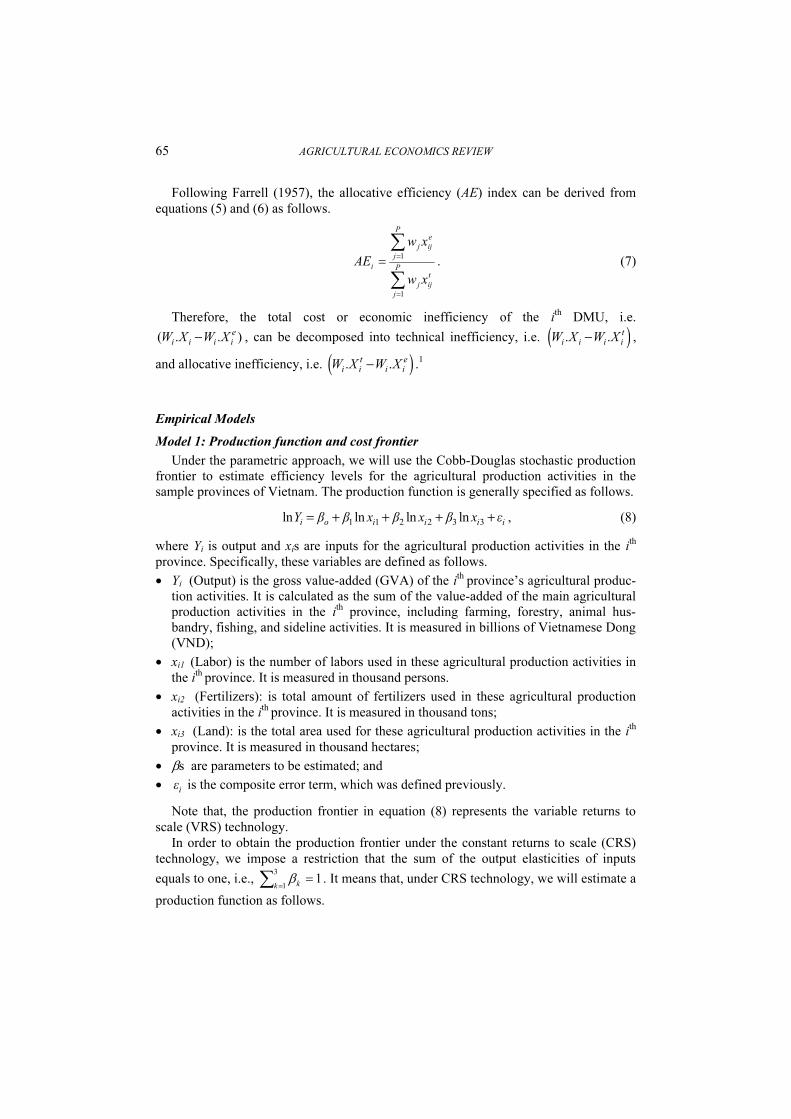
Following Farrell (1957), the allocative efficiency (AE) index can be derived from equations (5) and (6) as follows.

∑∑

=

== P

j

tijj

P

j

eijj

ixw

xwAE

1

1 . (7)

Therefore, the total cost or economic inefficiency of the ith DMU, i.e. ( . . )ei i i iW X W X- , can be decomposed into technical inefficiency, i.e. ( ). .

ti i i iW X W X- ,

and allocative inefficiency, i.e. ( ). .

t ei i i iW X W X- .1

Empirical Models Model 1: Production function and cost frontier

Under the parametric approach, we will use the Cobb-Douglas stochastic production frontier to estimate efficiency levels for the agricultural production activities in the sample provinces of Vietnam. The production function is generally specified as follows. 1 1 2 2 3 3ln ln ln lni o i i i iY β β x β x β x ε= + + + + , (8) where Yi is output and xis are inputs for the agricultural production activities in the ith province. Specifically, these variables are defined as follows. • Yi (Output) is the gross value-added (GVA) of the ith province’s agricultural produc-

tion activities. It is calculated as the sum of the value-added of the main agricultural production activities in the ith province, including farming, forestry, animal hus-bandry, fishing, and sideline activities. It is measured in billions of Vietnamese Dong (VND);

• xi1 (Labor) is the number of labors used in these agricultural production activities in the ith province. It is measured in thousand persons.

• xi2 (Fertilizers): is total amount of fertilizers used in these agricultural production activities in the ith province. It is measured in thousand tons;

• xi3 (Land): is the total area used for these agricultural production activities in the ith province. It is measured in thousand hectares;

• βs are parameters to be estimated; and • iε is the composite error term, which was defined previously.

Note that, the production frontier in equation (8) represents the variable returns to scale (VRS) technology.

In order to obtain the production frontier under the constant returns to scale (CRS) technology, we impose a restriction that the sum of the output elasticities of inputs equals to one, i.e., ∑ =

=3

11k kβ . It means that, under CRS technology, we will estimate a

production function as follows.

2009, Vol 10, +o2 66

3 1 1 3 2 2 3ln( / ) ln( / ) ln( / )i i o i i i i iY x α α x x α x x ε= + + + , (9) where • (Yi/xi3) is per-hectare gross value-added of agriculture production activities in the ith

province during the study period; • (xi1/xi3) is per-hectare number of labors. This variable implies the level of labor in-

tensity in agriculture production activities in the ith province during the study period; and

• (xi2/xi3) is per-hectare tons of fertilizers. This variable shows how much fertilizers were used in agriculture production activities in the ith province during the study pe-riod. The cost function can be obtained from production function in equation (8) by solv-

ing the cost-minimizing problem. The dual cost frontier of the production function in equation (8) is then expressed as

follows. 3 0 1 1 3 2 2 3 3ln( / ) ln( / ) ln( / ) lni i i i i i iC W α α W W α W W α Y= + + + , (10) where Ci is the minimum cost for agricultural production activities in the ith province; and iY is the output of the province i. Model 2: Inefficiency effects model

With regard to the technical inefficiency effect model, the component of technical inefficiency effects in the frontier production function is defined to rely on province-specific factors, including capital-labor ratio (which is approximated by the ratio of number of tractors and number of labors) and geographic location (or economic re-gions). The following is the specification for the model 2:

0 1 1 2 2 4 4 5 5 6 6 7 7 8 8 9( / )it kl tu δ δ Ln tractor labor δ x δ x δ x δ x δ x δ x δ x δ t w= + + + + + + + + + + , (11)

where: • Ln(tractor/labor) is the natural logarithm of number of tractors per labor. • x1 is dummy variable =1 if province is in the region 1,2 and = 0 otherwise. • x2 is dummy variable =1 if province is in the region 2, and = 0 otherwise. • x4 is dummy variable =1 if province is in the region 4, and = 0 otherwise. • x5 is dummy variable =1 if province is in the region 5, and = 0 otherwise. • x6 is dummy variable =1 if province is in the region 6, and = 0 otherwise. • x7 is dummy variable =1 if province is in the region 7, and = 0 otherwise. • x8 is dummy variable =1 if province is in the region 8, and = 0 otherwise. • t is time; and • wt is errors terms which are assumed to be independently and identically distributed

followed by the truncation of the normal distribution with zero mean and unknown variance 2

wσ .

67 AGRICULTURAL ECO+OMICS REVIEW

on-parametric Approach The non-parametric approach in this paper is based on the data envelopment analysis

(DEA) technique (Charnes et al., 1978; and Färe et al., 1985, 1994) in order to estimate technical, scale, allocative, and economic efficiency measures for agricultural produc-tion activities in the sampled provinces.

Suppose that we have 0 provinces (0=60), each producing one output by using k=1, 2, …, P inputs. Let Yi be the output the ith province (i=1,2,…, 0), and ikx be the kth in-put of the ith province (i=1,2,…, 0; k=1,2,…, P). Also, let λj (j=1, 2,…, 0) be a weight.

The CRS input-oriented measure of technical efficiency (TE) for the ith province is calculated as the solution to the following programming problem.

,

minCRSi

CRSiθ λ

θ θ= (12) subject to: j

!

jji YY ∑

=

≤1λ , where i=1, 2, …, 0 (13)

ikCRSijk

&

jj xx θλ ≤∑

=1, where i=1, 2, …, 0; k=1, 2, …, P (14)

0λ≥ , (15) where CRS

iθ is the technical efficiency (TE) measure of the ith province under CRS technology.

If 1CRSiθ = , the ith province’s agriculture production is on the frontier and is techni-

cally efficient under CRS. If 1CRSiθ < , the ith province’s agriculture production is below

the frontier and is technically inefficient under CRS. Under CRS DEA, the technically efficient cost of production of the ith province is given by ( ).

CRSi i iW θ X .

In order to derive a measure of the total or overall economic efficiency (CE) index, we solve the cost–minimizing DEA model (Färe et al., 1985, 1994) as follows.

*

minjx λ

*

1ik

P

kik xw∑

=

, (16)

subject to: j

!

jji YY ∑

=

≤1λ , where i=1, 2, …, 0 (17)

*

1ikjk

#

jj xx ≤∑

=

λ , where i=1, 2, …, 0; k=1, 2, …, P (18)

0≥λ , (19) where *

ix is the cost–minimizing or economically efficient input vector for the ith prov-ince, given its input price vector and output level. The CE index for the ith province is

2009, Vol 10, )o2 68

then computed as follows.

∑∑

=

== P

kikik

ik

P

kik

i

wx

wxCE

1

1

*

, (20)

which is the ratio of the minimum cost to the observed cost. The allocative efficiency (AE) index, derived from equations (12) and (20), is ex-

pressed as follows.

ii CRS

i

CEAEθ

= . (21)

It should be noted that equation (17) also accounts for the input slacks, which are not captured by equation (15). Following Ferrier and Lovell (1990), this procedure attrib-utes any input slacks to allocative inefficiency on the ground that slack reflects an inap-propriate input mix.

The overall technical efficiency under CRS (TECRS) can be decomposed into two components, i.e., “purely” technical efficiency and scale efficiency, by solving a VRS DEA model, which is in turn obtained by imposing the additional constraint ∑ =

= j j1

1λ on equation (15) (Banker et al., 1984). Let VRS

iθ denote the TE index of the ith province under VRS (TEVRS), then the technically efficient costs of production of the ith province under VRS is equal to VRS

i

P

kikik xw θ∑

=1

* . Because the VRS analysis is more flexible and envelops the data in a tighter way

than the CRS analysis, we usually have VRS TE measure ( )VRSθ to be equal or greater than the CRS TE measure ( )CRSθ . This relationship is used to obtain a measure of scale efficiency (SE) of the ith province as follows.

CRSi

i VRSi

θSEθ

= , (22)

where SE = 1 indicates scale efficiency, and SE < 1 indicates scale inefficiency. Scale inefficiency is due to the presence of either increasing or decreasing returns to

scale, which can be determined through a non-increasing returns to scale (NIRS) DEA model by substituting the VRS constraint ∑ =

= j j1

1λ with ∑ =≤

j j11λ . Let IRSθ rep-

resent the technical efficiency measure under NIRS specification. If IRS CRSθ θ= , there are increasing returns to scale, and if CRS #IRSθ θ< there are decreasing returns to scale (Färe et al., 1994). Descriptions of Data and Variables

In this paper, we will use panel data of inputs and output for agricultural production

69 AGRICULTURAL ECO)OMICS REVIEW

activities in sixty provinces of Vietnam in the period 1990-2005. The data were col-lected by the General Statistics Office of Vietnam (GSO) through the years.

Table 1 provides statistical summary for output (gross value-added or GVA) and in-puts (labor, machinery, fertilizers, and land). Table 1. Summary of Inputs and Output

Year Obs. GVA (V-D Million)

Labor (1,000 persons)

Tractor (unit)

Fertilizers (1,000 tons)

Land (1,000 hectares)

1990 60 35,650 17,674 25,155 748 6,989 1991 60 36,248 18,270 35,412 1,452 6,921 1992 60 39,003 21,854 37,278 1,426 7,214 1993 60 40,499 22,647 45,026 1,449 7,257 1994 60 41,479 23,276 87,188 2,253 7,276 1995 60 43,541 23,901 95,527 2,398 7,276 1996 60 45,774 23,978 108,397 3,038 7,589 1997 60 48,272 24,601 113,117 3,180 7,743 1998 60 50,767 24,869 120,605 3,297 7,973 1999 60 53,518 25,082 143,360 3,462 8,601 2000 60 55,395 25,221 162,246 3,553 9,230 2001 60 56,147 25,426 161,492 3,513 9,391 2002 60 57,891 25,876 167,322 3,437 9,250 2003 60 62,384 26,620 179,670 3,719 9,554 2004 60 63,960 26,550 193,504 3,776 9,648 2005 60 65,928 26,714 201,490 3,791 9,715

Source: Authors’ estimates. As mentioned earlier, the output is the sum of the value-added of production from

farming, forestry, animal husbandry, fishing, and sideline activities. All the values of GVA reported in Table 1 are adjusted by the Vietnam’s GDP deflator, in which the year 1994 is the base year. As can be seen, the GVA of the agricultural production has in-creased significantly over the past decade.

The number of labors used in the empirical models excludes labor force working for the rural industries, construction, transportation, commerce, and other miscellaneous occupations. Only labors working for farming, forestry, animal husbandry, fishery, and sideline production activities are included.

Machinery is considered as capital input for the agricultural production activities in this paper, and it is measure by the number of tractors used for farming, forestry, animal husbandry, fishery, and sideline production activities, such as plowing, irrigating, drain-ing, harvesting, farm product processing, transportation, plant protection, and stock breeding.

Fertilizers refer to the sum of pure weight of nitrogen, phosphate, potash, and com-plex fertilizers, while land refers to total cultivated areas at the end of each year.

2009, Vol 10, )o2 70

Empirical Results and Analysis Estimated Results from Parametric Approach

We first conduct some hypotheses tests with the maximum–likelihood estimates of parameters in the Cobb-Douglas stochastic frontier production function, defined in equ-ations (8) and (9), which are obtained for the total sample.

Table 2a presents the test results of various null hypotheses on the sample. The null hypotheses are tested by using likelihood ratio test. The likelihood–ratio test statistic is

[ ]0 12 ( ) ( ) ,λ L H L H= - - where L(H0) and L(H1) are the values of the log-likelihood function under the specifications of the null and alternative hypotheses, H0 and H1, re-spectively. If the null hypothesis is true, then λ has approximately a Chi-square (or mixed Chi-square) distribution with degrees of freedom equal to the number of restric-tions. Table 2a. Statistics for Tests of Hypotheses

Critical Value +ull Hypothesis Log-likelihood Function

Test Statistics (λ) 1% 0.5%

Decision

Under the assumptions of CRS 0 : 0H µ = , η=0 300.502 1 : 0H µ π , η=0 331.251

61.489 6.63 Reject

0 : 0H µ = , η=0 300.502 1 : 0H µ = , 0ηπ 322.45

61.489 6.63 Reject

0 : 0H µ = , η=0 300.502 1 : 0H µ π , 0η = 322.45

62.676 8.273 9.634 Reject

0 : 0H µ γ η= = = -296.68 1257.04 Reject Under the assumptions of VRS

0 : 0H µ = , η=0 353.55 1 : 0H µ π ,η=0 362.352

17.604 Reject

0 : 0H µ = , η=0 353.55 1 : 0H µ = , 0ηπ 365.482

23.864 Reject

0 : 0H µ = , η=0 353.55 1 : 0H µ π , 0ηπ 378.161

49.22 Reject

0 : 0H µ γ η= = = -276.863 1310.048 Reject !ote: The critical value for this test involving γ=0 is obtained from Kodde and Palm (1986). Every null

hypothesis is rejected at the 1 percent significance level. Source: Authors’ estimates

71 AGRICULTURAL ECO!OMICS REVIEW

The first null hypothesis test, i.e. ui is nonnegative half normal distribution with µ=0. The results suggest that the technical efficiency component is following the truncated normal distribution.

The second null hypothesis, i.e. there are no technical inefficiency effects or ( )0 : 0H γ µ η= = = , is rejected at 1% significance level for both cases. If the null hy-pothesis is true, there are no frontier parameters in the regression equation, and the es-timation becomes an ordinary least square estimation. The results suggest that the aver-age production function is an inadequate representation of the Vietnamese agricultural sector, and it will underestimate the actual frontier due to technical inefficiency effects.

To estimate production frontier for the agricultural production in the sampled prov-inces, both cases of Cobb-Douglass production function under the CRS and VRS are employed in this paper.

We use the computer program FRONTIER Version 4.1 (Coelli, 1996a) for our esti-mation. The maximum-likelihood (ML) estimates of the parameters for the stochastic production frontier obtained from the program are presented in Table 2b. Table 2b. Maximum Likelihood Estimates for Parameters Models under the Assump-

tion of Constant Returns to Scale (CRS) Model 1 Model 2

Para-meter coeffi-

cient Standard-

error t-ratio coeffi-cient

standard-error t-ratio

Constant α0 9.3890 0.0749 125.2765 8.9459 0.0271 330.1344 Ln(labor/land) α1 0.2737 0.0251 10.8914 0.7315 0.0252 29.0078 Ln(fertilizer/land) α2 0.1782 0.0157 11.3187 0.1526 0.0195 7.8303 Constant δ0 1.1704 0.0421 27.7921 Ln(tractor/labor) δkl -0.0867 0.0089 -9.7453 x1 δ1 -0.3208 0.0425 -7.5422 x2 δ2 -0.1643 0.0349 -4.7145 x4 δ4 0.0370 0.0346 1.0704 x5 δ5 -0.0777 0.0471 -1.6503 x6 δ6 -0.4448 0.0526 -8.4517 x7 δ7 -0.3398 0.0494 -6.8804 x8 δ8 -0.3879 0.0421 -9.2212 t δ9 0.0071 0.0019 3.7263 Sigma-squared σ2 0.1755 0.0332 5.2819 0.0653 0.0028 23.6183 Gama γ 0.8752 0.0207 42.2103 1.0000 0.0000 190801 µ 0.7839 0.0824 9.5163 η 0.0017 0.0018 0.9711 Log Likelihood 331.8482 0.0000 0.0000 -50.2924 0.0000 0.0000

!ote: 2 2 2u v

σ σ σ= + ; and 2 2/u

γ σ σ= . Source: Authors’ estimates.

2009, Vol 10, !o2 72

As expected, the signs of the slope coefficients of the stochastic production frontier are positive and highly significant. The estimate of the variance parameter, γ , is also positive and significantly different from zero, implying that the inefficiency effects are significant in determining the level and the variability of output of the agricultural pro-duction activities in the sampled provinces.

The estimation of Cobb-Douglass production function under the VRS assumption in Table 2b also shows that the output elasticity of labor (0.2737) is higher than the output elasticities fertilizers (0.1782). Thus, it is obvious that the agricultural production activi-ties in the sampled provinces of Vietnam during the study period were heavily relied on labor.

As mentioned, the variance 2σ helps to know whether the sampled provinces had higher production efficiency during the study period, as it represents the total variance of output. This variance contains a random error term ( 2

vσ ) and a technical inefficiency term ( 2

uσ ). Table 2c indicates that 2σ is small (only 0.2286), meaning that there were insignificant changes in the agricultural outputs of the sampled provinces over the past decade. Table 2c. Maximum Likelihood Estimates for Parameters of Inefficiency Model under

the Assumption of Variable Returns to Scale (VRS) Model 1 Model 2

Variables Parameter coefficient Standard-error t-ratio coefficient standard-

error t-ratio Constant β0 11.4232 0.2350 48.6146 8.7966 0.1148 76.6476 Ln(labor) β1 0.0850 0.0335 2.5352 0.7451 0.0390 19.0901 Ln(fertilizer) β2 0.1772 0.0165 10.7407 0.1523 0.0327 4.6583 Ln(land) β3 0.4044 0.0264 15.3105 0.1425 0.0279 5.1145 Constant δ0 1.2204 0.1529 7.9802 Ln(tractor/labor) δkl -0.0878 0.0101 -8.6637 x1 δ1 -0.3365 0.0534 -6.3016 x2 δ2 -0.1823 0.0434 -4.1995 x4 δ4 0.0310 0.0521 0.5943 x5 δ5 -0.0988 0.0509 -1.9398 x6 δ6 -0.4420 0.0672 -6.5750 x7 δ7 -0.3390 0.0596 -5.6901 x8 δ8 -0.3668 0.0506 -7.2486 t δ9 0.0083 0.0032 2.5759 Sigma-squared σ2 0.2286 0.0154 14.8205 0.0658 0.0040 16.5584 Gama γ 0.9127 0.0070 130.2018 1.0000 0.0855 11.6983 µ 0.9137 0.0578 15.8193 η 0.0079 0.0014 5.5913 Log Likelihood 378.1612 0.0000 0.0000 -48.5002 0.0000 0.0000 !ote:

2 2 2u v

σ σ σ= + ; and 2 2/u

γ σ σ= .

Source: Authors’ estimates.

73 AGRICULTURAL ECO!OMICS REVIEW

In both Table 2b and 2c, the estimates for variables representing regions show a posi-tive and statistically significant coefficient for the Region 4, while negative and statisti-cally significant coefficients for other seven regions. In other words, location had sig-nificant impacts on the efficiency of the studied agricultural production activities. Also, in both Tables 2b and 2c, the coefficients for the variable representing capital-labor ratio, i.e. Ln(tractor/labor), are both negative and statistically significant, meaning that technical inefficiency would have been reduced if agricultural labors had been more technically equipped. Table 2d. Maximum Likelihood Estimates for Parameters for Cost Frontier under the

Assumptions of Constant Returns to Scale (CRS) Variables / Parameters Coefficient Standard-error t-ratio LnA -1.4352 0.4400 -3.2614 Ln(W1/W3) 0.4297 0.0258 16.6502 Ln(W2/W3) 0.0762 0.0192 3.9787 LnY 0.4953 0.0369 13.4086 σ2 0.1733 0.0142 12.2297 γ 0.9219 0.0074 124.2878 µ 0.7995 0.1447 5.5241 η -0.0103 0.0017 -5.9350 Log likelihood 499.8574 0.0000 0.0000 A 0.3187

Source: Authors’ estimates. The dual cost frontier model, derived from the stochastic production function, is pre-

sented in Table 2d. In the form of Cobb-Douglas cost function, we have: 0.43 0.0076 0.494 0.4951 2 3( , ) 0.3187C W Y W W W Y=

Again, significant differences between the coefficients for labor (0.43), land (0.494), and fertilizers (0.0076) show that the costs of the agricultural production activities in the sampled provinces were heavily depended on the costs of labor and land.

Table 3 shows the frequency distribution of the estimated technical efficiency meas-ures for the agricultural production of the sampled provinces under CRS and VRS as-sumptions and cost efficiency estimated from cost function under the assumption of CRS. The estimated mean technical efficiency was 46.88 percent under the CRS as-sumption, and 37.32 percent under VRS assumption. These estimates imply that there were considerable inefficiencies in the agricultural production activities of the sampled provinces. In other words, there would be a substantial room for these provinces to im-prove their agricultural production efficiency.

More than 90 percent of the sampled provinces had technical efficiency at less than 60 percent, while only about 5 percent of these province had technical efficiency of more than 80 percent. The estimated results also show that there was a wide range of technical efficiency of agricultural production between the sampled provinces, as the highest efficiency was about 82.68, while the lowest efficiency was only 13.38 percent.

2009, Vol 10, !o2 74

Table 3. Frequency Distribution of Production Efficiency under CRS, VRS, and Cost Efficiency (CE)

Variable Returns to Scale (TEVRS)

Constant Returns to Scale (TECRS)

Cost Efficiency (CE)

Efficiency Range

Mean Std. Dev. Obs. Mean Std. Dev. Obs. Mean Std. Dev. Obs. [0, 0.2) 0.1761 0.0206 9 0.1866 n.a 1 [0.2, 0.4) 0.2722 0.0598 22 0.2972 0.0573 19 0.3282 0.0463 31 [0.4, 0.6) 0.4812 0.0578 25 0.4910 0.0536 26 0.4852 0.0567 25 [0.6, 0.8) 0.6542 0.0148 3 0.6422 0.0303 12 0.6708 0.07034 3 [0.8, 1) 0.8268 n.a 1 0.9101 0.0409 2 0.9951 n.a 1 All 0.3732 0.1577 60 0.4688 0.1618 60 0.4219 0.1326 60 Mean 0.3732 0.4688 0.4219 Median 0.3808 0.4770 0.3942 Maximum 0.8268 0.9390 0.9951 Minimum 0.1338 0.1866 0.2246 Std. Dev. 0.1577 0.1618 0.1326 Obs. 60 60 60 Source: Authors’ estimates.

Estimated Results from /on-parametric Approach

The DEA models are estimated by using the computer program DEAP Version 2.0 (Coelli, 1996b).

Table 4 presents the technical, allocative, and economic efficiency measures esti-mated from the DEA, as well as their frequency distributions. The estimated mean tech-nical efficiency was 66.3 percent for the CRS DEA model (crste), and 72.6 percent for the VRS DEA model (vrste). Only 21.7 percent of the sampled provinces (or 13 out of 60) were in interval of [80 %, 100%) efficient under the CRS DEA model, while 35.6 percent of the sample (or 22 out of 60) were interval of [80 %, 100%) efficient under VRS DEA model. The scale efficiency varied from 60 percent to 100 percent, with a mean of 90.9 percent.

The estimated allocative efficiency indices under CRS assumptions are presented in Table 5. The mean allocative efficiency (AE) and cost efficiency (CE) indices under the CRS assumptions estimated from the cost-minimizing DEA model were 80.52 percent and 50.92 percent, respectively. Therefore, under DEA models, especially with CRS assumption, it is shown that there were substantial inefficiencies in the agricultural pro-duction activities in the sampled provinces during the past decade.

The distribution of the estimated economic efficiency indices in Table 5 shows that there was a wide range of economic efficiency differences. The minimum economic efficiency level was only 24 percent, while the maximum level was as high as 98.69 percent. About 61.7 percent of the sampled provinces (or 37 out of 60) had economic efficiency level between 20 percent and 60 percent, meaning that there was a large room for these economically inefficient provinces to improve their economic efficiency of the agricultural production activities. The number of provinces with economic efficiency

75 AGRICULTURAL ECO!OMICS REVIEW

ranged from 80 percent to 100 percent was extremely low, only about 5 percent (3 out of 60) under CRS DEA model.

Table 4. Frequency Distribution of Production Efficiency

crste (DEA model)

vrste (DEA model) Scale

Range Mean Std.

Dev. Obs. Range

Mean Std. Dev. Obs

Range Mean Std.

Dev. Obs.

[0.2, 0.4) 0.376 0.007 3 [0.4, 0.6) 0.502 0.037 11 [0.6, 0.7) 0.670 0.032 2 [0.4, 0.6) 0.521 0.064 21 [0.6, 0.8) 0.691 0.060 27 [0.7, 0.8) 0.780 0.018 4 [0.6, 0.8) 0.702 0.056 23 [0.8, 1) 0.870 0.056 20 [0.8, 0.9) 0.855 0.027 16 [0.8, 1) 0.887 0.064 13 [1, 1.2) 1.000 0.000 2 [0.9, 1) 0.957 0.028 38 All 0.663 0.162 60 All 0.726 0.150 60 All 0.909 0.078 60 Mean 0.663 0.726 0.909 Median 0.652 0.731 0.927 Maximum 0.989 1.000 0.995 Minimum 0.370 0.446 0.647 Std. Dev. 0.162 0.149 0.078 Obs. 60 60 60 Source: Authors’ estimates. Table 5. Frequency Distributions of Production Efficiency under CRS and VRS, esti-

mated from the cost-minimizing DEA model AE CE

Range Mean Std. Dev. Obs. Range Mean Std. Dev. Obs. [0.6, 0.7) 0.6615 0.0202 5 [0.2, 0.4) 0.3275 0.0540 13 [0.7, 0.8) 0.7591 0.0279 24 [0.4, 0.6) 0.4968 0.0567 24 [0.8, 0.9) 0.8457 0.0313 25 [0.6, 0.8) 0.6703 0.0446 20 [0.9, 1) 0.9411 0.0310 6 [0.8, 1) 0.9215 0.0648 3 All 0.8052 0.0775 60 All 0.5392 0.1627 60 Mean 0.8052 0.5392 Median 0.8038 0.5427 Maximum 0.9978 0.9869 Minimum 0.6344 0.2400 Std. Dev. 0.0775 0.1627 Obs. 60 60 Source: Authors’ estimates. A Comparison of Parametric and 1on-parametric Estimates

In this paper we applied two approaches to estimate technical, allocative, and eco-

2009, Vol 10, 9o2 76

nomic efficiency measures for the agricultural production activities, in which the para-metric approach is based on SFPF technique, while the non-parametric is based on DEA technique. It might not be expected that efficiency estimates obtained from one tech-nique would be more (or less) than those obtained from the other technique. However, in this paper, we can see that the estimated average efficiency levels based on SFPF model under CRS and VRS (37.32 percent and 46.88 percent, respectively) are much lower than those obtained from DEA model (66.3 percent and 72.6 percent, respec-tively).

The question is why these approaches provided different estimated results under the same assumptions on returns to scale, and the same set of data? To examine this ques-tion, we compute the Spearman rank correlations between efficiency rankings of the sampled provinces. The results are presented in Table 6.

Table 6. Spearman Rank Correlations

Efficiency SFPF DEA Spearman rank correlation (p) Probability TECRS 46.88 66.3 0.8724 0.000 TEVRS 37.32 72.6 0.6472 0.000 CECRS 42.18 53.92 0.3025 0.0178

Source: Authors’ estimates. The results show that, on average, the estimated technical efficiency levels under

CRS and VRS assumptions from SFPF model are significantly smaller than those from DEA model. Therefore, under the same set of data, the assumption on returns to scale is found to be critical in explaining the differences in efficiency measures obtained from these approaches.

However, it is not really surprised to have such different estimates from two ap-proaches, as these estimates are consistent with the expectation that efficiency scores obtained from the non-parametric approach would be higher than those from the para-metric approach. This comment has been indicated in a number of existing studies. For instance, Drake and Weyman-Jones (1996), exploring the UK building firms, produced insignificant rank correlation coefficients between the estimated efficiency levels from both approaches. Ferrier and Lovell (1990) found higher technical efficiency, but lower economic efficiency for the parametric method in comparison with the non-parametric method, and insignificant rank correlations between the estimated efficiencies from two approaches. Using the data for the Guatemalan farmers, Kalaitzandonakes and Dunn (1995) reported a significantly higher level of mean technical efficiency under CRS DEA than under the stochastic frontier.

The differences in the estimated results from two approaches could be mainly attrib-uted to the different characteristics of the data, the choice of input and output variables, measurement and specification errors, as well as estimation procedures.

Concluding Remarks

This paper uses and compares both parametric and non-parametric approaches in es-

77 AGRICULTURAL ECO9OMICS REVIEW

timating technical, allocative, and economic efficiency measures for the agricultural production activities in sixty provinces of Vietnam during 1990-2005. The parametric approach is based on Kopp and Diewert (1982)’s cost decomposition to estimate effi-ciency measures for a Cobb-Douglas stochastic production function and dual cost fron-tier, while the non-parametric approach is based on various input-oriented DEA models.

Under the CRS specification, the average technical, allocative, and economic effi-ciency estimates were 66.3 percent, 80.52 percent, and 53.92 percent, respectively, in parametric approach, and 46.88 percent, 90.35 percent, and 42.18 percent, respectively, in non-parametric approach. Under the VRS specification, technical efficiency esti-mated from parametric approach was 37.32 percent, in non-parametric approach, while it was 72.6 percent. On average, the estimated technical and economic efficiencies were significantly higher in the non-parametric approach than in parametric approach. How-ever, the efficiency rankings of the sampled provinces based on these two approaches are positively and significantly correlated.

By operating at full economic efficiency levels, the sampled provinces would be able to reduce their costs of agricultural production activities about 46 to 76 percent, depend-ing upon the estimation approach and the assumption on returns to scale. In other words, there would be a large room for the studied provinces to improve their agricultural pro-duction efficiency.

The comparison of the estimated results from two approaches shows that they were different, in which DEA provided higher estimates than those from SFPF. The differ-ences could be attributed to various reasons, such as the choice of input and output vari-ables, and measurements and specification errors.

6otes 1 X.Y denoting dot product (or scalar product) for two vectors 1 2( , , ..., )nX x x x= and

1 2( , , ..., )nY y y y= . Thus, i

n

ii yxYX ∑

=

=

1. .

2 In Vietnam, there are eight economic regions: Northeast (Region 1), Northwest (Re-gion 2), Red River Delta (Region 3), North Central Coast (Region 4), South Central Coast (Region 5), Central Highlands (Region 6), Southeast (Region 7), and Mekong River Delta (Region 8).

References Aigner, D. J.; Lovell, C. A. K; Schmidt, P. 1977. Formulation and Estimation of Stochastic

Frontier Production Models, Journal of Econometrics, 6, 21-37. Banker, R. D.; Charnes, A.; Cooper, W. W. 1984. Some Models for Estimating Technical and

Scale Inefficiencies in Data Envelopment Analysis. Management Science 30, No. 9, 1078–1092.

Battese, G.E.; Coelli, T. J. 1992. Frontier Production Functions, Technical Efficiency, and Panel Data: With Application to Paddy Farmers in India. Journal of Productivity Analysis , 3, 153-169.

Charnes, A.; Cooper, W. W; Rhodes, E. 1978. Measuring the Efficiency of Decision Making Units. European Journal of Operational Research 2, 429–444.

2009, Vol 10, 9o2 78

Coelli, T. J. 1996a. A Guide to Frontier Version 4.1: A Computer Program for Stochastic Frontier Production and Cost Function Estimation. Center for Economic Productivity Anal-ysis (CEPA) Working Paper No. 7/96. University of New England, Armidale.

Coelli, T. J. 1996b. A Guide to DEAP Version 2.1: A Data Envelopment Analysis (Computer) Program. Center for Economic Productivity Analysis (CEPA) Working Paper No. 8/96. University of New England, Armidale.

Drake, L. and Weyman-Jones, T.G. 1996. Productive and Allocative Inefficiencies in UK Build-ing Societies: A Comparison of Non-Parametric and Stochastic Frontier Techniques. The Manchester School, 64, 22-37.

Färe, R.; Grosskopf, S; Lovell, C. A. K. 1985. The Measurement of Efficiency of Production. Kluwer-Nijhoff Publication, Boston.

Färe, R.; Grosskopf, S; Lovell, C. A. K. 1994. Production Frontiers. Cambridge University Press, New York.

Farrell, M. J. 1957. The Measurement of Productive Efficiency. Journal of Statistical Society, Series A (General) 120, no. 3, 253–290.

Ferrier, G. D.; Lovell, C. A. K. 1990. Measuring Cost Efficiency in Banking: Econometric and Linear Programming Evidence. Journal of Econometrics, Vol. 46, Issues 1-2, 229–245.

Kalaitzandonakes, N. G.; Dunn, E. G. 1995. Technical Efficiency, Managerial Ability, and Farmer Education in Guatemalan Corn Production: A Latent Variable Analysis. Agricul-tural Resource Economic Review, 24, 36-46.

Kodde, D. A.; Palm, F. C. 1986. Wald Criteria for Jointly Testing Equality and Inequality Re-strictions, Econometrica, 54(5), 1243-48.

Kopp, R. J.; Diewert, W. E. 1982. The Decomposition of Frontier Cost Function Deviations into Measures of Technical and Allocative Efficiency. Journal of Econometrics, 19, 319-331.

Meeusen, W.; Van de Broeck, J. 1977. Efficiency Estimation from Cobb-Douglas Production Function with Composed Error. International Economic Review, 18, 435-44.

Ministry of Foreign Affairs of Vietnam (MOFA). 2007. Nong nghiep Vietnam nhung nam gan day (Vietnam’s Agriculture in Recent Years). Retrieved on February 3, 2007 from http://www.mofa.gov.vn/vi/tt_baochi/nr041126171753/ns050302091607.

Nguyen, K. M.; and Vu, Q. D. 2004. Non-parametric Analysis of Technical, Pure Technical, and Scale Efficiencies for the Aquaculture-processing Firms in Vietnam. In Proceedings of International Conference on Vietnam–Thailand Economic and Development Cooperation. National Economics University, Hanoi.

Nguyen K. M. 2005. A Comparative Study on Production Efficiency in Manufacturing Indus-tries of Hanoi and Ho Chi Minh Cities. Vietnam Development Forum (VDF) Discussion Paper, No.3(E). Vietnam Development Forum, Hanoi.

Nguyen, K. M.; and Giang, T. L. (eds.). 2007. Technical Efficiency and Productivity Growth in Vietnam: Parametric and Gon-parametric Analyses. The Publishing House of Social La-bour, Hanoi.

Sharma, K. R., P. Leung; and H. M. Zaleski. 1999. Technical, Allocative, and Economic Effi-ciencies in Swine Production in Hawaii: A Comparison of Parametric and Non-parametric Approaches. Agricultural Economics 20(1), 23-35.

Shephard, R. W. 1970. The Theory of Cost and Production Functions. Princeton University Press, New Jersey.