Technical Efficiency in the Agricultural Sector– Evidence from … · 2017-07-16 · 100...
24
100 AGRICULTURAL ECOOMICS REVIEW Technical Efficiency in the Agricultural Sector– Evidence from a Conditional Quantile - Based Approach Sofia Kourtesi 1 , Kristof De Witte 2 , Apostolos Polymeros 3 1 Department of Economics, Aristotle University of Thessaloniki, Greece 2 Top Institute for Evidence Based Education Research, Maastricht University, the etherlands; and Faculty of Business and Economics, Katholieke Universiteit Leuven (KULeuven), Belgium 3 Department of Statistics, Athens University of Economics and Business, Greece; and EU Farm Accounting Data etwork, Ministry of Rural Development and Food, Greece Abstract The tightening farm budget constraints due to the reduction of the agricultural public financing and the negative gap between the agricultural input and output prices should force farms to work as efficient as possible. This paper applies a fully nonparametric approach to estimate potential efficiency gains in the agricultural sector while account- ing for heterogeneity among farms. Using the ‘conditional α -quantile robust partial frontier technique’ we investigate the efficiency of agricultural enterprises specialized in cereals production. The data originate from the EU Farm Accounting Data etwork. The results indicate a considerable variability in terms of technical efficiency among farms. We find evidence that the owned to total land, the family to total labor, the irri- gation system, the region at which the farm is located and the year of observation have a statistically significant impact on productivity. Keywords: Agriculture, Efficiency, Conditional α -quantile robust partial frontier JEL Classification: D23, Q12 1. Introduction The tightening budget constraints, due to the reduction in agricultural subsidies and the negative gap between the agricultural input and output prices, force farms to work as efficient as possible. The decrease in agricultural subsidies arises from the changes in the European Union’s (EU’s) Common Agricultural Policy (CAP). While the CAP budget amounted to 0.46% of the EU gross national income (GNI) in 2000, it is - 0.34% of the EU GNI in 2011. Another reduction in farm income originates from a significant deviation between the agricultural input prices and the agricultural output prices. While the agricultural input prices are rising over time, the respective output prices are dimin- ishing. One such case is Greece in which the agricultural input price index increased from 100 in 2005 to 112.2 in 2011, whereas the agricultural output price index de- creased from 100 in 2005 to 82.9 in 2011. Obtaining insights in the relative efficiency could allow managers and policy makers to offset the consequences of decreasing budg- ets.
Transcript of Technical Efficiency in the Agricultural Sector– Evidence from … · 2017-07-16 · 100...
100 AGRICULTURAL ECO�OMICS REVIEW
Technical Efficiency in the Agricultural Sector–
Evidence from a Conditional Quantile - Based Approach
Sofia Kourtesi1, Kristof De Witte
2, Apostolos Polymeros
3
1 Department of Economics, Aristotle University of Thessaloniki, Greece
2 Top Institute for Evidence Based Education Research, Maastricht University, the �etherlands;
and Faculty of Business and Economics, Katholieke Universiteit Leuven (KULeuven), Belgium
3 Department of Statistics, Athens University of Economics and Business, Greece;
and EU Farm Accounting Data �etwork, Ministry of Rural Development
and Food, Greece
Abstract
The tightening farm budget constraints due to the reduction of the agricultural public
financing and the negative gap between the agricultural input and output prices should
force farms to work as efficient as possible. This paper applies a fully nonparametric
approach to estimate potential efficiency gains in the agricultural sector while account-
ing for heterogeneity among farms. Using the ‘conditional α -quantile robust partial
frontier technique’ we investigate the efficiency of agricultural enterprises specialized
in cereals production. The data originate from the EU Farm Accounting Data �etwork.
The results indicate a considerable variability in terms of technical efficiency among
farms. We find evidence that the owned to total land, the family to total labor, the irri-
gation system, the region at which the farm is located and the year of observation have
a statistically significant impact on productivity.
Keywords: Agriculture, Efficiency, Conditional α -quantile robust partial frontier
JEL Classification: D23, Q12
1. Introduction
The tightening budget constraints, due to the reduction in agricultural subsidies and
the negative gap between the agricultural input and output prices, force farms to work as
efficient as possible. The decrease in agricultural subsidies arises from the changes in
the European Union’s (EU’s) Common Agricultural Policy (CAP). While the CAP
budget amounted to 0.46% of the EU gross national income (GNI) in 2000, it is - 0.34%
of the EU GNI in 2011. Another reduction in farm income originates from a significant
deviation between the agricultural input prices and the agricultural output prices. While
the agricultural input prices are rising over time, the respective output prices are dimin-
ishing. One such case is Greece in which the agricultural input price index increased
from 100 in 2005 to 112.2 in 2011, whereas the agricultural output price index de-
creased from 100 in 2005 to 82.9 in 2011. Obtaining insights in the relative efficiency
could allow managers and policy makers to offset the consequences of decreasing budg-
ets.
2016, Vol 17, �o 2 101
Over the past 40 years, the efficiency literature has largely evolved around two alter-
native methodological approaches to measure (in)efficiency. While both approaches
consider relative efficiency, they differ in the assumptions they impose on the observed
data. The parametric approach augments the classical regression model by a non-
positive error term capturing technical inefficiency in production (e.g. Battese and
Coelli, 1988; Stevenson, 1980; Aigner et al., 1977). Similar parametric methods require
restrictions on the shape of the production frontier. Therefore, they lack robustness
when the functional form of the frontier and/or the error structure are not correctly
specified, which is often the case in applications (Yatchew, 1998). In farming, for ex-
ample, there is no evidence on the correct specification of the production frontier, which
is likely to result in biased parametric estimations.
The non-parametric approach involves the nonparametric envelopment of a given
sample of observations by a piece-wise linear hull. Non-parametric models such as the
Data Envelopment Analysis (DEA; Charnes et al., 1978) and the Free Disposal Hull
(FDH; Deprins et al., 1984) dispense with the need to specify functional forms and error
structures and appear to be quite appealing for efficiency analysis. The original contri-
butions rely, however, on a deterministic assumption: all observations belong to the
production set with probability equal to 1. Consequently, they are sensitive to noise,
outliers and/or measurement errors. This might impose endogeneity issues if the amount
of output is subject to random shocks. In farming, for example, the level of realized
output can be different from the expected output because of weather conditions and pest
attacks. The corresponding noise results in biased estimates where ‘efficient’ observa-
tions are basically productions without negative shocks.
Despite the discussed risks of applying the parametric and non-parametric ap-
proaches to the agricultural sector, there are numerous applications in the academic lit-
erature. An overview is provided by Mendes et al. (2012) and Bravo-Ureta and Pinheiro
(1993) for parametric applications to the agricultural sector, and by Tavarez (2009) for
non-parametric applications. Examples include Giannakas et al. (2001), Tzouvelekas et
al. (2002), Madau (2007), Hassine (2007) and Barnes (2008). These studies implement
a two-stage procedure in order to investigate the causes of technical inefficiency. In a
first stage, the relative efficiencies are estimated using the Stochastic Frontier Analysis,
while in a second stage the correlation of farm-specific factors on efficiency is esti-
mated. For the non-parametric set-up, recent research with applications to the agricul-
tural sector include Lansink et al. (2002), Thiele and Brodersen (1999), Brummer
(2001), Kuosmanen et al. (2006), Cherchye and Van Puyenbroeck (2007), André
(2009), Latrufee et al. (2008; 2012) and Galanopoulos et al. (2011).
This paper implements a more recent approach to measure relative efficiency in the
agricultural sector. The approach accommodates the drawbacks of the parametric and
non-parametric approach. It follows a recent research avenue comprising nonparametric
efficiency estimators that are robust to atypical observations. The order-m estimator in-
troduced by Cazals et al. (2002) and the a-quantile estimator introduced by Aragon et al.
(2005) rely on partial frontiers which do not envelop all data points. As such, the partial
frontiers provide less extreme surfaces to benchmark the individual production units
and, thus, they are less vulnerable to extreme observations compared to the full fron-
tier1.
1 Since the a-quantile estimator is a deterministic estimator it does not allow for an error term or meas-
102 AGRICULTURAL ECO�OMICS REVIEW
The robust efficiency estimators have the same asymptotic properties as the FDH and
the DEA estimators but they attain better convergence rates (Daraio and Simar, 2007;
Aragon et al., 2005; Cazals et al., 2002).
It has long been recognized that efficiency estimates which do not account for the
operational environment of individual production units have only a limited value.
Therefore, if the units in a given sample are influenced by environmental/exogenous
factors the efficiency analysis should control for this heterogeneity (e.g. Daraio and Si-
mar, 2005; De Witte and Kortelainen, 2013). Parametric approaches control for the in-
fluence of background variables in a similar way as standard econometric techniques
account for heterogeneity. As a disadvantage, again, it requires strong parametric as-
sumptions. The nonparametric approaches typically capture the influence of background
variables in a two-stage approach where the relative efficiency estimates are correlated
to control variables. While there is a large debate on the appropriate procedure and use-
fulness of the approach (e.g., Simar and Wilson, 2007; Banker and Natarajan, 2008), all
current suggestions still rely on model specifications for the second stage (in particular,
bootstrapping in the suggestion of Simar and Wilson, 2007; parametric specification in
the suggestion of Banker and Natarajan, 2008). On the contrary, the partial frontiers are
based on a probabilistic formulation of the production process. This paper adopts a pro-
cedure to incorporate the operating environment in a very natural way in the partial
frontiers (that is, by conditioning on the exogenous environment). The so-called ‘condi-
tional efficiency approach’ generalizes previous models and allows a researcher to in-
vestigate the impact of environmental variables on the distribution of efficiencies.
Moreover, it dispenses with the separability condition and it does not require any a pri-
ori specification regarding the impact of exogenous factors.2
The robust nonparametric efficiency estimators have been applied to banking, mutual
funds, post offices, and education (e.g. De Witte and Kortelainen, 2013; Halkos and
Tzeremes, 2011; Wheelock and Wilson, 2008 and 2009; Daouia and Simar, 2007; Da-
raio and Simar, 2007; Aragon et al., 2005). To our best knowledge, however, analogous
implementations to the agricultural sector are less than a handful. This is disconcerting
since, as argued before, the approaches relying on partial frontiers are very suitable for
measuring efficiency in the presence of random shocks and unknown production fron-
tiers.
In summary, this paper contributes to the literature in three aspects. First, as dis-
cussed before, it applies the nonparametric robust α -quantile procedure to the condi-
tional efficiency framework.3 Second, it applies nonparametric efficiency approaches to
the cereal sector utilizing panel data. To our best knowledge, this is the first paper to do
urement errors in the data generating process. However, since a partial frontier model is robust to out-
liers and extreme points it is suitable for efficiency estimation when the output is subject to random
shocks. 2 The separability condition holds when the environmental variables affect only the distribution of the
efficiencies and not the range of achievable input-output combinations (shape of the production set). In
cases where the separability condition does not hold the two-stage approaches are inappropriate and ef-
ficiency estimation conditionally on environmental variables can be used (Daraio et al, 2010). 3 The a-quantile estimator is continuous and, thus, capable of covering the interior of the attainable set
entirely. It has, therefore, from an economic standpoint an advantage over the discrete order-m estima-
tor (that is, it gives a clearer indication of technical efficiency) (Aragon et al., 2005).
2016, Vol 17, �o 2 103
so. In particular, we use a sample of cereal farms in Greece. The data originate from the
EU Farm Accounting Data Network (FADN) for the years 2008-2011. Derived from
national survey data, FADN is an extremely rich and harmonized source of microeco-
nomic data. This makes it suitable for efficiency analysis (see also Lansink et al., 2002;
Scardera and Zanoli, 2002). Third, using insights from nonparametric econometrics, we
reveal which control variables influence efficiency. This yields insights for policy mak-
ers and farm’s managers.
The remainder of this paper unfolds as follows. Section 2 presents the suggested ana-
lytical framework of the conditional α -quantile efficiency measures. Section 3 dis-
cusses the data and the empirical results. Section 4 offers conclusions and suggestions
for future research.
2. Analytical Framework
2.1 The Unconditional α -Quantile Estimator
To estimate relative efficiency, we relate the resources (inputs) of observations to the
produced outcomes (outputs) of observations. Let pRX
+∈ be the vector of inputs and
qRY
+∈ be the vector of outputs from a given production process. Let Ψ be the produc-
tion possibility set (that means, the set of all feasible input-output combinations). Ψ sat-
isfies the assumption of free disposability (e.g. Deprins et al, 1984). As noted by Cazals
et al. (2002), the production process can be described by the joint probability measure
of ),( YX on qpxRR
++. This joint probability measure is completely characterized by the
knowledge of the probability function:
(1) ( , ) ( , )XY
H x y prob Y y X x= ≥ £
Equation (1) gives the probability that an observation that operates at level ),( yx is
dominated. The support of XY
H is the production set .Ψ Relation (1) can be expressed
as:
(2) ( , ) ( ) ( ) ( ) ( )XY XY X
H x y prob Y y X x prob X x S y x F x= ≥ £ £ =
where )( xySXY
denotes the (non-standard) conditional survival function of Y and
)(xFX
for the distribution function of .X The traditional nonparametric efficiency estimators are deterministic in nature since
they assume that 1),( =Ψ∈yxprob (meaning that all observations belong to the pro-
duction set). They are therefore sensitive to outliers: observations that heavily influence
estimates of the upper boundary of the support of )(| xySXY
.
To reduce the influence of outliers, various approaches have been suggested. Daraio
and Simar (2005) proposed the ‘robust order-m method’. This approach draws repeat-
edly and with replacement m observations with lower inputs (in the output-oriented
case) or with more outputs (in the input-oriented case) from the sample, and estimates
efficiency relative to these smaller subsamples. The robust order-m method mitigates
the influence of outliers as an outlying observation does not constitute the reference set
in every subsample.
104 AGRICULTURAL ECO�OMICS REVIEW
The paper at hand focuses on an alternative approach suggested by Aragon et al.
(2005). They proposed the ‘α -quantile efficiency estimator’. Daouia and Simar (2007)
extended the method to allow for production processes involving multiple inputs and
outputs. Specifically, for all x such that 0)( >xFx
and for ]1,0(∈α , Daouia and Simar
(2007) define the α -quantile output efficiency score for the unit operating at level
( , )x y as:
(3) { }( , ) sup ( ) 1α Y Xλ x y λ S λy x a= > -
When 1),( =yxa
λ , the unit belongs to the α -quantile frontier meaning that only
%100)1( α− of the units using inputs less than (or equal to) x dominate it. When
1)(),( <>yxa
λ a proportional increase (decrease) in all outputs is necessary to bring the
unit ),( yx on the α -quantile frontier. On the basis of (3), the α -quantile frontier is the
pxq vector )),(,( yyxxa
λ where .),( Ψ∈yx In the special case with 1=q ,
)(),()( xyyxxya
E φλ ==
stands for the α -quantile production function.
The traditional FDH estimator is a special case of the α -quantile estimator. In par-
ticular, if 1=α the α -quantile efficiency score reduces to that obtained from the FDH
estimator. It is clear that the FDH estimator envelops all data points such that it is sensi-
tive to outlying observations. With ,1<α the α -quantile frontier is a partial estimator.
Because of its continuous ‘trimming’ nature, the α -quantile efficiency estimator does
not envelope all data points; it allows for ‘super-efficient’ units (meaning those with
1<a
λ ) to be located outside the estimated frontier and, thus, it avoids the problems of
deterministic estimators such as in FDH (which is also the case in the order-m model).
Technical details on the empirical implementation of (3) with n production units in a
sample are presented in the Appendix (part A).
As a major advantage on the order-m approach, the α -quantile approach can better
handle random variation in the outputs, since the extremeα -quantile efficiencies are
more robust than extreme order-m measures (Daouia and Simar, 2007). The latter is
convenient in the agricultural sector, where outputs yearly differ because of unmeasured
variation (due to, e.g., weather conditions). As a disadvantage, the α -quantile frontier
requires a selection of the size of α . We follow Daraio and Simar (2006 and 2007) and
choose an appropriate level for α such that to achieve an adequate level of robustness.4
2.2 The Conditional α -Quantile Estimator
In previous section, we presented the unconditional α -quantile estimator. This esti-
mator does not account for heterogeneity in the sample. In most applications, however,
ignoring the heterogeneity among observations results in biased estimates. This section
outlines the conditional α -quantile estimator, which does capture in a nonparametric
way the differences among observations.
Let r
RZ∈ denote a vector of environmental (or control) variables which may (or
may not) influence the relative performance of observations. To account for the opera-
4 The level of robustness refers to the percentage of the sample points to be left outside of the partial
frontier (that means, the percentage of ‘‘super-efficient’’ units in the sample).
2016, Vol 17, �o 2 105
tional environment in efficiency estimation with partial frontiers, Cazals et al. (2002)
considered the data generating process of the random variable ),,( ZYX and focused on
the conditional distribution of ),( YX for a given value of Z :
(4) | |,( , | ) ( , ) ( , ) ( / )
XY Z X ZY X ZH x y z prob Y y X x Z z S y x z F x z= ≥ £ = =
giving the probability that the unit ),,( zyx will be dominated by other units facing ex-
actly the same operational environment (that means, having zZ = ). The support of
ZXYH is denoted by Z
Ψ (a set possibly different from the production set ).Ψ Daouia
and Simar (2007) defined the conditional α -quantile efficiency estimator as:
(5) { },
( , ) sup ( , ) 1α Y X Zλ x y z λ S λy x z a= > -
),( zyxa
λ has an interpretation analogous to that of ),( yxa
λ ; that is,
%100)),(1( zyxa
λ− stands for the radial feasible change in all outputs a unit operating
at ).,( zyx should perform to reach the efficient boundary of the set z
Ψ . Technical de-
tails on the empirical implementation of (5), including an operationalization of zZ = by a kernel approach, are presented in the Appendix (part B).
2.3 The influence of Environmental Factors
Finally, it is interesting to examine the influence of environmental/exogenous factors
on the relative efficiency of the observations. Environmental factors can both have a
favorable (e.g., soil fertility) or unfavorable (e.g., soil roughness) influence on the effi-
ciency of the observations.
One can nonparametrically examine the correlation between the environmental vari-
ables and the efficiency estimates by using the ratio of the conditional to the uncondi-
tional a-quantile efficiency scores (that means the ratio of the radial distances from the
conditional and the unconditional frontiers, respectively). Specifically, Daraio and Si-
mar (2005, 2007) propose the estimation of the following nonparametric regression
model:
(6) ,
( )n i i i
g z eϕ = +
where
(7) , ,
,
, ,
( , )( , ) , 1, 2,..., ,
( , )
a n ii i i
n i i i i
a n ii i
x y zx y z i n
x y
λϕ
λ
∧
∧= =
g denotes a conditional mean function, and ie stands for an error term (with
).0)( =iizeE The nonparametric regression line indicates whether the environmental
variable has a favorable or unfavorable influence on the efficiency. In the output-
oriented analysis, and for a univariate and continuous Z , a horizontal smoothed regres-
sion curve implies that the environmental factor has no influence on efficiency; an in-
creasing (decreasing) regression curve implies that efficiency rises (falls) with the
amount of Z . Environmental variables with a favorable impact behave as a substitute
106 AGRICULTURAL ECO�OMICS REVIEW
input which augments the productivity of the inputs X . In the opposite case, the pres-
ence of Z reduces productivity by entailing more of the inputs X per unit of output. It
should be noted that the impact is not necessarily monotonic for all values of Z . An
increasing part of the regression may be followed by a decreasing one (and the oppo-
site).
De Witte and Kortelainen (2013) extended the ideas of Daraio and Simar (2005 and
2007) to general Z vectors involving mixed continuous and discrete (both ordered and
unordered) environmental variables. Moreover, they developed appropriate tools of sta-
tistical inference. With multiple Z factors, the visualization of individual impacts can
be achieved through the so-called partial smooth regression plots where only one such
factor at a time is allowed to change and the rest are kept at fixed values (for instance,
the rest of the continuous factors are set at the first, the second or the third quartile,
while the discrete factors are evaluated once at each category).
The statistical inference relies on the Local Linear model which allows the estima-
tion of both the continuous smooth function in (6) as well as the gradient vector associ-
ated with the individual environmental factors (Racine et. al., 2006).5 The Local Linear
method involves the following minimization problem:
(8) 2{ , }
1
min ( ( )) ( , ),
nc c
γ δ i i h i
i
φ γ δ z z K z z
Ÿ
=
- - -Â
where ),,(u
i
o
i
c
iizzzz = includes the values of the continuous and the discrete (ordered
and unordered) environmental variables, γ and δ are local coefficients, and h
K is the
generalized product kernel function with appropriate bandwidth; the gradient vector of
interest is )(c
zδ . Let ZZs∈
be the s the component of vector Z and
OZ be the vector
of all other environmental variables. Then, the null hypothesis (no influence) is:
(9) ( , )
( , ) ( ) 0 ( ) 0 almost everywheres O
s O O s
s
E φ Z ZE φ Z Z E φ Z δ Z
Z
∂= fi = fi =
∂
and the alternative is 0)( ≠s
Zδ (De Witte and Kortelainen, 2013). Details on the esti-
mation of the gradient )(c
zδ and the associated with it vector of p - values are pre-
sented in the Appendix (Part C). The p - values together with the partial smooth re-
gression plots allows a researcher to characterize the sign of the impact of each individ-
ual environmental factor on efficiency as well as its statistical significance.
3. Technical Efficiency of Cereal Farms
3.1 Selection of input, output and environmental variables
Using the outlined conditional efficiency framework, we examine the relative effi-
ciency of agricultural enterprises specialized in cereals production in Greece. Greece
makes an interesting case study as efficiency improvements are necessary to offset the
5 Compared to alternative nonparametric regression estimators (e.g. the Nadaraya-Watson one), the Lo-
cal Linear Estimator is less sensitive to boundary effects.
2016, Vol 17, �o 2 107
significant deviation between the agricultural input-output prices and the decrease of
EU agricultural subsidies. The choice of enterprises specialized in cereals production is
based on the fact that cereals are the most basic nutrition product. In Greece and in the
European Union cereals are cultivated in about the 1/4th and 1/3th of the total cultivated
land respectively (European Commission, 2012).
The empirical analysis relies on a panel data set coming from the Farm Accounting
Data Network (FADN) of the EU. This dataset is a main tool for the Common Agricul-
tural Policy simulations and scenarios implementations. The FADN extracts a represen-
tative sample of farms from the population. In particular, the total population of farms is
first stratified according to their economic size and the type of farming. Stratification is
a classical statistical technique used to increase sample efficiency that is to minimize the
number of farms required to represent the farms in the field of observations. Next,
FADN randomly selects farms within each stratification cluster. The procedure fol-
lowed by each member-state produces weighted samples. The sampling is repeated
yearly. For this paper we used the most recently panel finalized data set which refers to
the accounting years 2008-2011. The FADN, for this time period, provides information
from 632 specialized cereal farms located in all regions of Greece.6
In the conditional α -quantile estimations, we need to specify input and output vari-
ables. Following previous literature (e.g. Giannakas et al., 2001), we used the following
inputs (X): (a) total labor (comprising all family and non-family labor and measured in
working hours); (b) total land (measured in 100m2); (c) fertilizers and pesticides (meas-
ures in Euros); and (d) other costs (including electric power, fuel, seeds, depreciation,
interest and miscellaneous expenses, measured in Euros)7. The selection of the inputs
follows a standard economic theory in which both labour, capital (i.e. land) and re-
sources are used to produce the outputs. Farm output )(Y is the total revenue from crop
production (measured in Euros)8. Our selection of inputs and outputs is in line with pre-
vious literature. In particular, Madau (2007), Giannakas et al. (2001), Tzouvelekas et al.
(2002), Latruffe et al. (2008; 2012), Barnes and Cesar, (2011), Dhehibi et al. (2012)
used similar inputs. Alternative inputs and outputs are used by Amor and Goaied
(2010), Hassine (2007) and Barnes (2008). The latter authors used as inputs irrigated
water, animal traction, rent and other land charges instead of land area, or seed ex-
penses. Alternative outputs used in previous literature include production’s quantity
instead of value.
Summary statistics are provided in Table 1. The average revenue of a specialized
cereal farm is 16,582 euros. The minimum and maximum values are 979 and 70,021
respectively. As we can see in Figure 1, the sample includes very small as well as very
6 FADN considers a farm as a ‘cereal farm’ if it obtains more than 2/3 of its revenues from the produc-
tion of cereals. 7 All the nominal variables were deflated using price indices (base year 2005) from the Hellenic Statisti-
cal Authority. 8 As noted Banker et al. (2007), the use of aggregate revenue or aggregate cost data may result in techni-
cal efficiency estimates reflecting a mix of technical and allocative efficiency. In this paper, we deal
with a single output such that the allocative efficiency from the production side is not an issue. Fertil-
izers, pesticides, as well as “other “ inputs are expressed in monetary units to facilitate aggregation.
This is a very common practice in empirical analysis of technical efficiency (e.g. Latruffe et al., 2008;
Larsen, 2010).
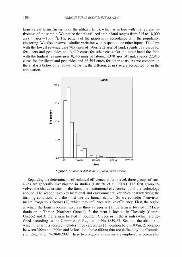
108 AGRICULTURAL ECO�OMICS REVIEW
large cereal farms (in terms of the utilized land), which is in line with the representa-
tiveness of the sample. We notice that the utilized arable land ranges from 215 to 18,000
ares (1 ares = 100 m2). The pattern of the graph is in accordance with the population
clustering. We also observe a similar variation with respect to the other inputs. The farm
with the lowest revenue uses 905 units of labor, 252 ares of land, spends 737 euros for
fertilizers and pesticides and 3,419 euros for other costs. On the other hand the farm
with the highest revenue uses 8,340 units of labour, 5,370 ares of land, spends 22,950
euros for fertilizers and pesticides and 66,595 euros for other costs. As we compare in
the analysis below only look-alike farms, the differences in size are accounted for in the
application.
Figure 1. Frequency distribution of land under cereals.
Regarding the determinants of technical efficiency at farm level, three groups of vari-
ables are generally investigated in studies (Latruffe et al., 2004). The first group in-
volves the characteristics of the farm, the institutional environment and the technology
applied. The second involves locational and environmental variables characterizing the
farming conditions and the third one the human capital. So we consider 7 environ-
mental/exogenous factors )(Z which may influence relative efficiency. First, the region
at which the farm is located involves three categories (1: the farm is located in Mace-
donia or in Thrace (Northern Greece), 2: the farm is located in Thessaly (Central
Greece) and 3: the farm is located in Southern Greece or in the islands) which are de-
fined according to the Commission Regulation No 1859/82. Second, the altitude at
which the farm is located includes three categories (1: location below 300m, 2: location
between 300m and 600m and 3: location above 600m) that are defined by the Commis-
sion Regulation No 868/2008. These two regional dummies are employed as proxies for
2016, Vol 17, �o 2 109
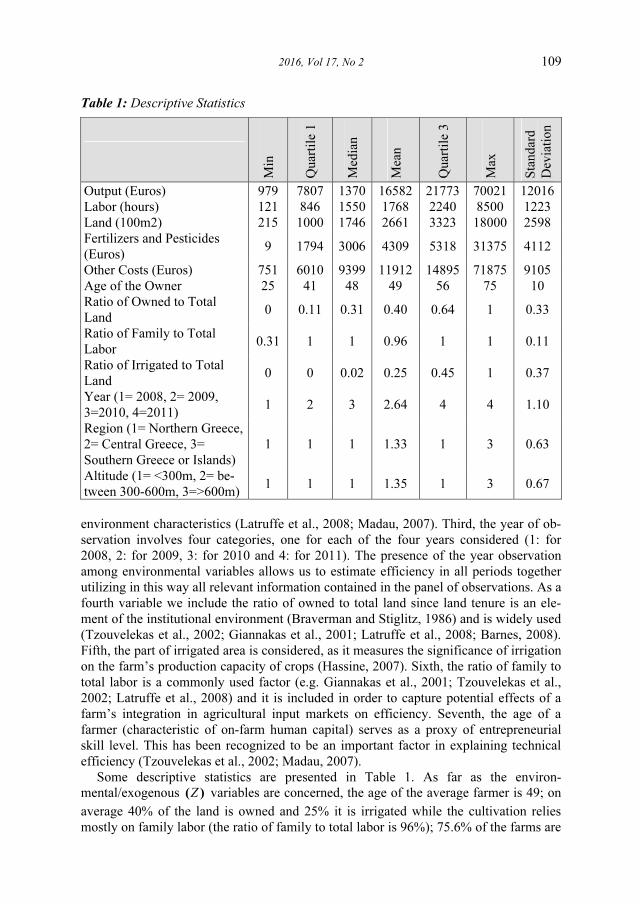
Table 1: Descriptive Statistics
Min
Quar
tile
1
Med
ian
Mea
n
Quar
tile
3
Max
Sta
ndar
d
Dev
iati
on
Output (Euros) 979 7807 1370 16582 21773 70021 12016
Labor (hours) 121 846 1550 1768 2240 8500 1223
Land (100m2) 215 1000 1746 2661 3323 18000 2598
Fertilizers and Pesticides
(Euros) 9 1794 3006 4309 5318 31375 4112
Other Costs (Euros) 751 6010 9399 11912 14895 71875 9105
Age of the Owner 25 41 48 49 56 75 10
Ratio of Owned to Total
Land 0 0.11 0.31 0.40 0.64 1 0.33
Ratio of Family to Total
Labor 0.31 1 1 0.96 1 1 0.11
Ratio of Irrigated to Total
Land 0 0 0.02 0.25 0.45 1 0.37
Year (1= 2008, 2= 2009,
3=2010, 4=2011) 1 2 3 2.64 4 4 1.10
Region (1= Northern Greece,
2= Central Greece, 3=
Southern Greece or Islands)
1 1 1 1.33 1 3 0.63
Altitude (1= <300m, 2= be-
tween 300-600m, 3=>600m) 1 1 1 1.35 1 3 0.67
environment characteristics (Latruffe et al., 2008; Madau, 2007). Third, the year of ob-
servation involves four categories, one for each of the four years considered (1: for
2008, 2: for 2009, 3: for 2010 and 4: for 2011). The presence of the year observation
among environmental variables allows us to estimate efficiency in all periods together
utilizing in this way all relevant information contained in the panel of observations. As a
fourth variable we include the ratio of owned to total land since land tenure is an ele-
ment of the institutional environment (Braverman and Stiglitz, 1986) and is widely used
(Tzouvelekas et al., 2002; Giannakas et al., 2001; Latruffe et al., 2008; Barnes, 2008).
Fifth, the part of irrigated area is considered, as it measures the significance of irrigation
on the farm’s production capacity of crops (Hassine, 2007). Sixth, the ratio of family to
total labor is a commonly used factor (e.g. Giannakas et al., 2001; Tzouvelekas et al.,
2002; Latruffe et al., 2008) and it is included in order to capture potential effects of a
farm’s integration in agricultural input markets on efficiency. Seventh, the age of a
farmer (characteristic of on-farm human capital) serves as a proxy of entrepreneurial
skill level. This has been recognized to be an important factor in explaining technical
efficiency (Tzouvelekas et al., 2002; Madau, 2007).
Some descriptive statistics are presented in Table 1. As far as the environ-
mental/exogenous )(Z variables are concerned, the age of the average farmer is 49; on
average 40% of the land is owned and 25% it is irrigated while the cultivation relies
mostly on family labor (the ratio of family to total labor is 96%); 75.6% of the farms are
110 AGRICULTURAL ECO�OMICS REVIEW
located in Northern Greece and 15.7 % in Central Greece; 75.5% of the farms are lo-
cated below 300m and 13.8% are located between 300m and 600m. As far as the year
variable is considered, 19.5%, 26.6%, 24.1%, and 29.9% of the total observations come
from 2008, 2009, 2010 and 2011 respectively.
The α -quantile efficiency scores requires an assumption on the level of α . To
achieve a level of robustness at about 10 percent (i.e., only 10% of the observations is
super-efficient), as suggested by Daraio and Simar (2006 and 2007), we set α equal to
0.992 (Note that for alternative values of alpha, robust outcomes have been obtained).9
In the conditional efficiency estimation, we use the uniform kernel function for the con-
tinuous variables and the Aitchison and Aitken (1976) discrete univariate kernel for the
categorical ones.10 Following Jeong et al. (2008), Hall et al. (2004) and Li and Racine
(2007), we rely on least squares cross-validation for the bandwidth choice (conditional
bandwidth estimation).
3.2 Results
Unconditional and Conditional Efficiency estimates
Table 2 presents the frequency distributions of the efficiency estimates. First con-
sider the unconditional efficiency estimates. The average value of the unconditional ef-
ficiency estimates is 1.18 suggesting that cereal output could be increased by 18 per-
cent, provided that all farms work as efficient as the best-practice farms do. This out-
come is close with previous studies, although they do not refer to the same period.
Tzouvelekas et al. (2002) assessed the performance of a sample of wheat farms in
Greece during the 1998-1999 period using a stochastic frontier model with inefficiency
effects. They observed that a 16.5 and 21.4 percent increase in organic and conventional
wheat production was feasible. Hassine (2007) estimated the technical efficiency of the
agricultural sector in a group of Mediterranean countries covering the period 1990-2005
and reported for Greece and cereals that the average technical efficiency is 0.82. This
suggests that an increase by 18 percent in output is possible.
The majority (more than 58%) of the efficiency estimates lie in the interval [1, 1.25).
Nevertheless, there has been sizable proportion of farms which can be classified as ‘su-
per-efficient’ (10.44% with an efficiency estimate below 1). The vast majority of these
farms are located in Northern Greece (87.9%) and in low altitude (78.8%), have irri-
gated land (36.3% is irrigated) and have experienced owners (farmer’s age is, on aver-
age, 45.9). This suggests that the environmental/background variables may play an im-
portant role in the farm efficiency. The unconditional efficiency estimates further reveal
that a sizable proportion of the farms appear to be highly inefficient. Moreover, 203
farms (or 32.12%) are best practice farms. For these farms 29.5% it is irrigated; 81.3%
of the farms are located below 300m and in Northern Greece (77.8%), all higher than
the whole sample’s averages.
Next, consider the conditional efficiency scores, which account for the operational
environment the farm is operating at. The average value of the conditional efficiency
9 The value of 0.991 also achieves a level of robustness close to 10 percent. 10 As noted by Daraio and Simar (2005) only kernels with compact support can be employed for continu-
ous variables. Here, we experimented with the Epanechnikov kernel as well, without notable change in
the results.
2016, Vol 17, �o 2 111
estimates amounts to 1.013. The overwhelming majority of farms (98%) achieve effi-
ciency scores between 1 and 1.25. In contrast to the unconditional efficiency estimates,
we do not observe ‘super-efficient’ farms, and the proportion of highly inefficient farms
has fallen to about 0.6%. Also, 600 farms (or 94.94%) of the total lie on the respective
conditional a-quantile frontiers. The observed differences in the two distributions sug-
gest that the operational environment does affect the productive performance of the ce-
real farms in Greece11.
Table 2. Frequency Distribution of the Unconditional and the Conditional Estimates
Unconditional Estimates Conditional Estimates Efficiency
Score �o. of Farms % of Farms �o. of Farms % of Farms
[0.5-1) 66 10.44 0 0
1 203 32.12 600 94.94
(1-1.25) 169 26.74 19 3.01
[1.25-1.5) 93 14.72 9 1.42
[1.5-2) 101 15.98 3 0.47
[2-2.28) 0 0 1 0.16
Influence of the operational environment
To examine the influence of the environmental variables on the efficiency scores, we
apply the procedure as outlined in Section 2.3. For the nonparametric estimation of the
Local Linear model we employ, in line with De Witte and Kortelainen (2013), the uni-
form kernel function for the continuous variables and the Aitchison and Aitken (1976)
discrete univariate kernel function for the categorical ones12
. For the bandwidth choice
we use the least-squares cross-validation method. The nonparametric regression plots,
visualizing the impact of each individual environmental/exogenous factor on the per-
formance of farms in the sample, are presented in Figures 2 to 8. Note that the Local
Linear models, associated with the environmental/exogenous factors, have been esti-
mated setting the rest of the continuous factors at their 50 quantile value (a choice typi-
cally made in earlier applications of robust nonparametric efficiency estimators e.g. De
Witte and Kortelainen, 2013).
The partial regression plots yield some interesting outcomes. First, Figure 2 indicates
that the owner’s age has a favorable impact on a farm’s productive performance. As
mentioned above, the information from the partial regression plots together with the p-
values from testing the null hypotheses of no influence can be used to characterize the
impact of environmental/exogenous variables and whether it is significantly different
from zero. Table 3 presents the results, which indicate that the unfavorable correlation
of owner’s age is not significantly different from zero. Our finding is in line to paramet-
ric studies by Tzouvelekas et al. (2002) who found that age had a positive effect on farm
efficiency, and to Madau (2007) who applied a stochastic frontier model to a sample of
11 From the two-sided Kolmogorov-Smirnov test as well as the Wilcoxon test with p-values< 2.2e-16, we
reject the null hypothesis that the two distributions (unconditional and conditional) coincide. 12 All computations have been carried out in R. The code utilizes np package by Hayfield and Racine
(2008) and it is available upon request.

112 AGRICULTURAL ECO�OMICS REVIEW
Figure 2. Partial Regression Plot: Impact of Farm Owner’s Age.
cereal farms in Italy. The favorable influence observed here provides some indication
that the age of the farmer as a proxy of entrepreneurial skill level tends to increase the
farmer’s ability.
Second, we observe an unfavorable influence on efficiency of the ratio of owned to
total land (Figure 3). Table 3 suggests that this influence is significantly different from 0
at a 5% level. This finding is in contrast with earlier parametric literature (e.g., Tzou-
velekas et al., 2002). Barnes (2008), who adopts a stochastic production frontier ap-
proach to study three major sectors of the Scottish agricultural economy, observed a
favorable influence of land ownership. A favorable impact is typically justified by in-
voking the existence of agency problems in the relationship between landowners and
land renters (e.g. Latruffe et al., 2008; Tzouvelekas et al., 2002). The short-run (annual)
Figure 3. Partial Regression Plot: Impact of Owned to Total Land.

2016, Vol 17, �o 2 113
contracts which very often stipulate a part of the payment upfront induce land renters to
‘mine’ the soil degrading, thus, its quality and reducing in this way the productive per-
formance. Nevertheless, as noted by Gavian and Ehui (1999), agency problems are to a
large extend eliminated in well-functioning local land leasing markets through monitor-
ing and reporting activities, long-run contracts, collateral pledges by the renters, and
reputation effects. In the absence of agency problems, the land renter has to use all in-
puts efficiently to cover actual costs (including land rent). Therefore, both a positive and
a negative sign of the impact can be consistent with the relevant literature.
Third, Figure 4 indicates that the ratio of family to total labor has an unfavorable im-
pact on a farm’s productive performance. From Table 3 we observe that this factor is
Figure 4. Partial Regression Plot: Impact of Family to Total Labor
Figure 5. Partial Regression Plot: Impact of Irrigated to Total Land
114 AGRICULTURAL ECO�OMICS REVIEW
significantly different from 0 at a 5% level. The result here is in contrast to the studies
of Tzouvelekas et al. (2002) and Giannakas et al. (2001) who inferred a higher effi-
ciency of family operated farms (i.e., farms with a low share of hired labor to total labor
expenses) relative to farms with a relatively high share of hired labor. However Latruffe
et al. (2008), using nonparametric methods, reported a negative effect of the ratio of
family to total labor on productive performance. The negative and statistically signifi-
cant impact of this particular variable provides an indication that traditional, family-
farming practices are less efficient than practices depending more on hired labor. It ap-
pears, therefore, that contractual agreements give adequate incentives to hired labor
and/or that family labor tends to be less experienced/efficient than the hired one.
Fourth, a higher ratio of irrigated to total land appears to have a favorable correlation
(Figure 5). Table 3 indicates that this finding is significantly different from 0 at a 1%-
level. The favorable influence is not surprising. Cereals include a number of different
crops such as wheat, corn, rye etc. For some crops grown in Greece (e.g. corn) irrigation
is very important; for others (e.g. rye) it is not. The impact of irrigation was also found
to be positive in Hassine (2007). Wider irrigated areas affect efficiency favorably, since
irrigation generally is considered as a risk-reducing input that tends to increase mean
yield and reduce its variability when rainfall is inadequate.
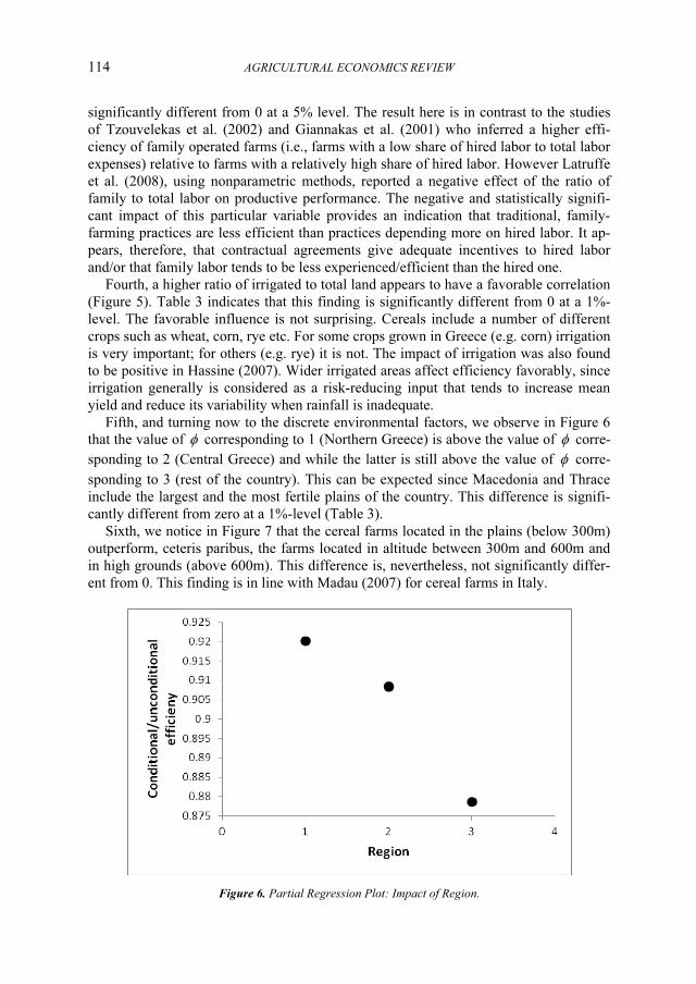
Fifth, and turning now to the discrete environmental factors, we observe in Figure 6
that the value of φ corresponding to 1 (Northern Greece) is above the value of φ corre-
sponding to 2 (Central Greece) and while the latter is still above the value of φ corre-
sponding to 3 (rest of the country). This can be expected since Macedonia and Thrace
include the largest and the most fertile plains of the country. This difference is signifi-
cantly different from zero at a 1%-level (Table 3).
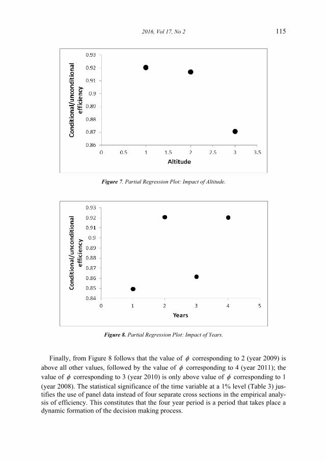
Sixth, we notice in Figure 7 that the cereal farms located in the plains (below 300m)
outperform, ceteris paribus, the farms located in altitude between 300m and 600m and
in high grounds (above 600m). This difference is, nevertheless, not significantly differ-
ent from 0. This finding is in line with Madau (2007) for cereal farms in Italy.
Figure 6. Partial Regression Plot: Impact of Region.
2016, Vol 17, �o 2 115
Figure 7. Partial Regression Plot: Impact of Altitude.
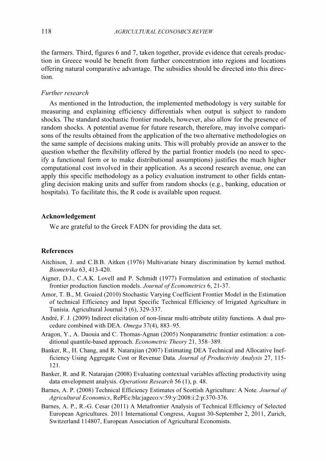
Figure 8. Partial Regression Plot: Impact of Years.
Finally, from Figure 8 follows that the value of φ corresponding to 2 (year 2009) is
above all other values, followed by the value of φ corresponding to 4 (year 2011); the
value of φ corresponding to 3 (year 2010) is only above value of φ corresponding to 1
(year 2008). The statistical significance of the time variable at a 1% level (Table 3) jus-
tifies the use of panel data instead of four separate cross sections in the empirical analy-
sis of efficiency. This constitutes that the four year period is a period that takes place a
dynamic formation of the decision making process.

116 AGRICULTURAL ECO�OMICS REVIEW
Table 3. �onparametric Significance Tests
p-value
Impact as Revealed
from the Partial
Regression Plot
Conclusion
(using the p-value and the evidence
from the partial regression plot)
Owners’
Age 0.384 Favorable
No statistically significant effect of
the owner’s age on productive per-
formance
Owned to
Total Land 0.046 ** Unfavorable
Negative and statistically significant
effect of the ratio of owned to total
land on productive performance
Family to
Total La-
bor
0.032 ** Unfavorable
Negative and statistically significant
effect of the ratio of family to total
labor on productive performance
Irrigated to
Total Land <2e-16 * Favorable
Positive and statistically significant
effect of the ratio of irrigated to total
land on productive performance
Year <2e-16 * Year 2009 is favorable Positive and statistically significant
effect of the year 2009
Region 0.001 * Location in Northern
Greece is favorable
Positive and statistically significant
effect of a Northern region on produc-
tive performance
Altitude 0.250 Location in altitude <
300m is favorable
No statistically significant effect of
altitude on productive performance
Where * (**) (***) denotes statistically significant at the 1% (5%) (10%) level, respectively
4. Conclusions and Policy Implications
EU faces the challenge of a new economic environment, of climate- related and
technological changes but also diversity in agriculture between Member States. Under
this context, the EU 2020 strategy regarding the CAP should take into account these
perspectives. An option suggested by the European Commission involves a shift from
the present status (different level of aid per country) towards an EU average with the
same level of aid per hectare in each EU country. This policy is unfavorable for those
countries that now are situated above the EU average aid (as is Greece). In addition,
there is a significant deviation between the agricultural input-output prices. Insights in
the relative efficiency could allow managers and policy makers to offset the potential
losses, exploiting utmost the given resources.
In this context, the present work investigates the performance of cereal farms in
Greece using panel data from the FADN of the EU. We examine relative efficiency by a
recently developed fully nonparametric robust partial frontier technique: the α -quantile
estimator. We apply a procedure to allow for the inclusion of mixed (both continuous
and discrete) environmental/exogenous variables. This so-called ‘conditional α -
quantile estimator’ is convenient for the setting at hand as (1) it does not require an a

2016, Vol 17, �o 2 117
priori specification on the agricultural production function, (2) mitigates the influence of
random shocks (e.g., due to weather) and (3) allows us to examine the correlation with
farm-specific factors which influence the relative efficiency scores.
The results can be structured along three lines. First, the unconditional estimates in-
dicate considerable efficiency differentials among the 632 farms in the sample. 15.98%
of the firms are classified as very inefficient, 10.44% are classified as ‘super-efficient’
and 32.12% lie on the respective unconditional a-quantile frontiers. The conditional
estimates, however, suggest that a large part of the efficiency differentials disappear
once the operational environment is accounted for. Indeed, on the basis of the condi-
tional estimates, 94.94% lie on the respective conditional a-quantile frontiers while no
farms are classified as ‘super-efficient’.
Second we reveal which control variables have a significant influence on efficiency.
On the basis of partial regression plots, the ratio of owned to total land and of family to
total labor appeared to have an unfavorable impact on productive performance, while
the farmer’s age, the ratio of irrigated to total land, the location in the Northern regions
and in low altitude appeared to have a favorable impact. Also farms from year 2009
outperform farms from all other years. Nevertheless, for only five of the above envi-
ronmental/exogenous factors the effect is statistically significance at the conventional
levels. Taken together, the nonparametric regression plots and the significance tests ap-
pear to suggest that irrigation and concentration of production to regions and locations
offering natural comparative advantage would benefit the sector. The same is true for
the lower ratio of owned to total land and of family to total labor. The time variable in-
cluded in the empirical analysis turned out to be statistically significant suggesting that
efficiency in cereal farms in Greece is not constant but it may changes from one period
to another.
Third, some of our results are different from previous studies that followed paramet-
ric estimations. We observed different finding regarding the unfavorable impact of the
ratio of family to total labor on a farm’s productive performance which is in contrast
with the findings of Tzouvelekas et al. (2002) and Giannakas et al. (2001). Also the un-
favorable influence on efficiency of the ratio of owned to total land reported here is dif-
ferent with earlier parametric literature findings (Tzouvelekas et al., 2002; Barnes,
2008). These differences may arise from the parametric assumptions made in earlier
studies.
Policy implications
This paper has three major policy implications. First, rural development programs for
cereals production should at least compensate for the firm-specific variables which have
been shown to influence efficiency. The robust theory used here reveals which variables
have a positive or negative effect on efficiency. Programs focused on rural development
could accordingly compensate for the unfavorable or the favorable environment depend-
ing on the policy priorities. This implies a utilitarian approach for policy implementa-
tion.
Second, the results indicate that family labor tends to be less experienced/efficient
than hired one. Hired labour might be more qualified and more able to perform special-
ized tasks than family labor. This justifies the funding of education and training pro-
grams for family members or the development of a consultant and advisory network for
118 AGRICULTURAL ECO�OMICS REVIEW
the farmers. Third, figures 6 and 7, taken together, provide evidence that cereals produc-
tion in Greece would be benefit from further concentration into regions and locations
offering natural comparative advantage. The subsidies should be directed into this direc-
tion.
Further research
As mentioned in the Introduction, the implemented methodology is very suitable for
measuring and explaining efficiency differentials when output is subject to random
shocks. The standard stochastic frontier models, however, also allow for the presence of
random shocks. A potential avenue for future research, therefore, may involve compari-
sons of the results obtained from the application of the two alternative methodologies on
the same sample of decisions making units. This will probably provide an answer to the
question whether the flexibility offered by the partial frontier models (no need to spec-
ify a functional form or to make distributional assumptions) justifies the much higher
computational cost involved in their application. As a second research avenue, one can
apply this specific methodology as a policy evaluation instrument to other fields entan-
gling decision making units and suffer from random shocks (e.g., banking, education or
hospitals). To facilitate this, the R code is available upon request.
Acknowledgement
We are grateful to the Greek FADN for providing the data set.
References
Aitchison, J. and C.B.B. Aitken (1976) Multivariate binary discrimination by kernel method.
Biometrika 63, 413-420.
Aigner, D.J., C.A.K. Lovell and P. Schmidt (1977) Formulation and estimation of stochastic
frontier production function models. Journal of Econometrics 6, 21-37.
Amor, T. B., M. Goaied (2010) Stochastic Varying Coefficient Frontier Model in the Estimation
of technical Efficiency and Input Specific Technical Efficiency of Irrigated Agriculture in
Tunisia. Agricultural Journal 5 (6), 329-337.
André, F. J. (2009) Indirect elicitation of non-linear multi-attribute utility functions. A dual pro-
cedure combined with DEA. Omega 37(4), 883–95.
Aragon, Y., A. Daouia and C. Thomas-Agnan (2005) Nonparametric frontier estimation: a con-
ditional quantile-based approach. Econometric Theory 21, 358–389.
Banker, R., H. Chang, and R. Natarajian (2007) Estimating DEA Technical and Allocative Inef-
ficiency Using Aggregate Cost or Revenue Data. Journal of Productivity Analysis 27, 115-
121.
Banker, R. and R. Natarajan (2008) Evaluating contextual variables affecting productivity using
data envelopment analysis. Operations Research 56 (1), p. 48.
Barnes, A. P. (2008) Technical Efficiency Estimates of Scottish Agriculture: A Note. Journal of
Agricultural Economics, RePEc:bla:jageco:v:59:y:2008:i:2:p:370-376.
Barnes, A. P., R.-G. Cesar (2011) A Metafrontier Analysis of Technical Efficiency of Selected
European Agricultures. 2011 International Congress, August 30-September 2, 2011, Zurich,
Switzerland 114807, European Association of Agricultural Economists.
2016, Vol 17, �o 2 119
Battese, G.E., T.J. Coelli (1988) Prediction of firm-level technical efficiencies with a general-
ized frontier production function and panel data. Journal of Econometrics 3, 387–399.
Braverman, A., J. E. Stiglitz (1986) Cost-sharing arrangements under share cropping: Moral
hazard, incentive, flexibility and risk. American Journal of Agricultural Economics 68, 642–
52.
Bravo-Ureta, B., A. E. Pinheiro (1993) Efficiency Analysis of Developing Country Agriculture:
A Review of the Frontier Function Literature. Agricultural and Resource Economics Review,
22(1), 88-101.
Brummer, B. (2001) Estimating confidence intervals for technical efficiency: the case of private
farms in Slovenia. European Review of Agricultural Economics 28(3), 285–306.
Cazals, C., J.P. Florens, & L. Simar (2002) Nonparametric frontier estimation: A robust ap-
proach. Journal of Econometrics 1, 1–25.
Charnes, A., W.W. Cooper, E. Rhodes (1978) Measuring the efficiency of decision making
units. European Journal of Operations Research 2, 429– 444.
Cherchye, L., T. V. Puyenbroeck (2007) Profit efficiency analysis under limited information
with an application to German farm types. Omega 35(3), 335–49.
Daouia, D., L. Simar (2007) Nonparametric efficiency analysis: A multivariate conditional
quantile approach. Journal of Econometrics 140, 375-400.
Daraio, C., L. Simar (2005) Introducing environmental variables in nonparametric frontier mod-
els: a probabilistic approach. Journal of Productivity Analysis 24 (1), 93–121.
Daraio, C., L. Simar (2006) A robust nonparametric approach to evaluate and explain the per-
formance of mutual funds. European Journal of Operational Research 175, 516-542.
Daraio, C., L. Simar (2007) Advanced robust and nonparametric methods in efficiency analysis,
Methodology and applications. Series: Studies in Productivity and Efficiency, Springer.
Daraio, C., L. Simar, P.W. Wilson (2010) Testing Whether Two-Stage Estimation is Meaning-
ful in Nonparametric Models of Production, Discussion Paper #1031, Institut de Statistique,
UCL, Belgium.
De Witte, K. and M. Kortelainen (2013) What Explains Performance of Students in a Heteroge-
neous Environment? Conditional Efficiency Estimation with Continuous and Discrete Envi-
ronmental Variables. Applied Economics 45(17), 2401-2412.
Deprins, D., L. Simar, H. Tulkens (1984) Measuring labor efficiency in post offices. In M. Mar-
chand, P. Pestieau, & H. Tulkens (eds.). The Performance of Public Enterprises: Concepts
and Measurements, �orth-Holland, 243–267.
Dhehibi, B., H. Bahri, M. Annabi (2012) Input, Output Technical Efficiencies and Total Factor
Productivity of Cereal Production in Tunisia. 2012 Conference, August 18-24, 2012, Foz do
Iguacu, Brazil 122866, International Association of Agricultural Economists.
European Commission (2012), Directorate-General for Agriculture and Rural Development,
Agriculture in the European Union, Statistical and Economic information, Report, December
2012.
Galanopoulos, K., Z. Abas, V. Laga, I. Hatziminaoglou, J. Boyazoglu (2011). The technical
efficiency of transhumance sheep and goat farms and the effect of EU subsidies: Do small
farms benefit more than large farms? Small Ruminant Research 100, 1– 7
Gavian, S. and S. Ehui (1999) Measuring the Production Efficiency of Alternative Land Tenure
Contracts in a Mixed Crop-Livestock System in Ethiopia. Agricultural Economics 20. 37-49.
Giannakas, K., R. Schoney, V. Tzouvelekas (2001) Technical efficiency, technological change
and output growth of wheat farms in Saskatchewan. Canadian Journal of Agricultural Eco-
nomics 49, 135–152.
120 AGRICULTURAL ECO�OMICS REVIEW
Halkos, G.E., N.G. Tzeremes (2011) Modelling the Effect of National Culture on Multinational
Banks' Performance: A conditional Robust Nonparametric Frontier Analysis. Economic
Modelling 28(1-2), 515-525.
Hall, P., J. S. Racine, Q. Li (2004) Cross-validation and the estimation of conditional probabil-
ity densities. Journal of the American Statistical Association 99 (486), 1015–1026.
Hassine, N. B. (2007) Technical Efficiency In The Mediterranean Countries’ Agricultural Sec-
tor. Region et Developpement 25, 27-44.
Hayfield, T. and J.S. Racine (2008) Nonparametric econometrics: The np package. Journal of
Statistical Software 27 (5).
Jeong, S., B. Park and L. Simar (2008) Nonparametric conditional efficiency measures: Asymp-
totic properties. Annals of Operations Research, doi:10.1007/s10479-008-0359-5.
Kuosmanen, T., D. Pemsl, J. Wesseler (2006) Specification and estimation of production func-
tions involving damage control inputs: a two-stage, semiparametric approach. American
Journal of Agricultural Economics 88(2), 499–511.
Lansink, A. O., K. Pietola, S. Backman (2002) Efficiency and productivity of conventional and
organic farms in Finland 1994–1997. European Review of Agricultural Economics 29, 51–
65.
Larsen K, 2010. Effects of machinery-sharing arrangements on farm efficiency: evidence from
Sweden. Agricultural Economics. 41, 497–506.
Latruffe L, K. Balcombe, S. Davidova, K. Zawalinska (2004) Determinants of technical effi-
ciency of crop and livestock farms in Poland. Applied Economics 36(12), 1255–1263.
Latruffe, L., S. Davidova, K. Balcombe (2008) Application of a double bootstrap to investiga-
tion of determinants of technical efficiency of farms in Central Europe. Journal of Produc-
tivity Analysis 29, 183-191.
Latruffe, L., J. Fogarassy, Y. Desjeux (2012) Efficiency, productivity and technology compari-
son for farms in Central and Western Europe: The case of field crop and dairy farming in
Hungary and France. Economic Systems 36, 264–278.
Li, Q. and J.S. Racine (2007) Nonparametric econometrics: Theory and practice. Princeton
University Press.
Madau, F. (2007) Technical efficiency in organic and conventional farming: Evidence form
Italian cereal farms. Agricultural Economics Review 8 (1).
Mendes, A. B., E. L. D. G. Soares da Silva, A. Santos (2012) Efficiency Measures in the Agri-
cultural Sector. Jorge M (Eds.), Sringer.
Racine, J.S. (1997) Consistent significance testing for nonparametric regression. Journal of
Business and Economic Statistics 15 (3), 369-379.
Racine, J. S., J. Hart and Q. Li (2006) Testing the significance of categorical predictor variables
in nonparametric regression models. Econometric Reviews 25 (4), 523-544.
Scardera, A., R. Zanoli (eds.) L’agricoltura biologica in Italia. Rome: INEA.
Simar, L. and P. Wilson (2007) Estimation and inference in two-stage, semi-parametric models
of production processes. Journal of Econometrics 136 (1), 31.64.
Stevenson, R.E. (1980) Likelihood Functions for Generalized Stochastic Frontier Estimation.
Journal of Econometrics 13(1), 57-66.
Tavares, G (2009) A bibliography of date envelopment analysis:1978–2001. Socio-Economic
Planning Sciences 43(1), 72–88.
Thiele, H., C. M. Brodersen (1999) Differences in farm efficiency in market and transition
economies: empirical evidence from West and East Germany. European Review of Agricul-
tural Economics 26(3), 331–47.

2016, Vol 17, �o 2 121
Tzouvelekas, V., C.J. Pantzios, C. Fotopoulos (2002) Measuring multiple and single factor
technical efficiency in organic farming. The case of Greek wheat farms. British Food Jour-
nal 104 (8), 591-609.
Yatchew, A. (1998). Nonparametric regression techniques in economics. Journal of Economic
Literature, 36, 669-721.
Wheelock, D., P. Wilson (2008) Non-Parametric, Unconditional Quantile Estimation for Effi-
ciency Analysis with an Application to Federal Reserve Check Processing Operations. Jour-
nal of Econometrics, 14, 209–225.
Wheelock D., P. Wilson (2009) Robust Nonparametric Quantile Estimation of Efficiency and
Productivity Change in U.S. Commercial Banking, 1985–2004. Journal of Business & Eco-
nomic Statistics, 27(3), 354-368.
122 AGRICULTURAL ECO�OMICS REVIEW
TECH�ICAL APPE�DIX
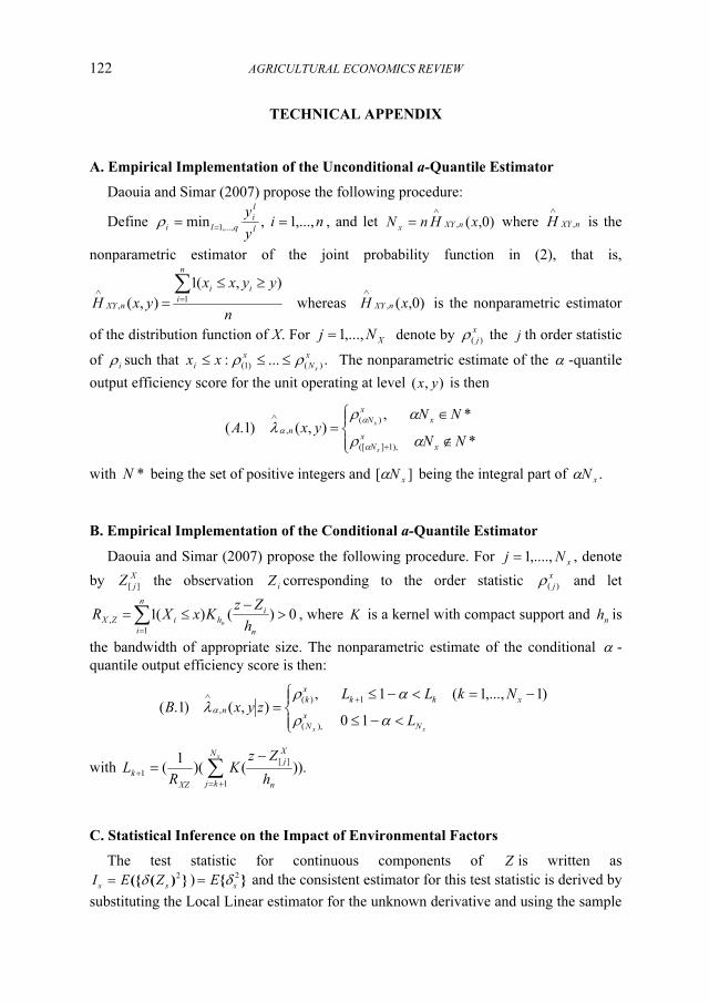
A. Empirical Implementation of the Unconditional a-Quantile Estimator
Daouia and Simar (2007) propose the following procedure:
Define niy
yl
l
i
qli ,...,1,min,...,1
===
ρ , and let )0,(, xHn� nXYx
∧
= where nXYH ,
∧
is the
nonparametric estimator of the joint probability function in (2), that is,
n
yyxx
yxH
n
i
ii
nXY
∑=
∧
≥≤
=1
,
),(1
),( whereas )0,(, xH nXY
∧
is the nonparametric estimator
of the distribution function of X. For X
�j ,...,1= denote by x
j )(ρ the j th order statistic
of i
ρ such that ....: )()1(
x
�
x
ix
xx ρρ ≤≤≤ The nonparametric estimate of the α -quantile
output efficiency score for the unit operating at level ),( yx is then
⎪⎩
⎪⎨⎧
∉
∈=
+
∧
*
*,),()1.(
),1]([
)(
,
��
��yxA
x
x
�
x
x
�
n
x
x
αρ
αρλ
α
α
α
with *� being the set of positive integers and ][x
�α being the integral part of .
x�α
B. Empirical Implementation of the Conditional a-Quantile Estimator
Daouia and Simar (2007) propose the following procedure. For x
�j ,....,1= , denote
by X
jZ ][ the observation i
Z corresponding to the order statistic x
j )(ρ and let
0)()(11
,>
−≤=∑
= n
i
h
n
i
iZX
h
ZzKxXR
n
, where K is a kernel with compact support and n
h is
the bandwidth of appropriate size. The nonparametric estimate of the conditional α -
quantile output efficiency score is then:
⎪⎩
⎪⎨⎧
<−≤
−=<−≤=
+∧
xx�
x
�
xkk
x
k
n
L
�kLLzyxB
αρ
αρλα
10
)1,...,1(1,),()1.(
),(
1)(
,
with ∑+=
+
−
=
x�
kj n
X
j
XZ
kh
ZzK
RL
1
][
1 )).()(1
(
C. Statistical Inference on the Impact of Environmental Factors
The test statistic for continuous components of Z is written as
})(({2
ssZEI δ= ) }{
2
sE δ= and the consistent estimator for this test statistic is derived by
substituting the Local Linear estimator for the unknown derivative and using the sample
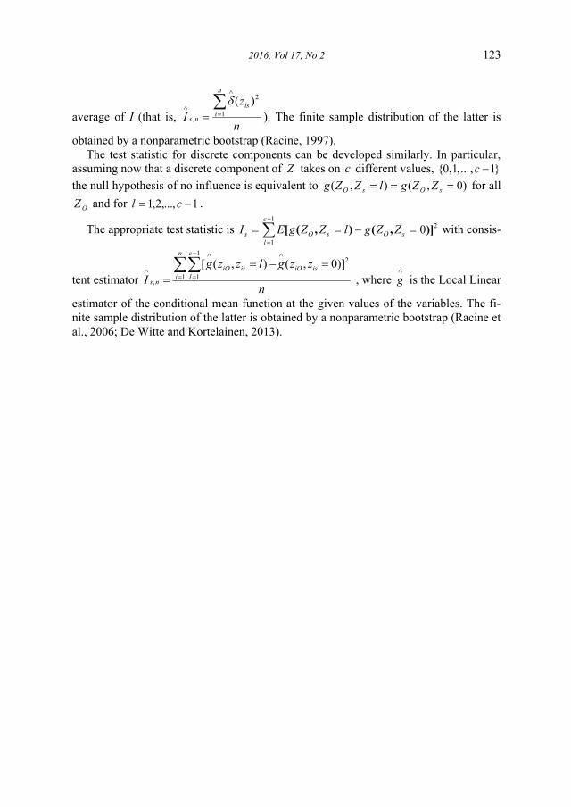
2016, Vol 17, �o 2 123
average of I (that is, n
z
I
n
i
is
ns
∑=
∧
∧
=
1
2
,
)(δ
). The finite sample distribution of the latter is
obtained by a nonparametric bootstrap (Racine, 1997).
The test statistic for discrete components can be developed similarly. In particular,
assuming now that a discrete component of Z takes on c different values, }1,...,1,0{ −c
the null hypothesis of no influence is equivalent to )0,(),( ===sOsO
ZZglZZg for all
OZ and for 1,...,2,1 −= cl .
The appropriate test statistic is 2
1
1
0)],(),([ =−==∑−
=
sO
c
l
sOsZZglZZgEI with consis-
tent estimator n
zzglzzg
IisiO
n
i
isiO
c
lns
2
1
1
1,
)]0,(),([ =−=
=
∧
=
−
=
∧
∧∑∑
, where ∧
g is the Local Linear
estimator of the conditional mean function at the given values of the variables. The fi-
nite sample distribution of the latter is obtained by a nonparametric bootstrap (Racine et
al., 2006; De Witte and Kortelainen, 2013).