Etude du comportement à la rupture d'un matériau fragile ...

Effets du taux de deformation sur la rupture ductile des
aciers a haute performance : Experiences et modelisation
Matthieu Dunand
To cite this version:
Matthieu Dunand. Effets du taux de deformation sur la rupture ductile des aciers a hauteperformance : Experiences et modelisation. Mecanique des solides [physics.class-ph]. EcolePolytechnique X, 2013. Francais. <pastel-00838906>
HAL Id: pastel-00838906
https://pastel.archives-ouvertes.fr/pastel-00838906
Submitted on 26 Jun 2013
HAL is a multi-disciplinary open accessarchive for the deposit and dissemination of sci-entific research documents, whether they are pub-lished or not. The documents may come fromteaching and research institutions in France orabroad, or from public or private research centers.
L’archive ouverte pluridisciplinaire HAL, estdestinee au depot et a la diffusion de documentsscientifiques de niveau recherche, publies ou non,emanant des etablissements d’enseignement et derecherche francais ou etrangers, des laboratoirespublics ou prives.

Thèse présentée pour obtenir le grade de
DOCTEUR DE L’ECOLE POLYTECHNIQUE
Spécialité : Mécanique
Par
MATTHIEU DUNAND
Effect of strain rate on the ductile fracture of
Advanced High Strength Steel Sheets:
Experiments and modeling
Soutenue le 25 juin 2013, devant le jury composé de :
Alexis RUSINEK LaBPS, ENIM Président
Tore BØRVIK SIMLab, NTNU Rapporteur
Vincent GROLLEAU LIMB, Univ. Bretagne Sud Rapporteur
Patricia VERLEYSEN Universiteit Gent Examinatrice
Han ZHAO LMT, ENS Cachan Examinateur
Gérard GARY LMS, Ecole Polytechnique Encadrant
Dirk MOHR LMS, Ecole Polytechnique Directeur de thèse


Résumé
L’industrie automobile emploie massivement les Aciers à Haute Performance
(AHP) pour la fabrication des caisses en blanc, en raison de leur rapport
résistance/masse élevé. Ils sont utilisés afin d’augmenter la sécurité des occupants en
cas de crash, ou de réduire la masse du véhicule grâce à une diminution des sections
utiles. En parallèle, le prototypage virtuel est omniprésent dans le processus de
conception des nouveaux véhicules. En prenant l’exemple d’une caisse en blanc
automobile, la conception de la structure globale et des procédés de mise en forme de
ses composants nécessite des modèles prédictifs et fiables décrivant le comportement et
la rupture des matériaux utilisés. Des efforts soutenus ont été entrepris ces cinq
dernières années pour développer des modèles prédisant la rupture des AHP sous
chargement statique. Pourtant les taux de déformations rencontrés lors d’opération de
mise en forme sont de l’ordre de 10 s-1
, et peuvent atteindre 103 s
-1 lors de crashs.
Le but de cette thèse est de développer une méthode fiable permettant d’évaluer
l’influence du taux de déformation et de l’état de contrainte sur la rupture ductile
d’AHP initialement non-fissurés. Une procédure expérimentale est conçue pour
caractériser le comportement et l’initiation de la rupture dans des tôles chargées en
traction à grande vitesse de déformation. La précision du dispositif est évaluée grâce à
des validations numériques et expérimentales. Par la suite, une série d’expériences est
réalisée à petite, moyenne et grande vitesse de déformation sur différents types
d’éprouvettes de traction, afin de couvrir un spectre étendu d’états de contraintes. Une
analyse détaillée de chaque expérience par la méthode des Éléments Finis permet de
déterminer le trajet de chargement et l’état de déformation et de contrainte à la rupture
dans chaque éprouvette, tout en prenant en compte les phénomènes de striction. La
déformation à la rupture est significativement plus élevée à grande vitesse de
déformation qu’à basse vitesse. De plus, les résultats montrent que l’influence du taux
de déformation sur la ductilité ne peut pas être découplée de l’état de contrainte.
Le modèle de comportement constitue un élément essentiel de cette approche
hybride expérimentale-numérique. Un modèle de plasticité dépendant du taux de

ii
déformation est proposé pour prédire la réponse mécanique des AHP sur toute la plage
de déformation, taux de déformation et état de contrainte couverte par le programme
expérimental. La précision du modèle est validée par comparaison de mesures
expérimentales globales et locales aux prédictions numériques correspondantes. De
plus, l’influence de la discrétisation spatiale utilisée dans les simulations par Eléments
Finis sur la précision de l’approche hybride expérimentale-numérique est quantifiée. Il
est montré qu’un maillage fin d’éléments hexaédriques est nécessaire pour obtenir des
prédictions précises jusqu’à la rupture. Ce type de maillage n’est pas compatible avec
des applications industrielles à grande échelle pour des raisons évidentes d’efficacité
numérique. C’est pourquoi une méthode de remaillage dynamique d’éléments coque
vers des éléments solides est présentée et évaluée. Cette méthode permet d’obtenir des
prédictions fiables de l’initiation de la rupture dans des tôles sans compromettre
dramatiquement l’efficacité numérique obtenue grâce aux éléments coque.
La seconde partie de ce travail s’intéresse aux micro-mécanismes responsables de
la rupture ductile du matériau étudié. Une analyse micrographique du matériau soumis
à différents niveaux de déformation permet d’identifier l’enchainement des mécanismes
d’endommagement. Ces observations suggèrent que le mécanisme critique conduisant à
la rupture est la localisation de la déformation plastique dans une bande de cisaillement
à l’échelle du grain. Un model numérique reposant sur la déformation d’une cellule
élémentaire 3D contenant une cavité est développé pour modéliser ce phénomène. Il est
montré que le mécanisme de localisation à l’échelle micro de l’écoulement plastique
dans une bande de cisaillement permet d’expliquer la dépendance de la ductilité à l’état
de contrainte et au taux de déformation observée à l’échelle macro.

Acknowledgement


Contents
Résumé .................................................................................................. i
Acknowledgement .............................................................................. iii
Contents ............................................................................................... v
List of figures ...................................................................................... ix
List of Tables ..................................................................................... xv
1. General introduction .......................................................................... 1
1.1 Industrial context .................................................................................. 1
1.2 Objective and structure of the thesis ................................................... 2
1.3 Material .................................................................................................. 5
2. Preliminaries ....................................................................................... 7
2.1 Characterization of the stress state ...................................................... 7
2.1.1 Stress invariants .......................................................................... 7
2.1.2 Plane stress condition ................................................................ 10
2.2 Ductile fracture modeling ................................................................... 12
2.3 Rate-independent plasticity of AHSS ................................................ 15
2.4 Split Hopkinson Pressure bar systems .............................................. 18
3. High strain rate tensile experiments ............................................... 21
3.1 Introduction ......................................................................................... 22
3.2 Load inversion device .......................................................................... 27
3.2.1 Design objective and strategy ................................................... 27
3.2.2 Proposed design ........................................................................ 29
3.3 Experimental procedure ..................................................................... 31
3.3.1 Split Hopkinson Pressure Bar (SHPB) system .......................... 31
3.3.2 Forces and velocities at the specimen boundaries ..................... 32
3.3.3 Local displacement measurements ............................................ 34
3.3.4 Determination of the stress-strain curve ................................... 34
3.4 FEA-based validation .......................................................................... 35
3.4.1 Finite element model ................................................................. 36

vi
3.4.2 Simulation results ...................................................................... 37
3.5 Validation experiments ....................................................................... 41
3.5.1 High strain rate uniaxial tension experiments ........................... 41
3.5.2 Notched tension experiments .................................................... 48
3.6 Conclusions .......................................................................................... 50
4. Hybrid experimental-numerical characterization of the effect
of strain rate on fracture .................................................................. 53
4.1 Introduction ......................................................................................... 54
4.2 Experimental program ....................................................................... 58
4.2.1 Tensile experiments at low and intermediate strain rate ........... 58
4.2.2 Tensile experiments at high strain rate ..................................... 58
4.2.3 Local displacements and strain measurements ......................... 60
4.3 Experimental results ........................................................................... 61
4.3.1 Uniaxial tension ........................................................................ 61
4.3.2 Notched tension ........................................................................ 63
4.4 Rate- and temperature-dependent plasticity modeling ................... 66
4.4.1 Constitutive equations ............................................................... 66
4.4.2 Model specialization ................................................................. 68
4.4.3 Calibration procedure ................................................................ 72
4.5 Numerical analysis and plasticity model validation ......................... 76
4.5.1 Finite element model ................................................................. 76
4.5.2 Comparison of numerical and experimental results .................. 79
4.6 Loading histories to fracture .............................................................. 80
4.7 Conclusion ............................................................................................ 86
5. Numerical methods for accurate and efficient ductile fracture
predictions ......................................................................................... 87
5.1 Introduction ......................................................................................... 88
5.2 An uncoupled fracture model for Advanced High Strength Steel
sheets .................................................................................................... 89
5.2.1 Plasticity model ......................................................................... 89
5.2.2 Fracture model .......................................................................... 90
5.3 Influence of Finite Element modeling on ductile fracture
predictions ............................................................................................ 91
5.3.1 Methodology ............................................................................. 93
5.3.2 Results for shell elements ......................................................... 94
5.3.3 Results for solid elements ......................................................... 97

vii
5.3.4 Comparison shell-solid ............................................................ 100
5.3.5 Mixed shell-solid model .......................................................... 102
5.4 Dynamic shell-to-solid re-meshing ................................................... 105
5.4.1 Principle .................................................................................. 105
5.4.2 Simple example ....................................................................... 107
5.4.3 Application to basic fracture experiments ............................... 110
5.5 Conclusion .......................................................................................... 118
6. Analysis of the failure micro-mechanisms ................................... 121
6.1 Introduction ....................................................................................... 122
6.2 Macroscopic analysis: experiments and simulations ..................... 122
6.2.1 Notched tension experiments .................................................. 123
6.2.2 Tension on a specimen with a central hole ............................. 126
6.2.3 Punch Experiment ................................................................... 129
6.2.4 Dependence of the strain to fracture on stress state ................ 129
6.3 Fractographic analysis ...................................................................... 130
6.3.1 Sample preparation .................................................................. 130
6.3.2 Microscopic observations of polished cross-sections ............. 131
6.3.3 Fracture surfaces ..................................................................... 137
6.3.4 Effect of strain rate on damage ............................................... 137
6.4 Mechanical interpretation of the observations ............................... 137
6.5 Conclusion .......................................................................................... 139
7. Modeling of the failure mechanisms ............................................. 141
7.1 Introduction ....................................................................................... 142
7.2 Micromechanical modeling .............................................................. 146
7.2.1 3D unit cell model geometry and boundary conditions .......... 147
7.2.2 Macroscopic rate of deformation tensor.................................. 149
7.2.3 Control of the macroscopic stress state ................................... 150
7.2.4 Stress orientation evolution ..................................................... 153
7.2.5 Computation of the onset of localization for a given stress
state ......................................................................................... 154
7.3 Simulation results .............................................................................. 155
7.3.1 Onset of localization ............................................................... 155
7.3.2 Effect of anisotropy ................................................................. 159
7.3.3 Influence of the biaxial stress ratio on localization ................. 162
7.3.4 Influence of the defect volume fraction .................................. 164

viii
7.4 Rate-dependent localization analysis .............................................. 166
7.5 Conclusion .......................................................................................... 170
8. Conclusion ....................................................................................... 171
8.1 Summary of the contributions ......................................................... 171
8.2 Future research ................................................................................. 173
8.2.1 High strain rate experiments ................................................... 173
8.2.2 Influence of temperature ......................................................... 175
8.2.3 Rate-dependent fracture model ............................................... 176
8.2.4 Rate-dependent localization analysis ...................................... 177
A. Numerical implementation of the rate-dependent plasticity
model ............................................................................................... 179
A.1 Time integration scheme .................................................................. 179
A.1.1 Isothermal loading .................................................................. 180
A.1.2 Adiabatic loading .................................................................... 181
A.1.3 First guess for the Newtown algorithm ................................... 182
A.1.4 Explicit FEA solver ................................................................. 182
A.2 Material Jacobian ............................................................................. 183
A.2.1 Isothermal loading .................................................................. 183
A.2.2 Adiabatic loading .................................................................... 185
A.3 Material derivatives .......................................................................... 186
A.3.1 Yield and flow potentials and .......................................... 187
A.3.2 Strain rate function .............................................................. 187
A.3.3 Strain hardening function .................................................... 188
B. Publications & Presentations ......................................................... 191
B.1 Refereed journal publications .......................................................... 191
B.2 Conference proceedings .................................................................... 192
B.3 Presentations ...................................................................................... 193
Bibliography .................................................................................... 197

List of figures
Figure 1-1: Optical micrograph of the undeformed TRIP material. ................................ 6
Figure 2-1: Characterization of the stress states in terms of stress triaxiality and
Lode angle parameter. ............................................................................................... 9
Figure 2-2: Relation between the stress triaxiality , the Lode angle parameter
and the stress ratio in case of biaxial stress states. ............................................... 11
Figure 2-3: Uniaxial tensile testing – engineering stress strain ..................................... 17
Figure 2-4: Schematic of a Split Hopkinson Pressure Bar system ................................ 18
Figure 2-5: Wave-propagation diagram ......................................................................... 18
Figure 2-6: Example of signals measured in a SHPB experiment ................................. 19
Figure 3-1: Configurations for tensile testing with SHPB systems. .............................. 23
Figure 3-2: Schematic of the Load Inverting Device .................................................... 30
Figure 3-3: Drawings of the specimens ......................................................................... 31
Figure 3-4: Results from a FE simulation of a uniaxial tension experiment ................. 38
Figure 3-5: Displacement of two nodes located on the surface of the specimen gage
section ...................................................................................................................... 39
Figure 3-6: FE-based validation of the experimental technique for uniaxial tension .... 40
Figure 3-7: Photograph of the load inversion device ..................................................... 41
Figure 3-8: Close-up view of a notched specimen positioned in the load inversion
device. ...................................................................................................................... 42
Figure 3-9: Strain histories of (a) the incident and reflected wave measured from the
input bar and (b) the transmitted waves measured from both output bars ............... 43
Figure 3-10: Approximation of the forces applied at the specimen/pusher interface .... 44
Figure 3-11: Axial engineering strain distribution along the specimen gage section .... 45

x
Figure 3-12: Summary of experimental results for different equivalent plastic strain
rates. .......................................................................................................................... 46
Figure 3-13: True stress-strain curves ............................................................................ 48
Figure 3-14: Experiments on a notched tensile specimen. ............................................. 49
Figure 4-1: Uniaxial tension specimens ......................................................................... 59
Figure 4-2: Experimental engineering stress-strain curves under uniaxial tension. ....... 62
Figure 4-3: Experimental results of notched tensile specimens with a 20mm radius. ... 64
Figure 4-4: Experimental results of notched tensile specimens with a 6.65mm
radius. ....................................................................................................................... 65
Figure 4-5: Dependence of flow stress to temperature ................................................... 71
Figure 4-6: Experimental (points) and simulation (solid curves) results for the
notched tensile specimen with a radius, at (a) low, (b)
intermediate and (c) high strain rate. ........................................................................ 75
Figure 4-7: Experimental (points) and simulation (solid curves) results for uniaxial
tension ....................................................................................................................... 77
Figure 4-8: Experimental (points) and simulation (solid curves) results for the
notched tensile specimen with a radius, at (a) low, (b) intermediate
and (c) high strain rate. ............................................................................................. 79
Figure 4-9: Numerical prediction of the evolution of equivalent plastic strain rate
versus equivalent plastic strain ................................................................................. 83
Figure 4-10: Loading path in the plane for low strain rate experiments. ................ 84
Figure 4-11: Loading paths to fracture at low (black lines), intermediate (red lines)
and high strain rate (blue lines). ............................................................................... 85
Figure 5-1: Meshes of the notched tensile specimen. ..................................................... 92
Figure 5-2: View of the very fine mesh with 12 solid elements through the half-
thickness ................................................................................................................... 93
Figure 5-3: Predicted force displacement curves with shell elements............................ 95

xi
Figure 5-4: Evolution of damage and equivalent plastic strain at the center of the
notched specimen ..................................................................................................... 95
Figure 5-5: Contour plot of equivalent plastic strain after the maximum of force ........ 96
Figure 5-6: Evolution of the stress triaxiality and the equivalent plastic strain ............ 97
Figure 5-7: Predicted force displacement curves with solid elements. ......................... 98
Figure 5-8: Evolution of the equivalent plastic strain at the center of the gage
section for different mesh densities. ........................................................................ 98
Figure 5-9: Contour plot of equivalent plastic strain after the onset of localized
necking ..................................................................................................................... 99
Figure 5-10: Predicted displacement at which fracture occurs .................................... 101
Figure 5-11: Mixed mesh with local refinement of solid elements. ............................ 103
Figure 5-12: Force displacement curves and fracture predictions using a solid mesh
and a mixed mesh. ................................................................................................. 103
Figure 5-13: Evolution of equivalent plastic strain (solid lines) and stress triaxiality
(dashed lines) at the center of the gage section ..................................................... 104
Figure 5-14: Simulation of a tension test using shell-to-solid re-meshing. ................. 106
Figure 5-15: Force displacement curve of a tensile test with re-meshing ................... 109
Figure 5-16: Evolution of the model kinetic energy .................................................... 109
Figure 5-17: Flat tensile specimens with different notched radii and with a central
hole. ....................................................................................................................... 111
Figure 5-18: Contour plot of equivalent plastic strain in a notched tensile
specimen after re-meshing of the gage section center. .......................................... 112
Figure 5-19: Predicted force displacement curve of the notched tensile test
with re-meshing. .................................................................................................... 113
Figure 5-20: Predicted force displacement curve of the notched tensile test
with re-meshing. .................................................................................................... 113
Figure 5-21: Predicted force displacement curve of the central hole tensile test with
re-meshing. ............................................................................................................ 114

xii
Figure 5-22: Evolution of equivalent plastic strain at the center of the
notched tensile specimen, predicted using a solid mesh or re-meshing. ................ 115
Figure 5-23: Evolution of stress triaxiality at the center of the notched
tensile specimen, predicted using a solid mesh or re-meshing. .............................. 116
Figure 5-24: Evolution of damage at the center of the notched tensile
specimen, predicted using a solid mesh or re-meshing. ......................................... 116
Figure 6-1: Tensile specimens with (a) a notch radius 6.65mm and (b) tensile
specimen with central hole. .................................................................................... 123
Figure 6-2: Force displacement curves ......................................................................... 125
Figure 6-3: Contour plot of the equivalent plastic strain at the instant of the onset of
fracture in a notched specimen. .............................................................................. 126
Figure 6-4: Loading paths to fracture. .......................................................................... 127
Figure 6-5: Specimen with a central hole: contour plot of plastic axial strain at the
instant of the onset of fracture. ............................................................................... 128
Figure 6-6: SEM micrographs from notched tensile experiments interrupted at (a)
the maximum of force, (b) 95% of the displacement to fracture and (c) 99% of
the displacement to fracture. ................................................................................... 133
Figure 6-7: Cross sections of post-mortem specimens of (a) notched tensile
experiment, (b) central hole experiment and (c) punch experiment. ...................... 135
Figure 6-8: SEM fractographs from a broken notched tensile specimen. .................... 136
Figure 7-1: (a) unit cell initial geometry and (b) FEA mesh representing half of the
cell. ......................................................................................................................... 146
Figure 7-2: Unit cell model in its (a) initial and (b) deformed configuration. ............. 151
Figure 7-3: Contour plot of equivalent plastic strain in the plane .................... 156
Figure 7-4: Influence of initial stress orientation on the onset of localization for
. .................................................................................................................. 159
Figure 7-5: Cavity shape evolution during deformation under uniaxial tension
. ..................................................................................................................... 161

xiii
Figure 7-6: Dependence of (a) the macroscopic strain and (b) the stress
orientation at the onset of localization to the biaxial stress ratio . ................ 163
Figure 7-7: Influence of the initial defect volume fraction on (a) macroscopic stress-
strain curves and (b) the evolution of the defect volume fraction for a biaxial
stress ratio of . .......................................................................................... 165
Figure 7-8: Evolution of the macroscopic equivalent strain rate in rate dependent
cell calculations. .................................................................................................... 167
Figure 7-9: Influence of strain rate on localization for a biaxial stress ratio of
. ................................................................................................................. 168
Figure 8-1: Scatter in high velocity equi-biaxial punch experiments. ......................... 174
Figure 8-2: Isothermal uniaxial tension experiments at different temperatures. ......... 176


List of Tables
Table 1-1: Chemical composition of the TRIP780 material in wt-% .............................. 5
Table 4-1: Material parameters for the rate-dependent model ...................................... 73
Table 5-1: Material parameters for the TRIP780 steel .................................................. 92
Table 5-2: CPU time (in s) for different mesh types and densities ............................. 100
Table 5-3: CPU time (in s) for the solid and mixed models ........................................ 105
Table 5-4: CPU time (in s) when using re-meshing .................................................... 118
Table 7-1: Material parameters used for rate-dependent cell calculations .................. 166

Chapter 1
General introduction
Contents
1.1 Industrial context ............................................................................................. 1
1.2 Objective and structure of the thesis ................................................................ 2
1.3 Material ............................................................................................................ 5
1.1 Industrial context
The automotive industry has widely incorporated Advanced High Strength Steels
sheets (AHSS) in vehicle structures due to their high strength to weight ratio: they are
used to improve the vehicle safety or to reduce the vehicle weight through the use of
thinner gages. At the same time, new vehicle design relies heavily on virtual
prototyping practices. In the specific example of automotive structures, both the
engineering of the production process and of the final product require reliable models
of plasticity and fracture. Consequently, great efforts have been undertaken during the
last five years to develop models that can predict the fracture of AHSS under static
conditions (e.g. Wierzbicki et al., 2010, [190]). However, rates of deformation
encountered in sheet metal forming operations are typically of the order of 10s-1
, while
they can be as high as 103
s-1
under accidental crash loading. Therefore, there is a need
to investigate the effect of strain rate on deformation behavior and fracture of AHSS,
and to assess whether models developed for static loading conditions can satisfactorily
be used in industrial applications.

2 Chapter 1. General introduction
1.2 Objective and structure of the thesis
This project was carried out in collaboration between the Solid Mechanics
Laboratory (CNRS-UMR 7649, Ecole Polytechnique) and the Impact and
Crashworthiness Laboratory (Massachusetts Institute of Technology).
The present research work consists of two main parts. The first part aims at
developing a reliable methodology for evaluating the influence of strain rate as well as
stress state on the ductile fracture properties of initially uncracked Advanced High
Strength Steel sheets. An experimental procedure is designed to characterize the
deformation behavior and the onset of fracture of sheet materials under tensile loading
at high strain rate. Numerical and experimental validations of the proposed setup are
performed to evaluate its accuracy. Then an experimental program is carried out at low,
intermediate and high strain rates on different type of tensile specimens, thereby
covering a range of stress states. Detailed Finite Element analyses of each experiment
are used to determine the loading history and the material state at fracture in each
experiment. A key component of this hybrid experimental-numerical approach is the
constitutive model: a rate-dependent plasticity model is proposed to predict the
mechanical response of AHSS over all the range of strains, strain rates and stress states
reached in the experiments. The model accuracy is validated by comparing global and
local test measurements to the corresponding simulation predictions. In addition, the
influence of the geometric discretization used in Finite Element analysis on the
accuracy of the hybrid experimental-numerical approach is evaluated. It is shown that
fine meshes of brick elements are required for accurate fracture predictions, but cannot
be used in industrial applications because of inadequate computational efficiency. A
technique of shell-to-solid re-meshing is presented and evaluated, that allows for
accurate predictions of the onset of ductile fracture in sheet materials without
compromising the numerical efficiency of shell elements.
The second part of this work is concerned with the micro-mechanisms
responsible for ductile failure. Micrographs of specimens corresponding to different
stages of loading prior to failure are analyzed to identify the sequence of damage
processes leading to fracture. Observations suggest that the governing failure
mechanism is the localization of plastic deformation into shear bands at the grain level.

1.2. Objective and structure of the thesis 3
A numerical model based on three dimensional unit cell calculations is developed to
assess whether the mechanism of shear localization of the plastic flow at the micro-
scale can explain the dependence of the material ductility to both stress state and strain
rate that was observed at the macro-scale.
The thesis is organized as follow:
In Chapter 2, background information is given on the characterization and
modeling of plasticity and ductile fracture of AHSS under static loading conditions. In
addition, variables that will be used throughout the manuscript to describe the stress
state are precisely defined. Finally, Split Hopkinson Pressure Bar systems, used for
characterizing mechanical behavior of materials under compression at high rates of
deformation, are presented.
In Chapter 3, a high strain rate tensile testing technique for sheet materials is
presented which makes use of a modified split Hopkinson pressure bar system in
conjunction with a load inversion device. With compressive loads applied to its
boundaries, the load inversion device introduces tension into a sheet specimen. Detailed
finite element analysis of the experimental set-up is performed to validate the design of
the load inversion device. It is shown that under the assumption of perfect alignment
and slip-free attachment of the specimen, the measured stress-strain curve is free from
spurious oscillations at a strain rate of 1000s-1
. Validation experiments are carried out
using tensile specimens, confirming the oscillation-free numerical results in an
approximate manner.
In Chapter 4, the effect of strain rate on ductile fracture properties of the TRIP
material is characterized using a hybrid experimental-numerical method. Tensile
experiments are carried out at low ( ), intermediate ( ) and high strain
rates ( ). The experimental program includes notched as well as uniaxial
tension specimens. Local displacements and surface strain fields are measured optically
in all experiments using Digital Image Correlation. Constitutive equations derived from
the Mechanical Threshold Stress theory are proposed to describe the rate-dependent
behavior as well as plastic anisotropy of the sheet material. Detailed Finite Element
simulations of all experiments reveal that the model accurately predicts experimental

4 Chapter 1. General introduction
results, including force displacement curves and local surface strain evolution. In
particular, the behavior at large strain (beyond the onset of necking) is well predicted.
Stress and strain histories where fracture initiates are also obtained from the simulations
in order to characterize the dependence of the material ductility to both strain rate and
stress state. If the fracture strain is higher at high strain rate in all experiments, results
show that the effect of strain rate on ductility cannot be considered independently from
the state of stress.
In Chapter 5, the influence of the finite element modeling on predictions of
mechanical response and ductile fracture in sheet structures is analysed. The inability of
shell elements to accurately predict the post-necking behavior of sheet materials is
highligted. On the contrary predictions independent from the mesh characteristics are
obtained with solid elements if sufficiently fine meshes are used. However, intensive
computation efforts associated with the use of fine meshes of solid elements to model
sheet structures such as automotive parts make it unsuitable to an industrial
environment. A dynamic shell-to-solid re-meshing technique is considered to benefit
from both the numerical efficiency of shells and the accuracy of fine solid meshes.
Comparisons between numercial predictions using re-meshing and experimental results
show a significant increase of the accuracy of fracture predictions compared to shell
simulations, and substantial time savings compared to solid simulations.
In Chapter 6, the evolution of damage and the mechanisms responsible for ductile
failure are identified in the TRIP steel sheet submitted to different stress states, using
optical and scanning electron microscopy. Experiments are performed on tensile
specimens and on disk specimens submitted to out-of-plane hemispherical punching,
thereby covering stress states from uniaxial to equi-biaxial tension. For each specimen
geometry, experiments have been interrupted prior to fracture at different stages of
deformation: onset of through the thickness necking and 95%, 99% of the displacement
at which fracture initiates. Micrographs of samples extracted from the deformed
specimens permit to evaluate the material damage for increasing amounts of
accumulated plastic strain, and identify rupture mechanisms. It is shown that the critical
mechanism responsible for material failure is the localization of the plastic deformation
in a shear band initiating at a grown and isolated void. The orientation of the fracture
surface is controlled by the shear band direction.

1.3. Material 5
In Chapter 7, a numerical model is developped to investigate the influence of the
stress state and strain rate on the onset of localization of the plastic flow in a void-
containing material. A three-dimensional unit cell containing an initially spherical void
is submitted to proportional loadings in the macroscopic stress space. Fully periodic
boundary conditions are applied. The range of stress states considered are limited to
biaxial tension, i.e. from uniaxial to equi-biaxial tension under plane stress conditions.
The model is able to predict qualitatively the dependence of ductility to the stress state
observed experimentaly, as well as the increase of ductility at high strain rate.
1.3 Material
All the experimental work presented in this manuscript is performed on
specimens extracted from 1.4mm thick TRIP780 steel sheets provided by POSCO
(Korea). This particular representative of the AHSS family has been chosen as its
plastic behavior and ductile fracture properties under static loading conditions have
been extensively studied (Mohr et al., 2010, [122]; Dunand and Mohr, 2010, 2011, [48-
50]). The chemical composition of the present TRIP780 material as measured by
energy-dispersive X-ray analysis is given in Table 1-1. Micrographs (Fig. 1-1) reveal a
fine grain structure with a maximum grain size of about and show that
martensite and austenite grains (in blue/brown in Fig. 1-1) tend to segregate in bands
parallel to the sheet rolling direction.
Table 1-1: Chemical composition of the TRIP780 material in wt-%
C Al Mn Si Mo
1.70 0.47 2.50 0.59 0.08

6 Chapter 1. General introduction
TRansformation Induced Plasticity (TRIP) steels present complex multi-phase
microstructures consisting of a ferritic matrix and a dispersion of multiphase grains of
bainite, martensite and metastable retained austenite (Jacques et al., 2001, [86]). The
austenitic phase transforms to martensite when subject to mechanical or thermal
loading (e.g. Angel, 1954, [4]; Lecroisey and Pineau, 1972, [103]; Olsen and Cohen,
1975, [142]; Stringfellow et al.,1992, [167]). The austenite-to-martensite formation is
displacive which gives rise to internal stresses that may cause the yielding of the
surrounding austenite matrix (e.g. Greenwood and Johnson, 1965, [69]). The active
formation of martensite substantially increases the macroscopic work-hardening rate
while the associated transformation strain contributes to the ductility of TRIP steels.
Figure 1-1: Optical micrograph of the undeformed TRIP material. The RD and Th
orientations correspond to the sheet rolling and through-the-thickness directions,
respectively.

Chapter 2
Preliminaries
Contents
2.1 Characterization of the stress state .................................................................. 7 2.1.1 Stress invariants...................................................................................... 7 2.1.2 Plane stress condition ........................................................................... 10
2.2 Ductile fracture modeling .............................................................................. 12
2.3 Rate-independent plasticity of AHSS ............................................................ 15
2.4 Split Hopkinson Pressure bar systems ........................................................... 18
Abstract
Variables that will be used throughout the manuscript to describe the stress state
are precisely defined. In addition, background information is given on the
characterization and modeling of plasticity and ductile fracture of AHSS under static
loading conditions. Finally, Split Hopkinson Pressure Bar systems, used for
characterizing mechanical behavior of materials under compression at high rates of
deformation, are presented.
2.1 Characterization of the stress state
2.1.1 Stress invariants
Throughout our discussion, a clear description of the stress state is important. The
frame invariant part of the stress is described through the first invariant of the Cauchy
stress tensor , and the second and third invariants of the corresponding deviatoric
stress tensor, ( ⁄ ) ,

8 Chapter 2. Preliminaries
( ) (2-1)
(2-2)
and
( ) (2-3)
Note that the hydrostatic stress and the von Mises equivalent stress are
respectively proportional to the first and second invariants,
(2-4)
√ (2-5)
The stress state may be characterized through two dimensionless functions of the above
invariants. We define the stress triaxiality as the ratio of the mean stress and
equivalent von Mises stress,
√ (2-6)
with . The normalized third invariant is written as (Ilyushin, 1963,
[84])
√
(2-7)
and lies in the range ; it characterizes the position of the second principal
stress with respect to the maximum and minimum principal stresses and .
Alternatively the third invariant can be described in terms of the so-called Lode
angle parameter
( ) (2-8)

2.1. Characterization of the stress state 9
Figure 2-1: Characterization of the stress states in terms of stress triaxiality and Lode
angle parameter. The blue, black and red lines highlight the plane stress states as
described by Eq. (2-16).
According to the definition above, the Lode angle parameter approximates the
negative Lode number (Lode, 1925, [113]),
(2-9)
Note that the principal stresses , and are got back using
[ ( )] (2-10)
[ ( )] (2-11)
[ ( )] (2-12)
with the deviator dependent functions

10 Chapter 2. Preliminaries
( )
(
( )) (2-13)
( )
(
( )) (2-14)
( )
(
( )) (2-15)
Throughout this manuscript, the term stress state is employed to make reference
to the pair of parameters ( ). Well-known stress states that we will refer to
frequently are:
Uniaxial tension ( )
Pure shear ( )
Generalized shear ( )
Axisymmetric tension ( )
Axisymmetric compression ( )
A representation of the ( ) stress state space is depicted in Fig. 2-1.
2.1.2 Plane stress condition
In sheet materials, the plane stress condition often prevails: one of the principal
stress directions is parallel to the sheet thickness direction and the corresponding
principal stress is equal to zero.
In case of plane stress, the stress triaxiality and the normalized third invariant
are uniquely related according to the relationship
(
)
(2-16)
In this investigation we focus more specifically on stress states in the vicinity of biaxial
tension, i.e. plane stress states between uniaxial tension and equi-biaxial tension. In this
case the stress triaxiality varies between 1/3 (uniaxial tension) and 2/3 (equi-biaxial

2.1. Characterization of the stress state 11
Figure 2-2: Relation between the stress triaxiality , the Lode angle parameter and
the stress ratio in case of biaxial stress states.
tension). At the same time, the third invariant decreases from 1 (uniaxial tension) to -1
(equi-biaxial tension).
Denoting , the principal values of the Cauchy stress
tensor, the stress state in biaxial tension is then fully characterized by the biaxial stress
ratio
(2-17)
with . The stress triaxiality then reads
√ (2-18)
Figure 2-2 depicts the relationship between the stress triaxiality (black line in Fig. 2-
2) and the Lode angle parameter (blue line in Fig. 2-2) to the biaxial stress ratio in
case of a biaxial stress state.

12 Chapter 2. Preliminaries
2.2 Ductile fracture modeling
Ductile fracture is the result of a progressive material deterioration occurring
during plastic deformation, generally identified as the nucleation and growth of micro-
voids that ultimately link to form cracks. The early investigations of McClintock (1968,
[119]) and Rice and Tracey (1969, [152]) on the evolution of cylindrical and spherical
holes in ductile matrices have set the foundation for numerous studies on the
micromechanics associated with void growth. The most prominent is that of Gurson
(1977, [70]), who proposed a porous plasticity model based on the micromechanical
analysis of a thick spherical shell subject to hydrostatic pressure. The model describes
the growth of voids and its influence on the material’s stress carrying capacity at large
mean stresses (but becomes less accurate for shear loads). The original Gurson model
has been repeatedly modified to account for additional processes responsible for the
material deterioration and subsequent ductile fracture: void nucleation (e.g. Chu and
Needleman, 1980, [35]), loss of load-carrying capacity associated with void
coalescence (e.g. Tvergaard and Needleman, 1984, [181]), enhanced strain hardening
models (e.g. Leblond et al., 1995, [102]), void shape effects (e.g. Gologanu et al., 1993,
[67]; Gologanu et al., 1994, [68]; Garajeu et al., 2000, [62]; Pardoen and Hutchinson,
2000, [146]) and plastic anisotropy (e.g. Benzerga et al., 2004, [18]). The reader is
referred to Lassance et al. (2007, [100]) and Benzerga and Leblond (2010, [19]) for a
comprehensive review of successive improvements of the Gurson model. Gurson type
of models are not only used to describe macroscopic plastic behavior of materials with
small void volume fractions, but also to predict ductile fracture assuming that fracture
occurs as the void volume fraction reaches a critical value. As a result, “traditional”
Gurson models are unable to predict fracture under shear-dominated loading
conditions, where the void growth mechanism is inactive. Numerical investigations of
an initially spherical void contained in a cubic unit cell submitted to various tri-axial
loadings (e.g. Zhang et al., 2001, [196]; Gao and Kim, 2006, [59]) showed that the third
stress invariant (or Lode parameter) has a strong influence on void shape evolution and
on coalescence. The influence of the third stress invariant on the ductility of metals is
1 This Section is reproduced from: Dunand, M. and D. Mohr (2011). "On the predictive
capabilities of the shear modified Gurson and the modified Mohr–Coulomb fracture models over a wide
range of stress triaxialities and Lode angles". Journal of the Mechanics and Physics of Solids 59(7): p.
1374-1394.

2.2. Ductile fracture modeling 13
also shown experimentally (e.g. Barsoum and Faleskog, 2007, [15]). This particular
shortcoming of Gurson models has been addressed by the recent models of Xue (2008,
[193]) and Nahshon and Hutchinson (2008, [130]). The latter consider the void volume
fraction as damage parameter, and introduce a dependency of the damage evolution on
the third stress invariant. This empirical modification has been introduced in an ad-hoc
manner to deal with the material deterioration due to void distortion and inter-void
linking under shearing. As a result, the Nahshon-Hutchinson model can predict failure
under shear-dominated loading, such as during the cutting of sheet metal (Nahshon and
Xue, 2009, [131]). However, Nielsen and Tvergaard (2009, [137]) found that this
modification is inadequate in the case of high stress triaxialities, compromising the
predictive capabilities of the original Gurson model for loading conditions where void
growth is the main damage mechanism. Consequently, Nielsen and Tvergaard (2010,
[138]) proposed a slight modification of the Nahshon-Hutchinson model, making the
damage accumulation under shear-dominated stress states active only for low stress
triaxialities. It is noted that these two recent shear-modified Gurson models do not
account for the effect of void distortion at large shear strains. Micromechanical models
that are able to deal with general ellipsoidal void shape evolution are still at an early
stage of development and require further validation (e.g. Leblond-Gologanu, 2008,
[101]).
As an alternative to Gurson type of models, uncoupled fracture models have been
developed for metals where standard incompressible plasticity models are used in
conjunction with a separate fracture model (e.g. Fischer et al., 1995, [57]). Unlike in
Gurson models, it is assumed that the evolution of damage has no effect on the
effective stress-strain response of the material before fracture occurs. Within this
framework, damage is measured through the scalar variable and its increase
is defined though the increment of the equivalent plastic strain with respect to a
stress-state dependent reference failure strain ,
( ) (2-19)
Assuming an initial value of for the material in its undeformed configuration, it
is postulated that fracture initiates as . The reference failure strain may be

14 Chapter 2. Preliminaries
interpreted as a weighting function and corresponds to the strain to fracture for
monotonic proportional loading. It is either chosen empirically or inspired by
micromechanical results. A comparative study of various weighting functions
(including models based on the work of McClintock (1968, [119]), Rice and Tracey
(1969, [152]), LeRoy et al. (1981, [108]), Cockcroft and Latham (1968, [37]), Oh et al.
(1979, [140]), Brozzo et al. (1972, [24]), and Clift et al. (1990, [36])) showed that none
of them can accurately describe the fracture behavior of a aluminum 2024 over a large
range of stress triaxialities (Bao and Wierzbicki, 2004, [11]). Wilkins et al. (1980,
[192]) proposed a weighting function depending on the asymmetry of the deviatoric
principal stresses in addition to hydrostatic pressure. It was assumed that the effect of
hydrostatic pressure and stress asymmetry on ductility were separable. Attempts to
define a more general fracture criterion have lead to the introduction of the third
invariant of the stress tensor in the weighting function (e.g. Wierzbicki and Xue, 2005,
[191]). Recently, Bai and Wierzbicki (2010, [6]) transposed the classical Mohr
Coulomb fracture criterion into the space of stress triaxiality, Lode angle and
equivalent plastic strain, defining the so-called Modified Mohr-Coulomb (MMC)
fracture criterion.
There exist two more widely-used alternatives to the above two modeling
approaches: Continuum Damage Mechanics (CDM) and Forming Limit Curves (FLC).
In the framework of Continuum Damage Mechanics, material degradation is modeled
through an internal damage variable while the constitutive equations are derived from
the first and second principles of thermodynamics for continuous media (e.g. Lemaitre,
1985, [107]; Chaboche, 1988, [31, 32]). Most sheet metal forming processes are still
designed against failure based on the concept of FLCs. The FLC is typically
constructed in the space of the principal in-plane strains based on the experimental
results for uniaxial tension and a series of Nakazima tests (e.g. Banabic et al., 2000,
[9]). It is then assumed that failure (either necking or fracture) occurs as the strain path
in a sheet metal forming operation crosses the FLC. In this approach, it is assumed that
the FLC is independent of the loading path.

2.3. Rate-independent plasticity of AHSS 15
2.3 Rate-independent plasticity of AHSS
From a mechanical point of view, TRIP-assisted steels may be considered as
composite materials at the micro-scale. Papatriantafillou et al. (2006, [145]) made use
of homogenization techniques for nonlinear composites (e.g. Ponte Castaneda, 1992,
[148]) to estimate the effective properties of TRIP-assisted steels. Based on the work by
Stringfellow et al. (1992, [167]) for fully austenitic TRIP steels, Papatriantafillou et al.
(2006, [145]) formulated the computational procedure for a four phase metallic
composite with evolving phase volume fractions and isotropic viscoplastic phase
behavior. Turteltaub and Suiker (2005, [176]) presented a more detailed multi-scale
model for TRIP-assisted steels which includes anisotropic features associated with the
phase crystal orientations and the martensite twinning. A mean-field model which
describes DP steels as a composite of isotropic elasto-plastic phases with spherical
inclusions has been proposed by Delannay et al. (2007, [44]). This model has been
enhanced further to TRIP-assisted steels (Delannay et al., 2008, [45]) using the
assumption that spherical austenite inclusions transform instantaneously into spherical
martensite inclusions. Based on the intermediate strain rate tensile testing of TRIP600
and DP600 steels, Huh et al. (2008, [82]) conclude that both the flow and ultimate
tensile strength increase as the level of pre-strain increases.
Most AHSS exhibit a pronounced Bauschinger effect. Banu et al. (2006, [10])
adopted an isotropic Swift law combined with saturated kinematic hardening of the
Amstrong-Frederick type to model a series of Bauschinger simple shear tests on a
DP600 steel. The accurate modeling of the cyclic behavior of AHSS is important in
drawing operations where the sheet material is both bent and unbent. Using a stack of
laminated dogbone specimens along with an anti-buckling device, Yoshida et al. (2002,
[194]) measured the response of a DP590 steel under cyclic uniaxial tension-
compression loading at large strains. Their study shows that the combination of
isotropic, non-linear kinematic and linear kinematic hardening provides a satisfactory
model for the observed transient and permanent softening in the dual phase steel. As
Yoshida et al. (2002, [194]), Lee et al. (2005, [105]) emphasize the importance of an
2 This Section is reproduced from: Mohr, D., M. Dunand, and K.H. Kim (2010). "Evaluation of
associated and non-associated quadratic plasticity models for advanced high strength steel sheets under
multi-axial loading". International Journal of Plasticity 26(7): p. 939-956.

16 Chapter 2. Preliminaries
accurate description of the Bauschinger and transient behavior in view of springback
computations. Based on the comparison of uniaxial experiments on a DP steel and
simulations, Lee et al. (2005, [105]) concluded that a modified Chaboche type
combined isotropic-kinematic hardening law provides a good representation of the
Bauschinger and transient behavior. However, a recent study by Tarigopula et al.
(2008, [172]) on a DP800 steel demonstrated that the modeling of transient anisotropy
in plastic flow induced by strain-path changes cannot be represented correctly when
using a non-linear combined isotropic-kinematic hardening model. Broggiato et al.
(2008, [22]) performed 3-point-bending tests on two DP600 and a TRIP700 steel. Their
results show that the cyclic hardening behavior of both steel grades is very similar and
can be modeled using a non-linear combined isotropic-kinematic hardening model.
Using a double-wedge device, Cao et al. (2008, [29]) performed uni-axial tension-
compression tests on 1.6mm thick DP600 steel. They modeled their experiments using
using a modified Chaboche type combined isotropic-kinematic hardening law (with
permanent softening and non-symmetric reloading) as well as the two-surface model by
Lee et al. (2007, [104]). Note that the present thesis focuses only on monotonic
loadings of the sheet material. Considerations on possible kinematic hardening will
therefore be disregarded in the present work.
Different yield surfaces have been used in the past to model advanced high
strength steels: von Mises yield surface (e.g. Yoshida et al., 2002, [194]; Durrenberger
et al., 2007, [51]), quadratic anisotropic Hill (1948, [78]) yield function (e.g. Banu et
al., 2006, [10]; Padmanabhan et al., 2007, [143]; Broggiato et al., 2008, [22]; Chen and
Koc, 2007, [34]), high exponent isotropic Hershey (1954, [77]) yield function
(Tarigopula et al., 2008, [172]), non-quadratic anisotropic Barlat (2003, [13]) yield
function (Lee et al., 2005, 2008, [105, 106]). The reader is referred to Chaboche (2008,
[33]) for a recent review of macroscopic plasticity theories.
The plastic behavior of the present TRIP780 material has been extensively
characterized by Mohr et al. (2010, [122]). Using both uniaxial tension as well as
biaxial shear-tension experiments (Mohr & Oswald, 2008, [126]), they measured the
material response at low strain rate for more than twenty different stress states in the
range of pure shear to transverse plane strain tension. A characteristic feature of this
material is that almost same stress-strain curves are measured for uniaxial tension along

2.3. Rate-independent plasticity of AHSS 17
different material orientations (as shown in Fig. 2-3), indicating a planar isotropic yield
behavior. At the same time the plastic flow exhibits a strong anisotropy: the Lankford
ratios3 are r0=0.67, r45=0.96 and r90=0.85 for tension along the rolling direction, the 45°
direction and the transverse direction, respectively. Mohr et al. (2010, [122]) proposed
a rate-independent plasticity model made of (a) a planar isotropic quadratic yield
surface, (b) a orthotropic quadratic non-associated flow rule and (c) isotropic strain
hardening to capture this behavior.
Note that the discussion of non-associated formulations in metal plasticity has
been partially initiated by the experimental observations of Spitzig and Richmond
(1984, [162]). Non-associated plasticity models for metals have been considered by
Casey and Sullivan (1985, [30]), Brünig and Obrecht (1998, [27]), Brünig (1999, [25]),
Lademo et al. (1999, [99]), Stoughton (2002, [164]), Stoughton and Yoon (2004, 2008,
[165, 166]) and Cvitanic et al. (2008, [41]).
Figure 2-3: Uniaxial tensile testing – engineering stress strain curve along the sheet
rolling direction (red), transverse direction (blue) and 45° direction (black).
3 Lankford ratios, or r-values, characterize the preferred direction of plastic flow under uniaxial
tension and correspond to the ratio of width to thickness plastic strain rate:
⁄ . They are a
widely used indicator of plastic anisotropy.

18 Chapter 2. Preliminaries
Figure 2-4: Schematic of a Split Hopkinson Pressure Bar system
2.4 Split Hopkinson Pressure bar systems
The experimental characterization of the mechanical behavior of a material at
high rates of deformation requires specific experimental techniques. Issues particular to
high strain rate testing include generating an appropriate loading pulse (a high velocity
loading, of the order of 10m/s, with a rise time of a few tens of microseconds is
required) and measuring forces applied to the tested specimens (in view of the
extremely high accelerations occurring in high strain rate experiments, measured forces
can easily be perturbed by spurious inertia effects). For an comprehensive review of
high strain rate experimental techniques, the reader is referred to Field et al. (2004,[56])
Figure 2-5: Wave-propagation diagram depicting the propagation of elastic waves in
the SHPB system through space (horizontal axis) and time (vertical axis).

2.4. Split Hopkinson Pressure bar systems 19
Figure 2-6: Example of signals measured in a SHPB experiment by the input (black
line) and output (blue line) strain gages.
In this work, we will make use of a Split Hopkinson Pressure Bar (SHPB) system
(Hopkinson, 1914, [80]; Davis, 1948, [43]; Kolsky, 1949, [96]) to perform high strain
rate experiments. This type of apparatus has been widely used over the last 40 years to
characterize the high strain rate behavior of materials under compression (e.g. Kolsky,
1949, [96]), and modified versions have been proposed for tension (e.g. Harding et al.,
1960, [73]) or torsion (e.g. Duffy et al., 1971, [46]) loadings. SHPB systems permit to
perform experiments with strain rates ranging from a few hundreds to a few thousands
s-1
.
A typical SHPB system is shown in Fig. 2-4. It consists of two coaxial slender
bars that sandwich the specimen to be tested. The bars can be made of steel, aluminum,
polymers (e.g. Zhao et al., 1997, [200])… depending on the strength of the specimen.
During an experiment, the free end of the input bar (left side in Fig. 2-4) is impacted by
a slender striker at a velocity . As a result, a compressive pulse is generated and
propagates in the input bar towards the specimen. The propagation of the elastic waves
in the system during an experiment is depicted in Fig. 2-5. When reaching the input
bar/specimen interface, the loading pulse, or incident wave , is partially reflected in

20 Chapter 2. Preliminaries
the input bar (reflected wave ) and partially transmitted to the specimen. Similarly,
when the wave inside the specimen reaches the specimen/output bar interface, it is
partially reflected back in the specimen and partially transmitted to the output bar
(transmitted wave ). The time-history of the elastic waves are recorded at specific
locations in the input and output bars by strain gages. Examples of measured signals are
shown in Fig. 2-6. Strain waves at any locations within the bars, and especially at the
bar/ specimen interfaces, are reconstructed using analytical methods that describe the
propagation of longitudinal waves in elastic cylindrical bars (e.g. Zhao and Gary, 1995,
[197]) and then used to obtain the forces and velocities applied by the bars to the
specimen boundaries (see Section 3.3.2 for more details).

Chapter 3
High strain rate tensile experiments
Contents
3.1 Introduction .................................................................................................... 22
3.2 Load inversion device .................................................................................... 27 3.2.1 Design objective and strategy ............................................................... 27 3.2.2 Proposed design .................................................................................... 29
3.3 Experimental procedure ................................................................................. 31 3.3.1 Split Hopkinson Pressure Bar (SHPB) system ..................................... 31
3.3.2 Forces and velocities at the specimen boundaries ............................... 32 3.3.3 Local displacement measurements ....................................................... 34
3.3.4 Determination of the stress-strain curve .............................................. 34
3.4 FEA-based validation .................................................................................... 35
3.4.1 Finite element model ............................................................................. 36 3.4.2 Simulation results ................................................................................. 37
3.5 Validation experiments .................................................................................. 41
3.5.1 High strain rate uniaxial tension experiments ...................................... 41 3.5.2 Notched tension experiments ................................................................ 48
3.6 Conclusions.................................................................................................... 50
Abstract
A high strain rate tensile testing technique for sheet materials is presented which
makes use of a split Hopkinson pressure bar system in conjunction with a load
inversion device. With compressive loads applied to its boundaries, the load inversion
device introduces tension into a sheet specimen. Detailed finite element analysis of the
experimental set-up is performed to validate the design of the load inversion device. It
is shown that under the assumption of perfect alignment and slip-free attachment of the
specimen, the measured stress-strain curve is free from spurious oscillations at a strain
4 This Chapter is reproduced from: Dunand, M., G. Gary, and D. Mohr (2013). "Load-Inversion
Device for the High Strain Rate Tensile Testing of Sheet Materials with Hopkinson Pressure Bars".
Experimental Mechanics (In Press). DOI: 10.1007/s11340-013-9712-y.

22 Chapter 3. High strain rate tensile experiments
rate of 1000s-1
. Validation experiments are carried out using tensile specimens,
confirming the oscillation-free numerical results in an approximate manner.
3.1 Introduction
The stress-strain response of engineering materials at high strain rates is typically
determined based on uniaxial compression experiments on Split Hopkinson Pressure
Bar (SHPB) systems (Kolsky, 1949, [96]). In the case of sheet materials, it is difficult
to perform a reliable dynamic compression experiment due to limitations associated
with buckling. Different techniques have been developed in the past for the high strain
rate tensile testing of materials. The key challenges lie in the generation of the tensile
loading pulse and the attachment of the specimen to the Hopkinson bars. The specimen
gage section is always subject to a tensile pulse, but it is worth differentiating between
techniques where the specimen boundaries are subject to tensile loading and those
where a compressive loading is applied to the specimen. In the case where the
specimen is subject to compressive loading, the loading pulse is inverted within the
specimen. When a tensile loading is applied to the specimen boundaries, one may
differentiate further between techniques where a tensile loading pulse is generated in
the input bar and those where a compressive loading pulse is generated. Throughout our
discussion of SHB systems, we will always assume a left-to-right positioning of the
specimen, the input bar and the output bar.
Harding et al. (1960, [73]) proposed a technique where the specimen boundaries
are subject to tensile loading while a compressive loading pulse is generated in the
input bar. They placed a round inertia bar (output bar) inside a hollow tube (input bar).
The right specimen shoulder is then connected to the right end of the tube, while the
left shoulder is connected to the right end of the inertia bar; both connections are
established through mechanical joints (Fig. 3-1a). A rightward travelling compressive
loading pulse is generated in the tube which loads the specimen under tension. Only the
elastic waves propagating in the output bar are measured in this experiment, therefore
requiring two tests with the same loading pulse (one with a specimen, one with the
output bar directly connected to the mechanical joint) to measure the force and
velocities applied to the specimen boundaries. Nicholas (1981, [135]) and Ellwood et

3.1. Introduction 23
(a)
(b)
(c)
(d)
(e)
(f)
Figure 3-1: Configurations for tensile testing with SHPB systems. The arrows highlight
the direction of the incident wave (which is always compression). These schematics
just illustrate the basic principle. The black pin-like symbol just indicates the
approximate location of specimen attachment and may also correspond to an adhesive
or other mechanical joint in reality.

24 Chapter 3. High strain rate tensile experiments
al. (1982, [54]) developed a tensile experiment based on a SHPB system, in which an
axisymmetric tension specimen is attached to the bar ends and surrounded by a collar
initially in contact with the right end of the input bar and the left end of the output bar
(Fig. 3-1b). The generated compressive loading pulse is transmitted to the output bar
through the collar, without inducing any plastic deformation in the specimen. The
loading pulse is then reflected into a tensile pulse at the free right output bar end which
then loads the specimen under tension.
As an alternative to inverting the compressive loading pulse within the bars prior
to loading the specimen, different techniques have been proposed where the loading
pulse is inverted at the specimen level. Lindholm and Yeakley (1968, [112]) developed
a hat-shaped specimen (Fig. 3-1c) which is put over the right end of the input bar (input
bar diameter equals the hat’s inner diameter), while the hat’s rim is connected to a
tubular output bar that partially overlaps with the input bar (inner output bar diameter
equals the hat’s outer diameter). Four gage sections are machined in the hat’s
cylindrical side wall to guarantee a uniaxial stress state at the specimen level. Mohr and
Gary (2007, [123]) proposed an M-shaped specimen to transform a compressive
loading at the specimen boundaries into tensile loading of the two gage sections (Fig.
3-1d). The M-shaped specimen is used for transverse plane strain tension, which allows
shorter gage sections and therefore higher strain rates, and has been validated for strain
rates higher than 4,000/s. The key advantage of their technique is that there is no need
to attach the specimen to the bars.
For sheet materials, Tanimura and Kuriu (1994, [171]) proposed a non-coaxial
SHPB system (Fig. 3-1e). The input and output bars are laterally shifted while a pin
joint is used to attach the sheet specimen to the sides of the bars. Mouro et al. (2000,
[129]) used a co-axial SHPB system to perform high strain rate tension experiments on
sheet metal. They modified the shape of the bar ends such that a two-dimensional
multi-gage section hat-shaped sheet specimen can be inserted between the input and
output bars of a SHPB system. The specimen must be bent into the hat geometry prior
to testing which introduces additional geometric inaccuracies. Haugou at al. (2006,
[74]) adopted a configuration where four specimens are bonded to the external part of
two threaded sleeves initially in contact and screwed to the input and output bars (Fig.
3-1f), thus permitting to use optical strain measurement methods. Similar to the

3.1. Introduction 25
technique proposed by Nicholas (1981, [135]), the compressive incident wave is thus
directly transmitted to the output bar, before the reflected tensile pulse loads the
specimens. Instead of inverting a compressive loading pulse, a tensile loading pulse
may be directly generated in the input bar using a Split Hopkinson Tensile Bar (SHTB)
system. Albertini and Montagnani (1974, [3]) and Staab and Gilat (1991, [163])
generated the tensile loading pulse in the input bar by releasing the elastic energy
initially stored in a clamped and pre-stressed section of the input bar. The authors
report a rising time of about 40μs to 50μs which is significantly larger than that in
SHPB experiments; this is due to the time needed to release the clamping of the pre-
stressed input bar. The tensile loading pulse can also be generated through a tubular
striker surrounding the input bar and impacting an anvil attached to the input bar end
(Ogawa, 1984, [139]). This technique is widely used (e.g. Wang et al., 2000, [188];
Huh et al., 2002, [81]; Smerd et al., 2005, [160]; Van Slycken et al., 2007, [182];
Verleysen et al., 2011, [185]; Guzman et al., 2011, [71]; Song et al., 2011, [161]). It
can achieve rising times of the loading pulse of 20μs (Li et al., 1993, [109]). The
loading pulse duration is often less than 300 μs in case of steel strikers (e.g. Song et al.,
2011, [161]; Gerlacht et al., 2011, [65]) because of technological difficulties in
supporting the input bar and the distance required for accelerating the striker bar, but
longer pulse durations can be reached with polymeric strikers.
Split Hopkinson bar systems are typically used to perform experiments at strain
rates in the range of a few hundreds to a few thousands s-1
. In classical Hopkinson bar
set-ups, the useful measuring time is limited by the length of the bars, imposing a
compromise between the minimum achievable strain rate and the maximum achievable
strain. Deconvolution techniques accounting for wave dispersion (e.g. Lundberg and
Henchoz, 1977, [115]; Zhao and Gary, 1997, [199]; Bussac et al., 2002, [28]) have
been developed to extend the available measuring time, allowing for large deformation
experiments at intermediate strain rates. Alternative experimental techniques have also
been proposed to perform tensile experiments in the intermediate and high range of
strain rates, such as high velocity servo-hydraulic testing machines (e.g. Haugou et al.,
2004, [75]; Rusinek et al., 2008, [154]) or direct impact methods (e.g. Tanimura et al.,
2003, [171]).

26 Chapter 3. High strain rate tensile experiments
Apart from the method used to generate the tensile loading, a specific issue with
high strain rate tensile experiments lies in the attachment of the specimen to the testing
apparatus. In the specific case of sheet materials, specimens can be either attached
through pin connections (e.g. Tanimura and Kuriu, 1994, [171]), glued (e.g. Haugou et
al., 2006, [74]), welded (e.g. Quik et al., 1997, [149]) or hold by friction through
curvature (Mouro et al., 2000, [129]) or directly applying high lateral pressure (e.g.
Huh et al., 2002, [81]). Pin joints lead to high stress concentrations around the
pin/specimen interface, non-negligible deformations outside the specimen gage section
and oscillations due to the vibration of the specimen shoulders. The use of epoxy
adhesives for specimen attachment appears to reduce the oscillations in the measured
force histories. However, it is speculated that this is due to the fact that adhesives act as
mechanical filters and therefore suppress the oscillations from the measurements even
though these are present within the specimen gage section. In particular, further
research is needed to evaluate the influence of the visco-elastic behavior of epoxies on
the accuracy of force measurements in SHTB experiments. High pressure clamps
appear to be the suitable for attaching the specimen if the applied pressure is large
enough to avoid slipping of the specimen and if the inertia of the clamp (including
possible screws) is either negligible or matches the impedance of the bar.
In standard Hopkinson bars experiments, measurements of elastic waves
propagating in the input and output bars with strain gages permit one to derive the
history of force and velocity applied by the bars to each boundary of the specimen
(Kolsky, 1949, [96]). In the case of tension experiments where specimen shoulders are
wider than the gage section (dogbone shape), bar end displacement can only give an
approximation of the strain in the gage section, as it does not take into account the
deformation of the transition zones between the gage and clamping sections of the
specimen. Optical methods are now widely used for a direct measurement of the strain
history in the specimen gage section, such as laser beams (Li and Ramesh, 2007,
[110]), Moiré techniques (e.g. Verleysen and Degrieck, 2004, [183]) and digital
correlation of high speed video images from a single camera (e.g. Tarigopula et al.,
2008, [173]) or stereo DIC with two cameras (e.g. Gilat et al., 2009, [66]).
In this chapter, we propose a new experimental technique for the tensile testing of
a single sheet specimen in a modified split Hopkinson Pressure Bar apparatus made of

3.2. Load inversion device 27
one input bar and two output bars. The proposed technique is particularly adapted to the
experimental characterization at high strain rate of the onset of fracture of ductile sheet
materials, where large strains need to be reached. A Load Inversion Device (LID) is
designed to transform the compressive loading imposed by the bars into tensile loading
of the specimen, while limiting the development of bending waves in the output bars.
Assuming quasi-static equilibrium of the specimen during loading, the applied force is
derived from the stress waves propagating in the output bars, while the deformation of
the specimen is measured by Digital Image Correlation (DIC) of high speed video
images. Detailed finite element simulations of the experimental apparatus are carried
out to evaluate the ability of the device to accurately measure the material behavior.
The proposed experimental technique is used to investigate the high strain rate
deformation and fracture behavior of TRIP780 steel sheets. In addition to uniaxial
experiments, tensile tests are performed on notched specimens at strain rates ranging
from 200/s to 1,000/s.
3.2 Load inversion device
3.2.1 Design objective and strategy
The goal is to devise an experimental technique for the tensile testing of
Advanced High Strength Steel (AHSS) sheets at strain rates of about 102-10
3 s
-1. It is
worth noting that the ultimate tensile strength of these materials can exceed 1GPa with
an engineering strain to fracture of 40% or more. In these experiments, two
characteristics of the loading pulse are of critical importance: the rise time and the pulse
duration. The rise time must be short enough5 so that the material is deformed at an
approximately constant strain rate before the onset of necking. Note that for example
for a rise time of 50μs in an experiment at 1000/s, the material is deformed up to 2.5%
strain before a constant strain rate is reached. In addition, the pulse duration must be
long enough so that the specimen is deformed up to fracture: at a strain rate of 500/s, a
pulse duration of 1ms is required to reach an elongation of 50%. As discussed in the
5 It is noted that the rise time can also be too short. Very short rise times (e.g. less than 10s)
introduce non-negligible oscillations in the loading.

28 Chapter 3. High strain rate tensile experiments
introduction, it is difficult to achieve a short rise time and a long pulse duration with
SHTB systems. Here, we will chose a SHPB system to generate the loading pulse, since
reasonably short rise times can be obtained, while the pulse duration can be increased
with little technological effort by increasing the length of the striker and input bars.
The use of a SHPB system for tensile testing requires the inversion of the
pressure loading pulse either at the specimen level or through a special inversion
device. Mouro et al. (2000, [129]) employed a hat-shaped specimen to transform the
incoming pulse from compression into tension. However, the hat concept for load
inversion is only valid if the mechanical system remains symmetric throughout the
entire experiment. In case symmetry is lost, the force acting on individual gage sections
can no longer be determined from the measurement of the total force. Since the
symmetry is typically lost with the onset of necking, hat-shaped specimens are not
suitable for studying the post-necking and fracture behavior of materials. We therefore
focus on the development of a load inversion device that allows for the use of a single
gage section specimen.
For a SHPB system with the left to right order of striker bar, input bar, specimen,
and output bar, the basic principle of load inversion is very simple: instead of attaching
the input bar to the left specimen shoulder, it is attached to the right shoulder.
Similarly, the output bar is attached to the left specimen shoulder (Fig. 3-1e). As a
result, the pressure pulse in the input bar causes the tensile loading of the specimen
followed by the compressive loading of the output bar. In reality, this configuration
requires an eccentricity of input bar, specimen and output bar axes to avoid contact
among these elements. Preliminary finite element analysis revealed that the total force
acting on the specimen cannot be determined with satisfactory accuracy when bending
waves are present in the output bar. A configuration where two output bars are placed
symmetrically on each side of the specimen is therefore chosen. For this configuration,
bending waves in the output bars are theoretically omitted. Furthermore, the specimen
gage section is no longer obstructed by the bars, thereby enabling the high speed video
imaging (HSVI) of the specimen gage section throughout testing. The strains and the
instant of onset of fracture can thus be determined from digital image correlation.

3.2. Load inversion device 29
3.2.2 Proposed design
The load inversion device is designed to be positioned between the input and
output bars of a SHPB system to perform dynamic tension tests. The sheet specimen is
attached to the load inversion device, while there is no need for attachments between
the device and the bars (transmission of compression through flat contact surfaces
only). The proposed device is shown in detail in Fig. 3-2. Its two main components are:
(1) A “pusher” (green) which is positioned between the specimen and the input bar.
It comprises a cover plate (grey) and eight screws which apply the clamping
pressure necessary to hold the specimen. The pusher inverts the incoming
compressive pulse into a tensile loading of the specimen. With the clamping
plate attached, it features the same cross-sectional area as the 20mm diameter
input bar.
(2) A “stirrup” (red) which holds the specimen and transmits the applied force to
the output bars. Each leg of the stirrup matches the cross-sectional area of the
corresponding output bar. The shape of the transverse section of the stirrup is
optimized to minimize its inertia while limiting its bending during loading, in
order to reduce perturbations on the measured force. Note that a slot of the
thickness of the sheet specimen has been cut into the stirrup instead of using a
floating clamp.
A base plate along with a set of linear guides is used as a positioning system to ensure
accurate alignment of the pusher and the stirrup. The linear guides are also used to
reduce the bending of the pusher. Note that the eccentricity of the specimen with
respect to the input bar is the sum of half the pusher thickness and half the stirrup
thickness. All parts of the loading device are made of 4140 alloy steel. The linear
guides are made of brass, and contacts with steel parts are lubricated with silicon-based
grease to limit friction.
The exact dimensions of the tensile specimen are shown in Fig. 3-3a. It features a
15mm long and 5mm wide gage section. The corresponding elastic wave travel time is
about 3μs which is sufficiently short to guarantee the quasi-static loading conditions at
the specimen level. Note that a duration of 10μs is needed to apply a strain of 1% at a
strain rate of 1000/s.

30 Chapter 3. High strain rate tensile experiments
(a)
(b)
(c)
Figure 3-2: Schematic of the Load Inverting Device (LID) including the pusher (green),
the stirrup (red) , the specimen (blue) and the input and output bars (grey): (a)
isometric view, (b) top view, (c) side view.

3.3. Experimental procedure 31
(a) (b)
Figure 3-3: Drawings of the specimens for (a) uniaxial tension, and (b) notched tension
with cutouts of radius R=6.67mm
3.3 Experimental procedure
3.3.1 Split Hopkinson Pressure Bar (SHPB) system
The SHPB system used in this work consists of the following steel bars:
(1) one 1204mm long striker bar of 20mm diameter
(2) one 3021mm long input bar of 20mm diameter; a strain gage is
positioned at the center of the input bar;
(3) two 2041mm long output bars of 14mm diameter; each output bar is
equipped with a strain gage positioned at a distance of 299mm from the
bar-stirrup interface.
As defined by the tensile testing device, the two output bars are positioned at a center-
to-center distance of 36mm. The rightmost ends of the output bars are attached to a
fixed support. This has no effect on the output bar measurements and is only done for

32 Chapter 3. High strain rate tensile experiments
initial alignment purposes. It is very important to guarantee an accurate alignment of
the output bar ends which are in contact with the stirrup. Note that any misalignment of
those surfaces generates spurious waves in the measured output bar signals.
The amplified signal of the strain gages is recorded at a frequency of 1MHz. The
recorded strain signals are post-processed with the software package DAVID (Gary,
2005, [64]) to reconstruct the time histories of the axial strain at the end of the input
and output bars, following the procedures described in Zhao and Gary (1996, [198]).
Low pass filtering, with a cutoff frequency of 100kHz, is used during post processing
to remove electrical noise. Accounting for wave dispersion, the measured incident and
reflected waves are “transported” to the input bar/loading device interface.
Analogously, the measured transmitted waves in the output bars are transported to the
output bar/loading device interfaces.
3.3.2 Forces and velocities at the specimen boundaries
The velocities ( ) and
( ) as well as the forces ( ) and
( ) at the
boundaries between the SHPB system and the load inversion device are readily given
by the formulas (Kolsky, 1949, [96])
( ) [ ( ) ( )] (3-1)
( ) [ ( ) ( )] (3-2)
and
( ) [ ( ) ( )] (3-3)
( ) ( ) ( ) (3-4)
where E is the Young’s modulus, A the cross section area, and c the elastic wave
velocity. The subscripts “in” and “out” are used to indicate respective reference to the
input and output bar properties. ( ) and ( ) are the histories of incident and
reflected wave at the input bar/pusher interface. ( ) and ( ) are the histories
of transmitted wave at the interfaces between the output bars and the stirrup.

3.3. Experimental procedure 33
The determination of the force and velocity histories at the specimen boundaries
requires another “transport” of the signals. Dispersive effects and local structural
impedance discontinuities within the LID are neglected because of the short wave
travel distances. Assuming an input bar to specimen interface wave travel time of ,
the force at the specimen interface with the pusher is written as
( ) [ ( ) ( )] (3-5)
Analogously, denoting time for a wave to travel from the specimen/stirrup interface to
the output bar interface as , the force at the specimen/stirrup interface reads
( ) ∑ ( )
(3-6)
It is emphasized that
and
are obtained assuming wave propagation in a
slender cylindrical bar. They do not account for possible perturbations of the elastic
waves due to geometry or bending of the LID.
Furthermore, we can calculate the corresponding velocities at the specimen
boundaries,
( ) [ ( ) ( )] (3-7)
( )
∑ ( )
(3-8)
and compute an approximation of the spatial average of the engineering axial strain in
the specimen gage section
( )
∫[ ( ) ( )]
(3-9)
is the initial length of the specimen gage section. Note Eq. 3-9 becomes an exact
equality if the specimen is perfectly rigid outside the gage section. The wave travel
times and have been determined from finite element analysis.
Note that is equal to the propagation time of a uniaxial wave in a slender bar of the
same length as the pusher.

34 Chapter 3. High strain rate tensile experiments
3.3.3 Local displacement measurements
A high speed video system (Phantom v7.3 with 90mm macro lenses) is employed
to record pictures of the specimen surface at a frequency of 111kHz (1 frame every
9μs). A resolution of 448x32 pixels is chosen. The camera is positioned at a distance of
about 400mm from the specimen surface, which results in a square pixel edge length of
44μm. A thin layer of white matt paint is applied to the specimen surface along with a
black speckle pattern of a speckle size of about 70μm. An exposure time of 1μs is set
up with a 150W halogen bulb providing the necessary lighting of the gage section. The
video recording is triggered at when the input bar strain gage detects the rising
edge of the loading pulse.
The virtual extensometer function of the digital image correlation software
VIC2D (Correlated Solutions, SC) is used to determine the relative displacement of two
points located on the axis of symmetry of the specimen gage section. For this, a
quadratic transformation of a 23x23 pixel neighborhood of each point is assumed.
Spline-cubic interpolation of the grey values is used to achieve sub-pixel accuracy. The
results are reported in terms of the engineering axial strain
( ) ( )
(3-10)
with denoting the relative displacement of two points of an initial spacing
, corresponding to 150 pixels. The time coordinate is denoted as to
highlight that the DIC measurements need to be synchronized with the time coordinate
of the SHPB system using the relationship .
3.3.4 Determination of the stress-strain curve
The output force history is used to estimate the stress within the specimen. Its
measurement accuracy is significantly higher than that of the input force due to the
presence of bending waves in the pusher and the uncertainty associated with the
calculation of the difference between the incident and reflected waves. Among the
strain measures, the local DIC extensometer measurement is selected to eliminate
uncertainties associated with the definition of the effective gage length in Eq. 3-9, and

3.4. FEA-based validation 35
with perturbations affecting the reflected wave. The input bar strain gage measurement
is thus only used for validation purposes. Denoting the initial cross-sectional area of the
specimen as , the engineering stress is formally defined as
( )
( )
(3-11)
while the engineering stress-strain curve is obtained from the combination
( ) [ ]( ) (3-12)
Cubic spline interpolation is used to approximate the strain history between two
successive DIC measurements. Note that after the onset of necking (e.g. after reaching
the maximum engineering stress), the measured engineering strain must be interpreted
as normalized relative displacement. While inverse analysis is needed to determine the
stress-strain curve in the post-necking range, the logarithmic axial strain ( ) and true
axial stress ( ) prior to the onset of necking are given by the well-known relationships
( ) ( ( )) (3-13)
( ) ( )[ ( )] (3-14)
It is emphasized that the determined stress-strain curve is only valid if the
assumption of quasi-static equilibrium is satisfied at the specimen level. This can be
verified by comparing the input and output force histories at the specimen boundaries.
Due to the poor measurement accuracy of the input force, it is recommended to make
use of transient finite element analysis to verify the assumption of quasi-static
equilibrium.
3.4 FEA-based validation
The ability of the experimental technique to measure accurately the mechanical
specimen response relies on two main hypotheses:
(1) the specimen gage section is loaded under quasi-static equilibrium, and

36 Chapter 3. High strain rate tensile experiments
(2) the loading device, and especially the stirrup, does not significantly perturb the
propagation of elastic waves, so that histories of the forces measured in the
output bars correspond to the history of force applied to the specimen
boundary.
Here, a detailed finite element analysis of a dynamic experiment is performed to
assess the validity of these assumptions. As compared to the experimental validation,
the FEA approach has the advantage of validating the experimental design independent
of possible practical problems associated with the alignment of parts or the clamping of
the specimens. Our 3D model of the experimental setup includes the specimen, load
inverting device as well as the input and output bars. The striker bar impact is not
modeled. Instead, the measured incident wave pulse is directly applied to the free end
of the input bar.
3.4.1 Finite element model
The explicit solver of the finite element analysis software Abaqus (2011, [1]) is
used to perform the analysis. All parts are meshed with reduced integration 3D solid
elements (type C3D8R from the Abaqus element library). The elements of the bar
meshes have an edge length of 5mm in the axial direction, and 2mm in the radial
direction, allowing for an accurate description of axial frequencies of up to 50 kHz and
possible bending waves. The different parts of the loading device are meshed with the
same type of elements with an edge length of 1mm. The mesh of the 12mm long and
5mm wide specimen features an edge length of 0.4mm and four elements along the
sheet thickness direction. Due to the symmetry of the mechanical system (with respect
to the x-y plane defined in Fig. 3-2), only one half of each component is modeled along
with the corresponding symmetry boundary conditions. A penalty contact algorithm
with a friction coefficient of 0.2 is chosen to model the interaction between the loading
device and the bar ends. A tie constraint is defined between the specimen and the LID
to represent a slip-free rigid attachment. The specimen material is modeled as isotropic
elasto-plastic assuming rate-independent J2-plasticity. Elements in the gage section are
deleted when the equivalent plastic strain reaches a value of 1 at their integration point.
All other parts are defined as linear elastic ( for

3.4. FEA-based validation 37
the loading device and the output bars, for the
input bar). The loading pulse shown in Fig. 4a is applied at the free end of the input bar
as surface pressure history. It corresponds to a stress pulse measured experimentally
(and transported analytically to the specimen interface) for a striker velocity of 14.8m/s,
corresponding to an equivalent plastic strain rate of about 860/s before necking. Note
that Poisson ratio of is chosen for the input bar material to avoid geometric
dispersion effects on the loading pulse. The numerical simulation is run for 2ms which
includes about of incident wave travel up to the input bar/pusher interface. A
stable time increment of 4.69 10-8
s is used by the Abaqus/Explicit solver.
3.4.2 Simulation results
The simulation results include (1) the strain histories at the integration points of
elements located at the locations of the input and output bar strain gages (in Fig. 3-4),
and (2) the relative displacement of two nodes located on the surface of the specimen
gage section (in Fig. 3-5) at an initial distance of 3mm (correspond to the DIC based
optical extensometer). The above data processing procedure is applied to these
simulation results to determine the stress-strain response of the specimen material. Fig.
3-6a compares the determined true stress versus logarithmic strain curve (solid black
line) with the input constitutive behavior (solid red line). The two curves lie almost
perfectly on top of each other up to a strain of about 0.25, which confirms the validity
of the proposed experimental technique for the determination of the stress-strain
response of a typical AHSS sheet material at a strain rate of 900/s. In particular, the
assumption that the history of force applied by the specimen to the stirrup is transmitted
to the output bars without excessive perturbations is validated through this result. The
curves diverge at a strain of 0.25 due to the onset of necking. Beyond this point, the
assumption of an approximately uniform strain distribution within the gage section
breaks down and the application of Eq. 3-14 is no longer valid. Note that local
heterogeneities of the stress and strain fields, inherent to explicit calculations, are
sufficient to trigger necking in this simulation as no initial defects were introduced to
the mesh.

38 Chapter 3. High strain rate tensile experiments
(a)
(b)
Figure 3-4: Results from a FE simulation of a uniaxial tension experiment at an
average pre-necking equivalent plastic strain of 900/s: signals of (a) the input bar
strain gage and (b) the output bar strain gage.

3.4. FEA-based validation 39
Figure 3-5: Displacement of two nodes located on the surface of the specimen gage
section at an initial distance of 3mm, as obtained from a FE simulation of a uniaxial
tension experiment at an average pre-necking equivalent plastic strain of 900/s.
To evaluate the assumption of quasi-static equilibrium, we determined the history
of the axial forces applied at each boundary of the specimen gage section. The solid
curves shown in Fig. 3-6b are obtained by integrating the stress contribution of all
integration points located on a cross section of the wide unclamped parts of the
specimen. The two curves lie almost perfectly on top of each other, which indicates that
the hypothesis of quasi-static equilibrium of the specimen gage section during loading
holds true. It is worth noting that despite the short rise time and the omission of pulse
shaping, the specimen gage section is in stress equilibrium throughout the entire
experiment (except for a very small initial period). The force applied at the
stirrup/output bar interface and derived from the transmitted wave measured in the
output bar,
, is also shown in Fig. 3-6b (as a dashed red line). The force-time
signal is delayed by which corresponds to the duration associated with the
wave travel through the stirrup. However, the amplitude-frequency spectra of both
force-time signals are approximately identical, thereby confirming the assumption of
negligible axial wave perturbation by the stirrup. On the other hand, the approximation

40 Chapter 3. High strain rate tensile experiments
(a)
(b)
Figure 3-6: FE-based validation of the experimental technique for uniaxial tension with
an equivalent plastic strain rate of about 900/s: (a) Comparison of the stress-strain
curve as determined from the virtual measurements (black curve) with the simulation
input data (red curve); (b) forces applied at the gage section boundaries by the pusher
(solid black line), by the stirrup (solid red curve) and Kolsky approximations, based on
elastic waves measured in the bars, of the forces applied at the gage section boundary
by the pusher (dashed balck line) and at the output bars/stirrup interface (dashed red
line).

3.5. Validation experiments 41
Figure 3-7: Photograph of the load inversion device : (1) input bar, (2) pusher, (3)
specimen, (4) stirrup, (5) first output bar, (6) second output bar, (7), (8), (9) guide
blocks, and (10) base plate.
of the force applied by the pusher
(dashed black line in Fig. 3-6b), derived
from elastic waves measured in the input bar, exhibits strong oscillations compared to
the actual applied force .Perturbations of the reflected wave due to bending
deformation of the pusher have been identified as the major cause of those oscillations,
and make the approximation of the applied force measured from the input bar
highly inaccurate.
3.5 Validation experiments
3.5.1 High strain rate uniaxial tension experiments
The uniaxial tension specimens sketched in Fig. 3-3a are extracted from the sheet
material through water jet cutting. Within the scope of the present study, the specimen

42 Chapter 3. High strain rate tensile experiments
Figure 3-8: Close-up view of a notched specimen positioned in the load inversion
device.
loading axis is always aligned with the sheet rolling direction. The dynamic
experiments are carried out with striker velocities of 4.2, 11.8 and 14.6 m/s.
Experimental measurements from the test carried out with a striker velocity of
11.8m/s are summarized in Fig. 3-9 to 3-11. The strain history from the input strain
gage is shown in Fig. 3-9a while strain histories from output strain gages on both
output bars are shown in Fig. 3-9b. Note that the time duration of the recorded reflected
wave (Fig. 3-9a) is about shorter than the incident wave. After the compressive
incident wave pulse is completely transferred into the pusher, contact between the input
bar and the pusher is lost. The tail of the tensile reflected wave is thus trapped in the
pusher and not recorded by the input strain gage. Before carrying out the test, a static
compressive load is applied to the SHPB system. An equal distribution of the load
between the two output bars permits to validate the symmetric positioning of the
specimen. The two transmitted waves (in Fig. 3-9b) are very close to each other,
thereby confirming that the force applied at the specimen/stirrup interface, , is split

3.5. Validation experiments 43
(a)
(b)
Figure 3-9: Strain histories of (a) the incident and reflected wave measured from the
input bar and (b) the transmitted waves measured from both output bars, during the
uniaxial tension experiment with a striker velocity of 11.8m/s.

44 Chapter 3. High strain rate tensile experiments
Figure 3-10: Approximation of the forces applied at the specimen/pusher interface ,
derived from strain waves in the input bar (in black) and at the specimen/stirrup
interface, derived from strain waves measured in the output bars (in blue) during the
uniaxial tension experiment with a striker velocity of 11.8m/s.
almost symmetrically between both output bars. Small asymmetric perturbations, of
less than 3% of the signal in magnitude, can nonetheless be observed. The forces
applied at the specimen/pusher interface,
, and the specimen/stirrup interface,
, as derived from strain wave measurements through Eqs. (3-5) and (3-6), are
depicted in Fig. 3-10. Recall that
is obtained by summing the forces measured
in each output bar. The output force
(in blue in Fig. 3-10) exhibits almost no
oscillations. On the contrary, the input force
(in black in Fig. 3-10) shows very
large oscillations, of the order of the force itself. Beyond those oscillations, both forces
have the same magnitude. The oscillations are due to perturbations of the reflected
wave created by bending deformations of the pusher during loading. In addition, the
input force
largely overestimates the applied force in the last stages of loading
because the tail of the reflected wave is trapped in the pusher and not recorded by the
strain gage. Therefore, the force obtained from wave measurements in the input bar,
, does not represent accurately the force applied at the specimen/pusher inter-

3.5. Validation experiments 45
Figure 3-11: Axial engineering strain distribution along the specimen gage section
(black solid lines) at different moments in time, as measured by DIC in the uniaxial
tension experiment with a striker velocity of 11.8m/s. A time interval of is taken
between two consecutive curves. The average engineering strain (defined by Eq. 10)
is shown with blue solid lines, and the initial position of the optical extensometer is
depicted with blue dashed lines.
face, as already shown by the FE simulation results presented in Section 3.4.2. Note
that knowing accurately the output force only is sufficient to get the force applied to the
specimen, since equilibrium of the specimen gage section has been verified numerically
for strain rates of 900/s. The strain distribution along the specimen axis is shown by
black lines in Fig. 3-11 at different moments in time. The initial position of the optical
extensometer used to measure the engineering strain of the gage section in Eq. (3-11) is
depicted with dashed blue lines, while the average engineering strain corresponding to
the different strain distributions is shown by solid blue lines in Fig. 3-11. For strains
lower than 0.2, the local strain is approximately uniform inside the optical
extensometer, with relative variations to the average engineering strain of less than 5%.
The DIC also shows that for strains higher than 0.2, the strains begin to localize at the
gage section center, which corresponds to the onset of necking. It is also worth noting

46 Chapter 3. High strain rate tensile experiments
(a)
(b)
Figure 3-12: Summary of experimental results for different equivalent plastic strain
rates. (a) engineering stress-strain curves. (b) Logarithmic axial strain histories up to
the onset of necking (DIC measurements).The time origin corresponds to the first
instant when a non-zero strain is measured.

3.5. Validation experiments 47
that two local maxima of strain also appear on each side of the gage section. It is
speculated that these are due to geometric imperfections of the specimen.
The experimental results for the different striker velocities, as determined through
the above experimental procedure, are summarized in Fig. 3-12. The history of the DIC
based logarithmic axial strain before the onset of necking is shown in Fig. 3-12b. After
about 1% strain corresponding to the rise time of the loading pulse, all strain histories
have an approximately constant slope which defines the average pre-necking strain rate.
The respective average pre-necking strain rates for the present experiments are 180/s,
450/s and 610/s. The corresponding engineering stress-strain curves are shown in Fig.
3-12a. The same 1200mm long striker bar is used for all experiments resulting in a
loading pulse duration of about 550μs. Except for the experiment at 185/s, this duration
is long enough to deform the specimens all the way to failure. The onset of necking
(characterized by the force maximum) is observed at an engineering strain of about
0.16 for all experiments. The three curves lie approximately on top of each other,
indicating that the material exhibits no noticeable effect of strain rate on the flow stress
and strain hardening for the range of high strain rates considered (from 180/s to 610/s).
The true stress versus logarithmic strain curve at a strain rate of 610/s is shown up to
the point of necking in Fig. 3-13 (solid line). Its comparison with the low strain rate
result (dashed line) reveals that for a given strain level, the yield stress is about
100MPa higher in the high strain rate experiments.
The experimentally-measured stress-time signals exhibit small oscillations. Their
magnitude appears to be independent of the loading velocity. Oscillations of a
magnitude of less than are observed for all experiments, corresponding to
oscillations of on the force signal measured in the output bars. It is worth noting
that the simulated experiment for (Fig. 3-6b) shows a response with
oscillations of about the same magnitude ( ). Note that perfect interface
conditions (no slip) and perfect alignment of all components are assumed in the
simulation. It is therefore concluded that the realization of the high strain rate
experiment has been successful from a technical point-of-view, while the remaining
small oscillations are attributed to the nature of the mechanical system.

48 Chapter 3. High strain rate tensile experiments
Figure 3-13: True stress-strain curves at pre-necking plastic strain rates of 5x10⁻⁴/s
(dashed line) and 610/s (solid line).
3.5.2 Notched tension experiments
The application of the proposed load inversion device is not limited to uniaxial
tensile experiments. For illustration, dynamic experiments are performed on notched
tensile specimens. These experiments allow for the characterization of the effect of
stress state on ductile fracture (see Chapter 4 for details). Here, we perform
experiments on specimens with a b=10mm wide notched gage section and notch radii
of R=6.67mm (Fig. 3-3b). All tested specimens are cut with their loading axis aligned
with the sheet rolling direction. Experiments are performed with striker velocities of
7.1m/s and 10.5m/s. Throughout each experiment, the relative axial displacement
between two points on the specimen shoulders is measured using DIC and
synchronized with the corresponding axial force history measurements. The initial
length of the optical extensometer is . The force-displacement curves for
high strain rate loading obtained for the geometry are shown in Fig.
3-14a (solid lines) next to the curve for low strain rate loadings (dashed line, crosshead
velocity of 0.5mm/min. As for the uniaxial tension experiments, the results are almost
independent from the striker velocity for the two geometries. However, the force level

3.5. Validation experiments 49
(a)
(b)
Figure 3-14: Experiments on a notched tensile specimen. (a) Force-displacement
curves for high strain rate loading at different striker velocity (solid lines) and for a low
strain rate experiment (dashed line) with a notch radius of R=6.67mm. Solid dots
depict the instant of the onset of fracture in high strain rate experiments as determined
from the occurrence of first surface cracks on (b) high speed photographs taken at a
frequency of 110 kHz: the red arrows indicate the location of the first visible surface
crack. Note that the time indicated on the pictures is on a shifted time scale.
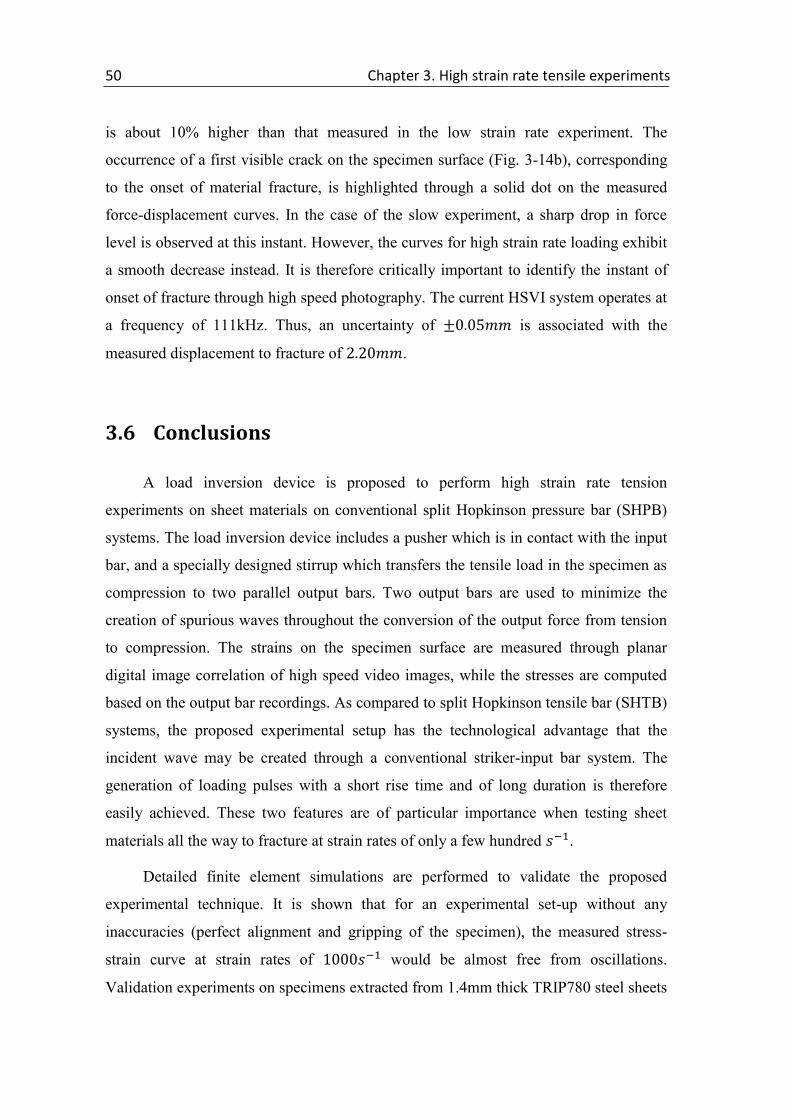
50 Chapter 3. High strain rate tensile experiments
is about 10% higher than that measured in the low strain rate experiment. The
occurrence of a first visible crack on the specimen surface (Fig. 3-14b), corresponding
to the onset of material fracture, is highlighted through a solid dot on the measured
force-displacement curves. In the case of the slow experiment, a sharp drop in force
level is observed at this instant. However, the curves for high strain rate loading exhibit
a smooth decrease instead. It is therefore critically important to identify the instant of
onset of fracture through high speed photography. The current HSVI system operates at
a frequency of 111kHz. Thus, an uncertainty of is associated with the
measured displacement to fracture of .
3.6 Conclusions
A load inversion device is proposed to perform high strain rate tension
experiments on sheet materials on conventional split Hopkinson pressure bar (SHPB)
systems. The load inversion device includes a pusher which is in contact with the input
bar, and a specially designed stirrup which transfers the tensile load in the specimen as
compression to two parallel output bars. Two output bars are used to minimize the
creation of spurious waves throughout the conversion of the output force from tension
to compression. The strains on the specimen surface are measured through planar
digital image correlation of high speed video images, while the stresses are computed
based on the output bar recordings. As compared to split Hopkinson tensile bar (SHTB)
systems, the proposed experimental setup has the technological advantage that the
incident wave may be created through a conventional striker-input bar system. The
generation of loading pulses with a short rise time and of long duration is therefore
easily achieved. These two features are of particular importance when testing sheet
materials all the way to fracture at strain rates of only a few hundred .
Detailed finite element simulations are performed to validate the proposed
experimental technique. It is shown that for an experimental set-up without any
inaccuracies (perfect alignment and gripping of the specimen), the measured stress-
strain curve at strain rates of would be almost free from oscillations.
Validation experiments on specimens extracted from 1.4mm thick TRIP780 steel sheets

3.6. Conclusions 51
are also performed which confirm this result in an approximate manner. In addition,
experiments are performed on notched tensile specimens to demonstrate the capability
of the proposed experimental technique for studying the onset of fracture at high strain
rates.


Chapter 4
Hybrid experimental-numerical
characterization of
the effect of strain rate on fracture
Contents
4.1 Introduction .................................................................................................... 54
4.2 Experimental program ................................................................................... 58 4.2.1 Tensile experiments at low and intermediate strain rate...................... 58
4.2.2 Tensile experiments at high strain rate ................................................ 58 4.2.3 Local displacements and strain measurements .................................... 60
4.3 Experimental results ...................................................................................... 61 4.3.1 Uniaxial tension .................................................................................... 61
4.3.2 Notched tension .................................................................................... 63
4.4 Rate- and temperature-dependent plasticity modeling .................................. 66 4.4.1 Constitutive equations .......................................................................... 66
4.4.2 Model specialization ............................................................................. 68 4.4.3 Calibration procedure .......................................................................... 72
4.5 Numerical analysis and plasticity model validation ...................................... 76 4.5.1 Finite element model ............................................................................. 76 4.5.2 Comparison of numerical and experimental results ............................. 79
4.6 Loading histories to fracture .......................................................................... 80
4.7 Conclusion ..................................................................................................... 86
Abstract
Tensile experiments are carried out on a TRIP780 steel sheet at low ( ),
intermediate ( ) and high strain rates ( ). The experimental program
6 This Chapter is reproduced from: Dunand & Mohr, “Rate-dependent behavior of Advanced
High Strength Steels under multi-axial loading: characterization and modeling at large strains”, submitted
for publication.

54 Chapter 4. Hybrid experimental-numerical characterization of the effect of strain rate on fracture
includes notched as well as uniaxial tension specimens. Local displacements and
surface strain fields are measured optically in all experiments using Digital Image
Correlation. Constitutive equations derived from the Mechanical Threshold Stress
theory are proposed to describe the rate-dependent behavior as well as plastic
anisotropy of the sheet material. Detailed Finite Element simulations of all experiments
reveal that the model accurately predicts experimental results, including force
displacement curves and local surface strain evolution. In particular, the behavior at
large strain, beyond the onset of necking, is well predicted. Stress and strain histories
where fracture initiates are also obtained from the simulations in order to characterize
the dependence of the material ductility to both strain rate and stress state. If the
fracture strain is higher at high strain rate in all experiments, results show that the effect
of strain rate on ductility cannot be considered independently from the state of stress.
4.1 Introduction
The plastic deformation behavior of AHSS steels under uniaxial tension has been
extensively studied during the last decade, indicating that this class of material
experiences positive strain rate sensitivity (e.g. Khan et al., 2012, [91]). Experiments in
the intermediate range of strain rates (1 - 10s-1
) are typically carried out in servo-
hydraulic testing machines (e.g. Huh et al., 2008, [82]) while high strain rate
experiments (100 – 1,000s-1
) are usually performed in Split Hokinson bar systems (e.g.
Van Slycken et al., 2007, [182]; Dunand et al., 2013, [47]) or direct impact setups (e.g.
He et al., 2012, [76]). A key advantage of uniaxial tension experiments is that they give
a direct access to the material response at small strain levels, and especially to the
dependence of flow stress to strain rate. Indeed, force and local displacement
measurements are straightforwardly related to the stress and strain within the range of
uniform elongation. Used in conjunction with optical strain measurement methods, it
also permits to evaluate the effect of strain rate on plastic anisotropy of AHSS sheets
(e.g. Huh et al., 2013, [83]). With the exception of a few experimental results reported
for shear loading conditions (e.g. Rusinek & Klepaczko., 2001, [155]; Peirs et al., 2011,
[147]), virtually no data can be found in the literature describing the multi-axial
behavior of AHSS sheets at high rates of strain.

4.1. Introduction 55
The effect of strain rate on the ductility of AHSS has comparatively been less
evaluated. Most experimental investigations are limited to characterizing uniaxial
tension parameters such as the ultimate elongation (e.g. Olivier et al., 2007, [141]; Huh
et al, 2008, [82]), thereby putting aside the effect of stress state on ductile fracture.
Results presented do not permit to draw a clear trend in the dependence of ultimate
elongation to strain rate for AHSS steels. Kim et al. (2013, [94]) measured increasing
ultimate elongations for increasing strain rates (ranging from 0.1s-1
to 200s-1
) in case of
a DP780 and a TRIP780 steel. Similarly an elongation twice higher at 1000s-1
than at
0.001s-1
is found for a TRIP steel by Verleysen et al. (2011, [185]). On the other hand,
Wei et al. (2007, [189]) report decreasing ultimate elongations with increasing strain
rates in case of two different TRIP-aided steels, while Curtze et al. (2009, [40]) find
almost the same elongation at 10-3
s-1
and 750s-1
for both DP600 and TRIP700 steels. It
is emphasized that the ultimate elongation in a uniaxial tension experiment is a
structural characteristic and not an intrinsic material property. It depends strongly on
the specimen geometry (Verleysen et al., 2008, [184]; Sun et al., 2012, [168]) and is
thus a questionable indicator of material ductility. A somewhat more reliable evaluation
of the fracture strain in uniaxial tension experiments may be obtained by measuring the
reduction of the cross-section area on fractured specimens and assuming a uniform
strain distribution through the sheet thickness. Based on this Reduction of Area
method, Kim et al. (2013, [94]) report a decreasing fracture strain for increasing strain
rates in case of a TRIP780 steel, and a non-monotonic dependence of ductility to strain
rate for DP780 steel.
In most fracture experiments on sheet materials, however, the localization of plastic
deformation through necking cannot be avoided and represents a major difficulty in the
accurate characterization of the material state at fracture. After necking, the stress and
strain fields within the specimen gage section become non-uniform and of three-
dimensional nature (stresses in the thickness direction develop). Consequently, the
stress history prior to fracture can no longer be estimated from the force history
measurements using simple analytical formulas: stress and strain histories prior to
fracture need to be determined in a hybrid experimental-numerical approach (Dunand
& Mohr, 2010, [48]). In other words, a detailed finite element analysis of the
experiment is required to identify the stress and strain fields up to the onset of fracture.

56 Chapter 4. Hybrid experimental-numerical characterization of the effect of strain rate on fracture
The plasticity model used in the numerical simulation is one of the key elements
controlling the accuracy of the method.
An extremely wide variety of constitutive equations describing the rate- and
temperature-dependent plastic behavior of metals have been proposed. The goal of
constitutive equations is to relate the flow stress to strain, strain rate and temperature
(and possibly other internal variables) in order to describe the basic mechanisms of
strain hardening, strain rate sensitivity and thermal softening (and possibly damage,
phase transformation, texture evolution…). Rate-dependent plasticity models can be
categorized into two main branches. On the one hand phenomenological models are
based on the separation of the effects of strain, strain rate and temperature (e.g. Johnson
and Cook, 1983, [88]; Cowper and Symonds, 1952, [39]). Strain hardening, strain rate
sensitivity and thermal softening mechanisms are described by means of basic
functions, depending respectively on strain, strain rate and temperature only, which
may be arbitrarily combined in additive or multiplicative manners to build an ad-hoc
model. A partial review of phenomenological basic functions can be found in Sung et
al. (2010, [169]). Integrated phenomenological models in which variables are not
separated have also been proposed. They allow for description of more complex
mechanisms: temperature-dependent strain hardening (e.g. Sung et al., 2010, [169]),
rate-dependent strain hardening (e.g. Khan et al., 2004, [93])… On the other hand,
attempts have been made to incorporate a description of the mechanisms of plasticity
into physics-based constitutive models (e.g. Zerilli and Armstrong, 1987, [195];
Follansbee and Kocks, 1988, [58]; Voyiadjis and Abed, 2005, [187]; Rusinek et al.,
2007, [157]). Most physics-based models make use of the theory of thermally activated
plastic deformation to relate flow stress, strain rate and temperature (Conrad, 1964,
[38]; Kocks et al., 1975, [95]). Additional internal variables can also be introduced in
the constitutive equations to account for history effects (Bodner and Partom, 1975,
[20]; Durrenberger et al., 2008, [52]). Comparisons between phenomenological and
physics-based models against experimental data tend to show that the latter offer better
predictive capabilities when a wide range of strain rates and/or temperatures is
considered (Liang and Khan, 1999, [111]; Abed and Makarem, 2012, [2]; Kajberg and
Sundin, 2013, [90]).

4.1. Introduction 57
When dealing with sheet materials, plasticity model calibration is usually done
based on uniaxial tension experiments in the range of uniform elongation, as
experimental measurements give direct access to stress, strain and strain rate. The
material behavior at large strains (beyond uniform elongation) is then assumed by
extrapolating the strain hardening at low strains with analytical functions (e.g.
Hollomon, 1945, [79]; Swift, 1952, [170]; Voce, 1948, [186]…). This extrapolation
may lead to inaccurate predictions of the material behavior at large strains. Sung et al.
(2010, [169]) calibrated six different hardening functions for a DP780 based on the
uniaxial data in the range of uniform elongation. Even though all models fit the data
correctly, significant differences are reported at large strains: most extrapolated models
did not represent accurately the material behavior beyond uniform elongation.
In this chapter, tensile experiments are carried out at low, intermediate and high
strain rates to characterize the rate-dependent behavior of a TRIP780 steel. In addition
to uniaxial tension specimens, the experimental program includes tensile specimens
with circular notches. Experiments at high strain rates are performed in the Split
Hopkinson Pressure Bar system described in Chapter 3. Constitutive equations adapted
from the Mechanical Threshold Stress model (Follansbee and Kocks, 1988, [58]) are
proposed to model the dependence of the material behavior to strain rate, as well as
plastic anisotropy. After calibration using an inverse method, the predictive capabilities
of the model are assessed over multiple strain rates and stress states through detailed
Finite Element Simulations of all the experiments. A very good agreement is found
between numerical and experimental results. In particular, accurate predictions of the
post-necking behavior of the sheet material are obtained. A hybrid experimental-
numerical approach is taken to characterize the dependence of ductility to strain rate
and stress state. It is found that the TRIP material exhibits a higher ductility at high
strain rates. However the evolution of ductility between low and intermediate strain
rates depends on the stress state.

58 Chapter 4. Hybrid experimental-numerical characterization of the effect of strain rate on fracture
4.2 Experimental program
4.2.1 Tensile experiments at low and intermediate strain rate
Tensile experiments are performed on straight specimens (Fig. 4-1a) and on flat
specimens with circular cutouts (Fig. 4-1c and 4-1d). The specimen loading axis is
always oriented along the rolling direction. All specimens are extracted from the sheet
material using waterjet cutting. Notched specimens are 20mm wide and feature a
b=10mm wide notched gage section. Specimens with two different notched radii are
prepared: R=20mm and R=6.65mm. Experiments are carried out in a servo-hydraulic
testing machine under displacement control, specimens being hold by friction in
custom-made high pressure clamps. The force applied to the specimen is measured by a
MTS 250kN static load cell, while displacements and strains in the gage section are
measured by Digital Image correlation, as detailed in Section 4.2.4. Two ranges of
strain rates are investigated. For low strain rates, a constant crosshead velocity of
0.84mm/min is imposed to the straight specimens, while a velocity of 0.5mm/min is
chosen for notched specimens. To reach intermediate strain rates, velocities of 22mm/s
and 8.3mm/s are selected for the straight and notched specimens, respectively. All
experiments are carried out at room temperature. Note that the static load cell used is
not correctly dimensioned for intermediate strain rate experiments, leading to
noticeable oscillations in the force measurements (about 1.2% of the measured signal in
amplitude) as visible in Figs. 4-2 to 4-4.
4.2.2 Tensile experiments at high strain rate
The modified Split Hopkinson Pressure Bar system (SHPB) presented in chapter 3
is used to performed high strain rate tensile experiments. In all experiments presented
here, the compressive stress pulse has a total duration of 550µs and a rise time of about
30µs, its magnitude being controlled by the striker velocity. A specifically designed
load-inversion device is used to transform the compressive loading pulse into tensile
loading of the specimen gage section. During deformation of the specimen, the load is
transmitted through the load-inversion device as a compressive stress wave into the

4.2. Experimental program 59
(a) (b)
(c) (d)
Figure 4-1: Uniaxial tension specimens for (a) low and intermediate strain rate and (b)
high strain rate experiments, tensile specimens with a notched radius of (c) 6.65mm
and (d) 20mm. Red dots depict the location of the reference points used to measure
displacements.

60 Chapter 4. Hybrid experimental-numerical characterization of the effect of strain rate on fracture
output bars. The specimen is hold by friction in the load-inversion device, the gripping
pressure being applied by 8 M5 screws. The force applied to the specimen gage section
is derived from elastic waves propagating in the output bars (Eqn. 3-6), while
displacements and strains in the specimen gage section are measured by means of high
speed imaging and digital image correlation. The reader is referred to Chapter 3 for
more details on the experimental set-up and testing procedure.
High strain rate experiments are performed on uniaxial tension specimens, as well
as notched tensile specimens with notch radii of R=20mm and R=6.65mm. Note that
the geometry of the uniaxial specimen, sketched in Fig. 4-1b, is different from the one
used at low and intermediate strain rates. The gage section is shorter (l=15mm instead
of 20mm) and narrower (w=5mm instead of 10mm). On the other hand, the gage
section geometry of the notched tensile specimens is the same at low and high strain
rate. A series of experiments are performed on the three geometries at room
temperature with striker velocities of ranging from 4m/s to 14m/s.
4.2.3 Local displacements and strain measurements
In all tensile experiments, pictures of the specimen surface are recorded to perform
optical-based displacement and strain measurements. For that purpose a thin layer of
white matt paint is applied to the specimen surface along with a black speckle pattern
of a speckle size of about 70μm.
In low strain rate experiments, an AVT Pike F505B with 90mm macro lenses takes
about 300 pictures (resolution of 2048x1024 pixels) before the onset of fracture. The
camera is placed at 1.5m from the specimen surface, resulting in a square pixel edge
length of 23μm. In intermediate and high strain rate experiments, a high speed video
system (Phantom v7.3 with 90mm macro lenses) is used. For intermediate strain rate
experiments, it operates at a frequency of 1kHz with an exposure time of 50μs. A
resolution of 800x600 pixels is chosen. The camera is positioned at a distance of about
400mm from the specimen surface (square pixel edge length of 55μm). In high strain
rate experiments the acquisition frequency is set to 100kHz with a exposure time of
2μs, limiting the spacial resolution to 560x32 pixels. The camera is positioned at a

4.3. Experimental results 61
distance of about 550mm from the specimen surface (square pixel edge length of
70μm).
The virtual extensometer function of the digital image correlation software VIC2D
(Correlated Solutions, SC) is used to determine the relative displacement of two
reference points located on the axis of symmetry of the specimen gage sections. For
this, a quadratic transformation of a 23x23 pixel neighborhood of each point is
assumed. Spline-cubic interpolation of the grey values is used to achieve sub-pixel
accuracy. The position of the DIC reference points on the specimen surface is shown in
Fig. 4-1 with solid red dots. For notched tensile specimens, an initial spacing between
the reference points of is used to compute the relative displacement
imposed to the specimen, while surface strains at the center of the gage sections are
calculated with an initial spacing of . For uniaxial tension, a value of
(resp. ) is chosen at low and intermediate strain rates
(resp. high strain rate). Based on the relative displacement of the two reference
points, the engineering axial surface strain is computed as
(4-1)
4.3 Experimental results
4.3.1 Uniaxial tension
Figure 4-2 depicts the engineering stress-strain curves measured under uniaxial
tension in the three ranges of strain rates. The instant of fracture is indicated with a
solid dot. For low and intermediate strain rates (in black and red in Fig. 4-2,
respectively) the onset of fracture corresponds to a sudden drop of the specimen load
carrying capacity. In the high strain rate experiment, however, the force level decreases
smoothly to zero. The instant of the onset of fracture is therefore identified from the
DIC pictures as the instant at which a first crack appears on the specimen surface. In all
three experiments, a maximum of force corresponding to the onset of localization of the
plastic flow (i.e. necking) is observed. Note that the necking strain decreases as strain

62 Chapter 4. Hybrid experimental-numerical characterization of the effect of strain rate on fracture
Figure 4-2: Experimental engineering stress-strain curves under uniaxial tension.
Results for low strain rates are shown in black, intermediate strain rates in red and
high strain rates in blue. Solid dots correspond to the onset of fracture.
rate increases. Necking occurs at an engineering strain of about 0.2 at low strain rate
(black curve in Fig. 4-2) while it is only 0.14 at high strain rate (blue curve in Fig. 4-2).
For each experiment, a pre-necking strain rate is defined as the time-average of the
axial plastic strain rate (measured by DIC) between initial yielding and the onset of
necking. A pre-necking strain rate of is measured for the experiment at
low strain rate (black curve in Fig. 4-2), for intermediate strain rate
(red curve in Fig. 4-2) and for high strain rate (blue curve in Fig. 4-2).
Note that after the onset of necking, stress and strain fields are no longer uniform in the
specimen gage section. Therefore engineering stress and strains should be interpreted as
normalized forces and displacements, which are structure-level measurements, rather
that local stress and strain measures.
The plastic behavior of the sheet exhibits a weak dependency to strain rate. Both
the initial yield stress and strain hardening are rate-sensitive. The material has the same
initial yield stress but a higher hardening modulus at intermediate strain rate than at low
strain rate. In addition it has a higher initial yield stress but approximately the same

4.3. Experimental results 63
initial hardening modulus at high strain rate than at low strain rate. Before necking, the
stress level is about 100MPa higher in the high strain rate experiment than at low strain
rate. Note that a comparison of the post-necking part of the curves is not meaningful as
different specimen geometries have been used.
4.3.2 Notched tension
Experimental results for the tensile specimen with 20mm notch radii and 6.65mm
notch radii are presented in Fig. 4-3 and Fig. 4-4, respectively. Force displacement
curves for the three strain rates are depicted in Figs. 4-3a and 4-4a, while the evolution
of the engineering axial surface strain at the center of the gage section are plotted in
Figs. 4-3b and 4-4b. The onset of fracture is indicated by a solid dot on all curves. As
for uniaxial tension experiments, it corresponds to a sharp drop of force in low and
intermediate strain rate experiments (in black and red in Figs. 4-3a and 4-4a,
respectively), and to the appearance of the first surface crack in the high strain rate
experiment (in blue in Figs. 4-3a and 4-4a). Note that surface strain measurements are
not available for the high strain rate experiment. Very high strains reached at the center
of the gage section combined with high rates of deformation lead to cracking and
unsticking of the painted pattern used for correlation.
For the 20mm notched specimen, the relative velocities measured between the two
DIC reference points (red points in Fig. 4-1c) are 0.5mm/min for the low strain rate
experiment, 8mm/s for the intermediate strain rate experiment and 7.0m/s for the high
strain rate experiment, respectively. For the 6.65mm notched specimen, the relative
velocities are 0.5mm/min for the low strain rate experiment, 8mm/s for the intermediate
strain rate experiment and 4.5m/s for the high strain rate experiment, respectively. Note
that the reference point locations are the same in all experiments.
Regardless of the geometry or strain rate, all force-displacement curves feature a
maximum of force which corresponds approximately to the onset of localization of the
plastic flow in-plane and through the thickness of the sheet (Dunand & Mohr, 2010,
[48]). Because of the notched geometry, necking always occurs at the center of the gage
section. After the onset of necking, the specimen experiences a loss of load carrying
capacity until fracture occurs. With the 20mm notched specimen (Fig. 4-3a), the loss of

64 Chapter 4. Hybrid experimental-numerical characterization of the effect of strain rate on fracture
(a)
(b)
Figure 4-3: Experimental results of notched tensile specimens with a 20mm radius. (a)
Force displacement curves and (b) Evolution of engineering axial surface strain at the
center of the gage section. Results for low strain rates are shown in black,
intermediate strain rates in red and high strain rates in blue. Solid dots correspond to
the onset of fracture.

4.3. Experimental results 65
(a)
(b)
Figure 4-4: Experimental results of notched tensile specimens with a 6.65mm radius.
(a) Force displacement curves and (b) Evolution of engineering axial surface strain at
the center of the gage section. Results for low strain rates are shown in black,
intermediate strain rates in red and high strain rates in blue. Solid dots correspond to
the onset of fracture.

66 Chapter 4. Hybrid experimental-numerical characterization of the effect of strain rate on fracture
load carrying capacity is about 13% for all strain rates. In case of the 6.65mm geometry
(Fig. 4-4a), however, the force drop before fracture increases with strain rate, from 6%
at low strain rate to 15% at high strain rate. Note that the onset of necking has a non-
monotonic dependence to strain rate. For both geometries, necking occurs at a lower
displacement at intermediate strain rate than at low strain rate, and at a higher
displacement at high strain rate than at intermediate strain rate.
The evolutions of axial surface strain, depicted in Figs. 4-3b and 4-4b for the
20mm and 6.65mm geometries, show a pronounced increase of axial surface strain
rate, which corresponds to localization of the plastic flow. Note that the slope of the
curves plotted in Figs. 4-3b and 4-4b does not correspond, but is proportional to
engineering strain rate as low and intermediate strain rate experiments are run at almost
constant imposed velocity. The change of slope occurring earlier in the intermediate
experiments (in red in Figs. 4-3b and 4-4b) confirms that necking happens at a lower
displacement at intermediate strain rate than at low strain rate. A noticeable difference
between the two geometries concerns the surface strain reached at the onset of fracture
at the center of the gage section. With a notch radius of 20mm (Fig. 4-3b), the surface
axial strain at fracture is lower by 7% at intermediate strain rate ( ) than at low
strain rate ( ), whereas it is higher by 13% at intermediate strain rate ( )
than at low strain rate ( ) with a 6.65mm notch radius (Fig. 4-4b).
4.4 Rate- and temperature-dependent plasticity
modeling
4.4.1 Constitutive equations
A phenomenological approach is taken to model the material behavior. The
material state is described through the Cauchy stress tensor and the absolute
temperature , in conjunction with a set of internal variables: the plastic strain tensor
, the equivalent plastic strain rate and a hardening variable representing the
material resistance to plastic deformation.

4.4. Rate- and temperature-dependent plasticity modeling 67
Incremental plasticity, based on an additive decomposition of the logarithmic strain
tensor is employed
(4-2)
The constitutive equation for stress classically reads
(4-3)
where is the fourth-order isotropic elasticity tensor, characterized by the Young’s
modulus and the Poisson ratio . The effect of thermal expansion is neglected in this
work.
The magnitude of the Cauchy stress is characterized by the equivalent stress
( ) (4-4)
while the flow rule describing the evolution of the plastic strain tensor is defined as
(4-5)
where is a plastic multiplier, and ( ) represents the plastic potential. Note that when
, Eq. 4-5 corresponds to an associated flow rule, while non-associated flow is
modeled otherwise.
The equivalent plastic strain rate is defined as the work-conjugate to the
equivalent stress
(4-6)
where is the rate of plastic work. Upon evaluation of this relationship for the plastic
flow defined in Eq. 4-5, we obtain the following relationship between the equivalent
plastic strain rate and the plastic multiplier
(4-7)
The choice of an associated flow rule yields .

68 Chapter 4. Hybrid experimental-numerical characterization of the effect of strain rate on fracture
The rate and temperature sensitivity of the material behavior is introduced through
the relationship
( ) (4-8)
Finally the material hardening during straining is described by the evolution
equation
( ) (4-9)
Since this work focuses on monotonic loadings only, kinematic hardening is not
considered.
In high strain rate deformation processes, the material is submitted to a temperature
increase due to quasi-adiabatic heating. For the adiabatic case, the temperature rises
according to
(4-10)
Where is the density, the specific heat and the ratio of plastic work
converted to heat. Typically a value of is used (Rusinek and Klepaczko, 2009,
[156]).
4.4.2 Model specialization
The constitutive model defined in Section 4.4.1 is fully characterized by the four
functions ( ), ( ), ( ) and ( ). Specific forms permitting to model
accurately the plastic behavior of the TRIP material are given thereafter.
4.4.2.1 Equivalent stress and flow potential
For the present sheet material, nearly the same stress-strain curve is measured in
uniaxial tension for different specimen orientations even though the Lankford
coefficients are direction dependent. As detailed in Mohr et al. (2010, [122]), we
therefore make use of planar isotropic quadratic yield function, along with a non-
associated flow rule based on a quadratic anisotropic flow potential.

4.4. Rate- and temperature-dependent plasticity modeling 69
√( ) (4-11)
and
√( ) (4-12)
F and G are symmetric positive-semidefinite matrices, with and if and
only if is a hydrostatic stress state. denotes the Cauchy stress vector in material
coordinates,
[ ] (4-13)
The components , and represent the true normal stress in the rolling,
transverse and out-of-plane directions; denotes the corresponding in-plane shear
stress, while and represent the corresponding out-of-plane shear stresses. Note
that in the specific case of quadratic stress and flow potentials defined by Eq. 4-11 and
4-12, Stoughton (2002, [164]) demonstrated that the non-associated flow rule is
consistent with laws of thermodynamics. As shown in Mohr et al. (2010, [122]), the
matrices F and G have only 3 independent coefficients: and , and
.
4.4.2.2 Strain hardening
A review of existing strain hardening functions and rate sensitivity functions ,
governing and respectively, can be found in Sung et al. (2010, [169]). Here, the
hardening modulus ⁄ is considered as stress- and temperature- independent.
Equation 4-9 can therefore be reduced to
( ) (4-14)
Among the numerous hardening laws present in the literature, a saturation
hardening law is selected as it can account for large hardening capabilities of TRIP
steels at low strains as well as a vanishing hardening at very high strains,

70 Chapter 4. Hybrid experimental-numerical characterization of the effect of strain rate on fracture
( ) (
)
(4-15)
4.4.2.3 Strain rate and temperature sensitivity
A constitutive relation derived from the Mechanical Threshold Stress theory (MTS;
Follansbee and Kocks, 1988, [58]) is chosen to describe the dependence of the
equivalent plastic strain rate to the applied stress , the deformation resistance and
temperature . This physics-inspired plasticity model considers dislocation motion as
the only source of plastic deformation and describes it as a thermally activable process.
The deformation resistance to dislocation motion is conceptually decomposed
into two parts,
(4-16)
where represents the part of resistance due to athermal obstacles (typically long
range obstacles such as grain boundaries or large precipitates) and represents the
part of the resistance due to thermally activable obstacles which can be overcome by
thermal fluctuations (typically short range obstacles such as the Peierls resistance,
forest dislocations or solute atoms). Therefore, a lower stress is required to overcome
the short range resistance at higher temperatures. Introducing an effective “thermal”
stress
(4-17)
then the rate of deformation is described by an Arrhenius expression of the form
(Conrad, 1964, [38])
( ) {
{ ( )
}
(4-18)
where is a material constant, the Boltzmann’s constant and is the Gibbs’ free
energy required to overcome the obstacles to dislocation motion with an applied stress,
which is phenomenologically modeled as (Kocks et al., 1975, [95])

4.4. Rate- and temperature-dependent plasticity modeling 71
Figure 4-5: Dependence of flow stress to temperature for low strain rate (in black),
intermediate strain rate (in red) and high strain rate (in blue), at fixed deformation
resistance . is the temperature, depending on strain rate, above which there is
enough thermal energy to overcome short range barriers by thermal activation only.
( ) [ ( )
]
(4-19)
is the activation free energy required to overcome the obstacles to dislocation
motion without the aid of an applied stress.
Strain hardening of the material can be described either by an increase of (e.g.
Kothari and Anand, 1998, [98]), of (e.g. Follansbee and Kocks, 1988, [58]) or both
(e.g. Balasubramanian and Anand, 2002, [8]) during plastic loading. Here we assume
that both and increase at the same rate: the ratio ⁄ is kept constant
throughout loading. Therefore, Eq. 4-18 can be rewritten as
( )
( )
(4-20)
where

72 Chapter 4. Hybrid experimental-numerical characterization of the effect of strain rate on fracture
{ [
( )]
}
( ⁄ )
(4-21)
Figure 4-5 depicts the dependence of the flow stress to temperature for different
strain rates. As detailed in Balasubramanian and Anand (2002, [8]), is the critical
temperature above which there is enough thermal energy for the barriers to be
overcome by thermal fluctuation only, without applying stress. Therefore, at a given
equivalent plastic strain rate , the temperature ( ) is the limit of applicability of
this plasticity model.
4.4.3 Calibration procedure
The rate- and temperature- dependent constitutive model defined in Sections
4.4.1 and 4.4.2 features 17 independent material parameters overall: 2 elastic
coefficients, 3 coefficients defining the equivalent stress function (Eq. 4-11), 3
coefficients defining the plastic flow potential (Eq. 4-12), 4 coefficients defining the
strain hardening function (Eq. 4-15) and 5 coefficients defining the rate sensitivity
function (Eq. 4-18). The calibration procedure is given thereafter. The set of
parameters calibrated for the present TRIP material are given in Table 4-1.
The equivalent stress function and plastic flow potential are calibrated based
on uniaxial tension experiments carried out at low strain rate. Corresponding matrices F
and G are calibrated following the procedure described in Mohr et al. (2010, [122]).
Since the spacial resolution of high speed imaging system is not sufficient to measure
the Lankford coefficients in high strain rate tension experiments, it is assumed that the
anisotropy of the plastic flow observed at low strain rate is independent from the strain
rate. The flow potential is therefore assumed rate-independent. Note that because of a
lack of experimental data characterizing the out-of-plane behavior of the sheet material,
coefficients of F and G corresponding to out-of-plane shear are set equal to 3 (isotropic
value).
An optimization based inverse method is carried out to calibrate the coefficients
of the strain hardening and rate sensitivity functions. The objective of the optimization

4.4. Rate- and temperature-dependent plasticity modeling 73
Table 4-1: Material parameters for the rate-dependent model
Elastic constants Strain hardening parameters
[MPa] [-] [MPa] [MPa] [MPa] [-]
185,000 0.3 503 1,383 41,505 2.513
Strain rate sensitivity parameters
[s-1
] [J] [-] [-] [-]
67,457 8.794E-20 1.911 1.861 0.1949
Equivalent stress and flow potential parameters
[-] [-] [-] [-] [-] [-] [-]
1 1 1.076 2.925 -0.462 -0.538 -0.538
[-] [-] [-] [-] [-] [-] [-]
1 0.873 1.071 3.13 -0.401 -0.599 -0.472
process is to find the set of parameters that leads to the best prediction of the force-
displacements curves of the notched tensile specimen with a 6.65mm radius measured
in low, intermediate and high strain rate experiments. For a given set of parameters ,
numerical simulations of the 6.65mm notched tensile specimen are carried out for the
three different strain rates, using the Finite Element model described in Section 4.5.1.
Then the three predicted force-displacement curves are compared to experimental
measurements up to the fracture displacement to evaluate the cost function for the
set of parameters
( ) ∑{
∫ ( )[ ( ) ( )]
}
(4-22)
where is the number of calibration tests and is a weighting factor used to focus
the fitting process on the part of the force-displacement curves located between
maximum force and the onset of facture. Before maximum force is reached ,

74 Chapter 4. Hybrid experimental-numerical characterization of the effect of strain rate on fracture
(a)
(b)

4.4. Rate- and temperature-dependent plasticity modeling 75
(c)
Figure 4-6: Experimental (points) and simulation (solid curves) results for the notched
tensile specimen with a radius, at (a) low, (b) intermediate and (c) high
strain rate. Force displacement curves are in black and engineering axial strain versus
displacement curves in blue. The dashed lines depict the instant of fracture.
while beyond maximum force. A downhill simplex minimization algorithm
(Nelder and Mead, 1965, [133]) is used to find the set of parameters that
minimizes , as it requires the evaluation of the error function only, but not its
derivatives
( ) (4-23)
Overall 640 iterations were required to converge to a minimum. Corresponding
force displacement curves are shown in Fig. 4-6. Numerical predictions (solid black
lines in Fig. 4-6) are in very close agreement with experimental results (black dots in
Fig. 4-6) for all three strain rates, including after the maximum of force is reached.
Note that the resulting set of optimal parameters, given in Table 4-1, corresponds only
to a local minimum of the error function . This optimal set might not be the unique set
of parameters minimizing , and it is not necessarily the best possible set (absolute
minimum of ).

76 Chapter 4. Hybrid experimental-numerical characterization of the effect of strain rate on fracture
4.5 Numerical analysis and plasticity model validation
4.5.1 Finite element model
Dynamic explicit simulations of each tensile experiment are carried out using the
commercial Finite Element Analysis package Abaqus (2011, [1]). The constitutive
model described in Section 4.4 is implemented as a user material through the VUMAT
interface (see Appendix A for details on the implementation). Specimens are meshed
with reduced integration brick elements with a temperature degree of freedom (type
C3D8RT of the Abaqus library). Exploiting the symmetry of the notched specimen
geometries, material properties and loading conditions, only one eighth of the notched
specimens are modeled: the mesh represents the upper right quarter of the tensile
specimens, with half the thickness. The distance between the center of the gage section
and the upper mesh boundary corresponds exactly to half the length of the virtual
extensometer used to measure displacements during the experiments. Note that
experimental observations demonstrate that plastic localization also respects the
specimen symmetries. Reduced meshes can therefore be used to model the post-
necking behavior of notched tensile specimens. In uniaxial tension experiments,
however, so-called diffuse necking leads to a slanted band of plastic localization that
does not respect the initial symmetries. The meshes used for uniaxial tension model the
full specimen geometries, including the specimen shoulders.
In all tensile experiments carried out, the plastic flow localizes before the onset of
fracture, leading to steep gradients of stresses and strains both in-plane and through the
sheet thickness. To capture accurately the post-necking behavior, a fine mesh featuring
8 elements through the half-thickness and an element in-plane dimension of 0.1mm at
the center of the gage section is used (see Chapter 5 for details).
Simulations of each loading condition are performed. For that purpose half the
experimental velocity measured by DIC is uniformly imposed to the upper boundary of
the mesh. A zero normal displacement condition is imposed to boundaries
corresponding to symmetry planes. Simulations are run slightly beyond the
displacement at which fracture occurs in the experiment. To speed up calculations,
uniform mass scaling is used in the low strain rate simulations. The material density is

4.5. Numerical analysis and plasticity model validation 77
artificially adjusted to reach the fracture displacement within 300,000 time increments.
High strain rate experiments are simulated with the real material density (7.8g/cm3),
resulting in an initial stable time increment of 1.1x10⁻⁸
s and about 50,000 increments.
To account for both temperature increase due to plastic work and heat diffusion
due to temperature gradients, the “temperature-displacement analysis” capability of the
Abaqus/Explicit solver is used to simulate the intermediate and high strain rate
experiments. In this type of Finite Element analysis, both the equilibrium and heat
transfer equations are solved. Since most plastic deformation and thus most heat
generation are localized at the center of the gage section, no heat flow is modeled on
the upper boundary of the mesh. In addition, a no heat flow condition is also imposed
to the boundaries corresponding to symmetry planes. Furthermore, no heat transfer is
considered at the specimen surface. A material specific heat of 490 J/K/kg and a
conductivity of 45 J/s/m/K are chosen. Low strain rate experiments are modeled as
isothermal.
Figure 4-7: Experimental (points) and simulation (solid curves) results for uniaxial
tension at low (black curve), intermediate (red curve) and high strain rate (blue curve).
The dashed lines depict the instant of fracture.

78 Chapter 4. Hybrid experimental-numerical characterization of the effect of strain rate on fracture
(a)
(b)

4.5. Numerical analysis and plasticity model validation 79
(c)
Figure 4-8: Experimental (points) and simulation (solid curves) results for the notched
tensile specimen with a radius, at (a) low, (b) intermediate and (c) high
strain rate. Force displacement curves are in black and central logarithmic axial strain
versus displacement curves in blue. The dashed lines depict the instant of fracture.
4.5.2 Comparison of numerical and experimental results
Figures 4-6 to 4-8 present a comparison between results from numerical
simulations (solid lines) of all tensile experiments and experimental measurements
(solid dots). The instant of the onset of fracture is depicted for all experiments through
a vertical dashed line. Recall that only the force-displacement curves of the 6.65mm
notched tensile experiments (in black in Fig. 4-6) are used to calibrate the proposed
plasticity model. All other results may be seen as model validation.
Uniaxial engineering stress strain curves are shown in Fig. 4-7. The numerical
engineering strain is computed according to Eq. 4-1 from the displacements of nodes
positioned at the same location as DIC reference points, while the numerical
engineering stress is obtained from the force applied at the specimen boundaries
normalized by the gage section initial cross section area. Experimental results at both
intermediate (in red in Fig. 4-7) and high strain rate (in blue in Fig. 4-7) are extremely

80 Chapter 4. Hybrid experimental-numerical characterization of the effect of strain rate on fracture
well predicted, as numerical results (solid lines) and experimental measurements (solid
dots) lie almost exactly on top of each other up to fracture. Note that the loss of load
carrying capacity preceding fracture is correctly predicted in both cases. Concerning the
low strain rate experiment (in black in Fig. 4-7), the stress strain curve is well predicted
in the range of uniform elongation (before maximum engineering stress is reached).
However, the force level is underestimated after the onset of necking, resulting in a
predicted force 7% lower than the experimental one at the onset of fracture.
In Fig. 4-8, we show the simulated force-displacement curves (solid black lines) of
the 20mm notch geometry for low (Fig. 4-8a), intermediate (Fig. 4-8b) and high (Fig.
4-8c) strain rates. The agreement with experimental results is very good all the way to
the onset of fracture. The relative difference between experimental and predicted forces
does not exceed 3%.
The comparison of the evolution of the surface axial strain at the center of the
gage section of notched specimens with respect to the displacement (depicted in blue in
Figs. 4-6 and 4-8) also shows a good agreement. Irrespective of the notch radius and
the strain rate, the simulations are able to describe the characteristic increases in strain
rates that have been observed in the experiments. Relative differences between
simulation and DIC strains in case of the 6.65mm notch geometry are about 5% at low
strain rate (Fig. 4-6a) and 6% at intermediate strain rate (Fig. 4-6b) at the onset of
fracture. For the 20mm notch geometry (Fig. 4-8), the computed strain almost exactly
corresponds to the DIC strain, with less than 1% relative error for both strain rates.
4.6 Loading histories to fracture
Stress and strain fields are heterogeneous both in-plane and through the thickness
in all experiments performed, because of specimen geometries and plastic flow
localization through necking. It is therefore not possible to obtain an accurate estimate
of the evolution of stress, strain and strain rate up to fracture from either global (force-
displacement curve) or local (surface strains from DIC) experimental measurements
(Dunand and Mohr, 2010, [48]). Instead the evolutions of stress state, strain and strain
rate are obtained from the Finite Element simulations presented in Section 4.5. From

4.6. Loading histories to fracture 81
each simulation, the loading histories are extracted from the integration point where the
equivalent plastic strain is highest at the onset of fracture, which is thereby assumed to
be the location where fracture initiates. Recall that the onset of fracture is considered to
be reached in the simulation when the imposed displacement corresponds to the
experimentally measured displacement at which a first crack appears at the specimen
surface.
Figures 4-9 to 4-11 summarize the loading histories to fracture in all experiments.
The evolutions of strain rate and stress state are shown in Figs. 4-9 and 4-10,
respectively. Figure 4-11 depicts the evolution of the equivalent plastic strain versus
stress state for all geometries and loading conditions.
The plastic localization associated with necking has a profound influence on the
local material state. Despite constant velocities applied to the specimen boundaries, the
local strain rate dramatically increases after the onset of necking. In the 20mm notch
specimens, the equivalent plastic strain rate is 20 times larger at the onset of fracture
than before the onset of necking. In the low strain rate experiment, the strain rate
increases from 5x10⁻⁴
s-1
to 10-2
s-1
(black line in Fig. 4-9b). The increase ranges from
0.53s-1
to 10.5s-1
in the intermediate strain rate experiment (in red in Fig. 4-9b) and
from 500s-1
to 10.2x10³s
-1 in the high strain rate experiment (in blue in Fig. 4-9b).
Similar increases of strain rates are observed in the 6.65 notch experiment (Fig. 4-9c).
In uniaxial tension experiments (Fig. 4-9a), the increase of strain rate due to necking is
even more pronounced. In the low strain rate loading (in black in Fig. 4-9a), the
equivalent plastic strain rate is 40 times larger at the onset of fracture ( =3.2x10⁻²
s-1
)
than before necking ( =8x10⁻⁴
s-1
).
Figure 4-10 depicts the stress state trajectory in the ( ) space for the three low
strain rate experiments, while the loading trajectories in the ( ) space and the
( ) space are shown for all experiments in Fig. 4-11a and 4-11b respectively. Solid
points in Figs. 4-10 and 4-11 mark the onset of fracture. Even though experiments are
performed on a sheet material, the stress states at fracture (solid dots in Fig. 4-10)
significantly differ from the plane stress condition (represented by a dashed line in Fig.
4-10). After the onset of necking, the triaxiality increases (Fig. 4-11a) and the third
invariant decreases (Fig. 4-11b) continuously in all experiments. In the specific case of

82 Chapter 4. Hybrid experimental-numerical characterization of the effect of strain rate on fracture
(a)
(b)

4.6. Loading histories to fracture 83
(c)
Figure 4-9: Numerical prediction of the evolution of equivalent plastic strain rate versus
equivalent plastic strain at the location where fracture is assumed to initiate in (a)
uniaxial tension, (b) 20mm notch tension and (c) 6.65mm notched tension
experiments. Solid dots indicate the onset of fracture.
uniaxial tension at high strain rate, the triaxiality ramps up from to
while the third invariant decreases from down to .
The equivalent plastic strain reached at the onset of fracture, or fracture strain ,
strongly depends on both the stress state and the strain rate. In a given range of strain
rate, the fracture strain monotonically decreases when moving from uniaxial tension to
TPS tension. At low strain rate (black curves in Fig. 4-11), the fracture strain is 60%
higher in the 20mm notch specimen ( ) and 118% higher in the uniaxial
specimen ( ) than in the 6.65mm notch specimen ( ). The
dependence of the fracture strain to strain rate appears to be stress state dependent. In
case of the 6.65mm notch specimen, it increases monotonically with strain rate, from
to at intermediate strain rate and at high strain rate. In
the case of 20mm notch tension specimens, however, the dependence is non-
monotonic. The fracture strain at intermediate strain rate ( ) is lower than at

84 Chapter 4. Hybrid experimental-numerical characterization of the effect of strain rate on fracture
Figure 4-10: Loading path in the ( ) plane for low strain rate experiments. Solid dots
indicate the instant of fracture. The black dashed line shows the relation between
stress triaxiality and third stress invariant in case of plane stress condition.
low strain rate ( ) by 7%, but it is highest at high strain rate ( ). The
effect of strain rate is even more pronounced with the uniaxial tension specimen, in
which the fracture strain at intermediate strain rate ( ) is lower than at low
strain rate ( ) by 21%, while it is higher at high strain rate ( ) by
34%.
Note that for a given geometry, the stress state evolution is more or less
independent from the strain rate, as shown in Fig. 4-11. Differences in the fracture
strain for different loading conditions on a given specimen are therefore attributed to
the dependence of the material ductility to strain rate, and not to a variation in the stress
state evolution.

4.6. Loading histories to fracture 85
(a)
(b)
Figure 4-11: Loading paths to fracture at low (black lines), intermediate (red lines) and
high strain rate (blue lines). (a) Evolution of equivalent plastic strain versus stress
triaxiality and (b) evolution of equivalent plastic strain versus normalized third stress
invariant in all experiments. Solid points depict the onset of fracture.

86 Chapter 4. Hybrid experimental-numerical characterization of the effect of strain rate on fracture
4.7 Conclusion
The deformation behavior of TRIP780 steel sheets is investigated for different
stress states over a wide range of strain rates. Tensile experiments have been carried on
notched specimens as well as on uniaxial specimens, using a hydraulic testing machine
(for low and intermediate strain rates) and a Split Hopkinson Pressure Bar system (for
high strain rate loadings). Positive, but rather weak, strain rate sensitivity is observed.
Constitutive equations derived from the MTS theory are proposed to capture the
dependence of the material behavior to strain rate as well as the plastic anisotropy
observed at low strain rate. The model is calibrated with an inverse optimization
method from the force-displacement response of notched tensile specimens deformed at
different strain rates, up to fracture. A comparison between experimental results and
detailed Finite Element simulations of all the experiments show that the constitutive
model can predict accurately the material behavior over all the range of strain rates and
stress states considered. In particular, the material behavior at large strains, after the
onset of localized necking, is well captured.
A hybrid experimental-numerical approach is followed to evaluate the material
loading histories up to the onset of ductile fracture in all experiments. It is shown that
the equivalent strain at the onset of fracture is significantly higher at high strain rate
than at low and intermediate strain rates. However, results reveal that the dependence
of the fracture strain to strain rate is not similar in all types of experiments carried out.
In particular the material ductility is lower at intermediate strain rate than at low strain
rate for stress states close to uniaxial tension, while the opposite is observed for stress
states close to transverse plane strain tension. As a result, the effects of strain rate and
stress state should not be considered separately when developing and calibrating rate-
dependent fracture models for AHSS sheets.

Chapter 5
Numerical methods for accurate and
efficient ductile fracture predictions
Contents
5.1 Introduction .................................................................................................... 88
5.2 An uncoupled fracture model for Advanced High Strength Steel sheets ...... 89
5.2.1 Plasticity model .................................................................................... 89 5.2.2 Fracture model ..................................................................................... 90
5.3 Influence of Finite Element modeling on ductile fracture predictions .......... 91
5.3.1 Methodology ......................................................................................... 93
5.3.2 Results for shell elements ...................................................................... 94 5.3.3 Results for solid elements ..................................................................... 97 5.3.4 Comparison shell-solid ....................................................................... 100
5.3.5 Mixed shell-solid model ...................................................................... 102
5.4 Dynamic shell-to-solid re-meshing .............................................................. 105
5.4.1 Principle ............................................................................................. 105 5.4.2 Simple example ................................................................................... 107 5.4.3 Application to basic fracture experiments .......................................... 110
5.5 Conclusion ................................................................................................... 118
Abstract
The influence of spacial discretization in FE simulations on predictions of
mechanical response and ductile fracture in AHSS structures is analysed. The inability
of shell elements to accurately predict the post-necking behavior of sheet materials is
highligted. On the contrary predictions independent from the mesh characteristics are
obtained with solid elements if sufficiently fine meshes are used. However, intensive
computation efforts associated with the use of fine meshes of solid elements to model
sheet structures such as automootive parts make it unsuitable to an industrial
7 The work described in this chapter has been carried out at E.S.I. group in Rungis, France, as part
of a six month part-time collaboration.

88 Chapter 5. Numerical methods for accurate and efficient ductile fracture predictions
environment. A dynamic shell-to-solid re-meshing technique is considered to benefit
from both the numerical efficiency of shells and the accuracy of fine solid meshes.
Comparisons of numercial predictions using re-meshing to experimental results show a
significant increase of the accuracy of fracture predictions compared to shell
simulations, and substantial time savings compared to solid simulations.
5.1 Introduction
With the generalization of virtual engineering practices in the development and
design of new vehicles, an accurate and predictive modeling of ductile fracture in sheet
materials has become a significant issue. However, in an industrial context, an
appropriate balance must be found between numerical efficiency and accuracy. Finite
element simulations of the mechanical response of sheet structures are therefore
commonly performed with shell elements, which allow for faster computations.
However, fracture predictions using shell elements are often compromised by the
dependence of shell models submitted to large deformation to the mesh size.
This chapter focuses on the influence of the finite element modeling on ductile
fracture predictions in Advanced High Strength Steel sheets. For that purpose the
influence of the type of elements used and their characteristic size is investigated. Finite
element simulations of a flat notched specimen submitted to tension (which is typically
used to characterize experimentally the onset of ductile fracture in sheet materials) are
carried out with both shell and solid elements, with five different mesh densities.
Simulation results are compared in terms of the predicted force displacement curves
and the predicted displacement at which the onset of ductile failure occurs, and the
local stress, strain and damage evolutions are also analyzed. Results show that in the
early stages of the simulation, both shell and solid elements give comparable results,
regardless of the mesh size. However fracture predictions are significantly different,
depending on the mesh size and type. The critical instant after which shell elements
give inaccurate results is the onset of through-the-thickness localization. After the onset
of localized necking, shells are not able to predict the local stress state correctly,
resulting in a spurious localization of the deformation and inaccurate and mesh-size-
dependent fracture predictions. Solid elements, however, are able to predict the material

5.2. An uncoupled fracture model for Advanced High Strength Steel sheets 89
evolution after the onset of necking, and give results independent from the mesh size if
it is small enough. This increased accuracy is obtained at the expense of computational
efficiency.
Consequently, a shell-to-solid re-meshing technique permitting to refine locally
the shell mesh into solid elements during the simulations, in areas where the sheet
material experiences localized necking, is presented. Improved shell simulations using
re-meshing are carried out and evaluated. The accuracy of the re-meshing technique is
evaluated based on numerical simulations of tensile fracture experiments and on a
comparison between numerical predictions and experimental results. It is shown that
the accuracy of shell simulations is increased when using re-meshing. In particular, the
post-necking behavior of the sheet material can be captured correctly. In addition, using
shell-to-solid re-meshing offers about 75% savings on the computational cost compared
to simulations with solid elements.
In this chapter we limit our attention to low strain rate experiments and rate-
independent plasticity and fracture models.
5.2 An uncoupled fracture model for Advanced High
Strength Steel sheets
We make use of a rate-independent simplification of the plasticity model
proposed in Chapter 4. The onset of ductile farcture will be modeled independently
using the so-called Modified Mohr-Coulomb (MMC) model (Bai and Wierzbicki,
2010, [7]). The predictive capabilities of the constitutive and fracture models described
thereafter are not investigated here. The reader is referred to Mohr et al. (2010, [122])
and Dunand and Mohr (2011, [49]) for a critical evaluation.
5.2.1 Plasticity model
For the present sheet material, nearly the same stress-strain curve is measured for
different specimen orientations even though the r-values are direction dependent. As

90 Chapter 5. Numerical methods for accurate and efficient ductile fracture predictions
detailed in Mohr et al. (2010, [122]), we make use of a planar isotropic quadratic yield
function,
( ) √( ) (5-1)
in conjunction with a non-associated flow rule
(5-2)
denotes the plastic multiplier. The anisotropic quadratic flow potential reads
√( ) (5-3)
P and G are symmetric positive-semidefinite matrices, with and if and
only if is a hydrostatic stress state. The values for the non-zero components of P and
G are given in Table 5-1. denotes the Cauchy stress vector in material coordinates,
[ ] (5-4)
The components , and represent the true normal stress in the rolling,
transverse and out-of-plane directions; denotes the corresponding in-plane shear
stress, while and represent the corresponding out-of-plane shear stresses.
Isotropic strain hardening is described as
( ) (5-5)
where ( ) defines the strain hardening modulus. The strain hardening response
of the material is modeled by a saturation law
( ) ( ( )
)
(5-6)
5.2.2 Fracture model
The original Mohr-Coulomb failure criterion (Mohr, 1900, [127]) is formulated in
the stress space and assumes that failure occurs when the shear and normal stresses on
any plane of normal vector n verify the condition

5.3. Influence of Finite Element modeling on ductile fracture predictions 91
( ) (5-7)
with the friction coefficient and the cohesion . Bai and Wierzbicki (2010, [7])
transformed Eq. (5-7) into the space of stress triaxiality, Lode angle and equivalent
plastic strain to fracture assuming proportional monotonic loading, a pressure and Lode
angle dependent isotropic plasticity model, and isotropic strain hardening according to
the power law. The resulting explicit expression for the fracture strain reads
( ) { [ √
√ ( ( ) ) ( (
) )]
[√
(
) (
(
))]}
(5-8)
with
( ) {
(5-9)
The exponent n describes the strain hardening of the material. The coefficient
is related to in Eq. (5-7), while and characterize the dependence of the
underlying plasticity model on the third stress invariant. controls the amount of Lode
angle dependence of the fracture locus and ( ) controls the asymmetry of the
fracture locus with respect to the plane . Despite the discontinuity of ( ), the
fracture strain ( ) is a continuous function of the stress invariants and . To apply
the MMC fracture model for non-proportional loadings, Bai and Wierzbicki (2010, [7])
make use of Eq. (5-8) as reference strain in Eq. (2-19).
5.3 Influence of Finite Element modeling on ductile
fracture predictions
The influence of the type of elements (brick vs shell) and their characteristic
dimensions are investigated on numerical simulations of a tensile experiment on a flat
specimen with circular notches of radius 6.67mm, as sketched in Fig. 4-1c. Parameters
for the constitutive model described in Section 5.2 have been calibrated on an extensive

92 Chapter 5. Numerical methods for accurate and efficient ductile fracture predictions
Table 5-1: Material parameters for the TRIP780 steel
Yield
function
[-] [-] [-] [-] [-] [-] [-]
1.00 1.00 1.06 2.94 -0.47 -0.53 -0.53
Flow
potential
[-] [-] [-] [-] [-] [-] [-]
1.00 0.94 1.00 2.64 -0.47 -0.53 -0.47
Hardening [MPa] [MPa] [MPa] [-]
459 1173 20425 1.867
MMC [-] [-] [-] [-] n [-]
0.3472 0.9098 1.7003 1.546 0.204
(a) (b) (c)
Figure 5-1: Meshes of the notched tensile specimen. (a) very coarse mesh; (b)
medium mesh and (c) very fine mesh.

5.3. Influence of Finite Element modeling on ductile fracture predictions 93
set of multi-axial fracture experiments carried out on TRIP780 steel (Mohr et al., 2010,
[122]; Dunand and Mohr, 2011, [49]). Note that this material comes from a different
production batch than the one used in Chapters 3, 4 and 6. Materials parameters are
thus slightly different.
5.3.1 Methodology
Finite element simulations are run with five different mesh densities, shown in
Fig. 5-1:
(i) very coarse mesh with an element edge length of at the specimen
center and elements in thickness direction (half thickness),
(ii) coarse mesh with and ;
(iii) medium mesh with and ;
(iv) fine mesh with and ;
(v) very fine mesh with and .
Figure 5-2: View of the very fine mesh with 12 solid elements through the half-
thickness

94 Chapter 5. Numerical methods for accurate and efficient ductile fracture predictions
Note that the medium shell mesh corresponds to current standard practices in
industrial simulations of car crash tests. Meshes with both only shell and only solid
elements are considered. For a given density, shell and solid meshes are identical in the
sheet plane. Only the number of elements through the thickness varies (1 for shell,
for solids). Because of the symmetries of the notched specimen, only ⁄ of the
specimen is meshed, and half the thickness for solid meshes. A displacement boundary
condition is imposed to the upper boundary of the specimen (constant velocity). All
simulations are run up to an imposed displacement of 1.5mm. Fracture is assumed to
occur when the critical damage is reached at any integration point in the model.
Note that element deletion is not used in the present simulations.
5.3.2 Results for shell elements
Force displacement curves predicted with the five meshes are depicted in Fig. 5-
3. The instant at which fracture occurs is highlighted by a solid square on each curve.
After the maximum of force is reached (which corresponds to the onset of localization
of the plastic flow through the thickness of the specimen (localized necking)),
simulation results show a very strong dependence to mesh size. More specifically, the
finer the mesh, the more abrupt the force decreases after necking and the smaller the
fracture displacement. It must be noted that simulation results do not converge as the
mesh is refined. For most of the mesh densities, fracture occurs earlier than in the
experiment. With the very fine mesh, fracture occurs in the simulation just after the
maximum of force is reached.
Figure 5-4 compares the evolution of damage (solid line) and equivalent plastic
strain (dashed line) at the center of the specimen for the very fine (in red) and very
coarse mesh (in black). Both simulations give the same results before the maximum of
force (displacement smaller than 0.8mm). But after the maximum of force, the
evolution of damage and plastic strain strongly depends on the mesh size. For the very
fine mesh, damage exhibits a sharp increase after necking, leading to an almost
instantaneous fracture after the maximum of force.
Regardless of the element dimensions, all the deformation localizes in a band of 1
element width at the center of the gage section after the maximum of force is reached,

5.3. Influence of Finite Element modeling on ductile fracture predictions 95
Figure 5-3: Predicted force displacement curves with shell elements. The predicted
instant of fracture is shown by a solid circle for each simulation. The experimental
instant of fracture is depicted by a dashed black line.
Figure 5-4: Evolution of damage and equivalent plastic strain at the center of the
notched specimen, for the very fine (red) and very coarse (black) meshes with shell
elements. The experimental instant of fracture is depicted by a dashed black line.
0
2
4
6
8
10
12
14
16
0 0.5 1 1.5
Forc
e [
kN]
Displacement [mm]
Shell elements
fracture prediction
very coarse
coarse
medium
fine
very fine
0
1
2
3
4
5
6
7
0 0.5 1 1.5
Dam
age
[-]
Equ
ival
ent
pla
stic
str
ain
[-]
Displacement [mm]
damage, verycoarse
damage, veryfine
eq. plast. Strain,very coarse
eq. plast. strain,very fine

96 Chapter 5. Numerical methods for accurate and efficient ductile fracture predictions
Figure 5-5: Contour plot of equivalent plastic strain after the maximum of force , using
a fine mesh of shell elements
as illustrated in Fig. 5-5. This spurious localization leads to very high values of strain
and damage inside that band, so that fracture occurs right after the maximum force
when using fine meshes.
After necking, a three dimensional stress state develops in the material. In
particular, through-the-thickness stresses appear and permit to bring additional strain
hardening capabilities that is needed to compensate sheet thinning. However those
mechanisms cannot be captured by shell elements, in which the state of stress is
necessarily plane stress. As a result, shells cannot predict correctly the material
evolution (stress and strain state) after necking, regardless of the element size. To

5.3. Influence of Finite Element modeling on ductile fracture predictions 97
illustrate this point, Fig. 5-6 depicts the evolution of the stress triaxiality and equivalent
plastic strain at the center of the specimen, when a medium mesh is used. After necking
(at an equivalent plastic strain of about 0.2), the stress triaxiality increases but rapidly
saturates at a value of , which corresponds to transverse plane strain tension: it
is the maximum of triaxiality achievable under plane stress with traction applied in only
one direction. However, in the actual specimen, higher triaxialities are reached, because
of the three dimensional stress state that develops.
Figure 5-6: Evolution of the stress triaxiality and the equivalent plastic strain at the
center of the specimen, as predicted by a fine mesh of shell elements (black line) and
solid elements (red line).
5.3.3 Results for solid elements
Force displacement curves predicted with the five different solid meshes are
depicted in Fig. 5-7. The instant at with fracture occurs is highlighted by a solid square
on each curve. All simulations predict the same force displacement curve before the
maximum of force, but some differences become noticeable thereafter. However, it
should be noted that the medium, fine and very fine mesh predict the same force res-
0
0.1
0.2
0.3
0.4
0.5
0.6
0.7
0.8
0.9
1
0.4 0.5 0.6 0.7 0.8 0.9 1
Eq. p
last
ic s
trai
n [
-]
Stress triaxiality [-]
shell
Solid

98 Chapter 5. Numerical methods for accurate and efficient ductile fracture predictions
Figure 5-7: Predicted force displacement curves with solid elements. The predicted
instant of fracture is shown by a solid circle for each simulation. The experimental
instant of fracture is depicted by a dashed black line.
Figure 5-8: Evolution of the equivalent plastic strain at the center of the gage section
for different mesh densities. The experimental instant of fracture is depicted by a
dashed black line.
0
2
4
6
8
10
12
14
16
0 0.5 1 1.5
Forc
e [
kN]
Displacement [mm]
Solid elements
fracturepredictionvery coarse
coarse
medium
fine
very fine
0
0.2
0.4
0.6
0.8
1
1.2
1.4
1.6
0 0.2 0.4 0.6 0.8 1 1.2 1.4
Eq. p
last
ic s
trai
n[-
]
Displacement [mm]
very coarse
coarse
medium
fine
very fine

5.3. Influence of Finite Element modeling on ductile fracture predictions 99
Figure 5-9: Contour plot of equivalent plastic strain after the onset of localized necking,
with the very fine solid mesh.
ponse up to a displacement of 1mm, while the fracture displacement is 1.03mm: results
converge as the mesh is refined. Similarly, the predicted fracture displacement
decreases as the mesh is refined, but eventually converges: almost the same fracture
displacement is predicted by the fine and very fine mesh.
The evolution of the equivalent plastic strain at the center of the gage section is
depicted for all five mesh densities in Fig. 5-8. As for force-displacement curves, all
curves are identical for displacements lower than 0.8mm, which corresponds to the
maximum of force. After that instant, results become mesh size-dependent: the finer the
higher, the steeper the increase of equivalent plastic strain. However, at least in the
range of displacements lower than the experimental fracture displacement (black
dashed line in Fig. 5-8), results converge as the mesh is refined: for displacements
lower than , the evolution of equivalent plastic strain is the same with the fine and
very fine meshes.
The force displacement curves depicted in Fig. 5-7 exhibit a maximum of force
(for a displacement of about 0.8mm). This maximum corresponds to the onset of
localized necking at the center of the specimen gage section. As shown in Fig. 5-9,
localized necking provokes a severe thickness reduction at the center of the specimen,

100 Chapter 5. Numerical methods for accurate and efficient ductile fracture predictions
and through-the-thickness gradients in the stress and strain fields. In addition, a three
dimensional stress state develops, with significant out-of plane stresses building up.
Solid meshes with more than 1 layer of elements in the thickness direction can
predict the three dimensional stress states that develops in the material after the onset of
localized necking. Figure 5-6 depicts the evolution of equivalent plastic strain and
stress triaxiality at the center of the specimen with a fine solid mesh (in red). The
simulation is able to capture the increase of stress triaxiality after necking due to the
building-up of out-of-plane stresses.
5.3.4 Comparison shell-solid
Before the onset of necking, shell and solid elements give the same results,
regardless of the mesh density. Differences between mesh types and mesh densities
become noticeable – and significant – only after the onset of through-the-thickness
necking.
Figure 5-10 shows the predicted fracture displacement as a function of the mesh
characteristic length. With both shell elements and solid elements, the prediction of
fracture displacement seems to converge with respect to mesh size: the fine and very
fine meshes lead to same results. In case of solid elements, the converged result is very
close to the experimental displacement to fracture. However, in case of shell elements,
the prediction for the fracture displacement converges towards the value of
displacement at which the maximum of force occurs, which means that the accuracy of
fracture predictions using shell elements cannot be increased by “tuning” the material
parameters of the fracture model.
Table 5-2: CPU time (in s) for different mesh types and densities
Very coarse Coarse Medium Fine Very fine
Shell 5.4 16 39 241 616
Solid 5.9 31 215 2913 11346

5.3. Influence of Finite Element modeling on ductile fracture predictions 101
Figure 5-10: Predicted displacement at which fracture occurs with shell (red) and solid
(blue) elements, for different mesh densities.
The additional accuracy of fine solid meshes comes at the expense of a
prohibitive computational cost, as shown in Table 5-2. In order to get an accurate
fracture prediction and converged results (fine mesh of solid elements), the
computation time is 200 more important than with meshes currently used in crash
simulations (medium mesh of shell elements).
To summarize:
- Shell and solid elements provide same results before through-the-thickness
localization of the stress and strain fields,
- After the onset of localization,
o Shell elements cannot predict correctly the local stress and strain state.
o Shell elements give results (loads predictions, evolution of plastic strain
and damage…) that are strongly dependent on the mesh size, and results
do not converge as the mesh is refined.
o Solid elements can predict correctly the local stress and strain state.
0.7
0.8
0.9
1
1.1
1.2
1.3
1.4
0 200 400 600 800 1000 1200 1400
Dis
pla
cem
ent
at f
ract
ure
[m
m]
Element dimension [μm]
Shell
Solid
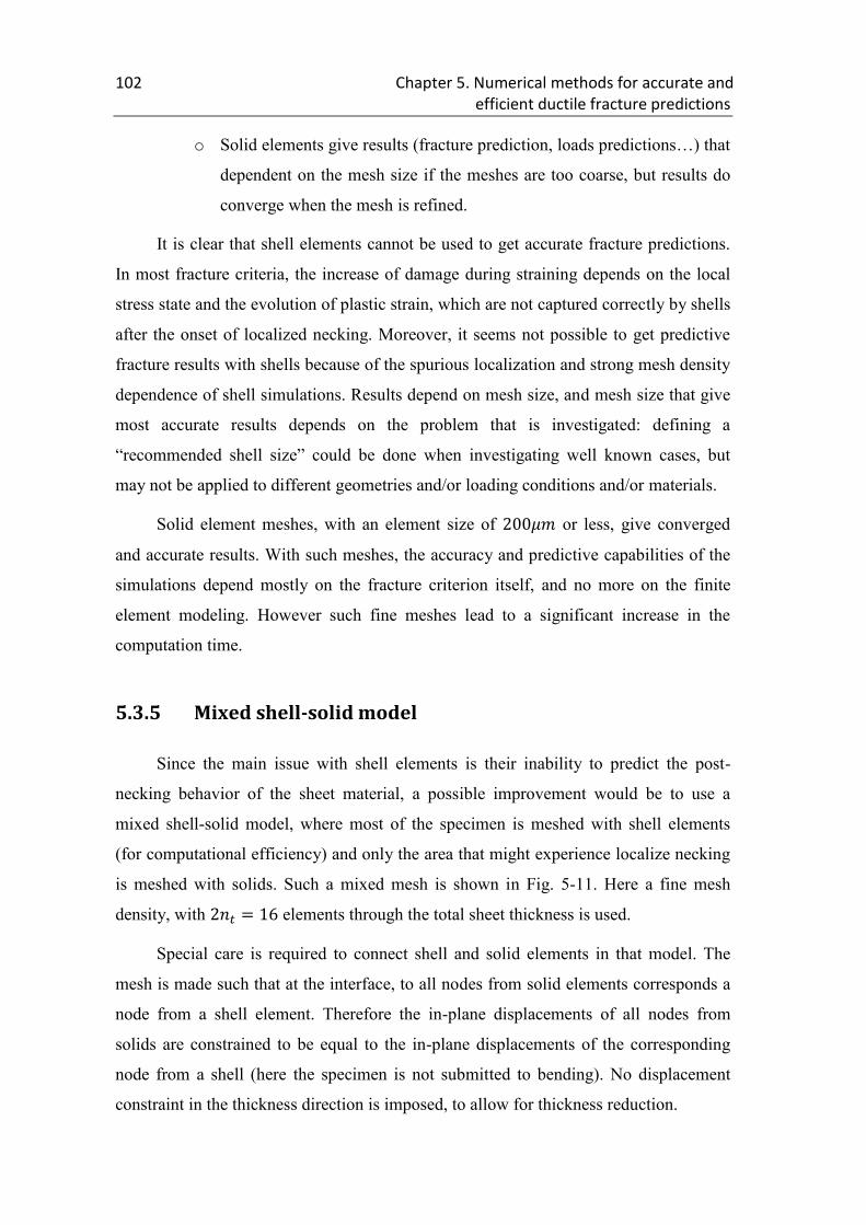
102 Chapter 5. Numerical methods for accurate and efficient ductile fracture predictions
o Solid elements give results (fracture prediction, loads predictions…) that
dependent on the mesh size if the meshes are too coarse, but results do
converge when the mesh is refined.
It is clear that shell elements cannot be used to get accurate fracture predictions.
In most fracture criteria, the increase of damage during straining depends on the local
stress state and the evolution of plastic strain, which are not captured correctly by shells
after the onset of localized necking. Moreover, it seems not possible to get predictive
fracture results with shells because of the spurious localization and strong mesh density
dependence of shell simulations. Results depend on mesh size, and mesh size that give
most accurate results depends on the problem that is investigated: defining a
“recommended shell size” could be done when investigating well known cases, but
may not be applied to different geometries and/or loading conditions and/or materials.
Solid element meshes, with an element size of or less, give converged
and accurate results. With such meshes, the accuracy and predictive capabilities of the
simulations depend mostly on the fracture criterion itself, and no more on the finite
element modeling. However such fine meshes lead to a significant increase in the
computation time.
5.3.5 Mixed shell-solid model
Since the main issue with shell elements is their inability to predict the post-
necking behavior of the sheet material, a possible improvement would be to use a
mixed shell-solid model, where most of the specimen is meshed with shell elements
(for computational efficiency) and only the area that might experience localize necking
is meshed with solids. Such a mixed mesh is shown in Fig. 5-11. Here a fine mesh
density, with elements through the total sheet thickness is used.
Special care is required to connect shell and solid elements in that model. The
mesh is made such that at the interface, to all nodes from solid elements corresponds a
node from a shell element. Therefore the in-plane displacements of all nodes from
solids are constrained to be equal to the in-plane displacements of the corresponding
node from a shell (here the specimen is not submitted to bending). No displacement
constraint in the thickness direction is imposed, to allow for thickness reduction.

5.3. Influence of Finite Element modeling on ductile fracture predictions 103
Figure 5-11: Mixed mesh with local refinement of solid elements.
Figure 5-12: Force displacement curves and fracture predictions using a solid mesh
and a mixed mesh. The experimental instant of fracture is depicted by a dashed black
line.
0
2
4
6
8
10
12
14
16
0 0.5 1 1.5
Forc
e [
kN]
Displacement [mm]
fractureprediction
solid mesh
mixed mesh

104 Chapter 5. Numerical methods for accurate and efficient ductile fracture predictions
Figure 5-13: Evolution of equivalent plastic strain (solid lines) and stress triaxiality
(dashed lines) at the center of the gage section, with a solid mesh (in blue) and a
mixed mesh (in red). The experimental instant of fracture is depicted by a dashed
black line.
Figure 5-12 depicts the force-displacement curves obtained with the fine solid
mesh (in blue) and with the mixed mesh (in red). Both curves lie almost perfectly on
top of each other, demonstrating that the mixed model is able to predict the load
carrying capacity of the specimen, even after the onset of localized necking. Predictions
of the fracture displacement are also very close in both models, only differing by about
3%. Local stress and strain states at the center of the specimen gage section are
depicted in Fig. 5-13 for both models. Even though the evolution of equivalent plastic
strain (solid red line in Fig. 5-13) is similar in both models up to the onset of fracture,
the mixed model tends to underestimate the stress triaxiality (dashed red line in Fig. 5-
13), leading to a different accumulation of damage and, in fine, a slightly different
prediction for the fracture displacement.
The mixed model leads to results that are very close to a full solid model, at a
better computational cost. The CPU time to compute the mixed model is only half that
of the solid model, as shown in Table 5-3. Yet, an obvious limitation of this mixed
0
0.1
0.2
0.3
0.4
0.5
0.6
0.7
0.8
0 0.2 0.4 0.6 0.8 1 1.2
Eq. p
last
ic s
trai
n [
-]
Stre
ss t
riax
ialit
y [-
]
Displacement [mm]
solid mesh
mixed mesh

5.4. Dynamic shell-to-solid re-meshing 105
approach is that one needs to know where localization will occur a priori, in order to
mesh correctly and efficiently the model.
Table 5-3: CPU time (in s) for the solid and mixed models
Solid model Mixed model
2913 1581
5.4 Dynamic shell-to-solid re-meshing
It has been shown that solid elements are required in the post-necking range to
get accurate simulation results and fracture predictions, while shell elements give
satisfactory results before the onset of necking at a much lighter cost. A solution to
reduce further the computation time without compromising the accuracy of the fracture
predictions would thus be to start from a mesh of only shell elements and switch locally
to solid elements where localization is likely to occur. This dynamic re-meshing from
shell to solid elements has been implemented in the explicit Finite Element solver
PamCrash (ESI Group, [144]). The goal of the present section is to perform an
assessment of this re-meshing technique in terms of result accuracy and computational
efficiency.
5.4.1 Principle
The principle of the shell-to-solid re-meshing technique is described in Fig. 5-14,
which corresponds to the simulation of a tension test. Starting from a very coarse shell
mesh (Fig. 5-14a), the shell elements in the specimen gage section are transformed into
finer solid elements when a critical equivalent plastic strain is reached (Fig. 5-14b and
5-14c). All local state variables (stresses, strains…) are automatically mapped from the
integration points of the shell element to the integration points of the new solid mesh.
Note that all the solid elements replacing a single shell elements and located in the
same layer in the sheet plane are initialized with the same value for all state variables

106 Chapter 5. Numerical methods for accurate and efficient ductile fracture predictions
Figure 5-14: Simulation of a tension test using shell-to-solid re-meshing. (a) initial
mesh; (b) Before the re-meshing step; (c) after the re-meshing step and (d) neck
development.
(as can be seen in Fig. 5-14 for the equivalent plastic strain): there is no in-plane
interpolation of the local fields between different integration points. However
interpolation is performed in the through-the-thickness direction, as a shell typically
features multiple integration points through the thickness, which do not necessarily
match the number of generated solids in the thickness direction. This method permits to
correctly account for bending deformations and bending moments during the re-

5.4. Dynamic shell-to-solid re-meshing 107
meshing process. A localized neck is then able to develop within the solid mesh (Fig. 5-
14d).
Shell-to-solid re-meshing has two major effects on computational time:
- It increases significantly the total number of degrees of freedom and element
integration points of the model,
- In an explicit time integration scheme, newly generated solid elements are
associated to a stable time increment much smaller than that of the shell elements
they are replacing, being of smaller dimensions.
In order not to penalize the complete model with a reduced time increment, and
since re-meshing often only concerns a small region of the model geometry, solid
elements are isolated in a separate sub-model. A multi-model coupling technique then
permits to use different time increments for the shell and solid elements [144]. In this
case, nodes located at the interface of shell and solid elements are linked with non-
linear springs, in order to transmit loads and velocities while running on different time
increments.
Plasticity and fracture models defined in Section 5.2, and the routines needed to
map relevant variables (stresses, strains, damage indicator) from shell elements to solid
elements during re-meshing have been implemented into the Finite Element software
PamCrash to carry out the work described thereafter.
5.4.2 Simple example
Before analyzing complex fracture problems, we start by evaluating the shell-to-
solid re-meshing technique on a simulation of a simple tension test on a sheet
specimen, as shown in Fig. 5-14.
5.4.2.1 Numerical model and results
The initial shell model of the tension specimen is depicted in Fig. 5-14a. The
gage section is 30mm long and 10mm wide and is meshed with only three shell
elements. To load the specimen, displacements are imposed to one boundary, while the
other is fixed. A non-associated quadratic plasticity model, as described in section 5.2,

108 Chapter 5. Numerical methods for accurate and efficient ductile fracture predictions
is used along with the material parameters given in Table 5-1. No fracture criterion is
used so far.
The shell-to-solid re-meshing option is activated. When an equivalent plastic
strain of is reached at any integration point of a shell element, it is replaced
by solids. Each re-meshed shell is decomposed into 4 solid elements in each in-plane
direction, and 4 elements in the thickness direction, as shown in Fig. 5-14c.
The resulting load-displacement curve is depicted with a blue line in Fig. 5-15.
The instant when re-meshing occurs is characterized by a significant spike in the
applied load, followed by an almost complete drop of the load. The applied load comes
back to the level before re-meshing only after an additional imposed displacement of
about 0.2mm. In between, the model deforms purely elastically. After some plastic
deformation of the generated solid elements, a diffuse and then localized neck forms in
the solid mesh, as visible in Fig. 5-14d. This neck leads to a smooth decrease of the
applied load, as described in the previous section.
During the re-meshing step, springs that link shell and solid models are created
with zero internal load, while they replace material that was loaded up to its yielding
point. Therefore this transient behavior corresponds to a transfer of load between the
initially unloaded springs and the elastically loaded shell and solid elements. It ends
when the model reaches equilibrium, i.e. when the level of load applied before re-
meshing is attained.
The evolution of the kinetic energy in the model in shown in Fig. 5-16. Clearly,
the total kinetic energy is higher after re-meshing. This additional energy comes from
the additional mass introduced by the springs created to link the shell and solid
elements models. In this specific simulation, the mass of the springs (which is chosen
automatically by the solver based on stability criteria) is twice the mass of the
generated solid elements. In addition a transient period exists right after re-meshing,
where the kinetic energy in the solid model exhibits very large oscillations. This
transient corresponds to the time the springs initialized with a zero velocity need to
reach equilibrium (constant non-zero velocity). Note that a constant velocity is imposed
to the boundaries of the model.

5.4. Dynamic shell-to-solid re-meshing 109
Figure 5-15: Force displacement curve of a tensile test with re-meshing, with (red) or
without (blue) pre-load and damping.
Figure 5-16: Evolution of the model kinetic energy.

110 Chapter 5. Numerical methods for accurate and efficient ductile fracture predictions
5.4.2.2 Influence of modeling parameters
Different parameters are implemented to reduce the transient following the re-
meshing step:
- Pre-load can be introduced in the springs,
- Proportional damping and non-linearity can also be introduced in the spring
behavior.
An initial load is introduced in the springs linking nodes from the shell model and
nodes from the solid model. The pre-load is chosen equal to the contribution to the
nodal force coming from elements that are being re-meshed at the instant of re-
meshing. In addition, proportional damping in the spring permits to reduce the
oscillations of kinetic energy visible in Fig. 5-15. The force-displacement curve
obtained using both pre-load and damping is shown in red in Fig. 5-15. The drop of
force at the instant of re-meshing, as well as resulting oscillations, are significantly
reduced.
Similarly, defining a non-linear behavior for the spring (so that the spring load is
no more proportional to its elongation) can help reduce the transient to a small extent.
This type of behavior penalizes an excessive extension or compression of the spring.
However it has been found that using a non-linear behavior has much less influence on
the transient than pre-loading the spring or using damping.
5.4.3 Application to basic fracture experiments
The next step in assessing the performances of the re-meshing technique consists
of comparing its predictions against real fracture experiments.
5.4.3.1 Experiments
We use experimental results described in [48]. In this work, tensile experiments
have been performed on three different specimen geometries sketched in Fig. 5-17:
notched tensile specimens with a notch radius of and ,
respectively, and a tensile specimen with a diameter central hole. The central

5.4. Dynamic shell-to-solid re-meshing 111
Figure 5-17: Flat tensile specimens with different notched radii and with a central hole.
hole specimen permits to characterize the onset of ductile fracture under a state of
uniaxial tension, while notched tensile specimens allow for fracture characterization
under higher triaxialities. All experiments are performed on a TRIP780 Advanced High
Strength steel sheet, whose material characterization is given in Table 5-1.
5.4.3.2 Numerical models
For each specimen, we consider three different numerical simulations:
1. The geometry is meshed with a coarse mesh of shell elements (as described in
Section 5.3: shells are long in each direction). The re-meshing
capability is switched off.
2. The geometry is initially meshed the shell elements, with the same density as in
case 1. The re-meshing capability is switched on: when an equivalent plastic
strain of 0.18 is reached at any integration point of a shell, this element and its
neighbors (in a region of 5mm radius) are replaced by solid elements. Each
shell is replaced by 4x4 solid elements in both in-plane directions, and 16
elements in the thickness direction. The density of solid elements corresponds

112 Chapter 5. Numerical methods for accurate and efficient ductile fracture predictions
Figure 5-18: Contour plot of equivalent plastic strain in a notched tensile
specimen after re-meshing of the gage section center. Central elements have already
failed.
to that of the fine mesh described in Section 5.3, with an in-plane length of
and thickness of .
3. The geometry is meshed with solid elements only. The density corresponds to
the one obtained after re-meshing in case 2.
We make use of the modeling parameters that have been recommended
previously for the re-meshing operation. In all simulations, element deletion is
performed when a damage value of 1.0 is reached at any integration point of an
element.
5.4.3.3 Results and discussion
Figure 5-18 shows the result of the re-meshing procedure for the
notched tensile specimen. All the shell elements located at the center of the gage

5.4. Dynamic shell-to-solid re-meshing 113
Figure 5-19: Predicted force displacement curve of the notched tensile test with
re-meshing. The experimental instant of fracture is depicted by a dashed black line.
Figure 5-20: Predicted force displacement curve of the notched tensile test with
re-meshing. The experimental instant of fracture is depicted by a dashed black line.

114 Chapter 5. Numerical methods for accurate and efficient ductile fracture predictions
Figure 5-21: Predicted force displacement curve of the central hole tensile test with re-
meshing. The experimental instant of fracture is depicted by a dashed black line.
section have been replaced by very fine solid elements. The picture is taken after the
onset of fracture (crack initiation), and before the complete failure of the specimen:
deleted elements (which correspond to a small crack) can be spotted at the center of the
specimen, where the plastic strain is the highest.
Load-displacement curves predicted for the three geometries are depicted in Figs.
5-19 to 5-21. Results using shell elements only (case 1) are in blue, solid elements (case
3) in red and results using re-meshing (case 2) are in green. In all simulations, the
abrupt drop of force corresponds to the onset of fracture, while small oscillations
visible on the results of simulations using re-meshing (green lines in Figs. 5-19 to 5-21)
correspond to re-meshing steps as explained in Section 5.4.2. In addition to the
predicted load-displacement curves, the experimental instant of fracture is depicted
with a black dashed line for the three geometries. For all geometries, the load-
displacement curve features a maximum of force before fracture, which corresponds to
the onset of through-the-thickness localization of the stress and strain fields within the
specimen gage sections.

5.4. Dynamic shell-to-solid re-meshing 115
For the three fracture experiments considered, simulations using fine solid
elements (case 3) predict the instant of fracture with a very good accuracy. As already
detailed in section 5.4, simulations using shell elements always under-estimate the
fracture displacement. In fact in shell simulations failure occurs just after the maximum
of force is reached, as those elements cannot capture correctly the post-necking
behavior of the sheet material. When using shell-to-solid re-meshing (green curves in
Figs. 5-19 to 5-21), fracture occurs later than when only solid elements are used (red
curves). The fracture displacement is over-estimated by 4% for the notched
tensile specimen, by 7% for the notched tensile specimen and by 5% for the
specimen with a central hole. Note that with re-meshing, simulations with initially only
shell elements are able to predict correctly the applied load after its maximum.
The evolution of equivalent plastic strain, stress triaxiality and damage at the
integration point which fails first are depicted in Figs. 5-22 to 5-24, for the
notched tensile specimen. Results from the simulation with solid elements only are
shown in red while results using re-meshing are in green. Note that two major re-
meshing steps occur in that simulation, the first one at a displacement of about
Figure 5-22: Evolution of equivalent plastic strain at the center of the notched
tensile specimen, predicted using a solid mesh or re-meshing.

116 Chapter 5. Numerical methods for accurate and efficient ductile fracture predictions
Figure 5-23: Evolution of stress triaxiality at the center of the notched tensile
specimen, predicted using a solid mesh or re-meshing.
Figure 5-24: Evolution of damage at the center of the notched tensile specimen,
predicted using a solid mesh or re-meshing.

5.4. Dynamic shell-to-solid re-meshing 117
where approximately 41,000 solid elements are generated at the center of the gage
section, and a second step at a displacement of about where 10,000 new solid
elements are added to extend the re-meshed area. Before the first re-meshing step, i.e.
when only shell elements are present, both the equivalent plastic strain (in Fig. 5-22)
and the stress triaxiality (in Fig. 5-23) are underestimated at the center of the gage
section compared to results from solid elements (simulation #3, in red). As a result, at
the instant of the first re-meshing step, the damage indicator is lower by 15% than in
the simulation with only solids. After re-meshing, i.e. when the the center of the
specimen gage section is meshed with solid elements, the evolution of equivalent
plastic strain is comparable in both simulations: when shifted by the offset due to the
inaccuracy of shells, the curve from the re-meshing simulation (in blue in Fig. 5-22)
lies almost exactly on top of the curve from the solid simulation (in red in Fig. 5-22).
Only a small discrepancy is noticeable at the instant of the second re-meshing step.
The evolution of stress triaxiality (Fig. 5-23) is also slightly underestimated by
shell elements before the first re-meshing step. However, unlike for the equivalent
plastic strain, differences between the solid simulation and the re-meshing simulation
are significant after re-meshing occurred. In particular significant drops of the
triaxiality occur at each re-meshing step. Those drops in the stress state correspond to
the transient period following the re-meshing step described in Section 5.4.2. In spite of
those local drops, it can be noted that the re-meshing simulation is able to capture the
increase of triaxialty due to localized necking that occurs before fracture.
Therefore it can be concluded that the over-estimation of the predicted fracture
displacement in the simulation with re-meshing is due to under-estimation by shell
elements of the plastic strain, stress triaxiality and damage in the early stages of the
simulation (before the first re-meshing step) and, to a small extent, to partial unloading
that occurs during the subsequent re-meshing steps.
CPU times for the three geometries, using only solid elements and with re-
meshing, are summarized in Table 5-4. Note that in all cases, the computation time is
reduced by about 75% when re-meshing is used. However it is still much more than
when using shell elements only. For all three geometries, the number of generated solid
elements is very large compared to the initial number of shells elements. Therefore the
computation is controlled by the sub-model containing the generated solids. In case of a

118 Chapter 5. Numerical methods for accurate and efficient ductile fracture predictions
simulation of a larger part, where the ratio of generated solids to shell elements would
be smaller, it is obvious that the time savings using re-meshing would be greater.
Table 5-4: CPU time (in s) when using re-meshing
Geometry notch notch Central hole
Re-meshing 32,300 40,900 52,300
Only solid 126,800 129,800 204,900
5.5 Conclusion
In this chapter, the influence of spacial discretization of Finite Element models on
ductile fracture predictions in sheet metals has been investigated. In addition, possible
improvements coming from dynamic shell-to-solid re-meshing during the simulations
have been assessed.
Based on numerical simulations of a tensile experiment on a flat specimen with
circular notches using different element types (both shells and solids) as well as
different mesh densities, it has been shown that shells cannot predict the post-necking
behavior of sheet materials, regardless of mesh density. As a result spurious
localization occurs at the onset of necking, leading to premature failure of the
specimen. On the other hand, solids elements are able to predict the through-the-
thickness localization that occurs before ductile fracture in AHSS, and thus allow for
accurate predictions of the onset of ductile fracture when used in conjunction with
suitable fracture initiation models. However very fine meshes (with an element length
of about ) are required in order to get converged8 numerical results: improved
accuracy comes at the expense of computational efficiency.
Automatic re-meshing of shell into solid elements is considered to improve the
accuracy of simulations with shell elements. The accuracy of the re-meshing technique
is evaluated based on numerical simulations of tensile fracture experiments and
8 In the sense that using a finer mesh would not change the numerical results.

5.5. Conclusion 119
comparison of numerical predictions to experimental results. Concerning the prediction
of the onset of ductile fracture, it is shown that simulations with re-meshing are more
accurate that those with shell elements only. However, simulations with re-meshing do
not match the accuracy of simulations with solid elements only. It is worth mentioning
that most of the inaccuracy originates in the first stages of the simulations, before re-
meshing when the mesh is composed by shell elements only. In addition, re-meshing
permits to predict correctly the post-necking behavior of sheet materials, which cannot
be done with shell elements. A correct prediction of local material state of deformation
and stress is necessary when trying to predict crack orientation and propagation.


Chapter 6
Analysis of the failure micro-mechanisms
Contents
6.1 Introduction .................................................................................................. 122
6.2 Macroscopic analysis: experiments and simulations ................................... 122 6.2.1 Notched tension experiments ............................................................... 123 6.2.2 Tension on a specimen with a central hole ......................................... 126
6.2.3 Punch Experiment ............................................................................... 129 6.2.4 Dependence of the strain to fracture on stress state ........................... 129
6.3 Fractographic analysis .................................................................................. 130 6.3.1 Sample preparation ............................................................................. 130
6.3.2 Microscopic observations of polished cross-sections ......................... 131 6.3.3 Fracture surfaces ................................................................................ 137
6.3.4 Effect of strain rate on damage ........................................................... 137
6.4 Mechanical interpretation of the observations ............................................. 137
6.5 Conclusion .................................................................................................... 139
Abstract
The evolution of damage and the mechanisms responsible for ductile failure are
identified in the TRIP steel sheet submitted to different stress states, using optical and
scanning electron microscopy. Experiments are performed on tensile specimens and on
disk specimens submitted to out-of-plane hemispherical punching, thereby covering
stress states from uniaxial to equi-biaxial tension. For each specimen geometry,
experiments have been interrupted prior to fracture at different stages of deformation:
onset of through the thickness necking and 95%, 99% of the displacement at which
fracture initiates. Micrographs of samples extracted from the deformed specimens
permit to evaluate the material damage for increasing amounts of accumulated plastic
strain, and identify rupture mechanisms. It is shown that the critical mechanism
9 This Chapter is reproduced from: Dunand M., Mohr D. and Ravi-Chandar K., “Shear fracture of
Advanced High Strength Steels: Mechanism Analysis and Micromechanical modeling”. Submitted.

122 Chapter 6. Analysis of the failure micro-mechanisms
responsible for material failure is the localization of the plastic deformation in a shear
band initiating at a grown and isolated void. The orientation of the fracture surface is
controlled by the shear band direction.
6.1 Introduction
Damage mechanisms leading to ductile failure are generally described in terms of
void nucleation, void growth and finally void linkage that form cracks. An extensive
review of ductile fracture mechanisms can be found in Garrison and Moody (1987,
[63]). Observation and characterization of damage mechanisms is traditionally done by
means of optical and Scanning Electron microscopy. This destructive approach only
gives access to two-dimensional information. High resolution tomography and
laminography are now increasingly used for non-destructive three-dimensional
observation of damage in metallic materials (e.g. Morgeneyer et al, 2008, [128]; Maire
et al., 2012, [117]).
In this Chapter, attention is limited to studying the mechanisms leading to ductile
failure under biaxial tension, i.e. plane stress states between uniaxial tension and equi-
biaxial tension. A series of interrupted tensile experiments is performed on specimens
extracted from TRIP780 steel sheets. A specimen with a central hole is used to study
uniaxial tension, while notched flat specimens cover intermediate stress states in the
vicinity of plane strain tension. In addition, interrupted punch experiments are
performed to investigate the failure mechanism under equi-biaxial tension. Micrographs
of specimens corresponding to different stages of loading prior to failure are analyzed
in view of void nucleation and growth as well as localization of plastic deformation at
the grain level. The experimental observations suggest that shear band formation is the
governing failure mechanism under biaxial tension.
6.2 Macroscopic analysis: experiments and simulations
Different experiments are performed to shed some light on the fracture
mechanism at stress states in the vicinity of biaxial tension. A finite element simulation

6.2. Macroscopic analysis: experiments and simulations 123
is performed of each experiment to provide access to the local stress and strain fields
inside the specimen. The reliability of the numerical simulation and the underlying
plasticity model is not demonstrated here as it is covered by previous publications on
this material (Dunand and Mohr (2010, 2011, [48-50]) and Mohr et al. (2010, [122])),
as well as in Chapter 5. Instead, we focus on describing the experimental and numerical
results at the macroscopic level in the present section, before moving to the
microscopic level in the sequel.
6.2.1 Notched tension experiments
Tensile experiments are performed on flat notched specimens (Fig. 6-1a).
Specimens are 20mm wide in the shoulder area and feature a minimum width of 10mm
at the center. The notch radius is R=6.65mm. Experiments are carried out under
displacement control at a constant crosshead velocity of 0.5mm/min. Planar Digital
Image Correlation (2D-DIC) is used to measure the relative displacement of the
specimen boundaries and the displacement field at the center of the gage section.
(a) (b)
Figure 6-1: Tensile specimens with (a) a notch radius 6.65mm and (b) tensile
specimen with central hole. Red marks depict the position from where micrography
samples are extracted.

124 Chapter 6. Analysis of the failure micro-mechanisms
(a)
(b)

6.2. Macroscopic analysis: experiments and simulations 125
(c)
Figure 6-2: Force displacement curves of the (a) notched tensile experiment, (b)
central hole tensile experiment and (c) punch experiment.
The measured force-displacement curve is depicted in black in Fig 6-2a. A force
maximum is reached before fracture occurs, roughly corresponding to the instant of the
onset of through-the-thickness necking. Beyond the onset of necking, steep gradients in
the stress and strain fields develop both in-plane and through-the-thickness at the center
of the specimen gage section (Fig. 6-3).
The plane stress condition prevail up to the onset of through-thickness necking.
Thereafter, a stress in specimen thickness direction builds up. The corresponding plots
of the estimated loading paths at the specimen center, i.e. the evolution of the
equivalent plastic strain as a function of the stress triaxiality and the Lode angle
parameter, therefore show a pronounced kink associated with necking followed by an
increase in stress triaxiality and a decrease in the Lode angle parameter (Fig. 6-4). The
reader is referred to Dunand and Mohr (2010, [48]) for more details on the numerical
model.

126 Chapter 6. Analysis of the failure micro-mechanisms
Figure 6-3: Contour plot of the equivalent plastic strain at the instant of the onset of
fracture in a notched specimen.
In addition to the monotonic experiment all the way to fracture, the experiment is
repeated for additional specimens, but interrupted prior to fracture at different stages of
deformation: maximum of force; 95% and 99% of the displacement at which fracture
initiates. Due to the excellent repeatability of the experiments for the material at hand,
the corresponding force-displacement curves lie on top of each other (Fig. 6-2a). The
end points of the interrupted experiments are therefore highlighted by a triangle symbol
in Fig. 6-2a and 6-4.
6.2.2 Tension on a specimen with a central hole
In close analogy with the experimental program on the notched tension specimen,
experiments are performed on a tensile specimen with a central hole (Fig. 6-1b). The
hole has a diameter of 8mm while the ligaments to the left and right of the hole are each
6mm wide. Following exactly the same procedure as for the notched specimen, a
monotonic experiment is performed all the way to fracture, followed by a series of

6.2. Macroscopic analysis: experiments and simulations 127
(a)
(b)
Figure 6-4: Loading paths to fracture. (a) Evolution of equivalent plastic strain versus
stress triaxiality and (b) evolution of equivalent plastic strain versus Lode angle. Solid
points depict the onset of fracture.

128 Chapter 6. Analysis of the failure micro-mechanisms
interrupted experiments ending at maximum of force and 99% of the displacement of
total failure, respectively. Corresponding force-displacement curves are shown in Fig.
6-2b.
The cracks are assumed to initiate near the boundary of the central hole. The
corresponding finite element simulation shows that through-thickness necking occurs in
the hole ligaments, with the strongest thickness reduction of up to 38% at a distance of
0.9mm from the hole boundary. The evolution of the stress state at an integration point
located at the specimen mid-plane near the hole boundary is shown in Fig. 6-4. Due to
the proximity to the hole boundary, the stress state remains close to uniaxial tension all
the way to fracture, i.e. the stress triaxiality and Lode angle parameter are close to 0.33
and 1.0, respectively. Selected views of the deformed FEA mesh at the instant of onset
of fracture are shown in Fig. 6-5 with a contour plot of the axial plastic strain.
Figure 6-5: Specimen with a central hole: contour plot of plastic axial strain at the
instant of the onset of fracture.

6.2. Macroscopic analysis: experiments and simulations 129
6.2.3 Punch Experiment
In order to characterize the material response for equi-biaxial tension, a sheet
specimen is clamped on a circular die and subsequently loaded through a hemispherical
punch. The punch and die have a diameter of 44.5mm and 100mm, respectively. The
clamping pressure is applied through eight M10-12.9 screws. The experiment is carried
out on a screw-driven universal testing machine (MTS, Model G45) at a constant punch
velocity of 5mm/min. In order to limit the effects of friction, a stack of six oil-
lubricated 90µm thick Teflon layers is put between the specimen and the punch during
each test. Three-dimensional Digital Image Correlation is used to measure the out-of-
plane deformation of the specimen. The applied force versus punch displacement curve
is depicted in black in Fig. 6-2c; it increases monotonically until a sharp drop in the
force level is observed at the instant of the onset of fracture. Fracture occurs at the top
of the dome, where the stress state is close to equi-biaxial tension.
As for the tensile experiments, we also carry out interrupted punch experiments
where loading was stopped at 95% and 99% of the punch displacement at which
fracture initiates. Corresponding superposing force-displacement curves are shown in
Fig. 6-2c with triangle-symbols indicating the points of interruption. The
accompanying finite element simulations shows the absence of through-thickness
necking. As a result, the loading path to fracture remains more or less proportional, i.e.
both the stress triaxiality and the Lode angle parameter remained constant at 0.66 and -
1.0, respectively.
6.2.4 Dependence of the strain to fracture on stress state
The results from the above experiments along with the computational analysis
provide insight into the stress state dependency of the strain to fracture. Here, the
“strain to fracture” is defined as the largest achievable macroscopic strain prior to the
formation of cracks or narrow bands of localization of plastic deformation. This
definition is very useful from an engineering point of view. From a physical point of
view, it might be more meaningful to define the strain to fracture at smaller length
scale. For instance, in polycrystalline materials, it could be associated with the plastic
deformation at the grain level up to the point of micro-crack formation. Clearly, the use

130 Chapter 6. Analysis of the failure micro-mechanisms
of the latter definition would require more involved material models that can predict the
strains at the grain level.
Taking a purely phenomenological macroscopic approach (see discussion in
Section 2.2), stress triaxiality and Lode angle parameter dependent damage indicator
models have been developed recently to describe the effect of stress state on the strain
to fracture (e.g. Bai and Wierzbicki, 2010, [7]; Mohr and Marcadet, 2012, [125]). For
biaxial tension, these models predict a minimum in the strain to fracture for transverse
plane strain tension, while the strain to fracture is supposed to increase monotonically
towards the respective limiting cases of uniaxial tension and equi-biaxial tension. It is
the goal of the subsequent two sections, to provide a physics-based explanation of this
characteristic drop in the strain to fracture for plane strain tension.
6.3 Fractographic analysis
6.3.1 Sample preparation
Cross-sectional cuts are prepared from the tested specimens for microscopic
inspection. For the tensile experiments (notched and central hole specimens), the
observation plane is the one containing the axial and thickness directions. A red solid
line in Fig. 6-1 indicates the projection of the observed cross-sections on the specimen
surface. For the punch experiment, the observation plane includes the thickness and
transverse sheet direction, since the first cracks always formed parallel to the sheet
rolling direction.
The sheet cutting is done using a wire saw. The samples preparation follows
closely the procedure described in the Metals Handbook vol.8 (1990, [5]). The samples
are first mounted in a conductive phenolic mounting compound filled with aluminum
particles. They are then ground and polished. The final polishing step is performed with
a diamond paste. Etching is finally performed using a 2% Nital solution.

6.3. Fractographic analysis 131
6.3.2 Microscopic observations of polished cross-sections
A series of micrographs of the notched tensile specimens is shown in Fig. 6-6 as
recorded with the Back-Scattered Electron (BSE) detector of a FEI XL40 scanning
electron microscope operating at . According to our finite element analysis, the
corresponding accumulated equivalent plastic strains at the specimen center are:
(maximum force, Fig. 6-6a), (95% displ., Fig. 6-6b) and
(99% displ., Fig. 6-6c).
At maximum force (Fig. 6-6a), the specimen already exhibits noticeable damage in
the form of voids. The area fraction of voids is about 4x10⁻³
in Fig. 6-6a, while virtually
no voids are visible in the undeformed material (Fig. 1-1). The position of the voids
suggests that they nucleated at the ferrite/martensite and/or ferrite/austenite grain
boundaries. Strain incompatibilities between the different phases may induce more
rapid debonding at the phase interfaces (Jacques et al., 2001, [87]). Moreover, most of
the visible voids are aligned parallel to the loading direction (which also coincides with
the sheet rolling direction). Lorthios et al. (2010, [114]) observed similar nucleation
patterns in TWIP steels by means of x-ray tomography. Note that the undeformed
material shows segregation bands of austenite (Fig. 1-1), which seem to be favored
sites for void nucleation. Some voids have also nucleated away from the segregation
bands at apparently random locations in the specimens.
Figure 6-6b (0.95 ) shows a polished cross-section for significantly higher
equivalent plastic with an estimated maximum of at the specimen center. At
this stage of deformation, the area fraction of voids has increased to about 7.4x10⁻³
.
However, it is important to note that the average size of the voids is very similar to that
of the voids observed at maximum force. In other words, the measured increase in void
volume fraction is not due to void growth. Instead, it is due to additional void
nucleation. Based on x-ray tomography quantitative observations made on a DP600
steel sheet and its phase constituents, Maire et al. (2008, [116]) and Bareggi et al.
(2012, [12]) also concluded that the average void diameter does not increase during
straining, while additional damage is mainly due to the nucleation of new cavities. At
0.95 , the observed void alignments are longer than those at maximum force. Voids

132 Chapter 6. Analysis of the failure micro-mechanisms
(a)
(b)

6.3. Fractographic analysis 133
(c)
Figure 6-6: SEM micrographs from notched tensile experiments interrupted at (a) the
maximum of force, (b) 95% of the displacement to fracture and (c) 99% of the
displacement to fracture. The L and Th orientations correspond to the specimen
loading direction and through-the-thickness direction, respectively.
seem to nucleate at both ends of the alignments. Void coalescence is also observed
among voids within the same alignment, thereby forming microcracks parallel to the
loading direction.
At 99% of the displacement to fracture, the observed mesostructure is similar to
that at 95% of the displacement to fracture. However, at a higher magnification, the
inspection of martensite grain bands (bright phase in Fig. 6-6c) shows signs of shear
cracks. The martensite grains are organized in more or less straight bands along the

134 Chapter 6. Analysis of the failure micro-mechanisms
(a)
(b)

6.3. Fractographic analysis 135
(c)
Figure 6-7: Cross sections of post-mortem specimens of (a) notched tensile
experiment, (b) central hole experiment and (c) punch experiment.
rolling direction. Two such bands have been highlighted by red dashed lines in Fig.
6-6c. Prior to the fracture of the entire specimen (i.e. at 99% displ.), a tangential and
normal discontinuity becomes apparent in the martensite bands. Figure 6-6c also shows
a large hole at the top left which is disregarded because we think that it is just the trace
of grains that have been torn out during polishing.
We note that remarkably similar observations are made when analyzing the
corresponding cross-sectional cuts for tension with a central hole and even for the
punch specimen. The corresponding micrographs of interrupted specimens are therefore
not shown for conciseness. The longitudinal cross sections of the fractured notched and
punch specimens all show straight slanted cracks (Fig. 6-7). In particular, the fracture
surface is inclined at an angle of about 45° with respect to plane of the sheet. The only

136 Chapter 6. Analysis of the failure micro-mechanisms
(a)
(b)
Figure 6-8: SEM fractographs from a broken notched tensile specimen. The Th and Tr
orientations correspond to the through-the-thickness and specimen transverse
directions, respectively.

6.4. Mechanical interpretation of the observations 137
exception is the central hole specimen, which features a V-shaped fracture surface (Fig.
6-7b).
6.3.3 Fracture surfaces
SEM fractographs from a notched tensile specimen are presented in Fig. 6-8. The
fracture surface presents a dimple pattern with a dimple size of about (Fig. 6-8b).
The eccentricity of the black apex of the dimples with respect to the bright
circumference (Fig. 6-8b) suggests that the ellipsoidal dimples are inclined towards the
thickness direction. At a smaller magnification (Fig. 6-8a), the fracture surface features
continuous dark lines of narrow valleys that are parallel to the specimen surface. It
resembles a laminate with multiple layers of to thickness. The layer
thicknesses are similar to the distances between the void bands observed in the cross-
sectional cuts. It is speculated that these valley lines corresponds to the intersection of
the crack surface with the void necklaces.
6.3.4 Effect of strain rate on damage
Even though technological solution are available to perform interrupted
experiments in Split Hopkinson Bar systems (e.g. Nemat-Nasser et al., [134]), it has not
been implemented as part of this thesis. Damage mechanisms taking place at high strain
rate are thus not formally identified. However, fracture surfaces and cross-sections of
post-mortem specimens submitted to high strain rate loadings are similar to those
describes hereinabove. It is therefore assumed that damage mechanisms are comparable
at low and high strain rates.
6.4 Mechanical interpretation of the observations
Based on the above observations, the following comments with regards to the
mechanism leading to ductile fracture under biaxial tension can be made:
1. Voids nucleate at ferrite/martensite and ferrite/austenite grain boundaries,
preferably along alignments parallel to the specimen loading direction

138 Chapter 6. Analysis of the failure micro-mechanisms
Nucleation takes place before necking, i.e. at zero out-of-plane stress. At this
stage, the plastic strains are small ( ) as compared to those reached at
the onset of fracture ( ).
2. The void volume fraction increases mostly because of new nucleations (and not
due to the growth of existing voids).
3. Through-thickness necking is just a structural deformation mode which
localizes the deformation to a small zone within the specimen. At the length
scale associated with necking (sheet thickness), the material can still be
considered as a homogenous continuum.
4. The local increase in stress triaxiality due to necking has no noticeable effect on
the size of the voids. Furthermore, a similar void size is observed for tension
with central hole (triaxiality of 0.33), notched tension and in a punch
experiment (triaxiality of 0.66).
5. Coalescence occurs within void alignments (necklace mechanism) thereby
forming microcracks parallel to the specimen loading direction. However, it
appears that those microcracks and voids do not compromise the material’s
load carrying capacity along the axial direction.
6. Voids acts as material imperfections that trigger the localization of the plastic
flow into a narrow band of localized plastic deformation. At this stage, a
homogeneous description of the material is expected to become invalid. Due to
the 45° orientation of the final fracture surface with respect to the axial
direction, shear localization is considered as the dominant mechanism of plastic
localization.
7. Secondary voids nucleate within the band of localized plastic deformation. The
secondary voids eventually coalesce and create a macroscopic crack,
independent of the microcracks associated with the necklace mechanism.
Among all steps involved in the ductile fracture process, we consider the
localization of deformation in a narrow band as the most important precursor at the
macroscopic level before cracks are formed at the grain level. It is worth noting that
already more than 30 years ago, researchers considered shear localization as the

6.5. Conclusion 139
dominant mechanism leading to fracture of metals (e.g. Rice, 1976, [151]). On the other
hand, the role of void growth and void shape changes appears to be secondary. These
effects are probably only important within the band of localized deformation where
other material heterogeneities (grain anisotropy and grain boundaries) may also come
into play.
6.5 Conclusion
Damage mechanisms responsible for ductile failure of the TRIP steel at low strain
rate have been characterized. Selected experiments, covering all the range of biaxial
stresses, are carried out and interrupted at different levels of deformation. Samples
extracted from the deformed specimens are analyzed by means of Optical and Scanning
Electron Microscopy in order to identify the evolution of damage mechanisms.
Observations show that interfaces between ferrite and martensite grains constitute
preferred sites for void nucleation, which occurs at relatively low strains. However,
void growth is not significant for all stress states considered. Damage increases mostly
through nucleation of new cavities during deformation. It is found that the critical
mechanism leading to fracture is a localization of the plastic flow at the grain scale into
a planar band of shear deformation.


Chapter 7
Modeling of the failure mechanisms
Contents
7.1 Introduction .................................................................................................. 142
7.2 Micromechanical modeling ......................................................................... 146 7.2.1 3D unit cell model geometry and boundary conditions ...................... 147 7.2.2 Macroscopic rate of deformation tensor ............................................ 149
7.2.3 Control of the macroscopic stress state .............................................. 150 7.2.4 Stress orientation evolution ................................................................ 153
7.2.5 Computation of the onset of localization for a given stress state ....... 154
7.3 Simulation results ........................................................................................ 155
7.3.1 Onset of localization ........................................................................... 155 7.3.2 Effect of anisotropy ............................................................................. 159
7.3.3 Influence of the biaxial stress ratio on localization ............................ 162 7.3.4 Influence of the defect volume fraction ............................................... 164
7.4 Rate-dependent localization analysis ........................................................... 166
7.5 Conclusion ................................................................................................... 170
Abstract
A numerical model is developped to investigate the influence of the stress state
and strain rate on the onset of localization of the plastic flow in a void-containing
material. A three-dimensional unit cell containing an initially spherical void is
submitted to proportional loadings in the macroscopic stress space. Fully periodic
boundary conditions are applied. The range of stress states considered are limited to
biaxial tension, i.e. from uniaxial to equi-biaxial tension under plane stress conditinos.
The model is able to predict qualitatively the dependence of ductility to the stress state
observed experimentaly, as well as the increase of ductility at high strain rate.
10
This Chapter is reproduced from: Dunand M., Mohr D. and Ravi-Chandar K., “Shear fracture of
Advanced High Strength Steels: Mechanism Analysis and Micromechanical modeling”. In preparation.

142 Chapter 7. Modeling of the failure mechanisms
7.1 Introduction
The localization of plastic deformation within a narrow band is often an important
precursor to ductile fracture. Following the works of Marciniak and Kuczynski (1964,
[118]) and Rice (1977, [151]), it is common practice to predict the onset of localization
based on macroscopic constitutive theories through infinite band localization analysis
(e.g. Mear and Hutchinson, 1985, [120], Duszek and Perzyna, 1991, [53]). As noted by
Rice (1977, [151]), the identified onset of localization corresponds to the loss of
ellipticity of the governing equilibrium equations. Consequently, onset of localization
maps can also be directly computed by assessing the loss of ellipticity of incremental
moduli (Michel et al., 2007, [121]; Danas and Ponte Castaneda, 2012, [42]).
For most metals, the strains at the onset of localization are very large. As a
consequence, the effect of voids on the elasto-plastic moduli, even for very low
porosities, needs to be taken into account when computing the instant of the onset of
localization. This requires advanced constitutive theories such as the Gurson model
(Gurson, 1977, [70]) and its extensions accounting for void nucleation (e.g. Chu and
Needleman, 1980, [35]), for the loss of load-carrying capacity associated with void
coalescence (e.g. Tvergaard and Needleman, 1984, [181]), for void shape effects (e.g.,
Gologanu et al., 1993, 1994, [67, 68]; Garajeu et al., 2000, [62]; Pardoen and
Hutchinson, 2000, [146]) and for plastic anisotropy (e.g., Benzerga et al., 2004, [18]).
As shown by Nahshon and Hutchinson (2008, [130]), additional modifications
representing shear softening are necessary to obtain reasonable predictions of strain
localization at low stress triaxialities.
Unit cell models provide a computationally-expensive alternative to macroscopic
constitutive theories to describe the large deformation response of metals of low
porosity. The early analysis with unit cell models was mostly limited to two-
dimensional models, e.g. axisymmetric mechanical systems with spheroidal voids (e.g.
Koplik and Needleman, 1988, [97]; Brocks et al, 1995, [21]; Pardoen and Hutchinson,
2000, [146]) or plane strain models with cylindrical voids (e.g. Tvergaard, 1981,
[177]). Fully three-dimensional models have only been employed rather recently for
plane strain conditions (e.g. Scheyvaerts et al., 2011, [158]; Nielsen et al., 2012, [136];
Rahman et al., 2012, [150]) and selected three-dimensional stress states (e.g. Barsoum

7.1. Introduction 143
and Faleskog, 2007, 2011, [14, 16]; Tekoglu et al., 2012, [174]). Aside from the
macroscopic response, unit cell models provide valuable insight in the local
deformation fields and allow for the detailed analysis of the void growth and
coalescence process (e.g. Scheyvaerts et al., 2011, [158]). As discussed by Pardoen and
Hutchinson (2000, [146]), it is useful to define void growth as the phase prior to the
localization of deformation inside the intervoid ligament, while void coalescence
describes the deformation process thereafter. Normal localization may be seen as
diffuse necking of the ligament, while shear localization is characterized by the
development of a shear band at the microscale. Due to the inherent periodicity of
microstructures defined through unit cell models, the onset of coalescence corresponds
to the onset of normal and/or shear localization of plastic flow within a narrow band at
the scale of the void.
Substantial efforts have been devoted to the development of micromechanics-based
coalescence criteria. The first generation of coalescence criteria (Brown and Embury,
1973, [23]; Thomason, 1985, [175]; Benzerga 2002, [17]) is primarily concerned with
the prediction of internal necking as a function of the void shape, relative spacing and
the applied maximum normal stress. The effect of shear in addition to normal loads on
the coalescence has been addressed recently by Tekoglu et al. (2012, [174]). They
demonstrate that the introduction of non-linear parameter functions into the Benzerga
model leads to an excellent agreement with their unit cell simulations for combined
shear and tension. Furthermore, Tekoglu et al. (2012, [174]) present a micromechanical
analysis to come up with an analytical coalescence model for general loading
conditions.
Reliable experimental results on ductile fracture at low stress triaxialities are still
difficult to obtain because of significant experimental challenges associated with the
proper introduction of loading, the inherent localization deformation at the macroscopic
level (necking), and the detection of the onset of fracture (e.g. Bao and Wierzbicki,
2004, [11]; Mohr and Henn, 2007, [124]; Brunig et al., 2008, [26]; Fagerholt et al.,
2010, [55]; Gao et al., 2011, [61]; Dunand and Mohr, 2011, [50]; Haltom et al., 2013,
[72]). Numerical results on localization are therefore of particular value for the
development of ductile fracture modes at low stress triaxialities. Tvergaard (2008,
2009, [178, 179]) analyzed the behavior of a row of circular cylindrical holes under

144 Chapter 7. Modeling of the failure mechanisms
shear loading. He reports the formation of rotating micro-cracks as the result of void
closure at low stress triaxialities. Furthermore, he points out that a maximum in the
macroscopic shear stress accompanies the onset of localization of plastic flow. Nielsen
et al. (2012, [136]) confirmed these observations using a three-dimensional unit cell
model. In his most recent work, Tvergaard (2012, [180]) considered a square unit cell
with a cylindrical void and fully periodic boundary conditions. By varying the normal
stress during shearing, he found that increasing the stress triaxiality facilitates failure
through shear localization.
Barsoum and Faleskog (2007, [14]) performed a micromechanical analysis on
three-dimensional unit cells with spherical voids for combined tension and shear
loading. Their model represents a layer of preexisting voids in a Levy-von Mises
material; it features a height to width ratio of 2:1 along with periodic boundary
conditions on all three pairs of parallel boundaries. Using a kinematic condition
comparing the deformation gradient rate inside and outside a band of localization (as
proposed by Needleman and Tvergaard, 1992, [132]), they define the onset of shear
localization and report the corresponding macroscopic von Mises equivalent strain as
strain to failure (due to localization). Their simulation results for a constant stress
triaxiality of 1.0 elucidate the effect of the Lode parameter on shear localization for
stress states between generalized shear and axisymmetric tension. Their computational
results also agree well with the observations from experiments where coalescence
occurred by internal necking (triaxiality above 0.7). However, for low stress triaxialities
and stress states closer to generalized shear, the macroscopic strains to failure predicted
by the unit cell model are significantly higher than those found experimentally.
Gao et al. (2010, [60]) applied macroscopic normal stresses along the symmetry
axes of a cubic unit cell with a spherical void and boundaries that remain flat and
perpendicular throughout deformation. Assuming that void coalescence occurs when
the macroscopic strain state shifts to a uniaxial strain state, they computed the
corresponding macroscopic effective strain as a function of the stress triaxiality
(ranging from 0.33 to 2) and of the Lode angle. Their results indicate that the
macroscopic strain to coalescence increases monotonically as a function of the Lode
angle from axisymmetric tension to axisymmetric compression. Furthermore, their
simulations indicate that this Lode angle effect on coalescence becomes more

7.1. Introduction 145
pronounced at low stress triaxialities. They also show that the effective strain to
coalescence decreases when assuming a Gurson instead of a Levy-von Mises matrix.
More recently, Barsoum and Faleskog (2011, [16]) made use of their unit cell
model to investigate the localization of deformation into a narrow planar band different
from the plane of normal stress axisymmetry and for a wider range of stress states.
Irrespective of the stress state, they observe the lowest macroscopic effective strain to
localization for bands oriented at an angle of about 45◦ with respect to the direction of
the minimum principal macroscopic stress. The computed localization loci for stress
triaxialities ranging from 0.75 to 2 show the lowest strains to localization for
generalized shear. The loci are approximately symmetric with respect to the Lode
parameter, showing slightly higher localization strains for axisymmetric compression
than axisymmetric tension.
Assuming the localization of plastic deformation into a narrow band as the
governing precursor of ductile fracture, an attempt is made in this Chapter to predict the
“strain to fracture” as a function of the stress state based on localization analysis. For
this we consider a cube of material which contains a spherical void. The void is not
introduced to investigate the effect of void growth on the elasto-plastic behavior at the
macroscale. Instead the hollow sphere is introduced to act as an imperfection which
triggers the localization of plastic deformation. The unit cell model includes specific
kinematic constraints on the cell degrees of freedom that permit to control precisely the
applied macroscopic stress state as well as the orientation of the macroscopic principal
stresses. The onset of localization is characterized by a geometric criterion comparing
deformation gradient rates inside and outside the band of localization. The cell model is
used to predict a macroscopic strain at the onset of shear localization, as well as the
orientation of the plane of localization with respect to the principal stress directions.
Describing the cell matrix material as rate-independent, the full range of biaxial stresses
is covered. Numerical predictions qualitatively agree with experimental results
presented in Section 6. In addition, calculations are done with the rate-dependent
plasticity model defined in Chapter 4 for isothermal low strain rate and adiabatic high
strain rate loadings. The increase of the failure strain at high strain rate is well predicted
by the cell model.

146 Chapter 7. Modeling of the failure mechanisms
(a) (b)
Figure 7-1: (a) unit cell initial geometry and (b) FEA mesh representing half of the cell.
7.2 Micromechanical modeling
An orthogonal parallelepipedic unit cell is chosen since periodic boundary
conditions can be easily prescribed without any restriction on the stress state (Fig.
7-1a). In addition to periodic boundary conditions, the unit cell is subject to
proportional loading in the macroscopic stress space. In other words, the ratios of the
principal values of the macroscopic stress tensor are kept constant up to the onset of
localization. For an isotropic unit cell, these ratios can be directly linked to the
macroscopic stress triaxiality and the Lode angle parameter. Consequently, the plastic
work up to shear localization can then be easily computed as a function of the stress
state.
However, one immediate consequence of this choice of a parallelepipedic unit
cell is the loss of isotropy. The results will be generated for an infinite medium with
spherical defects that are located at the vertices of an orthorhombic lattice in the initial
configuration, leading to a topological orthotropy of the model. Moreover, the shape of
the spherical defects changes throughout loading, introducing another deviation from

7.2. Micromechanical modeling 147
the assumption of isotropy (morphological anisotropy). As will be explained in detail
below, two measures are taken to minimize the effect of spurious anisotropy on our
simulation results: firstly, a very low defect volume fraction corresponding to that
observed experimentally is chosen; secondly, the orientation of the applied
macroscopic principal stresses are constantly updated such that they coincide with the
major axes of the ellipsoidal approximation of the shape of the deforming defect.
7.2.1 3D unit cell model geometry and boundary conditions
The undeformed unit cell consists of a rectangular cuboid of matrix material
containing a spherical void at its center. We introduce the fixed Cartesian frame
[ ] corresponding to the normals to the cell’s outer surfaces in the initial
(undeformed) configuration. We limit our attention to a unit cell with the initial edge
lengths and (Fig. 7-1a); the height-to-width ratio of
is chosen to facilitate the detection of localization using a purely kinematic criterion.
The cell features a central spherical void of radius which corresponds to an
initial porosity of .
Defining the macroscopic deformation gradient as the spatial average of the local
deformation gradient over the unit cell volume, the boundary conditions are chosen
such that a gradient of the form
(7-1)
can be applied to the unit cell. In other words, the unit cell is subject to normal loading
along all its boundaries and shear loading in the - -plane. Denoting the average
normal displacement along a boundary of normal as , and the average
tangential displacements along the direction on the boundaries of normal the
surfaces of normal as , the macroscopic deformation gradient reads
[
]
(7-2)

148 Chapter 7. Modeling of the failure mechanisms
For the isotopic matrix material, the associated mechanical problem is symmetric with
respect to the ( ) plane, and antisymmetric with respect to the ( ) plane.
Thus, only one quarter of the cell ( , and )
is considered (Fig. 7-1b) for finite element analysis. The geometry is discretized with
eight-node solid elements with an edge length increasing from to .
Symmetry conditions are imposed to the boundaries of the quarter model with the
normal vectors ,
{ ( )
( ) (7-3)
while anti-symmetry conditions (with respect to the ( )-plane) plane are imposed
to the boundary of normal vector ,
{
( ) ( )
( ) ( )
( ) ( )
(7-4)
Both tangential and normal displacements are applied to the boundary of normal vector
, i.e.
{
( ) ( ) ( ) ( )
( ) ( )
(7-5)
The periodicity conditions for the boundaries of normal vectors read
{
( ) ( ) ( ) ( )
( ) ( )
(7-6)
Note that the periodicity boundary conditions impose a strong kinematic
restriction on the possible formation of a planar band of localized plastic deformation.
It can only take the vector as normal vector in order to be kinematically admissible.

7.2. Micromechanical modeling 149
7.2.2 Macroscopic rate of deformation tensor
According to the above boundary conditions, the four displacement degrees of
freedom,
[ ] { } (7-7)
control the average deformation gradient in the unit cell. Introducing the current
velocity vector [ ], the macroscopic rate of deformation tensor can be calculated,
( )
( )(
) ( )
(7-8)
The corresponding velocity gradient features only four non-zero components which are
summarized in a rate of deformation vector
{ } (7-9)
And expressed as a linear function of the current macroscopic velocities,
[ ] (7-10)
with the time-dependent linear transformation
[ ]
[
]
(7-11)

150 Chapter 7. Modeling of the failure mechanisms
7.2.3 Control of the macroscopic stress state
The macroscopic stress tensor [ ] is defined as the spatial average of the current
local Cauchy stress field [ ],
∫ [ ]
(7-12)
with [ ] denoting the current macroscopic volume of the unit cell. is fully
characterized by its principal stresses and principal stress directions ,
and . In this study we focus on biaxial tension under plane stress condition only
(7-13)
However, without actually explicitly calculating the macroscopic stress tensor,
the stress ratio ⁄ will be kept constant and the plane stress condition
maintained throughout the simulations through a time-dependent kinematic constraint
on the applied macroscopic velocities .
Consider first the rate of mechanical work for the unit cell at time t. It may be
written as
(7-14)
In (7-14), denotes the vector of the work conjugate forces to the macroscopic
translational degrees of freedom, while the vector is work conjugate to . It
summarizes four of the six independent components of the symmetric macroscopic
Cauchy stress tensor,
{ } (7-15)
It is assumed that the shear components and (which may become non-zero due
to the deformation induced anisotropy at the mesoscale) remain always small as
compared to the other stress components and are thus neglected thereafter. In addition
the normal to the plane of possible localization is expected to be orthogonal to the
second principal stress direction (Rudnicki and Rice, 1975, [153]). Therefore we

7.2. Micromechanical modeling 151
(a) (b)
Figure 7-2: Unit cell model in its (a) initial and (b) deformed configuration. Imposed
displacements are shown in red while the applied macroscopic stress is represented in
blue.
also assume that and . Defining the angle between the first
principal stress direction and the normal to the plane of localization (Fig. 7-2),
the stress vector may be written as
{ } (7-16)
or, alternatively,
[ ] [ ] (7-17)
where [ ] is a monotonically increasing amplitude function, and the unit vector
represents the direction of the stress tensor in the stress space
√
{
}
(7-18)
Note that is not constant as will evolve during cell loading.

152 Chapter 7. Modeling of the failure mechanisms
Instead of specifying four non-homogeneous boundary conditions on the
components of , a new set of translational degrees of freedom is created through the
linear transformation of ,
[ ] (7-19)
where the transformation [ ] is chosen such that Eq. (7-12) is satisfied by specifying
homogeneous conditions on all but one component of the work-conjugate force vector
[ ] ( ) (7-20)
with denoting one of the four orthogonal basis vectors of . Rewriting the rate of
work, we have
( ) (7-21)
In the weak formulation of the unit cell problem, Eq. (7-16) must be fulfilled for any
and hence
( ) (7-22)
Satisfaction of the boundary condition [ ] implies [ ] if the
transformation matrix satisfies the identity
[ ]( ) [ ] (7-23)
Among all invertible transformation matrices that satisfy (7-18), we chose [ ] such
that becomes a rotation matrix,
(7-24)
with the unit vectors , and being orthogonal to . Note that we also randomly
chose the first component of as the only non-zero force component, while a zero
force boundary condition is imposed on the remaining three degrees of freedom. It is
emphasized that the matrix is a function of time due to the time dependency of and
.

7.2. Micromechanical modeling 153
By updating the coordinate transformation at each time step, we maintain the
stress-state constant. Furthermore (and probably more importantly), the simulations can
be performed under displacement control for the first degree of freedom. Instead of
prescribing the time history of the first component of , the work-conjugate velocity
(first component of ) is applied. This change to displacement control is necessary to
compute the unit cell response beyond “peak load”.
7.2.4 Stress orientation evolution
As already discussed, the unit cell model presents a topological anisotropy in its
undeformed configuration. Moreover a morphological anisotropy is introduced during
loading as the defect geometry evolves through both stretching and rotation (if
). During deformation, the rotation of the material is defined through the
decomposition of the deformation gradient
(7-25)
with denoting the left stretch tensor. Due to the two sources of anisotropy,
calculation results may depend on the material rotation.
In this work, it is chosen to focus on co-rotational loadings only: the evolution of
the principal stress directions are coupled with the rotation of the material, as illustrated
in Fig. 7-2. After expressing as a rotation of angle about the axis and
decomposing the deformation gradient according to Eq. 7-25, the evolution of the
principal stress directions reads
( )
(7-26)
The reader is referred to Dunand and Mohr (2013) for more details on
implications of this choice of co-rotational loadings on the localization analysis results.

154 Chapter 7. Modeling of the failure mechanisms
7.2.5 Computation of the onset of localization for a given stress
state
Once the onset of localization is reached, all plastic deformation is expected to
accumulate close to the plane of localization ( ) while partial elastic unloading
should take place away from it. Let be the volume average of the deformation
gradient of the upper quarter of the unit cell delimited by ⁄ , in which the
deformation is close to homogeneous, and the material point located at
{ ⁄ ⁄ ⁄ } (Fig. 7-1b). can then be approximated as
[
( )
]
(7-27)
where and
are the displacements of in the and directions, respectively.
Following Needleman and Tvergaard (1992, [132]), the localization of deformation into
a narrow planar band is considered to occur when
‖ ‖
‖ ‖ (7-28)
where the tensorial norm‖ ‖ is defined as ‖ ‖ √ . We consider that the onset of
localization is reached when . Note that the localization criterion defined by Eq.
7-28 is exclusively geometric. In practice the localization indicator is evaluated at the
end of each time increment and simulations are automatically stopped when the critical
value is attained.
The total energy dissipated in the cell is obtained from the calculation. Since
plastic deformation is the only dissipative mechanism modeled in the simulation, we
introduce a measure of the macroscopic equivalent plastic strain of the cell based on
the hardening behavior of the matrix material (Eq. 5-6) and defined implicitly as

7.3. Simulation results 155
( ) ∫ ( )
(7-29)
where is the initial volume of the cell. The total dissipation and strain at the onset of
localization (i.e. when ) are denoted and , respectively. Similarly, the stress
orientation at the onset of localization is denoted . Note that represents the angle
between the first principal stress direction and the normal to the band of localization of
the plastic deformation.
It is emphasized that the unit cell model has only two parameters: the biaxial
stress ratio and the initial stress orientation . Calculations are run with different
stress ratios in the range , corresponding to uniaxial tension and
to equibiaxial tension. Note that the initial stress orientation leading to the
most favorable localization is not known a-priori. It is found by minimizing the
dissipation at failure:
(7-30)
7.3 Simulation results
All the calculations presented in Section 7.3 have been performed with a rate-
independent Levy-von Mises matrix material. Strain hardening of the matrix is
described by a saturation law (Eq. 5-6). Strain hardening parameters given in Table 5-1
are used. This choice of a simplified plasticity model is driven by a need to reduce the
computation time associated with a unit cell calculation. The influence of strain rate is
therefore not addressed here, but will be discussed in Section 7.4.
7.3.1 Onset of localization
Figure 7-3 illustrates the evolution of the unit cell geometry at different stages of
deformation for a biaxial stress ratio of : before the onset of localization ( ,

156 Chapter 7. Modeling of the failure mechanisms
Figure 7-3: Contour plot of equivalent plastic strain in the ( ) plane (a) before
localization (macroscopic equivalent strain of ), (b) at the onset of localization
( ) and (c) beyond localization ( ) for a biaxial stress ratio of .

7.3. Simulation results 157
Fig. 7-3a), at the onset of localization ( , Fig. 7-3b) and after the onset of
localization ( , Fig. 7-3c). Contour plots of equivalent plastic strain are shown in
the ( ) plane. The corresponding macroscopic stress-strain curve and evolution of
localization indicator are depicted in red in Fig. 7-4a and Fig. 7-4b, respectively.
Before localization, the deformation is approximately homogeneous in the cell, with
small strain concentrations in the vicinity of the cavity. A localization of the plastic
deformation is clearly visible in Fig. 7-3b, resulting in a pronounced shearing of the
central section of the cell. However the deformation stays approximately homogenous
in the upper and lower parts of the unit cell, thereby validating the hypothesis made in
Section 7.2.5. In particular the cell edges remain straight outside the band of
localization.
The localization indicator (red line in Fig. 7-4b) increases slowly in the first
stages of the deformation, followed by a sudden and dramatic increase occurring about
a macroscopic strain of . This divergence of defines the onset of
localization according to Eq. 7-28. Note that the onset of localization also corresponds
to a maximum of the load carrying capacity of the unit cell (red solid dot in Fig. 7-4a).
The subsequent loss of load carrying capacity is associated with partial elastic
unloading of the unit cell matrix. As a result, no plastic deformation occurs in the upper
part of the unit cell (i.e. outside the band of localization) beyond the onset of
localization, as shown in Figs. 7-3b and 7-3c. Instead, the macroscopic deformation
imposed to the cell results in increasing shearing of its central section, all the additional
plastic strain accumulating in the ligaments surrounding the cavity.
In the first stages of deformation (Figs. 7-3a and 7-3b) the initially spherical
cavity elongates and progressively rotates about the direction. Beyond the onset of
localization, however, the cavity collapses because of the intense shearing occurring in
the ( ) plane (Fig. 7-3c). As a result, the defect volume fraction (depicted with a
black solid line in Fig. 7-7b) first increases until the onset of localization is reached
(solid dot in Fig. 7-7b), and then decreases in the last stages of the cell deformation.
It is emphasized that the accuracy of the present numerical simulations in the
post-localization range is questionable. Extremely high strains are reached beyond the

158 Chapter 7. Modeling of the failure mechanisms
onset of localization, resulting in highly distorted elements in the ligaments around the
cavity. To cope with this numerical issue, re-meshing of the unit cell during the
(a)
(b)

7.3. Simulation results 159
(c)
Figure 7-4: Influence of initial stress orientation on the onset of localization for .
(a) Macroscopic stress-strain curves, (b) evolution of the localization indicator and (c)
predicted macroscopic strains and stress orientations at the onset of localization
for different initial stress orientations . Solid dots in (a) mark the onset of localization,
while each dot in (c) corresponds to a unit cell calculation.
calculation could be used to limit element distortion (e.g. Tvergaard, 2012, [180]).
Moreover a proper constitutive modeling of the matrix material behavior at such high
strains is still an open question. However the scope of the present work is limited to
characterizing the onset of localization, in which case the aforementioned issues are not
relevant.
7.3.2 Effect of anisotropy
The influence of the structural anisotropy of the unit cell model on the onset of
localization is illustrated in Fig. 7-4. A series of calculations are run with the same
loading state (biaxial stress ratio of ) but with different orientations of the first

160 Chapter 7. Modeling of the failure mechanisms
principal stress: (in black in Fig. 7-4), (in red in Fig. 7-4) and
(in blue in Fig. 7-4). The macroscopic stress-strain curves (Fig. 7-4a) are
identical prior to the onset of localization (marked with solid dots): the macroscopic
behavior of the unit cell does not exhibit significant anisotropy. The evolution of the
localization indicator with respect to the macroscopic equivalent strain is shown in
Fig. 7-4b for the three initial stress orientations. It shows a clear dependence to . As a
result, the instant of the onset of localization also depends on . The model anisotropy
therefore induces anisotropy in the onset of plastic flow localization.
The macroscopic strain at which localization occurs in the case is
smaller by about 15% than when and . Figure 7-4c depicts the
dependence of to in the range . Each dot in Fig. 7-4c
corresponds to a cell calculation. A minimum is reached for (red dot in Fig.
7-4c), which therefore corresponds to the initial stress orientation most favorable to
localization, as defined by Eq. 7-30. The localization strain will only refer to this
minimum thereafter. In practice, Eq. 7-30 is minimized with an relative tolerance of
3% on , resulting in an inaccuracy of less than 0.5% on .
At the same time, the stress orientation at the onset of localization (in blue in
Fig. 7-4c) also depends on . Note that represents the angle between the normal to
the plane of plastic localization and the first principal direction of the macroscopic
stress. monotonically increases with respect to . A direct consequence is that the
inaccuracy affecting for the optimal initial orientation is about 2°.
Recall that to account for this anisotropy, the orientation of the applied
macroscopic principal stresses are constantly updated such that they coincide with the
major axes of the ellipsoidal approximation of the shape of the deforming defect, as
explained in Section 7.2.4. Figure 7-5 depicts the evolution of the cavity shape in the
( ) plane (solid lines in Fig. 7-5) along with the orientation of the first principal
macroscopic stress (dashed lines in Fig. 7-5). Results presented in Fig. 7-5 correspond
to uniaxial tension ( ) with an initial stress orientation of . The initially
spherical cavity (in black in Fig. 7-5) deforms into ellipsoidal shape and increasingly
elongates as the cell is deformed. In addition the cavity also rotates as an increasing
transverse displacement is imposed. At the same time, the stress orientation

7.3. Simulation results 161
Figure 7-5: Cavity shape evolution during deformation under uniaxial tension ( ).
Solid lines represent the cavity contour in the ( ) plane for increasing amounts of
deformation. Dashed lines indicate the orientation of the first principal macroscopic
stress applied to the unit cell.

162 Chapter 7. Modeling of the failure mechanisms
evolves according to Eq. 7-26. Note that first principal stress directions (dashed lines in
Fig. 7-5) remain almost parallel to the major axis of the cavity throughout loading, up
to macroscopic strains of (in green in Fig. 7-5).
7.3.3 Influence of the biaxial stress ratio on localization
A series of calculations are performed for biaxial stress ratios in the range
. For each stress ratio, the optimal initial stress orientation is found by
minimizing Eq. 7-30, thereby defining a macroscopic localization strain and a stress
orientation at localization . Recall that calculations are performed under proportional
stress state: the biaxial stress ratio is kept constant during loading.
Results are presented in Fig. 7-6. Solid dots correspond to stress states for which
and were calculated according to the procedure described above, while solid lines
in Fig. 7-6a correspond to a spline cubic interpolation of the data points. Figure 7-6a
represents the dependence of the localization strain to the biaxial stress ratio .
Figure 7-6b depicts the dependence of the stress orientation at localization to . The
uncertainty associated with the determination of is shown with error bars.
The localization strain exhibits a strong and non-monotonic dependence to the
biaxial stress ratio . It features a minimum for stress states around and
increases when moving towards axisymmetric stress states ( and 1), thereby
confirming the existence of a plane strain valley in the macroscopic strain at failure
when a shear localization of the plastic deformation is taken as the dominant failure
mechanism. The macroscopic strain at the onset of localization is about three times
higher for equibiaxial tension ( ) than for transverse plane strain tension (
). Note that the localization strain diverges close to uniaxial tension. In our
calculation no localization occurred for biaxial stress ratios .
The stress orientation at localization , i.e. the inclination of the normal to the
band of plastic localization with respect to the first principal stress direction, also
depends on the biaxial stress ratio. It exhibits a minimum close to transverse plane
strain tension ( for ) and increases when moving towards equibiaxial
tension ( for ) and uniaxial tension( for ). In the case

7.3. Simulation results 163
(a)
(b)
Figure 7-6: Dependence of (a) the macroscopic strain and (b) the stress orientation
at the onset of localization to the biaxial stress ratio . Dots correspond to unit cell
calculations.

164 Chapter 7. Modeling of the failure mechanisms
of the experiments presented in Section 6.2, would correspond to the angle between
the fracture surface and the sheet thickness direction, as shown in Fig. 6-7. The
predictions of the unit cell model correlate well to the surface orientations measured on
post-mortem specimens for the three different specimen geometries.
7.3.4 Influence of the defect volume fraction
All calculation results discussed above were obtained with a unit cell featuring a
cavity with an initial relative dimension of ⁄ , resulting in an initial defect
volume fraction of 0.72%. However the initial defect volume fraction is expected to
influence significantly simulation results and more specifically the instant at which
localization occurs.
The dependence of unit cell calculation results to the initial defect volume
fraction is illustrated in Fig. 7-7. Simulations are performed under a biaxial stress ratio
of with three different cavity sizes: ⁄ (in red in Fig. 7-7), ⁄
(in black in Fig. 7-7) and ⁄ (in blue in Fig. 7-7). The corresponding
initial defect volume fractions are 0.21%, 0.72% and 1.71%, respectively. Note that
results depicted in Fig. 7-7 are obtained with the respective optimal initial stress
orientation in the three cases. Macroscopic stress strain curves are shown in Fig.
7-7a while Fig. 7-7b depicts the evolution of the defect volume fraction. The onsets of
localization are marked with solid dots.
The initial defect volume fraction has a strong influence on the localization strain
, which is 60% larger for a small cavity ( , in red in Fig. 7-7) than for a
medium cavity ( , in black in Fig. 7-7) and 30% smaller for a large cavity
( , in red in Fig. 7-7). The macroscopic equivalent stress-strain curves are also
affected by the initial defect volume fraction. A larger cavity tends to reduce the cell
load carrying capacity, as shown in Fig. 7-7a. Note the dependence of the load carrying
capacity to the cavity size is more pronounced at large macroscopic strains. At a
macroscopic strain of 0.2, the macroscopic equivalent stress is 6% lower with a large
cavity than with a small one, and 1.5% lower with a medium cavity than with a small
one.

7.3. Simulation results 165
(a)
(b)
Figure 7-7: Influence of the initial defect volume fraction on (a) macroscopic stress-
strain curves and (b) the evolution of the defect volume fraction for a biaxial stress
ratio of . Red curves correspond to an initial defect volume fraction of 0.21%,
black curves of 0.71% and blue curves to 1.68%. Solid dots indicate the onset of
localization.

166 Chapter 7. Modeling of the failure mechanisms
Table 7-1: Material parameters used for rate-dependent cell calculations
Strain hardening parameters
[MPa] [MPa] [MPa] [-]
400 1,000 18,000 2.0
Strain rate sensitivity parameters
[s-1
] [J] [-] [-] [-]
1.7 x 10⁶ 3 x 10
-19 0.14 1.1 0.7
The volume of the small cavity (in red in Fig. 7-7b) is increased by 122% at the
onset of localization, while for the large cavity (in blue in Fig. 7-7b) the increase is
54% only. It should be mentioned that the growth rate of the defect volume fraction
normalized by the initial defect volume fraction is more or less identical in the three
configurations considered here. A larger relative cavity growth is therefore mostly due
to the higher failure strain of cells with small cavities. The defect volume fraction
decreases after the onset of localization is reached in all three cases, as the cavity
collapses due to the intense shearing affecting the central section of the unit cell.
7.4 Rate-dependent localization analysis
The localization analysis model developed in Section 7.2 is used to evaluate the
effect of strain rate on the onset of localization. For that purpose the behavior of the
unit cell matrix material is modeled with the rate- and temperature-dependent
constitutive equations presented in Section 4.4. Material parameters are given in Table
7-1. Due to the very high computational efforts required to reach the onset of
localization when the rate-dependent plasticity model is used, only one stress state is
considered thereafter, characterized by a biaxial stress ratio .

7.4. Rate-dependent localization analysis 167
(a)
(b)
Figure 7-8: Evolution of the macroscopic equivalent strain rate in rate dependent cell
calculations. (a) Isothermal loading at low strain rate and (b) adiabatic loading at high
strain rate for a biaxial stress ratio of . Solid dots indicate the onset of
localization.

168 Chapter 7. Modeling of the failure mechanisms
(a)
(b)
Figure 7-9: Influence of strain rate on localization for a biaxial stress ratio of .
(a) Macroscopic stress-strain curves and (b) evolution of the localization indicator.
Results from the low strain rate isothermal loading are in blue, and from the high strain
rate adiabatic loading in black. Solid dots indicate the onset of localization.

7.4. Rate-dependent localization analysis 169
Two loading conditions are considered: (1) isothermal loading at low strain rate
and (2) adiabatic loading at high strain rate. The temperature increase under adiabatic
loading is computed at each integration point according to Eq. 4-10. At very high strain
rates, microscale inertia may influence void growth and ductile fracture (e.g. Jacques et
al., 2012, [85]). However, a static approach is used here to solve the boundary value
problem: inertia is not taken into account when solving the equilibrium equation in
order to limit the computational cost.
The evolution of the macroscopic strain rate11
is depicted in Fig. 7-8 for both
loading conditions. The isothermal loading corresponds to a macroscopic strain rate of
about 10-3
s-1
(Fig. 7-8a), while a strain rate of 103s
-1 is reached in case of the adiabatic
loading (Fig. 7-8b). Note that the macroscopic strain rate is approximately constant
before the onset of localization (depicted with solid dots in Fig. 7-8). However it
decreases significantly beyond the onset of localization, as most of the unit cell then
experiences a partial elastic unloading.
Results for the two loading conditions are presented in Fig. 7-9. They correspond
to the initial stress orientation that minimizes the plastic dissipation at the onset of
localization, as defined by Eq. 7-30. Figure 7-9a depicts the macroscopic stress-strain
curves at low (blue curve in Fig. 7-9) and high strain rate (black curve in Fig. 7-9),
while the evolution of the localization indicator is shown in Fig. 7-9b. The strain rate
sensitivity of the matrix material has two major effects on the unit cell behavior. The
load carrying capacity of the cell is higher by about 20% at high strain rate. In addition,
the onset of localization is delayed at high strain rate. The localization strain is 17%
higher at high strain rate ( ) than at low strain rate ( ). Note that at
high strain rate, the onset of localization of the plastic flow does not correspond to the
maximum of load carrying capacity of the unit cell. The maximum of macroscopic
stress is reached at a macroscopic plastic strain of 0.37, while the onset of localization
occurs at a strain of 0.42.
11
Macroscopic strain, strain rate and stress are defined as the volume averages of the equivalent
plastic strain, strain rate and stress, respectively (Eq. 7-7).

170 Chapter 7. Modeling of the failure mechanisms
7.5 Conclusion
A numerical model based on a cubic unit cell containing a spherical cavity is
developed to evaluate the effect of stress state and strain rate on the onset of
localization of plastic deformation into a shear band. The investigation is limited to
proportional biaxial macroscopic stress states. Fully periodic boundary conditions are
applied to the cell, and a kinematic constraint is implemented to control the
macroscopic stress state while deforming the cell under imposed displacements. In
addition the macroscopic principal stress directions are constantly updated during
loading in order to match the rotation of the cavity. The onset of localization is
characterized by a geometric criterion that compares the deformation gradient rates
inside and outside the band of localization. The most favorable orientation of the band
of localization with respect to the principal stress directions is found by minimizing the
total plastic dissipation at failure.
A first series of calculations is performed assuming a rate-independent Levy-von
Mises matrix material in order to evaluate the effect of macroscopic stress state on
localization. Plane stress conditions ranging from uniaxial to equi-biaxial tension are
considered. The localization analysis confirms the existence of a plane strain valley of
ductility: the strain to localization is lower for plane strain tension than for
axisymmetric tension (uniaxial or equibiaxial). In addition, predictions of the
inclination of the band of plastic localization with respect to the principal stress
direction correspond to the orientation of the fracture surfaces on broken specimens. A
second series of calculations is performed to evaluate the effect of strain rate on
localization under plane strain tension. Both a low strain rate isothermal loading and a
high strain rate adiabatic loading are considered. In close analogy to results from the
hybrid experimental-numerical investigation presented in Chapter 4, the localization
analysis predicts a higher failure strain at high strain rate.
The good agreement between experimental observations and model predictions
confirms that localization of the plastic deformation into a shear band is the leading
mechanism responsible for fracture of the TRIP material.

Chapter 8
Conclusion
Contents
8.1 Summary of the contributions ..................................................................... 171
8.2 Future research ............................................................................................. 173 8.2.1 High strain rate experiments .............................................................. 173 8.2.2 Influence of temperature ..................................................................... 175
8.2.3 Rate-dependent fracture model ........................................................... 176 8.2.4 Rate-dependent localization analysis ................................................. 177
8.1 Summary of the contributions
A new experimental setup is developed for the high strain rate testing of sheet
materials under tensile loading, based on a Split Hokinson Pressure Bars system.
Numerical and experimental validations show that the proposed design permits an
almost oscillation-free measure of the force applied to the specimen for strain rates up
to 1,000 s-1
. Used in conjunction with a High Speed Video Imaging system and Digital
Image Correlation, it allows for an accurate characterization of the material behavior at
high strain rate, as well as a precise detection of the onset of ductile fracture.
A hybrid experimental-numerical method is proposed to characterize the effect of
strain rate and stress state on the ductile fracture properties of sheet materials. It is
successfully applied to TRIP780 steel sheets. An extensive experimental program is
carried out, covering a wide range of stress states and strain rates. It involves different
types of specimens and the simultaneous measurement of global displacements, applied
forces and local surface strains. The comparison of specimen responses at different
strain rates reveals of positive rate-sensitivity of the material behavior. In all
experiments, in-plane and through-the-thickness localization of the plastic deformation

172 Chapter 8. Conclusion
occurs prior to fracture. Therefore the loading history and material state at the onset of
fracture cannot be derived from global or surface measurements. Instead, detailed
Finite Element simulations of each experiment are carried out. Assuming that fracture
initiates at the location where the equivalent plastic strain is the highest when
experimentally measured fracture displacement is reached, loading histories to fracture
are extracted from the numerical results. At low strain rate, it is shown that in the
vicinity of biaxial tension, the equivalent plastic strain at fracture is minimum close to
plane strain tension, while it increases when approaching the limiting cases of uniaxial
tension and equi-biaxial tension. Furthermore a complex (and stress dependent)
dependence of the ductility to strain rate is highlighted. Close to plane strain, ductility
monotonically increases with strain rate while the fracture strain is lowest at
intermediate strain rate close to uniaxial tension.
Special attention is paid to two components controlling the accuracy of the hybrid
experimental-numerical method: (a) the constitutive model and (b) the spacial
discretization used in Finite Element simulations. A rate-dependent plasticity model
inspired from the MTS theory is proposed to account for the rate- and temperature-
sensitivity of the material behavior, as well as plastic anisotropy observed at low strain
rate. A calibration procedure based on an inverse optimization method is described. The
predictive capabilities of the plasticity model are evaluated by comparing local and
global experimental measurements to numerical predictions over all the range of
strains, strain rates and stress states considered. A very good correlation is observed. In
particular, the post-necking behavior of the material is well predicted.
The influence of geometric discretization on Finite element predictions of the
onset of fracture is analyzed. It is shown that shell elements cannot predict the post-
necking behavior of sheet materials, and thus cannot be used in view of accurate
predictions of the onset of ductile fracture in sheet structures. On the other hand, solid
element simulations can provide accurate (and mesh-size independent) predictions if
sufficiently fine meshes are used, at the expense of computational efficiency.
Consequently, a shell-to-solid re-meshing technique is presented and evaluated for
industrial applications. It yields a significant increase of accuracy compared to shell
simulations at a computational cost much lower than with solid simulations.

8.2. Future research 173
The damage and ductile fracture mechanisms are identified for biaxial stress
states. Microscopy observations are performed on samples extracted from specimens
submitted to different amounts of deformation. Investigations reveal that the critical
mechanism leading to material failure is a shear localization of the plastic deformation
occurring at the grain scale in the neighborhood of a grown void. Consequently a
numerical analysis of the plastic flow localization in a void-containing material is
carried out. It is based on a cavity-containing three-dimensional unit cell submitted to
periodic boundary conditions. A specific numerical procedure permitting to control the
macroscopic stress state applied to the cell as well as its orientation through
displacement loading is used. Anisotropy of the unit cell model is partially accounted
for. A series of calculation performed for proportional biaxial stress states show that the
assumption of failure by shear localization at the microscale permits to reproduce
qualitatively the dependence of ductility to stress state evidenced in macroscopic
experiments. It also predicts a higher ductility in a high strain rate adiabatic loading
than in a low strain rate isothermal loading.
8.2 Future research
8.2.1 High strain rate experiments
The high strain rate tensile setup presented in Chapter 3 permits to cover biaxial
stress states between uniaxial and transverse plane strain tension: it can achieve biaxial
stress ratios in the range . Within the scope of the present thesis, a high
velocity punching experiment based on a direct impact setup was developed. It allows
for fracture characterization at high strain rate, in the vicinity of equibiaxial tension
( ). The sheet specimen, punch and clamping system are identical to those used
for the low strain rate punching experiments described in Section 6.2.3.
However, preliminary punching experiments reveal an important scatter in the
experimental results. Figure 8-1 depicts force versus punching displacement curves for
two specimens impacted with the same initial punch velocity of 5m/s. Both the force
level and the punch displacement at fracture show non-negligible differences. Further

174 Chapter 8. Conclusion
Figure 8-1: Scatter in high velocity equi-biaxial punch experiments. The initial punch
velocity is 5m/s.
research is needed to get a better understanding of this experiment, in order to obtain
reliable and repeatable results. In particular, the effect of friction between the sheet
specimen and the punch (with high slipping velocities and temperatures at the interface)
needs to be investigated.
In spite of those limitations, the high velocity punch experiment may be used to
evaluate the fracture strain under equi-biaxial tension at high strain rate. Assuming an
associated von Mises plasticity and a homogeneous plastic strain distribution through
the sheet thickness, the equivalent plastic strain at fracture is related to the sheet
thinning according to
(8-1)
where (resp. ) is the initial sheet thickness (resp. at fracture). Note that thickness
measurements on fractured specimens reveal that no localized necking occurs before
fracture for the investigated TRIP material, at low or high strain rate in the equi-biaxial

8.2. Future research 175
punch test. In both experiments depicted in Fig. 8-1, the sheet thickness is reduced
from to at fracture, indicating an approximate equivalent
plastic strain at fracture of . In the low velocity punch experiment presented
in Section 6.2, a fracture strain under equi-biaxial tension of was obtained,
thereby confirming that the material ductility is higher at high than at low strain rate.
8.2.2 Influence of temperature
All experiments presented in this manuscript have been carried out at room
temperature. In intermediate and high strain rate experiments, the material temperature
increases locally during deformation due to plastic dissipation. The constitutive model
presented in Chapter 4 can predict correctly the material behavior under such loading
conditions, as discussed in Section 4.5.2.
Figure 8-2 presents true stress-strain curves from isothermal uniaxial tension
experiments carried out at low strain rate, at different temperatures. The end point of
the curves corresponds to the onset of necking. Temperature has a clear influence on
the material behavior. At a strain of 0.15, the stress level is higher by 15% at room
temperature (in black in Fig. 8-2) than at 120°C (in green in Fig. 8-2). However, the
initial yield stress is almost identical for all temperatures. The constitutive model
proposed in Chapter 4 is not able to predict this type of behavior. Its use shall therefore
be limited to loadings initially at room temperature.
Temperature influences mainly the strain hardening capabilities of the material at
low strains. Recall that in the TRIP material considered here, part of the strain
hardening originates from transformation of the retained austenite into martensite.
Furthermore, the austenite-to-martensite transformation is hindered at high
temperatures (e.g. Olsen and Cohen, 1975, [142]), leading to less hardening (and thus a
lower stress) at 120°C than at 20°C. However it seems that most of the phase
transformation occurs at low strains: hardening moduli are similar at all temperatures
beyond strains of 0.1 (Fig. 8-2). Note that in intermediate and high strain rate
experiments, plastic dissipation below strains of 0.1 does not lead to a significant
temperature increase. Adiabatic loading conditions have therefore a limited impact on
phase transformation in the present TRIP steel. As a result, the proposed plasticity

176 Chapter 8. Conclusion
Figure 8-2: Isothermal uniaxial tension experiments at different temperatures. True
stress-strain curves up to the onset of necking.
model can predict accurately the material behavior at high strain rate without explicitly
accounting for phase transformation.
8.2.3 Rate-dependent fracture model
A complex dependence of the onset of fracture to both stress state and strain rate
has been identified. The hybrid experimental-numerical analysis developed in Chapter
4 should be repeated on different grades of AHSS to assess whether this behavior is
specific to the present TRIP material, or whether it corresponds to a more general trend
among the AHSS family.
Most existing phenomenological rate-dependent fracture models assume a
separation of the effects of stress state and strain rate on failure (e.g. Jonhson and Cook,
1985, [89]; Khan and Liu, 2012, [92]). Consequently, they cannot predict the fracture
behavior identified in Chapter 4. A suitable macroscopic fracture model is still to be
developed.

8.2. Future research 177
8.2.4 Rate-dependent localization analysis
The dependence to strain rate of the onset of plastic localization at the microscale
has been characterized for one stress state only in Chapter 7. Furthermore only
isothermal low strain rate and adiabatic high strain rate loading conditions were
considered. Extending the analysis to the all range of biaxial stress states and
intermediate strain rates would permit to evaluate whether the model can predict the
coupled dependence of the onset of fracture to stress state and strain rate
Performing the analysis for all biaxial stress states can be readily performed at
low and high strain rates with the micromechanical model described in Section 7.2 and
the isothermal and adiabatic implementations of the constitutive equations detailed in
Appendix A.


Appendix A
Numerical implementation of the
rate-dependent plasticity model
A.1 Time integration scheme
The constitutive model defined in Section 4.4 has been implement in the Finite
Element Analysis package Abaqus [1] as a user material through the UMAT subroutine
interface in the implicit solver Abaqus/Standard, and the VUMAT subroutine in the
explicit solver Abaqus/explicit. The user material subroutine is called by the solver at
each time increment during an analysis to compute the Cauchy stress and internal
variables at the end of the increment for all integration points, knowing the material
state at the beginning of the increment and the total deformation evolution over the time
increment. Formally, the subroutine must perform the following operation:
- Knowing and ,
- Given ,
- Compute and satisfying the constitutive model.
where the subscript denotes the quantity at the end of increment at time , and the
subscript denotes the quantity at the end of increment at time . is
the Cauchy stress, the hardening internal variable and the increment of total strain
over the time increment.
Note that both the strain rate function (Eq. 4-18) and the strain hardening
function (Eq. 4-15) introduce strong non-linearity in the constitutive equations.
Special care is thus required to develop a robust algorithm solving the aforementioned
problem, as the strain increment can be arbitrarily large in implicit analyses. In
particular, a backward Euler time integration scheme is chosen to integrate the
constitutive equations as it is unconditionally stable.

180 Appendix A. Numerical implementation of the rate-dependent plasticity model
A.1.1 Isothermal loading
The constitutive equations, discretized between the beginning and the end of the
time increment , can be rewritten as
( ) (A-2)
( ) (A-3)
( ) (A-4)
( ) ( ) (A-5)
( ) (A-6)
|
(A-7)
We introduce the trial stress, corresponding to a fully elastic loading
( ) (A-8)
Since ⁄ is a purely deviatoric tensor, Eqs A-5 and A-6 can be rewritten as
(
)
|
(A-9)
where is the elastic shear modulus. Therefore the material state at the end of the
increment is obtained by solving for , , and the system
{
( )
( )
( )
( ) ( )
(
)
|
(A-10)
Note that if ( ) , the loading is purely elastic and the solution is
, . It should also be mentioned that in case of a standard von
Mises yield surface with an associated flow rule, Eq. A-9e can be reduced to a scalar
equation (Sumo & Hughes, 1998, [159]). With a non-associated flow rule this

A.1. Time integration scheme 181
simplification is not possible as the three tensiorial components in Eq. A-9e have
different directions in the deviatoric space.
A Newton-Raphson iterative method is used to solve Eq. A-9 for
{ }
1. A first guess is assumed,
2. The residue { } is evaluated,
3. Convergence check: if | | , then the system is solved. Else:
4. Linearize Eq. A-9 about :
{
( ) (
( ))
( ) (
( ))
(
) ( ) ( )
(
)
( )
(A-11)
where ( ) . Equivalently, Eq. A-10 can be written
( ) (A-12)
5. Solve Eq. A-11 for and iterate from 2.
A.1.2 Adiabatic loading
Because of the coupling between mechanical behavior and temperature defined
by Eq. 4-8 and 4-10, the temperature at the end of the increment must be
considered as an unknown of the constitutive model when considering adiabatic
loadings. In that case the material state at the end of the increment is obtained by
solving for , , , and the system

182 Appendix A. Numerical implementation of the rate-dependent plasticity model
{
( )
( )
( )
( ) ( )
(
)
(A-13)
The same Newtown-Raphson method is used to solve Eq. A-12 than in case of
isothermal loading.
A.1.3 First guess for the Newtown algorithm
The Newtown-Raphson scheme used to solve Eqs. A-9 and A-12 might not
converge if the initial guess is not close enough from the equation solution. Special
care is thus required when choosing to guarantee the robustness of the algorithm for
arbitrary large strain increments . Two different cases arise: (a) is smaller than
the current elastic strain tensor : ( ) ; or (b) is larger than the current
elastic strain tensor.
If is small (case a), then the initial guess corresponds to a purely elastic
step, as in standard return-mapping algorithms (Simo & Hughes, 1998, [159]):
(A-14)
If is large, then a “small” sub-increment of strain is introduced, such that
{ ( )
(A-15)
The initial guess ( )
corresponding to the total strain increment is then
obtained by recurrence as being the final material state ( ) corresponding to a
partial strain increment of ( ) .
A.1.4 Explicit FEA solver

A.2. Material Jacobian 183
Explicit Finite Element solvers such as Abaqus/Explicit are only conditionally
stable. Stability of their time integration scheme requires that the time increment be
smaller than the duration of propagation of an elastic wave in the smallest element in
the model. As a result of this stability criterion (which is automatically enforced by the
FEA solver by adjusting as the mesh is deformed), the strain increment can
always be considered as small, at least for the applications considered in this thesis. The
initial guess thus always corresponds to Eq. A-13.
Another consequence of having small strain increments is that the effect of the
variation of temperature during the increment can be neglected. Only the isothermal
case is implemented in Abaqus/Explicit. However, it is emphasized that if temperature
variation is not considered to evaluate the material state evolution during the increment,
the temperature is still updated at the end of the increment by the solver to account for
dissipation effects and diffusion.
A.2 Material Jacobian
Implicit Finite Element solvers such as Abaqus/Standard [1] use a Newtown type
iterative method for revising the nodal displacements in non-linear analyses. This
requires the evaluation of the Jacobian matrix of the constitutive equation defined as
( )
( ) (A-16)
represents the variation of the increment of the Cauchy stress at the end of the time
increment due to a perturbation of the increment of total strain.
A.2.1 Isothermal loading
In case of an isothermal loading, the constitutives equation can be expressed as

184 Appendix A. Numerical implementation of the rate-dependent plasticity model
{
[
]
( )
( )
(A-17)
Differentiation of Eq. A-16 gives
[( )
] ( ) ( ) ( )
(A-18)
( )
( ) ( )
( ) (A-19)
( ) {
( )
( )} (A-20)
( ) {
( )
( )} (A-21)
By successive substitutions, we get
( )
( ) (A-22)
( ) [
]
( ) (A-23)
( )
{ (
)
(
)}
( )
(A-24)
And finally, from Eqs. A-17 and A-23

A.2. Material Jacobian 185
[( )
{(
)
(
)
}]
(A-25)
A.2.2 Adiabatic loading
Recall that in case of an adiabatic loading, the state equations can be written as
{
[
]
( )
( )
(A-26)
where ( )⁄ . Differentiation of Eq. A-25 leads to
[( )
] ( ) ( ) ( )
(A-27)
( )
( ) ( )
( ) (A-28)
( ) {
( )
( )
( )} (A-29)
( ) {
( )
( )
( )} (A-30)
( ) {
( ) ( )} (A-31)
Substituting Eqs. A-29 and A-30 in Eq. A-28, we have

186 Appendix A. Numerical implementation of the rate-dependent plasticity model
[
] ( )
{
(
)}
( )
(A-32)
Let define
(
)
(A-33)
Then
( )
( ) (A-34)
Substituting Eq. A-33 in Eq. A-27 we get
( )
{(
)
} ( ) (A-35)
And finally, from Eq. A-26 and A-34
[( )
{(
)
}]
(A-36)
A.3 Material derivatives

A.3. Material derivatives 187
A.3.1 Yield and flow potentials and
The quadratic yield potential is defined as
( ) √( ) (A-37)
Its gradient is therefore readily given by
(A-38)
Similarly,
(A-39)
A.3.2 Strain rate function
The strain rate function defined in Eq. 4-8 reads
( ) {
[ (
)
]
} (A-40)
where
(A-41)
Therefore Eq. A-39 can be rewritten
( ) {
[ (
( ) ⁄
)
]
} (A-42)
Introducing
( ) ⁄
(A-43)
we get

188 Appendix A. Numerical implementation of the rate-dependent plasticity model
( ( ) ) {
[ ] } (A-44)
and
( ) (A-45)
Then
{
(A-46)
The temperature partial derivative is given by
[ ] (A-47)
A.3.3 Strain hardening function
The strain hardening function can be written as (Eq. 4-14)
( ) ( ) ( ) (A-48)
with corresponding to a saturation law
( ) (
)
(A-49)
From Eq. A-48 we have
(A-50)
The partial derivatives of are then given by

A.3. Material derivatives 189
{
(A-51)


Appendix B
Publications & Presentations
B.1 Refereed journal publications
[1] M. Dunand & D. Mohr (2010). “Hybrid Experimental-numerical Analysis of
Basic Ductile Fracture Experiments for sheet metals”, International Journal of
Solids and Structures 47 (9), 1130-1143.
[2] D. Mohr, M. Dunand and H.W. Kim (2010). “Evaluation of Associated and
Non-Associated Quadratic Plasticity Models for Advanced High Strength Steel
Sheets under Multi-axial Loading”, International Journal of Plasticity 26 (7),
939-956.
[3] M. Dunand & D. Mohr (2011). “On the Predictive Capabilities of the Shear
Modified Gurson and the Modified Mohr-Coulomb Fracture Models over a
Wide Range of Stress Triaxialities and Lode Angles”, Journal of the Mechanics
and Physics of Solids 59 (7), 1374-1394.
[4] M. Dunand & D. Mohr (2011). “Optimized Specimen for the Fracture Testing
of Advanced High Strength Steels under Combined Normal and Shear
Loading”, Engineering Fracture Mechanics 78 (17), 2919-2934.
[5] M. Dunand, A. Maertens, M. Luo & D. Mohr (2012). “Experiments and
Modeling of Anisotropic Aluminum Extrusions under Multi-axial Loading –
Part I: Plasticity”, International Journal of Plasticity 36, 35-49.
[6] M. Luo, M. Dunand & D. Mohr (2012). “Experiments and Modeling of
Anisotropic Aluminum Extrusions under Multi-axial Loading – Part II: Ductile
Fracture”, International Journal of Plasticity 32-33, 36-58.

192 Appendix B. Publications & Presentations
[7] M. Dunand, G. Gary & D. Mohr (2013). “Load-inversion Device for the High
Strain Rate Tensile Testing of Sheet Materials with Hopkinson Pressure Bars”,
Experimental Mechanics (In Press).
[8] M. Dunand, D. Mohr & K. Ravi-Chandar, “Shear Fracture of Advanced High
Strength Steel: Fractography and Micromechanical modeling”, Submitted for
publication.
[9] M. Dunand & D. Mohr, “Rate-dependent behavior of Advanced High Strength
steels under multi-axial loading: characterization and modeling at large strains”,
Submitted for publication.
[10] M. Dunand & D. Mohr, “Effect of Lode parameter on plastic flow localization
at low stress triaxialities”, Submitted for publication.
B.2 Conference proceedings
[1] M. Dunand & D. Mohr, “Plasticity of Aluminum Extrusions under Combined
Normal and Shear Loading”, Proc. 15th
International Symposium on Plasticity
in St Thomas, USVI, edited by A.S. Khan, 2009.
[2] D. Mohr, F. Ebnoether and M. Dunand, “Plasticity and Fracture of Advanced
High Strength Steel Sheets under Combined Tensile and Shear Loading”, in
Dynamic Behavior of Materials, edited by A. Rusinek and P. Chevrier, pp. 147-
154.
[3] M. Dunand & D. Mohr, “Ductile fracture of TRIP780 sheets under multi-axial
loading”, AIP Conference Proceedings Vol. 1252, 1295-1302, 2010
(Proceedings of the 10th
Int. Conf. on Numerical Methods in Industrial Forming
Processes Dedicated to Pr. O.C. Zienkiewicz in Pohang, Republic of Korea,
edited by F. Barlat, Y.H. Moon and M.G. Lee).
[4] M. Dunand & D. Mohr, “On the limitations of Shear-modified Gurson models:
Comparison of numerical predictions with experimental results for ductile
fracture under combined tension and shear loading”, Proc. 17th
International

B.3. Presentations 193
Symposium on Plasticity in Puerto Vallarta, Mexico, edited by A.S. Khan,
2011.
[5] M. Dunand & D. Mohr, “Ductile fracture of AHSS sheets under multi-axial
loading: experiments and modeling”, AIP Conference Proceedings Vol. 1383,
484-491, 2011 (Proceedings of the 8th
Int. Conf. on Numerical Simulation of 3D
sheet metal forming processes in Seoul, Republic of Korea, edited by K.
Chung).
[6] M. Dunand & D. Mohr, “On the modeling of damage and ductile fracture in
advanced high strength steel sheets using void cell calculations”, Proceedings of
the 23rd
International Congress of Theoretical and Applied Mechanics in
Beijing, China, August 19-24, 2012.
[7] M. Dunand & D. Mohr, “High strain rate tensile testing of sheet materials using
three Hopkinson pressure bars”, Proceedings of the 10th
International DYMAT
Conference in Freiburg, Germany, September 2nd
-7th
, 2012.
[8] M. Dunand & D. Mohr, “Effect of Strain Rate and Stress State on the Ductile
Fracture of AHSS Sheets: a Micromechanical Analysis”, Proceedings of the
International Deep Drawing Research Group 12’ Conference in Mumbai, India,
November 25-29, 2012.
[9] M. Dunand & A. Kamoulakos, “Application of shell-to-solid re-meshing to
accurate ductile fracture predictions in Advanced High Strength steel sheets”,
Proceedings of the 3rd
International Conference on Engineering against Failure
in Kos, Greece, June, 2013
B.3 Presentations
[1] M. Dunand & D. Mohr, “Plasticity of Aluminum extrusions under combined
and shear loading”, 15th International Symposium on Plasticity in St Thomas,
USVI, January 3rd-6th, 2009.

194 Appendix B. Publications & Presentations
[2] M. Dunand & D. Mohr, “Determination of ductile fracture properties of TRIP
steel using notched tensile specimens”, 5th MIT Workshop on Experimental
and Computational Fracture Mechanics in Cambridge, USA, April 2009.
[3] D. Mohr & M. Dunand, “Onset of Fracture in Advanced High Strength Steels
Under Multi-axial Loading”, ASME Exposition and Congress, Lake Buena
Vista, USA, November 17th, 2009.
[4] M. Dunand & D. Mohr, “Assessment of the accuracy of selected fracture
experiments”, 6th MIT Workshop on Experimental and Computational Fracture
Mechanics in Cambridge, USA, November 19th, 2009.
[5] M. Dunand & D. Mohr, “Standardized fracture model identification procedure
based on butterfly experiments”, 6th MIT Workshop on Experimental and
Computational Fracture Mechanics in Cambridge, USA, November 19th, 2009.
[6] M. Dunand & D. Mohr, “Ductile fracture of TRIP780 steel under multi-axial
loading”, 10th Int. Conf. on Numerical Methods in Industrial Forming
Processes in Pohang, South Korea, June 7th, 2010.
[7] M. Dunand & D. Mohr, “Comparison of the performances of the MMC fracture
model with shear modified Gurson models”, 7th MIT Workshop on
Experimental and Computational Fracture Mechanics in Cambridge, USA,
October 7th, 2010.
[8] M. Dunand & D. Mohr, “Ductile fracture under multi-axial loadings:
Comparison of numerical predictions with experimental results”, 17th
International Symposium on Plasticity in Puerto Vallarta, Mexico, January 5th,
2011.
[9] M. Dunand & D. Mohr, “Ductile fracture of AHSS sheets under multi-axial
loadings: Experiments and modeling”, 8th International Conference on
Numerical Simulation of 3D sheet metal forming processes in Seoul, South
Korea, August 24th, 2011.
[10] M. Dunand, G. Gary & D. Mohr, “A Hybrid Experimental-numerical Method to
Characterize the Effect of Strain Rate on Sheet Metal Fracture”, 8th

B.3. Presentations 195
International Conference on Numerical Simulation of 3D sheet metal forming
processes in Seoul, South Korea, August 24th, 2011.
[11] M. Dunand, G. Gary & D. Mohr, “A new SHPB technique to study strain rate
dependent fracture”, 8th MIT Workshop on Experimental and Computational
Fracture Mechanics in Cambridge, USA, October 6th, 2011.
[12] M. Dunand & D. Mohr, “Microscopic Analysis of the fracture mechanisms of
AHSS”, Interim meeting of the MIT/Industry Fracture Consortium in Paris,
France, March 23rd, 2012.
[13] M. Dunand & D. Mohr, “Reliable procedure for high strain rate tensile testing
of sheet materials”, Interim meeting of the MIT/Industry Fracture Consortium
in Paris, France, March 23rd, 2012.
[14] M. Dunand & D. Mohr, “Ductile fracture mechanisms: micro-analysis and
modeling”, 5th Forming Technology Forum in ETH Zurich, Swiss, June 4th,
2012.
[15] M. Dunand & D. Mohr, “Microscopic analysis of the fracture mechanisms of
Advanced High Strength Steel sheets”, Jean Mandel Symposium on Damage
and Rupture in Palaiseau, France, June 7th, 2012.
[16] M. Dunand & D. Mohr, “Experimental and numerical investigations of the
damage and ductile fracture mechanisms in TRIP steel sheets”, 8th European
Solid Mechanics Conference in Graz, Austria, July 12th, 2012.
[17] M. Dunand & D. Mohr, “On the modeling of damage and ductile fracture in
Advanced High Strength Steel sheets using void cell caclulations”, 23rd
International Congress of Theoretical and Applied Mechanics in Beijing, China,
August 23rd, 2012.
[18] M. Dunand, G. Gary and D. Mohr, “High strain rate tensile testing of sheet
materials using split Hopkinson Pressure bars”, 10th International DYMAT
Conference in Freiburg, Germany, September 6th, 2012.

196 Appendix B. Publications & Presentations
[19] M. Dunand & A. Kamoulakos, “Application of shell-to-solid re-meshing to
accurate ductile fracture predictions in AHSS sheets”, 9th MIT Workshop on
Experimental and Computational Fracture Mechanics in Cambridge, USA,
October 8th, 2012.
[20] M. Dunand & D. Mohr, “Rate-dependent plasticity of AHSS: model
formulation and experimental validation”, 9th MIT Workshop on Experimental
and Computational Fracture Mechanics in Cambridge, USA, October 8th, 2012.
[21] C. Roth & M. Dunand, “Effect of strain rate on the fracture of DP590”, 9th MIT
Workshop on Experimental and Computational Fracture Mechanics in
Cambridge, USA, October 8th, 2012.
[22] M. Dunand, G. Gary & D. Mohr, “Hybrid experimental-numerical
characterization of the effect of strain rate on the ductile fracture properties of
AHSS sheets”, Journée des Doctorants – LMS, Palaiseau, France, October 16th,
2012.
[23] M. Dunand & D. Mohr, “Effect of stress state and strain rate on the ductile
fracture of AHSS sheets”, International Deep Drawing Research Group 12’
Conference in Mumbai, India, November 26th, 2012.
[24] M. Dunand & D. Mohr, “Prediction of shear localization in AHSS”, Interim
meeting of the MIT/Industry Fracture Consortium in Paris, France, April 5th
,
2013.
[25] M. Dunand & D. Mohr, “Coupled rate and temperature dependent plasticity
model for AHSS”, Interim meeting of the MIT/Industry Fracture Consortium in
Paris, France, April 5th
, 2013.

Bibliography
1. Abaqus (2011). "Reference manual v6.11". Abaqus Inc.
2. Abed, F. and F. Makarem (2012). "Comparisons of Constitutive Models for
Steel Over a Wide Range of Temperatures and Strain Rates". Journal of
Engineering Materials and Technology-Transactions of the Asme 134(2).
3. Albertini, C. and M. Montagnani (1974). "Testing technique based on the split
hopkinson pressure bar", in Mechanical Properties at high rates of strain, The
Institute of Physics: London.
4. Angel, T. (1954). "Formation of martensite in austenitic stainless steels, effect
of deformation, temperature and composition". Journal of the Iron and Steel
Institute: p. 165.
5. ASM (1990). "Metallography, Structures and Phase Diagrams". Metals
Handbook. Vol. 8. American Society for Metals.
6. Bai, Y. and T. Wierzbicki (2008). "A new model of metal plasticity and fracture
with pressure and Lode dependence". International Journal of Plasticity 24(6):
p. 1071-1096.
7. Bai, Y.L. and T. Wierzbicki (2010). "Application of extended Mohr-Coulomb
criterion to ductile fracture". International Journal of Fracture 161(1): p. 1-20.
8. Balasubramanian, S. and L. Anand (2002). "Elasto-viscoplastic constitutive
equations for polycrystalline fcc materials at low homologous temperatures".
Journal of the Mechanics and Physics of Solids 50(1): p. 101-126.
9. Banabic, D., H.J. Bunge, K. Pöhlandt, and A. Tekkaya (2000). "Formability of
Metallic Materials". Berlin: Springer.

198 Bibliography
10. Banu, M., M. Takamura, T. Hama, O. Naidim, C. Teodosiu, and A. Makinouchi
(2006). "Simulation of springback and wrinkling in stamping of a dual phase
steel rail-shaped part". Journal of Materials Processing Technology 173(2): p.
178-184.
11. Bao, Y. and T. Wierzbicki (2004). "A Comparative Study on Various Ductile
Crack Formation Criteria". Journal of Engineering Materials and Technology
126(3): p. 314-324.
12. Bareggi, A., E. Maire, O. Bouaziz, and M. Di Michiel (2012). "Damage in dual
phase steels and its constituents studied by X-ray tomography". International
Journal of Fracture 174(2): p. 217-227.
13. Barlat, F., J.C. Brem, J.W. Yoon, K. Chung, R.E. Dick, D.J. Lege, F.
Pourgoghrat, S.H. Choi, and E. Chu (2003). "Plane stress yield function for
aluminum alloy sheets - part 1: theory". International Journal of Plasticity
19(9): p. 1297-1319.
14. Barsoum, I. and J. Faleskog (2007). "Rupture mechanisms in combined tension
and shear—Micromechanics". International Journal of Solids and Structures
44(17): p. 5481-5498.
15. Barsoum, I. and J. Faleskog (2007). "Rupture mechanisms in combined tension
and shear - Experiments". International Journal of Solids and Structures 44(6):
p. 1768-1786.
16. Barsoum, I. and J. Faleskog (2011). "Micromechanical analysis on the influence
of the Lode parameter on void growth and coalescence". International Journal
of Solids and Structures 48(6): p. 925-938.
17. Benzerga, A.A. (2002). "Micromechanics of coalescence in ductile fracture".
Journal of the Mechanics and Physics of Solids 50(6): p. 1331-1362.
18. Benzerga, A.A., J. Besson, and A. Pineau (2004). "Anisotropic ductile fracture
Part II: theory". Acta Materialia 52(15): p. 4639-4650.

Bibliography 199
19. Benzerga, A.A. and J.B. Leblond (2010). "Ductile Fracture by Void Growth to
Coalescence". Advances in Applied Mechanics, Vol 44 44: p. 169-305.
20. Bodner, S.R. and Y. Partom (1975). "Constitutive equations for elastic-
viscoplastic strain-hardening materials". Journal of Applied Mechanics 42(2): p.
385-389.
21. Brocks, W., D.Z. Sun, and A. Honig (1995). "Verification of the transferability
of micromechanical parameters by cell model calculations with visco-plastic
materials". International Journal of Plasticity 11(8): p. 971-989.
22. Broggiato, G.B., F. Campana, and L. Cortese (2008). "The Chaboche nonlinear
kinematic hardening model: calibration methodology and validation".
Meccanica 43(2): p. 115-124.
23. Brown, L.M. and J.D. Embury (1973). "The initiation and growth of voids at
second phase particles". In: Proceedings of the Third International Conference
on Strength of Metals and Alloys. ICSMA 3, p. 164–169.
24. Brozzo, P., B. Deluca, and R. Rendina (1972). "A New Method for Prediction
of Formability in Metal Sheets". In: 7th biennial Conference of the IDDRG,
25. Brunig, M. (1999). "Numerical simulation of the large elastic-plastic
deformation behavior of hydrostatic stress-sensitive solids". International
Journal of Plasticity 15(11): p. 1237-1264.
26. Brunig, M., O. Chyra, D. Albrecht, L. Driemeier, and M. Alves (2008). "A
ductile damage criterion at various stress triaxialities". International Journal of
Plasticity 24(10): p. 1731-1755.
27. Brunig, M. and H. Obrecht (1998). "Finite elastic-plastic deformation behaviour
of crystalline solids based on a non-associated macroscopic flow rule".
International Journal of Plasticity 14(12): p. 1189-1208.
28. Bussac, M.-N., P. Collet, G. Gary, and R. Othman (2002). "An optimisation
method for separating and rebuilding one-dimensional dispersive waves from

200 Bibliography
multi-point measurements. Application to elastic or viscoelastic bars". Journal
of the Mechanics and Physics of Solids 50(2): p. 321-349.
29. Cao, J., W. Lee, H.S. Cheng, M. Seniw, H.P. Wang, and K. Chung (2009).
"Experimental and numerical investigation of combined isotropic-kinematic
hardening behavior of sheet metals". International Journal of Plasticity 25(5):
p. 942-972.
30. Casey, J. and T.D. Sullivan (1985). "Pressure dependency, strength-differential
effect, and plastic volume expansion in metals". International Journal of
Plasticity 1: p. 39-61.
31. Chaboche, J.L. (1988). "Continuum damage mechanics. 1. General concepts".
Journal of Applied Mechanics-Transactions of the Asme 55(1): p. 59-64.
32. Chaboche, J.L. (1988). "Continuum damage mechanics: part ii—damage
growth, crack initiation and crack growth". Journal of Applied Mechanics-
Transactions of the Asme 55(1): p. 65-72.
33. Chaboche, J.L. (2008). "A review of some plasticity and viscoplasticity
constitutive theories". International Journal of Plasticity 24(10): p. 1642-1693.
34. Chen, P. and M. Koc (2007). "Simulation of springback variation in forming of
advanced high strength steels". Journal of Materials Processing Technology
190(1-3): p. 189-198.
35. Chu, C.C. and A. Needleman (1980). "Void nucleation effects in biaxially
stretched sheets". J. Eng. Mater. Technol. 102(3): p. 240-256.
36. Clift, S.E., P. Hartley, C.E.N. Sturgess, and G.W. Rowe (1990). "Fracture
prediction in plastic deformation processes". International Journal of
Mechanical Sciences 32(1): p. 1-17.
37. Cockcrof, M.G. and D.J. Latham (1968). "Ductility and the workability of
metals". Journal of the Institute of Metals 96: p. 33-39.

Bibliography 201
38. Conrad, H. (1964). "Thermally activated deformation of metals". J. Metals 16:
p. 582.
39. Cowper, G.R. and P.S. Symonds (1952). "Strain hardening and strain rate
effects in the impact loading of cantilever beams", Brown University, Div. of
Appl. Mech., Report no. 28.
40. Curtze, S., V.T. Kuokkala, M. Hokka, and P. Peura (2009). "Deformation
behavior of TRIP and DP steels in tension at different temperatures over a wide
range of strain rates". Materials Science and Engineering: A 507(1–2): p. 124-
131.
41. Cvitanic, V., F. Vlak, and Z. Lozina (2008). "A finite element formulation
based on non-associated plasticity for sheet metal forming". International
Journal of Plasticity 24(4): p. 646-687.
42. Danas, K. and P.P. Castaneda (2012). "Influence of the Lode parameter and the
stress triaxiality on the failure of elasto-plastic porous materials". International
Journal of Solids and Structures 49(11-12): p. 1325-1342.
43. Davies, R.M. (1948). "A Critical Study of the Hopkinson Pressure Bar".
Philosophical Transactions of the Royal Society of London. Series A,
Mathematical and Physical Sciences 240(821): p. 375-457.
44. Delannay, L., I. Doghri, and O. Pierard (2007). "Prediction of tension-
compression cycles in multiphase steel using a modified incremental mean-field
model". International Journal of Solids and Structures 44(22-23): p. 7291-
7306.
45. Delannay, L., P. Jacques, and T. Pardoen (2008). "Modelling of the plastic flow
of trip-aided multiphase steel based on an incremental mean-field approach".
International Journal of Solids and Structures 45(6): p. 1825-1843.
46. Duffy, J., J.D. Campbell, and R.H. Hawley (1971). "On the Use of a Torsional
Split Hopkinson Bar to Study Rate Effects in 1100-0 Aluminium". Journal of
Applied Mechanics 38: p. 83-91.

202 Bibliography
47. Dunand, M., G. Gary, and D. Mohr (2013). "Load-Inversion Device for the
High Strain Rate Tensile Testing of Sheet Materials with Hopkinson Pressure
Bars". Experimental Mechanics In Press.
48. Dunand, M. and D. Mohr (2010). "Hybrid experimental-numerical analysis of
basic ductile fracture experiments for sheet metals". International Journal of
Solids and Structures 47(9): p. 1130-1143.
49. Dunand, M. and D. Mohr (2011). "On the predictive capabilities of the shear
modified Gurson and the modified Mohr–Coulomb fracture models over a wide
range of stress triaxialities and Lode angles". Journal of the Mechanics and
Physics of Solids 59(7): p. 1374-1394.
50. Dunand, M. and D. Mohr (2011). "Optimized butterfly specimen for the fracture
testing of sheet materials under combined normal and shear loading".
Engineering Fracture Mechanics 78(17): p. 2919-2934.
51. Durrenberger, L., J.R. Klepaczko, and A. Rusinek (2007). "Constitutive
modeling of metals based on the evolution of the strain-hardening rate". Journal
of Engineering Materials and Technology-Transactions of the Asme 129(4): p.
550-558.
52. Durrenberger, L., A. Molinari, and A. Rusinek (2008). "Internal variable
modeling of the high strain-rate behavior of metals with applications to
multiphase steels". Materials Science and Engineering a-Structural Materials
Properties Microstructure and Processing 478(1-2): p. 297-304.
53. Duszek, M.K. and P. Perzyna (1991). "The localization of plastic deformation
in thermoplastic solids". International Journal of Solids and Structures 27(11):
p. 1419-1443.
54. Ellwood, S., L.J. Griffiths, and D.J. Parry (1982). "A tensile technique for
materials testing at high strain rates". Journal of Physics E: Scientific
Instruments 15(11): p. 1169.

Bibliography 203
55. Fagerholt, E., C. Dorum, T. Borvik, H.I. Laukli, and O.S. Hopperstad (2010).
"Experimental and numerical investigation of fracture in a cast aluminium
alloy". International Journal of Solids and Structures 47(24): p. 3352-3365.
56. Field, J.E., S.M. Walley, W.G. Proud, H.T. Goldrein, and C.R. Siviour (2004).
"Review of experimental techniques for high rate deformation and shock
studies". International Journal of Impact Engineering 30(7): p. 725-775.
57. Fischer, F.D., O. Kolednik, G.X. Shan, and F.G. Rammerstorfer (1995). "A note
on calibration of ductile failure damage indicators". International Journal of
Fracture 73(4): p. 345-357.
58. Follansbee, P.S. and U.F. Kocks (1988). "A constitutive description of the
deformation of copper based on the use of the mechanical threshold stress as an
internal state variable". Acta Metallurgica 36(1): p. 81-93.
59. Gao, X. and J. Kim (2006). "Modeling of ductile fracture: Significance of void
coalescence". International Journal of Solids and Structures 43(20): p. 6277-
6293.
60. Gao, X.S., G.H. Zhang, and C. Roe (2010). "A Study on the Effect of the Stress
State on Ductile Fracture". International Journal of Damage Mechanics 19(1):
p. 75-94.
61. Gao, X.S., T.T. Zhang, J. Zhou, S.M. Graham, M. Hayden, and C. Roe (2011).
"On stress-state dependent plasticity modeling: Significance of the hydrostatic
stress, the third invariant of stress deviator and the non-associated flow rule".
International Journal of Plasticity 27(2): p. 217-231.
62. Garajeu, M., J.C. Michel, and P. Suquet (2000). "A micromechanical approach
of damage in viscoplastic materials by evolution in size, shape and distribution
of voids". Computer Methods in Applied Mechanics and Engineering 183(3-4):
p. 223-246.
63. Garrison Jr, W.M. and N.R. Moody (1987). "Ductile fracture". Journal of
Physics and Chemistry of Solids 48(11): p. 1035-1074.

204 Bibliography
64. Gary, G. (2005). "DAVID Instruction Manual". Palaiseau, France.
65. Gerlach, R., S.K. Sathianathan, C. Siviour, and N. Petrinic (2011). "A novel
method for pulse shaping of Split Hopkinson tensile bar signals". International
Journal of Impact Engineering 38(12): p. 976-980.
66. Gilat, A., T. Schmidt, and A. Walker (2009). "Full Field Strain Measurement in
Compression and Tensile Split Hopkinson Bar Experiments". Experimental
Mechanics 49(2): p. 291-302.
67. Gologanu, M., J.B. Leblond, and J. Devaux (1993). "Approximate models for
ductile metals containing nonspherical voids—case of axisymmetrical prolate
ellipsoidal cavities". Journal of the Mechanics and Physics of Solids 41(11): p.
1723-1754.
68. Gologanu, M., J.B. Leblond, and J. Devaux (1994). "Approximate models for
ductile metals containing nonspherical voids—case of axisymmetrical oblate
ellipsoidal cavities". Journal of Engineering Materials and Technology-
Transactions of the Asme 116(3): p. 290-297.
69. Greenwood, G.W. and R.H. Johnson (1965). "The deformation of metals under
small stresses during phase transformation". Proceedings of the Royal Society of
London Series a-Mathematical and Physical Sciences 283(1394): p. 403.
70. Gurson, A.L. (1977). "Continuum theory of ductile rupture by void nucleation
and growth: part i yield criteria and flow rules for porous ductile media".
Journal of Engineering Materials and Technology-Transactions of the Asme
99(1): p. 2-15.
71. Guzman, O., D.J. Frew, and W. Chen (2011). "A Kolsky tension bar technique
using a hollow incident tube". Measurement Science & Technology 22(4).
72. Haltom, S.S., S. Kyriakides, and K. Ravi-Chandar (2013). "Ductile Failure
Under Combined Shear and Tension". International Journal of Solids and
Structures(To appear).

Bibliography 205
73. Harding, J., E.O. Wood, and J.D. Campbell (1960). "Tensile testing of materials
at impact rates of strain". ARCHIVE: Journal of Mechanical Engineering
Science 1959-1982 (vols 1-23) 2(2): p. 88-96.
74. Haugou, G., E. Markiewicz, and J. Fabis (2006). "On the use of the non direct
tensile loading on a classical split Hopkinson bar apparatus dedicated to sheet
metal specimen characterisation". International Journal of Impact Engineering
32(5): p. 778-798.
75. Haugou, G., E. Markiewicz, J. Fabis, and G. Gary (2004). "Contribution to the
definition of a partial overlapping plastic strain rates domain for moderate
loadings – application to tensile testing on metallic materials". International
Journal of Crashworthiness 9(2): p. 187-194.
76. He, Z., Y. He, Y. Ling, Q. Wu, Y. Gao, and L. Li (2012). "Effect of strain rate
on deformation behavior of TRIP steels". Journal of Materials Processing
Technology 212(10): p. 2141-2147.
77. Hershey, A.V. (1954). "Plasticity of isotropic aggregate of anisotropic
facecentered cubic crystals". Journal of Applied Mechanics-Transactions of the
Asme 21(3): p. 241-249.
78. Hill, R. (1948). "A theory of the yielding and plastic flow of anisotropic
metals". Proceedings of the Royal Society of London Series a-Mathematical and
Physical Sciences 193(1033): p. 281-297.
79. Hollomon, J.H. (1945). "Tensile deformation". Transaction of AIME 162: p.
268-290.
80. Hopkinson, B. (1914). "A Method of measuring the pressure in the deformation
of high explosives by impact of bullets". Philosophical Transactions of the
Royal Society A 213: p. 437-452.
81. Huh, H., W. Kang, and S. Han (2002). "A tension split Hopkinson bar for
investigating the dynamic behavior of sheet metals". Experimental Mechanics
42(1): p. 8-17.

206 Bibliography
82. Huh, H., S.B. Kim, J.H. Song, and J.H. Lim (2008). "Dynamic tensile
characteristics of TRIP-type and DP-type steel sheets for an auto-body".
International Journal of Mechanical Sciences 50(5): p. 918-931.
83. Huh, J., H. Huh, and C.S. Lee "Effect of strain rate on plastic anisotropy of
advanced high strength steel sheets". International Journal of Plasticity(0).
84. Ilyushin, A.A. (1963). "Plasticity. Foundations of the general mathematical
theory". Moskva: Izd. AN SSSR (In Russian).
85. Jacques, N., S. Mercier, and A. Molinari (2012). "Effects of microscale inertia
on dynamic ductile crack growth". Journal of the Mechanics and Physics of
Solids 60(4): p. 665-690.
86. Jacques, P., Q. Furnemont, A. Mertens, and F. Delannay (2001). "On the
sources of work hardening in multiphase steels assisted by transformation-
induced plasticity". Philosophical Magazine a-Physics of Condensed Matter
Structure Defects and Mechanical Properties 81(7): p. 1789-1812.
87. Jacques, P., Q. Furnémont, T. Pardoen, and F. Delannay (2001). "On the role of
martensitic transformation on damage and cracking resistance in TRIP-assisted
multiphase steels". Acta Materialia 49(1): p. 139-152.
88. Johnson, G.R. and W.H. Cook (1983). "A constitutive model and data for
metals subjected to large strains, high strain rates and high temperatures". In:
Proceedings of the 7th International Symposium on Ballistics, p. 541-547.
89. Johnson, G.R. and W.H. Cook (1985). "Fracture characteristics of three metals
subjected to various strains, strain rate, temperatures and pressures".
Engineering Fracture Mechanics 21(1): p. 31-48.
90. Kajberg, J. and K.G. Sundin (2013). "Material characterisation using high-
temperature Split Hopkinson pressure bar". Journal of Materials Processing
Technology 213(4): p. 522-531.

Bibliography 207
91. Khan, A.S., M. Baig, S.-H. Choi, H.-S. Yang, and X. Sun (2012). "Quasi-static
and dynamic responses of advanced high strength steels: Experiments and
modeling". International Journal of Plasticity 30–31(0): p. 1-17.
92. Khan, A.S. and H. Liu (2012). "Strain rate and temperature dependent fracture
criteria for isotropic and anisotropic metals". International Journal of Plasticity
37(0): p. 1-15.
93. Khan, A.S., Y. Sung Suh, and R. Kazmi (2004). "Quasi-static and dynamic
loading responses and constitutive modeling of titanium alloys". International
Journal of Plasticity 20(12): p. 2233-2248.
94. Kim, J.-H., D. Kim, H.N. Han, F. Barlat, and M.-G. Lee (2013). "Strain rate
dependent tensile behavior of advanced high strength steels: Experiment and
constitutive modeling". Materials Science and Engineering: A 559: p. 222-231.
95. Kocks, U.F., A.S. Argon, and M.F. Ashby (1975). "Thermodynamics and
kinetics of slip", in Progress in Material Science, Pergamon: New York. p. 68-
170.
96. Kolsky, H. (1949). "An Investigation of the Mechanical Properties of Materials
at very High Rates of Loading". Proceedings of the Physical Society. Section B
62(11): p. 676.
97. Koplik, J. and A. Needleman (1988). "Void growth and coalescence in porous
plastic solids". International Journal of Solids and Structures 24(8): p. 835-853.
98. Kothari, M. and L. Anand (1998). "Elasto-viscoplastic constitutive equations for
polycrystalline metals: Application to tantalum". Journal of the Mechanics and
Physics of Solids 46(1): p. 51-67.
99. Lademo, O.G., O.S. Hopperstad, and M. Langseth (1999). "An evaluation of
yield criteria and flow rules for aluminium alloys". International Journal of
Plasticity 15(2): p. 191-208.

208 Bibliography
100. Lassance, D., D. Fabregue, F. Delannay, and T. Pardoen (2007).
"Micromechanics of room and high temperature fracture in 6xxx Al alloys".
Progress in Materials Science 52(1): p. 62-129.
101. Leblond, J.B. and M. Gologanu (2008). "External estimate of the yield surface
of an arbitrary ellipsoid containing a confocal void". Comptes Rendus
Mécaniques 336(11-12): p. 813-819.
102. Leblond, J.B., G. Perrin, and J. Devaux (1995). "An improved Gurson-type
model for hardenable ductile metals". European Journal of Mechanics a-Solids
14(4): p. 499-527.
103. Lecroise, F. and A. Pineau (1972). "Martensitic transformations induced by
plastic deformation in the Fe–Ni–Cr–C system". Metallurgical Transactions
3(2): p. 387-&.
104. Lee, M.G., D. Kim, C. Kim, M.L. Wenner, R.H. Wagoner, and K.S. Chung
(2007). "A practical two-surface plasticity model and its application to spring-
back prediction". International Journal of Plasticity 23(7): p. 1189-1212.
105. Lee, M.G., D. Kim, C.M. Kim, M.L. Wenner, R.H. Wagoner, and K. Chung
(2005). "Spring-back evaluation of automotive sheets based on isotropic-
kinematic hardening laws and non-quadratic anisotropic yield functions - Part
II: characterization of material properties". International Journal of Plasticity
21(5): p. 883-914.
106. Lee, W., K.H. Chung, D. Kim, J. Kim, C. Kim, K. Okamoto, R.H. Wagoner,
and K. Chung (2009). "Experimental and numerical study on formability of
friction stir welded TWB sheets based on hemispherical dome stretch tests".
International Journal of Plasticity 25(9): p. 1626-1654.
107. Lemaitre, J. (1985). "A continuum damage mechanics model for ductile
fracture". Journal of Engineering Materials and Technology-Transactions of the
Asme 107(1): p. 83-89.

Bibliography 209
108. Leroy, G., J.D. Embury, G. Edward, and M.F. Ashby (1981). "A model of
ductile fracture based on the nucleation and growth of voids". Acta
Metallurgica 29(8): p. 1509-1522.
109. Li, M., R. Wang, and M.B. Han (1993). "A Kolsky bar: Tension, tension-
tension". Experimental Mechanics 33(1): p. 7-14.
110. Li, Y. and K.T. Ramesh (2007). "An optical technique for measurement of
material properties in the tension Kolsky bar". International Journal of Impact
Engineering 34(4): p. 784-798.
111. Liang, R. and A.S. Khan (1999). "A critical review of experimental results and
constitutive models for BCC and FCC metals over a wide range of strain rates
and temperatures". International Journal of Plasticity 15(9): p. 963-980.
112. Lindholm, U. and L. Yeakley (1968). "High strain-rate testing: Tension and
compression". Experimental Mechanics 8(1): p. 1-9.
113. Lode, W. (1925). "Versuche über den einflub der mittleren hauptspannug auf
die fliebgrenze". Zeitschrift für angewandte mathematik und mechanik 5(2): p.
142-144.
114. Lorthios, J., F. Nguyen, A.F. Gourgues, T.F. Morgeneyer, and P. Cugy (2010).
"Damage observation in a high-manganese austenitic TWIP steel by
synchrotron radiation computed tomography". Scripta Materialia 63(12): p.
1220-1223.
115. Lundberg, B. and A. Henchoz (1977). "Analysis of elastic waves from two-
point strain measurement". Experimental Mechanics 17(6): p. 213-218.
116. Maire, E., O. Bouaziz, M. Di Michiel, and C. Verdu (2008). "Initiation and
growth of damage in a dual-phase steel observed by X-ray microtomography".
Acta Materialia 56(18): p. 4954-4964.

210 Bibliography
117. Maire, E., T. Morgeneyer, C. Landron, J. Adrien, and L. Helfen (2012). "Bulk
evaluation of ductile damage development using high resolution tomography
and laminography". Comptes Rendus Physique 13(3): p. 328-336.
118. Marciniak, Z. and K. Kuczinski (1967). "Limit strains in the processes of
stretch-forming sheet metal". International Journal of Mechanical Sciences 9:
p. 609-620.
119. McClintock, F. (1968). "A criterion of ductile fracture by growth of holes".
Journal of Applied Mechanics 35(2): p. 363-&.
120. Mear, M.E. and J.W. Hutchinson (1985). "Influence of yield surface curvature
on flow localization in dilatant plasticity". Mechanics of Materials 4(3-4): p.
395-407.
121. Michel, J.C., O. Lopez-Pamies, P.P. Castaneda, and N. Triantafyllidis (2007).
"Microscopic and macroscopic instabilities in finitely strained porous
elastomers". Journal of the Mechanics and Physics of Solids 55(5): p. 900-938.
122. Mohr, D., M. Dunand, and K.H. Kim (2010). "Evaluation of associated and
non-associated quadratic plasticity models for advanced high strength steel
sheets under multi-axial loading". International Journal of Plasticity 26(7): p.
939-956.
123. Mohr, D. and G. Gary (2007). "M-shaped Specimen for the High-strain Rate
Tensile Testing Using a Split Hopkinson Pressure Bar Apparatus".
Experimental Mechanics 47(5): p. 681-692.
124. Mohr, D. and S. Henn (2007). "Calibration of stress-triaxiality dependent crack
formation criteria: A new hybrid experimental-numerical method".
Experimental Mechanics 47(6): p. 805-820.
125. Mohr, D. and S. Marcadet (2012). "Extended Mohr-Coulomb (EMC) model:
theory and application to DP590, DP780 and TRIP780 steel", Massachusetts
Institute of Technology, Impact and Crashworthiness Laboratory, Technical
report 242.

Bibliography 211
126. Mohr, D. and M. Oswald (2008). "A new experimental technique for the multi-
axial testing of advanced high strength steel sheets". Experimental Mechanics
48(1): p. 65-77.
127. Mohr, O. (1900). "Welche Umstande bedingen die Elastizitatsgrenze und den
Bruch eines Materials". Zeitschrift des Vereins Deutscher Ingenieure Band 44:
p. 1524–1530.
128. Morgeneyer, T.F., M.J. Starink, and I. Sinclair (2008). "Evolution of voids
during ductile crack propagation in an aluminium alloy sheet toughness test
studied by synchrotron radiation computed tomography". Acta Materialia 56(8):
p. 1671-1679.
129. Mouro, P., G. Gary, and H. Zhao (2000). "Dynamic tensile testing of sheet
metal". J. Phys. IV France 10(PR9): p. 149-154.
130. Nahshon, K. and J.W. Hutchinson (2008). "Modification of the Gurson Model
for shear failure". European Journal of Mechanics a-Solids 27(1): p. 1-17.
131. Nahshon, K. and Z.Y. Xue (2009). "A modified Gurson model and its
application to punch-out experiments". Engineering Fracture Mechanics 76(8):
p. 997-1009.
132. Needleman, A. and V. Tvergaard (1992). "Analyses of Plastic Flow
Localization in Metals". Applied Mechanics Reviews 45(3S): p. S3-S18.
133. Nelder, A. and R. Mead (1965). "A Simplex Method for Function
Minimization". Computer Journal 7: p. 308-313.
134. Nemat-Nasser, S., J.B. Issacs, and J.E. Starrett (1991). "Hopkinson Techniques
for Dynamic Recovery Experiments". Proceedings: Mathematical and Physical
Sciences 435(1894): p. 371-391.
135. Nicholas, T. (1981). "Tensile testing of materials at high rates of strain".
Experimental Mechanics 21(5): p. 177-185.

212 Bibliography
136. Nielsen, K., J. Dahl, and V. Tvergaard (2012). "Collapse and coalescence of
spherical voids subject to intense shearing: studied in full 3D". International
Journal of Fracture 177(2): p. 97-108.
137. Nielsen, K.L. and V. Tvergaard (2009). "Effect of a shear modified Gurson
model on damage development in a FSW tensile specimen". International
Journal of Solids and Structures 46(3-4): p. 587-601.
138. Nielsen, K.L. and V. Tvergaard (2010). "Ductile shear failure or plug failure of
spot welds modelled by modified Gurson model". Engineering Fracture
Mechanics 77(7): p. 1031-1047.
139. Ogawa, K. (1984). "Impact-tension compression test by using a split-Hopkinson
bar". Experimental Mechanics 24(2): p. 81-86.
140. Oh, S.I., C.C. Chen, and S. Kobayashi (1979). "Ductile failure in axisymmetric
extrusion and drawing, part 2, workability in extrusion and drawing". Journal of
Engineering for Industry-Transactions of the Asme 101(1): p. 36-44.
141. Oliver, S., T.B. Jones, and G. Fourlaris (2007). "Dual phase versus TRIP strip
steels: comparison of dynamic properties for automotive crash performance".
Materials Science and Technology 23(4): p. 423-431.
142. Olson, G. and M. Cohen (1975). "Kinetics of strain-induced martensitic
nucleation". Metallurgical and Materials Transactions A 6(4): p. 791-795.
143. Padmanabhan, R., A.J. Baptista, M.C. Oliveira, and L.F. Menezes (2007).
"Effect of anisotropy on the deep-drawing of mild steel and dual-phase steel
tailor-welded blanks". Journal of Materials Processing Technology 184(1-3): p.
288-293.
144. Pam-Crash (2011). "Solver Reference Manual": ESI Group.
145. Papatriantafillou, I., M. Agoras, N. Aravas, and G. Haidemenopoulos (2006).
"Constitutive modeling and finite element methods for TRIP steels". Computer
Methods in Applied Mechanics and Engineering 195(37-40): p. 5094-5114.

Bibliography 213
146. Pardoen, T. and J.W. Hutchinson (2000). "An extended model for void growth
and coalescence". Journal of the Mechanics and Physics of Solids 48(12): p.
2467-2512.
147. Peirs, J., P. Verleysen, W. Van Paepegem, and J. Degrieck (2011).
"Determining the stress-strain behaviour at large strains from high strain rate
tensile and shear experiments". International Journal of Impact Engineering
38(5): p. 406-415.
148. Ponte Castaneda, P. (1992). "New variational principles in plasticity and their
application to composite materials". Journal of the Mechanics and Physics of
Solids 49(1757-1788).
149. Quik, M., K. Labibes, C. Albertini, T. Valentin, and P. Magain (1997).
"Dynamic Mechanical Properties of Automotive Thin Sheet Steel in Tension,
Compression and Shear". J. Phys. IV France 07(C3): p. 379-384.
150. Rahman, M.A., C. Butcher, and Z.T. Chen (2012). "Void evolution and
coalescence in porous ductile materials in simple shear". International Journal
of Fracture 177(2): p. 129-139.
151. Rice, J.R. (1976). "The localization of plastic deformation". In: Theoretical and
Applied Mechanics (Proceedings of the 14th International Congress on
Theoretical and Applied Mechanics, Delft, ed. W.T. Koiter), p. 207-220.
152. Rice, J.R. and D.M. Tracey (1969). "On the ductile enlargement of voids in
triaxial stress fields". Journal of the Mechanics and Physics of Solids 17(3): p.
201-&.
153. Rudnicki, J.W. and J.R. Rice (1975). "Conditions for the localization of
deformation in pressure-sensitive dilatant materials". Journal of the Mechanics
and Physics of Solids 23(6): p. 371-394.
154. Rusinek, A., R. Cheriguene, A. Bäumer, and P. Larour (2008). "Dynamic
behaviour of high‐strength sheet steel in dynamic tension: experimental and

214 Bibliography
numerical analyses". The Journal of Strain Analysis for Engineering Design
43(1): p. 37-53.
155. Rusinek, A. and J.R. Klepaczko (2001). "Shear testing of a sheet steel at wide
range of strain rates and a constitutive relation with strain-rate and temperature
dependence of the flow stress". International Journal of Plasticity 17(1): p. 87-
115.
156. Rusinek, A. and J.R. Klepaczko (2009). "Experiments on heat generated during
plastic deformation and stored energy for TRIP steels". Materials & Design
30(1): p. 35-48.
157. Rusinek, A., R. Zaera, and J.R. Klepaczko (2007). "Constitutive relations in 3-D
for a wide range of strain rates and temperatures - Application to mild steels".
International Journal of Solids and Structures 44(17): p. 5611-5634.
158. Scheyvaerts, F., P.R. Onck, C. Tekoglu, and T. Pardoen (2011). "The growth
and coalescence of ellipsoidal voids in plane strain under combined shear and
tension". Journal of the Mechanics and Physics of Solids 59(2): p. 373-397.
159. Simo, J.C. and T.J.R. Hughes (1998). "Computational Inelasticity". Berlin:
Springer.
160. Smerd, R., S. Winkler, C. Salisbury, M. Worswick, D. Lloyd, and M. Finn
(2005). "High strain rate tensile testing of automotive aluminum alloy sheet".
International Journal of Impact Engineering 32(1-4): p. 541-560.
161. Song, B., B.R. Antoun, K. Connelly, J. Korellis, and W.-Y. Lu (2011).
"Improved Kolsky tension bar for high-rate tensile characterization of
materials". Measurement Science and Technology 22(4): p. 045704.
162. Spitzig, W.A. and O. Richmond (1984). "The effect of pressure on the flow
stress of metals". Acta Metallurgica 32(3): p. 457-463.
163. Staab, G. and A. Gilat (1991). "A direct-tension split Hopkinson bar for high
strain-rate testing". Experimental Mechanics 31(3): p. 232-235.
Bibliography 215
164. Stoughton, T.B. (2002). "A non-associated flow rule for sheet metal forming".
International Journal of Plasticity 18(5-6): p. 687-714.
165. Stoughton, T.B. and J.W. Yoon (2004). "A pressure-sensitive yield criterion
under a non-associated flow rule for sheet metal forming". International
Journal of Plasticity 20(4-5): p. 705-731.
166. Stoughton, T.B. and J.W. Yoon (2008). "On the existence of indeterminate
solutions to the equations of motion under non-associated flow". International
Journal of Plasticity 24(4): p. 583-613.
167. Stringfellow, R.G., D.M. Parks, and G.B. Olson (1992). "A constitutive model
for transformation plasticity accompanying strain-induced martensitic
transformations in metastable austenitic steels". Acta Metallurgica Et
Materialia 40(7): p. 1703-1716.
168. Sun, X., A. Soulami, K.S. Choi, O. Guzman, and W. Chen (2012). "Effects of
sample geometry and loading rate on tensile ductility of TRIP800 steel".
Materials Science and Engineering: A 541(0): p. 1-7.
169. Sung, J.H., J.H. Kim, and R.H. Wagoner (2010). "A plastic constitutive
equation incorporating strain, strain-rate, and temperature". International
Journal of Plasticity 26(12): p. 1746-1771.
170. Swift, H.W. (1952). "Plastic instability under plane stress". Journal of the
Mechanics and Physics of Solids 1(1): p. 1-18.
171. Tanimura, S., K. Mimura, and T. Umeda (2003). "New testing techniques to
obtain tensile stress-strain curves for a wide range of strain rates". J. Phys. IV
France 110: p. 385-390.
172. Tarigopula, V., O.S. Hopperstad, M. Langseth, and A.H. Clausen (2008).
"Elastic-plastic behaviour of dual-phase, high-strength steel under strain-path
changes". European Journal of Mechanics a-Solids 27(5): p. 764-782.

216 Bibliography
173. Tarigopula, V., O.S. Hopperstad, M. Langseth, A.H. Clausen, and F. Hild
(2008). "A study of localisation in dual-phase high-strength steels under
dynamic loading using digital image correlation and FE analysis". International
Journal of Solids and Structures 45(2): p. 601-619.
174. Tekoglu, C., J.B. Leblond, and T. Pardoen (2012). "A criterion for the onset of
void coalescence under combined tension and shear". Journal of the Mechanics
and Physics of Solids 60(7): p. 1363-1381.
175. Thomason, P.F. (1985). "A 3-dimensional model for ductile fracture by the
growth and coalescence of microvoids". Acta Metallurgica 33(6): p. 1087-1095.
176. Turteltaub, S. and A.S.J. Suiker (2005). "Transformation-induced plasticity in
ferrous alloys". Journal of the Mechanics and Physics of Solids 53(8): p. 1747-
1788.
177. Tvergaard, V. (1981). "Influence of voids on shear band instabilities under
plane strain conditions". International Journal of Fracture 17(4): p. 389-407.
178. Tvergaard, V. (2008). "Shear deformation of voids with contact modelled by
internal pressure". International Journal of Mechanical Sciences 50(10–11): p.
1459-1465.
179. Tvergaard, V. (2009). "Behaviour of voids in a shear field". International
Journal of Fracture 158(1): p. 41-49.
180. Tvergaard, V. (2012). "Effect of stress-state and spacing on voids in a shear-
field". International Journal of Solids and Structures 49(22): p. 3047-3054.
181. Tvergaard, V. and A. Needleman (1984). "Analysis of the cup-cone fracture in a
round tensile bar". Acta Metallurgica 32(1): p. 157-169.
182. Van Slycken, J., P. Verleysen, J. Degrieck, J. Bouquerel, and B.C. De Cooman
(2007). "Dynamic response of aluminium containing TRIP steel and its
constituent phases". Materials Science and Engineering: A 460-461: p. 516-
524.

Bibliography 217
183. Verleysen, P. and J. Degrieck (2004). "Optical measurement of the specimen
deformation at high strain rate". Experimental Mechanics 44(3): p. 247-252.
184. Verleysen, P., J. Degrieck, T. Verstraete, and J. Van Slycken (2008). "Influence
of Specimen Geometry on Split Hopkinson Tensile Bar Tests on Sheet
Materials". Experimental Mechanics 48(5): p. 587-598.
185. Verleysen, P., J. Peirs, J. Van Slycken, K. Faes, and L. Duchene (2011). "Effect
of strain rate on the forming behaviour of sheet metals". Journal of Materials
Processing Technology 211(8): p. 1457-1464.
186. Voce, E. (1948). "The relationship between stress and strain for homogeneous
deformation". Journal of the Institute of Metals 74: p. 537-562.
187. Voyiadjis, G.Z. and F.H. Abed (2005). "Microstructural based models for bcc
and fcc metals with temperature and strain rate dependency". Mechanics of
Materials 37(2–3): p. 355-378.
188. Wang, C.Y. and Y.M. Xia (2000). "Validity of one-dimensional experimental
principle for flat specimen in bar-bar tensile impact apparatus". International
Journal of Solids and Structures 37(24): p. 3305-3322.
189. Wei, X., R. Fu, and L. Li (2007). "Tensile deformation behavior of cold-rolled
TRIP-aided steels over large range of strain rates". Materials Science and
Engineering: A 465(1-2): p. 260-266.
190. Wierzbicki, T., D. Mohr, and ICL team (2010). "Deliverables of the joint
MIT/Industry AHSS fracture consortium", Massachusetts Institute of
Technology, Impact and Crashworthiness Laboratory, Technical report 205.
191. Wierzbicki, T. and L. Xue (2005). "On the Effect of the Third Invariant of the
Stress Deviator on Ductile Fracture", Massachusetts Institute of Technology,
Impact and Crashwortiness Laboratory, Technical report 136.

218 Bibliography
192. Wilkins, M.L., R.D. Streit, and J.E. Reaugh (1980). "Cumulative Strain-
Damage Model of Ductile Fracture: Simulation and Prediction of Engineering
Fracture Tests", Lawrence Livermore National Laboratory,
193. Xue, L. (2008). "Constitutive modeling of void shearing effect in ductile
fracture of porous materials". Engineering Fracture Mechanics 75(11): p. 3343-
3366.
194. Yoshida, F., T. Uemori, and K. Fujiwara (2002). "Elastic-plastic behavior of
steel sheets under in-plane cyclic tension-compression at large strain".
International Journal of Plasticity 18(5-6): p. 633-659.
195. Zerilli, F.J. and R.W. Armstrong (1987). "Dislocation-mechanics-based
constitutive relations for material dynamics calculations". Journal of Applied
Physics 61(5): p. 1816-1825.
196. Zhang, K.S., J.B. Bai, and D. Francois (2001). "Numerical analysis of the
influence of the Lode parameter on void growth". International Journal of
Solids and Structures 38(32-33): p. 5847-5856.
197. Zhao, H. and G. Gary (1995). "A three dimensional analytical solution of the
longitudinal wave propagation in an infinite linear viscoelastic cylindrical bar.
Application to experimental techniques". Journal of the Mechanics and Physics
of Solids 43(8): p. 1335-1348.
198. Zhao, H. and G. Gary (1996). "The testing and behaviour modelling of sheet
metals at strain rates from 10-4 to 104 s-1". Materials Science and Engineering
A 207(1): p. 46-50.
199. Zhao, H. and G. Gary (1997). "A new method for the separation of waves.
Application to the SHPB technique for an unlimited duration of measurement".
Journal of the Mechanics and Physics of Solids 45(7): p. 1185-1202.
200. Zhao, H., G. Gary, and J.R. Klepaczko (1997). "On the use of a viscoelastic
split hopkinson pressure bar". International Journal of Impact Engineering
19(4): p. 319-330.