Effects of the Great Recession on state output in Mexico

EconoQuantum / Vol. 12. Núm. 2 n 25

Effects of the Great Recessionon state output in Mexico

Pablo MeJía-reyes1

Miguel ángel díaz-carreño2

n Abstract: This paper investigates the effects of a battery of variables on total and sector output drops in the Mexican states during the Great Recession by estimating spatial and cross-section regression models. Our main results can be summarized as follows. First, there is evidence of spatial autocorrelation only in the case of total production and it seems to be negative, which does not support the hypothesis of in-terstate transmission of the recession. Second, total and sector production falls can be explained by the specialization in the production of tradable (mainly durable) goods. Third, exposure to external shocks plays an important role in the cases of industrial and services production, but not in total output. Fourth, there seems to be that federal fiscal policy has actually been pro-cyclical while state fiscal policies have contributed to mitigate the recession.

n Keywords: Regional Business Cycles, Great Recession, Spatial Regression.

n Resumen: Este artículo busca explicar la caída acumulada de la producción total y sectorial (industrial y de servicios) de los estados de México durante la Gran Rece-sión mediante la estimación de modelos de regresión espacial y de corte transversal. Los resultados sugieren, primero, que existe auto-correlación espacial negativa sólo en el caso de la producción total, lo que no sustenta la hipótesis de transmisión interestatal de la recesión. Segundo, la exposición estructural externa contribuye a explicar la caída en la producción industrial y de servicios. Tercero, la especializa-ción en la producción de bienes comerciables (durables) contribuye a explicar las caídas en todos los casos. Cuarto, la baja en la demanda externa provocada por la Gran Recesión explica en parte las reducciones en la producción industrial y total. Quinto, la política fiscal ha tenido efectos limitados y diferenciados, mostrando un carácter pro-cíclico en el caso federal y uno opuesto en el estatal.

1 Centro de Investigación en Ciencias Económicas, Facultad de Economía, Universidad Autónoma del Estado de México. The authors would like to acknowledge financial support from the National Council of Science and Tech-nology (conacyt) of Mexico through the research grant with key number CB2012/182471 as well as excellent research assistance from Edith Hurtado-Jaramillo. Also, they appreciate comments from two anonymous referees. As usual, all remaining errors and omissions are responsibility of the authors. E-mail: [email protected] / [email protected] Centro de Investigación en Ciencias Económicas, Facultad de Economía, Universidad Autónoma del Estado de México. E-mail: [email protected].

26 n EconoQuantum Vol. 12. Núm. 2

n Palabras clave: Ciclos económicos regionales, Gran Recesión, Regresión espacial.

n Classification jel: E32, F44, C21.

n Recepción: 20/03/2014 Aceptación: 30/10/2014

n Introduction

The deceleration of the United States (US) productive activity that started by the end of 2006 derived into the deepest recession the world economy has experienced over the last seven decades. Although its origins can be clearly traced to a single economic ac-tivity, the housing sector, and its initial disequilibria and losses were rather modest, its effects spilled over rapidly to the rest of the US financial system. Resulting economic uncertainty and credit cuttings provoked large declines in domestic demand and, even-tually, in output, employment, income and investment. Consequently, the US economy entered recession in January 2008 (see Blanchard, 2009; Imbs, 2010).3 The effects of this so-called Great Recession spread quickly to the financial systems of other countries and, eventually, to their real sectors, provoking sharp decreases in their output growth rates (see IMF, 2009, Chapter 1; Blanchard, 2009; Imbs, 2010).

The effects of this crisis transmitted abroad through two major channels. The first was a sharp decline in net capital inflows, especially in the cases of countries with highly integrated financial systems, namely advanced countries, or dependent on exter-nal financing, with large external debts, such as several developing countries (Berkmen et al., 2009; Blanchard et al., 2010; Llaudes et al., 2010). The second channel was as-sociated to an abrupt fall of international trade resulting mainly from the deterioration of the external demand of the US and the European Union (EU). As a matter of fact, some authors have argued that this has been the most important transmission channel to emerging market countries, especially to those with large trade ties to the US and EU countries (Blanchard et al., 2010; Bems et al., 2010; Levchenko et al., 2010; Wang, 2010), like Mexico or the Eastern European countries.

Historically, Mexico has been greatly integrated to the US economy both in terms of capital and trade flows, especially after the opening of economy during the eighties (Moreno-Brid y Ros, 2009). The consequences of this process have been multiple but, in economic terms, the high and increasing synchronization of the Mexican business cycles with those of the US has been one of the most significant.4

3 Actually, the National Bureau of Economic Research (NBER) dated the end of the previous expansion (peak) in December 2007 (www.nber.org).

4 The synchronization of the business cycles has been increasing over time, but heterogeneous across the sta-tes and sectors. For analyses of the national business cycle, see, for example, Agénor et al. (2000); Herrera (2004); Gutiérrez et al. (2005), and Ramírez and Castillo (2009); the sectorial business cycle is analyzed by Chiquiar and Ramos (2005); Castillo et al. (2004) and Mejía et al. (2006a, 2006b), while Ponce (2001) and Mejía and Campos (2011) study the synchronization of the regional cycles.

Effects of the Great Recession on state output in Mexico n 27

Hence, the strength the Mexican economy was hit by the decline of the US de-mand during the recent recession was not surprising at all. Notwithstanding, although generalized, the output effects of the global recession have been heterogeneous across regions. Therefore, the aim of this paper is to analyze the role of structural exposure to external shocks, production specialization and external demand and fiscal shocks link to the Great Recession in explaining the differences in output drops across the Mexican states. Variables measuring these phenomena are incorporated into spatial regression models, which also allow us to give account of possible spillovers of state output falls.

The rest of this paper is organized as follows. In the next explains the transmission of the US recession to the Mexican economy, as well as the economic policy reactions. In section “State recessions” measures and characterizes output drops in the Mexican states, while section “Explaining factors of output drops” defines the model to be esti-mated and the statistical information to be used. The section “Estimation and results” presents and discusses the main results and, finally, the main conclusions are stated.

n Transmission mechanisms, output effects and economic policy in Mexico

The Great Recession started in the US and spilled over the rest of the world through large drops in capital and trade flows. Although several variables defining initial condi-tions at the beginning of the global recession (such as trade openness, financial integra-tion, fiscal positions, exchange rate regime, current account deficit and leverage, among others) have been mentioned in the literature as significant determinants of output falls, international trade has been identified as one of the most important transmission mech-anisms in the case of developing economies (Berkmen et al., 2009; Bems et al., 2010; Levchenko et al., 2010). Indeed, the drop of US total imports, which got a value of 31% from peak to trough,5 affected exports of many other countries, mainly of its major trade partners, like Mexico.

More specifically, although the US gross domestic product (GDP) experienced a mild accumulated percentage decline during the global recession (3.1%), other mea-sures of output exhibited larger falls. For example, industrial and manufacturing pro-duction decreased by 17.1 and 20.4%, respectively, while nonagricultural employment had an accumulated drop of 6.2% and the unemployment rate rose by 5.8 percentage points. The combination of all these factors caused a large fall in the US external de-mand during the last recession affecting the exports of its trade partners.

Then, given the high and increasing integration of the Mexican economy to the US economic dynamics, the flows of external resources to the former declined severely. Exports, FDI, remittances, incomes from tourism and the number of tourists had accu-mulated drops of 31.9, 68.2, 25.5, 26.1 and 28.7%, respectively. This information can support not only the view that the Great Recession can be seen as an external demand shock to the Mexican economy, but also it can clarify the role of these variables as the relevant transmission mechanisms. Furthermore, given the high synchronization of the

5 On the basis of the classical business cycles approach (Artis et al., 1997), the accumulated percentage drop in any variable is measured from its highest value (peak) to its lowest one (trough).


business cycles of both economies (Ramírez and Castillo, 2009; Mejía and Campos, 2011) and the magnitude of their international transactions, as well as their relative sizes, the strong impact of the Great Recession on the Mexican economy was not sur-prising at all. Thus, its GDP had an accumulated growth rate of -9.4% between 2008.2 and 2009.2, whilst the corresponding figures of the industrial and manufacturing pro-duction equated -17.0 and -22.0%, respectively, between February 2008 and May 2009.

Now, the shares in GDP of external resources suggest that trade may have acted as the main transmission channel of this recession and also as one of the most important determinant of state output drop. Indeed, over the period 2003-2009, exports represent-ed 27.3% of GDP, which contrasts with the fact that FDI, remittances and incomes from tourism only got 2.4, 2.6 and 1.4%, respectively. Hence, although these variables could have had significant effects on the local level, they played a rather limited role from a macroeconomic perspective. Next, we explore the role of these variables in explaining output falls at a state level.

n State recessions

The effects of the Great Recession on output have been negative and heterogeneous across the Mexican states. In this paper, state output drops are measured as the accumu-lated growth from the peak preceding the recession up to the trough defining its end.6 Output, in turn, is measured by the Quarterly Indicator of the State Economic Activity (QISEA) published by the National Institute of Statistics and Geography (INEGI) of Mexico. In order to have a more complete picture of the Great Recession effects, we analyze both total and sector (industrial and services) QISEA.7 The analysis period cor-responds to that of the Great Recession and it starts in 2007 and ends in 2009 in most cases, although in some others it begins before and ends later, depending on the dates identifying the specific recession of each state and sector (see Appendix 1).

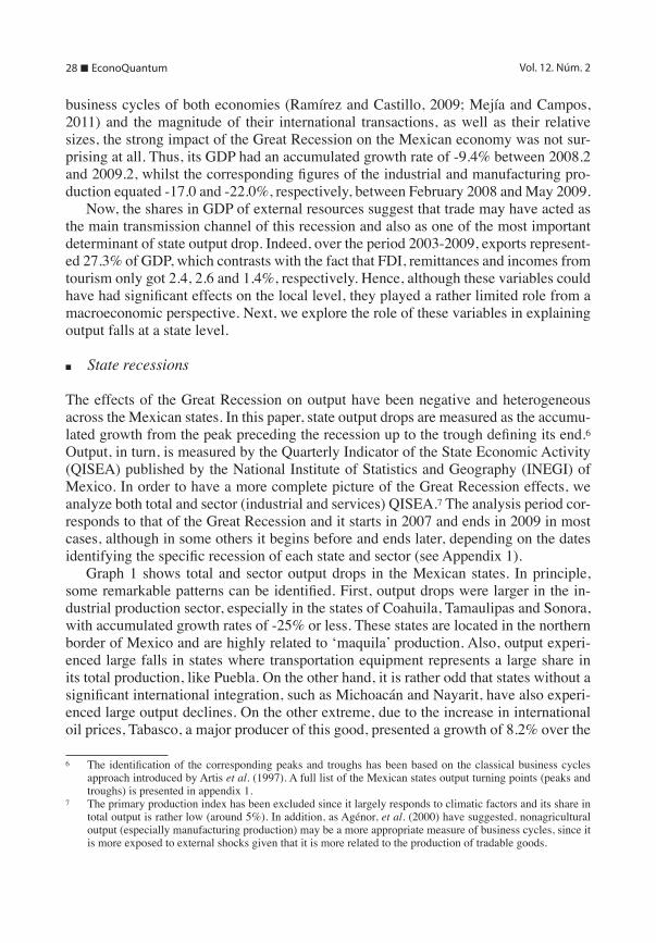
Graph 1 shows total and sector output drops in the Mexican states. In principle, some remarkable patterns can be identified. First, output drops were larger in the in-dustrial production sector, especially in the states of Coahuila, Tamaulipas and Sonora, with accumulated growth rates of -25% or less. These states are located in the northern border of Mexico and are highly related to ‘maquila’ production. Also, output experi-enced large falls in states where transportation equipment represents a large share in its total production, like Puebla. On the other hand, it is rather odd that states without a significant international integration, such as Michoacán and Nayarit, have also experi-enced large output declines. On the other extreme, due to the increase in international oil prices, Tabasco, a major producer of this good, presented a growth of 8.2% over the

6 The identification of the corresponding peaks and troughs has been based on the classical business cycles approach introduced by Artis et al. (1997). A full list of the Mexican states output turning points (peaks and troughs) is presented in appendix 1.

7 The primary production index has been excluded since it largely responds to climatic factors and its share in total output is rather low (around 5%). In addition, as Agénor, et al. (2000) have suggested, nonagricultural output (especially manufacturing production) may be a more appropriate measure of business cycles, since it is more exposed to external shocks given that it is more related to the production of tradable goods.


-32.0 -27.0 -22.0 -17.0 -12.0 -7.0 -2.0 3.0 8.0

AGS

BC

BCS

CAM

COA

COL

CHIA

CHIH

DF

DGO

GTO

GRO

HGO

JAL

MEX

MICH

MOR

NAY

NL

OAX

PUE

QRO

QROO

SLP

SIN

SON

TAB

TAM

TLAX

VER

YUC

ZAC

Services Industrial Total

Graph 1Output drops in Mexican states

Source: Own elaboration based on data from INEGI (2012).


national recession period.8 Second, output of the services sector experienced a gener-alized decline, especially in the case of Quintana Roo, a state specialized in touristic services. Third, the combination of severe falls in output both in the industrial and services sectors yielded considerable falls in total output in most states, especially in Baja California, Tamaulipas, Nuevo León, Colima, Aguascalientes, Querétaro, Puebla, Hidalgo, Guerrero and Chiapas.

The spatial distribution of output drops is presented in Maps 1 to 3. The former shows that falls of industrial production have been larger in the northern bordering states (mainly Sonora, Coahuila and Tamaulipas) and in the center-West region (es-pecially in Jalisco and Nayarit) as well as in some central states that could have been affected by the huge decrease in the industrial output of Puebla. It is worthwhile to underline that accumulated falls of output in this sector range from -2 to -22 per cent in 25 out of 32 states, which indicates a large variability in the performance of industrial output over the Great Recession across the states. Also, it can be seen that six states, located in the central, West-central and northern regions, outstand with accumulated falls that exceeded 21%.

In turn, Map 2 illustrates how the output of the services sector experienced larger drops in the West-central and northern regions. Notice that, in this case, the growth rates ranged from around -12.0% to -5.8%, which suggests that although generalized across the states output falls were more homogeneous within this sector. In principle, these declines in output may be explained by the transmission of external shocks from the manufacturing production to the services sector through activities such as the trans-port, storage, distribution and sales of goods.

Finally, it can be observed in Map 3 that total output drops have been larger in the northern states, which results not surprising given the high degree of integration of their productive processes to those of the US firms. Also, it is interesting to notice that western states exhibited significant drops that may have resulted from the transmission of external shocks from manufacturing to other sectors. We must highlight that the ac-cumulated growth rates of most states in the country lie between -3.0 and -13.0 percent, which clearly indicates the occurrence of generalized deep recessions.

Next, according to the objective of this paper, we explore the existence of (spatial) dependence in the magnitudes of the state output falls. In other words, we analyze the possibility that this variable can be determined not only by factors of the same area, but also by phenomena belongings to neighboring areas. If such is the case, there would be evidence of spatial autocorrelation, which refers to the absence of independence between the observations of a cross-section data set (Anselin, 2005; LeSage and Pace, 2009). More specifically, when locations with high (low) levels of one variable are sur-rounded by locations with also high (low) levels of the same variable it is said that there exists positive spatial autocorrelation. On the contrary, if locations with high (low) levels of one variable are neighbors of locations with low (high) levels of the same variable, then there is evidence of negative spatial autocorrelation.

8 On the basis of the classical business cycle approach, we have dated the peak preceding the national recession in 2008/02 and the subsequent trough in 2009/02.


Map 1Output falls in Mexican states industrial production over the Great Recession



Map 2Output falls in Mexican states services production over the Great Recession


As it is very well known, global spatial autocorrelation can be computed by using the Moran´s I index, which measures the degree of linear association between a vec-tor of observed values and the weighted average of the corresponding values of the neighboring locations for a particular observation. The null hypothesis assessed in this exercise is that there is no spatial autocorrelation and the corresponding test statistic follows a standardized normal distribution (see appendix 2 for details).

The computations of the Moran´s I index yielded the following test statistics (p-values) for total, industrial and services production: -0.297 (0.009), 0.035 (0.279) and -0.056 (0.440), respectively. These results imply that there is evidence of spatial and negative autocorrelation only in the case of total production. Additional evaluation of this property is carried out in the next section in the context of spatial regressions.

n Explaining factors of output drops

The Mexican states output drops experienced during the Great Recession can be ex-plained by multiple factors. On the basis of theoretical models and international em-pirical evidence, aforementioned, and accepting that the recession in Mexico can be seen as a consequence of exogenous demand shocks, the explanatory variables can be organized in three different sets measuring structural exposure to external shocks (ini-tial conditions), specialization in tradable goods, and external demand and fiscal shocks directly linked to the Great Recession.9 9 Notice that the selection of the explanatory variables was also conditioned by data availability.

Map 3Output falls in Mexican states total production over the Great Recession



Hence, the first set relates to the importance in the state economic activity of the international flows of goods and capital that allows us not only measuring the degree of integration of the Mexican states to the global economy, but its sensitivity to external shocks as well. The second set refers to the share in state output of the production of tradable goods, especially of durable goods,10 whose cyclical fluctuations also result to be highly synchronized to the US business cycle. Finally, the third set contains vari-ables associated to the transmission of the Great Recession from the US to the Mexican economy through international transactions as well as to the fiscal policies instrument-ed by the federal and state governments to mitigate its negative effects (Villagómez and Navarro, 2010). Specifically, the model explaining output drops in the Mexican states can be expressed as follows:

(1) y X b X b X b u1 1 2 2 3 3= + + +

where y denotes a n x 1 vector containing the observation of output drops, Xi (for i = 1, 2, 3) denotes a n x ki matrix of explanatory variables, with associated parameters con-tained in the ki x 1 vector bi, and u represents the disturbance vector of order n x 1, with a null vector mean 0 and a variance-covariance matrix v 2I, that is u ~ iidN 0, I2v^ h. The specific variables contained in matrices Xi are as follows: X1 = [REM, X, FDI, TOUR, MAN], X2 = [MAQ, ESPi] and X3 = [TREM, TFDI, TGi], where REM, X, FDI, TOUR and MAN denote the share in state GDP of remittances, exports, foreign direct invest-ment, tourism and manufacturing production; notice that exports are also measured as the share of the basic sector in GDP (BAS).11 MAQ stands for the ratio of ‘maquila’ to manufacturing production, while ESPi denotes different specialization variables such as the share in manufacturing production of the transportation equipment production (AUT), as well as different combinations of the production of textiles (sector 2), chemi-cals (sector 5) and metallic products and machinery and equipment (sector 8), denoted as R258, R28 and R58. 12 In matrix X3, the prefix “T” denotes the growth rate of the cor-responding variable. Finally, Gi denotes government expenditure, as measured by the net federal expenditure (NFE), net state expenditure (NSE) and federal fix investment by state (FFIS). Further details of the data set are given in appendix 3.

10 Tradable goods experienced large falls in international trade over the Great Recession, especially durable goods, such as automobiles (Bems, et al., 2010). In Mexico, manufactured goods represent 82.6% in total exports, while the share in exported manufactured goods of metallic products, machinery and equipment gets 73.8%. In turn, transportation equipment represents 36.2% in the latter, according to information of INEGI.

11 The basic sector refers to the production of tradable goods and includes: agriculture, livestock, forestry, fishing, hunting, mining, manufacturing, temporary accommodation and preparation of food and beverage services. On the other hand, notice that there is not official information of international trade at state level. Therefore, state exports of 2007 are just estimates that may suffer of the “fiscal address bias”, which refers to the fact that the place of origin of exports is related to the fiscal address of the firm rather than to the actual production location. Similar limitations are present in the data of FDI.

12 These activities are highly correlated to the US business cycle as a consequence of the participation of inter-national firms, which are linked to foreign direct investment and carry out a large proportion of total interna-tional trade (see Mejía et al., 2006a).


Now, eight different specification models are defined depending of the use of al-ternative variables to measure exports and specialization. The first four specifications include X whilst the latter do so with BAS. In turn, AUT, R28, R58 and R258 define four models in each case giving a total of eight.

In addition, model (1) has been extended in order to incorporate the effects of space in the dynamics of output drops. On the basis of the corresponding statistic tests (pre-sented below), spatial autoregressive models are the most appropriated.13 Then, for-mally, the general model can be specified as:

(2) y Wy X b X b X b u1 1 2 2 3 3t= + + + +

where W is the row-standardized spatial weight matrix with entries equal to 1 if the states share a border and 0 otherwise; therefore, Wy is the spatial lag of the endogenous variable, t is the spatial autoregressive coefficient which reflects the intensity of in-terdependencies between the sample observations, and u is the random variable that follows a white noise process.

n Estimation and results

Model (2) is used to explain output drops in the Mexican states as a function of the explanatory variables defined in expression (1). Then, following Anselin (2005), this model has been chosen on the basis of the Lagrange multiplier (LM) tests defined in appendix 2. The estimated p-values of the statistics LM(lag) and LM(error) to evalu-ate the null of no spatial autocorrelation between the dependent variable (substantive autocorrelation) and the residuals (residual autocorrelation) in the regression model (1), estimated by ordinary least squares, are presented in Table 1. The set of statistic tests also includes versions robust to misspecifications, which are denoted as RLM(lag) and RLM(error), respectively.

In the case of total QISEA, the estimated p-values of the LM(lag) test statistic al-low us to reject the null at least at 5% of significance for all specifications, while the estimates corresponding to the LM(error) statistic allow us to do so only at 10% in the case of specifications 4, 5 and 8. However, since the estimated p-values of the LM(lag) statistics are lower than those of the RLM(error) statistics, we decided to estimate lag regression models for the whole set of specifications.14 In turn, notice that the estimated LM test statistics provide support to the null hypothesis of no autocorrelation for all model specifications in the cases of industrial and services QISEA. Altogether, this evi-dence is consistent with that provided by the Moran´s I index. Thus, there seems to be spatial autocorrelation only in the case of total QISEA. Consequently, the econometric analysis is based on model (2) for total QISEA and model (1) for industrial and services

13 Spatial error regression models are not reported since there is no evidence supporting their use in explaining output drops in the Mexican states (see below).

14 This conclusion is also supported by the robust versions of the LM tests. However, error regression models were also estimated, but the autocorrelation coefficients were not statistically significant.


Table 1p values of the LM tests to choose between lag or spatial error models

Source: Own elaboration.

Modelos 1 2 3 4 5 6 7 8

Total QUISEA LM (lag) 0.014 0.004 0.027 0.002 0.003 0.002 0.008 0.001 RLM (lag) 0.022 0.001 0.004 0.006 0.011 0.000 0.001 0.001 LM (error) 0.145 0.241 0.495 0.073 0.086 0.253 0.475 0.096 RLM (error) 0.261 0.068 0.052 0.303 0.344 0.037 0.041 0.166

Industrial QUISEA

LM (lag) 0.959 0.665 0.685 0.707 0.861 0.395 0.400 0.456 RLM (lag) 0.432 0.959 0.667 0.587 0.405 0.951 0.939 0.391 LM (error) 0.578 0.627 0.843 0.413 0.486 0.309 0.352 0.169 RLM (error) 0.337 0.820 0.807 0.364 0.284 0.575 0.687 0.150

Services QUISEA

LM (lag) 0.465 0.406 0.512 0.551 0.500 0.425 0.497 0.551 RLM (lag) 0.262 0.212 0.223 0.248 0.265 0.208 0.231 0.299 LM (error) 0.855 0.849 0.995 0.990 0.906 0.895 0.980 0.955 RLM (error) 0.384 0.341 0.305 0.323 0.370 0.325 0.324 0.394

QISEA. The final specification of each model was obtained following a “general to specific approach”: essentially, models defined in (1) and (2) are estimated and then the least significant variable is dropped out and the model is estimated again. The process continues up to the point when all variables are statistically significant at least at a 10% level of significance.

The results for the industrial and services production are shown in Tables 2 and 3. As it can be seen, the estimated models explain over 55% of the output drops variabil-ity, as measured by the determination coefficient R2.15 It is worth underlining that the estimates of the parameters are largely robust both in terms of value and sign. In gen-eral, the exposure variables have the negative expected sign suggesting that the higher the exposition to external shocks the greater the fall in output.

More specifically, regarding the exposure variables in the case of industrial produc-tion, the shares in state GDP of exports (X), remittances (REM) and tourism (TOUR) have negative and statistically significant effects on output drops, as suggested by the literature. In turn, among the specialization variables, when X enters into the model, only the share of transportation equipment in manufacturing production (AUT) is sig-nificant and has a negative impact on output drops. In contrast, if the ratio of the basic sector is used as a proxy of international trade (BAS, which is not significant), AUT, 15 There is no specification problems associated to non-normality and heteroskedasticity.


Table 2Estimation results for the industrial sector (estimation by OLS)

Numbers in parenthesis are t statistics. Figures reported for specification tests are p-values.Source: Own elaboration.

Model 1 2 3 4 5 6 7 8

X --- -0.28 -0.28 -0.28

--- --- --- --- (-2.65) (-2.65) (-2.65)

REM

-1.06 -0.99 -0.99 -0.99 -1.06 ---

-1.17 ---

(-2.92) (-1.80) (-1.80) (-1.80) (-2.92) (-2.93)

TOUR

-0.56 -0.86 -0.86 -0.86 -0.56 ---

-0.65 ---

(-2.05) (-2.99) (-2.99) (-2.99) (-2.05) (-2.02)

MAN --- --- --- --- --- --- ---

0.65 (2.77)

AUT

-0.21 --- --- ---

-0.21 --- --- ---

(-3.08) (-3.08)

R28 --- --- --- --- --- ---

-0.26 ---

(-2.10)

R58 --- --- --- --- --- --- ---

-0.34 (-2.01)

NFE ---

-1.29 -1.29 -1.29 --- --- --- ---

(-2.18) (-2.18) (-2.18)

NSE --- --- --- --- ---

-1.16 ---

-1.64 (-2.52) (-2.12)

FPIS ---

5.44 5.44 5.44 3.29 ---

5.91 (3.09) (3.09) (3.09) (1.82) (2.23)

TREM

-0.78 --- --- ---

-0.78 -0.72 -0.72 ---

(-3.77) (-3.77) (-3.06) (-3.18)

TBAS

0.92 0.94 0.94 0.94 0.92 1.01 0.96 1.46 (3.01) (2.49) (2.49) (2.49) (3.01) (2.72) (2.82) (3.47)

TNSE

-0.54 -0.72 -0.72 -0.72 -0.54 -0.61 -0.53 -0.63 (-3.43) (-3.58) (-3.58) (-3.58) (-3.43) (-3.09) (-3.12) (-3.25)

TFPIS --- --- --- --- --- --- ---

0.05 (2.28)

R2 0.68 0.62 0.62 0.62 0.68 0.56 0.63 0.61

Normality 0.84 0.34 0.34 0.34 0.86 0.88 0.42 0.57

Heteroskedasticity 0.81 0.92 0.92 0.92 0.81 0.75 0.90 0.94


Table 3Estimation results for the services sector (estimation by OLS)

Model 1 2 3 4 5 6 7 8

TOUR -0.33 -0.33 -0.35 -0.33 -0.33 -0.33 -0.33 -0.33(-4.50) (-4.50) (-4.57) (-4.50) (-4.50) (-4.50) (-4.50) (-4.50)

MAN -0.06 -0.06 -0.08 -0.06 -0.06 -0.06 -0.06 -0.06(-2.17) (-2.17) (-2.32) (-2.17) (-2.17) (-2.17) (-2.17) (-2.17)

MAQ -0.02 -0.02 -0.02 -0.02 -0.02 -0.02 -0.02 -0.02(-2.20) (-2.20) (-2.20) (-2.20) (-2.20) (-2.20) (-2.20) (-2.20)

NFE 0.17 0.17 0.21 0.17 0.17 0.17 0.17 0.17(2.74) (2.74) (2.74) (2.74) (2.74) (2.74) (2.74) (2.74)

TBAS --- --- -0.09 --- --- --- --- ---(-0.93)

R2 0.59 0.59 0.60 0.59 0.59 0.59 0.59 0.59Normality

0.34 0.34 0.31 0.34 0.34 0.34 0.34 0.34Heteroskedasticity 0.89 0.89 0.82 0.89 0.89 0.89 0.89 0.89


R28 and R58 have separated statistically significant and negative effects on output, such as the theory suggests. On the other hand, among the direct effects of the Great Recession, only the growth rate of the basic sector (TBAS) has statistically significant and positive effects on output drops, which suggest that negative external shocks asso-ciated to the Great Recession had actually adverse impacts on state production. In addi-tion, there seems to be evidence of a counter-cyclical fiscal policy implemented by the states given that the estimated coefficient of the growth rate of the net state expenditure (TNSE) is negative and significant. On the contrary, the estimation results suggest that the federal fiscal policy has been ineffective and insufficient since the coefficient of the growth rate of federal physical investment in states is statistically significant only in one specification and its sign is positive, implying that the policy was pro-cyclical; this result, however, is not robust. 16

16 A couple of odd results deserve some comments. First, the ratio of manufacturing production to GDP is sig-nificant only in specification 8 and has a positive coefficient. A possible explanation of this result is that total manufacturing production is not the relevant variable to measure external exposure or productive processes integration but its composition, since specific activities have statistically significant effects. Second, the nega-tive effects of the growth rate of remittances suggest that this variable has not been an important determinant of state output dynamics, since its large falls seem to be associated to small drops in state production; this


On the other hand, the output drops in the services sector are explained by a small set of variables, as seen in Table 3.17 In general, the estimated models explain nearly 60% of output drops variability. The specific variable that seems to be the most impor-tant in the explanation of the tertiary output drops is the ratio of the tourism sector out-put to state GDP (TOUR), since its estimated coefficient is the greatest one in absolute terms and is statistically significant, which is a quite reasonable result since tourism activities are related to the supply of the most tradable goods and services within this sector. Other variables having negative and significant effects, although their estimated coefficients are small, are the share of manufacturing production in state GDP and the share of “maquila” production in state manufacturing production. To interpret this re-sult, it can be hypothesized that greater exposure in the manufacturing and “maquila” production causes larger output drops that spills over through falls in local employment and income, provoking falls in lower local demand of largely non-tradable goods sup-plied by the tertiary sector. In turn, among fiscal variables only the net federal expendi-ture (NFE) has positive and significant effects, a result that is greatly robust, implying that federal fiscal policy has actually been pro-cyclical. Notice that all initial model specifications converge to the same one at the end.

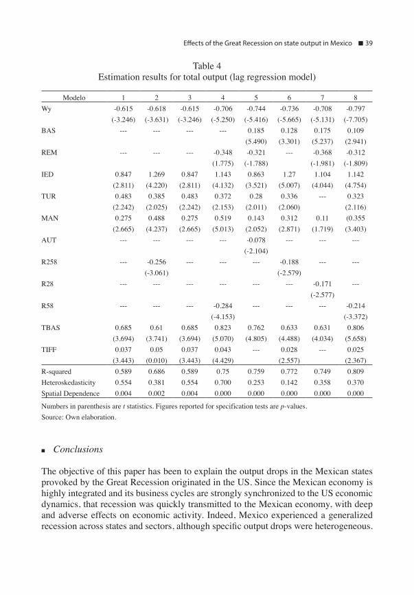
Finally, total output drops are explained by a wider set of variables; the results are reported in Table 4. Consistent with the results yielded by the Moran’s I index, the autoregressive coefficient is negative and statistically significant, suggesting that states with large output drops are neighbors of states with small drops, such as it can be seen in Map 3. The explanatory power of the estimated models varies from 59 to 81% ac-cording to the determination coefficients.18 Regarding the explanatory variables, sever-al interesting aspects can be identified. First, most exposure variables have positive and statistically significant coefficients, which is rather odd. A possible explanation may be related to the relatively small size of the ratios IED, TOUR, MAN and BAS as well as to the nature of productive activities, which are largely linked to non-tradable goods and services in many states.19 Second, higher specialization in the production of transpor-tation equipment and, especially, of chemicals and metallic products, machinery and equipment (R25), implies deeper state recessions, as suggested by the literature. Final-ly, it seems that state government expenditure played no role to mitigate the effects of the Great Recession on the performance of total output, whilst the federal government expenditure contributed to deepen the global recession effects through significant cuts in federal fix investment by state (TFFIS), as indicated by its positive and statistically significant coefficient.

seems to be a sensible interpretation given their relatively low share in state GDP. 17 There is no evidence of non-normality and heteroskedasticity in the residuals.18 There is no evidence of heteroskedasticity, although the null of no spatial autocorrelation in the residuals

is rejected despite lagged values of the endogenous variable are considered in this framework. Alternative second-order autocorrelation models were also estimated, but the problem remained.

19 Another possibility to be explored in the future is related to the existence of outliers that may be distorting the estimates.


Table 4Estimation results for total output (lag regression model)

Modelo 1 2 3 4 5 6 7 8Wy -0.615 -0.618 -0.615 -0.706 -0.744 -0.736 -0.708 -0.797

(-3.246) (-3.631) (-3.246) (-5.250) (-5.416) (-5.665) (-5.131) (-7.705)BAS --- --- --- --- 0.185 0.128 0.175 0.109

(5.490) (3.301) (5.237) (2.941)REM --- --- --- -0.348 -0.321 --- -0.368 -0.312

(1.775) (-1.788) (-1.981) (-1.809)IED 0.847 1.269 0.847 1.143 0.863 1.27 1.104 1.142

(2.811) (4.220) (2.811) (4.132) (3.521) (5.007) (4.044) (4.754)TUR 0.483 0.385 0.483 0.372 0.28 0.336 --- 0.323

(2.242) (2.025) (2.242) (2.153) (2.011) (2.060) (2.116)MAN 0.275 0.488 0.275 0.519 0.143 0.312 0.11 (0.355

(2.665) (4.237) (2.665) (5.013) (2.052) (2.871) (1.719) (3.403)AUT --- --- --- --- -0.078 --- --- ---

(-2.104)R258 --- -0.256 --- --- --- -0.188 --- ---

(-3.061) (-2.579)R28 --- --- --- --- --- --- -0.171 ---

(-2.577)R58 --- --- --- -0.284 --- --- --- -0.214

(-4.153) (-3.372)TBAS 0.685 0.61 0.685 0.823 0.762 0.633 0.631 0.806

(3.694) (3.741) (3.694) (5.070) (4.805) (4.488) (4.034) (5.658)TIFF 0.037 0.05 0.037 0.043 --- 0.028 --- 0.025

(3.443) (0.010) (3.443) (4.429) (2.557) (2.367)R-squared 0.589 0.686 0.589 0.75 0.759 0.772 0.749 0.809Heteroskedasticity 0.554 0.381 0.554 0.700 0.253 0.142 0.358 0.370Spatial Dependence 0.004 0.002 0.004 0.000 0.000 0.000 0.000 0.000


n Conclusions

The objective of this paper has been to explain the output drops in the Mexican states provoked by the Great Recession originated in the US. Since the Mexican economy is highly integrated and its business cycles are strongly synchronized to the US economic dynamics, that recession was quickly transmitted to the Mexican economy, with deep and adverse effects on economic activity. Indeed, Mexico experienced a generalized recession across states and sectors, although specific output drops were heterogeneous.


In this paper, quarterly indexes of total, industrial and services production of the Mexican states are analyzed. Spatial (to give account of the recession transmission from one state to another) or cross-sectional regression models have been formulated and estimated to explain differences in the state output drops. However, the specifica-tion tests, such as the Moran’s I index and the Lagrange multiplier tests, suggest that spatial autocorrelation is present only in the case of total production.

The explanatory variables were divided in three different sets: measures of expo-sure to external shocks, specialization patterns and external demand and fiscal shocks. In general, exposure variables were relevant to explain sectorial output drops, but not total declines in production. In particular, industrial output falls can be explained by the share in state GDP of exports, remittances and tourism, while the shares in state GDP of tourism and manufacturing have played an important role in the explanation of reces-sions in the services sector. The estimated coefficients of most of these variables are negative suggesting that the higher the exposure to external shocks, the larger the state output drops. The specialization variables have also had negative impacts on output implying that the higher the specialization of the state economy in the production of tradable goods (mainly durable goods), the larger the drops in output.

On the other hand, total production shows evidence of negative and significant spa-tial autocorrelation, which does not support the hypothesis of transmission of the reces-sion from one state to its neighbors. On the contrary, this evidence indicates that states with deep recessions have neighbors with small output drops and vice versa. Regarding the explanatory variables, the results suggest that the specialization in the production of transportation equipment and chemicals and metallic products, machinery and equip-ment provoked larger drops in total output. In addition, the direct adverse effects of the Great Recession, as measured by the negative growth rate of the basic sector, but not the structural exposure to external shocks, played a significant role in the reduction of the state total production.

Finally, the estimation results suggest that the federal fiscal policies played no role or even amplified the adverse effects of the Great Recession at state level, especially in the case of the total and services production. On the contrary, state government expen-diture contributed to mitigate the effects of the recession in the industrial sector only. Overall this evidence reflects a limited or counterproductive performance of the federal and state governments in the stabilization of the effects of the past recession. Neverthe-less, looking ahead, it is worth wondering whether this is the best role the governments should play in the context of more open local economies.


n Appendix 1

Appendix 1Turning points of total and sector production

States Total Industrial Services Peak Trough Peak Trough Peak Trough

AGS 2008/02 2009/01 2008/02 2009/01 2008/03 2008/04BC 2008/02 2009/02 2008/02 2009/02 2008/01 2009/02BCS 2008/02 2009/02 2009/02 2010/02 2010/01 2010/02CAM 2008/02 2009/02 2008/02 2009/02 2008/04 2009/01CHIA 2008/03 2009/02 2008/03 2009/03 2008/04 2009/01CHIHU 2008/01 2009/01 2008/02 2010/04 2008/04 2009/01COAUH 2008/02 2009/02 2007/03 2009/02 2008/03 2009/02COL 2008/02 2009/02 2007/03 2009/02 2008/01 2009/02DF 2008/02 2009/02 2007/03 2009/01 2008/02 2009/02DGO 2008/02 2009/01 2008/01 2009/01 2008/03 2009/02GRO 2008/02 2009/02 2008/02 2009/02 2008/01 2009/02GTO 2007/03 2009/02 2006/01 2009/02 2008/02 2009/02HGO 2008/03 2009/02 2009/02 2010/01 2008/02 2009/02JAL 2008/02 2009/02 2007/01 2009/02 2008/02 2009/02MEX 2008/02 2009/02 2008/02 2009/02 2008/02 2009/02MICH 2008/02 2009/02 2008/02 2009/01 2008/03 2009/02MOR 2008/02 2009/02 2007/02 2008/04 2008/01 2009/02NAY 2009/02 2011/04 2008/03 2009/03 2008/03 2009/02NL 2008/02 2009/02 2008/02 2009/01 2008/02 2009/02OAX 2009/02 2011/04 2005/04 2010/01 2008/03 2009/02PUE 2008/02 2009/02 2008/02 2009/02 2008/02 2009/02QRO 2008/01 2009/02 2008/01 2009/01 2008/01 2009/02QROO 2008/02 2009/04 2008/02 2009/02 2008/03 2009/02SIN 2008/02 2009/02 2008/04 2009/03 2008/02 2009/02SLP 2008/02 2009/02 2008/02 2009/01 2008/02 2009/02SON 2008/02 2009/02 2006/04 2009/01 2008/02 2009/02TAB 2008/02 2009/02 2008/02 2009/02 2008/03 2009/02TAM 2008/01 2009/03 2008/01 2009/03 2008/02 2009/02TLAX 2008/03 2009/02 2006/02 2009/04 2008/02 2009/02VER 2007/04 2009/02 2007/04 2008/03 2008/02 2009/02YUC 2008/01 2009/01 2007/02 2008/04 2008/02 2009/02ZAC 2008/02 2009/02 2009/02 2009/04 2008/03 2009/02



n Appendix 2. Moran’s I Index and spatial autocorrelation LM tests

The Moran’s I index

It is a univariate test statistic that evaluates the null hypothesis of no autocorrelation. Conventionally, it is formulated as,

(A1) I

SN

y y

w y y yy2

iN

i

ij i j

0 12R

R=

-

- -

= ^^ ^^

hh hh

where ,S w wi j ij ij0 2R R R= = ^ h i.e., the sum of spatial weights; y is the mean or expected value of the variable y and N is the number of observations or sample size. Asymptoti-cally, it follows a standard normal function, N(0,1).

Spatial autocorrelation LM tests

Based on the principle of Lagrange multipliers, the LM(error) test is expressed in its matrix form as:

(A2) ( )LM error

Tse We

1

2

2

=

l; E

where W represents the spatial weight matrix, e is the OLS estimation residual vector,

s e eN

2 = l and T tr W W W12= +l6 @. This test has a null hypothesis no spatial residual

autocorrelation. The RLM(error) test is an adjusted version, robust to local misspecification. Its for-

mal expression would be the following:

(A3) ( )( )

1

RLM errorT T RJ

se We T RJ

s

e Wy2 1 2

1 12

2

=-

--

t b

t b

-

-

l l

u

u

^ h; E

where RJ TS

WX M WX1

1 2

1b b= +t b-

-

-lu^ ^ ^h h h; E , WXb is a spatial lag of the predicted

values from an OLS regression of (1), M I X X X X1= - -l l^ h is the familiar projection matrix.

On the other hand, the LM(lag) test is used to evaluate the null hypothesis of no autocorrelation in the endogenous variable. Its formal expression is:


(A4) LM LAG

RJ

s

e Wy2

2

- =t b-

l

u

; E

An alternative test, robust to the presence of local dependence of a spatial error, is the RLM(lag) test, which can be expressed as,

(A5) LM EL

RJ T

s

e W y

se W e

2

1

21

1

2

- =-

-

t b-

l l

u

; E

n Appendix 3. Variable definitions and data sources

Nomenclature Variable Original units Sample period SourcesGDP Gross Domestic Product Millions of dollars 2003-2007

(annual)INEGI

TOUR Ratio of Tourism services* to GDP.

Millions of dollars 2003-2007 (annual)

INEGI

REM Ratio of Remittances to GDP. Millions of dollars 2003-2007 (annual)

INEGI

FDI Ratio of Foreign Direct Investment to GDP.

Millions of dollars 2003-2007 (annual)

INEGI

X Ratio of Exports to GDP. Millions of dollars 2007 AregionalMAN Ratio of Manufacturing

production to GDP.Thousands of pesos 1993

2003-2006 INEGI

MAQ Ratio of “Maquila” to Manufacturing production.

Millions of pesos 1993

2003-2006 (annual)

INEGI

AUT Ratio of Transportation equipment production to Manufacturing production.

Thousands of pesos 2008 INEGI. Censos Económicos

BAS Ratio of Basic Sector ** to GDP. Thousands of pesos 2003-2007 INEGINFE Net federal expenditure Thousands of pesos 2003-2007 INEGI. Finanzas Públicas

Estatales y MunicipalesNSE Net state expenditure Thousands of pesos 2003-2007 INEGI. Finanzas Públicas

Estatales y MunicipalesFPIS Federal physical investment by

state.Constant pesos 2003

2003-2007 SHCP. Unidad de Coordinación con Entidades Federativas.

TREM Growth Rate of Remittances Percentages 2008-2009 INEGI


Nomenclature Variable Original units Sample period SourcesTFDI Growth Rate of Foreign Direct

InvestmentPercentages 2008-2009 INEGI

TBAS Growth Rate of the Basic sector Percentages 2008-2009 INEGITNFE Growth Rate of Net federal

expenditurePercentages 2008-2009 INEGI. Finanzas Públicas

Estatales y MunicipalesTNSE Growth Rate of Net state

expenditurePercentages 2008-2009 INEGI. Finanzas Públicas

Estatales y MunicipalesTFPIS Growth rate of Federal physical

investment by state Percentages 2008-2009 SHCP. Unidad de

Coordinación con Entidades Federativas.

*Tourism services include temporary accommodation and preparation of food and beverage services.** The basic sector includes agriculture, livestock, forestry, fishing, hunting, mining, manufacturing, temporary accommodation and preparation of food and beverage services. Source: Own elaboration.

n References

Agénor, P. R., McDermott, C. J. and Prasad, E. S. (2000). “Macroeconomic fluctuations in developing countries: some stylised facts”. World Bank Economic Review, 14 (2): 251-285.

Anselin, L. (2005). Exploring spatial data with GeoDaTM: A workbook. Department of Geography. University of Illinois: 1-224.

Aregional (2012). Información para decidir. Available online: http://www.aregional.com/

Artis, M. J., Kontolemis, Z. G. and Osborn, D. R. (1997). “Business Cycles for G7 and European Countries”. The Journal of Business, 70 (2): 249-279.

Bems, R., Johnson, R. C. and Yi, K. - M. (2010). “Demand spillovers and the collapse of trade in the global recession”. IMF Economic Review, 58, 295-326.

Berkmen, P., Gelos, G., Rennhack, R. and Walsh, J. P. (2009). “The global financial cri-sis: explaining cross-country differences in the output impact”. IMF Working Paper WP/09/280: 2-19.

Blanchard, O. (2009). “The crisis: basic mechanisms, and appropriate polices”. IMF Working Paper WP/09/80: 3-22.

Blanchard, O., Das, M. and Faruqee, H. (2010). “The initial impact of the crisis on emerg-ing market countries”. Brookings Papers on Economic Activity, 41 (1): 263-323.

Castillo, R., Díaz, A. and Fragoso, E. (2004). “Sincronización entre las economías de México y Estados Unidos: el caso del sector manufacturero”. Comercio Exterior, 54 (7): 620-627.

Chiquiar, D. and Ramos, M. (2005). “Trade and Business-Cycle Synchronization: Evi-dence from Mexican and U.S. Manufacturing Industries”. North American Journal of Economics and Finance, 16 (2): 187-216.


Gutiérrez, E. E., Mejía, P. and Cruz, B. (2005). “Ciclos económicos y sector externo en México. Evidencia de relaciones cambiantes en el tiempo”. Estudios Económicos de Desarrollo Internacional, 5 (1): 65-92.

Herrera, J. (2004). “Business cycles in Mexico and the United States: do they share common movements?” Journal of Applied Economics, VII (2): 303-323.

INEGI (2012). Banco de Información Económica. México. Available online: http://www.inegi.org.mx/sistemas/bie/?idserPadre=10000330

Imbs, J. (2010). “The first global recession in decades”. IMF Economic Review, 58, 327-354.

IMF (2009). “World Economic Outlook: Crisis and Recovery”. International Monetary Fund, 1-60.

LeSage, J. and Pace, R. K. (2009). Introduction to spatial econometrics. Boca Raton, CRC Press: 20-28.

Levchenko, A. A., Lewis, L. T. and Tesar, L. L. (2010). “The collapse of international trade during the 2008-2009 crisis: in search of the smoking gun”. NBER Working Paper, 16006: 1-54.

Llaudes, R., Salman, F. and Chivakul, M. (2010). “The Impact of the Great Recession on Emerging Markets”. IMF Working Paper, WP/10/237: 2-34.

Mejía, P., Gutiérrez, E. E. and Farías, C. A. (2006a). “La sincronización de los ciclos económicos de México y Estados Unidos”. Investigación Económica, 45 (258): 15-45.

Mejía, P., Gutiérrez, E. E. and Pérez, J. A. (2006b). “Los claroscuros de la sincroni-zación internacional de los ciclos económicos: evidencia sobre la manufactura de México”. Ciencia Ergo Sum, 13 (2): 133-142.

Mejía, P. and Campos, J. (2011). “Are the Mexican States and the United States Business Cycles Synchronized? Evidence from the Manufacturing Production”. Economía Mexicana. Nueva Época, XX (1): 79-112.

Moreno-Brid, J. C. and Ros, J. (2009). Development and Growth in the Mexican Econ-omy. Oxford, Oxford University Press: 1.328

Ponce, A. (2001). “Determinantes de los ciclos económicos en México: ¿Choques agregados o desagregados?” Gaceta de Economía, 6 (12): 117-154.

Ramírez, R. and Castillo, R. A. (2009). “Integración económica en América del Norte: lección de la experiencia de la Unión Europea para el TLCAN”. Estudios Fronter-izos, 10 (19): 183-208.

SHCP (2012). Coordinación con entidades federativas. Available online: http://www.shcp.gob.mx/POLITICAFINANCIERA/FINANZASPUBLICAS/Estadisticas_Oportunas_Finanzas_Publicas/Informacion_mensual/Paginas/coordinacion.aspx

Villagómez, A. and Navarro, L. (2010). Política fiscal contracíclica en México durante la crisis reciente: un análisis preliminar. CIDE Documento de Trabajo 475: 1-31.

Wang, J. (2010). “Durable goods and the collapse of global trade”. Economic Letter, 5 (2): 1-8.

Effects of the Great Recession on state output in Mexico

Documents

Transcript of Effects of the Great Recession on state output in Mexico