
EFFECTS OF NEAR-FAULT GROUND MOTIONS ON FRAME STRUCTURES
311
Department of Civil and Environmental Engineering Stanford University EFFECTS OF NEAR-FAULT GROUND MOTIONS ON FRAME STRUCTURES by Babak Alavi and Helmut Krawinkler Report No. 138 February 2001
Transcript of EFFECTS OF NEAR-FAULT GROUND MOTIONS ON FRAME STRUCTURES
Department of Civil and Environmental Engineering
Stanford University
EFFECTS OF NEAR-FAULT GROUND MOTIONS ON FRAME STRUCTURES
by
Babak Alavi
and
Helmut Krawinkler
Report No. 138
February 2001
The John A. Blume Earthquake Engineering Center was established to promote research and education in earthquake engineering. Through its activities our understanding of earthquakes and their effects on mankind’s facilities and structures is improving. The Center conducts research, provides instruction, publishes reports and articles, conducts seminar and conferences, and provides financial support for students. The Center is named for Dr. John A. Blume, a well-known consulting engineer and Stanford alumnus. Address: The John A. Blume Earthquake Engineering Center Department of Civil and Environmental Engineering Stanford University Stanford CA 94305-4020 (650) 723-4150 (650) 725-9755 (fax) earthquake @ce. stanford.edu http://blume.stanford.edu
©2001 The John A. Blume Earthquake Engineering Center
EFFECTS OF NEAR-FAULT GROUND MOTIONS ON FRAME STRUCTURES
by Babak Alavi
and Helmut Krawinkler
The John A. Blume Earthquake Engineering Center Department of Civil and Environmental Engineering
Stanford University Stanford, CA 94305-4020
A report on research sponsored by
CUREe-Kajima Phase III National Science Foundation Grant CMS-9812478
California SMIP Contract No. 1097-601
Report No. 138
February 2001

Abstract i
ABSTRACT
Near-fault ground motions have caused much damage in the vicinity of seismic sources during recent earthquakes. These ground motions come in large varieties and impose high demands on structures compared to “ordinary” ground motions. Recordings suggest that near-fault ground motions are characterized by a large high-energy pulse. This impulsive motion, which is particular to the “forward” direction, is mostly oriented in a direction perpendicular to the fault, causing the fault-normal component of the motion to be more severe than the fault-parallel component. This study is intended to evaluate and quantify salient response attributes of near-fault ground motions and to investigate design guidelines that explicitly account for near-fault effects. In this study the elastic and inelastic response of SDOF (single degree of freedom) systems and MDOF (multi degree of freedom) frame structures to near-fault and pulse-type ground motions is investigated. Generic frame models are utilized to represent MDOF structures. The stiffness and strength of the models are tuned to a story shear distribution based on the SRSS (square root of sum of squares) combination of modal responses. The extent to which these models represent code-compliant structures is evaluated by comparing the dynamic response of the generic frames with that of steel structure models. Near-fault ground motions are represented by equivalent pulses, which have a comparable effect on structural response but whose characteristics are defined by a small number of parameters. The inelastic dynamic response to both near-fault records and basic pulses demonstrates that structures with a fundamental period greater than the pulse period respond differently than shorter period structures. For the former, early yielding occurs in higher stories but the high ductility demands migrate to the bottom stories as the ground motion becomes stronger. For the latter, the maximum demand always occurs in the bottom stories.

Abstract ii
Models are proposed that relate the parameters of the equivalent pulse to magnitude and distance by means of regression analysis. A preliminary design methodology is developed based on the equivalent pulse concept, including a procedure that provides an estimate of the base shear strength required to limit story ductility ratios to specific target values. Alternative story shear strength distributions are introduced that can improve the distribution of ductility demands over the height for long period frames. Strengthening of frames with walls that are either fixed or hinged at the base is studied, and it is shown that strengthening with hinged walls can provide effective protection against near-fault effects at all performance levels.
Acknowledgements iii
ACKNOWLEDGEMENTS
This report is a reproduction of the senior author’s Ph.D. dissertation. The dissertation is the result of an extensive study on the effects of near-fault ground motions on frame structures. This study has been supported by a grant from the CUREe/Kajima Research Program, by the National Science Foundation through Grant CMS-9812478 of the US-Japan Cooperative Research Program in Urban Hazard Mitigation, and by the California Department of Conservation as a SMIP 1997 Data Interpretation Project (Department of Conservation Contract No. 1097-601). This support is gratefully acknowledged. The constructive collaboration of Dr. Paul Somerville on the ground motion aspects of this research is much appreciated. The authors express their appreciation to Professors Allin Cornell, Eduardo Miranda, and Greg Deierlein, who provided constructive feedback on the manuscript. Several researchers of the John A. Blume Earthquake Engineering Center have contributed to this work. Sincere thanks are due to all of them, especially to Nicolas Luco for his collaboration and constructive feedback, and to Dr. Hjortur Thrainsson for sharing his extensive knowledge of earthquake engineering with the senior author.
Table of Contents iv
TABLE OF CONTENTS
Chapter 1. Introduction 1.1. Statement of Problem ....................................................................................... 1 1.2. Historical Perspective ....................................................................................... 3 1.3. Objectives and Scope ....................................................................................... 4 Chapter 2. Near-Fault Ground Motions Used in this Study 2.1. Ground Motion Records ................................................................................... 8 2.1.1. Directivity Effects ............................................................................. 9 2.1.2. Ground Motion Components ........................................................... 10 2.2. Elastic Spectra of Near-Fault Ground Motions .............................................. 10 2.2.1. Comparison with Ordinary Ground Motions .................................. 12 Chapter 3. SDOF and MDOF Systems Used in this Study 3.1. SDOF Systems ............................................................................................... 23 3.2. MDOF Systems .............................................................................................. 23 3.2.1. Properties of Generic Structure ....................................................... 23 3.2.2. Design Load Pattern ........................................................................ 25 3.2.3. P-Delta Effects ................................................................................ 26 Chapter 4. Response of Structures to Near-Fault Ground Motions 4.1. Elastic Response of MDOF Structures ........................................................... 31 4.1.1. Elastic Base Shear Demands ........................................................... 31 4.1.2. Elastic Shear Force Distribution Over Height of Structure ............. 32 4.1.3. Elastic Roof Displacement Demands .............................................. 33 4.2. Ductility Demands for Inelastic Structures .................................................... 34 4.2.1. SDOF Systems ................................................................................ 34

Table of Contents v
4.2.2. MDOF Systems ............................................................................... 37 4.3. Displacement Demands for Inelastic Structures ............................................ 42 4.3.1. SDOF Inelastic Displacement Demands ......................................... 42 4.3.2. MDOF Inelastic Roof Displacement Demands ............................... 43 Chapter 5. Pulse-Type Seismic Input 5.1. Historical Perspective ..................................................................................... 68 5.2. Basic Pulse Shapes Used in this Study ........................................................... 69 5.2.1. Elastic Response Spectra ................................................................. 71 5.3. Other Pulse Shapes ......................................................................................... 72 5.3.1. Triangular Pulses ............................................................................. 72 5.3.2. Pulse Histories with Different Duration .......................................... 73 Chapter 6. Response of Structures to Pulse-Type Seismic Input 6.1. Elastic Response of MDOF Structures to Pulse-Type Input .......................... 86 6.1.1. Deflected Shapes of Structure ......................................................... 87 6.1.2. Maximum Elastic Base Shear Force ............................................... 88 6.1.3. Distribution of Elastic Story Shear Over Height ............................. 89 6.1.4. Maximum Elastic Roof Displacement ............................................ 90 6.2. Ductility Demands for Inelastic Structures .................................................... 90 6.2.1. SDOF Systems ................................................................................ 91 6.2.2. MDOF Systems ............................................................................... 94 6.3. Displacement Demands for Inelastic Structures .......................................... 100 6.3.1. SDOF Systems .............................................................................. 101 6.3.2. MDOF Systems ............................................................................. 102 6.4. Investigation of Other Pulse Shapes ............................................................. 104 6.4.1. Triangular Pulses ........................................................................... 104 6.4.2. Pulse Input Motions with Different Duration ............................... 105 6.5. Sensitivity of Inelastic Demands to Number of Stories ............................... 106 6.5.1. Generic 3-Story and 9-story Structures ......................................... 106 6.5.2. Ductility Demands ......................................................................... 107 6.5.3. Inelastic Displacement Demands .................................................. 109 6.6. Sensitivity of Inelastic Demands to Plastic Hinge Locations ...................... 111 6.6.1. MDOF System Investigated in this Study ..................................... 111 6.6.2. Story Ductility Demands Over Height .......................................... 111 6.6.3. Maximum Story Ductility Demands ............................................. 112
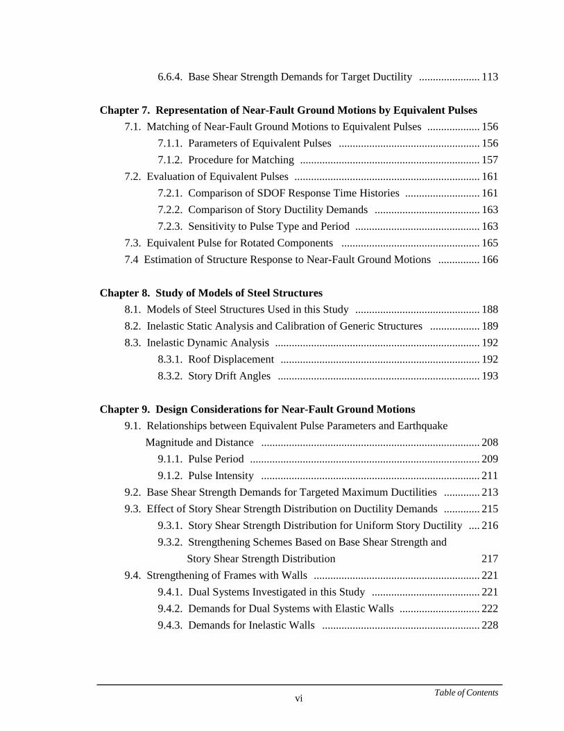
Table of Contents vi
6.6.4. Base Shear Strength Demands for Target Ductility ...................... 113 Chapter 7. Representation of Near-Fault Ground Motions by Equivalent Pulses 7.1. Matching of Near-Fault Ground Motions to Equivalent Pulses ................... 156 7.1.1. Parameters of Equivalent Pulses ................................................... 156 7.1.2. Procedure for Matching ................................................................. 157 7.2. Evaluation of Equivalent Pulses ................................................................... 161 7.2.1. Comparison of SDOF Response Time Histories ........................... 161 7.2.2. Comparison of Story Ductility Demands ...................................... 163 7.2.3. Sensitivity to Pulse Type and Period ............................................. 163 7.3. Equivalent Pulse for Rotated Components .................................................. 165 7.4 Estimation of Structure Response to Near-Fault Ground Motions ............... 166 Chapter 8. Study of Models of Steel Structures 8.1. Models of Steel Structures Used in this Study ............................................. 188 8.2. Inelastic Static Analysis and Calibration of Generic Structures .................. 189 8.3. Inelastic Dynamic Analysis .......................................................................... 192 8.3.1. Roof Displacement ........................................................................ 192 8.3.2. Story Drift Angles ......................................................................... 193 Chapter 9. Design Considerations for Near-Fault Ground Motions 9.1. Relationships between Equivalent Pulse Parameters and Earthquake Magnitude and Distance ............................................................................... 208 9.1.1. Pulse Period ................................................................................... 209 9.1.2. Pulse Intensity ............................................................................... 211 9.2. Base Shear Strength Demands for Targeted Maximum Ductilities ............. 213 9.3. Effect of Story Shear Strength Distribution on Ductility Demands ............. 215 9.3.1. Story Shear Strength Distribution for Uniform Story Ductility .... 216 9.3.2. Strengthening Schemes Based on Base Shear Strength and Story Shear Strength Distribution 217 9.4. Strengthening of Frames with Walls ............................................................ 221 9.4.1. Dual Systems Investigated in this Study ....................................... 221 9.4.2. Demands for Dual Systems with Elastic Walls ............................. 222 9.4.3. Demands for Inelastic Walls ......................................................... 228
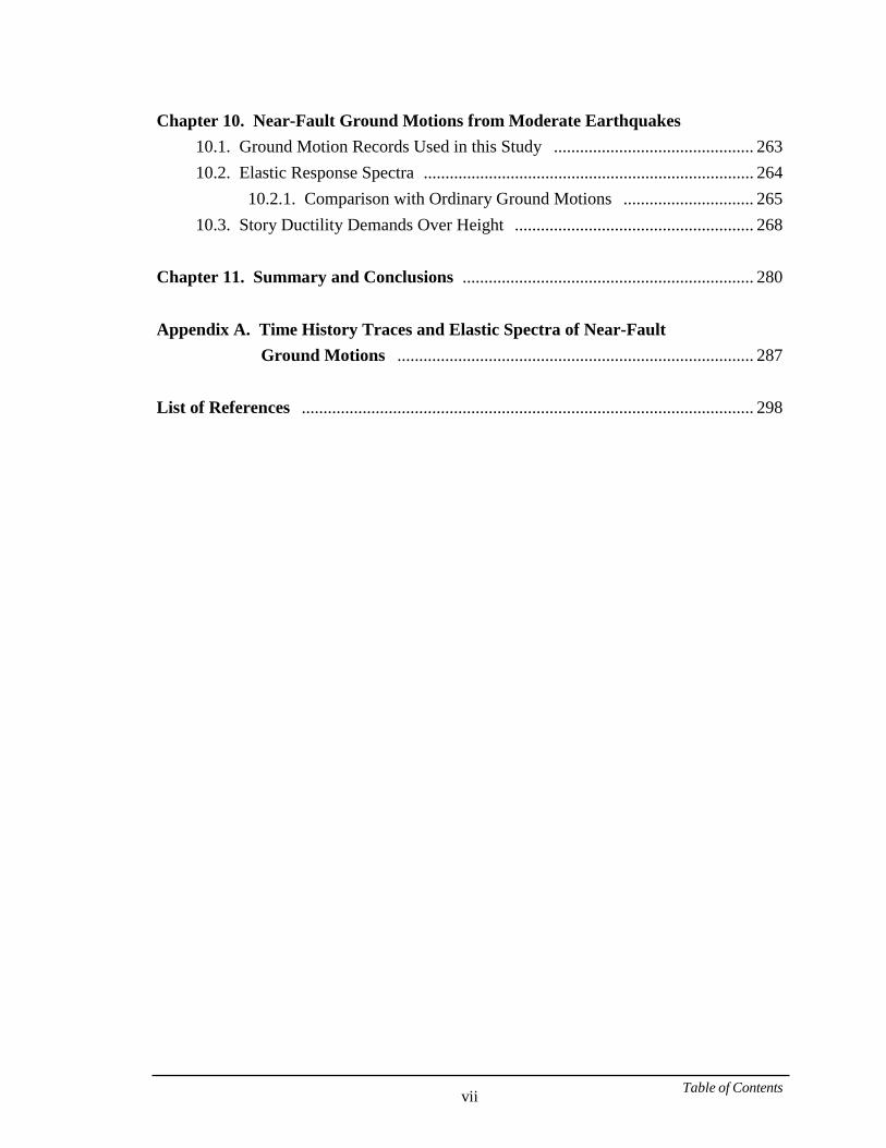
Table of Contents vii
Chapter 10. Near-Fault Ground Motions from Moderate Earthquakes 10.1. Ground Motion Records Used in this Study .............................................. 263 10.2. Elastic Response Spectra ............................................................................ 264 10.2.1. Comparison with Ordinary Ground Motions .............................. 265 10.3. Story Ductility Demands Over Height ....................................................... 268 Chapter 11. Summary and Conclusions ................................................................... 280 Appendix A. Time History Traces and Elastic Spectra of Near-Fault Ground Motions .................................................................................. 287 List of References ........................................................................................................ 298
Chapter 1 Introduction 1
CHAPTER 1
INTRODUCTION
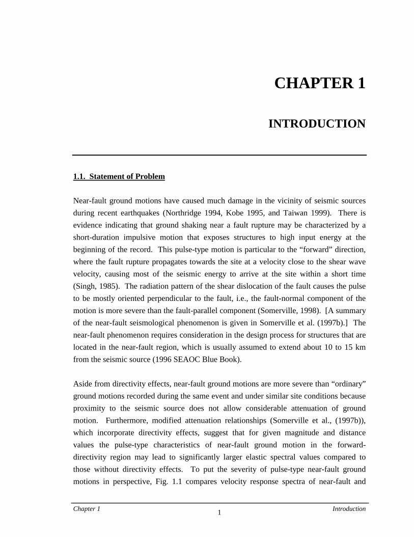
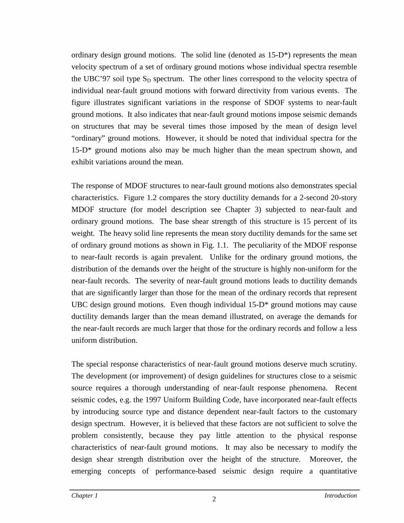
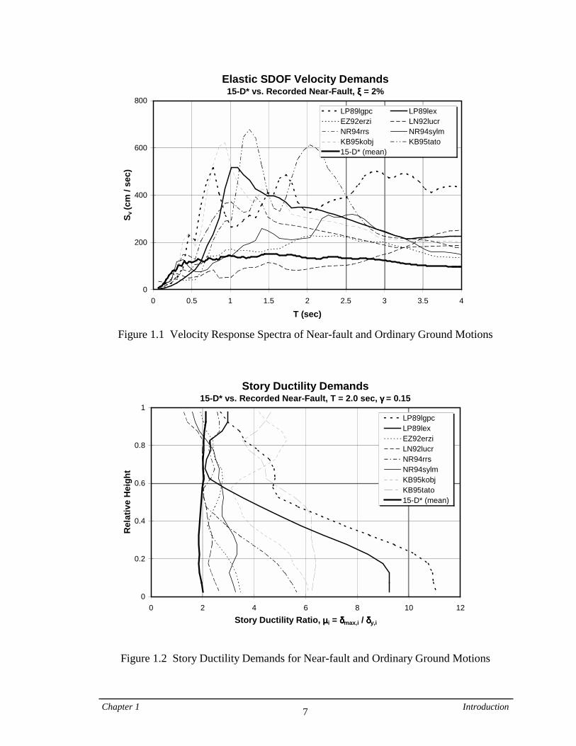
1.1. Statement of Problem Near-fault ground motions have caused much damage in the vicinity of seismic sources during recent earthquakes (Northridge 1994, Kobe 1995, and Taiwan 1999). There is evidence indicating that ground shaking near a fault rupture may be characterized by a short-duration impulsive motion that exposes structures to high input energy at the beginning of the record. This pulse-type motion is particular to the “forward” direction, where the fault rupture propagates towards the site at a velocity close to the shear wave velocity, causing most of the seismic energy to arrive at the site within a short time (Singh, 1985). The radiation pattern of the shear dislocation of the fault causes the pulse to be mostly oriented perpendicular to the fault, i.e., the fault-normal component of the motion is more severe than the fault-parallel component (Somerville, 1998). [A summary of the near-fault seismological phenomenon is given in Somerville et al. (1997b).] The near-fault phenomenon requires consideration in the design process for structures that are located in the near-fault region, which is usually assumed to extend about 10 to 15 km from the seismic source (1996 SEAOC Blue Book). Aside from directivity effects, near-fault ground motions are more severe than “ordinary” ground motions recorded during the same event and under similar site conditions because proximity to the seismic source does not allow considerable attenuation of ground motion. Furthermore, modified attenuation relationships (Somerville et al., (1997b)), which incorporate directivity effects, suggest that for given magnitude and distance values the pulse-type characteristics of near-fault ground motion in the forward-directivity region may lead to significantly larger elastic spectral values compared to those without directivity effects. To put the severity of pulse-type near-fault ground motions in perspective, Fig. 1.1 compares velocity response spectra of near-fault and
Chapter 1 Introduction 2
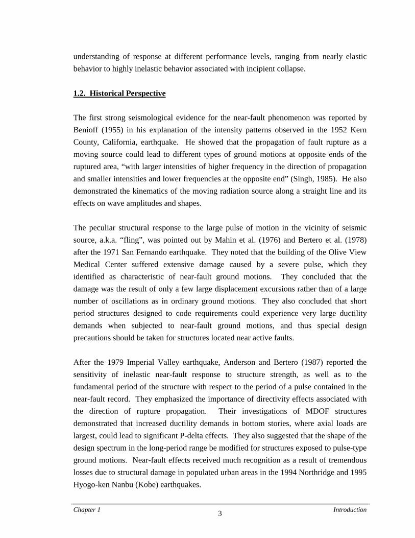
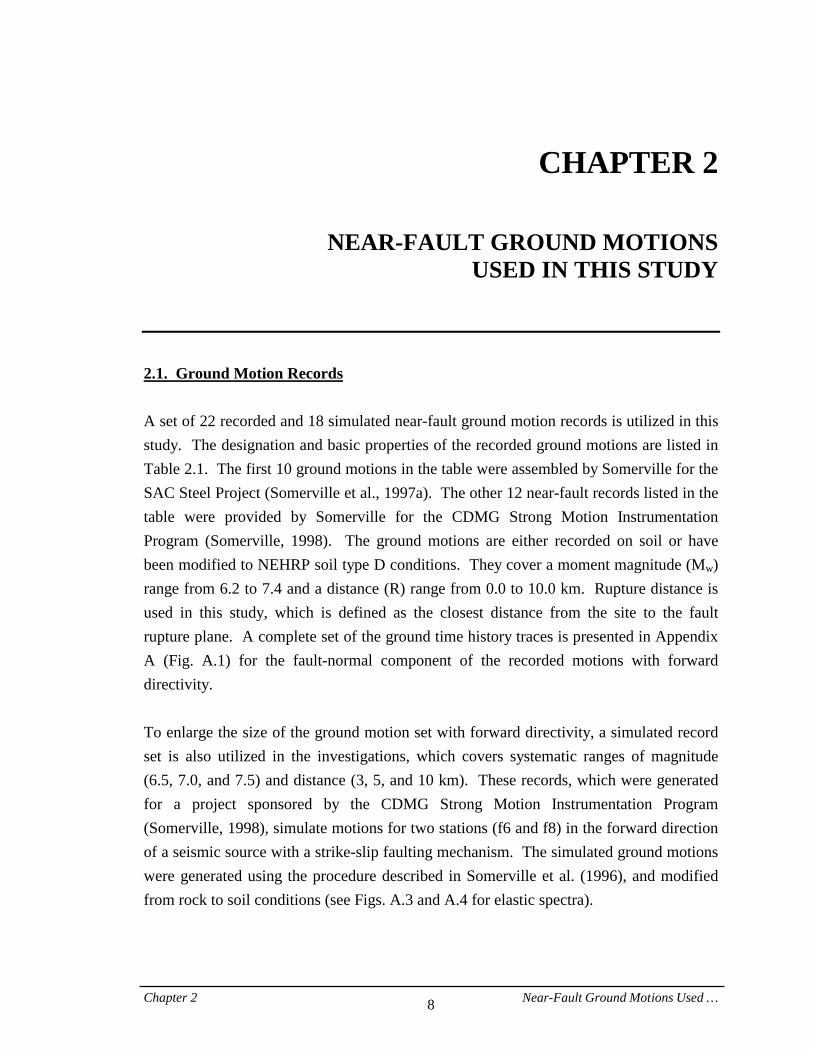
ordinary design ground motions. The solid line (denoted as 15-D*) represents the mean velocity spectrum of a set of ordinary ground motions whose individual spectra resemble the UBC’97 soil type SD spectrum. The other lines correspond to the velocity spectra of individual near-fault ground motions with forward directivity from various events. The figure illustrates significant variations in the response of SDOF systems to near-fault ground motions. It also indicates that near-fault ground motions impose seismic demands on structures that may be several times those imposed by the mean of design level “ordinary” ground motions. However, it should be noted that individual spectra for the 15-D* ground motions also may be much higher than the mean spectrum shown, and exhibit variations around the mean. The response of MDOF structures to near-fault ground motions also demonstrates special characteristics. Figure 1.2 compares the story ductility demands for a 2-second 20-story MDOF structure (for model description see Chapter 3) subjected to near-fault and ordinary ground motions. The base shear strength of this structure is 15 percent of its weight. The heavy solid line represents the mean story ductility demands for the same set of ordinary ground motions as shown in Fig. 1.1. The peculiarity of the MDOF response to near-fault records is again prevalent. Unlike for the ordinary ground motions, the distribution of the demands over the height of the structure is highly non-uniform for the near-fault records. The severity of near-fault ground motions leads to ductility demands that are significantly larger than those for the mean of the ordinary records that represent UBC design ground motions. Even though individual 15-D* ground motions may cause ductility demands larger than the mean demand illustrated, on average the demands for the near-fault records are much larger that those for the ordinary records and follow a less uniform distribution. The special response characteristics of near-fault ground motions deserve much scrutiny. The development (or improvement) of design guidelines for structures close to a seismic source requires a thorough understanding of near-fault response phenomena. Recent seismic codes, e.g. the 1997 Uniform Building Code, have incorporated near-fault effects by introducing source type and distance dependent near-fault factors to the customary design spectrum. However, it is believed that these factors are not sufficient to solve the problem consistently, because they pay little attention to the physical response characteristics of near-fault ground motions. It may also be necessary to modify the design shear strength distribution over the height of the structure. Moreover, the emerging concepts of performance-based seismic design require a quantitative
Chapter 1 Introduction 3
understanding of response at different performance levels, ranging from nearly elastic behavior to highly inelastic behavior associated with incipient collapse. 1.2. Historical Perspective The first strong seismological evidence for the near-fault phenomenon was reported by Benioff (1955) in his explanation of the intensity patterns observed in the 1952 Kern County, California, earthquake. He showed that the propagation of fault rupture as a moving source could lead to different types of ground motions at opposite ends of the ruptured area, “with larger intensities of higher frequency in the direction of propagation and smaller intensities and lower frequencies at the opposite end” (Singh, 1985). He also demonstrated the kinematics of the moving radiation source along a straight line and its effects on wave amplitudes and shapes. The peculiar structural response to the large pulse of motion in the vicinity of seismic source, a.k.a. “fling”, was pointed out by Mahin et al. (1976) and Bertero et al. (1978) after the 1971 San Fernando earthquake. They noted that the building of the Olive View Medical Center suffered extensive damage caused by a severe pulse, which they identified as characteristic of near-fault ground motions. They concluded that the damage was the result of only a few large displacement excursions rather than of a large number of oscillations as in ordinary ground motions. They also concluded that short period structures designed to code requirements could experience very large ductility demands when subjected to near-fault ground motions, and thus special design precautions should be taken for structures located near active faults. After the 1979 Imperial Valley earthquake, Anderson and Bertero (1987) reported the sensitivity of inelastic near-fault response to structure strength, as well as to the fundamental period of the structure with respect to the period of a pulse contained in the near-fault record. They emphasized the importance of directivity effects associated with the direction of rupture propagation. Their investigations of MDOF structures demonstrated that increased ductility demands in bottom stories, where axial loads are largest, could lead to significant P-delta effects. They also suggested that the shape of the design spectrum in the long-period range be modified for structures exposed to pulse-type ground motions. Near-fault effects received much recognition as a result of tremendous losses due to structural damage in populated urban areas in the 1994 Northridge and 1995 Hyogo-ken Nanbu (Kobe) earthquakes.

Chapter 1 Introduction 4
Hall et al. (1995) employed wave propagation theory to study the response of a continuous shear building to pulse-type ground motions. They, too, warned about the damaging effects of near-fault ground motions and the inadequacy of current code provisions to address the problem effectively. Iwan (1997) utilized a similar elastic shear building to obtain the “drift spectrum” (maximum story drift plotted vs. structure period) as a measure of seismic demand for MDOF structures subjected to near-fault ground motions with pulse-type characteristics. He showed that even for elastic structures near-fault effects cannot be accounted for simply by multiplying the code base shear coefficient by a near-fault factor that is constant beyond a relatively short period (as in UBC’97). Several studies have been aimed at mitigating the near-fault problem by improving the performance of structures that are exposed to near-fault ground motions. Hall et al. (1995), and Makris and Chang (2000), among others, studied the efficiency of base isolation with various dissipative mechanisms to protect structures from pulse-type and near-fault ground motions. Although there are some promising results, large displacement demands imposed by severe pulses of near-fault ground motions pose many difficulties. Anderson et al. (1999) evaluated the performance of several tall R/C and steel frames strengthened by single or coupled shear walls (for R/C frames) and lateral bracing systems (for steel frames). They concluded that when long period structures are subjected to severe pulse-type ground motions, conventional retrofit strategies, such as increasing the stiffness and/or strength of the system by adding shear walls, are not efficient. The reason is that increasing the stiffness shortens the period of the system, moving it into a range of higher spectral accelerations. They, however, argued for the use of energy dissipation devices, particularly viscous dampers, as a more effective technique to provide protection against near-fault effects. 1.3. Objectives and Scope This study attempts a systematic evaluation of the elastic and inelastic response of SDOF systems and MDOF frame structures subjected to near-fault ground motions. The global objective is to acquire quantitative knowledge on near-fault ground motion effects. The results of this study are intended to identify salient response characteristics, to describe near-fault ground motions by simple equivalent pulses, and to utilize the pulse response characteristics to define behavior attributes of structures when subjected to near-fault ground motions. The ultimate goal is to develop design guidelines or strengthening
Chapter 1 Introduction 5
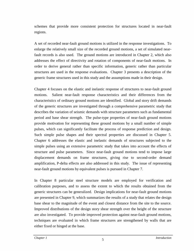
schemes that provide more consistent protection for structures located in near-fault regions. A set of recorded near-fault ground motions is utilized in the response investigations. To enlarge the relatively small size of the recorded ground motions, a set of simulated near-fault records is also used. The ground motions are introduced in Chapter 2, which also addresses the effect of directivity and rotation of components of near-fault motions. In order to derive general rather than specific information, generic rather than particular structures are used in the response evaluations. Chapter 3 presents a description of the generic frame structures used in this study and the assumptions made in their design. Chapter 4 focuses on the elastic and inelastic response of structures to near-fault ground motions. Salient near-fault response characteristics and their differences from the characteristics of ordinary ground motions are identified. Global and story drift demands of the generic structures are investigated through a comprehensive parametric study that describes the variation of seismic demands with structure parameters such as fundamental period and base shear strength. The pulse-type properties of near-fault ground motions provide motivation for representing these ground motions by a small number of simple pulses, which can significantly facilitate the process of response prediction and design. Such simple pulse shapes and their spectral properties are discussed in Chapter 5. Chapter 6 addresses the elastic and inelastic demands of structures subjected to the simple pulses using an extensive parametric study that takes into account the effects of structure and pulse parameters. Since near-fault ground motions tend to impose large displacement demands on frame structures, giving rise to second-order demand amplification, P-delta effects are also addressed in this study. The issue of representing near-fault ground motions by equivalent pulses is pursued in Chapter 7. In Chapter 8 particular steel structure models are employed for verification and calibration purposes, and to assess the extent to which the results obtained from the generic structures can be generalized. Design implications for near-fault ground motions are presented in Chapter 9, which summarizes the results of a study that relates the design base shear to the magnitude of the event and closest distance from the site to the source. Improved distributions of the design story shear strength over the height of the structure are also investigated. To provide improved protection against near-fault ground motions, techniques are evaluated in which frame structures are strengthened by walls that are either fixed or hinged at the base.
Chapter 1 Introduction 6
Chapter 10 is concerned with the study of near-fault effects in moderate earthquakes. Even though collapse safety is not a matter of concern for these earthquakes, damage control is an issue. The SDOF and MDOF response of structures to a set of ground motions recorded during events with magnitude 6.1 and smaller is investigated. The spectral properties of the ground motions are compared with those of ordinary records that form the basis for current code guidelines. Many fundamental characteristics of near-fault ground motions and their effects on frame structures have been identified and quantified in this study. But it is recognized that the near-fault problem is very complex, and that more work is needed before a comprehensive understanding of all important aspects of the problem will be accomplished. This work attempts to address the most important issues concerning near-fault ground motions and their response attributes in order to form a foundation on which to base future research and development of design guidelines.
Chapter 1 Introduction 7
Elastic SDOF Velocity Demands 15-D* vs. Recorded Near-Fault, ξξξξ===== 2%
0
200
400
600
800
0 0.5 1 1.5 2 2.5 3 3.5 4
T (sec)
S v (c
m /
sec)
LP89lgpc LP89lexEZ92erzi LN92lucrNR94rrs NR94sylmKB95kobj KB95tato15-D* (mean)
Figure 1.1 Velocity Response Spectra of Near-fault and Ordinary Ground Motions
Story Ductility Demands15-D* vs. Recorded Near-Fault, T = 2.0 sec, γγγγ = 0.15
0
0.2
0.4
0.6
0.8
1
0 2 4 6 8 10 12Story Ductility Ratio, µµµµi = δδδδmax,i / δδδδy,i
Rel
ativ
e H
eigh
t
LP89lgpcLP89lexEZ92erziLN92lucrNR94rrsNR94sylmKB95kobjKB95tato15-D* (mean)
Figure 1.2 Story Ductility Demands for Near-fault and Ordinary Ground Motions
Chapter 2 Near-Fault Ground Motions Used … 8
CHAPTER 2
NEAR-FAULT GROUND MOTIONS USED IN THIS STUDY
2.1. Ground Motion Records A set of 22 recorded and 18 simulated near-fault ground motion records is utilized in this study. The designation and basic properties of the recorded ground motions are listed in Table 2.1. The first 10 ground motions in the table were assembled by Somerville for the SAC Steel Project (Somerville et al., 1997a). The other 12 near-fault records listed in the table were provided by Somerville for the CDMG Strong Motion Instrumentation Program (Somerville, 1998). The ground motions are either recorded on soil or have been modified to NEHRP soil type D conditions. They cover a moment magnitude (Mw) range from 6.2 to 7.4 and a distance (R) range from 0.0 to 10.0 km. Rupture distance is used in this study, which is defined as the closest distance from the site to the fault rupture plane. A complete set of the ground time history traces is presented in Appendix A (Fig. A.1) for the fault-normal component of the recorded motions with forward directivity. To enlarge the size of the ground motion set with forward directivity, a simulated record set is also utilized in the investigations, which covers systematic ranges of magnitude (6.5, 7.0, and 7.5) and distance (3, 5, and 10 km). These records, which were generated for a project sponsored by the CDMG Strong Motion Instrumentation Program (Somerville, 1998), simulate motions for two stations (f6 and f8) in the forward direction of a seismic source with a strike-slip faulting mechanism. The simulated ground motions were generated using the procedure described in Somerville et al. (1996), and modified from rock to soil conditions (see Figs. A.3 and A.4 for elastic spectra).
Chapter 2 Near-Fault Ground Motions Used … 9
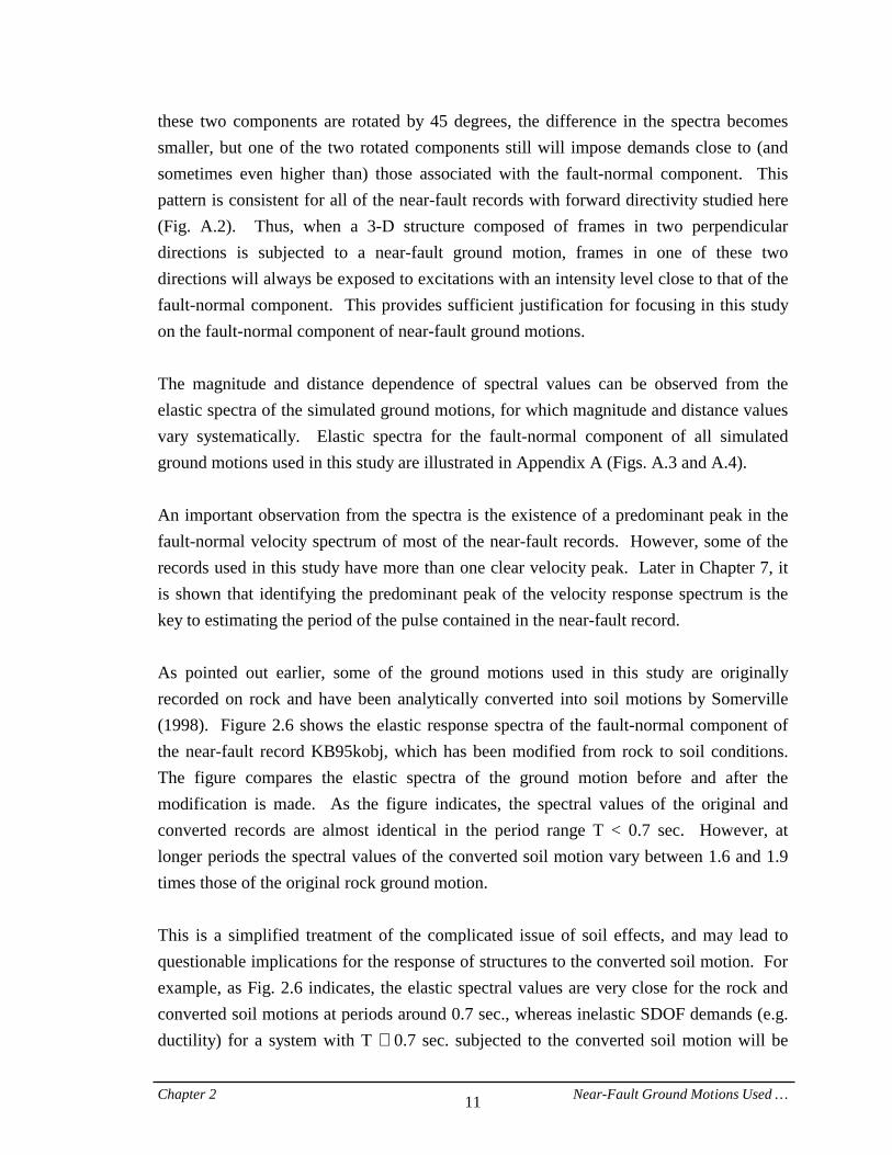
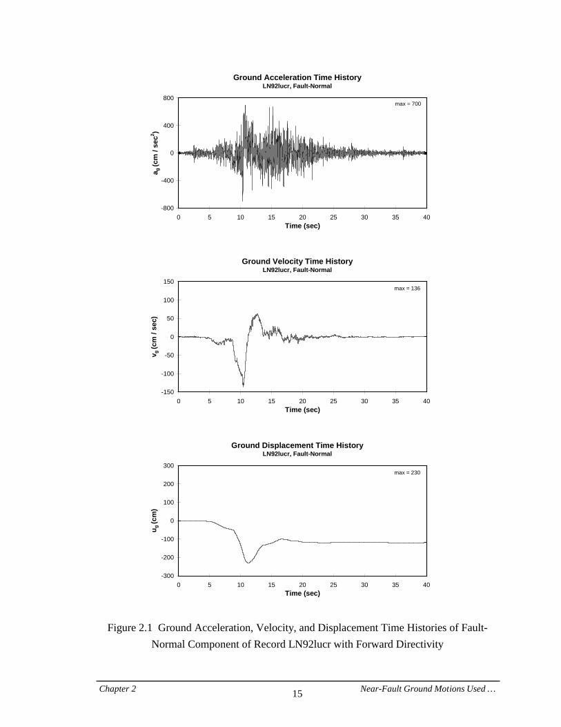
In all near-fault time histories there should be static displacements due to the static dislocation field of the earthquake. However, most recording systems do not adequately record the permanent displacements, which are filtered out of the recordings in the course of processing. Somerville has not attempted to retain the static displacement field in any of the time histories, with the exception of the Lucerne recording of the 1992 Landers earthquake (LN92lucr). This time history has been modified by Graves (1996) compared to the version of Iwan and Chen (1994) to include geodetically defined static displacements. MacRae et al. (1998) have shown that the effect of baseline correction on SDOF response to near-fault ground motions is small. 2.1.1. Directivity Effects The record set includes recordings with both forward and backward rupture directivity. If the rupture propagates towards the site, the recording at the site will show forward-directivity effects. Since the propagation occurs at a velocity that is close to the shear wave velocity, most of the seismic energy from the rupture arrives at the site in a large pulse of motion at the beginning of the record (Somerville et al., 1997b). This large pulse is mostly oriented in the fault-normal direction on account of the radiation pattern of shear dislocation on the fault. Figure 2.1 illustrates ground time history traces for the fault-normal component of a near-fault ground motion (LN92lucr) that was recorded in the forward-directivity region during the 1992 Landers earthquake (Wald and Heaton, 1994). The large pulse of motion is clearly observed in the velocity and displacement time histories. If the rupture propagates away from the site, the recording at the site will show backward-directivity effects. Records with backward directivity exhibit long-duration motions that have low amplitudes at long periods (Somerville et al., 1997b). Figure 2.2 presents the time histories for a ground motion (LN92josh) that was recorded in the backward-directivity region of the Landers earthquake. As can be seen, this record does not show the pulse-type characteristics of the type observed from records with forward directivity. Instead, the seismic energy arriving at the site is scattered throughout a long-duration ground motion. It is also observed that the maximum ground acceleration, velocity, and displacement of this backward-directivity record are significantly smaller than their corresponding values of the forward-directivity record LN92lucr, even though LN92josh is recorded at a station that is closer to the epicenter of the Landers earthquake.
Chapter 2 Near-Fault Ground Motions Used … 10
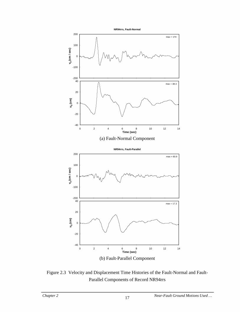
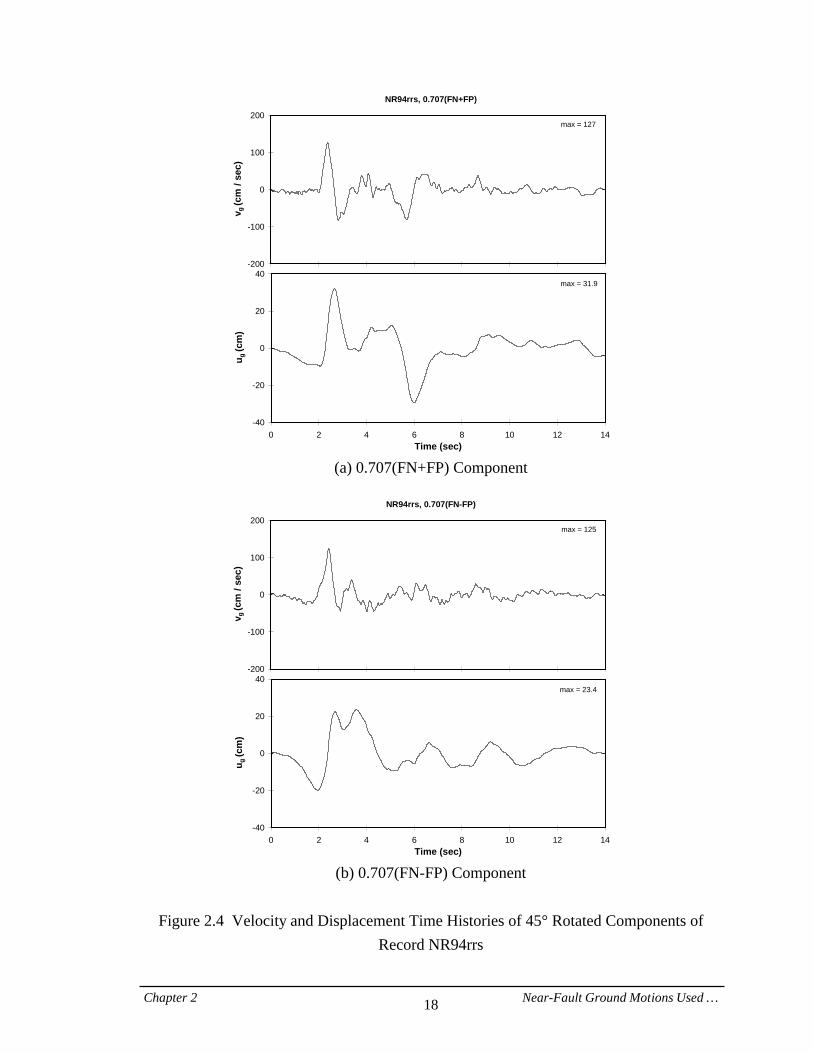
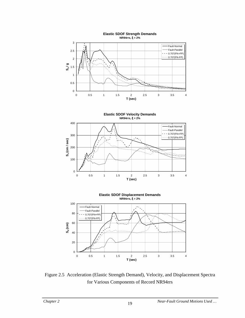
This study focuses only on the response characteristics of near-fault ground motions with forward directivity. 2.1.2. Ground Motion Components Figure 2.3 illustrates ground velocity and displacement traces for the fault-normal and fault-parallel components of the near-fault record NR94rrs. This ground motion, which was recorded in the forward-directivity region of the 1994 Northridge earthquake, shows a large pulse of motion in the fault-normal trace within the time range from 2 to 3 sec. As pointed out earlier, the fault-normal component of the motion is much more severe than the fault-parallel component due to the radiation pattern of shear dislocation. Therefore, the orientation of the structure with respect to the fault direction may determine the severity of the ground motion that the structure will experience in the near-fault region of a fault rupture. In order to obtain a better understanding of the orientation effect, Fig. 2.4 shows ground velocity and displacement time histories for two rotated components of the ground motion under consideration. These components, which are rotated by 45 degrees with respect to the fault direction, are obtained by combining the fault-normal and fault-parallel time histories. It can be seen that the two rotated components also exhibit pulse-type characteristics. The time history trace of one of the rotated components is very similar to that of the fault-normal component (Fig. 2.4(a)). Thus, it appears that pulse-type characteristics are not limited to the fault-normal direction. The study of the time history traces also suggests that the rotated components are relatively severe. The severity of the rotated components is further addressed using spectral values. 2.2. Elastic Spectra of Near-Fault Ground Motions Figure 2.5 illustrates acceleration (elastic strength demand), velocity, and displacement spectra of the near-fault ground motion NR94rrs, whose ground time histories were illustrated earlier. Each graph includes the spectra for the fault-normal, fault-parallel, and the two 45° rotated components of this ground motion. All spectra are computed for 2% damping. The figure clearly shows the large differences between the fault-normal and fault-parallel components. These results as well as the elastic spectra of other near-fault ground motions with forward directivity (see Appendix A, Fig. A.2) emphasize that the fault-normal component is much more severe than the fault-parallel component. When
Chapter 2 Near-Fault Ground Motions Used … 11
these two components are rotated by 45 degrees, the difference in the spectra becomes smaller, but one of the two rotated components still will impose demands close to (and sometimes even higher than) those associated with the fault-normal component. This pattern is consistent for all of the near-fault records with forward directivity studied here (Fig. A.2). Thus, when a 3-D structure composed of frames in two perpendicular directions is subjected to a near-fault ground motion, frames in one of these two directions will always be exposed to excitations with an intensity level close to that of the fault-normal component. This provides sufficient justification for focusing in this study on the fault-normal component of near-fault ground motions. The magnitude and distance dependence of spectral values can be observed from the elastic spectra of the simulated ground motions, for which magnitude and distance values vary systematically. Elastic spectra for the fault-normal component of all simulated ground motions used in this study are illustrated in Appendix A (Figs. A.3 and A.4). An important observation from the spectra is the existence of a predominant peak in the fault-normal velocity spectrum of most of the near-fault records. However, some of the records used in this study have more than one clear velocity peak. Later in Chapter 7, it is shown that identifying the predominant peak of the velocity response spectrum is the key to estimating the period of the pulse contained in the near-fault record. As pointed out earlier, some of the ground motions used in this study are originally recorded on rock and have been analytically converted into soil motions by Somerville (1998). Figure 2.6 shows the elastic response spectra of the fault-normal component of the near-fault record KB95kobj, which has been modified from rock to soil conditions. The figure compares the elastic spectra of the ground motion before and after the modification is made. As the figure indicates, the spectral values of the original and converted records are almost identical in the period range T < 0.7 sec. However, at longer periods the spectral values of the converted soil motion vary between 1.6 and 1.9 times those of the original rock ground motion. This is a simplified treatment of the complicated issue of soil effects, and may lead to questionable implications for the response of structures to the converted soil motion. For example, as Fig. 2.6 indicates, the elastic spectral values are very close for the rock and converted soil motions at periods around 0.7 sec., whereas inelastic SDOF demands (e.g. ductility) for a system with T ≅ 0.7 sec. subjected to the converted soil motion will be
Chapter 2 Near-Fault Ground Motions Used … 12
much larger than the corresponding demands for the same system subjected to the original rock motion. The reason is that the effective period of the inelastic system elongates and moves into the period range T > 0.7 sec., in which the spectral values for the converted record are much larger than those for the original record. The large difference in inelastic demands is a direct consequence of the scheme employed to account for soil effects. Moreover, the large ground velocities in near-fault ground motions may cause nonlinear soil response, which is not considered in this simplified soil modification method. 2.2.1. Comparison with Ordinary Ground Motions Since near-fault ground motions are recorded close to the seismic source, the ground shaking has very little time to attenuate. Thus, these ground motions are more severe than the ground motions recorded far from the rupture in the same event, even without accounting for directivity effects. Based on an empirical analysis of near-fault data, Somerville et al. (1997b) developed modifications to empirical attenuation models to account for the effect of rupture directivity on strong motion amplitudes in the near-fault region. In their directivity model, the amplitude modification factor depends on two geometrical parameters: 1) the angle between the rupture propagation direction and the direction of waves traveling from the fault to the site, and 2) the fraction of the rupture plane that lies between the hypocenter and the site. They conclude that forward directivity effects cause larger spectral response at periods longer than 0.6 sec. For example, for strike-slip faulting, maximum directivity conditions amplify the average spectral value at T = 2.0 sec. by a factor of 1.8, which can be attributed to the pulse-type nature of near-fault ground motions with forward directivity. To put the severity of near-fault ground motions in perspective, a reference set of 15 “ordinary” records is utilized for comparison purposes. These records, which were used in past studies (Seneviratna and Krawinkler, 1997), are scaled in a way such that the spectrum of each individual record matches the UBC’97 soil type SD spectrum with a minimum error, using discrete periods in the range from 0.6 to 4.0 seconds (constant velocity range). The mean acceleration response spectrum of the 15 scaled records, referred to as 15-D* (mean), is shown in Fig. 2.7 together with the UBC soil type SD spectrum (Z = 0.4) without the near-fault factor. Thus, on average, these 15-D* time histories reasonably represent the UBC design spectrum, which corresponds to a 10/50 (10% in 50 years) seismic hazard level.
Chapter 2 Near-Fault Ground Motions Used … 13
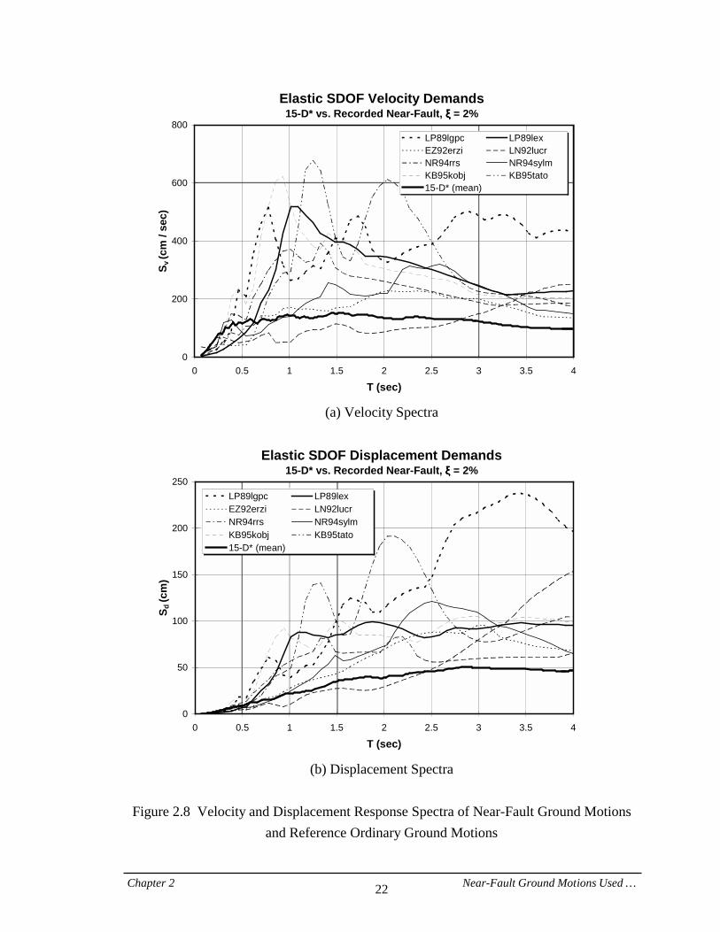
Figure 2.8 illustrates the mean velocity and displacement spectra of the 15-D* records superimposed on the velocity and displacement spectra of several of the recorded near-fault ground motions with forward directivity. This figure is presented for two reasons: first, to illustrate the great variations in the response spectra that have to be expected from near-fault ground motions, and second, to put the severity of near-fault ground motions in perspective with present design ground motions. Maximum values of spectral velocities and displacements of the near-fault records are several times those of the mean of the design ground motions. This indicates that near-fault records can impose very large demands that need to be considered in the design process. The response of MDOF structures to the near-fault ground motions represented by these spectra is discussed in Chapter 4.

Chapter 2 Near-Fault Ground Motions Used … 14
Table 2.1 Designation and Basic Properties of Recorded Near-Fault Ground Motions Used in this Study
Designation Earthquake Station Directivity Mw R (km)TB78tab Tabas, 1978 Tabas backward 7.4 1.2LP89lgpc Loma Prieta, 1989 Los Gatos forward 7.0 3.5LP89lex Loma Prieta, 1989 Lexington forward 7.0 6.3CM92petr Mendocino, 1992 Petrolia backward 7.1 8.5EZ92erzi Erzincan, 1992 Erzincan forward 6.7 2.0LN92lucr Landers, 1992 Lucerne forward 7.3 1.1NR94rrs Nothridge, 1994 Rinaldi forward 6.7 7.5NR94sylm Nothridge, 1994 Olive View forward 6.7 6.4KB95kobj Kobe, 1995 JMA forward 6.9 0.6KB95tato Kobe, 1995 Takatori forward 6.9 1.5IV79ar06 Imperial Valley, 1979 Array 6 forward 6.5 1.2IV79bond Imperial Valley, 1979 Bond's Corn backward 6.5 2.4IV79melo Imperial Valley, 1979 Meloland forward 6.5 0.0KB95kpi1 Kobe, 1995 Port Island forward 6.9 3.7LN92josh Landers, 1992 Joshua Tree backward 7.3 7.4LP89corr Loma Prieta, 1989 Corralitos backward 7.0 3.4MH84andd Morgan Hill, 1984 Anderson D forward 6.2 4.5MH84cyld Morgan Hill, 1984 Coyote L D forward 6.2 0.1MH84hall Morgan Hill, 1984 Halls Valley backward 6.2 2.4NR94newh Nothridge, 1994 Newhall forward 6.7 7.1NR94nord Nothridge, 1994 Arleta backward 6.7 9.2NR94spva Nothridge, 1994 Sepulveda forward 6.7 8.9
Chapter 2 Near-Fault Ground Motions Used … 15
Ground Acceleration Time HistoryLN92lucr, Fault-Normal
-800
-400
0
400
800
0 5 10 15 20 25 30 35 40Time (sec)
a g (c
m /
sec2 )
max = 700
Ground Velocity Time HistoryLN92lucr, Fault-Normal
-150
-100
-50
0
50
100
150
0 5 10 15 20 25 30 35 40Time (sec)
v g (c
m /
sec)
max = 136
Ground Displacement Time HistoryLN92lucr, Fault-Normal
-300
-200
-100
0
100
200
300
0 5 10 15 20 25 30 35 40Time (sec)
u g (c
m)
max = 230
Figure 2.1 Ground Acceleration, Velocity, and Displacement Time Histories of Fault-Normal Component of Record LN92lucr with Forward Directivity

Chapter 2 Near-Fault Ground Motions Used … 16
Ground Acceleration Time HistoryLN92josh, Fault-Normal
-300
-200
-100
0
100
200
300
0 5 10 15 20 25 30 35 40Time (sec)
a g (c
m /
sec2 )
max = 272
Ground Velocity Time HistoryLN92josh, Fault-Normal
-50
-25
0
25
50
0 5 10 15 20 25 30 35 40Time (sec)
v g (c
m /
sec)
max = 42.2
Ground Displacement Time HistoryLN92josh, Fault-Normal
-20
-10
0
10
20
0 5 10 15 20 25 30 35 40Time (sec)
u g (c
m)
max = 14.9
Figure 2.2 Ground Acceleration, Velocity, and Displacement Time Histories of Fault-Normal Component of Record LN92josh with Backward Directivity
Chapter 2 Near-Fault Ground Motions Used … 17
NR94rrs, Fault-Normal
-200
-100
0
100
200
v g (c
m /
sec)
max = 174
-40
-20
0
20
40
0 2 4 6 8 10 12 14Time (sec)
u g (c
m)
max = 38.3
(a) Fault-Normal Component
NR94rrs, Fault-Parallel
-200
-100
0
100
200
v g (c
m /
sec)
max = 60.9
-40
-20
0
20
40
0 2 4 6 8 10 12 14Time (sec)
u g (c
m)
max = 17.3
(b) Fault-Parallel Component
Figure 2.3 Velocity and Displacement Time Histories of the Fault-Normal and Fault-
Parallel Components of Record NR94rrs
Chapter 2 Near-Fault Ground Motions Used … 18
NR94rrs, 0.707(FN+FP)
-200
-100
0
100
200
v g (c
m /
sec)
max = 127
-40
-20
0
20
40
0 2 4 6 8 10 12 14Time (sec)
u g (c
m)
max = 31.9
(a) 0.707(FN+FP) Component
NR94rrs, 0.707(FN-FP)
-200
-100
0
100
200
v g (c
m /
sec)
max = 125
-40
-20
0
20
40
0 2 4 6 8 10 12 14Time (sec)
u g (c
m)
max = 23.4
(b) 0.707(FN-FP) Component
Figure 2.4 Velocity and Displacement Time Histories of 45° Rotated Components of
Record NR94rrs
Chapter 2 Near-Fault Ground Motions Used … 19
Elastic SDOF Strength DemandsNR94rrs, ξξξξ = 2%
0
0.5
1
1.5
2
2.5
3
0 0.5 1 1.5 2 2.5 3 3.5 4T (sec)
S a /
g
Fault-NormalFault-Parallel0.707(FN+FP)0.707(FN-FP)
Elastic SDOF Velocity DemandsNR94rrs, ξξξξ = 2%
0
100
200
300
400
0 0.5 1 1.5 2 2.5 3 3.5 4T (sec)
S v (c
m /
sec)
Fault-NormalFault-Parallel0.707(FN+FP)0.707(FN-FP)
Elastic SDOF Displacement DemandsNR94rrs, ξξξξ = 2%
0
20
40
60
80
100
0 0.5 1 1.5 2 2.5 3 3.5 4T (sec)
S d (c
m)
Fault-NormalFault-Parallel0.707(FN+FP)0.707(FN-FP)
Figure 2.5 Acceleration (Elastic Strength Demand), Velocity, and Displacement Spectra for Various Components of Record NR94rrs

Chapter 2 Near-Fault Ground Motions Used … 20
Elastic SDOF Strength DemandsKB95kobj, Fault-Normal, ξξξξ = 2%
0
1
2
3
4
5
0 0.5 1 1.5 2 2.5 3 3.5 4T (sec)
S a /
g
Rock
Soil
Elastic SDOF Velocity DemandsKB95kobj, Fault-Normal, ξξξξ = 2%
0
200
400
600
800
0 0.5 1 1.5 2 2.5 3 3.5 4T (sec)
S v (c
m /
sec)
Rock
Soil
Elastic SDOF Displacement DemandsKB95kobj, Fault-Normal, ξξξξ = 2%
0
20
40
60
80
100
120
0 0.5 1 1.5 2 2.5 3 3.5 4T (sec)
S d (c
m)
Rock
Soil
Figure 2.6 Comparison of Elastic Spectra of Original (Rock) and Converted (Soil) Motions for Fault-Normal Component of Record KB95kobj

Chapter 2 Near-Fault Ground Motions Used … 21
Elastic SDOF Strength Demand Spectra15-D* Records and UBC 97 Soil Type SD, ξξξξ = 5%
0
0.4
0.8
1.2
1.6
2
0 0.5 1 1.5 2 2.5 3 3.5 4
T (sec)
S a (g
)UBC 97
15-D* (mean)
Figure 2.7 Mean Acceleration (Elastic Strength Demand) Spectrum of Reference Set of Records (15-D*) Superimposed on UBC’97 Soil Type SD Spectrum
Chapter 2 Near-Fault Ground Motions Used … 22
Elastic SDOF Velocity Demands 15-D* vs. Recorded Near-Fault, ξξξξ===== 2%
0
200
400
600
800
0 0.5 1 1.5 2 2.5 3 3.5 4
T (sec)
S v (c
m /
sec)
LP89lgpc LP89lexEZ92erzi LN92lucrNR94rrs NR94sylmKB95kobj KB95tato15-D* (mean)
(a) Velocity Spectra
Elastic SDOF Displacement Demands
15-D* vs. Recorded Near-Fault, ξξξξ===== 2%
0
50
100
150
200
250
0 0.5 1 1.5 2 2.5 3 3.5 4
T (sec)
S d (c
m)
LP89lgpc LP89lexEZ92erzi LN92lucrNR94rrs NR94sylmKB95kobj KB95tato15-D* (mean)
(b) Displacement Spectra
Figure 2.8 Velocity and Displacement Response Spectra of Near-Fault Ground Motions
and Reference Ordinary Ground Motions
Chapter 3 MDOF and SDOF Systems Used … 23
CHAPTER 3
SDOF AND MDOF SYSTEMS USED IN THIS STUDY
3.1. SDOF Systems Fundamental studies are carried out with elastic and inelastic SDOF systems in order to capture basic response characteristics that differentiate near-fault ground motions from “ordinary” ground motions. The elastic period T of the SDOF system is varied at closely spaced intervals to provide accurate spectral information within the range of interest. For recorded ground motions the period range is between 0 and 4.0 seconds, and for pulse-type ground motions the primary range of interest for T/Tp is between 0 and 3.0, where Tp is the period of the pulse. In most of the studies, a damping ratio of ξ = 2% is used rather than the more customary value of 5%. The reason is that the focus of the study is on steel frame structures for which 5% damping is difficult to justify. Inelastic SDOF systems are typically defined by non-degrading bilinear hysteresis rules. The yield strength is denoted as Fy, and the strain-hardening ratio is represented by α. A value of α = 0.03 is used to model hardening that is representative of typical steel frame structures. 3.2. MDOF Systems 3.2.1. Properties of Generic Structure One of the main objectives of this study is to quantify the seismic demands of multistory frame structures subjected to near-fault ground motions and simple pulses. To achieve this goal, a generic 2-dimensional frame structure is used whose strength and stiffness properties are tuned to specific requirements in order to facilitate interpretation and generalization of response results. In this generic structure, the fundamental elastic
Chapter 3 MDOF and SDOF Systems Used … 24
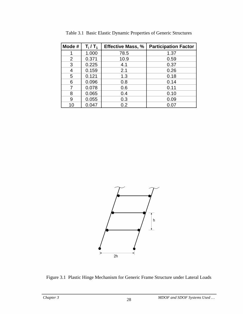
period T is a variable, but the number of stories is kept constant at 20. It was considered impractical to vary the number of stories because of the emphasis on pulse loading, which is characterized by a pulse period Tp rather than a specific numerical value of T that can be associated with a specific number of stories. However, the sensitivity of response to the number of stories will be studied in Section 6.5. In its physical configuration, the generic structure is a single-bay moment-resisting frame whose story strengths and stiffnesses are tuned to specific requirements that are discussed in the next section. Inelastic deformations are permitted only at the ends of the beam in each story and at the base of the columns. Thus, the basic plastic hinge mechanism under lateral loads involves all stories, with no individual story mechanism allowed. This mechanism, which is illustrated in Fig. 3.1, represents structures that comply with the “weak beam – strong column” provisions of current seismic codes. Structures that can form story mechanisms will be studied in Section 6.6. Response to near-fault ground motions is affected by many variables. This study is intended to shed light on near-fault response characteristics in general terms, while keeping the results useful for practical purposes. This requires that the assumptions made in the design of the generic structure be realistic enough to keep the results practical, but not too specific to compromise generality. The following assumptions are made in the design of the generic model structure: • = Floor mass is the same in every story and at the roof level. • = Story height is the same in every story. • = Bay width is twice the story height. • = Beam and column moments of inertia are the same in each story. • = Only flexural deformations are considered. • = The variation of the moment of inertia over the height is tuned such that the later
defined SRSS lateral load pattern results in a straight-line deflected shape of the structure.
• = The beam bending strength in each story is tuned such that under the SRSS lateral load pattern simultaneous yielding occurs in all stories.
• = The effect of gravity load moments on plastic hinge formation is not considered. • = A bilinear non-degrading hysteresis model with a 3% strain-hardening ratio is used at
all plastic hinge locations.
Chapter 3 MDOF and SDOF Systems Used … 25
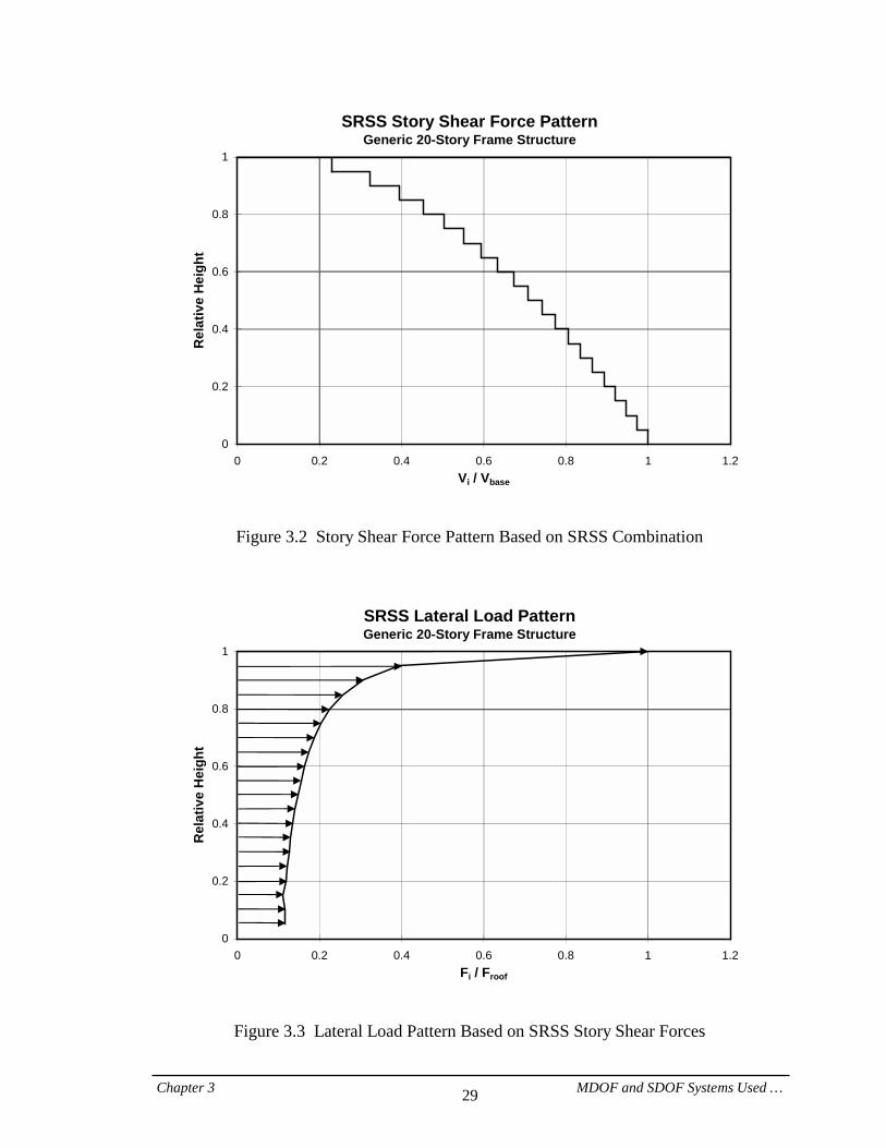
Some of the assumptions will be revisited in the later chapters. In Chapter 8 the representativeness of the generic structure will be evaluated using models of multi-story steel frames. For time history analyses, Rayleigh damping is used to obtain a damping ratio of 2% at the first mode period T and at 0.1T. All MDOF structural analyses in this study are performed using the DRAIN-2DX computer program (Prakash et al., 1993). Caution should be exercised in the interpretation of results because the assumptions made here cannot represent the properties of all real structures. For example, the story stiffness and strength of multi-story frame structures typically do not change in every story, which may cause a concentration of demands where there is a discontinuity in structure properties. 3.2.2. Design Load Pattern In order to establish story stiffness and strength properties, a design lateral load pattern and base shear strength are required. The base shear yield strength is varied according to specific objectives of the analysis and is discussed later. Given the base shear yield strength, the individual story shear yield strengths are tuned to the story shear forces obtained from the design load pattern. As a result, all stories will yield simultaneously if the lateral loads follow the design load pattern. Thus, global and story “shear force-drift” relationships obtained from a pushover analysis with the design load pattern will mimic the bilinear shape corresponding to the SDOF systems summarized in Section 3.1. In previous studies by Nassar and Krawinkler (1991), and Seneviratna and Krawinkler (1997), the UBC seismic load pattern was used for stiffness and strength design of generic models. In this study it was decided to utilize a load pattern that is based on dynamic properties rather than code assumptions. A load pattern was selected for this purpose that is based on story shear forces obtained from the SRSS modal superposition method. The SRSS analysis requires the selection of a design spectrum. It is assumed that the design spectrum follows a 1/T shape for acceleration (or constant velocity) at all modal periods that contribute significantly to the SRSS combination. This assumption, together with the requirement that the deflected shape under the design load pattern should be a straight line, results in the story shear force and design load patterns illustrated in Figs. 3.2 and 3.3. It should be noted that the spectral shape used in the
Chapter 3 MDOF and SDOF Systems Used … 26
SRSS combination may not be suitable for short structures. However, to be consistent, the same spectral shape is used regardless of the period. Short structures will be investigated in Section 6.5. Since the story shear forces obtained from the SRSS combination depend on relative story stiffnesses, an iterative procedure is required to tune the element stiffnesses so that a straight-line deflected shape is obtained under the SRSS load pattern. Basic dynamic properties of the generic structure (period ratios, effective masses, and modal participation factors for modes normalized to unity at the roof level) that fulfill the stiffness design requirements are listed in Table 3.1. 3.2.3. P-Delta Effects It is expected that dynamic P-delta effects will be of major concern for structures subjected to the large displacement pulses of near-fault ground motions, particularly if inelastic interstory drifts become large and lead to ratcheting of the seismic response (Gupta and Krawinkler, 2000). To simulate P-delta effects, identical gravity loads are assigned to each story. This implies that axial column forces due to gravity loads increase linearly from the top to the bottom of the frame. The magnitude of the story gravity load is determined so that in the first story the elastic second-order interstory drift is 10% of the first-order interstory drift under the SRSS lateral loads. This is equivalent to a “stability coefficient” of 10% in the first story, i.e., θ1 = (P.∆1)/(V.h1) = 0.1, where P is the total vertical gravity load, ∆1 is the elastic first-story drift caused by the base shear V, and h1 denotes the height of the first story. In the elastic range the consequence of incorporating P-delta effects is a 10% reduction in elastic stiffness in the first story, and a smaller reduction in higher stories. In this study the stability coefficient θ1 = 0.1 is used for the generic structure regardless of the period. In reality this value will be too large for short period structures with few stories, resulting in overestimating P-delta effects. Nevertheless, the value of θ1 is kept constant because the period of the structure is best described relative to a pulse period, which varies depending on the characteristics of the near-fault ground motion. In typical US practice, steel structures consist of perimeter moment resisting frames and interior gravity frames with simple connections. It is recognized that these gravity

Chapter 3 MDOF and SDOF Systems Used … 27
frames, which are not incorporated in this study, contribute to the lateral stiffness and strength of the system, and may significantly reduce P-delta effects (Gupta and Krawinkler, 2000). The effect of P-delta on inelastic behavior is illustrated in Fig. 3.4, which shows (a) base shear versus roof displacement, and (b) base shear versus first story displacement diagrams obtained from a pushover analysis. Results without and with consideration of P-delta effects are presented. The following observations can be made:
• = If P-delta effects are neglected (without P-delta), the global and interstory strain-hardening stiffnesses are 3.7% and 3.6% of the elastic stiffness, respectively. These values are different from the 3% strain hardening assumed at plastic hinge locations, because the columns remain elastic after the beam plastic hinges have formed, and contribute to the stiffness in the post-elastic range.
• = Incorporating P-delta effects decreases the elastic stiffness by 10%, and decreases
the strain-hardening ratio from +3.7% to -14.4% for the global response, and from +3.6% to -2.8% for the first story response. The large effect on the global response is due to the cumulative nature of the global displacement response (summation of all story drifts). The fact that the decrease of post-elastic stiffness in the first story is less than 10% of the elastic stiffness is attributed to the change in the deflected shape of the structure once a mechanism has formed.
Chapter 3 MDOF and SDOF Systems Used … 28
Table 3.1 Basic Elastic Dynamic Properties of Generic Structures
Mode # Ti / T1 Effective Mass, % Participation Factor1 1.000 78.5 1.372 0.371 10.9 0.593 0.225 4.1 0.374 0.159 2.1 0.265 0.121 1.3 0.186 0.096 0.8 0.147 0.078 0.6 0.118 0.065 0.4 0.109 0.055 0.3 0.09
10 0.047 0.2 0.07
h
2h
Figure 3.1 Plastic Hinge Mechanism for Generic Frame Structure under Lateral Loads
Chapter 3 MDOF and SDOF Systems Used … 29
SRSS Story Shear Force PatternGeneric 20-Story Frame Structure
0
0.2
0.4
0.6
0.8
1
0 0.2 0.4 0.6 0.8 1 1.2Vi / Vbase
Rel
ativ
e H
eigh
t
Figure 3.2 Story Shear Force Pattern Based on SRSS Combination
SRSS Lateral Load PatternGeneric 20-Story Frame Structure
0
0.2
0.4
0.6
0.8
1
0 0.2 0.4 0.6 0.8 1 1.2Fi / Froof
Rel
ativ
e H
eigh
t
Figure 3.3 Lateral Load Pattern Based on SRSS Story Shear Forces

Chapter 3 MDOF and SDOF Systems Used … 30
Roof Displacement vs. Base ShearGeneric 20-Story Structure, SRSS Load Pattern, ααααelement = 3%
0
0.2
0.4
0.6
0.8
1
1.2
0 0.5 1 1.5 2 2.5δδδδroof====////====δδδδroof,y
V bas
e / V
base
,y
without P-delta
with P-delta
α = -14.4%
α = 3.7%
(a) Roof
First Story Drift vs. Base Shear
Generic 20-Story Structure, SRSS Load Pattern, ααααelement = 3%
0
0.2
0.4
0.6
0.8
1
1.2
0 0.5 1 1.5 2 2.5δδδδ1====////====δδδδ1,y
V bas
e / V
base
,y
without P-delta
with P-deltaα = 3.6%
α = -2.8%
(b) First Story
Figure 3.4 Global and First Story Pushover Results with and without P-Delta
Chapter 4 Response of Structures to Near-Fault … 31
CHAPTER 4
RESPONSE OF STRUCTURES TO NEAR-FAULT GROUND MOTIONS
This part of the study is devoted to evaluating and quantifying the elastic and inelastic response of SDOF and MDOF structures to near-fault ground motions. Attempts are made to characterize important response characteristics of near-fault records. The near-fault ground motions introduced in Chapter 2 and the structure models introduced in Chapter 3 are utilized in the response evaluations. In most of this chapter, two near-fault records NR94rrs and KB95kobj are used for illustration, but the observed behavior patterns hold also for other near-fault ground motions with forward directivity. Structures with various base shear strength levels are investigated to identify near-fault behavior patterns at different performance levels. The reference ground motion set introduced in Section 2.2.1 is used to emphasize major differences in the inelastic response of MDOF structures subjected to near-fault and ordinary ground motions. 4.1. Elastic Response of MDOF Structures 4.1.1. Elastic Base Shear Demands Examples of elastic base shear demands for the generic structures subjected to the fault-normal component of near-fault ground motions are presented in Fig. 4.1. Each graph compares the maximum MDOF base shear forces for structures with various fundamental periods with the corresponding elastic SDOF strength demand spectrum. There is a rather close agreement between the MDOF and SDOF results. The general observation is that the MDOF base shear demand is smaller than the first mode SDOF strength demand if higher-mode effects are not significant, and is larger than the SDOF demand if higher-mode effects are significant (large peaks in spectrum at second and/or
Chapter 4 Response of Structures to Near-Fault … 32
third mode periods). The design implication is that if the elastic design spectrum incorporates the effects of near-fault ground motions, elastic MDOF base shear demands follow patterns similar to those for ordinary ground motions (see Seneviratna and Krawinkler, 1997). 4.1.2. Elastic Shear Force Distribution Over Height of Structure Figures 4.2 and 4.3 compare the SRSS story shear strength distribution, which was used in the design of the generic structure (denoted as “Design”), with the elastic story shear force distributions obtained from (a) time history analyses, and (b) SRSS modal combinations for ground motions NR94rrs and KB95kobj, using MDOF systems with various fundamental periods T. The following observations can be made from these figures:
• = The results of the time history analyses indicate that for structures with a fundamental period ≤ 1.0 sec., the story shear force distributions are smooth and relatively close to the design distribution.
• = The distributions of the story shear forces over the height for long period systems
differ significantly from the design distribution and exhibit the effect of a wave traveling up the structure. It appears that the traveling wave effect dominates the MDOF response of structures whose fundamental period is longer than a particular value that depends on the properties of the pulse contained in the near-fault ground motion. Several researchers, e.g. Hall et al. (1995) and Iwan (1997), have studied the traveling wave in structures subjected to near-fault and pulse-type ground motions by means of elastic wave propagation theory rather than time history dynamic analysis, which was used in this study. Later in Section 6.1.2 elastic demands obtained using these two methods will be compared for pulse-type ground motions.
• = The SRSS modal superposition technique can capture only partially the traveling
wave effect. For short period structures, the distribution of story shear forces obtained from the SRSS analysis is close to the corresponding distribution obtained from the time history analysis, whereas for long period structures larger differences can be seen. The reason is that in long period structures the wave
Chapter 4 Response of Structures to Near-Fault … 33
traveling up the structure gives rise to higher-mode effects, which are not taken into account accurately by the SRSS modal combination.
The significant deviation of the elastic story shear force distribution obtained from a time history analysis from that of the design distribution indicates that presently employed design story shear strength distributions will lead to early yielding of upper stories in structures with a long fundamental period. The reason is a traveling wave effect caused by the pulse-type nature of near-fault ground motions. The effect of this traveling wave on inelastic demands for MDOF structures is investigated in Section 4.2.2. 4.1.3. Elastic Roof Displacement Demands Figure 4.4 illustrates ratios of the elastic MDOF roof displacement demand to the first-mode spectral displacement, δroof,max/Sd, for structure with various periods T, subjected to the fault-normal component of typical near-fault records. Each graph includes two curves, one for MDOF systems in which P-delta effects are neglected, and the other for systems with P-delta effects. When P-delta effects are considered, the fundamental period of the structure slightly elongates because the secondary effects reduce the effective stiffness of the structure. This is manifested in Fig. 4.4 by a small shift of the periods to the right. The first mode participation factor (PF1) is 1.37, which is equivalent to δroof,max/Sd when only the first mode of the structure is taken into account. Different patterns of deviation from this reference value for different ground motions emphasize the uniqueness of the near-fault records. The following observations can be made from the figure:
• = The general pattern is that the ratio oscillates about the predicted value of PF1 for relatively short periods, and usually exceeds the predicted value by a large amount at long periods. This observation does not comply with the results of the study performed by Seneviratna and Krawinkler (1997) for ordinary ground motions. This indicates that higher-mode effects are more significant in long period MDOF systems subjected to near-fault ground motions. The reason lies in the spectral shape of near-fault ground motions. As Fig. 4.4 indicates, for a given record the δroof,max/Sd ratio is largest for a structure whose second mode period (T2 = 0.37 T [see Table 3.1]) corresponds to a large peak in the elastic acceleration spectrum. Since this large peak for the record LN92lucr is at a period longer than
Chapter 4 Response of Structures to Near-Fault … 34
4.0 seconds, the δroof,max/Sd ratio does not exceed 1.5 within the period range investigated.
• = Figure 4.4 shows that if the period elongation due to secondary effects is
accounted for in the computation of the first mode spectral displacement (Sd), the ratio of δroof,max/Sd will be close to the corresponding ratio obtained when P-delta effects are neglected.
4.2. Ductility Demands for Inelastic Structures In this part of the study ductility demands for inelastic SDOF and MDOF systems subjected to near-fault ground motions are investigated. For MDOF systems the base shear yield strength is quantified by a base shear coefficient, γ, defined as:
γ = =Vmg
VW
y y
(4.1)
where Vy is the base shear strength, g is the acceleration of gravity, and W and m are the seismically effective weight and mass of the structure, respectively. Once the base shear strength is defined, the distribution of strength over the height follows an SRSS story shear strength pattern obtained from a constant velocity spectrum, which was discussed in Section 3.2.2. The yield strength of SDOF systems is defined using the same coefficient, γ, by substituting the SDOF yield strength, Fy, for the base shear strength, Vy, in Eq. 4.1. 4.2.1. SDOF Systems Displacement Response Time History: Figure 4.5 illustrates inelastic displacement response time histories for SDOF systems with various fundamental periods subjected to near-fault ground motions LP89lex and NR94rrs. In each case the strength of the SDOF system is selected such that a ductility ratio (µ = umax/uy) of 6 is obtained. The displacement time history values are normalized by the yield displacement uy for the corresponding structure period and input ground motion. The figure clearly demonstrates that the response to the near-fault ground motions is one-sided, with no more than two large inelastic excursions followed by small
Chapter 4 Response of Structures to Near-Fault … 35
elastic cycles. These pulse-type response characteristics differentiate near-fault ground motions from ordinary ground motions. These observations invite the conjecture that the response of structures to near-fault records can be replicated using pulse shapes as the input motion. Identifying such pulse shapes is one of the main objectives of this study. Constant Ductility Strength Demand Spectra: Figure 4.6 shows examples of elastic (µ = 1) and constant ductility inelastic strength demand spectra for the fault-normal component of near-fault records NR94rrs and KB95kobj. As discussed in Section 3.1, the results are computed for a non-degrading bilinear skeleton curve with a strain-hardening ratio of 3%. The inelastic spectra are presented for target ductility ratios µ = 2, 3, 4, 6, and 8. Similar to observations made in past studies (Nassar and Krawinkler, 1991, and Rahnama and Krawinkler, 1993), the humps of the elastic spectra diminish and even disappear at large ductility ratios. At the same time, the smaller peaks and valleys of the inelastic spectra shift to lower periods, which can be rationalized by the fact that the “effective period” of the structure elongates when the ductility increases. In order to evaluate the sensitivity of the inelastic strength demands to the hysteresis model for near-fault ground motions, inelastic SDOF strength demand spectra are computed also using the modified Clough model (see Rahnama and Krawinkler, 1993, for hysteresis rules). Figure 4.7 illustrates ratios of the strength demands obtained from the modified Clough model to the corresponding demands obtained from the bilinear model for target ductility ratios µ = 2, 3, 4, 6, and 8. The figure shows the ratios for structures with various periods T subjected to records NR94rrs and KB95kobj, which represent the near-fault ground motions with forward directivity introduced in Chapter 2. The following observations can be made:
• = For the ground motion NR94rrs and a given target ductility, the ratios are very close to 1.0 except for a narrow range of period in which the strength demands become more sensitive to the hysteresis model. This period range depends on the target ductility ratio. Most of the sensitivity is observed in the moderate to short period rage (T < 2.0 sec.).
• = For the ground motion KB95kobj, there is a large fluctuation of the ratios, which
is not limited to narrow ranges of period. The larger ratios, especially for T > 1.0
Chapter 4 Response of Structures to Near-Fault … 36
sec., indicate that the strength demands for KB95kobj are more sensitive to the hysteresis model compared to NR94rrs. Later in Chapter 7 it will be shown that KB95kobj contains a pulse with more cycles than the pulse contained by NR94rrs.
The conclusion is that particularly for ground motions that contain pulses with multiple cycles, sensitivity to the hysteresis model may not be negligible. Ductility Demands for Various Strength Levels and Periods: Figures 4.8 and 4.9 present ductility demands of SDOF systems, subjected to near-fault records NR94rrs and KB95kobj, versus (a) the normalized yield strength γ, and (b) the strength reduction factor defined as R = Fy,e/Fy(µ), where Fy,e is the elastic strength demand and Fy(µ) is the inelastic strength demand corresponding to the ductility µ. In order to evaluate the effect of the structure period, the variation of the ductility demands with the yield strength or the strength reduction factor is presented for selected period values T = 0.5, 1.0, 1.5, 2.0, 2.5, 3.0 and 4.0 seconds. The following observations are made:
• = In many cases the ductility demand, µ, varies almost linearly with the strength reduction factor, R, particularly in the large ductility range.
• = For very short period structures (T = 0.5 sec.) µ is larger than R at all ductility
values larger than 1.0, which indicates that the inelastic displacement is larger than the elastic displacement (δin/δel = µ/R).
• = For a given ductility ratio, R becomes larger than µ beyond a certain period
(between 0.5 and 1.0 sec. for the two records investigated here). Later in Chapter 6 it will be shown that this period depends on the period of the pulse contained in the near-fault ground motion.
• = At very long periods, µ approaches R, which indicates that the inelastic and
elastic displacements are close, both approaching the maximum ground displacement. Figure 4.9(b) indicates that for the record KB95kobj the equal-displacement condition will occur at periods longer than 4.0 sec.
Chapter 4 Response of Structures to Near-Fault … 37
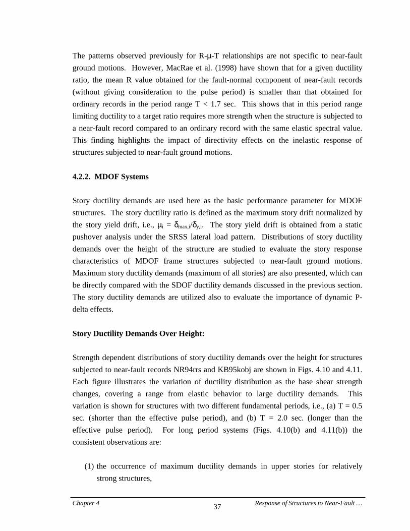
The patterns observed previously for R-µ-T relationships are not specific to near-fault ground motions. However, MacRae et al. (1998) have shown that for a given ductility ratio, the mean R value obtained for the fault-normal component of near-fault records (without giving consideration to the pulse period) is smaller than that obtained for ordinary records in the period range T < 1.7 sec. This shows that in this period range limiting ductility to a target ratio requires more strength when the structure is subjected to a near-fault record compared to an ordinary record with the same elastic spectral value. This finding highlights the impact of directivity effects on the inelastic response of structures subjected to near-fault ground motions. 4.2.2. MDOF Systems Story ductility demands are used here as the basic performance parameter for MDOF structures. The story ductility ratio is defined as the maximum story drift normalized by the story yield drift, i.e., µi = δmax,i/δy,i. The story yield drift is obtained from a static pushover analysis under the SRSS lateral load pattern. Distributions of story ductility demands over the height of the structure are studied to evaluate the story response characteristics of MDOF frame structures subjected to near-fault ground motions. Maximum story ductility demands (maximum of all stories) are also presented, which can be directly compared with the SDOF ductility demands discussed in the previous section. The story ductility demands are utilized also to evaluate the importance of dynamic P-delta effects. Story Ductility Demands Over Height: Strength dependent distributions of story ductility demands over the height for structures subjected to near-fault records NR94rrs and KB95kobj are shown in Figs. 4.10 and 4.11. Each figure illustrates the variation of ductility distribution as the base shear strength changes, covering a range from elastic behavior to large ductility demands. This variation is shown for structures with two different fundamental periods, i.e., (a) T = 0.5 sec. (shorter than the effective pulse period), and (b) T = 2.0 sec. (longer than the effective pulse period). For long period systems (Figs. 4.10(b) and 4.11(b)) the consistent observations are:
(1) the occurrence of maximum ductility demands in upper stories for relatively strong structures,
Chapter 4 Response of Structures to Near-Fault … 38
(2) the consequent stabilization (no further growth) of the story ductility demand in the upper portion, and
(3) the migration of demands toward the base as the structure becomes weaker.
However, these phenomena are not observed for short period structures (Figs. 4.10(a) and 4.11(a)). For short period structures, the maximum ductility demands occur close to the base even at high strength values, indicating that the traveling wave effect, which causes early yielding in upper stories, only occurs in structures with a long period (longer than the period of the effective pulse). The reason for the early inelastic behavior in the top portion of long period strong structures is that, as Figs. 4.2(a) and 4.3(a) indicate, the traveling wave effect in long period systems causes the elastic shear forces in upper stories to be the first to reach the story shear capacities (which follow the SRSS distribution). This leads to premature yielding in the upper stories and translates into significant ductility demands in the top portion of long period structures. On the other hand, in short period structures, the shear forces in lower stories exceed the provided capacities first, resulting in large ductility demands in the bottom portion of the structure. The results presented here are obtained for structures whose relative story shear strengths follow the SRSS shear force distribution for a 1/T-type design spectrum. However, a strength design according to this shear force distribution may not be the best choice. Desirable story shear strength distributions are discussed in Chapter 9. Story ductility demands obtained from near-fault records need to be put in perspective with the demands obtained from ordinary ground motions. For this purpose, Fig. 4.12 illustrates the distributions of story ductility demands over the height of structures subjected to the near-fault records whose velocity and displacement response spectra are shown in Fig. 2.8. The demands are computed for MDOF systems with a fundamental period T = 2.0 sec. and base shear strength coefficients of γ = 0.4 and γ = 0.15, which represent a relatively strong and a relatively weak structure, respectively. For comparison purposes, the mean story ductility demands obtained from the reference record set 15-D* (see Section 2.2.1) are superimposed. The following observations are made:
• = For most of the near-fault records the maximum story ductility demand occurs in the upper portion of the structure when the structure is strong (large γ), whereas a
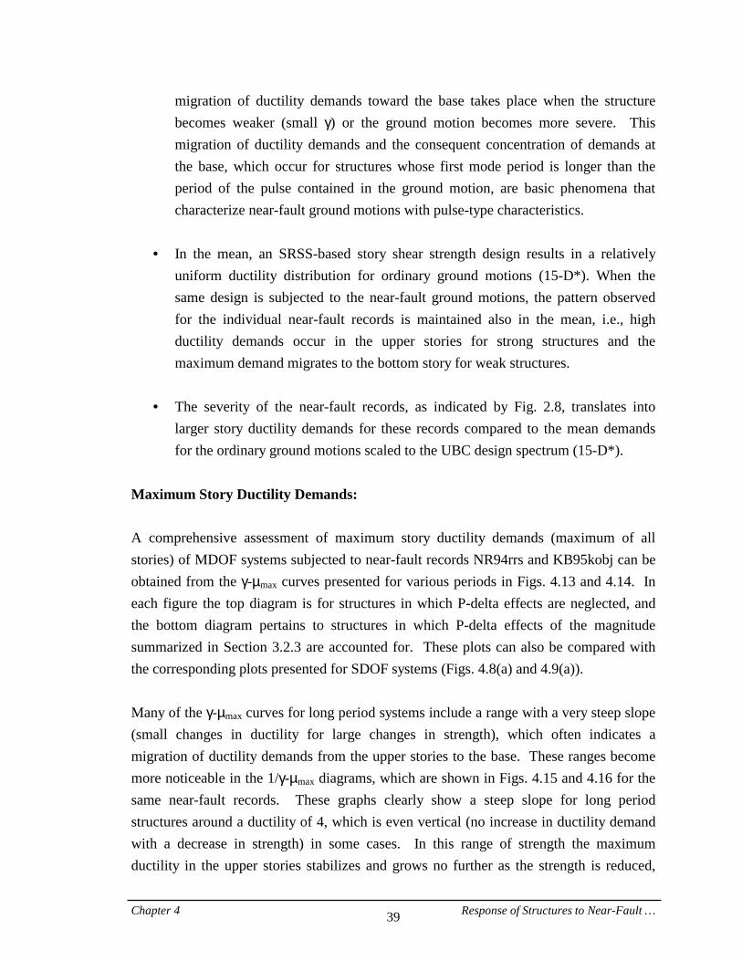
Chapter 4 Response of Structures to Near-Fault … 39
migration of ductility demands toward the base takes place when the structure becomes weaker (small γ) or the ground motion becomes more severe. This migration of ductility demands and the consequent concentration of demands at the base, which occur for structures whose first mode period is longer than the period of the pulse contained in the ground motion, are basic phenomena that characterize near-fault ground motions with pulse-type characteristics.
• = In the mean, an SRSS-based story shear strength design results in a relatively
uniform ductility distribution for ordinary ground motions (15-D*). When the same design is subjected to the near-fault ground motions, the pattern observed for the individual near-fault records is maintained also in the mean, i.e., high ductility demands occur in the upper stories for strong structures and the maximum demand migrates to the bottom story for weak structures.
• = The severity of the near-fault records, as indicated by Fig. 2.8, translates into
larger story ductility demands for these records compared to the mean demands for the ordinary ground motions scaled to the UBC design spectrum (15-D*).
Maximum Story Ductility Demands: A comprehensive assessment of maximum story ductility demands (maximum of all stories) of MDOF systems subjected to near-fault records NR94rrs and KB95kobj can be obtained from the γ-µmax curves presented for various periods in Figs. 4.13 and 4.14. In each figure the top diagram is for structures in which P-delta effects are neglected, and the bottom diagram pertains to structures in which P-delta effects of the magnitude summarized in Section 3.2.3 are accounted for. These plots can also be compared with the corresponding plots presented for SDOF systems (Figs. 4.8(a) and 4.9(a)). Many of the γ-µmax curves for long period systems include a range with a very steep slope (small changes in ductility for large changes in strength), which often indicates a migration of ductility demands from the upper stories to the base. These ranges become more noticeable in the 1/γ-µmax diagrams, which are shown in Figs. 4.15 and 4.16 for the same near-fault records. These graphs clearly show a steep slope for long period structures around a ductility of 4, which is even vertical (no increase in ductility demand with a decrease in strength) in some cases. In this range of strength the maximum ductility in the upper stories stabilizes and grows no further as the strength is reduced,
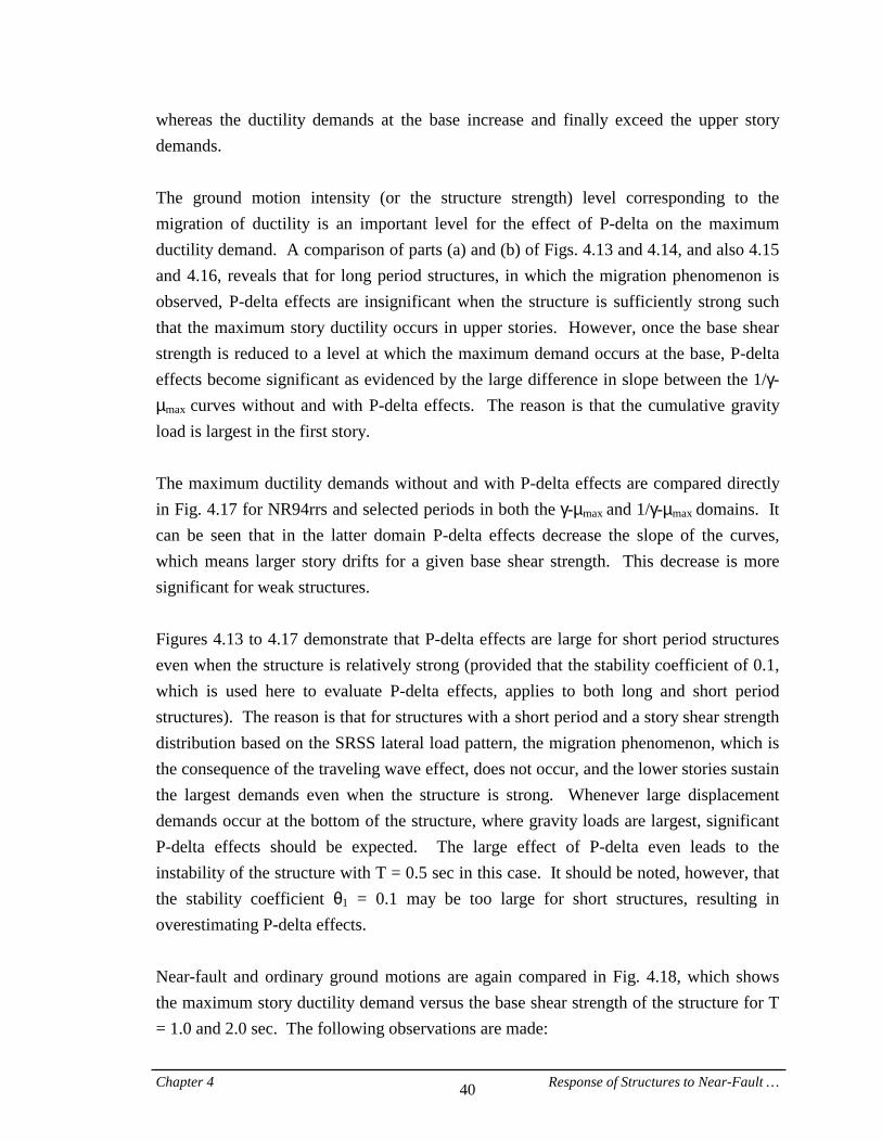
Chapter 4 Response of Structures to Near-Fault … 40
whereas the ductility demands at the base increase and finally exceed the upper story demands. The ground motion intensity (or the structure strength) level corresponding to the migration of ductility is an important level for the effect of P-delta on the maximum ductility demand. A comparison of parts (a) and (b) of Figs. 4.13 and 4.14, and also 4.15 and 4.16, reveals that for long period structures, in which the migration phenomenon is observed, P-delta effects are insignificant when the structure is sufficiently strong such that the maximum story ductility occurs in upper stories. However, once the base shear strength is reduced to a level at which the maximum demand occurs at the base, P-delta effects become significant as evidenced by the large difference in slope between the 1/γ-µmax curves without and with P-delta effects. The reason is that the cumulative gravity load is largest in the first story. The maximum ductility demands without and with P-delta effects are compared directly in Fig. 4.17 for NR94rrs and selected periods in both the γ-µmax and 1/γ-µmax domains. It can be seen that in the latter domain P-delta effects decrease the slope of the curves, which means larger story drifts for a given base shear strength. This decrease is more significant for weak structures. Figures 4.13 to 4.17 demonstrate that P-delta effects are large for short period structures even when the structure is relatively strong (provided that the stability coefficient of 0.1, which is used here to evaluate P-delta effects, applies to both long and short period structures). The reason is that for structures with a short period and a story shear strength distribution based on the SRSS lateral load pattern, the migration phenomenon, which is the consequence of the traveling wave effect, does not occur, and the lower stories sustain the largest demands even when the structure is strong. Whenever large displacement demands occur at the bottom of the structure, where gravity loads are largest, significant P-delta effects should be expected. The large effect of P-delta even leads to the instability of the structure with T = 0.5 sec in this case. It should be noted, however, that the stability coefficient θ1 = 0.1 may be too large for short structures, resulting in overestimating P-delta effects. Near-fault and ordinary ground motions are again compared in Fig. 4.18, which shows the maximum story ductility demand versus the base shear strength of the structure for T = 1.0 and 2.0 sec. The following observations are made:
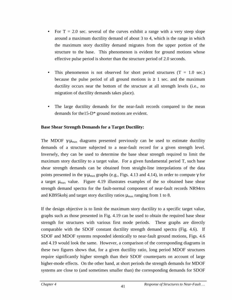
Chapter 4 Response of Structures to Near-Fault … 41
• = For T = 2.0 sec. several of the curves exhibit a range with a very steep slope around a maximum ductility demand of about 3 to 4, which is the range in which the maximum story ductility demand migrates from the upper portion of the structure to the base. This phenomenon is evident for ground motions whose effective pulse period is shorter than the structure period of 2.0 seconds.
• = This phenomenon is not observed for short period structures (T = 1.0 sec.)
because the pulse period of all ground motions is ≥ 1 sec. and the maximum ductility occurs near the bottom of the structure at all strength levels (i.e., no migration of ductility demands takes place).
• = The large ductility demands for the near-fault records compared to the mean
demands for the15-D* ground motions are evident. Base Shear Strength Demands for a Target Ductility: The MDOF γ-µmax diagrams presented previously can be used to estimate ductility demands of a structure subjected to a near-fault record for a given strength level. Inversely, they can be used to determine the base shear strength required to limit the maximum story ductility to a target value. For a given fundamental period T, such base shear strength demands can be obtained from straight-line interpolations of the data points presented in the γ-µmax graphs (e.g., Figs. 4.13 and 4.14), in order to compute γ for a target µmax value. Figure 4.19 illustrates examples of the so obtained base shear strength demand spectra for the fault-normal component of near-fault records NR94rrs and KB95kobj and target story ductility ratios µmax ranging from 1 to 8. If the design objective is to limit the maximum story ductility to a specific target value, graphs such as those presented in Fig. 4.19 can be used to obtain the required base shear strength for structures with various first mode periods. These graphs are directly comparable with the SDOF constant ductility strength demand spectra (Fig. 4.6). If SDOF and MDOF systems responded identically to near-fault ground motions, Figs. 4.6 and 4.19 would look the same. However, a comparison of the corresponding diagrams in these two figures shows that, for a given ductility ratio, long period MDOF structures require significantly higher strength than their SDOF counterparts on account of large higher-mode effects. On the other hand, at short periods the strength demands for MDOF systems are close to (and sometimes smaller than) the corresponding demands for SDOF
Chapter 4 Response of Structures to Near-Fault … 42
systems with the same period. Again, the dividing line between “short” and “long” periods is the period of the pulse contained in the ground motion (1.0 sec. for the NR94rrs record and 0.9 sec. for the KB95kobj record). Strength Demands for Rotated Components: The elastic response spectra of 45° rotated components of near-fault ground motions were evaluated in Section 2.2. It was shown that the elastic response for one of the rotated components is comparable to the response associated with the fault-normal component. In this part of the study the inelastic response of MDOF structures to the rotated components of near-fault records is investigated. MDOF base shear strength demand spectra similar to those presented in Fig. 4.19 can be computed for the rotated components by employing the interpolation scheme discussed earlier. If the strength demand obtained from a rotated component is divided by the corresponding value obtained from the fault-normal component for the same T and µ values, the resulting ratios represent the required base shear strength for the rotated component as a fraction of the strength required for the fault-normal component. Examples of such ratios are illustrated in Figs. 4.20 and 4.21 for the 45° rotated components of near-fault ground motions NR94rrs and KB95kobj. The results indicate that one of the 45° components exposes the structure to strength demands almost as high as those obtained for the fault-normal component. The ratios larger than unity for one of the rotated components of KB95kobj (Fig. 4.21(b)) highlight the intensity of this component. One could argue for a strength reduction factor of about 0.8 for the 45° rotated component, but this argument does not apply consistently. In view of the many uncertainties and unknowns involved in quantifying near-fault effects, it is argued that the emphasis on the fault-normal component as a representative component is justified. 4.3. Displacement Demands for Inelastic Structures 4.3.1. SDOF Inelastic Displacement Demands The elastic displacement spectra of near-fault ground motions were addressed in Chapter 2. This section focuses on a comparison between elastic and inelastic displacement demands for SDOF structures subjected to near-fault records. Examples of this
Chapter 4 Response of Structures to Near-Fault … 43
comparison are provided in Figure 4.22, which presents ratios of inelastic to elastic spectral displacement demands (δin/δel = µ/R) for the fault-normal component of ground motions NR94rrs and KB95kobj. In each case the strength of the inelastic system is selected such that target ductility ratios of µ = 2, 3, 4, 6, and 8 are obtained. The ratios follow patterns observed for ordinary ground motions: in the short period range the inelastic spectral displacements are larger than the elastic ones, and increase with a reduction in strength, whereas the reverse is usually observed in the intermediate period range; in the long period range the inelastic and elastic displacements are close because they both approach the maximum ground displacement. Baez and Miranda (2000) investigated the inelastic to elastic displacement ratios for sets of ordinary and near-fault ground motions, and showed that in the period range from 0.1 to 1.3 sec., the ratios obtained for near-fault records are larger than the ratios obtained for ordinary ground motions, whereas the opposite is true at periods longer than 1.8 sec. They also concluded that the ratios are larger for the fault-normal component of near-fault ground motions compared to the fault-parallel component in the period range from 0.1 to 1.3 sec. 4.3.2. MDOF Inelastic Roof Displacement Demands Information on elastic roof displacement demands for near-fault ground motions was provided in Section 4.1.3. This section addresses the relationship between elastic and inelastic roof displacement demands without P-delta effects. Figure 4.23 illustrates the inelastic roof displacement of MDOF systems with various base shear strength coefficients γ, normalized by their corresponding elastic roof displacement, for ground motions NR94rrs and KB95kobj. The relative values of inelastic to elastic roof displacements generally follow patterns observed for inelastic to elastic spectral displacements (Fig. 4.22). The inelastic roof displacement demands are larger than the elastic ones in the short period range, and become much larger with decreasing period and base shear strength. On the other hand, in the longer period range the reverse is observed, i.e., the inelastic roof displacement demands are smaller than the elastic ones and decrease when the structure becomes weaker.
Chapter 4 Response of Structures to Near-Fault … 44
Summary: The major observation that summarizes the investigations presented in this chapter is that the response of structures to near-fault ground motions with forward directivity has peculiar characteristics that set such motions apart from ordinary ground motions. The response clearly shows pulse-type characteristics that are specific to individual ground motions and strongly depend on the structure period and strength. The effect of the structure period on the response has to be put in perspective with the effective period of the pulse contained in the near-fault ground motion. The identification of the pulse period will be discussed in Chapter 7. In the next chapter, attempts are made to define simple pulse motions whose response attributes are similar to those of near-fault records.
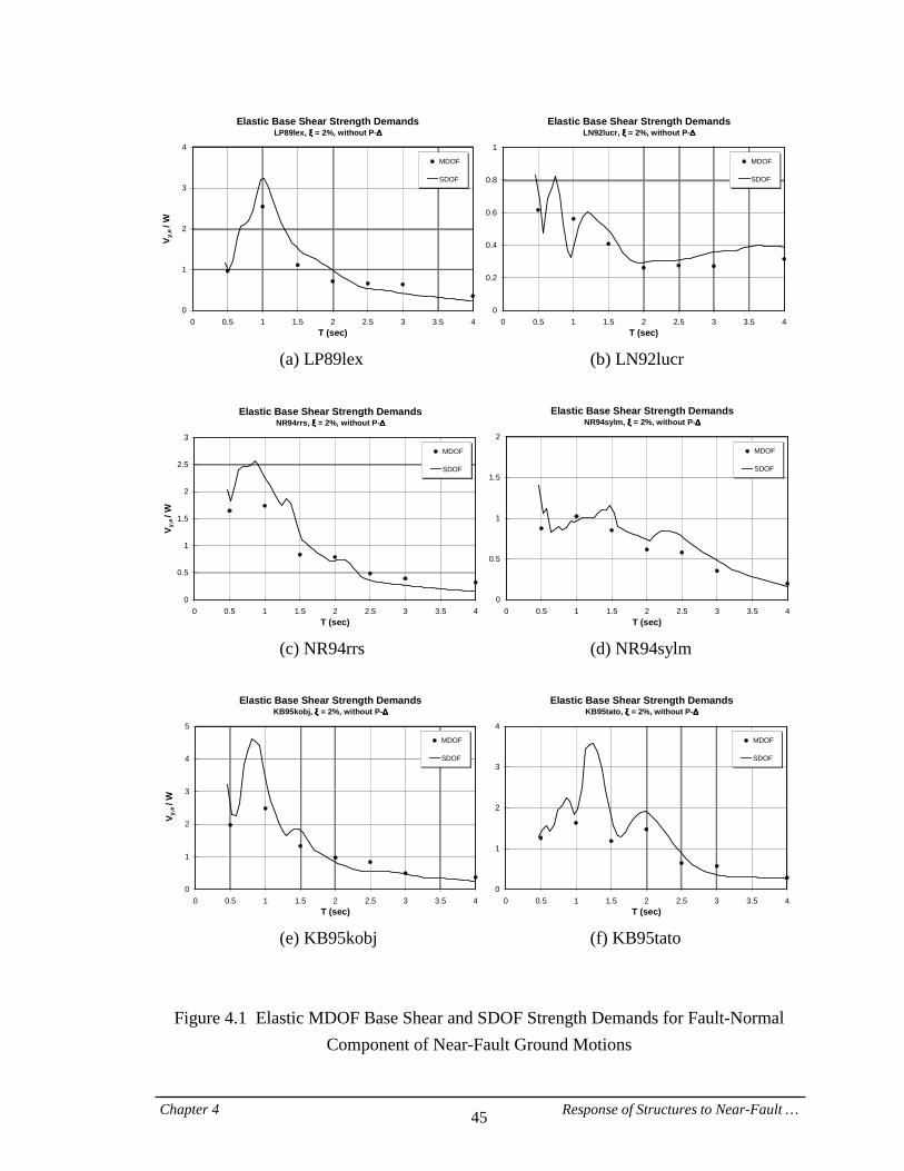
Chapter 4 Response of Structures to Near-Fault … 45
Elastic Base Shear Strength DemandsLP89lex, ξξξξ = 2%, without P-∆∆∆∆
0
1
2
3
4
0 0.5 1 1.5 2 2.5 3 3.5 4T (sec)
V y,e
/ W
MDOF
SDOF
Elastic Base Shear Strength DemandsLN92lucr, ξξξξ = 2%, without P-∆∆∆∆
0
0.2
0.4
0.6
0.8
1
0 0.5 1 1.5 2 2.5 3 3.5 4T (sec)
MDOF
SDOF
(a) LP89lex (b) LN92lucr
Elastic Base Shear Strength Demands
NR94rrs, ξξξξ = 2%, without P-∆∆∆∆
0
0.5
1
1.5
2
2.5
3
0 0.5 1 1.5 2 2.5 3 3.5 4T (sec)
V y,e
/ W
MDOF
SDOF
Elastic Base Shear Strength DemandsNR94sylm, ξξξξ = 2%, without P-∆∆∆∆
0
0.5
1
1.5
2
0 0.5 1 1.5 2 2.5 3 3.5 4T (sec)
MDOF
SDOF
(c) NR94rrs (d) NR94sylm
Elastic Base Shear Strength Demands
KB95kobj, ξξξξ = 2%, without P-∆∆∆∆
0
1
2
3
4
5
0 0.5 1 1.5 2 2.5 3 3.5 4T (sec)
V y,e
/ W
MDOF
SDOF
Elastic Base Shear Strength DemandsKB95tato, ξξξξ = 2%, without P-∆∆∆∆
0
1
2
3
4
0 0.5 1 1.5 2 2.5 3 3.5 4T (sec)
MDOF
SDOF
(e) KB95kobj (f) KB95tato
Figure 4.1 Elastic MDOF Base Shear and SDOF Strength Demands for Fault-Normal Component of Near-Fault Ground Motions
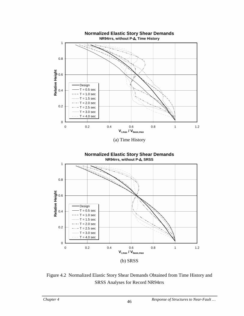
Chapter 4 Response of Structures to Near-Fault … 46
Normalized Elastic Story Shear DemandsNR94rrs, without P-∆∆∆∆, Time History
0
0.2
0.4
0.6
0.8
1
0 0.2 0.4 0.6 0.8 1 1.2Vi,max / Vbase,max
Rel
ativ
e H
eigh
t
DesignT = 0.5 secT = 1.0 secT = 1.5 secT = 2.0 secT = 2.5 secT = 3.0 secT = 4.0 sec
(a) Time History
Normalized Elastic Story Shear Demands
NR94rrs, without P-∆∆∆∆, SRSS
0
0.2
0.4
0.6
0.8
1
0 0.2 0.4 0.6 0.8 1 1.2Vi,max / Vbase,max
Rel
ativ
e H
eigh
t
DesignT = 0.5 secT = 1.0 secT = 1.5 secT = 2.0 secT = 2.5 secT = 3.0 secT = 4.0 sec
(b) SRSS
Figure 4.2 Normalized Elastic Story Shear Demands Obtained from Time History and
SRSS Analyses for Record NR94rrs
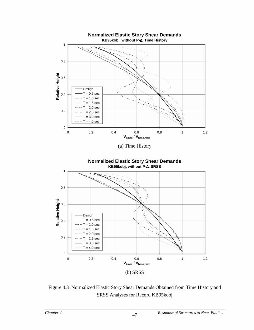
Chapter 4 Response of Structures to Near-Fault … 47
Normalized Elastic Story Shear DemandsKB95kobj, without P-∆∆∆∆, Time History
0
0.2
0.4
0.6
0.8
1
0 0.2 0.4 0.6 0.8 1 1.2Vi,max / Vbase,max
Rel
ativ
e H
eigh
t
DesignT = 0.5 secT = 1.0 secT = 1.5 secT = 2.0 secT = 2.5 secT = 3.0 secT = 4.0 sec
(a) Time History
Normalized Elastic Story Shear Demands
KB95kobj, without P-∆∆∆∆, SRSS
0
0.2
0.4
0.6
0.8
1
0 0.2 0.4 0.6 0.8 1 1.2Vi,max / Vbase,max
Rel
ativ
e H
eigh
t
DesignT = 0.5 secT = 1.0 secT = 1.5 secT = 2.0 secT = 2.5 secT = 3.0 secT = 4.0 sec
(b) SRSS
Figure 4.3 Normalized Elastic Story Shear Demands Obtained from Time History and
SRSS Analyses for Record KB95kobj
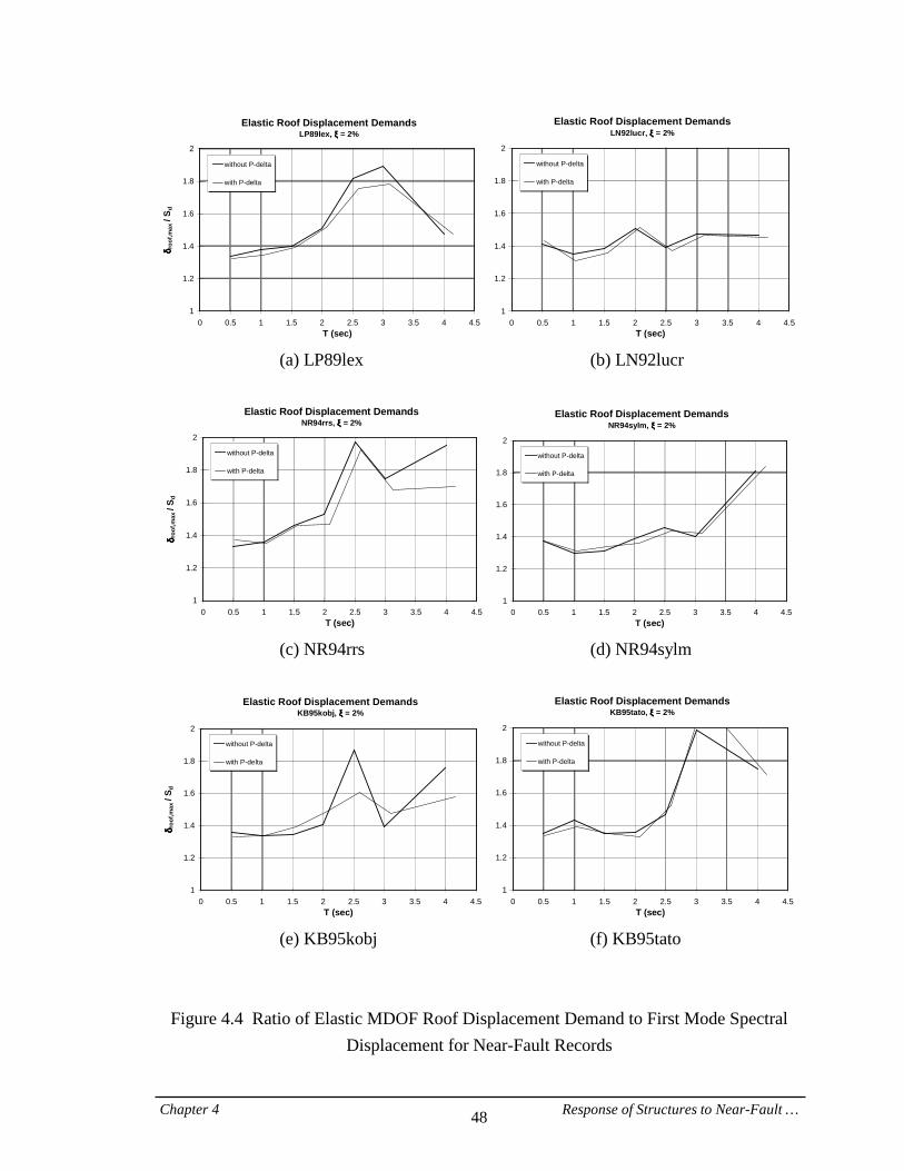
Chapter 4 Response of Structures to Near-Fault … 48
Elastic Roof Displacement DemandsLP89lex, ξξξξ = 2%
1
1.2
1.4
1.6
1.8
2
0 0.5 1 1.5 2 2.5 3 3.5 4 4.5T (sec)
δδ δδ roo
f,max
/ S d
without P-delta
with P-delta
Elastic Roof Displacement DemandsLN92lucr, ξξξξ = 2%
1
1.2
1.4
1.6
1.8
2
0 0.5 1 1.5 2 2.5 3 3.5 4 4.5T (sec)
without P-delta
with P-delta
(a) LP89lex (b) LN92lucr
Elastic Roof Displacement Demands
NR94rrs, ξξξξ = 2%
1
1.2
1.4
1.6
1.8
2
0 0.5 1 1.5 2 2.5 3 3.5 4 4.5T (sec)
δδ δδ roo
f,max
/ S d
without P-delta
with P-delta
Elastic Roof Displacement DemandsNR94sylm, ξξξξ = 2%
1
1.2
1.4
1.6
1.8
2
0 0.5 1 1.5 2 2.5 3 3.5 4 4.5T (sec)
without P-delta
with P-delta
(c) NR94rrs (d) NR94sylm
Elastic Roof Displacement Demands
KB95kobj, ξξξξ = 2%
1
1.2
1.4
1.6
1.8
2
0 0.5 1 1.5 2 2.5 3 3.5 4 4.5T (sec)
δδ δδ roo
f,max
/ S d
without P-delta
with P-delta
Elastic Roof Displacement DemandsKB95tato, ξξξξ = 2%
1
1.2
1.4
1.6
1.8
2
0 0.5 1 1.5 2 2.5 3 3.5 4 4.5T (sec)
without P-delta
with P-delta
(e) KB95kobj (f) KB95tato
Figure 4.4 Ratio of Elastic MDOF Roof Displacement Demand to First Mode Spectral Displacement for Near-Fault Records
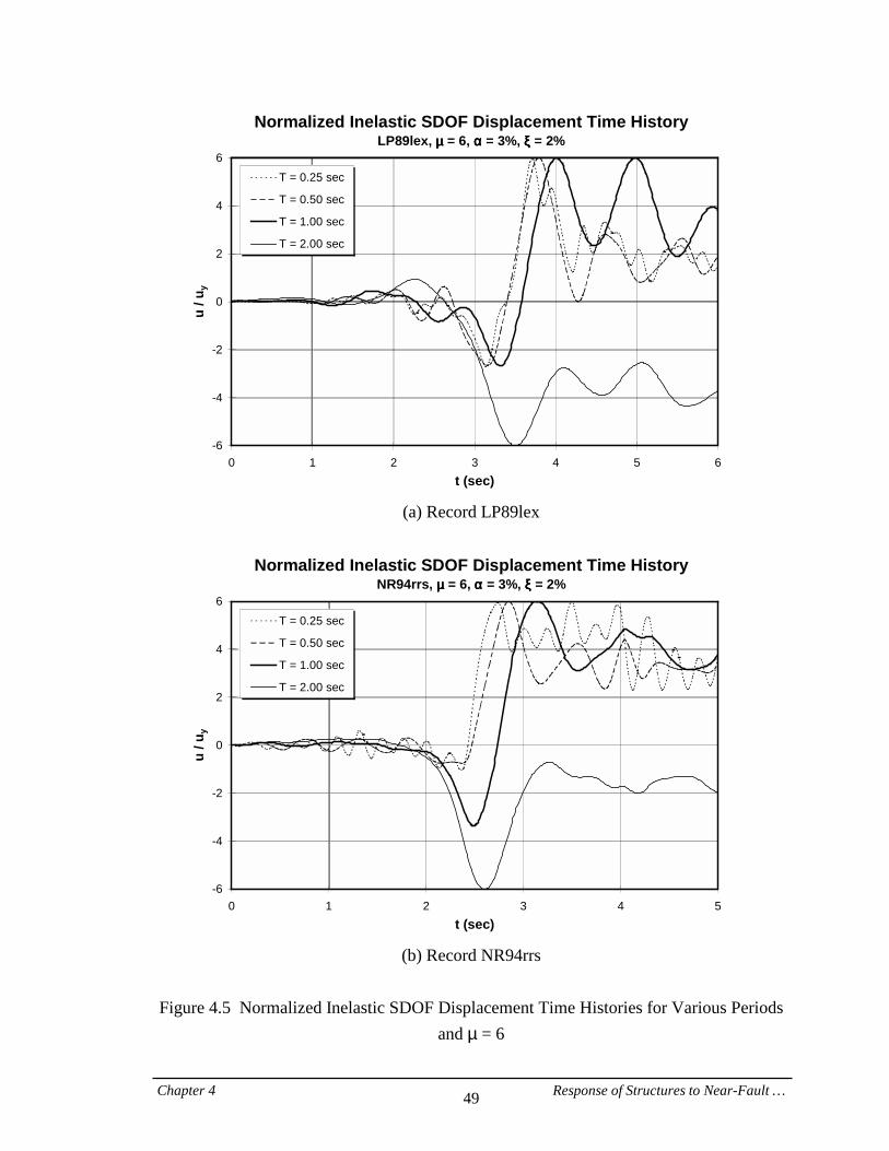
Chapter 4 Response of Structures to Near-Fault … 49
Normalized Inelastic SDOF Displacement Time HistoryLP89lex, µµµµ = 6, αααα = 3%, ξξξξ = 2%
-6
-4
-2
0
2
4
6
0 1 2 3 4 5 6t (sec)
u / u
y
T = 0.25 sec
T = 0.50 sec
T = 1.00 sec
T = 2.00 sec
(a) Record LP89lex
Normalized Inelastic SDOF Displacement Time History
NR94rrs, µµµµ = 6, αααα = 3%, ξξξξ = 2%
-6
-4
-2
0
2
4
6
0 1 2 3 4 5t (sec)
u / u
y
T = 0.25 sec
T = 0.50 sec
T = 1.00 sec
T = 2.00 sec
(b) Record NR94rrs
Figure 4.5 Normalized Inelastic SDOF Displacement Time Histories for Various Periods
and µ = 6
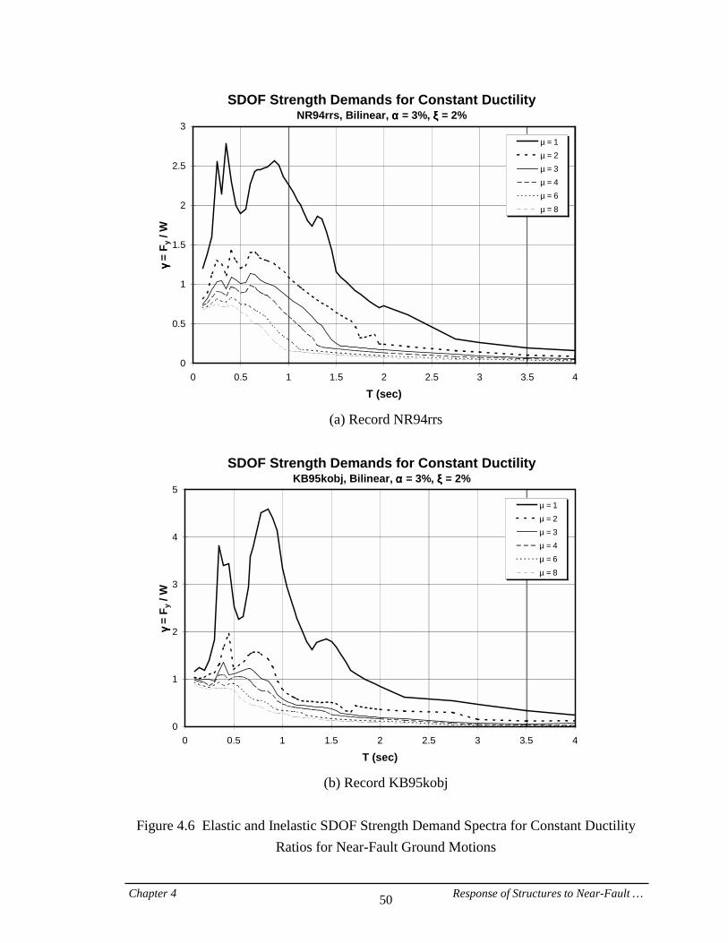
Chapter 4 Response of Structures to Near-Fault … 50
SDOF Strength Demands for Constant DuctilityNR94rrs, Bilinear, αααα = 3%, ξξξξ = 2%
0
0.5
1
1.5
2
2.5
3
0 0.5 1 1.5 2 2.5 3 3.5 4
T (sec)
γγ γγ =
F y /
W
µ===1
µ===2
µ===3
µ===4
µ===6
µ===8
(a) Record NR94rrs
SDOF Strength Demands for Constant Ductility
KB95kobj, Bilinear, αααα = 3%, ξξξξ = 2%
0
1
2
3
4
5
0 0.5 1 1.5 2 2.5 3 3.5 4
T (sec)
γγ γγ =
F y /
W
µ===1
µ===2
µ===3
µ===4
µ===6
µ===8
(b) Record KB95kobj
Figure 4.6 Elastic and Inelastic SDOF Strength Demand Spectra for Constant Ductility
Ratios for Near-Fault Ground Motions
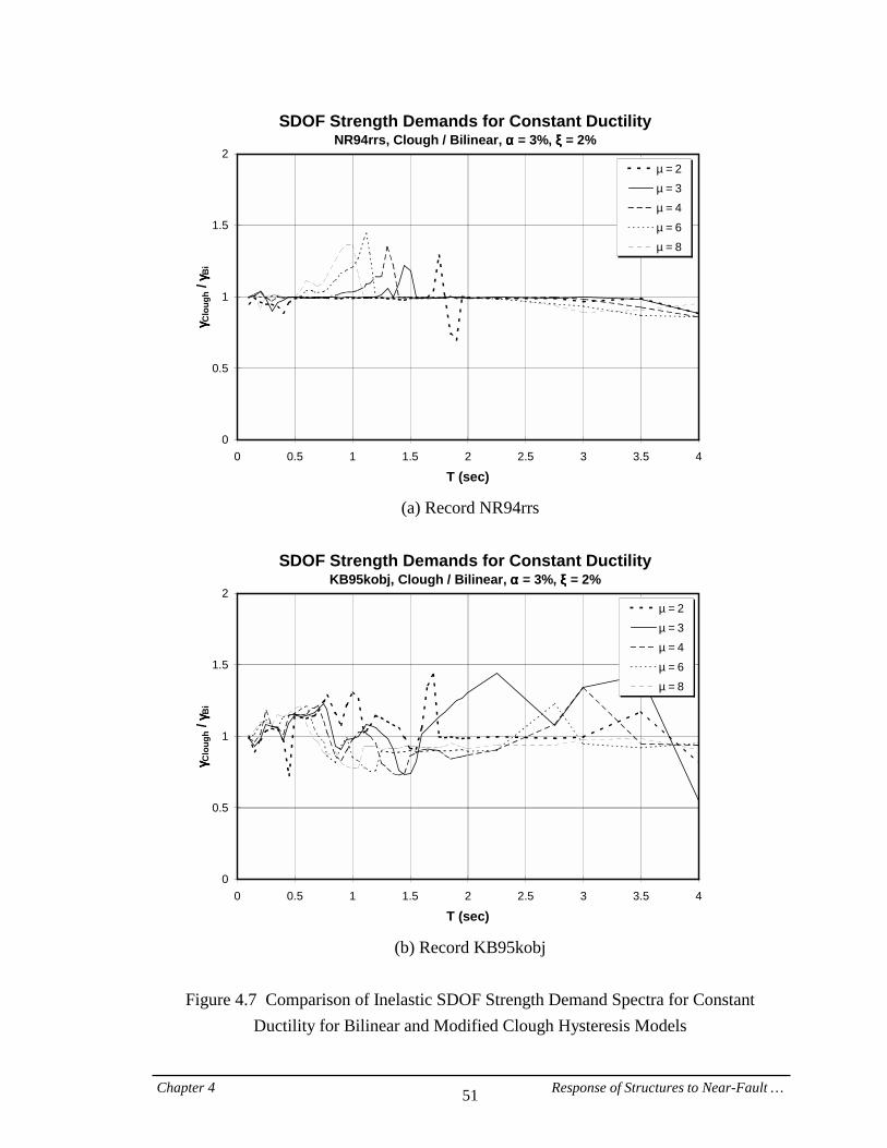
Chapter 4 Response of Structures to Near-Fault … 51
SDOF Strength Demands for Constant DuctilityNR94rrs, Clough / Bilinear, αααα = 3%, ξξξξ = 2%
0
0.5
1
1.5
2
0 0.5 1 1.5 2 2.5 3 3.5 4
T (sec)
γγ γγ Clo
ugh /
γγ γγ Bi
µ===2
µ===3
µ===4
µ===6
µ===8
(a) Record NR94rrs
SDOF Strength Demands for Constant Ductility
KB95kobj, Clough / Bilinear, αααα = 3%, ξξξξ = 2%
0
0.5
1
1.5
2
0 0.5 1 1.5 2 2.5 3 3.5 4
T (sec)
γγ γγ Clo
ugh /
γγ γγ Bi
µ===2
µ===3
µ===4
µ===6
µ===8
(b) Record KB95kobj
Figure 4.7 Comparison of Inelastic SDOF Strength Demand Spectra for Constant
Ductility for Bilinear and Modified Clough Hysteresis Models
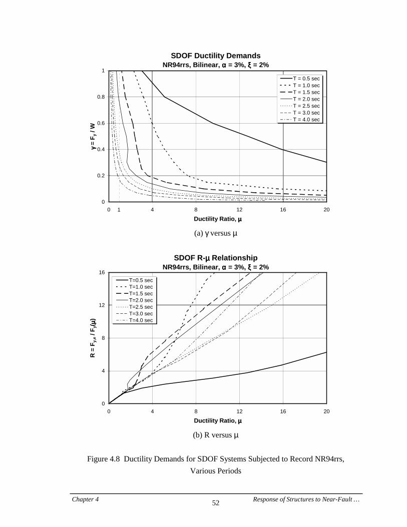
Chapter 4 Response of Structures to Near-Fault … 52
SDOF Ductility DemandsNR94rrs, Bilinear, αααα = 3%, ξξξξ = 2%
0
0.2
0.4
0.6
0.8
1
0 4 8 12 16 20
Ductility Ratio, µµµµ
γγ γγ =
F y /
W
T = 0.5 secT = 1.0 secT = 1.5 secT = 2.0 secT = 2.5 secT = 3.0 secT = 4.0 sec
1
(a) γ versus µ
SDOF R-µµµµ Relationship
NR94rrs, Bilinear, αααα = 3%, ξξξξ = 2%
0
4
8
12
16
0 4 8 12 16 20
Ductility Ratio, µµµµ
R =
Fy,
e / F
y( µµ µµ)
T=0.5 secT=1.0 secT=1.5 secT=2.0 secT=2.5 secT=3.0 secT=4.0 sec
(b) R versus µ=
Figure 4.8 Ductility Demands for SDOF Systems Subjected to Record NR94rrs,
Various Periods
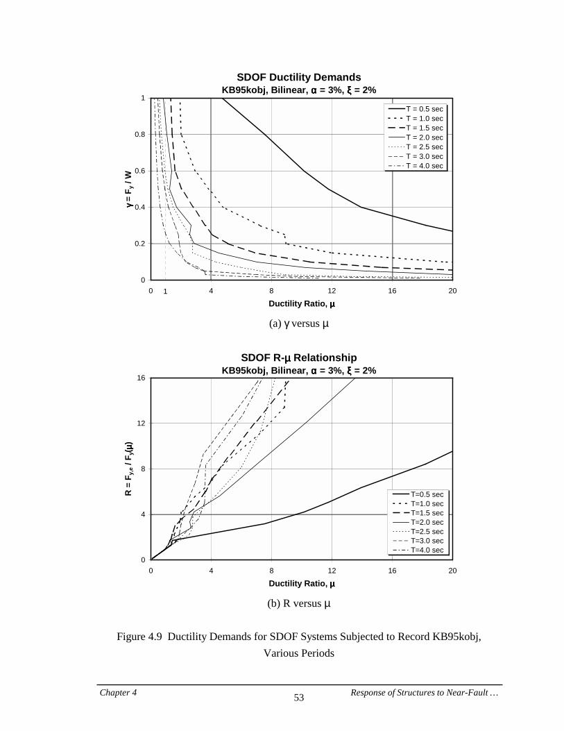
Chapter 4 Response of Structures to Near-Fault … 53
SDOF Ductility DemandsKB95kobj, Bilinear, αααα = 3%, ξξξξ = 2%
0
0.2
0.4
0.6
0.8
1
0 4 8 12 16 20
Ductility Ratio, µµµµ
γγ γγ =
F y /
W
T = 0.5 secT = 1.0 secT = 1.5 secT = 2.0 secT = 2.5 secT = 3.0 secT = 4.0 sec
1
(a)=γ versus µ
SDOF R-µµµµ Relationship
KB95kobj, Bilinear, αααα = 3%, ξξξξ = 2%
0
4
8
12
16
0 4 8 12 16 20
Ductility Ratio, µµµµ
R =
Fy,
e / F
y( µµ µµ)
T=0.5 secT=1.0 secT=1.5 secT=2.0 secT=2.5 secT=3.0 secT=4.0 sec
(b) R versus µ=
=
Figure 4.9 Ductility Demands for SDOF Systems Subjected to Record KB95kobj, Various Periods
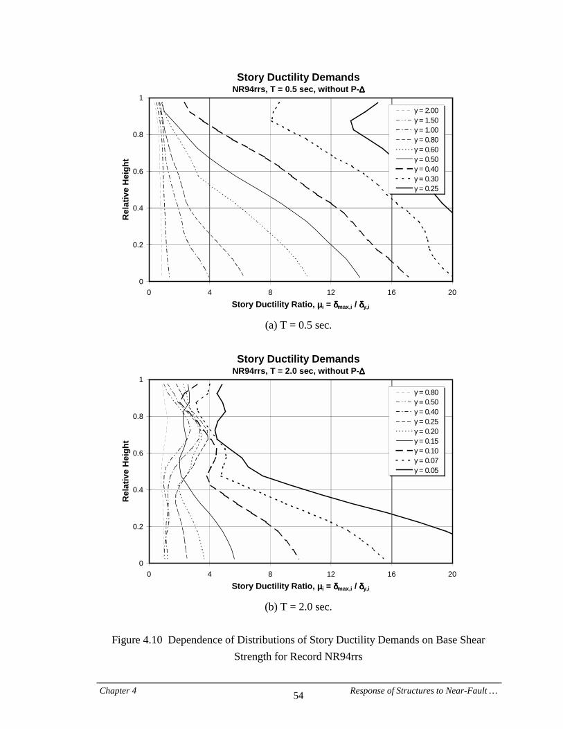
Chapter 4 Response of Structures to Near-Fault … 54
Story Ductility DemandsNR94rrs, T = 0.5 sec, without P-∆∆∆∆
0
0.2
0.4
0.6
0.8
1
0 4 8 12 16 20Story Ductility Ratio, µµµµi = δδδδmax,i / δδδδy,i
Rel
ativ
e H
eigh
t
γ===2.00γ===1.50γ===1.00γ===0.80γ===0.60γ===0.50γ===0.40γ===0.30γ===0.25
(a) T = 0.5 sec.
Story Ductility Demands
NR94rrs, T = 2.0 sec, without P-∆∆∆∆
0
0.2
0.4
0.6
0.8
1
0 4 8 12 16 20Story Ductility Ratio, µµµµi = δδδδmax,i / δδδδy,i
Rel
ativ
e H
eigh
t
γ===0.80γ===0.50γ===0.40γ===0.25γ===0.20γ===0.15γ===0.10γ===0.07γ===0.05
(b) T = 2.0 sec.
Figure 4.10 Dependence of Distributions of Story Ductility Demands on Base Shear
Strength for Record NR94rrs
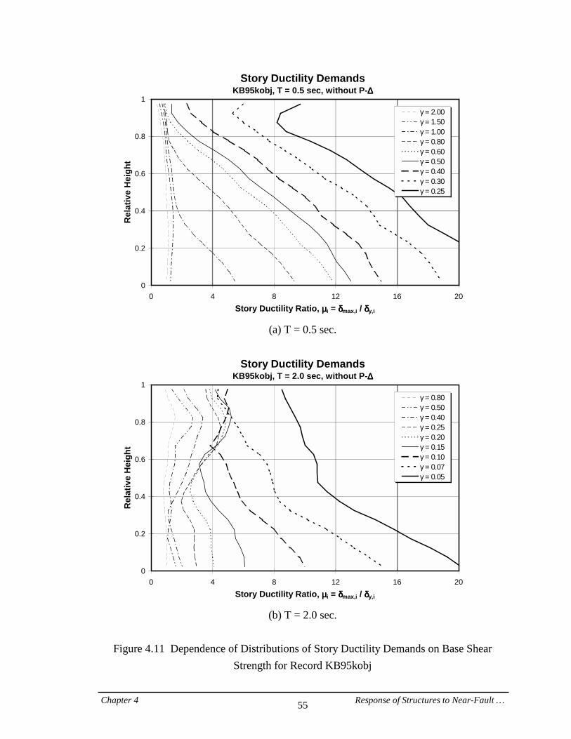
Chapter 4 Response of Structures to Near-Fault … 55
Story Ductility DemandsKB95kobj, T = 0.5 sec, without P-∆∆∆∆
0
0.2
0.4
0.6
0.8
1
0 4 8 12 16 20Story Ductility Ratio, µµµµi = δδδδmax,i / δδδδy,i
Rel
ativ
e H
eigh
t
γ===2.00γ===1.50γ===1.00γ===0.80γ===0.60γ===0.50γ===0.40γ===0.30γ===0.25
(a) T = 0.5 sec.
Story Ductility Demands
KB95kobj, T = 2.0 sec, without P-∆∆∆∆
0
0.2
0.4
0.6
0.8
1
0 4 8 12 16 20Story Ductility Ratio, µµµµi = δδδδmax,i / δδδδy,i
Rel
ativ
e H
eigh
t
γ===0.80γ===0.50γ===0.40γ===0.25γ===0.20γ===0.15γ===0.10γ===0.07γ===0.05
(b) T = 2.0 sec.
Figure 4.11 Dependence of Distributions of Story Ductility Demands on Base Shear
Strength for Record KB95kobj
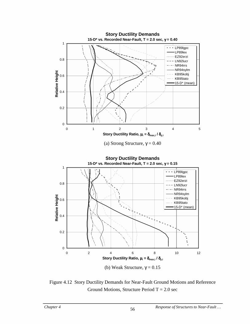
Chapter 4 Response of Structures to Near-Fault … 56
Story Ductility Demands15-D* vs. Recorded Near-Fault, T = 2.0 sec, γγγγ = 0.40
0
0.2
0.4
0.6
0.8
1
0 1 2 3 4 5Story Ductility Ratio, µµµµi = δδδδmax,i / δδδδy,i
Rel
ativ
e H
eigh
t
LP89lgpcLP89lexEZ92erziLN92lucrNR94rrsNR94sylmKB95kobjKB95tato15-D* (mean)
(a) Strong Structure, γ = 0.40
Story Ductility Demands
15-D* vs. Recorded Near-Fault, T = 2.0 sec, γγγγ = 0.15
0
0.2
0.4
0.6
0.8
1
0 2 4 6 8 10 12Story Ductility Ratio, µµµµi = δδδδmax,i / δδδδy,i
Rel
ativ
e H
eigh
t
LP89lgpcLP89lexEZ92erziLN92lucrNR94rrsNR94sylmKB95kobjKB95tato15-D* (mean)
(b) Weak Structure, γ = 0.15
Figure 4.12 Story Ductility Demands for Near-Fault Ground Motions and Reference
Ground Motions, Structure Period T = 2.0 sec
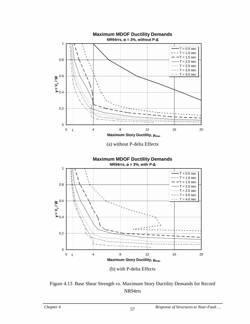
Chapter 4 Response of Structures to Near-Fault … 57
Maximum MDOF Ductility DemandsNR94rrs, αααα = 3%, without P-∆∆∆∆
0
0.2
0.4
0.6
0.8
1
0 4 8 12 16 20Maximum Story Ductility, µµµµmax
γγ γγ == ===
V y /
W
T = 0.5 secT = 1.0 secT = 1.5 secT = 2.0 secT = 2.5 secT = 3.0 secT = 4.0 sec
1
(a) without P-delta Effects
Maximum MDOF Ductility Demands
NR94rrs, αααα = 3%, with P-∆∆∆∆
0
0.2
0.4
0.6
0.8
1
0 4 8 12 16 20Maximum Story Ductility, µµµµmax
γγ γγ == ===
V y /
W
T = 0.5 secT = 1.0 secT = 1.5 secT = 2.0 secT = 2.5 secT = 3.0 secT = 4.0 sec
1
(b) with P-delta Effects
Figure 4.13 Base Shear Strength vs. Maximum Story Ductility Demands for Record
NR94rrs
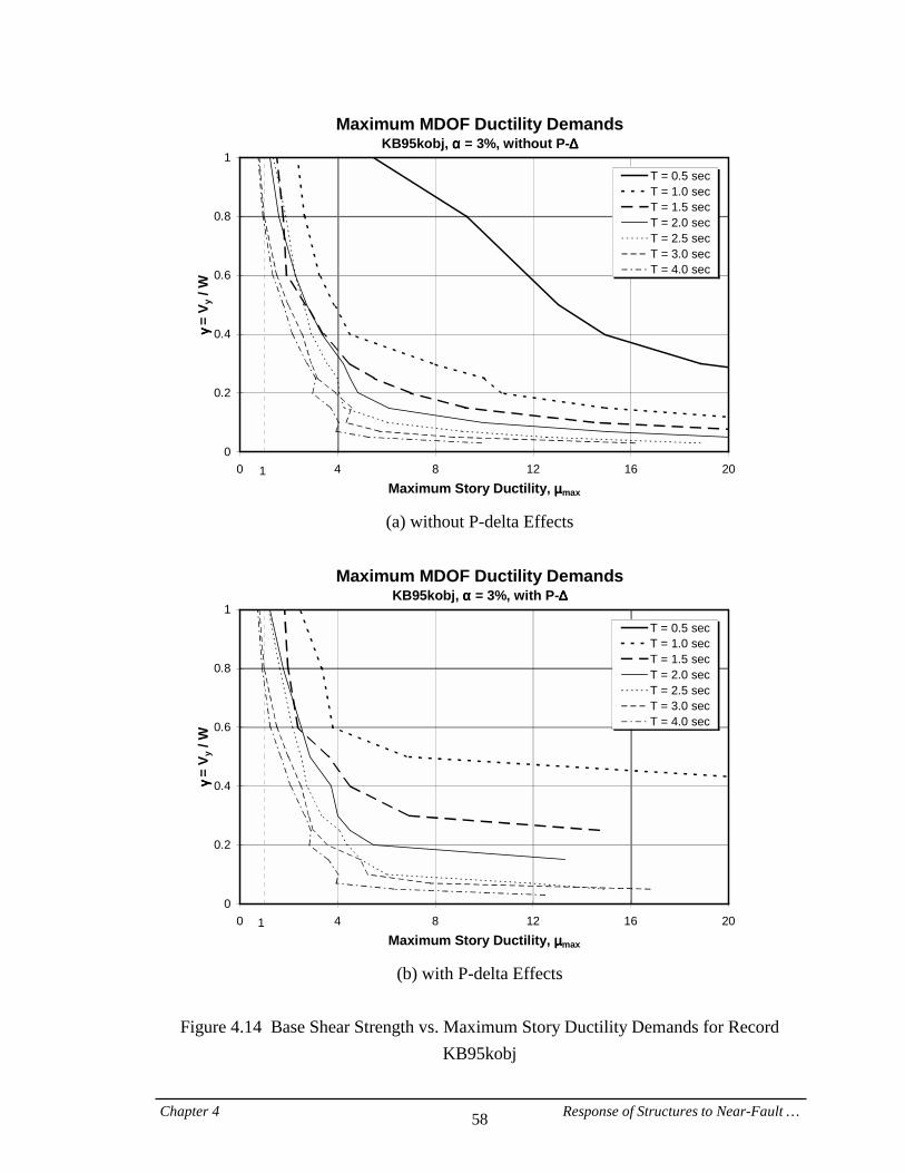
Chapter 4 Response of Structures to Near-Fault … 58
Maximum MDOF Ductility DemandsKB95kobj, αααα = 3%, without P-∆∆∆∆
0
0.2
0.4
0.6
0.8
1
0 4 8 12 16 20Maximum Story Ductility, µµµµmax
γγ γγ == ===
V y /
W
T = 0.5 secT = 1.0 secT = 1.5 secT = 2.0 secT = 2.5 secT = 3.0 secT = 4.0 sec
1
(a) without P-delta Effects
Maximum MDOF Ductility Demands
KB95kobj, αααα = 3%, with P-∆∆∆∆
0
0.2
0.4
0.6
0.8
1
0 4 8 12 16 20Maximum Story Ductility, µµµµmax
γγ γγ == ===
V y /
W
T = 0.5 secT = 1.0 secT = 1.5 secT = 2.0 secT = 2.5 secT = 3.0 secT = 4.0 sec
1
(b) with P-delta Effects
Figure 4.14 Base Shear Strength vs. Maximum Story Ductility Demands for Record
KB95kobj
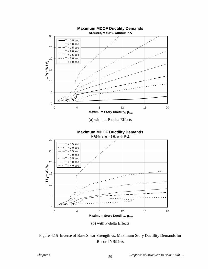
Chapter 4 Response of Structures to Near-Fault … 59
Maximum MDOF Ductility DemandsNR94rrs, αααα = 3%, without P-∆∆∆∆
0
5
10
15
20
25
30
0 4 8 12 16 20Maximum Story Ductility, µµµµmax
1 / γγ γγ=
= =
=
= W
/ V y
T = 0.5 secT = 1.0 secT = 1.5 secT = 2.0 secT = 2.5 secT = 3.0 secT = 4.0 sec
(a) without P-delta Effects
Maximum MDOF Ductility Demands
NR94rrs, αααα = 3%, with P-∆∆∆∆
0
5
10
15
20
25
30
0 4 8 12 16 20Maximum Story Ductility, µµµµmax
1 / γγ γγ=
= =
=
= W
/ V y
T = 0.5 secT = 1.0 secT = 1.5 secT = 2.0 secT = 2.5 secT = 3.0 secT = 4.0 sec
(b) with P-delta Effects
Figure 4.15 Inverse of Base Shear Strength vs. Maximum Story Ductility Demands for
Record NR94rrs

Chapter 4 Response of Structures to Near-Fault … 60
Maximum MDOF Ductility DemandsKB95kobj, αααα = 3%, without P-∆∆∆∆
0
5
10
15
20
25
30
0 4 8 12 16 20Maximum Story Ductility, µµµµmax
1 / γγ γγ=
= =
=
= W
/ V y
T = 0.5 secT = 1.0 secT = 1.5 secT = 2.0 secT = 2.5 secT = 3.0 secT = 4.0 sec
(a) without P-delta Effects
Maximum MDOF Ductility Demands
KB95kobj, αααα = 3%, with P-∆∆∆∆
0
5
10
15
20
25
30
0 4 8 12 16 20Maximum Story Ductility, µµµµmax
1 / γγ γγ=
= =
=
= W
/ V y
T = 0.5 secT = 1.0 secT = 1.5 secT = 2.0 secT = 2.5 secT = 3.0 secT = 4.0 sec
(b) with P-delta Effects
Figure 4.16 Inverse of Base Shear Strength vs. Maximum Story Ductility Demands for
Record KB95kobj
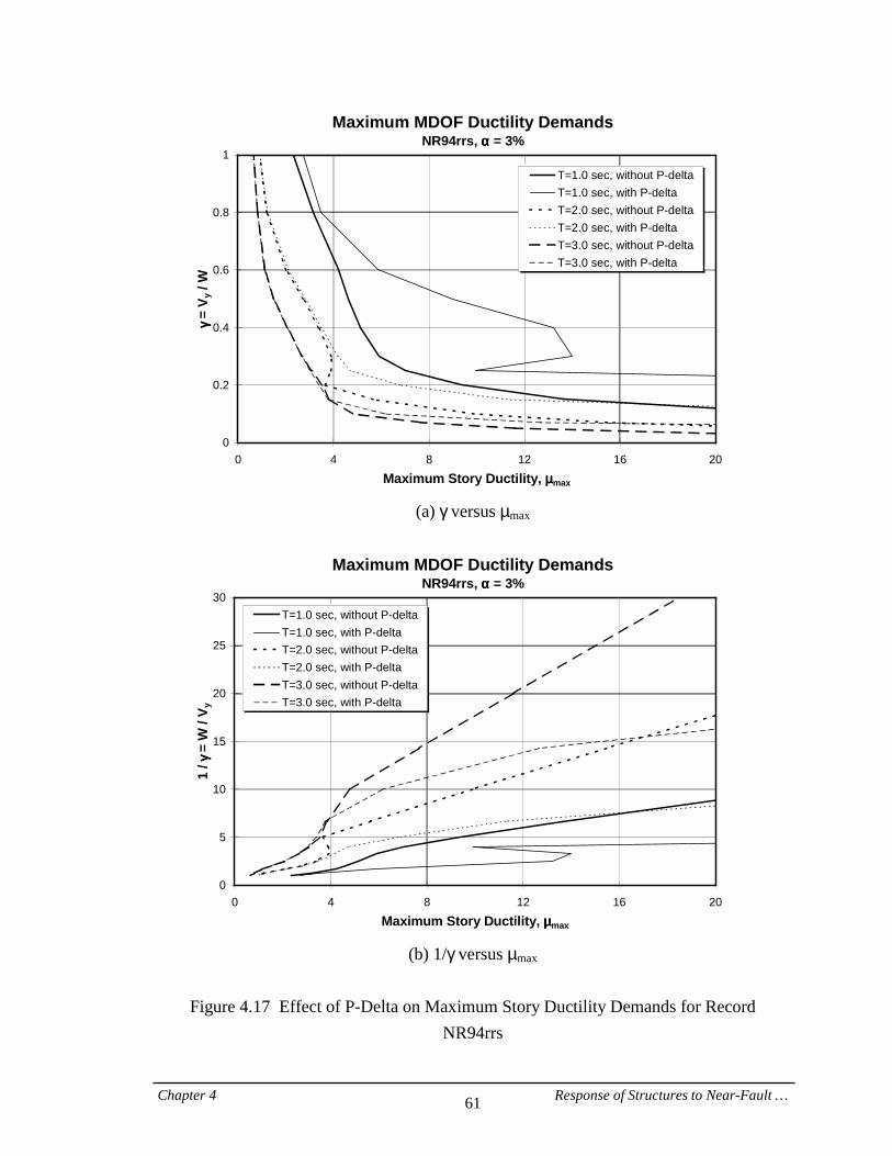
Chapter 4 Response of Structures to Near-Fault … 61
Maximum MDOF Ductility DemandsNR94rrs, αααα = 3%
0
0.2
0.4
0.6
0.8
1
0 4 8 12 16 20Maximum Story Ductility, µµµµmax
γγ γγ == ===
V y /
W
T=1.0 sec, without P-deltaT=1.0 sec, with P-deltaT=2.0 sec, without P-deltaT=2.0 sec, with P-deltaT=3.0 sec, without P-deltaT=3.0 sec, with P-delta
(a) γ versus µmax
Maximum MDOF Ductility Demands
NR94rrs, αααα = 3%
0
5
10
15
20
25
30
0 4 8 12 16 20Maximum Story Ductility, µµµµmax
1 / γγ γγ=
= =
=
= W
/ V y
T=1.0 sec, without P-deltaT=1.0 sec, with P-deltaT=2.0 sec, without P-deltaT=2.0 sec, with P-deltaT=3.0 sec, without P-deltaT=3.0 sec, with P-delta
(b) 1/γ versus µmax
Figure 4.17 Effect of P-Delta on Maximum Story Ductility Demands for Record
NR94rrs
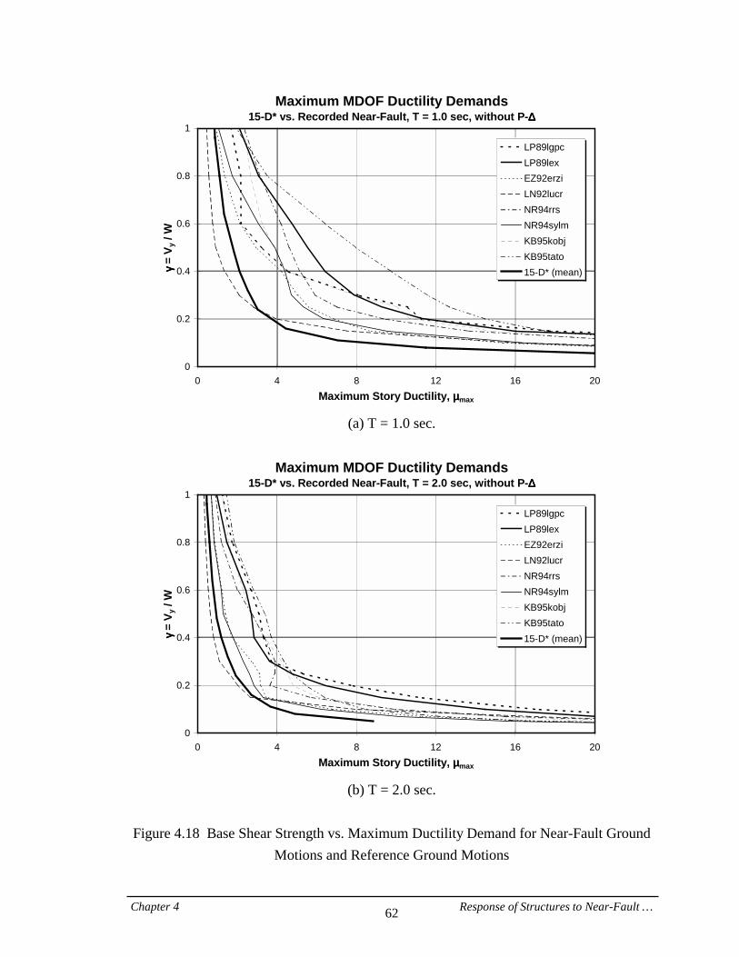
Chapter 4 Response of Structures to Near-Fault … 62
Maximum MDOF Ductility Demands 15-D* vs. Recorded Near-Fault, T = 1.0 sec, without P-∆∆∆∆
0
0.2
0.4
0.6
0.8
1
0 4 8 12 16 20Maximum Story Ductility, µµµµmax
γγ γγ =
V y /
W
LP89lgpcLP89lexEZ92erziLN92lucrNR94rrsNR94sylmKB95kobjKB95tato15-D* (mean)
(a) T = 1.0 sec.
Maximum MDOF Ductility Demands
15-D* vs. Recorded Near-Fault, T = 2.0 sec, without P-∆∆∆∆
0
0.2
0.4
0.6
0.8
1
0 4 8 12 16 20Maximum Story Ductility, µµµµmax
γγ γγ =
V y /
W
LP89lgpcLP89lexEZ92erziLN92lucrNR94rrsNR94sylmKB95kobjKB95tato15-D* (mean)
(b) T = 2.0 sec.
Figure 4.18 Base Shear Strength vs. Maximum Ductility Demand for Near-Fault Ground
Motions and Reference Ground Motions

Chapter 4 Response of Structures to Near-Fault … 63
MDOF Strength Demands for Constant DuctilityNR94rrs, Fault-Normal, ξξξξ = 2%, without P-∆∆∆∆
0
0.5
1
1.5
2
2.5
3
0 0.5 1 1.5 2 2.5 3
T (sec)
γγ γγ =
V y /
W
µ===1µ===2µ===3µ===4µ===6µ===8
(a) Record NR94rrs
MDOF Strength Demands for Constant Ductility
KB95kobj, Fault-Normal, ξξξξ = 2%, without P-∆∆∆∆
0
1
2
3
4
5
0 0.5 1 1.5 2 2.5 3
T (sec)
γγ γγ =
V y /
W
µ===1µ===2µ===3µ===4µ===6µ===8
(b) Record KB95kobj
Figure 4.19 MDOF Base Shear Strength Demand Spectra for Target Maximum Story
Ductility, Near-Fault Ground Motions
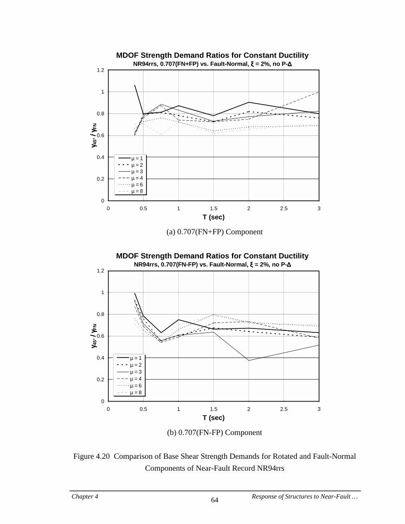
Chapter 4 Response of Structures to Near-Fault … 64
MDOF Strength Demand Ratios for Constant DuctilityNR94rrs, 0.707(FN+FP) vs. Fault-Normal, ξξξξ = 2%, no P-∆∆∆∆
0
0.2
0.4
0.6
0.8
1
1.2
0 0.5 1 1.5 2 2.5 3
T (sec)
γγ γγ 45°=
= =
=
// // == == γγ γγFN
µ===1µ===2µ===3µ===4µ===6µ===8
(a) 0.707(FN+FP) Component
MDOF Strength Demand Ratios for Constant Ductility
NR94rrs, 0.707(FN-FP) vs. Fault-Normal, ξξξξ = 2%, no P-∆∆∆∆
0
0.2
0.4
0.6
0.8
1
1.2
0 0.5 1 1.5 2 2.5 3
T (sec)
γγ γγ 45°=
= =
=
// // == == γγ γγFN
µ===1µ===2µ===3µ===4µ===6µ===8
(b) 0.707(FN-FP) Component
Figure 4.20 Comparison of Base Shear Strength Demands for Rotated and Fault-Normal
Components of Near-Fault Record NR94rrs
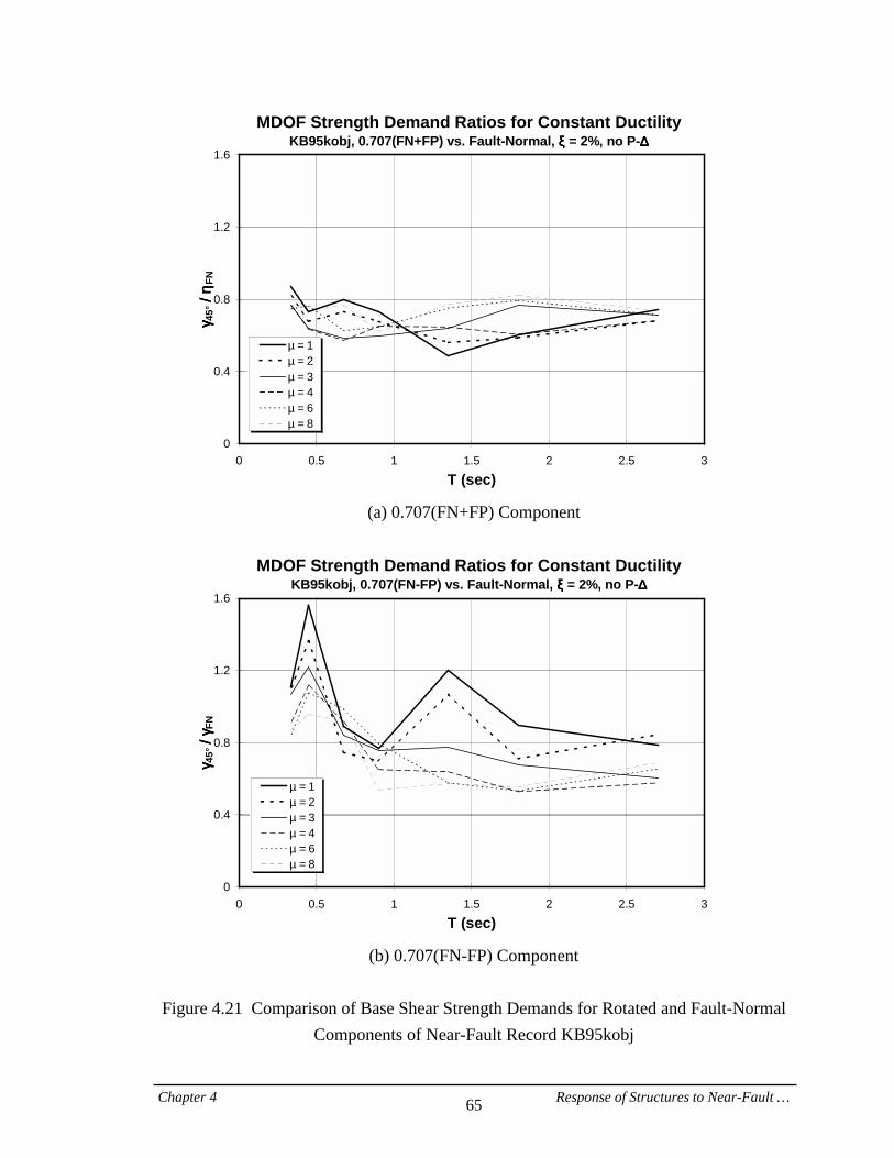
Chapter 4 Response of Structures to Near-Fault … 65
MDOF Strength Demand Ratios for Constant DuctilityKB95kobj, 0.707(FN+FP) vs. Fault-Normal, ξξξξ = 2%, no P-∆∆∆∆
0
0.4
0.8
1.2
1.6
0 0.5 1 1.5 2 2.5 3
T (sec)
γγ γγ 45°=
= =
=
// // == == ηη ηηFN
µ===1µ===2µ===3µ===4µ===6µ===8
(a) 0.707(FN+FP) Component
MDOF Strength Demand Ratios for Constant Ductility
KB95kobj, 0.707(FN-FP) vs. Fault-Normal, ξξξξ = 2%, no P-∆∆∆∆
0
0.4
0.8
1.2
1.6
0 0.5 1 1.5 2 2.5 3
T (sec)
γγ γγ 45°=
= =
=
// // == == γγ γγFN
µ===1µ===2µ===3µ===4µ===6µ===8
(b) 0.707(FN-FP) Component
Figure 4.21 Comparison of Base Shear Strength Demands for Rotated and Fault-Normal
Components of Near-Fault Record KB95kobj
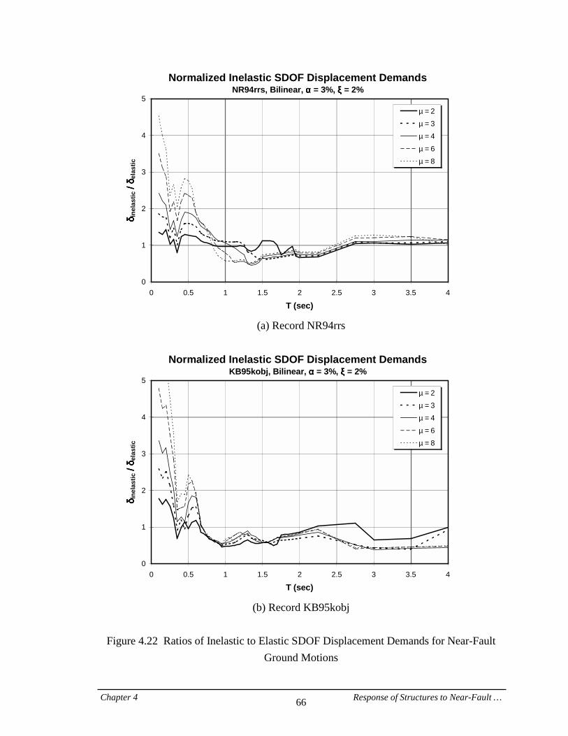
Chapter 4 Response of Structures to Near-Fault … 66
Normalized Inelastic SDOF Displacement DemandsNR94rrs, Bilinear, αααα = 3%, ξξξξ = 2%
0
1
2
3
4
5
0 0.5 1 1.5 2 2.5 3 3.5 4
T (sec)
δδ δδ ine
last
ic=
= =
=
// // == == δδ δδel
astic
µ===2
µ===3
µ===4
µ===6
µ===8
(a) Record NR94rrs
Normalized Inelastic SDOF Displacement Demands
KB95kobj, Bilinear, αααα = 3%, ξξξξ = 2%
0
1
2
3
4
5
0 0.5 1 1.5 2 2.5 3 3.5 4
T (sec)
δδ δδ ine
last
ic=
= =
=
// // == == δδ δδel
astic
µ===2
µ===3
µ===4
µ===6
µ===8
(b) Record KB95kobj
Figure 4.22 Ratios of Inelastic to Elastic SDOF Displacement Demands for Near-Fault
Ground Motions
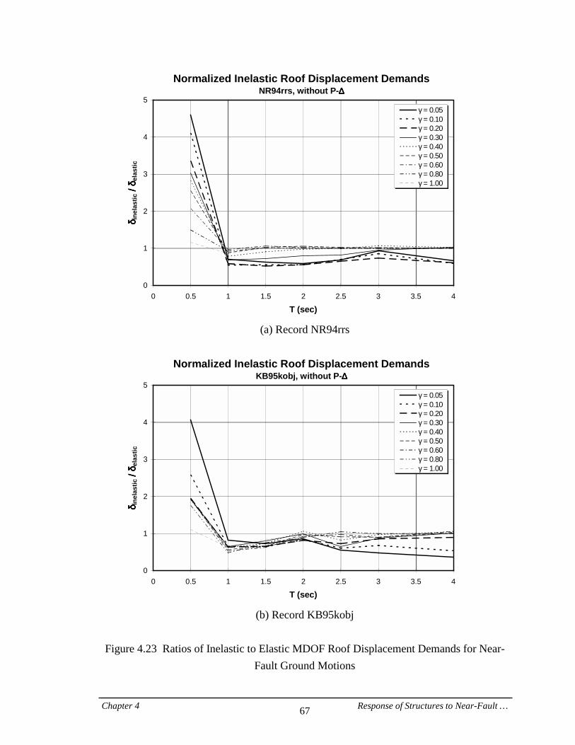
Chapter 4 Response of Structures to Near-Fault … 67
Normalized Inelastic Roof Displacement DemandsNR94rrs, without P-∆∆∆∆
0
1
2
3
4
5
0 0.5 1 1.5 2 2.5 3 3.5 4
T (sec)
δδ δδ ine
last
ic=
= =
=
// // == == δδ δδel
astic
γ===0.05γ===0.10γ===0.20γ===0.30γ===0.40γ===0.50γ===0.60γ===0.80γ===1.00
(a) Record NR94rrs
Normalized Inelastic Roof Displacement Demands
KB95kobj, without P-∆∆∆∆
0
1
2
3
4
5
0 0.5 1 1.5 2 2.5 3 3.5 4
T (sec)
δδ δδ ine
last
ic=
= =
=
// // == == δδ δδel
astic
γ===0.05γ===0.10γ===0.20γ===0.30γ===0.40γ===0.50γ===0.60γ===0.80γ===1.00
(b) Record KB95kobj
Figure 4.23 Ratios of Inelastic to Elastic MDOF Roof Displacement Demands for Near-
Fault Ground Motions
Chapter 5 Pulse-Type Seismic Input 68
CHAPTER 5
PULSE-TYPE SEISMIC INPUT
As discussed in Chapters 2 and 4, pulse-type characteristics are discernible in both the ground motion time history traces and the response of structures to near-fault ground motions with forward directivity. It was also shown that near-fault ground motions come in large variations, which make a consistent evaluation of near-fault effects difficult and cumbersome. If simple pulse models can be found that represent near-fault ground motions with reasonable accuracy, the process of design or response evaluation will be significantly facilitated. Furthermore, the study of simple pulses along with real ground motions provides a more transparent picture of near-fault response properties, and leads to a better understanding of the near-fault phenomena. The objective of this part of the study is to introduce such simplified representations of near-fault ground motions. Various pulse shapes and their spectral values are evaluated. Three basic pulse shapes are utilized for this purpose. Other variations are also investigated in addition to the three basic pulses. A comprehensive evaluation of the response of structures to several of these pulse-type input motions is presented in the next chapter. 5.1. Historical Perspective The study of the dynamic response of structures to impulsive loading dates back to the mid 20th century, when input pulses were first utilized to model the impact forces imposed by bomb blasts. Biggs (1964) evaluated the response of elastic and inelastic SDOF systems to one-sided force pulses of various shapes, i.e., rectangular, triangular and ramp-like pulses. He observed that for each pulse shape, the maximum elastic response is a function of the pulse intensity and the td/T ratio, where td is the duration of the pulse and T is the natural period of the system. For undamped elastic systems
Chapter 5 Pulse-Type Seismic Input 69
subjected to the one-sided force pulses, the displacement response factor (maximum dynamic displacement normalized by static displacement) does not exceed 2.0. For elasto-plastic systems, he illustrated the dependence of the ductility demand on the td/T ratio and the strength of the system relative to the intensity of the input pulse. The response of elastic SDOF systems to a half-cycle sinusoidal force pulse is discussed in Chopra (1995). Chopra demonstrated that the effect of damping on the maximum response to pulse-type forces is not significant unless the system is highly damped. The reason is that the energy dissipated by damping is small when the system is subjected to pulse-type excitations with short duration. For the sinusoidal pulse the displacement response factor is more sensitive to the damping ratio when the pulse duration is shorter than the natural period of the system. Simple pulse shapes have been used in the literature also to represent earthquake ground motions (Veletsos et al., 1965). In the past, when ground motion records were scarce and an evaluation of dynamic response was computationally expensive and time consuming, simple pulses were very useful. Veletsos et al. (1965) presented elastic response spectra for half- and full-cycle sinusoidal pulses of ground velocity. Their plots illustrated the spectra for various damping ratios, indicating that the largest effect of damping is obtained in the medium period range. They also evaluated inelastic strength demand spectra for various target ductility ratios and an undamped elasto-plastic system subjected to a half-cycle ground velocity pulse. The full-cycle velocity pulse was used in their study to represent the Eureka ground motion, recorded in the California earthquake of December 21, 1954. The results of their pulse study are in general agreement with the response of SDOF systems to the pulses introduced in this chapter. As discussed in the next section, triangular velocity pulses, whose acceleration time histories are represented by square waves, are utilized primarily in this study. The effect of rise time will be investigated later by studying triangular acceleration pulses. 5.2. Basic Pulse Shapes Used in this Study The following three pulses (Figs. 5.1 to 5.3) are used as the basis for a representation of the impulsive characteristics of near-fault ground motions. These pulses are fully defined by a pulse shape and two parameters, i.e., the pulse period Tp and a pulse intensity
Chapter 5 Pulse-Type Seismic Input 70
parameter, which can be either the maximum pulse acceleration ag,max or the maximum pulse velocity, vg,max. Half-pulse, P1. In this pulse the ground experiences a non-reversing displacement history that is generated through a single cycle of acceleration input, as shown in Fig. 5.1. In the basic pulse P1 the acceleration input is represented by a single square wave, which results in a triangular velocity half-cycle and a second-order one-directional displacement history. The peak ground acceleration, PGA or ag,max, the peak ground velocity, PGV or vg,max, and the peak ground displacement, PGD or ug,max, are related as follows:
va T
gg p
,max,max=4
(5.1)
ua T
gg p
,max,max=
2
16 (5.2)
Full pulse, P2. In this pulse the ground experiences a reversing displacement history that is generated through a double cycle of acceleration input. In the basic pulse P2 the acceleration input is represented by the square wave shown in Fig. 5.2, which results in a triangular velocity cycle and a second-order reversing displacement history. The peak ground velocity, vg,max, and the peak ground displacement, ug,max, are also given by Eqs. 5.1 and 5.2. Multiple pulses, P3. This pulse sequence is generated by the acceleration history shown in Fig. 5.3. It is utilized to investigate the effect of repeated pulses on response parameters. The peak ground velocity, vg,max, is given by Eq. 5.1, but the peak ground displacement, ug,max, is only half of that of the previous pulses, i.e.,
ua T
gg p
,max,max=
2
32 (5.3)
In all three cases the pulse period Tp is defined as the duration of a full velocity cycle. Thus, in P1 the duration of motion is only Tp/2. The effect of P1 and P2 on the response of a continuous and elastic shear building was studied by Hall et al. (1995). In this study the pulses will be used for a comprehensive evaluation of the elastic and inelastic response of SDOF and MDOF systems.
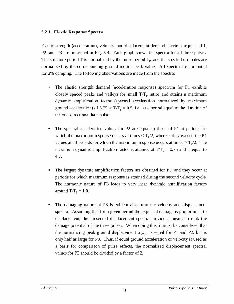
Chapter 5 Pulse-Type Seismic Input 71
5.2.1. Elastic Response Spectra Elastic strength (acceleration), velocity, and displacement demand spectra for pulses P1, P2, and P3 are presented in Fig. 5.4. Each graph shows the spectra for all three pulses. The structure period T is normalized by the pulse period Tp, and the spectral ordinates are normalized by the corresponding ground motion peak value. All spectra are computed for 2% damping. The following observations are made from the spectra:
• = The elastic strength demand (acceleration response) spectrum for P1 exhibits closely spaced peaks and valleys for small T/Tp ratios and attains a maximum dynamic amplification factor (spectral acceleration normalized by maximum ground acceleration) of 3.75 at T/Tp = 0.5, i.e., at a period equal to the duration of the one-directional half-pulse.
• = The spectral acceleration values for P2 are equal to those of P1 at periods for
which the maximum response occurs at times ≤ Tp/2, whereas they exceed the P1 values at all periods for which the maximum response occurs at times > Tp/2. The maximum dynamic amplification factor is attained at T/Tp = 0.75 and is equal to 4.7.
• = The largest dynamic amplification factors are obtained for P3, and they occur at
periods for which maximum response is attained during the second velocity cycle. The harmonic nature of P3 leads to very large dynamic amplification factors around T/Tp = 1.0.
• = The damaging nature of P3 is evident also from the velocity and displacement
spectra. Assuming that for a given period the expected damage is proportional to displacement, the presented displacement spectra provide a means to rank the damage potential of the three pulses. When doing this, it must be considered that the normalizing peak ground displacement ug,max is equal for P1 and P2, but is only half as large for P3. Thus, if equal ground acceleration or velocity is used as a basis for comparison of pulse effects, the normalized displacement spectral values for P3 should be divided by a factor of 2.
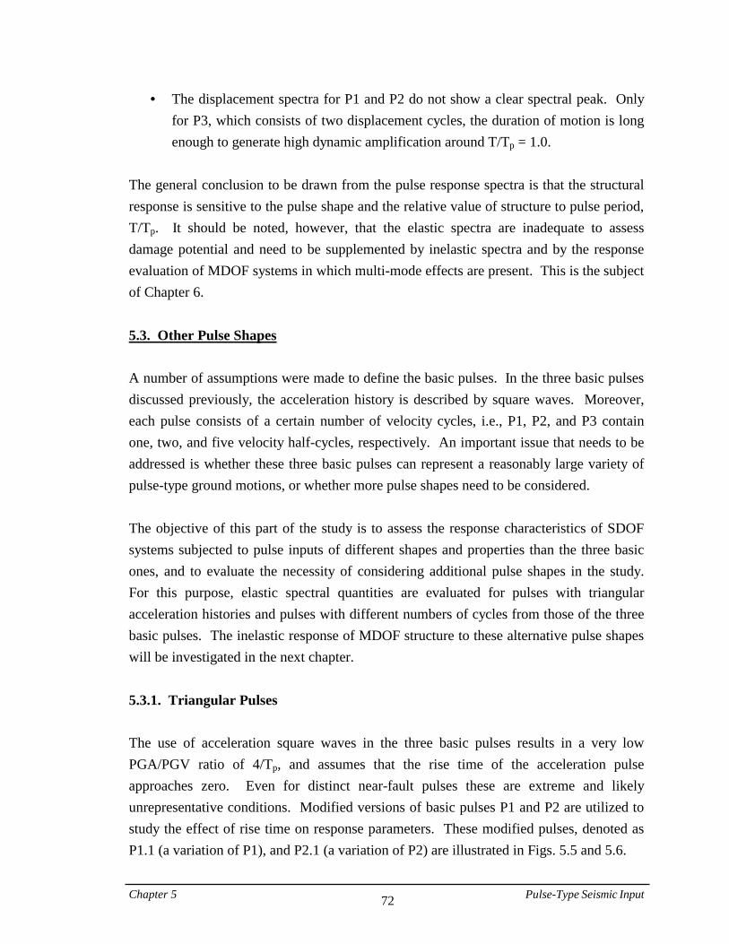
Chapter 5 Pulse-Type Seismic Input 72
• = The displacement spectra for P1 and P2 do not show a clear spectral peak. Only for P3, which consists of two displacement cycles, the duration of motion is long enough to generate high dynamic amplification around T/Tp = 1.0.
The general conclusion to be drawn from the pulse response spectra is that the structural response is sensitive to the pulse shape and the relative value of structure to pulse period, T/Tp. It should be noted, however, that the elastic spectra are inadequate to assess damage potential and need to be supplemented by inelastic spectra and by the response evaluation of MDOF systems in which multi-mode effects are present. This is the subject of Chapter 6. 5.3. Other Pulse Shapes A number of assumptions were made to define the basic pulses. In the three basic pulses discussed previously, the acceleration history is described by square waves. Moreover, each pulse consists of a certain number of velocity cycles, i.e., P1, P2, and P3 contain one, two, and five velocity half-cycles, respectively. An important issue that needs to be addressed is whether these three basic pulses can represent a reasonably large variety of pulse-type ground motions, or whether more pulse shapes need to be considered. The objective of this part of the study is to assess the response characteristics of SDOF systems subjected to pulse inputs of different shapes and properties than the three basic ones, and to evaluate the necessity of considering additional pulse shapes in the study. For this purpose, elastic spectral quantities are evaluated for pulses with triangular acceleration histories and pulses with different numbers of cycles from those of the three basic pulses. The inelastic response of MDOF structure to these alternative pulse shapes will be investigated in the next chapter. 5.3.1. Triangular Pulses The use of acceleration square waves in the three basic pulses results in a very low PGA/PGV ratio of 4/Tp, and assumes that the rise time of the acceleration pulse approaches zero. Even for distinct near-fault pulses these are extreme and likely unrepresentative conditions. Modified versions of basic pulses P1 and P2 are utilized to study the effect of rise time on response parameters. These modified pulses, denoted as P1.1 (a variation of P1), and P2.1 (a variation of P2) are illustrated in Figs. 5.5 and 5.6.
Chapter 5 Pulse-Type Seismic Input 73
If the peak parameters (PGA, PGV, and PGD) of the pulse variations are normalized by the corresponding parameter of the basic pulses and the PGV ratio is set equal to 1.0, it is observed that no difference exists in the peak ground displacements, but that in both cases the PGA of the modified pulse is twice that of the basic pulse. Thus, the PGA/PGV ratio is 8/Tp, which is in the range of values observed in “ordinary” records from past earthquakes (Lawson, 1996) – if Tp is on the order of 1 sec. or shorter. Elastic Response Spectra: The effect of these pulse modifications on spectral response is documented in Figs. 5.7 and 5.8. The spectra of the modified pulses are shown in heavy lines and the spectra of the corresponding basic pulses are shown in light lines. Each pulse response spectrum is normalized by the peak value of the corresponding pulse input. These peak values are shown in Figs. 5.1, 5.2, 5.5, and 5.6. Since the PGV and PGD values of both modified pulses are identical to those of the basic pulses, and the normalized velocity and displacement spectra do not differ by much, it is concluded that the pulse modifications have a relatively small effect on spectral velocity and displacement responses. This appears to be not so for the spectral acceleration responses. The normalized spectral accelerations (dynamic amplification factors) for the modified pulses are much smaller than those for the basic pulses. However, the PGA values of the modified pulses are twice as large as those of the basic pulses. Once this is considered, it is observed that the difference in spectral accelerations between the modified and basic pulses is not drastic at most periods. It is concluded that the spectral response of the modified pulses with triangular acceleration histories can be adequately represented by their corresponding basic pulses. The effect of these triangular pulses on the response of MDOF structures is studied in the next chapter. 5.3.2. Pulse Histories with Different Duration The period of the basic pulses (Tp) is defined as the time needed to complete a full velocity cycle. Based on this definition, the duration of basic pulse histories P1, P2, and P3 is 0.5, 1.0, and 2.5 times the pulse period, respectively. There are pulse histories with different duration whose response properties may need to be evaluated. Two additional

Chapter 5 Pulse-Type Seismic Input 74
pulses, P4 and P5, are introduced and studied here for this purpose. The acceleration time histories for P4 and P5 are described by the square waves shown in Figs. 5.9 and 5.10. The duration of these two pulse histories is 1.5Tp for P4 and 2.0Tp for P5. It should be noted that the duration of these new pulses is between those of P2 and P3. Thus, it is useful to compare the response characteristics of P4 and P5 with those of basic pulses P2 and P3. Elastic Response Spectra: The elastic strength (acceleration), velocity, and displacement demand spectra of all five pulses P1 to P5 are compared in Fig. 5.11. The spectral ordinates are normalized by the corresponding time history peak values. The following observations can be made from the spectra:
• = The spectra of P4 and P5 exhibit patterns similar to those of P3 but with smaller peak values.
• = The normalized spectral displacements for P4 and P5 are bounded by the
corresponding values for P2 and P3. However, this does not hold true at all periods for the normalized spectral acceleration and velocity values.
Since the spectral responses for P4 and P5 are not always close to those for basic pulses P1, P2, and P3 in the full range of T/Tp, more investigation is necessary to quantify the MDOF response characteristics of pulses P4 and P5. The inelastic demands of MDOF structures subjected to pulse shapes P4 and P5 are evaluated in the next chapter.
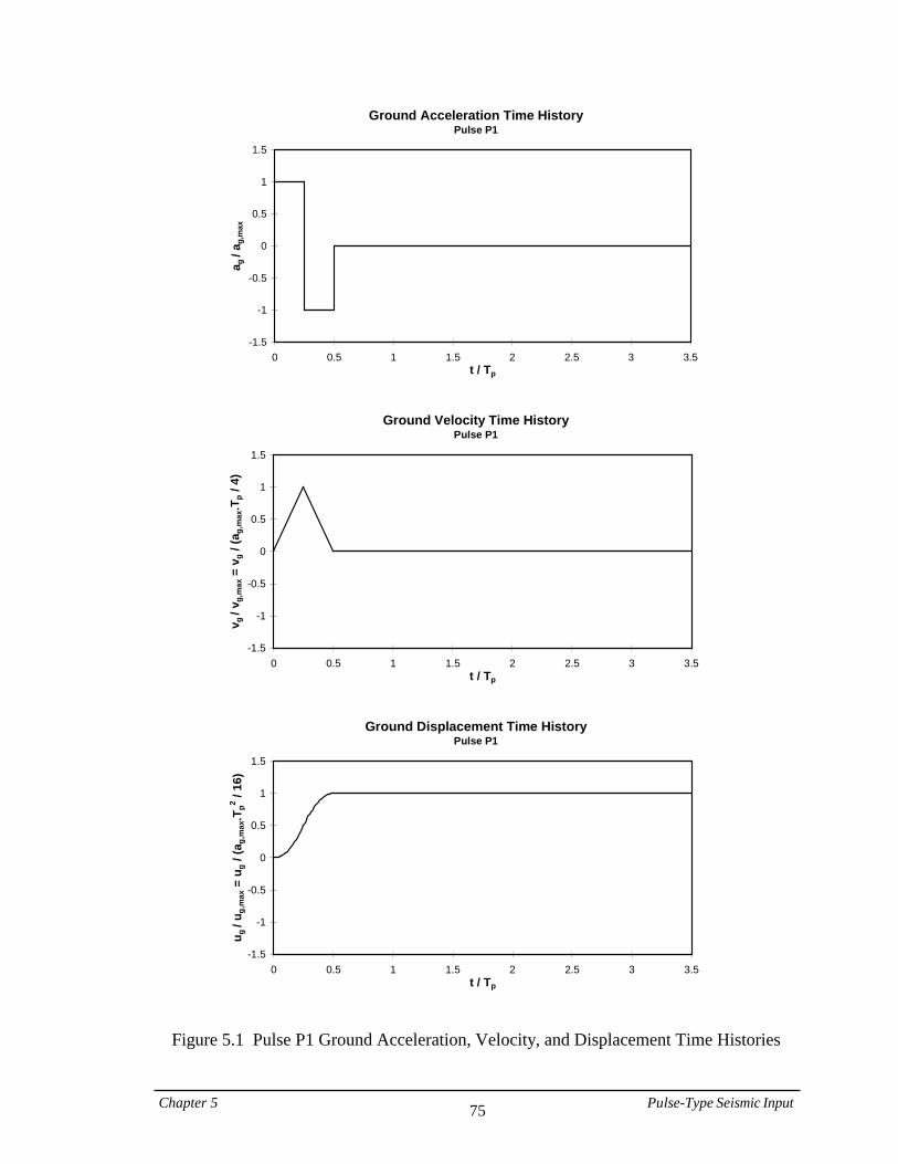
Chapter 5 Pulse-Type Seismic Input 75
Ground Acceleration Time HistoryPulse P1
-1.5
-1
-0.5
0
0.5
1
1.5
0 0.5 1 1.5 2 2.5 3 3.5t / Tp
a g /
a g,m
ax
Ground Velocity Time HistoryPulse P1
-1.5
-1
-0.5
0
0.5
1
1.5
0 0.5 1 1.5 2 2.5 3 3.5t / Tp
v g /
v g,m
ax =
vg /
(ag,
max
.Tp /
4)
Ground Displacement Time HistoryPulse P1
-1.5
-1
-0.5
0
0.5
1
1.5
0 0.5 1 1.5 2 2.5 3 3.5t / Tp
u g /
u g,m
ax =
ug /
(ag,
max
.Tp2 /
16)
Figure 5.1 Pulse P1 Ground Acceleration, Velocity, and Displacement Time Histories
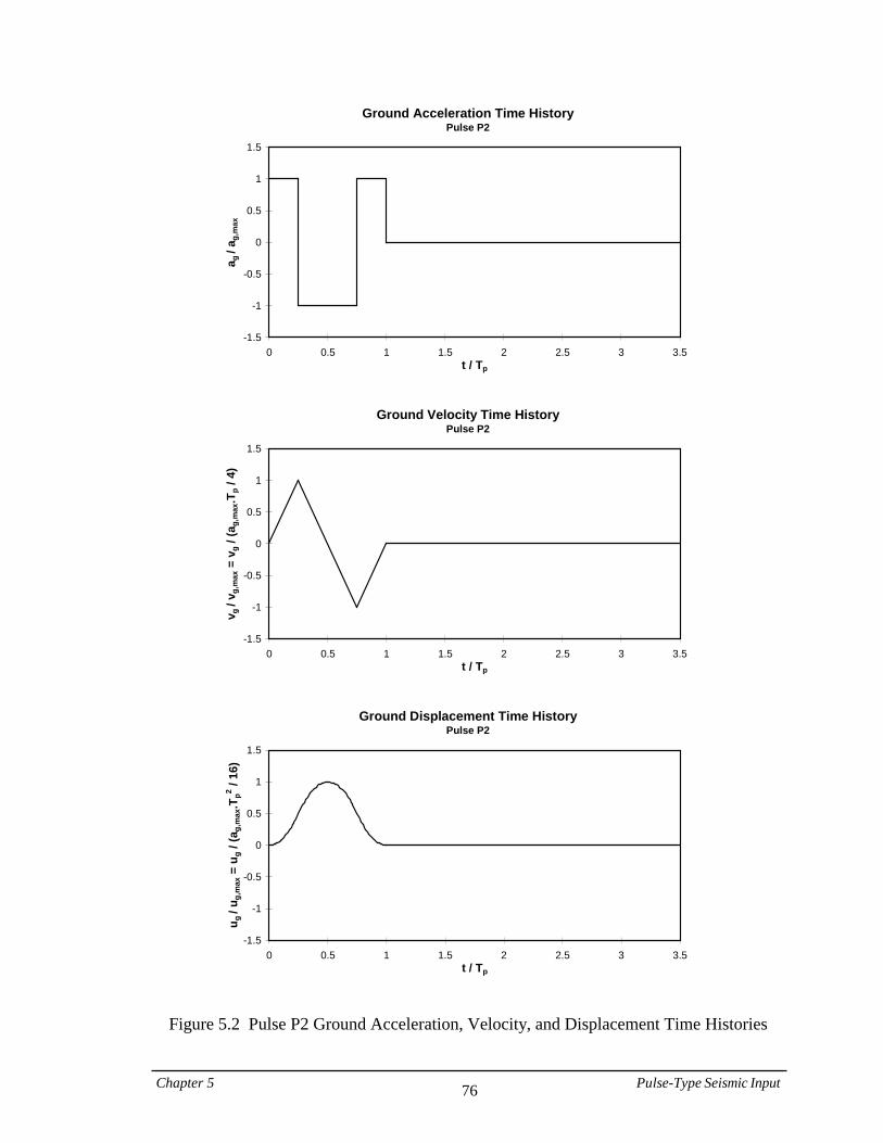
Chapter 5 Pulse-Type Seismic Input 76
Ground Acceleration Time HistoryPulse P2
-1.5
-1
-0.5
0
0.5
1
1.5
0 0.5 1 1.5 2 2.5 3 3.5t / Tp
a g /
a g,m
ax
Ground Velocity Time HistoryPulse P2
-1.5
-1
-0.5
0
0.5
1
1.5
0 0.5 1 1.5 2 2.5 3 3.5t / Tp
v g /
v g,m
ax =
vg /
(ag,
max
.Tp /
4)
Ground Displacement Time HistoryPulse P2
-1.5
-1
-0.5
0
0.5
1
1.5
0 0.5 1 1.5 2 2.5 3 3.5t / Tp
u g /
u g,m
ax =
ug /
(ag,
max
.Tp2 /
16)
Figure 5.2 Pulse P2 Ground Acceleration, Velocity, and Displacement Time Histories

Chapter 5 Pulse-Type Seismic Input 77
Ground Acceleration Time HistoryPulse P3
-1.5
-1
-0.5
0
0.5
1
1.5
0 0.5 1 1.5 2 2.5 3 3.5t / Tp
a g /
a g,m
ax
Ground Velocity Time HistoryPulse P3
-1.5
-1
-0.5
0
0.5
1
1.5
0 0.5 1 1.5 2 2.5 3 3.5t / Tp
v g /
v g,m
ax =
vg /
(ag,
max
.Tp /
4)
Ground Displacement Time HistoryPulse P3
-1.5
-1
-0.5
0
0.5
1
1.5
0 0.5 1 1.5 2 2.5 3 3.5t / Tp
u g /
u g,m
ax =
ug /
(ag,
max
.Tp2 /
32)
Figure 5.3 Pulse P3 Ground Acceleration, Velocity, and Displacement Time Histories
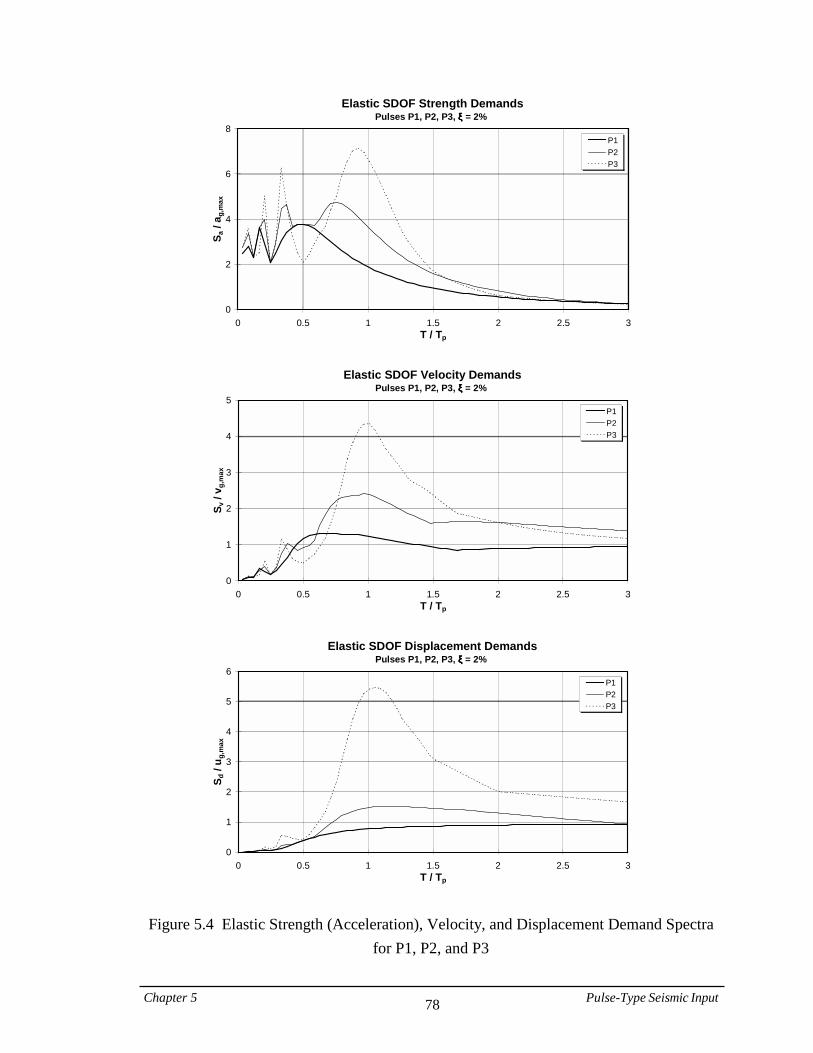
Chapter 5 Pulse-Type Seismic Input 78
Elastic SDOF Strength DemandsPulses P1, P2, P3, ξξξξ = 2%
0
2
4
6
8
0 0.5 1 1.5 2 2.5 3T / Tp
S a /
a g,m
ax
P1P2P3
Elastic SDOF Velocity DemandsPulses P1, P2, P3, ξξξξ = 2%
0
1
2
3
4
5
0 0.5 1 1.5 2 2.5 3T / Tp
S v /
v g,m
ax
P1P2P3
Elastic SDOF Displacement DemandsPulses P1, P2, P3, ξξξξ = 2%
0
1
2
3
4
5
6
0 0.5 1 1.5 2 2.5 3T / Tp
S d /
u g,m
ax
P1P2P3
Figure 5.4 Elastic Strength (Acceleration), Velocity, and Displacement Demand Spectra for P1, P2, and P3
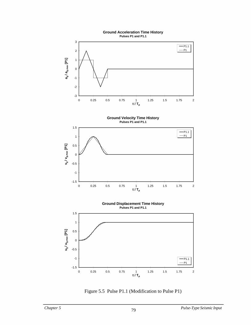
Chapter 5 Pulse-Type Seismic Input 79
Ground Acceleration Time HistoryPulses P1 and P1.1
-3
-2
-1
0
1
2
3
0 0.25 0.5 0.75 1 1.25 1.5 1.75 2t / Tp
a g /
a g,m
ax [P
1]
P1.1P1
Ground Velocity Time HistoryPulses P1 and P1.1
-1.5
-1
-0.5
0
0.5
1
1.5
0 0.25 0.5 0.75 1 1.25 1.5 1.75 2t / Tp
v g /
v g,m
ax [P
1]
P1.1P1
Ground Displacement Time HistoryPulses P1 and P1.1
-1.5
-1
-0.5
0
0.5
1
1.5
0 0.25 0.5 0.75 1 1.25 1.5 1.75 2t / Tp
u g /
u g,m
ax [P
1]
P1.1P1
Figure 5.5 Pulse P1.1 (Modification to Pulse P1)
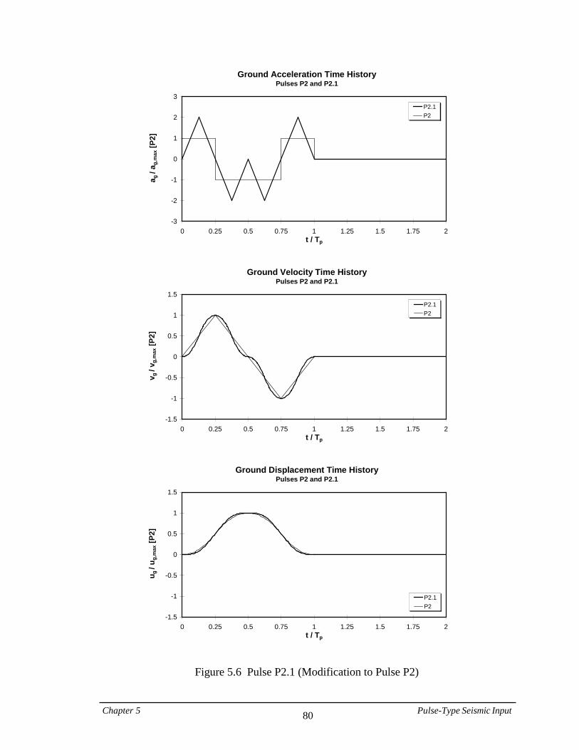
Chapter 5 Pulse-Type Seismic Input 80
Ground Acceleration Time HistoryPulses P2 and P2.1
-3
-2
-1
0
1
2
3
0 0.25 0.5 0.75 1 1.25 1.5 1.75 2t / Tp
a g /
a g,m
ax [P
2]
P2.1P2
Ground Velocity Time HistoryPulses P2 and P2.1
-1.5
-1
-0.5
0
0.5
1
1.5
0 0.25 0.5 0.75 1 1.25 1.5 1.75 2t / Tp
v g /
v g,m
ax [P
2]
P2.1P2
Ground Displacement Time HistoryPulses P2 and P2.1
-1.5
-1
-0.5
0
0.5
1
1.5
0 0.25 0.5 0.75 1 1.25 1.5 1.75 2t / Tp
u g /
u g,m
ax [P
2]
P2.1P2
Figure 5.6 Pulse P2.1 (Modification to Pulse P2)
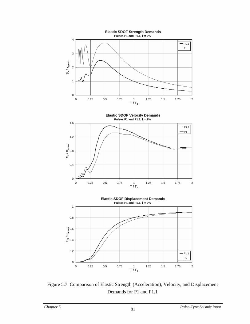
Chapter 5 Pulse-Type Seismic Input 81
Elastic SDOF Strength DemandsPulses P1 and P1.1, ξξξξ = 2%
0
1
2
3
4
0 0.25 0.5 0.75 1 1.25 1.5 1.75 2T / Tp
S a /
a g,m
ax
P1.1
P1
Elastic SDOF Velocity DemandsPulses P1 and P1.1, ξξξξ = 2%
0
0.4
0.8
1.2
1.6
0 0.25 0.5 0.75 1 1.25 1.5 1.75 2T / Tp
S v /
v g,m
ax
P1.1
P1
Elastic SDOF Displacement DemandsPulses P1 and P1.1, ξξξξ = 2%
0
0.2
0.4
0.6
0.8
1
0 0.25 0.5 0.75 1 1.25 1.5 1.75 2T / Tp
S d /
u g,m
ax
P1.1
P1
Figure 5.7 Comparison of Elastic Strength (Acceleration), Velocity, and Displacement Demands for P1 and P1.1
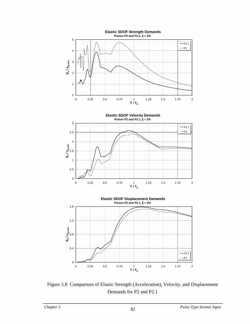
Chapter 5 Pulse-Type Seismic Input 82
Elastic SDOF Strength DemandsPulses P2 and P2.1, ξξξξ = 2%
0
1
2
3
4
5
0 0.25 0.5 0.75 1 1.25 1.5 1.75 2T / Tp
S a /
a g,m
ax
P2.1
P2
Elastic SDOF Velocity DemandsPulses P2 and P2.1, ξξξξ = 2%
0
0.5
1
1.5
2
2.5
3
0 0.25 0.5 0.75 1 1.25 1.5 1.75 2T / Tp
S v /
v g,m
ax
P2.1
P2
Elastic SDOF Displacement DemandsPulses P2 and P2.1, ξξξξ = 2%
0
0.4
0.8
1.2
1.6
0 0.25 0.5 0.75 1 1.25 1.5 1.75 2T / Tp
S d /
u g,m
ax
P2.1
P2
Figure 5.8 Comparison of Elastic Strength (Acceleration), Velocity, and Displacement Demands for P2 and P2.1

Chapter 5 Pulse-Type Seismic Input 83
Ground Acceleration Time HistoryPulse P4
-1.5
-1
-0.5
0
0.5
1
1.5
0 0.5 1 1.5 2 2.5 3 3.5t / Tp
a g /
a g,m
ax
Ground Velocity Time History
Pulse P4
-1.5
-1
-0.5
0
0.5
1
1.5
0 0.5 1 1.5 2 2.5 3 3.5t / Tp
v g /
v g,m
ax =
vg /
(ag,
max
.Tp /
4)
Ground Displacement Time History
Pulse P4
-1.5
-1
-0.5
0
0.5
1
1.5
0 0.5 1 1.5 2 2.5 3 3.5t / Tp
u g /
u g,m
ax =
ug /
(ag,
max
.Tp2 /
32)
Figure 5.9 Pulse P4 Ground Acceleration, Velocity, and Displacement Time Histories
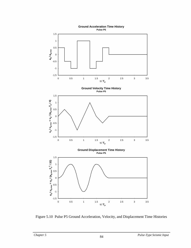
Chapter 5 Pulse-Type Seismic Input 84
Ground Acceleration Time HistoryPulse P5
-1.5
-1
-0.5
0
0.5
1
1.5
0 0.5 1 1.5 2 2.5 3 3.5t / Tp
a g /
a g,m
ax
Ground Velocity Time History
Pulse P5
-1.5
-1
-0.5
0
0.5
1
1.5
0 0.5 1 1.5 2 2.5 3 3.5t / Tp
v g /
v g,m
ax =
vg /
(ag,
max
.Tp /
4)
Ground Displacement Time History
Pulse P5
-1.5
-1
-0.5
0
0.5
1
1.5
0 0.5 1 1.5 2 2.5 3 3.5t / Tp
u g /
u g,m
ax =
ug /
(ag,
max
.Tp2 /
32)
Figure 5.10 Pulse P5 Ground Acceleration, Velocity, and Displacement Time Histories
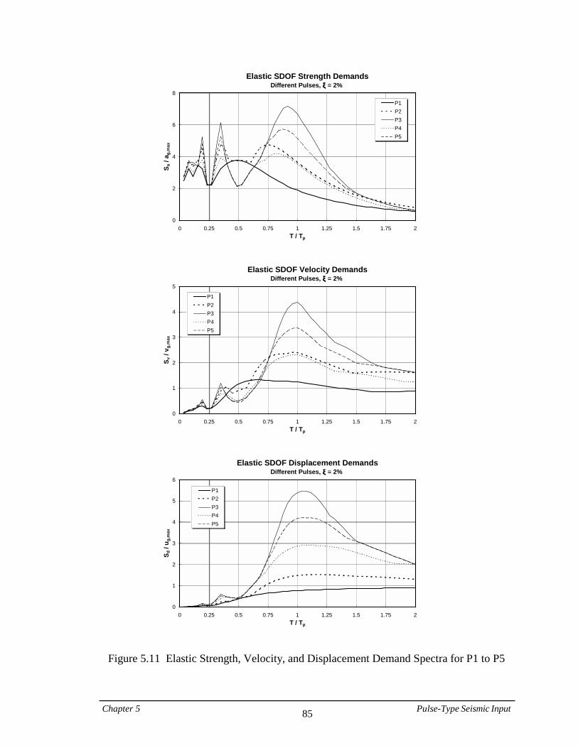
Chapter 5 Pulse-Type Seismic Input 85
Elastic SDOF Strength DemandsDifferent Pulses, ξξξξ = 2%
0
2
4
6
8
0 0.25 0.5 0.75 1 1.25 1.5 1.75 2T / Tp
S a /
a g,m
ax
P1P2P3P4P5
Elastic SDOF Velocity DemandsDifferent Pulses, ξξξξ = 2%
0
1
2
3
4
5
0 0.25 0.5 0.75 1 1.25 1.5 1.75 2T / Tp
S v /
v g,m
ax
P1P2P3P4P5
Elastic SDOF Displacement DemandsDifferent Pulses, ξξξξ = 2%
0
1
2
3
4
5
6
0 0.25 0.5 0.75 1 1.25 1.5 1.75 2T / Tp
S d /
u g,m
ax
P1P2P3P4P5
Figure 5.11 Elastic Strength, Velocity, and Displacement Demand Spectra for P1 to P5
Chapter 6 Response of Structures to Pulse-Type … 86
CHAPTER 6
RESPONSE OF STRUCTURES TO PULSE-TYPE SEISMIC INPUT
This Chapter is devoted to evaluating the response of elastic and inelastic structures to pulse-type seismic input, and achieving a fundamental understanding of response characteristics that can be utilized later (in Chapter 7) in the representation of near-fault ground motions by equivalent pulses. The SDOF and MDOF structures introduced in Chapter 3 and the pulse-type ground motions defined in Chapter 5 are employed in the pulse response evaluations. First, the elastic response of MDOF frame structures to the pulse-type input motions is investigated. Elastic base shear demands and the distribution of story shear demands over the height of the structure are evaluated. The goal is to identify the response characteristics and patterns that near-fault ground motions and simple pulses have in common. Then, comprehensive response studies are carried out on inelastic SDOF systems and MDOF frame structures subjected to the basic pulses. Story ductility demands are utilized to evaluate the performance of inelastic MDOF systems. Inelastic roof displacement and story drift demands are also quantified. Generic 3- and 9-story frame structures are introduced and utilized to assess the sensitivity of the response of MDOF structures to the number of stories. Finally, a pilot study is carried out whose objective is to quantify the response to pulse-type ground motions of frame structures in which plastic hinges can develop only at the end of columns. 6.1. Elastic Response of MDOF Structures to Pulse-Type Input The basic assumptions and procedures employed in the design of the generic 20-story structure were introduced in Section 3.2. In the pulse study, MDOF dynamic analyses
Chapter 6 Response of Structures to Pulse-Type … 87
are performed primarily for T/Tp = 0.375, 0.50, 0.75, 1.0, 1.5, 2.0, and 3.0, where T is the structure fundamental period and Tp represents the pulse period defined in Section 5.2. 6.1.1. Deflected Shapes of Structure Snapshots of the deflected shapes of the generic MDOF structures subjected to the basic pulses at intervals of Tp/4 are shown in Figs. 6.1 to 6.4. The deflected shapes serve to illustrate the effect of pulse loading on the structural response at specific time steps. Figure 6.1 corresponds to a structure with T = 0.5Tp subjected to P1. It can be seen that for this short period structure the deflected shape is similar to a first mode shape, signifying that higher-mode effects are insignificant and the dynamic behavior is controlled mostly by the first mode. The maximum roof displacement value of 0.55ug,max occurs at t = Tp/2, i.e., the beginning of the free vibration phase. Figures 6.2 to 6.4 illustrate deflected shapes for a structure with T = 2Tp subjected to all three basic pulses. The following observations are made:
• = For all pulses the deflected shape, which is far from a straight line, clearly shows higher mode contributions and the effect of a transient wave traveling up the structure.
• = The deflected shapes for P1 and P2 are identical until Tp/2, at which time the
structure subjected to P1 enters the free vibration phase. The roof displacement at this instance is very close to the ground displacement, which is at its maximum. Under P1 the structure reaches its maximum roof displacement of 1.3ug,max in the free vibration phase at t = Tp because enough energy is stored in the structure during the half-pulse input to increase the roof displacement by 30% during the first free vibration reversal.
• = The structure subjected to P2 also reaches its maximum roof displacement at t =
Tp, but because of the reversal of ground displacement, the maximum roof displacement of 2.3ug,max is significantly larger than the corresponding value for P1.
• = The largest roof displacement of 3.9ug,max is observed for the structure subjected
to P3. It occurs at t = 1.5Tp, the time of the peak of the second ground
Chapter 6 Response of Structures to Pulse-Type … 88
displacement cycle. Thus, the harmonic nature of P3 has a larger effect on the roof displacement compared to P2, which has only one displacement pulse.
6.1.2. Maximum Elastic Base Shear Force Today's design procedures are based on specification of a base shear and a distribution of story shear forces over the height of the structure. The base shear is usually evaluated from the first mode spectral strength demand, with modifications applied to account for higher-mode effects. Thus, an evaluation of base shear demands and their relation to the first mode spectral values contributes to the understanding of pulse response. Elastic base shear strength demands for the generic structures with various periods subjected to all three basic pulses are presented in Fig. 6.5. The base shear demands are normalized by m.ag,max, so that the results are comparable with the SDOF strength demand spectra presented in Fig. 5.4. This comparison is made in Fig. 6.6, which illustrates ratios of MDOF base shear to SDOF strength demands at the first mode period. The following observations are made:
• = The ratios are sensitive to the pulse type and T/Tp, and may easily exceed 1.0 for larger T/Tp ratios, signifying large higher-mode effects.
• = The variation of the elastic base shear demands for each pulse typically follows
the same pattern as its corresponding SDOF strength demand spectrum. The base shear demand for P1 and P2 is highest at relatively small T/Tp ratios.
• = The maximum base shear demand for P3 occurs at T/Tp = 1.0, which can be
attributed to the harmonic nature of this pulse. A similar observation has been made by Rahnama and Krawinkler (1993) in their study on response to soft soil motions, which have characteristics similar to those of P3.
Study on Continuous Shear Building with Uniform Properties: Hall et al. (1995) studied the effects of pulses P1 and P2 on an undamped continuous shear building with uniform shear stiffness over the height, based on elastic wave propagation theory. They presented their results for specific T/Tp values in terms of shear strain at the base of the building. In this study their approach is generalized to
Chapter 6 Response of Structures to Pulse-Type … 89
include also pulse P3, and the maximum base shear is calculated for the range of T/Tp from 0 to 3.0. The results for base shear demands obtained from a closed form solution are presented in Fig. 6.7, along with the time history of the base shear force for P2 and T/Tp = 0.75 in Fig. 6.8. A relatively consistent correlation is observed between the demands for the continuous shear building and those for the generic structure. The elastic base shear demands for the continuous shear building are typically larger than the corresponding demands for the generic 20-story structure. In part, this can be attributed to the fact that no damping is considered in the shear building model. However, it is believed that the effect of damping is not large (see Section 6.2.2), and that the difference in the elastic base shear demands has to do with the fact that unlike the generic structure, the continuous shear building has constant stiffness over the height. 6.1.3. Distribution of Elastic Story Shear Over Height Figure 6.9 compares the SRSS story shear distribution used in the design of the structures (denoted as “Design”), with elastic story shear distributions obtained from (a) time history analyses and (b) SRSS modal combinations using the corresponding pulse spectrum for pulses P1 to P3 and various T/Tp ratios. The following observations are made:
• = For structures with T/Tp ≤ 1.0, the dynamic shear force distributions are relatively smooth, but for structures with T/Tp > 1.0 the distributions show a clear effect of a wave traveling up the structure. This effect is evident for P1, more evident for P2, and most evident for P3. In the last case the maximum elastic story shear demand for T/Tp = 2.0 occurs about 2/3rd up the height of the structure rather than at the base. Thus, for long period structures (T/Tp > 1.0) designed according to a standard SRSS story shear strength distribution, early yielding has to be expected in the upper stories.
• = For MDOF structures with T/Tp > 1.0, the SRSS modal combination is not a good
substitute for the dynamic time history analysis. This observation provides an indication that spectral analysis may not capture all important response characteristics of pulse-type ground motions, once higher-mode effects become important.
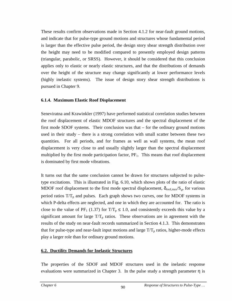
Chapter 6 Response of Structures to Pulse-Type … 90
These results confirm observations made in Section 4.1.2 for near-fault ground motions, and indicate that for pulse-type ground motions and structures whose fundamental period is larger than the effective pulse period, the design story shear strength distribution over the height may need to be modified compared to presently employed design patterns (triangular, parabolic, or SRSS). However, it should be considered that this conclusion applies only to elastic or nearly elastic structures, and that the distributions of demands over the height of the structure may change significantly at lower performance levels (highly inelastic systems). The issue of design story shear strength distributions is pursued in Chapter 9. 6.1.4. Maximum Elastic Roof Displacement Seneviratna and Krawinkler (1997) have performed statistical correlation studies between the roof displacement of elastic MDOF structures and the spectral displacement of the first mode SDOF systems. Their conclusion was that – for the ordinary ground motions used in their study – there is a strong correlation with small scatter between these two quantities. For all periods, and for frames as well as wall systems, the mean roof displacement is very close to and usually slightly larger than the spectral displacement multiplied by the first mode participation factor, PF1. This means that roof displacement is dominated by first mode vibrations. It turns out that the same conclusion cannot be drawn for structures subjected to pulse-type excitations. This is illustrated in Fig. 6.10, which shows plots of the ratio of elastic MDOF roof displacement to the first mode spectral displacement, δroof,max/Sd, for various
period ratios T/Tp and pulses. Each graph shows two curves, one for MDOF systems in which P-delta effects are neglected, and one in which they are accounted for. The ratio is close to the value of PF1 (1.37) for T/Tp ≤ 1.0, and consistently exceeds this value by a significant amount for large T/Tp ratios. These observations are in agreement with the results of the study on near-fault records summarized in Section 4.1.3. This demonstrates that for pulse-type and near-fault input motions and large T/Tp ratios, higher-mode effects play a larger role than for ordinary ground motions. 6.2. Ductility Demands for Inelastic Structures The properties of the SDOF and MDOF structures used in the inelastic response evaluations were summarized in Chapter 3. In the pulse study a strength parameter η is
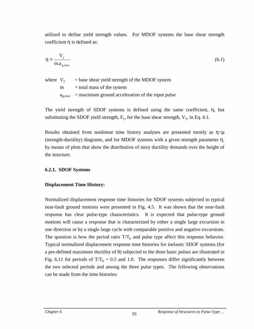
Chapter 6 Response of Structures to Pulse-Type … 91
utilized to define yield strength values. For MDOF systems the base shear strength coefficient η is defined as:
max,g
y
a.mV
=η (6.1)
where Vy = base shear yield strength of the MDOF system m = total mass of the system ag,max = maximum ground acceleration of the input pulse The yield strength of SDOF systems is defined using the same coefficient, η, but substituting the SDOF yield strength, Fy, for the base shear strength, Vy, in Eq. 6.1. Results obtained from nonlinear time history analyses are presented mostly as η−µ (strength-ductility) diagrams, and for MDOF systems with a given strength parameter η, by means of plots that show the distribution of story ductility demands over the height of the structure. 6.2.1. SDOF Systems Displacement Time History: Normalized displacement response time histories for SDOF systems subjected to typical near-fault ground motions were presented in Fig. 4.5. It was shown that the near-fault response has clear pulse-type characteristics. It is expected that pulse-type ground motions will cause a response that is characterized by either a single large excursion in one direction or by a single large cycle with comparable positive and negative excursions. The question is how the period ratio T/Tp and pulse type affect this response behavior. Typical normalized displacement response time histories for inelastic SDOF systems (for a pre-defined maximum ductility of 8) subjected to the three basic pulses are illustrated in Fig. 6.11 for periods of T/Tp = 0.5 and 1.0. The responses differ significantly between the two selected periods and among the three pulse types. The following observations can be made from the time histories:
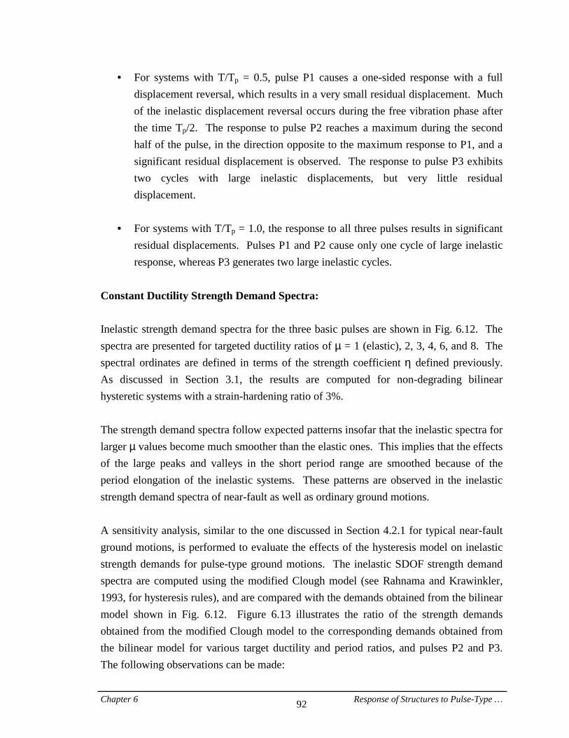
Chapter 6 Response of Structures to Pulse-Type … 92
• = For systems with T/Tp = 0.5, pulse P1 causes a one-sided response with a full displacement reversal, which results in a very small residual displacement. Much of the inelastic displacement reversal occurs during the free vibration phase after the time Tp/2. The response to pulse P2 reaches a maximum during the second half of the pulse, in the direction opposite to the maximum response to P1, and a significant residual displacement is observed. The response to pulse P3 exhibits two cycles with large inelastic displacements, but very little residual displacement.
• = For systems with T/Tp = 1.0, the response to all three pulses results in significant
residual displacements. Pulses P1 and P2 cause only one cycle of large inelastic response, whereas P3 generates two large inelastic cycles.
Constant Ductility Strength Demand Spectra: Inelastic strength demand spectra for the three basic pulses are shown in Fig. 6.12. The spectra are presented for targeted ductility ratios of µ = 1 (elastic), 2, 3, 4, 6, and 8. The spectral ordinates are defined in terms of the strength coefficient η defined previously. As discussed in Section 3.1, the results are computed for non-degrading bilinear hysteretic systems with a strain-hardening ratio of 3%. The strength demand spectra follow expected patterns insofar that the inelastic spectra for larger µ values become much smoother than the elastic ones. This implies that the effects of the large peaks and valleys in the short period range are smoothed because of the period elongation of the inelastic systems. These patterns are observed in the inelastic strength demand spectra of near-fault as well as ordinary ground motions. A sensitivity analysis, similar to the one discussed in Section 4.2.1 for typical near-fault ground motions, is performed to evaluate the effects of the hysteresis model on inelastic strength demands for pulse-type ground motions. The inelastic SDOF strength demand spectra are computed using the modified Clough model (see Rahnama and Krawinkler, 1993, for hysteresis rules), and are compared with the demands obtained from the bilinear model shown in Fig. 6.12. Figure 6.13 illustrates the ratio of the strength demands obtained from the modified Clough model to the corresponding demands obtained from the bilinear model for various target ductility and period ratios, and pulses P2 and P3. The following observations can be made:
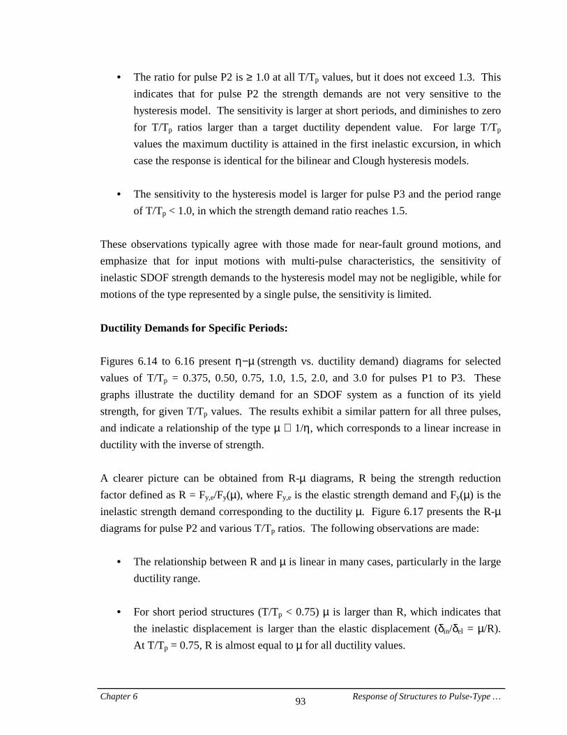
Chapter 6 Response of Structures to Pulse-Type … 93
• = The ratio for pulse P2 is ≥ 1.0 at all T/Tp values, but it does not exceed 1.3. This indicates that for pulse P2 the strength demands are not very sensitive to the hysteresis model. The sensitivity is larger at short periods, and diminishes to zero for T/Tp ratios larger than a target ductility dependent value. For large T/Tp values the maximum ductility is attained in the first inelastic excursion, in which case the response is identical for the bilinear and Clough hysteresis models.
• = The sensitivity to the hysteresis model is larger for pulse P3 and the period range
of T/Tp < 1.0, in which the strength demand ratio reaches 1.5. These observations typically agree with those made for near-fault ground motions, and emphasize that for input motions with multi-pulse characteristics, the sensitivity of inelastic SDOF strength demands to the hysteresis model may not be negligible, while for motions of the type represented by a single pulse, the sensitivity is limited. Ductility Demands for Specific Periods: Figures 6.14 to 6.16 present η−µ=(strength vs. ductility demand) diagrams for selected values of T/Tp = 0.375, 0.50, 0.75, 1.0, 1.5, 2.0, and 3.0 for pulses P1 to P3. These graphs illustrate the ductility demand for an SDOF system as a function of its yield strength, for given T/Tp values. The results exhibit a similar pattern for all three pulses, and indicate a relationship of the type µ ∝ 1/η, which corresponds to a linear increase in ductility with the inverse of strength. A clearer picture can be obtained from R-µ diagrams, R being the strength reduction factor defined as R = Fy,e/Fy(µ), where Fy,e is the elastic strength demand and Fy(µ) is the inelastic strength demand corresponding to the ductility µ. Figure 6.17 presents the R-µ diagrams for pulse P2 and various T/Tp ratios. The following observations are made:
• = The relationship between R and µ is linear in many cases, particularly in the large ductility range.
• = For short period structures (T/Tp < 0.75) µ is larger than R, which indicates that
the inelastic displacement is larger than the elastic displacement (δin/δel = µ/R). At T/Tp = 0.75, R is almost equal to µ for all ductility values.
Chapter 6 Response of Structures to Pulse-Type … 94
• = For structures with 0.75 < T/Tp < 3.0, R becomes larger than µ, indicating that the elastic displacement is larger than the inelastic displacement. For very long period structures (T/Tp = 3.0), R approaches µ for all ductility values. The reason is that at very long periods both elastic and inelastic displacements approach the maximum ground displacements regardless of the structure strength.
The patterns observed previously for R-µ-T relationships can be seen also from δin/δel ratios (see Section 6.3.1). A one-to-one comparison of the ductility demands for the three basic pulses is illustrated in Fig. 6.18, which shows η−µ and R−µ graphs for T/Tp = 0.5 and 2.0. The following observations are made:
• = For given strength (η value) the results show significant pulse-type dependence at T/Tp = 0.5, whereas the demands at T/Tp = 2.0 are less dependent on pulse type. A general comparison of the results for different pulses indicates that for a given strength level and T/Tp ratio, P2 always causes a larger or at least equal ductility demand compared to P1. The reason is that pulses P1 and P2 have identical ground time histories up to t = Tp/2, and P1 comes to rest thereafter.
• = At T/Tp = 0.5 and for a given ductility ratio, R is largest for P1 and smallest for
P3. At T/Tp = 2.0 pulse P2 corresponds to the largest R value regardless of µ, but the pulse type corresponding to the smallest R value depends on the ductility ratio. The pulse-type dependence of the R-µ relationship is significant for short period structures, and becomes less so for long period structures.
6.2.2. MDOF Systems Story Ductility Demands Over Height: As shown in Section 4.2.2, the inelastic response of MDOF systems to near-fault ground motions with forward directivity has special characteristics, which set these motions apart from ordinary ground motions. The results presented in Section 6.1 for elastic MDOF structures also provide evidence that the response of structures with T > Tp to pulse-type ground motions is characterized by a traveling wave effect. The objective of this section is to evaluate the inelastic response of MDOF structures to the basic pulse inputs, and to identify similarities between the MDOF response to pulse-type and near-fault ground
Chapter 6 Response of Structures to Pulse-Type … 95
motions. Inelastic response is described here by the story ductility ratio defined as µi = δmax,i/δy,i, where δmax,i is the story drift demand, and δy,i denotes the story yield drift. Distributions of story ductility demands over the height of the structure, neglecting P-delta effects, are illustrated in Fig. 6.19 for pulses P1 to P3 and T/Tp values of 0.5 and 2.0. Each graph clearly shows the variation of the ductility distribution with the structure strength coefficient, η. Ductility ratios less than unity imply that the story shear force demand is smaller than the provided shear strength in the story. The following observations can be made for long period structures (Fig. 6.19(b)):
• = Since the strength of the MDOF systems is tuned to a story shear strength distribution corresponding to the SRSS modal combination for a 1/T-type acceleration spectrum (“design” in Fig. 6.9), the dynamic story shear force distributions shown in Fig. 6.9(a) indicate that for T/Tp > 1.0 yielding will start in upper stories. Figure 6.19(b) confirms that the ductility demands are highest in upper stories for relatively strong structures (large η values).
• = As the structure strength is reduced, the maximum ductility demands in the top
portion of the structure seem to stabilize, whereas in the lower stories the ductility demands grow rapidly.
• = For weak structures (small η values) a clear migration occurs of maximum
ductility demands to the bottom of the structure. The consistency of this phenomenon is one of the fundamental MDOF response characteristics of pulse-type and near-fault ground motions with forward directivity. It has to do with the traveling wave effect that occurs primarily for T/Tp > 1.0. At T/Tp = 0.5 this phenomenon does not occur (see Fig. 6.19(a)). For the latter case the maximum ductility demands are at or near the base also for strong structures. Figure 6.20 compares the variation of story ductility demands with the inverse of η for the first and 15th stories, using P2 and T/Tp = 0.5 and 2.0. The inverse of η has a linear relationship with ag,max, which is a measure of the intensity of the ground motion, i.e., 1/η = (W/Fy)ag,max/g. This equation shows that weakening the structure is equivalent to intensifying the ground motion. The following observations are made:

Chapter 6 Response of Structures to Pulse-Type … 96
• = For a structure with a fundamental period twice the pulse period, the maximum ductility demands occur in the top portion of the structure when the input motion is not severe (or the structure is strong). However, as the intensity of the input pulse increases (or the structure becomes weaker) the ductility demand in this portion stabilizes around 3.0 to 4.0 and even becomes smaller, whereas the first story ductility demand continues to grow rapidly, so that beyond 1/η = 4.0 the ductility demands at the bottom are larger (Fig. 6.20(b)).
• = The distribution of story ductility demands for strong structures with T/Tp = 0.5 is
more uniform than that for T/Tp = 2.0, and the early yielding of the upper stories does not occur in this case (Fig. 6.20(a)).
• = Figure 6.20(b) demonstrates that the stabilization of the ductility demands in the
upper stories is not necessarily permanent; at very low strength levels the ductility in the 15th story starts to grow again.
• = The slope of the 1/η−µ line for the first story and µ > 3 is constant and smaller
than 1.0, which indicates that the rate of increase in ductility is larger than the rate of decrease in strength.
The statement made about stabilization of story ductility demands has to be put in perspective. The results presented here are obtained for structures whose relative story shear strengths follow the SRSS shear force distribution for a 1/T-type design spectrum. However, a strength design according to this shear force distribution may not be the best choice. Desirable story shear strength distributions are discussed in Chapter 9. Also, the results presented here for pulse-type inputs are relevant only if actual near-fault ground motions can be represented by equivalent pulses. This issue is the main focus of Chapter 7. Maximum Story Ductility Demands: A comprehensive picture of the maximum story ductility demand for all stories can be obtained from the η−µmax diagrams illustrated for various T/Tp ratios in Fig. 6.21. These plots are presented in the same manner as the SDOF demands shown in Figs. 6.14 to 6.16. The results are presented for MDOF structures without P-delta and with P-delta effects.
Chapter 6 Response of Structures to Pulse-Type … 97
Many curves, particularly those for T/Tp > 1.0, have a close to vertical range around a ductility of 3 to 4, which is the range of migration of the maximum ductility demand from upper stories to the bottom story. For instance, for pulse P2 and T/Tp = 1.5 to 3.0, there is a range in which η (base shear strength) can be reduced to half without leading to an increase in the maximum ductility demands. A clearer picture of this phenomenon may be obtained from Fig. 6.22, which shows 1/η−µmax plots for P2, using systems without and with P-delta effects. The type of analysis this diagram represents is called Incremental Dynamic Analysis (IDA). The range of stabilization of ductility demands is clearly evident, as is the linear relationship between 1/η and µmax once the maximum ductility demand has migrated to the first story. Again, the slope of these lines is less than unity for T/Tp between 1.5 and 3.0. P-delta effects can be assessed by comparing part (a) and part (b) of Fig. 6.21. The results indicate a consistent pattern for T/Tp > 1.0, as follows:
• = As long as the MDOF system is strong enough to prevent migration of maximum ductility demands to the first story, the inclusion of P-delta effects does not make a significant difference.
• = For weaker structures, in which the maximum ductility demand occurs in the first
story, the effect of P-delta suddenly gains much on importance and may lead to significant amplification of maximum ductility demands.
This provides a strong argument for making structures sufficiently strong to prevent migration of maximum ductility demands to the first story. Figure 6.23 permits a direct assessment of P-delta effects for P2 and various T/Tp values. It is noted that the P-delta effect is by far largest for T/Tp = 0.50, for which maximum ductility demands are always largest in the lower stories. The effect of pulse type on the maximum ductility demand is illustrated in Fig. 6.24, in which the demands for the three basic pulses are compared for T/Tp = 0.5 and 2.0. For T/Tp = 2.0 there are considerable differences in the demands for the range of strength in which the maximum story ductilities are in the upper stories, but the differences become small once the maximum demands have migrated to the bottom of the structure.
Chapter 6 Response of Structures to Pulse-Type … 98
Base Shear Strength Demands for Target Ductility: The η−µmax diagrams presented earlier provide comprehensive information on the maximum ductility demand for MDOF structures subjected to pulse-type ground motions. However, in design it is more useful to rearrange this information in order to evaluate the base shear strength, η, required to limit the maximum story ductility demand, µmax, to specific target values. Vertical cuts through the η−µmax diagrams shown in Fig. 6.21(a), and using a linear interpolation scheme, provide values for the MDOF strength demands. This representation is analogous to the SDOF strength demand spectra for constant ductility, presented in Fig. 6.12. Figure 6.25 presents the MDOF base shear strength demand spectra of the basic pulses for target maximum story ductility ratios of µmax = 1, 2, 3, 4, 6, and 8. Inherent in these spectra are the assumptions that the structure has 20 stories and the story shear strength distribution over the height follows the SRSS story shear force distribution. The MDOF spectra for 3- and 9-story structures will be investigated in Section 6.5. These spectra are very useful for near-fault design because they provide the required strength for various targeted ductility levels, provided that the basic pulses introduced in this study can represent near-fault ground motions. The MDOF strength demand spectra are utilized here to study the following effects on the response of MDOF structures: Higher Mode Effects. In design it is often attempted to use SDOF strength and displacement demands to deduce corresponding MDOF demands. If the ordinates of the MDOF strength demand spectra, presented in Fig. 6.25, are divided by the corresponding values of the SDOF strength demand spectra, presented in Fig. 6.12, for the same ductility and period values, the ratio will quantify the MDOF/SDOF strength demand relationships for the pulse-type ground motions. These strength demand ratios are illustrated in Fig. 6.26 for the three basic pulses. This figure, which provides a comprehensive comparison of MDOF and SDOF strength demands, verifies many past observations such as:
• = In the short period range (T/Tp ≤ 1.0), the strength ratio does not differ much from 1.0 for all target ductility ratios and input pulses, which indicates that in short period structures the effect of higher modes is insignificant. Furthermore, the migration of maximum ductilities from the upper stories to the bottom does not take place, and therefore the responses of MDOF and SDOF structures to the pulse-type motions are comparable.
Chapter 6 Response of Structures to Pulse-Type … 99
• = In the long period range (T/Tp > 1.0), the strength ratio can grow rapidly and reach large values, implying that SDOF systems may greatly underestimate the base shear strength demand for MDOF structures. For a structures with a fundamental period of T = 3Tp subjected to P2 or P3, the base shear strength required to limit the maximum ductility to a specific low value can be as high as five times the required strength for the corresponding first mode SDOF system. However, the MDOF/SDOF strength ratio for the same structure subjected to P1 does not exceed 2.8. At large T/Tp values the ratio is smaller for highly inelastic structures (large µ) than for close to elastic structures (small µ).
P-Delta Effects. The MDOF base shear strength demand spectra can also be utilized to quantify P-delta effects. The spectra illustrated in Fig. 6.25 are obtained from the η−µmax diagrams that neglect P-delta effects. Similar spectra can be produced from the η−µmax diagrams in which P-delta effects are included (Fig. 6.21(b)). Then, the ratios of the MDOF spectral values with P-delta effects to the corresponding spectral values without P-delta effects can be used to evaluate the effects of P-delta on base shear strength demands. These ratios versus the T/Tp ratio are illustrated in Fig. 6.27 for various targeted maximum story ductilities. The following observations can be made:
• = The P-delta amplifications are larger for short period structures. As shown in Fig. 3.4, for the P-delta case studied (see Section 3.2.3), gravity loads are large enough to cause a negative post-yield stiffness for the generic 20-story structure. In each inelastic cycle of response, when the displacement demands enter this negative-stiffness region, the displacement response is amplified by a certain irreversible amount. Short period structures typically experience a larger number of inelastic cycles compared to long period structures for a given input motion, resulting in a larger cumulative amplification caused by P-delta effects. However, this conclusion is drawn under the assumption that the stability coefficient of 0.1, which is used here to evaluate P-delta effects, applies to both long and short period structures. This may lead to overestimating P-delta effects for short frame structures.
• = The larger number of inelastic cycles is also the reason that pulse P3 produces the
largest P-delta amplifications of the three basic pulses. Pulse P3 consists of more cycles than the other two pulses, and for the same base shear strength, the
Chapter 6 Response of Structures to Pulse-Type … 100
structure that is subjected to P3 experiences more drifting (ratcheting) of displacement response.
• = It is also important to note that P-delta amplifications are more significant when
maximum ductility demands occur in the bottom story because the vertical gravity loads are largest at the base.
Damping Effects. As discussed in Section 3.2.1, Rayleigh damping is used to obtain a damping ratio of 2% at the first mode period T and at 0.1T of the generic structure. Advantage can be taken of the MDOF base shear strength demand spectra to assess the sensitivity of the demands to the damping ratio of the system. If the ordinates of the MDOF strength demand spectra for 2% damping are divided by the corresponding values for 5% damping, for the same ductility and period values, the ratio can be used to evaluate the significance of damping effects for structures subjected to pulse-type motions. These strength demand ratios are illustrated in Fig. 6.28 for the three basic pulses. As can be seen, with few exceptions, the ratio oscillates between 1.0 and 1.2, with an average of 1.1, for all periods, target ductilities, and pulses. The relatively insignificant effect of damping can be attributed to the short duration of pulse-type ground motions. The small effect of damping for impulsive excitations has been reported by other researchers, e.g., Veletsos et al. (1965) and Chopra (1995). 6.3. Displacement Demands for Inelastic Structures The SDOF and MDOF ductility demands presented in the previous section were used to identify the salient response attributes of pulse-type ground motions. However, ductility demands alone will not provide a comprehensive understanding of near-fault and pulse-type response characteristics. In this section, displacement demands for inelastic systems are evaluated. In addition to SDOF demands, roof displacement and story drift demands are investigated for the generic MDOF frame structure introduced in Section 3.2 subjected to the three basic pulses defined in Section 5.2.
Chapter 6 Response of Structures to Pulse-Type … 101
6.3.1. SDOF Systems Inelastic Displacement Demands for Constant Ductility: Figure 6.29 illustrates the ratio of inelastic to elastic spectral displacement demands for the basic pulses. These ratios follow patterns observed for ordinary ground motions. In the short period range (small T/Tp), the inelastic spectral displacements are usually larger than the elastic ones, whereas the reverse is observed in the intermediate period range, and at very long periods the inelastic and elastic displacements both approach the maximum ground displacement. This pattern is particularly clear for pulse P3, for which the ratio of δinelastic/δelastic is significantly smaller than 1.0 around T/Tp = 1.0, passes through 1.0 at T/Tp = 0.75 (for all ductility ratios), and is larger than 1.0 for smaller T/Tp ratios. A similar pattern was reported by Rahnama and Krawinkler (1993) for spectra of soft soil ground motions. This is no surprise since the harmonic motion of pulse P3 closely replicates a soft soil motion whose frequency content is dominated by a soil period Ts. Inelastic Displacement Demands for Specific Periods: A comprehensive picture of the displacement demands for SDOF systems subjected to pulse P2 is presented in Fig. 6.31, which illustrates, for specific periods, the variation of the displacement demand with the strength of the system. The displacement demand is normalized by the pulse peak ground displacement ug,max, and the strength coefficient η= = Fy/(m.ag,max) is used on the vertical axis. The results again indicate that for the period range of 0.75 < T/Tp < 3.0, the inelastic displacement demands are typically smaller than the elastic ones, and that for T/Tp < 0.75 this pattern is reversed. It is also observed that at a strength level corresponding to η ≅ 0.25, the displacement demand is about 0.9ug,max regardless of the period. The displacement demands approach the peak ground displacement as the structure becomes very weak or the ground motion intensity becomes very large.
Chapter 6 Response of Structures to Pulse-Type … 102
6.3.2. MDOF Systems Inelastic Roof Displacement Demands for Specific Strength: The evaluation of inelastic roof displacement demands is carried out through a two-step procedure. In the first step, elastic roof displacement demands are related to spectral displacement values. Then, the effort is devoted to the assessment of the relationship between elastic and inelastic roof displacement demands. Information regarding the first step of this procedure was provided in Section 6.1.4. The relative values of inelastic to elastic roof displacements generally follow patterns observed for inelastic to elastic spectral displacements (Fig. 6.29). This is illustrated in Fig. 6.30, which shows, for the basic pulses, the inelastic roof displacement of MDOF systems with various base shear strength coefficients η, normalized by the corresponding elastic roof displacement. The inelastic roof displacements are larger than the elastic ones in the short period range (T/Tp < 0.75), and become much larger with decreasing T/Tp and η. The reverse is observed in the long period range (T/Tp > 0.75), where the inelastic roof displacement demand is smaller than the elastic one and decreases when the structure becomes weaker. This pattern is consistently observed for all three pulses. Inelastic Roof Displacement Demands for Specific Periods: Analogous to Fig. 6.31 for SDOF displacement demands, Fig. 6.32 provides comprehensive information on elastic and inelastic roof displacement demands for MDOF structures subjected to P2. The graph illustrates the variation of the roof displacement demand as a function of the base shear strength coefficient, η. The roof displacement demands are normalized by the peak ground displacement of the pulse. It can be seen that in the short period range (T/Tp ≤ 1.0) the corresponding MDOF and SDOF displacement demands are close, whereas in the long period range (T/Tp > 1.0) the roof demands are significantly larger than the SDOF demands. This again highlights the significance of higher-mode effects for long period structures subjected to pulse-type ground motions.
Chapter 6 Response of Structures to Pulse-Type … 103
Inelastic Story Drift Demands Over Height: Figure 6.33 illustrates the strength dependence of story drift demand distributions over the height of the generic 20-story frame structure subjected to pulse P2. These story drift demands, which are normalized by ug,max, are obtained for a 20-story structure, and, unlike roof displacement demands, cannot be directly compared to the corresponding demands for structures with a different number of stories (see Section 6.5.3). A comparison between the story drift demands (Fig. 6.33) with the corresponding story ductility demands (Fig. 6.19) reveals that drift and ductility demands do not always follow the same patterns. The following observations serve to shed light on the differences:
• = For short period structures (T/Tp = 0.5), the maximum story drift demand occurs in the bottom story regardless of base shear strength, and increases when the strength (η) is reduced (or pulse intensity increases). Even though the story ductility demand exhibits a similar pattern, its rate of increase is much higher than that of the story drift demands.
• = For long period structures (T/Tp = 2.0), as with ductility, the maximum story drift
demand occurs in the upper portion of strong structures, and migrates to the base for weak structures. However, there is a radical difference in the relative magnitude of drift and ductility demands: the maximum story drift demand is much larger for a strong structure (e.g. η = 0.75) than for a weak structure (e.g. η = 0.07), whereas the opposite is observed for the maximum story ductility demand. This pattern for the drift demands is related to the observation made from Fig. 6.32 for roof displacements, i.e., for long period structures the inelastic roof displacement demands are larger for stronger systems.
• = For a given base shear strength value (η), the maximum story drift demand is
always larger for T/Tp = 2.0 compared to the corresponding demand for T/Tp = 0.5, whereas this pattern is reversed for the maximum ductility demand.
These observations indicate that both story ductility and story drift demands are necessary for a complete evaluation of MDOF response characteristics, and that ductility demands alone can provide only a partial assessment.

Chapter 6 Response of Structures to Pulse-Type … 104
6.4. Investigation of Other Pulse Shapes Pulses of different shape and duration than the three basic ones were introduced in Section 5.3, and their spectral values were evaluated. This section provides a complementary investigation, which assesses the inelastic response of MDOF structures to those alternative pulse-type motions. The objective is to determine whether the three basic pulses can also represent other pulse shapes with sufficient accuracy. If so, it will not be necessary to further investigate the response characteristics of other pulse shapes. 6.4.1. Triangular Pulses Variations of pulses P1 and P2 were introduced in Section 5.3.1 in order to investigate the effect of rise time on response parameters. These modified pulses, which have a triangular rather than square acceleration history, were denoted as P1.1 (variation of P1) and P2.1 (variation of P2) (Figs. 5.5 and 5.6). It was shown that the pulse modifications have a relatively small effect on spectral response. The effect of these pulse modifications on the inelastic response of MDOF structures is discussed here. Distributions of story ductility demands over the height of the structure for the modified pulses are compared with those for the corresponding basic pulses in Figs. 6.34 and 6.35. This comparison is made for the period ratio T/Tp = 2.0. In order to study the effect of structure strength, the top graph in each figure shows the story ductility demands for a strong structure (large η), while the bottom graph illustrates the story ductility demands for a weak system (small η). For all pulses the peak acceleration of the basic pulses, ag,max, is used to determine η, even though the peak acceleration of the modified pulses is 2ag,max. This means that the presented results in each graph are story ductility demands for an identical structure (with the same Vy) subjected to a basic pulse and its modified version. The results indicate that although there are some differences, the basic pulse represents the major response characteristics of the modified version with sufficient accuracy. In other words, the responses to square acceleration pulses with the peak of ag,max are not significantly different from the responses to triangular acceleration pulses with the peak of 2ag,max, provided that they have the same pulse period.
Chapter 6 Response of Structures to Pulse-Type … 105
A similar comparison is presented in Figs. 6.36 and 6.37 for the maximum story ductility demand. The results exhibit a good agreement between the maximum story ductility demands for structures subjected to a basic pulse and its modified version. On the basis of the results presented here for inelastic MDOF demands and those provided in Section 5.3.1 for spectral responses, the conclusion is that the three basic pulses characterized by square-shaped acceleration histories are able to represent their modified versions. Therefore, there appears to be no need to further study the effect of pulse shapes with different acceleration rise times. 6.4.2. Pulse Input Motions with Different Duration Pulse input motions of different duration from the basic pulses, i.e., P4 and P5, were introduced in Section 5.3.2, and their spectral quantities were evaluated. The elastic response does not provide sufficient evidence that the inelastic response properties of P4 and P5 can be represented by the three basic pulses. Thus, the inelastic response of MDOF structure to these pulse-type motions is investigated here. Figure 6.38 illustrates distributions of story ductility demands over the height of the structure for pulses P4 and P5 and T/Tp values of 0.5, 1.0, and 2.0. The distributions are presented for structures with various base shear strength values to show the effect of structure strength on the story ductility distributions. A comparison between the ductility distributions shown in this figure and the distributions obtained for pulses P2 and P3 (Fig. 6.19) reveals that P2 and P3 can also represent story ductility demands for structures subjected to pulses P4 and P5 with reasonable accuracy. This conclusion is verified by a comparison of the maximum ductility demands for pulses P2, P3, P4, and P5 presented in Fig. 6.39, which shows the η−µmax diagrams for T/Tp = 0.5 and 2.0. The results indicate that at most strength values the maximum story ductility demands for P4 and P5 are adequately represented by pulse P3. This exempts P4 and P5 from further scrutiny and implies that the three basic pulses P1, P2, and P3 are reasonable representations of a variety of pulse-type ground motions of different shapes and duration. Therefore, later in Chapter 7, only these three pulse shapes are used as equivalent pulses to represent near-fault ground motions.
Chapter 6 Response of Structures to Pulse-Type … 106
6.5. Sensitivity of Inelastic Demands to Number of Stories The generic 20-story frame model introduced in Section 3.2 has been used extensively in the MDOF response evaluations, even for short-period structures (structures with small T/Tp ratios). However, using a 20-story model to quantify the response of structures with a short fundamental period (e.g., T < Tp) may be questionable. Stiff frame structures normally have a small number of stories and therefore few degrees of freedom, which may lead to a different contribution of higher modes to the response compared to the 20-story frame. Furthermore, for a structure with a small number of stories, distributions of story stiffness and shear strength over the height are not as smooth as those for the generic 20-story structure. This could result in different response characteristics in short-period structures that may not be represented by a model whose properties vary almost continuously over the height. The results of a sensitivity analysis are summarized here that is intended to assess the effect of the number of stories on seismic demands. As will be shown in Chapter 7, the period of the pulse contained in near-fault ground motions, Tp, is typically longer than about 1.0 second. This makes the period range of T/Tp ≤ 1.0 the emphasis of this part of the study because frame structures with a fundamental period shorter than one second are likely to be misrepresented by a 20-story frame model. Generic 3- and 9-story structures are developed for this purpose, and their response to pulse-type ground motions is compared to that of the 20-story structure. 6.5.1. Generic 3-Story and 9-Story Structures The generic 3- and 9-story structures utilized in this part of the study are designed according to the same rules and assumptions as used for the 20-story structures discussed in Section 3.2. As with the 20-story model, the story stiffnesses are tuned such that a straight-line deflected shape is achieved under a load pattern that is based on the story shear forces obtained from an SRSS modal combination. Figure 6.40 compares the SRSS story shear force distributions for the generic 3-story, 9-story, and 20-story structures. The figure indicates a relatively large lateral force at the roof level for the 3-story frame. The SRSS distributions for the 9-story and 20-story structures are very close. Various demands for the 3- and 9-story structures subjected to pulse P2 are evaluated and compared with the corresponding demands for the 20-story frame in order to assess the
Chapter 6 Response of Structures to Pulse-Type … 107
usefulness of the results presented previously in the short period range (primarily T/Tp ≤ 1.0), and to investigate the effect of the number of stories on the demands. 6.5.2. Ductility Demands Story Ductility Demands Over Height: Figure 6.41 illustrates the effect of the number of stories on the distributions of story ductility demands over the height for T/Tp = 0.375, 0.75, 1.0 and 2.0, and pulse P2. Each graph presents the distributions for all three generic structures with various base shear strength coefficients η, ranging from almost elastic to highly inelastic behavior. The following observations can be made:
• = For the short period range (T/Tp ≤ 1.0), no migration of maximum ductilities from the upper stories to the bottom is observed for all three structures. In strong systems the story ductility demands for all three structures vary almost linearly over the height, and the demands are close for systems with the same strength coefficients.
• = When the strength of the system is reduced, the ductility distributions in the 20-
story system become highly non-uniform with rapidly growing demands in the bottom story, whereas the distributions in the 3-story structure remain more uniform. For a given period and base shear strength coefficient η, the distribution in the 9-story structure is typically more uniform than that in the 20-story structure, and less uniform than that in the 3-story structure. The general observation is that for frames with fewer stories, the distribution of story ductility demands over the height is more uniform than for the 20-story structure.
• = For weak systems (small η) the maximum story ductility in the 20-story structure
always occurs in the bottom story. The same holds true for the 9-story structure except for very weak systems, but for weak 3-story structures the maximum story ductility demands occur mostly in the top story. But the maximum demands for the three structures are comparable for a given η, even if they occur at different locations.
Chapter 6 Response of Structures to Pulse-Type … 108
• = The migration of maximum ductilities from the upper stories to the bottom of long period structures (T/Tp = 2.0), which is very evident in the 20-story structure, is also observed for the 9-story structure, although to a lesser degree. For the 3-story structure the migration does not occur. This observation, as well as the previous one, is rationalized by differences in higher mode effects, recognizing that a bulge in the upper portion of the deflected shape of a 3-story structure cannot develop.
Maximum Story Ductility Demands: Figure 6.42 compares η−µmax and 1/η−µmax diagrams for the 3-story, 9-story, and 20-story systems with T/Tp = 0.375 and 0.75 subjected to pulse P2. For a given strength coefficient η, each curve provides the maximum story ductility demand (maximum over all stories). For strong systems (large η) close proximity is observed among the maximum story ductility demands for the three systems. When the structures become weaker, the differences between the demands for the systems increase, but the differences are not very large in all cases. It appears that unlike the distributions of story ductility over the height, the maximum story ductility demands do not depend strongly on the number of stories. However, the location of the maximum demand is not identical for different structures; e.g., for weak systems the maximum ductility occurs in the bottom story of the 20-story structure, whereas the location of the maximum demand in the 3-story structure is the upper story. Base Shear Strength Demands for Target Ductility: Similar to the procedure followed for the 20-story structure, the base shear strength of the 3- and 9-story structures required to limit the maximum story ductility demands to specific target values can be obtained from the η−µmax diagrams of the type shown in Fig. 6.42(a) by using a linear interpolation algorithm. Such base shear strength demand spectra are compared in Fig. 6.43 for the 3-story, 9-story, and 20-story structures, for small and large target story ductility values. This comparison evaluates the extent to which the generic 20-story structure can be utilized to estimate strength demands for stiff structures with fewer stories. Although the graphs illustrate the spectra for fundamental periods up to T = 2Tp, the primary range of interest for stiff structures is T/Tp ≤ 1.0.
Chapter 6 Response of Structures to Pulse-Type … 109
The results indicate small differences among the base shear strength demands for the three structures at small target ductilities. At large ductilities the differences increase somewhat, with the maximum difference between the demands for the 3- and 20-story structures being at T/Tp = 0.75. The differences between the demands for the 9- and 20-story structures are typically very small. For given period and target ductility values, the strength demands for the 3-story system are always smaller than those for the 20-story frame, with the exception of T/Tp > 1.25 and µmax = 4, which is associated with the migration phenomenon in the 20-story frame. Overall, the results imply that the generic 20-story structure can reasonably represent base shear strength demands for stiff structures with fewer stories, and that the base shear strength demands for target story ductilities are not very sensitive to the number of stories. 6.5.3. Inelastic Displacement Demands Roof Displacements: Roof displacement demands can be taken advantage of to investigate the extent to which the generic 20-story structure represents the global response of stiff structures that have fewer stories. Figure 6.44 compares the variations of inelastic roof displacement demands with base shear strength for the three structures under consideration, with T/Tp ratios ranging from 0.375 to 2.0, subjected to pulse P2. The following observations can be made:
• = In the long period range (T/Tp > 1.0), for a given period and large η values (elastic behavior), the 20-story structure has the largest, and the 3-story structure has the smallest roof displacement demands. This can be attributed to larger contributions of higher-mode effects in structures with a larger number of stories. For structures with inelastic behavior (small η), the differences in roof displacement demands are very small.
• = In the short period range (T/Tp ≤ 1.0), the results show small to moderate
differences among the demands at all strength levels, indicating that the generic 20-story frame can be utilized to estimate roof displacement demands for stiff structures with fewer stories, and that global displacement demands are not very sensitive to the number of stories.
Chapter 6 Response of Structures to Pulse-Type … 110
Story Drift Angle: The story ductility ratio is defined as the story drift normalized by the story yield drift. The focus of this part of the study is on the story drift angle, which is defined as the story drift normalized by the height of the story. The story drift angle demands are not directly comparable between structures that have the same fundamental period but different heights. For example, in a simple case of two elastic SDOF structures with the same period and different heights, subjected to the same ground motion, the displacement demands are expected to be identical rather than the drift angles. If the story drift angles are normalized by the roof drift angle (roof displacement divided by the structure height), a picture is obtained of the relative drift distribution over the height, which can be compared between structures with different numbers of stories provided the difference in roof drift is accounted for (see Fig. 6.44). Figures 6.45 compares distributions of the normalized story drift angle demands (θi/θroof) over the height of the 3-story, 9-story, and 20-story structures subjected to P2 in the short period range, i.e., T/Tp = 0.375 and 0.75. The distributions are presented for various η values to illustrate the effect of base shear strength. The figure shows that the distributions of story drift angle demands over the height of the structure are much more uniform for the 3-story frame than for the 20-story frame. In other words, in the 3-story frame all stories contribute to the roof displacement almost equally, whereas in the 20-story frame the contribution of the bottom stories is much larger than that of the top stories. Summary: The results of this limited sensitivity study on the effects of the number of stories on seismic demands indicates that different parameters show various degrees of sensitivity to the number of stories. The maximum story ductility demand over the structure height appears to be not very sensitive to the number of stories, which is reflected in the similar shape of the MDOF strength demand spectra for constant ductility shown in Fig. 6.43. The roof drift also appears to be comparable, regardless of the number of stories. However, the distributions of ductility demands and story drifts over the height appear to be rather sensitive to the number of stories, and may differ significantly from that of the 20-story generic structure if the number of stories becomes very small (e.g., the 3-story
Chapter 6 Response of Structures to Pulse-Type … 111
structure). The results presented in Figs. 6.41 and 6.45 provide insight into the sensitivity of these parameters to the number of stories. 6.6. Sensitivity of Inelastic Demands to Plastic Hinge Locations As discussed in Section 3.2.1, inelastic deformations in the structures utilized in this study are permitted only at the ends of the beam in each story and at the base of the columns. Thus, no individual story mechanism is allowed to form (see Fig. 3.1). This condition is sometimes difficult to meet in practice. The objective of this section is to investigate seismic demands for structures in which individual story mechanisms can form under lateral loads. A generic 20-story structure with plastic hinges in columns is developed for this purpose, and its response to pulse P2 is compared with the response of the structure defined in Section 3.2, which is used as a reference. 6.6.1. MDOF System Investigated in this Study The generic 20-story frame structure utilized in this part of the study is designed according to the rules and assumptions discussed in Section 3.2, except that plastic hinges are allowed to develop only at the ends of the columns in each story, leading to story mechanisms under lateral loads. In the remainder of the section, this structure is referred to as “CH” (Column Hinge), and the reference structure is referred to as “BH” (Beam Hinge). As with the reference structure, the story stiffnesses are tuned such that a straight-line deflected shape is achieved under a load pattern that is based on the story shear forces obtained from an SRSS modal combination. The column bending strength in each story is tuned such that under the SRSS lateral load pattern simultaneous yielding occurs in all stories. 6.6.2. Story Ductility Demands Over Height Story ductility demands are utilized here to describe the inelastic response of the CH structure to pulse P2. Figure 6.46 compares distributions of story ductility demands over the height for the CH and BH structures. The distributions are presented for structures with T/Tp = 0.5, 1.0, and 2.0, and various base shear strength coefficients η. The following observations can be made:
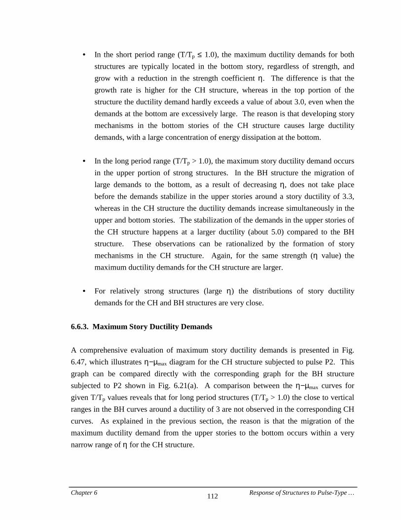
Chapter 6 Response of Structures to Pulse-Type … 112
• = In the short period range (T/Tp ≤ 1.0), the maximum ductility demands for both structures are typically located in the bottom story, regardless of strength, and grow with a reduction in the strength coefficient η. The difference is that the growth rate is higher for the CH structure, whereas in the top portion of the structure the ductility demand hardly exceeds a value of about 3.0, even when the demands at the bottom are excessively large. The reason is that developing story mechanisms in the bottom stories of the CH structure causes large ductility demands, with a large concentration of energy dissipation at the bottom.
• = In the long period range (T/Tp > 1.0), the maximum story ductility demand occurs
in the upper portion of strong structures. In the BH structure the migration of large demands to the bottom, as a result of decreasing η, does not take place before the demands stabilize in the upper stories around a story ductility of 3.3, whereas in the CH structure the ductility demands increase simultaneously in the upper and bottom stories. The stabilization of the demands in the upper stories of the CH structure happens at a larger ductility (about 5.0) compared to the BH structure. These observations can be rationalized by the formation of story mechanisms in the CH structure. Again, for the same strength (η value) the maximum ductility demands for the CH structure are larger.
• = For relatively strong structures (large η) the distributions of story ductility
demands for the CH and BH structures are very close. 6.6.3. Maximum Story Ductility Demands A comprehensive evaluation of maximum story ductility demands is presented in Fig. 6.47, which illustrates η−µmax diagram for the CH structure subjected to pulse P2. This graph can be compared directly with the corresponding graph for the BH structure subjected to P2 shown in Fig. 6.21(a). A comparison between the η−µmax curves for given T/Tp values reveals that for long period structures (T/Tp > 1.0) the close to vertical ranges in the BH curves around a ductility of 3 are not observed in the corresponding CH curves. As explained in the previous section, the reason is that the migration of the maximum ductility demand from the upper stories to the bottom occurs within a very narrow range of η for the CH structure.
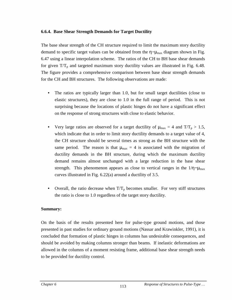
Chapter 6 Response of Structures to Pulse-Type … 113
6.6.4. Base Shear Strength Demands for Target Ductility The base shear strength of the CH structure required to limit the maximum story ductility demand to specific target values can be obtained from the η−µmax diagram shown in Fig. 6.47 using a linear interpolation scheme. The ratios of the CH to BH base shear demands for given T/Tp and targeted maximum story ductility values are illustrated in Fig. 6.48. The figure provides a comprehensive comparison between base shear strength demands for the CH and BH structures. The following observations are made:
• = The ratios are typically larger than 1.0, but for small target ductilities (close to elastic structures), they are close to 1.0 in the full range of period. This is not surprising because the locations of plastic hinges do not have a significant effect on the response of strong structures with close to elastic behavior.
• = Very large ratios are observed for a target ductility of µmax = 4 and T/Tp > 1.5,
which indicate that in order to limit story ductility demands to a target value of 4, the CH structure should be several times as strong as the BH structure with the same period. The reason is that µmax = 4 is associated with the migration of ductility demands in the BH structure, during which the maximum ductility demand remains almost unchanged with a large reduction in the base shear strength. This phenomenon appears as close to vertical ranges in the 1/η−µmax curves illustrated in Fig. 6.22(a) around a ductility of 3.5.
• = Overall, the ratio decrease when T/Tp becomes smaller. For very stiff structures
the ratio is close to 1.0 regardless of the target story ductility. Summary: On the basis of the results presented here for pulse-type ground motions, and those presented in past studies for ordinary ground motions (Nassar and Krawinkler, 1991), it is concluded that formation of plastic hinges in columns has undesirable consequences, and should be avoided by making columns stronger than beams. If inelastic deformations are allowed in the columns of a moment resisting frame, additional base shear strength needs to be provided for ductility control.
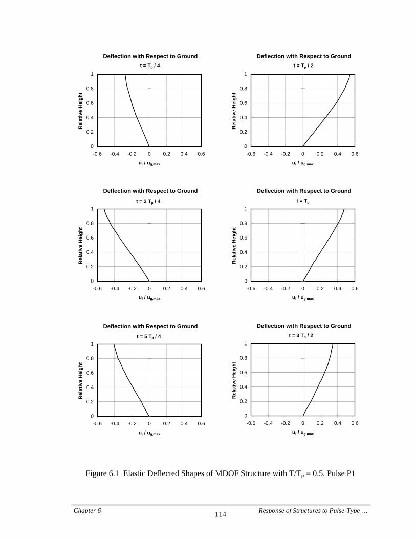
Chapter 6 Response of Structures to Pulse-Type … 114
Deflection with Respect to Ground
0
0.2
0.4
0.6
0.8
1
-0.6 -0.4 -0.2 0 0.2 0.4 0.6
ui / ug,max
Rel
ativ
e H
eigh
t
t = Tp / 4Deflection with Respect to Ground
0
0.2
0.4
0.6
0.8
1
-0.6 -0.4 -0.2 0 0.2 0.4 0.6
ui / ug,max
Rel
ativ
e H
eigh
t
t = Tp / 2
Deflection with Respect to Ground
0
0.2
0.4
0.6
0.8
1
-0.6 -0.4 -0.2 0 0.2 0.4 0.6
ui / ug,max
Rel
ativ
e H
eigh
t
t = 3 Tp / 4
Deflection with Respect to Ground
0
0.2
0.4
0.6
0.8
1
-0.6 -0.4 -0.2 0 0.2 0.4 0.6
ui / ug,max
Rel
ativ
e H
eigh
t
t = Tp
Deflection with Respect to Ground
0
0.2
0.4
0.6
0.8
1
-0.6 -0.4 -0.2 0 0.2 0.4 0.6
ui / ug,max
Rel
ativ
e H
eigh
t
t = 5 Tp / 4
Deflection with Respect to Ground
0
0.2
0.4
0.6
0.8
1
-0.6 -0.4 -0.2 0 0.2 0.4 0.6
ui / ug,max
Rel
ativ
e H
eigh
t
t = 3 Tp / 2
Figure 6.1 Elastic Deflected Shapes of MDOF Structure with T/Tp = 0.5, Pulse P1

Chapter 6 Response of Structures to Pulse-Type … 115
Deflection with Respect to Ground
0
0.2
0.4
0.6
0.8
1
-1.4 -1 -0.6 -0.2 0.2 0.6 1 1.4
ui / ug,max
Rel
ativ
e H
eigh
t
t = Tp / 4Deflection with Respect to Ground
0
0.2
0.4
0.6
0.8
1
-1.4 -1 -0.6 -0.2 0.2 0.6 1 1.4
ui / ug,max
Rel
ativ
e H
eigh
t
t = Tp / 2
Deflection with Respect to Ground
0
0.2
0.4
0.6
0.8
1
-1.4 -1 -0.6 -0.2 0.2 0.6 1 1.4
ui / ug,max
Rel
ativ
e H
eigh
t
t = 3 Tp / 4Deflection with Respect to Ground
0
0.2
0.4
0.6
0.8
1
-1.4 -1 -0.6 -0.2 0.2 0.6 1 1.4
ui / ug,max
Rel
ativ
e H
eigh
t
t = Tp
Deflection with Respect to Ground
0
0.2
0.4
0.6
0.8
1
-1.4 -1 -0.6 -0.2 0.2 0.6 1 1.4
ui / ug,max
Rel
ativ
e H
eigh
t
t = 5 Tp / 4Deflection with Respect to Ground
0
0.2
0.4
0.6
0.8
1
-1.4 -1 -0.6 -0.2 0.2 0.6 1 1.4
ui / ug,max
Rel
ativ
e H
eigh
t
t = 3 Tp / 2
Figure 6.2 Elastic Deflected Shapes of MDOF Structure with T/Tp = 2.0, Pulse P1
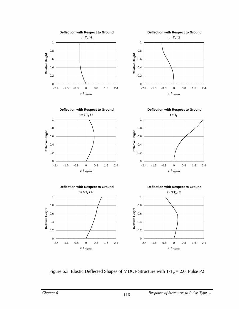
Chapter 6 Response of Structures to Pulse-Type … 116
Deflection with Respect to Ground
0
0.2
0.4
0.6
0.8
1
-2.4 -1.6 -0.8 0 0.8 1.6 2.4
ui / ug,max
Rel
ativ
e H
eigh
t
t = Tp / 4Deflection with Respect to Ground
0
0.2
0.4
0.6
0.8
1
-2.4 -1.6 -0.8 0 0.8 1.6 2.4
ui / ug,max
Rel
ativ
e H
eigh
t
t = Tp / 2
Deflection with Respect to Ground
0
0.2
0.4
0.6
0.8
1
-2.4 -1.6 -0.8 0 0.8 1.6 2.4
ui / ug,max
Rel
ativ
e H
eigh
t
t = 3 Tp / 4Deflection with Respect to Ground
0
0.2
0.4
0.6
0.8
1
-2.4 -1.6 -0.8 0 0.8 1.6 2.4
ui / ug,max
Rel
ativ
e H
eigh
t
t = Tp
Deflection with Respect to Ground
0
0.2
0.4
0.6
0.8
1
-2.4 -1.6 -0.8 0 0.8 1.6 2.4
ui / ug,max
Rel
ativ
e H
eigh
t
t = 5 Tp / 4Deflection with Respect to Ground
0
0.2
0.4
0.6
0.8
1
-2.4 -1.6 -0.8 0 0.8 1.6 2.4
ui / ug,max
Rel
ativ
e H
eigh
t
t = 3 Tp / 2
Figure 6.3 Elastic Deflected Shapes of MDOF Structure with T/Tp = 2.0, Pulse P2
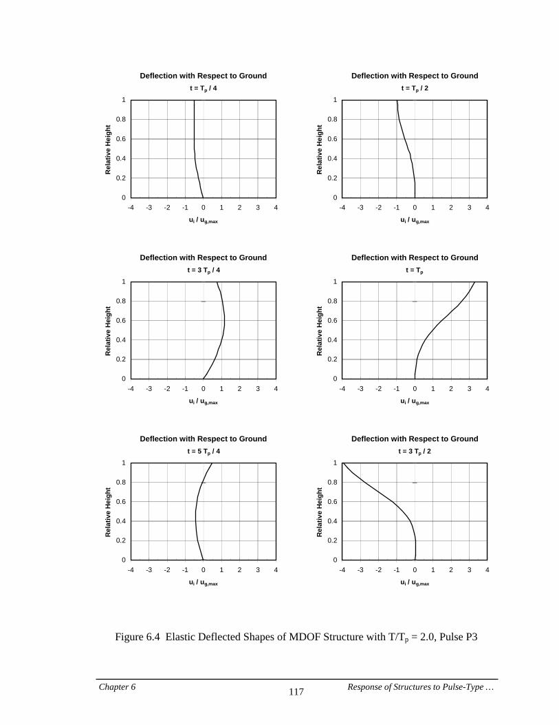
Chapter 6 Response of Structures to Pulse-Type … 117
Deflection with Respect to Ground
0
0.2
0.4
0.6
0.8
1
-4 -3 -2 -1 0 1 2 3 4
ui / ug,max
Rel
ativ
e H
eigh
t
t = Tp / 4Deflection with Respect to Ground
0
0.2
0.4
0.6
0.8
1
-4 -3 -2 -1 0 1 2 3 4
ui / ug,max
Rel
ativ
e H
eigh
t
t = Tp / 2
Deflection with Respect to Ground
0
0.2
0.4
0.6
0.8
1
-4 -3 -2 -1 0 1 2 3 4
ui / ug,max
Rel
ativ
e H
eigh
t
t = 3 Tp / 4Deflection with Respect to Ground
0
0.2
0.4
0.6
0.8
1
-4 -3 -2 -1 0 1 2 3 4
ui / ug,max
Rel
ativ
e H
eigh
t
t = Tp
Deflection with Respect to Ground
0
0.2
0.4
0.6
0.8
1
-4 -3 -2 -1 0 1 2 3 4
ui / ug,max
Rel
ativ
e H
eigh
t
t = 5 Tp / 4Deflection with Respect to Ground
0
0.2
0.4
0.6
0.8
1
-4 -3 -2 -1 0 1 2 3 4
ui / ug,max
Rel
ativ
e H
eigh
t
t = 3 Tp / 2
Figure 6.4 Elastic Deflected Shapes of MDOF Structure with T/Tp = 2.0, Pulse P3
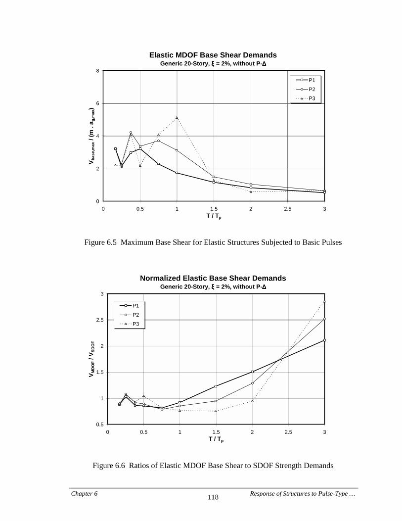
Chapter 6 Response of Structures to Pulse-Type … 118
Elastic MDOF Base Shear DemandsGeneric 20-Story, ξξξξ = 2%, without P-∆∆∆∆
0
2
4
6
8
0 0.5 1 1.5 2 2.5 3T / Tp
V bas
e,m
ax /
(m .
a g,m
ax)
P1
P2
P3
Figure 6.5 Maximum Base Shear for Elastic Structures Subjected to Basic Pulses
Normalized Elastic Base Shear DemandsGeneric 20-Story, ξξξξ = 2%, without P-∆∆∆∆
0.5
1
1.5
2
2.5
3
0 0.5 1 1.5 2 2.5 3T / Tp
V MD
OF /
VSD
OF
P1
P2
P3
Figure 6.6 Ratios of Elastic MDOF Base Shear to SDOF Strength Demands
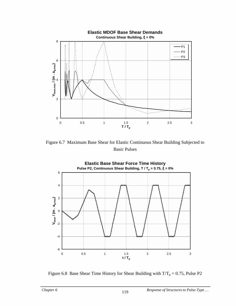
Chapter 6 Response of Structures to Pulse-Type … 119
Elastic MDOF Base Shear DemandsContinuous Shear Building, ξξξξ = 0%
0
2
4
6
8
0 0.5 1 1.5 2 2.5 3T / Tp
V bas
e,m
ax /
(m .
a g,m
ax)
P1P2P3
Figure 6.7 Maximum Base Shear for Elastic Continuous Shear Building Subjected to Basic Pulses
Elastic Base Shear Force Time History
Pulse P2, Continuous Shear Building, T / Tp = 0.75, ξξξξ = 0%
-6
-4
-2
0
2
4
6
0 0.5 1 1.5 2 2.5 3t / Tp
V bas
e / (m
. a g
,max
)
Figure 6.8 Base Shear Time History for Shear Building with T/Tp = 0.75, Pulse P2
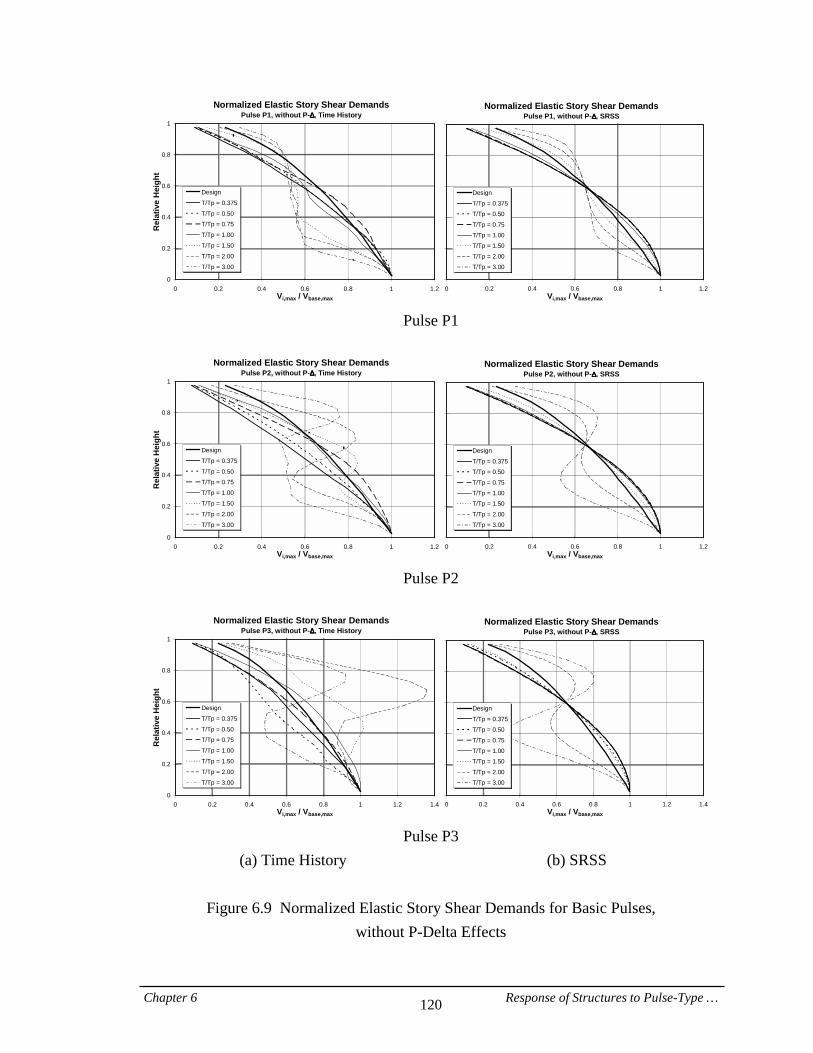
Chapter 6 Response of Structures to Pulse-Type … 120
Normalized Elastic Story Shear DemandsPulse P1, without P-∆∆∆∆, Time History
0
0.2
0.4
0.6
0.8
1
0 0.2 0.4 0.6 0.8 1 1.2Vi,max / Vbase,max
Rel
ativ
e H
eigh
t
DesignT/Tp = 0.375T/Tp = 0.50T/Tp = 0.75T/Tp = 1.00T/Tp = 1.50T/Tp = 2.00T/Tp = 3.00
Normalized Elastic Story Shear DemandsPulse P1, without P-∆∆∆∆, SRSS
0 0.2 0.4 0.6 0.8 1 1.2Vi,max / Vbase,max
Design
T/Tp = 0.375T/Tp = 0.50
T/Tp = 0.75T/Tp = 1.00T/Tp = 1.50
T/Tp = 2.00T/Tp = 3.00
Pulse P1
Normalized Elastic Story Shear Demands
Pulse P2, without P-∆∆∆∆, Time History
0
0.2
0.4
0.6
0.8
1
0 0.2 0.4 0.6 0.8 1 1.2Vi,max / Vbase,max
Rel
ativ
e H
eigh
t
Design
T/Tp = 0.375
T/Tp = 0.50T/Tp = 0.75
T/Tp = 1.00
T/Tp = 1.50
T/Tp = 2.00
T/Tp = 3.00
Normalized Elastic Story Shear DemandsPulse P2, without P-∆∆∆∆, SRSS
0 0.2 0.4 0.6 0.8 1 1.2Vi,max / Vbase,max
Design
T/Tp = 0.375T/Tp = 0.50
T/Tp = 0.75T/Tp = 1.00T/Tp = 1.50
T/Tp = 2.00T/Tp = 3.00
Pulse P2
Normalized Elastic Story Shear Demands
Pulse P3, without P-∆∆∆∆, Time History
0
0.2
0.4
0.6
0.8
1
0 0.2 0.4 0.6 0.8 1 1.2 1.4Vi,max / Vbase,max
Rel
ativ
e H
eigh
t
Design
T/Tp = 0.375
T/Tp = 0.50T/Tp = 0.75
T/Tp = 1.00
T/Tp = 1.50
T/Tp = 2.00
T/Tp = 3.00
Normalized Elastic Story Shear DemandsPulse P3, without P-∆∆∆∆, SRSS
0 0.2 0.4 0.6 0.8 1 1.2 1.4Vi,max / Vbase,max
Design
T/Tp = 0.375T/Tp = 0.50
T/Tp = 0.75T/Tp = 1.00T/Tp = 1.50
T/Tp = 2.00T/Tp = 3.00
Pulse P3
(a) Time History (b) SRSS
Figure 6.9 Normalized Elastic Story Shear Demands for Basic Pulses, without P-Delta Effects
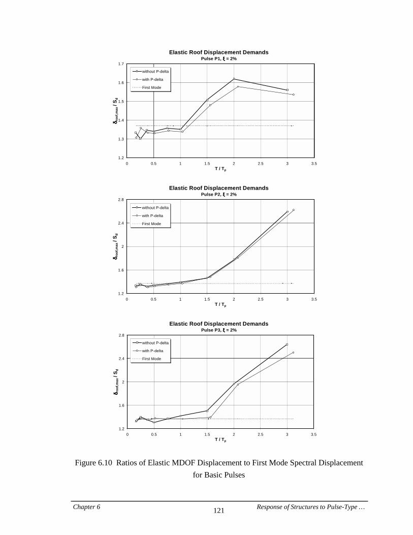
Chapter 6 Response of Structures to Pulse-Type … 121
Elastic Roof Displacement DemandsPulse P1, ξξξξ = 2%
1.2
1.3
1.4
1.5
1.6
1.7
0 0.5 1 1.5 2 2.5 3 3.5T / Tp
δδ δδ roo
f,max
/ S d
without P-delta
with P-delta
First Mode
Elastic Roof Displacement DemandsPulse P2, ξξξξ = 2%
1.2
1.6
2
2.4
2.8
0 0.5 1 1.5 2 2.5 3 3.5T / Tp
δδ δδ roo
f,max
/ S d
without P-delta
with P-delta
First Mode
Elastic Roof Displacement DemandsPulse P3, ξξξξ = 2%
1.2
1.6
2
2.4
2.8
0 0.5 1 1.5 2 2.5 3 3.5T / Tp
δδ δδ roo
f,max
/ S d
without P-delta
with P-delta
First Mode
Figure 6.10 Ratios of Elastic MDOF Displacement to First Mode Spectral Displacement for Basic Pulses
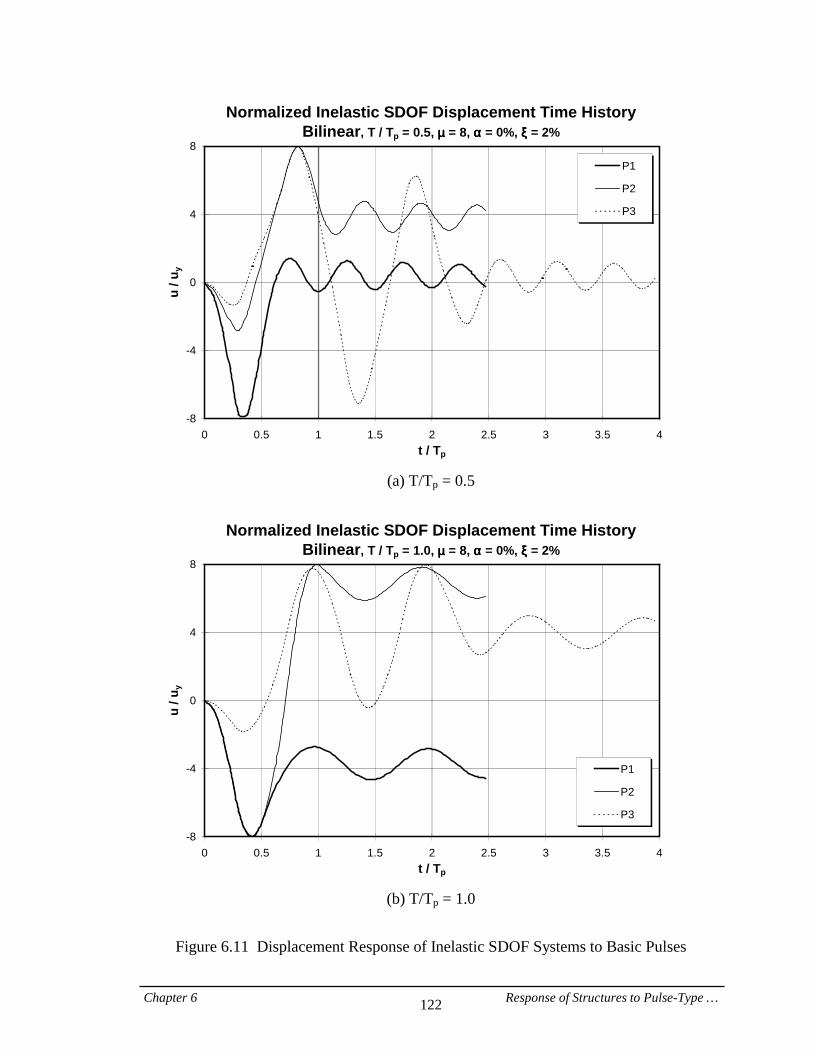
Chapter 6 Response of Structures to Pulse-Type … 122
Normalized Inelastic SDOF Displacement Time HistoryBilinear, T / Tp = 0.5, µµµµ = 8, αααα = 0%, ξξξξ = 2%
-8
-4
0
4
8
0 0.5 1 1.5 2 2.5 3 3.5 4t / Tp
u / u
y P1
P2
P3
(a) T/Tp = 0.5
Normalized Inelastic SDOF Displacement Time History
Bilinear, T / Tp = 1.0, µµµµ = 8, αααα = 0%, ξξξξ = 2%
-8
-4
0
4
8
0 0.5 1 1.5 2 2.5 3 3.5 4t / Tp
u / u
y
P1
P2
P3
(b) T/Tp = 1.0
Figure 6.11 Displacement Response of Inelastic SDOF Systems to Basic Pulses
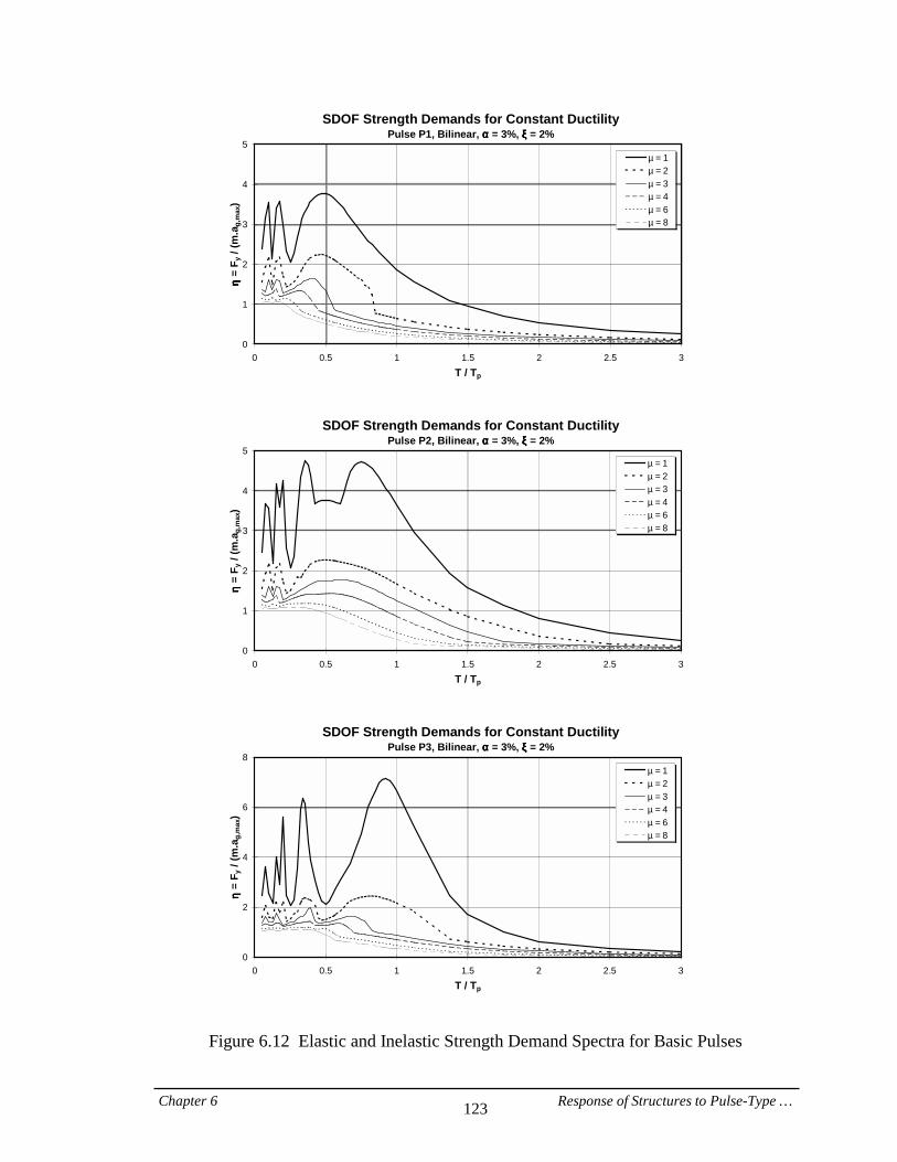
Chapter 6 Response of Structures to Pulse-Type … 123
SDOF Strength Demands for Constant DuctilityPulse P1, Bilinear, αααα = 3%, ξξξξ = 2%
0
1
2
3
4
5
0 0.5 1 1.5 2 2.5 3T / Tp
ηη ηη =
F y /
(m.a
g,m
ax)
µ===1µ===2µ===3µ===4µ===6µ===8
SDOF Strength Demands for Constant DuctilityPulse P2, Bilinear, αααα = 3%, ξξξξ = 2%
0
1
2
3
4
5
0 0.5 1 1.5 2 2.5 3T / Tp
ηη ηη =
F y /
(m.a
g,m
ax)
µ===1µ===2µ===3µ===4µ===6µ===8
SDOF Strength Demands for Constant DuctilityPulse P3, Bilinear, αααα = 3%, ξξξξ = 2%
0
2
4
6
8
0 0.5 1 1.5 2 2.5 3T / Tp
ηη ηη =
F y /
(m.a
g,m
ax)
µ===1µ===2µ===3µ===4µ===6µ===8
Figure 6.12 Elastic and Inelastic Strength Demand Spectra for Basic Pulses
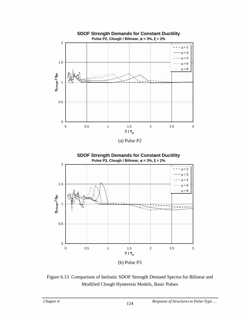
Chapter 6 Response of Structures to Pulse-Type … 124
SDOF Strength Demands for Constant DuctilityPulse P2, Clough / Bilinear, αααα = 3%, ξξξξ = 2%
0
0.5
1
1.5
2
0 0.5 1 1.5 2 2.5 3T / Tp
ηη ηη Clo
ugh== ==
// // == == ηη ηηB
i
µ===2
µ===3
µ===4
µ===6
µ===8
(a) Pulse P2
SDOF Strength Demands for Constant Ductility
Pulse P3, Clough / Bilinear, αααα = 3%, ξξξξ = 2%
0
0.5
1
1.5
2
0 0.5 1 1.5 2 2.5 3T / Tp
ηη ηη Clo
ugh== ==
// // == == ηη ηηB
i
µ===2
µ===3
µ===4
µ===6
µ===8
(b) Pulse P3
Figure 6.13 Comparison of Inelastic SDOF Strength Demand Spectra for Bilinear and
Modified Clough Hysteresis Models, Basic Pulses

Chapter 6 Response of Structures to Pulse-Type … 125
SDOF Ductility DemandsPulse P1, Bilinear, αααα = 3%, ξξξξ = 2%
0
0.4
0.8
1.2
1.6
2
0 4 8 12 16 20
Ductility,,,,====µµµµ
ηη ηη =
F y /
(m.a
g,m
ax)
T/Tp = 0.375T/Tp = 0.50T/Tp = 0.75T/Tp = 1.00T/Tp = 1.50T/Tp = 2.00T/Tp = 3.00
Figure 6.14 Ductility Demands for SDOF Systems Subjected to Pulse P1
SDOF Ductility DemandsPulse P2, Bilinear, αααα = 3%, ξξξξ = 2%
0
0.4
0.8
1.2
1.6
2
0 4 8 12 16 20
Ductility,,,,====µµµµ
ηη ηη =
F y /
(m.a
g,m
ax)
T/Tp = 0.375T/Tp = 0.50T/Tp = 0.75T/Tp = 1.00T/Tp = 1.50T/Tp = 2.00T/Tp = 3.00
Figure 6.15 Ductility Demands for SDOF Systems Subjected to Pulse P2
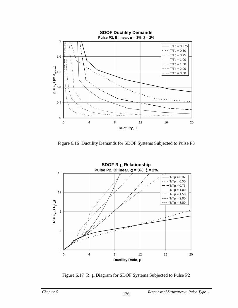
Chapter 6 Response of Structures to Pulse-Type … 126
SDOF Ductility DemandsPulse P3, Bilinear, αααα = 3%, ξξξξ = 2%
0
0.4
0.8
1.2
1.6
2
0 4 8 12 16 20
Ductility,,,,====µµµµ
ηη ηη =
F y /
(m.a
g,m
ax)
T/Tp = 0.375T/Tp = 0.50T/Tp = 0.75T/Tp = 1.00T/Tp = 1.50T/Tp = 2.00T/Tp = 3.00
Figure 6.16 Ductility Demands for SDOF Systems Subjected to Pulse P3
SDOF R-µµµµ RelationshipPulse P2, Bilinear, αααα = 3%, ξξξξ = 2%
0
4
8
12
16
0 4 8 12 16 20
Ductility Ratio, µµµµ
R =
Fy,
e / F
y( µµ µµ)
T/Tp = 0.375T/Tp = 0.50T/Tp = 0.75T/Tp = 1.00T/Tp = 1.50T/Tp = 2.00T/Tp = 3.00
Figure 6.17 R−µ Diagram for SDOF Systems Subjected to Pulse P2
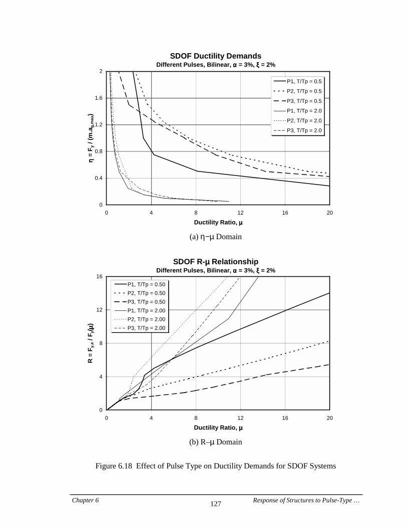
Chapter 6 Response of Structures to Pulse-Type … 127
SDOF Ductility DemandsDifferent Pulses, Bilinear, αααα = 3%, ξξξξ = 2%
0
0.4
0.8
1.2
1.6
2
0 4 8 12 16 20
Ductility Ratio,,,,====µµµµ
ηη ηη =
F y /
(m.a
g,m
ax)
P1, T/Tp = 0.5
P2, T/Tp = 0.5
P3, T/Tp = 0.5
P1, T/Tp = 2.0
P2, T/Tp = 2.0
P3, T/Tp = 2.0
(a) η−µ Domain
SDOF R-µµµµ Relationship
Different Pulses, Bilinear, αααα = 3%, ξξξξ = 2%
0
4
8
12
16
0 4 8 12 16 20
Ductility Ratio, µµµµ
R =
Fy,
e / F
y( µµ µµ)
P1, T/Tp = 0.50P2, T/Tp = 0.50P3, T/Tp = 0.50P1, T/Tp = 2.00P2, T/Tp = 2.00P3, T/Tp = 2.00
(b) R–µ=Domain
Figure 6.18 Effect of Pulse Type on Ductility Demands for SDOF Systems
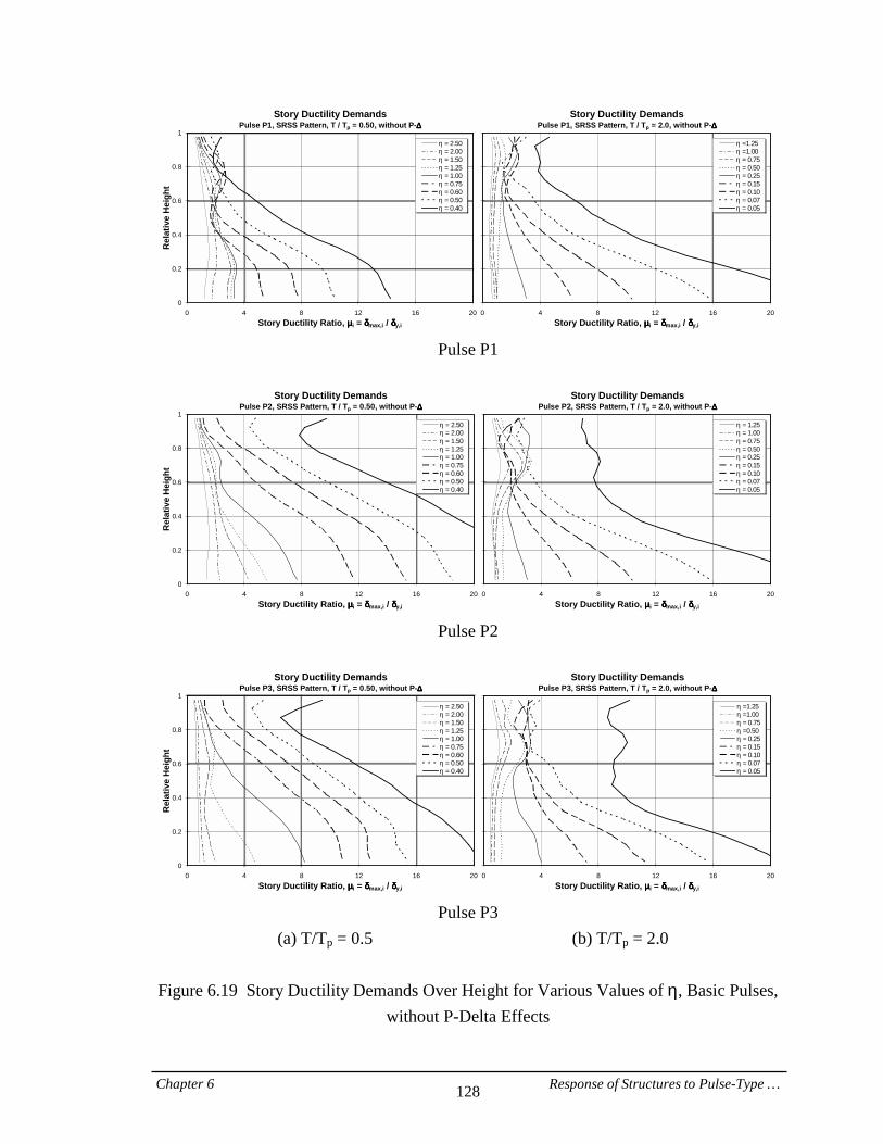
Chapter 6 Response of Structures to Pulse-Type … 128
Story Ductility DemandsPulse P1, SRSS Pattern, T / Tp = 0.50, without P-∆∆∆∆
0
0.2
0.4
0.6
0.8
1
0 4 8 12 16 20Story Ductility Ratio, µµµµi = δδδδmax,i / δδδδy,i
Rel
ativ
e H
eigh
t
η===2.50η===2.00η===1.50η===1.25η===1.00η===0.75η===0.60η===0.50η===0.40
Story Ductility DemandsPulse P1, SRSS Pattern, T / Tp = 2.0, without P-∆∆∆∆
0 4 8 12 16 20Story Ductility Ratio, µµµµi = δδδδmax,i / δδδδy,i
η==1.25η==1.00η===0.75η===0.50η===0.25η===0.15η===0.10η===0.07η===0.05
Pulse P1
Story Ductility Demands
Pulse P2, SRSS Pattern, T / Tp = 0.50, without P-∆∆∆∆
0
0.2
0.4
0.6
0.8
1
0 4 8 12 16 20Story Ductility Ratio, µµµµi = δδδδmax,i / δδδδy,i
Rel
ativ
e H
eigh
t
η===2.50η===2.00η===1.50η===1.25η===1.00η===0.75η===0.60η===0.50η===0.40
Story Ductility DemandsPulse P2, SRSS Pattern, T / Tp = 2.0, without P-∆∆∆∆
0 4 8 12 16 20Story Ductility Ratio, µµµµi = δδδδmax,i / δδδδy,i
η===1.25η===1.00η===0.75η===0.50η===0.25η===0.15η===0.10η===0.07η===0.05
Pulse P2
Story Ductility Demands
Pulse P3, SRSS Pattern, T / Tp = 0.50, without P-∆∆∆∆
0
0.2
0.4
0.6
0.8
1
0 4 8 12 16 20Story Ductility Ratio, µµµµi = δδδδmax,i / δδδδy,i
Rel
ativ
e H
eigh
t
η===2.50η===2.00η===1.50η===1.25η===1.00η===0.75η===0.60η===0.50η===0.40
Story Ductility DemandsPulse P3, SRSS Pattern, T / Tp = 2.0, without P-∆∆∆∆
0 4 8 12 16 20Story Ductility Ratio, µµµµi = δδδδmax,i / δδδδy,i
η==1.25η==1.00η===0.75η==0.50η===0.25η===0.15η===0.10η===0.07η===0.05
Pulse P3
(a) T/Tp = 0.5 (b) T/Tp = 2.0
Figure 6.19 Story Ductility Demands Over Height for Various Values of η, Basic Pulses, without P-Delta Effects
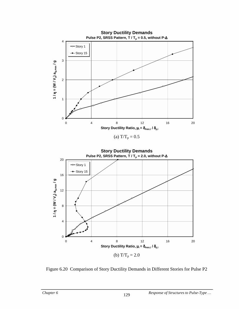
Chapter 6 Response of Structures to Pulse-Type … 129
Story Ductility DemandsPulse P2, SRSS Pattern, T / Tp = 0.5, without P-∆∆∆∆
0
1
2
3
4
0 4 8 12 16 20Story Ductility Ratio,,,,====µµµµi = δδδδmax,i / δδδδy,i
1 / ηη ηη
= (W
/ V y
) ag,
max
/ g
Story 1
Story 15
(a) T/Tp = 0.5
Story Ductility Demands
Pulse P2, SRSS Pattern, T / Tp = 2.0, without P-∆∆∆∆
0
4
8
12
16
20
0 4 8 12 16 20Story Ductility Ratio,,,,====µµµµi = δδδδmax,i / δδδδy,i
1 / ηη ηη
= (W
/ V y
) ag,
max
/ g
Story 1
Story 15
(b) T/Tp = 2.0
Figure 6.20 Comparison of Story Ductility Demands in Different Stories for Pulse P2
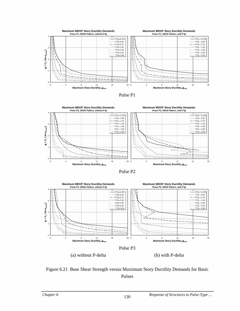
Chapter 6 Response of Structures to Pulse-Type … 130
Maximum MDOF Story Ductility DemandsPulse P1, SRSS Pattern, without P-∆∆∆∆
0
1
2
3
4
0 4 8 12 16 20Maximum Story Ductility,,,,====µµµµmax
ηη ηη =
V y /
(m.a
g,m
ax)
T/Tp=0.375T/Tp=0.50T/Tp=0.75T/Tp=1.00T/Tp=1.50T/Tp=2.00 T/Tp=3.00
Maximum MDOF Story Ductility DemandsPulse P1, SRSS Pattern, with P-∆∆∆∆
0 4 8 12 16 20Maximum Story Ductility,,,,====µµµµmax
T/Tp = 0.375T/Tp = 0.50T/Tp = 0.75T/Tp = 1.00T/Tp = 1.50T/Tp = 2.00T/Tp = 3.00
Pulse P1
Maximum MDOF Story Ductility Demands
Pulse P2, SRSS Pattern, without P-∆∆∆∆
0
1
2
3
4
0 4 8 12 16 20Maximum Story Ductility,,,,====µµµµmax
ηη ηη =
V y /
(m.a
g,m
ax)
T/Tp = 0.375T/Tp = 0.50T/Tp = 0.75T/Tp = 1.00T/Tp = 1.50T/Tp = 2.00T/Tp = 3.00
Maximum MDOF Story Ductility DemandsPulse P2, SRSS Pattern, with P-∆∆∆∆
0 4 8 12 16 20Maximum Story Ductility,,,,====µµµµmax
T/Tp = 0.375T/Tp = 0.50T/Tp = 0.75T/Tp = 1.00T/Tp = 1.50T/Tp = 2.00T/Tp = 3.00
Pulse P2
Maximum MDOF Story Ductility Demands
Pulse P3, SRSS Pattern, without P-∆∆∆∆
0
1
2
3
4
0 4 8 12 16 20Maximum Story Ductility,,,,====µµµµmax
ηη ηη =
V y /
(m.a
g,m
ax)
T/Tp=0.375T/Tp=0.50T/Tp=0.75T/Tp=1.00T/Tp=1.50T/Tp=2.00 T/Tp=3.00
Maximum MDOF Story Ductility DemandsPulse P3, SRSS Pattern, with P-∆∆∆∆
0 4 8 12 16 20Maximum Story Ductility,,,,====µµµµmax
T/Tp = 0.375T/Tp = 0.50T/Tp = 0.75T/Tp = 1.00T/Tp = 1.50T/Tp = 2.00T/Tp = 3.00
Pulse P3
(a) without P-delta (b) with P-delta
Figure 6.21 Base Shear Strength versus Maximum Story Ductility Demands for Basic Pulses

Chapter 6 Response of Structures to Pulse-Type … 131
Maximum MDOF Story Ductility DemandsPulse P2, SRSS Pattern, without P-∆∆∆∆
0
4
8
12
16
20
0 4 8 12 16 20Maximum Story Ductility,,,,====µµµµmax
1 / ηη ηη
= (W
/ V y
) ag,
max
/ g
T/Tp = 0.375T/Tp = 0.50T/Tp = 0.75T/Tp = 1.00T/Tp = 1.50T/Tp = 2.00T/Tp = 3.00
(a) without P-delta
Maximum MDOF Story Ductility Demands
Pulse P2, SRSS Pattern, with P-∆∆∆∆
0
4
8
12
16
20
0 4 8 12 16 20Maximum Story Ductility,,,,====µµµµmax
1 / ηη ηη
= (W
/ V y
) ag,
max
/ g
T/Tp = 0.375T/Tp = 0.50T/Tp = 0.75T/Tp = 1.00T/Tp = 1.50T/Tp = 2.00T/Tp = 3.00
(b) with P-delta
Figure 6.22 1/η−µmax Diagrams for MDOF Structures Subjected to Pulse P2
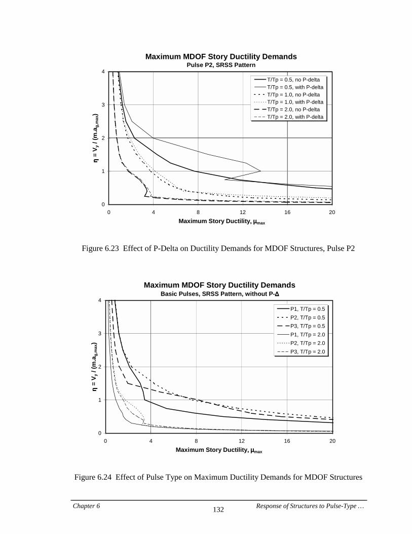
Chapter 6 Response of Structures to Pulse-Type … 132
Maximum MDOF Story Ductility DemandsPulse P2, SRSS Pattern
0
1
2
3
4
0 4 8 12 16 20Maximum Story Ductility,,,,====µµµµmax
ηη ηη =
V y /
(m.a
g,m
ax)
T/Tp = 0.5, no P-deltaT/Tp = 0.5, with P-deltaT/Tp = 1.0, no P-deltaT/Tp = 1.0, with P-deltaT/Tp = 2.0, no P-deltaT/Tp = 2.0, with P-delta
Figure 6.23 Effect of P-Delta on Ductility Demands for MDOF Structures, Pulse P2
Maximum MDOF Story Ductility DemandsBasic Pulses, SRSS Pattern, without P-∆∆∆∆
0
1
2
3
4
0 4 8 12 16 20Maximum Story Ductility,,,,====µµµµmax
ηη ηη =
V y /
(m.a
g,m
ax)
P1, T/Tp = 0.5P2, T/Tp = 0.5P3, T/Tp = 0.5P1, T/Tp = 2.0P2, T/Tp = 2.0P3, T/Tp = 2.0
Figure 6.24 Effect of Pulse Type on Maximum Ductility Demands for MDOF Structures
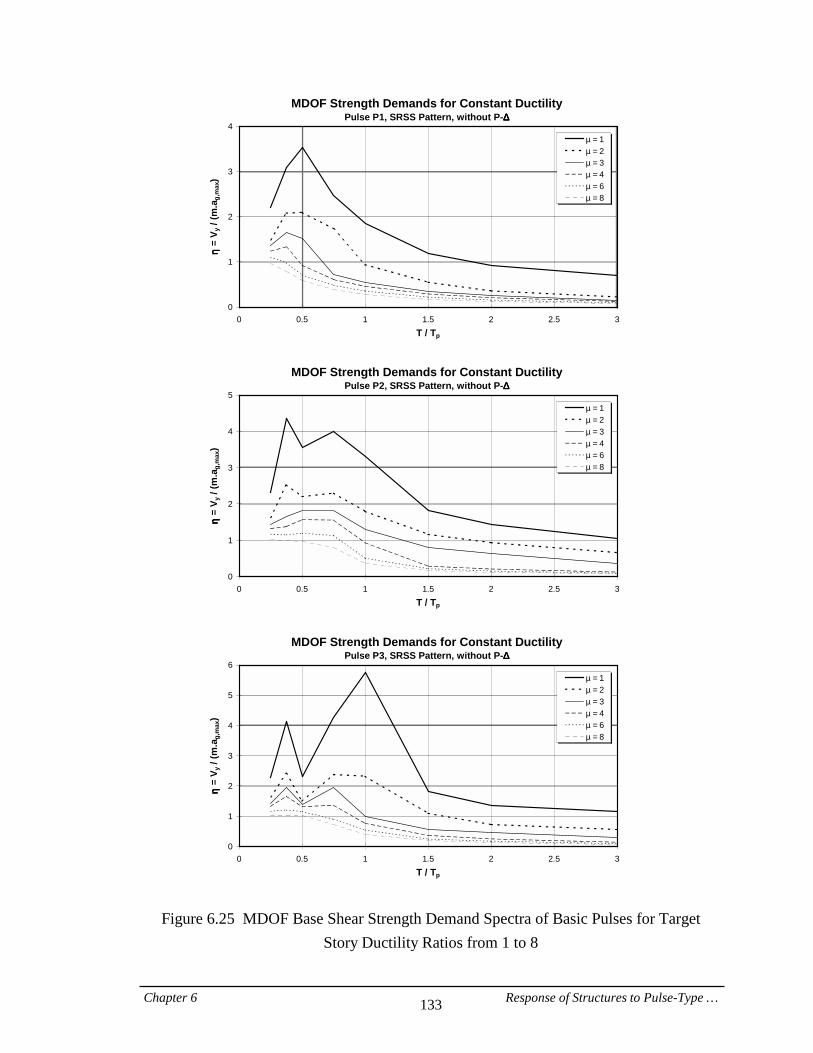
Chapter 6 Response of Structures to Pulse-Type … 133
MDOF Strength Demands for Constant DuctilityPulse P1, SRSS Pattern, without P-∆∆∆∆
0
1
2
3
4
0 0.5 1 1.5 2 2.5 3T / Tp
ηη ηη =
V y /
(m.a
g,m
ax)
µ===1µ===2µ===3µ===4µ===6µ===8
MDOF Strength Demands for Constant DuctilityPulse P2, SRSS Pattern, without P-∆∆∆∆
0
1
2
3
4
5
0 0.5 1 1.5 2 2.5 3T / Tp
ηη ηη =
V y /
(m.a
g,m
ax)
µ===1µ===2µ===3µ===4µ===6µ===8
MDOF Strength Demands for Constant DuctilityPulse P3, SRSS Pattern, without P-∆∆∆∆
0
1
2
3
4
5
6
0 0.5 1 1.5 2 2.5 3T / Tp
ηη ηη =
V y /
(m.a
g,m
ax)
µ===1µ===2µ===3µ===4µ===6µ===8
Figure 6.25 MDOF Base Shear Strength Demand Spectra of Basic Pulses for Target Story Ductility Ratios from 1 to 8

Chapter 6 Response of Structures to Pulse-Type … 134
Strength Demand Ratios for Constant DuctilityPulse P1, SRSS Pattern
0
1
2
3
4
5
0 0.5 1 1.5 2 2.5 3T / Tp
ηη ηη MD
OF== ==
// // == == ηη ηηSD
OF
µ===1µ===2µ===3µ===4µ===6µ===8
Strength Demand Ratios for Constant DuctilityPulse P2, SRSS Pattern
0
1
2
3
4
5
0 0.5 1 1.5 2 2.5 3T / Tp
ηη ηη MD
OF== ==
// // == == ηη ηηSD
OF
µ===1µ===2µ===3µ===4µ===6µ===8
Strength Demand Ratios for Constant DuctilityPulse P3, SRSS Pattern
0
1
2
3
4
5
0 0.5 1 1.5 2 2.5 3T / Tp
ηη ηη MD
OF== ==
// // == == ηη ηηSD
OF
µ===1µ===2µ===3µ===4µ===6µ===8
Figure 6.26 Ratios of MDOF to SDOF Strength Demands for Basic Pulses

Chapter 6 Response of Structures to Pulse-Type … 135
MDOF Strength Demand Ratios for Constant DuctilityPulse P1, SRSS Pattern
0.6
1
1.4
1.8
2.2
0 0.5 1 1.5 2 2.5 3T / Tp
ηη ηη (( ((P −
∆)−∆
)−∆
)−∆
)== ==// // == == ηη ηη
(( ((no
P −∆)
−∆)
−∆)
−∆)
µ===1µ===2µ===3µ===4µ===6µ===8
MDOF Strength Demand Ratios for Constant DuctilityPulse P2, SRSS Pattern
0.6
1
1.4
1.8
2.2
0 0.5 1 1.5 2 2.5 3T / Tp
ηη ηη (( ((P −
∆)−∆
)−∆
)−∆
)== ==// // == == ηη ηη
(( ((no
P −∆)
−∆)
−∆)
−∆)
µ===1µ===2µ===3µ===4µ===6µ===8
MDOF Strength Demand Ratios for Constant DuctilityPulse P3, SRSS Pattern
0.6
1
1.4
1.8
2.2
0 0.5 1 1.5 2 2.5 3T / Tp
ηη ηη (( ((P −
∆)−∆
)−∆
)−∆
)== ==// // == == ηη ηη
(( ((no
P −∆)
−∆)
−∆)
−∆)
µ===1µ===2µ===3µ===4µ===6µ===8
Figure 6.27 Effect of P-Delta on MDOF Base Shear Strength Demands for Basic Pulses
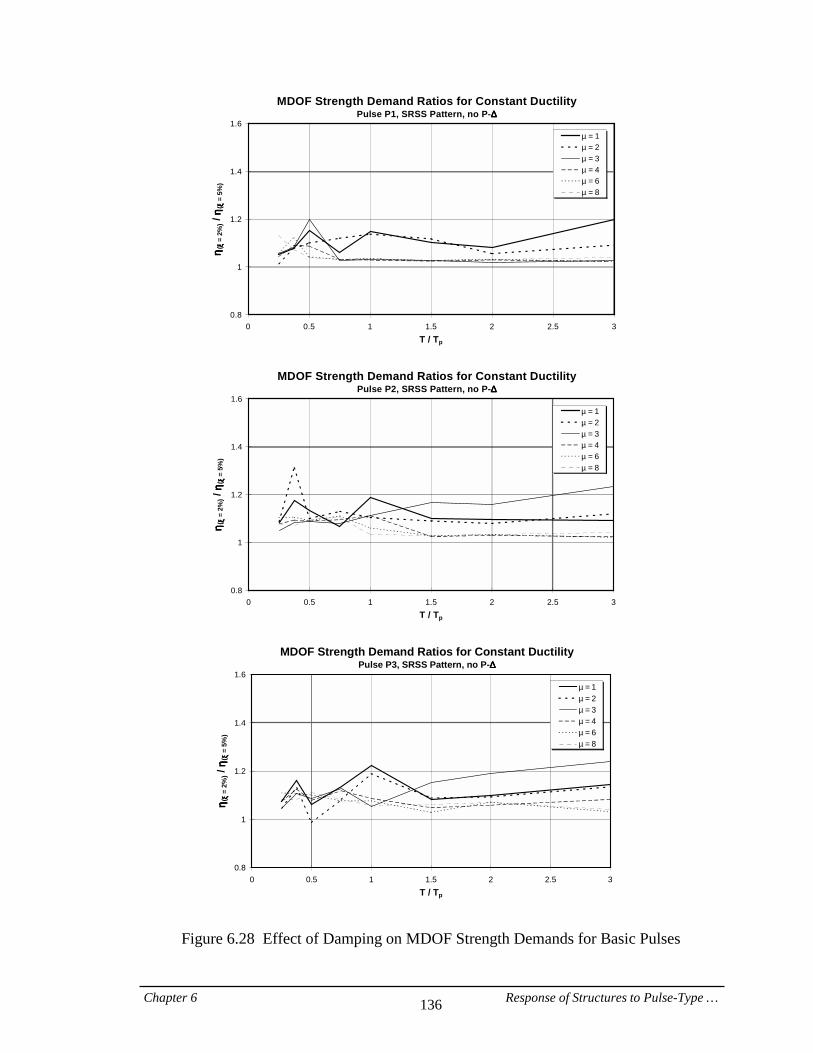
Chapter 6 Response of Structures to Pulse-Type … 136
MDOF Strength Demand Ratios for Constant DuctilityPulse P1, SRSS Pattern, no P-∆∆∆∆
0.8
1
1.2
1.4
1.6
0 0.5 1 1.5 2 2.5 3T / Tp
ηη ηη (ξξ ξξ
= 2%
) / ηη ηη
( ξξ ξξ =
5%
)
µ===1µ===2µ===3µ===4µ===6µ===8
MDOF Strength Demand Ratios for Constant DuctilityPulse P2, SRSS Pattern, no P-∆∆∆∆
0.8
1
1.2
1.4
1.6
0 0.5 1 1.5 2 2.5 3T / Tp
ηη ηη (ξξ ξξ
= 2%
) / ηη ηη
( ξξ ξξ =
5%
)
µ===1µ===2µ===3µ===4µ===6µ===8
MDOF Strength Demand Ratios for Constant DuctilityPulse P3, SRSS Pattern, no P-∆∆∆∆
0.8
1
1.2
1.4
1.6
0 0.5 1 1.5 2 2.5 3T / Tp
ηη ηη (ξξ ξξ
= 2%
) / ηη ηη
( ξξ ξξ =
5%
)
µ===1µ===2µ===3µ===4µ===6µ===8
Figure 6.28 Effect of Damping on MDOF Strength Demands for Basic Pulses

Chapter 6 Response of Structures to Pulse-Type … 137
Normalized Inelastic SDOF Displacement DemandsPulse P1, Bilinear, αααα = 3%, ξξξξ = 2%
0
1
2
3
4
5
0 0.5 1 1.5 2 2.5 3T / Tp
δδ δδ ine
last
ic=
= =
=
// // == == δδ δδel
astic
µ===2
µ===3
µ===4
µ===6
µ===8
Normalized Inelastic SDOF Displacement DemandsPulse P2, Bilinear, αααα = 3%, ξξξξ = 2%
0
1
2
3
4
5
0 0.5 1 1.5 2 2.5 3T / Tp
δδ δδ ine
last
ic=
= =
=
// // == == δδ δδel
astic
µ===2
µ===3
µ===4
µ===6
µ===8
Normalized Inelastic SDOF Displacement DemandsPulse P3, Bilinear, αααα = 3%, ξξξξ = 2%
0
1
2
3
4
5
0 0.5 1 1.5 2 2.5 3T / Tp
δδ δδ ine
last
ic=
= =
=
// // == == δδ δδel
astic
µ===2
µ===3
µ===4
µ===6
µ===8
Figure 6.29 Ratios of Inelastic to Elastic SDOF Displacement Demands for Basic Pulses
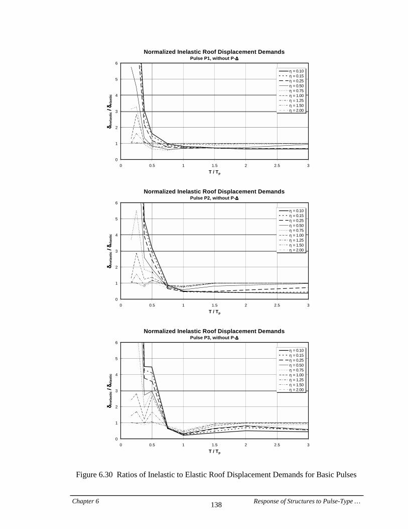
Chapter 6 Response of Structures to Pulse-Type … 138
Normalized Inelastic Roof Displacement DemandsPulse P1, without P-∆∆∆∆
0
1
2
3
4
5
6
0 0.5 1 1.5 2 2.5 3T / Tp
δδ δδ ine
last
ic=
= =
=
// // == == δδ δδel
astic
η===0.10η===0.15η===0.25η===0.50η===0.75η===1.00η===1.25η===1.50η===2.00
Normalized Inelastic Roof Displacement DemandsPulse P2, without P-∆∆∆∆
0
1
2
3
4
5
6
0 0.5 1 1.5 2 2.5 3T / Tp
δδ δδ ine
last
ic=
= =
=
// // == == δδ δδel
astic
η===0.10η===0.15η===0.25η===0.50η===0.75η===1.00η===1.25η===1.50η===2.00
Normalized Inelastic Roof Displacement DemandsPulse P3, without P-∆∆∆∆
0
1
2
3
4
5
6
0 0.5 1 1.5 2 2.5 3T / Tp
δδ δδ ine
last
ic=
= =
=
// // == == δδ δδel
astic
η===0.10η===0.15η===0.25η===0.50η===0.75η===1.00η===1.25η===1.50η===2.00
Figure 6.30 Ratios of Inelastic to Elastic Roof Displacement Demands for Basic Pulses

Chapter 6 Response of Structures to Pulse-Type … 139
SDOF Displacement DemandsPulse P2, Bilinear, αααα = 3%, ξξξξ===== 2%
0
1
2
3
4
0 0.5 1 1.5 2 2.5δδδδmax / ug,max
ηη ηη =
F y /
(m.a
g,m
ax)
T/Tp=0.375
T/Tp=0.50
T/Tp=0.75
T/Tp=1.00
T/Tp=1.50
T/Tp=2.00
T/Tp=3.00
Figure 6.31 Inelastic SDOF Displacement Demands for Pulse P2
Roof Displacement DemandsPulse P2, 20-Story, SRSS Pattern, without P-∆∆∆∆
0
1
2
3
4
0 0.5 1 1.5 2 2.5δδδδroof,max / ug,max
ηη ηη =
V y /
(m.a
g,m
ax)
T/Tp=0.375
T/Tp=0.50
T/Tp=0.75
T/Tp=1.00
T/Tp=1.50
T/Tp=2.00
T/Tp=3.00
Figure 6.32 Inelastic Roof Displacement Demands for Pulse P2
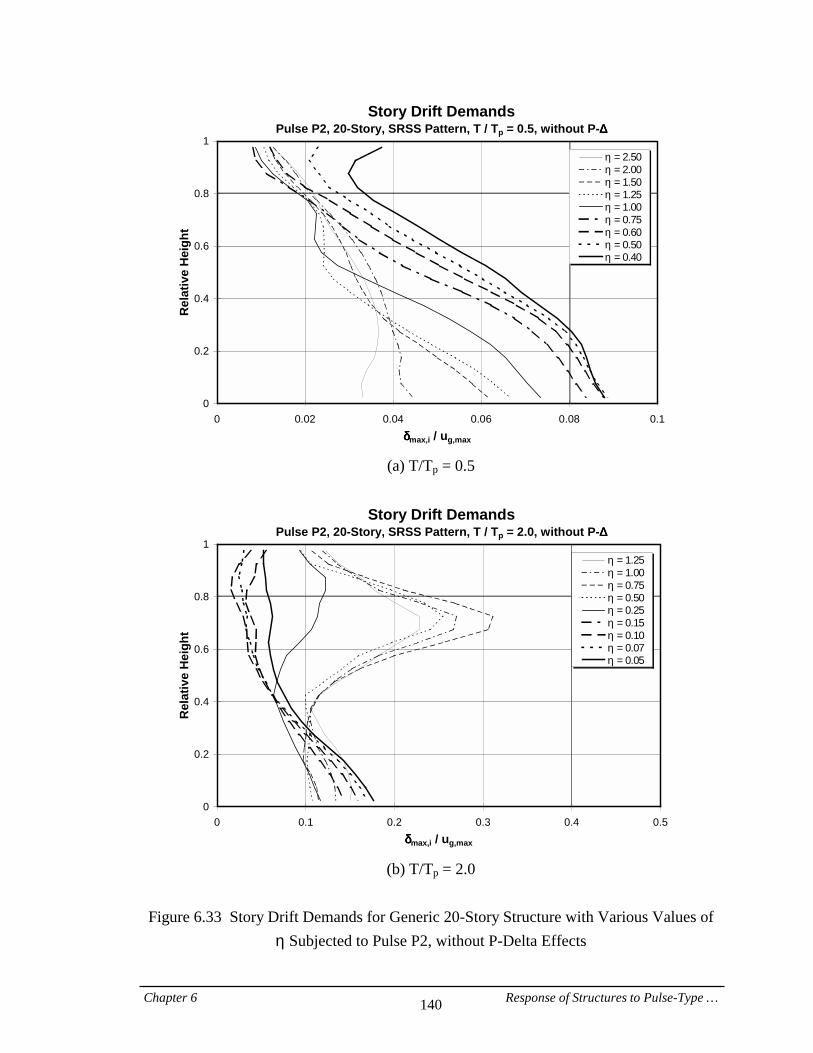
Chapter 6 Response of Structures to Pulse-Type … 140
Story Drift DemandsPulse P2, 20-Story, SRSS Pattern, T / Tp = 0.5, without P-∆∆∆∆
0
0.2
0.4
0.6
0.8
1
0 0.02 0.04 0.06 0.08 0.1δδδδmax,i / ug,max
Rel
ativ
e H
eigh
t
η===2.50η===2.00η===1.50η===1.25η===1.00η===0.75η===0.60η===0.50η===0.40
(a) T/Tp = 0.5
Story Drift Demands
Pulse P2, 20-Story, SRSS Pattern, T / Tp = 2.0, without P-∆∆∆∆
0
0.2
0.4
0.6
0.8
1
0 0.1 0.2 0.3 0.4 0.5δδδδmax,i / ug,max
Rel
ativ
e H
eigh
t
η===1.25η===1.00η===0.75η===0.50η===0.25η===0.15η===0.10η===0.07η===0.05
(b) T/Tp = 2.0
Figure 6.33 Story Drift Demands for Generic 20-Story Structure with Various Values of
η Subjected to Pulse P2, without P-Delta Effects
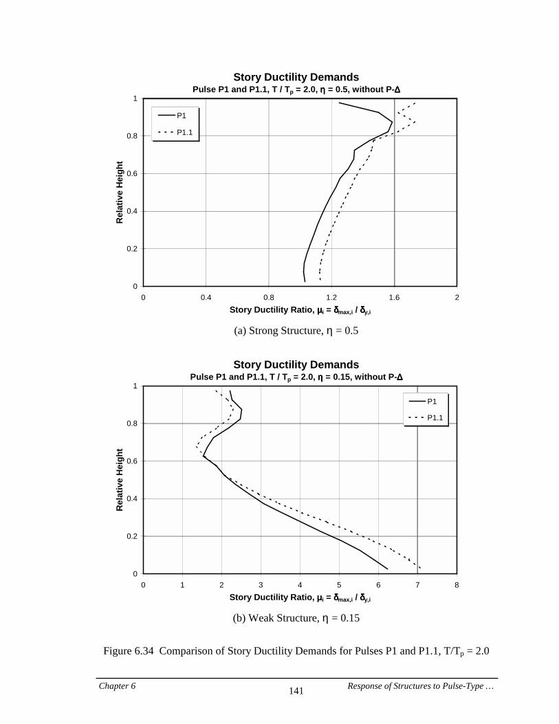
Chapter 6 Response of Structures to Pulse-Type … 141
Story Ductility DemandsPulse P1 and P1.1, T / Tp = 2.0, ηηηη = 0.5, without P-∆∆∆∆
0
0.2
0.4
0.6
0.8
1
0 0.4 0.8 1.2 1.6 2Story Ductility Ratio, µµµµi = δδδδmax,i / δδδδy,i
Rel
ativ
e H
eigh
tP1
P1.1
(a) Strong Structure, η = 0.5
Story Ductility Demands
Pulse P1 and P1.1, T / Tp = 2.0, ηηηη = 0.15, without P-∆∆∆∆
0
0.2
0.4
0.6
0.8
1
0 1 2 3 4 5 6 7 8Story Ductility Ratio, µµµµi = δδδδmax,i / δδδδy,i
Rel
ativ
e H
eigh
t
P1
P1.1
(b) Weak Structure, η = 0.15
Figure 6.34 Comparison of Story Ductility Demands for Pulses P1 and P1.1, T/Tp = 2.0
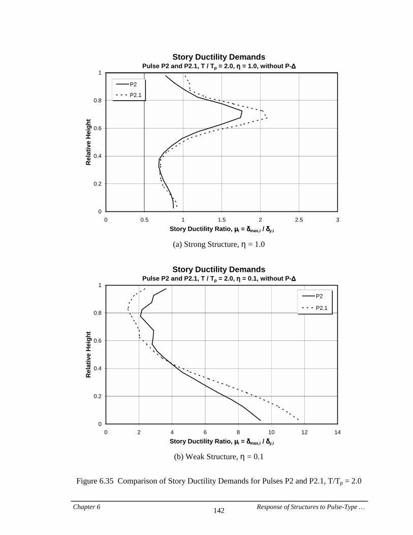
Chapter 6 Response of Structures to Pulse-Type … 142
Story Ductility DemandsPulse P2 and P2.1, T / Tp = 2.0, ηηηη = 1.0, without P-∆∆∆∆
0
0.2
0.4
0.6
0.8
1
0 0.5 1 1.5 2 2.5 3Story Ductility Ratio, µµµµi = δδδδmax,i / δδδδy,i
Rel
ativ
e H
eigh
tP2
P2.1
(a) Strong Structure, η = 1.0
Story Ductility Demands
Pulse P2 and P2.1, T / Tp = 2.0, ηηηη = 0.1, without P-∆∆∆∆
0
0.2
0.4
0.6
0.8
1
0 2 4 6 8 10 12 14Story Ductility Ratio, µµµµi = δδδδmax,i / δδδδy,i
Rel
ativ
e H
eigh
t
P2
P2.1
(b) Weak Structure, η = 0.1
Figure 6.35 Comparison of Story Ductility Demands for Pulses P2 and P2.1, T/Tp = 2.0
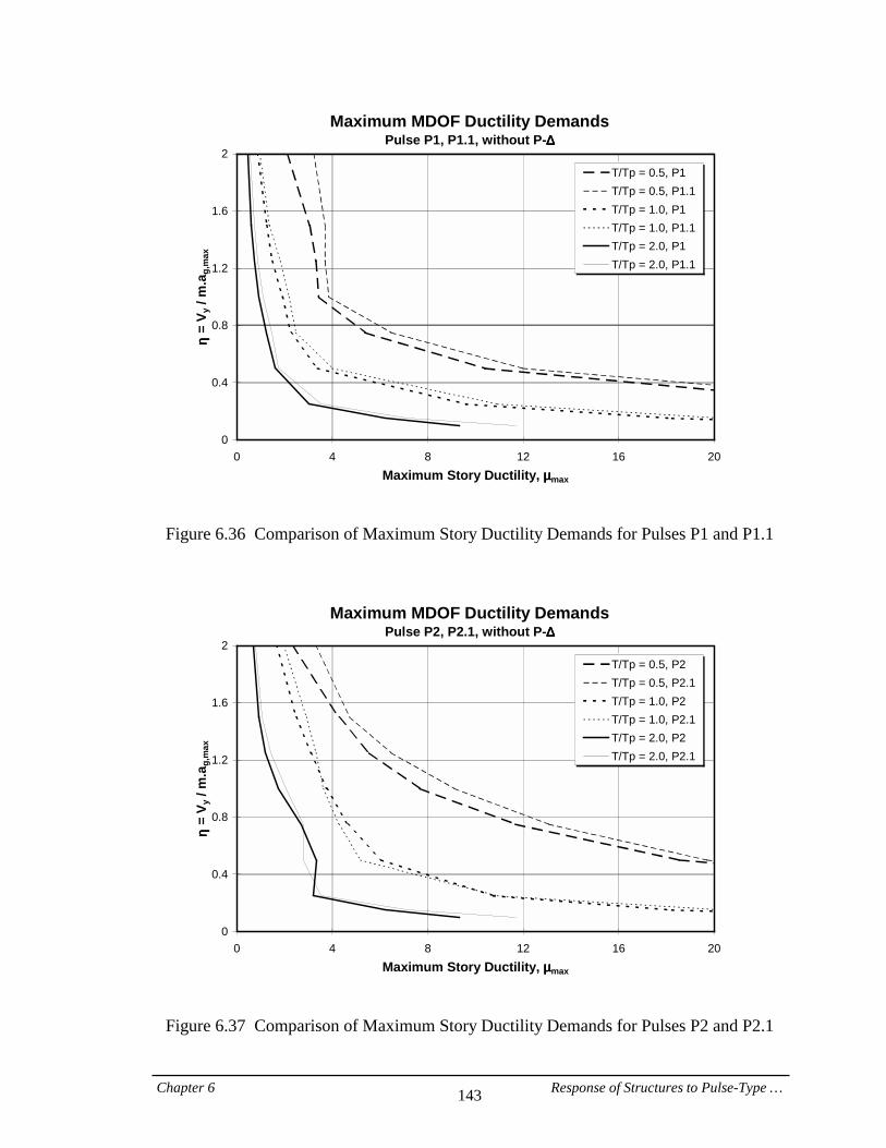
Chapter 6 Response of Structures to Pulse-Type … 143
Maximum MDOF Ductility Demands Pulse P1, P1.1, without P-∆∆∆∆
0
0.4
0.8
1.2
1.6
2
0 4 8 12 16 20Maximum Story Ductility, µµµµmax
ηη ηη =
V y /
m.a
g,m
ax
T/Tp = 0.5, P1T/Tp = 0.5, P1.1T/Tp = 1.0, P1T/Tp = 1.0, P1.1T/Tp = 2.0, P1T/Tp = 2.0, P1.1
Figure 6.36 Comparison of Maximum Story Ductility Demands for Pulses P1 and P1.1
Maximum MDOF Ductility Demands Pulse P2, P2.1, without P-∆∆∆∆
0
0.4
0.8
1.2
1.6
2
0 4 8 12 16 20Maximum Story Ductility, µµµµmax
ηη ηη =
V y /
m.a
g,m
ax
T/Tp = 0.5, P2T/Tp = 0.5, P2.1T/Tp = 1.0, P2T/Tp = 1.0, P2.1T/Tp = 2.0, P2T/Tp = 2.0, P2.1
Figure 6.37 Comparison of Maximum Story Ductility Demands for Pulses P2 and P2.1
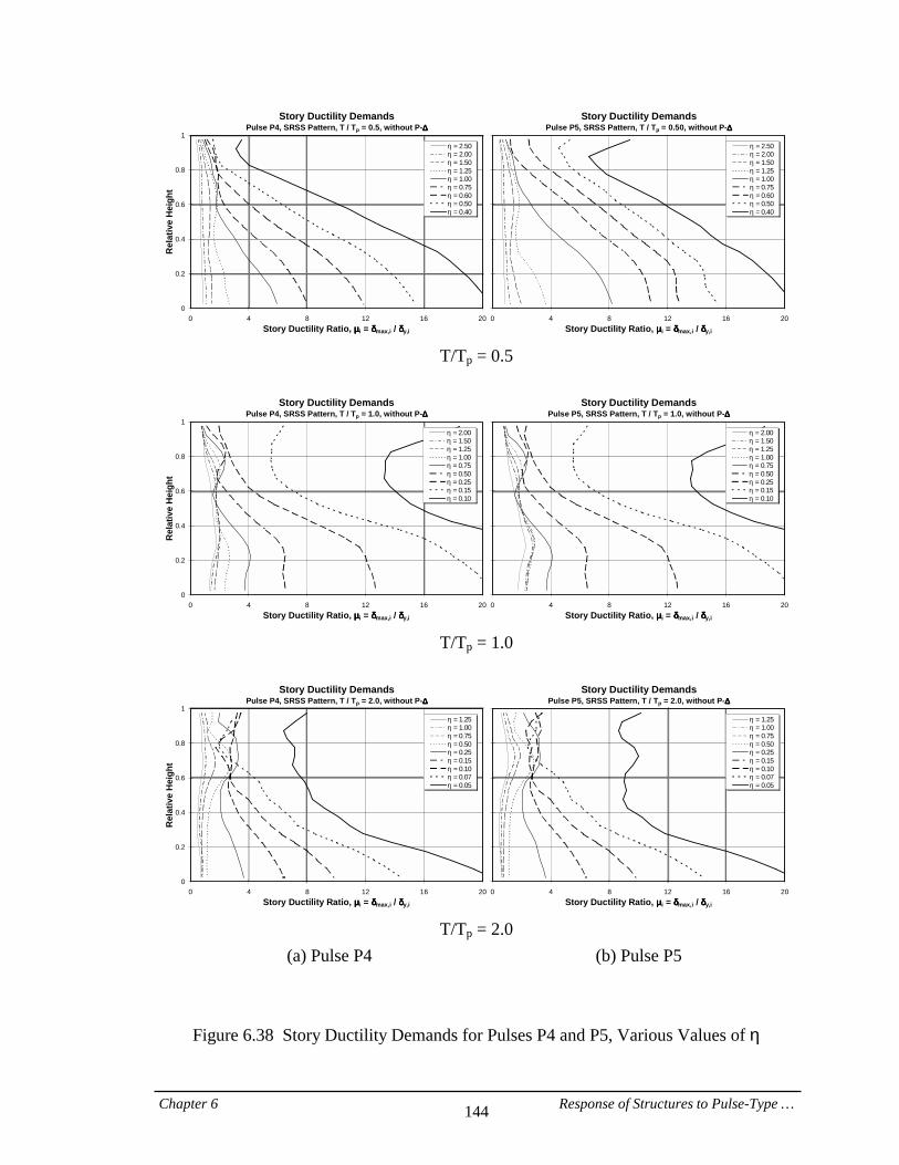
Chapter 6 Response of Structures to Pulse-Type … 144
Story Ductility DemandsPulse P4, SRSS Pattern, T / Tp = 0.5, without P-∆∆∆∆
0
0.2
0.4
0.6
0.8
1
0 4 8 12 16 20Story Ductility Ratio, µµµµi = δδδδmax,i / δδδδy,i
Rel
ativ
e H
eigh
t
η===2.50η===2.00η===1.50η===1.25η===1.00η===0.75η===0.60η===0.50η===0.40
Story Ductility DemandsPulse P5, SRSS Pattern, T / Tp = 0.50, without P-∆∆∆∆
0 4 8 12 16 20Story Ductility Ratio, µµµµi = δδδδmax,i / δδδδy,i
η===2.50η===2.00η===1.50η===1.25η===1.00η===0.75η===0.60η===0.50η===0.40
T/Tp = 0.5
Story Ductility Demands
Pulse P4, SRSS Pattern, T / Tp = 1.0, without P-∆∆∆∆
0
0.2
0.4
0.6
0.8
1
0 4 8 12 16 20Story Ductility Ratio, µµµµi = δδδδmax,i / δδδδy,i
Rel
ativ
e H
eigh
t
η===2.00η===1.50η===1.25η===1.00η===0.75η===0.50η===0.25η===0.15η===0.10
Story Ductility DemandsPulse P5, SRSS Pattern, T / Tp = 1.0, without P-∆∆∆∆
0 4 8 12 16 20Story Ductility Ratio, µµµµi = δδδδmax,i / δδδδy,i
η===2.00η===1.50η===1.25η===1.00η===0.75η===0.50η===0.25η===0.15η===0.10
T/Tp = 1.0
Story Ductility Demands
Pulse P4, SRSS Pattern, T / Tp = 2.0, without P-∆∆∆∆
0
0.2
0.4
0.6
0.8
1
0 4 8 12 16 20Story Ductility Ratio, µµµµi = δδδδmax,i / δδδδy,i
Rel
ativ
e H
eigh
t
η===1.25η===1.00η===0.75η===0.50η===0.25η===0.15η===0.10η===0.07η===0.05
Story Ductility DemandsPulse P5, SRSS Pattern, T / Tp = 2.0, without P-∆∆∆∆
0 4 8 12 16 20Story Ductility Ratio, µµµµi = δδδδmax,i / δδδδy,i
η===1.25η===1.00η===0.75η===0.50η===0.25η===0.15η===0.10η===0.07η===0.05
T/Tp = 2.0
(a) Pulse P4 (b) Pulse P5
Figure 6.38 Story Ductility Demands for Pulses P4 and P5, Various Values of η
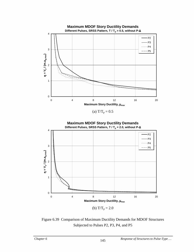
Chapter 6 Response of Structures to Pulse-Type … 145
Maximum MDOF Story Ductility DemandsDifferent Pulses, SRSS Pattern, T / Tp = 0.5, without P-∆∆∆∆
0
1
2
3
4
0 4 8 12 16 20Maximum Story Ductility,,,,====µµµµmax
ηη ηη =
V y /
(m.a
g,m
ax)
P2
P3
P4
P5
=
(a) T/Tp = 0.5 =
Maximum MDOF Story Ductility DemandsDifferent Pulses, SRSS Pattern, T / Tp = 2.0, without P-∆∆∆∆
0
1
2
3
4
0 4 8 12 16 20Maximum Story Ductility,,,,====µµµµmax
ηη ηη =
V y /
(m.a
g,m
ax)
P2
P3
P4
P5
=
(b) T/Tp = 2.0
Figure 6.39 Comparison of Maximum Ductility Demands for MDOF Structures Subjected to Pulses P2, P3, P4, and P5
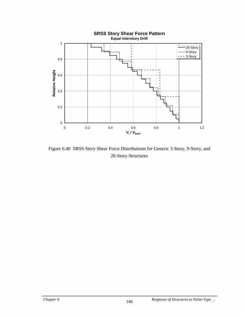
Chapter 6 Response of Structures to Pulse-Type … 146
SRSS Story Shear Force PatternEqual Interstory Drift
0
0.2
0.4
0.6
0.8
1
0 0.2 0.4 0.6 0.8 1 1.2Vi / Vbase
Rel
ativ
e H
eigh
t20-Story9-Story3-Story
Figure 6.40 SRSS Story Shear Force Distributions for Generic 3-Story, 9-Story, and 20-Story Structures
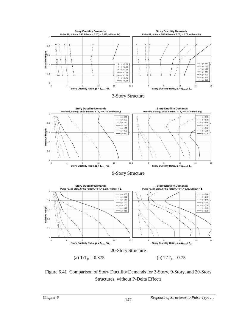
Chapter 6 Response of Structures to Pulse-Type … 147
Story Ductility DemandsPulse P2, 3-Story, SRSS Pattern, T / Tp = 0.375, without P-∆∆∆∆
0
0.2
0.4
0.6
0.8
1
0 4 8 12 16 20Story Ductility Ratio, µµµµi = δδδδmax,i / δδδδy,i
Rel
ativ
e H
eigh
t
η===3.00η===2.00η===1.50η===1.20η===1.00η===0.75η===0.60
Story Ductility DemandsPulse P2, 3-Story, SRSS Pattern, T / Tp = 0.75, without P-∆∆∆∆
0 4 8 12 16 20Story Ductility Ratio, µµµµi = δδδδmax,i / δδδδy,i
η===2.00η===1.25η===1.00η===0.50η===0.30η===0.25η===0.20
3-Story Structure
Story Ductility Demands
Pulse P2, 9-Story, SRSS Pattern, T / Tp = 0.375, without P-∆∆∆∆
0
0.2
0.4
0.6
0.8
1
0 4 8 12 16 20Story Ductility Ratio, µµµµi = δδδδmax,i / δδδδy,i
Rel
ativ
e H
eigh
t
η===3.00η===2.00η===1.50η===1.20η===1.00η===0.75η===0.60
Story Ductility DemandsPulse P2, 9-Story, SRSS Pattern, T / Tp = 0.75, without P-∆∆∆∆
0 4 8 12 16 20Story Ductility Ratio, µµµµi = δδδδmax,i / δδδδy,i
η===2.00η===1.25η===1.00η===0.50η===0.30η===0.25η===0.20
9-Story Structure
Story Ductility Demands
Pulse P2, 20-Story, SRSS Pattern, T / Tp = 0.375, without P-∆∆∆∆
0
0.2
0.4
0.6
0.8
1
0 4 8 12 16 20Story Ductility Ratio, µµµµi = δδδδmax,i / δδδδy,i
Rel
ativ
e H
eigh
t
η===3.00η===2.00η===1.50η===1.20η===1.00η===0.75η===0.60
Story Ductility DemandsPulse P2, 20-Story, SRSS Pattern, T / Tp = 0.75, without P-∆∆∆∆
0 4 8 12 16 20Story Ductility Ratio, µµµµi = δδδδmax,i / δδδδy,i
η===2.00η===1.25η===1.00η===0.50η===0.30η===0.25η===0.20
20-Story Structure
(a) T/Tp = 0.375 (b) T/Tp = 0.75
Figure 6.41 Comparison of Story Ductility Demands for 3-Story, 9-Story, and 20-Story Structures, without P-Delta Effects

Chapter 6 Response of Structures to Pulse-Type … 148
Story Ductility DemandsPulse P2, 3-Story, SRSS Pattern, T / Tp = 1.0, without P-∆∆∆∆
0
0.2
0.4
0.6
0.8
1
0 4 8 12 16 20Story Ductility Ratio, µµµµi = δδδδmax,i / δδδδy,i
Rel
ativ
e H
eigh
t
η===2.00η===1.50η===1.00η===0.50η===0.25η===0.15η===0.10
Story Ductility DemandsPulse P2, 3-Story, SRSS Pattern, T / Tp = 2.0, without P-∆∆∆∆
0 4 8 12 16 20Story Ductility Ratio, µµµµi = δδδδmax,i / δδδδy,i
η===1.00η===0.75η===0.50η===0.25η===0.10η===0.07η===0.05
3-Story Structure
Story Ductility Demands
Pulse P2, 9-Story, SRSS Pattern, T / Tp = 1.0, without P-∆∆∆∆
0
0.2
0.4
0.6
0.8
1
0 4 8 12 16 20Story Ductility Ratio, µµµµi = δδδδmax,i / δδδδy,i
Rel
ativ
e H
eigh
t
η===2.00η===1.50η===1.00η===0.50η===0.25η===0.15η===0.10
Story Ductility DemandsPulse P2, 9-Story, SRSS Pattern, T / Tp = 2.0, without P-∆∆∆∆
0 4 8 12 16 20Story Ductility Ratio, µµµµi = δδδδmax,i / δδδδy,i
η===1.00η===0.75η===0.50η===0.25η===0.10η===0.07η===0.05
9-Story Structure
Story Ductility Demands
Pulse P2, 20-Story, SRSS Pattern, T / Tp = 1.0, without P-∆∆∆∆
0
0.2
0.4
0.6
0.8
1
0 4 8 12 16 20Story Ductility Ratio, µµµµi = δδδδmax,i / δδδδy,i
Rel
ativ
e H
eigh
t
η===2.00η===1.50η===1.00η===0.50η===0.25η===0.15η===0.10
Story Ductility DemandsPulse P2, 20-Story, SRSS Pattern, T / Tp = 2.0, without P-∆∆∆∆
0 4 8 12 16 20Story Ductility Ratio, µµµµi = δδδδmax,i / δδδδy,i
η===1.00η===0.75η===0.50η===0.25η===0.10η===0.07η===0.05
20-Story Structure
(c) T/Tp = 1.0 (d) T/Tp = 2.0
Figure 6.41 (Cont’d) Comparison of Story Ductility Demands for 3-Story, 9-Story, and 20-Story Structures, without P-Delta Effects
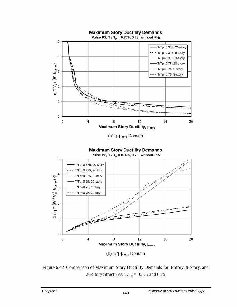
Chapter 6 Response of Structures to Pulse-Type … 149
Maximum Story Ductility DemandsPulse P2, T / Tp = 0.375, 0.75, without P-∆∆∆∆
0
1
2
3
4
5
0 4 8 12 16 20Maximum Story Ductility,,,,====µµµµmax
ηη ηη =
V y /
(m.a
g,m
ax)
T/Tp=0.375, 20-story
T/Tp=0.375, 9-story
T/Tp=0.375, 3-story
T/Tp=0.75, 20-story
T/Tp=0.75, 9-story
T/Tp=0.75, 3-story
(a) η-µmax Domain
Maximum Story Ductility Demands
Pulse P2, T / Tp = 0.375, 0.75, without P-∆∆∆∆
0
1
2
3
4
5
0 4 8 12 16 20Maximum Story Ductility,,,,====µµµµmax
1 / ηη ηη
= (W
/ V y
) ag,
max
/ g
T/Tp=0.375, 20-story
T/Tp=0.375, 9-story
T/Tp=0.375, 3-story
T/Tp=0.75, 20-story
T/Tp=0.75, 9-story
T/Tp=0.75, 3-story
(b) 1/η-µmax Domain
Figure 6.42 Comparison of Maximum Story Ductility Demands for 3-Story, 9-Story, and
20-Story Structures, T/Tp = 0.375 and 0.75
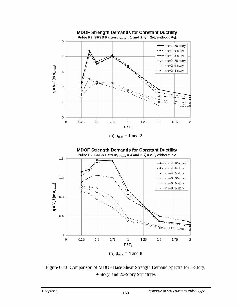
Chapter 6 Response of Structures to Pulse-Type … 150
MDOF Strength Demands for Constant DuctilityPulse P2, SRSS Pattern, µµµµmax = 1 and 2, ξξξξ = 2%, without P-∆∆∆∆
0
1
2
3
4
5
0 0.25 0.5 0.75 1 1.25 1.5 1.75 2
T / Tp
ηη ηη =
V y /
(m.a
g,m
ax)
mu=1, 20-storymu=1, 9-storymu=1, 3-storymu=2, 20-storymu=2, 9-storymu=2, 3-story
(a) µmax = 1 and 2
MDOF Strength Demands for Constant DuctilityPulse P2, SRSS Pattern, µµµµmax = 4 and 8, ξξξξ = 2%, without P-∆∆∆∆
0
0.4
0.8
1.2
1.6
0 0.25 0.5 0.75 1 1.25 1.5 1.75 2T / Tp
ηη ηη =
V y /
(m.a
g,m
ax)
mu=4, 20-storymu=4, 9-storymu=4, 3-storymu=8, 20-storymu=8, 9-storymu=8, 3-story
(b) µmax = 4 and 8
Figure 6.43 Comparison of MDOF Base Shear Strength Demand Spectra for 3-Story,
9-Story, and 20-Story Structures
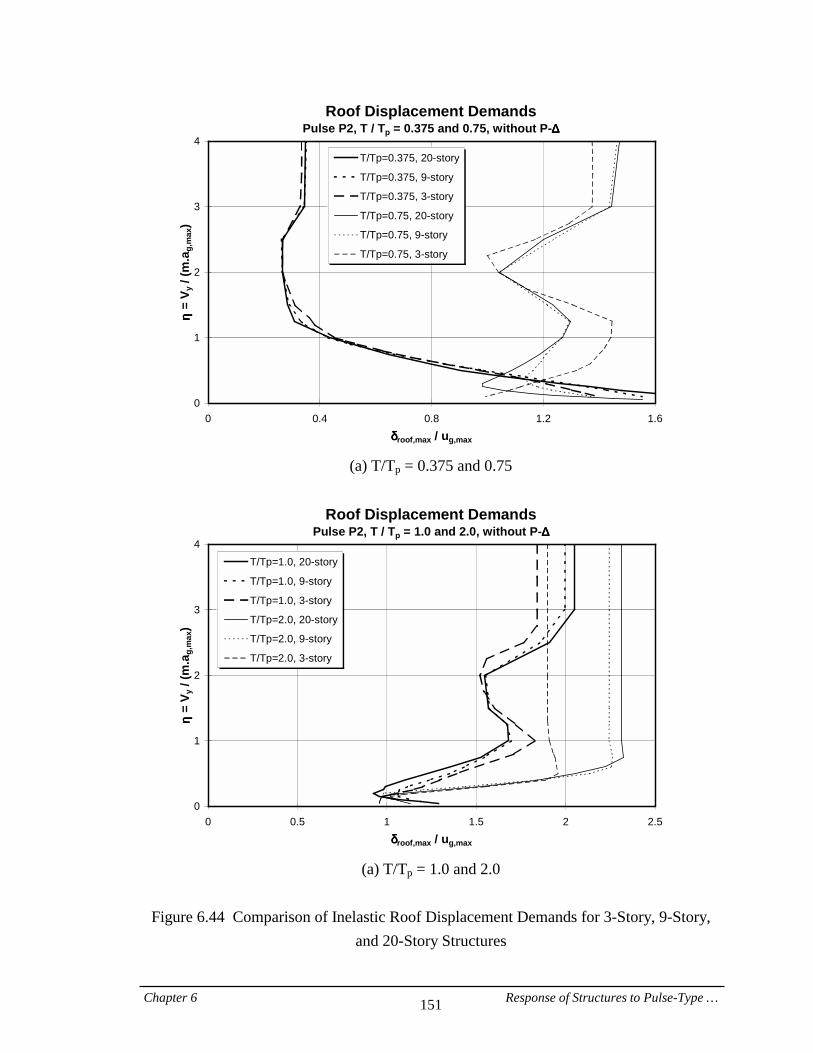
Chapter 6 Response of Structures to Pulse-Type … 151
Roof Displacement DemandsPulse P2, T / Tp = 0.375 and 0.75, without P-∆∆∆∆
0
1
2
3
4
0 0.4 0.8 1.2 1.6δδδδroof,max / ug,max
ηη ηη =
V y /
(m.a
g,m
ax)
T/Tp=0.375, 20-story
T/Tp=0.375, 9-story
T/Tp=0.375, 3-story
T/Tp=0.75, 20-story
T/Tp=0.75, 9-story
T/Tp=0.75, 3-story
(a) T/Tp = 0.375 and 0.75
Roof Displacement Demands
Pulse P2, T / Tp = 1.0 and 2.0, without P-∆∆∆∆
0
1
2
3
4
0 0.5 1 1.5 2 2.5δδδδroof,max / ug,max
ηη ηη =
V y /
(m.a
g,m
ax)
T/Tp=1.0, 20-story
T/Tp=1.0, 9-story
T/Tp=1.0, 3-story
T/Tp=2.0, 20-story
T/Tp=2.0, 9-story
T/Tp=2.0, 3-story
(a) T/Tp = 1.0 and 2.0
Figure 6.44 Comparison of Inelastic Roof Displacement Demands for 3-Story, 9-Story,
and 20-Story Structures
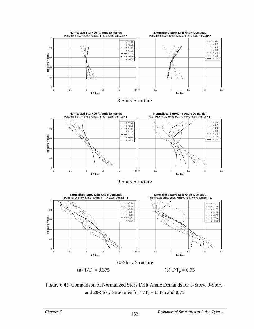
Chapter 6 Response of Structures to Pulse-Type … 152
Normalized Story Drift Angle DemandsPulse P2, 3-Story, SRSS Pattern, T / Tp = 0.375, without P-∆∆∆∆
0
0.2
0.4
0.6
0.8
1
0 0.5 1 1.5 2 2.5θθθθi / θθθθroof
Rel
ativ
e H
eigh
t
η===3.00η===2.00η===1.50η===1.20η===1.00η===0.75η===0.60
Normalized Story Drift Angle DemandsPulse P2, 3-Story, SRSS Pattern, T / Tp = 0.75, without P-∆∆∆∆
0 0.5 1 1.5 2 2.5θθθθi / θθθθroof
η===2.00η===1.25η===1.00η===0.50η===0.30η===0.25η===0.20
3-Story Structure
Normalized Story Drift Angle Demands
Pulse P2, 9-Story, SRSS Pattern, T / Tp = 0.375, without P-∆∆∆∆
0
0.2
0.4
0.6
0.8
1
0 0.5 1 1.5 2 2.5θθθθi / θθθθroof
Rel
ativ
e H
eigh
t
η===3.00η===2.00η===1.50η===1.20η===1.00η===0.75η===0.60
Normalized Story Drift Angle DemandsPulse P2, 9-Story, SRSS Pattern, T / Tp = 0.75, without P-∆∆∆∆
0 0.5 1 1.5 2 2.5θθθθi / θθθθroof
η===2.00η===1.25η===1.00η===0.50η===0.30η===0.25η===0.20
9-Story Structure
Normalized Story Drift Angle Demands
Pulse P2, 20-Story, SRSS Pattern, T / Tp = 0.375, without P-∆∆∆∆
0
0.2
0.4
0.6
0.8
1
0 0.5 1 1.5 2 2.5θθθθi / θθθθroof
Rel
ativ
e H
eigh
t
η===3.00η===2.00η===1.50η===1.20η===1.00η===0.75η===0.60
Normalized Story Drift Angle DemandsPulse P2, 20-Story, SRSS Pattern, T / Tp = 0.75, without P-∆∆∆∆
0 0.5 1 1.5 2 2.5θθθθi / θθθθroof
η===2.00η===1.25η===1.00η===0.50η===0.30η===0.25η===0.20
20-Story Structure
(a) T/Tp = 0.375 (b) T/Tp = 0.75
Figure 6.45 Comparison of Normalized Story Drift Angle Demands for 3-Story, 9-Story, and 20-Story Structures for T/Tp = 0.375 and 0.75
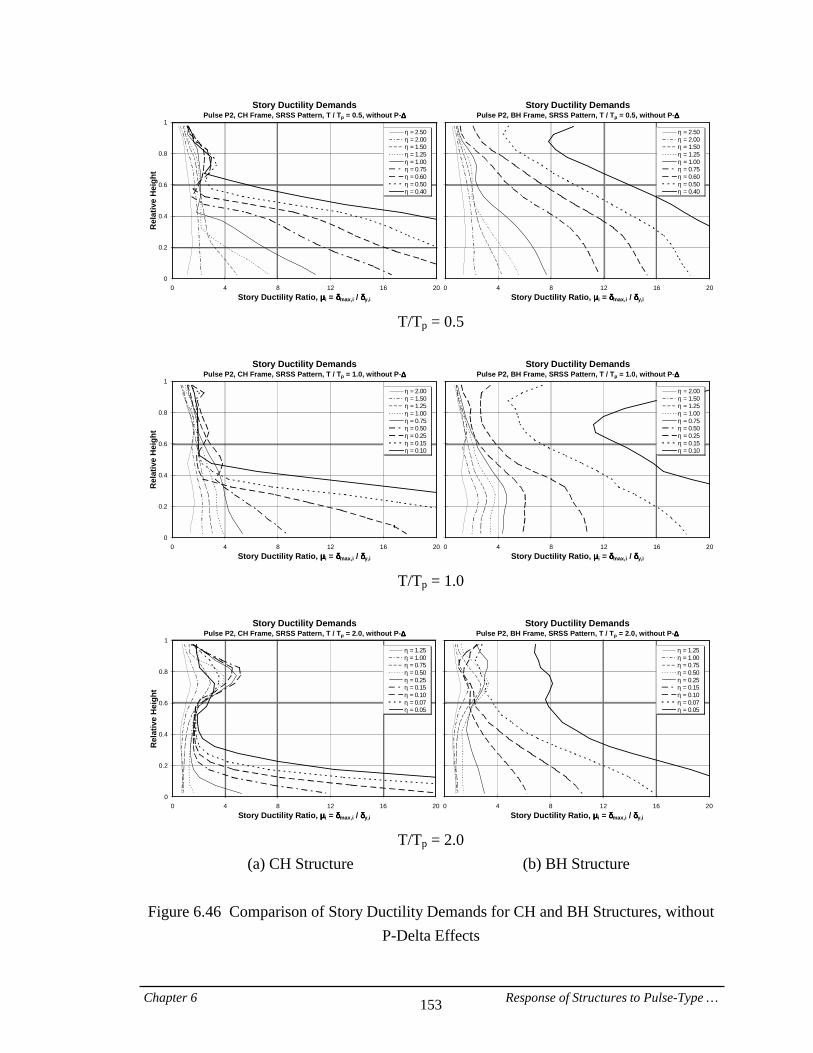
Chapter 6 Response of Structures to Pulse-Type … 153
Story Ductility DemandsPulse P2, CH Frame, SRSS Pattern, T / Tp = 0.5, without P-∆∆∆∆
0
0.2
0.4
0.6
0.8
1
0 4 8 12 16 20Story Ductility Ratio, µµµµi = δδδδmax,i / δδδδy,i
Rel
ativ
e H
eigh
t
η===2.50η===2.00η===1.50η===1.25η===1.00η===0.75η===0.60η===0.50η===0.40
Story Ductility DemandsPulse P2, BH Frame, SRSS Pattern, T / Tp = 0.5, without P-∆∆∆∆
0 4 8 12 16 20Story Ductility Ratio, µµµµi = δδδδmax,i / δδδδy,i
η===2.50η===2.00η===1.50η===1.25η===1.00η===0.75η===0.60η===0.50η===0.40
T/Tp = 0.5
Story Ductility Demands
Pulse P2, CH Frame, SRSS Pattern, T / Tp = 1.0, without P-∆∆∆∆
0
0.2
0.4
0.6
0.8
1
0 4 8 12 16 20Story Ductility Ratio, µµµµi = δδδδmax,i / δδδδy,i
Rel
ativ
e H
eigh
t
η===2.00η===1.50η===1.25η===1.00η===0.75η===0.50η===0.25η===0.15η===0.10
Story Ductility DemandsPulse P2, BH Frame, SRSS Pattern, T / Tp = 1.0, without P-∆∆∆∆
0 4 8 12 16 20Story Ductility Ratio, µµµµi = δδδδmax,i / δδδδy,i
η===2.00η===1.50η===1.25η===1.00η===0.75η===0.50η===0.25η===0.15η===0.10
T/Tp = 1.0
Story Ductility Demands
Pulse P2, CH Frame, SRSS Pattern, T / Tp = 2.0, without P-∆∆∆∆
0
0.2
0.4
0.6
0.8
1
0 4 8 12 16 20Story Ductility Ratio, µµµµi = δδδδmax,i / δδδδy,i
Rel
ativ
e H
eigh
t
η===1.25η===1.00η===0.75η===0.50η===0.25η===0.15η===0.10η===0.07η===0.05
Story Ductility DemandsPulse P2, BH Frame, SRSS Pattern, T / Tp = 2.0, without P-∆∆∆∆
0 4 8 12 16 20Story Ductility Ratio, µµµµi = δδδδmax,i / δδδδy,i
η===1.25η===1.00η===0.75η===0.50η===0.25η===0.15η===0.10η===0.07η===0.05
T/Tp = 2.0
(a) CH Structure (b) BH Structure
Figure 6.46 Comparison of Story Ductility Demands for CH and BH Structures, without P-Delta Effects
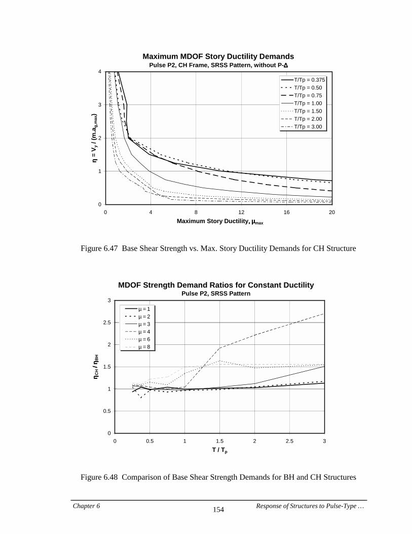
Chapter 6 Response of Structures to Pulse-Type … 154
Maximum MDOF Story Ductility DemandsPulse P2, CH Frame, SRSS Pattern, without P-∆∆∆∆
0
1
2
3
4
0 4 8 12 16 20Maximum Story Ductility,,,,====µµµµmax
ηη ηη =
V y /
(m.a
g,m
ax)
T/Tp = 0.375T/Tp = 0.50T/Tp = 0.75T/Tp = 1.00T/Tp = 1.50T/Tp = 2.00T/Tp = 3.00
Figure 6.47 Base Shear Strength vs. Max. Story Ductility Demands for CH Structure
MDOF Strength Demand Ratios for Constant DuctilityPulse P2, SRSS Pattern
0
0.5
1
1.5
2
2.5
3
0 0.5 1 1.5 2 2.5 3T / Tp
ηη ηη CH== ==
// // == == ηη ηηB
H
µ===1µ===2µ===3µ===4µ===6µ===8
Figure 6.48 Comparison of Base Shear Strength Demands for BH and CH Structures
Chapter 7 Representation of Near-Fault Ground … 155
CHAPTER 7
REPRESENTATION OF NEAR-FAULT GROUND MOTIONS BY EQUIVALENT PULSES
In Chapters 2 and 4 it was shown that near-fault ground motions come in large variations. This variety very much complicates the evaluation or prediction of structural response unless near-fault ground motions can be represented by a small number of simplified motions that can reasonably replicate important near-fault response characteristics. An inspection of the time history records (especially velocity and displacement) of near-fault ground motions reveals their impulsive characteristics (see Appendix A). The study of similarities between the response of structures subjected to near-fault records and simple pulses also provides much evidence that, within limitations, near-fault records can be represented by equivalent pulses of the type introduced in Chapter 5. However, it is not reasonable to expect that perfect equivalence can be established between near-fault ground motions and simple pulses for the full range of interest. Near-fault records usually contain high frequency components that have little to do with the characteristics of the long-period high-energy pulse generated by the propagation of fault rupture. As will be shown in this chapter, in the very short period range these high frequency contents make the pulse-record equivalence questionable. Furthermore, in the very long period range it is also likely that other phenomena (e.g., basin effects or instrument limitations) contaminate the record. This chapter presents procedures that can be used to identify the parameters of the predominant pulse contained in near-fault ground motions. Using these procedures, equivalent pulses are established for the fault-normal component of the records with forward directivity introduced in Chapter 2. Then, the capability of the equivalent pulses to replicate the salient SDOF and MDOF response attributes of near-fault ground motions
Chapter 7 Representation of Near-Fault Ground … 156
is evaluated. Finally, equivalent pulses are established and evaluated for the rotated components of the near-fault records. 7.1. Matching of Near-Fault Ground Motions to Equivalent Pulses It is necessary to estimate the period range in which simple pulses can represent near-fault records with reasonable confidence. As shown in Fig. 5.4, the elastic strength demand (acceleration) spectra of the basic pulses demonstrate a relatively deep valley at T/Tp = 0.25, where T is the fundamental period of the structure and Tp is the period of the pulse. The valley, however, disappears in the inelastic strength spectra on account of post-yield period elongation, and even turns into a wide peak at very large ductilities. Furthermore, there are a number of close peaks and valleys in the elastic spectrum of the simple pulses in the period range of T/Tp < 0.25. These observations are incompatible with the spectra of recorded near-fault ground motions (see Appendix A), indicating questionable equivalence between near-fault records and simple pulses in the very short period range, i.e., T/Tp ≤ 0.25. Hence, it is postulated that the equivalence between a near-fault record and a basic pulse can be reasonably established within the range of T/Tp from 0.375 to 3.0. Even though much effort has been devoted to establishing such equivalence through a systematic procedure, it cannot be claimed that the outcome of this procedure is an equivalent pulse that can perfectly represent the near-fault ground motion. For many of the records used in this study an equivalent pulse has been successfully established, but not all near-fault records have become part of this success. It is important to note that the use of equivalent pulses is an approximation to a very complex problem. If this approximation proves to be reasonably effective, it can significantly simplify the process of predicting near-fault demands. The extent of this approximation is evaluated in Section 7.2. 7.1.1. Parameters of Equivalent Pulses The basic pulses introduced in Chapter 5, i.e., P1, P2, and P3 are utilized here as equivalent pulses for near-fault ground motions. It was shown that the other pulse motions (triangular pulses and pulses with different duration) are adequately represented by the three basic pulses for practical purposes. In order to establish an equivalent pulse for a record, three parameters need to be evaluated; pulse type (P1, P2, or P3), pulse
Chapter 7 Representation of Near-Fault Ground … 157
period Tp, and pulse intensity. The peak ground acceleration of the square wave history, ag,max, is used for the latter purpose (see Figs. 5.1 to 5.3). These three parameters completely characterize the equivalent pulse, and therefore its time history and response properties can be derived accordingly. In the following discussion the ag,max and vg,max of the equivalent pulse are referred to as the effective acceleration, aeff, and the effective velocity, veff, respectively. The equivalent pulse intensity can also be quantified by the (effective) peak velocity because the pulse peak acceleration and velocity are related, i.e., veff = aeffTp/4. As shown in the following section, the effective velocity is a more convenient pulse intensity measure since it is usually close to the recorded peak ground velocity of the ground motion. Nevertheless, the effective acceleration is more useful for design purposes due to its direct relationship with the structure strength coefficient η = Vy/(m.aeff). 7.1.2. Procedure for Matching In this study the equivalent pulse parameters are estimated using engineering rather than seismological considerations. As pointed out before, the equivalent pulse is by no means a precise representation for near-fault ground motions. In many cases, inspection, common sense, and judgmental decisions need to be employed in order to arrive at a final value for the equivalent pulse parameters. Some of these decisions are validated using a sensitivity analysis. Pulse Type and Pulse Period: Mostly judgment is employed to decide on the pulse type, based on an inspection of the time history trace, and on a comparison between ground motion and pulse spectral shapes (primarily velocity and displacement spectra). An inspection of the ground displacement and velocity time histories of the records (fault-normal component) investigated in this research reveals that none of the near-fault ground motions exhibits motions of the type represented by pulse P1, which has a half velocity cycle with a permanent ground displacement. Therefore, only equivalent pulses of type P2 (full cycle) and P3 (multi-cycle) are employed to represent the records. Since the velocity response spectra of basic pulses P2 and P3 show a clear hump at T/Tp = 1 (see Fig. 5.4), the pulse period Tp for a near-fault record is identified from the
Chapter 7 Representation of Near-Fault Ground … 158
location of a global and clear peak in the velocity response spectrum. Typical examples are illustrated in Figs. 7.1 to 7.3, which show the velocity and displacement spectra of the three basic pulses superimposed on the velocity and displacement spectra of near-fault records NR94rrs, KB95kobj, and KB95tato. In these figures the pulse and ground motion spectra are compared in a normalized domain. The period of the structure is normalized by the pulse period and the spectral ordinates are normalized by corresponding time history peak values. In most cases a narrow range for Tp could be identified rigorously. But in some other cases, in which the peak is not clear or there are two or more peaks (e.g., Fig. 7.3), judgment has to be employed to decide on a final value. A sensitivity analysis is performed in Section 7.2.3 to evaluate these decisions. Pulse Intensity: Various procedures were investigated to determine the effective pulse acceleration aeff; the simplest one being the estimation of aeff from the elastic displacement spectra (equating pulse and ground motion spectral displacement at T = Tp). However, inconsistent results were obtained when the so estimated values were used to compute ductility demands for MDOF systems. The reason is that when aeff is determined based on elastic spectra only, no consideration is given to inelastic MDOF response characteristics. Ultimately, a rigorous process is employed whose objective is to minimize the differences between the maximum story ductility demands obtained from the near-fault ground motion and the equivalent pulse. In summary the procedure includes the following steps:
1. Compute the η−µmax curves for the appropriate pulse type for T/Tp = 0.375, 0.5, 0.75, 1.0, 1.5, 2.0, and 3.0.
2. Compute the γ−µmax curves for the near-fault record for T/Tp = 0.375, 0.5, 0.75, 1.0, 1.5, 2.0, and 3.0.
3. For each T/Tp value, convert the η-µmax curve of the pulse into a γ−µmax curve [γ = Vy/(m.g) = (aeff/g)η] and find best-fit values for aeff by minimizing the relative differences between the two γ−µmax curves. The minimization technique is explained in more detail next.
4. Obtain final values for aeff by averaging the best-fit values for the seven period ratios.

Chapter 7 Representation of Near-Fault Ground … 159
The relative difference between the γ−µmax curves of the pulse and near-fault record at a given ductility value of µi is defined as:
Ei
Pi
effEi
Pi
Ei
Pi
Ei
i )g/a(11eγη−=
γγ−=
γ
γ−γ= (7.1)
where γi
E and γiP represent the strength coefficients corresponding to the ground motion
and the pulse, respectively, at µi. The difference (error) values ei are calculated for discrete ductility ratios in the range of interest. Then, using the least-squares method, the best-fit value for aeff is evaluated such that the differences between the two curves are minimized, i.e., Σ(ei)2 is minimum. But, minimizing the sum of the squared errors is the same as minimizing the mean of the squared errors, which is equal to: Mean[(ei)2] = Var[ei] + (Mean[ei])2 = (Mean[ei])2(1+Ve
2) (7.2) where Var[ei] is the variance of the error and Ve represents the coefficient of variation of the error in the range in which the difference between the two curves is minimized. This is again equivalent to minimizing the square root of the quantity shown in Eq. 7.2, which can be written as:
2ei
2i V1])e[Mean(])e[(Mean += (7.3)
This shows that by using the least-squares method, the quantity given by Eq. 7.3, which is a combination of the mean error and the error dispersion, is minimized. This quantity can be used as a good measure to assess the final proximity of the two γ-µmax curves resulting from the error minimization procedure. Smaller values for this quantity imply a closer match between the two curves. Through the procedure described above, values for aeff can be obtained that minimize the differences between the γ-µmax curves corresponding to the pulse and record in a given range of ductility, µmax. In this study the following ranges of µmax are investigated:
• = µmax = 1 to 10, which covers the full range of interest. • = µmax = 4 to 10, which represents behavior at a low performance level. • = µmax = 1.0, which represents behavior at a high performance level.
Chapter 7 Representation of Near-Fault Ground … 160
The results of this procedure for the fault-normal component of the recorded near-fault ground motions introduced in Chapter 2 are presented in Table 7.1. For each ductility range and T/Tp ratio, the best-fit value for aeff is shown as well as the quantity given by Eq. 7.3, the mean error, and the error coefficient of variation. The results are tabulated only for the near-fault records with forward directivity. The Landers (Lucerne) record (LN92lucr) is omitted from Table 7.1 because it has a pulse period longer than 4 seconds (see the velocity spectrum in Fig. A.2), which may be contaminated by instrument errors. Besides, the matching procedure for this record would require computing the demands for structures with unreasonably long periods (e.g., T = 3Tp > 12.0 sec.). As explained in the last step of the procedure, the final value for aeff is arrived at by averaging the best-fit values for the seven period ratios. Figure 7.4 illustrates the variations of the aeff values obtained for the recorded ground motions using different T/Tp values and the full period range of interest (1 to 10). For each record the aeff values are normalized by their average. To make the picture more readable, the results are presented in two separate graphs, each corresponding to 7 near-fault records. As can be seen, the aeff values obtained from the matching procedure are not very sensitive to T/Tp. This justifies averaging the values in order to arrive at a single pulse intensity measure for a given near-fault ground motion. The results presented in Table 7.1 are summarized in Table 7.2 by averaging the aeff values obtained for various T/Tp ratios for the recorded ground motions. The table lists pulse type and period, as well as effective acceleration and peak velocity of the equivalent pulse for the three ductility ranges. As expected, the values of aeff differ somewhat but not by a large amount among the three ductility ranges. Having estimates of Tp and aeff, the peak velocity of the pulse can be computed (veff = aeffTp/4). Comparing the so computed veff with the peak ground velocity PGV listed in the last column of Table 7.2 indicates that in most of the cases the peak velocity of the equivalent pulse is within 20% of the PGV of the near-fault record. Thus, it appears to be feasible to use the peak ground velocity of the near-fault record, PGV, to estimate the pulse intensity parameter (i.e., aeff = 4PGV/Tp) rather than employing the complex procedure outlined here. A summary of the results for the fault-normal component of the simulated ground motions with forward directivity (see Chapter 2), derived in the same manner as for the recorded ground motions, is listed in Table 7.3. Again, the results indicate that in most of

Chapter 7 Representation of Near-Fault Ground … 161
the cases the peak velocity of the equivalent pulse is very close to the peak ground velocity (PGV) of the ground motion record. 7.2. Evaluation of Equivalent Pulses In the previous section the parameters of equivalent pulses were identified for the near-fault records investigated in this study. An important issue that needs to be addressed is to what extent this representation is reasonable, practical, and reliable. It should be considered that simple pulse representation of complex near-fault records is not expected to be precise because near-fault ground motions are affected by many complex seismological phenomena. The objective is not to develop pulses that can accurately replicate recorded ground motions, but to develop pulses that can reasonably simulate predominant response characteristics of structures located in the near-fault region of a seismic source. In this section demands for structures subjected to near-fault records are compared to the corresponding demands obtained from the equivalent pulses of those records. The equivalent pulse parameters identified for the ductility range from 1 to 10 are utilized for this purpose. The main goal is to evaluate the quality of the pulse-record equivalence established previously. 7.2.1. Comparison of SDOF Response Time Histories In this section elastic and inelastic responses of SDOF systems subjected to the near-fault record NR94rrs are compared qualitatively with the corresponding responses for Pulse P2. As listed in Table 7.2, the near-fault record NR94rrs has an equivalent pulse of type P2 with a period of Tp = 1.0 sec. Figure 7.5 illustrates the inelastic displacement response time history normalized by the maximum ground displacement for Pulse P2 and T/Tp ratios of 1.0 and 2.0. Each graph represents the ground displacement time history (denoted as “Ugr”) together with the displacement response time history (denoted as “Ust”) of a system with a ductility of µ = 6. Figure 7.6 shows the ground and response time histories for the near-fault record NR94rrs in a similar manner. The following observations can be made:
• = The ground displacement time history of NR94rrs looks different from the time history of P2, with the greatest difference being its two-sided displacement.
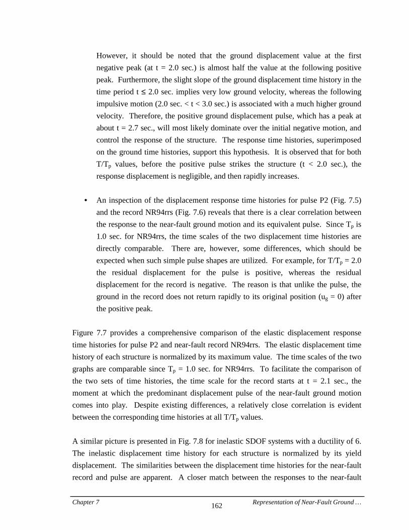
Chapter 7 Representation of Near-Fault Ground … 162
However, it should be noted that the ground displacement value at the first negative peak (at t = 2.0 sec.) is almost half the value at the following positive peak. Furthermore, the slight slope of the ground displacement time history in the time period t ≤ 2.0 sec. implies very low ground velocity, whereas the following impulsive motion (2.0 sec. < t < 3.0 sec.) is associated with a much higher ground velocity. Therefore, the positive ground displacement pulse, which has a peak at about t = 2.7 sec., will most likely dominate over the initial negative motion, and control the response of the structure. The response time histories, superimposed on the ground time histories, support this hypothesis. It is observed that for both T/Tp values, before the positive pulse strikes the structure (t < 2.0 sec.), the response displacement is negligible, and then rapidly increases.
• = An inspection of the displacement response time histories for pulse P2 (Fig. 7.5)
and the record NR94rrs (Fig. 7.6) reveals that there is a clear correlation between the response to the near-fault ground motion and its equivalent pulse. Since Tp is 1.0 sec. for NR94rrs, the time scales of the two displacement time histories are directly comparable. There are, however, some differences, which should be expected when such simple pulse shapes are utilized. For example, for T/Tp = 2.0 the residual displacement for the pulse is positive, whereas the residual displacement for the record is negative. The reason is that unlike the pulse, the ground in the record does not return rapidly to its original position (ug = 0) after the positive peak.
Figure 7.7 provides a comprehensive comparison of the elastic displacement response time histories for pulse P2 and near-fault record NR94rrs. The elastic displacement time history of each structure is normalized by its maximum value. The time scales of the two graphs are comparable since Tp = 1.0 sec. for NR94rrs. To facilitate the comparison of the two sets of time histories, the time scale for the record starts at t = 2.1 sec., the moment at which the predominant displacement pulse of the near-fault ground motion comes into play. Despite existing differences, a relatively close correlation is evident between the corresponding time histories at all T/Tp values. A similar picture is presented in Fig. 7.8 for inelastic SDOF systems with a ductility of 6. The inelastic displacement time history for each structure is normalized by its yield displacement. The similarities between the displacement time histories for the near-fault record and pulse are apparent. A closer match between the responses to the near-fault
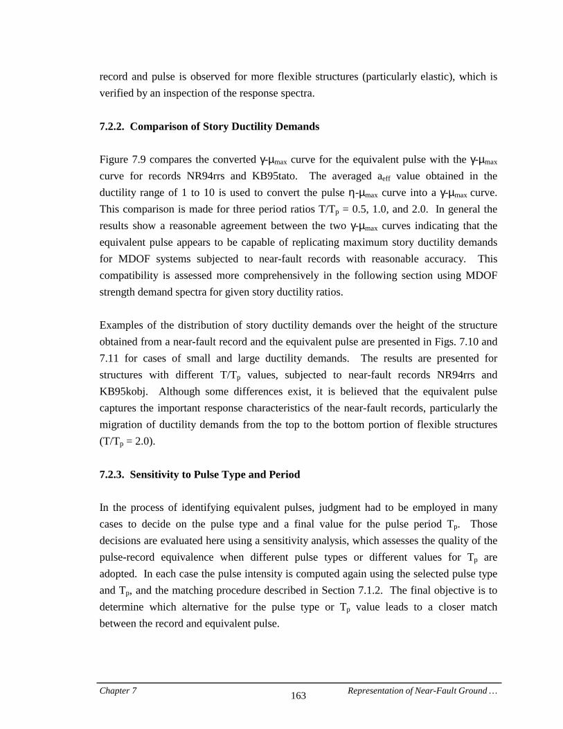
Chapter 7 Representation of Near-Fault Ground … 163
record and pulse is observed for more flexible structures (particularly elastic), which is verified by an inspection of the response spectra. 7.2.2. Comparison of Story Ductility Demands Figure 7.9 compares the converted γ-µmax curve for the equivalent pulse with the γ-µmax curve for records NR94rrs and KB95tato. The averaged aeff value obtained in the ductility range of 1 to 10 is used to convert the pulse η-µmax curve into a γ-µmax curve. This comparison is made for three period ratios T/Tp = 0.5, 1.0, and 2.0. In general the results show a reasonable agreement between the two γ-µmax curves indicating that the equivalent pulse appears to be capable of replicating maximum story ductility demands for MDOF systems subjected to near-fault records with reasonable accuracy. This compatibility is assessed more comprehensively in the following section using MDOF strength demand spectra for given story ductility ratios. Examples of the distribution of story ductility demands over the height of the structure obtained from a near-fault record and the equivalent pulse are presented in Figs. 7.10 and 7.11 for cases of small and large ductility demands. The results are presented for structures with different T/Tp values, subjected to near-fault records NR94rrs and KB95kobj. Although some differences exist, it is believed that the equivalent pulse captures the important response characteristics of the near-fault records, particularly the migration of ductility demands from the top to the bottom portion of flexible structures (T/Tp = 2.0). 7.2.3. Sensitivity to Pulse Type and Period In the process of identifying equivalent pulses, judgment had to be employed in many cases to decide on the pulse type and a final value for the pulse period Tp. Those decisions are evaluated here using a sensitivity analysis, which assesses the quality of the pulse-record equivalence when different pulse types or different values for Tp are adopted. In each case the pulse intensity is computed again using the selected pulse type and Tp, and the matching procedure described in Section 7.1.2. The final objective is to determine which alternative for the pulse type or Tp value leads to a closer match between the record and equivalent pulse.
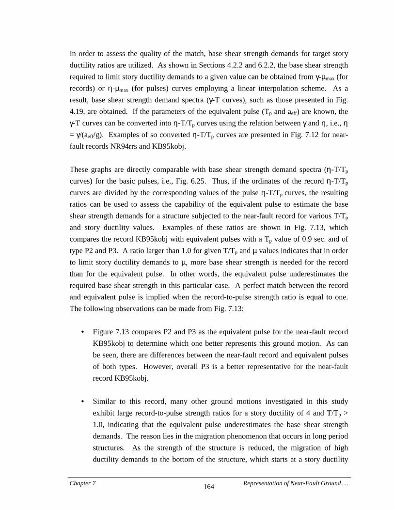
Chapter 7 Representation of Near-Fault Ground … 164
In order to assess the quality of the match, base shear strength demands for target story ductility ratios are utilized. As shown in Sections 4.2.2 and 6.2.2, the base shear strength required to limit story ductility demands to a given value can be obtained from γ-µmax (for records) or η-µmax (for pulses) curves employing a linear interpolation scheme. As a result, base shear strength demand spectra (γ-T curves), such as those presented in Fig. 4.19, are obtained. If the parameters of the equivalent pulse (Tp and aeff) are known, the γ-T curves can be converted into η-T/Tp curves using the relation between γ and η, i.e., η = γ/(aeff/g). Examples of so converted η-T/Tp curves are presented in Fig. 7.12 for near-fault records NR94rrs and KB95kobj. These graphs are directly comparable with base shear strength demand spectra (η-T/Tp curves) for the basic pulses, i.e., Fig. 6.25. Thus, if the ordinates of the record η-T/Tp curves are divided by the corresponding values of the pulse η-T/Tp curves, the resulting ratios can be used to assess the capability of the equivalent pulse to estimate the base shear strength demands for a structure subjected to the near-fault record for various T/Tp and story ductility values. Examples of these ratios are shown in Fig. 7.13, which compares the record KB95kobj with equivalent pulses with a Tp value of 0.9 sec. and of type P2 and P3. A ratio larger than 1.0 for given T/Tp and µ values indicates that in order to limit story ductility demands to µ, more base shear strength is needed for the record than for the equivalent pulse. In other words, the equivalent pulse underestimates the required base shear strength in this particular case. A perfect match between the record and equivalent pulse is implied when the record-to-pulse strength ratio is equal to one. The following observations can be made from Fig. 7.13:
• = Figure 7.13 compares P2 and P3 as the equivalent pulse for the near-fault record KB95kobj to determine which one better represents this ground motion. As can be seen, there are differences between the near-fault record and equivalent pulses of both types. However, overall P3 is a better representative for the near-fault record KB95kobj.
• = Similar to this record, many other ground motions investigated in this study
exhibit large record-to-pulse strength ratios for a story ductility of 4 and T/Tp > 1.0, indicating that the equivalent pulse underestimates the base shear strength demands. The reason lies in the migration phenomenon that occurs in long period structures. As the strength of the structure is reduced, the migration of high ductility demands to the bottom of the structure, which starts at a story ductility
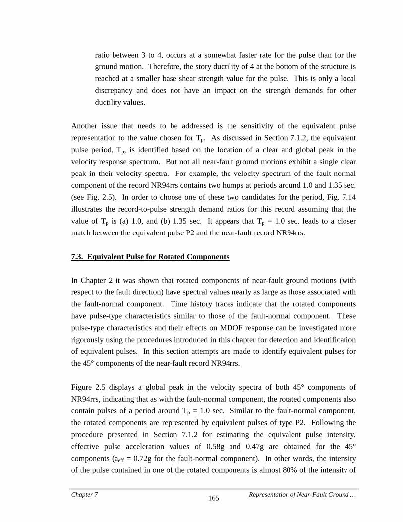
Chapter 7 Representation of Near-Fault Ground … 165
ratio between 3 to 4, occurs at a somewhat faster rate for the pulse than for the ground motion. Therefore, the story ductility of 4 at the bottom of the structure is reached at a smaller base shear strength value for the pulse. This is only a local discrepancy and does not have an impact on the strength demands for other ductility values.
Another issue that needs to be addressed is the sensitivity of the equivalent pulse representation to the value chosen for Tp. As discussed in Section 7.1.2, the equivalent pulse period, Tp, is identified based on the location of a clear and global peak in the velocity response spectrum. But not all near-fault ground motions exhibit a single clear peak in their velocity spectra. For example, the velocity spectrum of the fault-normal component of the record NR94rrs contains two humps at periods around 1.0 and 1.35 sec. (see Fig. 2.5). In order to choose one of these two candidates for the period, Fig. 7.14 illustrates the record-to-pulse strength demand ratios for this record assuming that the value of Tp is (a) 1.0, and (b) 1.35 sec. It appears that Tp = 1.0 sec. leads to a closer match between the equivalent pulse P2 and the near-fault record NR94rrs. 7.3. Equivalent Pulse for Rotated Components In Chapter 2 it was shown that rotated components of near-fault ground motions (with respect to the fault direction) have spectral values nearly as large as those associated with the fault-normal component. Time history traces indicate that the rotated components have pulse-type characteristics similar to those of the fault-normal component. These pulse-type characteristics and their effects on MDOF response can be investigated more rigorously using the procedures introduced in this chapter for detection and identification of equivalent pulses. In this section attempts are made to identify equivalent pulses for the 45° components of the near-fault record NR94rrs. Figure 2.5 displays a global peak in the velocity spectra of both 45° components of NR94rrs, indicating that as with the fault-normal component, the rotated components also contain pulses of a period around Tp = 1.0 sec. Similar to the fault-normal component, the rotated components are represented by equivalent pulses of type P2. Following the procedure presented in Section 7.1.2 for estimating the equivalent pulse intensity, effective pulse acceleration values of 0.58g and 0.47g are obtained for the 45° components (aeff = 0.72g for the fault-normal component). In other words, the intensity of the pulse contained in one of the rotated components is almost 80% of the intensity of
Chapter 7 Representation of Near-Fault Ground … 166
the pulse contained in the fault-normal component. This signifies that 45° components of near-fault records may still be quite severe. Figure 7.15 presents the record-to-pulse strength demand ratios for the rotated components of NR94rrs to illustrate the quality of the match between these records and the equivalent pulses identified previously. A comparison of these results with those corresponding to the fault-normal component (Fig. 7.14(a)) reveals that the response characteristics of the rotated record with aeff = 0.58 are very similar to those of the fault-normal component. Furthermore, this rotated component is relatively well represented by the equivalent pulse. 7.4. Estimation of Structure Response to Near-Fault Ground Motions An accurate evaluation of structure response to near-fault ground motions requires dynamic analyses that are computationally expensive. Since every near-fault record has unique properties, the response results for one ground motion are not useful in evaluating the response to a different ground motion. The equivalence established in this chapter between near-fault ground motions and simple pulses can be utilized in order to estimate seismic demands for MDOF structures with little effort. A multi-step procedure is presented in this section that can be used to estimate maximum story ductility, roof drift, and story drift angle demands for a given frame structure subjected to a specific near-fault record. The response of structures to simple pulses presented in Chapter 6 provides basic information for this procedure, which consists of the following steps:
1. Obtain the following structural properties: • = Fundamental period, T • = Base shear strength coefficient, γ = Vy/W
2. Obtain the following ground motion properties:
• = Peak ground velocity, PGV • = Pulse type (from the time history and spectral shapes, see Section 7.1.2) • = Pulse period, Tp (from the velocity spectrum, see Section 7.1.2) • = Pulse intensity, aeff = 4veff/Tp (use veff = PGV)
Chapter 7 Representation of Near-Fault Ground … 167
3. Calculate the following quantities: • = Period ratio, T/Tp • = Pulse strength parameter, η = (g/aeff)γ
Presuming that the given near-fault ground motion is best represented by pulse P2, the demands for structures subjected to P2, as presented in Chapter 6, are used to estimate seismic demands as follows:
4. Using the T/Tp and η values obtained in step 3, estimate the maximum story ductility demands from Fig. 7.16 (repetition of part of Fig. 6.21). For T/Tp values between those given in the graph, the maximum story ductility demand can be obtained using linear interpolation.
5. Using the T/Tp and η values, and computing ug,max = PGV.Tp/4, estimate the roof
displacement demand, δroof,max, from Fig. 7.17 (repetition of Fig. 6.32). For T/Tp values between those given in the graph, the roof displacement demand can be obtained using linear interpolation.
6. Using the T/Tp and η values, estimate story drift demands, ui, as follows:
• = Calculate roof drift angle, θroof = δroof,max/H, where H is the structure height.
• = Obtain the drift angle ratio for the story under consideration, λ = θi/θroof, from Fig. 7.18. Interpolate for T/Tp values between those given in the graphs.
• = Calculate ui = λhiθroof, where hi is the height of the story under consideration.
It is important to note that P-delta effects are not accounted for in the figures referred to in this section. While maximum story ductility demands and especially roof displacement demands are not very sensitive to the number of stories, the distribution of story drift demands over the height can be significantly affected by the number of stories (see Section 6.5). Therefore, for structures with a small number of stories, Fig. 7.18, which represents demands for a 20-story structure, may not provide a good estimate of the story drift demand. Figure 6.45 helps to provide improved estimates for structures with fewer than 20 stories.
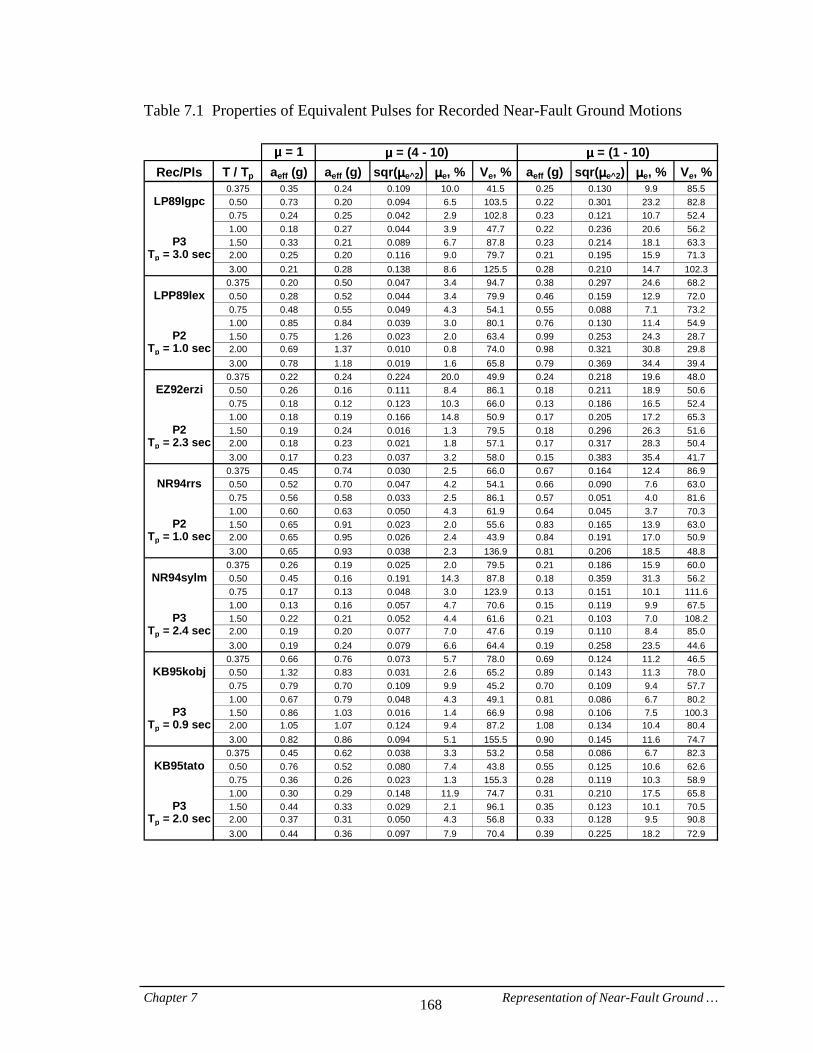
Chapter 7 Representation of Near-Fault Ground … 168
Table 7.1 Properties of Equivalent Pulses for Recorded Near-Fault Ground Motions
µµµµ = 1Rec/Pls T / Tp aeff (g) aeff (g) sqr(µµµµe^2) µµµµe, % Ve, % aeff (g) sqr(µµµµe^2) µµµµe, % Ve, %
0.375 0.35 0.24 0.109 10.0 41.5 0.25 0.130 9.9 85.5LP89lgpc 0.50 0.73 0.20 0.094 6.5 103.5 0.22 0.301 23.2 82.8
0.75 0.24 0.25 0.042 2.9 102.8 0.23 0.121 10.7 52.41.00 0.18 0.27 0.044 3.9 47.7 0.22 0.236 20.6 56.2
P3 1.50 0.33 0.21 0.089 6.7 87.8 0.23 0.214 18.1 63.3Tp = 3.0 sec 2.00 0.25 0.20 0.116 9.0 79.7 0.21 0.195 15.9 71.3
3.00 0.21 0.28 0.138 8.6 125.5 0.28 0.210 14.7 102.30.375 0.20 0.50 0.047 3.4 94.7 0.38 0.297 24.6 68.2
LPP89lex 0.50 0.28 0.52 0.044 3.4 79.9 0.46 0.159 12.9 72.00.75 0.48 0.55 0.049 4.3 54.1 0.55 0.088 7.1 73.21.00 0.85 0.84 0.039 3.0 80.1 0.76 0.130 11.4 54.9
P2 1.50 0.75 1.26 0.023 2.0 63.4 0.99 0.253 24.3 28.7Tp = 1.0 sec 2.00 0.69 1.37 0.010 0.8 74.0 0.98 0.321 30.8 29.8
3.00 0.78 1.18 0.019 1.6 65.8 0.79 0.369 34.4 39.40.375 0.22 0.24 0.224 20.0 49.9 0.24 0.218 19.6 48.0
EZ92erzi 0.50 0.26 0.16 0.111 8.4 86.1 0.18 0.211 18.9 50.60.75 0.18 0.12 0.123 10.3 66.0 0.13 0.186 16.5 52.41.00 0.18 0.19 0.166 14.8 50.9 0.17 0.205 17.2 65.3
P2 1.50 0.19 0.24 0.016 1.3 79.5 0.18 0.296 26.3 51.6Tp = 2.3 sec 2.00 0.18 0.23 0.021 1.8 57.1 0.17 0.317 28.3 50.4
3.00 0.17 0.23 0.037 3.2 58.0 0.15 0.383 35.4 41.70.375 0.45 0.74 0.030 2.5 66.0 0.67 0.164 12.4 86.9
NR94rrs 0.50 0.52 0.70 0.047 4.2 54.1 0.66 0.090 7.6 63.00.75 0.56 0.58 0.033 2.5 86.1 0.57 0.051 4.0 81.61.00 0.60 0.63 0.050 4.3 61.9 0.64 0.045 3.7 70.3
P2 1.50 0.65 0.91 0.023 2.0 55.6 0.83 0.165 13.9 63.0Tp = 1.0 sec 2.00 0.65 0.95 0.026 2.4 43.9 0.84 0.191 17.0 50.9
3.00 0.65 0.93 0.038 2.3 136.9 0.81 0.206 18.5 48.80.375 0.26 0.19 0.025 2.0 79.5 0.21 0.186 15.9 60.0
NR94sylm 0.50 0.45 0.16 0.191 14.3 87.8 0.18 0.359 31.3 56.20.75 0.17 0.13 0.048 3.0 123.9 0.13 0.151 10.1 111.61.00 0.13 0.16 0.057 4.7 70.6 0.15 0.119 9.9 67.5
P3 1.50 0.22 0.21 0.052 4.4 61.6 0.21 0.103 7.0 108.2Tp = 2.4 sec 2.00 0.19 0.20 0.077 7.0 47.6 0.19 0.110 8.4 85.0
3.00 0.19 0.24 0.079 6.6 64.4 0.19 0.258 23.5 44.60.375 0.66 0.76 0.073 5.7 78.0 0.69 0.124 11.2 46.5
KB95kobj 0.50 1.32 0.83 0.031 2.6 65.2 0.89 0.143 11.3 78.00.75 0.79 0.70 0.109 9.9 45.2 0.70 0.109 9.4 57.71.00 0.67 0.79 0.048 4.3 49.1 0.81 0.086 6.7 80.2
P3 1.50 0.86 1.03 0.016 1.4 66.9 0.98 0.106 7.5 100.3Tp = 0.9 sec 2.00 1.05 1.07 0.124 9.4 87.2 1.08 0.134 10.4 80.4
3.00 0.82 0.86 0.094 5.1 155.5 0.90 0.145 11.6 74.70.375 0.45 0.62 0.038 3.3 53.2 0.58 0.086 6.7 82.3
KB95tato 0.50 0.76 0.52 0.080 7.4 43.8 0.55 0.125 10.6 62.60.75 0.36 0.26 0.023 1.3 155.3 0.28 0.119 10.3 58.91.00 0.30 0.29 0.148 11.9 74.7 0.31 0.210 17.5 65.8
P3 1.50 0.44 0.33 0.029 2.1 96.1 0.35 0.123 10.1 70.5Tp = 2.0 sec 2.00 0.37 0.31 0.050 4.3 56.8 0.33 0.128 9.5 90.8
3.00 0.44 0.36 0.097 7.9 70.4 0.39 0.225 18.2 72.9
µµµµ = (1 - 10)µµµµ = (4 - 10)
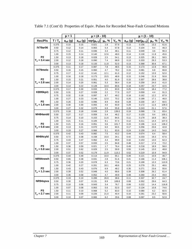
Chapter 7 Representation of Near-Fault Ground … 169
Table 7.1 (Cont’d) Properties of Equiv. Pulses for Recorded Near-Fault Ground Motions
µµµµ = 1Rec/Pls T / Tp aeff (g) aeff (g) sqr(µµµµe^2) µµµµe, % Ve, % aeff (g) sqr(µµµµe^2) µµµµe, % Ve, %
0.375 0.10 0.15 0.021 1.8 57.9 0.13 0.156 13.3 61.6IV79ar06 0.50 0.12 0.14 0.063 5.4 57.8 0.13 0.104 9.4 46.3
0.75 0.12 0.11 0.036 3.3 48.1 0.11 0.049 3.6 90.31.00 0.15 0.14 0.140 12.6 48.0 0.14 0.130 11.8 45.6
P2 1.50 0.13 0.18 0.028 2.5 54.1 0.13 0.325 28.1 58.5Tp = 3.4 sec 2.00 0.12 0.18 0.090 7.4 68.9 0.13 0.333 29.3 53.3
3.00 0.13 0.18 0.133 11.8 52.0 0.13 0.368 30.6 67.10.375 0.11 0.17 0.087 7.8 48.5 0.15 0.173 12.8 90.6
IV79melo 0.50 0.16 0.15 0.060 4.7 78.2 0.15 0.081 6.8 66.80.75 0.17 0.12 0.141 12.1 61.0 0.12 0.152 13.5 52.01.00 0.16 0.18 0.173 15.5 48.9 0.15 0.246 21.9 50.8
P2 1.50 0.15 0.21 0.051 4.0 81.9 0.15 0.307 28.6 38.8Tp = 2.8 sec 2.00 0.14 0.20 0.061 5.3 58.4 0.16 0.259 24.0 41.0
3.00 0.14 0.22 0.128 10.0 80.6 0.18 0.257 23.7 42.50.375 0.17 0.30 0.033 2.5 83.9 0.25 0.232 18.4 77.2
KB95kpi1 0.50 0.31 0.27 0.028 2.2 77.0 0.27 0.059 4.4 91.30.75 0.32 0.18 0.097 8.7 49.2 0.18 0.162 12.2 87.91.00 0.27 0.23 0.146 12.0 70.2 0.20 0.189 17.1 46.0
P2 1.50 0.26 0.33 0.096 8.9 40.8 0.28 0.230 19.7 60.5Tp = 1.8 sec 2.00 0.30 0.30 0.055 4.0 93.9 0.29 0.172 11.6 109.3
3.00 0.27 0.32 0.079 6.9 55.8 0.26 0.243 21.1 57.60.375 0.18 0.18 0.049 2.9 139.0 0.19 0.099 7.6 83.4
MH84andd 0.50 0.27 0.17 0.059 5.4 46.2 0.17 0.133 9.4 100.10.75 0.14 0.10 0.153 11.6 84.5 0.11 0.179 16.8 38.31.00 0.21 0.11 0.105 9.1 57.4 0.12 0.211 14.4 107.0
P2 1.50 0.21 0.16 0.051 3.6 101.7 0.15 0.196 11.6 136.2Tp = 0.8 sec 2.00 0.13 0.21 0.070 6.0 60.5 0.17 0.256 23.6 42.8
3.00 0.19 0.27 0.066 5.1 83.9 0.24 0.159 14.0 54.80.375 0.42 0.43 0.082 7.5 43.2 0.44 0.074 6.4 58.4
MH84cyld 0.50 0.72 0.38 0.158 15.0 34.1 0.42 0.233 19.3 67.60.75 0.43 0.47 0.062 4.4 99.9 0.42 0.153 13.0 62.31.00 0.37 0.57 0.033 2.5 84.8 0.48 0.217 17.6 72.2
P3 1.50 0.36 0.59 0.021 1.7 76.4 0.49 0.218 18.9 58.0Tp = 0.8 sec 2.00 0.51 0.62 0.029 2.5 59.9 0.55 0.145 13.0 48.8
3.00 0.37 0.52 0.179 11.9 113.2 0.52 0.219 15.9 94.90.375 0.44 0.49 0.114 10.0 55.1 0.49 0.121 10.9 46.7
NR94newh 0.50 0.65 0.38 0.031 2.8 51.6 0.41 0.166 11.4 106.10.75 0.36 0.20 0.078 6.3 73.6 0.21 0.199 13.3 110.91.00 0.42 0.27 0.201 18.1 48.6 0.25 0.279 25.1 48.6
P2 1.50 0.43 0.43 0.076 6.9 48.2 0.35 0.271 23.6 55.6Tp = 1.3 sec 2.00 0.39 0.52 0.048 4.0 68.6 0.39 0.308 26.2 61.4
3.00 0.36 0.58 0.052 4.7 49.9 0.48 0.260 23.4 49.00.375 0.19 0.10 0.289 26.9 38.6 0.11 0.337 32.7 24.7
NR94spva 0.50 0.30 0.07 0.131 8.9 108.8 0.08 0.352 29.6 64.30.75 0.10 0.06 0.043 3.4 76.7 0.06 0.222 14.4 116.81.00 0.07 0.08 0.063 5.6 52.0 0.07 0.134 10.8 74.6
P3 1.50 0.11 0.10 0.068 5.2 83.0 0.10 0.080 6.2 82.5Tp = 2.7 sec 2.00 0.11 0.09 0.226 21.0 40.4 0.10 0.261 23.2 50.6
3.00 0.10 0.07 0.065 6.2 29.6 0.08 0.097 8.5 52.9
µµµµ = (1 - 10)µµµµ = (4 - 10)
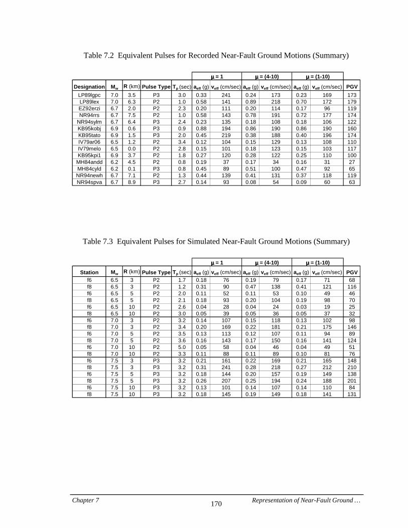
Chapter 7 Representation of Near-Fault Ground … 170
Table 7.2 Equivalent Pulses for Recorded Near-Fault Ground Motions (Summary)
Designation Mw R (km) Pulse Type Tp (sec) aeff (g) veff (cm/sec) aeff (g) veff (cm/sec) aeff (g) veff (cm/sec) PGVLP89lgpc 7.0 3.5 P3 3.0 0.33 241 0.24 173 0.23 169 173LP89lex 7.0 6.3 P2 1.0 0.58 141 0.89 218 0.70 172 179EZ92erzi 6.7 2.0 P2 2.3 0.20 111 0.20 114 0.17 96 119NR94rrs 6.7 7.5 P2 1.0 0.58 143 0.78 191 0.72 177 174
NR94sylm 6.7 6.4 P3 2.4 0.23 135 0.18 108 0.18 106 122KB95kobj 6.9 0.6 P3 0.9 0.88 194 0.86 190 0.86 190 160KB95tato 6.9 1.5 P3 2.0 0.45 219 0.38 188 0.40 196 174IV79ar06 6.5 1.2 P2 3.4 0.12 104 0.15 129 0.13 108 110IV79melo 6.5 0.0 P2 2.8 0.15 101 0.18 123 0.15 103 117KB95kpi1 6.9 3.7 P2 1.8 0.27 120 0.28 122 0.25 110 100
MH84andd 6.2 4.5 P2 0.8 0.19 37 0.17 34 0.16 31 27MH84cyld 6.2 0.1 P3 0.8 0.45 89 0.51 100 0.47 92 65NR94newh 6.7 7.1 P2 1.3 0.44 139 0.41 131 0.37 118 119NR94spva 6.7 8.9 P3 2.7 0.14 93 0.08 54 0.09 60 63
µµµµ = 1 µµµµ = (1-10)µµµµ = (4-10)
Table 7.3 Equivalent Pulses for Simulated Near-Fault Ground Motions (Summary)
Station Mw R (km) Pulse Type Tp (sec) aeff (g) veff (cm/sec) aeff (g) veff (cm/sec) aeff (g) veff (cm/sec) PGVf6 6.5 3 P2 1.7 0.18 76 0.19 79 0.17 71 68f8 6.5 3 P2 1.2 0.31 90 0.47 138 0.41 121 116f6 6.5 5 P2 2.0 0.11 52 0.11 53 0.10 49 46f8 6.5 5 P2 2.1 0.18 93 0.20 104 0.19 98 70f6 6.5 10 P2 2.6 0.04 28 0.04 24 0.03 19 25f8 6.5 10 P2 3.0 0.05 39 0.05 36 0.05 37 32f6 7.0 3 P2 3.2 0.14 107 0.15 118 0.13 102 98f8 7.0 3 P2 3.4 0.20 169 0.22 181 0.21 175 146f6 7.0 5 P2 3.5 0.13 113 0.12 107 0.11 94 89f8 7.0 5 P2 3.6 0.16 143 0.17 150 0.16 141 124f6 7.0 10 P2 5.0 0.05 58 0.04 46 0.04 49 51f8 7.0 10 P2 3.3 0.11 88 0.11 89 0.10 81 76f6 7.5 3 P3 3.2 0.21 161 0.22 169 0.21 165 148f8 7.5 3 P3 3.2 0.31 241 0.28 218 0.27 212 210f6 7.5 5 P3 3.2 0.18 144 0.20 157 0.19 149 138f8 7.5 5 P3 3.2 0.26 207 0.25 194 0.24 188 201f6 7.5 10 P3 3.2 0.13 101 0.14 107 0.14 110 84f8 7.5 10 P3 3.2 0.18 145 0.19 149 0.18 141 131
µµµµ = 1 µµµµ = (1-10)µµµµ = (4-10)
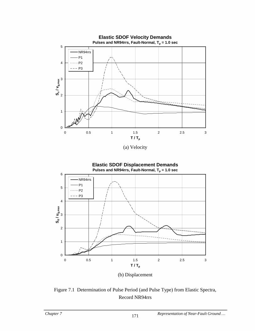
Chapter 7 Representation of Near-Fault Ground … 171
Elastic SDOF Velocity DemandsPulses and NR94rrs, Fault-Normal, Tp = 1.0 sec
0
1
2
3
4
5
0 0.5 1 1.5 2 2.5 3T / Tp
S v /
v g,m
ax
NR94rrsP1P2P3
(a) Velocity
Elastic SDOF Displacement DemandsPulses and NR94rrs, Fault-Normal, Tp = 1.0 sec
0
1
2
3
4
5
6
0 0.5 1 1.5 2 2.5 3T / Tp
S d /
u g,m
ax
NR94rrsP1P2P3
(b) Displacement
Figure 7.1 Determination of Pulse Period (and Pulse Type) from Elastic Spectra,
Record NR94rrs
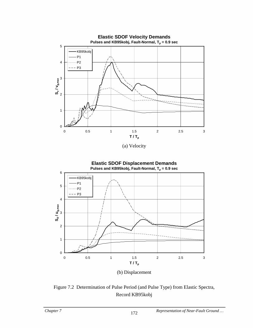
Chapter 7 Representation of Near-Fault Ground … 172
Elastic SDOF Velocity DemandsPulses and KB95kobj, Fault-Normal, Tp = 0.9 sec
0
1
2
3
4
5
0 0.5 1 1.5 2 2.5 3T / Tp
S v /
v g,m
ax
KB95kobjP1P2P3
(a) Velocity
Elastic SDOF Displacement DemandsPulses and KB95kobj, Fault-Normal, Tp = 0.9 sec
0
1
2
3
4
5
6
0 0.5 1 1.5 2 2.5 3T / Tp
S d /
u g,m
ax
KB95kobjP1P2P3
(b) Displacement
Figure 7.2 Determination of Pulse Period (and Pulse Type) from Elastic Spectra,
Record KB95kobj

Chapter 7 Representation of Near-Fault Ground … 173
Elastic SDOF Velocity DemandsPulses and KB95tato, Fault-Normal, Tp = 2.0 sec
0
1
2
3
4
5
0 0.5 1 1.5 2 2.5 3T / Tp
S v /
v g,m
ax
KB95tatoP1P2P3
(a) Velocity
Elastic SDOF Displacement DemandsPulses and KB95tato, Fault-Normal, Tp = 2.0 sec
0
1
2
3
4
5
6
0 0.5 1 1.5 2 2.5 3T / Tp
S d /
u g,m
ax
KB95tatoP1P2P3
(b) Displacement
Figure 7.3 Determination of Pulse Period (and Pulse Type) from Elastic Spectra,
Record KB95tato
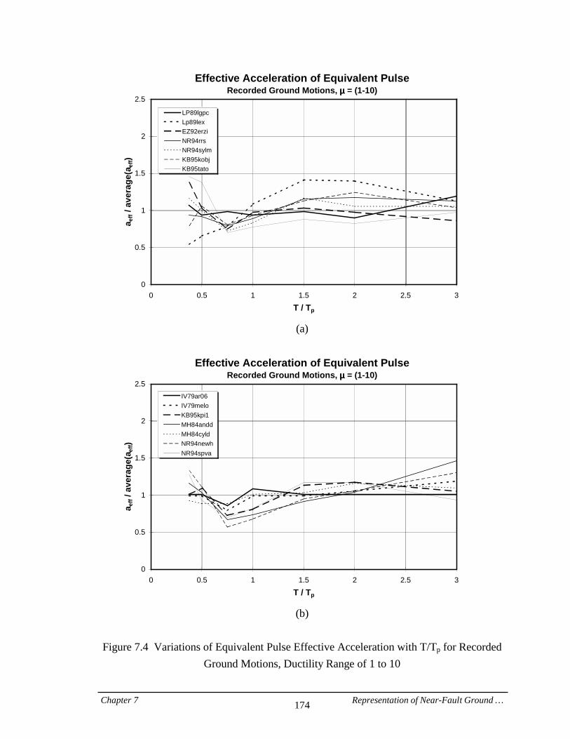
Chapter 7 Representation of Near-Fault Ground … 174
Effective Acceleration of Equivalent PulseRecorded Ground Motions, µµµµ = (1-10)
0
0.5
1
1.5
2
2.5
0 0.5 1 1.5 2 2.5 3T / Tp
a eff
/ ave
rage
(aef
f)
LP89lgpcLp89lexEZ92erziNR94rrsNR94sylmKB95kobjKB95tato
(a)
Effective Acceleration of Equivalent Pulse
Recorded Ground Motions, µµµµ = (1-10)
0
0.5
1
1.5
2
2.5
0 0.5 1 1.5 2 2.5 3T / Tp
a eff
/ ave
rage
(aef
f)
IV79ar06IV79meloKB95kpi1MH84anddMH84cyldNR94newhNR94spva
(b)
Figure 7.4 Variations of Equivalent Pulse Effective Acceleration with T/Tp for Recorded
Ground Motions, Ductility Range of 1 to 10
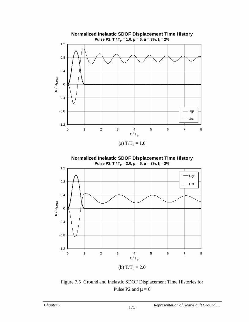
Chapter 7 Representation of Near-Fault Ground … 175
Normalized Inelastic SDOF Displacement Time HistoryPulse P2, T / Tp = 1.0, µµµµ = 6, αααα = 3%, ξξξξ = 2%
-1.2
-0.8
-0.4
0
0.4
0.8
1.2
0 1 2 3 4 5 6 7 8t / Tp
u / u
g,m
ax
Ugr
Ust
(a) T/Tp = 1.0
Normalized Inelastic SDOF Displacement Time History
Pulse P2, T / Tp = 2.0, µµµµ = 6, αααα = 3%, ξξξξ = 2%
-1.2
-0.8
-0.4
0
0.4
0.8
1.2
0 1 2 3 4 5 6 7 8t / Tp
u / u
g,m
ax
Ugr
Ust
(b) T/Tp = 2.0
Figure 7.5 Ground and Inelastic SDOF Displacement Time Histories for
Pulse P2 and µ = 6
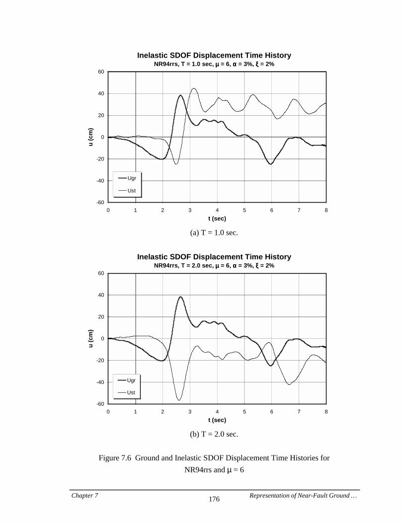
Chapter 7 Representation of Near-Fault Ground … 176
Inelastic SDOF Displacement Time HistoryNR94rrs, T = 1.0 sec, µµµµ = 6, αααα = 3%, ξξξξ = 2%
-60
-40
-20
0
20
40
60
0 1 2 3 4 5 6 7 8t (sec)
u (c
m)
Ugr
Ust
(a) T = 1.0 sec.
Inelastic SDOF Displacement Time History
NR94rrs, T = 2.0 sec, µµµµ = 6, αααα = 3%, ξξξξ = 2%
-60
-40
-20
0
20
40
60
0 1 2 3 4 5 6 7 8t (sec)
u (c
m)
Ugr
Ust
(b) T = 2.0 sec.
Figure 7.6 Ground and Inelastic SDOF Displacement Time Histories for
NR94rrs and µ = 6
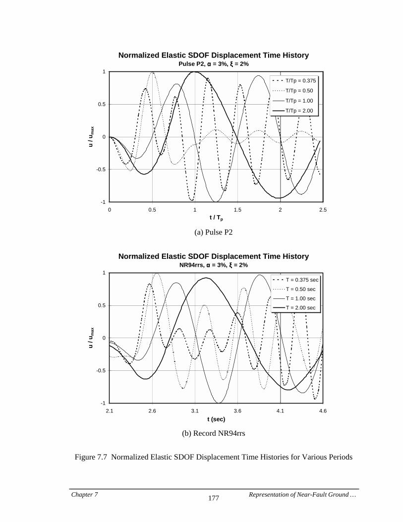
Chapter 7 Representation of Near-Fault Ground … 177
Normalized Elastic SDOF Displacement Time HistoryPulse P2, αααα = 3%, ξξξξ = 2%
-1
-0.5
0
0.5
1
0 0.5 1 1.5 2 2.5t / Tp
u / u
max
T/Tp = 0.375
T/Tp = 0.50
T/Tp = 1.00
T/Tp = 2.00
(a) Pulse P2
Normalized Elastic SDOF Displacement Time History
NR94rrs, αααα = 3%, ξξξξ = 2%
-1
-0.5
0
0.5
1
2.1 2.6 3.1 3.6 4.1 4.6t (sec)
u / u
max
T = 0.375 sec
T = 0.50 sec
T = 1.00 sec
T = 2.00 sec
(b) Record NR94rrs
Figure 7.7 Normalized Elastic SDOF Displacement Time Histories for Various Periods
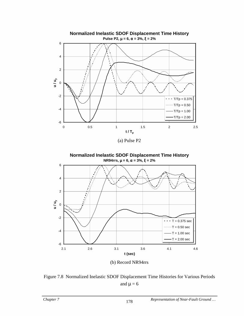
Chapter 7 Representation of Near-Fault Ground … 178
Normalized Inelastic SDOF Displacement Time HistoryPulse P2, µµµµ = 6, αααα = 3%, ξξξξ = 2%
-6
-4
-2
0
2
4
6
0 0.5 1 1.5 2 2.5t / Tp
u / u
y
T/Tp = 0.375
T/Tp = 0.50
T/Tp = 1.00
T/Tp = 2.00
(a) Pulse P2
Normalized Inelastic SDOF Displacement Time History
NR94rrs, µµµµ = 6, αααα = 3%, ξξξξ = 2%
-6
-4
-2
0
2
4
6
2.1 2.6 3.1 3.6 4.1 4.6t (sec)
u / u
y
T = 0.375 sec
T = 0.50 sec
T = 1.00 sec
T = 2.00 sec
(b) Record NR94rrs
Figure 7.8 Normalized Inelastic SDOF Displacement Time Histories for Various Periods
and µ = 6
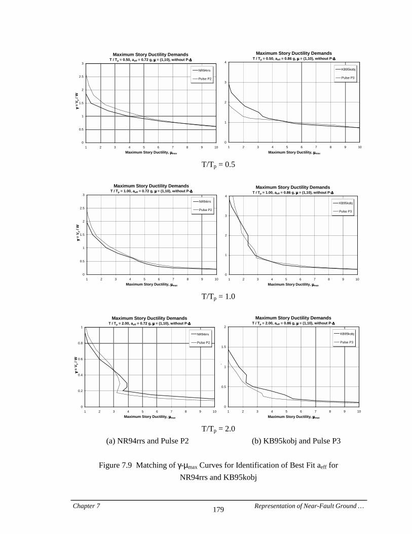
Chapter 7 Representation of Near-Fault Ground … 179
Maximum Story Ductility Demands T / Tp = 0.50, aeff = 0.72 g, µµµµ = (1,10), without P-∆∆∆∆
0
0.5
1
1.5
2
2.5
3
1 2 3 4 5 6 7 8 9 10Maximum Story Ductility, µµµµmax
γγ γγ =
V y /
WNR94rrs
Pulse P2
Maximum Story Ductility Demands T / Tp = 0.50, aeff = 0.86 g, µµµµ = (1,10), without P-∆∆∆∆
0
1
2
3
4
1 2 3 4 5 6 7 8 9 10Maximum Story Ductility, µµµµmax
y
KB95kobj
Pulse P3
T/Tp = 0.5
Maximum Story Ductility Demands
T / Tp = 1.00, aeff = 0.72 g, µµµµ = (1,10), without P-∆∆∆∆
0
0.5
1
1.5
2
2.5
3
1 2 3 4 5 6 7 8 9 10Maximum Story Ductility, µµµµmax
γγ γγ =
V y /
W
NR94rrs
Pulse P2
Maximum Story Ductility Demands T / Tp = 1.00, aeff = 0.86 g, µµµµ = (1,10), without P-∆∆∆∆
0
1
2
3
4
1 2 3 4 5 6 7 8 9 10Maximum Story Ductility, µµµµmax
KB95kobj
Pulse P3
T/Tp = 1.0
Maximum Story Ductility Demands
T / Tp = 2.00, aeff = 0.72 g, µµµµ = (1,10), without P-∆∆∆∆
0
0.2
0.4
0.6
0.8
1
1 2 3 4 5 6 7 8 9 10Maximum Story Ductility, µµµµmax
γγ γγ =
V y /
W
NR94rrs
Pulse P2
Maximum Story Ductility Demands T / Tp = 2.00, aeff = 0.86 g, µµµµ = (1,10), without P-∆∆∆∆
0
0.5
1
1.5
2
1 2 3 4 5 6 7 8 9 10Maximum Story Ductility, µµµµmax
γγ γγy
KB95kobj
Pulse P3
T/Tp = 2.0
(a) NR94rrs and Pulse P2 (b) KB95kobj and Pulse P3
Figure 7.9 Matching of γ-µmax Curves for Identification of Best Fit aeff for NR94rrs and KB95kobj
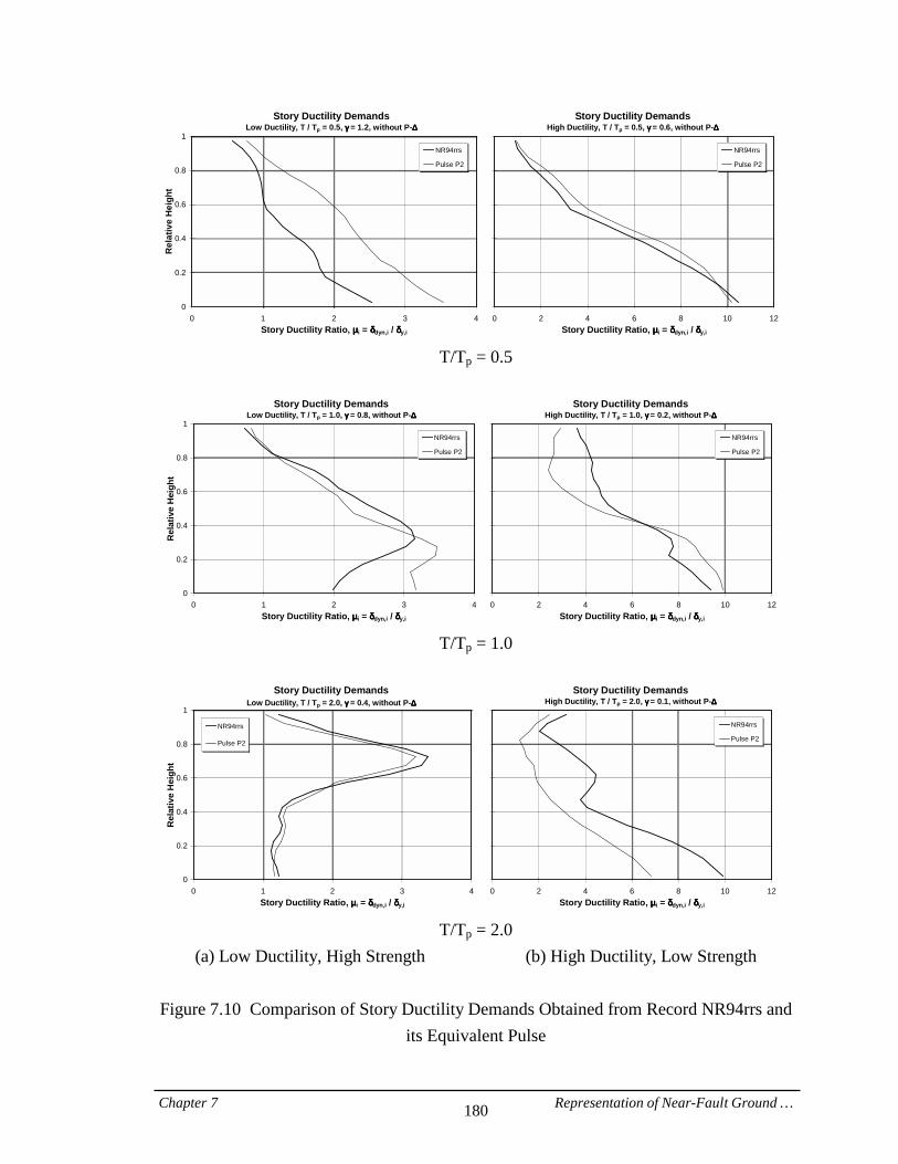
Chapter 7 Representation of Near-Fault Ground … 180
Story Ductility DemandsLow Ductility, T / Tp = 0.5, γγγγ = 1.2, without P-∆∆∆∆
0
0.2
0.4
0.6
0.8
1
0 1 2 3 4Story Ductility Ratio, µµµµi = δδδδdyn,i / δδδδy,i
Rel
ativ
e H
eigh
t
NR94rrs
Pulse P2
Story Ductility DemandsHigh Ductility, T / Tp = 0.5, γγγγ = 0.6, without P-∆∆∆∆
0 2 4 6 8 10 12Story Ductility Ratio, µµµµi = δδδδdyn,i / δδδδy,i
NR94rrs
Pulse P2
T/Tp = 0.5
Story Ductility Demands
Low Ductility, T / Tp = 1.0, γγγγ = 0.8, without P-∆∆∆∆
0
0.2
0.4
0.6
0.8
1
0 1 2 3 4Story Ductility Ratio, µµµµi = δδδδdyn,i / δδδδy,i
Rel
ativ
e H
eigh
t
NR94rrs
Pulse P2
Story Ductility DemandsHigh Ductility, T / Tp = 1.0, γγγγ = 0.2, without P-∆∆∆∆
0 2 4 6 8 10 12Story Ductility Ratio, µµµµi = δδδδdyn,i / δδδδy,i
NR94rrs
Pulse P2
T/Tp = 1.0
Story Ductility Demands
Low Ductility, T / Tp = 2.0, γγγγ = 0.4, without P-∆∆∆∆
0
0.2
0.4
0.6
0.8
1
0 1 2 3 4Story Ductility Ratio, µµµµi = δδδδdyn,i / δδδδy,i
Rel
ativ
e H
eigh
t
NR94rrs
Pulse P2
Story Ductility DemandsHigh Ductility, T / Tp = 2.0, γγγγ = 0.1, without P-∆∆∆∆
0 2 4 6 8 10 12Story Ductility Ratio, µµµµi = δδδδdyn,i / δδδδy,i
NR94rrs
Pulse P2
T/Tp = 2.0
(a) Low Ductility, High Strength (b) High Ductility, Low Strength
Figure 7.10 Comparison of Story Ductility Demands Obtained from Record NR94rrs and its Equivalent Pulse
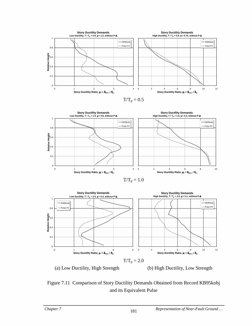
Chapter 7 Representation of Near-Fault Ground … 181
Story Ductility DemandsLow Ductility, T / Tp = 0.5, γγγγ = 1.2, without P-∆∆∆∆
0
0.2
0.4
0.6
0.8
1
0 1 2 3 4Story Ductility Ratio, µµµµi = δδδδdyn,i / δδδδy,i
Rel
ativ
e H
eigh
t
KB95kobj
Pulse P3
Story Ductility DemandsHigh Ductility, T / Tp = 0.5, γγγγ = 0.75, without P-∆∆∆∆
0 2 4 6 8 10 12Story Ductility Ratio, µµµµi = δδδδdyn,i / δδδδy,i
KB95kobj
Pulse P3
T/Tp = 0.5
Story Ductility Demands
Low Ductility, T / Tp = 1.0, γγγγ = 0.8, without P-∆∆∆∆
0
0.2
0.4
0.6
0.8
1
0 1 2 3 4Story Ductility Ratio, µµµµi = δδδδdyn,i / δδδδy,i
Rel
ativ
e H
eigh
t
KB95kobj
Pulse P3
Story Ductility DemandsHigh Ductility, T / Tp = 1.0, γγγγ = 0.3, without P-∆∆∆∆
0 2 4 6 8 10Story Ductility Ratio, µµµµi = δδδδdyn,i / δδδδy,i
KB95kobj
Pulse P3
T/Tp = 1.0
Story Ductility Demands
Low Ductility, T / Tp = 2.0, γγγγ = 0.4, without P-∆∆∆∆
0
0.2
0.4
0.6
0.8
1
0 1 2 3 4Story Ductility Ratio, µµµµi = δδδδdyn,i / δδδδy,i
Rel
ativ
e H
eigh
t
KB95kobj
Pulse P3
Story Ductility DemandsHigh Ductility, T / Tp = 2.0, γγγγ = 0.1, without P-∆∆∆∆
0 2 4 6 8 10 12Story Ductility Ratio, µµµµi = δδδδdyn,i / δδδδy,i
KB95kobj
Pulse P3
T/Tp = 2.0
(a) Low Ductility, High Strength (b) High Ductility, Low Strength
Figure 7.11 Comparison of Story Ductility Demands Obtained from Record KB95kobj and its Equivalent Pulse
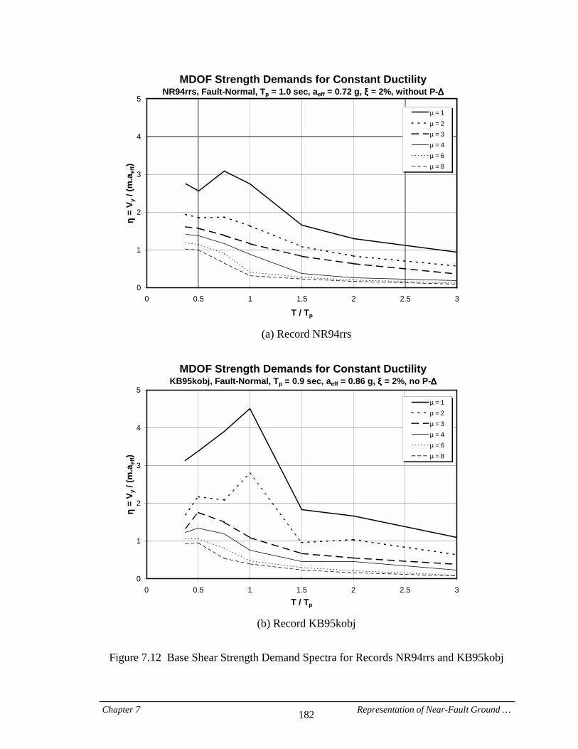
Chapter 7 Representation of Near-Fault Ground … 182
MDOF Strength Demands for Constant DuctilityNR94rrs, Fault-Normal, Tp = 1.0 sec, aeff = 0.72 g, ξξξξ = 2%, without P-∆∆∆∆
0
1
2
3
4
5
0 0.5 1 1.5 2 2.5 3
T / Tp
ηη ηη =
V y /
(m.a
eff)
µ===1
µ===2µ===3
µ===4µ===6
µ===8
(a) Record NR94rrs
MDOF Strength Demands for Constant Ductility
KB95kobj, Fault-Normal, Tp = 0.9 sec, aeff = 0.86 g, ξξξξ = 2%, no P-∆∆∆∆
0
1
2
3
4
5
0 0.5 1 1.5 2 2.5 3T / Tp
ηη ηη =
V y /
(m.a
eff)
µ===1
µ===2µ===3
µ===4µ===6
µ===8
(b) Record KB95kobj
Figure 7.12 Base Shear Strength Demand Spectra for Records NR94rrs and KB95kobj
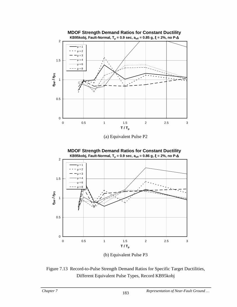
Chapter 7 Representation of Near-Fault Ground … 183
MDOF Strength Demand Ratios for Constant DuctilityKB95kobj, Fault-Normal, Tp = 0.9 sec, aeff = 0.85 g, ξξξξ = 2%, no P-∆∆∆∆
0
0.5
1
1.5
2
0 0.5 1 1.5 2 2.5 3T / Tp
ηη ηη NF== ==
// // == == ηη ηηP2
µ===1
µ===2
µ===3
µ===4
µ===6
µ===8
(a) Equivalent Pulse P2
MDOF Strength Demand Ratios for Constant Ductility
KB95kobj, Fault-Normal, Tp = 0.9 sec, aeff = 0.86 g, ξξξξ = 2%, no P-∆∆∆∆
0
0.5
1
1.5
2
0 0.5 1 1.5 2 2.5 3T / Tp
ηη ηη NF== ==
// // == == ηη ηηP3
µ===1
µ===2
µ===3
µ===4
µ===6
µ===8
(b) Equivalent Pulse P3
Figure 7.13 Record-to-Pulse Strength Demand Ratios for Specific Target Ductilities,
Different Equivalent Pulse Types, Record KB95kobj
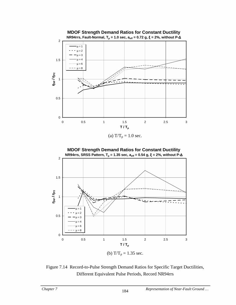
Chapter 7 Representation of Near-Fault Ground … 184
MDOF Strength Demand Ratios for Constant DuctilityNR94rrs, Fault-Normal, Tp = 1.0 sec, aeff = 0.72 g, ξξξξ = 2%, without P-∆∆∆∆
0
0.5
1
1.5
2
0 0.5 1 1.5 2 2.5 3T / Tp
ηη ηη NF== ==
// // == == ηη ηηP2
µ===1
µ===2
µ===3
µ===4
µ===6
µ===8
(a) T/Tp = 1.0 sec.
MDOF Strength Demand Ratios for Constant DuctilityNR94rrs, SRSS Pattern, Tp = 1.35 sec, aeff = 0.54 g, ξξξξ = 2%, without P-∆∆∆∆
0
0.5
1
1.5
2
0 0.5 1 1.5 2 2.5 3T / Tp
ηη ηη NF== ==
// // == == ηη ηηP2
µ===1
µ===2
µ===3
µ===4
µ===6
µ===8
(b) T/Tp = 1.35 sec.
Figure 7.14 Record-to-Pulse Strength Demand Ratios for Specific Target Ductilities,
Different Equivalent Pulse Periods, Record NR94rrs
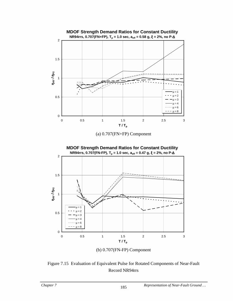
Chapter 7 Representation of Near-Fault Ground … 185
MDOF Strength Demand Ratios for Constant DuctilityNR94rrs, 0.707(FN+FP), Tp = 1.0 sec, aeff = 0.58 g, ξξξξ = 2%, no P-∆∆∆∆
0
0.5
1
1.5
2
0 0.5 1 1.5 2 2.5 3T / Tp
ηη ηη 45°=
= =
=
// // == == ηη ηηP2
µ===1µ===2µ===3µ===4µ===6µ===8
(a) 0.707(FN+FP) Component
MDOF Strength Demand Ratios for Constant Ductility
NR94rrs, 0.707(FN-FP), Tp = 1.0 sec, aeff = 0.47 g, ξξξξ = 2%, no P-∆∆∆∆
0
0.5
1
1.5
2
0 0.5 1 1.5 2 2.5 3T / Tp
ηη ηη 45°=
= =
=
// // == == ηη ηηP2
µ===1µ===2µ===3µ===4µ===6µ===8
(b) 0.707(FN-FP) Component
Figure 7.15 Evaluation of Equivalent Pulse for Rotated Components of Near-Fault
Record NR94rrs
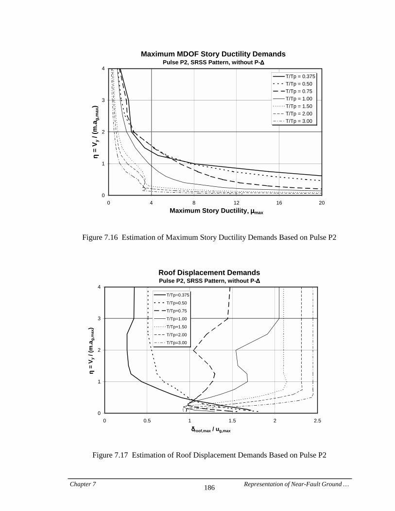
Chapter 7 Representation of Near-Fault Ground … 186
Maximum MDOF Story Ductility DemandsPulse P2, SRSS Pattern, without P-∆∆∆∆
0
1
2
3
4
0 4 8 12 16 20Maximum Story Ductility,,,,====µµµµmax
ηη ηη =
V y /
(m.a
g,m
ax)
T/Tp = 0.375T/Tp = 0.50T/Tp = 0.75T/Tp = 1.00T/Tp = 1.50T/Tp = 2.00T/Tp = 3.00
Figure 7.16 Estimation of Maximum Story Ductility Demands Based on Pulse P2
Roof Displacement DemandsPulse P2, SRSS Pattern, without P-∆∆∆∆
0
1
2
3
4
0 0.5 1 1.5 2 2.5δδδδroof,max / ug,max
ηη ηη =
V y /
(m.a
g,m
ax)
T/Tp=0.375
T/Tp=0.50
T/Tp=0.75
T/Tp=1.00
T/Tp=1.50
T/Tp=2.00
T/Tp=3.00
Figure 7.17 Estimation of Roof Displacement Demands Based on Pulse P2
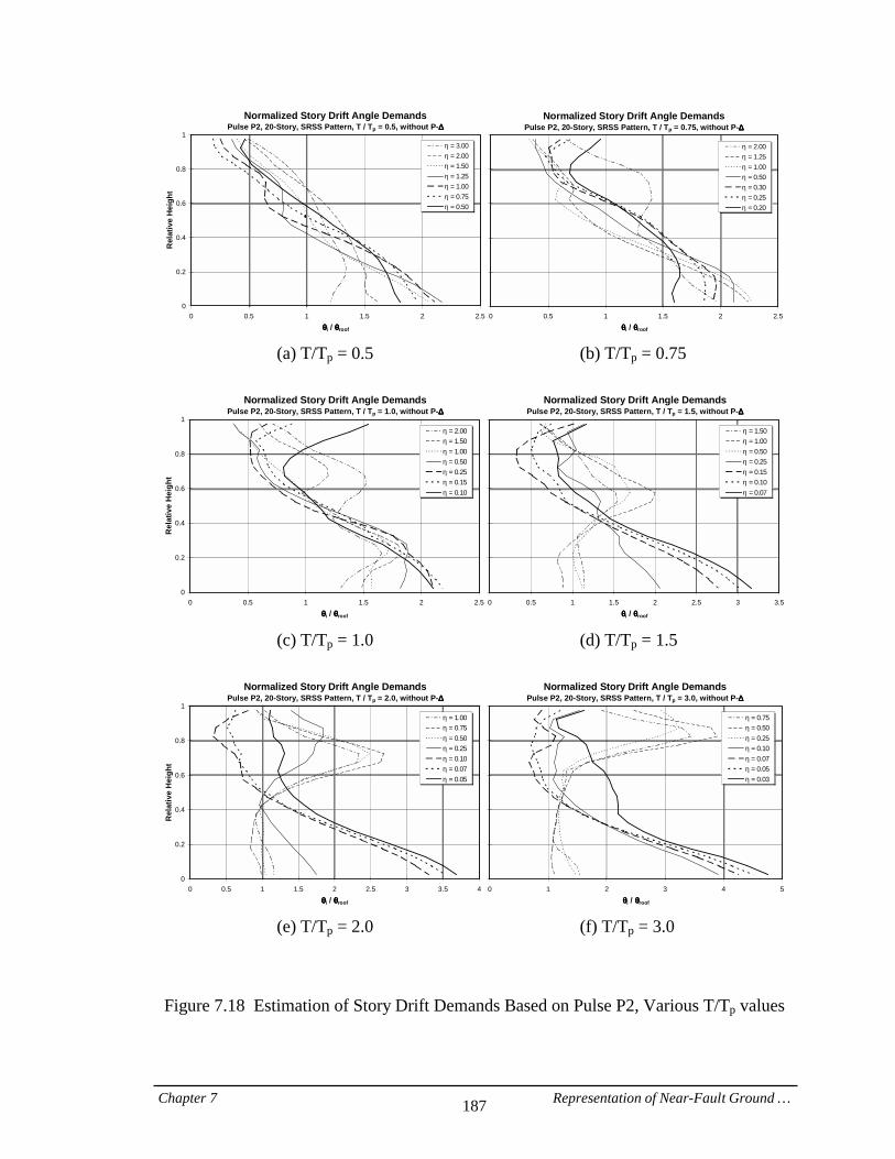
Chapter 7 Representation of Near-Fault Ground … 187
Normalized Story Drift Angle DemandsPulse P2, 20-Story, SRSS Pattern, T / Tp = 0.5, without P-∆∆∆∆
0
0.2
0.4
0.6
0.8
1
0 0.5 1 1.5 2 2.5θθθθi / θθθθroof
Rel
ativ
e H
eigh
t
η===3.00η===2.00η===1.50η===1.25η===1.00η===0.75η===0.50
Normalized Story Drift Angle DemandsPulse P2, 20-Story, SRSS Pattern, T / Tp = 0.75, without P-∆∆∆∆
0 0.5 1 1.5 2 2.5θθθθi / θθθθroof
η===2.00η===1.25η===1.00η===0.50η===0.30η===0.25η===0.20
(a) T/Tp = 0.5 (b) T/Tp = 0.75
Normalized Story Drift Angle Demands
Pulse P2, 20-Story, SRSS Pattern, T / Tp = 1.0, without P-∆∆∆∆
0
0.2
0.4
0.6
0.8
1
0 0.5 1 1.5 2 2.5θθθθi / θθθθroof
Rel
ativ
e H
eigh
t
η===2.00η===1.50η===1.00η===0.50η===0.25η===0.15η===0.10
Normalized Story Drift Angle DemandsPulse P2, 20-Story, SRSS Pattern, T / Tp = 1.5, without P-∆∆∆∆
0 0.5 1 1.5 2 2.5 3 3.5θθθθi / θθθθroof
η===1.50η===1.00η===0.50η===0.25η===0.15η===0.10η===0.07
(c) T/Tp = 1.0 (d) T/Tp = 1.5
Normalized Story Drift Angle Demands
Pulse P2, 20-Story, SRSS Pattern, T / Tp = 2.0, without P-∆∆∆∆
0
0.2
0.4
0.6
0.8
1
0 0.5 1 1.5 2 2.5 3 3.5 4θθθθi / θθθθroof
Rel
ativ
e H
eigh
t
η===1.00η===0.75η===0.50η===0.25η===0.10η===0.07η===0.05
Normalized Story Drift Angle DemandsPulse P2, 20-Story, SRSS Pattern, T / Tp = 3.0, without P-∆∆∆∆
0 1 2 3 4 5θθθθi / θθθθroof
η===0.75η===0.50η===0.25η===0.10η===0.07η===0.05η===0.03
(e) T/Tp = 2.0 (f) T/Tp = 3.0
Figure 7.18 Estimation of Story Drift Demands Based on Pulse P2, Various T/Tp values

Chapter 8 Study of Models of Steel Structures 188
CHAPTER 8
STUDY OF MODELS OF STEEL STRUCTURES
The results presented in the previous chapters will be of value only if the generic structures introduced in Section 3.2 can represent a variety of real-world MDOF frame structures. In addition to frame geometrical configuration parameters such as the number of bays and stories, span length, or story height, there are a large number of factors that differentiate the simple generic frames from real structures. The design of the generic frames is based on many simplifying assumptions that do not necessarily represent real conditions in all cases. For instance, contributions of panel zones, floor slabs, and non-structural elements to the stiffness and strength of the system are ignored, and the generic design is based on particular distributions of story stiffness and strength over the height of the structure. On the other hand, employing sophisticated structural models that can fully account for all existing elements and effects of the system is not practical in many cases. If advantage can be taken of generic structures to predict the seismic demands of real structures with reasonable accuracy, a great deal of computational time and effort can be saved. Therefore, it is important to assess the usefulness of predictions obtained from the generic structures for various seismic demand quantities. In this chapter the correlation between demands is investigated for the generic frames and more realistic structural models subjected to near-fault ground motions, in order to justify and validate the use of generic models in this study. 8.1. Models of Steel Structures Used in this Study Two steel moment resisting frame (SMRF) models (3- and 9-story) are utilized, which were thoroughly analyzed in a past study carried out as part of the SAC Steel Program (Gupta and Krawinkler, 1999). The 2-dimensional frame models, which are referred to

Chapter 8 Study of Models of Steel Structures 189
as “LA 3-story” and “LA 9-story”, correspond to the perimeter moment resisting frames of two office buildings located in Los Angeles. The buildings have been designed to meet all prevailing gravity, wind, and seismic requirements of UBC’94 guidelines. The geometrical configurations of these two models are illustrated in Fig. 8.1. The moment resisting frames are shown in solid bold lines in the plan views. The LA 3-story frame has four bays, while the LA 9-story frame contains five bays. Moreover, the LA 9-story structure has a basement, and is laterally restrained at the ground level. Most of the member sizes are controlled by drift rather than strength considerations. The sections used in the LA 3-story and LA 9-story frames are summarized in Table 8.1. All columns in the perimeter frames bend about the strong axis. In the analyses, expected yield stress values of 339 MPa (49.2 ksi) and 397 MPa (57.6 ksi) are used for beams and columns, respectively, rather than the nominal values of 248 MPa (36 ksi) and 345 Mpa (50 ksi). The structure models used in this study are bare frames of type M2 in the SAC project, in which the dimensions, stiffness, strength, and inelastic shear distortion of panel zones are considered. The panel zones are modeled using a combination of standard beam-column elements and trilinear rotational springs at each joint. All other contributions to strength and stiffness, such as those due to the floor slabs, gravity columns, simple (shear) connections, and nonstructural elements, are neglected. Even though the interior (gravity) frames, which include shear (simple) connections, are not modeled, second-order (P-delta) effects due to gravity loads on these frames are taken into account by linking a virtual column to the main frame, which carries the vertical loads tributary to the interior gravity frames. For more modeling details the reader is referred to Gupta and Krawinkler (1999). 8.2. Inelastic Static Analysis and Calibration of Generic Structures Inelastic static (pushover) analysis is utilized here to calibrate the properties of the generic frames such that their demands can be directly compared with those of the LA 3-story and LA 9-story structures. The 3-story and 9-story frames introduced in Section 6.5.1 are selected as generic counterparts of the LA 3-story and LA 9-story structures, respectively. In addition to the SRSS lateral load pattern discussed previously, the 1994 NEHRP load pattern with k = 2 is used here in the pushover analyses. In this load pattern, the lateral load applied to the i-th story of the frame is given as:

Chapter 8 Study of Models of Steel Structures 190
Fw h
w hVi
i i
j jj
n=
=
2
2
1
(8.1)
where hi and wi are the height (from the base) and seismically effective weight of the i-th floor, respectively, and V represents the base shear. The power k = 2 in the NEHRP load pattern will be too large for the design of a 3-story structure, but in this study it is used only to compare pushover curves for the generic and LA 3-story structures. The global pushover curves, i.e., normalized base shear force (base shear normalized by structure seismic weight, V/W) versus roof displacement are shown in Figs. 8.2 and 8.3 for the LA 3-story and LA 9-story structures. Each graph illustrates the global nonlinear behavior of the structure subjected to the SRSS and NEHRP load patterns with and without consideration of P-delta effects. The pushover curve for the LA 3-story structure exhibits a bilinear shape, which indicates that all plastic hinges develop within a relatively narrow range of displacement. On the other hand, the plastic hinge formation in the LA 9-story frame occurs over a much wider range of displacement, resulting in a smoother transition from elastic behavior to a mechanism. Furthermore, the SRSS load pattern leads to higher yield strengths compared to the NEHRP pattern. This illustrates the sensitivity of the inelastic static behavior of multi-story frame structures to the shape of load patterns employed in the pushover analysis. Even though a post-yield strain-hardening ratio of 3.0% is assigned at the element level, the global strain-hardening ratio amounts to about 3.7% for the LA 3-story frame, and 4.1% for the LA 9-story frame in the absence of P-delta effects. However, once second-order effects are taken into account, the global strain-hardening ratio decreases to 0.3% for the LA 3-story frame, and to negative values for LA 9-story. The reason is that the gravity load in the 3-story structure is not large enough to cause a negative post-yield stiffness, whereas for the 9-story frame, beyond a certain displacement value, negative post-yield slopes are observed. An indication of the significance of P-delta effects on the global behavior of frame structures can be obtained from the first story “stability coefficient” defined as:
θ11
1=
PVh
∆ (8.2)
Chapter 8 Study of Models of Steel Structures 191
where P is the total vertical gravity load, ∆1 is the elastic first-order drift in the first story caused by the base shear V, and h1 denotes the height of the first story. The value of θ1 for LA 3-story and LA 9-story structures is 3.4% and 7.1%, respectively. These values help to explain the difference in the post-yield stiffness of the two frames. For comparison purposes, the generic 3-story structure is tuned to have a fundamental period equal to the fundamental period of the LA 3-story structure, i.e., 0.99 sec. (without P-delta effects). Likewise, the generic 9-story structure with a fundamental period of 2.17 sec. is compared with the LA 9-story structure. Since the story strengths of the generic structures follow a distribution that is obtained from the SRSS load pattern, only the pushover curves that are based on the SRSS load pattern are used for strength calibration. Even though the pushover curves of the LA structures, unlike those of the generic frames, do not exhibit a distinct yield point, the base shear strength can be estimated from the intersection of the extended elastic and inelastic branches. This results in strength coefficient values γ = Vy/W = 0.35 and 0.21 for the generic 3- and 9-story structures, respectively. In order for the response of the generic frames to be comparable with the response of the SAC structures, P-delta effects should also be compatible between the two systems. For this purpose, the amount of the vertical load acting on the generic frame is determined such that the first story stability coefficient is equal to the corresponding value for the SAC structure, i.e., θ1 = 3.4% and 7.1% for the 3- and 9-story frames. However, this merely means that static P-delta effects in the first story of the SAC and generic frames are at the same level as long as the systems behave elastically. The stability coefficients in higher stories of the two structures are not necessarily identical. Besides, once plastic hinges form, the deflected shape of the structure will deviate from the elastic deflected shape, and therefore the distribution of secondary effects over the height of the structure may change significantly (Gupta and Krawinkler, 1999). Figures 8.4 and 8.5 compare the global pushover curves (base shear vs. roof displacement) for the calibrated generic structures with the corresponding pushover curves for the SAC structures under NEHRP and SRSS load patterns (a) ignoring P-delta effects, and (b) considering P-delta effects. A close correlation between the results of the SAC structures and their corresponding generic frames are observed, which demonstrates the similarities of their global static behavior in both elastic and inelastic ranges. The
Chapter 8 Study of Models of Steel Structures 192
reflection of these similarities in dynamic response at global and story levels is investigated in the following section. 8.3. Inelastic Dynamic Analysis In this section the dynamic response of the SAC structures to near-fault ground motions is compared with the response obtained from the generic models. The objective is to assess the degree to which the response of generic structures can be used to estimate the response of real frame structures to near-fault ground motions. 8.3.1. Roof Displacement Figure 8.6 compares roof displacement time histories for the generic and LA 3-story structures subjected to near-fault records LP89lex, and KB95tato, considering P-delta effects. As can be seen, the correlation is very good, which is not surprising when similarity of the pushover curves for these two structures is considered (see Fig. 8.4). Figure 8.7 compares the roof displacement time histories, in the same manner as Fig. 8.6, for the generic and LA 9-story structures. Again, a very close agreement between the responses of the SAC and generic structures is observed, indicating that the generic model can capture global dynamic response with good accuracy. In order to investigate the response differences between the SAC and generic structures at different performance (inelasticity) levels, the input ground motion (i.e., LP89lex) is scaled using an intensity multiplier. A sequence of dynamic analyses that utilizes the same record with gradually increasing intensity is called “incremental dynamic analysis” (IDA). Figure 8.8 illustrates the roof displacement demands for the generic and LA 3-story frames versus the intensity multiplier (which equals unity for the original record) (a) ignoring P-delta effects, and (b) accounting for P-delta effects. Figure 8.9 compares the generic and LA 9-story structures in the same manner. The following observations can be made:
• = Despite some differences between the roof displacement demands for the generic and LA 9-story structures in the presence of P-delta effects, the demands obtained from the generic models are close to those obtained from the SAC models. This demonstrates that generic structures can estimate the global demands (roof
Chapter 8 Study of Models of Steel Structures 193
displacement) with sufficient accuracy and much less computational effort compared to more realistic, but complicated, models.
• = When P-delta effects are taken into account, the roof displacement demand grows
more rapidly with the ground motion intensity. This decrease in the slope of the IDA curve is especially evident for the 9-story structures (see Fig. 8.9) whose post-yield stiffness is negative giving rise to large secondary effects.
• = The reason why the generic 9-story structure exhibits larger P-delta effects than
the LA 9-story structure is that it enters a negative stiffness range at a smaller global drift, see Fig. 8.5(b).
8.3.2. Story Drift Angles In order to avoid ambiguity associated with the definition of story yield drift, story drift angle demands (story drift demand divided by story height) rather than story ductility demands are used here to represent story-level displacement demands. To allow a direct comparison of structures with different heights, as discussed in Section 6.5.3, the drift angle demands are normalized by the roof drift angle (roof displacement divided by structure height). Figure 8.10 compares the normalized drift angle demands for the calibrated generic and LA 3-story structures subjected to records LP89lex and KB95tato in the presence of P-delta effects. The distribution of the demands over the height is almost uniform, which implies that the deflected shapes are close to a straight line. This is not surprising when it is considered that the response of the 3-story structures is mainly controlled by the first mode, and that the first mode shape is close to a straight line. The results show that the normalized drift angle demands for the generic and SAC structures are relatively close. This is an indication that the generic 3-story structure can be utilized to estimate story drift demands with good accuracy. Figure 8.11 compares normalized drift angle demands for the generic and LA 9-story structures in the same manner. Although some differences are observed, particularly in the bottom portion of the structure, the general patterns of the two distributions are similar. The results indicate that overall, the generic model can represent story drift angle

Chapter 8 Study of Models of Steel Structures 194
demands. However, it should be noted that the distribution of story drift angle demands over the height of the structure is dependent on the number of stories (see Fig. 6.45). If the input ground motion is scaled using an intensity multiplier, as in the previous section, the distributions of normalized story drift angle demands over the height of the structure can be investigated at different performance levels. Figures 8.12 and 8.13 compare these distributions for the SAC and generic structures subjected to the record LP89lex with P-delta effects. The following observations are made:
• = Figure 8.12 shows that for the generic and LA 3-story structures the distributions are not far from uniform, indicating that the deflected shapes are close to a straight line at all performance levels. For the generic structure the maximum drift demand occurs in the bottom story at high performance levels (low severity ground motion), whereas at low performance levels (severe ground motion) the maximum demand shifts to the top story. This upward shift of the maximum drift demand was also observed in the response of the generic 3-story structure to the basic pulse P2 (see Fig. 6.45). This effect, however, is not as clear in the response of the LA 3-story structure to the same near-fault ground motion.
• = Figure 8.13 illustrates the migration phenomenon for the generic and LA 9-story
structures, which was previously identified as a near-fault response characteristic of MDOF structures with T/Tp > 1.0 (T/Tp ≅ 2.2 in this case). That is, for low intensity ground motions (or strong structures) the maximum story drift demand occurs in the upper portion of the structure, and as the ground motion intensity increases (or the structure strength decreases), the maximum demand migrates to the bottom. Although the generic 9-story structure can overall capture the distribution of drift demands for the LA 9-story structure, at low performance levels the distributions are much less uniform for the SAC structure than for the generic one. The reason is that the story shear strengths of the SAC structures are not fine-tuned to the SRSS shear force distribution used to design the generic structure.
Summary: The results of the study presented in this chapter indicate that generic structural models can be utilized to estimate the global demands for MDOF structures with good accuracy.

Chapter 8 Study of Models of Steel Structures 195
However, due to the dependence of the distribution of story-level demands on the number of stories, as well as on the distribution of stiffness and strength over the height of the structure, estimating these demands from a single generic model, such as the generic 20-story frame used extensively in this study, should be done with caution and with due consideration to the peculiarities caused by subjective design decisions.
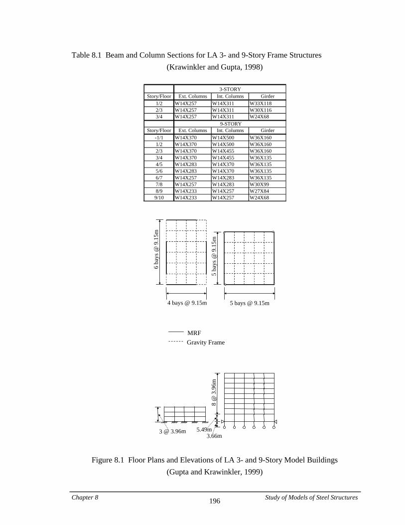
Chapter 8 Study of Models of Steel Structures 196
Table 8.1 Beam and Column Sections for LA 3- and 9-Story Frame Structures (Krawinkler and Gupta, 1998)
3-STORY
Story/Floor Ext. Columns Int. Columns Girder1/2 W14X257 W14X311 W33X1182/3 W14X257 W14X311 W30X1163/4 W14X257 W14X311 W24X68
9-STORYStory/Floor Ext. Columns Int. Columns Girder
-1/1 W14X370 W14X500 W36X1601/2 W14X370 W14X500 W36X1602/3 W14X370 W14X455 W36X1603/4 W14X370 W14X455 W36X1354/5 W14X283 W14X370 W36X1355/6 W14X283 W14X370 W36X1356/7 W14X257 W14X283 W36X1357/8 W14X257 W14X283 W30X998/9 W14X233 W14X257 W27X84
9/10 W14X233 W14X257 W24X68
4 bays @ 9.15m
6 ba
ys @
9.1
5m
5 bays @ 9.15m
5 ba
ys @
9.1
5m
3 @ 3.96m
8 @
3.9
6m
5.49m3.66m
MRFGravity Frame
Figure 8.1 Floor Plans and Elevations of LA 3- and 9-Story Model Buildings (Gupta and Krawinkler, 1999)
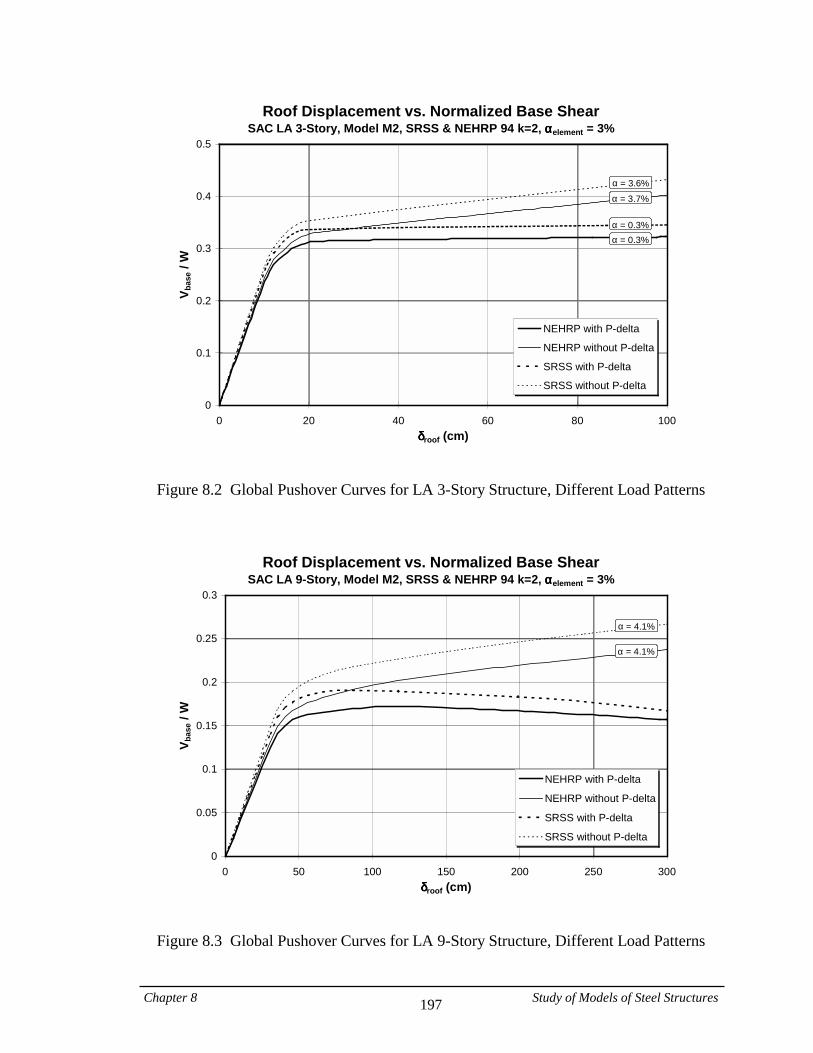
Chapter 8 Study of Models of Steel Structures 197
Roof Displacement vs. Normalized Base ShearSAC LA 3-Story, Model M2, SRSS & NEHRP 94 k=2, ααααelement = 3%
0
0.1
0.2
0.3
0.4
0.5
0 20 40 60 80 100δδδδroof (cm)
V bas
e / W
NEHRP with P-delta
NEHRP without P-delta
SRSS with P-delta
SRSS without P-delta
α = 3.6%α = 3.7%
α = 0.3%α = 0.3%
Figure 8.2 Global Pushover Curves for LA 3-Story Structure, Different Load Patterns
Roof Displacement vs. Normalized Base ShearSAC LA 9-Story, Model M2, SRSS & NEHRP 94 k=2, ααααelement = 3%
0
0.05
0.1
0.15
0.2
0.25
0.3
0 50 100 150 200 250 300δδδδroof (cm)
V bas
e / W
NEHRP with P-delta
NEHRP without P-delta
SRSS with P-delta
SRSS without P-delta
α = 4.1%
α = 4.1%
Figure 8.3 Global Pushover Curves for LA 9-Story Structure, Different Load Patterns

Chapter 8 Study of Models of Steel Structures 198
Roof Displacement vs. Normalized Base ShearGeneric and LA 3-Story, γγγγ = 0.35, without P-∆∆∆∆====
0
0.1
0.2
0.3
0.4
0.5
0 20 40 60 80 100δδδδroof (cm)
V bas
e / W
NEHRP, SAC
NEHRP, Generic
SRSS, SAC
SRSS, Generic
(a) without P-delta
Roof Displacement vs. Normalized Base Shear
Generic and LA 3-Story, γγγγ = 0.35, with P-∆∆∆∆====
0
0.1
0.2
0.3
0.4
0.5
0 20 40 60 80 100δδδδroof (cm)
V bas
e / W
NEHRP, SAC
NEHRP, Generic
SRSS, SAC
SRSS, Generic
(b) with P-delta
Figure 8.4 Comparison of Pushover Curves for Generic and LA 3-Story Structures
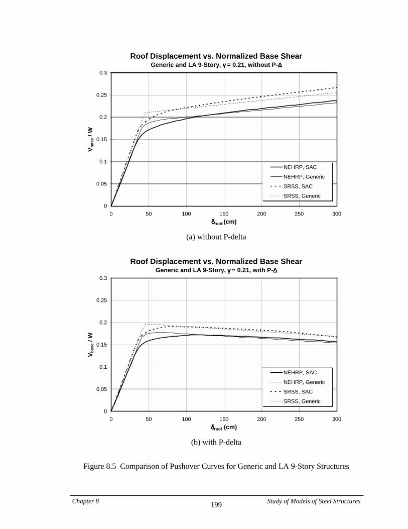
Chapter 8 Study of Models of Steel Structures 199
Roof Displacement vs. Normalized Base ShearGeneric and LA 9-Story, γγγγ = 0.21, without P-∆∆∆∆====
0
0.05
0.1
0.15
0.2
0.25
0.3
0 50 100 150 200 250 300δδδδroof (cm)
V bas
e / W
NEHRP, SAC
NEHRP, Generic
SRSS, SAC
SRSS, Generic
(a) without P-delta
Roof Displacement vs. Normalized Base Shear
Generic and LA 9-Story, γγγγ = 0.21, with P-∆∆∆∆====
0
0.05
0.1
0.15
0.2
0.25
0.3
0 50 100 150 200 250 300δδδδroof (cm)
V bas
e / W
NEHRP, SAC
NEHRP, Generic
SRSS, SAC
SRSS, Generic
(b) with P-delta
Figure 8.5 Comparison of Pushover Curves for Generic and LA 9-Story Structures
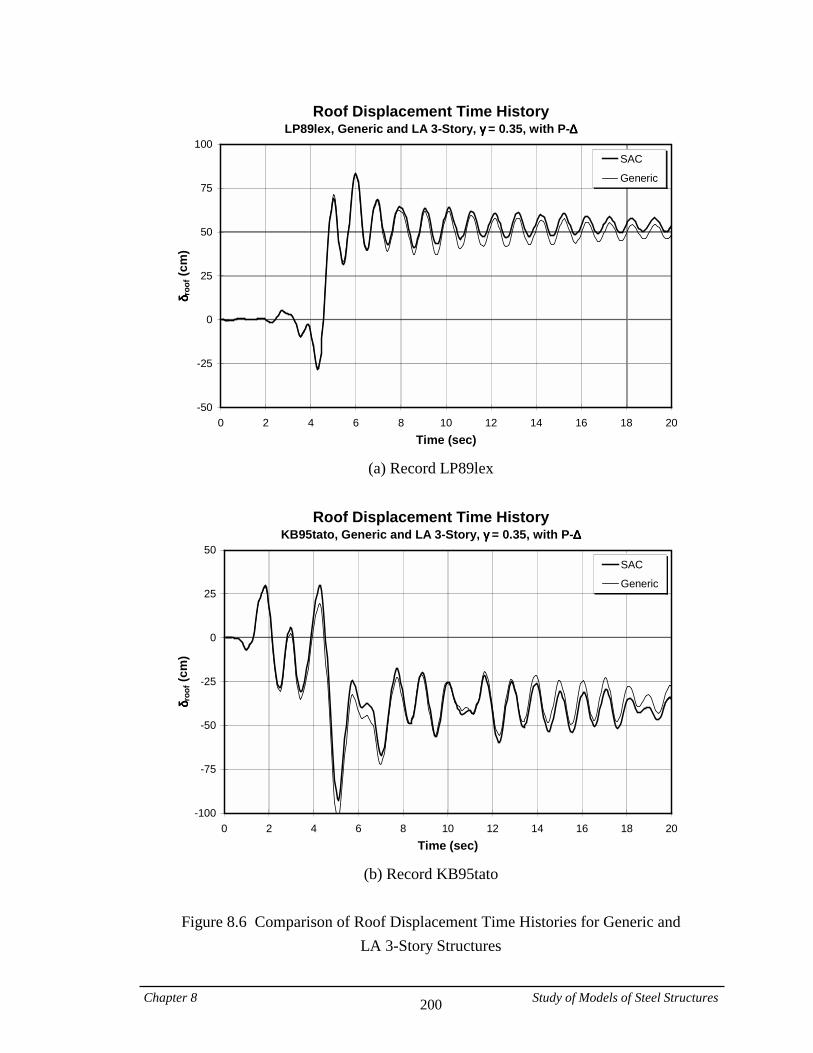
Chapter 8 Study of Models of Steel Structures 200
Roof Displacement Time HistoryLP89lex, Generic and LA 3-Story, γγγγ = 0.35, with P-∆∆∆∆====
-50
-25
0
25
50
75
100
0 2 4 6 8 10 12 14 16 18 20Time (sec)
δδ δδ roo
f (cm
)
SAC
Generic
(a) Record LP89lex
Roof Displacement Time History
KB95tato, Generic and LA 3-Story, γγγγ = 0.35, with P-∆∆∆∆====
-100
-75
-50
-25
0
25
50
0 2 4 6 8 10 12 14 16 18 20Time (sec)
δδ δδ roo
f (cm
)
SAC
Generic
(b) Record KB95tato
Figure 8.6 Comparison of Roof Displacement Time Histories for Generic and
LA 3-Story Structures
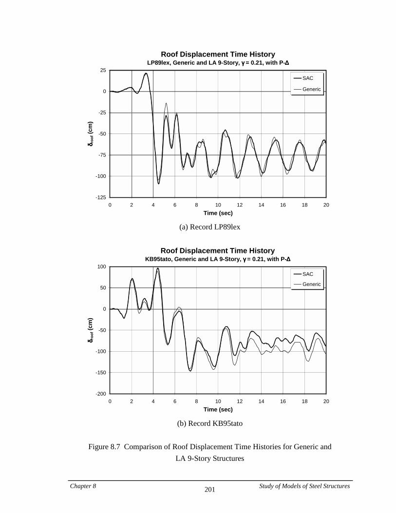
Chapter 8 Study of Models of Steel Structures 201
Roof Displacement Time HistoryLP89lex, Generic and LA 9-Story, γγγγ = 0.21, with P-∆∆∆∆====
-125
-100
-75
-50
-25
0
25
0 2 4 6 8 10 12 14 16 18 20Time (sec)
δδ δδ roo
f (cm
)
SAC
Generic
(a) Record LP89lex
Roof Displacement Time History
KB95tato, Generic and LA 9-Story, γγγγ = 0.21, with P-∆∆∆∆====
-200
-150
-100
-50
0
50
100
0 2 4 6 8 10 12 14 16 18 20Time (sec)
δδ δδ roo
f (cm
)
SAC
Generic
(b) Record KB95tato
Figure 8.7 Comparison of Roof Displacement Time Histories for Generic and
LA 9-Story Structures
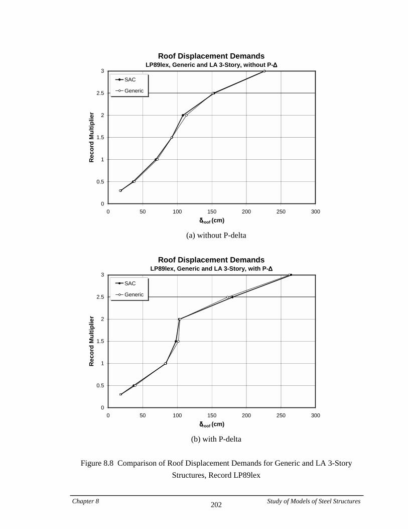
Chapter 8 Study of Models of Steel Structures 202
Roof Displacement DemandsLP89lex, Generic and LA 3-Story, without P-∆∆∆∆
0
0.5
1
1.5
2
2.5
3
0 50 100 150 200 250 300δδδδroof (cm)
Rec
ord
Mul
tiplie
r
SAC
Generic
(a) without P-delta
Roof Displacement Demands
LP89lex, Generic and LA 3-Story, with P-∆∆∆∆
0
0.5
1
1.5
2
2.5
3
0 50 100 150 200 250 300δδδδroof (cm)
Rec
ord
Mul
tiplie
r
SAC
Generic
(b) with P-delta
Figure 8.8 Comparison of Roof Displacement Demands for Generic and LA 3-Story
Structures, Record LP89lex
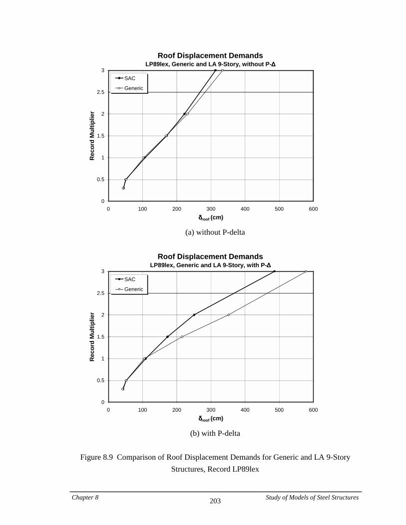
Chapter 8 Study of Models of Steel Structures 203
Roof Displacement DemandsLP89lex, Generic and LA 9-Story, without P-∆∆∆∆
0
0.5
1
1.5
2
2.5
3
0 100 200 300 400 500 600δδδδroof (cm)
Rec
ord
Mul
tiplie
r
SAC
Generic
(a) without P-delta
Roof Displacement Demands
LP89lex, Generic and LA 9-Story, with P-∆∆∆∆
0
0.5
1
1.5
2
2.5
3
0 100 200 300 400 500 600δδδδroof (cm)
Rec
ord
Mul
tiplie
r
SAC
Generic
(b) with P-delta
Figure 8.9 Comparison of Roof Displacement Demands for Generic and LA 9-Story
Structures, Record LP89lex
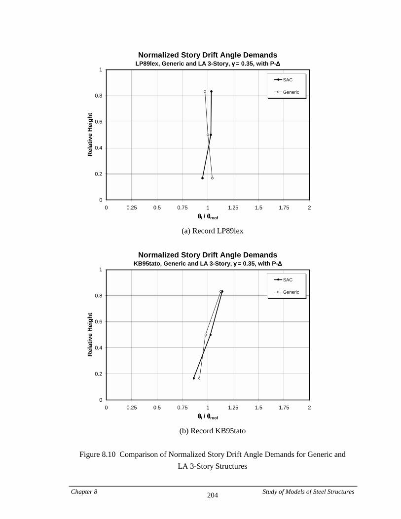
Chapter 8 Study of Models of Steel Structures 204
Normalized Story Drift Angle DemandsLP89lex, Generic and LA 3-Story, γγγγ = 0.35, with P-∆∆∆∆
0
0.2
0.4
0.6
0.8
1
0 0.25 0.5 0.75 1 1.25 1.5 1.75 2θθθθi / θθθθroof
Rel
ativ
e H
eigh
tSAC
Generic
(a) Record LP89lex
Normalized Story Drift Angle Demands
KB95tato, Generic and LA 3-Story, γγγγ = 0.35, with P-∆∆∆∆
0
0.2
0.4
0.6
0.8
1
0 0.25 0.5 0.75 1 1.25 1.5 1.75 2θθθθi / θθθθroof
Rel
ativ
e H
eigh
t
SAC
Generic
(b) Record KB95tato
Figure 8.10 Comparison of Normalized Story Drift Angle Demands for Generic and
LA 3-Story Structures
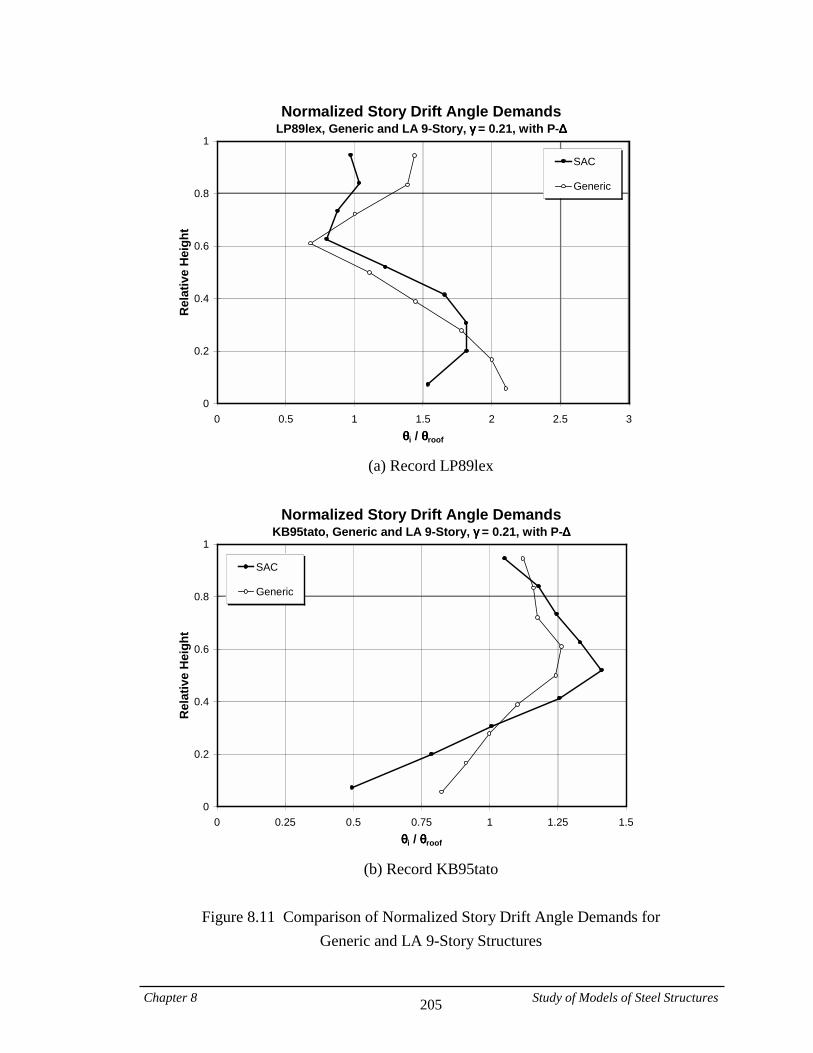
Chapter 8 Study of Models of Steel Structures 205
Normalized Story Drift Angle DemandsLP89lex, Generic and LA 9-Story, γγγγ = 0.21, with P-∆∆∆∆
0
0.2
0.4
0.6
0.8
1
0 0.5 1 1.5 2 2.5 3θθθθi / θθθθroof
Rel
ativ
e H
eigh
t
SAC
Generic
(a) Record LP89lex
Normalized Story Drift Angle Demands
KB95tato, Generic and LA 9-Story, γγγγ = 0.21, with P-∆∆∆∆
0
0.2
0.4
0.6
0.8
1
0 0.25 0.5 0.75 1 1.25 1.5θθθθi / θθθθroof
Rel
ativ
e H
eigh
t
SAC
Generic
(b) Record KB95tato
Figure 8.11 Comparison of Normalized Story Drift Angle Demands for
Generic and LA 9-Story Structures
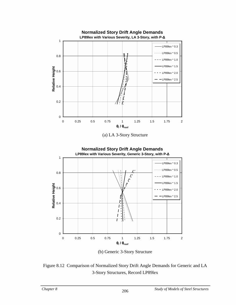
Chapter 8 Study of Models of Steel Structures 206
Normalized Story Drift Angle DemandsLP89lex with Various Severity, LA 3-Story, with P-∆∆∆∆
0
0.2
0.4
0.6
0.8
1
0 0.25 0.5 0.75 1 1.25 1.5 1.75 2θθθθi / θθθθroof
Rel
ativ
e H
eigh
t
LP89lex * 0.3
LP89lex * 0.5
LP89lex * 1.0
LP89lex * 1.5
LP89lex * 2.0
LP89lex * 2.5
(a) LA 3-Story Structure
Normalized Story Drift Angle Demands
LP89lex with Various Severity, Generic 3-Story, with P-∆∆∆∆
0
0.2
0.4
0.6
0.8
1
0 0.25 0.5 0.75 1 1.25 1.5 1.75 2θθθθi / θθθθroof
Rel
ativ
e H
eigh
t
LP89lex * 0.3
LP89lex * 0.5
LP89lex * 1.0
LP89lex * 1.5
LP89lex * 2.0
LP89lex * 2.5
(b) Generic 3-Story Structure
Figure 8.12 Comparison of Normalized Story Drift Angle Demands for Generic and LA
3-Story Structures, Record LP89lex
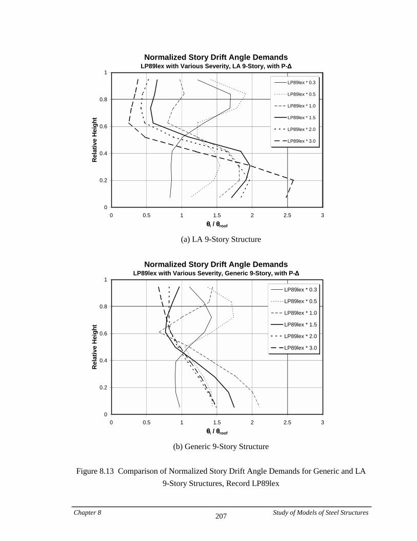
Chapter 8 Study of Models of Steel Structures 207
Normalized Story Drift Angle DemandsLP89lex with Various Severity, LA 9-Story, with P-∆∆∆∆
0
0.2
0.4
0.6
0.8
1
0 0.5 1 1.5 2 2.5 3θθθθi / θθθθroof
Rel
ativ
e H
eigh
t
LP89lex * 0.3
LP89lex * 0.5
LP89lex * 1.0
LP89lex * 1.5
LP89lex * 2.0
LP89lex * 3.0
(a) LA 9-Story Structure
Normalized Story Drift Angle Demands
LP89lex with Various Severity, Generic 9-Story, with P-∆∆∆∆
0
0.2
0.4
0.6
0.8
1
0 0.5 1 1.5 2 2.5 3θθθθi / θθθθroof
Rel
ativ
e H
eigh
t
LP89lex * 0.3
LP89lex * 0.5
LP89lex * 1.0
LP89lex * 1.5
LP89lex * 2.0
LP89lex * 3.0
(b) Generic 9-Story Structure
Figure 8.13 Comparison of Normalized Story Drift Angle Demands for Generic and LA
9-Story Structures, Record LP89lex
Chapter 9 Design Considerations for Near-Fault … 208
CHAPTER 9
DESIGN CONSIDERATIONS FOR NEAR-FAULT GROUND MOTIONS
In the previous chapters it was shown that structures designed according to current seismic guidelines might experience excessively large demands or undesirable distributions of demands over their height when subjected to near-fault ground motions. Various techniques are investigated in this chapter that can provide improved protection for frame structures located in the near-fault region of a seismic source. A summary is provided first of the results of a study that relates the parameters of the equivalent pulse discussed in Chapter 7 to earthquake moment magnitude, Mw, and closest distance to the fault rupture plane, R. Once these relationships are established, advantage is taken of the response of structures to simple pulse-type motions in order to evaluate the Mw and R dependence of seismic demands imposed by near-fault ground motions and to develop design recommendations. Strengthening techniques are investigated that serve to reduce the seismic demands either by modifying the distribution of story shear strength over the height of the structure or by adding walls of different properties to frame structures. The beneficial effects of strengthening with walls and the effects of different wall properties are discussed in detail. 9.1. Relationships Between Equivalent Pulse Parameters and Earthquake Magnitude and Distance In Chapter 7 it was demonstrated that within the period range of T/Tp from 0.375 to 3.0 it appears to be reasonable to represent near-fault ground motions by an equivalent pulse. Although not precise, such a representation is sufficiently accurate for practical purposes. The values of the equivalent pulse parameters were summarized in Tables 7.2 and 7.3 for the fault-normal component of the recorded and simulated near-fault ground motions with forward directivity used in this study. Regression analysis is performed on these
Chapter 9 Design Considerations for Near-Fault … 209
data to evaluate the magnitude (Mw) and distance (R) dependence of these parameters. Since relatively small sets of near-fault ground motions are available for this purpose, the results of such regression analysis should be interpreted with caution. 9.1.1. Pulse Period Somerville showed that the period of the pulse (Tp) contained in a near-fault ground motion is mostly affected by slip rise time, which is defined as the duration of slip at a given point on the fault (Somerville, 1998). He established a relationship between rise time and the moment magnitude (Mw) of the event. He also proposed a preliminary model that expresses log10Tp as a linear function of Mw, independent of distance. Employing the formulation proposed by Somerville for Tp and performing a linear regression analysis on equivalent pulse periods obtained for the combination of the recorded and simulated ground motions, the following regression equation is obtained: log10Tp = -1.76 + 0.31 Mw (9.1) Figure 9.1 illustrates this equation together with the data points (solid circles) to which the line is fitted for (a) log10Tp and (b) Tp. It should be noted that in this figure some of the circles represent more than one data point with identical Mw and Tp values. Two points corresponding to the recent Turkey and Taiwan earthquakes, which were not included in the regression analysis, are also shown. Superimposed on each graph are 90%, 80%, and 70% prediction bands for Tp, which illustrate the confidence levels for the regressed model. For example, for a given value of Mw, there is a 90% likelihood that the Tp value falls within the 90% prediction band that surrounds the regressed line. These prediction bands are obtained based on the assumption that the errors and the dependent parameter, i.e. log10Tp, are normally distributed (Ramsey and Schafer, 1996), which is to say that Tp follows a lognormal distribution with its median being the Tp value obtained from Eq. 9.1. If only pulse periods for the recorded ground motions are used in the regression analysis, the following equation is obtained: log10Tp = -2.06 + 0.34 Mw (9.2)
Chapter 9 Design Considerations for Near-Fault … 210
Figure 9.2 illustrates the same information as presented in Fig. 9.1, but for only the recorded ground motions. The following observations can be made from these figures:
• = The slopes of the regressed lines are very close for the two record sets, but the intercept is somewhat smaller for the recorded set, resulting in consistently smaller predictions based on the recorded set compared to the combined set of ground motions.
• = Large scatter in data points is observed for both record sets. In part this can be
attributed to the fact that the ground motions used in the regression analysis come from different events with different faulting mechanisms and geological conditions. The large scatter translates into wide prediction bands, which indicate large uncertainties in predicting Tp from the regression equations.
The large scatter may be interpreted as a lack of confidence in predicting Tp values from the regression equations. Later in Section 9.2 it will be investigated how a limited variation of Tp affects the base shear strength demands obtained from the equivalent pulse approach. As shown in figure 9.1, the right tail of the data used in the derivation of Eq. 9.1 consists of data points corresponding to one record from the Landers (1992) earthquake with magnitude 7.3 and six records from a simulated earthquake with magnitude 7.5 (with identical Tp). Any extrapolation beyond the magnitude range of the data points should be carried out with caution. The following example serves to evaluate to what extent the regression equation can be employed for large earthquakes. Somerville studied near-fault ground motions recorded in the magnitude 7.4 Izmit (Turkey, 1999) and magnitude 7.6 Chi-Chi (Taiwan, 1999) earthquakes (Somerville, 2000). Two of the pulse-type records used in his study are Yarimca (Turkey) and Tsaotun (Taiwan). The period of the pulse contained in the fault-normal component of these ground motions (from the location of a global peak in the velocity spectrum; see Somerville, 2000, for the spectra) is estimated to be 3.7 sec. and 4.2 sec., respectively. Figure 9.1 compares these values with those predicted by Eq. 9.1, indicating a good agreement.
Chapter 9 Design Considerations for Near-Fault … 211
9.1.2. Pulse Intensity Pulse effective velocity (veff = aeffTp/4) is utilized here to measure the intensity of the equivalent pulse contained in near-fault ground motions. Somerville developed a model that expresses the peak ground velocity (PGV) of the record as a function of moment magnitude and distance (Somerville, 1998). In Section 7.1.2 it was shown that pulse effective velocity can be approximated by peak ground velocity with good accuracy. Therefore, the formulation proposed by Somerville for PGV is used in a linear two-variable regression analysis that relates veff to magnitude (Mw) and shortest distance from the site to the fault rupture (R). Records with R values smaller than 3 km are not used in the derivation of the regression equation on account of the logarithmic form of this equation, which results in unreasonably large values for veff at small R values. A combination of records, also used by Somerville, is utilized that includes the fault-normal component of the recorded ground motions with forward directivity as well as a subset of the simulated ground motions. This subset, which consists of simulations for Mw = 6.5 and 7.0 with strong forward directivity effects (station f8), is most compatible with the recorded time histories (Somerville, 1998). The following equation results from the regression analysis: log10veff = -2.03 + 0.65 Mw – 0.47 log10R (9.3) If only veff values for the recorded ground motions are used in the regression analysis, the following equation is obtained: log10veff = -4.04 + 0.88 Mw + 0.20 log10R (9.4) Figure 9.3 illustrates these equations together with the data points to which the surfaces are fitted for (a) combined and (b) recorded sets. The solid circles identify the data points used in the regression analysis, and the empty circles represent points on the regression surface with the same R and Mw values as the solid circles. A short distance between a solid circle and an empty circle on the same vertical line indicates a close match between the regressed surface and the data point. The following observations can be made:
• = Equation 9.3 represents a relationship that shows attenuation of pulse intensity with distance and an increase in intensity with magnitude. However, Eq. 9.4 indicates an increase in pulse intensity (veff) with distance (R), which is not
Chapter 9 Design Considerations for Near-Fault … 212
expected. As Fig. 9.3(b) demonstrates, after omitting the recorded ground motions with R < 3 km, there remain only eight data points in the regression analysis leading to Eq. 9.4. The insufficient number of data points may be the main reason for this questionable observation.
• = From Fig. 9.3(a) it appears that the quality of the fit for veff from Eq. 9.3 is
relatively good. However, as pointed out previously, the data points used in the derivation of this equation contain a relatively large number of simulations, which may bias the outcome of the regression analysis. Thus, it is essential that Eq. 9.3 be improved as more recorded near-fault ground motions with forward directivity become available.
• = As shown in Fig. 9.3(a), only data points with Mw ≤ 7.0 are used in the regression
analysis leading to Eq. 9.3. The regressed surface exhibits a relatively steep slope at Mw = 7.0, indicating that the veff values obtained from Eq. 9.3 are very large for events with Mw > 7.0. Table 9.1 compares recorded PGV values for three near-fault ground motions with forward directivity from large earthquakes (recent Turkey and Taiwan events) with the corresponding veff values obtained from Eq. 9.3. Presuming that the PGV of the recorded ground motion is close to the veff of the equivalent pulse, it is evident that Eq. 9.3 overestimates the equivalent pulse velocity by large amounts.
The graphs in Figs. 9.3(a) and (b), together with the data from recent large earthquakes (Turkey and Taiwan), indicate that there are good reasons to question both Eqs. 9.3 and 9.4, particularly for magnitudes exceeding 7.0. Equation 9.4 is based on an insufficient number of data points, and Eq. 9.3 contains simulated records whose relation to “reality” has not been established. Recordings from recent large earthquakes give a strong indication that the near-fault ground motion intensity, as measured by an equivalent velocity or the PGV, saturates at a yet to be established magnitude. It is still believed that the effective velocity (or even the PGV), together with the pulse period, is a good measure of the pulse intensity, but more data points are needed to develop a more reliable regression relationship between this intensity parameter and magnitude and distance. Nevertheless, Eqs. 9.1 and 9.3 are used in the following sections to estimate the period and intensity of the equivalent pulse for specific Mw and R values. Then, the response properties of simple pulses are utilized to predict demands for structures subjected to near-fault ground motions. These demands are very large for magnitudes approaching
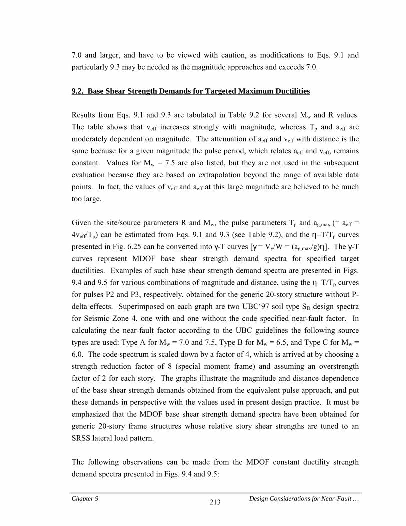
Chapter 9 Design Considerations for Near-Fault … 213
7.0 and larger, and have to be viewed with caution, as modifications to Eqs. 9.1 and particularly 9.3 may be needed as the magnitude approaches and exceeds 7.0. 9.2. Base Shear Strength Demands for Targeted Maximum Ductilities Results from Eqs. 9.1 and 9.3 are tabulated in Table 9.2 for several Mw and R values. The table shows that veff increases strongly with magnitude, whereas Tp and aeff are moderately dependent on magnitude. The attenuation of aeff and veff with distance is the same because for a given magnitude the pulse period, which relates aeff and veff, remains constant. Values for Mw = 7.5 are also listed, but they are not used in the subsequent evaluation because they are based on extrapolation beyond the range of available data points. In fact, the values of veff and aeff at this large magnitude are believed to be much too large. Given the site/source parameters R and Mw, the pulse parameters Tp and ag,max (= aeff = 4veff/Tp) can be estimated from Eqs. 9.1 and 9.3 (see Table 9.2), and the η–T/Tp curves presented in Fig. 6.25 can be converted into γ-T curves [γ== Vy/W = (ag,max/g)η]. The γ-T curves represent MDOF base shear strength demand spectra for specified target ductilities. Examples of such base shear strength demand spectra are presented in Figs. 9.4 and 9.5 for various combinations of magnitude and distance, using the η–T/Tp curves for pulses P2 and P3, respectively, obtained for the generic 20-story structure without P-delta effects. Superimposed on each graph are two UBC‘97 soil type SD design spectra for Seismic Zone 4, one with and one without the code specified near-fault factor. In calculating the near-fault factor according to the UBC guidelines the following source types are used: Type A for Mw = 7.0 and 7.5, Type B for Mw = 6.5, and Type C for Mw = 6.0. The code spectrum is scaled down by a factor of 4, which is arrived at by choosing a strength reduction factor of 8 (special moment frame) and assuming an overstrength factor of 2 for each story. The graphs illustrate the magnitude and distance dependence of the base shear strength demands obtained from the equivalent pulse approach, and put these demands in perspective with the values used in present design practice. It must be emphasized that the MDOF base shear strength demand spectra have been obtained for generic 20-story frame structures whose relative story shear strengths are tuned to an SRSS lateral load pattern. The following observations can be made from the MDOF constant ductility strength demand spectra presented in Figs. 9.4 and 9.5:
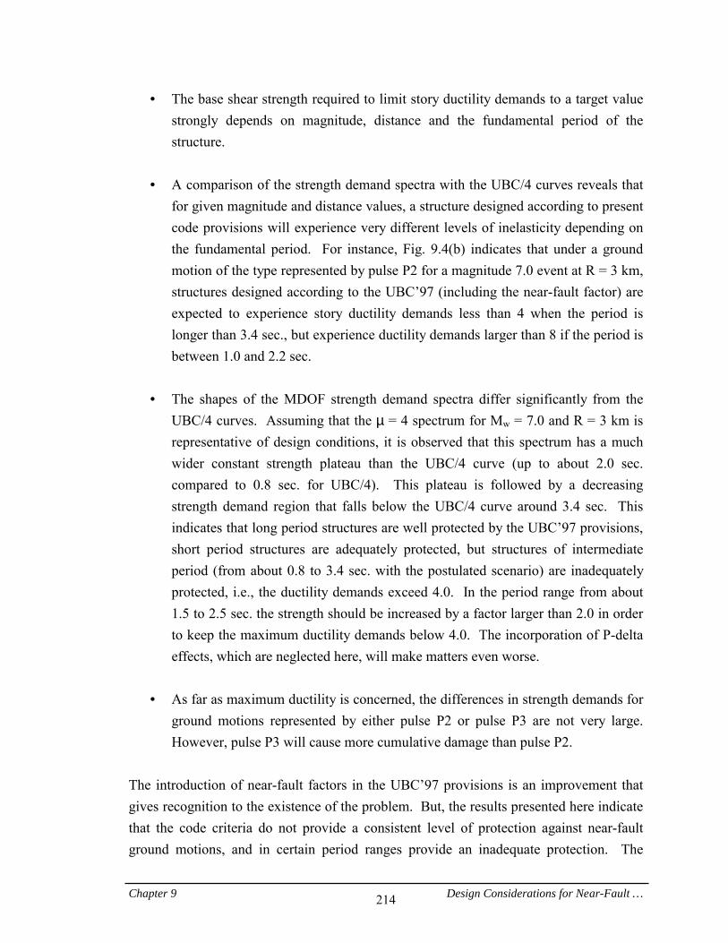
Chapter 9 Design Considerations for Near-Fault … 214
• = The base shear strength required to limit story ductility demands to a target value strongly depends on magnitude, distance and the fundamental period of the structure.
• = A comparison of the strength demand spectra with the UBC/4 curves reveals that
for given magnitude and distance values, a structure designed according to present code provisions will experience very different levels of inelasticity depending on the fundamental period. For instance, Fig. 9.4(b) indicates that under a ground motion of the type represented by pulse P2 for a magnitude 7.0 event at R = 3 km, structures designed according to the UBC’97 (including the near-fault factor) are expected to experience story ductility demands less than 4 when the period is longer than 3.4 sec., but experience ductility demands larger than 8 if the period is between 1.0 and 2.2 sec.
• = The shapes of the MDOF strength demand spectra differ significantly from the
UBC/4 curves. Assuming that the µ = 4 spectrum for Mw = 7.0 and R = 3 km is representative of design conditions, it is observed that this spectrum has a much wider constant strength plateau than the UBC/4 curve (up to about 2.0 sec. compared to 0.8 sec. for UBC/4). This plateau is followed by a decreasing strength demand region that falls below the UBC/4 curve around 3.4 sec. This indicates that long period structures are well protected by the UBC’97 provisions, short period structures are adequately protected, but structures of intermediate period (from about 0.8 to 3.4 sec. with the postulated scenario) are inadequately protected, i.e., the ductility demands exceed 4.0. In the period range from about 1.5 to 2.5 sec. the strength should be increased by a factor larger than 2.0 in order to keep the maximum ductility demands below 4.0. The incorporation of P-delta effects, which are neglected here, will make matters even worse.
• = As far as maximum ductility is concerned, the differences in strength demands for
ground motions represented by either pulse P2 or pulse P3 are not very large. However, pulse P3 will cause more cumulative damage than pulse P2.
The introduction of near-fault factors in the UBC’97 provisions is an improvement that gives recognition to the existence of the problem. But, the results presented here indicate that the code criteria do not provide a consistent level of protection against near-fault ground motions, and in certain period ranges provide an inadequate protection. The
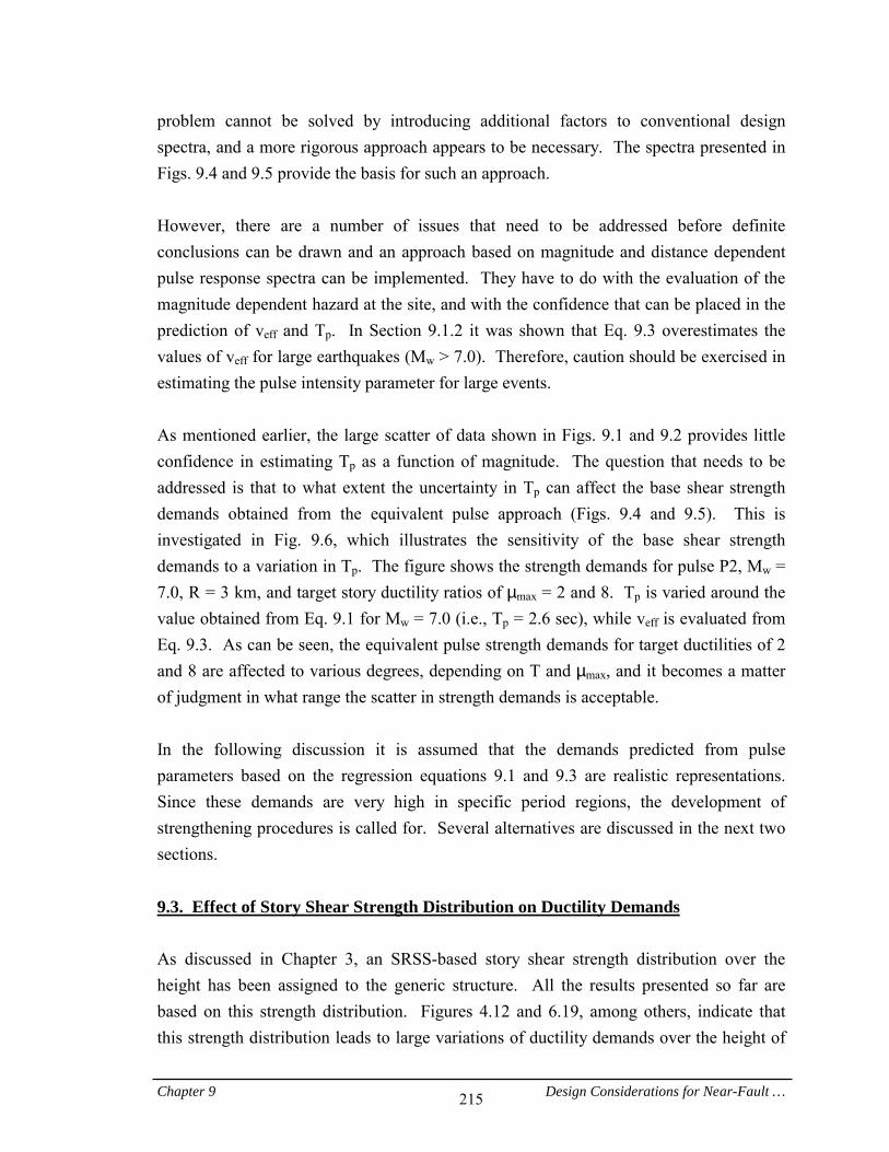
Chapter 9 Design Considerations for Near-Fault … 215
problem cannot be solved by introducing additional factors to conventional design spectra, and a more rigorous approach appears to be necessary. The spectra presented in Figs. 9.4 and 9.5 provide the basis for such an approach. However, there are a number of issues that need to be addressed before definite conclusions can be drawn and an approach based on magnitude and distance dependent pulse response spectra can be implemented. They have to do with the evaluation of the magnitude dependent hazard at the site, and with the confidence that can be placed in the prediction of veff and Tp. In Section 9.1.2 it was shown that Eq. 9.3 overestimates the values of veff for large earthquakes (Mw > 7.0). Therefore, caution should be exercised in estimating the pulse intensity parameter for large events. As mentioned earlier, the large scatter of data shown in Figs. 9.1 and 9.2 provides little confidence in estimating Tp as a function of magnitude. The question that needs to be addressed is that to what extent the uncertainty in Tp can affect the base shear strength demands obtained from the equivalent pulse approach (Figs. 9.4 and 9.5). This is investigated in Fig. 9.6, which illustrates the sensitivity of the base shear strength demands to a variation in Tp. The figure shows the strength demands for pulse P2, Mw = 7.0, R = 3 km, and target story ductility ratios of µmax = 2 and 8. Tp is varied around the value obtained from Eq. 9.1 for Mw = 7.0 (i.e., Tp = 2.6 sec), while veff is evaluated from Eq. 9.3. As can be seen, the equivalent pulse strength demands for target ductilities of 2 and 8 are affected to various degrees, depending on T and µmax, and it becomes a matter of judgment in what range the scatter in strength demands is acceptable. In the following discussion it is assumed that the demands predicted from pulse parameters based on the regression equations 9.1 and 9.3 are realistic representations. Since these demands are very high in specific period regions, the development of strengthening procedures is called for. Several alternatives are discussed in the next two sections. 9.3. Effect of Story Shear Strength Distribution on Ductility Demands As discussed in Chapter 3, an SRSS-based story shear strength distribution over the height has been assigned to the generic structure. All the results presented so far are based on this strength distribution. Figures 4.12 and 6.19, among others, indicate that this strength distribution leads to large variations of ductility demands over the height of
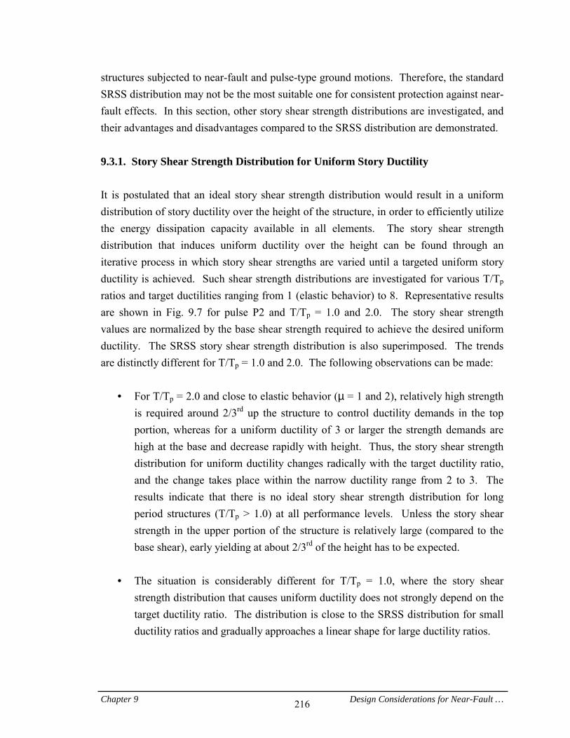
Chapter 9 Design Considerations for Near-Fault … 216
structures subjected to near-fault and pulse-type ground motions. Therefore, the standard SRSS distribution may not be the most suitable one for consistent protection against near-fault effects. In this section, other story shear strength distributions are investigated, and their advantages and disadvantages compared to the SRSS distribution are demonstrated. 9.3.1. Story Shear Strength Distribution for Uniform Story Ductility It is postulated that an ideal story shear strength distribution would result in a uniform distribution of story ductility over the height of the structure, in order to efficiently utilize the energy dissipation capacity available in all elements. The story shear strength distribution that induces uniform ductility over the height can be found through an iterative process in which story shear strengths are varied until a targeted uniform story ductility is achieved. Such shear strength distributions are investigated for various T/Tp ratios and target ductilities ranging from 1 (elastic behavior) to 8. Representative results are shown in Fig. 9.7 for pulse P2 and T/Tp = 1.0 and 2.0. The story shear strength values are normalized by the base shear strength required to achieve the desired uniform ductility. The SRSS story shear strength distribution is also superimposed. The trends are distinctly different for T/Tp = 1.0 and 2.0. The following observations can be made:
• = For T/Tp = 2.0 and close to elastic behavior (µ = 1 and 2), relatively high strength is required around 2/3rd up the structure to control ductility demands in the top portion, whereas for a uniform ductility of 3 or larger the strength demands are high at the base and decrease rapidly with height. Thus, the story shear strength distribution for uniform ductility changes radically with the target ductility ratio, and the change takes place within the narrow ductility range from 2 to 3. The results indicate that there is no ideal story shear strength distribution for long period structures (T/Tp > 1.0) at all performance levels. Unless the story shear strength in the upper portion of the structure is relatively large (compared to the base shear), early yielding at about 2/3rd of the height has to be expected.
• = The situation is considerably different for T/Tp = 1.0, where the story shear
strength distribution that causes uniform ductility does not strongly depend on the target ductility ratio. The distribution is close to the SRSS distribution for small ductility ratios and gradually approaches a linear shape for large ductility ratios.
Chapter 9 Design Considerations for Near-Fault … 217
The base shear strength required to limit the maximum story ductility to specific target values for pulse P2 and T/Tp = 2.0 and 1.0, respectively, is shown in Figs. 9.8(a) and (b). The normalized base shear strength is represented by the parameter η = Vy/(m.aeff). Results for two story shear strength distributions are shown: the solid line illustrates the base shear demands for the shear strength distribution that causes uniform story ductility, and the dotted line illustrates the base shear demands for the SRSS distribution. The following observations can be made:
• = For flexible structures (T/Tp = 2.0), the base shear strength demands strongly depend on the story shear strength distribution for a maximum story ductility of up to about 3.5, whereas for larger ductilities the demands are insensitive to the distribution of strength over the height. For these structures ductility control to a large extent is a function of both base shear strength and story shear strength distribution, except for relatively weak structures (µmax > 3.5) in which the first story is the critical one and the story shear strength distribution no longer matters.
• = The observations made for flexible structures do not apply to relatively stiff
structures (T/Tp = 1.0). The base shear strength required to limit the maximum ductility to a specific target value is not very sensitive to the selected story shear strength distribution, for all levels of ductility. The more important concern is the large η value required to limit the maximum story ductility to a reasonable value.
The conclusion is that no single story shear strength distribution will provide consistent protection at all performance levels and for structures with different periods. For long period structures either early damage in upper stories has to be tolerated (caused by ductility demands on the order of 3 to 4) or very high strength has to be provided over a large portion of the height. The strengthening of the lower portion of the structure will be very effective in reducing excessive ductility demands at the bottom. 9.3.2. Strengthening Schemes Based on Base Shear Strength and Story Shear Strength Distribution The results presented in the previous section demonstrate that the ductility demands in the upper portion of frame structures stabilize around 3 to 4, regardless of the story shear strength distribution employed in design. For weak structures (or very severe near-fault ground motions) the large demands usually occur in the bottom stories. Thus, in order to
Chapter 9 Design Considerations for Near-Fault … 218
prevent excessive ductility demands in severe events, it appears to be appropriate to strengthen the bottom portion of the structure compared to the standard SRSS story strength distribution. However, since such strengthening is associated with extra cost, cost effectiveness becomes an overriding issue, with the objective being to minimize the additional cost while providing adequate ductility control. This section summarizes several attempts to modify story shear strength distributions in a manner that will reduce the maximum story ductility demands while keeping down the cost of strengthening. Again, pulse P2 is assumed to represent near-fault ground motions. The following four story shear strength distributions, which are illustrated in Fig. 9.9, are investigated:
a) SRSS: the SRSS story shear strength distribution forming the baseline for this study, which is summarized in Section 3.2.2
b) SRSS + Strengthening: the SRSS distribution with the lower 30% of the structure strengthened with a linear strength increase leading to 40% extra strength at the base
c) Linear: a linear story shear strength distribution with a shear strength in the top story equal to 20% of the base shear
d) Linear + Strengthening: the linear distribution with a strengthened bottom portion defined in the same manner as in (b)
In all four cases the story stiffness is assumed to remain unchanged and is equal to that of the SRSS base case. The “SRSS + Strengthening” distribution requires extra steel weight compared to the base case, whereas the “Linear” distribution results in weight savings. If for simplicity it is assumed that weight is proportional to strength demand, the weight of the “Linear + Strengthening” distribution will be almost equal to that of the base case. The base shear strength for all four distributions is defined in terms of the parameter η = Vy/(m.aeff) of the SRSS base case without strengthening, i.e., the actual base shear of the cases with strengthening is defined by 1.4η. Since this η=is only a reference value for the strengthened frames, it is denoted as η* in Figs. 9.10 and 9.11. The story ductility demands for structures with T/Tp = 0.5, 1.0, and 2.0, and the four story strength distributions previously defined, are shown in Fig. 9.10. The graphs can be compared with the base case (Fig. 9.10(a)) to evaluate the benefits and shortcomings of each distribution. The following observations can be made:
Chapter 9 Design Considerations for Near-Fault … 219
• = For long period structures (T/Tp = 2.0) using the linear rather than SRSS strength distribution makes essentially no difference in the bottom stories, but causes somewhat larger ductility demands in the upper stories. Adding strength to the bottom portion of the structure does not much affect the ductility demands in the upper stories but has a significant benefit in the lower stories; the demands become more uniform over the bottom portion and the maximum ductility demand decreases by a factor that is in most cases larger than the strength increase factor of 1.4. (Since the story yield drift increases by the same factor as the story shear strength, the reduction in the story drift demands is smaller than that in the story ductility demands.) Thus, if the main objective is to protect the bottom stories from excessive ductility demands, then the use of a bilinear story shear strength distribution (Linear + Strengthening) appears to be very cost effective. The negative aspect is that the reduced strength in the upper stories will lead to earlier yielding in these stories compared to the base case. Better control of upper story ductility demands is achieved by using the SRSS + Strengthening distribution.
• = For short period structures (T/Tp = 0.5 and 1.0) the relative benefits are not well
established. Using the linear rather than SRSS strength distribution affects the ductility distribution over the height but has relatively little effect on the maximum story ductility demand. Providing additional strength in the bottom portion greatly reduces the ductility demand in the first story and leads to an upward shift of the critical story, but does not decrease the maximum demand significantly; for relatively strong structures, it even increases the demands compared to the unstrengthened structure. This applies particularly for structures with the linear strength distribution. Again, the use of the SRSS + Strengthening distribution appears to be a desirable compromise.
The conclusion is that strengthening of the bottom portion is an effective technique to control excessive ductility demands in the bottom stories, especially for flexible (T/Tp > 1.0) and relatively weak structures (or severe pulses), in which the migration of the critical story from the upper portion to the bottom story has occurred. The beneficial effects of this technique are limited to the strengthened stories and do not extend beyond.
Chapter 9 Design Considerations for Near-Fault … 220
P-Delta Effects: P-delta effects are usually largest in the first story, where the cumulative gravity load is maximum. Thus, there could be a considerable benefit in moving the maximum ductility demand away from the first story. The strengthening of the bottom portion, which moves the critical story upwards, is likely to decrease the P-delta effects considerably. This hypothesis is investigated in Fig. 9.11, which illustrates the distributions of story ductility demands in the presence of P-delta effects for structures with T/Tp = 0.5, 1.0, and 2.0, and story strengths distributed according to the (a) SRSS and (b) SRSS + Strengthening distributions. The following observations can be made:
• = For T/Tp = 2.0 and maximum ductility demands occurring in the bottom story, the strengthening of the bottom portion is even more beneficial than for the case of strengthening in the absence of P-delta effects. For relatively strong structures, in which the critical story is in the top portion, no beneficial effect is observed by adding strength to the bottom stories.
• = For T/Tp = 1.0 the strengthening scheme is again very effective in controlling high
ductility demands in the bottom story, but somewhat increases the maximum demand for strong structures.
• = As discussed in Section 6.2.2, P-delta effects are largest for short period structures
[provided that the stability coefficient of 0.1, which is used here to evaluate P-delta effects, applies to both long and short period structures]. This can also be observed from a comparison of Figs. 9.10(a) and 9.11(a) for T/Tp = 0.5. The results show that strengthening of the bottom stories is very effective in reducing the maximum ductility demand in short period structures at almost all performance levels – if the P-delta effect is significant.
The general conclusion is that in cases in which P-delta effects are significant, providing additional strength to the bottom portion of the structure is an efficient technique to control ductility demands for structures in all period ranges.
Chapter 9 Design Considerations for Near-Fault … 221
9.4. Strengthening of Frames with Walls The previous section provided information on frame strengthening schemes consisting of an increase in the base shear strength and modifications to the distribution of story shear strength over the height of the structure. As the results indicate, despite many successes, no single strengthening scheme can provide consistent improved protection of frames at all performance levels and for the full range of periods. As an alternative to those strengthening schemes, shear walls can be added to the frames to form a dual system. This section summarizes a study that investigates the demands for such dual systems subjected to pulse P2. The objective of this study is to evaluate the extent to which strengthening of frames with walls can improve the performance of structures in the near-fault region of an earthquake. In addition to conventional fixed-base walls, walls that can freely rotate about their bases are also studied. 9.4.1. Dual Systems Investigated in this Study The generic 20-story frame introduced in Section 3.2 is strengthened by adding a prismatic wall (constant cross-section over height of structure) that is either fixed or hinged at the base. Typical deflected shapes of these two dual systems are shown in Fig. 9.12. As illustrated, the wall is horizontally linked to the frame at story levels. The wall to frame stiffness ratio, Kw/Kf, is varied to investigate the effects of wall stiffness on the seismic demands of the system. The wall stiffness Kw is defined as the point load applied at the top of the wall corresponding to a unit displacement at the top, provided that the base is fixed and the wall behavior is elastic. If only prismatic walls are considered and shear deformations are neglected, Kw = 3EwIw/H3, where Ew, Iw, and H are the wall elastic modulus, moment of inertia, and height, respectively. Likewise, the frame stiffness Kf is defined as the point load at the roof level that causes a unit roof displacement. Elastic walls as well as inelastic walls with constant shear and bending strength over the height are considered. The base shear strength coefficient introduced in Chapter 6, i.e., ηf = Vframe,y/(m.ag,max), is used to define the frame strength. A similar strength coefficient, ηw = Vwall,y/(m.ag,max), is utilized to define the shear strength of the wall. Figure 9.13 shows base shear versus roof displacement diagrams obtained from pushover analyses of systems with (a) fixed and (b) hinged walls, in which the wall is assumed to
Chapter 9 Design Considerations for Near-Fault … 222
behave elastically. The SRSS lateral load pattern, to which the story stiffness and strength of the frame are tuned, is used in the pushover analyses. Adding a fixed wall to the frame increases the stiffness of the system significantly, and hence shortens the fundamental period of the system. The fundamental period of the so strengthened system, normalized by the period of the unstrengthened frame, is listed in Table 9.3 for various values of the Kw/Kf ratio. On the other hand, as the results of the pushover analysis indicate, if the wall is hinged at the base, it affects the stiffness of the system neither before nor after the formation of plastic hinges in the frame. The addition of a hinged wall also does not affect the pushover strength of the system. The reason is that the deflected shape of the frame subjected to the SRSS load pattern is a straight line (see Section 3.2), which corresponds to the rigid body motion of the hinged wall. Thus, regardless of wall stiffness, the stiffness of the system with the hinged wall does not change if the SRSS lateral load pattern is applied. The strength of the system also is unaffected because all plastic hinges in the frame form simultaneously under the SRSS lateral load pattern. It is also important to note that, since the first mode shape of the frame is close to a straight line, adding the hinged wall to the frame does not affect the first mode period of the system. 9.4.2. Demands for Dual Systems with Elastic Walls In this section, drift and force demands for systems with elastic fixed and hinged walls subjected to pulse P2 are evaluated. Both strong frames (low ductility demands) and weak frames (high ductility demands) with fundamental periods of T = 0.5 Tp, 1.0 Tp, and 2.0 Tp are considered. In each case the Kw/Kf ratio is varied within the range from 0.0 (no wall) to 2.0 (stiff wall) to study the effect of wall stiffness on the demands. Story Drift Demands: Figure 9.14 illustrates the effect of adding elastic fixed walls with various stiffnesses on the distribution of story drift demands for systems subjected to pulse P2. The story drift demands are normalized by the maximum ground displacement ug,max. Figure 9.15 shows corresponding results for systems strengthened with a wall that is hinged at the base. The drift demands for systems with strong (large η) and weak (small η) frames are presented side by side. Results for the unstrengthened system (Kw = 0) are shown in heavy solid lines, on which the maximum story ductility demand is indicated. For the systems with fixed walls, the period T corresponds to the frame alone. As explained earlier, the
Chapter 9 Design Considerations for Near-Fault … 223
fundamental period of the strengthened system is considerably shortened by adding a fixed wall. The following observations can be made from Figs. 9.14 and 9.15:
• = Fixed walls are very effective in reducing the drift demands for structures with T/Tp < 1.0, but become much less effective in reducing the demands for T/Tp ≥ 1.0. In some cases the addition of a fixed wall even increases the maximum drift demand. The reason for the latter is higher mode effects as well as the fact that for T/Tp > 0.75 the elastic strength demand spectrum of pulse P2 is descending, and thus the period shortening of the system due to strengthening with a fixed wall leads to a rapid increase in base shear demands.
• = Hinged walls are effective in reducing the drift demands for frames with T/Tp
both smaller and larger than 1.0. For systems with T/Tp = 0.5 the reduction is significant for weak systems and can be accomplished with relatively flexible walls. Similar observations also hold true for systems with T/Tp = 1.0. The effectiveness of adding hinged walls is largest for T/Tp = 2.0, where walls significantly reduce the large drift demands in the upper portion of strong structures and in the bottom stories of weak structures. However, relatively stiff walls are needed to accomplish significant drift reduction in the case of weak frames with high ductility demands at the base.
• = In a system strengthened with a hinged wall, three components contribute to the
horizontal displacement of the wall: 1) bending deformations, 2) shear deformations, and 3) rotation about the base. If the wall is stiff compared to the frame, bending and shear deformations will become small and a rigid body rotation will dominate the wall displacement, resulting in a close to uniform distribution of drift demands over the height. Shear deformations are ignored here, but their effects will be studied later in this section.
• = The wall stiffness (relative to frame stiffness) needed for effective drift control
increases with the T/Tp ratio. For strengthening with a hinged wall, minimum required Kw/Kf values for effective drift control are deduced to be 0.25, 0.5, and 2.0 (a value as low as 1.0 could have been chosen) for T/Tp ratios of 0.5, 1.0, and 2.0, respectively. Hence, considering that the frame stiffness is proportional to 1/T2, for a given Tp value, the absolute wall stiffness (Kw) values for T/Tp = 0.5, 1.0, and 2.0 will be proportional to 1.0:0.5:0.5.
Chapter 9 Design Considerations for Near-Fault … 224
• = For all three weak frames (with different T/Tp) strengthened with stiff hinged walls, the drift demand is almost the same (about 0.06 ug,max) regardless of the frame period. The reason is that when the hinged wall is stiff compared to the frame, the dual system acts as an SDOF oscillator, whose only mode of vibration is a straight line. As shown in Fig. 6.31, the inelastic displacement demand of weak SDOF systems is almost independent of the T/Tp ratio because a weak system yields rapidly resulting in a large reduction of the stiffness. The displacement demand for systems with small stiffness is close to the peak ground displacement and has little to do with the initial elastic period.
Wall Shear and Moment Demands: From the study of drift demands it appears that for a given wall stiffness, elastic fixed walls are more effective in reducing drift demands for short period frames (T/Tp < 1.0), while elastic hinged walls are more effective for long period frames (T/Tp > 1.0). However, these results do not address force (shear and moment) demands imposed on the wall. The force demands will determine the feasibility of making the walls sufficiently strong to justify the assumption of elastic wall behavior. Figures 9.16 and 9.17 illustrate elastic shear strength demands for fixed and hinged walls of different stiffness used to strengthen frames of various periods and strength subjected to pulse P2. The results are organized in the same manner as in Figs. 9.14 and 9.15. The wall shear demands are normalized by m.ag,max, where m is the total mass of the structure, and ag,max is the maximum ground acceleration of the pulse. Similarly, elastic moment demands for the fixed and hinged walls are illustrated in Figs. 9.18 and 9.19. The wall moment demands are normalized by H.m.ag,max, where H is the total height of the structure. The following observations can be made from these figures:
• = For the stiff fixed walls the shear strength demands become very large in the bottom stories regardless of frame strength and T/Tp. These demands are much larger than those for the elastic hinged walls. This is in part because of the period shift that occurs by adding a fixed shear wall to the system.
• = When a fixed wall is used for strengthening, the shear demands increase rather
consistently with the stiffness of the wall for T/Tp ≥ 1.0, whereas this pattern is not observed consistently for T/Tp = 0.5. This aberration can be rationalized by large and frequent peaks and valleys in the elastic strength demand spectrum of
Chapter 9 Design Considerations for Near-Fault … 225
pulse P2 for T/Tp < 0.5, which is the period range that contains the shifted fundamental period of the strengthened system.
• = Even though there is only a negligible shift of the fundamental period caused by
adding a hinged wall, a similar aberration is also observed in the hinged wall case, i.e., the shear demand does not necessarily increase with wall stiffness. The reason is that while the first mode period of the system remains unchanged, adding a hinged wall to the system affects its higher mode periods, shortening them significantly. If the shifted higher mode periods – especially the second mode – coincide with one of the large peaks of the elastic strength spectrum, higher mode effects become more significant, resulting in a larger shear demand for the strengthened system.
• = The distributions and values of the shear demands over the height for hinged
walls are similar, regardless of T/Tp and frame strength. This provides a great advantage in design, considering the large uncertainties in predicting the period of the equivalent pulse (see Section 9.1.1). The maximum base shear strength demand in almost all cases studied here is about 0.6m.ag,max. The demands show little sensitivity to wall stiffness for T/Tp = 0.5, but this sensitivity increases for longer periods.
• = The wall moment demands for the hinged walls are merely a small fraction of the
demands for the fixed wall. While the moment demands for the fixed walls consistently increase from top to bottom, the maximum demands for the hinged walls occur at around 40% of the height and do not exceed 0.16H.m.ag,max by much.
In the results presented so far, both weak and strong frames were considered in order to explore the effects of adding walls to frames of different strength. However, for the purpose of practicality, frame strength should be looked at in the context of realistic design requirements. Assuming that the frame is designed for an event with Mw = 7.0 and R = 3 km, the period and intensity of the equivalent pulse are estimated from Eqs. 9.1 and 9.3, i.e., Tp = 2.6 sec. and ag,max = 4veff/Tp = 0.31g. Then, considering a strength reduction factor of 8 and an overstrength factor of 2, the base shear strength (γ = Vy/W) of the frame is obtained from the UBC design spectrum with the near-fault factor for Mw = 7.0 and R = 3 km (see Fig. 9.4). For T/Tp = 0.5, 1.0 and 2.0 [or T = (0.5)(2.6) = 1.3,
Chapter 9 Design Considerations for Near-Fault … 226
2.6, and 5.2 sec.] the so obtained strength coefficient γ is 0.23, 0.15, and 0.15, respectively. Finally, the base shear strength coefficient, η, is computed from the equation η = γ/(ag,max/g), i.e., η = 0.74, 0.48, and 0.48. In the remainder of this chapter, for each of the three T/Tp values, results are presented only for the frame whose base shear strength coefficient is closer to these η values (i.e., η = 0.75, 0.2, and 0.5, for T/Tp = 0.5, 1.0, and 2.0, respectively). Effect of Shear Deformations: The effects of wall shear deformations on drift demands have been ignored so far. Typically, shear deformations contribute significantly to the total deformation if the wall M/V ratio is small and the wall is stocky. For the hinged walls the M/V ratio is approximately (0.16.H.m.ag,max)/(0.6.m.ag,max) ≅ 0.25H, which indeed is small. Figure 9.20 illustrates distributions of story drift demands, incorporating the effects of shear deformations, for frames strengthened with (a) fixed and (b) hinged walls with aspect ratios (b/H) ranging from 0.0 (no shear deformations) to 0.5 (stocky wall). In each case a (Kw/Kf) value is chosen that corresponds to the minimum hinged wall stiffness required to achieve a relatively uniform distribution of drift over the height in the absence of shear deformations. A rectangular wall cross-section and a Poisson’s ratio of ν = 0.17 are considered in computing the shear deformations. The following observations can be made:
• = For the fixed walls the effects of shear deformations are small in the top portion and large in the bottom portion of the wall. Nevertheless, the drift demands at the bottom of the structure are still much smaller than the demands at the top, and are not a matter of concern.
• = For the hinged walls the effects of shear deformations are relatively small
everywhere, even for stocky walls. The small shear deformation effects may come as a surprise especially in the lower portion of the wall, where shear demands are large and moment demands are very small. However, it should be noted that these results are obtained for walls in which rotation about the base dominates over flexural and shear modes of deformation.
The general conclusion is that it is acceptable to neglect the effects of wall shear deformations on drift demands for frames strengthened with hinged walls.

Chapter 9 Design Considerations for Near-Fault … 227
P-Delta Effects: To illustrate the beneficial effects of strengthening in the presence of P-delta effects, Fig. 9.21 shows distributions of story drift demands over the height for systems strengthened with (a) fixed and (b) hinged walls when P-delta effects are taken into account. The heavy solid lines represent the distribution for unstrengthened frames with the gravity loads introduced in Section 3.2.3. The same gravity loads are used for strengthened frames to trigger P-delta effects. The following observations can be made:
• = As discussed in Section 6.2.2, P-delta effects typically increase maximum story ductility (or drift) demands for unstrengthened frames. However, a comparison of the drift distribution for T/Tp = 0.5 in Fig. 9.21 with the corresponding distribution in Fig. 9.14 indicates that for a frame with T/Tp = 0.5 and η = 0.75 the maximum drift is smaller in the presence of P-delta effects. This aberration, which appears as a sharp kink in the η-µmax curve shown in Fig. 6.21(b) for P2, is limited to short period frames in a narrow range of strength, and can be explained by period shifts due to P-delta effects in a very sensitive region of the elastic spectrum of pulse P2. Nonetheless, adding a fixed wall reduces the maximum demand effectively. Strengthening with a hinged wall is also beneficial, although to a lesser degree.
• = For T/Tp = 1.0 and η = 0.2, a comparison shows that P-delta effects lead to a
considerable increase in maximum story drift demands for unstrengthened frames. While adding a fixed wall may not be effective in reducing the drifts in the top stories, strengthening with a hinged wall proves to be very effective.
• = For T/Tp = 2.0 and η = 0.5, P-delta effects for the unstrengthened frame are not
large because the maximum story drift does not occur in the bottom story, where gravity loads are largest. Nevertheless, similar to the case without P-delta effects, adding hinged walls effectively reduces the maximum drift demands.
The conclusion from these results is that strengthening frames with walls reduces story drift demands of frame structures, especially excessive demands in bottom stories, and therefore can provide improved protection against P-delta effects.
Chapter 9 Design Considerations for Near-Fault … 228
9.4.3. Demands for Inelastic Walls From the results presented so far, it appears that strengthening with a wall hinged at the base is an attractive technique for reducing the drift demands of frame structures subjected to pulse-type ground motions. However, the results have been obtained under the assumption that the wall behaves elastically, which may be difficult to achieve when the shear or moment demands of the wall become large. The formation of plastic regions in fixed walls is almost inevitable during a major event. If a fixed wall is designed carefully, a brittle shear failure, to which a reinforced concrete wall is most susceptible, can be prevented. However, shear yielding in the bottom portion of a hinged wall, where shear demands are large and moment demands are small, may not be avoidable. In this section demands for systems with inelastic fixed and hinged walls subjected to pulse P2 are investigated. Flexural yielding in fixed walls and shear yielding in hinged walls are studied to assess the effects of wall inelastic behavior on the benefits of strengthening, highlighted previously for elastic walls. Three frames with fundamental periods of T = 0.5 Tp, 1.0 Tp, and 2.0 Tp and base shear strength coefficients of ηf = 0.75, 0.2, and 0.5 are considered. For each T/Tp the smallest Kw/Kf ratio is chosen that can provide a relatively uniform distribution of drift over the height based on the results presented in the previous section for elastic hinged walls. For comparison purposes, the same Kw/Kf values also are used for the fixed walls. Hinged Walls: Figure 9.22 illustrates distributions of various demands over the height for systems strengthened with hinged walls. The plots serve to compare demands for systems with elastic and inelastic walls. The heavy solid line in Fig. 9.22(a) represents story drift demands for unstrengthened frames. The inelastic walls can yield in shear in any story in which the shear demand reaches the shear capacity, which is assumed to be constant over the height. The wall shear capacity is varied using the shear strength parameter ηw = Vwall,y/(m.ag,max), which is denoted as “eta(w)” in the figure. A bilinear hysteretic story shear-drift relationship is used with no strain hardening. Wall elastic shear stiffness is determined assuming a rectangular cross-section, an aspect ratio (b/H) of 0.25, and a Poisson’s ratio of 0.17. The following observations can be made:
Chapter 9 Design Considerations for Near-Fault … 229
• = As Fig. 9.22(a) indicates, shear yielding of the wall does not cause a significant increase in the total story drifts of the system (for T/Tp = 1.0 it even decreases the demands). A comparison with the demands for the unstrengthened frame shows that adding a hinged wall with limited shear strength can still effectively reduce the drift demands of the frame and provide improved protection.
• = Figure 9.22(b) shows that the wall shear drift demands (contribution of wall shear
deformations to drift) for elastic walls are negligible (compared to the total drifts), but the demands increase rapidly in the bottom portion of the wall when shear yielding occurs. Of all the cases studied here, the wall shear drift demand is largest for T/Tp = 2.0, ηf = 0.5, and ηw = 0.2, i.e., δshear = 0.047ug,max. Using Eqs. 9.1 and 9.3 for a scenario event with Mw = 7 and R = 3 km, and considering the relationship ug,max = vg,maxTp/4 for pulse P2, the peak ground displacement can be estimated as ug,max = 51 in. Thus, the drift angle due to wall shear deformations is computed to be δshear/h = (0.047)(51)/(144) = 0.017, where h is the story height. This drift angle is large, but later in this section it will be shown that ηw = 0.2 corresponds to a low shear strength capacity of the wall, and hence the shear drift demands will be smaller than the value calculated here.
• = Figure 9.22(c) demonstrates that for very weak walls, the top portion of the wall
may also yield in shear. However, unlike the bottom, the shear yielding at the top is not associated with large inelastic shear deformations in the wall.
• = Figure 9.22(d) shows that the shear yielding of the wall consistently reduces the
wall moment demands. This pilot study indicates that some shear yielding in hinged walls used to strengthen frames against near-fault ground motions has to be expected. Some shear yielding should be acceptable for reinforced concrete walls, particularly if the axial force in the wall is kept low. Steel shear walls may provide an effective alternative that can accommodate large inelastic shear deformations. Fixed Walls: It is assumed that the fixed walls can only yield in bending with no shear plastification. Thus, wall shear deformations are neglected as with the elastic walls in the preceding
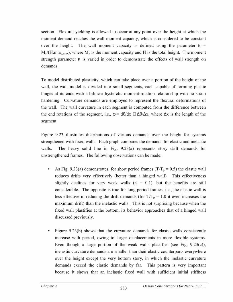
Chapter 9 Design Considerations for Near-Fault … 230
section. Flexural yielding is allowed to occur at any point over the height at which the moment demand reaches the wall moment capacity, which is considered to be constant over the height. The wall moment capacity is defined using the parameter κ = My/(H.m.ag,max), where My is the moment capacity and H is the total height. The moment strength parameter κ is varied in order to demonstrate the effects of wall strength on demands. To model distributed plasticity, which can take place over a portion of the height of the wall, the wall model is divided into small segments, each capable of forming plastic hinges at its ends with a bilinear hysteretic moment-rotation relationship with no strain hardening. Curvature demands are employed to represent the flexural deformations of the wall. The wall curvature in each segment is computed from the difference between the end rotations of the segment, i.e., φ = dθ/dx ≅ ∆θ/∆x, where ∆x is the length of the segment. Figure 9.23 illustrates distributions of various demands over the height for systems strengthened with fixed walls. Each graph compares the demands for elastic and inelastic walls. The heavy solid line in Fig. 9.23(a) represents story drift demands for unstrengthened frames. The following observations can be made:
• = As Fig. 9.23(a) demonstrates, for short period frames (T/Tp = 0.5) the elastic wall reduces drifts very effectively (better than a hinged wall). This effectiveness slightly declines for very weak walls (κ = 0.1), but the benefits are still considerable. The opposite is true for long period frames, i.e., the elastic wall is less effective in reducing the drift demands (for T/Tp = 1.0 it even increases the maximum drift) than the inelastic walls. This is not surprising because when the fixed wall plastifies at the bottom, its behavior approaches that of a hinged wall discussed previously.
• = Figure 9.23(b) shows that the curvature demands for elastic walls consistently
increase with period, owing to larger displacements in more flexible systems. Even though a large portion of the weak walls plastifies (see Fig. 9.23(c)), inelastic curvature demands are smaller than their elastic counterparts everywhere over the height except the very bottom story, in which the inelastic curvature demands exceed the elastic demands by far. This pattern is very important because it shows that an inelastic fixed wall with sufficient initial stiffness

Chapter 9 Design Considerations for Near-Fault … 231
deflects roughly as a straight line over most of its height and only bends at the very bottom considerably. This concentration of rotation at the base indicates that weak fixed walls behave in a similar manner as hinged walls, and therefore can reduce drift demands effectively, provided that shear failure at the base is prevented.
• = Figure 9.23(c) indicates that in flexible frames (T/Tp = 1.0 and 2.0), for which the
elastic wall moment demands are large, a reduction of the wall bending strength will lead to plastification that is not limited to a small zone near the base but spreads over a large portion of the height. For the weakest wall studied here, i.e. κ = 0.1, the plastified zone comprises the entire bottom half of the structure. On the other hand, in stronger walls (κ = 0.4), only a small portion of the wall adjacent to the base plastifies.
• = Figure 9.23(d) shows that plastification of the wall due to flexural yielding
consistently reduces the wall shear demands. This reduction is larger for more flexible systems, in which flexural yielding extends over a larger portion of the wall. However, the bad news is that the reduced shear demands are still as high as, or higher than, the shear demands for the elastic hinged wall. Thus, it will be very difficult to provide sufficient shear resistance to avoid undesirable shear yielding in conjunction with flexural yielding.
The conclusion is that strengthening with hinged walls that yield in shear is still beneficial in reducing story drift demands, and that strengthening with fixed walls that yield in flexure will lead to a concentration of large plastic rotations in the bottom story. As the wall moment strength capacity decreases, the behavior of the fixed wall approaches that of a hinged wall. It will be difficult in such cases to provide the shear resistance necessary to avoid shear yielding. Thus, strengthening with hinged walls appears to be a more effective technique. Use of Reinforced Concrete Walls for Strengthening: The values used in the previous discussion for the wall shear and flexural strength parameters (ηw and κ) need to be put in perspective. The following example serves to provide reasonable estimates for the shear and moment strength capacity of a reinforced concrete shear wall that can effectively strengthen frames subjected to pulse-type ground
Chapter 9 Design Considerations for Near-Fault … 232
motions. The wall cross-section is assumed to be rectangular with a width of lw = 360 in. and an unknown thickness of t. The results of a modal analysis for the generic 20-story frame used in this study indicate that the stiffness (Kf [kip/in]), as defined in Section 9.4.1, total seismic mass (m [kip.sec2/in]), and period (T [sec]) of the structure are related as follows:
2f Tm 12.50 K = (9.5)
As discussed in Section 9.4.2, a desirable wall stiffness for T/Tp = 0.5, 1.0, and 2.0 is Kw = 0.25 Kf, 0.5 Kf, and 2.0 Kf, respectively. Substituting for Kf from Eq. 9.5, and using the equation for wall flexural stiffness, i.e. Kw = 3EwIw/Hw
3 (Ew is modulus of elasticity, Iw is moment of inertia, and Hw is total height), values for a desirable Iw can be determined for the three T/Tp cases. For T/Tp = 0.5 the result is:
2w
3w
w TEmH
1.04 I = (9.6)
Continuing the illustrative example for T/Tp = 0.5, for a scenario event with Mw = 7 and R = 3 km, the pulse parameters are Tp = 2.6 sec. and ag,max = 0.31g, and hence T = 1.3 sec. The total frame height for a 20-story building is Hw = 2880 in. The modulus of elasticity for reinforced concrete can be estimated from the ACI equation (f’
c = 4000 psi) as follows:
ksi3605f 57 E 'cw == (9.7)
Substituting for T, Hw, and Ew in Eq. 9.6, the desirable wall moment of inertia, in terms of the mass m, is found to be Iw = 4.08×10⁶m. For a rectangular section with lw = 360 in., the required thickness can be computed as t = 12Iw/lw
3 = 1.05m. Similar calculations for T/Tp = 1.0 and 2.0 results in t = 0.53m for both cases. These wall thickness-mass relationships can be used to estimate the wall shear strength capacity as follows: According to ACI 318-99, the wall shear strength provided by the concrete for aspect ratios Hw/lw ≥ 2.0 can be estimated as:

Chapter 9 Design Considerations for Near-Fault … 233
46t1000
(360)t4,0002Af2V cv
'cc === (9.8)
If minimum shear reinforcement (ρn = 0.0025) with fy = 60,000 psi is used, the shear strength provided by the reinforcement is:
54t1000
0)025)(60,00(360)t(0.0fρAV yncvs === (9.9)
Therefore, the total minimum shear strength of the wall is Vn = Vc + Vs = 100t. Using the t-m relationships found above and normalizing the shear strength by m.ag,max, where ag,max = 0.31g for the scenario event under consideration, ηw = Vn/(m.ag,max) = 0.88, 0.44, and 0.44 for T/Tp = 0.5, 1.0, and 2.0, respectively. As shown in Fig. 9.17, the maximum base shear strength demand for elastic hinged walls in almost all cases is about 0.6m.ag,max, which is only slightly larger than the values estimated for the minimum shear capacity of the reinforced concrete wall used in the example. Considering that adding more reinforcement will further increase the shear strength capacity, it appears that shear yielding, which may result in a brittle mode of failure in reinforced concrete walls, can be prevented. This conclusion supports the use of hinged reinforced concrete walls as a beneficial strengthening technique. To estimate the bending strength capacity of the example wall, boundary zones are considered to be fully imbedded in the wall, each 40 in. wide. As an example, the reinforcement ratio in each boundary zone is assumed to be 3%, amounting to As = 0.03(40)t = 1.2t. For this case the nominal bending strength is conservatively estimated as Mn = 24,000t. After substituting for t from the t-m relationships and normalizing by m.H.ag,max, the normalized moment capacity for T/Tp = 0.5, 1.0, and 2.0 is computed as κ = Mn/(m.H.ag,max) = 0.07, 0.04, and 0.04. These estimates are much smaller than the elastic moment demands for fixed walls. They are even smaller than the moment demands for elastic hinged walls. Thus, under the assumptions made in this example, it appears that avoiding flexural yielding in the wall may be difficult (but not impossible for hinged walls) and requires heavy flexural reinforcement. If the hinged wall yields in bending, as the previous example suggested, the effectiveness of the wall in reducing the maximum story drift demand needs to be reevaluated. This reevaluation is illustrated in Fig. 9.24, which shows distributions of story drift and wall
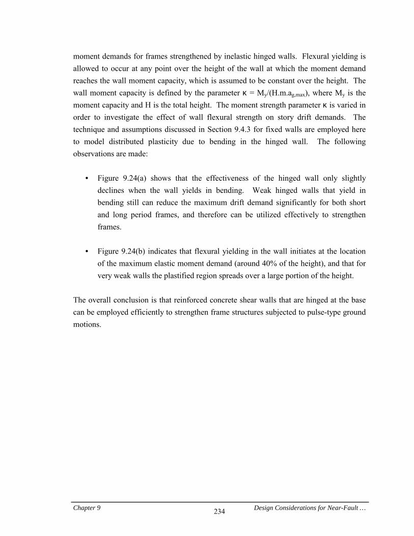
Chapter 9 Design Considerations for Near-Fault … 234
moment demands for frames strengthened by inelastic hinged walls. Flexural yielding is allowed to occur at any point over the height of the wall at which the moment demand reaches the wall moment capacity, which is assumed to be constant over the height. The wall moment capacity is defined by the parameter κ = My/(H.m.ag,max), where My is the moment capacity and H is the total height. The moment strength parameter κ is varied in order to investigate the effect of wall flexural strength on story drift demands. The technique and assumptions discussed in Section 9.4.3 for fixed walls are employed here to model distributed plasticity due to bending in the hinged wall. The following observations are made:
• = Figure 9.24(a) shows that the effectiveness of the hinged wall only slightly declines when the wall yields in bending. Weak hinged walls that yield in bending still can reduce the maximum drift demand significantly for both short and long period frames, and therefore can be utilized effectively to strengthen frames.
• = Figure 9.24(b) indicates that flexural yielding in the wall initiates at the location
of the maximum elastic moment demand (around 40% of the height), and that for very weak walls the plastified region spreads over a large portion of the height.
The overall conclusion is that reinforced concrete shear walls that are hinged at the base can be employed efficiently to strengthen frame structures subjected to pulse-type ground motions.
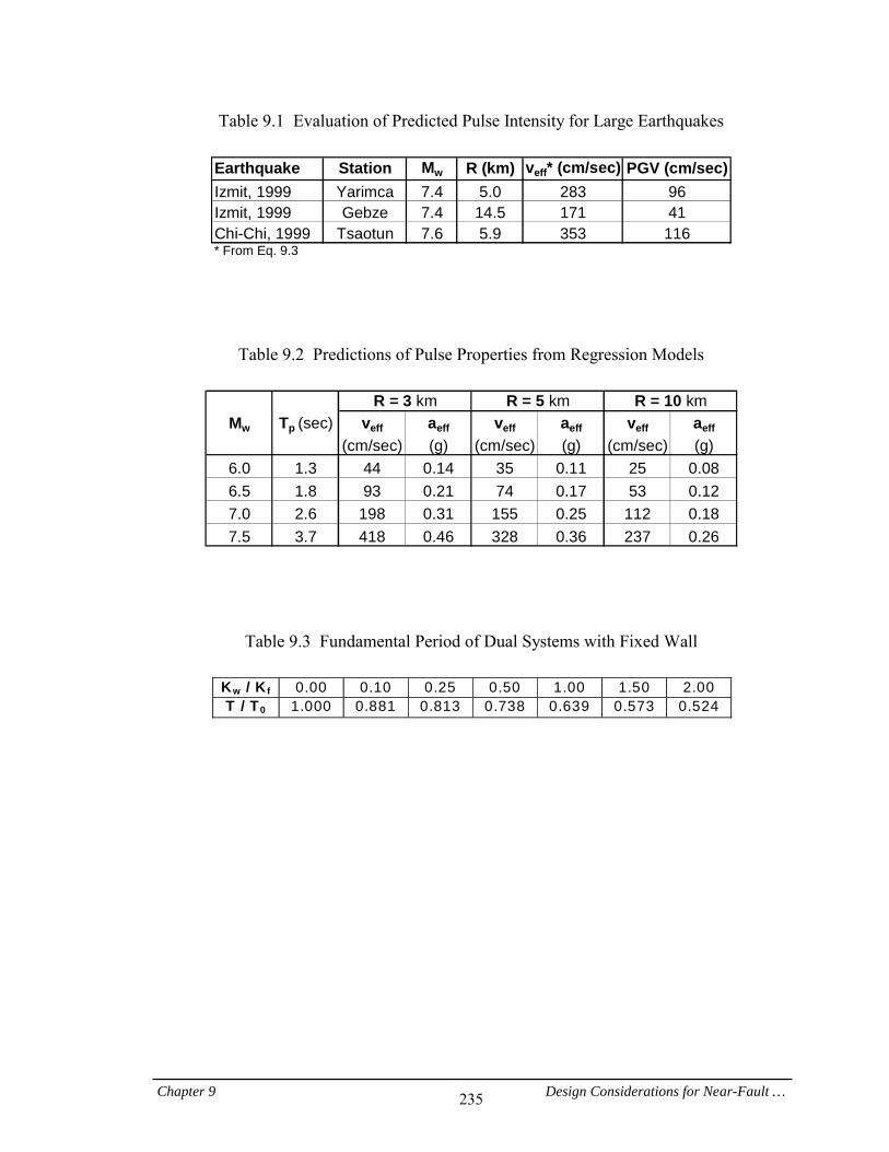
Chapter 9 Design Considerations for Near-Fault … 235
Table 9.1 Evaluation of Predicted Pulse Intensity for Large Earthquakes
Earthquake Station Mw R (km) veff* (cm/sec) PGV (cm/sec)Izmit, 1999 Yarimca 7.4 5.0 283 96Izmit, 1999 Gebze 7.4 14.5 171 41Chi-Chi, 1999 Tsaotun 7.6 5.9 353 116* From Eq. 9.3
Table 9.2 Predictions of Pulse Properties from Regression Models
Mw Tp (sec) veff aeff veff aeff veff aeff
(cm/sec) (g) (cm/sec) (g) (cm/sec) (g)6.0 1.3 44 0.14 35 0.11 25 0.086.5 1.8 93 0.21 74 0.17 53 0.127.0 2.6 198 0.31 155 0.25 112 0.187.5 3.7 418 0.46 328 0.36 237 0.26
R = 3 km R = 5 km R = 10 km
Table 9.3 Fundamental Period of Dual Systems with Fixed Wall
Kw / Kf 0.00 0.10 0.25 0.50 1.00 1.50 2.00 T / T0 1.000 0.881 0.813 0.738 0.639 0.573 0.524
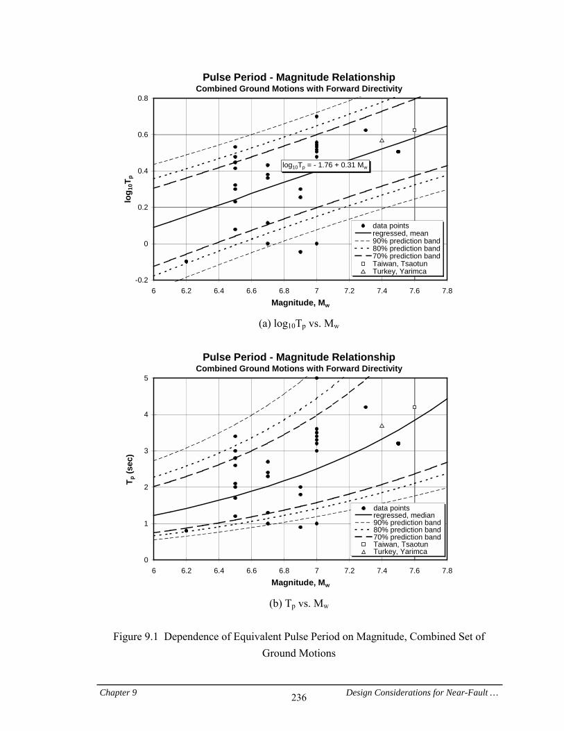
Chapter 9 Design Considerations for Near-Fault … 236
Pulse Period - Magnitude RelationshipCombined Ground Motions with Forward Directivity
-0.2
0
0.2
0.4
0.6
0.8
6 6.2 6.4 6.6 6.8 7 7.2 7.4 7.6 7.8Magnitude, Mw
log 1
0Tp
data pointsregressed, mean90% prediction band80% prediction band70% prediction bandTaiwan, TsaotunTurkey, Yarimca
log10Tp = - 1.76 + 0.31 Mw
(a) log10Tp vs. Mw
Pulse Period - Magnitude Relationship
Combined Ground Motions with Forward Directivity
0
1
2
3
4
5
6 6.2 6.4 6.6 6.8 7 7.2 7.4 7.6 7.8Magnitude, Mw
T p (s
ec)
data pointsregressed, median90% prediction band80% prediction band70% prediction bandTaiwan, TsaotunTurkey, Yarimca
(b) Tp vs. Mw
Figure 9.1 Dependence of Equivalent Pulse Period on Magnitude, Combined Set of
Ground Motions
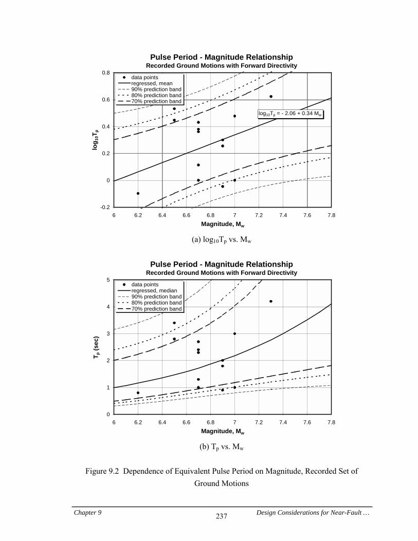
Chapter 9 Design Considerations for Near-Fault … 237
Pulse Period - Magnitude RelationshipRecorded Ground Motions with Forward Directivity
-0.2
0
0.2
0.4
0.6
0.8
6 6.2 6.4 6.6 6.8 7 7.2 7.4 7.6 7.8Magnitude, Mw
log 1
0Tp
data pointsregressed, mean90% prediction band80% prediction band70% prediction band
log10Tp = - 2.06 + 0.34 Mw
(a) log10Tp vs. Mw
Pulse Period - Magnitude Relationship
Recorded Ground Motions with Forward Directivity
0
1
2
3
4
5
6 6.2 6.4 6.6 6.8 7 7.2 7.4 7.6 7.8Magnitude, Mw
T p (s
ec)
data pointsregressed, median90% prediction band80% prediction band70% prediction band
(b) Tp vs. Mw
Figure 9.2 Dependence of Equivalent Pulse Period on Magnitude, Recorded Set of
Ground Motions
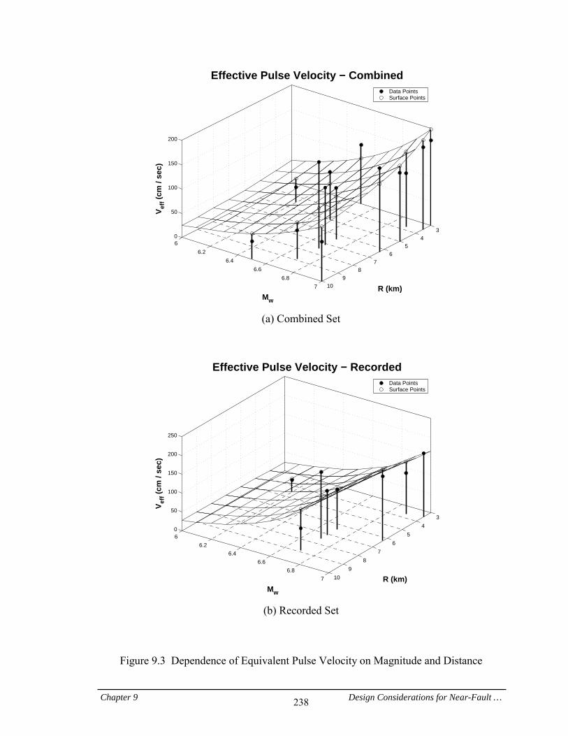
Chapter 9 Design Considerations for Near-Fault … 238
34
56
78
910
6
6.2
6.4
6.6
6.8
7
0
50
100
150
200
R (km)
Effective Pulse Velocity − Combined
Mw
Vef
f (cm
/ se
c)
Data Points Surface Points
(a) Combined Set
3
4
5
6
7
8
9
10
6
6.2
6.4
6.6
6.8
7
0
50
100
150
200
250
R (km)
Effective Pulse Velocity − Recorded
Mw
Vef
f (cm
/ se
c)
Data Points Surface Points
(b) Recorded Set
Figure 9.3 Dependence of Equivalent Pulse Velocity on Magnitude and Distance
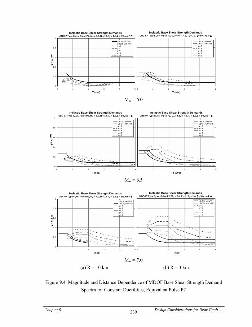
Chapter 9 Design Considerations for Near-Fault … 239
Inelastic Base Shear Strength DemandsUBC-97 Type SD vs. Pulse P2, Mw = 6.0, R = 10, Tp = 1.3, ξξξξ = 5%, no P-∆∆∆∆
0
0.2
0.4
0.6
0.8
1
0 1 2 3 4 5
T (sec)
γγ γγ =
V y /
W
UBC/4, no NFFUBC/4, with NFFµ===2µ===3µ===4µ===6µ===8
Inelastic Base Shear Strength DemandsUBC-97 Type SD vs. Pulse P2, Mw= 6.0, R = 3, Tp = 1.3, ξξξξ = 5%, no P-∆∆∆∆
0 1 2 3 4 5
T (sec)
UBC/4, no NFFUBC/4, with NFFµ===2µ===3µ===4µ===6µ===8
Mw = 6.0
Inelastic Base Shear Strength Demands
UBC-97 Type SD vs. Pulse P2, Mw = 6.5, R = 10, Tp = 1.8, ξξξξ = 5%, no P-∆∆∆∆
0
0.2
0.4
0.6
0.8
1
0 1 2 3 4 5
T (sec)
γγ γγ =
V y /
W
UBC/4, no NFFUBC/4, with NFFµ===2µ===3µ===4µ===6µ===8
Inelastic Base Shear Strength DemandsUBC-97 Type SD vs. Pulse P2, Mw = 6.5, R = 3, Tp = 1.8, ξξξξ = 5%, no P-∆∆∆∆
0 1 2 3 4 5
T (sec)
UBC/4, no NFFUBC/4, with NFFµ===2µ===3µ===4µ===6µ===8
Mw = 6.5
Inelastic Base Shear Strength Demands
UBC-97 Type SD vs. Pulse P2, Mw = 7.0, R = 10, Tp = 2.6, ξξξξ = 5%, no P-∆∆∆∆
0
0.2
0.4
0.6
0.8
1
0 1 2 3 4 5
T (sec)
γγ γγ =
V y /
W
UBC/4, no NFFUBC/4, with NFFµ===2µ===3µ===4µ===6µ===8
Inelastic Base Shear Strength DemandsUBC-97 Type SD vs. Pulse P2, Mw = 7.0, R = 3, Tp = 2.6, ξξξξ = 5%, no P-∆∆∆∆
0 1 2 3 4 5
T (sec)
UBC/4, no NFFUBC/4, with NFFµ===2µ===3µ===4µ===6µ===8
Mw = 7.0
(a) R = 10 km (b) R = 3 km
Figure 9.4 Magnitude and Distance Dependence of MDOF Base Shear Strength Demand Spectra for Constant Ductilities, Equivalent Pulse P2
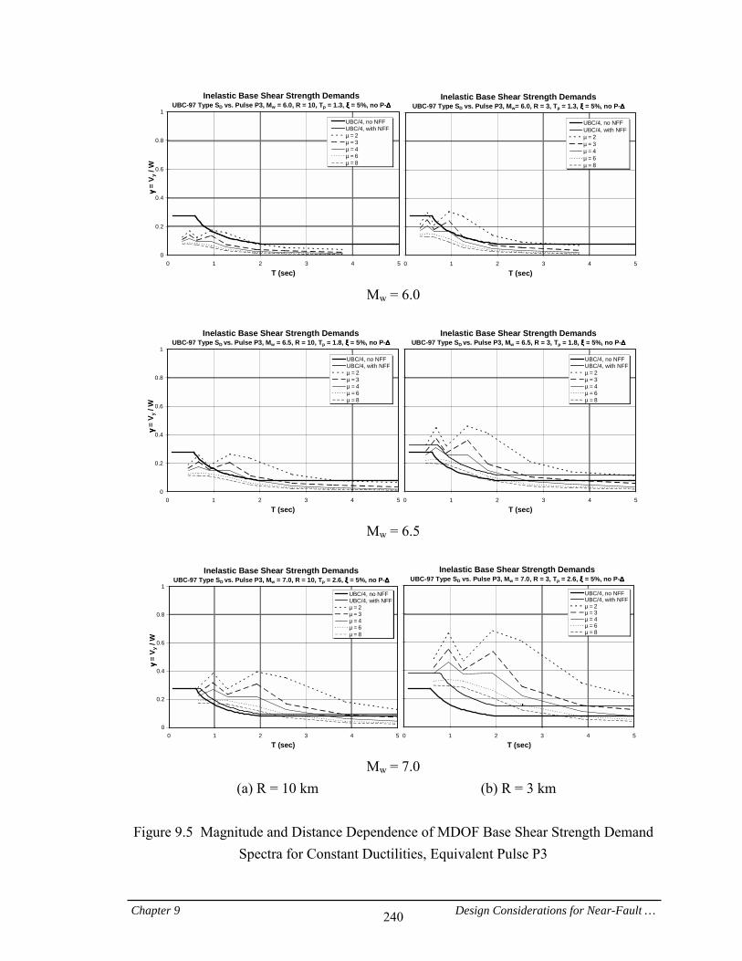
Chapter 9 Design Considerations for Near-Fault … 240
Inelastic Base Shear Strength DemandsUBC-97 Type SD vs. Pulse P3, Mw = 6.0, R = 10, Tp = 1.3, ξξξξ = 5%, no P-∆∆∆∆
0
0.2
0.4
0.6
0.8
1
0 1 2 3 4 5
T (sec)
γγ γγ =
V y /
W
UBC/4, no NFFUBC/4, with NFFµ===2µ===3µ===4µ===6µ===8
Inelastic Base Shear Strength DemandsUBC-97 Type SD vs. Pulse P3, Mw= 6.0, R = 3, Tp = 1.3, ξξξξ = 5%, no P-∆∆∆∆
0 1 2 3 4 5
T (sec)
UBC/4, no NFFUBC/4, with NFFµ===2µ===3µ===4µ===6µ===8
Mw = 6.0
Inelastic Base Shear Strength Demands
UBC-97 Type SD vs. Pulse P3, Mw = 6.5, R = 10, Tp = 1.8, ξξξξ = 5%, no P-∆∆∆∆
0
0.2
0.4
0.6
0.8
1
0 1 2 3 4 5
T (sec)
γγ γγ =
V y /
W
UBC/4, no NFFUBC/4, with NFFµ===2µ===3µ===4µ===6µ===8
Inelastic Base Shear Strength DemandsUBC-97 Type SD vs. Pulse P3, Mw = 6.5, R = 3, Tp = 1.8, ξξξξ = 5%, no P-∆∆∆∆
0 1 2 3 4 5
T (sec)
UBC/4, no NFFUBC/4, with NFFµ===2µ===3µ===4µ===6µ===8
Mw = 6.5
Inelastic Base Shear Strength Demands
UBC-97 Type SD vs. Pulse P3, Mw = 7.0, R = 10, Tp = 2.6, ξξξξ = 5%, no P-∆∆∆∆
0
0.2
0.4
0.6
0.8
1
0 1 2 3 4 5
T (sec)
γγ γγ =
V y /
W
UBC/4, no NFFUBC/4, with NFFµ===2µ===3µ===4µ===6µ===8
Inelastic Base Shear Strength DemandsUBC-97 Type SD vs. Pulse P3, Mw = 7.0, R = 3, Tp = 2.6, ξξξξ = 5%, no P-∆∆∆∆
0 1 2 3 4 5
T (sec)
UBC/4, no NFFUBC/4, with NFFµ===2µ===3µ===4µ===6µ===8
Mw = 7.0
(a) R = 10 km (b) R = 3 km
Figure 9.5 Magnitude and Distance Dependence of MDOF Base Shear Strength Demand Spectra for Constant Ductilities, Equivalent Pulse P3
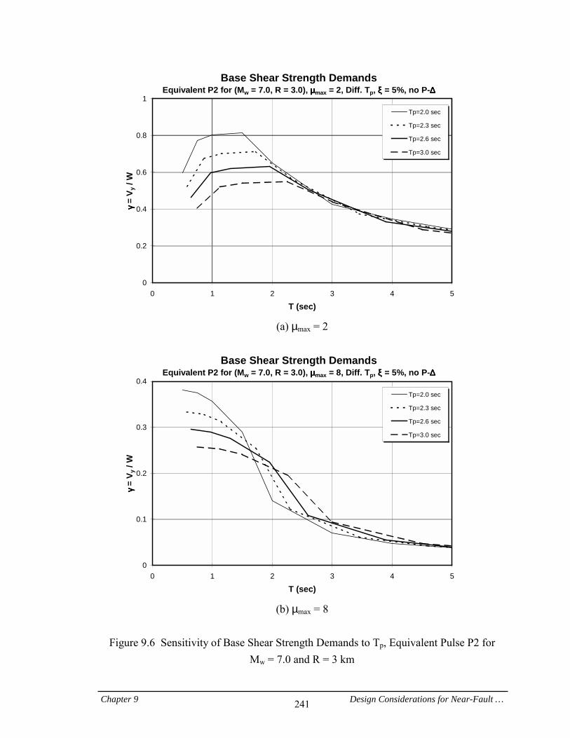
Chapter 9 Design Considerations for Near-Fault … 241
Base Shear Strength DemandsEquivalent P2 for (Mw = 7.0, R = 3.0), µµµµmax = 2, Diff. Tp, ξξξξ = 5%, no P-∆∆∆∆
0
0.2
0.4
0.6
0.8
1
0 1 2 3 4 5
T (sec)
γγ γγ =
V y /
W
Tp=2.0 sec
Tp=2.3 sec
Tp=2.6 sec
Tp=3.0 sec
(a) µmax = 2
Base Shear Strength Demands
Equivalent P2 for (Mw = 7.0, R = 3.0), µµµµmax = 8, Diff. Tp, ξξξξ = 5%, no P-∆∆∆∆
0
0.1
0.2
0.3
0.4
0 1 2 3 4 5
T (sec)
γγ γγ =
V y /
W
Tp=2.0 sec
Tp=2.3 sec
Tp=2.6 sec
Tp=3.0 sec
(b) µmax = 8
Figure 9.6 Sensitivity of Base Shear Strength Demands to Tp, Equivalent Pulse P2 for
Mw = 7.0 and R = 3 km
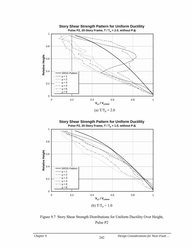
Chapter 9 Design Considerations for Near-Fault … 242
Story Shear Strength Pattern for Uniform DuctilityPulse P2, 20-Story Frame, T / Tp = 2.0, without P-∆∆∆∆
0
0.2
0.4
0.6
0.8
1
0 0.2 0.4 0.6 0.8 1Vy,i / Vy,base
Rel
ativ
e H
eigh
t
SRSS Patternµ===1µ===2µ===3µ===4µ===6µ===8
(a) T/Tp = 2.0
Story Shear Strength Pattern for Uniform Ductility
Pulse P2, 20-Story Frame, T / Tp = 1.0, without P-∆∆∆∆
0
0.2
0.4
0.6
0.8
1
0 0.2 0.4 0.6 0.8 1Vy,i / Vy,base
Rel
ativ
e H
eigh
t
SRSS Patternµ===1=µ===2µ===3µ===4=µ===6µ===8
(b) T/Tp = 1.0
Figure 9.7 Story Shear Strength Distributions for Uniform Ductility Over Height,
Pulse P2
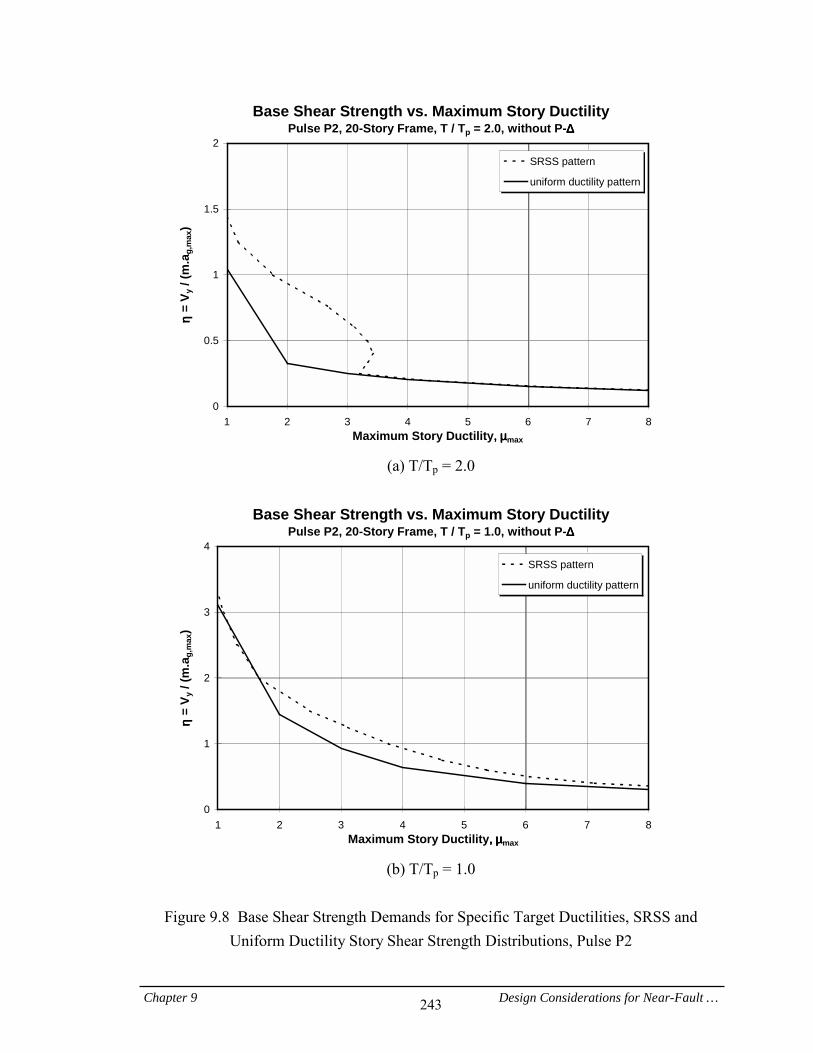
Chapter 9 Design Considerations for Near-Fault … 243
Base Shear Strength vs. Maximum Story DuctilityPulse P2, 20-Story Frame, T / Tp = 2.0, without P-∆∆∆∆
0
0.5
1
1.5
2
1 2 3 4 5 6 7 8Maximum Story Ductility,,,,====µµµµmax
ηη ηη =
V y /
(m.a
g,m
ax)
SRSS pattern
uniform ductility pattern
(a) T/Tp = 2.0
Base Shear Strength vs. Maximum Story Ductility
Pulse P2, 20-Story Frame, T / Tp = 1.0, without P-∆∆∆∆
0
1
2
3
4
1 2 3 4 5 6 7 8Maximum Story Ductility,,,,====µµµµmax
ηη ηη =
V y /
(m.a
g,m
ax)
SRSS pattern
uniform ductility pattern
(b) T/Tp = 1.0
Figure 9.8 Base Shear Strength Demands for Specific Target Ductilities, SRSS and
Uniform Ductility Story Shear Strength Distributions, Pulse P2
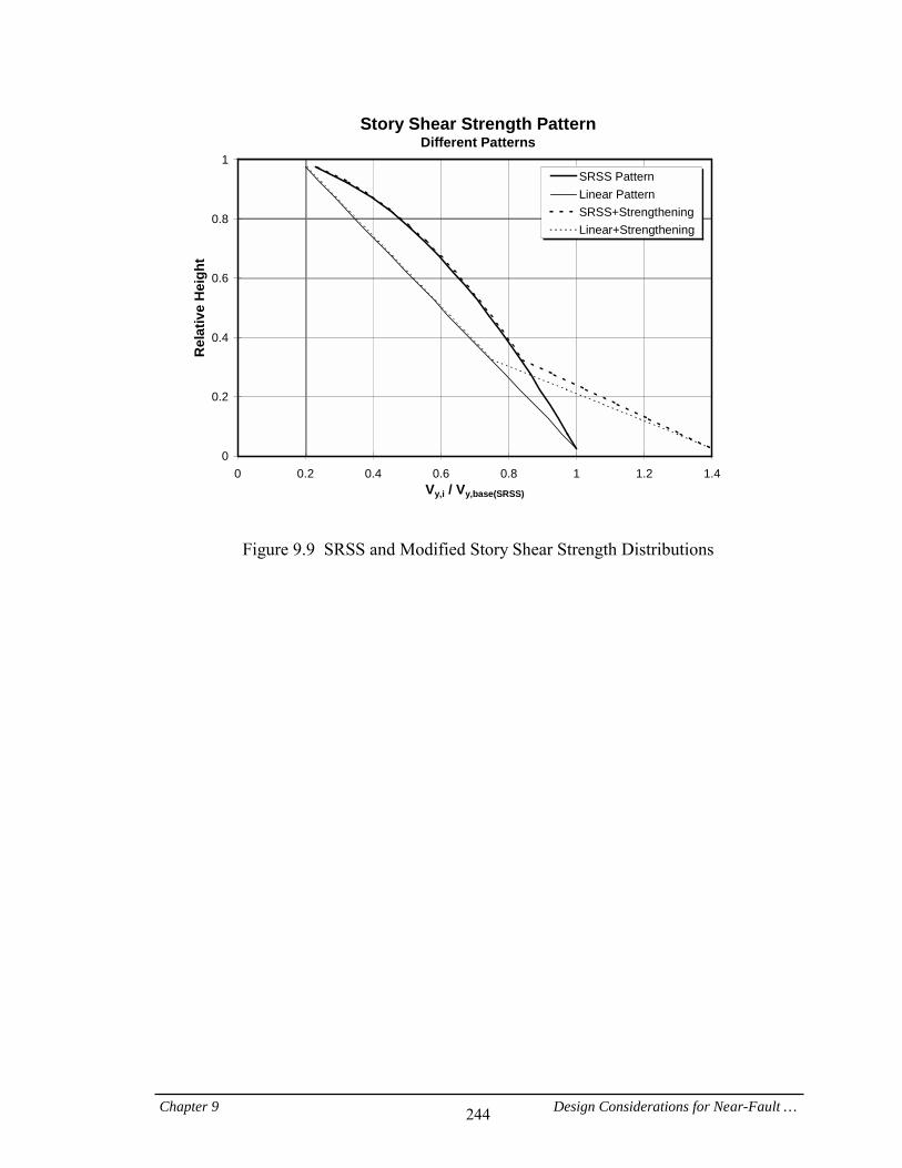
Chapter 9 Design Considerations for Near-Fault … 244
Story Shear Strength PatternDifferent Patterns
0
0.2
0.4
0.6
0.8
1
0 0.2 0.4 0.6 0.8 1 1.2 1.4Vy,i / Vy,base(SRSS)
Rel
ativ
e H
eigh
tSRSS PatternLinear PatternSRSS+StrengtheningLinear+Strengthening
Figure 9.9 SRSS and Modified Story Shear Strength Distributions
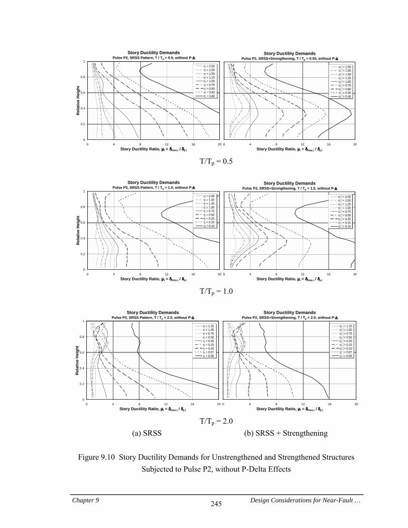
Chapter 9 Design Considerations for Near-Fault … 245
Story Ductility DemandsPulse P2, SRSS Pattern, T / Tp = 0.5, without P-∆∆∆∆
0
0.2
0.4
0.6
0.8
1
0 4 8 12 16 20Story Ductility Ratio, µµµµi = δδδδmax,i / δδδδy,i
Rel
ativ
e H
eigh
t
η===2.50η===2.00η===1.50η===1.25η===1.00η===0.75η===0.60η===0.50η===0.40
Story Ductility DemandsPulse P2, SRSS+Strengthening, T / Tp = 0.50, without P-∆∆∆∆
0 4 8 12 16 20Story Ductility Ratio, µµµµi = δδδδmax,i / δδδδy,i
η∗ ===2.50η∗ ===2.00η∗ ===1.50η∗ ===1.25η∗ ===1.00η∗ ===0.75η∗ ===0.60η∗ ===0.50η∗ ===0.40
T/Tp = 0.5
Story Ductility Demands
Pulse P2, SRSS Pattern, T / Tp = 1.0, without P-∆∆∆∆
0
0.2
0.4
0.6
0.8
1
0 4 8 12 16 20Story Ductility Ratio, µµµµi = δδδδmax,i / δδδδy,i
Rel
ativ
e H
eigh
t
η===2.00η===1.50η===1.25η===1.00η===0.75η===0.50η===0.25η===0.15η===0.10
Story Ductility DemandsPulse P2, SRSS+Strengthening, T / Tp = 1.0, without P-∆∆∆∆
0 4 8 12 16 20Story Ductility Ratio, µµµµi = δδδδmax,i / δδδδy,i
η∗ ===2.00η∗ ===1.50η∗ ===1.25η∗ ===1.00η∗ ===0.75η∗ ===0.50η∗ ===0.25η∗ ===0.15η∗ ===0.10
T/Tp = 1.0
Story Ductility Demands
Pulse P2, SRSS Pattern, T / Tp = 2.0, without P-∆∆∆∆
0
0.2
0.4
0.6
0.8
1
0 4 8 12 16 20Story Ductility Ratio, µµµµi = δδδδmax,i / δδδδy,i
Rel
ativ
e H
eigh
t
η===1.25η===1.00η===0.75η===0.50η===0.25η===0.15η===0.10η===0.07η===0.05
Story Ductility DemandsPulse P2, SRSS+Strengthening, T / Tp = 2.0, without P-∆∆∆∆
0 4 8 12 16 20Story Ductility Ratio, µµµµi = δδδδmax,i / δδδδy,i
η∗ ===1.25η∗ ===1.00η∗ ===0.75η∗ ===0.50η∗ ===0.25η∗ ===0.15η∗ ===0.10η∗ ===0.07η∗ ===0.05
T/Tp = 2.0
(a) SRSS (b) SRSS + Strengthening
Figure 9.10 Story Ductility Demands for Unstrengthened and Strengthened Structures Subjected to Pulse P2, without P-Delta Effects
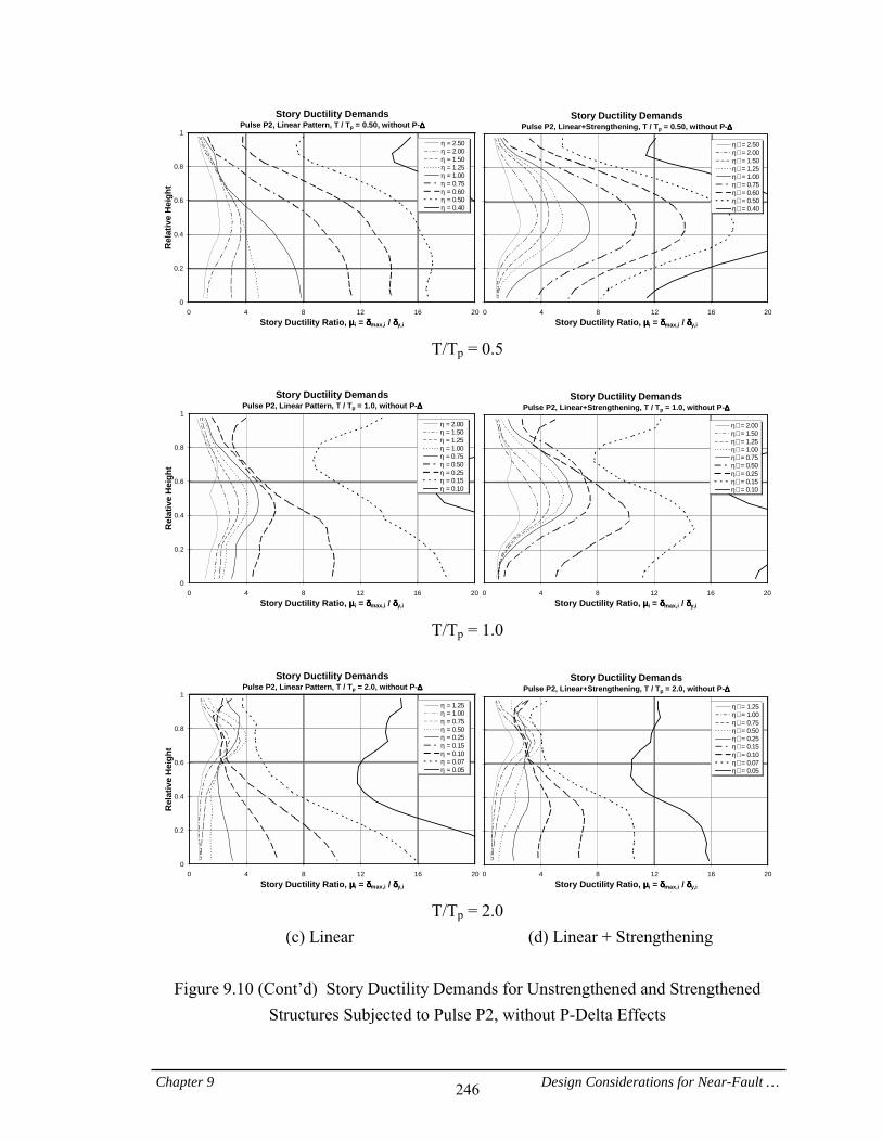
Chapter 9 Design Considerations for Near-Fault … 246
Story Ductility DemandsPulse P2, Linear Pattern, T / Tp = 0.50, without P-∆∆∆∆
0
0.2
0.4
0.6
0.8
1
0 4 8 12 16 20Story Ductility Ratio, µµµµi = δδδδmax,i / δδδδy,i
Rel
ativ
e H
eigh
t
η===2.50η===2.00η===1.50η===1.25η===1.00η===0.75η===0.60η===0.50η===0.40
Story Ductility DemandsPulse P2, Linear+Strengthening, T / Tp = 0.50, without P-∆∆∆∆
0 4 8 12 16 20Story Ductility Ratio, µµµµi = δδδδmax,i / δδδδy,i
η∗ ===2.50η∗ ===2.00η∗ ===1.50η∗ ===1.25η∗ ===1.00η∗ ===0.75η∗ ===0.60η∗ ===0.50η∗ ===0.40
T/Tp = 0.5
Story Ductility Demands
Pulse P2, Linear Pattern, T / Tp = 1.0, without P-∆∆∆∆
0
0.2
0.4
0.6
0.8
1
0 4 8 12 16 20Story Ductility Ratio, µµµµi = δδδδmax,i / δδδδy,i
Rel
ativ
e H
eigh
t
η===2.00η===1.50η===1.25η===1.00η===0.75η===0.50η===0.25η===0.15η===0.10
Story Ductility DemandsPulse P2, Linear+Strengthening, T / Tp = 1.0, without P-∆∆∆∆
0 4 8 12 16 20Story Ductility Ratio, µµµµi = δδδδmax,i / δδδδy,i
η∗ ===2.00η∗ ===1.50η∗ ===1.25η∗ ===1.00η∗ ===0.75η∗ ===0.50η∗ ===0.25η∗ ===0.15η∗ ===0.10
T/Tp = 1.0
Story Ductility Demands
Pulse P2, Linear Pattern, T / Tp = 2.0, without P-∆∆∆∆
0
0.2
0.4
0.6
0.8
1
0 4 8 12 16 20Story Ductility Ratio, µµµµi = δδδδmax,i / δδδδy,i
Rel
ativ
e H
eigh
t
η===1.25η===1.00η===0.75η===0.50η===0.25η===0.15η===0.10η===0.07η===0.05
Story Ductility DemandsPulse P2, Linear+Strengthening, T / Tp = 2.0, without P-∆∆∆∆
0 4 8 12 16 20Story Ductility Ratio, µµµµi = δδδδmax,i / δδδδy,i
η∗ ===1.25η∗ ===1.00η∗ ===0.75η∗ ===0.50η∗ ===0.25η∗ ===0.15η∗ ===0.10η∗ ===0.07η∗ ===0.05
T/Tp = 2.0
(c) Linear (d) Linear + Strengthening
Figure 9.10 (Cont’d) Story Ductility Demands for Unstrengthened and Strengthened Structures Subjected to Pulse P2, without P-Delta Effects
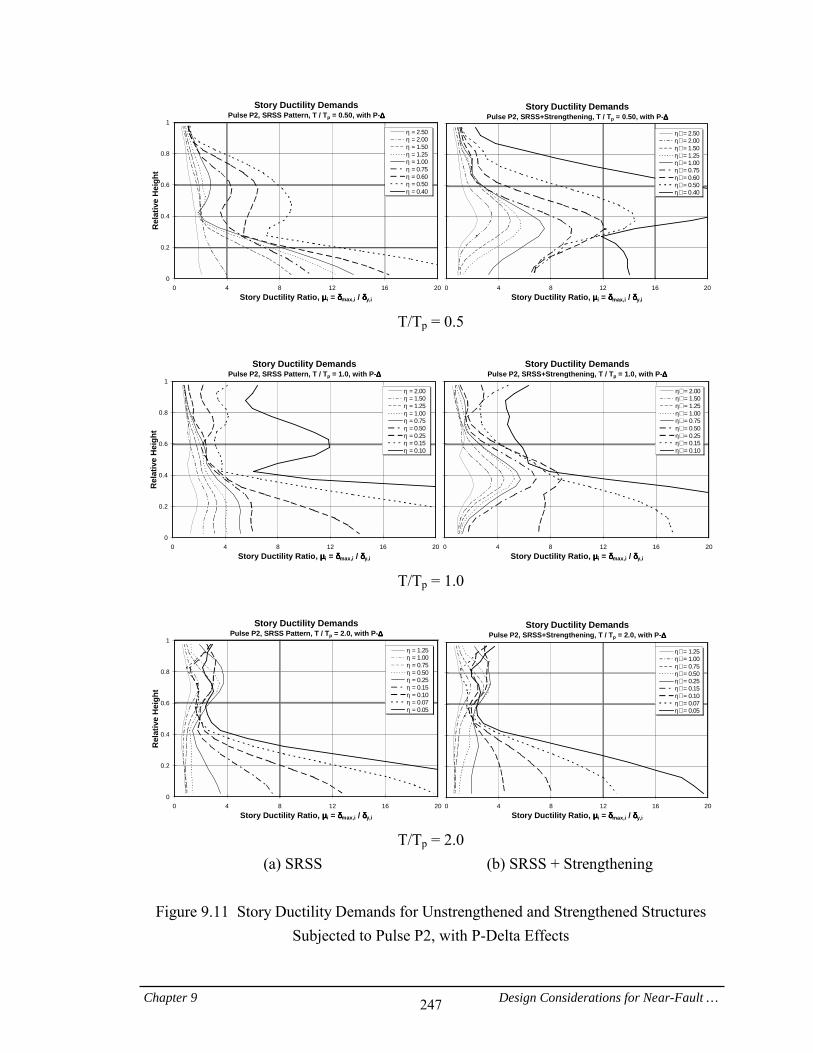
Chapter 9 Design Considerations for Near-Fault … 247
Story Ductility DemandsPulse P2, SRSS Pattern, T / Tp = 0.50, with P-∆∆∆∆
0
0.2
0.4
0.6
0.8
1
0 4 8 12 16 20Story Ductility Ratio, µµµµi = δδδδmax,i / δδδδy,i
Rel
ativ
e H
eigh
t
η===2.50η===2.00η===1.50η===1.25η===1.00η===0.75η===0.60η===0.50η===0.40
Story Ductility DemandsPulse P2, SRSS+Strengthening, T / Tp = 0.50, with P-∆∆∆∆
0 4 8 12 16 20Story Ductility Ratio, µµµµi = δδδδmax,i / δδδδy,i
η∗ ===2.50η∗ ===2.00η∗ ===1.50η∗ ===1.25η∗ ===1.00η∗ ===0.75η∗ ===0.60η∗ ===0.50η∗ ===0.40
T/Tp = 0.5
Story Ductility Demands
Pulse P2, SRSS Pattern, T / Tp = 1.0, with P-∆∆∆∆
0
0.2
0.4
0.6
0.8
1
0 4 8 12 16 20Story Ductility Ratio, µµµµi = δδδδmax,i / δδδδy,i
Rel
ativ
e H
eigh
t
η===2.00η===1.50η===1.25η===1.00η===0.75η===0.50η===0.25η===0.15η===0.10
Story Ductility DemandsPulse P2, SRSS+Strengthening, T / Tp = 1.0, with P-∆∆∆∆
0 4 8 12 16 20Story Ductility Ratio, µµµµi = δδδδmax,i / δδδδy,i
η∗ ===2.00η∗ ===1.50η∗ ===1.25η∗ ===1.00η∗ ===0.75η∗ ===0.50η∗ ===0.25η∗ ===0.15η∗ ===0.10
T/Tp = 1.0
Story Ductility Demands
Pulse P2, SRSS Pattern, T / Tp = 2.0, with P-∆∆∆∆
0
0.2
0.4
0.6
0.8
1
0 4 8 12 16 20Story Ductility Ratio, µµµµi = δδδδmax,i / δδδδy,i
Rel
ativ
e H
eigh
t
η===1.25η===1.00η===0.75η===0.50η===0.25η===0.15η===0.10η===0.07η===0.05
Story Ductility DemandsPulse P2, SRSS+Strengthening, T / Tp = 2.0, with P-∆∆∆∆
0 4 8 12 16 20Story Ductility Ratio, µµµµi = δδδδmax,i / δδδδy,i
η∗ ===1.25η∗ ===1.00η∗ ===0.75η∗ ===0.50η∗ ===0.25η∗ ===0.15η∗ ===0.10η∗ ===0.07η∗ ===0.05
T/Tp = 2.0
(a) SRSS (b) SRSS + Strengthening
Figure 9.11 Story Ductility Demands for Unstrengthened and Strengthened Structures Subjected to Pulse P2, with P-Delta Effects
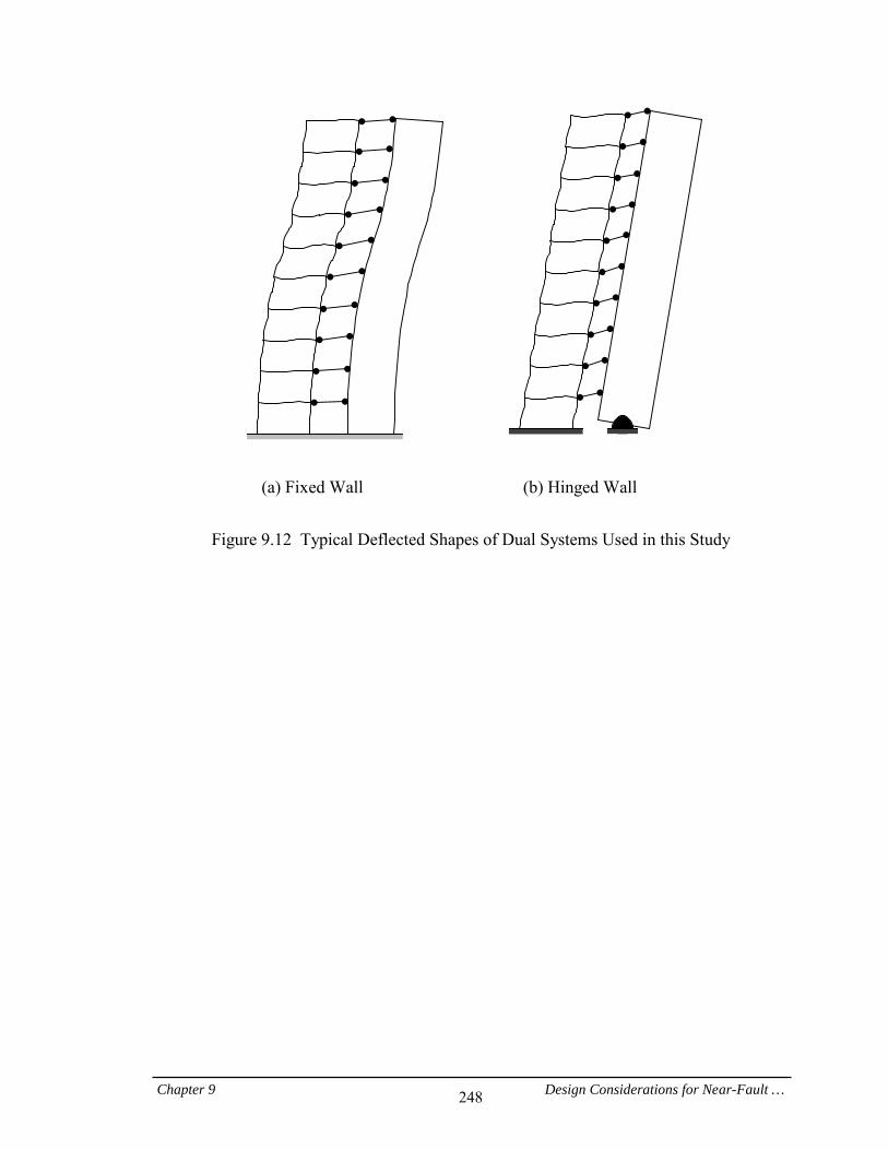
Chapter 9 Design Considerations for Near-Fault … 248
(a) Fixed Wall (b) Hinged Wall
Figure 9.12 Typical Deflected Shapes of Dual Systems Used in this Study
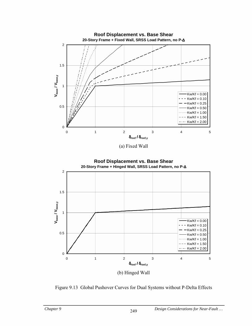
Chapter 9 Design Considerations for Near-Fault … 249
Roof Displacement vs. Base Shear20-Story Frame + Fixed Wall, SRSS Load Pattern, no P-∆∆∆∆====
0
0.5
1
1.5
2
0 1 2 3 4 5δδδδroof====////====δδδδroof,y
V bas
e / V
base
,y
Kw/Kf = 0.00Kw/Kf = 0.10Kw/Kf = 0.25Kw/Kf = 0.50Kw/Kf = 1.00Kw/Kf = 1.50Kw/Kf = 2.00
(a) Fixed Wall
Roof Displacement vs. Base Shear
20-Story Frame + Hinged Wall, SRSS Load Pattern, no P-∆∆∆∆====
0
0.5
1
1.5
2
0 1 2 3 4 5δδδδroof====////====δδδδroof,y
V bas
e / V
base
,y
Kw/Kf = 0.00Kw/Kf = 0.10Kw/Kf = 0.25Kw/Kf = 0.50Kw/Kf = 1.00Kw/Kf = 1.50Kw/Kf = 2.00
(b) Hinged Wall
Figure 9.13 Global Pushover Curves for Dual Systems without P-Delta Effects
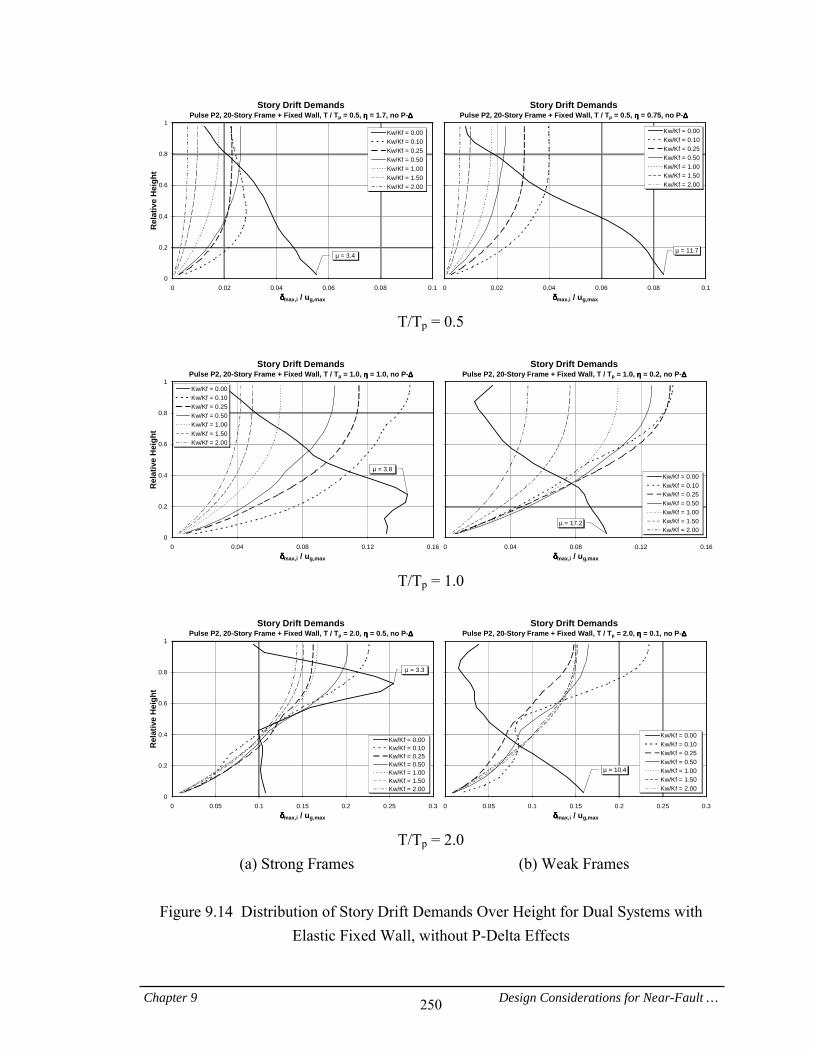
Chapter 9 Design Considerations for Near-Fault … 250
Story Drift DemandsPulse P2, 20-Story Frame + Fixed Wall, T / Tp = 0.5, ηηηη = 1.7, no P-∆∆∆∆
0
0.2
0.4
0.6
0.8
1
0 0.02 0.04 0.06 0.08 0.1δδδδmax,i / ug,max
Rel
ativ
e H
eigh
t
Kw/Kf = 0.00Kw/Kf = 0.10Kw/Kf = 0.25Kw/Kf = 0.50Kw/Kf = 1.00Kw/Kf = 1.50Kw/Kf = 2.00
µ = 3.4
Story Drift DemandsPulse P2, 20-Story Frame + Fixed Wall, T / Tp = 0.5, ηηηη = 0.75, no P-∆∆∆∆
0 0.02 0.04 0.06 0.08 0.1δδδδmax,i / ug,max
Kw/Kf = 0.00Kw/Kf = 0.10Kw/Kf = 0.25Kw/Kf = 0.50Kw/Kf = 1.00Kw/Kf = 1.50Kw/Kf = 2.00
µ = 11.7
T/Tp = 0.5
Story Drift Demands
Pulse P2, 20-Story Frame + Fixed Wall, T / Tp = 1.0, ηηηη = 1.0, no P-∆∆∆∆
0
0.2
0.4
0.6
0.8
1
0 0.04 0.08 0.12 0.16δδδδmax,i / ug,max
Rel
ativ
e H
eigh
t
Kw/Kf = 0.00Kw/Kf = 0.10Kw/Kf = 0.25Kw/Kf = 0.50Kw/Kf = 1.00Kw/Kf = 1.50Kw/Kf = 2.00
µ = 3.8
Story Drift DemandsPulse P2, 20-Story Frame + Fixed Wall, T / Tp = 1.0, ηηηη = 0.2, no P-∆∆∆∆
0 0.04 0.08 0.12 0.16δδδδmax,i / ug,max
Kw/Kf = 0.00Kw/Kf = 0.10Kw/Kf = 0.25Kw/Kf = 0.50Kw/Kf = 1.00Kw/Kf = 1.50Kw/Kf = 2.00
µ = 17.2
T/Tp = 1.0
Story Drift Demands
Pulse P2, 20-Story Frame + Fixed Wall, T / Tp = 2.0, ηηηη = 0.5, no P-∆∆∆∆
0
0.2
0.4
0.6
0.8
1
0 0.05 0.1 0.15 0.2 0.25 0.3δδδδmax,i / ug,max
Rel
ativ
e H
eigh
t
Kw/Kf = 0.00Kw/Kf = 0.10Kw/Kf = 0.25Kw/Kf = 0.50Kw/Kf = 1.00Kw/Kf = 1.50Kw/Kf = 2.00
µ = 3.3
Story Drift DemandsPulse P2, 20-Story Frame + Fixed Wall, T / Tp = 2.0, ηηηη = 0.1, no P-∆∆∆∆
0 0.05 0.1 0.15 0.2 0.25 0.3δδδδmax,i / ug,max
Kw/Kf = 0.00Kw/Kf = 0.10Kw/Kf = 0.25Kw/Kf = 0.50Kw/Kf = 1.00Kw/Kf = 1.50Kw/Kf = 2.00
µ = 10.4
T/Tp = 2.0
(a) Strong Frames (b) Weak Frames
Figure 9.14 Distribution of Story Drift Demands Over Height for Dual Systems with Elastic Fixed Wall, without P-Delta Effects

Chapter 9 Design Considerations for Near-Fault … 251
Story Drift DemandsPulse P2, 20-Story Frame + Hinged Wall, T / Tp = 0.5, ηηηη = 1.7, no P-∆∆∆∆
0
0.2
0.4
0.6
0.8
1
0 0.02 0.04 0.06 0.08 0.1δδδδmax,i / ug,max
Rel
ativ
e H
eigh
t
Kw/Kf = 0.00Kw/Kf = 0.10Kw/Kf = 0.25Kw/Kf = 0.50Kw/Kf = 1.00Kw/Kf = 1.50Kw/Kf = 2.00
µ = 3.4
Story Drift DemandsPulse P2, 20-Story Frame + Hinged Wall, T / Tp = 0.5, ηηηη = 0.75, no P-∆∆∆∆
0 0.02 0.04 0.06 0.08 0.1δδδδmax,i / ug,max
Kw/Kf = 0.00Kw/Kf = 0.10Kw/Kf = 0.25Kw/Kf = 0.50Kw/Kf = 1.00Kw/Kf = 1.50Kw/Kf = 2.00
µ = 11.7
T/Tp = 0.5
Story Drift Demands
Pulse P2, 20-Story Frame + Hinged Wall, T / Tp = 1.0, ηηηη = 1.0, no P-∆∆∆∆
0
0.2
0.4
0.6
0.8
1
0 0.04 0.08 0.12 0.16δδδδmax,i / ug,max
Rel
ativ
e H
eigh
t
Kw/Kf = 0.00Kw/Kf = 0.10Kw/Kf = 0.25Kw/Kf = 0.50Kw/Kf = 1.00Kw/Kf = 1.50Kw/Kf = 2.00
µ = 3.8
Story Drift DemandsPulse P2, 20-Story Frame + Hinged Wall, T / Tp = 1.0, ηηηη = 0.2, no P-∆∆∆∆
0 0.04 0.08 0.12 0.16δδδδmax,i / ug,max
Kw/Kf = 0.00Kw/Kf = 0.10Kw/Kf = 0.25Kw/Kf = 0.50Kw/Kf = 1.00Kw/Kf = 1.50Kw/Kf = 2.00
µ = 17.2
T/Tp = 1.0
Story Drift Demands
Pulse P2, 20-Story Frame + Hinged Wall, T / Tp = 2.0, ηηηη = 0.5, no P-∆∆∆∆
0
0.2
0.4
0.6
0.8
1
0 0.05 0.1 0.15 0.2 0.25 0.3δδδδmax,i / ug,max
Rel
ativ
e H
eigh
t
Kw/Kf = 0.00Kw/Kf = 0.10Kw/Kf = 0.25Kw/Kf = 0.50Kw/Kf = 1.00Kw/Kf = 1.50Kw/Kf = 2.00
µ = 3.3
Story Drift DemandsPulse P2, 20-Story Frame + Hinged Wall, T / Tp = 2.0, ηηηη = 0.1, no P-∆∆∆∆
0 0.05 0.1 0.15 0.2 0.25 0.3δδδδmax,i / ug,max
Kw/Kf = 0.00Kw/Kf = 0.10Kw/Kf = 0.25Kw/Kf = 0.50Kw/Kf = 1.00Kw/Kf = 1.50Kw/Kf = 2.00
µ = 10.4
T/Tp = 2.0
(a) Strong Frames (b) Weak Frames
Figure 9.15 Distribution of Story Drift Demands Over Height for Dual Systems with Elastic Hinged Wall, without P-Delta Effects
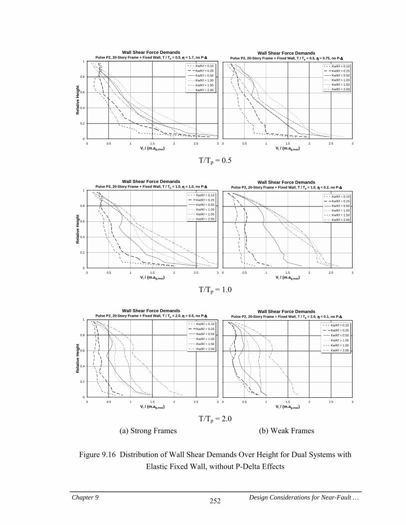
Chapter 9 Design Considerations for Near-Fault … 252
Wall Shear Force DemandsPulse P2, 20-Story Frame + Fixed Wall, T / Tp = 0.5, ηηηη = 1.7, no P-∆∆∆∆
0
0.2
0.4
0.6
0.8
1
0 0.5 1 1.5 2 2.5 3Vi / (m.ag,max)
Rel
ativ
e H
eigh
t
Kw/Kf = 0.10Kw/Kf = 0.25Kw/Kf = 0.50Kw/Kf = 1.00Kw/Kf = 1.50Kw/Kf = 2.00
Wall Shear Force DemandsPulse P2, 20-Story Frame + Fixed Wall, T / Tp = 0.5, ηηηη = 0.75, no P-∆∆∆∆
0 0.5 1 1.5 2 2.5 3Vi / (m.ag,max)
Kw/Kf = 0.10Kw/Kf = 0.25Kw/Kf = 0.50Kw/Kf = 1.00Kw/Kf = 1.50Kw/Kf = 2.00
T/Tp = 0.5
Wall Shear Force Demands
Pulse P2, 20-Story Frame + Fixed Wall, T / Tp = 1.0, ηηηη = 1.0, no P-∆∆∆∆
0
0.2
0.4
0.6
0.8
1
0 0.5 1 1.5 2 2.5 3Vi / (m.ag,max)
Rel
ativ
e H
eigh
t
Kw/Kf = 0.10Kw/Kf = 0.25Kw/Kf = 0.50Kw/Kf = 1.00Kw/Kf = 1.50Kw/Kf = 2.00
Wall Shear Force DemandsPulse P2, 20-Story Frame + Fixed Wall, T / Tp = 1.0, ηηηη = 0.2, no P-∆∆∆∆
0 0.5 1 1.5 2 2.5 3Vi / (m.ag,max)
Kw/Kf = 0.10Kw/Kf = 0.25Kw/Kf = 0.50Kw/Kf = 1.00Kw/Kf = 1.50Kw/Kf = 2.00
T/Tp = 1.0
Wall Shear Force Demands
Pulse P2, 20-Story Frame + Fixed Wall, T / Tp = 2.0, ηηηη = 0.5, no P-∆∆∆∆
0
0.2
0.4
0.6
0.8
1
0 0.5 1 1.5 2 2.5 3Vi / (m.ag,max)
Rel
ativ
e H
eigh
t
Kw/Kf = 0.10Kw/Kf = 0.25Kw/Kf = 0.50Kw/Kf = 1.00Kw/Kf = 1.50Kw/Kf = 2.00
Wall Shear Force DemandsPulse P2, 20-Story Frame + Fixed Wall, T / Tp = 2.0, ηηηη = 0.1, no P-∆∆∆∆
0 0.5 1 1.5 2 2.5 3Vi / (m.ag,max)
Kw/Kf = 0.10Kw/Kf = 0.25Kw/Kf = 0.50Kw/Kf = 1.00Kw/Kf = 1.50Kw/Kf = 2.00
T/Tp = 2.0
(a) Strong Frames (b) Weak Frames
Figure 9.16 Distribution of Wall Shear Demands Over Height for Dual Systems with Elastic Fixed Wall, without P-Delta Effects
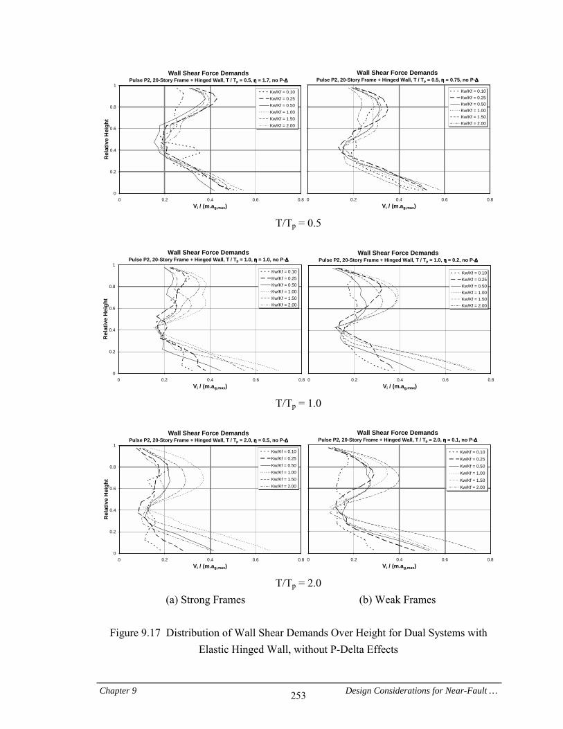
Chapter 9 Design Considerations for Near-Fault … 253
Wall Shear Force DemandsPulse P2, 20-Story Frame + Hinged Wall, T / Tp = 0.5, ηηηη = 1.7, no P-∆∆∆∆
0
0.2
0.4
0.6
0.8
1
0 0.2 0.4 0.6 0.8Vi / (m.ag,max)
Rel
ativ
e H
eigh
t
Kw/Kf = 0.10Kw/Kf = 0.25Kw/Kf = 0.50Kw/Kf = 1.00Kw/Kf = 1.50Kw/Kf = 2.00
Wall Shear Force DemandsPulse P2, 20-Story Frame + Hinged Wall, T / Tp = 0.5, ηηηη = 0.75, no P-∆∆∆∆
0 0.2 0.4 0.6 0.8Vi / (m.ag,max)
Kw/Kf = 0.10Kw/Kf = 0.25Kw/Kf = 0.50Kw/Kf = 1.00Kw/Kf = 1.50Kw/Kf = 2.00
T/Tp = 0.5
Wall Shear Force Demands
Pulse P2, 20-Story Frame + Hinged Wall, T / Tp = 1.0, ηηηη = 1.0, no P-∆∆∆∆
0
0.2
0.4
0.6
0.8
1
0 0.2 0.4 0.6 0.8Vi / (m.ag,max)
Rel
ativ
e H
eigh
t
Kw/Kf = 0.10Kw/Kf = 0.25Kw/Kf = 0.50Kw/Kf = 1.00Kw/Kf = 1.50Kw/Kf = 2.00
Wall Shear Force DemandsPulse P2, 20-Story Frame + Hinged Wall, T / Tp = 1.0, ηηηη = 0.2, no P-∆∆∆∆
0 0.2 0.4 0.6 0.8Vi / (m.ag,max)
Kw/Kf = 0.10Kw/Kf = 0.25Kw/Kf = 0.50Kw/Kf = 1.00Kw/Kf = 1.50Kw/Kf = 2.00
T/Tp = 1.0
Wall Shear Force Demands
Pulse P2, 20-Story Frame + Hinged Wall, T / Tp = 2.0, ηηηη = 0.5, no P-∆∆∆∆
0
0.2
0.4
0.6
0.8
1
0 0.2 0.4 0.6 0.8Vi / (m.ag,max)
Rel
ativ
e H
eigh
t
Kw/Kf = 0.10Kw/Kf = 0.25Kw/Kf = 0.50Kw/Kf = 1.00Kw/Kf = 1.50Kw/Kf = 2.00
Wall Shear Force DemandsPulse P2, 20-Story Frame + Hinged Wall, T / Tp = 2.0, ηηηη = 0.1, no P-∆∆∆∆
0 0.2 0.4 0.6 0.8Vi / (m.ag,max)
Kw/Kf = 0.10Kw/Kf = 0.25Kw/Kf = 0.50Kw/Kf = 1.00Kw/Kf = 1.50Kw/Kf = 2.00
T/Tp = 2.0
(a) Strong Frames (b) Weak Frames
Figure 9.17 Distribution of Wall Shear Demands Over Height for Dual Systems with Elastic Hinged Wall, without P-Delta Effects
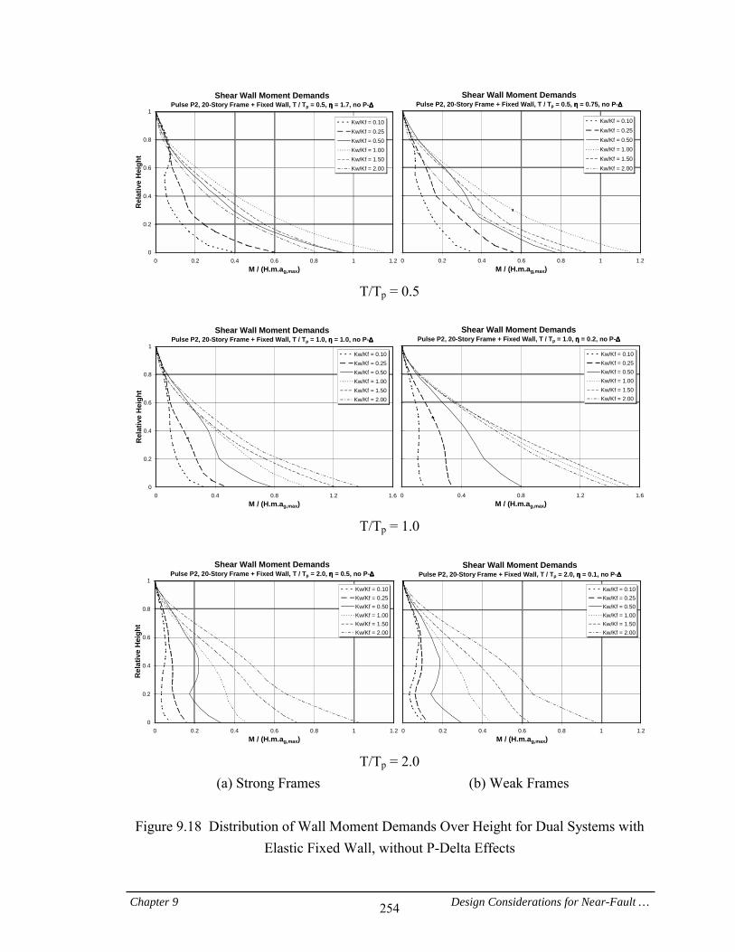
Chapter 9 Design Considerations for Near-Fault … 254
Shear Wall Moment DemandsPulse P2, 20-Story Frame + Fixed Wall, T / Tp = 0.5, ηηηη = 1.7, no P-∆∆∆∆
0
0.2
0.4
0.6
0.8
1
0 0.2 0.4 0.6 0.8 1 1.2M / (H.m.ag,max)
Rel
ativ
e H
eigh
t
Kw/Kf = 0.10Kw/Kf = 0.25Kw/Kf = 0.50Kw/Kf = 1.00Kw/Kf = 1.50Kw/Kf = 2.00
Shear Wall Moment DemandsPulse P2, 20-Story Frame + Fixed Wall, T / Tp = 0.5, ηηηη = 0.75, no P-∆∆∆∆
0 0.2 0.4 0.6 0.8 1 1.2M / (H.m.ag,max)
Kw/Kf = 0.10Kw/Kf = 0.25Kw/Kf = 0.50Kw/Kf = 1.00Kw/Kf = 1.50Kw/Kf = 2.00
T/Tp = 0.5
Shear Wall Moment Demands
Pulse P2, 20-Story Frame + Fixed Wall, T / Tp = 1.0, ηηηη = 1.0, no P-∆∆∆∆
0
0.2
0.4
0.6
0.8
1
0 0.4 0.8 1.2 1.6M / (H.m.ag,max)
Rel
ativ
e H
eigh
t
Kw/Kf = 0.10Kw/Kf = 0.25Kw/Kf = 0.50Kw/Kf = 1.00Kw/Kf = 1.50Kw/Kf = 2.00
Shear Wall Moment DemandsPulse P2, 20-Story Frame + Fixed Wall, T / Tp = 1.0, ηηηη = 0.2, no P-∆∆∆∆
0 0.4 0.8 1.2 1.6M / (H.m.ag,max)
Kw/Kf = 0.10Kw/Kf = 0.25Kw/Kf = 0.50Kw/Kf = 1.00Kw/Kf = 1.50Kw/Kf = 2.00
T/Tp = 1.0
Shear Wall Moment Demands
Pulse P2, 20-Story Frame + Fixed Wall, T / Tp = 2.0, ηηηη = 0.5, no P-∆∆∆∆
0
0.2
0.4
0.6
0.8
1
0 0.2 0.4 0.6 0.8 1 1.2M / (H.m.ag,max)
Rel
ativ
e H
eigh
t
Kw/Kf = 0.10Kw/Kf = 0.25Kw/Kf = 0.50Kw/Kf = 1.00Kw/Kf = 1.50Kw/Kf = 2.00
Shear Wall Moment DemandsPulse P2, 20-Story Frame + Fixed Wall, T / Tp = 2.0, ηηηη = 0.1, no P-∆∆∆∆
0 0.2 0.4 0.6 0.8 1 1.2M / (H.m.ag,max)
Kw/Kf = 0.10Kw/Kf = 0.25Kw/Kf = 0.50Kw/Kf = 1.00Kw/Kf = 1.50Kw/Kf = 2.00
T/Tp = 2.0
(a) Strong Frames (b) Weak Frames
Figure 9.18 Distribution of Wall Moment Demands Over Height for Dual Systems with Elastic Fixed Wall, without P-Delta Effects
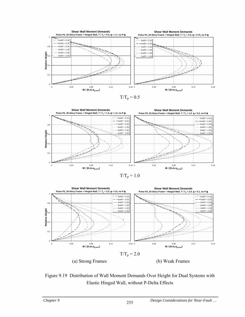
Chapter 9 Design Considerations for Near-Fault … 255
Shear Wall Moment DemandsPulse P2, 20-Story Frame + Hinged Wall, T / Tp = 0.5, ηηηη = 1.7, no P-∆∆∆∆
0
0.2
0.4
0.6
0.8
1
0 0.04 0.08 0.12 0.16M / (H.m.ag,max)
Rel
ativ
e H
eigh
t
Kw/Kf = 0.10Kw/Kf = 0.25Kw/Kf = 0.50Kw/Kf = 1.00Kw/Kf = 1.50Kw/Kf = 2.00
Shear Wall Moment DemandsPulse P2, 20-Story Frame + Hinged Wall, T / Tp = 0.5, ηηηη = 0.75, no P-∆∆∆∆
0 0.04 0.08 0.12 0.16M / (H.m.ag,max)
Kw/Kf = 0.10Kw/Kf = 0.25Kw/Kf = 0.50Kw/Kf = 1.00Kw/Kf = 1.50Kw/Kf = 2.00
T/Tp = 0.5
Shear Wall Moment Demands
Pulse P2, 20-Story Frame + Hinged Wall, T / Tp = 1.0, ηηηη = 1.0, no P-∆∆∆∆
0
0.2
0.4
0.6
0.8
1
0 0.04 0.08 0.12 0.16M / (H.m.ag,max)
Rel
ativ
e H
eigh
t
Kw/Kf = 0.10Kw/Kf = 0.25Kw/Kf = 0.50Kw/Kf = 1.00Kw/Kf = 1.50Kw/Kf = 2.00
Shear Wall Moment DemandsPulse P2, 20-Story Frame + Hinged Wall, T / Tp = 1.0, ηηηη = 0.2, no P-∆∆∆∆
0 0.04 0.08 0.12 0.16M / (H.m.ag,max)
Kw/Kf = 0.10Kw/Kf = 0.25Kw/Kf = 0.50Kw/Kf = 1.00Kw/Kf = 1.50Kw/Kf = 2.00
T/Tp = 1.0
Shear Wall Moment Demands
Pulse P2, 20-Story Frame + Hinged Wall, T / Tp = 2.0, ηηηη = 0.5, no P-∆∆∆∆
0
0.2
0.4
0.6
0.8
1
0 0.04 0.08 0.12 0.16M / (H.m.ag,max)
Rel
ativ
e H
eigh
t
Kw/Kf = 0.10Kw/Kf = 0.25Kw/Kf = 0.50Kw/Kf = 1.00Kw/Kf = 1.50Kw/Kf = 2.00
Shear Wall Moment DemandsPulse P2, 20-Story Frame + Hinged Wall, T / Tp = 2.0, ηηηη = 0.1, no P-∆∆∆∆
0 0.04 0.08 0.12 0.16M / (H.m.ag,max)
Kw/Kf = 0.10Kw/Kf = 0.25Kw/Kf = 0.50Kw/Kf = 1.00Kw/Kf = 1.50Kw/Kf = 2.00
T/Tp = 2.0
(a) Strong Frames (b) Weak Frames Figure 9.19 Distribution of Wall Moment Demands Over Height for Dual Systems with
Elastic Hinged Wall, without P-Delta Effects
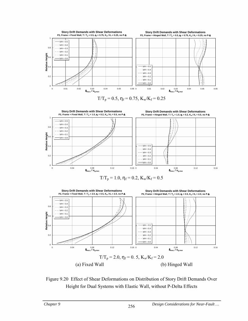
Chapter 9 Design Considerations for Near-Fault … 256
Story Drift Demands with Shear DeformationsP2, Frame + Fixed Wall, T / Tp = 0.5, ηηηηf = 0.75, Kw / Kf = 0.25, no P-∆∆∆∆
0
0.2
0.4
0.6
0.8
1
0 0.01 0.02 0.03 0.04 0.05 0.06δδδδmax,i / ug,max
Rel
ativ
e H
eigh
t
b/H = 0.5
b/H = 0.4
b/H = 0.3b/H = 0.2
b/H = 0.1
b/H = 0.0
Story Drift Demands with Shear DeformationsP2, Frame + Hinged Wall, T / Tp = 0.5, ηηηηf = 0.75, Kw / Kf = 0.25, no P-∆∆∆∆
0 0.01 0.02 0.03 0.04 0.05 0.06δδδδmax,i / ug,max
b/H = 0.5
b/H = 0.4
b/H = 0.3
b/H = 0.2
b/H = 0.1
b/H = 0.0
T/Tp = 0.5, ηf = 0.75, Kw/Kf = 0.25
Story Drift Demands with Shear Deformations
P2, Frame + Fixed Wall, T / Tp = 1.0, ηηηηf = 0.2, Kw / Kf = 0.5, no P-∆∆∆∆
0
0.2
0.4
0.6
0.8
1
0 0.04 0.08 0.12 0.16δδδδmax,i / ug,max
Rel
ativ
e H
eigh
t
b/H = 0.5
b/H = 0.4
b/H = 0.3b/H = 0.2
b/H = 0.1
b/H = 0.0
Story Drift Demands with Shear DeformationsP2, Frame + Hinged Wall, T / Tp = 1.0, ηηηηf = 0.2, Kw / Kf = 0.5, no P-∆∆∆∆
0 0.04 0.08 0.12 0.16δδδδmax,i / ug,max
b/H = 0.5
b/H = 0.4
b/H = 0.3
b/H = 0.2
b/H = 0.1
b/H = 0.0
T/Tp = 1.0, ηf = 0.2, Kw/Kf = 0.5
Story Drift Demands with Shear Deformations
P2, Frame + Fixed Wall, T / Tp = 2.0, ηηηηf = 0.5, Kw / Kf = 2.0, no P-∆∆∆∆
0
0.2
0.4
0.6
0.8
1
0 0.04 0.08 0.12 0.16δδδδmax,i / ug,max
Rel
ativ
e H
eigh
t
b/H = 0.5
b/H = 0.4
b/H = 0.3b/H = 0.2
b/H = 0.1
b/H = 0.0
Story Drift Demands with Shear DeformationsP2, Frame + Hinged Wall, T / Tp = 2.0, ηηηηf = 0.5, Kw / Kf = 2.0, no P-∆∆∆∆
0 0.04 0.08 0.12 0.16δδδδmax,i / ug,max
b/H = 0.5
b/H = 0.4
b/H = 0.3
b/H = 0.2
b/H = 0.1
b/H = 0.0
T/Tp = 2.0, ηf = 0. 5, Kw/Kf = 2.0
(a) Fixed Wall (b) Hinged Wall
Figure 9.20 Effect of Shear Deformations on Distribution of Story Drift Demands Over Height for Dual Systems with Elastic Wall, without P-Delta Effects
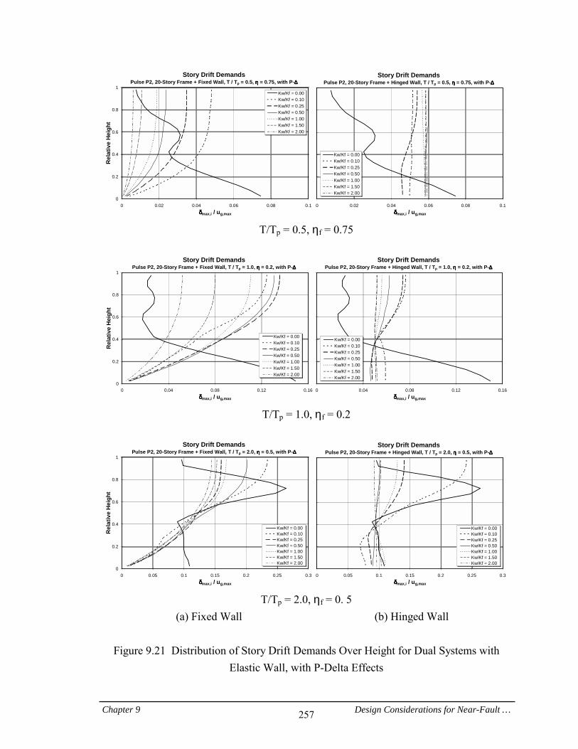
Chapter 9 Design Considerations for Near-Fault … 257
Story Drift DemandsPulse P2, 20-Story Frame + Fixed Wall, T / Tp = 0.5, ηηηη = 0.75, with P-∆∆∆∆
0
0.2
0.4
0.6
0.8
1
0 0.02 0.04 0.06 0.08 0.1δδδδmax,i / ug,max
Rel
ativ
e H
eigh
t
Kw/Kf = 0.00Kw/Kf = 0.10Kw/Kf = 0.25Kw/Kf = 0.50Kw/Kf = 1.00Kw/Kf = 1.50Kw/Kf = 2.00
Story Drift DemandsPulse P2, 20-Story Frame + Hinged Wall, T / Tp = 0.5, ηηηη = 0.75, with P-∆∆∆∆
0 0.02 0.04 0.06 0.08 0.1δδδδmax,i / ug,max
Kw/Kf = 0.00Kw/Kf = 0.10Kw/Kf = 0.25Kw/Kf = 0.50Kw/Kf = 1.00Kw/Kf = 1.50Kw/Kf = 2.00
T/Tp = 0.5, ηf = 0.75
Story Drift Demands
Pulse P2, 20-Story Frame + Fixed Wall, T / Tp = 1.0, ηηηη = 0.2, with P-∆∆∆∆
0
0.2
0.4
0.6
0.8
1
0 0.04 0.08 0.12 0.16δδδδmax,i / ug,max
Rel
ativ
e H
eigh
t
Kw/Kf = 0.00Kw/Kf = 0.10Kw/Kf = 0.25Kw/Kf = 0.50Kw/Kf = 1.00Kw/Kf = 1.50Kw/Kf = 2.00
Story Drift DemandsPulse P2, 20-Story Frame + Hinged Wall, T / Tp = 1.0, ηηηη = 0.2, with P-∆∆∆∆
0 0.04 0.08 0.12 0.16δδδδmax,i / ug,max
Kw/Kf = 0.00Kw/Kf = 0.10Kw/Kf = 0.25Kw/Kf = 0.50Kw/Kf = 1.00Kw/Kf = 1.50Kw/Kf = 2.00
T/Tp = 1.0, ηf = 0.2
Story Drift Demands
Pulse P2, 20-Story Frame + Fixed Wall, T / Tp = 2.0, ηηηη = 0.5, with P-∆∆∆∆
0
0.2
0.4
0.6
0.8
1
0 0.05 0.1 0.15 0.2 0.25 0.3δδδδmax,i / ug,max
Rel
ativ
e H
eigh
t
Kw/Kf = 0.00Kw/Kf = 0.10Kw/Kf = 0.25Kw/Kf = 0.50Kw/Kf = 1.00Kw/Kf = 1.50Kw/Kf = 2.00
Story Drift DemandsPulse P2, 20-Story Frame + Hinged Wall, T / Tp = 2.0, ηηηη = 0.5, with P-∆∆∆∆
0 0.05 0.1 0.15 0.2 0.25 0.3δδδδmax,i / ug,max
Kw/Kf = 0.00Kw/Kf = 0.10Kw/Kf = 0.25Kw/Kf = 0.50Kw/Kf = 1.00Kw/Kf = 1.50Kw/Kf = 2.00
T/Tp = 2.0, ηf = 0. 5
(a) Fixed Wall (b) Hinged Wall
Figure 9.21 Distribution of Story Drift Demands Over Height for Dual Systems with Elastic Wall, with P-Delta Effects
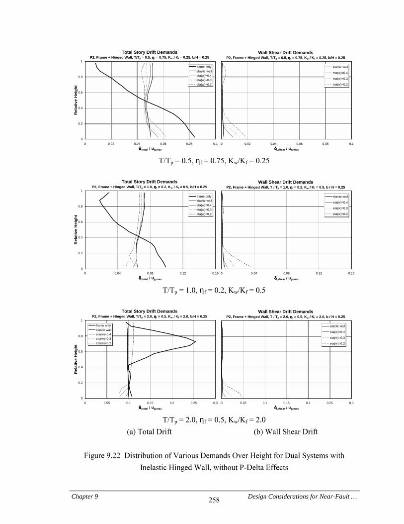
Chapter 9 Design Considerations for Near-Fault … 258
Total Story Drift DemandsP2, Frame + Hinged Wall, T/Tp = 0.5, ηηηηf = 0.75, Kw / Kf = 0.25, b/H = 0.25
0
0.2
0.4
0.6
0.8
1
0 0.02 0.04 0.06 0.08 0.1δδδδi,total / ug,max
Rel
ativ
e H
eigh
t
frame onlyelastic walleta(w)=0.4eta(w)=0.3eta(w)=0.2
Wall Shear Drift DemandsP2, Frame + Hinged Wall, T/Tp = 0.5, ηηηηf = 0.75, Kw / Kf = 0.25, b/H = 0.25
0 0.02 0.04 0.06 0.08 0.1δδδδi,shear / ug,max
elastic wall
eta(w)=0.4
eta(w)=0.3
eta(w)=0.2
T/Tp = 0.5, ηf = 0.75, Kw/Kf = 0.25
Total Story Drift Demands
P2, Frame + Hinged Wall, T/Tp = 1.0, ηηηηf = 0.2, Kw / Kf = 0.5, b/H = 0.25
0
0.2
0.4
0.6
0.8
1
0 0.04 0.08 0.12 0.16δδδδi,total / ug,max
Rel
ativ
e H
eigh
t
frame onlyelastic walleta(w)=0.4eta(w)=0.3eta(w)=0.2
Wall Shear Drift DemandsP2, Frame + Hinged Wall, T / Tp = 1.0, ηηηηf = 0.2, Kw / Kf = 0.5, b / H = 0.25
0 0.04 0.08 0.12 0.16δδδδi,shear / ug,max
elastic wall
eta(w)=0.4
eta(w)=0.3
eta(w)=0.2
T/Tp = 1.0, ηf = 0.2, Kw/Kf = 0.5
Total Story Drift Demands
P2, Frame + Hinged Wall, T/Tp = 2.0, ηηηηf = 0.5, Kw / Kf = 2.0, b/H = 0.25
0
0.2
0.4
0.6
0.8
1
0 0.05 0.1 0.15 0.2 0.25 0.3δδδδi,total / ug,max
Rel
ativ
e H
eigh
t
frame onlyelastic walleta(w)=0.4eta(w)=0.3eta(w)=0.2
Wall Shear Drift DemandsP2, Frame + Hinged Wall, T / Tp = 2.0, ηηηηf = 0.5, Kw / Kf = 2.0, b / H = 0.25
0 0.05 0.1 0.15 0.2 0.25 0.3δδδδi,shear / ug,max
elastic wall
eta(w)=0.4
eta(w)=0.3
eta(w)=0.2
T/Tp = 2.0, ηf = 0.5, Kw/Kf = 2.0
(a) Total Drift (b) Wall Shear Drift
Figure 9.22 Distribution of Various Demands Over Height for Dual Systems with Inelastic Hinged Wall, without P-Delta Effects
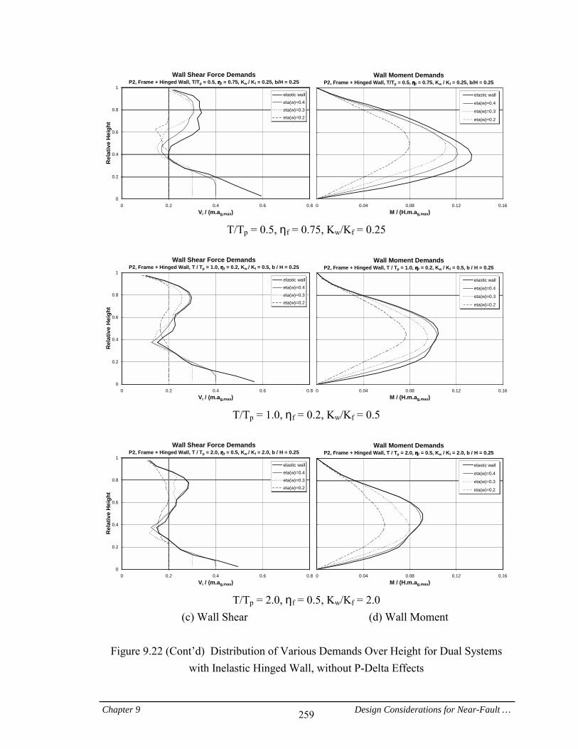
Chapter 9 Design Considerations for Near-Fault … 259
Wall Shear Force DemandsP2, Frame + Hinged Wall, T/Tp = 0.5, ηηηηf = 0.75, Kw / Kf = 0.25, b/H = 0.25
0
0.2
0.4
0.6
0.8
1
0 0.2 0.4 0.6 0.8Vi / (m.ag,max)
Rel
ativ
e H
eigh
t
elastic walleta(w)=0.4eta(w)=0.3eta(w)=0.2
Wall Moment DemandsP2, Frame + Hinged Wall, T/Tp = 0.5, ηηηηf = 0.75, Kw / Kf = 0.25, b/H = 0.25
0 0.04 0.08 0.12 0.16M / (H.m.ag,max)
elastic wall
eta(w)=0.4
eta(w)=0.3
eta(w)=0.2
T/Tp = 0.5, ηf = 0.75, Kw/Kf = 0.25
Wall Shear Force Demands
P2, Frame + Hinged Wall, T / Tp = 1.0, ηηηηf = 0.2, Kw / Kf = 0.5, b / H = 0.25
0
0.2
0.4
0.6
0.8
1
0 0.2 0.4 0.6 0.8Vi / (m.ag,max)
Rel
ativ
e H
eigh
t
elastic walleta(w)=0.4eta(w)=0.3eta(w)=0.2
Wall Moment DemandsP2, Frame + Hinged Wall, T / Tp = 1.0, ηηηηf = 0.2, Kw / Kf = 0.5, b / H = 0.25
0 0.04 0.08 0.12 0.16M / (H.m.ag,max)
elastic wall
eta(w)=0.4
eta(w)=0.3
eta(w)=0.2
T/Tp = 1.0, ηf = 0.2, Kw/Kf = 0.5
Wall Shear Force Demands
P2, Frame + Hinged Wall, T / Tp = 2.0, ηηηηf = 0.5, Kw / Kf = 2.0, b / H = 0.25
0
0.2
0.4
0.6
0.8
1
0 0.2 0.4 0.6 0.8Vi / (m.ag,max)
Rel
ativ
e H
eigh
t
elastic walleta(w)=0.4eta(w)=0.3eta(w)=0.2
Wall Moment DemandsP2, Frame + Hinged Wall, T / Tp = 2.0, ηηηηf = 0.5, Kw / Kf = 2.0, b / H = 0.25
0 0.04 0.08 0.12 0.16M / (H.m.ag,max)
elastic wall
eta(w)=0.4
eta(w)=0.3
eta(w)=0.2
T/Tp = 2.0, ηf = 0.5, Kw/Kf = 2.0
(c) Wall Shear (d) Wall Moment
Figure 9.22 (Cont’d) Distribution of Various Demands Over Height for Dual Systems with Inelastic Hinged Wall, without P-Delta Effects
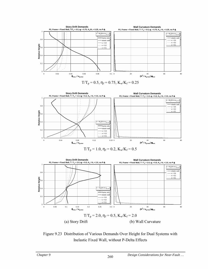
Chapter 9 Design Considerations for Near-Fault … 260
Story Drift DemandsP2, Frame + Fixed Wall, T/Tp = 0.5, ηηηηf = 0.75, Kw/Kf = 0.25, no P-∆∆∆∆
0
0.2
0.4
0.6
0.8
1
0 0.02 0.04 0.06 0.08 0.1δδδδmax,i / ug,max
Rel
ativ
e H
eigh
tframe onlyelastic wallκ===0.4κ===0.2κ===0.1
κ = My/(H.m.ag,max)
Wall Curvature DemandsP2, Frame + Fixed Wall, T / Tp = 0.5, ηηηηf = 0.75, Kw / Kf = 0.25, no P-∆∆∆∆
0 20 40 60 80(H2 / ug,max)====φφφφmax
elastic wallκ===0.4κ===0.2κ===0.1
κ = My/(H.m.ag,max)
T/Tp = 0.5, ηf = 0.75, Kw/Kf = 0.25
Story Drift Demands
P2, Frame + Fixed Wall, T / Tp = 1.0, ηηηηf = 0.2, Kw / Kf = 0.5, no P-∆∆∆∆
0
0.2
0.4
0.6
0.8
1
0 0.04 0.08 0.12 0.16δδδδmax,i / ug,max
Rel
ativ
e H
eigh
t
frame onlyelastic wallκ===0.4κ===0.2κ===0.1
κ = My/(H.m.ag,max)
Wall Curvature DemandsP2, Frame + Fixed Wall, T / Tp = 1.0, ηηηηf = 0.2, Kw / Kf = 0.5, no P-∆∆∆∆
0 20 40 60 80(H2 / ug,max)====φφφφmax
elastic wallκ===0.4κ===0.2κ===0.1
κ = My/(H.m.ag,max)
T/Tp = 1.0, ηf = 0.2, Kw/Kf = 0.5
Story Drift Demands
P2, Frame + Fixed Wall, T / Tp = 2.0, ηηηηf = 0.5, Kw / Kf = 2.0, no P-∆∆∆∆
0
0.2
0.4
0.6
0.8
1
0 0.05 0.1 0.15 0.2 0.25 0.3δδδδmax,i / ug,max
Rel
ativ
e H
eigh
t
frame onlyelastic wallκ===0.4κ===0.2κ===0.1
κ = My/(H.m.ag,max)
Wall Curvature DemandsP2, Frame + Fixed Wall, T / Tp = 2.0, ηηηηf = 0.5, Kw / Kf = 2.0, no P-∆∆∆∆
0 20 40 60 80(H2 / ug,max)====φφφφmax
elastic wallκ===0.4κ===0.2κ===0.1
κ = My/(H.m.ag,max)
T/Tp = 2.0, ηf = 0.5, Kw/Kf = 2.0
(a) Story Drift (b) Wall Curvature
Figure 9.23 Distribution of Various Demands Over Height for Dual Systems with Inelastic Fixed Wall, without P-Delta Effects
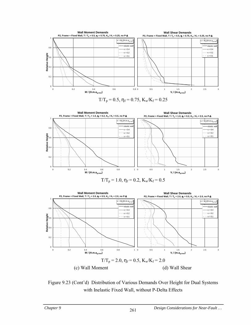
Chapter 9 Design Considerations for Near-Fault … 261
Wall Moment DemandsP2, Frame + Fixed Wall, T / Tp = 0.5, ηηηηf = 0.75, Kw / Kf = 0.25, no P-∆∆∆∆
0
0.2
0.4
0.6
0.8
1
0 0.2 0.4 0.6 0.8M / (H.m.ag,max)
Rel
ativ
e H
eigh
telastic wall
κ===0.4
κ===0.2
κ===0.1
κ = My/(H.m.ag,max)
Wall Shear DemandsP2, Frame + Fixed Wall, T / Tp = 0.5, ηηηηf = 0.75, Kw / Kf = 0.25, no P-∆∆∆∆
0 0.5 1 1.5 2 2.5 3Vi / (m.ag,max)
elastic wallκ===0.4
κ===0.2
κ===0.1
κ = My/(H.m.ag,max)
T/Tp = 0.5, ηf = 0.75, Kw/Kf = 0.25
Wall Moment Demands
P2, Frame + Fixed Wall, T / Tp = 1.0, ηηηηf = 0.2, Kw / Kf = 0.5, no P-∆∆∆∆
0
0.2
0.4
0.6
0.8
1
0 0.2 0.4 0.6 0.8 1M / (H.m.ag,max)
Rel
ativ
e H
eigh
t
elastic wall
κ===0.4
κ===0.2
κ===0.1
κ = My/(H.m.ag,max)
Wall Shear DemandsP2, Frame + Fixed Wall, T / Tp = 1.0, ηηηηf = 0.2, Kw / Kf = 0.5, no P-∆∆∆∆
0 0.5 1 1.5 2 2.5 3Vi / (m.ag,max)
elastic wallκ===0.4
κ===0.2
κ===0.1
κ = My/(H.m.ag,max)
T/Tp = 1.0, ηf = 0.2, Kw/Kf = 0.5
Wall Moment Demands
P2, Frame + Fixed Wall, T / Tp = 2.0, ηηηηf = 0.5, Kw / Kf = 2.0, no P-∆∆∆∆
0
0.2
0.4
0.6
0.8
1
0 0.2 0.4 0.6 0.8 1M / (H.m.ag,max)
Rel
ativ
e H
eigh
t
elastic wall
κ===0.4
κ===0.2
κ===0.1
κ = My/(H.m.ag,max)
Wall Shear DemandsP2, Frame + Fixed Wall, T / Tp = 2.0, ηηηηf = 0.5, Kw / Kf = 2.0, no P-∆∆∆∆
0 0.5 1 1.5 2 2.5 3Vi / (m.ag,max)
elastic wallκ===0.4
κ===0.2
κ===0.1
κ = My/(H.m.ag,max)
T/Tp = 2.0, ηf = 0.5, Kw/Kf = 2.0
(c) Wall Moment (d) Wall Shear
Figure 9.23 (Cont’d) Distribution of Various Demands Over Height for Dual Systems with Inelastic Fixed Wall, without P-Delta Effects
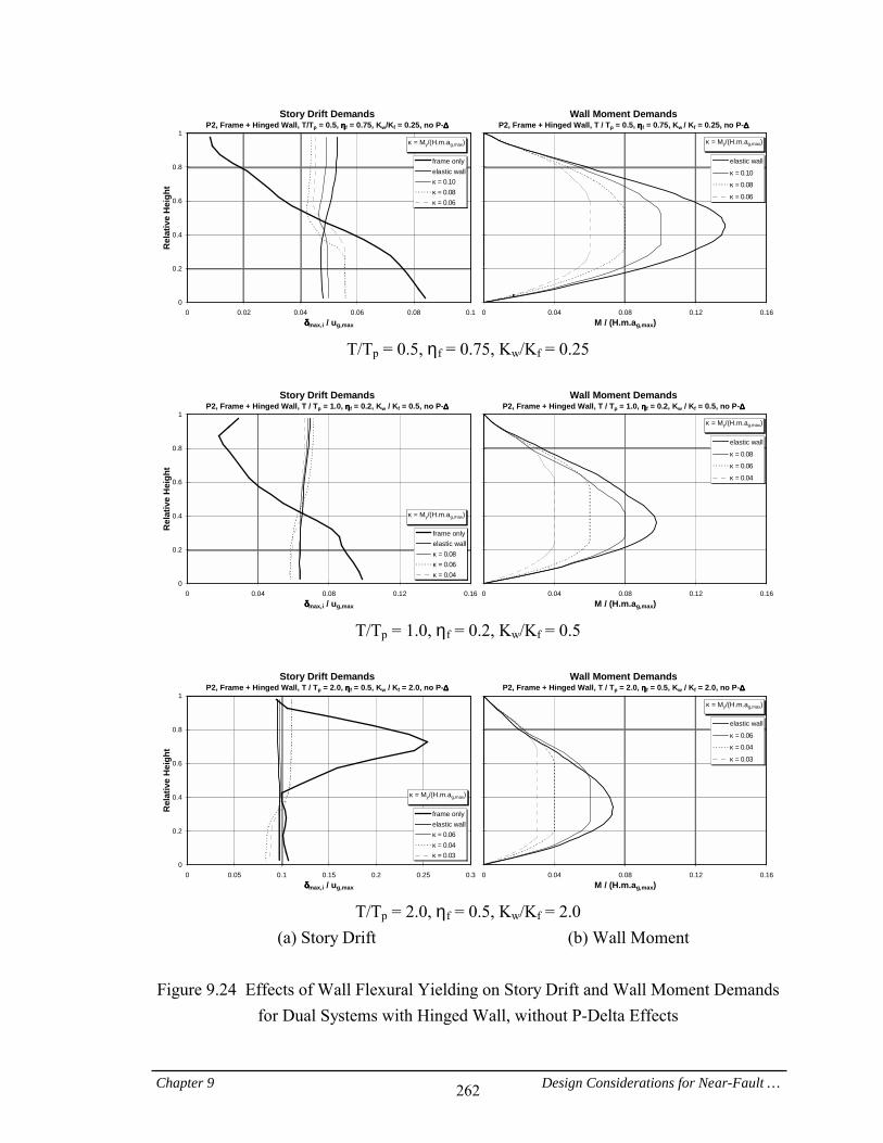
Chapter 9 Design Considerations for Near-Fault … 262
Story Drift DemandsP2, Frame + Hinged Wall, T/Tp = 0.5, ηηηηf = 0.75, Kw/Kf = 0.25, no P-∆∆∆∆
0
0.2
0.4
0.6
0.8
1
0 0.02 0.04 0.06 0.08 0.1δδδδmax,i / ug,max
Rel
ativ
e H
eigh
tframe onlyelastic wallκ===0.10κ===0.08κ===0.06
κ = My/(H.m.ag,max)
Wall Moment DemandsP2, Frame + Hinged Wall, T / Tp = 0.5, ηηηηf = 0.75, Kw / Kf = 0.25, no P-∆∆∆∆
0 0.04 0.08 0.12 0.16M / (H.m.ag,max)
elastic wall
κ===0.10
κ===0.08
κ===0.06
κ = My/(H.m.ag,max)
T/Tp = 0.5, ηf = 0.75, Kw/Kf = 0.25
Story Drift Demands
P2, Frame + Hinged Wall, T / Tp = 1.0, ηηηηf = 0.2, Kw / Kf = 0.5, no P-∆∆∆∆
0
0.2
0.4
0.6
0.8
1
0 0.04 0.08 0.12 0.16δδδδmax,i / ug,max
Rel
ativ
e H
eigh
t
frame onlyelastic wallκ===0.08κ===0.06κ===0.04
κ = My/(H.m.ag,max)
Wall Moment DemandsP2, Frame + Hinged Wall, T / Tp = 1.0, ηηηηf = 0.2, Kw / Kf = 0.5, no P-∆∆∆∆
0 0.04 0.08 0.12 0.16M / (H.m.ag,max)
elastic wall
κ===0.08
κ===0.06
κ===0.04
κ = My/(H.m.ag,max)
T/Tp = 1.0, ηf = 0.2, Kw/Kf = 0.5
Story Drift Demands
P2, Frame + Hinged Wall, T / Tp = 2.0, ηηηηf = 0.5, Kw / Kf = 2.0, no P-∆∆∆∆
0
0.2
0.4
0.6
0.8
1
0 0.05 0.1 0.15 0.2 0.25 0.3δδδδmax,i / ug,max
Rel
ativ
e H
eigh
t
frame onlyelastic wallκ===0.06κ===0.04κ===0.03
κ = My/(H.m.ag,max)
Wall Moment DemandsP2, Frame + Hinged Wall, T / Tp = 2.0, ηηηηf = 0.5, Kw / Kf = 2.0, no P-∆∆∆∆
0 0.04 0.08 0.12 0.16M / (H.m.ag,max)
elastic wall
κ===0.06
κ===0.04
κ===0.03
κ = My/(H.m.ag,max)
T/Tp = 2.0, ηf = 0.5, Kw/Kf = 2.0
(a) Story Drift (b) Wall Moment
Figure 9.24 Effects of Wall Flexural Yielding on Story Drift and Wall Moment Demands for Dual Systems with Hinged Wall, without P-Delta Effects
Chapter 10 Near-Fault Ground Motions from Moderate … 263
CHAPTER 10
NEAR-FAULT GROUND MOTIONS FROM MODERATE EARTHQUAKES
The results of the studies presented in the previous chapters demonstrated the pulse-type characteristics of near-fault ground motions with forward directivity, recorded during relatively large earthquakes with magnitudes ranging from 6.2 to 7.4. The properties of simple pulses were employed to represent such ground motions in Chapter 7, and the pulse representation was taken advantage of in Chapter 9 to study the beneficial effects of strengthening frame structures. An issue that remains to be addressed is whether near-fault ground motions recorded in the forward directivity region of smaller events also exhibit pulse-type characteristics. The results presented in this chapter shed light on the response of SDOF and MDOF structures located in the near-fault region of moderate earthquakes. These earthquakes may not be severe enough to raise a major concern about collapse safety, but they occur more frequently and can endanger the serviceability of the structure or contribute to cumulative damage. Performance-based engineering guidelines require that the behavior of structures subjected to moderate (but more frequent) ground motions also be evaluated. Several near-fault ground motions from moderate events are introduced for this purpose, and their elastic response spectra are investigated. The spectral shapes of near-fault ground motions from moderate events are compared with those of “ordinary” ground motions. Finally, MDOF demands for frame structures subjected to the ground motion records are quantified. 10.1. Ground Motion Records Used in this Study Five near-fault ground motions recorded during the Parkfield (1966) and Coyote Lake (1979) earthquakes are used in the study of moderate events. The designation and basic
Chapter 10 Near-Fault Ground Motions from Moderate … 264
properties of these ground motions are listed in Table 10.1. All five recording stations are located in the forward direction of the corresponding seismic sources. Two horizontal components of each ground motion are obtained from the PEER Strong Motion Database (Silva, 1999). The ground motions are recorded on USGS soil type C (roughly equivalent to NEHRP soil type D), which is compatible with the soil conditions of the records introduced in Chapter 2 for the study of near-fault effects in larger events. Ground velocity time history traces are presented in Fig. 10.1 for the fault-normal and fault-parallel components of the ground motions. The following observations are made:
• = The time history traces for the Parkfield records do not exhibit typical pulse-type characteristics similar to those observed in Chapter 2 for near-fault records with forward directivity. The maximum time history values for the two components are quite comparable, and there is no dominant component.
• = The Coyote Lake records are more pulse-like in their time histories compared to
the Parkfield records. The fault-parallel component of these records contains a more distinct pulse of motion than the fault-normal component. The PGV values for the fault-parallel component are considerably larger than their fault-normal counterparts.
10.2. Elastic Response Spectra Figure 10.2 illustrates acceleration (elastic strength demand), velocity, and displacement spectra of the near-fault ground motions introduced in the previous section. Each graph shows the spectra for the fault-normal and fault-parallel components. The following observations are made:
• = The spectra of the Parkfield records confirm the observations made from the time history traces. The shape of the spectra is not like that of pulse-type ground motions or near-fault ground motions recorded during large earthquakes. No component of the record dominates in the spectra.
• = For the Coyote Lake ground motions the spectral values for the fault-parallel
component are larger than the values for the fault-normal component, which is contrary to the observation made for near-fault ground motions from large

Chapter 10 Near-Fault Ground Motions from Moderate … 265
earthquakes. Pulse-type characteristics observed in the time histories appear as a global hump in the velocity spectra. However, the humps of the velocity spectra are not as well-defined as those of the spectra of near-fault ground motions recorded during large events (see Chapter 2).
The conclusion is that ground motions recorded in the forward direction of a moderate earthquake may not be characterized by a distinct pulse. The reason may be that the amount of energy released in moderate events is not sufficiently large to cause severe directivity effects. Contrary to near-fault records from large earthquakes, ground motions from moderate earthquakes have comparable fault-normal and fault-parallel components. 10.2.1 Comparison with Ordinary Ground Motions It was demonstrated that near-fault records from moderate events might not contain distinct pulse-type characteristics. The objective of this part of the study is to evaluate the extent to which moderate-magnitude near-fault ground motions can be represented by “ordinary” ground motions that are not affected by directivity in the near-fault region. Individual Ground Motions: The spectra of the ground motions introduced in the previous section are compared with reference spectra derived from an attenuation relationship proposed by Abrahamson and Silva (1997). The attenuation relationship, which expresses the spectral acceleration (Sa [g]) at a specific period as a function of the moment magnitude (Mw) and the closest distance from the site to the rupture plane (R [km]), is given by the following equation for strike-slip faulting:
)(PGAS.f R),(Mf )ln(S rock5w1a += (10.1)
where Sa is spectral acceleration for the average horizontal component, S is a soil factor with its value being zero for rock and shallow soil (Geomatrix A and B) and unity for deep soil (Geomatrix C and D), PGArock is the peak ground acceleration (spectral acceleration at a very short period) from Eq. (10.1) with S = 0, and the functions f1 (for Mw ≤ 6.4) and f5 are given as follows:
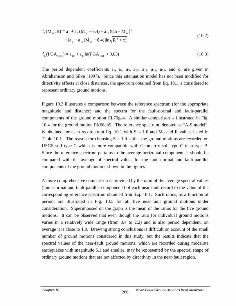
Chapter 10 Near-Fault Ground Motions from Moderate … 266
24
2w133
2w12w21w1
cR)]ln4.6(Ma[a
)M(8.5a)4.6(MaaR),(Mf
+−++
−+−+= (10.2)
)03.0GAPln(aa)(PGAf rock1110rock5 ++= (10.3)
The period dependent coefficients a1, a2, a3, a10, a11, a12, a13, and c4 are given in Abrahamson and Silva (1997). Since this attenuation model has not been modified for directivity effects at close distances, the spectrum obtained from Eq. 10.1 is considered to represent ordinary ground motions. Figure 10.3 illustrates a comparison between the reference spectrum (for the appropriate magnitude and distance) and the spectra for the fault-normal and fault-parallel components of the ground motion CL79ga4. A similar comparison is illustrated in Fig. 10.4 for the ground motion PK66ch5. The reference spectrum, denoted as “A-S model”, is obtained for each record from Eq. 10.1 with S = 1.0 and Mw and R values listed in Table 10.1. The reason for choosing S = 1.0 is that the ground motions are recorded on USGS soil type C which is more compatible with Geomatrix soil type C than type B. Since the reference spectrum pertains to the average horizontal component, it should be compared with the average of spectral values for the fault-normal and fault-parallel components of the ground motions shown in the figures. A more comprehensive comparison is provided by the ratio of the average spectral values (fault-normal and fault-parallel components) of each near-fault record to the value of the corresponding reference spectrum obtained from Eq. 10.1. Such ratios, as a function of period, are illustrated in Fig. 10.5 for all five near-fault ground motions under consideration. Superimposed on the graph is the mean of the ratios for the five ground motions. It can be observed that even though the ratio for individual ground motions varies in a relatively wide range (from 0.4 to 2.2) and is also period dependent, on average it is close to 1.0. Drawing strong conclusions is difficult on account of the small number of ground motions considered in this study, but the results indicate that the spectral values of the near-fault ground motions, which are recorded during moderate earthquakes with magnitude 6.1 and smaller, may be represented by the spectral shape of ordinary ground motions that are not affected by directivity in the near-fault region.

Chapter 10 Near-Fault Ground Motions from Moderate … 267
To provide a comprehensive comparison of the fault-normal and fault-parallel components of near-fault ground motions from moderate events, Fig. 10.6 illustrates the ratio of fault-normal to fault-parallel spectral values as a function of period for the five ground motions. The mean of the ratios for the five ground motions is also shown. It can be observed that the ratio is period and ground motion dependent, but on average it is not far from 1.0 (with values generally smaller than 1.0). As also pointed out previously, this is in contrast to the observations made for near-fault records from large events, in which case the fault-normal component is significantly more severe than the fault-parallel component. Scenario Events: Figure 10.7 compares elastic acceleration spectra for two scenario events with R = 3 km and Mw = 6.0 and 7.0, obtained from two different approaches as follows: (1) using the Abrahamson-Silva attenuation model discussed previously, which does not take directivity effects into consideration, and (2) using the equivalent pulse model discussed in Section 9.1, which takes forward directivity into account. In the first approach, Eqs. 10.1 to 10.3 are utilized with S = 1.0. It should be noted that for Mw > 6.4, the coefficient a2 in Eq. 10.2 is replaced by the coefficient a4 given in Abrahamson and Silva (1997). The values obtained from Eq. 10.1 correspond to the mean acceleration spectrum of the two components. A modification factor proposed by Somerville et al. (1997b) is utilized here in order to convert the mean spectrum to the spectrum corresponding to the fault-normal component. The following equation represents the ratio of fault-normal to average spectral values for Mw ≥ 6: ln(Sa
FN/SaAVG) = C1 + C2 ln(R + 1) + C3 (Mw – 6) (10.4)
where C1, C2, and C3 are period dependent coefficients given in Somerville et al. (1997b). In the second approach, the elastic acceleration spectrum of pulse P2 (see Fig. 5.4) is utilized, along with Eqs. 9.1 and 9.3, to estimate the pulse period (Tp) and intensity (ag,max = 4veff/Tp) of the equivalent pulse for the scenario events. In order to be compatible with the spectrum obtained from the first approach, the pulse spectrum is computed for a 5% damping ratio. Since the fault-normal component of near-fault ground motions with forward directivity was used in developing Eqs. 9.1 and 9.3, the spectral values obtained
Chapter 10 Near-Fault Ground Motions from Moderate … 268
from the equivalent pulse model pertain to the fault-normal component and include directivity effects. The following observations are made from Fig. 10.7:
• = For large earthquakes (Mw = 7.0) the spectral shape of the pulse-type ground motion, which represents near-fault ground motions with forward directivity, differs radically from the spectral shape of ordinary ground motions without directivity effects. In the period range T > 1.0 sec., the spectral values for the pulse-type ground motion are considerably larger than those for ordinary records.
• = For moderate earthquakes (Mw = 6.0) the spectral shapes are much closer,
implying that the directivity effect in the near-fault region of moderate earthquakes is less important than that of large earthquakes. In the period range T > 2.0 sec., the spectral values for the pulse-type ground motion are even smaller than the corresponding values for ordinary records.
These observations further support the hypothesis that spectral values of the near-fault ground motions from moderate earthquakes (Mw ≤ 6) can be represented by the spectral shape of ordinary ground motions not affected by directivity in the near-fault region. 10.3. Story Ductility Demands Over Height To evaluate MDOF demands for structures subjected to near-fault records from moderate earthquakes, distributions of story ductility demands over the height of the structure are presented in this section. Figures 10.8 and 10.9 illustrate the story ductility distributions for fault-normal and fault-parallel components of ground motions CL79ga3 and PK66ch8. The generic 20-story frame introduced in Section 3.2 is utilized here with periods of T = 0.5, 1.0, and 2.0 sec., and base shear strengths defined by the coefficient γ = Vy/W. The following observations can be made:
• = For short period (T = 0.5 sec.) and strong structures, the distribution of story ductility is relatively uniform over the height. For weaker structures the maximum story ductility occurs in the bottom story, and grows rapidly with a decrease in strength. This pattern is not much different from the observations made for near-fault records from large earthquakes (see Chapter 4) and pulse-type ground motions (see Chapter 6).
Chapter 10 Near-Fault Ground Motions from Moderate … 269
• = For long period structures (T = 2.0 sec.) the story ductility distributions for CL79ga3 exhibit some pulse-type patterns, but to a lesser extent compared to records from large events. Similar patterns are observed for both the fault-normal and fault-parallel components. The critical story (with maximum ductility) is in the top portion for relatively strong structures, and migrates to the base when the base shear strength is reduced. The story ductility distributions for PK66ch8 are less pulse-like and show characteristics similar to those of ordinary ground motion. This is in agreement with the observations previously made from the spectra and time history traces.
• = For a given base shear strength value, larger spectral values of the fault-parallel
component of CL79ga3 translate into larger story ductility demands for this component, especially at T = 0.5 sec.
The conclusion based on the results presented here is that the response of MDOF structures to ground motions recorded in the near-fault region of moderate earthquakes does not exhibit strong pulse-type characteristics. In order to explore the strength dependence of story ductility demands, unrealistically small values for the base shear strength coefficient γ had to be used in the investigations. To put the presented results in perspective, a realistic base shear strength is estimated here based on the design provisions of UBC’97. Assuming that the structure is at a distance of R = 3 km from the source in Seismic Zone 4 (soil type SD), the base shear strength of the structure can be estimated from the UBC design spectrum (including the near-fault factor for Type A sources), considering a strength reduction factor of 8, and an overstrength factor of 2. As shown in Fig. 9.4 (the curve denotes as “UBC/4, with NFF”), the strength coefficients for T = 0.5, 1.0, and 2.0 sec. are γ = 0.39, 0.30, and 0.15, respectively. The results presented in Figs. 10.8 and 10.9 indicate that for these γ values, the structure subjected to the two records under consideration remains elastic or almost elastic. This close to elastic behavior signifies minor structural damage, and indicates that structures subjected to these ground motions are likely to meet standard performance objectives. The conclusion to be drawn is that the near-fault effect diminishes with decreasing magnitude and becomes unimportant for magnitudes of about 6.1 and smaller.
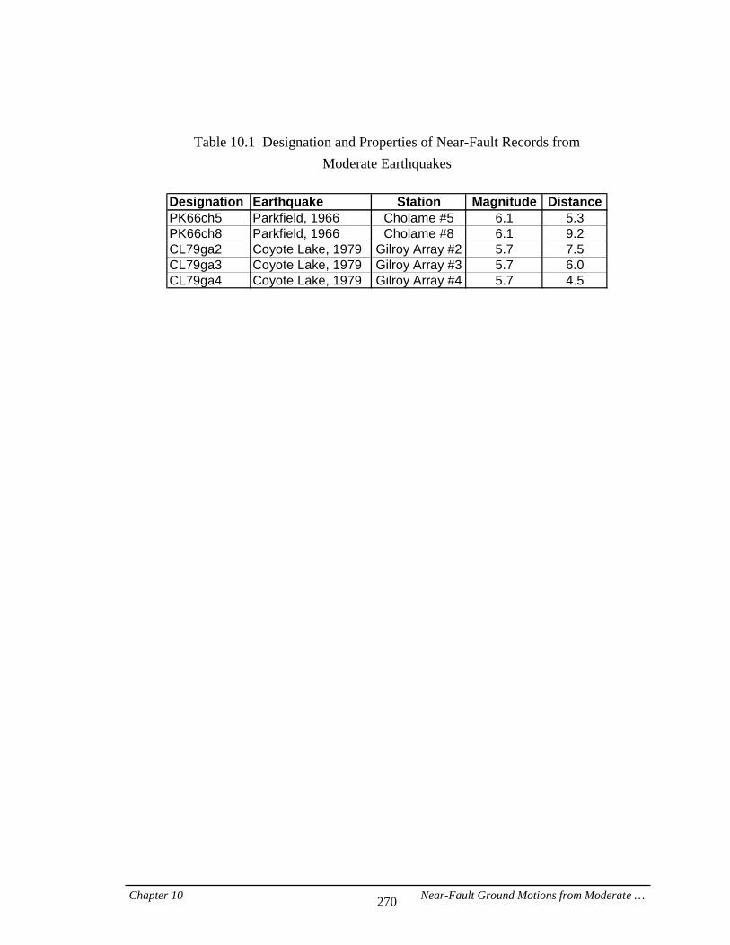
Chapter 10 Near-Fault Ground Motions from Moderate … 270
Table 10.1 Designation and Properties of Near-Fault Records from Moderate Earthquakes
Designation Earthquake Station Magnitude DistancePK66ch5 Parkfield, 1966 Cholame #5 6.1 5.3PK66ch8 Parkfield, 1966 Cholame #8 6.1 9.2CL79ga2 Coyote Lake, 1979 Gilroy Array #2 5.7 7.5CL79ga3 Coyote Lake, 1979 Gilroy Array #3 5.7 6.0CL79ga4 Coyote Lake, 1979 Gilroy Array #4 5.7 4.5
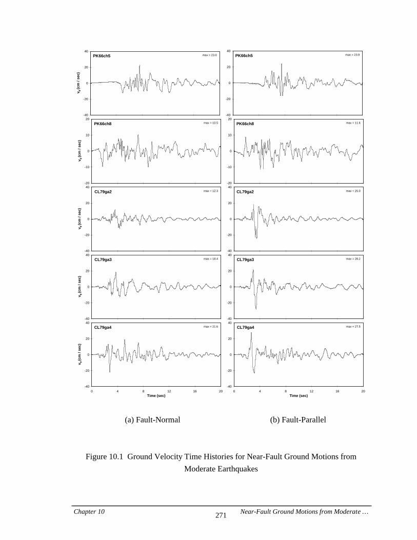
Chapter 10 Near-Fault Ground Motions from Moderate … 271
-40
-20
0
20
40
v g (c
m /
sec)
max = 23.0PK66ch5
-40
-20
0
20
40max = 23.9PK66ch5
-20
-10
0
10
20
v g (c
m /
sec)
max = 10.5PK66ch8
-20
-10
0
10
20max = 11.6PK66ch8
-40
-20
0
20
40
v g (c
m /
sec)
max = 12.3CL79ga2
-40
-20
0
20
40max = 25.0CL79ga2
-40
-20
0
20
40
v g (c
m /
sec)
max = 18.4CL79ga3
-40
-20
0
20
40max = 28.2CL79ga3
-40
-20
0
20
40
0 4 8 12 16 20Time (sec)
v g (c
m /
sec)
max = 21.6CL79ga4
-40
-20
0
20
40
0 4 8 12 16 20Time (sec)
max = 27.5CL79ga4
(a) Fault-Normal (b) Fault-Parallel
Figure 10.1 Ground Velocity Time Histories for Near-Fault Ground Motions from Moderate Earthquakes
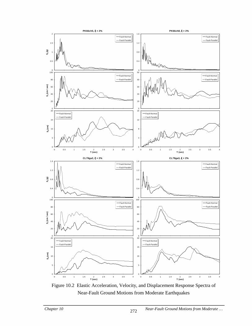
Chapter 10 Near-Fault Ground Motions from Moderate … 272
PK66ch5, ξξξξ = 2%
0
0.5
1
1.5
2
S a (g
)
Fault-Normal
Fault-Parallel
PK66ch8, ξξξξ = 2%
0
0.4
0.8
1.2
1.6Fault-Normal
Fault-Parallel
0
20
40
60
80
100
S v (c
m /
sec)
Fault-Normal
Fault-Parallel
0
10
20
30
40
50
Fault-Normal
Fault-Parallel
0
5
10
15
20
0 0.5 1 1.5 2 2.5 3 3.5 4T (sec)
S d (c
m)
Fault-Normal
Fault-Parallel
0
4
8
12
16
0 0.5 1 1.5 2 2.5 3 3.5 4T (sec)
Fault-Normal
Fault-Parallel
CL79ga2, ξξξξ = 2%
0
0.4
0.8
1.2
1.6
S a (g
)
Fault-Normal
Fault-Parallel
CL79ga3, ξξξξ = 2%
0
0.4
0.8
1.2
1.6Fault-Normal
Fault-Parallel
0
20
40
60
80
100
S v (c
m /
sec)
Fault-Normal
Fault-Parallel
0
20
40
60
80
100
Fault-Normal
Fault-Parallel
0
5
10
15
20
0 0.5 1 1.5 2 2.5 3 3.5 4T (sec)
S d (c
m)
Fault-Normal
Fault-Parallel
0
5
10
15
20
0 0.5 1 1.5 2 2.5 3 3.5 4T (sec)
Fault-Normal
Fault-Parallel
Figure 10.2 Elastic Acceleration, Velocity, and Displacement Response Spectra of
Near-Fault Ground Motions from Moderate Earthquakes
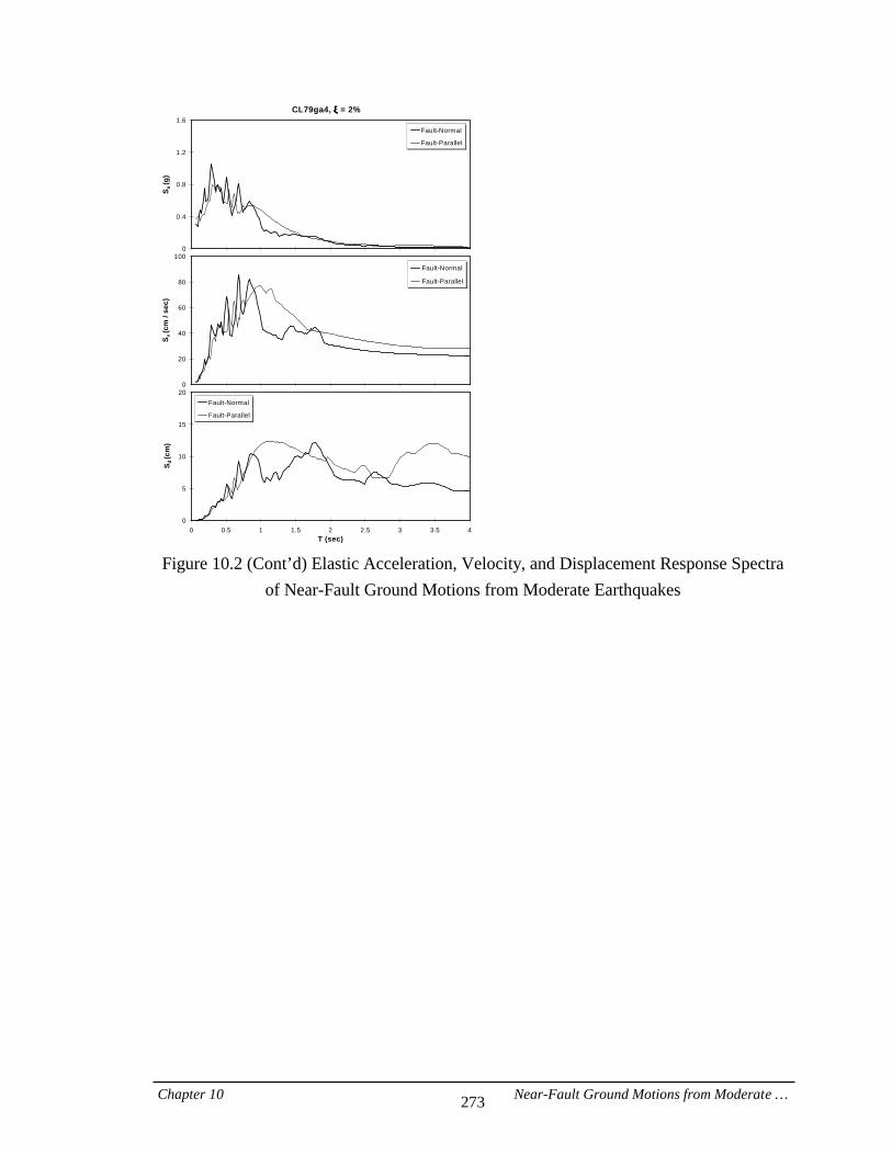
Chapter 10 Near-Fault Ground Motions from Moderate … 273
CL79ga4, ξξξξ = 2%
0
0.4
0.8
1.2
1.6
S a (g
)
Fault-Normal
Fault-Parallel
0
20
40
60
80
100
S v (c
m /
sec)
Fault-Normal
Fault-Parallel
0
5
10
15
20
0 0.5 1 1.5 2 2.5 3 3.5 4T (sec)
S d (c
m)
Fault-Normal
Fault-Parallel
Figure 10.2 (Cont’d) Elastic Acceleration, Velocity, and Displacement Response Spectra
of Near-Fault Ground Motions from Moderate Earthquakes
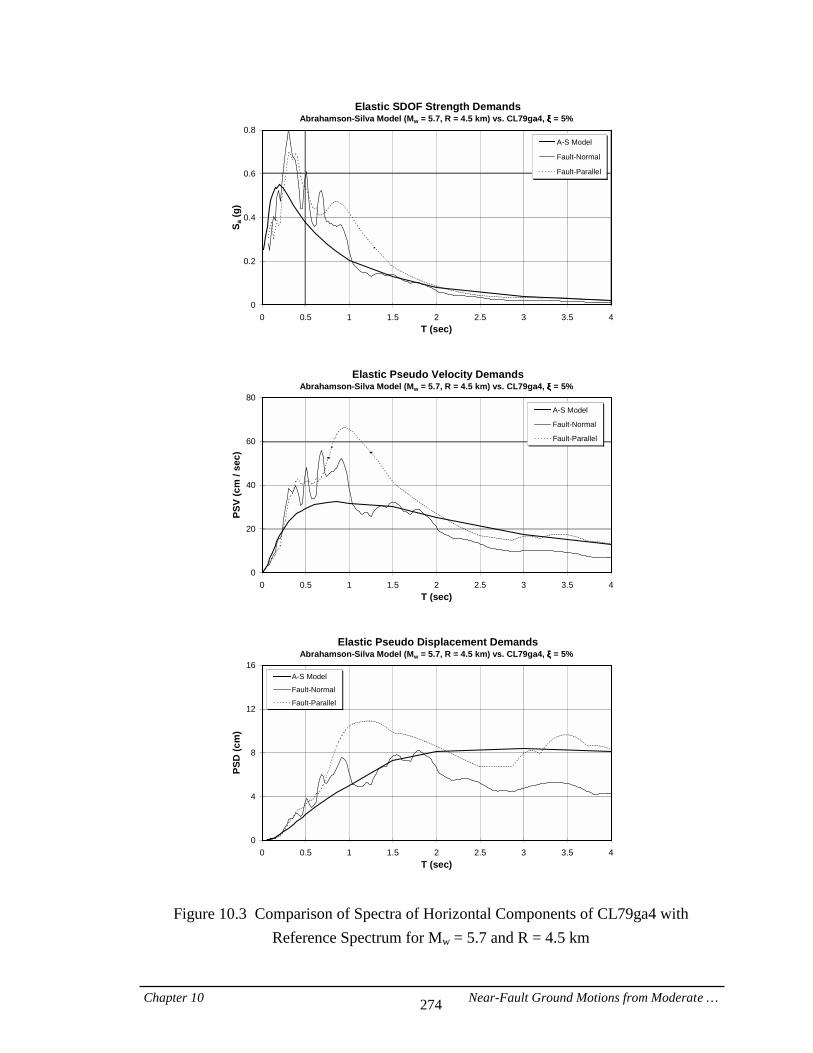
Chapter 10 Near-Fault Ground Motions from Moderate … 274
Elastic SDOF Strength DemandsAbrahamson-Silva Model (Mw = 5.7, R = 4.5 km) vs. CL79ga4, ξξξξ = 5%
0
0.2
0.4
0.6
0.8
0 0.5 1 1.5 2 2.5 3 3.5 4T (sec)
S a (g
)
A-S Model
Fault-Normal
Fault-Parallel
Elastic Pseudo Velocity DemandsAbrahamson-Silva Model (Mw = 5.7, R = 4.5 km) vs. CL79ga4, ξξξξ = 5%
0
20
40
60
80
0 0.5 1 1.5 2 2.5 3 3.5 4T (sec)
PSV
(cm
/ se
c)
A-S Model
Fault-Normal
Fault-Parallel
Elastic Pseudo Displacement DemandsAbrahamson-Silva Model (Mw = 5.7, R = 4.5 km) vs. CL79ga4, ξξξξ = 5%
0
4
8
12
16
0 0.5 1 1.5 2 2.5 3 3.5 4T (sec)
PSD
(cm
)
A-S Model
Fault-Normal
Fault-Parallel
Figure 10.3 Comparison of Spectra of Horizontal Components of CL79ga4 with Reference Spectrum for Mw = 5.7 and R = 4.5 km
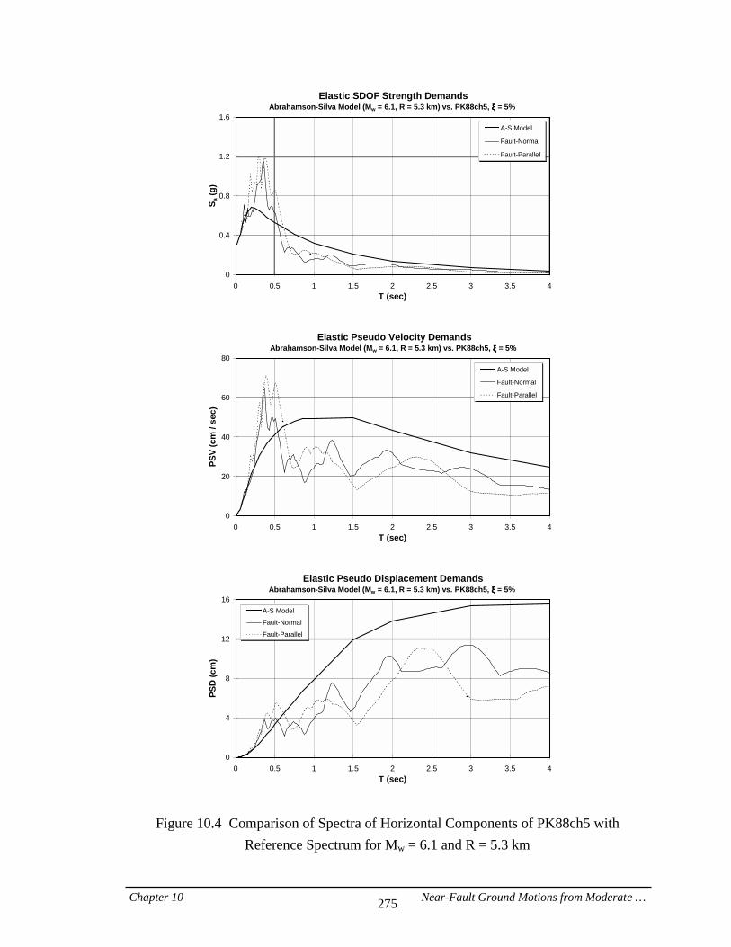
Chapter 10 Near-Fault Ground Motions from Moderate … 275
Elastic SDOF Strength DemandsAbrahamson-Silva Model (Mw = 6.1, R = 5.3 km) vs. PK88ch5, ξξξξ = 5%
0
0.4
0.8
1.2
1.6
0 0.5 1 1.5 2 2.5 3 3.5 4T (sec)
S a (g
)
A-S Model
Fault-Normal
Fault-Parallel
Elastic Pseudo Velocity DemandsAbrahamson-Silva Model (Mw = 6.1, R = 5.3 km) vs. PK88ch5, ξξξξ = 5%
0
20
40
60
80
0 0.5 1 1.5 2 2.5 3 3.5 4T (sec)
PSV
(cm
/ se
c)
A-S Model
Fault-Normal
Fault-Parallel
Elastic Pseudo Displacement DemandsAbrahamson-Silva Model (Mw = 6.1, R = 5.3 km) vs. PK88ch5, ξξξξ = 5%
0
4
8
12
16
0 0.5 1 1.5 2 2.5 3 3.5 4T (sec)
PSD
(cm
)
A-S Model
Fault-Normal
Fault-Parallel
Figure 10.4 Comparison of Spectra of Horizontal Components of PK88ch5 with Reference Spectrum for Mw = 6.1 and R = 5.3 km

Chapter 10 Near-Fault Ground Motions from Moderate … 276
Elastic SDOF Strength Demand RatiosNear-Fault Records vs. Abrahamson-Silva Model, Avg. Comp., ξξξξ = 5%
0
0.5
1
1.5
2
2.5
0 1 2 3 4 5T (sec)
S are
cord
/ SaA
-S m
odel
PK66ch5PK66ch8CL79ga2CL79ga3CL79ga4Average
Figure 10.5 Ratio of Average Spectrum of Components of Near-Fault Records to
Corresponding Reference Spectrum
Elastic SDOF Strength Demand RatiosComparison of Fault-Normal and Fault-Parallel Componets, ξξξξ = 5%
0
0.5
1
1.5
2
2.5
0 1 2 3 4 5T (sec)
S aFN
/ SaFP
PK66ch5PK66ch8CL79ga2CL79ga3CL79ga4Average
Figure 10.6 Ratio of Spectral Values of Fault-Normal to Fault-Parallel Components of
Near-Fault Ground Motions from Moderate Earthquakes
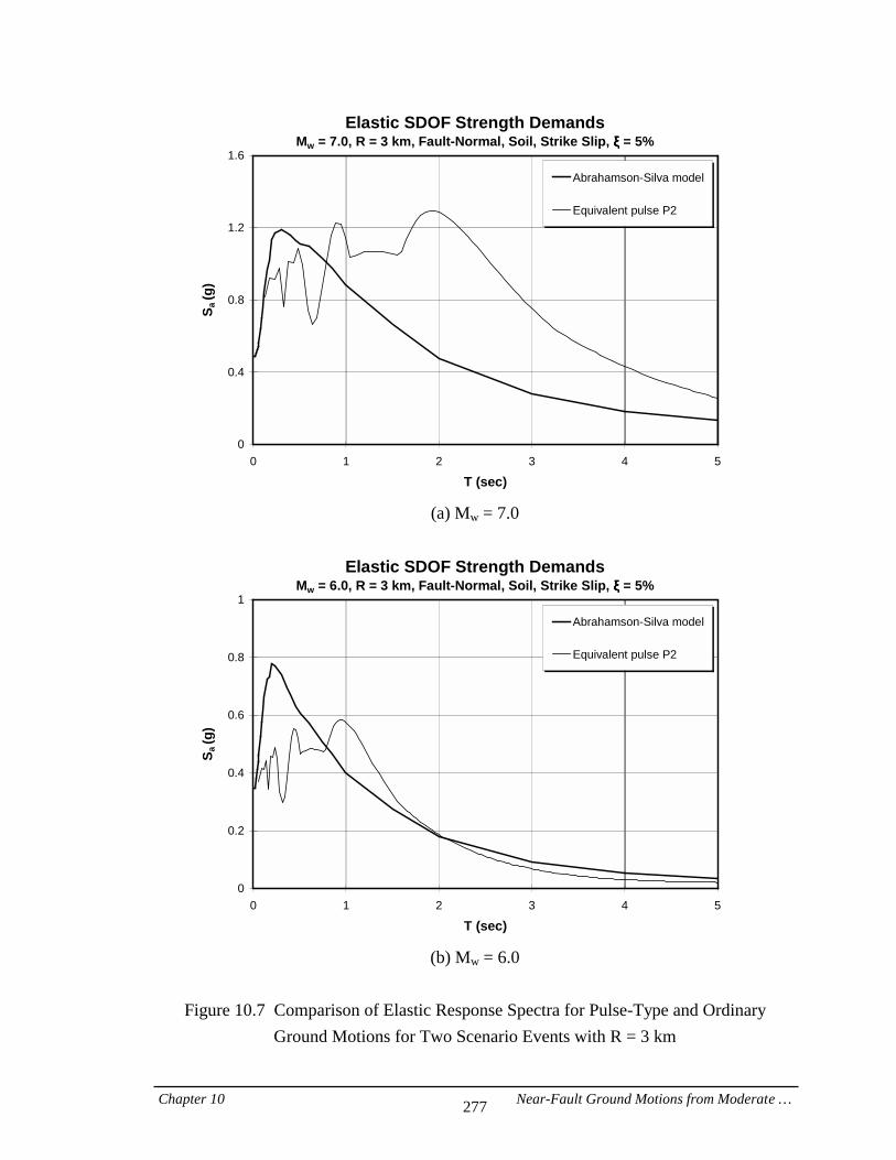
Chapter 10 Near-Fault Ground Motions from Moderate … 277
Elastic SDOF Strength Demands Mw = 7.0, R = 3 km, Fault-Normal, Soil, Strike Slip, ξξξξ===== 5%
0
0.4
0.8
1.2
1.6
0 1 2 3 4 5
T (sec)
S a (g
)
Abrahamson-Silva model
Equivalent pulse P2
(a) Mw = 7.0
Elastic SDOF Strength Demands
Mw = 6.0, R = 3 km, Fault-Normal, Soil, Strike Slip, ξξξξ===== 5%
0
0.2
0.4
0.6
0.8
1
0 1 2 3 4 5
T (sec)
S a (g
)
Abrahamson-Silva model
Equivalent pulse P2
(b) Mw = 6.0
Figure 10.7 Comparison of Elastic Response Spectra for Pulse-Type and Ordinary
Ground Motions for Two Scenario Events with R = 3 km
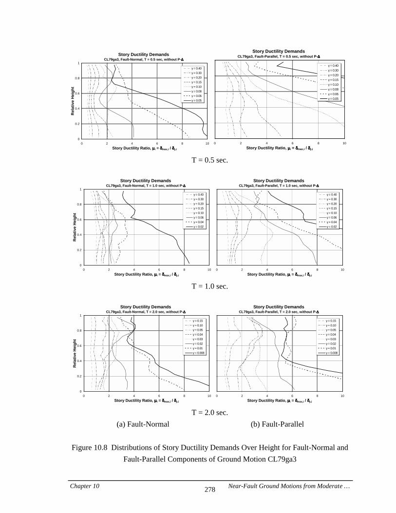
Chapter 10 Near-Fault Ground Motions from Moderate … 278
Story Ductility DemandsCL79ga3, Fault-Normal, T = 0.5 sec, without P-∆∆∆∆
0
0.2
0.4
0.6
0.8
1
0 2 4 6 8 10Story Ductility Ratio, µµµµi = δδδδmax,i / δδδδy,i
Rel
ativ
e H
eigh
tγ===0.40γ===0.30γ===0.20γ===0.15γ===0.10γ===0.08γ===0.06γ===0.05
Story Ductility DemandsCL79ga3, Fault-Parallel, T = 0.5 sec, without P-∆∆∆∆
0 2 4 6 8 10Story Ductility Ratio, µµµµi = δδδδmax,i / δδδδy,i
γ===0.40γ===0.30γ===0.20γ===0.15γ===0.10γ===0.08γ===0.06γ===0.05
T = 0.5 sec.
Story Ductility Demands
CL79ga3, Fault-Normal, T = 1.0 sec, without P-∆∆∆∆
0
0.2
0.4
0.6
0.8
1
0 2 4 6 8 10Story Ductility Ratio, µµµµi = δδδδmax,i / δδδδy,i
Rel
ativ
e H
eigh
t
γ===0.40γ===0.30γ===0.20γ===0.15γ===0.10γ===0.06γ===0.04γ===0.02
Story Ductility DemandsCL79ga3, Fault-Parallel, T = 1.0 sec, without P-∆∆∆∆
0 2 4 6 8 10Story Ductility Ratio, µµµµi = δδδδmax,i / δδδδy,i
γ===0.40γ===0.30γ===0.20γ===0.15γ===0.10γ===0.06γ===0.04γ===0.02
T = 1.0 sec.
Story Ductility Demands
CL79ga3, Fault-Normal, T = 2.0 sec, without P-∆∆∆∆
0
0.2
0.4
0.6
0.8
1
0 2 4 6 8 10Story Ductility Ratio, µµµµi = δδδδmax,i / δδδδy,i
Rel
ativ
e H
eigh
t
γ===0.15γ===0.10γ===0.05γ===0.04γ===0.03γ===0.02γ===0.01γ===0.008
Story Ductility DemandsCL79ga3, Fault-Parallel, T = 2.0 sec, without P-∆∆∆∆
0 2 4 6 8 10Story Ductility Ratio, µµµµi = δδδδmax,i / δδδδy,i
γ===0.15γ===0.10γ===0.05γ===0.04γ===0.03γ===0.02γ===0.01γ===0.008
T = 2.0 sec.
(a) Fault-Normal (b) Fault-Parallel
Figure 10.8 Distributions of Story Ductility Demands Over Height for Fault-Normal and Fault-Parallel Components of Ground Motion CL79ga3
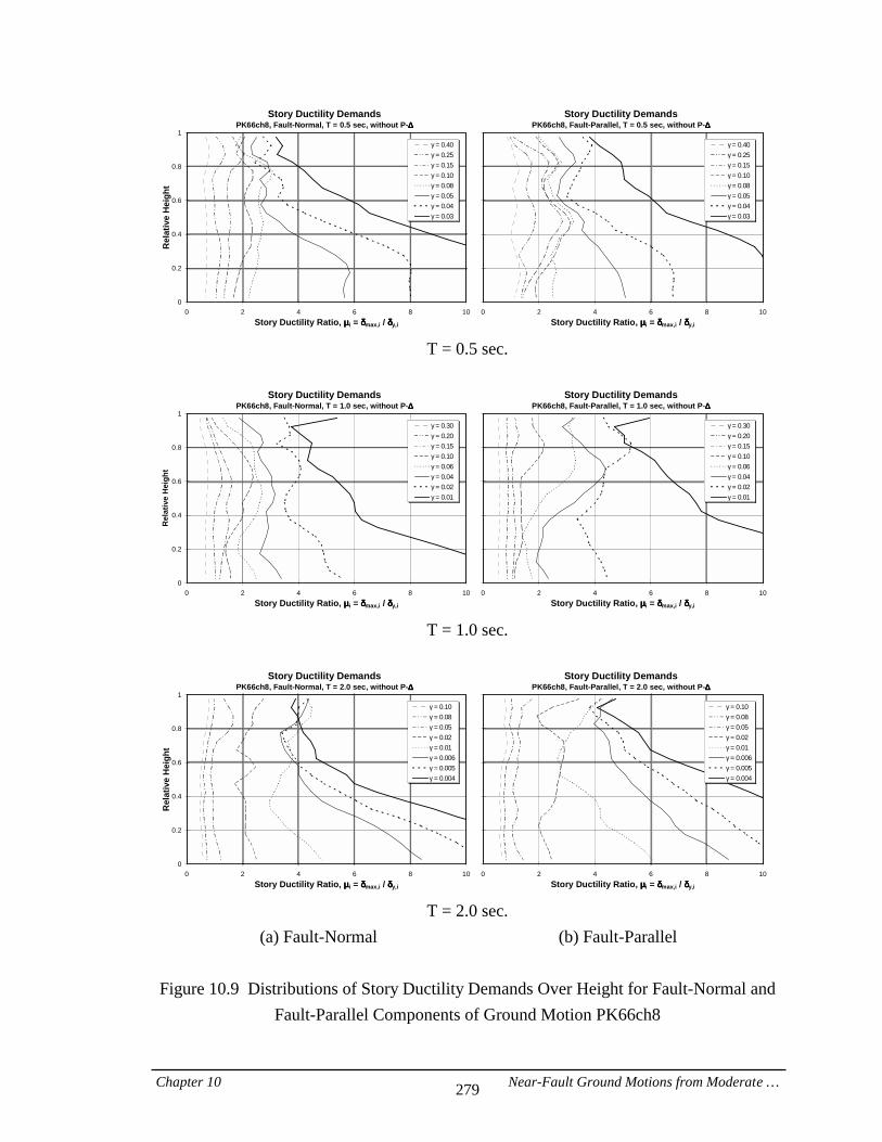
Chapter 10 Near-Fault Ground Motions from Moderate … 279
Story Ductility DemandsPK66ch8, Fault-Normal, T = 0.5 sec, without P-∆∆∆∆
0
0.2
0.4
0.6
0.8
1
0 2 4 6 8 10Story Ductility Ratio, µµµµi = δδδδmax,i / δδδδy,i
Rel
ativ
e H
eigh
t
γ===0.40γ===0.25γ===0.15γ===0.10γ===0.08γ===0.05γ===0.04γ===0.03
Story Ductility DemandsPK66ch8, Fault-Parallel, T = 0.5 sec, without P-∆∆∆∆
0 2 4 6 8 10Story Ductility Ratio, µµµµi = δδδδmax,i / δδδδy,i
γ===0.40γ===0.25γ===0.15γ===0.10γ===0.08γ===0.05γ===0.04γ===0.03
T = 0.5 sec.
Story Ductility Demands
PK66ch8, Fault-Normal, T = 1.0 sec, without P-∆∆∆∆
0
0.2
0.4
0.6
0.8
1
0 2 4 6 8 10Story Ductility Ratio, µµµµi = δδδδmax,i / δδδδy,i
Rel
ativ
e H
eigh
t
γ===0.30γ===0.20γ===0.15γ===0.10γ===0.06γ===0.04γ===0.02γ===0.01
Story Ductility DemandsPK66ch8, Fault-Parallel, T = 1.0 sec, without P-∆∆∆∆
0 2 4 6 8 10Story Ductility Ratio, µµµµi = δδδδmax,i / δδδδy,i
γ===0.30γ===0.20γ===0.15γ===0.10γ===0.06γ===0.04γ===0.02γ===0.01
T = 1.0 sec.
Story Ductility Demands
PK66ch8, Fault-Normal, T = 2.0 sec, without P-∆∆∆∆
0
0.2
0.4
0.6
0.8
1
0 2 4 6 8 10Story Ductility Ratio, µµµµi = δδδδmax,i / δδδδy,i
Rel
ativ
e H
eigh
t
γ===0.10γ===0.08γ===0.05γ===0.02γ===0.01γ===0.006γ===0.005γ===0.004
Story Ductility DemandsPK66ch8, Fault-Parallel, T = 2.0 sec, without P-∆∆∆∆
0 2 4 6 8 10Story Ductility Ratio, µµµµi = δδδδmax,i / δδδδy,i
γ===0.10γ===0.08γ===0.05γ===0.02γ===0.01γ===0.006γ===0.005γ===0.004
T = 2.0 sec.
(a) Fault-Normal (b) Fault-Parallel
Figure 10.9 Distributions of Story Ductility Demands Over Height for Fault-Normal and Fault-Parallel Components of Ground Motion PK66ch8
Chapter 11 Summary and Conclusions 280
CHAPTER 11
SUMMARY AND CONCLUSIONS
The major objective of the study presented in this report is to develop a basic understanding of the important attributes that characterize near-fault ground motions and their effects on the response of elastic and inelastic SDOF and MDOF structural systems. It is necessary to identify the response characteristics that set near-fault ground motions apart from “ordinary” ground motions whose effects on the response of structures have been considered, either explicitly or implicitly, in presently employed design procedures. A comprehensive evaluation of seismic demands is presented for SDOF systems and MDOF frame structures subjected to near-fault and pulse-type ground motions. The SDOF systems employed in this study have bilinear hysteretic characteristics. A generic 20-story frame model is used extensively to evaluate MDOF response characteristics of frame structures. This frame model is designed according to the “weak beam – strong column” concept, and member strengths are tuned such that simultaneous yielding occurs at all beam ends (and the column bases) under an SRSS shear force pattern. Bilinear moment-rotation relationships are assumed at the plastic hinge locations. Much effort is devoted to representing near-fault ground motions with forward directivity using the properties of simple equivalent pulses. The equivalent pulses are taken advantage of to estimate the response of MDOF structures to given near-fault ground motions through a relatively simple procedure. Models are developed that relate equivalent pulse parameters to earthquake magnitude and closest distance to the fault rupture plane. A design methodology is introduced based on the equivalent pulse concept to estimate the base shear strength required to limit story ductility ratios to specific target values. Various distributions of story shear strength over the height are evaluated. Strengthening techniques are investigated for providing effective protection of structures subjected to near-fault ground motions.
Chapter 11 Summary and Conclusions 281
The following paragraphs present summary conclusions obtained on near-fault ground motion characteristics and on the response of elastic and inelastic SDOF and MDOF systems to recorded and simulated near-fault records and equivalent pulse representations. Ground Motion Characteristics The study of ground time history traces and elastic response spectra for 22 recorded and 18 simulated near-fault ground motions from earthquakes with magnitudes between 6.2 and 7.5, and rupture distances between 0 and 10 km leads to the following conclusions:
• = Near-fault ground motions in the forward direction of a large earthquake, where the rupture propagates towards the site, have short duration and are characterized by a large pulse.
• = The fault-normal component of near-fault ground motions with forward
directivity is more severe than the fault-parallel component. • = The 45° rotated components also exhibit pulse-type characteristics, and at least
one of them is almost as severe as the fault-normal component. • = Spectral values for individual near-fault ground motions can be several times the
values given by the UBC’97 design spectrum.
To investigate whether near-fault records from moderate earthquakes also exhibit pulse-type characteristics, the response of SDOF and MDOF systems subjected to ground motions recorded in the forward direction of two events with magnitudes 6.1 and 5.7 are evaluated. This part of the study leads to the following conclusions:
• = Near-fault ground motions from moderate earthquakes (Mw < 6.2) do not exhibit distinct pulse-type characteristics such as those observed for large-magnitude ground motions.
• = No clear distinction can be made between the intensity of the fault-normal and
fault-parallel components of the ground motions.

Chapter 11 Summary and Conclusions 282
• = These ground motions may be represented by the spectral shape of ordinary ground motions that do not include directivity effects.
Response of MDOF Systems to Near-Fault Records and Equivalent Pulses Elastic Response. Elastic modal and time history analyses are performed for the generic structure subjected to pulses and the fault-normal component of near-fault ground motions with forward directivity. The main conclusions are as follows:
• = SRSS modal combinations cannot capture all important response characteristics
of elastic structures when the structure fundamental period (T) is longer than the (equivalent) pulse period (Tp). A traveling wave effect, which is a fundamental characteristic of the response of long period MDOF structures to near-fault ground motions, is not adequately accounted for by standard SRSS spectral analyses.
• = The results of the time history analyses indicate that for long period structures (T
> Tp) designed to the standard SRSS story shear distribution, the distribution of elastic story shear forces over the height is sensitive to the ratio T/Tp, and shear forces in upper stories may be higher than the base shear.
Inelastic Response. When the strength of the generic structure is varied, nonlinear time history analyses of the generic structure subjected to near-fault and pulse-type ground motions lead to the following conclusions:
• = The large elastic shear forces in the upper portion of long period structures (T > Tp) result in early yielding of upper stories when the structure is relatively strong. When the structure strength is reduced, the story ductility demands stabilize in the upper portion and the maximum ductility demand migrates to the base, where the ductility demand grows rapidly with a decrease in the strength.
• = For short period structures (T ≤ Tp) the traveling wave effect is not predominant
and the maximum story ductility demands occur in the bottom portion regardless of the structure strength.
Chapter 11 Summary and Conclusions 283
• = Inelastic roof displacements are larger than elastic ones in the range of T/Tp < 0.75, and increase with a decrease in structure strength. The reverse is observed in the range of T/Tp > 1.0, where inelastic roof displacement demands are smaller than the elastic ones and decrease when the strength is reduced.
P-Delta Effects. To quantify P-delta effects, a stability coefficient of 10% is assumed in the first story, which causes a negative post-yield slope in the global pushover curve. A stability coefficient of 10% is realistic for long period structures but is too large for short period structures. Nevertheless, this value is consistently used for the generic structure regardless of the period. Moreover, the effect of interior gravity frames, which are typically designed with simple connections in US practice, is not considered here. Incorporating these gravity frames will reduce the magnitude of P-delta effects. Thus, caution should be taken in the interpretation of the results, especially for short period structures. The conclusions drawn for dynamic P-delta effects are as follows:
• = For long period structures (T > Tp) subjected to near-fault or pulse-type ground motions, P-delta effects are not very large when the structure is strong enough to prevent the migration of the maximum ductilities from the upper portion of the structure to the base. When the maximum ductility demand occurs at the base, the effect of P-delta gains much on importance.
• = For short period structures (T ≤ Tp), since the maximum ductility always occurs
close to the base, P-delta effects may be significant even when the structure is relatively strong.
Sensitivity of Seismic Demands to Structure Configuration. A sensitivity study is performed to evaluate the extent to which the generic 20-story structure represents global and story-level demands for generic structures with 3 and 9 stories. Furthermore, to evaluate the representativeness of the generic structures, a pilot study is performed on two steel moment resisting frame structures, which were extensively studied in the SAC project (LA 9- and 3-story). The generic 9- and 3-story models are calibrated using inelastic static analysis to represent the LA 9- and 3-story structures, respectively, and their dynamic responses are compared. The conclusions to be drawn are summarized as follows:
Chapter 11 Summary and Conclusions 284
• = The seismic demands show various degrees of sensitivity to the number of stories. Roof displacement and maximum story ductility demands are not very sensitive to the number of stories, whereas the distribution of story ductility or drift demands over the height of the structure is rather sensitive to this parameter. The distribution of story ductility and drift over the height is more uniform for structures with fewer stories.
• = The generic models used in this study can represent global demands (e.g. roof
displacement demands) for the SAC multi-story frame structures subjected to near-fault ground motions with good accuracy.
• = The generic model also can be used to estimate story drift demands, provided that
it has the same number of stories as the SAC structure. The representation is more accurate for the 3-story structure than for the 9-story structure, in which case the effects of peculiarities caused by subjective design decisions are larger.
Representation of Near-Fault Ground Motions by Equivalent Pulses Simple pulses of different shapes are utilized to represent near-fault ground motions with forward directivity. This representation proves to be very efficient for design and an evaluation of demands. The pulse representation of near-fault ground motions is not perfect but is believed to be sufficiently accurate for practical purposes. The following conclusions are drawn:
• = There are clear similarities between the response of frame structures to near-fault
ground motions and the response to pulse-type excitations. • = Within the approximate period range of 0.375 ≤ T/Tp ≤ 3.0, the salient response
characteristics of near-fault ground motions can be represented by simple equivalent pulses, which are fully defined by a pulse type, a pulse period, and a single pulse intensity parameter.
• = The type (shape) of the equivalent pulse for a near-fault record is identified based
on an inspection of time history traces, and on a comparison between ground motion and pulse spectral shapes. The pulse period is estimated from the location of a global peak in the velocity response spectrum because the velocity spectra of
Chapter 11 Summary and Conclusions 285
the pulses investigated have a global hump at T/Tp = 1. This procedure sometimes requires judgment because near-fault velocity spectra often have more than one major hump, and a sensitivity analysis may have to be performed to identify the most relevant hump.
• = The pulse intensity is estimated through an elaborate procedure whose objective is
to minimize the differences between the maximum story ductility demands for the generic 20-story structure subjected to the near-fault record and the equivalent pulse. The results indicate that the effective pulse velocity obtained by this minimization procedure is usually close to the peak ground velocity (PGV) of the ground motion. Thus, the PGV is a good surrogate for the effective velocity of the equivalent pulse.
Design Considerations In the context of seismic design, it is necessary to relate equivalent pulse parameters to earthquake magnitude and closest distance to the fault rupture plane. Such relationships are established by means of regression analysis. Since relatively small sets of near-fault ground motions are available for this purpose, the results of such regression analysis should be interpreted with caution. Given magnitude and distance, these regression equations, together with the pulse MDOF strength demand spectra for constant ductility, can be utilized to develop base shear strength demand spectra for design. Various distributions of story shear strength over the height of the structure are investigated, and their advantages and disadvantages are evaluated. As an alternative, strengthening of frames with walls that are either fixed or hinged at the base is comprehensively investigated. The conclusions drawn from these efforts are summarized as follows:
• = Preliminary models are developed that relate the pulse period to moment magnitude, and the pulse intensity to moment magnitude and closest distance to the fault rupture plane. For a scenario event with Mw = 7 and R = 3 km, a comparison of the base shear strength demand spectra obtained from the regression equations with the UBC’97 design spectrum indicates that code-compliant structures with a medium period will experience excessive ductility demands.

Chapter 11 Summary and Conclusions 286
• = Suitable distributions of story shear strength over the height of the structure depend on the performance objectives and the T/Tp ratio of the structure under consideration. For long period structures (T/Tp > 1.0) subjected to very severe ground motions, strengthening of the bottom stories (compared to a standard SRSS distribution) will significantly reduce the maximum story ductility demands. For short period structures (T/Tp ≤ 1.0) strengthening of the bottom stories affects the ductility distribution but has little effect on the maximum story ductility demand.
• = Strengthening of frame structures with walls that are hinged at the base proves to
be an effective technique that can considerably reduce maximum story drift demands and cause a more desirable (uniform) distribution of story drifts over the height of the structure. This technique is effective at various performance levels and for structures in a wide range of T/Tp ratios, and can provide improved protection against P-delta effects.
Concluding Remarks The results of this research shed light on many important response characteristics of near-fault ground motions, but the conclusions and results presented in this report are applicable only within the assumptions made in each chapter. It is recognized that much work remains to be done in order to provide final answers to various aspects of this complex problem. This study attempts to form a foundation on which to base future development. There are many issues that were not addressed or need further research. Examples of such issues are as follows:
1. Evaluation of seismic hazard in the near-fault region of active faults. 2. Development of a systematic procedure for estimating the equivalent pulse type
and period. 3. Improvement of regression equations that relate pulse parameters to magnitude
and distance, as more near-fault ground motions with forward directivity are recorded, particularly from larger events.
4. Evaluation of P-delta effects for various stability coefficients. 5. Evaluation of alternative strengthening techniques.
Appendix A Time History Traces and Elastic Spectra … 287
APPENDIX A
TIME HISTORY TRACES AND ELASTIC SPECTRA OF NEAR-FAULT GROUND MOTIONS
The set of 22 recorded and 18 simulated near-fault ground motions used in this study is introduced in Chapter 2. Fifteen of the recorded ground motions, which are utilized in the response studies, are records with forward directivity. Figure A.1 presents ground acceleration, velocity, and displacement time histories for the fault-normal component of these 15 records. Figure A.2 shows acceleration (elastic strength), velocity, and displacement spectra for the recorded near-fault ground motions whose fault-normal time histories are presented in Fig. A.1. Each graph shows the spectra for the fault-normal, fault-parallel, and two 45° rotated (with respect to the fault direction) components of the ground motion. The spectral values are computed using a damping ratio of ξ = 2%. Figures A.3 and A.4 illustrate the magnitude and distance dependence of spectral values for the simulated records used in this study. These figures show acceleration, velocity, and displacement spectra for the fault-normal component of the records generated at two stations f6 and f8. In each graph the spectra for records with various distances (3, 5, and 10 km) are presented.
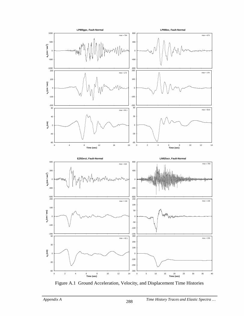
Appendix A Time History Traces and Elastic Spectra … 288
LP89lgpc, Fault-Normal
-1000
-500
0
500
1000
a g (c
m /
sec2 )
max = 704
LP89lex, Fault-Normal
-800
-400
0
400
800max = 673
-200
-100
0
100
200
v g (c
m /
sec)
max = 173
-200
-100
0
100
200max = 179
-80
-40
0
40
80
0 4 8 12 16 20Time (sec)
u g (c
m)
max = 65.1
-60
-30
0
30
60
0 2 4 6 8 10 12 14Time (sec)
max = 56.6
EZ92erzi, Fault-Normal
-600
-300
0
300
600
a g (c
m /
sec2 )
max = 424
LN92lucr, Fault-Normal
-800
-400
0
400
800max = 700
-200
-100
0
100
200
v g (c
m /
sec)
max = 119
-150
-100
-50
0
50
100
150max = 136
-60
-30
0
30
60
0 2 4 6 8 10 12 14Time (sec)
u g (c
m)
max = 42.1
-300
-200
-100
0
100
200
300
0 5 10 15 20 25 30 35 40Time (sec)
max = 230
Figure A.1 Ground Acceleration, Velocity, and Displacement Time Histories
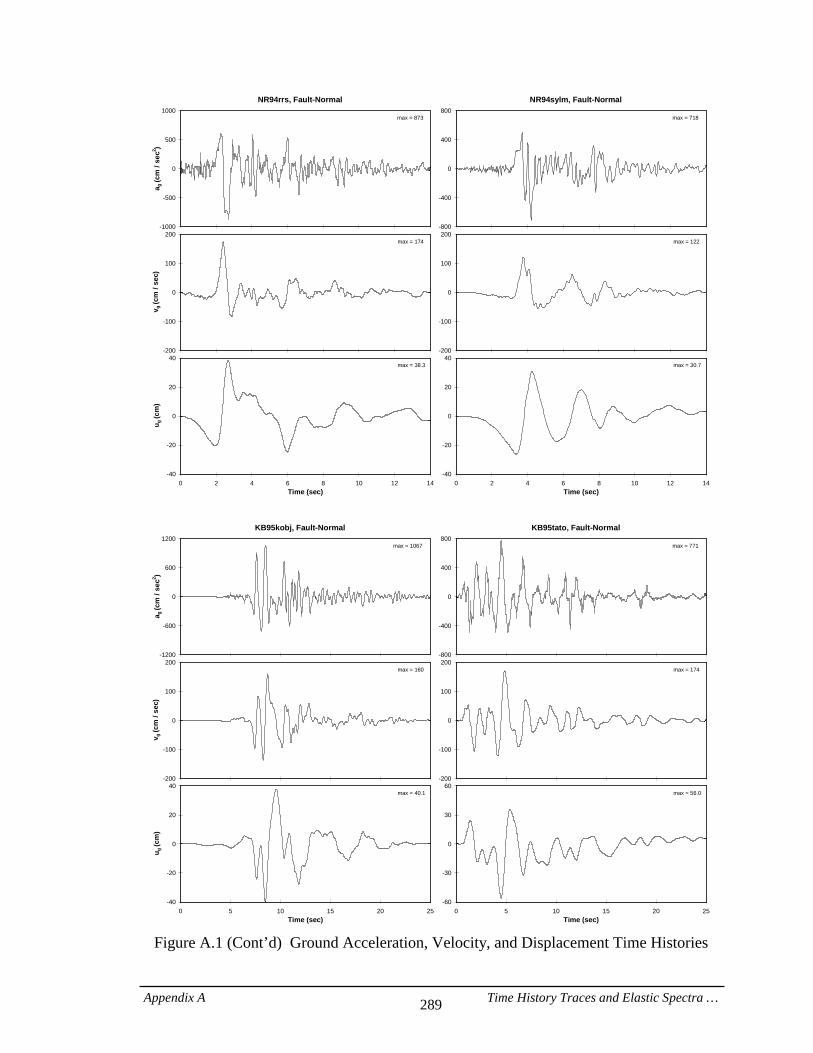
Appendix A Time History Traces and Elastic Spectra … 289
NR94rrs, Fault-Normal
-1000
-500
0
500
1000
a g (c
m /
sec2 )
max = 873
NR94sylm, Fault-Normal
-800
-400
0
400
800max = 718
-200
-100
0
100
200
v g (c
m /
sec)
max = 174
-200
-100
0
100
200max = 122
-40
-20
0
20
40
0 2 4 6 8 10 12 14Time (sec)
u g (c
m)
max = 38.3
-40
-20
0
20
40
0 2 4 6 8 10 12 14Time (sec)
max = 30.7
KB95kobj, Fault-Normal
-1200
-600
0
600
1200
a g (c
m /
sec2 )
max = 1067
KB95tato, Fault-Normal
-800
-400
0
400
800max = 771
-200
-100
0
100
200
v g (c
m /
sec)
max = 160
-200
-100
0
100
200max = 174
-40
-20
0
20
40
0 5 10 15 20 25Time (sec)
u g (c
m)
max = 40.1
-60
-30
0
30
60
0 5 10 15 20 25Time (sec)
max = 56.0
Figure A.1 (Cont’d) Ground Acceleration, Velocity, and Displacement Time Histories
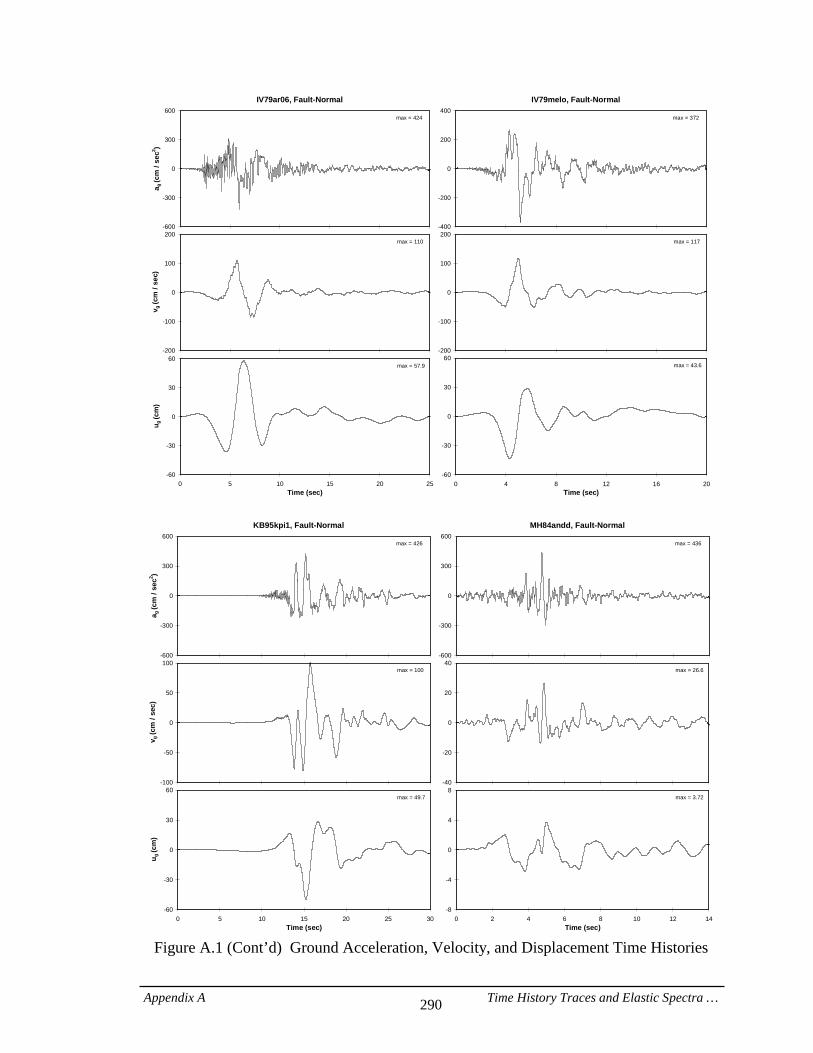
Appendix A Time History Traces and Elastic Spectra … 290
IV79ar06, Fault-Normal
-600
-300
0
300
600
a g (c
m /
sec2 )
max = 424
IV79melo, Fault-Normal
-400
-200
0
200
400max = 372
-200
-100
0
100
200
v g (c
m /
sec)
max = 110
-200
-100
0
100
200max = 117
-60
-30
0
30
60
0 5 10 15 20 25Time (sec)
u g (c
m)
max = 57.9
-60
-30
0
30
60
0 4 8 12 16 20Time (sec)
max = 43.6
KB95kpi1, Fault-Normal
-600
-300
0
300
600
a g (c
m /
sec2 )
max = 426
MH84andd, Fault-Normal
-600
-300
0
300
600max = 436
-100
-50
0
50
100
v g (c
m /
sec)
max = 100
-40
-20
0
20
40max = 26.6
-60
-30
0
30
60
0 5 10 15 20 25 30Time (sec)
u g (c
m)
max = 49.7
-8
-4
0
4
8
0 2 4 6 8 10 12 14Time (sec)
max = 3.72
Figure A.1 (Cont’d) Ground Acceleration, Velocity, and Displacement Time Histories
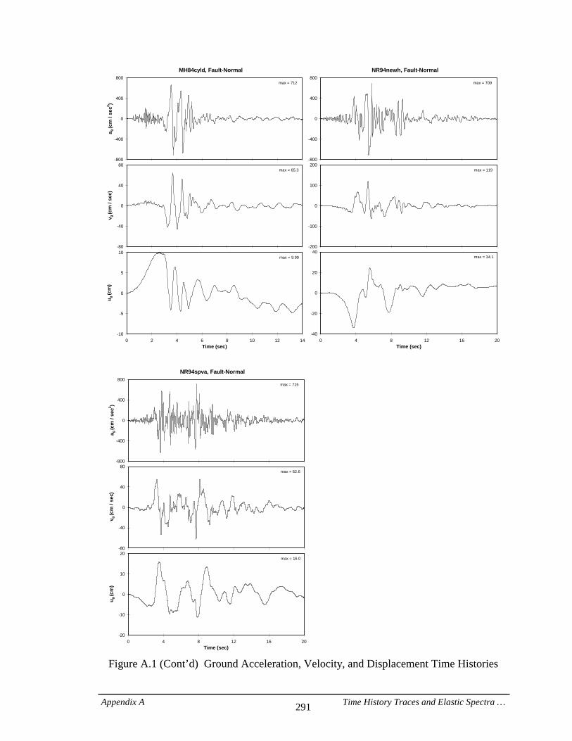
Appendix A Time History Traces and Elastic Spectra … 291
MH84cyld, Fault-Normal
-800
-400
0
400
800
a g (c
m /
sec2 )
max = 712
NR94newh, Fault-Normal
-800
-400
0
400
800max = 709
-80
-40
0
40
80
v g (c
m /
sec)
max = 65.3
-200
-100
0
100
200max = 119
-10
-5
0
5
10
0 2 4 6 8 10 12 14Time (sec)
u g (c
m)
max = 9.99
-40
-20
0
20
40
0 4 8 12 16 20Time (sec)
max = 34.1
NR94spva, Fault-Normal
-800
-400
0
400
800
a g (c
m /
sec2 )
max = 715
-80
-40
0
40
80
v g (c
m /
sec)
max = 62.6
-20
-10
0
10
20
0 4 8 12 16 20Time (sec)
u g (c
m)
max = 16.0
Figure A.1 (Cont’d) Ground Acceleration, Velocity, and Displacement Time Histories
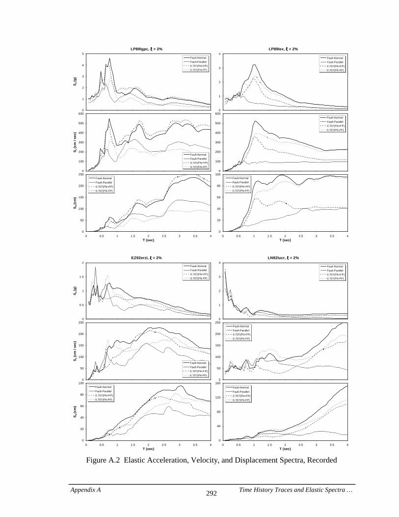
Appendix A Time History Traces and Elastic Spectra … 292
LP89lgpc, ξξξξ = 2%
0
1
2
3
4
5
S a (g
)
Fault-NormalFault-Parallel0.707(FN+FP)0.707(FN-FP)
LP89lex, ξξξξ = 2%
0
1
2
3
4Fault-NormalFault-Parallel0.707(FN+FP)0.707(FN-FP)
0
100
200
300
400
500
600
S v (c
m /
sec)
Fault-NormalFault-Parallel0.707(FN+FP)0.707(FN-FP)
0
100
200
300
400
500
600Fault-NormalFault-Parallel0.707(FN+FP)0.707(FN-FP)
0
50
100
150
200
250
0 0.5 1 1.5 2 2.5 3 3.5 4T (sec)
S d (c
m)
Fault-NormalFault-Parallel0.707(FN+FP)0.707(FN-FP)
0
20
40
60
80
100
0 0.5 1 1.5 2 2.5 3 3.5 4T (sec)
Fault-NormalFault-Parallel0.707(FN+FP)0.707(FN-FP)
EZ92erzi, ξξξξ = 2%
0
0.5
1
1.5
2
S a (g
)
Fault-NormalFault-Parallel0.707(FN+FP)0.707(FN-FP)
LN92lucr, ξξξξ = 2%
0
1
2
3
4Fault-NormalFault-Parallel0.707(FN+FP)0.707(FN-FP)
0
50
100
150
200
250
S v (c
m /
sec)
Fault-NormalFault-Parallel0.707(FN+FP)0.707(FN-FP)
0
50
100
150
200
250Fault-NormalFault-Parallel0.707(FN+FP)0.707(FN-FP)
0
20
40
60
80
100
0 0.5 1 1.5 2 2.5 3 3.5 4T (sec)
S d (c
m)
Fault-NormalFault-Parallel0.707(FN+FP)0.707(FN-FP)
0
40
80
120
160
0 0.5 1 1.5 2 2.5 3 3.5 4T (sec)
Fault-NormalFault-Parallel0.707(FN+FP)0.707(FN-FP)
Figure A.2 Elastic Acceleration, Velocity, and Displacement Spectra, Recorded
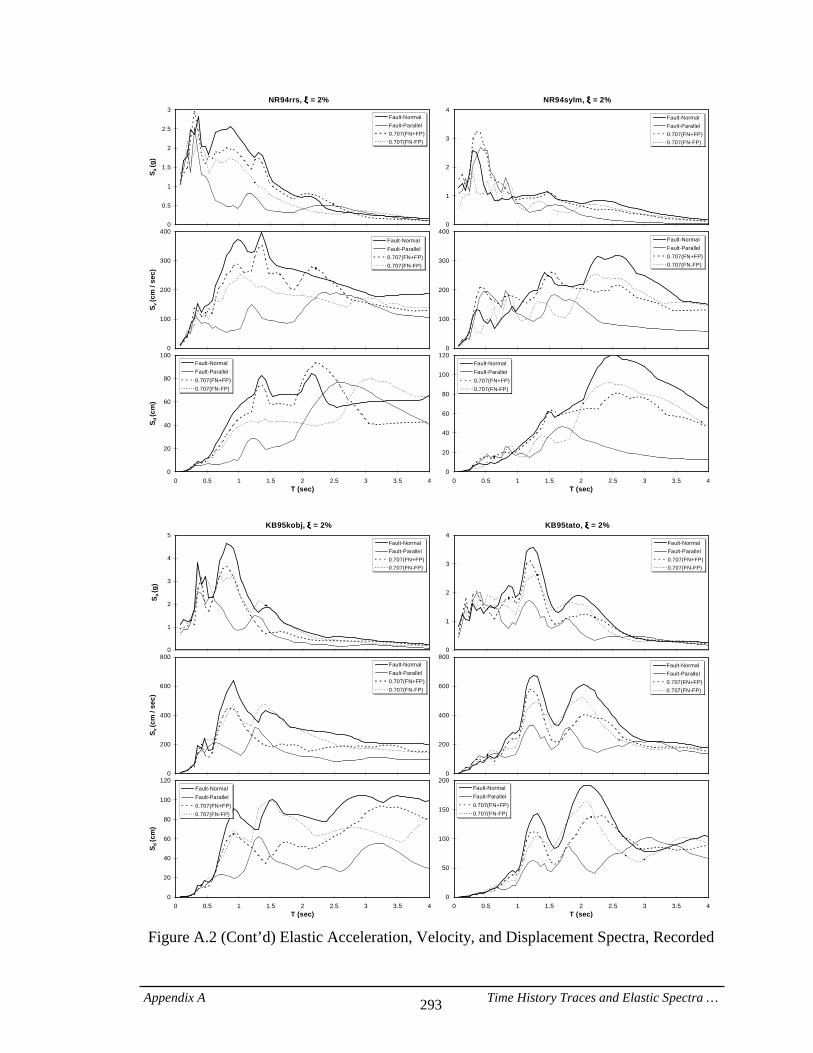
Appendix A Time History Traces and Elastic Spectra … 293
NR94rrs, ξξξξ = 2%
0
0.5
1
1.5
2
2.5
3
S a (g
)
Fault-NormalFault-Parallel0.707(FN+FP)0.707(FN-FP)
NR94sylm, ξξξξ = 2%
0
1
2
3
4Fault-NormalFault-Parallel0.707(FN+FP)0.707(FN-FP)
0
100
200
300
400
S v (c
m /
sec)
Fault-NormalFault-Parallel0.707(FN+FP)0.707(FN-FP)
0
100
200
300
400Fault-NormalFault-Parallel0.707(FN+FP)0.707(FN-FP)
0
20
40
60
80
100
0 0.5 1 1.5 2 2.5 3 3.5 4T (sec)
S d (c
m)
Fault-NormalFault-Parallel0.707(FN+FP)0.707(FN-FP)
0
20
40
60
80
100
120
0 0.5 1 1.5 2 2.5 3 3.5 4T (sec)
Fault-NormalFault-Parallel0.707(FN+FP)0.707(FN-FP)
KB95kobj, ξξξξ = 2%
0
1
2
3
4
5
S a (g
)
Fault-NormalFault-Parallel0.707(FN+FP)0.707(FN-FP)
KB95tato, ξξξξ = 2%
0
1
2
3
4Fault-NormalFault-Parallel0.707(FN+FP)0.707(FN-FP)
0
200
400
600
800
S v (c
m /
sec)
Fault-NormalFault-Parallel0.707(FN+FP)0.707(FN-FP)
0
200
400
600
800Fault-NormalFault-Parallel0.707(FN+FP)0.707(FN-FP)
0
20
40
60
80
100
120
0 0.5 1 1.5 2 2.5 3 3.5 4T (sec)
S d (c
m)
Fault-NormalFault-Parallel0.707(FN+FP)0.707(FN-FP)
0
50
100
150
200
0 0.5 1 1.5 2 2.5 3 3.5 4T (sec)
Fault-NormalFault-Parallel0.707(FN+FP)0.707(FN-FP)
Figure A.2 (Cont’d) Elastic Acceleration, Velocity, and Displacement Spectra, Recorded
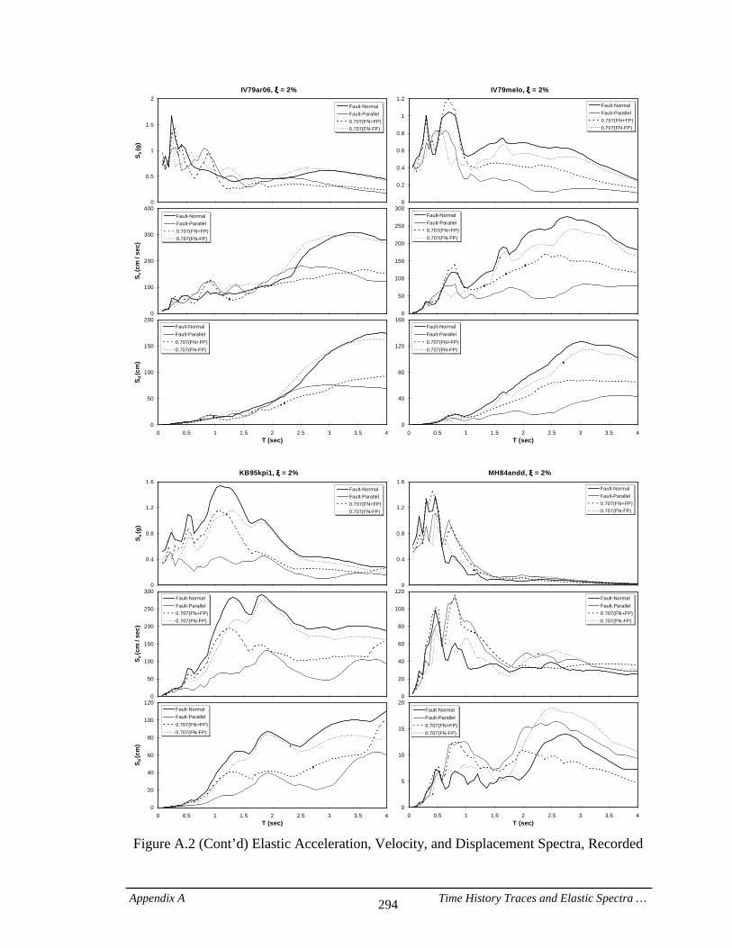
Appendix A Time History Traces and Elastic Spectra … 294
IV79ar06, ξξξξ = 2%
0
0.5
1
1.5
2
S a (g
)
Fault-NormalFault-Parallel0.707(FN+FP)0.707(FN-FP)
IV79melo, ξξξξ = 2%
0
0.2
0.4
0.6
0.8
1
1.2Fault-NormalFault-Parallel0.707(FN+FP)0.707(FN-FP)
0
100
200
300
400
S v (c
m /
sec)
Fault-NormalFault-Parallel0.707(FN+FP)0.707(FN-FP)
0
50
100
150
200
250
300Fault-NormalFault-Parallel0.707(FN+FP)0.707(FN-FP)
0
50
100
150
200
0 0.5 1 1.5 2 2.5 3 3.5 4T (sec)
S d (c
m)
Fault-NormalFault-Parallel0.707(FN+FP)0.707(FN-FP)
0
40
80
120
160
0 0.5 1 1.5 2 2.5 3 3.5 4T (sec)
Fault-NormalFault-Parallel0.707(FN+FP)0.707(FN-FP)
KB95kpi1, ξξξξ = 2%
0
0.4
0.8
1.2
1.6
S a (g
)
Fault-NormalFault-Parallel0.707(FN+FP)0.707(FN-FP)
MH84andd, ξξξξ = 2%
0
0.4
0.8
1.2
1.6Fault-NormalFault-Parallel0.707(FN+FP)0.707(FN-FP)
0
50
100
150
200
250
300
S v (c
m /
sec)
Fault-NormalFault-Parallel0.707(FN+FP)0.707(FN-FP)
0
20
40
60
80
100
120Fault-NormalFault-Parallel0.707(FN+FP)0.707(FN-FP)
0
20
40
60
80
100
120
0 0.5 1 1.5 2 2.5 3 3.5 4T (sec)
S d (c
m)
Fault-NormalFault-Parallel0.707(FN+FP)0.707(FN-FP)
0
5
10
15
20
0 0.5 1 1.5 2 2.5 3 3.5 4T (sec)
d
Fault-NormalFault-Parallel0.707(FN+FP)0.707(FN-FP)
Figure A.2 (Cont’d) Elastic Acceleration, Velocity, and Displacement Spectra, Recorded
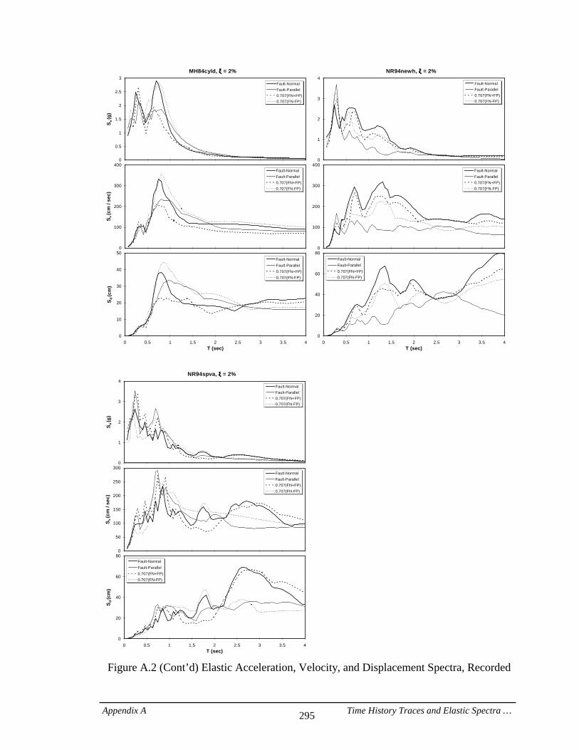
Appendix A Time History Traces and Elastic Spectra … 295
MH84cyld, ξξξξ = 2%
0
0.5
1
1.5
2
2.5
3
S a (g
)
Fault-NormalFault-Parallel0.707(FN+FP)0.707(FN-FP)
NR94newh, ξξξξ = 2%
0
1
2
3
4Fault-NormalFault-Parallel0.707(FN+FP)0.707(FN-FP)
0
100
200
300
400
S v (c
m /
sec)
Fault-NormalFault-Parallel0.707(FN+FP)0.707(FN-FP)
0
100
200
300
400Fault-NormalFault-Parallel0.707(FN+FP)0.707(FN-FP)
0
10
20
30
40
50
0 0.5 1 1.5 2 2.5 3 3.5 4T (sec)
S d (c
m)
Fault-NormalFault-Parallel0.707(FN+FP)0.707(FN-FP)
0
20
40
60
80
0 0.5 1 1.5 2 2.5 3 3.5 4T (sec)
Fault-NormalFault-Parallel0.707(FN+FP)0.707(FN-FP)
NR94spva, ξξξξ = 2%
0
1
2
3
4
S a (g
)
Fault-NormalFault-Parallel0.707(FN+FP)0.707(FN-FP)
0
50
100
150
200
250
300
S v (c
m /
sec)
Fault-NormalFault-Parallel0.707(FN+FP)0.707(FN-FP)
0
20
40
60
80
0 0.5 1 1.5 2 2.5 3 3.5 4T (sec)
S d (c
m)
Fault-NormalFault-Parallel0.707(FN+FP)0.707(FN-FP)
Figure A.2 (Cont’d) Elastic Acceleration, Velocity, and Displacement Spectra, Recorded
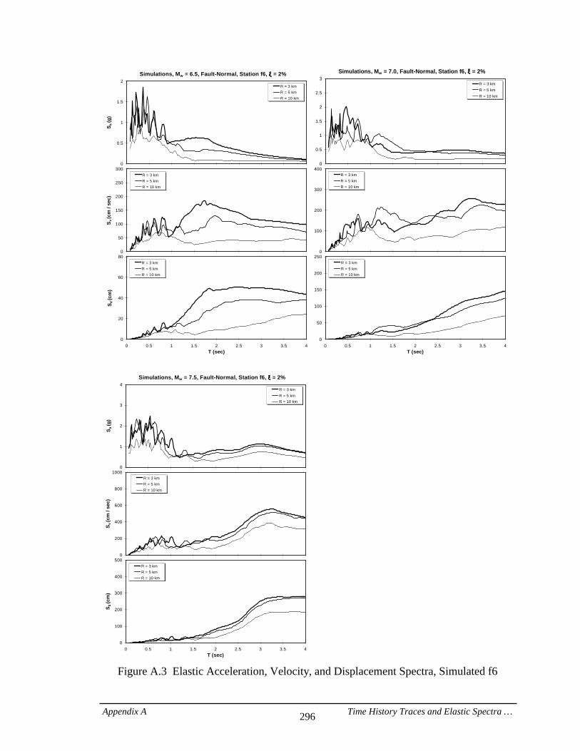
Appendix A Time History Traces and Elastic Spectra … 296
Simulations, Mw = 6.5, Fault-Normal, Station f6, ξξξξ = 2%
0
0.5
1
1.5
2
S a (g
)
R = 3 kmR = 5 kmR = 10 km
Simulations, Mw = 7.0, Fault-Normal, Station f6, ξξξξ = 2%
0
0.5
1
1.5
2
2.5
3R = 3 kmR = 5 kmR = 10 km
0
50
100
150
200
250
300
S v (c
m /
sec)
R = 3 kmR = 5 kmR = 10 km
0
100
200
300
400R = 3 kmR = 5 kmR = 10 km
0
20
40
60
80
0 0.5 1 1.5 2 2.5 3 3.5 4T (sec)
S d (c
m)
R = 3 kmR = 5 kmR = 10 km
0
50
100
150
200
250
0 0.5 1 1.5 2 2.5 3 3.5 4T (sec)
R = 3 kmR = 5 kmR = 10 km
Simulations, Mw = 7.5, Fault-Normal, Station f6, ξξξξ = 2%
0
1
2
3
4
S a (g
)
R = 3 kmR = 5 kmR = 10 km
0
200
400
600
800
1000
S v (c
m /
sec)
R = 3 kmR = 5 kmR = 10 km
0
100
200
300
400
500
0 0.5 1 1.5 2 2.5 3 3.5 4T (sec)
S d (c
m)
R = 3 kmR = 5 kmR = 10 km
Figure A.3 Elastic Acceleration, Velocity, and Displacement Spectra, Simulated f6
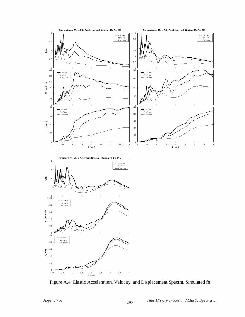
Appendix A Time History Traces and Elastic Spectra … 297
Simulations, Mw = 6.5, Fault-Normal, Station f8, ξξξξ = 2%
0
0.5
1
1.5
2
S a (g
)
R = 3 kmR = 5 kmR = 10 km
Simulations, Mw = 7.0, Fault-Normal, Station f8, ξξξξ = 2%
0
0.5
1
1.5
2
2.5
3R = 3 kmR = 5 kmR = 10 km
0
50
100
150
200
250
300
S v (c
m /
sec)
R = 3 kmR = 5 kmR = 10 km
0
100
200
300
400R = 3 kmR = 5 kmR = 10 km
0
20
40
60
80
0 0.5 1 1.5 2 2.5 3 3.5 4T (sec)
S d (c
m)
R = 3 kmR = 5 kmR = 10 km
0
50
100
150
200
250
0 0.5 1 1.5 2 2.5 3 3.5 4T (sec)
R = 3 kmR = 5 kmR = 10 km
Simulations, Mw = 7.5, Fault-Normal, Station f8, ξξξξ = 2%
0
1
2
3
4
S a (g
)
R = 3 kmR = 5 kmR = 10 km
0
200
400
600
800
1000
S v (c
m /
sec)
R = 3 kmR = 5 kmR = 10 km
0
100
200
300
400
500
0 0.5 1 1.5 2 2.5 3 3.5 4T (sec)
S d (c
m)
R = 3 kmR = 5 kmR = 10 km
Figure A.4 Elastic Acceleration, Velocity, and Displacement Spectra, Simulated f8
List of References 298
LIST OF REFERENCES
Abrahamson, N., and Silva, W., (1997). “Empirical Response Spectral Attenuation Relations for Shallow Crustal Earthquakes,” Seismological Research Letters, Vol. 68, No.1, 94-126. ACI 318-99 (1999). “Building Code Requirements for Structural Concrete and Commentary,” American Concrete Institute, Farmington Hills, Michigan, 1999. Anderson, J., and Bertero, V., (1978). “Uncertainties in Establishing Design Earthquakes,” ASCE Journal of Structural Engineering, Vol. 113, No. 8, Aug. 1987, 1709-1724. Anderson, J., Bertero, V., and Bertero, R., (1999). “Performance Improvement of Long Period Building Structures Subjected to Severe Pulse-Type Ground Motions,” Pacific Earthquake Engineering Research Center, University of California, Berkeley, Report No. PEER-1999/09, Oct. 1999. Baez, J., and Miranda, E., (2000). “Amplification Factors to Estimate Inelastic Displacement Demands for the Design of Structures in the Near Field,” Proceedings, 12th World Conference on Earthquake Engineering, New Zealand. Benioff, H., (1955). “Mechanism and Strain Characteristics of the White Wolf Fault as Indicated by the Aftershock Sequence, Earthquakes in Kern County, California, During 1955 (G.B. Oakeshotte, ed.),” California Division of Mines Bulletin, No. 171, 199-202.
List of References 299
Bertero, V., Mahin, S., and Herrera, R., (1978). “Aseismic Design Implications of Near-Fault San Fernando Earthquake Records,” Earthquake Engineering and Structural Dynamics, Vol. 6, Jan.-Feb. 1978, 31-42. Biggs, J., (1964). “Introduction to Structural Dynamics,” McGraw-Hill, Inc., New York. Chopra, A., (1995). “Dynamics of Structures: Theory and Applications to Earthquake Engineering,” Prentice-Hall, Inc., Englewood Cliffs, New Jersey, 131-151. Graves, R. (1996). “Modification of Lucerne Time History of the 1992 Landers Earthquake to Include Geodetically Defined Static Displacements,” Unpublished Manuscript. Gupta, A., and Krawinkler, H., (1999). “Seismic Demands for Performance Evaluation of Steel Moment Resisting Frame Structures,” John A. Blume Earthquake Engineering Center, Report No. 132, Department of Civil Engineering, Stanford University. Gupta, A., and Krawinkler, H., (2000). “Dynamic P-delta Effects for Flexible Inelastic Steel Structures,” ASCE Journal of Structural Engineering, Vol. 126, No. 1, Jan. 2000, 145-154. Hall, J., Heaton, T., Halling, M., Wald, D., (1995). “Near-Source Ground Motion and its Effects on Flexible Buildings,” Earthquake Spectra, Vol. 11, No. 4, Nov. 1995, 569-605. Iwan, W., and Chen, X., (1994). “Important Near-Field Ground Motion Data from the Landers Earthquake,” Proceedings, 10th European Conference on Earthquake Engineering, Vienna. Iwan, W., (1997). “Drift Spectrum: Measure of Demand for Earthquake Ground Motions,” ASCE Journal of Structural Engineering, Vol. 123, No. 4, Apr. 1997, 397-404. Krawinkler, H., and Gupta, A., (1998). “Story Drift Demands for Steel Moment Frame Structures in Different Seismic Regions,” Proceedings, Sixth U.S. National Conference on Earthquake Engineering, Seattle, Washington. Lawson, R., (1996). “Site-Dependent Inelastic Seismic Demands,” Ph.D. Dissertation, Department of Civil Engineering, Stanford University. MacRae, G., Morrow, D., and Roeder, C., (1998). “Near-Field Ground Motion Effects on Short Structures,” PG&E-PEER Program, University of Washington, Draft Report, Aug. 1998. Mahin, S., Bertero, V., Chopra, A., and Collins, R., (1976). “Response of the Olive View Hospital Main Building During the San Fernando Earthquake,” Earthquake Engineering Research Center, University of California, Berkeley, Report No.UCB/EERC-76/22, Oct. 1976.
List of References 300
Makris, N., and Chang, S., (2000). “Effect of Viscous, Viscoplastic and Friction Damping on the Response of Seismic Isolated Structures,” Earthquake Engineering & Structural Dynamics, Vol. 29, No.1, Jan. 2000, 85-107. Nassar, A., and Krawinkler, H., (1991). “Seismic Demands for SDOF and MDOF systems,” John A. Blume Earthquake Engineering Center, Report No. 95, Department of Civil Engineering, Stanford University. NEHRP (1994). “National Earthquake Hazards Reduction Program Recommended Provisions for Seismic Regulations for New Buildings,” Federal Emergency Management Agency 223, Washington, DC, 1994. Prakash, V., Powell, G.H., and Campbell, S., (1993). “DRAIN-2DX Base Program Description and User Guide, Version 1.10”, Report No. UCB/SEMM-93/17, Department of Civil Engineering, University of California at Berkeley. Rahnama, M., and Krawinkler, H., (1993). “Effects of Soft Soils and Hysteresis Model on Seismic Demands,” John A. Blume Earthquake Engineering Center, Report No. 108, Department of Civil Engineering, Stanford University. Ramsey, F., and Schafer, D., (1996). “The Statistical Sleuth: A Course in Methods of Data Analysis,” Duxbury Press, Belmont, California,181-186. SEAOC Blue Book (1996). “Recommended Lateral Force Requirements and Commentary,” Structural Engineers Association of California, sixth edition, Sacramento, California, 1996. Seneviratna, G.D.P.K., and Krawinkler, H., (1997). “Evaluation of Inelastic MDOF Effects for Seismic Design,” John A. Blume Earthquake Engineering Center, Report No. 120, Department of Civil Engineering, Stanford University. Silva, W., (1999). “Strong Motion Database,” CD-ROM, Pacific Engineering and Analysis (also available at http://peer.berkeley.edu/smcat). Singh, J., (1985). “Earthquake Ground Motions: Implications for Designing Structures and Reconciling Structural Damage,” Earthquake Spectra, Feb. 1985, 239-270. Somerville, P., Saikia C.K., Wald, D., and Graves, R. (1996). “Implications of the Northridge Earthquake for Strong Ground Motions from Thrust Faults,” Bulletin of the Seismological Society of America, 86, S115-S125. Somerville, P., Smith N., Punyamurthula, S., and Sun, J. (1997a). “Development of Ground Motion Time Histories for Phase 2 of the FEMA/SAC Steel Project,” Report No. SAC/BD-97-04.
List of References 301
Somerville, P., Smith, N., Graves, R., and Abrahamson, N., (1997b). “Modification of Empirical Strong Ground Motion Attenuation Relations to Include the Amplitude and Duration Effects of Rupture Directivity,” Seismological Research Letters, Vol. 68, No. 1, 180-203. Somerville, P., (1998). “Development of an Improved Ground Motion Representation for Near Fault Ground Motions,” SMIP98 Seminar on Utilization of Strong-Motion Data, Oakland, CA, Sept. 1998. Somerville, P., (2000). “Characterization of Near Fault Ground Motions,” US-Japan Workshop on Effects of Near-Field Earthquake Shaking, San Francisco, CA, March 2000. Uniform Building Code (1997). International Conference of Building Officials, Whittier, California. Veletsos, A. and Newmark, N., and Chelapati, C., (1965). “Deformation Spectra for Elastic and Elastoplastic Systems Subjected to Ground Shock and Earthquake Motions,” Proceeding, Third World Conference on Earthquake Engineering, Vol. II, New Zealand. Wald, D., and Heaton, T., (1994). “Spatial and Temporal Distribution of Slip for the 1992 Landers, California, Earthquake,” Bulletin of the Seismological Society of America, 84, 668-691.