Research Article The Seismic Response of High-Speed...

Research ArticleThe Seismic Response of High-Speed Railway BridgesSubjected to Near-Fault Forward Directivity Ground MotionsUsing a Vehicle-Track-Bridge Element

Chen Ling-kun,1,2 Jiang Li-zhong,2,3 Guo Wei,2,3 Liu Wen-shuo,2,3

Zeng Zhi-ping,2,3 and Chen Ge-wei4

1 College of Civil Science and Engineering, Yangzhou University, Yangzhou 225127, China2National Engineering Laboratory for High-Speed Railway Construction, Central South University, Changsha 410075, China3 School of Civil Engineering, Central South University, Changsha 410075, China4Department of Civil and Engineering, University of Auckland, Auckland 1142, New Zealand

Correspondence should be addressed to Chen Ling-kun; [email protected]

Received 15 July 2013; Accepted 1 November 2013; Published 27 February 2014

Academic Editor: Vadim V. Silberschmidt

Copyright © 2014 Chen Ling-kun et al.This is an open access article distributed under the Creative Commons Attribution License,which permits unrestricted use, distribution, and reproduction in any medium, provided the original work is properly cited.

Based on theNextGenerationAttenuation (NGA) project groundmotion library, the finite elementmodel of the high-speed railwayvehicle-bridge system is established. The model was specifically developed for such system that is subjected to near-fault groundmotions. In addition, it accounted for the influence of the rail irregularities.The vehicle-track-bridge (VTB) element is presented tosimulate the interaction between train and bridge, in which a train can be modeled as a series of sprung masses concentrated at theaxle positions. For the short period railway bridge, the results from the case study demonstrate that directivity pulse effect tends toincrease the seismic responses of the bridge compared with far-fault ground motions or nonpulse-like motions and the directivitypulse effect and high values of the vertical acceleration component can notably influence the hysteretic behaviour of piers.

1. Introduction

In principle, when an earthquake fault ruptures and propa-gates towards a site at a speed close to the shear wave velocity,the generated waves will arrive at the site at approximatelythe same time. This creates the cumulative effect of almostall of the seismic energy radiation from fault and generatesa “distinct” velocity pulse within the ground motion timehistory, at a strike-normal direction [1].

Figure 1 portrays the three zones of directivity. Thecircle representing the epicenter and the black line indicatesthe fault. According to the model, site B (Figure 2) wouldexperience a longer interval of the time interval between thearrivals of the waves; thus, the record at site B would have along duration but not a velocity pulse. Intense velocity pulseusually occurs at the beginning of a record. Its occurrenceis referred to as the FD effect. For more than a decade, theFD effect has been known to have potential to cause severe

damage in a structure and in turn cause relatively severeelastic and inelastic responses in structures during certainperiods. Figure 3 illustrates ground acceleration, velocity,and displacement time-history traces for the fault-normalcomponent of a typical near-fault ground motion with FD(Northridge 1994 Rinaldi Receiving Station). As indicatedparticularly by the velocity and displacement traces, therecord contains a large pulse within the time range fromabout 2 to 3 sec. To further comparison, a nonpulse recordfrom the Northridge 1994, Century City CC North is alsoshown.

Rupture directivity has been long recognized sinceBenioff [2] and Kasahara [3]. In the recordings of largeearthquakes and further, it has been theoretically explainedby early kinematic models of line sources by Haskell [4],Ben-Menahem [5] who introduced the rupture directivitycoefficient of 𝐶𝑑. This effect has been observed on strongground motion records in the near-fault region, for instance,

Hindawi Publishing CorporationShock and VibrationVolume 2014, Article ID 985602, 17 pageshttp://dx.doi.org/10.1155/2014/985602

2 Shock and Vibration

Seismogenicdepth

Epicenter

Reverse

Forward

Neutral

Figure 1: Zone of directivity.

Epicenter

Site A

Site B

Figure 2: An example of FD effect on Site A.

as the 𝑀𝑊 6.6 1971 San Fernando earthquake [6], the 𝑀𝑊

6.6 1979 Emperial valley earthquake [7], the 𝑀𝑊 6.7 1994Northridge earthquake [8], the 𝑀𝑊 7.2 1995 Hyogoken-Nanbu (Kobe) earthquake [9], the 𝑀𝑊 7.6 1999 Chi-Chi,Taiwan earthquake [10], and𝑀𝑊 7.4 1999 Kocaeli earthquake[11].

Ground motions with a pulse at the beginning of thevelocity time history belong to a special class of groundmotion that causes severe damage in structures. This classof ground motions, which are indicated by the presence ofa velocity pulse, can cause large responses in structures. Theinfluence of near-fault pulse-like ground motions on theseismic response of structure has become a very importanttopic to lots of researchers in recently years. Alavi andKrawinkler [12] studied the response spectrum pulse aswould earthquakes with the FD effect be studied. It wasstated that the velocity effect could greatly influence thenonlinear response of the structure. Choi et al. [13] investigatethe near-fault ground motion effects on typical Caltransbridge columns to develop practical and proven bridge designguidelines that incorporate the effects of near-fault groundmotions. Mortezaei and Ronagh [14] performed the inelastictime-history analyses to predict the nonlinear behaviour

of RC columns that were subjected to both far-fault andnear-fault earthquakes, both of which contain a FD effect.MacRae et al. [15] studied the effects of earthquake groundmotions on the response of SDOF oscillators with elastic-perfectly plastic hysteresis behavior. Tothong and Cornell[16] demonstrated the effectiveness of utilizing advancedground motion intensity measures to evaluate the seismicperformance of a structure subject to near-source groundmotions. Baker and Cornell [17] considered a vector-valuedintensity measure (IM) to account for the effects of pulse-like near-fault ground motions. Xu et al. [18] investigatedthe application of equivalent pulses to the parameter atten-uation relationships developed for near-fault FD motions.Chioccarelli and Iervolino [19] investigated the velocity pulseeffect of horizontal components of L’Aquila earthquake.Theirresearch indicated that the vertical components of motiondid not provide clear evidence of directivity effects in therupture-normal direction. Mazza and Vulcano [20] studiedthe nonlinear dynamic response of an r. c. framed buildingslocated in a near-fault area, in reference to the horizontal andvertical components of near-fault records. Chen et al. [21–24] carried out a series of research on the seismic responseof the high-speed railway bridge, discovering some useful

Shock and Vibration 3

0.0

0.2

0.4

0.6

0.8

1.0

1.2

Acce

lera

tion

(g)

−1.0

−0.8

−0.6

−0.4

−0.2

0 2 4 6 8 10 12 14Time (s)

0.838

(a) Acceleration time-history curve

0

50

100

150

200

Velo

city

(cm

/s)

−50

−1000 2 4 6 8 10 12 14

Time (s)

166.05

TP

(b) Velocity time-history curve

0

10

20

30

−30

−20

−10

0 2 4 6 8 10 12 14Time (s)

Disp

lace

men

t (cm

)

Northridge-Rinaadi Northridge-Century City CC North

28.78

(c) Displacement time-history curve

Figure 3: Ground acceleration, velocity, and displacement time histories for record of Northridge Rinaldi and Century City CC North.

conclusions that would assist the seismic design of the railwaybridge.

The existing research on the near-fault earthquakefocuses mainly on the basic properties and the focal mecha-nisms. Some research on the seismic dynamic response of thebridge was carried out recently. It concentrated on buildingstructures and highway bridges [25–28], as recommendedin recent regulatory design codes and provisions such asATC-40 (1996) and IBC (ICBO 2000). The site-source anddistance-dependent near-source factors 𝑁𝐴 and 𝑁𝑉 whichconsider FD effect were then introduced to amplify theelastic design spectrum and scale the design base shear.There is minimal research on the seismic response of therailway bridge, characterized by the unneglected movingtrain loading and the ballastless structure above the boxinggirder bridge, and most existing railway bridge structureswere designed without considering any “near-fault” feature[29, 30].

In this paper, a train can be modeled as a series ofsprung masses concentrated at the axle positions using theVTB element. The finite element model of the multispansimply supported high-speed railway bridge is set up basedon the PEER NAG Strong Ground Motion Database. Theseismic performance of short-period high-speed railwaybridge under rupture FD pulse-like ground motions wasinvestigated. Furthermore, the rupture FD and high verticalground motions effects were considered.

2. Model of Vehicle-Bridge System

The train loading is one of the dominant factors in the designand the dynamic analysis of the railway bridges. Apart fromthe simplified design live load pattern of railway bridges inpassenger-specific lines, as well as in passenger and freightmixed lines (which were adopted in the general designspecifications [31], on the dynamics of bridges under moving


trains), there are three main types of train models to be used:(1) the moving force model, (2) the moving mass model,and (3) the moving multi-rigid-body system model. Zhangand Xia [32], Gao and Pan [33], Li et al. [34], and Jo et al.[35]modeled the vehicle and the bridge subsystem separately.Yang and Wu [36] investigate the vibration of simple beamssubjected to the passage of high-speed trains, where the trainismodeled as a series of sprungmasses. By using themodifiedbeam vibration functions as the assumed modes, Cheunget al. [37] analyzed the vibration of multispan nonuniformbridges under a moving train. Although the model cannotrealistically predict the response of the vehicle, the model canobtain the closed-form solutions for some problems.

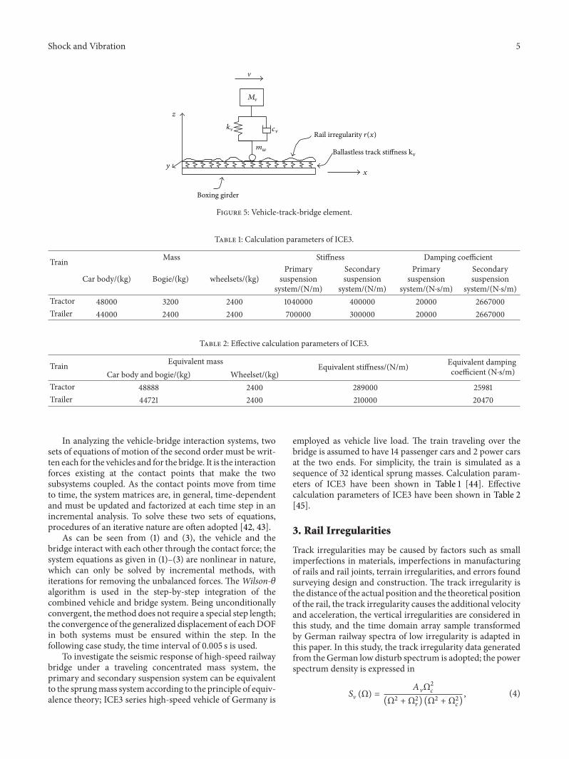
In this study, a global bridgemodel is developed as shownin Figure 4. The train is traveling over the bridge with aconstant speed V. It is idealized as a series of lumped massessupported by the suspension systems, as represented by thesprings and dashpots, which in turn are acting on the bridge.A train bridge interaction element is presented in when theCRTS II layered slab ballastless track (i.e., China RailwayTrack System II Type Ballastless Slab Tracks) is introduced tothemodel based on the existing research [36, 37]. It consists ofa bridge (boxing girder) element and suspension units of thecar bodies directly acting on it, as shown in Figure 5, wherethe rail irregularity 𝑟(𝑥) and CRTS II layered slab ballastlesstrack stiffness 𝑘𝐵 are also indicated. In thismodel, the columnbases are assumed to be rigidly connected to the pile caps,which are in turn assumed to be fully fixed; hence no soil orpile deformation effects are included.

As the model of the VTB element is depicted in Figure 5,a train can be modeled as a series of sprung masses concen-trated at the axle positions, of which the suspension device isrepresented by a spring-dashpot system model, and a bridgeas a series of 3D beam elements. In this study, the notation[ ] is used for a square matrix or a row vector, and { } isused for a column vector. The following notation is adopted:𝑟(𝑥) = rail irregularity, 𝑘𝐵 = ballastless track stiffness, 𝑘V =suspension stiffness, 𝑐V = suspension damping, 𝑚𝑤 = wheelmass, and𝑀V = lumped vehiclemass. In addition, the verticaldeflections of the wheel and car body masses from the staticequilibrium position are denoted as {𝑧}𝑇 = [𝑧𝑊, 𝑧𝑀] by thegeneralized coordinates, 𝑧𝑤 = the vertical displacements ofthe wheel-sets, and 𝑧𝑀 = the vertical displacements of thesprung masses, corresponding to the nodal displacements{𝑧}𝑇, the external forces, {𝑝}𝑇 = [𝑝V, 𝑝𝑔], where 𝑝V = −(𝑀V +

𝑚𝑤)𝑔, 𝑔 = the acceleration of gravity, and 𝑓V𝑔 = earthquakeloading of the train.

The equations ofmotion for the vehiclemasses in Figure 5can be written, based on Jo et al. [35] and Xia et al. [38]equations:

[𝑚𝑤 0

0 𝑀V]{

��𝑤

��𝑀} + [

𝑐V −𝑐V−𝑐V 𝑐V

]{��𝑤

��𝑀} + [

𝑘V −𝑘V−𝑘V 𝑘V

]{𝑧𝑤

𝑧𝑀}

= {𝑝V + 𝑓𝑐

−𝑓V𝑔} ,

(1)

�VTB element

(a) Schematic diagram

y (lateral)

x (longitudinal)

z (vertical)

(b) Coordinate law

Figure 4: Global model of vehicle-bridge systems.

where 𝑓𝑐 denotes the interaction force existing betweenthe as wheel-sets and the bridge element. By letting 𝑥𝑐

denote the position of the contact point and {𝑁𝑐} a vectorobtaining the shape functions of the vertical displacementinvolving the beam evaluated at the contact point 𝑥𝑐, that is,Hermitian interpolation functions, that is, {𝑁𝑐} = {𝑁𝑖(𝑥𝑐)},the interaction force can be expressed as

𝑓𝑐 = 𝑘𝐵 ({𝑁𝑐} [𝑢𝑏] + 𝑟𝑐 − 𝑧𝑤) , (2)

where the condition of 𝑓𝑐 ≥ 0 is imposed to exclude theseparation of the vehicle from the bridge. In other terms, it 𝑡is assumed that the wheel-track interaction obeys the wheel-track corresponding assumption in the vertical direction;𝑘𝐵 = ballast stiffness; the value of 20MN/m per rail has beenused byNielsen andAbrahamsson [39], Yau et al. [40] is takenas 40MN/m for two rails. CRTS II layered slab ballastlesstrack is used in this study; according to the wheel drop loadtest [41], 𝑘𝐵 = 105 kN/mm; [𝑢𝑏] = the nodal displacements ofthe beam; and 𝑟𝑐 = the rail irregularity at the contact point𝑥𝑐.

The deck of bridge and the piers are idealized as a linearelastic Bernoulli-Euler beam, containing a uniform section.The bridge piers are assumed to remain in the elastic stateduring the earthquake excitation, which are also assumedto be rigidly fixed at the foundation level. The bridge pierelements can be assembled by conventional procedures, toform the equations of motion for the entire bridge structure.The equations ofmotion for the bridge element can bewrittenas

[𝑚𝑏] {��𝑏} + [𝑐𝑏] {��𝑏} + [𝑘𝑏] {𝑢𝑏} = 𝑝𝑏 − {𝑁𝑐} 𝑓𝑐 + 𝑓𝑏𝑔, (3)

where [𝑚𝑏], [𝑐𝑏], and [𝑘𝑏] = the mass, damping, and stiffnessmatrices of the bridge element, 𝑝𝑏 = the external nodalloads, and 𝑓𝑏𝑔 = the earthquake loading of the bridge. Thetwo factors of Rayleigh damping 𝑐(Damping) = 𝛼(Mass) +𝛽(Stiffness). 𝛼 and 𝛽 can be given by eigenvalue analysis.


�

z

yx

mw

Rail irregularity r(x)

Ballastless track stiffness kv

Boxing girder

Mv

cvkv

Figure 5: Vehicle-track-bridge element.

Table 1: Calculation parameters of ICE3.

Train Mass Stiffness Damping coefficient

Car body/(kg) Bogie/(kg) wheelsets/(kg)Primary

suspensionsystem/(N/m)

Secondarysuspension

system/(N/m)

Primarysuspension

system/(N⋅s/m)

Secondarysuspension

system/(N⋅s/m)Tractor 48000 3200 2400 1040000 400000 20000 2667000Trailer 44000 2400 2400 700000 300000 20000 2667000

Table 2: Effective calculation parameters of ICE3.

Train Equivalent mass Equivalent stiffness/(N/m) Equivalent dampingcoefficient (N⋅s/m)Car body and bogie/(kg) Wheelset/(kg)

Tractor 48888 2400 289000 25981Trailer 44721 2400 210000 20470

In analyzing the vehicle-bridge interaction systems, twosets of equations of motion of the second order must be writ-ten each for the vehicles and for the bridge. It is the interactionforces existing at the contact points that make the twosubsystems coupled. As the contact points move from timeto time, the system matrices are, in general, time-dependentand must be updated and factorized at each time step in anincremental analysis. To solve these two sets of equations,procedures of an iterative nature are often adopted [42, 43].

As can be seen from (1) and (3), the vehicle and thebridge interact with each other through the contact force; thesystem equations as given in (1)–(3) are nonlinear in nature,which can only be solved by incremental methods, withiterations for removing the unbalanced forces. The Wilson-𝜃algorithm is used in the step-by-step integration of thecombined vehicle and bridge system. Being unconditionallyconvergent, themethod does not require a special step length;the convergence of the generalized displacement of eachDOFin both systems must be ensured within the step. In thefollowing case study, the time interval of 0.005 s is used.

To investigate the seismic response of high-speed railwaybridge under a traveling concentrated mass system, theprimary and secondary suspension system can be equivalentto the sprungmass system according to the principle of equiv-alence theory; ICE3 series high-speed vehicle of Germany is

employed as vehicle live load. The train traveling over thebridge is assumed to have 14 passenger cars and 2 power carsat the two ends. For simplicity, the train is simulated as asequence of 32 identical sprung masses. Calculation param-eters of ICE3 have been shown in Table 1 [44]. Effectivecalculation parameters of ICE3 have been shown in Table 2[45].

3. Rail Irregularities

Track irregularities may be caused by factors such as smallimperfections in materials, imperfections in manufacturingof rails and rail joints, terrain irregularities, and errors foundsurveying design and construction. The track irregularity isthe distance of the actual position and the theoretical positionof the rail, the track irregularity causes the additional velocityand acceleration, the vertical irregularities are considered inthis study, and the time domain array sample transformedby German railway spectra of low irregularity is adapted inthis paper. In this study, the track irregularity data generatedfrom theGerman low disturb spectrum is adopted; the powerspectrum density is expressed in

𝑆V (Ω) =𝐴VΩ2

𝑐

(Ω2 + Ω2𝑟) (Ω2 + Ω2

𝑐), (4)


Table 3: Characteristic parameter of the power spectral density of German railway low disturb spectrum.

Low disturb spectrum of Germanrailway Ω

𝑐/(rad/m) Ω

𝑟/(rad/m) 𝐴V/(m

2⋅rad/m)

Parameter 0.8246 0.0206 4.032 × 10−7

Table 4: Properties of near-fault ground motions used in the analyses.

Earthquake Year Station 𝑀𝑤Dist.(km) Soil 𝑇𝑃 (s) PGA𝐻/(g) PGV𝐻/(cm/s) PGA𝑉/(g) 𝜕PGA SF

Tabas, Iran/NGA0143 1978 Tabas 7.3 1.79 Rock 6.19 0.85 121.4 0.69 0.81 0.47

LomaPrieta/NGA3548 1989

Los Gatos-Lexington

Dam6.9 3.22 Stiff soil 2.40 0.44 62.1 0.15 0.34 0.91

Kocaeli,Turkey/NGA1176 1999 Yarimca 7.5 1.38 Stiff soil 4.95 0.35 62.1 0.24 0.69 1.14

Northridge/NGA1044 1994Newhall-

FireStaion

6.7 3.16 Stiff soil 1.37 0.59 97.2 0.54 0.92 0.68

Northridge/NGA1063 1994 Rinaadi 6.7 0.00 Stiff soil 1.25 0.84 166.1 0.85 1.01 0.48SanFernando/NGA0077 1971 Pacoima

Dam 6.6 0.00 Hard rock 1.64 1.23 112.5 0.57 0.46 0.33

0.01.02.03.0

Irre

gula

rity

(mm

)

−4.0−3.0−2.0−1.0

0 500 1000 1500 2000 2500 3000X (m)

Figure 6: Vertical elevation track irregularity sample.

where 𝑆V(Ω) is the vertical irregularities in 𝑆V(Ω) inm2/(rad/m).Ω = spatial angular frequency of the irregularity(in rad/m) calculated by Ω𝑐 = 2𝜋/𝐿 𝑡, where 𝐿 𝑡 is thewavelength of the track irregularity, ranging from 1m to 80m,Ω𝑐 = cutoff frequency (in rad/m), 𝐴V = roughness constant(in cm2⋅rad/m), and 𝑏 = 0.75m, the half of the distance of therolling circle (in m).

The time domain array sample transformed by theGerman railway spectra of low irregularity is adapted. Thecharacteristic parameter of the power spectral density ofGerman railway low disturb spectrum is seen in Table 3. Thevertical elevation irregularity is seen in Figure 6.

4. FD Ground Motion Records

A set of 6 pulse-like ground motion records with FD effectwere chosen to complement the FD database in Table 4 andto therefore evaluate the inelastic seismic response of high-speed railway bridge. These ground motions that can befound in Fu and Menun [46], Akkar et al. [47] Baker [48],andMazza and Vulcano [49] are mainly recorded onNEHRPsoil type B (Rock) and soil type D (stiff soil) conditions [50].Thus, when a structure in two perpendicular directions issubjected to a near-fault ground motion, the structure in one

of the two directions will be subjected to excitations almostas severe as the fault-normal component [51]. For this reasonthis study focuses on the fault-normal component of near-fault groundmotions. From this point forward, the horizontalgroundmotion components will be referred to as rotated faultnormal (FN).

These motions cover a moment magnitude range from6.6 to 7.5 and a rupture distance (closest distance from siteto fault rupture plane) range from 0.0 to 10.0 km; all of therecords exhibit velocity pulses. These motions were includedbecause it is clear that they contain FD effects; all of thestrong motion records are available in the Pacific EarthquakeEngineering Research Center Next Generation Attenuationdatabase (PEER NGA) [52]. The period of the velocity pulseof the near-fault ground motion in Table 4 is quantified fromthe dominant frequency of the extracted wavelet according tothe literature [48].

An important aspect of this study is the comparison ofseismic responses at sites in the near-fault regions and to sitesthat are not influenced by FD effects. Therefore, a second setof far field, nonpulse-like, and non-FD ground motions inTable 5 are also used.The far-field database includes 6 groundmotions. Selected records (1) of earthquakes from which FDmotions were obtained, for example, Iran Tabas-Ferdows,Kocaeli, Turkey-Ambarli, and Loma Prieta-Cliff House arefrom the same earthquakes, (2) they are recorded within90 km of the ruptured fault, and (3) the same records as thoseof the 1979 Imperial Valley-Calexico and 1989 Loma Prieta-Presidio are listed in the far-fault recordings database in thestudy referring to the far-fault recordings database in [53].

Strong near-fault ground motions are also characterizedby high values of the acceleration ratio 𝜕PGA (𝜕PGA =

PGAV/PGAH) defined as the ratio between the peak valueof the vertical acceleration, PGAV, and the analogous valueof the horizontal acceleration, PGAH. As can be seen in


Table 5: Properties of far-fault ground motions used in the analyses.

Earthquake Year Station 𝑀𝑤

Dist. (km) Soil PGA𝐻(g) PGV

𝐻/(cm/s) PGA

𝑉/(g) 𝜕PGA SF

Tabas, Iran/NGA0140 1978 Ferdows 7.3 89.76 Stiff soil 0.108 8.6 0.053 0.49 3.70Loma Prieta/NGA0793 1989 Cliff House 6.9 78.58 Soft rock 0.108 19.8 0.062 0.57 3.70Kocaeli, Turkey/NGA1147 1999 Ambarli 7.5 68.09 Soft soil 0.184 33.2 0.079 0.43 2.17Northridge/NGA0988 1994 Century City CC North 6.7 23.41 Stiff soil 0.256 21.1 0.116 0.45 1.56Loma Prieta/NGA0796 1989 Presidio 6.9 77.34 Soft rock 0.099 12.9 0.058 0.59 4.04Imperial Valley/NGA0162 1979 Calexico Fire Station 6.5 10.45 Stiff soil 0.275 21.2 0.187 0.68 1.46

0.00.20.40.60.81.0

Acce

lera

tion

(g)

−0.8

−0.6

−0.4

−0.2

0 5 10 15 20 25 30 35Time (s)

VerticalHorizontal

(a) Vertical and horizontal motions of Tabas earthquake, 1978, recordfrom Tabas station

0.00.20.40.60.81.0

Acce

lera

tion

(g)

−1.0

−0.8

−0.6

−0.4

−0.2

0 2 4 6 8 10 12 14 16Time (s)

VerticalHorizontal

(b) Vertical and horizontal motions of Northridge earthquake, 1978,record from Rinaadi station

Figure 7: Vertical and horizontal motions of Tabas and Northridge earthquake.

Figure 7, 𝜕PGA of Tabas and Northridge earthquake are,respectively, 0.81 and 1.01, both exceeding the value of 2/3.High values of 𝜕PGA can be notably modified as the axial loadin columns, which may produce undesirable phenomena, forexample, buckling of the longitudinal bars, brittle failure incompression, bond deterioration, or failure under tensiondeterioration in these elements which were observed inNorthridge and Kobe earthquake [54, 55]. The effect of highvalues of vertical ground motions on seismic response ofhigh-speed railway bridge.

Scaling of ground motion records is a necessary elementof nonlinear dynamic analysis [56]. Ground motion scalingprocedures use the peak value of input ground accelerations,maintaining the original ground motion history character-istics, including the response spectrum of each recordedground motion. However, the use of large input numbersof ground motion records is recommended to prevent theresponse values of structure fromundergoing the bias createdby the response spectrum characteristics of any one groundmotion. The relatively large factor is required to compensateinsufficient energy for the structure as it is sure to obtainground motion with sufficient input energy [57] when this isapplied to nonlinear seismic response analyses. All recordsare scaled to match a particular level of ground motions.According to the provisions of seismic codes [58, 59], the par-ticular level of ground motions is the high-level earthquake

(design horizontal acceleration 𝑎 = 0.4𝑔), which is equivalentto the Maximum Credible Level Earthquake of FEMA-356[60]. FEA-356 specified the following three hazard levels:

(i) hazard level 1 (service level earthquake)—a relativelyfrequent earthquake with a 50% probability of beingexceed in 50 years;

(ii) hazard level II (design level earthquake)—earthquakeat this level of hazard are normally assumed to have a10% probability of being exceed in 50 years;

(iii) hazard level III (a maximum credible level earth-quake)—the maximum credible event at the site witha 2% probability of being exceed in 50 years.

It should be mentioned that the vertical records use thesame scale factors (SF) from their corresponding horizontalcomponents, and the SF of ground motions are listed in theTables 4 and 5 corresponding to the selected seismic hazard.

5. Case Study

5.1. Basic Parameters of Vehicle-Bridge System. A case studybridge model is used to explore the forward directivity onthe seismic response of the bridge. The adapted case studyis a typical multispan simply supported boxing bridge underhigh-speed trains.This bridge type representsmore than 90%


12000/2 = 6000284

350

240030

78

600 5500/2 = 2750

(a) Bridge deck (unit: mm)

220

110

620

400 110

(b) Bridge pier (unit: cm)

Figure 8: Cross-section of bridge deck and pier.

Table 6: Geometric constants of model boxinging girders.

Length ofgirder/(m)

Height ofgirder/(m)

Deckwidth/(m)

Area ofgirder/(m2)

𝐼𝑦𝑦 ofgirder/(m4)

𝐼𝑧𝑧 ofgirder/(m4)

Linear massof

girder/(kg/m)32 3.05 12 8.6597 10.811 80.945 2.19 × 10

4

of China’s high-speed railway bridge in including Beijing-Tianjin line and Beijing-Shanghai line [61]. The bridges arelocated in designs that complywith theTemporary Provisionsof Newly-Built 300–350 km/h Passenger Special RailwayBridge Design [62]. The cross-sectional dimensions of theboxing girder and bridge piers of a chosen five-span simplysupported bridge for this study can be seen in Figure 8. Therelated parameters are listed below.The bridge consists of five32m spans of PC box girders, the piers are 10–20mhigh, withround-end sections and pile foundations. Mounted on thepiers are fixed pot neoprene bearings. All the piers are castin situation and concrete strength grade is C35 (the Young’smodulus is 3.15 E4N/mm2), longitudinal enforcement ratioof cross-section is 0.43%. Poisson’s ratio 𝜐 = 0.2. Geometricconstants of model boxing girders and round-shaped solidpier are seen in Tables 6 and 7. The secondary dead load(i.e., slab ballastless track structure, =184 kN/m) regarded asthe participating vibration mass is spreaded over the boxinggirder.

The 3D bridge model was developed, and the elastic-plastic analysis of the bridge under high-speed vehicles inthis study is conducted based on the second developmentand a parametric scripting language called APDL of thecommercial soft package ANSYS.Themodel uses a single lineof 3D element for the superstructure and piers; when present,elastomeric bearing are modeled with linear springs elementbetween appropriate substructure and superstructure ele-ment. On themodeling of theVTB element, sprungmass (carbody and bogie) 𝑀V and unsprung mass (wheelset) 𝑚𝑤 aremodeling with mass element, the primary suspension systemmodeled with linear springs, and CRTS II slab ballastlesstrack are modeling with linear springs element. In eachcase, pier bases are assumed to be rigidly connected to thepile caps. These caps are assumed to be fully fixed, havingno soil or pile deformation effects included. The groundmotions are all scaled to suit the high level of earthquake for

Table 7: Geometric constants of model round-shaped solid pier.

Area of pier (m2) 𝐼𝑦𝑦 of pier/(m4) 𝐼

𝑧𝑧of pier/(m4)

11.141 3.4515 29.351

the bridge structure and then input into the structure in orderto compute structural nonlinear seismic response.

5.2. Elastic-Plastic Analysis of Vehicle-Bridge System. The ICEseries high-speed trains of Germany are employed as vehicleslive load. With more significant 30 s of registration, thehorizontal and vertical ground motion components of thenear-fault ground motions considered in the analysis areshown. Take a 14m pier height as an example to analyze thenatural vibration characteristics of the bridge system by aneigenvalue analysis. The foundational period (𝑇) of vibrationcorresponding to the five-span high-speed railway bridge is0.259 s.This amounts to be less than the pulse periods (𝑇𝑃) ofthe FD pulse ground motions; that is, the bridge can then belabeled a short period structure [20, 46].

Research and experimental results show that the baseof the piers will step into the nonlinear stage under high-level earthquake. The elastic-plastic method is used toanalyze the seismic responses under high-level earthquake.Elastic-plastic deformation of pier bottom can be calculatedby means of the moment-curvature relationship programUCFYBER [63]. Here the yield moment and yield rota-tion angle, the ultimate moment and the ultimate rotationangle can be calculated, and then by applying the moment-curvature relationship to the nonlinear beam element inANSYS software, the elastic-plastic seismic responses ofbridge can be calculated.The values of skeleton-frame curvesof moment-curvature relationship are seen in Table 8.

According to cross-sectional dimension of the pier, thelocations of reinforced steels, and stress-strain relationship


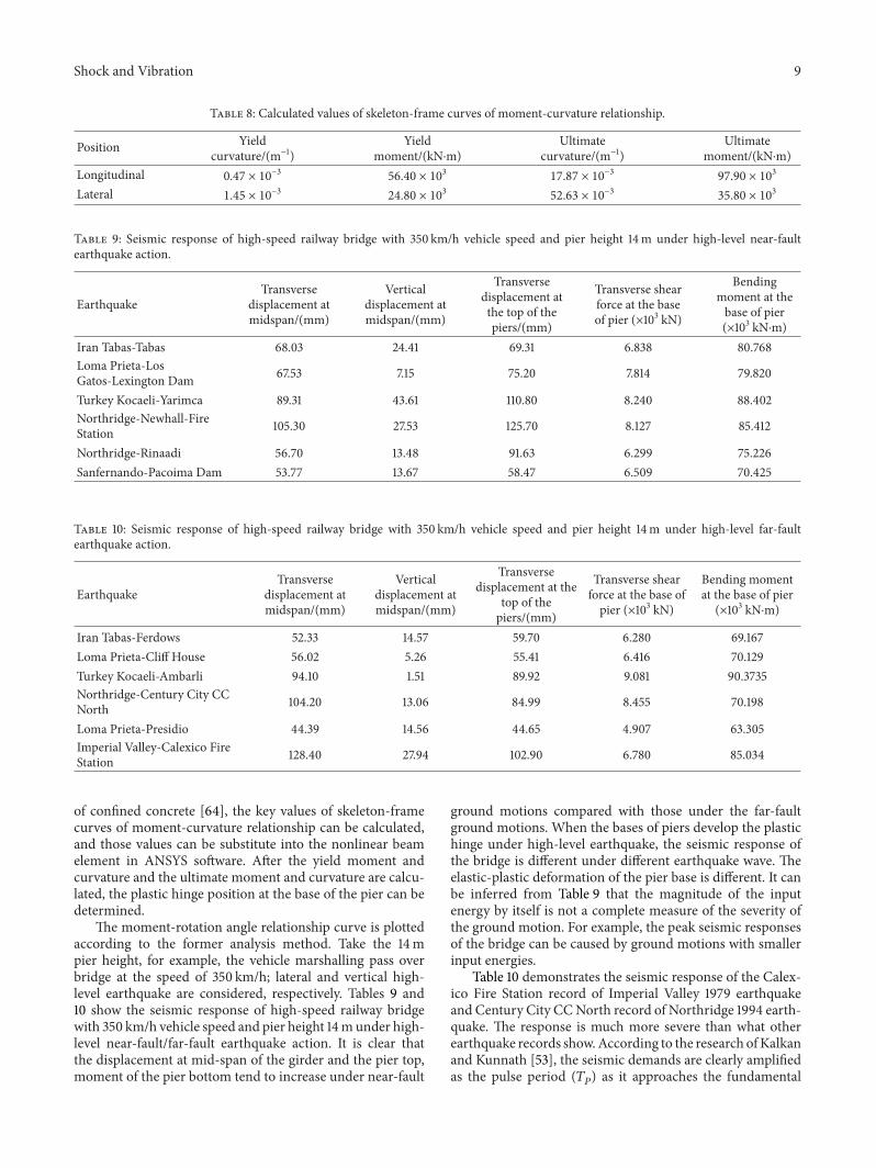
Table 8: Calculated values of skeleton-frame curves of moment-curvature relationship.

Position Yieldcurvature/(m−1)

Yieldmoment/(kN⋅m)

Ultimatecurvature/(m−1)

Ultimatemoment/(kN⋅m)

Longitudinal 0.47 × 10−3

56.40 × 103

17.87 × 10−3

97.90 × 103

Lateral 1.45 × 10−3

24.80 × 103

52.63 × 10−3

35.80 × 103

Table 9: Seismic response of high-speed railway bridge with 350 km/h vehicle speed and pier height 14m under high-level near-faultearthquake action.

EarthquakeTransverse

displacement atmidspan/(mm)

Verticaldisplacement atmidspan/(mm)

Transversedisplacement atthe top of thepiers/(mm)

Transverse shearforce at the baseof pier (×103 kN)

Bendingmoment at thebase of pier(×103 kN⋅m)

Iran Tabas-Tabas 68.03 24.41 69.31 6.838 80.768Loma Prieta-LosGatos-Lexington Dam 67.53 7.15 75.20 7.814 79.820

Turkey Kocaeli-Yarimca 89.31 43.61 110.80 8.240 88.402Northridge-Newhall-FireStation 105.30 27.53 125.70 8.127 85.412

Northridge-Rinaadi 56.70 13.48 91.63 6.299 75.226Sanfernando-Pacoima Dam 53.77 13.67 58.47 6.509 70.425

Table 10: Seismic response of high-speed railway bridge with 350 km/h vehicle speed and pier height 14m under high-level far-faultearthquake action.

EarthquakeTransverse

displacement atmidspan/(mm)

Verticaldisplacement atmidspan/(mm)

Transversedisplacement at the

top of thepiers/(mm)

Transverse shearforce at the base ofpier (×103 kN)

Bending momentat the base of pier

(×103 kN⋅m)

Iran Tabas-Ferdows 52.33 14.57 59.70 6.280 69.167Loma Prieta-Cliff House 56.02 5.26 55.41 6.416 70.129Turkey Kocaeli-Ambarli 94.10 1.51 89.92 9.081 90.3735Northridge-Century City CCNorth 104.20 13.06 84.99 8.455 70.198

Loma Prieta-Presidio 44.39 14.56 44.65 4.907 63.305Imperial Valley-Calexico FireStation 128.40 27.94 102.90 6.780 85.034

of confined concrete [64], the key values of skeleton-framecurves of moment-curvature relationship can be calculated,and those values can be substitute into the nonlinear beamelement in ANSYS software. After the yield moment andcurvature and the ultimate moment and curvature are calcu-lated, the plastic hinge position at the base of the pier can bedetermined.

The moment-rotation angle relationship curve is plottedaccording to the former analysis method. Take the 14mpier height, for example, the vehicle marshalling pass overbridge at the speed of 350 km/h; lateral and vertical high-level earthquake are considered, respectively. Tables 9 and10 show the seismic response of high-speed railway bridgewith 350 km/h vehicle speed and pier height 14munder high-level near-fault/far-fault earthquake action. It is clear thatthe displacement at mid-span of the girder and the pier top,moment of the pier bottom tend to increase under near-fault

ground motions compared with those under the far-faultground motions. When the bases of piers develop the plastichinge under high-level earthquake, the seismic response ofthe bridge is different under different earthquake wave. Theelastic-plastic deformation of the pier base is different. It canbe inferred from Table 9 that the magnitude of the inputenergy by itself is not a complete measure of the severity ofthe ground motion. For example, the peak seismic responsesof the bridge can be caused by ground motions with smallerinput energies.

Table 10 demonstrates the seismic response of the Calex-ico Fire Station record of Imperial Valley 1979 earthquakeand Century City CCNorth record of Northridge 1994 earth-quake. The response is much more severe than what otherearthquake records show.According to the research ofKalkanand Kunnath [53], the seismic demands are clearly amplifiedas the pulse period (𝑇𝑃) as it approaches the fundamental


−3.0 −2.0 −1.0 0.0 1.0 2.0 3.0

8.0

6.0

4.0

2.0

0.0

−2.0

−4.0

−6.0

−8.0

Mom

ent (×10

7N·m

)

Rotation angle (×10−3 rad)

(a) First element at the base of pier

−2.0 −1.5 −1.0 −0.5 0.0 0.5 1.0 1.58.0

6.0

4.0

2.0

0.0

−2.0

−4.0

−6.0

−8.0

Mom

ent (×10

7N·m

)


(b) Second element at the base of pier

−2.0 −1.5 −1.0 −0.5 0.0 0.5 1.0

6.0

4.0

2.0

0.0

−2.0

−4.0

−6.0

Mom

ent (×10

7N·m

)


(c) Third element at the base of pier

−0.8 −0.6 −0.4 −0.2 0.0 0.2 0.4 0.66.0

4.0

2.0

0.0

−2.0

−4.0

−6.0

Mom

ent (×10

7N·m

)


(d) Fourth element at the base of pier

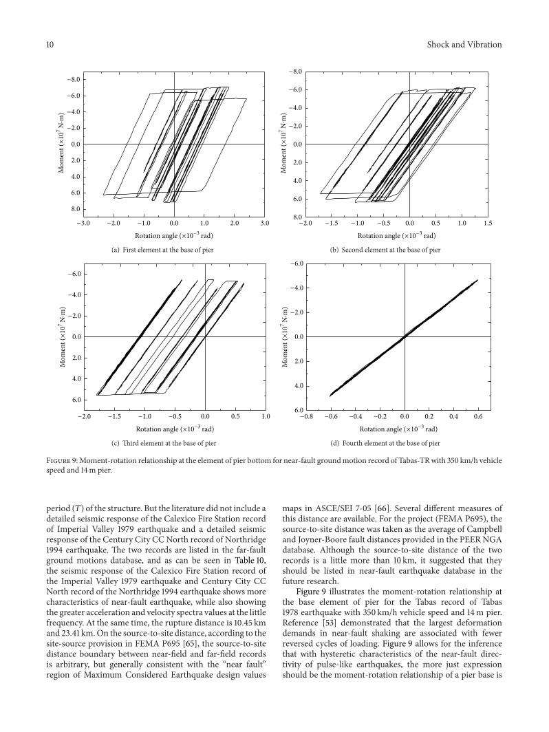
Figure 9:Moment-rotation relationship at the element of pier bottom for near-fault groundmotion record of Tabas-TRwith 350 km/h vehiclespeed and 14m pier.

period (𝑇) of the structure. But the literature did not include adetailed seismic response of the Calexico Fire Station recordof Imperial Valley 1979 earthquake and a detailed seismicresponse of the Century City CC North record of Northridge1994 earthquake. The two records are listed in the far-faultground motions database, and as can be seen in Table 10,the seismic response of the Calexico Fire Station record ofthe Imperial Valley 1979 earthquake and Century City CCNorth record of the Northridge 1994 earthquake shows morecharacteristics of near-fault earthquake, while also showingthe greater acceleration and velocity spectra values at the littlefrequency. At the same time, the rupture distance is 10.45 kmand 23.41 km.On the source-to-site distance, according to thesite-source provision in FEMA P695 [65], the source-to-sitedistance boundary between near-field and far-field recordsis arbitrary, but generally consistent with the “near fault”region of Maximum Considered Earthquake design values

maps in ASCE/SEI 7-05 [66]. Several different measures ofthis distance are available. For the project (FEMA P695), thesource-to-site distance was taken as the average of Campbelland Joyner-Boore fault distances provided in the PEER NGAdatabase. Although the source-to-site distance of the tworecords is a little more than 10 km, it suggested that theyshould be listed in near-fault earthquake database in thefuture research.

Figure 9 illustrates the moment-rotation relationship atthe base element of pier for the Tabas record of Tabas1978 earthquake with 350 km/h vehicle speed and 14m pier.Reference [53] demonstrated that the largest deformationdemands in near-fault shaking are associated with fewerreversed cycles of loading. Figure 9 allows for the inferencethat with hysteretic characteristics of the near-fault direc-tivity of pulse-like earthquakes, the more just expressionshould be the moment-rotation relationship of a pier base is


−3.0 −2.0 −1.0 0.0 1.0

6.0

4.0

2.0

0.0

−2.0

−4.0

−6.0

Mom

ent (×10

7N·m

)



−1.0 −0.6 −0.2 0.2 0.6 1.0

6.0

4.0

2.0

0.0

−2.0

−4.0

−6.0

Mom

ent (×10

7N·m

)



−0.6 −0.4 −0.2 0.0 0.2 0.4 0.66.0

4.0

2.0

0.0

−2.0

−4.0

−6.0

Mom

ent (×10

7N·m

)



Figure 10: Moment-rotation relationship at the element of pier bottom for far-fault ground motion record of Tabas-FER-T1 with 350 km/hvehicle speed and 14m pier.

0 1 2 3 40

20406080

100120140160180200220240

Spec

tral

vel

ocity

(cm

/s)

Period (s)

YarimcaLexington DamRinaldi

Fire stationPacoima DamTabas TR 3

𝜉 = 0.5%

Figure 11: Velocity spectra of near-fault ground motions.


0 1 2 3 40

102030405060708090

100

CalexicoFerdowAmbarl

PresidioCliff HouseCCC North

Period (s)

Spec

tral

vel

ocity

(cm

/s)

𝜉 = 0.5%

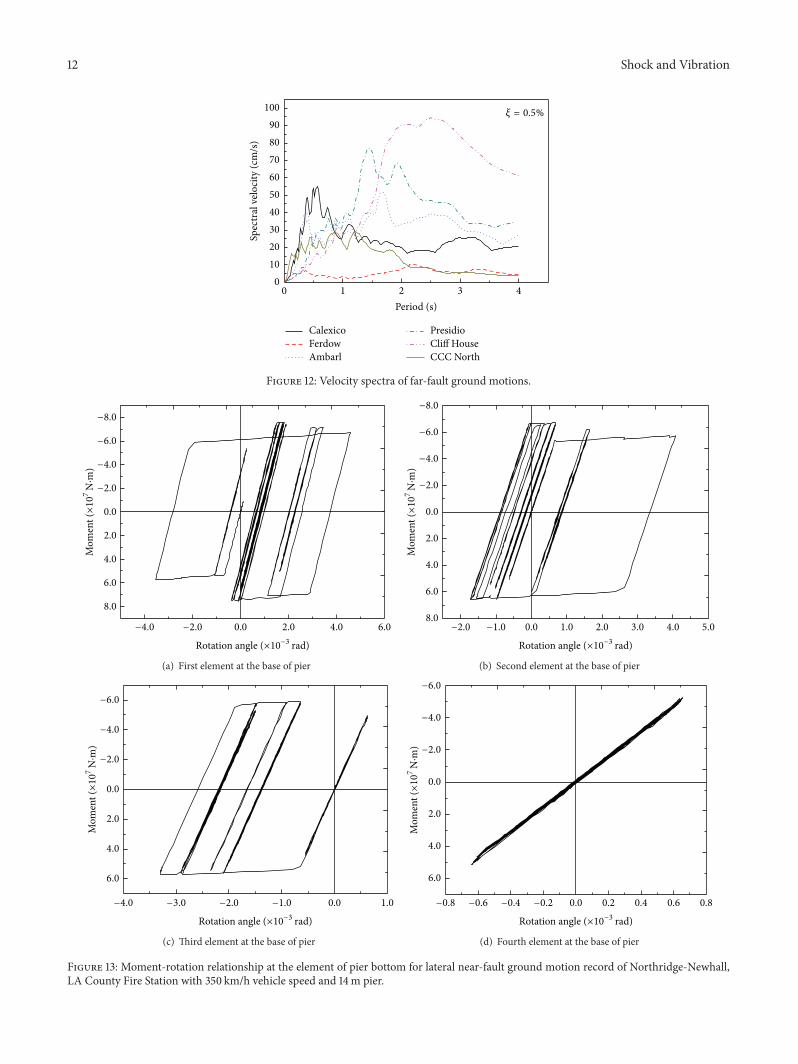
Figure 12: Velocity spectra of far-fault ground motions.

−4.0 −2.0 0.0 2.0 4.0 6.0

8.0

6.0

4.0

2.0

0.0

−2.0

−4.0

−6.0

−8.0

Mom

ent (×10

7N·m

)



−2.0 −1.0 0.0 1.0 2.0 3.0 4.0 5.08.0

6.0

4.0

2.0

0.0

−2.0

−4.0

−6.0

−8.0M

omen

t (×10

7N·m

)



−4.0 −3.0 −2.0 −1.0 0.0 1.0

6.0

4.0

2.0

0.0

−2.0

−4.0

−6.0

Mom

ent (×10

7N·m

)



−0.8 −0.6 −0.4 −0.2 0.0 0.2 0.4 0.6 0.8

6.0

4.0

2.0

0.0

−2.0

−4.0

−6.0

Mom

ent (×10

7N·m

)



Figure 13: Moment-rotation relationship at the element of pier bottom for lateral near-fault ground motion record of Northridge-Newhall,LA County Fire Station with 350 km/h vehicle speed and 14m pier.


−6.0 −5.0 −4.0 −3.0 −2.0 −1.0 0.0 1.0

8.0

6.0

4.0

2.0

0.0

−2.0

−4.0

−6.0

−8.0

Mom

ent (×10

7N·m

)



−1.0 −0.5 0.0 0.5 1.0 1.5 2.0 2.5 3.0 3.58.0

6.0

4.0

2.0

0.0

−2.0

−4.0

−6.0

−8.0

Mom

ent (×10

7N·m

)



−1.5 −1.0 −0.5 0.0 0.5 1.0

6.0

4.0

2.0

0.0

−2.0

−4.0

−6.0

Mom

ent (×10

7N·m

)



−0.6 −0.4 −0.2 0.0 0.2 0.4 0.66.0

4.0

2.0

0.0

−2.0

−4.0

−6.0

Mom

ent (×10

7N·m

)



Figure 14: Moment-rotation relationship at the element of pier bottom for lateral near-fault ground motion record of Northridge-Rinaadistation with 350 km/h vehicle speed and 14m pier.

characterized by the central strengthened hysteretic cycles. Atsome point of the loading time-history curve correspondingto the time of the pulse, this is due to the dissipation of suddenenergy in a short period of time in a single or few excursions.It requires the bridge piers to dissipate considerable inputenergy in a single or relatively few plastic cycles, meaning thatthe ductility capacity of the piers should be improved.

On the other hand, as can be shown in Figure 10which illustrates the moment-rotation relationship at thebase element of pier for the Ferdows record of the Tabas1978 earthquake with 350 km/h vehicle speed and 14m pier,the energy dissipation on the bridge system subjected to afar-fault motion tends to gradually increase over a longerduration, causing an incremental build-up of input energy.As is shown in Figure 9, followed by several cycles of elasticaction, the consequence of a single predominant peak isa well-pronounced permanent offset displacement, and the

subsequent response is essentially a series of elastic cyclesabout this deformed configuration.

To put the severity of near-fault ground motions inperspective with the severity of ground motions representedby current codes, the velocity spectra of near-fault groundmotions are presented in the study with given a dampingratio of 𝜉 = 5%. Although some of the records have morethan one clear velocity peak, an important observation fromthe near-fault spectra (Figures 11 and 12) is the existenceof a predominant peak in the velocity spectrum of most ofthe near-fault records. The predominant peak of the velocityspectrum is used to later estimate the period of the pulsecontained in the near-fault record.

Figure 11 illustrates the velocity spectra of 6 recordednear-fault time histories. This figure is presented for two rea-sons: to illustrate the great variability in near-fault responsespectra and second and to put the severity of near-fault


ground motions in perspective with the severity of groundmotions represented by current codes. The velocity spectraof a reference set of 6 far-fault ground motions recordsare presented in Figure 12. The velocity spectra value ofnear-fault ground motions is greater when the period offar-fault ground motions is within 3 sec, and the velocityspectra value is greater when the period exceeds 3 sec. Thisis significant to railway simply supported bridges which haveshort foundational periods.

Vertical ground motion component is not consideredexplicitly in the design of ordinary bridges. A comparisonanalysis of vertical ground motion effects is presented in thestudy to evaluate the vertical ground motion effects on theresponse of the high-speed railway bridges. Plastic hingesowing to the vertical acceleration are expected at the pierbottom where an amplification of the vertical motion isalso expected to depend on the high value of the verticalacceleration, and the spacing of the hysteresis hoops is largeand can be manifested in the moment-rotation relationshipat the element of pier bottom for lateral near-fault groundmotion record of the Northridge-Newhall, LA County FireStation, and Northridge-Rinaadi station in Figures 13 and14.

Since Newmark et al. [67] suggested that the average peakvertical-to-horizontal spectral ratio 𝜕PGA can reasonably betaken as 2/3, almost all modem codes accept the value and useit to scale down the horizontal spectrum and consequentlyarrive at a vertical spectrum. This implies that the vertical-to-horizontal PGA ratio 𝜕PGA is also 2/3 assuming constantamplification. Whereas the latter study is based on a ratherlimited dataset of 33 components and uses it so as toscale down the horizontal spectrum in order to arrive ata vertical spectrum. However, there is strong evidence thatthe 𝜕PGA value of the V/H ratio is unconservative in thenear-fault ground motion [68]. According to the site naturalperiod, rupture distance, and the site properties, the 𝜕PGAvalue should be revised in the future research, while thediscreteness of 𝜕PGA should also be considered.

6. Summary

The study summarized in this paper addresses the nonlinearseismic response characteristics of high-speed railway bridgestructures that are subjected to near-fault FD pulse-likeground motions. A procedure for estimating the effects ofFD pulse on the seismic response of high-speed railwaybridge is introduced based on the PEER NAG strong groundmotion database. The VTB element is presented to simulatethe interaction between a train and a bridge. A train ismodeled as a series of sprung masses concentrated at the axlepositions, while the effects of the high values of the verticalaccelerations are taken into consideration. It is emphasizedthat the conclusions and results presented in this paper areapplicable only within the context of the assumptions made.The conclusions of this study are summarized for the shortperiod railway bridge (𝑇 ≤ 𝑇𝑃), as subjected to near-fault FDpulse-like ground motions as follows.

(1) The directivity pulse effect tends to increase thedisplacement response of the girder and pier top,moment response of the pier bottom in inelastichigh-speed railway bridge relative to far-fault groundmotion or nonpulse-like motions. These displace-ment demandsmay increase structural and nonstruc-tural damage.

(2) The largest deformation demands in near-fault direc-tivity pulse-like ground motions shaking are associ-ated with fewer reversed cycles of loading. In regardto the hysteretic characteristics of the near-faultdirectivity pulse-like earthquake, the expression usedshould be the moment-rotation relationship of pierbottom is characterized by the central strengthenedhysteretic cycles at some point of the loading time-history, which may be corresponding to the time ofthe pulse. It requires that the bridge piers to dissipateconsiderable input energy in a single or relatively fewplastic cycles.Thismeans that the ductility capacity ofthe piers should be improved.

(3) As the high values of the acceleration ratio 𝜕PGA areinvolved in near-fault ground motions, there are thelarge vertical deflections in the midspan of girder;therefore, high values of 𝜕PGA can notably modify theaxial load in the bridge piers. This can influence thehysteretic behavior; for example, the spacing of thehysteresis hoops is large; the constant amplification𝜕PGA is taken as 2/3 bymost of codes is unconservativein the near-fault ground motion. According to thesite natural period, rupture distance, and the siteproperties, the 𝜕PGA value should be revised, and thediscreteness of the 𝜕PGA should be considered.

Conflict of Interests

The authors declare that there is no conflict of interestsregarding the publication of this paper.

Acknowledgments

The research summarized in this paper was supported bythe Major State Basic Research Development Program ofChina (“973” Program) through Grant no. 2013CB036203,China Postdoctoral Science Foundation through Grant no.2013M530022, Science and Technology Plan Projects ofMinistry of Housing and Urban-Rural Development of thePeople’s Republic of China through Grant no. 2013-K5-31,High-Level Scientific Research Foundation for the introduc-tion of talent of Yangzhou University, the Open Fund of theNational Engineering Laboratory for High Speed RailwayConstruction, the Program for Changjiang Scholars andInnovative Research Team in University “PCSIRT” Projectthrough Grant no. IRT1296), and National Natural ScienceFoundation of China through Grant no. 50908236. Thissupport is gratefully acknowledged.


References

[1] P. G. Somerville, N. F. Smith, R. W. Graves, and N. A.Abrahamson, “Modification of empirical strong groundmotionattenuation relations to include the amplitude and durationeffects of rupture directivity,” Seismological Research Letters, vol.68, no. 1, pp. 199–222, 1997.

[2] H. Benioff, “Mechanism and strain characteristics of the WhiteWolf fault as indicated by the aftershock sequence,” in Earth-quakes inKernCounty, California during 1952, Author’s Separate,Part II Seismology, Bulletin 171, pp. 199–200, California Depart-ment of Natural Resources, Division of Mines, 1955.

[3] K. Kasahara, “An attempt to detect azimuth effect on spectralstructures of seismicwaves: the Alaskan earthquakes of April 7,1958,” Bulletin of the Earthquake Research Institute, vol. 38, no.2, pp. 207–218, 1960.

[4] N. A. Haskell, “Total energy and energy spectral density ofelastic wave radiation from propagating faults,” Bulletin of theSeismological Society of America A, vol. 54, no. 6, pp. 1811–1842,1964.

[5] A. Ben-Menahem, “Radiation of seismic surface-waves fromfinite moving sources,” Bulletin of the Seismological Society ofAmerica, vol. 51, no. 3, pp. 401–435, 1961.

[6] T. H. Heaton, “The 1971 San Fernando earthquake; a doubleevent?” Bulletin of the Seismological Society of America A, vol.72, no. 6, pp. 2037–2062, 1982.

[7] D. M. Boore and R. L. Porcella, “Peak horizontal groundmotions from the 1979 Imperial valley earthquake: comparisonwith data from previous earthquakes,” in Selected Papers onthe Imperial Valley, California, Earthquake of October 15, 1979,R. Christopher, Ed., U.S. Geological Survey, Open-File Report,United States Department of the Interior, Geological Survey,Menlo Park, Calif, USA, 1980.

[8] D. J. Wald, T. H. Heaton, and K.W. Hudnut, “The slip history ofthe 1994 Northridge, California, earthquake determined fromstrong-motion, teleseismic, GPS, and leveling data,” Bulletin ofthe Seismological Society of America B, vol. 86, no. 1, pp. S49–S70, 1996.

[9] Y.-G. Li, K. Aki, J. E. Vidale, andM.G. Alvarez, “A delineation ofthe Nojima fault ruptured in the M7.2 Kobe, Japan, earthquakeof 1995 using fault zone trapped waves,” Journal of GeophysicalResearch B, vol. 103, no. 4, pp. 7247–7263, 1998.

[10] W.-C. Chi, D. Dreger, andA. Kaverina, “Finite-sourcemodelingof the 1999 Taiwan (Chi-Chi) earthquake derived from a densestrong-motion network,” Bulletin of the Seismological Society ofAmerica, vol. 91, no. 5, pp. 1144–1157, 2001.

[11] S. W. Park, H. Ghasemi, J. Shen, P. G. Somerville, W. P. Yen,and M. Yashinsky, “Simulation of the seismic performanceof the Bolu Viaduct subjected to near-fault ground motions,”Earthquake Engineering & Structural Dynamics, vol. 33, no. 13,pp. 1249–1270, 2004.

[12] B. Alavi and H. Krawinkler, “Consideration of near-faultground motion effects in seismic design,” in Proceedings of the12th World Conference on Earthquake Engineering, Paper no.2665, 2000.

[13] H. Choi, M. Saiidi, P. G. Somerville, and S. S. El-Azazy,“Bridge seismic analysis procedure to address near-fault effects,”in Proceedings Caltrans Bridge Research Conference, Califor-nia Transportation Foundation and California Department ofTransportation, Sacramento, Calif, USA, 2005.

[14] A. Mortezaei and H. R. Ronagh, “Plastic hinge length ofreinforced concrete columns subjected to both far-fault and

near-fault ground motions having forward directivity,” TheStructural Design of Tall and Special Buildings, vol. 22, no. 12,pp. 903–926, 2013.

[15] G. A. MacRae, D. V. Morrow, and C. W. Roeder, “Near-fault ground motion effects on simple structures,” Journal ofStructural Engineering, vol. 127, no. 9, pp. 996–1004, 2001.

[16] P. Tothong and C. A. Cornell, “Structural performance assess-ment under near-source pulse-like ground motions usingadvanced groundmotion intensitymeasures,” Earthquake Engi-neering& Structural Dynamics, vol. 37, no. 7, pp. 1013–1037, 2008.

[17] J.W.Baker andC.A.Cornell, “Vector-valued intensitymeasuresfor pulse-like near-fault ground motions,” Engineering Struc-tures, vol. 30, no. 4, pp. 1048–1057, 2008.

[18] L. Xu, A. Rodriguez-Marek, and L. Xie, “Design spectra includ-ing effect of rupture directivity in near-fault region,” EarthquakeEngineering and Engineering Vibration, vol. 5, no. 2, pp. 159–170,2006.

[19] E. Chioccarelli and I. Iervolino, “Near-source seismic demandand pulse-like records: a discussion for L’Aquila earthquake,”Earthquake Engineering & Structural Dynamics, vol. 39, no. 9,pp. 1039–1062, 2010.

[20] F. Mazza and A. Vulcano, “Nonlinear dynamic response ofr.c. framed structures subjected to near-fault ground motions,”Bulletin of Earthquake Engineering, vol. 8, no. 6, pp. 1331–1350,2010.

[21] L.-K. Chen, L.-Z. Jiang, L.-P. Wang, and B.-F. Luo, “Analysisof elastoplastic seismic response of high-speed railway bridgewith round-ended piers,” Journal of South China University ofTechnology, vol. 39, no. 6, pp. 126–131, 2011 (Chinese).

[22] L.-K. Chen, L.-Z. Jiang, Z.-W. Yu, and Z.-P. Zeng, “Studyon earthquake characteristics of high-speed railway simply-supported girder bridge,” Journal of Vibration and Shock, vol.30, no. 12, pp. 216–222, 2011 (Chinese).

[23] L. K. Chen, L. Z. Jiang, and Z. Zeng, “Numerical analysis ofseismic responses of high-speed railway bridge round-endedpiers,” Journal of Hunan University Natural Sciences, vol. 39, no.4, pp. 19–25, 2012 (Chinese).

[24] L. K. Chen, L. Z. Jiang, Z. P. Zeng, andW. G. Long, “Numericalmodeling and simulation on seismic performance of high-speed railway bridge system,” Noise and Vibration Worldwide,vol. 42, no. 10, pp. 15–22, 2011.

[25] B. Alavi and H. Krawinkler, “Behavior of moment-resistingframe structures subjected to near-fault ground motions,”Earthquake Engineering & Structural Dynamics, vol. 33, no. 6,pp. 687–706, 2004.

[26] W.-I. Liao, C.-H. Loh, and B.-H. Lee, “Comparison of dynamicresponse of isolated and non-isolated continuous girder bridgessubjected to near-fault groundmotions,”Engineering Structures,vol. 26, no. 14, pp. 2173–2183, 2004.

[27] W.-I. Liao, C.-H. Loh, S. Wan, W.-Y. Jean, and J.-F. Chai,“Dynamic responses of bridges subjected to near-fault groundmotions,” Journal of Chinese Institute of Engineering, vol. 23, no.4, pp. 455–464, 2000.

[28] Z. Gulerce, E. Erduran, S. K. Kunnath, and N. A. Abrahamson,“Seismic demand models for probabilistic risk analysis ofnear fault vertical ground motion effects on ordinary highwaybridges,” Earthquake Engineering & Structural Dynamics, vol.41, no. 2, pp. 159–175, 2012.

[29] Y. Z. Ju, G. P. Yan, and L. Liu, “Experimental study onseismic behaviors of large-scale RC round-ended piers with lowreinforcement ratio,” China Civil Engineering Journal, vol. 36,no. 11, pp. 66–69, 2003 (Chinese).


[30] J. Shen, M.-H. Tsai, K.-C. Chang, and G. C. Lee, “Performanceof a seismically isolated bridge under near-fault earthquakeground motions,” ASCE Journal of Structural Engineering, vol.130, no. 6, pp. 861–868, 2004.

[31] G. L. Dai,W. S. Liu, and L. Y. Li, “Study of the live load for small-and medium-span bridges of high-speed railways,” China CivilEngineering Journal, vol. 45, no. 10, pp. 161–168, 2012 (Chinese).

[32] N. Zhang and H. Xia, “Dynamic analysis of coupled vehicle-bridge system based on inter-system iteration method,” Com-puters & Structures, vol. 114-115, pp. 26–34, 2013.

[33] M. M. Gao and J. Y. Pan, “Coupling vibration analysis fortrain-track-bridge system,” in Proceedings of the 6th EuropeanConference on Structural Dynamics (EURODYN ’05), Paris,France, 2005.

[34] X. Z. Li,W. B.Ma, and S. Z. Qiang, “Coupling vibration analysisof vehicle-bridge system by iterative solution method,” Journalof Vibration and Shock, vol. 21, no. 3, pp. 21–25, 2002 (Chinese).

[35] J.-S. Jo, H.-J. Jung, and H. Kim, “Finite element analysis ofvehicle-bridge interaction by an iterative method,” StructuralEngineering & Mechanics, vol. 30, no. 2, pp. 165–176, 2008.

[36] Y. B. Yang and Y. S. Wu, “A versatile element for analyzingvehicle-bridge interaction response,” Engineering Structures,vol. 23, no. 5, pp. 452–469, 2001.

[37] Y. K. Cheung, F. T. K. Au, D. Y. Zheng, and Y. S. Cheng,“Vibration of multispan non-uniform bridges under movingvehicles and trains by usingmodified beamvibration functions,”Journal of Sound andVibration, vol. 228, no. 3, pp. 611–628, 1999.

[38] H. Xia, Y. Han, N. Zhang, and W. W. Guo, “Dynamic analysisof train-bridge system subjected to non-uniform seismic exci-tations,”Earthquake Engineering& Structural Dynamics, vol. 35,no. 12, pp. 1563–1579, 2006.

[39] J. C. O. Nielsen and T. J. S. Abrahamsson, “Coupling of physicaland modal components for analysis of moving non-lineardynamic systems on general beam structures,” InternationalJournal for Numerical Methods in Engineering, vol. 33, no. 9, pp.1843–1859, 1992.

[40] J.-D. Yau, Y.-B. Yang, and S.-R. Kuo, “Impact response of highspeed rail bridges and riding comfort of rail cars,” EngineeringStructures, vol. 21, no. 9, pp. 836–844, 1999.

[41] C. Jiang and Z. M. Lin, “Test and research on the ballast-freetrack structure for high-speed railway,” Chinese Railways, vol. 7,pp. 22–24, 2000 (Chinese).

[42] E. S. Hwang and A. S. Nowak, “Simulation of dynamic load forbridges,” ASCE Journal of Structural Engineering, vol. 117, no. 5,pp. 1413–1434, 1991.

[43] F. Yang and G. A. Fonder, “An iterative solution methodfor dynamic response of bridge-vehicles systems,” EarthquakeEngineering & Structural Dynamics, vol. 25, no. 2, pp. 195–215,1996.

[44] L. K. Chen, Seismic responses of high-speed railway train-ballastless track-bridge system and train-running safety duringearthquake [Ph.D. thesis], Central South University, Changsha,China, 2012, (Chinese).

[45] L. K. Chen, L. Z. Jiang, and P. Liu, “Seismic response analysesof high-speed railway bridge round-ended piers using globalbridge model,” International Journal of Materials and ProductTechnology, vol. 44, no. 1-2, pp. 35–46, 2012.

[46] Q. Fu and C. Menun, “Seismic-environment-based simulationof near-fault ground motions,” in Proceedings of the 13th WorldConference on Earthquake Engineering, Vancouver, Canada,2004.

[47] S. Akkar, U. Yazgan, and P. Gulkan, “Drift estimates in framebuildings subjected to near-fault ground motions,” Journal ofStructural Engineering, vol. 131, no. 7, pp. 1014–1024, 2005.

[48] J. W. Baker, “Quantitative classification of near-fault groundmotions using wavelet analysis,” Bulletin of the SeismologicalSociety of America, vol. 97, no. 5, pp. 1486–1501, 2007.

[49] F. Mazza and A. Vulcano, “Effects of near-fault ground motionson the nonlinear dynamic response of base-isolated r.c. framedbuildings,” Earthquake Engineering & Structural Dynamics, vol.41, no. 2, pp. 211–232, 2012.

[50] Federal Emergency Management Agency, NEHRP Recom-mended Provisions for Seismic Regulations for NewBuildings andOther Structures, FEMA 450, FEMA, Washington, DC, USA,2003.

[51] B. Alavi and H. Krawinkler, “Effects of near-fault groundmotions on frame structures,” John A. Blume EarthquakeEngineering Center Report 138, Stanford University, 2001.

[52] Pacific Earthquake Engineering Center (PEER), “PEER StrongGround Motion Database,” http://peer.berkeley.edu/products/strong ground motion db.html.

[53] E. Kalkan and S. K. Kunnath, “Effects of fling step and forwarddirectivity on seismic response of buildings,” Earthquake Spec-tra, vol. 22, no. 2, pp. 367–390, 2006.

[54] A. J. Papazoglou and A. S. Elnashai, “Analytical and fieldevidence of the damaging effect of vertical earthquake groundmotion,” Earthquake Engineering & Structural Dynamics, vol.25, no. 10, pp. 1109–1137, 1996.

[55] D. Benedetti and P. Carydis, “Influence of the vertical com-ponent on damage during shallow—near field earthquakes,”European Earthquake Engineering, vol. 3, pp. 3–12, 1999.

[56] F. Mazza and A. Vulcano, “Nonlinear dynamic response ofr.c. framed structures subjected to near-fault ground motions,”Bulletin of Earthquake Engineering, vol. 8, no. 6, pp. 1331–1350,2010.

[57] F.Mollaioli, A. Lucchini, Y.Cheng, andG.Monti, “Cheng andG.Monti, Intensity measures for the seismic response predictionof base-isolated buildings,” Bulletin of Earthquake Engineering,vol. 11, no. 5, pp. 1841–1866, 2013.

[58] GB 50011-2001, Code for Seismic Design of Building, ChinaArchitecture and Building Press, Beijing, China, 2008, (Chi-nese).

[59] GB 50011-2010, Code for Seismic Design of Buildings, ChinaBuilding Industry Press, Beijing, China, 2010, (Chinese).

[60] FEMA-356, Prestandard and Commentary for Seismic Rehabil-itation of Buildings, Federal Emergency Management Agency,Washington, DC, USA, 2000.

[61] J. Zheng, “Key technologies for high-speed railway bridgeconstruction,” Engineering Science, vol. 10, no. 7, pp. 18–27, 2008(Chinese).

[62] Temporary Provisions of Newly-Built 300-350km/H PassengerSpecial Railway Bridge Design[S], China Railway Press, Beijing,China, 2007, (Chinese).

[63] C. B. Chadwell, UCFYBER: Cross Section Analysis StructuralSoftware, Department of Civil and Environmental Engineering,University of California, Berkeley, Calif, USA, 1999.

[64] J. Mander, M. Priestley, and R. Park, “Theoretical stress-strain model for confined concrete,” ASCE Journal of StructuralEngineering, vol. 114, no. 8, pp. 1804–1826, 1988.

[65] FEMA, “Quantification of building seismic performance fac-tors,” FEMA P695, Applied Technology Council for the FederalEmergencyManagement Agency,Washington, DC, USA, 2009.


[66] ASCE, “Minimum design loads for buildings and other struc-tures,” ASCE/SEI 7-05, American Society of Civil Engineers,Reston, Va, USA, 2006.

[67] N. M. Newmark, J. A. Blume, and K. K. Kapur, “Seismic designspectra for nuclear power plants,” ASCE Journal of the PowerDivision , vol. 99, no. 2, pp. 287–303, 1973.

[68] A. S. Elnashai and A. J. Papazoglou, “Vertical earthquakeground motion: evidence, effects and simplified analysis pro-cedures,” ESEE 95-06, Civil Engineering Department, ImperialCollege, London, UK, 1995.

International Journal of

AerospaceEngineeringHindawi Publishing Corporationhttp://www.hindawi.com Volume 2014

RoboticsJournal of

Hindawi Publishing Corporationhttp://www.hindawi.com Volume 2014


Active and Passive Electronic Components

Control Scienceand Engineering

Journal of



RotatingMachinery


Hindawi Publishing Corporation http://www.hindawi.com

Journal ofEngineeringVolume 2014

Submit your manuscripts athttp://www.hindawi.com

VLSI Design



Shock and Vibration


Civil EngineeringAdvances in

Acoustics and VibrationAdvances in



Electrical and Computer Engineering

Journal of

Advances inOptoElectronics

Hindawi Publishing Corporation http://www.hindawi.com

Volume 2014

The Scientific World JournalHindawi Publishing Corporation http://www.hindawi.com Volume 2014

SensorsJournal of


Modelling & Simulation in EngineeringHindawi Publishing Corporation http://www.hindawi.com Volume 2014


Chemical EngineeringInternational Journal of Antennas and

Propagation




Navigation and Observation



DistributedSensor Networks


Research Article The Seismic Response of High-Speed...

Documents

Transcript of Research Article The Seismic Response of High-Speed...