1 | P a g e

Effects of ASEAN-Indian Free Trade agreements on Agriculture

Trade: Evidence from Augmented Gravity Model

Subhash Jagdambe, PhD Scholar, ADRTC, ISEC, Bangalore

Shjagdambe@gmail.com/ jagdambe@isec.ac.in

Abstract

The world is witnessing a rapid spread of economic regionalization, especially in the last 25

years. Regionalization is taking place through the formation of Free Trade Agreement (FTA).

The prime objective of the paper is to analyses the effects of ASEAN-India Free Trade

Agreement on agriculture trade. It cover ten years of data from 2005 to 2014 i.e. five years

pre and five years post-ASIAN-India FTA (AIFTA) period. Bilateral agricultural Trade data

compiled from World Trade Integration Solution and Gross Domestic product, per capita

GDP and Population data are taken from world Development Indicator published by World

Bank. The paper evaluates agricultural trade creation and diversion effects of major FTAs.

Trade creation and diversion effects are estimated using an augmented gravity model with

various fixed effects to control heterogeneity. The paper estimate the trade creation and trade

diversion effect for agricultural trade using intra and extra dummy variable. The paper found

clearly the trade creation effect for AFITA members. The result reveal that intraregional

agricultural trade among AIFTA members increase by 219 % [exp (1.16)-1)*100] more than

they traded with rest of the world. The Paper also found strong trade diversion effect for

MERCOSURE and EU15 over the study period. The result supports the argument that, the

FTAs is positive path towards freer multilateral trade. In nut shell the FTA has significant

and positive impact on bilateral agricultural trade among members during the study period.

Key words: Agriculture, FTA, Trade creation and Trade Diversion.

******

Introduction

The world is witnessing rapid spread of economic regionalism, especially in the last 25 years.

Regionalism is taking place through the formation of Free Trade Agreement (FTA). It would

reflect that, every month brings news of yet another agreement among a group of countries,

or between one group and another (Frankel, et. al. 1997). The number of FTAs has been

2 | P a g e

increasing steadily after the World Trade Organization (WTO) came into existence in 1995.

For instance, from 1948 to 1994 there were only 124 FTAs have been notified to the General

Agreement on Tariff and Trade (GATT), subsequently over 400 additional FTAs covering

trade in goods and services have been notified to the WTO/GATT. Out of which 300 FTAs

are in force and the remaining are in process in the year 20151. Basically, FTAs are form to

increase economic strength through removing barriers to trade and investment among

members. However, these FTAs had a controversial role in moving towards multilateralism.

Some argued that it hampering to multilateral trade negotiation (Levy 1997), and others say

that FTAs are positive path towards freer multilateral trade (Freund 2000).

The economist have debated long on this issues, whether FTAs are benefited to the countries

included in FTAs and on the rest of the world (Bhagwati and Krueger 1995). The debate

divided between those who support FTAs and those who oppose them. The former group

supported the Trade Creation (TC) effect of FTAs and latter supported the Trade Diversion2

(TD) effect of FTAs. The former group emphasised that TC effect outweighed the TD effect.

According to them, FTAs can improve recourse allocation and improve income among

members through reducing trade barriers. As well as, the production will also shift towards

most efficient producers and consumer will be better off because they can purchase goods at

lower price. Overall FTAs are welfare improving for members as well as the rest of the

world. The latter group are emphasis on TD effect of FTAs. By definition FTAs are

discriminatory in nature because members will grant preference among themselves while

retaining the barriers to non-members. Hence, the extent of these TC and TD effects is an

empirical question. Moreover, this study focuses on the effect of FTAs on agriculture trade

creation and trade diversion effect.

Literature Review

This section provides a brief overview of selected studies pertaining to trade analysis using

gravity model. Reviews divided in two parts, first part discuss with impact of FTAs on

overall trade flows and second parts only agriculture trade flows.

1 http://rtais.wto.org/UP/PublicMaintainRTAHome.aspx.

2 In general, trade creation means that a free trade area creates trade that would not have existed

otherwise. As a result, supply occurs from a more efficient producer of the product. On the other hand,

trade diversion means that a free trade area diverts trade, away from a more efficient supplier outside the

FTA, towards a least efficient supplier within the FTA (Suranovic, S. M.2010)

3 | P a g e

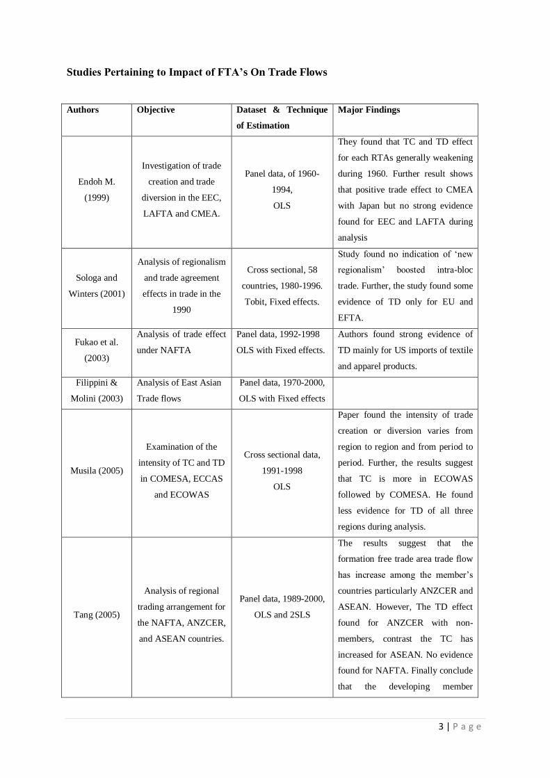
Studies Pertaining to Impact of FTA’s On Trade Flows

Authors Objective Dataset & Technique

of Estimation

Major Findings

Endoh M.

(1999)

Investigation of trade

creation and trade

diversion in the EEC,

LAFTA and CMEA.

Panel data, of 1960-

1994,

OLS

They found that TC and TD effect

for each RTAs generally weakening

during 1960. Further result shows

that positive trade effect to CMEA

with Japan but no strong evidence

found for EEC and LAFTA during

analysis

Sologa and

Winters (2001)

Analysis of regionalism

and trade agreement

effects in trade in the

1990

Cross sectional, 58

countries, 1980-1996.

Tobit, Fixed effects.

Study found no indication of ‘new

regionalism’ boosted intra-bloc

trade. Further, the study found some

evidence of TD only for EU and

EFTA.

Fukao et al.

(2003)

Analysis of trade effect

under NAFTA

Panel data, 1992-1998

OLS with Fixed effects.

Authors found strong evidence of

TD mainly for US imports of textile

and apparel products.

Filippini &

Molini (2003)

Analysis of East Asian

Trade flows

Panel data, 1970-2000,

OLS with Fixed effects

Musila (2005)

Examination of the

intensity of TC and TD

in COMESA, ECCAS

and ECOWAS

Cross sectional data,

1991-1998

OLS

Paper found the intensity of trade

creation or diversion varies from

region to region and from period to

period. Further, the results suggest

that TC is more in ECOWAS

followed by COMESA. He found

less evidence for TD of all three

regions during analysis.

Tang (2005)

Analysis of regional

trading arrangement for

the NAFTA, ANZCER,

and ASEAN countries.

Panel data, 1989-2000,

OLS and 2SLS

The results suggest that the

formation free trade area trade flow

has increase among the member’s

countries particularly ANZCER and

ASEAN. However, The TD effect

found for ANZCER with non-

members, contrast the TC has

increased for ASEAN. No evidence

found for NAFTA. Finally conclude

that the developing member

4 | P a g e

countries which having similar

income trade extensively more each

other

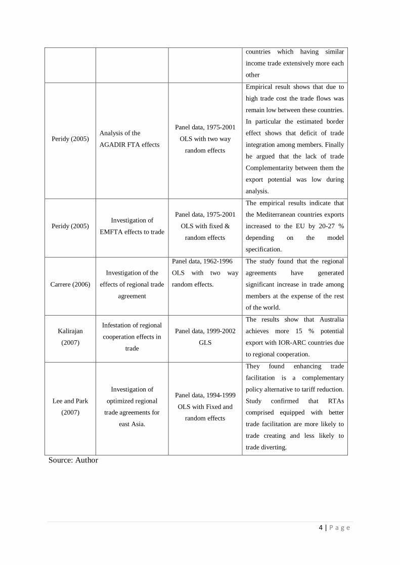
Peridy (2005) Analysis of the

AGADIR FTA effects

Panel data, 1975-2001

OLS with two way

random effects

Empirical result shows that due to

high trade cost the trade flows was

remain low between these countries.

In particular the estimated border

effect shows that deficit of trade

integration among members. Finally

he argued that the lack of trade

Complementarity between them the

export potential was low during

analysis.

Peridy (2005) Investigation of

EMFTA effects to trade

Panel data, 1975-2001

OLS with fixed &

random effects

The empirical results indicate that

the Mediterranean countries exports

increased to the EU by 20-27 %

depending on the model

specification.

Carrere (2006)

Investigation of the

effects of regional trade

agreement

Panel data, 1962-1996

OLS with two way

random effects.

The study found that the regional

agreements have generated

significant increase in trade among

members at the expense of the rest

of the world.

Kalirajan

(2007)

Infestation of regional

cooperation effects in

trade

Panel data, 1999-2002

GLS

The results show that Australia

achieves more 15 % potential

export with IOR-ARC countries due

to regional cooperation.

Lee and Park

(2007)

Investigation of

optimized regional

trade agreements for

east Asia.

Panel data, 1994-1999

OLS with Fixed and

random effects

They found enhancing trade

facilitation is a complementary

policy alternative to tariff reduction.

Study confirmed that RTAs

comprised equipped with better

trade facilitation are more likely to

trade creating and less likely to

trade diverting.

Source: Author

5 | P a g e

Studies Pertaining to Impact of FTA’s on Agriculture Trade Flows

In empirical research very few papers gave attention to an impact of FTAs on agricultural

trade flows among members. Among them Jayasinghe and Sarker (2008) estimate the TC and

TD effects of North American Free Trade Agreement (NAFTA) for six major agricultural

commodities. They found that intra-NAFTA trade has increased. But they did not point out

weather this increased as on the expense on rest of world. Another important study done by

Lambert and McKoy (2009), investigate the intra-and extra-bloc effects of FTAs on

agricultural and food products. They notice that generally members in FTAs increase

agricultural and food trade. For instance, NAFTA members’ agricultural trade has increased

by 145 % during analysis (trade creation effect). As well as they also notice trade diversion

effect for Caribbean Community and Common Market, the Central American Common

Market, the Andean Community, and the Common Market for Eastern and Southern Africa

(COMESA). The study by Lin and Reed (2010) estimate the impact of FTAs on member’s

agricultural trade. They found that ASEAN-China PTAs, EU-15, EU-25 and Southern

African Development Community (SADC) agreements have increased agricultural trade

among their members. There was significant export and import diversification from the EU-

15 but the creation of the SADC increased agricultural exports to non-member countries.

Less evidence found for trade creation among NAFTA but results support for export

diversion.

Overall very few studies focused on the impact of FTAs on agriculture trade. The reason is

that the agriculture sector has been excluded from most of the agreements. Since, the Doha

Round of development (2001)3, the agriculture sector got an important place in most of

FTAs. Earlier studies were consternated mostly only on NAFTA, EU etc. But no study has

found for ASEAN-India Free Trade Agreement (AIFTA). Hence, the present paper focused is

on the effect AIFTA on members’ agricultural trade using gravity model analysis.

GRAVITY MODEL SPECIFICATION

Jan Tinbergen (1962) was the first author applied gravity model to analyses international

trade. Since then the gravity model has became a ‘work-horse of international trade analysis

due to its explanatory power and it is commonly used in explaining the trade flows between

countries (Eichengreen and Irwin 1998). He shows that the size of bilateral trade flows

between any two countries can be approximated by a law called the “gravity equation” by

3 The agriculture sector was a cornerstone of Doha Round of WTO negotiation.

6 | P a g e

analogy with the Newtonian theory of gravitation4, countries trade in proportion to their

respective GDPs and proximity. Initially the gravity model was focused on stable relationship

between countries trade with their size of economise, and their distance. But international

trade theory at that time such as Ricardian and Heckscher-Ohlin (HO) theories relies on

difference in technology across countries and difference in factor endowments among

countries, respectively to explain trade pattern among the countries. These models were not

capable to provide a foundation for the gravity model. For instance, in HO theory country

size has little to do with the structure of trade flows.

Initially there was a lack of theoretical foundation for gravity model. To fill this gap the first

and foremost attempt was made by Anderson (1979). He assumed that where goods were

differentiated by country of origin (Armington assumption) and consumers have preference

defined over all the differentiated products. Subsequent, many others have explored the

theoretical determination of bilateral trade in which gravity equation were associated with

simple monopolistic competition model. In particular, Bergstrand (1985, 89), derived the

micro foundation for gravity model using general equilibrium approach. He used the utility

function to derive trade demand with income constraints, while trade supply is derived from

profit maximisation of firm in exporting country with resource allocation constraints. His

model is known as generalised gravity model because it included both price and income

terms.

The more appropriate theoretical rational related to the determination of bilateral trade

depends on GDP comes from work done by Helpman (1987), and Helpman and Krugman

(1985). They argued that, consumers have a preference for goods which they consumed,

products are differentiated by firm, not just by country, and firms are monopolistically

competitive. Further they said, the HO theory of comparative advantage does not have the

property that bilateral trade depends on the products on incomes, as it does in the gravity

model (Frankel, et.al. 1997).

Deardorff (1997) derived the gravity model from of HO theory as well as imperfect

competition. He incorporated the role of shipping cost as proxy for distance. More recently

Anderson and van Win coop (2003) derived gravity model based on constant Elasticity of

Substitution (CES) expenditure function that can be easily estimated. Further they shows that

4 According to Newton’s law of Gravity, the force between two masses is directly proportional to the product of

their size and inversely proportional to the square of the distance between them (Frankel, et.al. 1997).

7 | P a g e

bilateral trade is determined by relative trade cost, i.e. the propensity of country j to import

from country i is determined by country j trade cost toward i relative to its overall resistance

(average trade cost) to imports and to the average resistance facing exporter in rest of the

world.

Overall the theoretical argument that bilateral trade depend on the product of GDP, Frankel

et al (1997) also derived gravity model including imperfect substitutes and product

differentiation.

Traditional (Basic) Gravity Model

The basic gravity model is has multiplicative form as follows

𝑿𝒊𝒋 = 𝜶 Yi Yj / Distij (1)

Where, Xij is the monetary value of trade between i and j, Yi an Yj represents the income of

countries i and j respectively. Distij represent the distance between country i and j. It implies

that the bilateral trade between countries i and j is proportional to their respective income and

inverse to distance.

Standard Gravity Model

In basic gravity model only income and distance variable were included, while in standard

gravity model these tow variable and some more variable has incorporated like, common

border, common language and per capita income (Frankel 1197). The notation of the standard

gravity model explained in detail subsequent section.

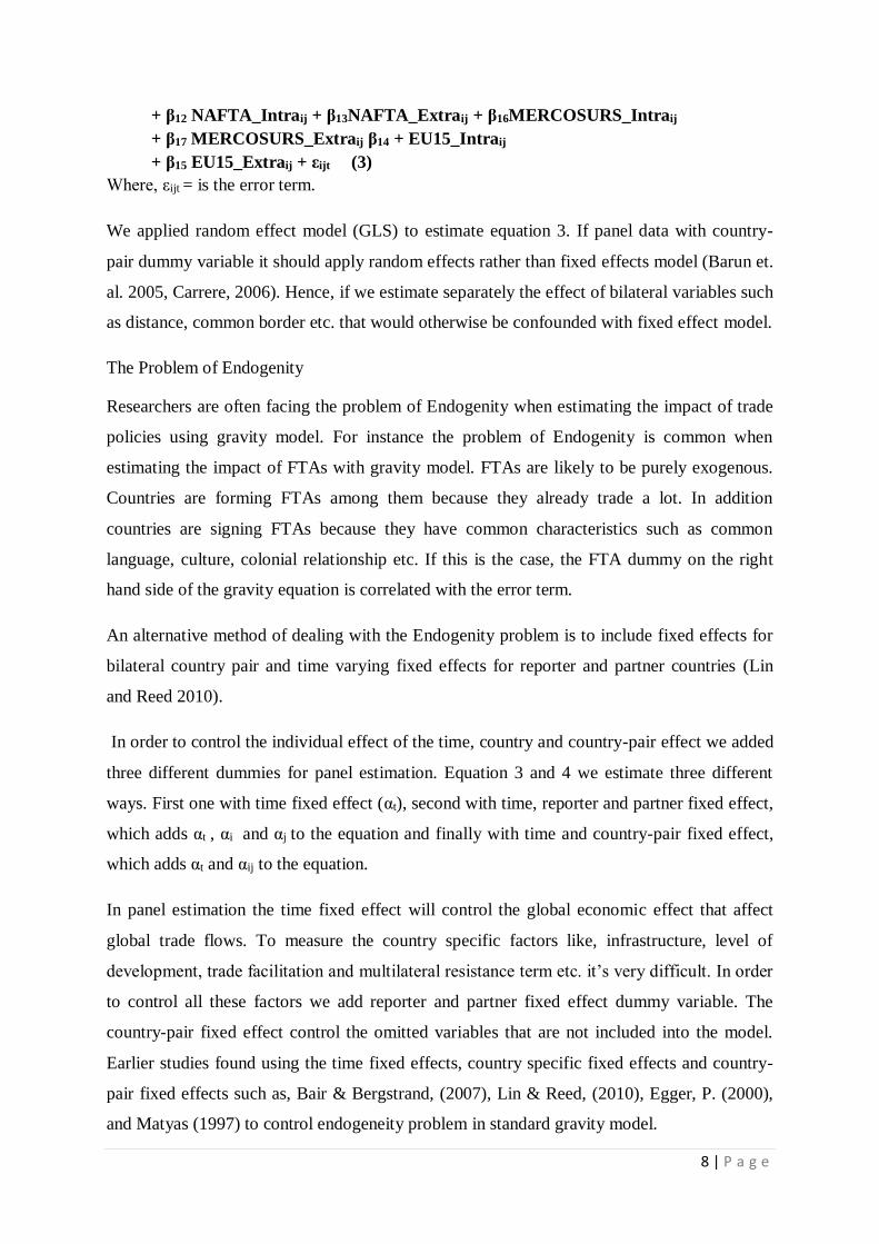
Framework for Estimation of Standard Gravity Model by a Panel Data regression

Model

We applied the following model for estimation proposes.

Xijt = α GDPit β1 GDPjt β2 POPit β3 POP jt

β4 Distij β6 eijt (2)

Where, Xijt is the bilateral trade (export plus import) between pairs5 of country i and country

j. All other variable are defined and expected sign are given table 1. Taking the logarithm of

equation (2) and incorporating the dummy variables listed in table 1.

lnXijt = β0 + β1 ln GDPit + β2ln GDPjt +β3ln POPit +β4 ln POP jt

+ β5 lnDistij + β6Comlij + β7Borderij + β8AIFTA_Intraij

+ β9 AIFTA_Extraij + β10 SAPTA_Intraij + β11 SAPTA_Extraij

5 The unit of observation is a pair of countries, not a single country.

8 | P a g e

+ β12 NAFTA_Intraij + β13NAFTA_Extraij + β16MERCOSURS_Intraij

+ β17 MERCOSURS_Extraij β14 + EU15_Intraij

+ β15 EU15_Extraij + εijt (3) Where, εijt = is the error term.

We applied random effect model (GLS) to estimate equation 3. If panel data with country-

pair dummy variable it should apply random effects rather than fixed effects model (Barun et.

al. 2005, Carrere, 2006). Hence, if we estimate separately the effect of bilateral variables such

as distance, common border etc. that would otherwise be confounded with fixed effect model.

The Problem of Endogenity

Researchers are often facing the problem of Endogenity when estimating the impact of trade

policies using gravity model. For instance the problem of Endogenity is common when

estimating the impact of FTAs with gravity model. FTAs are likely to be purely exogenous.

Countries are forming FTAs among them because they already trade a lot. In addition

countries are signing FTAs because they have common characteristics such as common

language, culture, colonial relationship etc. If this is the case, the FTA dummy on the right

hand side of the gravity equation is correlated with the error term.

An alternative method of dealing with the Endogenity problem is to include fixed effects for

bilateral country pair and time varying fixed effects for reporter and partner countries (Lin

and Reed 2010).

In order to control the individual effect of the time, country and country-pair effect we added

three different dummies for panel estimation. Equation 3 and 4 we estimate three different

ways. First one with time fixed effect (αt), second with time, reporter and partner fixed effect,

which adds αt , αi and αj to the equation and finally with time and country-pair fixed effect,

which adds αt and αij to the equation.

In panel estimation the time fixed effect will control the global economic effect that affect

global trade flows. To measure the country specific factors like, infrastructure, level of

development, trade facilitation and multilateral resistance term etc. it’s very difficult. In order

to control all these factors we add reporter and partner fixed effect dummy variable. The

country-pair fixed effect control the omitted variables that are not included into the model.

Earlier studies found using the time fixed effects, country specific fixed effects and country-

pair fixed effects such as, Bair & Bergstrand, (2007), Lin & Reed, (2010), Egger, P. (2000),

and Matyas (1997) to control endogeneity problem in standard gravity model.

9 | P a g e

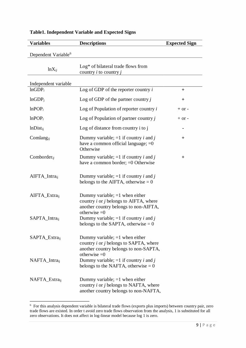
Table1. Independent Variable and Expected Signs

Variables Descriptions Expected Sign

Dependent Variable6

lnXij Log* of bilateral trade flows from

country i to country j

Independent variable

lnGDPi Log of GDP of the reporter country i +

lnGDPj Log of GDP of the partner country j +

lnPOPi Log of Population of reporter country i + or -

lnPOPi Log of Population of partner country j + or -

lnDistij Log of distance from country i to j -

Comlangij Dummy variable; =1 if country i and j

have a common official language; =0

Otherwise

+

Comborderij Dummy variable; =1 if country i and j

have a common border; =0 Otherwise +

AIFTA_Intraij Dummy variable; =1 if country i and j

belongs to the AIFTA, otherwise = 0

AIFTA_Extraij Dummy variable; =1 when either

country i or j belongs to AIFTA, where

another country belongs to non-AIFTA,

otherwise =0

SAPTA_Intraij Dummy variable; =1 if country i and j

belongs to the SAPTA, otherwise = 0

SAPTA_Extraij Dummy variable; =1 when either

country i or j belongs to SAPTA, where

another country belongs to non-SAPTA,

otherwise =0

NAFTA_Intraij Dummy variable; =1 if country i and j

belongs to the NAFTA, otherwise = 0

NAFTA_Extraij Dummy variable; =1 when either

country i or j belongs to NAFTA, where

another country belongs to non-NAFTA,

6 For this analysis dependent variable is bilateral trade flows (exports plus imports) between country pair, zero

trade flows are existed. In order t avoid zero trade flows observation from the analysis, 1 is substituted for all

zero observations. It does not affect in log-linear model because log 1 is zero.

10 | P a g e

otherwise =0

MERCOSURE_Intraij Dummy variable; =1 if country i and j

belongs to the MERCOSURE, otherwise

= 0

MERCOSURE_Extraij Dummy variable; =1 when either

country i or j belongs to MERCOSURE,

where another country belongs to non-

MERCOSURE, otherwise =0

EU15_Intarij Dummy variable; =1 if country i and j

belongs to the EU15, otherwise = 0

EU15_Extraij Dummy variable; =1 when either

country i or j belongs to EU15, where

another country belongs to non-EU15,

otherwise =0

*Natural Log.

There are two way of measuring economic size of country in the gravity model: GDP or

population. The high level of income (GDP) in reporting country (i) indicates a high level

of production which increases the availability of goods for trade. Therefore we expect the

coefficient sign of reporter country’s GDPi to be positive. The coefficient sign of partner

country’s GDPj is also positive because a high level of income (GDP) in the partner country

indicates higher purchasing power of goods.

The estimated coefficient sign of population of the reporting country may be positive or

negative (Oguledo and Macphee 1994) depending on weather a big country trades more than

a small country (economies of scale effect) or weather the country trades less when it is big

(absorption effect), (Martinez & Lehmann 2001). Another factor will also influence the

estimated coefficient sign of population in gravity equation is that the composition effect of

population which influence supply and demand of goods or the mix of goods demanded is

also different for each country. The estimated coefficient sign on population of the partner

country may be positive or negative for similar reasons.

The estimated coefficient sign of distance variable is expected to be negative since it is a

proxy of all possible resistance factors to trade. The geographical proximity of any country

will have positive influence on trade flows between countries. Geographical proximity is

captured through common border dummy variable. Countries having common border will

11 | P a g e

trade more than distance. It will reduce the transaction cost of trade between them. Moreover,

the coefficient of common border variable is expected to be positive. Since the basic gravity

model is log-linear form, the coefficient of dummy variable is interpreted by taking its

exponent (Frankel, 1997). For instance, if the value of common border coefficient is 0.60, it

indicates that two countries having a common border trade 82 [exp (0.60)-1*100] per cent

more trade than those without having common border.

Another essential factor is affecting trade flows are cultural link among countries. The

presence of common language will indicate the cultural familiarity between members; hence

the cultural link will reduce the transaction cost among countries. The cultural link is

captured through official common language dummy variable. The estimated coefficient of

common language variable is also expected to be positive.

Finally, we have incorporated FTAs dummies to estimate agricultural trade creation or

diversion effects of the AIFTA, SAPTA, NAFTA, MERCOSURE and EU15. First, dummy

variables are constructed to measure agricultural intra trade enhancing effect (TC) of FTAs

on the members. These dummies are, AIFTA_Intraij, SAPTA_Intraij, NAFTA_Intraij,

MERCOSURE_Intraij and EU15_Intraij. After the formation of FTAs members will expand

their trade among members through eliminating tariff and non-tariff barriers. Hence, a

positive value implies that the FTAs have contributed to increased trade among its member

countries (TC effect). Secondly, we incorporated another dummies to measure agricultural

trade diversion effect of FTAs on non-members. These dummies are, AIFTA_Extraij,

SAPTA_Extraij, NAFTA_Extraij, MERCOSURE_Extraij and EU15_Extraij. The formation of

FTAs members will increase trade among them while simultaneously reducing trade with

non-members. Hence, a negative values it implies that trade diversion effects of FTAs,

whereas positive value suggest that absence of diversion effects on non-members.

Data Source

The sample size uses fifty countries of Asia, European Union, United States and South

American continents that part of five regional trade agreement (SAPTA, AIFTA, NAFTA,

MERCOSURE and EU). These countries are selected on the basis of export and import share

of major Asian- India Free Trade Agreement (AIFTA) members. The major AIFTA members

are Cambodia, India, Indonesia, Malaysia, Philippines, Singapore, Thailand and Vietnam.

These eight are selected for the analysis and the other three countries namely, Brunei, Laos

PDR and Myanmar are excluded due to non-availability of data.

12 | P a g e

The study cover ten years of data from 2005 to 2014 i.e. five years pre and five years post-

AIFTA analysis. AIFTA come into force in the year of 2010. The total number of

observations are 24500 [50*49*10] for ten years from 2005 to 2014. It includes six SAPTA

countries, seven ASEAN countries, three NAFTA countries, six MERCOSURE countries and

fifteen EU countries and other thirteen countries.

The definition of agriculture sector for this analysis is based on Uruguay Round of

Agreement on Agriculture (URAoA) and Harmonized Commodity Description and Coding

System (HS)7. Bilateral trade data compiled from World Integrated Trade Solution (WITS)

which sourced from UN Comtrade data base. Gross Domestic Products (GDP), Per Capita

GDP and Population data were obtained from the World Development Indicators database.

Bilateral trade flows and GDP are at current prices. Earlier studies found that there is only

marginal difference exist while using real prices. For instance, Srinivasan (1995) showed that

purchasing power parity rates are subject to large measurement error. Frankel (1997) found

little difference in the gravity equation results using real data. Data on common language,

common border and distance taken from Centre d’Etudes Prospective et d’Informations

Internationals.8 CEPII uses the great circle formula to calculate the geographic distance

between countries, referenced by latitudes and longitudes of the largest urban agglomerations

in terms of population.

Estimation Result

The following result estimated using equation 3 with various fixed dummy variable to control

endogeneity. Table 2 include the result listed columns 1 to 3. For equation 3 used random

effect model (GLS), which includes zero trade flows observation with adding small fraction.

First column gives result with time fixed but no country fixed effect, second column with

time, reporter and partner country fixed effect, and third column is with time and country pair

fixed effect.

7 It follows HS code 01 to 24 (excluding fish and fish products). It also include HS code 2905.43(mannitol), HS

Code 2905.44(sorbitol), HS Code 33.01(essential oils), HS code 35.01 to 35.05(albuminoidal substances,

modified starches, glues), HS Code 3809.10(finishing agents), HS Code 3823.06(sorbitol n.e.p.), HS Code 41.01

to 41.03(hides & skins), HS Code 43.01(raw fur skins), HS Code 50.01 to 50.03(raw silk & silk waste), HS Code

51.01 to 51.03(wool & animal hair) HS Code 52.01 to 52.03(raw cotton, waste and cotton carded or combed),

HS Code 53.01(raw flax) and HS Code53.02(raw hemp).

8 http://www.cepii.fr/CEPII/en/bdd/_modele/download.asp?id=6.

13 | P a g e

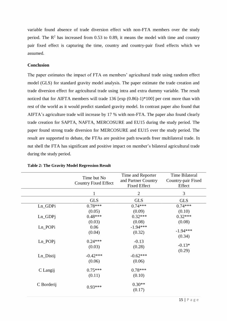
Impact of GDP, Population, Distance and Language

The model with time fixed effect shows the estimated GDP coefficient for both reporter and

partner country have the expected positive sign. The magnitude of GDP coefficient for

reporter is greater than partner country. They are significant at the 1 % level of significance.

Hence, results indicated that there is positive relationship between country pair income and

bilateral trade. The estimated coefficient of population for reporter country was shows

statistical insignificant sign. Contrast, the magnitude of partner country population coefficient

was notice statistical significant at 1 per cent level. It implies that estimated coefficient of

population in partner countries will have greater impact on bilateral trade between pair. The

bilateral variables such as distance, common language and common border have expected

sign and statistical significance. Among bilateral variable the magnitude of common border

(0.93) is higher than other variables. It shows that courtiers having common border will trade

more than distance. The result are support the ‘natural’ trading hypotheses.

The model with time, reporter and partner country fixed effect shows similar sing for GDP

coefficient as it was in time fixed effect model. But, the magnitude of GDP coefficient has

declined for both reporter and partner country. It means country specific fixed such as

infrastructure, level of development etc. affecting bilateral trade between pair. The estimated

coefficient of population for reporter has turns from statistical insignificant to significant

level. Contrast, for partner country has turns from statistical significant to insignificant level.

The other bilateral variables are similar to the previous one but the magnitude has change.

For instance the estimated value of common border has declined for 0.93 to 0.30.

The model with time and country pair fixed effect listed in column 3 shows the similar sign

for GDP and population coefficient as previous one except partner country. The distance,

common language and common border (time invariant variable) capture the country pair

fixed effect dummy variable. The time invariant variable fall out of the model because the

country-pair fixed effects encompass them (Lin & Reed, 2010)

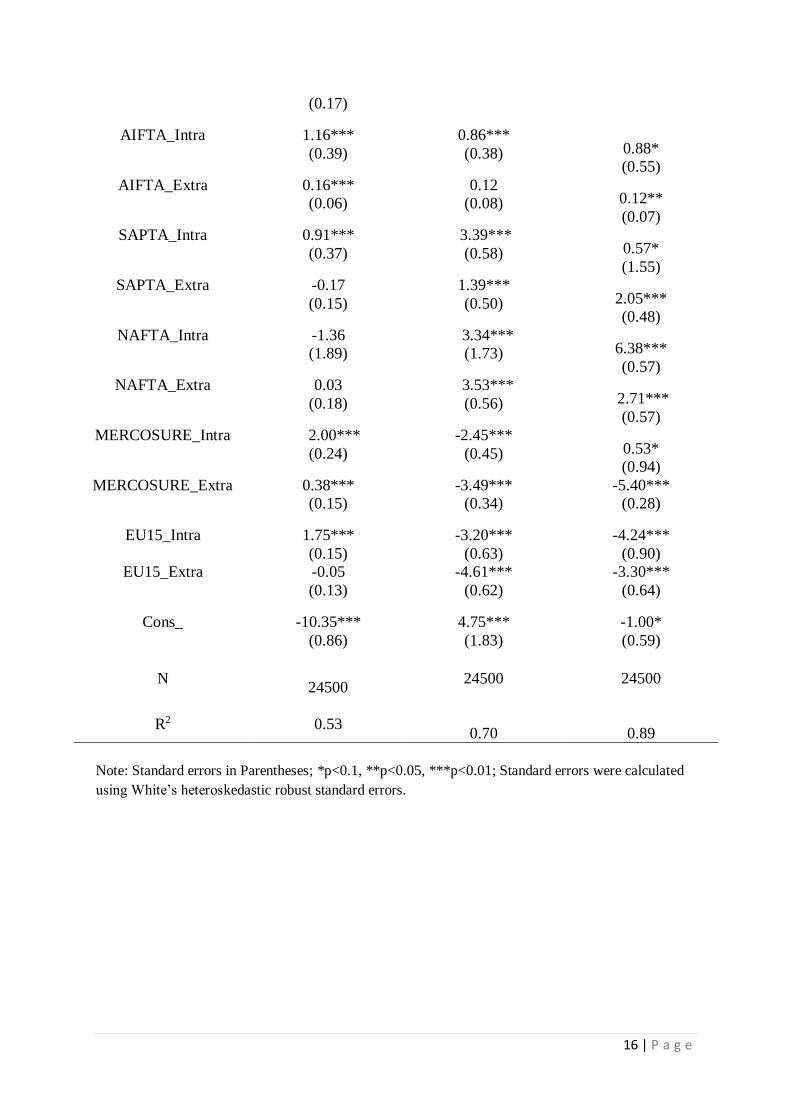
Impact of Intra FTAs Dummy Variable (TC)

The model with only time fixed effects shows the trade creation effects for ASIAN-India free

trade Agreement (AIFTA), South Asian Preferential Trade Agreement (SAPTA), Southern

Common Market (MERCOSURE) and European Union (EU) 15. The result indicates that

intraregional agricultural trade among AIFTA members increase by 219 % [exp (1.16)-

14 | P a g e

1)*100] more than they traded with rest of the world. For SAPTA, MERCOSURE and EU15

shows purely trade creation for agricultural trade among members. The estimated coefficient

of NAFTA dummy was found statistical insignificant.

The model with time, reporter and partner country fixed effect shows that significant trade

creation effect for AIFTA, SAPTA and NAFTA among them. The magnitude of the SAPTA

and NAFTA is found more than AIFTA. For NAFTA, it found statistical insignificant in the

previous model, but it turns at statistical significant level at 1 %. It showing a stronger

magnitude compare to other coefficient. For MERCOSURE and EU15 it turns negative,

showing absence of trade creation among them. Finally, the result suggest that for AIFTA

members will trade 136 [exp(0.86)-1)*100] per cent more than with rest of the world as it

would predict standard gravity model.

The model with time and country pair fixed effect listed in column 3 shows that trade

creation effects among members except EU15. The magnitude of NAFTA variable found

more than any other FTAs dummy variable. For the AIFTA and SAPTA which are found to

increase intraregional trade among members by 141 per cent and 76.82 per cent respectively.

For NAFTA result found more ambiguous. Overall the formation of FTA agriculture trade

has increased among members, it shows that formation of FTA it will positively affect on

agricultural trade among them.

Impact of Extra FTAs Dummy Variable (TD)

The model with only time fixed effects shows that for AIFTA and MERCOSURE found

statistical significant and all other found statistical insignificant. The result is indicating that

after the formation of FTA agriculture trade has increased with non-FTA members. For

instance, AFITA and MERCOSURE agriculture trade will increase by 17 % and 46 % with

non-FTA respectively.

The model with time, reporter and partner country fixed effect for MERCOSURE and EU15

found negative sign for extra dummy variable. It shows purely trade diversion effect with

respect to non-FTA members during the study period. For SAPTA and NAFTA found

absence of trade diversion effect.

Finally the model with time and country pair fixed effect listed in column 3 shows that that

purely trade diversion effects for the MERCOSURE and EU during the study period but these

result are not supported to the earlier findings of the study. The remaining extra dummy

15 | P a g e

variable found absence of trade diversion effect with non-FTA members over the study

period. The R2 has increased from 0.53 to 0.89, it means the model with time and country

pair fixed effect is capturing the time, country and country-pair fixed effects which we

assumed.

Conclusion

The paper estimates the impact of FTA on members’ agricultural trade using random effect

model (GLS) for standard gravity model analysis. The paper estimate the trade creation and

trade diversion effect for agricultural trade using intra and extra dummy variable. The result

noticed that for AIFTA members will trade 136 [exp (0.86)-1)*100] per cent more than with

rest of the world as it would predict standard gravity model. In contrast paper also found that

AIFTA’s agriculture trade will increase by 17 % with non-FTA. The paper also found clearly

trade creation for SAPTA, NAFTA, MERCOSURE and EU15 during the study period. The

paper found strong trade diversion for MERCOSURE and EU15 over the study period. The

result are supported to debate, the FTAs are positive path towards freer multilateral trade. In

nut shell the FTA has significant and positive impact on member’s bilateral agricultural trade

during the study period.

Table 2: The Gravity Model Regression Result

Time but No

Country Fixed Effect

Time and Reporter

and Partner Country

Fixed Effect

Time Bilateral

Country-pair Fixed

Effect

1 2 3

GLS GLS GLS

Ln_GDPi 0.78***

(0.05)

0.74***

(0.09)

0.74***

(0.10)

Ln_GDPj 0.48***

(0.03)

0.32***

(0.08)

0.32***

(0.08)

Ln_POPi 0.06

(0.04)

-1.94***

(0.32) -1.94***

(0.34)

Ln_POPj 0.24***

(0.03)

-0.13

(0.28) -0.13*

(0.29)

Ln_Distij -0.42***

(0.06)

-0.62***

(0.06)

C Langij 0.75***

(0.11)

0.78***

(0.10)

C Borderij 0.93***

0.30**

(0.17)

16 | P a g e

(0.17)

AIFTA_Intra 1.16***

(0.39)

0.86***

(0.38) 0.88*

(0.55)

AIFTA_Extra 0.16***

(0.06)

0.12

(0.08) 0.12**

(0.07)

SAPTA_Intra 0.91***

(0.37)

3.39***

(0.58) 0.57*

(1.55)

SAPTA_Extra -0.17

(0.15)

1.39***

(0.50) 2.05***

(0.48)

NAFTA_Intra -1.36

(1.89)

3.34***

(1.73) 6.38***

(0.57)

NAFTA_Extra 0.03

(0.18)

3.53***

(0.56) 2.71***

(0.57)

MERCOSURE_Intra 2.00***

(0.24)

-2.45***

(0.45) 0.53*

(0.94)

MERCOSURE_Extra 0.38***

(0.15)

-3.49***

(0.34)

-5.40***

(0.28)

EU15_Intra 1.75***

(0.15)

-3.20***

(0.63)

-4.24***

(0.90)

EU15_Extra -0.05

(0.13)

-4.61***

(0.62)

-3.30***

(0.64)

Cons_ -10.35***

(0.86)

4.75***

(1.83)

-1.00*

(0.59)

N 24500

24500

24500

R2 0.53

0.70

0.89

Note: Standard errors in Parentheses; *p<0.1, **p<0.05, ***p<0.01; Standard errors were calculated

using White’s heteroskedastic robust standard errors.

17 | P a g e

Reference:

Anderson J. E. (1979), A Theoretical Foundation of the Gravity Model. American Economic

Review 69 (1): 106-116.

Anderson, J. E and E. Van Wincoop. (2003), Gravity with Gravitas: A Solution to the Border

Puzzle. American Economic Review 93 (1): 170-192.

Bair, S. L. And Bergstrand, J. H. (2007), Do free Trade Agreement Actually Increase

Members’ International Trade? Journal of International Economics 71 (1):72-95.

Burger, M., Oort, F. And Linders, G. (2009), On the Specification of the Gravity Model of

Trade: Zeros,Excess Zerosand Zero-Inflated Estimation. Spatial Economic Analysis

4(2): 167-190.

Bhagwati, J and Krueger A. O.ed. (1995),The Dangerous Drift to Preferential Trade

Agreements. Washington DC, American Enterprise, Institute for Public Policy

Research.

Brun et. al. (2005), Has Distance Died? Evidence from a panel gravity Model, The World

Economy Review, 19(1): 99-120.

Carrere, C. (2006), Revisiting the Effects of Regional Trade Agreements on Trade flows with

Proper Specification of the Gravity Model. European Economic Review 50(2): 223-

247.

Deaedorff, A. (1998), Determinants of Bilateral Trade: Does gravity Work in a Classical

World? In: The Regionalization of the world Economy, ed. Jaffery Frankel, Chicago

University Press.

Eichengreen, B. and Irwin D. A. (1998), The Role of History in Bilateral Trade Flows. NBER

Chapters In: The Regionalization of the world Economy, ed. Jaffery Frankel, 33-57.

Chicago University Press.

Endoh M.(1999), Trade creation and Trade Diversion in the EEC, the LAFTA and the

CMEA: 1960-1994. Applied Economics 31(2): 207-216.

Freund, C. (2000), Different Paths to Free Trade: The gains From Regionalism. Quarterly

Journal of Economics 115(4):1317-1341.

Fukao, K, and Okubo, T. (2003), An Econometric Analysis of Trade Diversion under

NAFTA. North American Journal Economics & Finance 14(1): 2-24.

Filippini C, and Molini V. (2003), The determinants of East Asian trade flows: a Gravity

Equation Approach. Journal of Asian Economics 14(5): 695-711.

18 | P a g e

Frankel, J. A. (1997), Regional Trading Blocs in the world Economic System. Washington

DC, Institute for International Economics.

Frankel, J. A. (1998), the Regionalization of the World Economy. Chicago University Press

Ghosh S, and Yamarik S. (2004), Are Regional Trading Arrangements Trade Creating? An

Application of Extreme Bounds Analysis. Journal of International Economics 63(2):

369-395.

Grant, J. H. And Lambert, D. M.(2008), Do Regional trade Agreements Increase Members’

Agriculture Trade. American Journal of Agricultural Economics 90 (3): 765-782.

Helpman, E. And Krugman, P. (1985), Market Structure and Foreign trade: Increasing

Returns, Imperfect Competition, and the International Economy. Cambridge, MA:

MIT Press.

Helpman, E.(1987), Imperfect Competition and International Trade: Evidence From

Fourteen Industrial Countries . Journal of the Japanese and International Economies

1:62-81.

Jayasinghe, S. And Sarker, R. (2008), Effects of Regional Trade Agreements on Trade in

Agrifood Products: Evidence from Gravity Modelling Using Disaggregate Data.

Review of Agricultural Economics 30(1): 61-81.

Kalirajan, K. (2007), Regional Cooperation and Bilateral Trade Flows: An Empirical

Measurement of Resistance. The International Trade Journal 21(2): 85-107.

Lin, S. And Reed, M.R. (2010), Impact of free Trade Agreements on Agriculture Trade

Creation and Trade Diversion. American Journal of Agricultural Economics 92(5):

1351-1363.

Lambert, D. M. And McKoy S. (2009), Trade Creation and Diversion Effects of Preferential

Trade Association on Agricultural and Food Trade. Journal of Agricultural

Economics 60(1): 17-39.

Levy, P.I. (1997), A Political Economy Analysis of Free-Trade Agreements. American

Economic Review 87(4): 506-519.

Lee H, and Park I.(2007), In Search of Optimized Regional Trade Agreements and

Applications to East Asia”. World Economy 30(5): 783-806.

Musila J.(2005), The Intensity of Trade Creation and Trade Diversion in COMESA, ECCAS

and ECOWAS: a Comparative Analysis. Journal of African Economics 14(1): 117-

141.

19 | P a g e

Martinez, I. and Lehmann, L.(2001), Augmented Gravity Model: An Empirical Application

to MERCOSURE-European Union Trade Flows. Journal of Applied Economics 2:

291-316.

Matyas, L. (1997), Proper Econometric Specification of the Gravity Model, The World

Economy 20(3): 363-368.

Oguledo, V. and Macphee, C. (1994), Gravity Models: A Reformulation and an Application

to Discriminatory Trade Agreements. Journal of Applied Economics 26: 107-120.

Peridy N. (2005), Toward a Pan-Arab Free Trade Area: Assessing Trade Potential Effects of

the AGADIR Agreement. Development Economics XLIII-3: 329-345.

Santos S. And Tenreyro, S. (2006), The Log of gravity. Review of Economics and Statistics

88(4):641-658.

Soloago, I. and Winters, A. (2001), How Has Regionalism in the 1990sAffected Trade?

North American Journal of Economics and Finance 12(1):1-29.

Suranovic, S. M. (2010), International Trade: Theory and policy, George Washington

University.

Tang D. (2005), Effects of the Regional Trading Arrangements on Trade: Evidence from the

NAFTA, ANZCER and ASEAN Countries, 1989-2000. The Journal of International

Trade & Economic Development 14(2): 241-265.

Tinbergen, J. (1962), Shaping the World Economy: Suggestions for an International

Economic Policy. New York: The Twentieth Century Fund.

20 | P a g e

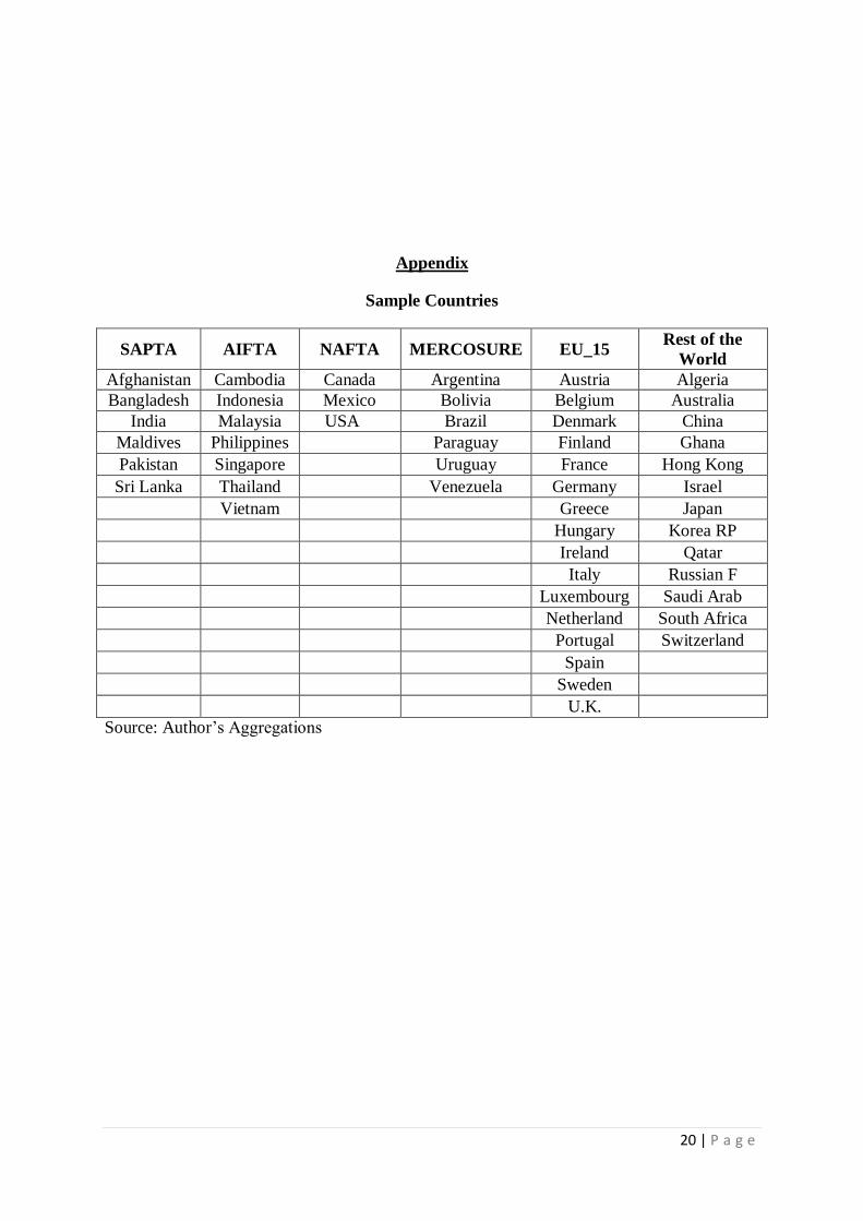
Appendix

Sample Countries

SAPTA AIFTA NAFTA MERCOSURE EU_15 Rest of the

World

Afghanistan Cambodia Canada Argentina Austria Algeria

Bangladesh Indonesia Mexico Bolivia Belgium Australia

India Malaysia USA Brazil Denmark China

Maldives Philippines Paraguay Finland Ghana

Pakistan Singapore Uruguay France Hong Kong

Sri Lanka Thailand Venezuela Germany Israel

Vietnam Greece Japan

Hungary Korea RP

Ireland Qatar

Italy Russian F

Luxembourg Saudi Arab

Netherland South Africa

Portugal Switzerland

Spain Sweden U.K.

Source: Author’s Aggregations