EFFECT OF SLAB SIZE ON AIRPORT PAVEMENT PERFORMANCE · Effects of Slab Size on Airport Pavement...

DOT/FAA/AR-99/83

Office of Aviation Research Washington, D.C. 20591

Effects of Slab Size on Airport Pavement Performance

April 2000

Final Report

This document is available to the U.S. public through the National Technical Information Service (NTIS), Springfield, Virginia 22161.

U.S. Department of Transportation Federal Aviation Administration

NOTICE

This document is disseminated under the sponsorship of the U.S. Department of Transportation in the interest of information exchange. The United States Government assumes no liability for the contents or use thereof. The United States Government does not endorse products or manufacturers. Trade or manufacturer's names appear herein solely because they are considered essential to the objective of this report. This document does not constitute FAA certification policy. Consult your local FAA aircraft certification office as to its use.

This report is available at the Federal Aviation Administration William J. Hughes Technical Center's Full-Text Technical Reports page: www.actlibrary.tc.faa.gov in Adobe Acrobat portable document format (PDF).

Technical Report Documentation Page

1.

DOT/FAA/AR-99/83

2. Government Accession No. 3.

4. itle and Subtitle

EFFECTS OF SLAB SIZE ON AIRPORT PAVEMENT PERFORMANCE

5.

April 2000

6. ing Organization Code

7. uthor(s)

Edward Guo

8. ing Organization Report No.

9. ing Organization Name and Address

Galaxy Scientific Corporation

10. RAIS)

2500 English Creek Ave., Bldg. 11 Egg Harbor Twp., NJ 08234

11.

12. gency Name and Address

U.S. Department of Transportation Federal Aviation Administration

13. ype of Report and Period Covered

Final Report

Office of Aviation Research Washington, DC 20591

14. gency Code

AAS-200 15. entary Notes

Federal Aviation Administration William J. Hughes Technical Center COTR: . Satish Agrawal

16. bstract

The objective of this research is to evaluate the influence of slab size on the performance of rigid pavements by analysis of airport survey data in conjunction with theoretical analysis. he analytical results indicate that when the larger Portland cement concrete (PCC) slabs are used, the maximum total stresses caused by aircraft loading in combination with temperature gradient are significantly greater than those in the smaller slabs. Therefore, cracks would occur in larger slabs earlier since the cracks are mainly controlled by total stress rather than the load-induced stresses. About 288 million square feet (msf) Pavement Condition Index (PCI) data of PCC pavement from 174 airports have been collected from existing pavement databases and survey reports. he PCI has been used to represent the pavement performance. he relationship between slab size and PCI has been investigated by different procedures including the general effect of the slab size on the measured PCI, the effect of slab size influenced by pavement type and age, PCI distribution curves, and special case studies for 14 airports using different slab sizes in the same area. ajor findings are summarized below:

• Slabs larger than 25 by 25 ft performed much more poorly than smaller slabs, which indicates that reinforcement does not have a significantly positive impact on the pavement performance.

• Slabs with 20-foot joint spacing exhibited better performance than slabs with 25-foot joint spacing for all pavement functional areas (runway, taxiway, and apron).

• It is desirable to use smaller slabs, particularly for apron areas.

• Further studies are needed to determine the optimal joint spacing range within 10 to 20 feet for apron pavements.

17. Words

Rigid pavement, Pavement condition, Pavement Condition Index (PCI), Slab size, Temperature gradient

18. ent

This document is available to the public through the National Technical Information Service (NTIS), Springfield, Virginia 22161.

19. Classif. (of this report)

Unclassified

20. Classif. (of this page)

Unclassified

21.

94

22.

N/A

Report No. Recipient's Catalog No.

T Report Date

Perform

A Perform

Perform Work Unit No. (T

Contract or Grant No.

Sponsoring A T

Sponsoring A

Supplem

Dr

A

T

TT

M

Key Distribution Statem

Security Security No. of Pages Price

Form DOT F1700.7 (8-72) Reproduction of completed page authorized

TABLE OF CONTENTS

Page

EXECUTIVE SUMMARY

INTRODUCTION

PART ONE: FINITE ELEMENT ANALYSIS

Analytical Model and Finite Element MeshesResponse Under Different Gear ConfigurationsVariables Affecting Critical Stresses (No Temperature Variation)Analysis With Initial Warping or CurlingEffects of Initial Slab Deformation (Warping and Curling)Analysis Based on Total StressEffects of Joint Load Transfer on the Critical StressesSummary of Findings

PART TWO: STATISTICAL ANALYSIS OF FIELD SURVEYED DATA

IntroductionStatistical Concepts Used in the AnalysisAssumptions Used in the AnalysisGeneral Survey InformationData SelectionVariation of PCI by Pavement Type and AgeGeneral Effects of Slab Size on PCIEffects of Age and Year of ConstructionAnalysis of PCI Distribution CurvesCase Study of Fourteen Airports

CONCLUSIONS

REFERENCES

APPENDIX A−Computational Results

vii

1

3

3 12 13 15 17 22 25 27

29

29 31 32 33 38 41 43 46 50 54

59

61

iii

1

2

3

4

5

6

7

8

9

10

11

12

13

14

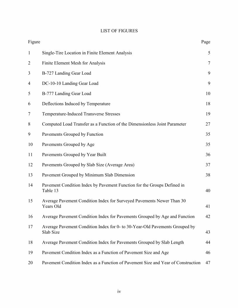
LIST OF FIGURES

Figure Page

Single-Tire Location in Finite Element Analysis

Finite Element Mesh for Analysis

B-727 Landing Gear Load

DC-10-10 Landing Gear Load

B-777 Landing Gear Load

Deflections Induced by Temperature

Temperature-Induced Transverse Stresses

5

7

9

9

10

18

19

Computed Load Transfer as a Function of the Dimensionless Joint Parameter 27

Pavements Grouped by Function 35

Pavements Grouped by Age 35

Pavements Grouped by Year Built 36

Pavements Grouped by Slab Size (Average Area) 37

Pavement Grouped by Minimum Slab Dimension 38

Pavement Condition Index by Pavement Function for the Groups Defined inTable 13 40

15 Average Pavement Condition Index for Surveyed Pavements Newer Than 30 Years Old 41

16 Average Pavement Condition Index for Pavements Grouped by Age and Function 42

17 Average Pavement Condition Index for 0- to 30-Year-Old Pavements Grouped by Slab Size 43

18 Average Pavement Condition Index for Pavements Grouped by Slab Length 44

19 Pavement Condition Index as a Function of Pavement Size and Age 46

20 Pavement Condition Index as a Function of Pavement Size and Year of Construction 47

iv

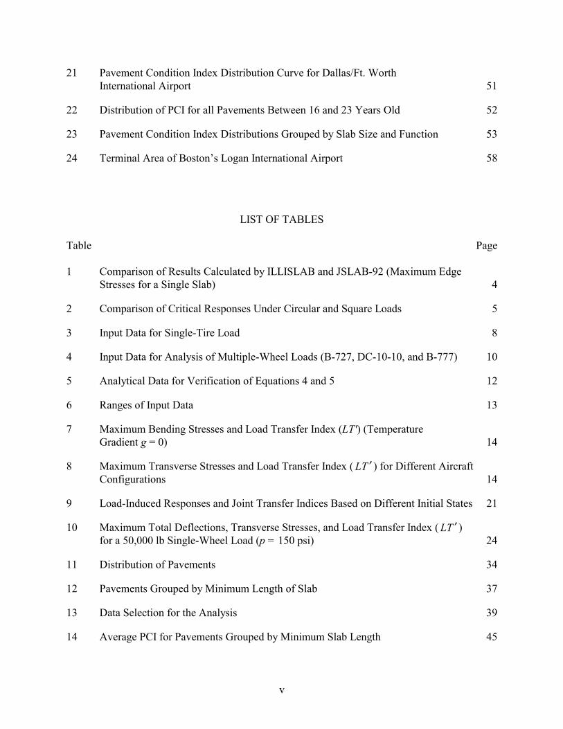
21 Pavement Condition Index Distribution Curve for Dallas/Ft. Worth International Airport 51

22 Distribution of PCI for all Pavements Between 16 and 23 Years Old 52

23 Pavement Condition Index Distributions Grouped by Slab Size and Function 53

24 Terminal Area of Boston’s Logan International Airport 58

LIST OF TABLES

Table Page

1 Comparison of Results Calculated by ILLISLAB and JSLAB-92 (Maximum Edge Stresses for a Single Slab) 4

2 Comparison of Critical Responses Under Circular and Square Loads 5

3 Input Data for Single-Tire Load 8

4 Input Data for Analysis of Multiple-Wheel Loads (B-727, DC-10-10, and B-777) 10

5 Analytical Data for Verification of Equations 4 and 5 12

6 Ranges of Input Data 13

7 Maximum Bending Stresses and Load Transfer Index (LT') (Temperature Gradient g = 0) 14

8 Maximum Transverse Stresses and Load Transfer Index ( LT ′ ) for Different Aircraft Configurations 14

9 Load-Induced Responses and Joint Transfer Indices Based on Different Initial States 21

10 Maximum Total Deflections, Transverse Stresses, and Load Transfer Index ( LT ′ ) for a 50,000 lb Single-Wheel Load (p = 150 psi) 24

11 Distribution of Pavements 34

12 Pavements Grouped by Minimum Length of Slab 37

13 Data Selection for the Analysis 39

14 Average PCI for Pavements Grouped by Minimum Slab Length 45

v

15 Data for Figure 19Pavement Condition Index as a Function of PavementSize and Age 48

16 Data for Figure 20Pavement Condition Index as a Function of PavementSize and Year of Construction 48

17 All Features With Slabs Larger Than 625 sq. ft. 50

18 Apron Pavement Condition Index for Two Slab Size Groups at Eight Airports 55

19 Taxiway Pavement Condition Index for Two Slab Size Groups at Eight Airports 56

20 Runway Pavement Condition Index for Two Slab Size Groups at Three Airports 56

21 Effect of Slab Size on Performance of Pavements in the Same Area 57

22 Pavement Condition Index of Pavements at Boston’s Logan International Airport 57

vi

EXECUTIVE SUMMARY

The objective of this research is to evaluate the influence of slab size on the performance of rigid pavements by analysis of airport survey data in conjunction with theoretical analysis. The analytical results indicate that when larger portland cement concrete (PCC) slabs are used, the maximum total stresses caused by aircraft loading in combination with temperature gradient are significantly greater than those in the smaller slabs. Therefore, cracks are expected to occur earlier in larger slabs, since the cracks are controlled primarily by total stress rather than by the load-induced stresses alone. Pavement Condition Index (PCI) data on approximately 288 million square feet (msf) of PCC pavement from 174 airports were collected from existing pavement databases and survey reports. The PCI is used in this report to represent the pavement performance. This report examines the relationship between slab size and PCI in several different ways, including investigating the effect of the slab size on the measured PCI in general and considering how that effect may be influenced by variables such as pavement type and age; developing PCI distribution curves; and presenting a special case study of 14 airports using different slab sizes for pavements performing similar functions. The major findings are summarized below:

• Slabs larger than 25 by 25 ft performed much more poorly than did smaller slabs, indicating that reinforcement does not have a significantly positive impact on the pavement performance.

• Slabs with 20-foot joint spacing performed better than slabs with 25-foot joint spacing for all airport pavement categories (runway, taxiway, and apron).

• Based on the survey finding that smaller slabs are associated with improved pavement performance for airport apron areas, it is strongly recommended that apron pavements use slab sizes under 500 square feet.

• Further studies are needed to determine the optimal joint spacing for apron pavements within the range of 10 to 20 feet.

vii/viii

INTRODUCTION

For portland cement concrete (PCC) airport pavement construction, the joint spacing and the corresponding slab size are determined during design. Federal Aviation Administration (FAA) Advisory Circular (AC) 150/5320-6D [1] offers the following rule of thumb to determine the slab size based on the Portland Cement Association (PCA) design method [2]: “the joint spacing (in feet) should not greatly exceed twice the slab thickness (in inches)” and “ratio of slab length to slab width should not exceed 1.25 for unreinforced pavements.” Table 3-7 of reference 1 provides the recommended maximum joint spacings for unreinforced pavements. For all pavement slab thicknesses equal to or greater than 12 in., the recommended maximum spacing for transverse and longitudinal joints is 25 ft (7.6 m). Since almost all major airports that serve heavy jet aircraft require a slab thickness greater than 12 in., 25 by 25 ft has been the most common slab size currently used at large- and medium-hub airports.

The PCA design method states that 20 to 25 ft longitudinal construction joint spacing was used (before 1973) because the “equipment was best suited to paving widths of 20 to 25 ft” [2]. However, since the 1970s, developments in paving equipment have permitted construction widths up to 50 ft, and the question arises of whether the standard 25- by 25-ft size should still be followed to build and rehabilitate unreinforced airport PCC pavements. From a practical point of view, some airport pavement engineers have found that pavements with a slab size larger than 25 ft usually crack earlier than pavements using smaller slabs, such as 12.5 by 12.5 ft. Smaller slabs have also been recognized as offering better performance by engineers in other countries, such as India [3], who suggest using 13- to 16.4-ft size slabs in hot weather.

For reinforced concrete pavements, both the FAA and PCA design methods allow the use of larger joint spacing. AC 150/5320-6D allows contraction joint spacing of up to 75 ft. The PCA method [2] suggests using joint spacings ranging from 30 to 70 ft, depending on slab thickness. Both methods require the use of dowels for the reinforced concrete pavement joints to avoid a loss of load transfer capability due to larger joint openings in the regions with wide temperature variations between summer and winter.

Using larger slabs has advantages and disadvantages. The advantages of using large slabs are:

• reduction in the number of joints and thus reduction of the cost of pavements.

• reduction in the cost of joint maintenance, since all expansion and construction joints need routine resealing.

• smoother surface condition.

The disadvantages of using large slabs are:

• possibility of earlier cracks in the slabs (this has been observed by airport engineers).

• larger slab movement and joint opening, which reduces the joint load transfer capability.

• critical responses larger than those in smaller slabs.

1

Theoretical and numerical analyses on the slab size effects on pavement responses have been conducted by some investigators. The results of reference 4 indicate that temperature-induced pavement responses are very important in comparison to load-induced responses and should not be neglected. Reference 5 developed a warping stress equation based on a stress analysis using the finite element method. Reference 6 calculated the temperature-induced responses using a nonlinear model to simulate the temperature variation along the slab thickness.

The objective of this research is to evaluate the influence of slab size on the performance of rigid pavements by analysis of airport survey data in conjunction with theoretical analysis. The analytical results are presented in part one and the statistical results of surveyed data are given in part two.

The following effects have been considered in the theoretical analysis:

• The effects of the slab size on the load-induced critical stress of the slab under different aircraft gears without considering the temperature variation.

• The effects of the slab size on the load-induced critical stress of the slab under different aircraft gears considering the temperature variation.

• The effects of the slab size on the joint load transfer capability.

• The effects of the slab size on the critical stress and joint load transfer capability based on total stresses caused by temperature differences at the top and bottom of the slabs and the loading.

• The effects of joint load transfer on the critical responses in PCC pavement.

The theoretical analysis is not sufficient to find the optimal slab size for airport pavement design or rehabilitation because performance of the pavement cannot be directly predicted by the calculated critical response in the slabs. Environmental effects on pavement performance cannot be perfectly simulated solely by the temperature variation model employed in the analysis. The performance of the pavement is influenced by many factors which are more complicated than the ones considered in any of the available simplified models. The effects of combining these factors cannot be predicted by any available theoretical model. Airport survey data, including the experience of pavement engineers working at airports, were used to verify the results obtained from theoretical analysis and to find the appropriate slab size.

It is common in pavement surveys to find that in some cases pavements using smaller slabs perform better than those using larger slabs while in other cases the pavements using larger slabs perform better. One of the most important objectives in this project is to separate the effect of slab size from other effects to evaluate the effect of slab size on pavement performance under realistic conditions at airports throughout the United States.

The slab size effect was evaluated by statistical analyses of 288 million square feet of PCC pavement data from 174 airports distributed in six FAA regions, plus Hawaii and Japan. The

2

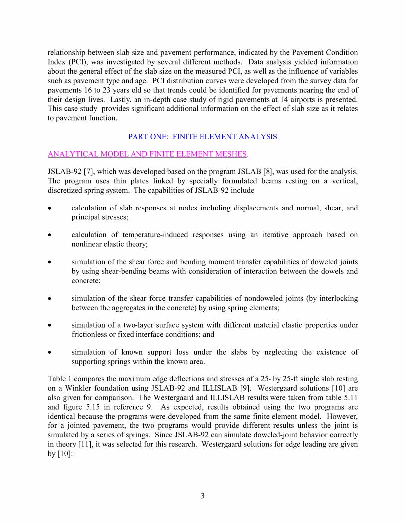
relationship between slab size and pavement performance, indicated by the Pavement Condition Index (PCI), was investigated by several different methods. Data analysis yielded information about the general effect of the slab size on the measured PCI, as well as the influence of variables such as pavement type and age. PCI distribution curves were developed from the survey data for pavements 16 to 23 years old so that trends could be identified for pavements nearing the end of their design lives. Lastly, an in-depth case study of rigid pavements at 14 airports is presented. This case study provides significant additional information on the effect of slab size as it relates to pavement function.

PART ONE: FINITE ELEMENT ANALYSIS

ANALYTICAL MODEL AND FINITE ELEMENT MESHES.

JSLAB-92 [7], which was developed based on the program JSLAB [8], was used for the analysis. The program uses thin plates linked by specially formulated beams resting on a vertical, discretized spring system. The capabilities of JSLAB-92 include

• calculation of slab responses at nodes including displacements and normal, shear, and principal stresses;

• calculation of temperature-induced responses using an iterative approach based on nonlinear elastic theory;

• simulation of the shear force and bending moment transfer capabilities of doweled joints by using shear-bending beams with consideration of interaction between the dowels and concrete;

• simulation of the shear force transfer capabilities of nondoweled joints (by interlocking between the aggregates in the concrete) by using spring elements;

• simulation of a two-layer surface system with different material elastic properties under frictionless or fixed interface conditions; and

• simulation of known support loss under the slabs by neglecting the existence of supporting springs within the known area.

Table 1 compares the maximum edge deflections and stresses of a 25- by 25-ft single slab resting on a Winkler foundation using JSLAB-92 and ILLISLAB [9]. Westergaard solutions [10] are also given for comparison. The Westergaard and ILLISLAB results were taken from table 5.11 and figure 5.15 in reference 9. As expected, results obtained using the two programs are identical because the programs were developed from the same finite element model. However, for a jointed pavement, the two programs would provide different results unless the joint is simulated by a series of springs. Since JSLAB-92 can simulate doweled-joint behavior correctly in theory [11], it was selected for this research. Westergaard solutions for edge loading are given by [10]:

3

δ = P 2 + 1.2µ r

E 1 − (0.76 + 0.4µ) (1) Eh3 k l

r lnσ E =

3(1 + µ )P Eh3 + 1.84 −

4 µ + 1 − µ + 1.18(1 + 2µ) (2)

π (3 + µ )h2 100kr 4

3 2 l

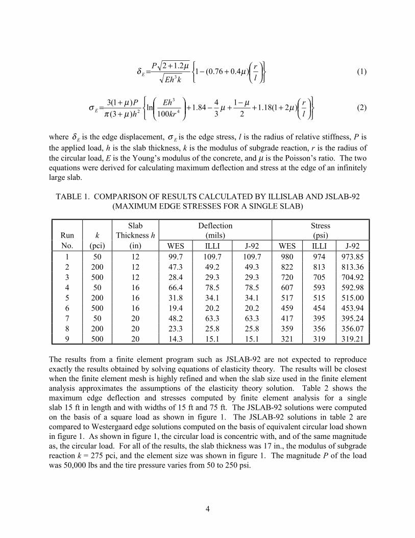
where δ E is the edge displacement, σ E is the edge stress, l is the radius of relative stiffness, P is the applied load, h is the slab thickness, k is the modulus of subgrade reaction, r is the radius of the circular load, E is the Young’s modulus of the concrete, and µ is the Poisson’s ratio. The two equations were derived for calculating maximum deflection and stress at the edge of an infinitely large slab.

TABLE 1. COMPARISON OF RESULTS CALCULATED BY ILLISLAB AND JSLAB-92 (MAXIMUM EDGE STRESSES FOR A SINGLE SLAB)

Run No.

k (pci)

Slab Thickness h

(in)

Deflection (mils)

Stress (psi)

WES ILLI J-92 WES ILLI J-92 1 2 3 4 5 6 7 8 9

50 200 500 50 200 500 50 200 500

12 12 12 16 16 16 20 20 20

99.7 47.3 28.4 66.4 31.8 19.4 48.2 23.3 14.3

109.7 49.2 29.3 78.5 34.1 20.2 63.3 25.8 15.1

109.7 49.3 29.3 78.5 34.1 20.2 63.3 25.8 15.1

980 822 720 607 517 459 417 359 321

974 813 705 593 515 454 395 356 319

973.85 813.36 704.92 592.98 515.00 453.94 395.24 356.07 319.21

The results from a finite element program such as JSLAB-92 are not expected to reproduce exactly the results obtained by solving equations of elasticity theory. The results will be closest when the finite element mesh is highly refined and when the slab size used in the finite element analysis approximates the assumptions of the elasticity theory solution. Table 2 shows the maximum edge deflection and stresses computed by finite element analysis for a single slab 15 ft in length and with widths of 15 ft and 75 ft. The JSLAB-92 solutions were computed on the basis of a square load as shown in figure 1. The JSLAB-92 solutions in table 2 are compared to Westergaard edge solutions computed on the basis of equivalent circular load shown in figure 1. As shown in figure 1, the circular load is concentric with, and of the same magnitude as, the circular load. For all of the results, the slab thickness was 17 in., the modulus of subgrade reaction k = 275 pci, and the element size was shown in figure 1. The magnitude P of the load was 50,000 lbs and the tire pressure varies from 50 to 250 psi.

4

TABLE 2. COMPARISON OF CRITICAL RESPONSES UNDER CIRCULARAND SQUARE LOADS

Tire Pres-

sure, p (psi)

Maximum Deflections (in) Maximum Stresses (psi) JSLAB-92a

Westergaardb

JSLAB-92a

Westergaardb Slab Width

= 15 ft Slab Width

= 75 ft Slab Width

= 15 ft Slab Width

= 75 ft

50 0.0231 0.0277 0.0224 278.5 261.3 270.6 100 0.0254 0.0305 0.0251 362.2 343.6 345.7 150 0.0265 0.0318 0.0264 413.7 394.3 391.2 200 0.0272 0.0326 0.0271 450.3 430.5 423.7 250 0.0276 0.0331 0.0276 478.5 458.4 449.2

aSquare Load, side length: 2a = P p bCircular Load, diameter: 2r = 2 P pπ

2a

2r 1

0 e

lem

ents

@ 1

5 in

ches

30

in

d2 6 elements @ 15 d2 inches

FIGURE 1. SINGLE-TIRE LOCATION IN FINITE ELEMENT ANALYSIS

Table 2 shows that the finite element analyses predict larger edge deflections than Westergaard’s analysis for the smaller slab size (15 ft). However, the maximum edge stresses for the smaller slab are generally closer to the Westergaard solution (which is based on the assumption of an

5

infinitely large slab width). Many numerical examples in reference 9 also show that it is unrealistic to expect that the deflections and stresses calculated by using finite element methods would be identical to those calculated using elastic theory. Both predict identical results in a few special cases. However, prediction of identical results cannot be generalized for all cases appearing in engineering practice. To simulate properly the different features of airport pavements, such as joints and finite-sized slabs, the finite element method was selected as the principal tool to conduct numerical analysis in this project.

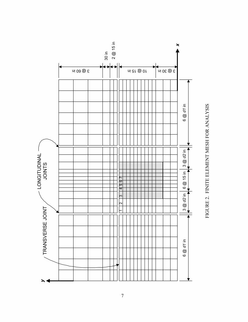
The mesh used in the analysis is shown in figure 2 and contains six slabs linked by one transverse joint and two longitudinal joints. Slab length was held constant at 20 ft because the length has an insignificant effect on the critical stress when the gear load is located either at the edge of the transverse joint or at the corner of one slab. The width of the slabs was varied from 15 ft (Group 1), 20 ft (Group 2), and 25 ft (Group 3) to investigate the effect of slab width. The widths of d1 and d2 varied corresponding to the slab width used in analysis. For example, d1 = 40 in. and d2 = 25 in. for the slab width = 20 ft. The relative stiffness (l) is calculated by equation 3:

l = Eh

k −

3

4

12 1 ( µ )(3)

where E is the elasticity modulus of concrete, h is the slab thickness, µ is the Poisson’s ratio of concrete, and k is the subgrade modulus. Thirty-three numerical calculations were performed for the single-tire load using JSLAB-92. The major input data are listed in table 3.

6

TR

AN

SV

ER

SE

JO

INT

L

ON

GIT

UD

INA

L

JOIN

TS

30

in

2 @

15

in

1

2

3

4 5

67

6 @

d1

in

3 @ 30 in 10 @ 15 in

y

6 @

d1

in

3 @

d2

in

6 @

15

in

3 @

d2

in

3 @ 60 in

FIG

UR

E 2

. F

INIT

E E

LE

ME

NT

ME

SH

FO

R A

NA

LY

SIS

7

x

TABLE 3. INPUT DATA FOR SINGLE-TIRE LOAD (See Figure 1)*

Group (Width) ID

Subgrade Modulus k

(pci)

Slab Thickness

h (in)

Radius of Relative

Stiffness l (in)

Temperature Gradient (°F/in)

r/l (Fig. 1)

1 (15 ft)

AT1 AT2 AA1 AA2 AA3 AC1 AC2 AC3 AE1 AE2 AE3

275 275 275 275 275 275 275 275 275 275 275

17 17 17 17 17 17 17 17 17 17 17

50 50 50 50 50 50 50 50 50 50 50

-1.5 1.5 0

-1.5 1.5 0

-1.5 1.5 0

-1.5 1.5

N/A N/A 0.357 0.357 0.357 0.206 0.206 0.206 0.160 0.160 0.160

2 (20 ft)

BT1 BT2 BA1 BA2 BA3 BC1 BC2 BC3 BE1 BE2 BE3

50 50 50 50 50 50 50 50 50 50 50

19 19 19 19 19 19 19 19 19 19 19

82 82 82 82 82 82 82 82 82 82 82

-1.5 1.5 0

-1.5 1.5 0

-1.5 1.5 0

-1.5 1.5

N/A N/A 0.218 0.218 0.218 0.126 0.126 0.126 0.097 0.097 0.097

3 (25 ft)

CT1 CT2 CA1 CA2 CA3 CC1 CC2 CC3 CE1 CE2 CE3

500 500 500 500 500 500 500 500 500 500 500

15 15 15 15 15 15 15 15 15 15 15

39 39 39 39 39 39 39 39 39 39 39

-1.5 1.5 0

-1.5 1.5 0

-1.5 1.5 0

-1.5 1.5

N/A N/A 0.457 0.457 0.457 0.264 0.264 0.264 0.205 0.205 0.205

*Other data used are: E = 4,000,000 psi, µ = 0.15, AGG (spring constant) = 100,000 psi

The following aircraft types were used to investigate the effects of slab size on critical responses: the B-727 (maximum aircraft gross weight 200,000 lbs), the DC-10-10 (gross weight

8

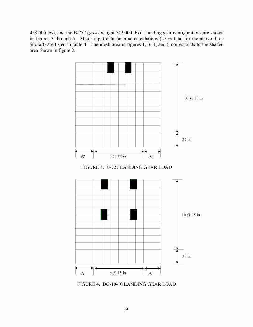
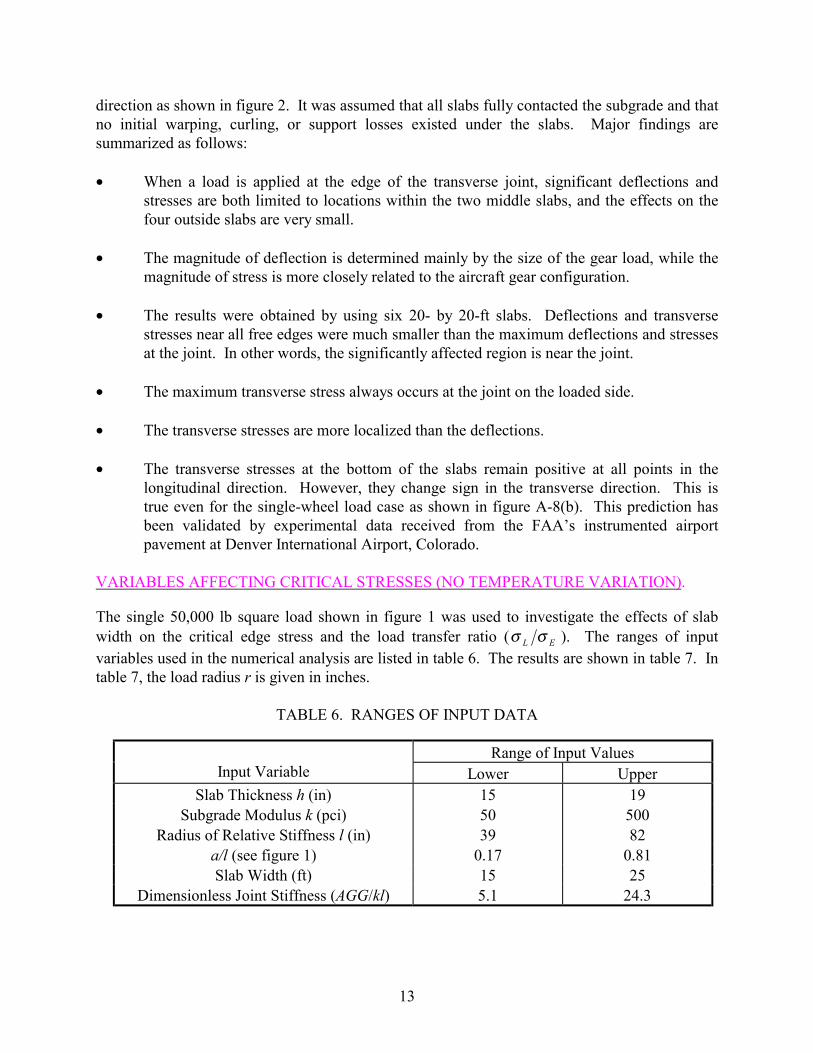
458,000 lbs), and the B-777 (gross weight 722,000 lbs). Landing gear configurations are shown in figures 3 through 5. Major input data for nine calculations (27 in total for the above three aircraft) are listed in table 4. The mesh area in figures 1, 3, 4, and 5 corresponds to the shaded area shown in figure 2.

10 @ 15 in

30 in

d2 6 @ 15 in d2

FIGURE 3. B-727 LANDING GEAR LOAD

10 @ 15 in

30 in

6 @ 15 in d1d1

FIGURE 4. DC-10-10 LANDING GEAR LOAD

9

10 @ 15 in

30 in

d1 6 @ 15 in d1

FIGURE 5. B-777 LANDING GEAR LOAD

TABLE 4. INPUT DATA FOR ANALYSIS OF MULTIPLE-WHEEL LOADS (B-727, DC-10-10, AND B-777)*

Case ID

Slab Width (ft) k (pci)

Slab Thickness h (in)

Relative Stiffness, l (in)

A1 A2 A3 B1 B2 B3 C1 C2 C3

15 20 25 15 20 25 15 20 25

500 500 500 275 275 275 50 50 50

15 15 15 17 17 17 19 19 19

39 39 39 50 50 50 82 82 82

*Dowel bar input values are as follows: dowel bar diameter: D = 1.50 in. (transverse joints)

D = 1.25 in. (longitudinal joints) dowel spacing: s = 18 in joint opening: ω = 0.5 in dowel interaction coefficient: K = 1,500,000 pci

Joint behavior may be modeled simply by a series of springs representing the interlock between aggregates. Doweled joints may be modeled as shear-bending beams with consideration given to

10

interaction between the dowels and the concrete. Alternatively, the doweled joint can be modeled as an equivalent distributed spring. Following reference 12, the equivalent spring constant is designated AGG. Figures 10 and 11 in reference 12 were used to calculate AGG for a doweled joint with known dowel diameter, spacing, material properties, and coefficient of dowel-concrete interaction.

Joint load transfer was analyzed by comparing the critical bending stress in the jointed pavement (σ L ) to the critical bending stress at the free edge (σ E ). For the jointed pavement, the critical stress is the loaded slab along the joint. Equations 4 and 5 are used in reference 12 to derive the load transfer efficiency of the joint.

σ L + σ U = σ E (4)

δ L + δU = δ E (5)

where σ L and δ L are stress and deflection on the loaded side at the pavement joint, σU and δU

are stress and deflection on the unloaded side at the pavement joint, and σ E andδ E are stress and deflection at the free edge of the loaded pavement. The free edge case is equivalent to assuming zero load transfer efficiency for the joint.

Equations 4 and 5 are exact when the joint is simulated by a pure shear load transfer model, and they are approximately true for the shear-bending beam model. The two equations may be applied for various types of gear loads and at all points along the joint. Equations 4 and 5 can also be used to check the accuracy of a finite element program.

Table 5 reports values of σ L , δ L , σU , δU , σ E , and δ E for the DC-10-10 landing gear

(figure 4) calculated by using the JSLAB-92 program. The stresses (σ) are reported in psi and the deflections (δ) are reported in mils. Since the structure in figure 2 and the loading cases are both symmetrical, seven points (1 to 7 in figure 2) are enough to show the distribution of responses on two sides of the transverse joint. The input data are the same as case B2 in table 4. The shear-bending beam models were used to simulate the joint behavior using the dowel bar data in table 4.

Major findings from the analyses are summarized as follows:

• Equations 4 and 5 both have been verified by JSLAB-92 results. Equations 4 and 5 were verified for B-727 and B-777 gear loads in addition to the DC-10-10 load.

• The load transfer efficiency of a pavement under a gear load cannot be defined uniquely using the ratio of deflections (δU δ L ) or stresses (σU σ L ) on two sides of the joint,

since these ratios vary with the location of the points along the joint.

11

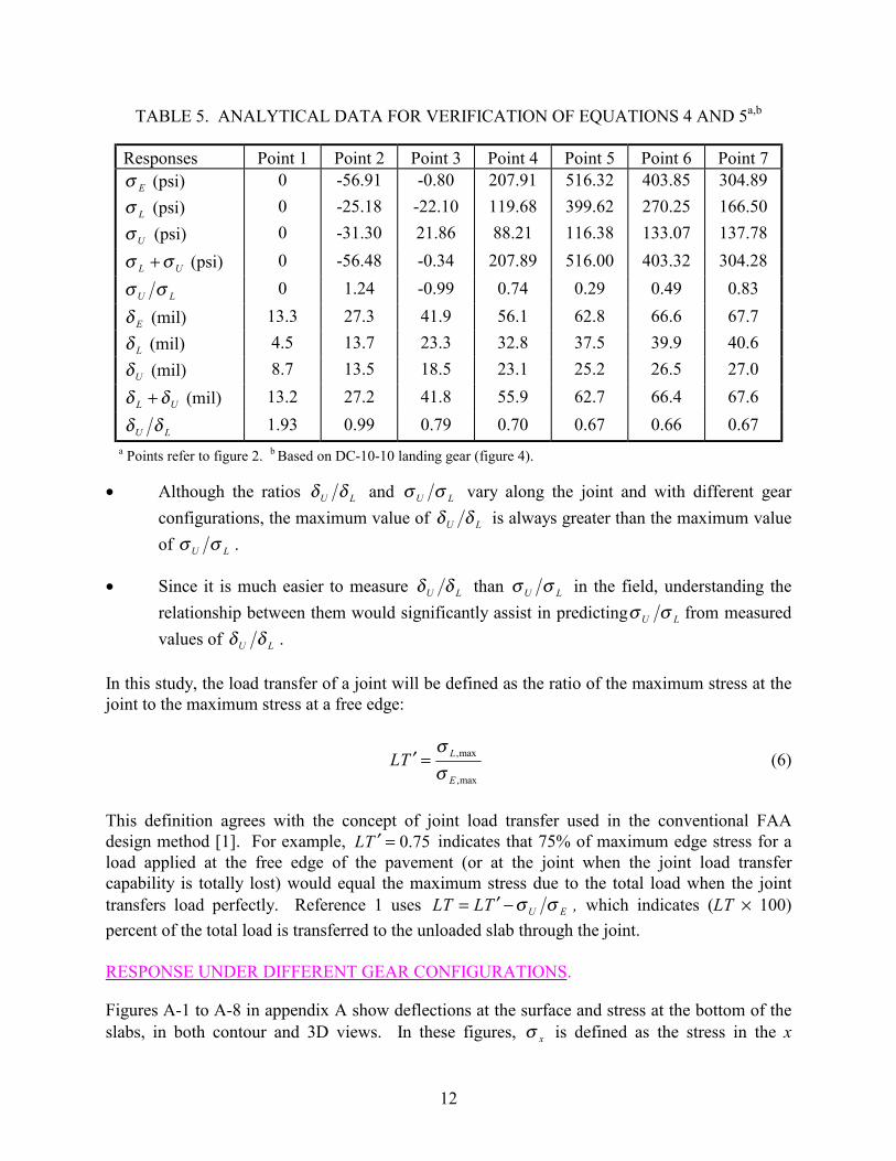
TABLE 5. ANALYTICAL DATA FOR VERIFICATION OF EQUATIONS 4 AND 5a,b

Responses Point 1 Point 2 Point 3 Point 4 Point 5 Point 6 Point 7

Eσ (psi)

Lσ (psi)

Uσ (psi)

UL σσ + (psi)

LU σσ

Eδ (mil)

Lδ (mil)

Uδ (mil)

UL δδ + (mil)

LU δδ

0

0

0

0

0

13.3

4.5

8.7

13.2

1.93

-56.91

-25.18

-31.30

-56.48

1.24

27.3

13.7

13.5

27.2

0.99

-0.80

-22.10

21.86

-0.34

-0.99

41.9

23.3

18.5

41.8

0.79

207.91

119.68

88.21

207.89

0.74

56.1

32.8

23.1

55.9

0.70

516.32

399.62

116.38

516.00

0.29

62.8

37.5

25.2

62.7

0.67

403.85

270.25

133.07

403.32

0.49

66.6

39.9

26.5

66.4

0.66

304.89

166.50

137.78

304.28

0.83

67.7

40.6

27.0

67.6

0.67 a Points refer to figure 2. b Based on DC-10-10 landing gear (figure 4).

• Although the ratios δU δ L and σU σ L vary along the joint and with different gear

configurations, the maximum value of δU δ L is always greater than the maximum value

of σU σ L .

• Since it is much easier to measure δU δ L than σU σ L in the field, understanding the

relationship between them would significantly assist in predictingσU σ L from measured

values of δU δ L .

In this study, the load transfer of a joint will be defined as the ratio of the maximum stress at the joint to the maximum stress at a free edge:

σ LT ′ = L,max (6)

σ E ,max

This definition agrees with the concept of joint load transfer used in the conventional FAA design method [1]. For example, LT ′ = 0.75 indicates that 75% of maximum edge stress for a load applied at the free edge of the pavement (or at the joint when the joint load transfer capability is totally lost) would equal the maximum stress due to the total load when the joint transfers load perfectly. Reference 1 uses LT = LT ′ −σU σ E , which indicates (LT × 100)

percent of the total load is transferred to the unloaded slab through the joint.

RESPONSE UNDER DIFFERENT GEAR CONFIGURATIONS.

Figures A-1 to A-8 in appendix A show deflections at the surface and stress at the bottom of the slabs, in both contour and 3D views. In these figures, σ x is defined as the stress in the x

12

direction as shown in figure 2. It was assumed that all slabs fully contacted the subgrade and that no initial warping, curling, or support losses existed under the slabs. Major findings are summarized as follows:

• When a load is applied at the edge of the transverse joint, significant deflections and stresses are both limited to locations within the two middle slabs, and the effects on the four outside slabs are very small.

• The magnitude of deflection is determined mainly by the size of the gear load, while the magnitude of stress is more closely related to the aircraft gear configuration.

• The results were obtained by using six 20- by 20-ft slabs. Deflections and transverse stresses near all free edges were much smaller than the maximum deflections and stresses at the joint. In other words, the significantly affected region is near the joint.

• The maximum transverse stress always occurs at the joint on the loaded side.

• The transverse stresses are more localized than the deflections.

• The transverse stresses at the bottom of the slabs remain positive at all points in the longitudinal direction. However, they change sign in the transverse direction. This is true even for the single-wheel load case as shown in figure A-8(b). This prediction has been validated by experimental data received from the FAA’s instrumented airport pavement at Denver International Airport, Colorado.

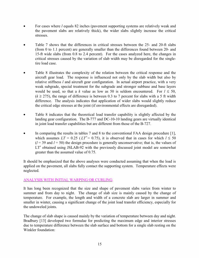
VARIABLES AFFECTING CRITICAL STRESSES (NO TEMPERATURE VARIATION).

The single 50,000 lb square load shown in figure 1 was used to investigate the effects of slab width on the critical edge stress and the load transfer ratio (σ L σ E ). The ranges of input variables used in the numerical analysis are listed in table 6. The results are shown in table 7. In table 7, the load radius r is given in inches.

TABLE 6. RANGES OF INPUT DATA

Input Variable Range of Input Values

Lower Upper Slab Thickness h (in)

Subgrade Modulus k (pci) Radius of Relative Stiffness l (in)

a/l (see figure 1) Slab Width (ft)

Dimensionless Joint Stiffness (AGG/kl)

15 50 39

0.17 15 5.1

19 500 82

0.81 25

24.3

13

TABLE 7. MAXIMUM BENDING STRESSES AND LOAD TRANSFER INDEX (LT') (TEMPERATURE GRADIENT g = 0)

Slab Width = 15 ft max,xσ (psi) LT'

k, pci l, in AGG/kl r = 7.98 r = 10.3 r = 17.84 r = 7.98 r = 10.3 r = 17.84 500 275 50

39 50 82

5.1 7.3 24.3

429.1 378.3 355.9

355.9 319.6 307.5

212.0 202.3 209.3

0.78 0.77 0.74

0.76 0.75 0.72

0.70 0.69 0.67

Slab Width = 20 ft max,xσ (psi) LT'


39 50 82

5.1 7.3 24.3

425.2 374.5 361.2

352.1 315.8 312.7

208.3 198.6 214.3

0.78 0.77 0.74

0.76 0.75 0.72

0.71 0.70 0.66

Slab width = 25 ft max,xσ LT'


39 50 82

5.1 7.3 24.3

425.2 372.2 362.6

352.2 313.5 314.1

208.3 196.4 215.8

0.79 0.78 0.74

0.77 0.76 0.72

0.71 0.71 0.66

The maximum transverse bending stresses of the pavement with the B-727, DC-10-10, and B-777 landing gear configurations were also calculated and are presented in table 8. The input data for each case, including dowel bar data, were as given in table 4.

TABLE 8. MAXIMUM TRANSVERSE STRESSES AND LOAD TRANSFER INDEX ( LT ′ ) FOR DIFFERENT AIRCRAFT CONFIGURATIONS

Case ID

B-727 DC-10-10 B-777

Lσ LT' Lσ LT' Lσ LT'

A1 A2 A3

382.0 374.9 374.8

0.79 0.79 0.80

421.0 397.7 389.0

0.82 0.81 0.81

477.8 445.5 433.2

0.82 0.81 0.81

B1 B2 B3

366.7 360.3 355.4

0.78 0.78 0.78

414.4 399.6 383.3

0.79 0.77 0.77

480.7 459.7 436.0

0.79 0.77 0.77

C1 C2 C3

377.4 395.7 396.7

0.74 0.72 0.71

446.1 488.5 490.2

0.74 0.70 0.68

528.0 592.8 596.5

0.74 0.70 0.67

The following is a summary of findings in tables 7 and 8:

• For all cases where the radius of relative stiffness l is equal to or smaller than 50 inches (cases A1, A2, A3, B1, B2, and B3 in table 4), the wider slabs slightly reduce the critical stresses. The small l value indicates a thinner slab or relatively strong pavement support.

14

• For cases where l equals 82 inches (pavement supporting systems are relatively weak and the pavement slabs are relatively thick), the wider slabs slightly increase the critical stresses.

• Table 7 shows that the differences in critical stresses between the 25- and 20-ft slabs (from 0 to 1.1 percent) are generally smaller than the differences found between 20- and 15-ft wide slabs (from 0.8 to 2.4 percent). For the cases analyzed here, the changes in critical stresses caused by the variation of slab width may be disregarded for the single-tire load case.

• Table 8 illustrates the complexity of the relation between the critical response and the aircraft gear load. The response is influenced not only by the slab width but also by relative stiffness l and aircraft gear configuration. In actual airport practice, with a very weak subgrade, special treatment for the subgrade and stronger subbase and base layers would be used, so that a k value as low as 50 is seldom encountered. For l ≤ 50, (k ≥ 275), the range of difference is between 0.3 to 7 percent for slabs with a 5 ft width difference. The analysis indicates that application of wider slabs would slightly reduce the critical edge stresses at the joint (if environmental effects are disregarded).

• Table 8 indicates that the theoretical load transfer capability is slightly affected by the landing gear configuration. The B-777 and DC-10-10 landing gears are virtually identical in joint load transfer capabilities but are different from those of the B-727.

• In comparing the results in tables 7 and 8 to the conventional FAA design procedure [1], which assumes LT = 0.25 ( LT ′ = 0.75), it is observed that in cases for which l ≤ 50 (l = 39 and l = 50) the design procedure is generally unconservative; that is, the values of LT′ obtained using JSLAB-92 with the previously discussed joint model are somewhat greater than the assumed value of 0.75.

It should be emphasized that the above analyses were conducted assuming that when the load is applied on the pavement, all slabs fully contact the supporting system. Temperature effects were neglected.

ANALYSIS WITH INITIAL WARPING OR CURLING.

It has long been recognized that the size and shape of pavement slabs varies from winter to summer and from day to night. The change of slab size is mainly caused by the change of temperature. For example, the length and width of a concrete slab are larger in summer and smaller in winter, causing a significant change of the joint load transfer efficiency, especially for the undoweled joints.

The change of slab shape is caused mainly by the variation of temperature between day and night. Bradbury [13] developed two formulae for predicting the maximum edge and interior stresses due to temperature difference between the slab surface and bottom for a single slab resting on the Winkler foundation:

15

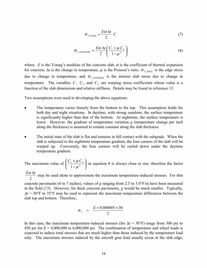
Eα ∆tσ T ,EDGE = C (7)2

σ = Eα ∆t C1 + µC2 (8)T ,INTERIOR 2

1 − µ 2

where: E is the Young’s modulus of the concrete slab, α is the coefficient of thermal expansion for concrete, ∆t is the change in temperature, µ is the Poisson’s ratio, σ T ,EDGE is the edge stress

due to change in temperature, and σ T ,INTERIOR is the interior slab stress due to change in

temperature. The variables C , C1 , and C2 are warping stress coefficients whose value is a function of the slab dimensions and relative stiffness. Details may be found in reference 13.

Two assumptions were used in developing the above equations:

• The temperature varies linearly from the bottom to the top. This assumption holds for both day and night situations. In daytime, with strong sunshine, the surface temperature is significantly higher than that of the bottom. At nighttime, the surface temperature is lower. However, the gradient of temperature variation g (temperature change per inch along the thickness) is assumed to remain constant along the slab thickness.

• The initial state of the slab is flat and remains in full contact with the subgrade. When the slab is subjected to the nighttime temperature gradient, the four corners of the slab will be warped up. Conversely, the four corners will be curled down under the daytime temperature gradient.

The maximum value of

C1 + µ 2

C2 in equation 8 is always close to one; therefore the factor

1 − µ Eα ∆t

may be used alone to approximate the maximum temperature-induced stresses. For thin 2

concrete pavements (6 to 7 inches), values of g ranging from 2.5 to 3.0°F/in have been measured in the field [13]. However, for thick concrete pavements, g would be much smaller. Typically, ∆t = 30°F to 35°F may be used to represent the maximum temperature differences between the slab top and bottom. Therefore,

E × 0.000005 × 30σ T ≈ 2

In this case, the maximum temperature-induced stresses (for ∆t = 30°F) range from 300 psi to 450 psi for E = 4,000,000 to 6,000,000 psi. The combination of temperature and wheel loads is expected to induce total stresses that are much higher than those induced by the temperature load only. The maximum stresses induced by the aircraft gear load usually occur at the slab edge,

16

while the maximum stresses induced by temperature usually occur at some distance from the edge of the slab. Combined effects of the two types of stresses should be analyzed to determine the effects of slab size when temperature variation is considered.

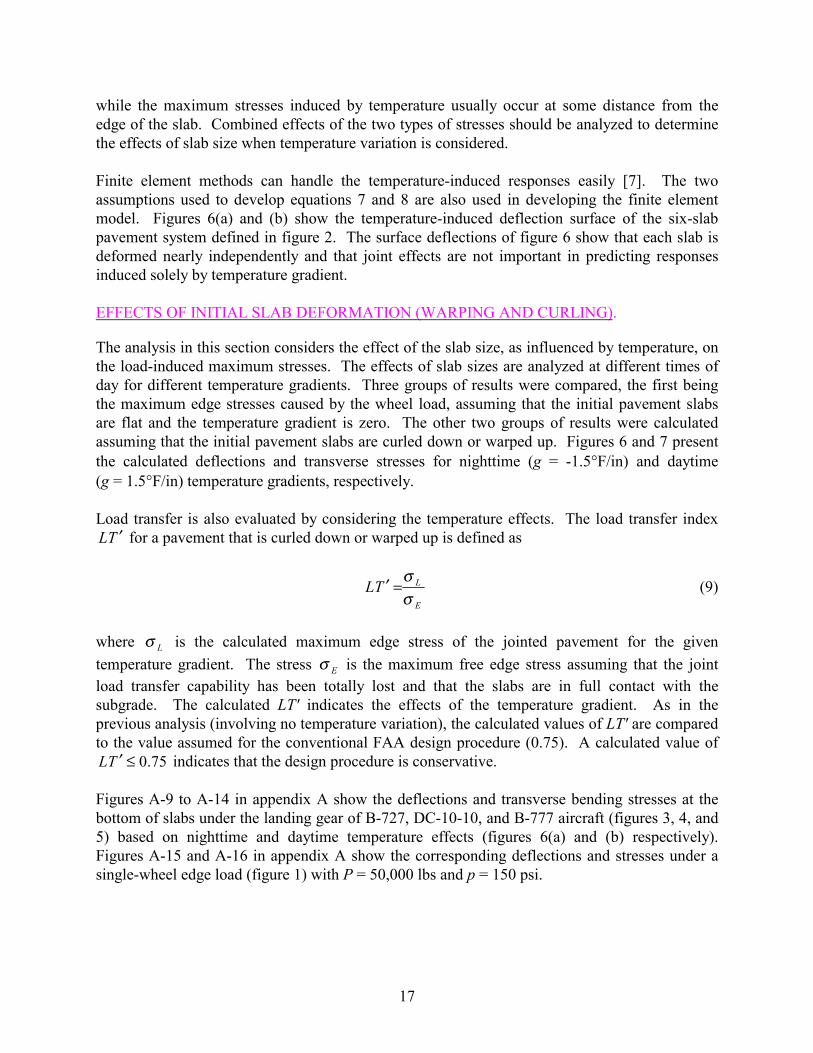
Finite element methods can handle the temperature-induced responses easily [7]. The two assumptions used to develop equations 7 and 8 are also used in developing the finite element model. Figures 6(a) and (b) show the temperature-induced deflection surface of the six-slab pavement system defined in figure 2. The surface deflections of figure 6 show that each slab is deformed nearly independently and that joint effects are not important in predicting responses induced solely by temperature gradient.

EFFECTS OF INITIAL SLAB DEFORMATION (WARPING AND CURLING).

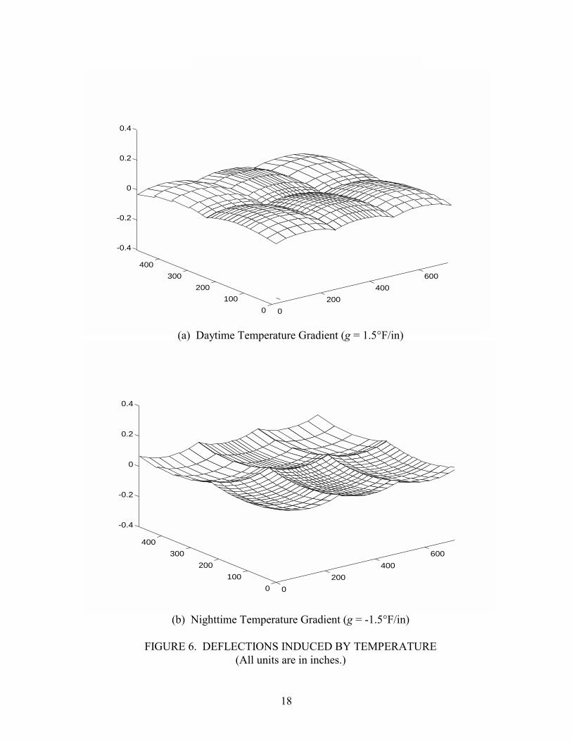
The analysis in this section considers the effect of the slab size, as influenced by temperature, on the load-induced maximum stresses. The effects of slab sizes are analyzed at different times of day for different temperature gradients. Three groups of results were compared, the first being the maximum edge stresses caused by the wheel load, assuming that the initial pavement slabs are flat and the temperature gradient is zero. The other two groups of results were calculated assuming that the initial pavement slabs are curled down or warped up. Figures 6 and 7 present the calculated deflections and transverse stresses for nighttime (g = -1.5°F/in) and daytime (g = 1.5°F/in) temperature gradients, respectively.

Load transfer is also evaluated by considering the temperature effects. The load transfer index LT ′ for a pavement that is curled down or warped up is defined as

σLT ′ =

σ L (9) E

where σ L is the calculated maximum edge stress of the jointed pavement for the given

temperature gradient. The stress σ E is the maximum free edge stress assuming that the joint load transfer capability has been totally lost and that the slabs are in full contact with the subgrade. The calculated LT' indicates the effects of the temperature gradient. As in the previous analysis (involving no temperature variation), the calculated values of LT' are compared to the value assumed for the conventional FAA design procedure (0.75). A calculated value of LT ′ ≤ 0.75 indicates that the design procedure is conservative.

Figures A-9 to A-14 in appendix A show the deflections and transverse bending stresses at the bottom of slabs under the landing gear of B-727, DC-10-10, and B-777 aircraft (figures 3, 4, and 5) based on nighttime and daytime temperature effects (figures 6(a) and (b) respectively). Figures A-15 and A-16 in appendix A show the corresponding deflections and stresses under a single-wheel edge load (figure 1) with P = 50,000 lbs and p = 150 psi.

17

18

0

200

400

600

0

100

200

300

400

-0.4

-0.2

0

0.2

0.4

inch

es

Deflection by Day Temperature, Gradient g=1.5

(a) Daytime Temperature Gradient (g = 1.5°F/in)

0

200

400

600

0

100

200

300

400

-0.4

-0.2

0

0.2

0.4

inch

es

Deflection by Night Temperature, Gradient g=-1.5

(b) Nighttime Temperature Gradient (g = -1.5°F/in)

FIGURE 6. ECTIONS INDUCED BY TEMPERATURE(All units are in inches.)

DEFL

19

0

200

400

600

0

100

200

300

400

-100

0

100

200

300

400

500

inchesinches

psi

Temperature Induced Transverse Stresses at g = -1.5 F/inch

(a) Nighttime (g = -1.5°F/inch)

0

200

400

600

0

100

200

300

400

-100

0

100

200

300

400

500

inchesinches

psi

Temperature Induced Transverse Stresses at g = 1.5 F/inch

0

200

400

600

0

100

200

300

400

-100

0

100

200

300

400

500

inchesinches

psi

Temperature Induced Transverse Stresses at g = 1.5 F/inch

(b) Daytime (g = -1.5°F/inch)

FIGURE 7. ERATURE-INDUCED TRANSVERSE STRESSESTEMP

Figures A-17 and A-18 in appendix A show the comparison of deflections at the transverse joint on the loaded and unloaded sides (figure 2) due to the loads of the B-727, DC-10-10, and B-777 landing gears configured as in figures 3, 4, and 5 respectively. Temperature effects have been simulated by using g = -1.5°F/in, g = 0, and g = 1.5°F/in. Figures A-19 and A-20 show the comparison of edge stresses on the two sides of transverse joint induced by the above aircraft landing gears at different times. All results presented in figures A-19 and A-20 were calculated using a slab width equal to 20 feet.

Table 9 compares the results of JSLAB-92 analyses involving various slab widths and relative stiffnesses. The table lists (a) maximum load-induced deflections and (b) maximum transverse stresses for the various cases, both with and without consideration of temperature-induced initial pavement states. The following cases from table 3 were incorporated in table 9: ID numbers AC1, AC2, AC3, BC1, BC2, BC3, CC1, CC2, and CC3. The notation DT is used to indicate the deflection ratio on two sides of the joint:

δ DT = U ,max (10)

δ L,max

where δU ,max and δ L,max are the maximum deflections at the joint on the unloaded and loaded side.

In pavement engineering, a number of different techniques are available to measure δU ,max and

δ L,max directly. For example, the falling weight deflectometer (FWD) is commonly used to

measure the maximum deflection on two sides of the joint. The joint load transfer efficiency is then computed from the FWD measurements.

The results in figures A-9 through A-20 and table 9 may be summarized as follows:

• The maximum deflections caused by applying loads with daytime and nighttime temperature gradients (g = 1.5 and -1.5°F/in respectively) are always larger than those for loads applied with a flat initial state (g = 0). This result is due to the existence of a gap between the slab and supporting system when g ≠ 0. At night the deflection is the highest since the slab is warping down and the effect of the load is to add to this downward warping.

• Figures A-17 and A-18 show the variation of joint deflections under three different aircraft landing gears at night and during the day for the case of l = 50. The nighttime maximum deflections (g = -1.5°F/in) are significantly greater than the deflections at other times (g = 0 or g = 1.5°F/in). This observation holds for all pavements with strong supporting systems, as shown in table 9(a). The stronger the supporting system (the smaller the value of l), the larger the difference between the night and day deflections will be, all else being equal.

20

TABLE 9. LOAD-INDUCED RESPONSES AND JOINT TRANSFER INDICES BASED ON DIFFERENT INITIAL STATES

(a) Maximum Deflection

Width = 15 ft max,Lδ (mils) max,

max,

L

UDT δ

δ =

l AGG/kl g = -1.5 g = 0 g = 1.5 g = -1.5 g = 0 g = 1.5 39 50 83

5.1 7.3 24.3

25.2 25.6 34.2

13.6 15.7 31.5

16.0 17.2 33.7

0.87 0.88 0.91

0.76 0.80 0.90

0.79 0.81 0.91


max,

L

UDT δ

δ =

l AGG/kl g = -1.5 g = 0 g = 1.5 g = -1.5 g = 0 g = 1.5 39 50 83

5.1 7.3 24.3

24.2 24.2 34.0

13.2 15.5 32.6

16.5 18.7 32.6

0.86 0.87 0.91

0.75 0.80 0.91

0.80 0.83 0.91


max,

L

UDT δ

δ =

l AGG/kl g = -1.5 g = 0 g = 1.5 g = -1.5 g = 0 g = 1.5 39 50 83

5.1 7.3 24.3

23.4 23.0 34.1

13.0 15.2 32.6

15.7 18.9 32.7

0.86 0.87 0.91

0.75 0.80 0.91

0.79 0.84 0.91

(b) Maximum Transverse Stresses Width = 15 ft max,Lσ (psi) TL ′ l AGG/kl g = -1.5 g = 0 g = 1.5 g = -1.5 g = 0 g = 1.5

39 50 83

5.1 7.3 24.3

351.8 311.3 302.1

355.9 319.6 307.5

379.8 331.8 303.1

0.75 0.73 0.71

0.76 0.75 0.72

0.81 0.78 0.71

Width = 20 ft max,Lσ (psi) TL ′ l AGG/kl g = -1.5 g = 0 g = 1.5 g = -1.5 g = 0 g = 1.5

39 50 83

5.1 7.3 24.3

350.3 308.3 309.8

352.1 315.8 312.7

376.9 336.4 312.7

0.76 0.74 0.71

0.76 0.75 0.72

0.82 0.80 0.72

Width = 25 ft max,Lσ (psi) TL ′ l AGG/kl g = -1.5 g = 0 g = 1.5 g = -1.5 g = 0 g = 1.5

39 50 83

5.1 7.3 24.3

355.9 309.5 310.4

352.2 313.5 314.1

367.1 332.8 314.4

0.77 0.75 0.71

0.77 0.76 0.72

0.80 0.81 0.72

21

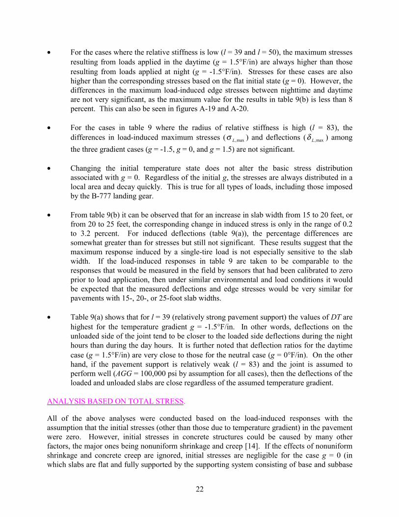
• For the cases where the relative stiffness is low (l = 39 and l = 50), the maximum stresses resulting from loads applied in the daytime (g = 1.5°F/in) are always higher than those resulting from loads applied at night (g = -1.5°F/in). Stresses for these cases are also higher than the corresponding stresses based on the flat initial state (g = 0). However, the differences in the maximum load-induced edge stresses between nighttime and daytime are not very significant, as the maximum value for the results in table 9(b) is less than 8 percent. This can also be seen in figures A-19 and A-20.

• For the cases in table 9 where the radius of relative stiffness is high (l = 83), the differences in load-induced maximum stresses (σ L,max ) and deflections (δ L,max ) among

the three gradient cases (g = -1.5, g = 0, and g = 1.5) are not significant.

• Changing the initial temperature state does not alter the basic stress distribution associated with g = 0. Regardless of the initial g, the stresses are always distributed in a local area and decay quickly. This is true for all types of loads, including those imposed by the B-777 landing gear.

• From table 9(b) it can be observed that for an increase in slab width from 15 to 20 feet, or from 20 to 25 feet, the corresponding change in induced stress is only in the range of 0.2 to 3.2 percent. For induced deflections (table 9(a)), the percentage differences are somewhat greater than for stresses but still not significant. These results suggest that the maximum response induced by a single-tire load is not especially sensitive to the slab width. If the load-induced responses in table 9 are taken to be comparable to the responses that would be measured in the field by sensors that had been calibrated to zero prior to load application, then under similar environmental and load conditions it would be expected that the measured deflections and edge stresses would be very similar for pavements with 15-, 20-, or 25-foot slab widths.

• Table 9(a) shows that for l = 39 (relatively strong pavement support) the values of DT are highest for the temperature gradient g = -1.5°F/in. In other words, deflections on the unloaded side of the joint tend to be closer to the loaded side deflections during the night hours than during the day hours. It is further noted that deflection ratios for the daytime case (g = 1.5°F/in) are very close to those for the neutral case (g = 0°F/in). On the other hand, if the pavement support is relatively weak (l = 83) and the joint is assumed to perform well (AGG = 100,000 psi by assumption for all cases), then the deflections of the loaded and unloaded slabs are close regardless of the assumed temperature gradient.

ANALYSIS BASED ON TOTAL STRESS.

All of the above analyses were conducted based on the load-induced responses with the assumption that the initial stresses (other than those due to temperature gradient) in the pavement were zero. However, initial stresses in concrete structures could be caused by many other factors, the major ones being nonuniform shrinkage and creep [14]. If the effects of nonuniform shrinkage and concrete creep are ignored, initial stresses are negligible for the case g = 0 (in which slabs are flat and fully supported by the supporting system consisting of base and subbase

22

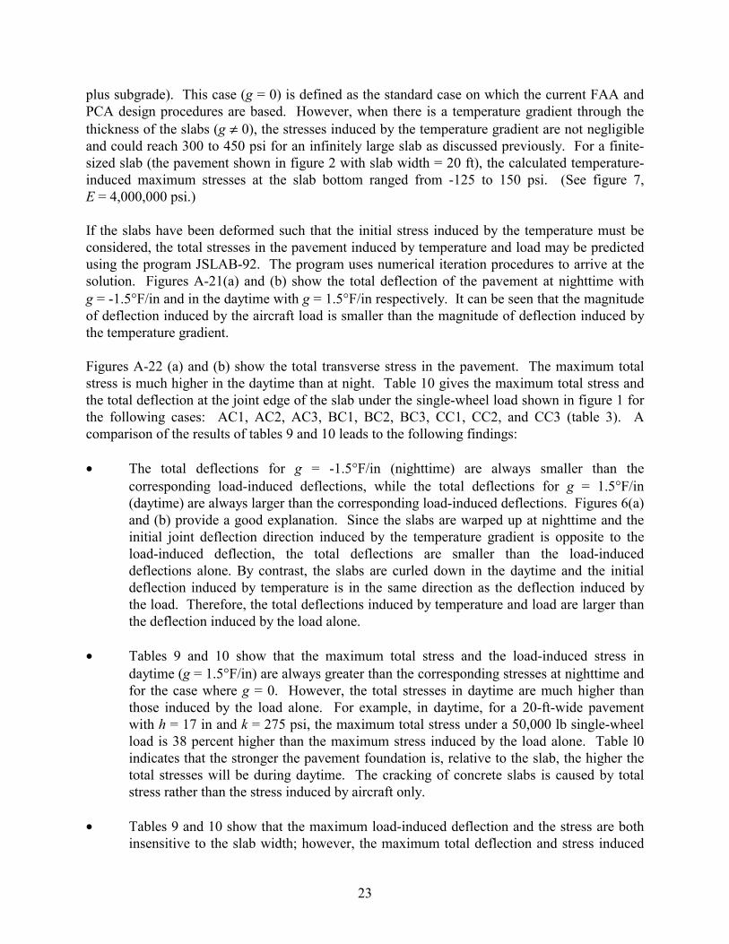
plus subgrade). This case (g = 0) is defined as the standard case on which the current FAA and PCA design procedures are based. However, when there is a temperature gradient through the thickness of the slabs (g ≠ 0), the stresses induced by the temperature gradient are not negligible and could reach 300 to 450 psi for an infinitely large slab as discussed previously. For a finite-sized slab (the pavement shown in figure 2 with slab width = 20 ft), the calculated temperature-induced maximum stresses at the slab bottom ranged from -125 to 150 psi. (See figure 7, E = 4,000,000 psi.)

If the slabs have been deformed such that the initial stress induced by the temperature must be considered, the total stresses in the pavement induced by temperature and load may be predicted using the program JSLAB-92. The program uses numerical iteration procedures to arrive at the solution. Figures A-21(a) and (b) show the total deflection of the pavement at nighttime with g = -1.5°F/in and in the daytime with g = 1.5°F/in respectively. It can be seen that the magnitude of deflection induced by the aircraft load is smaller than the magnitude of deflection induced by the temperature gradient.

Figures A-22 (a) and (b) show the total transverse stress in the pavement. The maximum total stress is much higher in the daytime than at night. Table 10 gives the maximum total stress and the total deflection at the joint edge of the slab under the single-wheel load shown in figure 1 for the following cases: AC1, AC2, AC3, BC1, BC2, BC3, CC1, CC2, and CC3 (table 3). A comparison of the results of tables 9 and 10 leads to the following findings:

• The total deflections for g = -1.5°F/in (nighttime) are always smaller than the corresponding load-induced deflections, while the total deflections for g = 1.5°F/in (daytime) are always larger than the corresponding load-induced deflections. Figures 6(a) and (b) provide a good explanation. Since the slabs are warped up at nighttime and the initial joint deflection direction induced by the temperature gradient is opposite to the load-induced deflection, the total deflections are smaller than the load-induced deflections alone. By contrast, the slabs are curled down in the daytime and the initial deflection induced by temperature is in the same direction as the deflection induced by the load. Therefore, the total deflections induced by temperature and load are larger than the deflection induced by the load alone.

• Tables 9 and 10 show that the maximum total stress and the load-induced stress in daytime (g = 1.5°F/in) are always greater than the corresponding stresses at nighttime and for the case where g = 0. However, the total stresses in daytime are much higher than those induced by the load alone. For example, in daytime, for a 20-ft-wide pavement with h = 17 in and k = 275 psi, the maximum total stress under a 50,000 lb single-wheel load is 38 percent higher than the maximum stress induced by the load alone. Table l0 indicates that the stronger the pavement foundation is, relative to the slab, the higher the total stresses will be during daytime. The cracking of concrete slabs is caused by total stress rather than the stress induced by aircraft only.

• Tables 9 and 10 show that the maximum load-induced deflection and the stress are both insensitive to the slab width; however, the maximum total deflection and stress induced

23

by temperature and load are quite sensitive to the slab width as the slab width varies from 15 to 25 ft. For example, the maximum total stress for l = 50 (h = 17 in, k = 275 pci, and E = 4,000,000 psi) in a 20-ft-wide slab pavement (figure 2) is 20 percent higher than in a 15-ft-wide slab pavement. The maximum total stress in a 25-ft-wide slab pavement is still 15 percent higher. The analysis indicates that slab width differences within a practical range of 15 to 25 ft would not significantly affect the pavement performance if only load-induced responses are assumed to be the major causes of pavement damage. However, if the critical total stresses induced by temperature and load both are assumed to be the major cause of pavement damage, the wider slab pavement would be expected to crack earlier.

TABLE 10. MAXIMUM TOTAL DEFLECTIONS, TRANSVERSE STRESSES, AND LOAD TRANSFER INDEX ( LT ′ ) FOR A 50,000 lb SINGLE-WHEEL LOAD (p = 150 psi)

A. Slab Width = 15 ft

Response max,Lδ (mils) max,Lσ (psi) TL ′

g, °F/in -1.5 0 1.5 -1.5 0 1.5 -1.5 0 1.5

l AGG/kl 2.9 0.9 11.3

13.6 15.7 31.5

21.0 27.3 55.9

315.4 283.2 289.7

355.9 319.6 307.5

471.6 388.5 316.2

0.67 0.66 0.68

0.76 0.75 0.72

1.00 0.91 0.74

39 50 83

5.1 7.3 24.3

B. Slab Width = 20 ft


g, °F/in -1.5 0 1.5 -1.5 0 1.5 -1.5 0 1.5

l AGG/kl 2.0 0.7 16.4

13.2 15.5 32.6

21.8 26.1 49.2

257.3 231.0 268.5

352.1 315.8 312.7

547.7 466.4 357.1

0.56 0.55 0.61

0.76 0.75 0.72

1.19 1.11 0.82

39 50 83

5.1 7.3 24.3

C. Slab Width = 25 ft


g, °F/in -1.5 0 1.5 -1.5 0 1.5 -1.5 0 1.5

l AGG/kl 0.6 -0.4 20.6

13.0 15.2 32.6

24.2 27.6 45.0

197.2 169.8 222.7

352.2 313.5 314.1

591.7 534.2 409.9

0.43 0.41 0.51

0.77 0.76 0.72

1.29 1.29 0.93

39 50 83

5.1 7.3 24.3

24

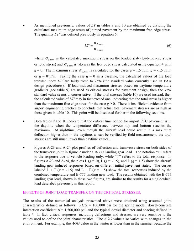
• As mentioned previously, values of LT in tables 9 and 10 are obtained by dividing the calculated maximum edge stress of jointed pavement by the maximum free edge stress. The quantity LT' was defined previously in equation 6:

σ L,maxLT' = (6)σ E,max

where σ L,max is the calculated maximum stress on the loaded slab (load-induced stress

or total stress) and σ E ,max is taken as the free edge stress calculated using equation 4 with

g = 0. The maximum stress σ L,max is calculated for the cases g = 1.5°F/in, g = -1.5°F/in,

or g = 0°F/in. Taking the case g = 0 as a baseline, the calculated values of the load transfer index LT′ are fairly close to 75% (the standard value currently used in FAA design procedures). If load-induced maximum stresses based on daytime temperature gradients (see table 9) are used as critical stresses for pavement design, then the 75% standard value seems unconservative. If the total stresses (table 10) are used instead, then the calculated value of LT' may in fact exceed one, indicating that the total stress is higher than the maximum free edge stress for the case g ≥ 0. There is insufficient evidence from airport engineering practice to conclude that actual total pavement stresses are as high as those given in table 10. This point will be discussed further in the following sections.

• Both tables 9 and 10 indicate that the critical time period for airport PCC pavement is in the daytime when the temperature difference between top and bottom reaches the maximum. At nighttime, even though the aircraft load could result in a maximum deflection higher than in the daytime, as can be verified by field measurement, the total stresses are still much lower than daytime values.

• Figures A-23 and A-24 plot profiles of deflection and transverse stress on both sides of the transverse joint in figure 2 under a B-777 landing gear load. The notation “L” refers to the response due to vehicle loading only, while “T” refers to the total response. In figures A-23 and A-24, the plots L (g = 0), L (g = -1.5), and L (g = 1.5) show the aircraft landing gear induced responses based on different initial pavement states. The curves labeled L + T (g = -1.5) and L + T (g = 1.5) show the total responses induced by the combined temperature and B-777 landing gear load. The results obtained with the B-777 landing gear load, shown in these two figures, are similar to the results for a single-wheel load described previously in this report.

EFFECTS OF JOINT LOAD TRANSFER ON THE CRITICAL STRESSES.

The results of the numerical analysis presented above were obtained using assumed joint characteristics defined as follows: AGG = 100,000 psi for the spring model, dowel-concrete interaction coefficient α = 1,500,000 pci, and the typical dowel diameter and spacing defined in table 4. In fact, critical responses, including deflections and stresses, are very sensitive to the values used to define the joint characteristics. The AGG value also varies with changes in the environment. For example, the AGG value in the winter is lower than in the summer because the

25

lower average temperature in winter shortens the slab length and leads to larger joint openings. The larger joint openings tend to reduce the joint load transfer capability. In the summer, the load transfer capability is higher.

The following cases in table 3 were selected to represent strong, medium, and weak pavement supporting systems: CA1, AA1, and BA1. The spring model was used to define the joint load transfer. The values of AGG used for investigating the effects of the joint characteristics varied from 1,940 to 1,000,000 psi. The dimensionless joint parameter AGG/kl defined in reference 12 ranges from 0.1 to 241. The higher AGG/kl value indicates a stronger joint relative to the pavement supporting system.

Figure 8(a) plots LT (the fraction of the total load transferred through the joint) as a function of the dimensionless joint parameter AGG/kl. The findings are summarized below.

• The load transfer as measured by LT is very sensitive to the dimensionless joint parameter. The higher the value of AGG/kl, the more load will be transferred through the joint.

• FAA design procedures assume that 25 percent of the total load is transferred through the joint. Based on figure 8(a), this assumption would place the parameter AGG/kl in the range from 5.1 to 12.1.

• The relationship between LT and AGG/kl is influenced slightly by the value of a/l, which is a dimensionless parameter related to tire pressure. All else being equal, a higher tire pressure will result in a larger difference between the maximum stress on two sides of the joint.

Figure 8(b) shows the deflection ratio (DT) of the joint as a function of AGG/kl. DT is defined by equation 10. The findings are summarized below.

• The higher the value of AGG/kl, the higher the deflection load transfer efficiency.

• For LT = 0.25, DT is in the range 0.43 to 0.46.

• DT is mainly determined by the dimensionless parameter AGG/kl and is insensitive to a/l. A comparison between figures 8(a) and (b) indicates that LT is more sensitive than DT to a/l.

26

LT

0.5

a/l=0.124

a/l=0.206

a/l=0.264

LT = 0.25

0.4

0.3

0.2

0.1

AGG/kl0

0.1

DT

5.1 12.110 1000

(a) LT as a function of AGG/kl

1

.85

0.8 .75

0.6

0.4

0.2

a/l=0.124 a/l=0.206 a/l=0.264

0 AGG/kl

5.1 12.1 0.1 10 1000

(b) DT as a function of AGG/kl

FIGURE 8. COMPUTED LOAD TRANSFER AS A FUNCTION OF THE DIMENSIONLESS JOINT PARAMETER

SUMMARY OF FINDINGS.

• The calculated critical responses, which are currently used to estimate the remaining life of pavements, are significantly influenced by the effects of slab size on PCC pavement

27

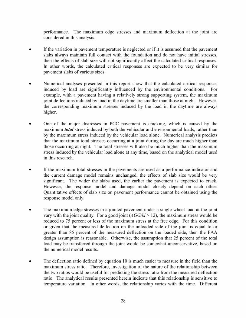
performance. The maximum edge stresses and maximum deflection at the joint are considered in this analysis.

• If the variation in pavement temperature is neglected or if it is assumed that the pavement slabs always maintain full contact with the foundation and do not have initial stresses, then the effects of slab size will not significantly affect the calculated critical responses. In other words, the calculated critical responses are expected to be very similar for pavement slabs of various sizes.

• Numerical analyses presented in this report show that the calculated critical responses induced by load are significantly influenced by the environmental conditions. For example, with a pavement having a relatively strong supporting system, the maximum joint deflections induced by load in the daytime are smaller than those at night. However, the corresponding maximum stresses induced by the load in the daytime are always higher.

• One of the major distresses in PCC pavement is cracking, which is caused by the maximum total stress induced by both the vehicular and environmental loads, rather than by the maximum stress induced by the vehicular load alone. Numerical analysis predicts that the maximum total stresses occurring at a joint during the day are much higher than those occurring at night. The total stresses will also be much higher than the maximum stress induced by the vehicular load alone at any time, based on the analytical model used in this research.

• If the maximum total stresses in the pavements are used as a performance indicator and the current damage model remains unchanged, the effects of slab size would be very significant. The wider the slabs used, the earlier the pavement is expected to crack. However, the response model and damage model closely depend on each other. Quantitative effects of slab size on pavement performance cannot be obtained using the response model only.

• The maximum edge stresses in a jointed pavement under a single-wheel load at the joint vary with the joint quality. For a good joint (AGG/kl > 12), the maximum stress would be reduced to 75 percent or less of the maximum stress at the free edge. For this condition or given that the measured deflection on the unloaded side of the joint is equal to or greater than 85 percent of the measured deflection on the loaded side, then the FAA design assumption is reasonable. Otherwise, the assumption that 25 percent of the total load may be transferred through the joint would be somewhat unconservative, based on the numerical model results.

• The deflection ratio defined by equation 10 is much easier to measure in the field than the maximum stress ratio. Therefore, investigation of the nature of the relationship between the two ratios would be useful for predicting the stress ratio from the measured deflection ratio. The analytical results presented herein indicate that this relationship is sensitive to temperature variation. In other words, the relationship varies with the time. Different

28

equations would be needed to predict the stress ratio by the measured deflection ratio for day and night conditions.

• While the analysis concludes that wider slabs will crack earlier, this conclusion is preliminary. Many factors, some of which may have a significant influence on the accuracy of the analytical results, exist in the analytical model. The following are some important considerations for future analyses:

− In the present analysis, the temperature gradient is always assumed linear. In fact, the temperature gradient is not linear in general and varies with time.

− The pavement is modeled using a slab-on-springs system, but the behavior of the material under the slab is much more complicated than the system of elastic springs. In particular, the foundation model used cannot consider the effect of load transfer in shear through the foundation layers.

− The slabs are assumed free to move in plane. This assumption has significant effect on the maximum temperature-induced stresses.

• Performance of the pavement cannot be predicted directly by the calculated critical response in the slabs. The performance of the pavement is influenced by a combination of many factors and it cannot be reproduced by any available simplified models. Therefore, airport survey data and information derived from the experiences of pavement engineers working at airports must be used to verify the results obtained from theoretical analyses intended to identify appropriate slab sizes.

PART TWO: STATISTICAL ANALYSIS OF FIELD SURVEYED DATA

INTRODUCTION.

The analytical results presented in part one indicate that the larger the PCC slabs, the earlier the cracks occur in the slabs, if total stress is taken as the major pavement damage indicator. However, the analysis was conducted based on many assumptions. For example, the temperature gradient through the slab thickness was assumed to be linear, and the temperature-induced bending stresses in the middle plane of the slab always remain at zero. Also, it was assumed that the bending stresses are zero everywhere in the slabs if the temperature gradient is zero and there is no aircraft load acting on the slabs. These assumptions are extremely important in deriving the analytical formulas, since the assumptions simplify the procedure for predicting pavement responses. Many uncertainties in predicting pavement responses have been neglected by introducing these assumptions.

Another assumption used in the analysis was that the maximum bending response may be used as an indicator to predict pavement performance under a certain number of repetitions of the maximum responses. However, the maximum bending stress is not a good indicator for some distresses. For example, joint and corner spalling are not closely related to the maximum

29

bending stress. Infiltration of incompressible materials into the joint and horizontal slab movement due to increase of temperature could produce very high compressive stress in the concrete near the joint. The combination of these stresses and stresses due to traffic load, sometimes with weak concrete due to overworking, may cause joint and corner spalling.

The following phenomena have been observed and/or recognized [15]:

• The concept of fatigue failure has been a good criterion for pavement design. However, pavements rarely, if at all, fail as a result of aircraft loading alone during their service life. Some PCC pavements, aged between 1 to 3 years, have been observed to have serious cracks. In these cases, fatigue damage was ruled out as a cause of early cracking. Field observation of pavements in service showed that the pavement distresses are caused by factors which are much more complex than those currently considered in any analytical models.

• Pavement slabs have been observed to undergo upward warping during concrete hardening. This warping remains as a permanent deformation and influences the total stress in the slabs, continuing to affect the pavement performance during its service period. Since the shape of the initial warping depends on the air temperature, water content of the concrete, and type of cement, it would be a random variable rather than a constant for all pavement slabs. Therefore, it is almost impossible to predict precisely a generic pavement response at any time using deterministic mathematical tools.

• It is important to distinguish the concept of pavement performance from the analytically computed pavement response. The former is more complex than the latter for two reasons:

− Pavement performance is not as clearly defined as pavement response. Usually, response is defined as the change in the value of one variable (e.g., deflection, strain, or stress) at a specific location in the pavement structure, due to one or more known external loads (vehicular or temperature loading). In contrast, there is no universally accepted definition of pavement performance, which depends on visual evaluations of accumulated distresses and estimates of remaining pavement life.

− In general, pavement response is an objective concept since it can be measured directly. By contrast, some aspects of pavement performance (such as pavement distresses) must be evaluated visually by a human expert so that the results are necessarily subjective. Although much progress has been made toward achieving a more objective evaluation of pavement distresses, a practical means of applying these techniques is not yet available.

The current FAA design procedure for PCC airport pavements has implicitly considered the effects of temperature variation [1, 16]. The design procedure may be divided into two steps. The first step calculates the critical stress (σ) in the pavement slab. The second step predicts the

30

repetitions of load (N) that will cause the pavement to reach a specified level of damage. This determination is made through the use of N-σ curves that were developed based on full-scale tests. Though temperature effects have not been considered explicitly in calculating the critical stress under the load, the N-σ curves in the design procedure implicitly consider the effects of weather. Because the tests on which the curves are based lasted for days, weeks, or even months, the effects of temperature variation on the pavement damage are implicitly included. For example, if two pavement sections (A and B) are structurally identical and both are subjected to the same vehicular loads, but section A experienced much larger temperature variations than B, then section A would need fewer repetitions than B to reach the same degree of damage. However, it is very difficult to quantitatively evaluate the component in the design model that is due to the temperature effects.

In this section, the effects of PCC pavement slab size are evaluated by statistical analysis of the PCI values [17]. A large quantity of existing PCI data has been analyzed to answer the following questions: Do larger slabs generally cause a larger reduction of PCI over a given period of time than smaller slabs? If the answer to this question is affirmative, then is it true for all functional pavements (apron, taxiway, and runway)? PCI data was surveyed for approximately 288 million square feet of PCC runway, taxiway, and apron pavements from 174 airports located in 23 U.S. states and Japan.

STATISTICAL CONCEPTS USED IN THE ANALYSIS.

The effects of PCC slab size on pavement performance cannot be established by theoretical analysis only. Statistical analysis based on a large quantity of data is the best procedure to investigate the subject because:

• Factors which cannot be considered appropriately or completely in a theoretical context are considered in the statistical analysis because the data are collected from operational pavements experiencing the effects of the factors.

• Statistical uncertainties may be reduced to a low level if the number of samples is large enough.

In probability theory, the probabilistic properties of a random variable X may be completely described by its probability distribution function. The PCI of pavements may be defined as a random variable affected by many factors. However, it is difficult to find the correct probability distribution function for PCI considered as a random variable.

In 1990, 5595 public airports were in operation worldwide [18] and these comprise the data group (population) for airport pavements. For such a large group, it is reasonable to estimate the probabilistic properties by analyzing the data in a selected sample group that is much smaller than the entire global group. The two most useful statistics for data analysis are the sample mean:

31

n

∑ X i

µ X = i=1 (12) n

and the standard deviation:

σ X = 1

1

2

−

− ∑=

n

)X ( n

i i µ

(13)

In the above two equations, n is the size of the sample selected at random from the population. The standard deviation indicates how the sample data are distributed around the mean. Reference 19 is a good general reference for statistical analysis procedures and basic concepts.

If the size of the population N is equal to the sample size n (in other words, if all available data were used), then the sample mean and standard deviation are equal to the mean and standard deviation respectively of the population. However, if n < N, the mean of selected samples will also be a random variable Y [19]. The mean of Y is

µY =µX (14)

and the standard deviation of Y is

σ Y =σ X × ) N ( n

n N

1− ×

− (15)

The more data that are used, the more reliable the statistical analysis will be.

In this report, the mean value of PCI is used to indicate the pavement condition, and the ratio of the standard deviation to the mean (coefficient of variance, COV) is used to estimate the reliability of the results. One typical application of the COV is to group the data to obtain meaningful results.

ASSUMPTIONS USED IN THE ANALYSIS.

Pavement survey data were collected from a variety of sources to cover different environmental, traffic, and age conditions. Data used in the statistical analysis were collected by different consulting companies, airport authorities, and agencies. About three-quarters of the data used (as measured by the number of features) were provided by Eckrose/Green Associates, who conducted a search of all of their available existing database files developed since 1985 [20 and 21]. The remaining data were provided by Harding Lawson Associates and Pavement Consultants, Inc. [22], Roy D. McQueen Associates [23, 24, and 25], and collected from reports prepared by ERES Consultants, Inc. [26].

32

The surveyed PCI results are influenced by many factors. For example, the results are affected by the original design of the pavement sections. If the original design was overly conservative, the surveyed PCIs could be higher than those surveyed for less conservatively designed pavement sections. The PCIs are also affected by the level of maintenance conducted since the pavement sections were put into service. Variation in the rehabilitation quality makes the PCI data more difficult to interpret. Furthermore, the surveys were done by different personnel from different companies, with each company’s personnel following a slightly different survey procedure, (although all the surveys essentially followed the FAA Advisory Circular 150/5380-6 [17]). In lieu of a detailed and complicated analysis that would explicitly consider all of the above factors, the following assumptions have been made:

• All surveyed pavement sections were designed properly with a design life of 20 years.

• All surveyed pavement sections have been properly maintained.

• PCC overlaid sections are treated the same as new PCC pavement and the age is counted from the time of the overlay construction.

• All subjective effects of surveyors on the PCI results are neglected in the statistical analysis.

GENERAL SURVEY INFORMATION.

The analysis included 288.4 million square feet (msf) of pavement data from 2820 features of 174 airports. These airports are located in 23 states (6 FAA regions and Hawaii) and one airport in Japan; three of the airports are military airports. The three military airports are the Marine Corps Air Stations Futenma (OTM), Okinawa, Japan; Kaneohe Bay (KAN), Hawaii; and El Toro (NZJ), California. The number of features and corresponding areas of the pavements in each state and FAA region are listed in table 11.

33

34

TABLE 11. STRIBUTION OF PAVEMENTS

Region/Location State Airport No. and ID

Number ofFeatures

Total Area(msf)

Eastern 4 4 106 24.89(EA) DC IAD 96 22.37

NJ ACY 5 0.96NY SCH 2 0.70PA PIT 3 0.86

Great 6 98 1055 100.73Lakes(GL)

IN 012, 2IN, 4I8, BAK, CEV, EVV, FWA, HUF, I14, IND, LAF,MIE, MQJ, OKK, SER

192 15.49

MI 1D2, 2G5, 3TR, 55D, 5D8, 76G, 7D2, APN, BEH, BTL, CIU,D92, D96, D98, DET, FNT, GRR, JXN, LAN, UIZ, Y66

111 11.42

MN 04Y, 27D, AXN, BJI, BRD, CKN, DLH, ELO, FFM, HIB, ILL,INL, MKT, ONA, OTG, RGK, RST, ULM, Y68

100 6.55

ND 05D, 20U, 2D5, 5N8, 6D8, 95D, BIS, BWP, DVL, FAR, GFK,ISN, JMS, MOT, N22, N55

238 17.21

SD 1D1, ABR, ATY, FSD, HON, MHE, PIR, RAP, YKN 66 7.98WI ATW, AUW, C85, CMY, CWA, EAU, ENW, FLD, GRB, ISW,

JVL, LSE, MKE, MSN, OSH, RAC, RHI, STE348 42.08

New 2 3 61 13.37York MA BED, BOS 38 6.93(NE) ME BGR 23 6.44

Southern 4 52 529 65.97(SO) FL 34J, 40J, 42J, 55J, AAF, APF, BCT, BKV, BOW, COT, CTY,

DAB, DED, FLL, GNV, IMM, ISM, JAX, LAL, LEE, MAI,MKY, MLB, MTH, OMN, OPF, PBI, PFN, PGD, PIE, PNS,RSW, SEF, SFB, SRQ, TLH, TPA, VNC, VPS, VRB, VRB,X14, X21, X35, X47, X51, X60, ZPH

409 45.84

KY CVG, PWM 67 13.76NC RDU 35 4.19TN BNA 18 2.18

Southwest 3 5 787 51.55(SW) LA HUM 36 3.45

OK TUL 198 14.53TX ADS, DFW, ELP 553 33.57

Western- 3 10 214 26.37Pacific AZ IWA, YUM 105 14.88

WP CA NZJ 100 11.24NV 4SD, BAM, EKO, ELY, LOL, MEV, WMC 9 0.25

Hawaii 1 1 44 2.2HI HI KAN 44 2.2

JAPAN 1 1 (FUT) 24 3.25Summary: 23 States plus Japan, 2820 Features, 288.4 msf

DI

��

��

��

��

��

��

��

��

��

��

��

��

��

��

��

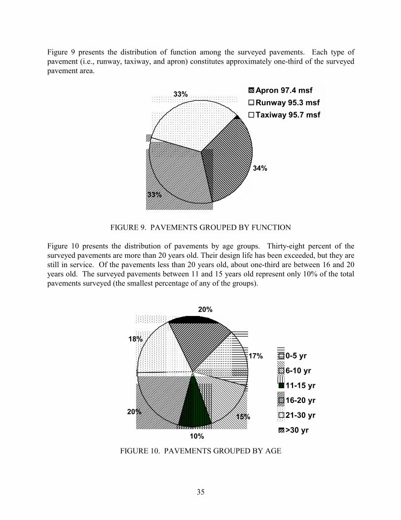
Figure 9 presents the distribution of function among the surveyed pavements. Each type of pavement (i.e., runway, taxiway, and apron) constitutes approximately one-third of the surveyed pavement area.

��

��

��

33%

34%

33% �� Apron 97.4 msf �� Runway 95.3 msf

Taxiway 95.7 msf

FIGURE 9. PAVEMENTS GROUPED BY FUNCTION

Figure 10 presents the distribution of pavements by age groups. Thirty-eight percent of the surveyed pavements are more than 20 years old. Their design life has been exceeded, but they are still in service. Of the pavements less than 20 years old, about one-third are between 16 and 20 years old. The surveyed pavements between 11 and 15 years old represent only 10% of the total pavements surveyed (the smallest percentage of any of the groups).

20%

��

��

��

��

��

18%

20% 15%

��17% 0-5 yr

�� 6-10 yr

�� 11-15 yr �� 16-20 yr

�� 21-30 yr

�� >30 yr10%

FIGURE 10. PAVEMENTS GROUPED BY AGE

35

��

��

��

��

��

Figure 11 divides the pavements in this study into groups according to the year that they were built. As shown in figure 11, 16 percent of the pavements analyzed were built in the last 10 years, less than the percentage built between 1977 and 1986 (24%) and between 1967 and 1976 (26%). The remaining pavements (34%) were built prior to 1967. New pavements were not included in this study since PCI for new pavements is generally equal to 100 and slab size information for recently built pavements is not available in the existing database.

34%

16%

��

��

��

24%

26%

��

��

��

1987-96

1977-86

1967-76

Before 1967

FIGURE 11. PAVEMENTS GROUPED BY YEAR BUILT

Because many features of pavements in airports have curved edges, the size of the slab is usually calculated by dividing the measured area of the feature by the number of slabs in the feature rather than by measuring the slab directly. For some features, especially in the apron areas of airports, slab size and shapes can vary. Therefore, the average size of the slabs is used instead of the true size of each slab.

Figure 12 shows the distribution of pavements grouped by average slab size. Fifty-five percent of the total used data come from the slabs smaller than 500 square feet. Most of the slabs in the 500 to 625 sq. ft. group are 25 by 20 ft or 25 by 25 ft, the maximum joint spacing recommended in reference 1. Only 5 percent of the slabs are greater than 625 sq. ft.

A second way of defining the slab group is by classifying according to the smallest slab length. For example, a 100-sq. ft. slab usually has a 10 ft length for two sides. Similarly, a 125-sq. ft. slab is usually sized as 10 by 12.5 ft, a 150-sq. ft. slab is 10 by 15 ft, and a 200-sq. ft. slab is 10 by 20 ft, etc. Although their areas are different, their smallest side lengths are the same. Based on the theoretical analysis in part one of this report, the maximum total bending stresses caused by aircraft loading and temperature variation are more sensitive to the smallest length of a side than to the area of the slabs. For example, the total bending stress of a 20- by 25-ft slab is close to that of a 20- by 20-ft slab if a single wheel is applied at the 20-ft edge. Table 12 groups the

36

��

��

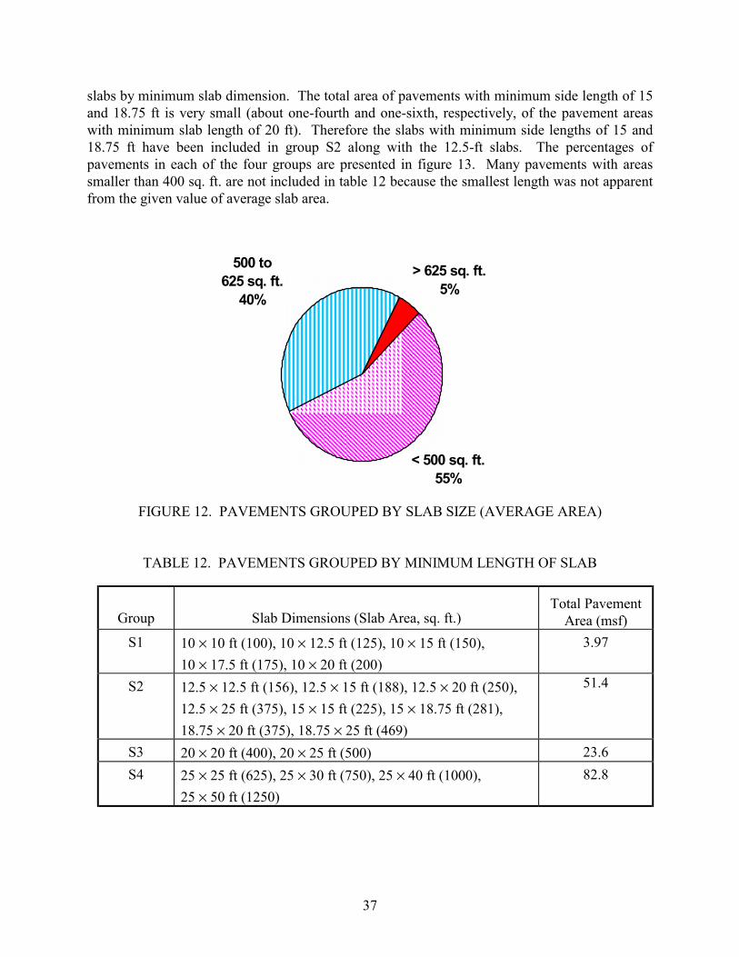
slabs by minimum slab dimension. The total area of pavements with minimum side length of 15 and 18.75 ft is very small (about one-fourth and one-sixth, respectively, of the pavement areas with minimum slab length of 20 ft). Therefore the slabs with minimum side lengths of 15 and 18.75 ft have been included in group S2 along with the 12.5-ft slabs. The percentages of pavements in each of the four groups are presented in figure 13. Many pavements with areas smaller than 400 sq. ft. are not included in table 12 because the smallest length was not apparent from the given value of average slab area.

500 to > 625 sq. ft. 625 sq. ft.

40%��

��

5%

< 500 sq. ft. 55%

FIGURE 12. PAVEMENTS GROUPED BY SLAB SIZE (AVERAGE AREA)

TABLE 12. PAVEMENTS GROUPED BY MINIMUM LENGTH OF SLAB

Group Slab Dimensions (Slab Area, sq. ft.) Total Pavement

Area (msf)

S1 10 × 10 ft (100), 10 × 12.5 ft (125), 10 × 15 ft (150),

10 × 17.5 ft (175), 10 × 20 ft (200)

3.97

S2 12.5 × 12.5 ft (156), 12.5 × 15 ft (188), 12.5 × 20 ft (250),

12.5 × 25 ft (375), 15 × 15 ft (225), 15 × 18.75 ft (281),

18.75 × 20 ft (375), 18.75 × 25 ft (469)

51.4

S3 20 × 20 ft (400), 20 × 25 ft (500) 23.6

S4 25 × 25 ft (625), 25 × 30 ft (750), 25 × 40 ft (1000),

25 × 50 ft (1250)

82.8

37

��

��

��

��

��

��

��

S1 2%

S4 51%

S315%

S232%

FIGURE 13. PAVEMENT GROUPED BY MINIMUM SLAB DIMENSION

A statistical analysis was performed for the four groups in table 12. The results of this analysis are presented in the remainder of the report.

DATA SELECTION.

Since the size of features varies, the statistical calculation of PCI should consider the effects of feature size. The following equations are used to calculate mean value and standard deviation weighted by the feature size.

n ∑ PCIi Ai

n

PCI AVG = i=1 n

=∑ PCIi

n

Ai

(16)

i=1∑ Ai ∑ Aj i=1 j=1

n

STD =∑ (PCIi −PCI AVG )2

n

Ai

(17)

i=1

∑ Aj j =1

where Ai (∑ Aj ) may be defined as the weighting factor for feature i. If the sizes of all features

are the same, the weighting factor will be equal to 1/n where n is the total number of the features. Then the COV of the PCI can be calculated by

38

39

AVGPCI

STD=COV (18)

Prior to the analysis, the following two questions were resolved:

• Should the collected pavement data for all ages be used?• Should the collected pavement data for all sizes of airports be used?

Table 13 presents the mean, standard deviation, and coefficient of variance of PCI calculated forthree groups of data: ear-old pavements (group 1), all pavements older than 30years (group 2), and 0- to 30-year-old pavements from large, medium, and small hub airportsonly (group 3).

TABLE 13. ECTION FOR THE ANALYSIS

Group Statistic Apron Taxiway Runway Total

Area (Σ Ai, msf) 74.5 83.3 73.5 231.3

AVGPCI 82.4 85.8 88.4 85.5

STD 20.0 13.4 10.8 15.4

(1)

All 0- to 30-year-oldpavements

COV (%) 24.3 15.6 12.2 18.0

Area (Σ Ai, msf) 22.9 12.3 21.8 57.0

AVGPCI 49.7 66.5 69.7 61.0

STD 22.9 23.0 19.9 23.7

(2)

All pavements olderthan 30 years

COV (%) 46.1 34.6 28.6 38.9

Area (Σ Ai, msf) 46.5 48.9 42.8 148.3

AVGPCI 80.8 86.1 88.7 85.2

STD 20.6 13.2 10.8 15.7

(3)

0- to 30-year-oldpavements fromlarge, medium, orsmall hubs only

COV (%) 25.5 15.3 12.2 18.4

Figure 14(a) shows that, for the pavements included in the survey, those older than 30 years haveaverage PCI values much lower than the other two groups while figure 14(b) shows that thevalues of COV for group 2 are twice as high as those for group 1. values of very old pavements have more uncertainty in the data. analysis was restricted to data for pavements with ages ranging from 0 to 30 years.

Comparison between group one and group three (figure 14(a)) indicates that the average PCIvalues for these two groups are close. Likewise, the reliability of pavement data taken fromlarger airports only (group 3) and from all airports (group 1) are also very close (figure 14(b)).The above comparison justifies using pavement data from all airports rather than from hubairports only. (Large, medium, and small hubs are as defined in reference 18.)

all 0- to 30-y

DATA SEL

This indicates that the PCITherefore, the statistical

��

��

��

��

��

��

��

��

��

��

��

��

��

��

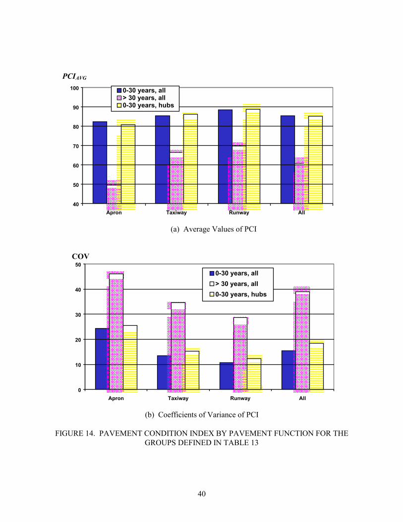
PCIAVG

100

90

80

70

60

50

40

��

��

��

��

��

��

��

��

0-30 years, all �� > 30 years, all �� 0-30 years, hubs

Apron Taxiway Runway All

(a) Average Values of PCI

COV50

40

30

20

10

0

��

��

��

��

��

��

��

��

0-30 years, all

> 30 years, all �� 0-30 years, hubs

Apron Taxiway Runway All

(b) Coefficients of Variance of PCI

FIGURE 14. PAVEMENT CONDITION INDEX BY PAVEMENT FUNCTION FOR THEGROUPS DEFINED IN TABLE 13

40

VARIATION OF PCI BY PAVEMENT TYPE AND AGE.

The average PCI values for 0- to 30-year-old pavements arranged by function are plotted in figure 15. The average PCI of runway pavements is highest and the average PCI of apron pavement is lowest, although all three types of pavement exhibit similar average PCI.

PCIAVG 100

95

90

85

80

75

70

65

60

55

50

45

40

Apron Taxiway Runway

FIGURE 15. AVERAGE PAVEMENT CONDITION INDEX FOR SURVEYED PAVEMENTS NEWER THAN 30 YEARS OLD

The average PCI values for all surveyed pavements grouped by age are shown in figure 16(a). The average PCI decreases as the age increases. Furthermore, the decrease in the PCI value for pavements older than 30 years is much higher than the decrease in the PCI value for any other group. As mentioned previously, the data for pavements older than 30 years was not included in the detailed analysis.

Figure 16(b) presents the average value of PCI grouped by age for different pavement functions (aprons, taxiways, and runways). In general the average PCI decreases as the age increases, except for 16- to 20-year-old aprons and for 11- to 15-year-old runways. For pavements within the same age group, runways generally exhibit the highest average PCI, followed by taxiways, except in the 11- to 15-year-old group. The PCI of aprons is always the lowest compared to the other two functional categories.

41

��

��

��

��

��

��

��

��

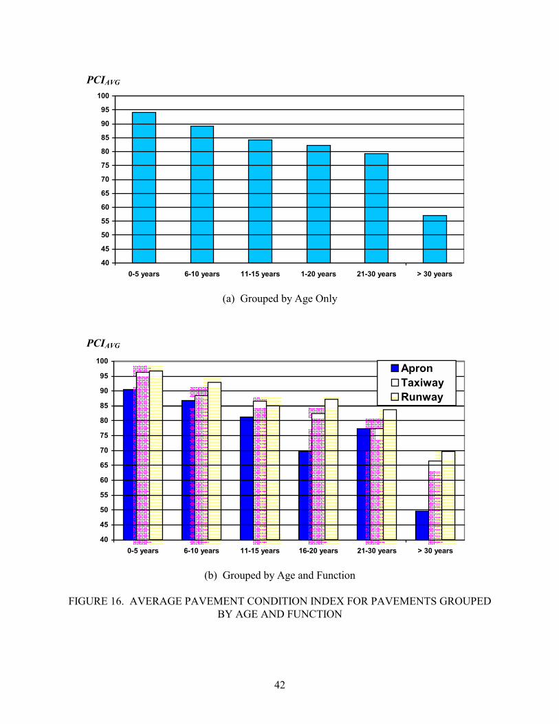
PCIAVG

100

95

90

85

80

75

70

65

60

55

50

45

40

0-5 years 6-10 years 11-15 years 1-20 years 21-30 years > 30 years

(a) Grouped by Age Only

PCIAVG

100

95

90

85

80

75

70

65

60

55

50

45

40

0-5 years 6-10 years 11-15 years 16-20 years 21-30 years > 30 years

��

��

��

��

��

��

��

��

��

��

��

��

Apron Taxiway

�� Runway

(b) Grouped by Age and Function

FIGURE 16. AVERAGE PAVEMENT CONDITION INDEX FOR PAVEMENTS GROUPED BY AGE AND FUNCTION

42

��

��

��

��

��

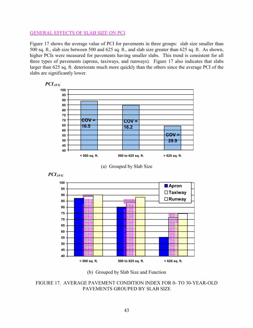
GENERAL EFFECTS OF SLAB SIZE ON PCI.

Figure 17 shows the average value of PCI for pavements in three groups: slab size smaller than 500 sq. ft., slab size between 500 and 625 sq. ft., and slab size greater than 625 sq. ft. As shown, higher PCIs were measured for pavements having smaller slabs. This trend is consistent for all three types of pavements (aprons, taxiways, and runways). Figure 17 also indicates that slabs larger than 625 sq. ft. deteriorate much more quickly than the others since the average PCI of the slabs are significantly lower.

PCIAVG

100

95

90

85

80

75

70

65

60

55

50

45

40

COV = 16.5

COV = 16.2

COV = 29.9

< 500 sq. ft. 500 to 625 sq. ft. > 625 sq. ft.

(a) Grouped by Slab Size

PCIAVG

100

95

90

85

80

75

70

65

60

55

50

45

40

��

��

��

��

��

��

Apron

Taxiway �� Runway

< 500 sq. ft. 500 to 625 sq. ft. > 626 sq. ft.

(b) Grouped by Slab Size and Function

FIGURE 17. AVERAGE PAVEMENT CONDITION INDEX FOR 0- TO 30-YEAR-OLDPAVEMENTS GROUPED BY SLAB SIZE

43

��

��

��

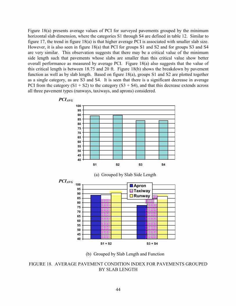
Figure 18(a) presents average values of PCI for surveyed pavements grouped by the minimum horizontal slab dimension, where the categories S1 through S4 are defined in table 12. Similar to figure 17, the trend in figure 18(a) is that higher average PCI is associated with smaller slab size. However, it is also seen in figure 18(a) that PCI for groups S1 and S2 and for groups S3 and S4 are very similar. This observation suggests that there may be a critical value of the minimum side length such that pavements whose slabs are smaller than this critical value show better overall performance as measured by average PCI. Figure 18(a) also suggests that the value of this critical length is between 18.75 and 20 ft. Figure 18(b) shows the breakdown by pavement function as well as by slab length. Based on figure 18(a), groups S1 and S2 are plotted together as a single category, as are S3 and S4. It is seen that there is a significant decrease in average PCI from the category (S1 + S2) to the category (S3 + S4), and that this decrease extends across all three pavement types (runways, taxiways, and aprons) considered.

PCIAVG

100

95

90

85

80

75

70

65

60

55

50

45

40

S1 S2 S3 S4

(a) Grouped by Slab Side Length

PCIAVG 100

95

90

85

80

75

70

65

60

55

50

45

40

S1 + S2 S3 + S4

��

��

��

��

Apron �� Taxiway ��

Runway

(b) Grouped by Slab Length and Function

FIGURE 18. AVERAGE PAVEMENT CONDITION INDEX FOR PAVEMENTS GROUPED BY SLAB LENGTH

44

45

Table 14 displays the results of individual group analyses broken down by function. It can beseen that in several individual cases, values of PCI for larger slabs are higher than those forsmaller slabs. or example, the average PCI of group S3 is higher than the average PCI ofgroups S2 and S1 for apron data. ikewise, the PCI of group S4 is higher than the PCI of groupS3 for taxiway and runway data.

TABLE 14. FOR PAVEMENTS GROUPED BY MINIMUM SLAB LENGTH

Group Total Area (msf) Average PCI Coefficient of VarianceAll Pavements

S1 3.97 88.4 13.8S2 51.4 89.2 14.7S3 23.6 83.5 13.8S4 82.8 83.4 18.8

Apron

S1 1.73 86.3 17.0S2 19.8 88.5 18.4S3 5.08 92.6 9.5S4 23.3 73.9 27.6

Taxiway

S1 1.7 87.4 10.8S2 16.5 89.0 12.4S3 8.6 77.1 15.2S4 28.4 86.1 13.4

Runway

S1 0.54 98.1 2.5S2 15.0 90.5 11.3S3 9.89 84.4 10.4S4 31.06 88.0 12.8

Although the data in table 14 do not show in every case that the PCI decreases as the slab sizeincreases, the following should be noted:

• The relatively small amount of data in groups S1 and S3 from aprons, groups S1 and S3from taxiways, and group S1 from runways might not be sufficient to provide reliablestatistical results.

• In order to compensate for the lack of available data in certain groups as noted above,groups were combined as in figure 18. y combining smaller groups into larger groupsof similar size, meaningful results for all three types of pavements were obtained.

FL

AVERAGE PCI

B

��

��

��

��

��

��

��

��

��

��

��

��

��

��

��

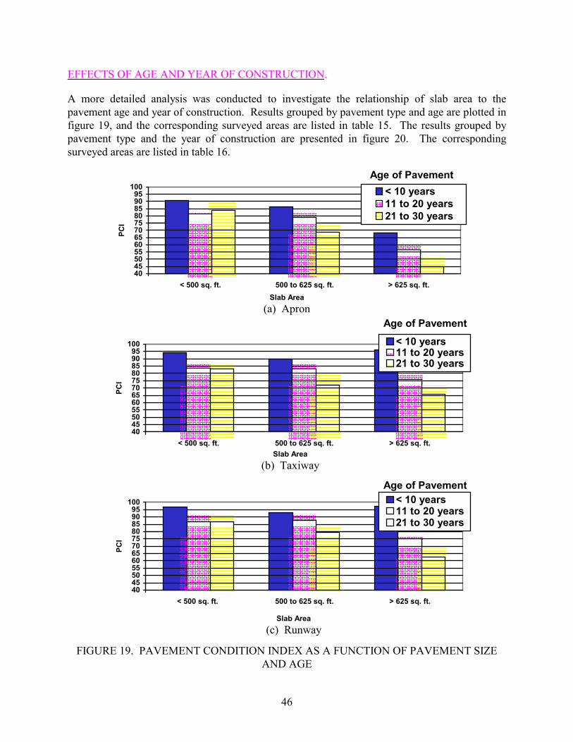
EFFECTS OF AGE AND YEAR OF CONSTRUCTION.

A more detailed analysis was conducted to investigate the relationship of slab area to the pavement age and year of construction. Results grouped by pavement type and age are plotted in figure 19, and the corresponding surveyed areas are listed in table 15. The results grouped by pavement type and the year of construction are presented in figure 20. The corresponding surveyed areas are listed in table 16.

Age of Pavement 100 95 90 85 80 75 70 65 60 55 50 45 40

��

��

��

��

��

< 10 years �� 11 to 20 years ��

21 to 30 years

< 500 sq. ft. 500 to 625 sq. ft. > 625 sq. ft.

Slab Area

(a) Apron Age of Pavement

100 95 90 85 80 75 70 65 60 55 50 45 40

��

��

��

��

��

��

< 10 years �� 11 to 20 years �� 21 to 30 years

< 500 sq. ft. 500 to 625 sq. ft. > 625 sq. ft.

Slab Area

(b) Taxiway

Age of Pavement

100 95 90 85 80 75 70 65 60 55 50 45 40

< 500 sq. ft. 500 to 625 sq. ft. > 625 sq. ft.

��

��

��

��

��

��

< 10 years 11 to 20 years 21 to 30 years

Slab Area

(c) Runway

PC

IP

CI

PC

I

FIGURE 19. PAVEMENT CONDITION INDEX AS A FUNCTION OF PAVEMENT SIZEAND AGE

46

��

��

��

��

��

��

��

��

��

��

��

��

��

��

��

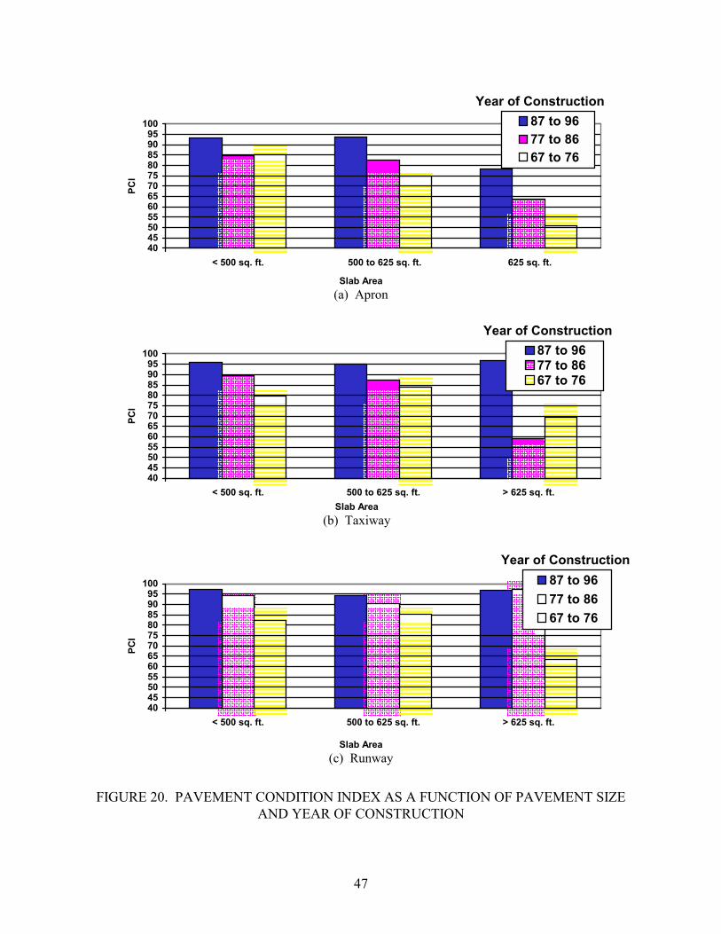
Year of Construction

100 95 90 85 80 75 70 65 60 55 50 45 40

< 500 sq. ft. 500 to 625 sq. ft. 625 sq. ft.

��

��

��

��

��

��

87 to 96

77 to 86 �� 67 to 76

Slab Area

(a) Apron


100 95 90 85 80 75 70 65 60 55 50 45 40

< 500 sq. ft. 500 to 625 sq. ft. > 625 sq. ft.

��

��

��

��

��

��

87 to 96 �� 77 to 86 ��

67 to 76

Slab Area

(b) Taxiway


100 95 90 85 80 75 70 65 60 55 50 45 40

< 500 sq. ft. 500 to 625 sq. ft. > 625 sq. ft.

��

��

��

��

��

��

87 to 96

77 to 86 �� 67 to 76

Slab Area

(c) Runway

FIGURE 20. PAVEMENT CONDITION INDEX AS A FUNCTION OF PAVEMENT SIZE AND YEAR OF CONSTRUCTION

PC

I P

CI

PC

I

47

TABLE 15. DATA FOR FIGURE 19PAVEMENT CONDITION INDEX AS A FUNCTIONOF PAVEMENT SIZE AND AGE

Age

Slab Area (sq. ft.)

0 to 10 Years 11 to 20 Years 21 to 30 Years

PCIAVG

Area (msf) PCIAVG

Area (msf) PCIAVG

Area (msf)

Apron < 500 91.0 23.0 81.5 7.9 84.1 13.0 500 to 625 86.4 11.6 79.1 7.7 68.7 5.3 > 625 68.3 0.8 56.4 3.9 44.8 1.4

Taxiway < 500 94.1 20.8 83.7 11.6 83.1 8.3 500 to 625 89.9 12.8 83.3 21.0 72.1 6.6 > 625 95.9 (C,D) 0.23 76.0 0.5 66.0 1.4

Runway < 500 96.6 10.4 86.6 8.5 86.6 10.5 500 to 625 92.9 12.2 87.7 23.1 79.6 5.5 > 625 97.3 (A,B) 0.16 75.0 2.7 62.5 0.3

TABLE 16. DATA FOR FIGURE 20PAVEMENT CONDITION INDEX AS A FUNCTIONOF PAVEMENT SIZE AND YEAR OF CONSTRUCTION

Year Constructed

Slab Area (sq. ft.)

1987—1996 1977—1986 1967—1976

PCIAVG

Area (msf) PCIAVG

Area (msf) PCIAVG

Area (msf)

Apron < 500 93.4 16.0 84.9 11.3 85.1 8.7 500 to 625 93.5 5.8 82.4 9.6 74.8 2.0 > 625 78.4 0.09 63.9 2.4 50.7 3.4

Taxiway < 500 96.1 11.6 89.5 11.3 79.7 9.8 500 to 625 95.0 3.7 87.2 10.3 84.0 17.4 > 625 96.8 (C) 0.23 59.0 (D) 0.005 69.3 1.9

Runway < 500 97.5 6.9 94.3 5.9 82.4 11.3 500 to 625 94.3 2.8 90.4 14.8 87.9 16.2 > 625 97.0 (A) 0.03 97.4 (B) 0.13 73.6 3.0

48

The results presented in figures 19 and 20 may be summarized as follows:

• PCI values of pavements using 500- to 625-sq. ft. slabs (mainly 25 by 20 ft and 25 by 25 ft) are generally lower than or close to those using smaller slabs. However, PCIs of pavements using slabs greater than 625 sq. ft. are much lower than the others except for runways and taxiways marked by (A), (B), (C), and (D) in tables 15 and 16. These pavements were younger than 10 years when they were surveyed, or they were built after 1987.

• Since the FAA design standard [1] recommends a maximum joint spacing of 25 feet, very few pavements having a slab size exceeding 25 by 25 feet have been built in the past 20 years. Table 17 lists all features in this study with slabs larger than 625 sq. ft. that are under 10 years old. As seen from table 17, only seven such features were identified. Also, in a number of cases, the slab size is only slightly larger than 625 sq. ft. In light of these considerations, it was felt that the amount of available data on newer slabs larger than 625 sq. ft. (indicated by notations (A), (B), (C), and (D) in tables 15 and 16) is not sufficient for a reliable statistical analysis of the performance of these slabs. If these data are excluded, then tables 15 and 16 show that the performance of slabs larger than the threshold 25 by 25 feet is significantly worse than the other slabs meeting FAA slab size criteria. On this basis, the FAA criteria appears to be justified.

• Figure 19 and table 15 indicate that the PCI of all pavements with slab size between 500 and 625 sq. ft. are generally lower than those with slab size smaller than 500 sq. ft. However, the differences are not significant if the pavements are less than 20 years old (i.e., within the design life).

• It can been seen from the same table and figure that the effects of slab size on PCI for older pavements (between 21 to 30 years) are much greater. Specifically, the larger slabs did not perform as well as the smaller slabs for older pavements (20 to 30 years old). This difference is especially apparent for apron pavements.

• Some of the data in table 16 and figure 20 apparently contradict the findings from table 15 and figure 19. This discrepancy is explained by the fact that most of the pavements built between 1967 and 1976 were younger than 20 years old at the time of inspection. (The pavement age is taken as the difference between the inspection year and the year of construction.) For example, many pavements having slab sizes in the 500- to 625-sq. ft. range that were in the 11- to 20-year age group in table 15 and figure 19 have been shifted into the 1967 to 1976 group in table 16 and figure 20. From the results presented, it is believed that the age of the pavement is a more suitable variable than the year of construction for analyzing the effects of slab size on PCI.

49

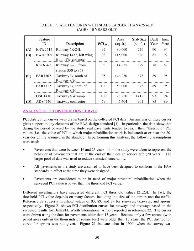
TABLE 17. ALL FEATURES WITH SLABS LARGER THAN 625 sq. ft. (AGE < 10 YEARS OLD)

Feature ID Description PCIAVG

Area (sq. ft.)

Slab Size (sq. ft.)

Built Year

Insp. Year

(A) ENW2515

(B) FWA6205

RST6340

(C) FAR1307

FAR1312

OSH1410

(D) ADS4740

Runway 6R/24L

Runway 1432, left wing from NW entrance

Runway 2-20, from

station 350 to 353

Taxiway B, south of Runway 8/26

Taxiway B, north of Runway 8/26

Taxiway SW ramp

Taxiway connector

97

98

93

95

100

100

59

30,600

115,000

14,855

146,250

53,000

28,250

5,404

729

626

629

675

675

1412

901

90

85

78

89

89

93

85

94

92

87

95

95

94

89

ANALYSIS OF PCI DISTRIBUTION CURVES.

PCI distribution curves were drawn based on the collected PCI data. An analysis of these curves gives support to key elements of the FAA design standard [1]. In particular, the data show that during the period covered by the study, real pavements tended to reach their “threshold” PCI values (i.e., the value of PCI at which major rehabilitation work is indicated) at or near the 20-year design life assumed in the standard. In performing this analysis, the following assumptions were used:

• Pavements that were between 16 and 23 years old in the study were taken to represent the behavior of pavements that are at the end of their design service life (20 years). The larger pool of data was used to reduce statistical uncertainty.

• All pavements in the study are assumed to have been designed to conform to the FAA standards in effect at the time they were designed.

• Pavements are considered to be in need of major structural rehabilitation when the surveyed PCI value is lower than the threshold PCI value.

Different investigators have suggested different PCI threshold values [21,23]. In fact, the threshold PCI value depends on many factors, including the size of the airport and the traffic. Reference 22 suggests threshold values of 93, 89, and 89 for runways, taxiways, and aprons, respectively. Figure 21 shows PCI distribution curves for runways and taxiways based on the surveyed results for Dallas/Ft. Worth International Airport reported in reference 22. The curves were drawn using the data for pavements older than 15 years. Because only a few aprons (with paved areas only in the thousands of square feet) were older than 15 years, the PCI distribution curve for aprons was not given. Figure 21 indicates that in 1990, when the survey was

50

conducted, approximately 94% of runway areas had PCI values higher than their threshold value (93), but only 55% of taxiway areas had PCI values higher than the suggested typical value of 89. However, the threshold values suggested in reference 22 are relatively high. More typical values used in practice by airports might be 80, 75, and 70 for runways, taxiways, and aprons, respectively.

Figure 22 illustrates PCI distribution curves for all surveyed pavements in the present study between 16 and 23 years old. Separate curves were drawn for runways, taxiways, and aprons. The survey data were obtained from 174 airports ranging from large hubs to regional airports. If 80, 75, and 70 are used as the respective threshold PCI values for runways, taxiways, and aprons, then according to figure 22, 80% of surveyed runways, 75% of surveyed taxiways, and 60% of the surveyed aprons had a surveyed PCI higher than the appropriate threshold values near the end of their design life.

PCI distribution data were also used to investigate the effects of slab size on the PCI for different functional categories of airport pavements. Figure 23 compares slab size effects on the PCI distribution for (a) aprons, (b) taxiways, and (c) runways. As in figure 22, the PCI distribution curves in figure 23 are based on pavements in the study between 16 and 23 years old. Pavements in this age group were divided into two groups according to their minimum slab side length. The two subgroups, (S1 + S2) and (S3 + S4), were previously defined in table 12 and figure 18.

100

90

80

70

60

50

40

30

20

10

0

50 55 60 65 70 75 80 85 90 95 100 105 PCI

Taxiway

Runway

FIGURE 21. PAVEMENT CONDITION INDEX DISTRIBUTION CURVE FOR DALLAS/FT. WORTH INTERNATIONAL AIRPORT

Per

cen

t o

f P

avem

ents

51

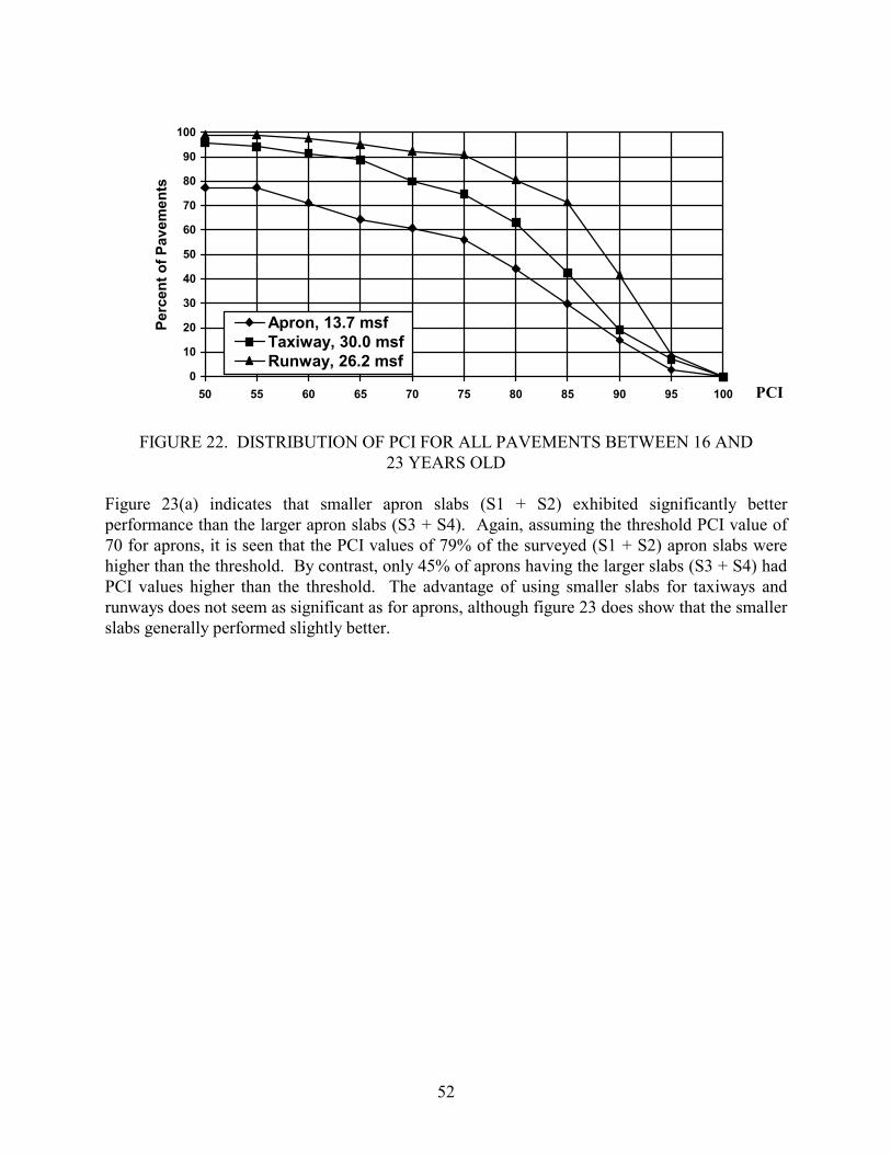
100

90

80

70

60

50

40

30

20

10

0

50 55 60 65 70 75 80 85 90 95 100 PCI

Apron, 13.7 msf Taxiway, 30.0 msf Runway, 26.2 msf

FIGURE 22. DISTRIBUTION OF PCI FOR ALL PAVEMENTS BETWEEN 16 AND 23 YEARS OLD

Figure 23(a) indicates that smaller apron slabs (S1 + S2) exhibited significantly better performance than the larger apron slabs (S3 + S4). Again, assuming the threshold PCI value of 70 for aprons, it is seen that the PCI values of 79% of the surveyed (S1 + S2) apron slabs were higher than the threshold. By contrast, only 45% of aprons having the larger slabs (S3 + S4) had PCI values higher than the threshold. The advantage of using smaller slabs for taxiways and runways does not seem as significant as for aprons, although figure 23 does show that the smaller slabs generally performed slightly better.

Per

cen

t o

f P

avem

ents

52

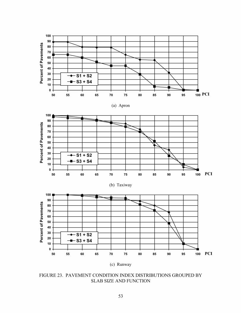
Per

cen

t o

f P

avem

ents

P

erce

nt

of

Pav

emen

tsP

erce

nt

of

Pav

emen

ts

100

90

80

70

60

50

40

30

20

10

0

100

90

80

70

60

50

40

30

20

10

0

100

90

80

70

60

50

40

30

20

10

0

S1 + S2 S3 + S4

50 55 60 65 70 75 80 85 90 95 100 PCI

(a) Apron

S1 + S2 S3 + S4

50 55 60 65 70 75 80 85 90 95 100 PCI

(b) Taxiway

S1 + S2 S3 + S4

50 55 60 65 70 75 80 85 90 95 100 PCI

(c) Runway

FIGURE 23. PAVEMENT CONDITION INDEX DISTRIBUTIONS GROUPED BY SLAB SIZE AND FUNCTION

53

CASE STUDY OF FOURTEEN AIRPORTS.

Performance of pavements is influenced not only by slab size but also by many other factors including: quality of original design and construction, traffic patterns, environmental factors, and routine maintenance procedures (such as joint sealing that if not performed results in premature distress). As shown in previous sections, pavements constructed with slabs larger than 625 sq. ft. generally give significantly worse performance than those constructed with smaller slab. For this reason, and because the current FAA design standard [1] explicitly recommends against using slabs larger than 25 by 25 feet, the following case study concentrates on comparing the performance of two groups of pavements: those with slabs smaller than 500 sq. ft. (group 1) and those with slabs in the range 500 to 625 sq. ft. Slabs exceeding 625 sq. ft. were excluded from consideration.

From the database of surveyed pavement data, all sets of data satisfying the following conditions were selected:

• Slabs from both groups that are used in the same airport and that are both used in at least one functional area (the two groups of slabs are used for aprons, taxiways, and runways).

• The total area in any group must have at least 200 slabs.

• The difference in the average age of the pavements in the two groups to be compared must be less than 2 years.

The average PCI of the pavements in the two groups was calculated. Since by assumption, the two groups of pavements are located at the same airport, the effects of environment on the pavement performance should be the same. Since the entire airport was managed by one organization, the differences in maintenance management would be negligible. The average ages of the two groups of pavements are less than 2 years, so the effects of pavement age on the performance do not need to be considered. Therefore, comparison of PCI values for the two groups is a good indicator of the slab size effects on the pavement performance.

Table 18 lists data for apron pavements at eight airports. For each slab size category, the average size, age, and PCI are listed. Similar data are given in tables 19 and 20 for taxiways and runways respectively. Table 21 compares slab size effects for aprons, taxiways, and runways. A significant difference between groups, either better or worse, is defined as a difference of two points in the average PCI. If the difference in PCI is less than two points, the performances of the two groups are considered to be similar.

The performances of pavements using smaller slabs were generally better than those using larger slabs. The results verify the findings arrived at previously by general statistical analysis.

54

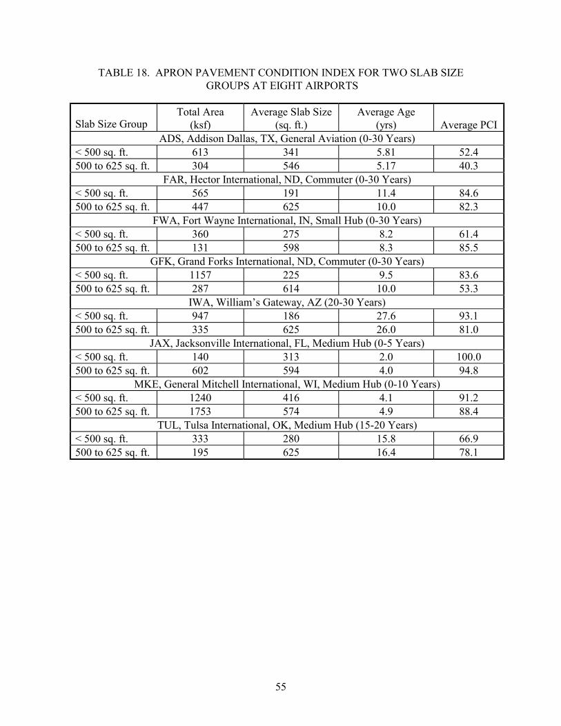
TABLE 18. APRON PAVEMENT CONDITION INDEX FOR TWO SLAB SIZEGROUPS AT EIGHT AIRPORTS

Slab Size Group Total Area

(ksf) Average Slab Size

(sq. ft.) Average Age

(yrs) Average PCI ADS, Addison Dallas, TX, General Aviation (0-30 Years)

< 500 sq. ft. 613 341 5.81 52.4 500 to 625 sq. ft. 304 546 5.17 40.3

FAR, Hector International, ND, Commuter (0-30 Years) < 500 sq. ft. 565 191 11.4 84.6 500 to 625 sq. ft. 447 625 10.0 82.3

FWA, Fort Wayne International, IN, Small Hub (0-30 Years) < 500 sq. ft. 360 275 8.2 61.4 500 to 625 sq. ft. 131 598 8.3 85.5

GFK, Grand Forks International, ND, Commuter (0-30 Years) < 500 sq. ft. 1157 225 9.5 83.6 500 to 625 sq. ft. 287 614 10.0 53.3

IWA, William’s Gateway, AZ (20-30 Years) < 500 sq. ft. 947 186 27.6 93.1 500 to 625 sq. ft. 335 625 26.0 81.0

JAX, Jacksonville International, FL, Medium Hub (0-5 Years) < 500 sq. ft. 140 313 2.0 100.0 500 to 625 sq. ft. 602 594 4.0 94.8

MKE, General Mitchell International, WI, Medium Hub (0-10 Years) < 500 sq. ft. 1240 416 4.1 91.2 500 to 625 sq. ft. 1753 574 4.9 88.4

TUL, Tulsa International, OK, Medium Hub (15-20 Years) < 500 sq. ft. 333 280 15.8 66.9 500 to 625 sq. ft. 195 625 16.4 78.1

55

TABLE 19. TAXIWAY PAVEMENT CONDITION INDEX FOR TWO SLAB SIZE GROUPSAT EIGHT AIRPORTS




(yrs) Average PCI

CWA, Central Wisconsin, WI, Commuter (15-25 Years) < 500 sq. ft. 820 246 20.0 66.1 500 to 625 sq. ft. 190 529 18.4 44.3

FAR, Hector International, ND, Commuter (0-30 Years) < 500 sq. ft. 776 372 17.0 75.5 500 to 625 sq. ft. 1244 614 18.4 75.5

IWA, William’s Gateway, AZ, N/A (0-5 Years) < 500 sq. ft. 114 200 4.3 95.6 500 to 625 sq. ft. 150 547 3.0 96.3

MKE, General Mitchell International, WI, Medium Hub (0-30 Years) < 500 sq. ft. 2270 360 15.0 77.8 500 to 625 sq. ft. 1206 509 15.7 75.6

OSH, Wittman Regional, WI, Commuter (10-30 Years) < 500 sq. ft. 1352 250 22.6 84.8 500 to 625 sq. ft. 181 597 17.0 76.0

RDU, Raleigh-Durham International, NC, Medium (6-10 Years) < 500 sq. ft. 339 312.5 8.0 94.7 500 to 625 sq. ft. 131 625 8.0 89.6

RHI, Rhinelander-Oneida County, NY (5-10 Years) < 500 sq. ft. 119 441 8.0 72.9 500 to 625 sq. ft. 367 622 8.0 76.0

TUL, Tulsa International, OK, Medium Hub (0-30 Years) < 500 sq. ft. 3725 398 12.6 85.5 500 to 625 sq. ft. 1350 605 11.7 85.1

TABLE 20. RUNWAY PAVEMENT CONDITION INDEX FOR TWO SLAB SIZE GROUPSAT THREE AIRPORTS




(yrs) Average PCI FAR, Hector International, ND, Commuter (20-30 Years)

< 500 sq. ft. 1456 269 25.0 75.9 500 to 625 sq. ft. 540 625 25.4 67.6

MKE, General Mitchell International, WI, Medium Hub (25-30 Years) < 500 sq. ft. 268 302 26.7 70.3 500 to 625 sq. ft. 406 505 26 61.8

TUL, Tulsa International, OK, Medium Hub (10-15 Years) < 500 sq. ft. 284 158 12 91.7 500 to 625 sq. ft. 1717 623 12 89.6

56

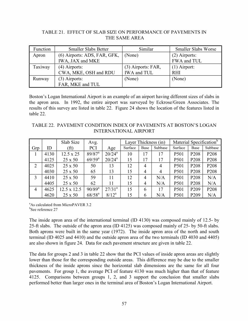
TABLE 21. EFFECT OF SLAB SIZE ON PERFORMANCE OF PAVEMENTS INTHE SAME AREA

Function Smaller Slabs Better Similar Smaller Slabs Worse Apron (6) Airports: ADS, FAR, GFK,

IWA, JAX and MKE (None) (2) Airports:

FWA and TUL Taxiway (4) Airports:

CWA, MKE, OSH and RDU (3) Airports: FAR, IWA and TUL

(1) Airport: RHI

Runway (3) Airports: FAR, MKE and TUL

(None) (None)

Boston’s Logan International Airport is an example of an airport having different sizes of slabs in the apron area. In 1992, the entire airport was surveyed by Eckrose/Green Associates. The results of this survey are listed in table 22. Figure 24 shows the location of the features listed in table 22.

TABLE 22. PAVEMENT CONDITION INDEX OF PAVEMENTS AT BOSTON’S LOGAN INTERNATIONAL AIRPORT

Grp ID Slab Size

(ft) Avg. PCI Age

Layer Thickness (in) Material Specification b

Surface Base Subbase Surface Base Subbase

1 4130 4125

12.5 x 25 25 x 50

89/87a

69/59a 20/24a

20/24a 10 15

17 17

17 17

P501 P501

P208 P208

P208 P208

2 4025 4030

25 x 50 25 x 50

50 65

13 13

12 15

4 4

4 4

P501 P501

P208 P208

P208 P208

3 4410 4405

25 x 50 25 x 50

59 62

11 11

12 15

4 4

N/A N/A

P501 P501

P208 P208

N/A N/A

4 4625 4620

12.5 x 12.5 25 x 50

90/89a

68/58a 27/31a

8/12a 15 15

6 6

17 N/A

P501 P501

P209 P209

P208 N/A

aAs calculated from MicroPAVER 3.2 bSee reference 27

The inside apron area of the international terminal (ID 4130) was composed mainly of 12.5- by 25-ft slabs. The outside of the apron area (ID 4125) was composed mainly of 25- by 50-ft slabs. Both aprons were built in the same year (1972). The inside apron area of the north and south terminal (ID 4025 and 4410) and the outside apron area of the two terminals (ID 4030 and 4405) are also shown in figure 24. Data for each pavement structure are given in table 22.

The data for groups 2 and 3 in table 22 show that the PCI values of inside apron areas are slightly lower than those for the corresponding outside areas. This difference may be due to the smaller thickness of the inside aprons since the horizontal slab dimensions are the same for all four pavements. For group 1, the average PCI of feature 4130 was much higher than that of feature 4125. Comparisons between groups 1, 2, and 3 support the conclusion that smaller slabs performed better than larger ones in the terminal area of Boston’s Logan International Airport.

57

FIGURE 24. TERMINAL AREA OF BOSTON’S LOGAN INTERNATIONAL AIRPORT

The two areas listed in group 4 in table 22 are holding areas for aircraft temporarily being pulled from the terminal gates. These two areas are not far from each other and have similar pavement structures. Table 22 shows that feature 4625 had a PCI much higher than feature 4620, though the former was much older. Higher PCI values seem to be associated with smaller slab sizes.

In table 22, where two values of PCI appear for a feature, the first value was surveyed by Eckrose/Green Associates in 1992. Features 4130, 4125, 4625, and 4530 were resurveyed in May 1996 with the assistance of the Boston’s Logan International Airport Pavement Maintenance Team. The second value listed in column 4 of table 22 (groups 1 and 4) was calculated using MicroPaver 3.2. One hundred percent samples were used in this second survey, rather than a representative portion of the pavement as was used by Eckrose/Green Associates in 1992.

The results of the two surveys are consistent with each other. It is interesting to note that after 4 years the PCI of small slabs (12.5 by 25 ft and 12.5 by 12.5 ft) dropped 1 to 2 points while the PCI of larger slabs (25 by 50 ft) dropped about 10 points. The comparison of surveyed data verifies again that the 25- by 50-ft slabs performed more poorly than smaller slabs.

58

It should also be pointed out that the apron pavements at Boston’s Logan International Airport have been well maintained for many years. Seal damage was seldom observed and almost all sealing material remained elastic when the survey was conducted in 1996. The major PCI reduction was caused by cracks. The majority of the 25- by 50-ft slabs were cracked into two or three pieces even though the California bearing ratio (CBR) of the subgrade was expected to be higher than 20 in that area.

CONCLUSIONS

Pavement performance is influenced by many factors: original pavement design, material techniques used in construction, actual aircraft traffic mixture, environmental effects, routine maintenance procedures, pavement age, etc. Slab size, which is determined by joint spacing, is only one of the design variables influencing the pavement performance. It is common in a pavement survey to find that some pavements using smaller slabs perform better than those using larger slabs while in other pavements the larger slabs perform better. It is important to separate the effects of slab size from other effects mixed together to appropriately evaluate the effect of the slab size on pavement performance under realistic conditions in airports throughout the U.S.

Although it is impossible in a field investigation to isolate the slab size effect completely, it is possible nevertheless to minimize the effects of other factors by careful consideration of all available relevant data. The present investigation focused on the slab size effect but also considered many other variables that can affect performance. By examining the relative performance of groups of pavement features that are alike in other respects but that have different slab dimensions, the important influence of slab size in particular was demonstrated.

The effect of slab size on pavement performance was evaluated by investigating the effects on the maximum bending stress at the pavement joint. The effect of slab size on the maximum bending stress is not equivalent to the effect of slab size on pavement performance. However, the two effects are closely related and examining one provides insight to the other.

Two initial states and two types of responses were considered to evaluate the effect of slab size on the maximum bending stress at pavement joints. The two initial states were (1) the surface slabs maintain full contact with the base or subbase layer (in other words, the initial warping and curling of the slabs caused by temperature gradient and other environmental loads is not considered) and (2) the surface slabs are warped up or curled down by a temperature gradient such that gaps exist between the surface slabs and the base or subbase layer. The two response types were (1) responses induced by vehicular load only and (2) the total responses induced by both the vehicular load and the temperature gradient. Different initial states and response types may have led to different conclusions about the effect of the slab size on the pavement response. Specific conclusions of this study are

• Numerical analysis, using the finite element method for cases having different slab widths under representative gear loads, show that the slab width has an insignificant effect on load-induced responses (type 1) regardless of the initial states 1 or 2, but it has a significant effect on the total stress-induced responses (including both vehicle load and

59

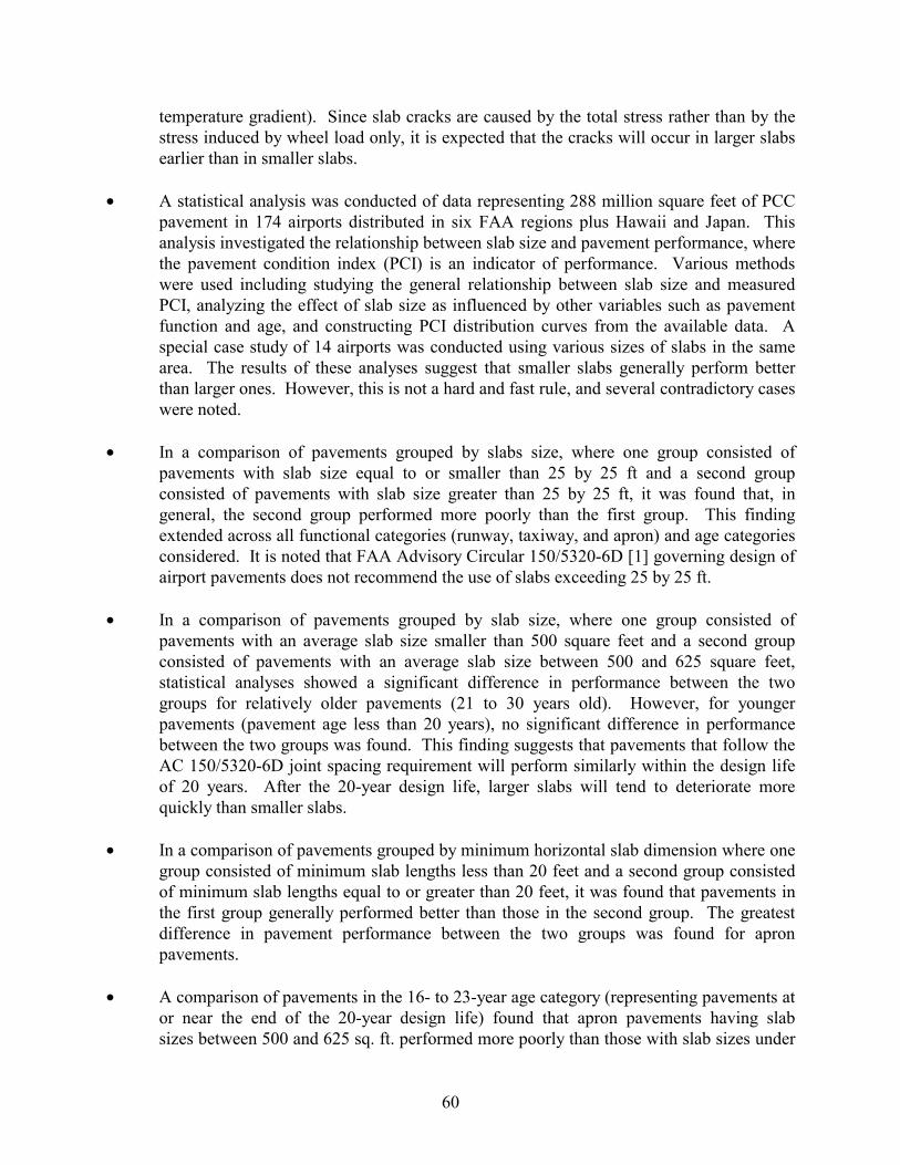
temperature gradient). Since slab cracks are caused by the total stress rather than by the stress induced by wheel load only, it is expected that the cracks will occur in larger slabs earlier than in smaller slabs.

• A statistical analysis was conducted of data representing 288 million square feet of PCC pavement in 174 airports distributed in six FAA regions plus Hawaii and Japan. This analysis investigated the relationship between slab size and pavement performance, where the pavement condition index (PCI) is an indicator of performance. Various methods were used including studying the general relationship between slab size and measured PCI, analyzing the effect of slab size as influenced by other variables such as pavement function and age, and constructing PCI distribution curves from the available data. A special case study of 14 airports was conducted using various sizes of slabs in the same area. The results of these analyses suggest that smaller slabs generally perform better than larger ones. However, this is not a hard and fast rule, and several contradictory cases were noted.

• In a comparison of pavements grouped by slabs size, where one group consisted of pavements with slab size equal to or smaller than 25 by 25 ft and a second group consisted of pavements with slab size greater than 25 by 25 ft, it was found that, in general, the second group performed more poorly than the first group. This finding extended across all functional categories (runway, taxiway, and apron) and age categories considered. It is noted that FAA Advisory Circular 150/5320-6D [1] governing design of airport pavements does not recommend the use of slabs exceeding 25 by 25 ft.

• In a comparison of pavements grouped by slab size, where one group consisted of pavements with an average slab size smaller than 500 square feet and a second group consisted of pavements with an average slab size between 500 and 625 square feet, statistical analyses showed a significant difference in performance between the two groups for relatively older pavements (21 to 30 years old). However, for younger pavements (pavement age less than 20 years), no significant difference in performance between the two groups was found. This finding suggests that pavements that follow the AC 150/5320-6D joint spacing requirement will perform similarly within the design life of 20 years. After the 20-year design life, larger slabs will tend to deteriorate more quickly than smaller slabs.

• In a comparison of pavements grouped by minimum horizontal slab dimension where one group consisted of minimum slab lengths less than 20 feet and a second group consisted of minimum slab lengths equal to or greater than 20 feet, it was found that pavements in the first group generally performed better than those in the second group. The greatest difference in pavement performance between the two groups was found for apron pavements.

• A comparison of pavements in the 16- to 23-year age category (representing pavements at or near the end of the 20-year design life) found that apron pavements having slab sizes between 500 and 625 sq. ft. performed more poorly than those with slab sizes under

60

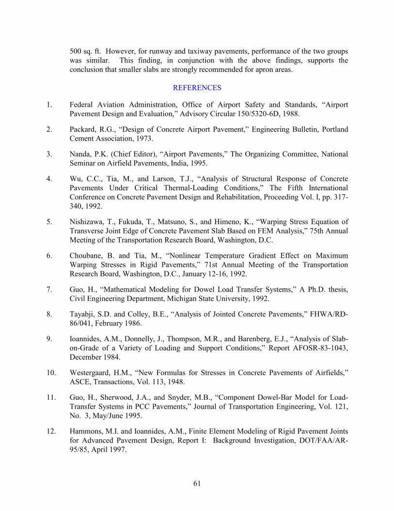
500 sq. ft. However, for runway and taxiway pavements, performance of the two groups was similar. This finding, in conjunction with the above findings, supports the conclusion that smaller slabs are strongly recommended for apron areas.

REFERENCES

1. Federal Aviation Administration, Office of Airport Safety and Standards, “Airport Pavement Design and Evaluation,” Advisory Circular 150/5320-6D, 1988.

2. Packard, R.G., “Design of Concrete Airport Pavement,” Engineering Bulletin, Portland Cement Association, 1973.

3. Nanda, P.K. (Chief Editor), “Airport Pavements,” The Organizing Committee, National Seminar on Airfield Pavements, India, 1995.

4. Wu, C.C., Tia, M., and Larson, T.J., “Analysis of Structural Response of Concrete Pavements Under Critical Thermal-Loading Conditions,” The Fifth International Conference on Concrete Pavement Design and Rehabilitation, Proceeding Vol. I, pp. 317-340, 1992.

5. Nishizawa, T., Fukuda, T., Matsuno, S., and Himeno, K., “Warping Stress Equation of Transverse Joint Edge of Concrete Pavement Slab Based on FEM Analysis,” 75th Annual Meeting of the Transportation Research Board, Washington, D.C.

6. Choubane, B. and Tia, M., “Nonlinear Temperature Gradient Effect on Maximum Warping Stresses in Rigid Pavements,” 71st Annual Meeting of the Transportation Research Board, Washington, D.C., January 12-16, 1992.

7. Guo, H., “Mathematical Modeling for Dowel Load Transfer Systems,” A Ph.D. thesis, Civil Engineering Department, Michigan State University, 1992.

8. Tayabji, S.D. and Colley, B.E., “Analysis of Jointed Concrete Pavements,” FHWA/RD-86/041, February 1986.

9. Ioannides, A.M., Donnelly, J., Thompson, M.R., and Barenberg, E.J., “Analysis of Slab-on-Grade of a Variety of Loading and Support Conditions,” Report AFOSR-83-1043, December 1984.

10. Westergaard, H.M., “New Formulas for Stresses in Concrete Pavements of Airfields,” ASCE, Transactions, Vol. 113, 1948.

11. Guo, H., Sherwood, J.A., and Snyder, M.B., “Component Dowel-Bar Model for Load-Transfer Systems in PCC Pavements,” Journal of Transportation Engineering, Vol. 121, No. 3, May/June 1995.

12. Hammons, M.I. and Ioannides, A.M., Finite Element Modeling of Rigid Pavement Joints for Advanced Pavement Design, Report I: Background Investigation, DOT/FAA/AR-95/85, April 1997.

61

13. Bradbury, R.D., “Reinforced Concrete Pavements,” Wire Institute, Washington, DC, 1938 cited by Yoder, E.J. and Witczak, M.W., “Principles of Pavement Design,” John Wiley and Sons, Inc., 1975.

14. Nilson, A.H., “Design of Concrete Structures,” McGraw Hill, Inc., 1991.

15. Armaghani, “Factors Affecting Performance of Concrete Pavements,” The Fifth International Conference on Concrete Pavement Design and Rehabilitation, Proceeding Vol. I, pp. 33-46, 1993.

16. Federal Aviation Administration, Office of Airport Safety and Standards, “Airport Pavement Design for the Boeing 777 Airplane,” Advisory Circular 150/5320-16, 1995.

17. FAA, Office of Airport Safety and Standards, “Guidelines and Procedures for Maintenance of Airport Pavements,” Advisory Circular 150/5380-6, December 1982.

18. FAA, Airport Safety Data Branch, “Airport Safety Data Program, Order 5010.4,” Initiated in January 1981, database updated in 1995.

19. Kurtz, Max, “Handbook of Applied Mathematics for Engineers and Scientists,” McGraw Hill, 1991.

20. Eckrose/Green Associates, Inc., “Airport Pavement Inspection by PCI,” Survey Handbook, 1996.

21. Eckrose/Green Associates, Inc., “Airport Pavement Evaluation,” Logan International Airport, Boston, MA, 1992.

22. Harding Lawson Associates, Pavement Consulting Inc., and Surface Dynamics Inc., “Dallas/Fort Worth International Airport Pavement Management Consulting Services, Final Report, March 1992.

23. McQueen, R.D., “Evaluation of Runway and Taxiway Pavements at Atlantic City International Airport, Atlantic City, NJ,” June 1995.

24. McQueen, R.D., “Evaluation of Airfield Pavements at Cincinnati/Northern Kentucky International Airport,” Engineering Report for Survey Results, February 1993.

25. McQueen, R.D., “Evaluation of Runway 10C-28C and Taxiway W Pavements at Greater Pittsburgh International Airport, PA,” October 1991.

26. ERES Consultants, Inc., “Evaluation of the Airside Pavement at Raleigh-Durham International Airport, Morrisville, North Carolina,” March 1995.

27. Federal Aviation Administration, Office of Airport Safety and Standards, “Standard for Specifying Construction of Airports,” Advisory Circular 150/5370-10A, 1991.

62

A-1

APPENDIX A COMPUTATIONAL RESULTS

0 100 200 300 400 500 600 7000

50

100

150

200

250

300

350

400

450

(a) (Intended to illustrate the shape of the lines of constant response only; units are in inches.)

0

200

400

600

0

100

200

300

400

-0.04

-0.02

0

0.02

inch

es

(b) Three-Dimensional View (Units are in inches.)

FIGURE A-1. ACE DEFLECTIONS DUE TO B-727 EDGE LOAD, g = 0

Contour View

SURF

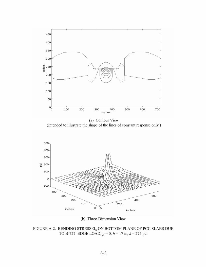
A-2

0 100 200 300 400 500 600 7000

50

100

150

200

250

300

350

400

450

inches

inch

es

(a) (Intended to illustrate the shape of the lines of constant response only.)

0

200

400

600

0

100

200

300

400

-100

0

100

200

300

400

500

inchesinches

psi

(b)

FIGURE A-2. NG STRESS σx ON BOTTOM PLANE OF PCC SLABS DUETO B-727 OAD, g = 0, h = 17 in, k = 275 pci

Contour View

Three-Dimension View

BENDIEDGE L

A-3

0 100 200 300 400 500 600 7000

50

100

150

200

250

300

350

400

450


0

200

400

600

0

100

200

300

400

-0.04

-0.02

0

0.02

inch

es


FIGURE A-3. URFACE DEFLECTIONS DUE TO DC-10-10 EDGE LOAD, g = 0

Contour View

S

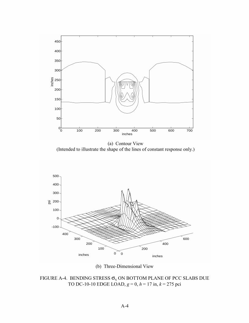
A-4

0 100 200 300 400 500 600 7000

50

100

150

200

250

300

350

400

450

inches

inch

es


0

200

400

600

0

100

200

300

400

-100

0

100

200

300

400

500

inchesinches

psi

(b)

FIGURE A-4. NG STRESS σx ON BOTTOM PLANE OF PCC SLABS DUETO DC-10-10 EDGE LOAD, g = 0, h = 17 in, k = 275 pci

Contour View

Three-Dimensional View

BENDI

A-5

0 100 200 300 400 500 600 7000

50

100

150

200

250

300

350

400

450


0

200

400

600

0

100

200

300

400

-0.04

-0.02

0

0.02

inch

es


FIGURE A-5. ACE DEFLECTIONS DUE TO B-777 EDGE LOAD, g = 0

Contour View

SURF

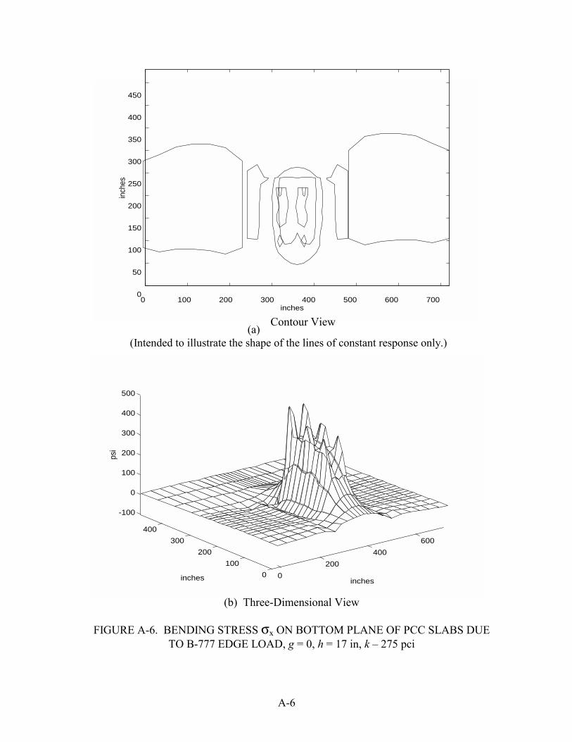
A-6

0 100 200 300 400 500 600 7000

50

100

150

200

250

300

350

400

450

inches

inch

es


0

200

400

600

0

100

200

300

400

-100

0

100

200

300

400

500

inchesinches

psi

(b)

FIGURE A-6. NG STRESS σx ON BOTTOM PLANE OF PCC SLABS DUETO B-777 EDGE LOAD, g = 0, h = 17 in, k – 275 pci

Contour View


BENDI

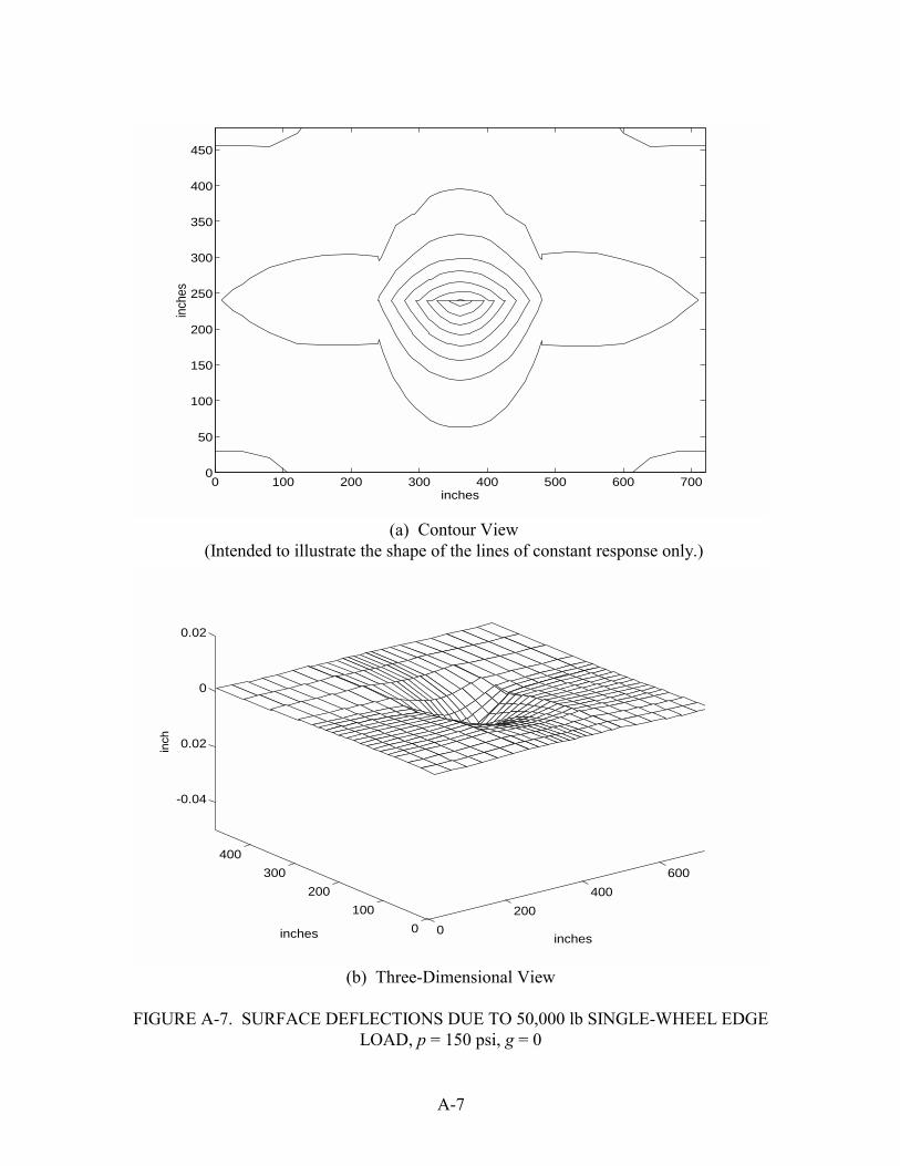
A-7

0 100 200 300 400 500 600 7000

50

100

150

200

250

300

350

400

450

inches

inch

es


0

200

400

600

0

100

200

300

400

-0.04

-0.02

0

0.02

inchesinches

inch

es

(b)

FIGURE A-7. ACE DEFLECTIONS DUE TO 50,000 lb SINGLE-WHEEL EDGELOAD, p = 150 psi, g = 0

inch

Contour View


SURF

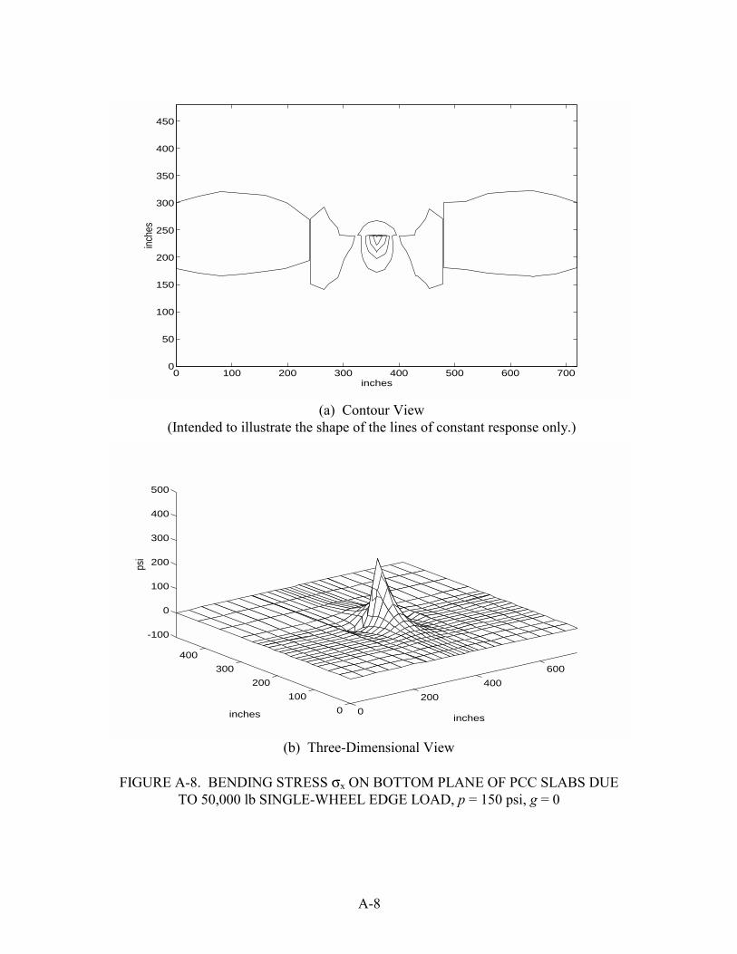
A-8

0 100 200 300 400 500 600 7000

50

100

150

200

250

300

350

400

450

inches

inch

es


0

200

400

600

0

100

200

300

400

-100

0

100

200

300

400

500

inchesinches

psi

(b)

FIGURE A-8. NG STRESS σx ON BOTTOM PLANE OF PCC SLABS DUETO 50,000 lb SINGLE-WHEEL EDGE LOAD, p = 150 psi, g = 0

Contour View


BENDI

A-9

0

200

400

600

0

100

200

300

400

-0.04

-0.02

0

0.02

inchesinches

inch

es

(a) Nighttime Temperature Gradient g = -1.5°F/inch

0

200

400

600

0

100

200

300

400

-0.04

-0.02

0

0.02

inchesinches

inch

es

(b) Daytime Temperature Gradient g = 1.5°F/inch

FIGURE A-9. LECTIONS UNDER A B-727 LANDING GEAR LOAD BASEDON TEMPERATURE-INDUCED INITIAL PAVEMENT STATES

inch

inch

DEF

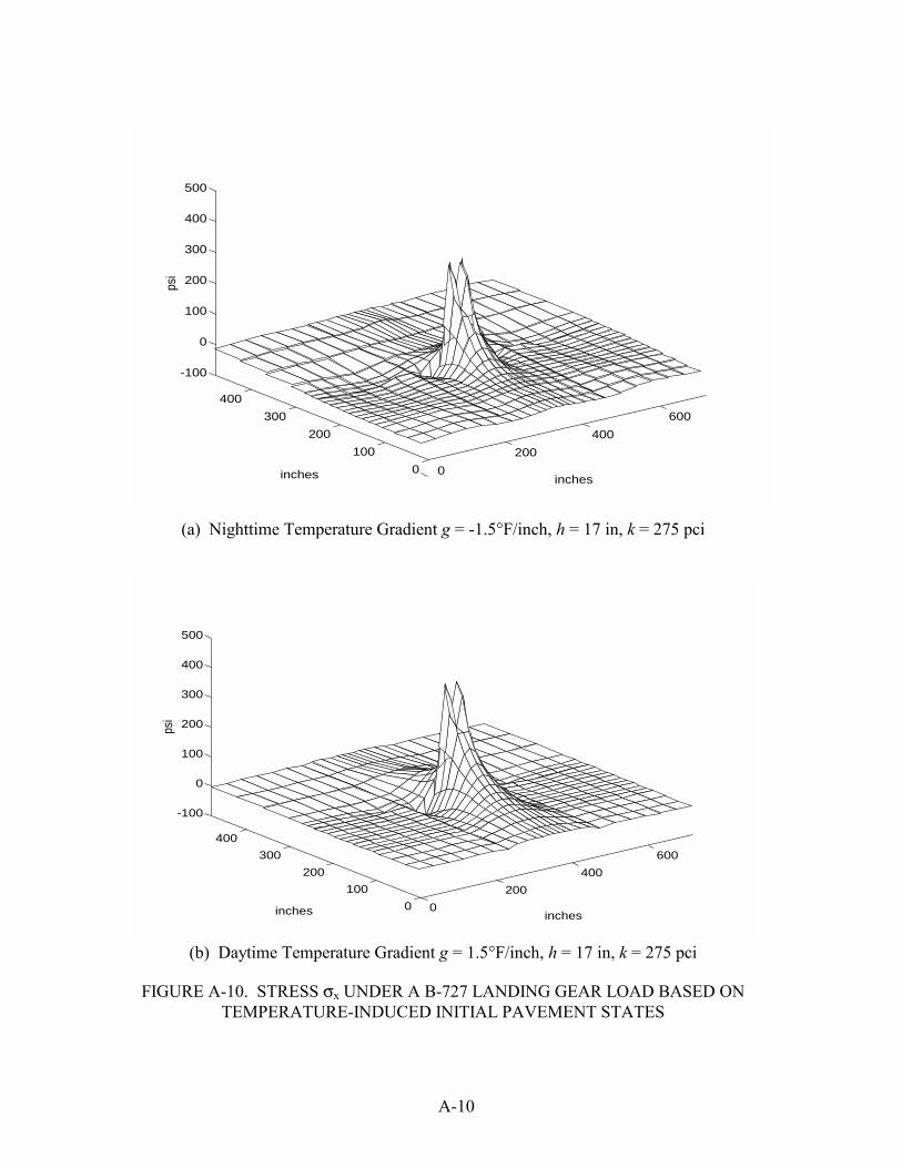
A-10

0

200

400

600

0

100

200

300

400

-100

0

100

200

300

400

500

inchesinches

psi

(a) Nighttime Temperature Gradient g = -1.5°F/inch, h = 17 in, k = 275 pci

0

200

400

600

0

100

200

300

400

-100

0

100

200

300

400

500

inchesinches

psi

(b) Daytime Temperature Gradient g = 1.5°F/inch, h = 17 in, k = 275 pci

FIGURE A-10. σx UNDER A B-727 LANDING GEAR LOAD BASED ONTEMPERATURE-INDUCED INITIAL PAVEMENT STATES

STRESS

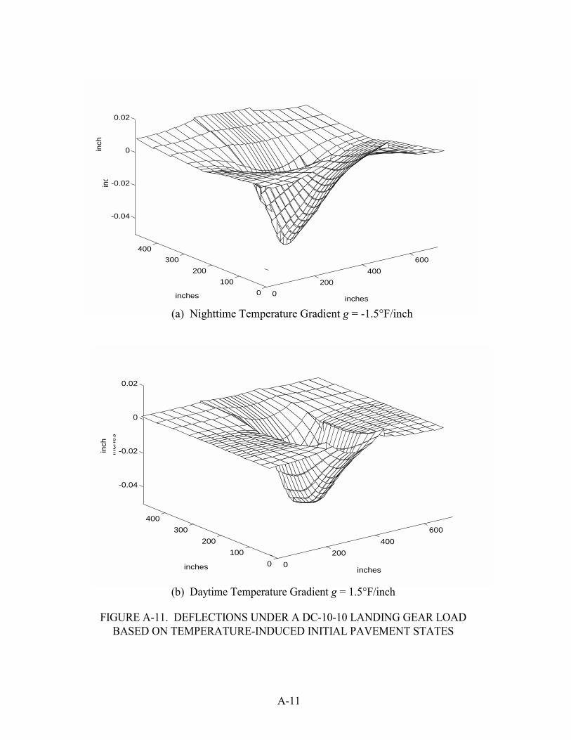
A-11

0

200

400

600

0

100

200

300

400

-0.04

-0.02

0

0.02

inchesinches

inch

es


0

200

400

600

0

100

200

300

400

-0.04

-0.02

0

0.02

inchesinches

inch

es


FIGURE A-11. LECTIONS UNDER A DC-10-10 LANDING GEAR LOADBASED ON TEMPERATURE-INDUCED INITIAL PAVEMENT STATES

inch

inch

DEF

A-12

0

200

400

600

0

100

200

300

400

-100

0

100

200

300

400

500

inchesinches

psi


0

200

400

600

0

100

200

300

400

-100

0

100

200

300

400

500

inchesinches

psi


FIGURE A-12. σx UNDER A DC-10-10 LANDING GEAR LOAD BASEDON TEMPERATURE-INDUCED INITIAL PAVEMENT STATES

STRESS

A-13

0

200

400

600

0

100

200

300

400

-0.04

-0.02

0

0.02

inchesinches

inch

es


0

200

400

600

0

100

200

300

400

-0.04

-0.02

0

0.02

inchesinches

inch

es


FIGURE A-13. LECTIONS UNDER A B-777 LANDING GEAR LOAD BASEDON TEMPERATURE-INDUCED INITIAL PAVEMENT STATES

inch

inch

DEF

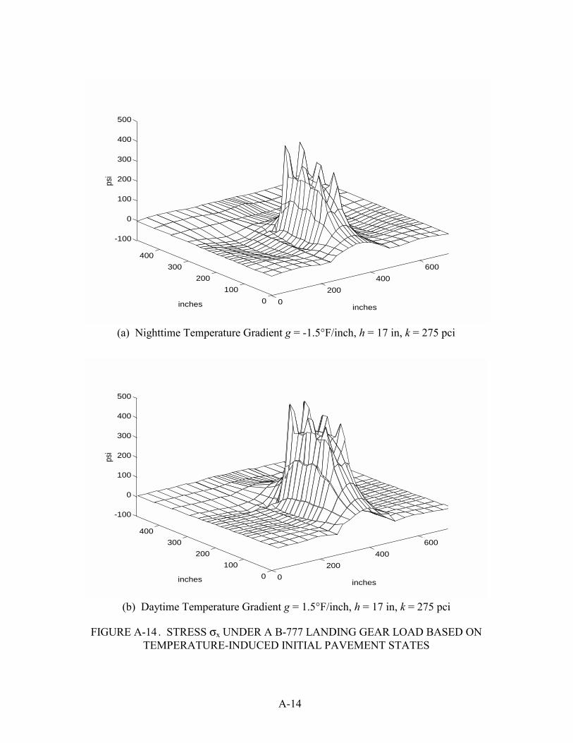
A-14

0

200

400

600

0

100

200

300

400

-100

0

100

200

300

400

500

inchesinches

psi


0

200

400

600

0

100

200

300

400

-100

0

100

200

300

400

500

inchesinches

psi


FIGURE A-14 . TRESS σx UNDER A B-777 LANDING GEAR LOAD BASED ONTEMPERATURE-INDUCED INITIAL PAVEMENT STATES

S

A-15

0

200

400

600

0

100

200

300

400

-0.04

-0.02

0

0.02

inchesinches

inch

es

(a) Nighttime Temperature Gradient g = -1.5°F/inch, p = 150 psi

0

200

400

600

0

100

200

300

400

-0.04

-0.02

0

0.02

inchesinches

inch

es

(b) Daytime Temperature Gradient g = 1.5°F/inch, p = 150 psi

FIGURE A-15. LECTIONS UNDER A 50,000 lb SINGLE-WHEEL LOADBASED ON TEMPERATURE-INDUCED INITIAL PAVEMENT STATES

inch

inch

DEF

A-16

0

200

400

600

0

100

200

300

400

-100

0

100

200

300

400

500

inchesinches

psi

(a) Nighttime Temperature Gradient g = -1.5°F/inch, p = 150 psi

0

200

400

600

0

100

200

300

400

-100

0

100

200

300

400

500

inchesinches

psi

(b) Daytime Temperature Gradient g = 1.5°F/inch, p = 150 psi

FIGURE A-16 . TRESS σx UNDER A 50,000 lb SINGLE-WHEEL LOAD BASED ONTEMPERATURE-INDUCED INITIAL PAVEMENT STATES

S

406080100

0

-0.01

-0.02

-0.03

-0.04

-0.05

-0.06

0 50 100 150 200 250 300 350 400

g = 0 g = -1.5

g = 1.5

Symmetric Axis

(a) -727 Landing Gear Under a B

0 50 100 150 200 250 300 350 400

0

-0.01

-0.02

-0.03

-0.04

-0.05

-0.06

g = 0 g = -1.5

g = 1.5

Symmetric Axis

(b) Under a DC-10-10 Landing Gear

0 50 100 150 200 250 300 350 400

0

-0.01

-0.02

-0.03

-0.04

-0.05

-0.06

-0.07

g = 0 g = -1.5

g = 1.5

Symmetric Axis

(c) Under a B-777 Landing Gear

(All units in inches)

FIGURE A-17. DEFLECTIONS AT THE JOINT (ON THE LOADED SIDE)

A-17

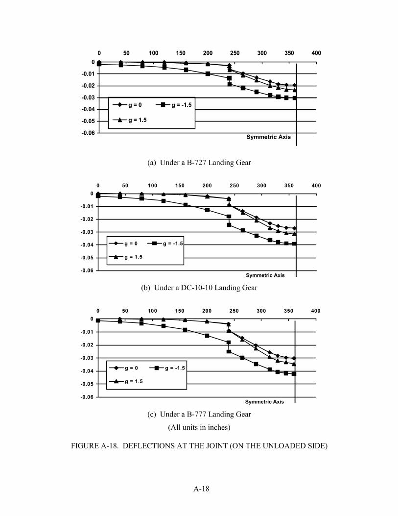
0 50 100 150 200 250 300 350 400

0

-0.01

-0.02

-0.03

-0.04

-0.05

-0.06

g = 0 g = -1.5

g = 1.5

Symmetric Axis

0

-0.01

-0.02

-0.03

-0.04

-0.05

-0.06

0

-0.01

-0.02

-0.03

-0.04

-0.05

-0.06

(a) Under a B-727 Landing Gear

0 50 100 150 200 250 300 350 400

g = 0 g = -1.5

g = 1.5

Symmetric Axis


0 50 100 150 200 250 300 350 400

g = 0 g = -1.5

g = 1.5

Symmetric Axis



FIGURE A-18. DEFLECTIONS AT THE JOINT (ON THE UNLOADED SIDE)

A-18

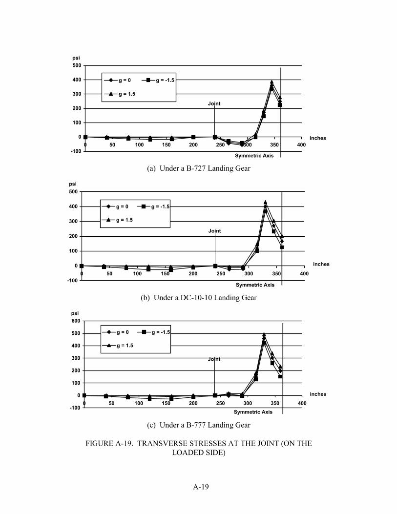
psi

500

400

300

200

100

0

0 50 100 150 200 250 300 350 400

g = 0 g = -1.5

g = 1.5

Symmetric Axis

Joint

inches

-100


psi

500

400

300

200

100

0

0 50 100 150 200 250 300 350 400

g = 0 g = -1.5

g = 1.5

Symmetric Axis

Joint

inches

-100

psi

600

500

400

300

200

100

0

-100


0 50 100 150 200 250 300 350 400

g = 0 g = -1.5

g = 1.5

Symmetric Axis

Joint

inches


FIGURE A-19. TRANSVERSE STRESSES AT THE JOINT (ON THE LOADED SIDE)

A-19

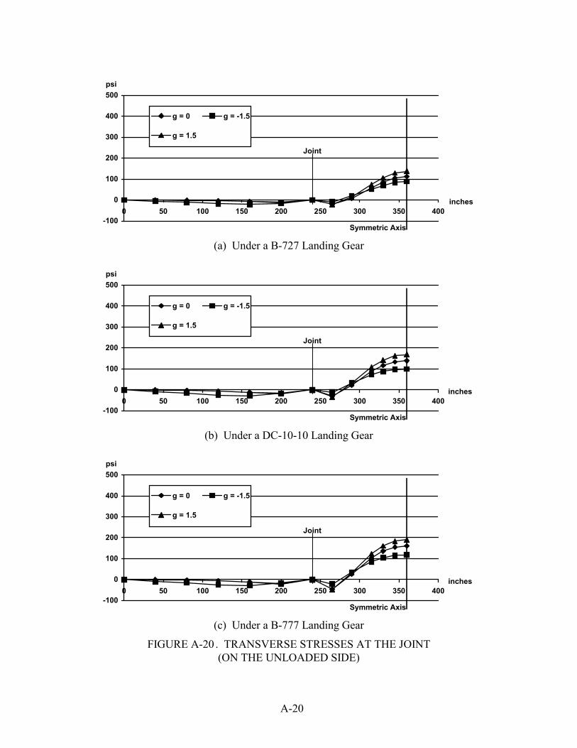
psi

500

400

300

200

100

0

0 50 100 150 200 250 300 350 400

g = 0 g = -1.5

g = 1.5

Symmetric Axis

Joint

inches

-100


psi

500

400

300

200

100

0

0 50 100 150 200 250 300 350 400

g = 0 g = -1.5

g = 1.5

Symmetric Axis

Joint

inches

-100


psi

500

400

300

200

100

0

0 50 100 150 200 250 300 350 400

g = 0 g = -1.5

g = 1.5

Symmetric Axis

Joint

inches

-100


FIGURE A-20 . TRANSVERSE STRESSES AT THE JOINT (ON THE UNLOADED SIDE)

A-20

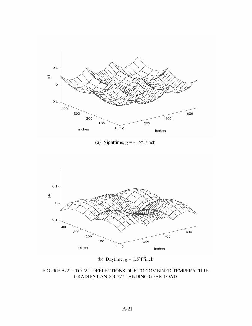
A-21

0

200

400

600

0

100

200

300

400

-0.1

0

0.1

inchesinches

psi

(a) Nighttime, g = -1.5°F/inch

0

200

400

600

0

100

200

300

400

-0.1

0

0.1

inchesinches

psi

(b) Daytime, g = 1.5°F/inch

FIGURE A-21. DEFLECTIONS DUE TO COMBINED TEMPERATUREGRADIENT AND B-777 LANDING GEAR LOADTOTAL

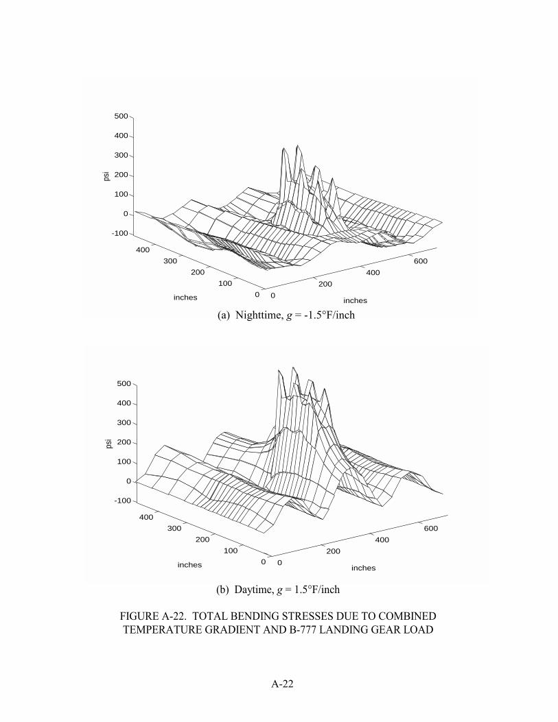
A-22

0

200

400

600

0

100

200

300

400

-100

0

100

200

300

400

500

inchesinches

psi

(a) Nighttime, g = -1.5°F/inch

0

200

400

600

0

100

200

300

400

-100

0

100

200

300

400

500

inchesinches

psi

(b) Daytime, g = 1.5°F/inch

FIGURE A-22. BENDING STRESSES DUE TO COMBINEDTEMPERATURE GRADIENT AND B-777 LANDING GEAR LOAD

TOTAL

0.1

0.06

0.02

-0.02

-0.06

-0.1

0 50 100 150 200 250 300 350 400

L(g = 0) L(g = -1.5) L(g = 1.5) L+T(g = -1.5) L+T(g = 1.5)

Symmetric Axis

(a) Loaded Side

0.1

0.06

0.02

-0.02

-0.06

-0.1

0 50 100 150 200 250 300 350 400

L(g = 0) L(g = -1.5) L(g = 1.5) L+T(g = -1.5) L+T(g = 1.5)

Symmetric Axis

(b) Unloaded Side


FIGURE A-23 . CALCULATED DEFLECTIONS INDUCED BY VARIOUSCOMBINATIONS OF TEMPERATURE GRADIENT AND

B-777 LANDING GEAR LOAD

A-23

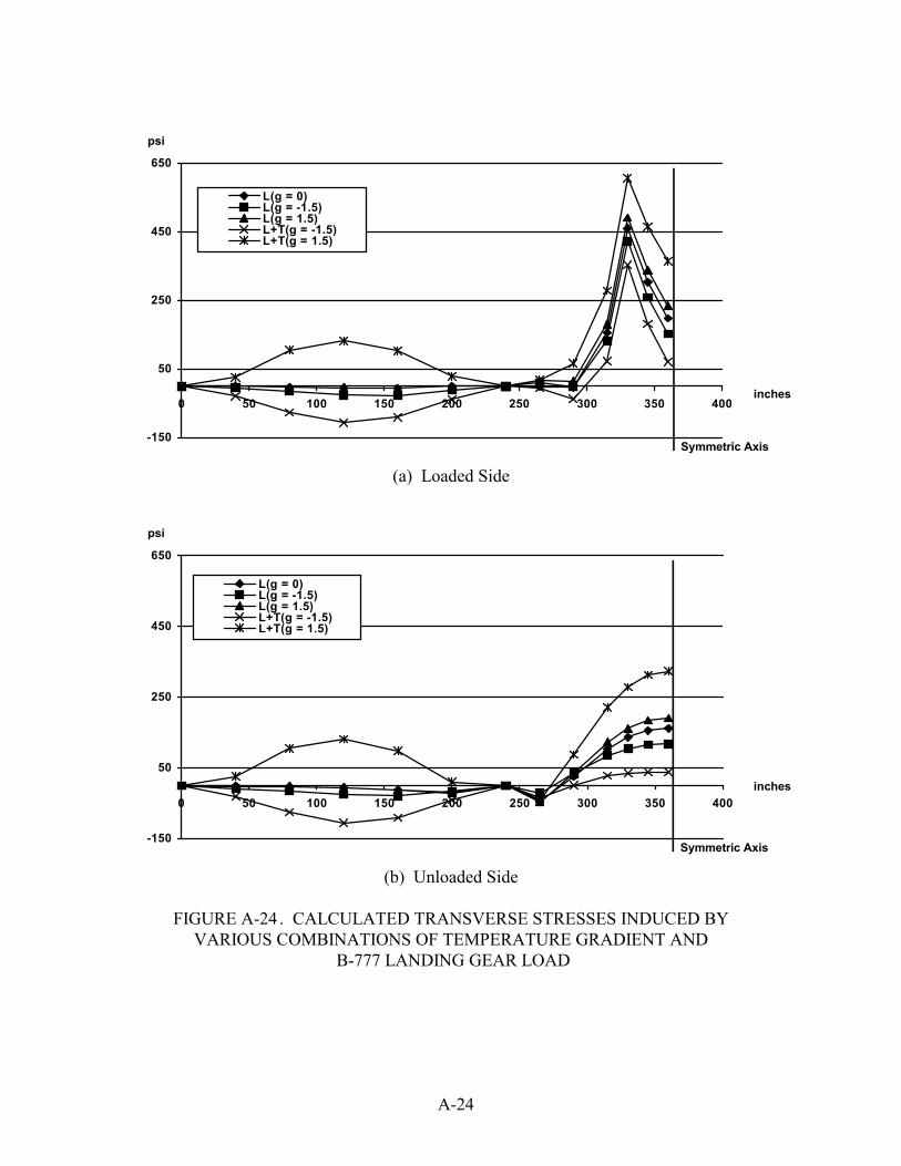
psi

650

450

250

50

inches

-150

0 50 100 150 200 250 300 350 400

L(g = 0) L(g = -1.5) L(g = 1.5) L+T(g = -1.5) L+T(g = 1.5)

Symmetric Axis

(a) Loaded Side

psi

650

450

250

50

inches

-150

0 50 100 150 200 250 300 350 400

L(g = 0) L(g = -1.5) L(g = 1.5) L+T(g = -1.5) L+T(g = 1.5)

Symmetric Axis

(b) Unloaded Side

FIGURE A-24 . CALCULATED TRANSVERSE STRESSES INDUCED BY VARIOUS COMBINATIONS OF TEMPERATURE GRADIENT AND

B-777 LANDING GEAR LOAD

A-24

EFFECT OF SLAB SIZE ON AIRPORT PAVEMENT PERFORMANCE · Effects of Slab Size on Airport Pavement...

Documents

Transcript of EFFECT OF SLAB SIZE ON AIRPORT PAVEMENT PERFORMANCE · Effects of Slab Size on Airport Pavement...