applied sciences

Article

Effect of Coriolis Force on Vibration of Annulus Pipe

Gian Maria Santi * , Daniela Francia and Francesco Cesari

�����������������

Citation: Santi, G.M.; Francia, D.;

Cesari, F. Effect of Coriolis Force on

Vibration of Annulus Pipe. Appl. Sci.

2021, 11, 1058. https://doi.org/

10.3390/app11031058

Academic Editor: Marek Krawczuk

Received: 23 December 2020

Accepted: 21 January 2021

Published: 25 January 2021

Publisher’s Note: MDPI stays neu-

tral with regard to jurisdictional clai-

ms in published maps and institutio-

nal affiliations.

Copyright: © 2021 by the authors. Li-

censee MDPI, Basel, Switzerland.

This article is an open access article

distributed under the terms and con-

ditions of the Creative Commons At-

tribution (CC BY) license (https://

creativecommons.org/licenses/by/

4.0/).

Department of Industrial Engineering—DIN, University of Bologna, Viale del Risorgimento 2,40100 Bologna, Italy; d.francia@unibo.it (D.F.); francesco.cesari@unibo.it (F.C.)* Correspondence: gianmaria.santi2@unibo.it

Abstract: Annulus pipe conveying fluids have many practical applications, such as hydraulic controllines and aircraft fuel lines. In some applications, these tubes are exposed to high speeds. Normally,this leads to a vibration effect which may be of a catastrophic nature. The phenomenon is not onlydriven by the centrifugal forces, but an important role is played also by the Coriolis forces. Manytheoretical approaches exist for a simple configuration or a complex three-dimensional configuration.Finite element models are tested. This paper provides a numerical technique for solving the dynamicsof annulus pipe conveying fluid by means of the mono-dimensional Finite Element Method (FEM).In particular, this paper presents a numerical solution to the equations governing a fluid conveyingpipeline segment, where a Coriolis force effect is taken into consideration both for fix and hingeconstraint.

Keywords: FEM; Coriolis; pipe conveying fluid; simulation

1. Introduction and Background

Fluid conveying pipes [1] are attractive form an engineering point of view becausethe instability effects can be a dangerous structural weakness. These systems interact withaxial flows in flexible conduits with prevalent applications in the oil and gas productionindustries. Examples of these practical applications can be found in [2]. However, theexamples found in the literature are not only limited to the field of engineering but cutacross other areas of human endeavor, such as the study of pulmonary and urinary tractsystems or even hemodynamics within human physiology. A lot of research interest isnow focused on models for studying the stability of certain classes of dynamical systems,finding novel numerical and analytical methods for solving such problems. Thus, for lineardynamics for axial flows along slender structures, the pipe conveying fluid is regarded asthe main paradigm. Direct applications in technical fields can be found in the behavior ofaspirating pipes for ocean mining and Liquefied Natural Gas (LNG) in situ production, aswell as for the offshore mining of methane liquid-crystal deposits and carbon sequestration.Flow-induced vibrations and instabilities are seeking to be resolved by simple, fast, and robustmodels.

Many researchers developed different methodologies to study the problem [3–5]. Inparticular, the Coriolis force became important in the analysis of stability, due to its role inthe energy equation. Studies can be found in [6–8]. Helped by the experiments describedin [9,10] it was possible to assume that the contribution of both the Coriolis force andthe centrifugal force lead to flutter effects that can be dangerous for the strength of thestructure. In [11], Eriksson et al. investigated the impact of the Coriolis force on the longdistance wake behind wind farms by using Large Eddy Simulations (LES) combined witha Forced Boundary Layer (FBL) technique. The results indicate that FBL can be used forstudies of long distance wakes without including a Coriolis correction, but efforts needto be taken to use a wind shear with a correct mean wind veer. The subject of pipingvibration has attracted a lot of attention from various researchers in recent times, due tovast applications. In [12] Shaik et al. described a vibration analysis and mathematical

Appl. Sci. 2021, 11, 1058. https://doi.org/10.3390/app11031058 https://www.mdpi.com/journal/applsci

Appl. Sci. 2021, 11, 1058 2 of 15

model using Euler–Bernoulli and Hamilton’s energy expressions for fluid conveying awelded galvanized iron pipe with a clamped-clamped boundary condition. Many otherattempts concerning the fluid conveying pipe vibrations were made and different analyticalmethods were applied and compared to numerical solutions by software. Avinash B.Kokare et al. [13], studied the vibrational characteristics of pipe conveying fluid andFE simulation to evaluate velocity and pressure distribution in a single phase fluid flow.Gongfa Li et al. [14] obtained the element standard equation for natural frequencies by theLagrangian interpolation function, the first order Hermite interpolation function, and theRitz method. Wentao Xiao et al. [15] used the Lagrangian interpolation function, the firstorder Hermit interpolation function, and the Ritz method to obtain the element standardequation for the nonlinear vibration response and then integrated a global matrix equation,obtaining the response of a conveying fluid pipe with the New Mark method and Matlab.Muhsin J. Jweeg et al. [16] compared results obtained by experimental verification withthe aid of Smart Materials with the results performed by using analytical solution forequation of motion and also, with the results performed by using ANSYS Software. Thefield of nanostructures is currently turning to vibration issues and their formulation aswell. Carbon nanotubes (CNTs) have been extensively used in numerous areas, due totheir excellent mechanical properties. As an important mechanical property, the vibrationcharacteristics of a CNT have become another hot topic for research in recent years. In [17],the spectral element method (SEM) is applied to analyze the dynamic characteristics offluid conveying single-walled carbon nanotubes (SWCNTs).

2. Objectives

This paper proposes a solution to the pipe conveying fluid with Coriolis forces usinga simple one-dimensional Finite Element Method with a Hermitian shape function. Inparticular, the modal frequencies and the critical frequencies are analyzed by changing thevelocity field of the fluid. An imaginary solution is taken into account for the problem,as shown in the following. Mono-dimensional elements make possible the solution ofsimple numerical problems for a complex phenomena, avoiding large Fluid StructureSimulations (FSI) with difficult boundary conditions and numerical issues. In [18], anextensive literature review on the state-of-the-art numerical models in 1D, the Fluid-Structure Interaction is proposed. In the presented paper, two systems are studied: adouble fixed pipe and a hinged pipe to its boundary. The first system is mostly theoretical,while the hinged pipe is more representative of the true environment that can occur ina real application. Engineering solutions are presented for the latter problem, but manyother fields can be researched, such as pulmonary and urinary tract systems in the humanendeavor area, highlighting the importance of simple and fast numerical methods for theanalysis.

3. Methodology

In the modeling of the mechanics of fluid conveying pipes, the Coriolis force wasassigned to have the role of energy absorption that counters the centrifugal effect thatnormally arises in free motions, affecting the stability in conservative and nonconservativesystems, as reported in [1,6–8,19–26]. For example, in [27], sewer condition predictionmodels are developed to provide a framework to forecast future conditions of pipesand to schedule inspection frequencies. Furthermore, in [28], the finite-element methodwas effectively used to model the soil–pipe interaction for five full-scale laboratory testsconducted on a steel pipe. Such models can be used for the analysis of flexible pipeembedment design for layered embedment conditions.

3.1. Analytical Approach

From the studies reported in [29–31], the analytical expression for the motion equationcan be written. Let us start by assuming that the curvature of a pipe in which a fluidflows with a velocity v depends on the transversal displacement w caused by its weight,

Appl. Sci. 2021, 11, 1058 3 of 15

the external forces and the internal forces. Let us assume that m is the total mass of fluidand pipe and ρ is the mass of fluid per length span. If the pipe is immersed in the fluid,it is possible to sum the mass of the external fluid to the mass of the pipe, and it can becalculated by multiplying the density of the fluid itself times the area of the consideredsection. The forces acting on the element dx of the pipe are:

• mw = inertia force due to the vertical acceleration of the pipe;• EJw′′′ = elastic forces due to Euler–Bernoulli’s theory.

E is the Young module of the material, J is the inertia moment of the geometry, andthe derivatives over time and space of the displacement w are defined as follows:

w =dwdt

, w′ =dwdx

, w′′ =d2wdx2 , ω = w′ =

d2wdtdx

When a fluid is flowing in a pipe, and it is subjected to the Coriolis acceleration [32]through the mechanical introduction of the apparent rotation into the pipe, the amountof deflecting force generated by the Coriolis inertial effect will be a function of the massflow rate of the fluid. If a pipe is rotated around a point while a liquid is flowing throughit, that fluid will generate an inertial force acting on the pipe that will be at right angles tothe direction of the flow.

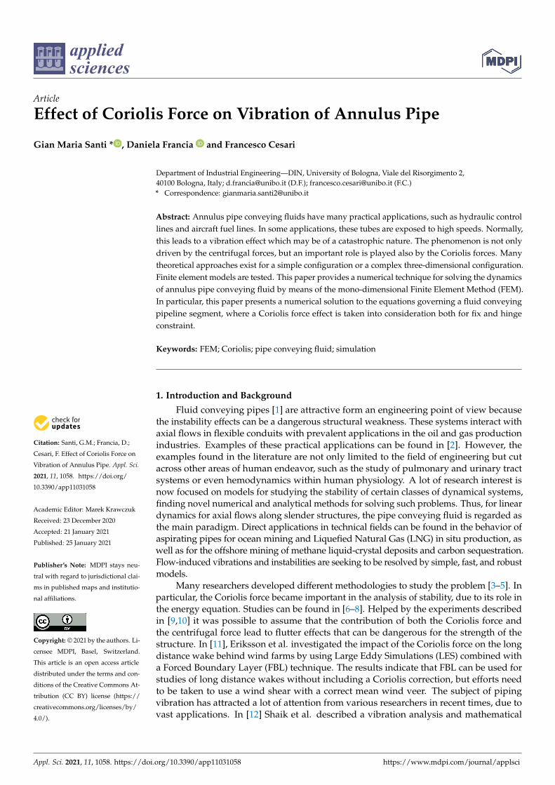
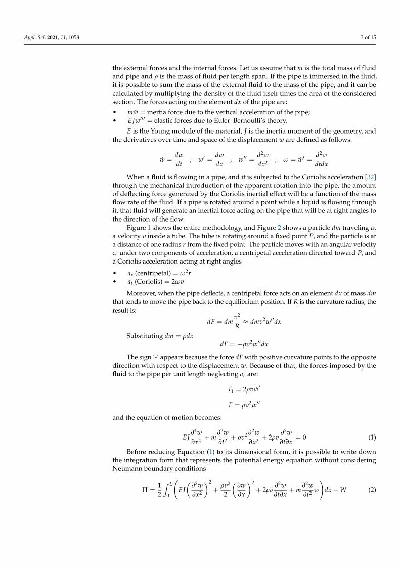
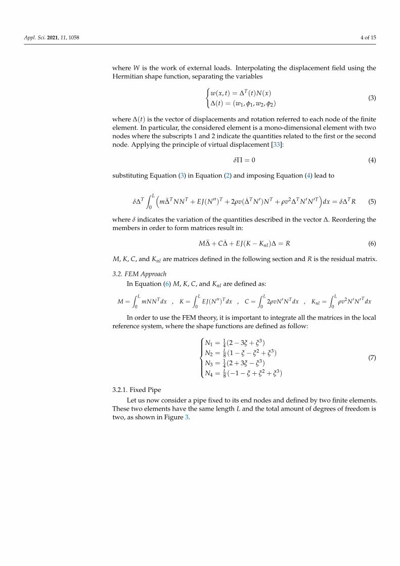
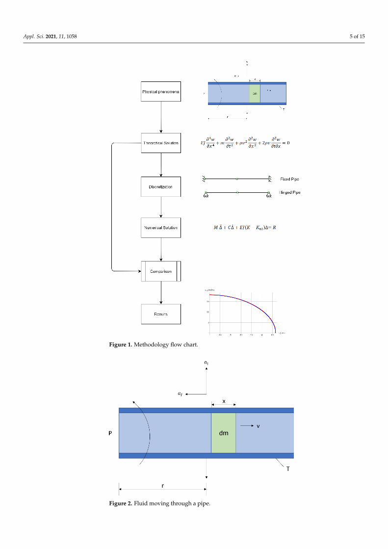
Figure 1 shows the entire methodology, and Figure 2 shows a particle dm traveling ata velocity v inside a tube. The tube is rotating around a fixed point P, and the particle is ata distance of one radius r from the fixed point. The particle moves with an angular velocityω under two components of acceleration, a centripetal acceleration directed toward P, anda Coriolis acceleration acting at right angles

• ar (centripetal) = ω2r• at (Coriolis) = 2ωv

Moreover, when the pipe deflects, a centripetal force acts on an element dx of mass dmthat tends to move the pipe back to the equilibrium position. If R is the curvature radius, theresult is:

dF = dmv2

R≈ dmv2w′′dx

Substituting dm = ρdxdF = −ρv2w′′dx

The sign ‘-’ appears because the force dF with positive curvature points to the oppositedirection with respect to the displacement w. Because of that, the forces imposed by thefluid to the pipe per unit length neglecting ar are:

Ft = 2ρvw′

F = ρv2w′′

and the equation of motion becomes:

EJ∂4w∂x4 + m

∂2w∂t2 + ρv2 ∂2w

∂x2 + 2ρv∂2w∂t∂x

= 0 (1)

Before reducing Equation (1) to its dimensional form, it is possible to write downthe integration form that represents the potential energy equation without consideringNeumann boundary conditions

Π =12

∫ L

0

(EJ(

∂2w∂x2

)2

+ρv2

2

(∂w∂x

)2+ 2ρv

∂2w∂t∂x

+ m∂2w∂t2 w

)dx + W (2)

Appl. Sci. 2021, 11, 1058 4 of 15

where W is the work of external loads. Interpolating the displacement field using theHermitian shape function, separating the variables{

w(x, t) = ∆T(t)N(x)∆(t) = (w1, φ1, w2, φ2)

(3)

where ∆(t) is the vector of displacements and rotation referred to each node of the finiteelement. In particular, the considered element is a mono-dimensional element with twonodes where the subscripts 1 and 2 indicate the quantities related to the first or the secondnode. Applying the principle of virtual displacement [33]:

δΠ = 0 (4)

substituting Equation (3) in Equation (2) and imposing Equation (4) lead to

δ∆T∫ L

0

(m∆T NNT + EJ(N′′)T + 2ρv(∆T N′)NT + ρv2∆T N′N′T

)dx = δ∆T R (5)

where δ indicates the variation of the quantities described in the vector ∆. Reordering themembers in order to form matrices result in:

M∆ + C∆ + EJ(K− Knl)∆ = R (6)

M, K, C, and Knl are matrices defined in the following section and R is the residual matrix.

3.2. FEM ApproachIn Equation (6) M, K, C, and Knl are defined as:

M =∫ L

0mNNTdx , K =

∫ L

0EJ(N′′)Tdx , C =

∫ L

02ρvN′NTdx , Knl =

∫ L

0ρv2N′N′Tdx

In order to use the FEM theory, it is important to integrate all the matrices in the localreference system, where the shape functions are defined as follow:

N1 = 14 (2− 3ξ + ξ3)

N2 = L8 (1− ξ − ξ2 + ξ3)

N3 = 14 (2 + 3ξ − ξ3)

N4 = L8 (−1− ξ + ξ2 + ξ3)

(7)

3.2.1. Fixed Pipe

Let us now consider a pipe fixed to its end nodes and defined by two finite elements.These two elements have the same length L and the total amount of degrees of freedom istwo, as shown in Figure 3.

Appl. Sci. 2021, 11, 1058 5 of 15

Figure 1. Methodology flow chart.

Figure 2. Fluid moving through a pipe.

Appl. Sci. 2021, 11, 1058 6 of 15

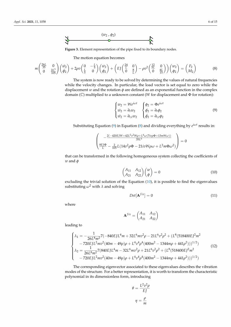
(w2 , φ2)

Figure 3. Element representation of the pipe fixed to its boundary nodes.

The motion equation becomes

m

(26L35 00 2L3

105

)(w2φ2

)+ 2ρv

(0 − L

5L5 0

)(w2φ2

)+

(EJ( 24

L 00 8

L

)− ρv2

( 125L 00 4L

15

))(w2φ2

)=

(F2M2

)(8)

The system is now ready to be solved by determining the values of natural frequencieswhile the velocity changes. In particular, the load vector is set equal to zero while thedisplacement w and the rotation φ are defined as an exponential function in the complexdomain (C) multiplied to a unknown constant (W for displacement and Φ for rotation):

w2 = Weiωt

w2 = ∂tw2

w2 = ∂t,tw2

φ2 = Φeiωt

φ2 = ∂tφ2

φ2 = ∂t,tφ2

(9)

Substituting Equation (9) in Equation (8) and dividing everything by eiωt results in: − 2(−420EJW+42L2v2Wρ+L4ω(7ivρΦ+13mWω))35L3

8EJΦL − 2

105 L(14v2ρΦ− 21ivWρω + L2mΦω2)

= 0

that can be transformed in the following homogeneous system collecting the coefficients ofw and φ (

A11 A12A21 A22

)(wφ

)= 0 (10)

excluding the trivial solution of the Equation (10), it is possible to find the eigenvaluessubstituting ω2 with λ and solving

Det[A f ix] = 0 (11)

where

A f ix =

(A11 A12A21 A22

)leading to

λ1 = − 126L8m2 7(−840EJL4m + 32L6mv2ρ− 21L6v2ρ2 + (L8(518400EJ2m2

− 720EJL2mv2(40m− 49ρ)ρ + L4v4ρ4(400m2 − 1344mρ + 441ρ2)))1/2)

λ2 =1

26L8m2 7(840EJL4m− 32L6mv2ρ + 21L6v2ρ2 + (L8(518400EJ2m2

− 720EJL2mv2(40m− 49ρ)ρ + L4v4ρ4(400m2 − 1344mρ + 441ρ2)))1/2)

(12)

The corresponding eigenvector associated to these eigenvalues describes the vibrationmodes of the structure. For a better representation, it is worth to transform the characteristicpolynomial in its dimensionless form, introducing

θ =L2v2ρ

EJ

η =ρ

m

Appl. Sci. 2021, 11, 1058 7 of 15

so the power of the frequency is

ω2 =EJ

L4m(226.2 + θ(−8.165 + 5.654η)± 0.0385(2.54e7+

106θ(−1.410 + 1.729η) + θ2(19600− 65856η + 21609η2)1/2))

and finally:

Ψ =

√L4mEJ

ω =√∗ (13)

3.2.2. Hinged Pipe

Let us now consider a pipe hinged to its end nodes and defined with two finiteelements. These two elements have the same length L and the total amount of degrees offreedom is 4, as shown in Figure 4.

φ1 (w2 , φ2) φ3

Figure 4. Element representation of the pipe hinged to its boundary nodes.

In this case, the elements of the Equation (6) are defined for four degrees of freedomderived from the imposed boundary condition and result in:

K =ELL3

4L2 −6L 2L2 0−6L 12 −6L 02L2 −6L 4L2 0

0 0 0 0

+ELL3

0 0 0 00 12 6L 6L0 6L 4L2 2L2

0 6L 2L2 4L2

(14a)

M =mL420

4L2 13L −3L2 013L 156 −22L 0−3L2 −22L 4L2 0

0 0 0 0

+mL420

0 0 0 00 156 22L −13L0 22L 4L2 −3L2

0 −13L −3L2 4L2

(14b)

C =2ρv60

0 −6L L2 0

6L 30 −6L 0L2 6L 0 00 0 0 0

+2ρv60

0 0 0 00 −30 −6L 6L0 6L 0 L2

0 −6L −L2 0

(14c)

Knl = ρv2

2L15 − 1

10 − L30 0

− 110

65L − 1

10 0− L

30 − 110

2L15 0

0 0 0 0

+ ρv2

0 0 0 00 6

5L1

101

100 1

102L15 − L

300 1

10 − L30

2L15

(14d)

Following the procedure of the previous case, the unknown quantities are expressedas follows:

w2 = Weiωt

w2 = ∂tw2

w2 = ∂t,tw2

φ1 = Φeiωt

φ1 = ∂tφ1

φ1 = ∂t,tφ1

φ2 = Φeiωt

φ2 = ∂tφ2

φ2 = ∂t,tφ2

φ3 = Φeiωt

φ3 = ∂tφ3

φ3 = ∂t,tφ3

(15)

Substituting Equation (15), Equation (14) in Equation (6), dividing by eiωt and collect-ing the coefficient of ω and φ, it is possible to build the homogeneous system

Appl. Sci. 2021, 11, 1058 8 of 15

A11 A12 A13 A14A21 A22 A23 A24A31 A32 A33 A34A41 A42 A43 A44

wφ1φ2φ3

= 0 (16)

Again, excluding the trivial solution, the natural frequencies are found solving

Det[Ahinge] = 0 (17)

where

Ahinge =

A11 A12 A13 A14A21 A22 A23 A24A31 A32 A33 A34A41 A42 A43 A44

4. Results and Discussions

The results are presented as a comparison between theoretical and numerical solutionsfor simple applications. In particular, a fixed pipe and a hinged pipe are taken into accountas case studies. In both cases, the natural frequencies, due to the geometry only and thevibration modes relative to the inner fluid velocity, are calculated. A steel pipe filled withwater is considered for both applications.

Table 1 shows the data for the following problems. L is the total length, A is the sectionarea, ρ is the fluid density, D is the diameter, d is the thickness, E is the Young module ofthe steel, and m1, m2 are the two masses of the fluid and the pipe.

Table 1. Input data for a steel pipe filled with water.

L = 4 m D = 0.1 m d = 0.095 m

A = πd2

4 m2 E = 2 · 1011 Pa J = π(D2−d2)64

ρ = 1000 πd2

4 m1 = π(D2−d2)4 7800 + 1000A m2 = π(D2−d2)

4 7800

4.1. Fixed Pipe

Considering the pipe only (η = θ = 0 because the mass of the fluid ρ = 0),Equation (13) lets us calculate the two natural frequencies:{

Ψ1 = 5.684Ψ2 = 20.494

against the theoretical values: {Ψ1t = 5.593Ψ2t = 15.417

In particular, the critical loads are calculated solving

Det[EJ( 24

L3 00 8

L

)+ ρv2

(− 12

5L 00 − 4L

15

)] = 0 (18)

thus {θ = 10θ = 30

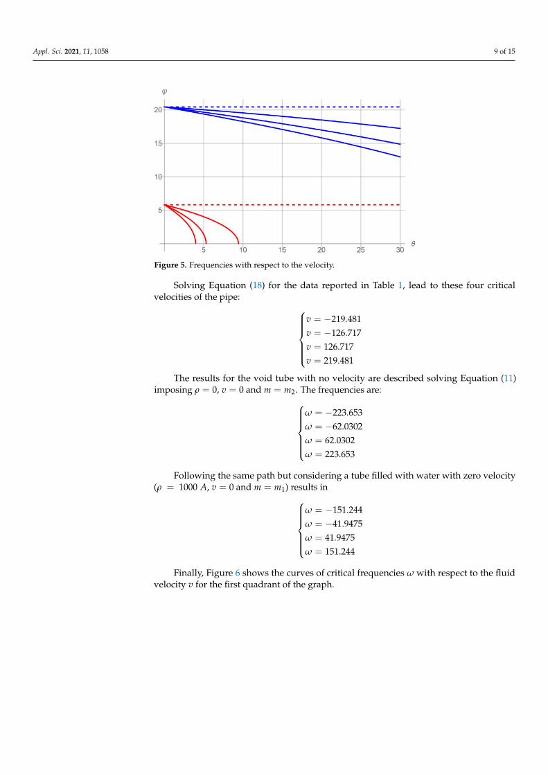
Figure 5 shows the decrease of the frequencies increasing the velocities of the flowunderlying the critical values for the pipe instability (dotted lines).

Appl. Sci. 2021, 11, 1058 9 of 15

Figure 5. Frequencies with respect to the velocity.

Solving Equation (18) for the data reported in Table 1, lead to these four criticalvelocities of the pipe:

v = −219.481v = −126.717v = 126.717v = 219.481

The results for the void tube with no velocity are described solving Equation (11)imposing ρ = 0, v = 0 and m = m2. The frequencies are:

ω = −223.653ω = −62.0302ω = 62.0302ω = 223.653

Following the same path but considering a tube filled with water with zero velocity(ρ = 1000 A, v = 0 and m = m1) results in

ω = −151.244ω = −41.9475ω = 41.9475ω = 151.244

Finally, Figure 6 shows the curves of critical frequencies ω with respect to the fluidvelocity v for the first quadrant of the graph.

Appl. Sci. 2021, 11, 1058 10 of 15

Figure 6. Frequencies respect to the velocity.

4.2. Hinged Pipe

Considering the pipe only and solving Equation (17), it is possible to evaluate thefrequencies:

ω = −2.47714√

EJL4m ω = 2.47714

√EJ

L4m ω = −27.5349√

EJL4m ω = 27.5349

√EJ

L4m

ω = −10.9545√

EJL2√m ω = 10.9545

√EJ

L2√m ω = −50.1996√

EJL2√m ω = 50.1996

√EJ

L2√m

and the theoretical value is:

ωt =π2

4L2

√EJρ

Introducing m = m1 for the fluid mass, it is possible to calculate the frequencies, dueto the water velocity. Figure 7 shows the result for the first frequency.

Figure 7. Frequencies with respect to the velocity.

Figure 8 shows all the four frequencies associated with the finite element solution ofthe hinged structure.

Appl. Sci. 2021, 11, 1058 11 of 15

Figure 8. Frequencies with respect to the velocity.

In this specific application, a comparison with the theoretical solution is possible sinceand the analytical solution is known:

w(x, t) = ∑n

A2n−1 Sin((2n− 1)πxL)Sin(ωit) + ∑

mA2m Sin(2m

πxL)Cos(ωi)t (19)

Equation (19) is substituted in Equation (1). The result can be rewritten by groupingthe trigonometric terms and, in particular, it is possible to expand with a Fourier series thecosines terms:

Cos((−1 + 2n)πx

L

)= ∑

m

2n− 1(2n− 1)2 − (2m)2

Cos(

2mπxL

)= ∑

m

2m(2m)2 − (2n− 1)2

Setting the similar trigonometric terms equal to zero and deleting all the modes exceptfor the first two, the following condition can be written from the homogeneous system

− 32ρvω

3L(

EJπ4

L4 −π2v2ρ

L2 −mω2) = − 3L

8ρvω

(16EJπ4

L4 − 4π2v2ρ

L2 −mω2)

(20)

Equation (20) combined with data in Table 1 defines the critical velocity

vcr = π

√EJρL2

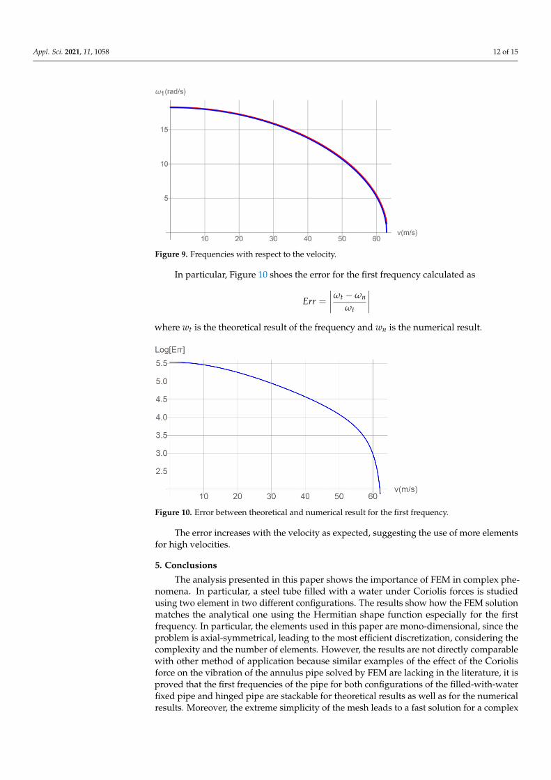
Figure 9 shows the comparison between the theoretical result expressed in Equation (20) andthe numerical result of for the first frequency. The two results match, showing the goodrepresentation offered by a simple discretization of two elements in the finite elementmodel.

Appl. Sci. 2021, 11, 1058 12 of 15

Figure 9. Frequencies with respect to the velocity.

In particular, Figure 10 shoes the error for the first frequency calculated as

Err =∣∣∣∣ωt −ωn

ωt

∣∣∣∣where wt is the theoretical result of the frequency and wn is the numerical result.

Figure 10. Error between theoretical and numerical result for the first frequency.

The error increases with the velocity as expected, suggesting the use of more elementsfor high velocities.

5. Conclusions

The analysis presented in this paper shows the importance of FEM in complex phe-nomena. In particular, a steel tube filled with a water under Coriolis forces is studiedusing two element in two different configurations. The results show how the FEM solutionmatches the analytical one using the Hermitian shape function especially for the firstfrequency. In particular, the elements used in this paper are mono-dimensional, since theproblem is axial-symmetrical, leading to the most efficient discretization, considering thecomplexity and the number of elements. However, the results are not directly comparablewith other method of application because similar examples of the effect of the Coriolisforce on the vibration of the annulus pipe solved by FEM are lacking in the literature, it isproved that the first frequencies of the pipe for both configurations of the filled-with-waterfixed pipe and hinged pipe are stackable for theoretical results as well as for the numericalresults. Moreover, the extreme simplicity of the mesh leads to a fast solution for a complex

Appl. Sci. 2021, 11, 1058 13 of 15

mathematical problem, avoiding heavy three-dimensional meshes and difficult boundaryimpositions.

6. Recommendations for Future Research

A further study should be oriented to the stress distribution, as suggested in [34]in order to investigate mechanical aspects. The use of this method could be very apt toconjure approximate closed form solutions also for nonlinear problems. Further studiesand applications could be aimed also at solving the problem applied to cylindrical shellconveying fluids, whose dynamic behavior is of practical interest in the field of power plantsor oil pipelines. Cylindrical shells are essential structural elements in offshore structures,submarines, and airspace crafts. They are often subjected to combined compressive stressand external pressure, and therefore must be designed to meet strength requirements [35].As discussed in [36], these structures are often stiffened by frames or ribs. Calculation ofthe sound scattering properties of stiffened circular shapes is difficult. Much research hasfocused on the acoustic radiation from a stiffened infinite shell with a simple shape but,when the shape is more complicated, such as for a submarine or an aircraft, the numericalmethods are not appropriate, while the finite element method seems justified with the finiteelement characterizing the stiffeners. This phenomenon could be applied to modern toolssuch as Virtual or Augmented Reality. In particular, Augmented Reality (AR) is a computertechnology where the perception of the user is enhanced by the seamless blending betweena realistic environment and computer-generated virtual objects coexisting in the samespace. The resulting mixture supplements reality, rather than replacing it. The possibilityof interacting with external information could be very useful in simulations difficult to beinterpreted by common users. As suggested in [37–47], Augmented Reality applicationscould have many interesting advantages and could be a viable tool in many fields nowinvestigated by Industry 4.0.

Author Contributions: Conceptualization F.C.; methodology and writing G.M.S.; writing and vali-dation D.F. All authors have read and agreed to the published version of the manuscript.

Funding: This research received no external funding.

Conflicts of Interest: The authors declare no conflict of interest.

Abbreviations

FEM Finite Element MethodLNG Liquefied Natural GasLES Large Eddy SimulationsCTN Carbon NanoTubesSEM Spectral Element MethodSWCNT Single-Walled Carbon NanoTubesFSI Fluid Structure InteractionAR Augmented Reality

References1. Ibrahim, R.A. Overview of Mechanics of Pipes Conveying Fluids—Part I: Fundamental Studies. J. Press. Vessel. Technol. 2010, 132.

[CrossRef]2. Paidoussis, M. Fluid-Structure Interactions: Slender Structures and Axial Flow; Academic Press: Cambridge, MA, USA, 2004;

Volume 2.3. Lee, U. Spectral element modelling and analysis of a pipeline conveying internal unsteady fluid. J. Fluids Struct. 2006, 22, 273–292.

[CrossRef]4. Dodds, H.L.; Runyan, H.L. Effect of High Velocity Fluid Flow on the Bending Vibrations and Static Divergence of a Simply Supported

Pipe; National Aeronautics and Space Administration: Washington, DC, USA, 1965.5. Yamaguchi, R.; Tanaka, G.; Liu, H.; Hayase, T. Fluid Vibration Induced in T-Junction with Double Side Branches. World J. Mech.

2016, 6, 169–179. [CrossRef]6. Kuiper, G.; Metrikine, A. On stability of a clamped-pinned pipe conveying fluid. Heron 2004, 49, 211–232.

Appl. Sci. 2021, 11, 1058 14 of 15

7. Chellapilla, K.R.; Simha, H. Vibrations of Fluid-Conveying Pipes Resting on Two-parameter Foundation. Open Acoust. J. 2008,1, 24–33. [CrossRef]

8. Leklong, J.; Chucheepsakul, S.; Kaewunruen, S. Dynamic Responses of Marine Risers/Pipes Transporting Fluid Subject to Top EndExcitations; Faculty of Engineering, UOW: Wollongong, Australia, 2008.

9. Murai, M.; Yamamoto, M. An Experimental Analysis of the Internal Flow Effects on Marine Risers. Proc. MARTEC 2010, 1,159–165.

10. Marakala, N.; Kuttan, A.K.K.; Kadoli, R. Experimental and Theoretical Investigation of Combined Effect of Fluid and ThermalInduced Vibration on Vertical Thin Slender Tube. Iosr J. Mech. Civ. Eng. 2013, 63–68.

11. Eriksson, O.; Breton, S.P.; Nilsson, K.; Ivanell, S. Impact of Wind Veer and the Coriolis Force for an Idealized Farm to FarmInteraction Case. Appl. Sci. 2019, 9, 922. [CrossRef]

12. Shaik, I.; Uddien, S.; Arkanti, K.; Sutar, S. Numerical Analysis of Clamped Fluid Conveying Pipe. HAL 2017.64.857. [CrossRef]

13. Kokare, A.B.; Paward, P.M. Vibration Characteristics of Pipe Conveying Fluid. Int. J. Sci. Eng. Technol. Res. 2015, 4, 10951–10954.14. Li, G.; Liu, J.; Jiang, G.; Kong, J.; Xie, L.; Xiao, W.; Zhang, Y.; Cheng, F. The nonlinear vibration analysis of the fluid conveying

pipe based on finite element method. Comput. Model. New Technol. 2014, 18, 19–24.15. Li, G.; Xiao, W.; Jiang, G.; Liu, J. Finite element analysis of fluid conveying pipe line of nonlinear vibration response. Comput.

Model. New Technol. 2014, 18, 37–41.16. Jweeg, M.J.; Ntayeesh, T.J. Dynamic analysis of pipes conveying fluid using analytical, numerical and experimental verification

with the aid of smart materials. Int. J. Sci. Res. 2015, 4, 1594–1605.17. Yi, X.; Li, B.; Wang, Z. Vibration Analysis of Fluid Conveying Carbon Nanotubes Based on Nonlocal Timoshenko Beam Theory

by Spectral Element Method. Nanomaterials 2019, 9, 1780. [CrossRef]18. Ferras, D.; Manso, P.; Schleiss, A.; Covas, D. One-Dimensional Fluid-Structure Interaction Models in Pressurized Fluid-Filled

Pipes: A Review. Appl. Sci. 2018, 8, 1844. [CrossRef]19. Elishakoff, I. Controversy Associated with the So-Called “Follower Forces”: Critical Overview. Appl. Mech. Rev. 2005, 58, 117.

[CrossRef]20. Öz, H.R.; Boyaci, H. Transverse vibrations of tensioned pipes conveying fluid with time-dependent velocity. J. Sound Vib. 2000,

236, 259–276. [CrossRef]21. Szmidt, T.; Przybyłowicz, P. Critical flow velocity in a pipe with electromagnetic actuators. J. Theor. Appl. Mech. 2013, 51, 487–496.22. Askarian, A.; Abtahi, H.; Haddadpour, H. Dynamic instability of cantilevered composite pipe conveying flow with an end

nozzle. In Proceedings of the 21st International Congress on Sound and Vibration 2014, ICSV 2014, Beijing, China, 13–17 July2014; Volume 4, pp. 3564–3571.

23. Ntayeesh, T.; Alhelli, A. Free Vibration Characteristics of Elastically Supported Pipe Conveying Fluid. J. Eng. Sci. 2013, 16, 9–19.24. Guo, Q.; Zhang, L.; Xiao, L. Damage analysis of the vehicle’s pipe conveying fluid induced by complex random-shock loads. J.

Press. Equip. Syst. 2006, 4, 100–103.25. Zhang, Y.L.; Gorman, D.G.; Reese, J.M.; Horacek, J. Observations on the vibration of axially tensioned elastomeric pipes conveying

fluid. J. Mech. Eng. Sci. 2000, 214, 423–434. [CrossRef]26. Modarres-Sadeghi, Y.; Païdoussis, M. Nonlinear dynamics of extensible fluid conveying pipes, supported at both ends. J. Fluids

Struct. 2009, 25, 535–543. [CrossRef]27. Sharma, J.; Najafi, M.; Marshall, D.; Kaushal, V.; Hatami, M. Development of a Model for Estimation of Buried Large-Diameter

Thin-Walled Steel Pipe Deflection due to External Loads. J. Pipeline Syst. Eng. Pract. 2019, 10. [CrossRef]28. Malek Mohammadi, M.; Najafi, M.; Kermanshachi, S.; Kaushal, V.; Serajiantehrani, R. Factors Influencing the Condition of Sewer

Pipes: A State-of-the-Art Review. J. Pipeline Syst. Eng. Pract. 2020, 11. [CrossRef]29. Olunloyo, V.O.S.; Osheku, C.A.; Olayiwola, P.S. A Note on an Analytic Solution for an Incompressible Fluid Conveying Pipeline

System. Adv. Acoust. Vib. 2017, 2017, 20. [CrossRef]30. Paidoussis, M.; Issid, N. Dynamic stability of pipes conveying fluid. J. Sound Vib. 1974, 33, 267–294. [CrossRef]31. Semler, C.; Li, G.; Paidoussis, M. The Non-linear Equations of Motion of Pipes Conveying Fluid. J. Sound Vib. 1994, 169, 577–599.

[CrossRef]32. Enz, S.; Thomsen, J.J. Predicting phase shift effects for vibrating fluid conveying pipes due to Coriolis forces and fluid pulsation.

J. Sound Vib. 2011, 330, 5096–5113. [CrossRef]33. Bathe, K. Finite Element Procedures in Engineering Analysis; Prentice Hall Inc.: Upper Saddle River, NJ, USA, 2014.34. Zachwieja, J. Stress analysis of vibrating pipelines. Aip Conf. Proc. 2017, 1822, 020017. [CrossRef]35. Bai, Y.; Jin, W.L. Ultimate Strength of Cylindrical Shells; Elsevier: Oxford, UK, 2016; pp. 353–365. [CrossRef]36. Debus, J.C. 4-Finite element analysis of flexural vibration of orthogonally stiffened cylindrical shells with ATILA. In Applications

of ATILA FEM Software to Smart Materials; Uchino, K., Debus, J.C., Eds.; Woodhead Publishing Series in Electronic and OpticalMaterials; Woodhead Publishing: New Delhi, India, 2013; pp. 69–93. [CrossRef]

37. Ceruti, A.; Marzocca, P.; Liverani, A.; Bil, C. Maintenance in aeronautics in an Industry 4.0 context: The role of AugmentedReality and Additive Manufacturing. J. Comput. Des. Eng. 2019, 6, 516–526. [CrossRef]

Appl. Sci. 2021, 11, 1058 15 of 15

38. Osti, F.; Ceruti, A.; Liverani, A.; Caligiana, G. Semi-automatic Design for Disassembly Strategy Planning: An Augmented RealityApproach. In Proceedings of the 27th International Conference on Flexible Automation and Intelligent Manufacturing, FAIM2017,Modena, Italy, 27–30 June 2017; Volume 11, pp. 1481–1488. [CrossRef]

39. Frizziero, L.; Liverani, A.; Caligiana, G.; Donnici, G.; Chinaglia, L. Design for disassembly (DfD) and augmented reality (AR):Case study applied to a gearbox. Machines 2019, 7, 29. [CrossRef]

40. De Marchi, L.; Ceruti, A.; Marzani, A.; Liverani, A. Augmented Reality to Support On-Field Post-Impact Maintenance Operationson Thin Structures. J. Sens. 2013, 2013, 619570. [CrossRef]

41. Liverani, A.; Leali, F.; Pellicciari, M. Real-time 3D features reconstruction through monocular vision. Int. J. Interact. Des. Manuf.2010, 4, 103–112. [CrossRef]

42. Liverani, A.; Kuester, F.; Hamann, B. Towards interactive finite element analysis of shell structures in virtual reality. InProceedings of the 1999 IEEE International Conference on Information Visualization (Cat. No. PR00210), London, UK, 14–16 July1999; pp. 340–346. [CrossRef]

43. Francia, D.; Seminerio, D.; Caligiana, G.; Frizziero, L.; Liverani, A.; Donnici, G. Virtual Design for Assembly Improving theProduct Design of a Two-Way Relief Valve. In Proceedings of the International Conference on Design, Simulation, Manufacturing:The Innovation Exchange, Kharkiv, Ukraine, 9–12 June 2020; pp. 304–314. [CrossRef]

44. Osti, F.; Santi, G.C.G. Real Time Shadow Mapping for Augmented Reality Photorealistic Rendering. Appl. Sci. 2019, 9, 2225.[CrossRef]

45. Francia, D.; Ponti, S.; Frizziero, L.; Liverani, A. Virtual Mechanical Product Disassembly Sequences Based on Disassembly OrderGraphs and Time Measurement Units. Appl. Sci. 2019, 9, 3638. [CrossRef]

46. Amicis, R.; Ceruti, A.; Francia, D.; Frizziero, L.; Simões, B. Augmented Reality for virtual user manual. Int. J. Interact. Des. Manuf.2018, 12. [CrossRef]

47. Frizziero, L.; Donnici, G.; Caligiana, G.; Liverani, A.; Francia, D. Project of Inventive Ideas Through a TRIZ Study Applied to theAnalysis of an Innovative Urban Transport Means. Int. J. Manuf. Mater. Mech. Eng. 2018, 8, 35–62. [CrossRef]