EE4-65/EE9-SO27 Wireless Communications · EE4-65/EE9-SO27 Wireless Communications Bruno Clerckx...
273
EE4-65/EE9-SO27 Wireless Communications Bruno Clerckx Department of Electrical and Electronic Engineeing, Imperial College London January 2016 1 / 273
Transcript of EE4-65/EE9-SO27 Wireless Communications · EE4-65/EE9-SO27 Wireless Communications Bruno Clerckx...

EE4-65/EE9-SO27 Wireless Communications
Bruno Clerckx
Department of Electrical and Electronic Engineeing, Imperial College London
January 2016
1 / 273

Course Ojectives
• Advanced course on wireless communication and communication theory– Provides the fundamentals of wireless communications from a 4G and beyond
perspective– At the cross-road between information theory, coding theory, signal processing and
antenna/propagation theory
• Major focus of the course is on MIMO (Multiple Input Multiple Output) andmulti-user/multi-cell communications
– Includes as special cases SISO (Single Input Single Output), MISO (Multiple InputSingle Output), SIMO (Single Input Multiple Output)
– Applications: everywhere in wireless communication networks: 3G, 4G(LTE,LTE-A),(5G?), WiMAX(IEEE 802.16e, IEEE 802.16m), WiFi(IEEE 802.11n), satellite,...+ inother fields, e.g. radar, medical devices, speech and sound processing, ...
• Valuable for those who want to either pursue a PhD in communication or a career ina high-tech telecom company (research centres, R&D branches of telecommanufacturers and operators,...).
• Skills– Mathematical modelling and analysis of (MIMO-based) wireless communication
systems– Design (transmitters and receivers) of multi-cell multi-user MIMO wireless
communication systems– Practical understanding of MIMO applications and performance evaluations
2 / 273

Content
Central question: How to deal with fading and interference in wireless networks?
• Some fundamentals/revision (matrix analysis, probability, information theory)• Single link: point to point communications
– Fading and Diversity– MIMO Channels - Modelling and Propagation– Capacity of point-to-point MIMO Channels– Space-Time Coding/Decoding over I.I.D. Rayleigh Flat Fading Channels– Partial Channel State Information at the Transmitter (CSIT)
• Multiple links: multiuser communications– Multi-User MIMO - Capacity of Multiple Access Channels (Uplink)– Multi-User MIMO - Capacity of Broadcast Channels (Downlink)– Multi-User MIMO - Scheduling, Linear Precoding (Downlink)
• Multiple cells: multiuser multicell communications– Introduction to Multi-Cell MIMO– Capacity of Interference Channel
• Real-World MIMO Wireless Networks– MIMO and Interference Management in 4G and beyond (LTE, LTE-Advanced,
WiMAX)
3 / 273

Important Information
• Course webpage: http://www.ee.ic.ac.uk/bruno.clerckx/Teaching.html
• Prerequisite: EE9SC2 Advanced Communication Theory
• Lectures on Tuesday from 14.00 till 16.00
• Exam (written, 3 hours, closed book): 70%; Project (using Matlab): 30%.
• Do the problems in problem sheets (2 types: 1. paper/pencil, 2. matlab)
• Project– to be distributed around mid February (details to come later)– report to be submitted by end of March (details to come later).
4 / 273

Important Information
• Reference book
Bruno Clerckx and Claude Oestges,“MIMO Wireless Networks: Channels,Techniques and Standards for Multi-Antenna, Multi-User and Multi-CellSystems,” Academic Press (Elsevier),Oxford, UK, Jan 2013.
• Another interesting reference on wireless communications (more introductory)“Fundamentals of Wireless Communication,” by D. Tse and P. Viswanath,Cambridge University Press, May 2005
5 / 273

Some fundamentals/revisions (matrix analysis,probability)
6 / 273

Reference Book
• Bruno Clerckx and Claude Oestges, “MIMO Wireless Networks: Channels,Techniques and Standards for Multi-Antenna, Multi-User and Multi-Cell Systems,”Academic Press (Elsevier), Oxford, UK, Jan 2013.
– Appendix A, B
7 / 273

Matrix properties
• Vector Orthogonality : aHb = 0 (H stands for Hermitian, i.e. conjugate transpose)• Hermitian matrix : A = AH
• Unitary matrix : AHA = I
• Singular Value Decomposition (SVD) of a matrix H [nr × nt]: H = UΣVH
– U [nr × r(H)]: unitary matrix of left singular vectors– Σ = diagσ1, σ2, . . . , σr(H): diagonal matrix containing the singular values of H
– V [nt × r(H)]: unitary matrix of left singular vectors– r(H): the rank of H
We will often look at Hermitian matrices of the form A = HHH whose EigenvalueValue Decomposition (EVD) writes as A = VΛVH with Λ = Σ2.
• A = HHH is a positive-semidefinite matrix (≥ 0), i.e. all eigenvalues of A arenonnegative.
• Trace of a matrix A: Tr A =∑i A(i, i).• Frobenius norm of a matrix A: ‖A‖2F =
∑
i
∑
j |A(i, j)|2
• ‖A‖2F = TrAAH
= Tr
AHA
• Tr AB = Tr BA• det (I+AB) = det (I+BA)• Hadamard’s inequality : det (A) ≤∏n
k=1 A (k, k) if A > 0 (positive definite matrix,all eigenvalues are positive) of size n× n
8 / 273

Matrix properties
• Kronecker product:A⊗B =
A(1, 1)B . . . A(1, n)B... . . .
...,A(m, 1)B . . . A(m,n)B
• (A⊗B)⊗C = A⊗ (B⊗C)• (A⊗B)H = AH ⊗BH
• (A⊗B) (C⊗D) = (AC⊗BD)• (A⊗B)−1 = A−1 ⊗B−1 if A,B square and non singular.• det (Am×m ⊗Bn×n) = det (A)n det (B)m
• Tr A⊗B = Tr ATr B• Tr AB ≥ Tr Aσ2
min (B) with σmin (B) the smallest singular value of B• vec (A) converts [m× n] matrix into mn× 1 vector by stacking the columns of A
on top of one another.– vec (ABC) =
(CT ⊗A
)vec (B)
• TrABBHAH
= vec
(AH
)H (I⊗BBH
)vec(AH
)
• det (I+ ǫA) = 1 + ǫTr A if ǫ << 1
9 / 273

Gaussian random variable
• Real Gaussian random variable x with mean µ = E x and variance σ2
p (x) =1√2πσ2
exp
(
− (x− µ)2
2σ2
)
.
Standard Gaussian random variable: µ = 0 and σ2 = 1• Real Gaussian random vector x of dimension n with mean vector µ = E x and
covariance matrix R = E
(x− µ) (x− µ)T
:
p (x) =1
(√2π)n√
det (R)exp
(
− (x− µ)T R−1 (x− µ)
2
)
.
Standard Gaussian random vector x of dimension n: entries are independent andidentically distributed (i.i.d.) standard Gaussian random variables x1, . . . , xn
p (x) =1
(√2π)n exp
(
−‖x‖2
2
)
.
10 / 273

Gaussian random variable
• Complex Gaussian random variable x = xr + jxi: [xr, xi]T is a real Gaussian
random vector.• Important case: x = xr + jxi is such that its real and imaginary parts are i.i.d. zero
mean Gaussian variables of variance σ2 (circularly symmetric complex Gaussianrandom variable).
• s = |x| =√
x2r + x2
i is Rayleigh distributed
p(s) =s
σ2exp
(
− s2
2σ2
)
.
• y = s2 = |x|2 = x2r + x2
i is χ22 (i.e. exponentially) distributed (with two degrees of
freedom)
py(y) =1
2σ2exp
(
− y
2σ2
)
.
Hence, µ = E y = 2σ2.• More generally, χ2
n is the sum of the square of n i.i.d. zero-mean Gaussian randomvariables.
• Assume n i.i.d. zero mean complex Gaussian variables h1, . . . , hn (real and imaginaryparts with variance σ2). Defining u =
∑nk=1 |hk|2, the MGF of u is given by
Mu(τ ) = Eeτu =[
1
1− 2σ2τ
]n
,
11 / 273

Appendix: Basics of Information Theory
T. Cover and J. Thomas, “Elements of Information Theory,” SecondEdition, Wiley, 2006.
12 / 273

Discrete Memoryless Channel
Definition
A discrete channel is defined as a system consisting of an input alphabet X andoutput alphabet Y and a probability transition matrix p(y|x) that expresses theprobability of observing the output symbols y given that the symbold x is sent.
Definition
The channel is memoryless if the probability distribution of the output dependsonly on the input at that time and is conditionally independent of previouschannel inputs or outputs, i.e. if x1,...,xn are inputs, and y1,...,yn denote thecorresponding outputs, for n channel uses, then
p(y1, ..., yn|x1, ...xn) = p(y1|x1)...p(yn|xn)
Example
Binary Symmetric Channel (BSC): x and y take values in 0,1 such that
p(y|x) =
1− p, y = x,p, y = 1− x.
13 / 273

Entropy
• Entropy is a measure of the average uncertainty of a random variable
Definition
For a discrete random variable X, the entropy H(X) is defined as
H(X) = E
log21
p(X)
= −E log2 p(X) = −∑
x
p(x) log2 p(x),
where p(x) is the probability mass function of X.
• It is the number of bits on average required to describe the random variable.
Example
Let X be a Bernoulli random variable
X =
1, with probability p,0, with probability 1− p.
Then H(X) = −p log2 p− (1− p) log2(1− p). For p = 0, 1, there is nouncertainty on the value of the RV, so no information gained. For p = 1/2,H(X) (uncertainty/information) is maximized.
14 / 273

Entropy
Lemma
H(X) ≥ 0
Proof: 0 ≤ p(x) ≤ 1 such that log21
p(x)≥ 0
Definition
The joint entropy H(X,Y ) of a pair of discrete random variables X and Ywith a joint pmf p(x, y) is defined as
H(X,Y ) = −E log2 p(X,Y ) = −∑
x
∑
y
p(x, y) log2 p(x, y)
15 / 273

Conditional Entropy
• The conditional entropy of a random variable given another is the expected value ofthe entropies of the conditional distributions, averaged over the conditioning randomvariable
Definition
The conditional entropy H(Y |X) is defined as
H(Y |X) =∑
x
p(x)H(Y |X = x)
= −∑
x
p(x)∑
y
p(y|x) log2 p(y|x)
= −∑
x
∑
y
p(x, y) log2 p(y|x)
= −E log2 p(Y |X)
16 / 273

Joint Entropy
Theorem
Chain ruleH(X,Y ) = H(X) +H(Y |X)
Proof:
H(X,Y ) = −∑
x
∑
y
p(x, y) log2 p(x, y) = −∑
x
∑
y
p(x, y) log2 p(x)p(y|x)
= −∑
x
∑
y
p(x, y) log2 p(x)−∑
x
∑
y
p(x, y) log2 p(y|x)
= −∑
x
p(x) log2 p(x)−∑
x
∑
y
p(x, y) log2 p(y|x)
= H(X) +H(Y |X)
Alternatively,
log2 p(X,Y ) = log2 p(X) + log2 p(Y |X)
E log2 p(X,Y ) = E log2 p(X)+ E log2 p(Y |X)17 / 273

Relative Entropy
• The relative entropy is a measure of the distance between two distributions.
Definition
The relative entropy between two pmf p(x) and q(x) is defined as
D(p||q) =∑
x
p(x) log2p(x)
q(x)= Ep
log2p(X)
q(X)
Theorem
The relative entropy is always nonnegative D(p||q) ≥ 0 and is zero if and onlyif p = q.
18 / 273

Mutual Information
• The mutual information is a measure of the amount of information that one RVcontains about another RV. It is a measure of the dependence between the two RVs.
Definition
For a pair of discrete random variables X and Y with a joint pmf p(x, y) andmarginal pmf p(x) and p(y), the mutual information I(X;Y ) is the relativeentropy between p(x, y) and p(x)p(y)
I(X;Y ) = D(p(x, y)||p(x)p(y)) = Ep(x,y)
log2p(X,Y )
p(X)p(Y )
=∑
x
∑
y
p(x, y) log2
p(x, y)
p(x)p(y)
19 / 273

Mutual Information
• The mutual information I(X;Y ) is the reduction in the uncertainty of one randomvariable due to the knowledge of the other
I(X;Y ) =∑
x,y
p(x, y) log2
p(x, y)
p(x)p(y)
=∑
x,y
p(x, y) log2
p(x|y)p(x)
= −∑
x,y
p(x, y) log2 p(x) +∑
x,y
p(x, y) log2 p(x|y)
= −∑
x
p(x) log2 p(x)−(
−∑
x,y
p(x, y) log2 p(x|y))
= H(X)−H(X|Y )
= H(Y )−H(Y |X) = I(Y ;X)
• I(X;Y ) = H(X) +H(Y )−H(X,Y ).• I(X;X) = H(X)−H(X|X) = H(X)
20 / 273

Mutual Information
Theorem
Nonnegativity of mutual information: For any two random variables X,Y
I(X;Y ) ≥ 0
with equality if and only if X and Y are independent
Theorem
Conditioning reduces entropy: For any two random variables X,Y
H(X|Y ) ≤ H(X)
with equality if and only if X and Y are independent
Proof: 0 ≤ I(X;Y ) = H(X)−H(X|Y )
Knowing another RV Y can only reduce on the average the uncertainty in X.
21 / 273

Channel Coding Theorem
Theorem
(a) For a DMC with channel transition pmf p(y|x), we can use i.i.d. inputswith pmf p(x) to communicate reliably, as long as the code rate satisfies
R < I(X;Y ).
(b) The achievable rate can be maximized over the input density p(x) to obtainthe channel capacity
C = maxp(x)
I(X;Y ).
22 / 273

Differential Entropy
Definition
For a continuous random variable X, the differential entropy h(X) is defined as
h(X) = E
log21
p(x)
= −E log2 p(x) = −∫
p(x) log2 p(x)dx,
where p(x) is the probability density function of X.
Caution: h(X) can be negative.
Example
For X ∼ N(µ, σ2), − log2 p(x) =(x−µ)2
2σ2 log2(e) +12log2(2πσ
2). Thus,
h(X) = −E log2 p(x) = 12log2(e) +
12log2(2πσ
2) = 12log2(2πeσ
2). Themean does not affect the differential entropy.
Theorem
Consider a RV with zero mean and variance σ2. Then h(X) ≤ 12log2(2πeσ
2),with equality iff X ∼ N(0, σ2).
23 / 273

AWGN Channel
• Real discrete-time AWGN channel
Y = X +N, N ∼ N(0, σ2)
where X is power-constrained input EX2≤ Es
• The channel transition density is given by
p(y|x) = 1√2πσ2
exp
(
− (y − x)2
2σ2
)
24 / 273

AWGN Channel Capacity
Theorem
The capacity of the real AWGN channel is
C = maxp(x):EX2≤Es
I(X;Y ) =1
2log2(1 +
Es
σ2).
Proof: Consider Y = X +N , with N ∼ N(0, σ2) and EX2≤ Es. Given X = x,
h(Y |X = x) = h(N), so that h(Y |X) = h(N) and
I(X;Y ) = h(Y )− h(Y |X) = h(Y )− h(N).
Maximizing I(X;Y ) comes to maximize h(Y ). Since X and N are independent,EY 2= E
X2+ E
N2≤ Es + σ2. We now know that
h(Y ) ≤ 1
2log2(2πe(Es + σ2))
and equality is achieved iff Y ∼ N(0, Es + σ2). Y ∼ N(0, Es + σ2) is achieved ifthe input distribution is X ∼ N(0, Es), independent of the noise. We then get
I(X;Y ) = h(Y )−h(N) =1
2log2(2πe(Es+σ2))− 1
2log2(2πeσ
2) =1
2log2(1+
Es
σ2).
25 / 273

Jensen’s inequality
Theorem
If f is a convex function and X is a random variable,
E f(X) ≥ f(E X).
26 / 273

Fading and Diversity
27 / 273

Reference Book
• Bruno Clerckx and Claude Oestges, “MIMO Wireless Networks: Channels,Techniques and Standards for Multi-Antenna, Multi-User and Multi-Cell Systems,”Academic Press (Elsevier), Oxford, UK, Jan 2013.
– Chapter 1
Section: 1.2, 1.3, 1.4, 1.5Appendix A, B
28 / 273

Space-Time Wireless Channels:Discrete TimeRepresentation
• channel : the impulse response of the linear time-varying communication systembetween one (or more) transmitter(s) and one (or more) receiver(s).
• Assume a SISO transmission where the digital signal is defined in discrete-time bythe complex time series cll∈Z and is transmitted at the symbol rate Ts.
• The transmitted signal is then represented by
c(t) =∞∑
l=−∞
√Esclδ(t− lTs),
where Es is the transmitted symbol energy, assuming that the average energyconstellation is normalized to unity.
• Define a function hB(t, τ ) as the time-varying (along variable t) impulse response ofthe channel (along τ ) over the system bandwidth B = 1/Ts, i.e. hB(t, τ ) is theresponse at time t to an impulse at time t− τ .
• The received signal y(t) is given by
y(t) = hB(t, τ ) ⋆ c(t) + n(t)
=
∫ τmax
0
hB(t, τ )c(t− τ )dτ + n(t)
where ⋆ denotes the convolution product, n(t) is the additive noise of the system andτmax is the maximal length of the impulse response.
29 / 273

Discrete Time Representation
• hB is a scalar quantity, which can be further decomposed into three main terms,
hB(t, τ ) = fr ⋆ h(t, τ ) ⋆ ft,
where– ft is the pulse-shaping filter,– h(t, τ) is the electromagnetic propagation channel (including the transmit and receive
antennas) at time t,– fr is the receive filter.
• Nyquist criterion: the cascade f = fr ⋆ ft does not create inter-symbol interferencewhen y(t) is sampled at rate Ts.
• In practice,– difficult to model h(t, τ) (infinite bandwidth is required).– hB(t, τ) is usually the modeled quantity, but is written as h(t, τ) (abuse of notation).– Same notational approximation: the channel impulse response writes as h(t, τ) or ht[τ ].
• The input-output relationship reads thereby as
y(t) = h(t, τ ) ⋆ c(t) + n(t) =∞∑
l=−∞
√Esclht[t− lTs] + n(t).
30 / 273

Discrete Time Representation
• Sampling the received signal at the symbol rate Ts (yk = y(t0 + kTs), using theepoch t0) yields
yk =∞∑
l=−∞
√Esclht0+kTs [t0 + (k − l)Ts] + n(t0 + kTs)
=
∞∑
l=−∞
√Esclhk[k − l] + nk
Example
At time k = 0, the channel has two taps: h0[0], h0[1]
y0 =√Es [c0h0[0] + c−1h0[1]] + n0
• If Ts >> τmax,– hB(t, τ) is modeled by a single dependence on t: write simply as hB(t) (or h(t) using
the same abuse of notation). In the sampled domain, hk = h(t0 + kTs).– the channel is then said to be flat fading or narrowband
yk =√
Eshkck + nk
• Otherwise the channel is said to be frequency selective.31 / 273

Path-Loss and Shadowing
• Assuming narrowband channels and given specific Tx and Rx locations, hk ismodeled as
hk =1√Λ0 S
hk,
where– path-loss Λ0: a real-valued deterministic attenuation term modeled as Λ0 ∝ Rη whereη designates the path-loss exponent and R the distance between Tx and Rx.
– shadowing S: a real-valued random additional attenuation term, which, for a givenrange, depends on the specific location of the transmitter and the receiver and modeledas a lognormal variable, i.e., 10 log10(S) is a zero-mean normal variable of givenstandard deviation σS .
– fading hk: caused by the combination of non coherent multipaths. By definition of Λ0
and S, E|h|2
= 1.
• Alternatively, hk = Λ−1/2 hk with Λ modeled on a logarithm scale
Λ|dB = Λ0|dB + S|dB = L0|dB + 10η log10
(R
R0
)
+ S|dB,
where |dB indicates the conversion to dB, and L0 is the deterministic path-loss at areference distance R0, and Λ is generally known as the path-loss.
32 / 273

Path-Loss and Shadowing
• Path loss models are identical for both single- and multi-antenna systems.
• For point to point systems, it is common to discard the path loss and shadowing andonly investigate the effect due to fading, i.e. the classical model for narrowbandchannels
y =√Eshc+ n,
where the time index is removed for better legibility and n is usually taken as whiteGaussian distributed, E
nkn
∗l
= σ2
nδ(k − l).
• Es can then be seen as an average received symbol energy. The average SNR is thendefined as ρ , Es/σ
2n.
33 / 273
Fading
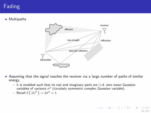
• Multipaths
transmitter
line-of-sight
diffusion
receiver
diffraction
specular reflection
• Assuming that the signal reaches the receiver via a large number of paths of similarenergy,
– h is modeled such that its real and imaginary parts are i.i.d. zero mean Gaussianvariables of variance σ2 (circularly symmetric complex Gaussian variable).
– Recall E|h|2
= 2σ2 = 1.
34 / 273

Fading
• The channel amplitude s , |h| follows a Rayleigh distribution,
ps(s) =s
σ2exp
(
− s2
2σ2
)
,
whose first two moments are
Es = σ
√π
2
Es2 = 2σ2 = E|h|2
= 1.
• The phase of h is uniformly distributed over [0, 2π)
35 / 273
Fading
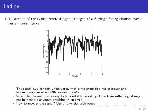
• Illustration of the typical received signal strength of a Rayleigh fading channel over acertain time interval
0 1 2 3 4 5−30
−25
−20
−15
−10
−5
0
5
10
Time [s]
Rec
eive
d si
gnal
[dB
]
– The signal level randomly fluctuates, with some sharp declines of power andinstantaneous received SNR known as fades.
– When the channel is in a deep fade, a reliable decoding of the transmitted signal maynot be possible anymore, resulting in an error.
– How to recover the signal? Use of diversity techniques
36 / 273

Maximum likelihood detection
• Decision rule: choose the hypothesis that maximizes the conditional density
argmaxx
p(y|x) = argmaxx
log p(y|x)
• If real AWGN y = x+ n with n ∼ N(0, σ2n),
p(y|x) = 1√2πσ2
n
exp
(
− (y − x)2
2σ2n
)
andargmax
xp(y|x) = argmin
x(y − x)2
• If y =√Eshc+ n, the ML decision rule becomes
argminc
∣∣∣y −
√Eshc
∣∣∣
2
37 / 273

Diversity in Multiple Antennas Wireless Systems
• What is the impact of fading on system performance?• Consider the simple case of BPSK transmission through an AWGN channel and a
SISO Rayleigh fading channel:– In the absence of fading (h = 1), the symbol-error rate (SER) in an additive white
Gaussian noise (AWGN) channel is given by
P = Q(√
2Es
σ2n
)
= Q(√
2ρ),
where Q (x) is the Gaussian Q-function defined as
Q (x)∆= P (y ≥ x) = 1√
2π
∫ ∞
xexp
(
−y2
2
)
dy.
– In the presence of (Rayleigh) fading, the received signal level fluctuates as s√Es, and
the SNR varies as ρs2. As a result, the SER
P =
∫ ∞
0Q(√
2ρs)ps(s) ds
=1
2
(
1−√
ρ
1 + ρ
)
(ρր)∼= 1
4ρ
although the average SNR ρ =∫∞0 ρs2 ps(s) ds remains equal to ρ.
38 / 273

Diversity in Multiple Antennas Wireless Systems
• How to combat the impact of fading? Use diversity techniques• The principle of diversity is to provide the receiver with multiple versions (called
diversity branch) of the same transmitted signal.– Independent fading conditions across branches needed.– Diversity stabilizes the link through channel hardening which leads to better error rate.– Multiple domains: time (coding and interleaving), frequency (equalization and
multi-carrier modulations) and space (multiple antennas/polarizations).
• Array Gain: increase in average output SNR (i.e., at the input of the detector)relative to the single-branch average SNR ρ
ga ,ρoutρ
=ρoutρ
• Diversity Gain: increase in the error rate slope as a function of the SNR. Defined asthe negative slope of the log-log plot of the average error probability P versus SNR
god(ρ) , −log2
(P)
log2 (ρ).
The diversity gain is commonly taken as the asymptotic slope, i.e., for ρ→∞.
39 / 273

Diversity in Multiple Antennas Wireless Systems
• Illustration of diversity and array gains
SNR ρ [dB]
Err
or
pro
ba
bili
ty
diversity gain
= slope increase
AWGNRayleigh fading, no spatial diversityRayleigh fading with diversity
array gain = SNR shift Careful that the curves have beenplotted against the single-branchaverage SNR ρ = ρ !If plotted against the output aver-age SNR ρout, the array gain dis-appears.
• Coding Gain: a shift of the error curve (error rate vs. SNR) to the left, similarly tothe array gain.
– If the error rate vs. the average receive SNR ρout, any variation of the array gain isinvisible but any variation of the coding gain is visible: for a given SNR level ρout atthe input of the detector, the error rates will differ.
40 / 273

SIMO Systems
• Receive diversity may be implemented via two rather different combining methods:– selection combining : the combiner selects the branch with the highest SNR among thenr receive signals, which is then used for detection,
– gain combining : the signal used for detection is a linear combination of all branches,z = gy, where g = [g1, . . . , gnr ] is the combining vector.
1 Equal Gain Combining2 Maximal Ratio Combining3 Minimum Mean Square Error Combining
• Space antennas sufficiently far apart from each other so as to experienceindependent fading on each branch.
• We assume that the receiver is able to acquire the perfect knowledge of the channel.
41 / 273

Receive Diversity via Selection Combining
• Assume that the nr channels are independant and identically Rayleigh distributed(i.i.d.) with unit energy and that the noise levels are equal on each antenna.
• Choose the branch with the largest amplitude smax = maxs1, . . . , snr.• The probability that s falls below a certain level S is given by its CDF
P [s < S] = 1− e−S2/2σ2
.
• The probability that smax falls below a certain level S is given by
P [smax < S] = P [s1, . . . , snr ≤ S] =[
1− e−S2]nr
.
• The PDF of smax is then obtained by derivation of its CDF
psmax(s) = nr 2s e−s2
[
1− e−s2]nr−1
.
• The average SNR at the output of the combiner ρout is eventually given by
ρout =
∫ ∞
0
ρs2psmax(s) ds = ρ
nr∑
n=1
1
n
nrր≈ ρ
[
γ + log(nr) +1
2nr
]
.
where γ ≈ 0.57721566 is Euler’s constant. We observe that the array gain ga is ofthe order of log(nr).
42 / 273

Receive Diversity via Selection Combining
• For BPSK and a two-branch diversity, the SER as a function of the average SNR perchannel ρ writes as
P =
∫ ∞
0
Q(√
2ρs)psmax(s) ds
=1
2−√
ρ
1 + ρ+
1
2
√ρ
2 + ρ
ρր∼= 3
8ρ2.
The slope of the bit error rate curve is equal to 2.
• In general, the diversity gain god of a nr-branch selection diversity scheme is equal tonr. Selection diversity extracts all the possible diversity out of the channel.
43 / 273

Receive Diversity via Gain Combining
• In gain combining, the signal z used for detection is a linear combination of allbranches,
z = gy =
nr∑
n=1
gnyn =√Esghc+ gn
where– gn’s are the combining weights and g , [g1, . . . , gnr ]– the data symbol c is sent through the channel and received by nr antennas– h , [h1, . . . , hnr ]
T
• Assume Rayleigh distributed channels hn = |hn| ejφn , n = 1, . . . , nr, with unitenergy, all the channels being independent.
• Equal Gain Combining : fixes the weights as gn = e−jφn .– Mean value of the output SNR ρout (averaged over the Rayleigh fading):
ρout =
E[∑nr
n=1
√Es |hn|
]2
nrσ2n= . . . = ρ
[
1 + (nr − 1)π
4
]
,
where the expectation is taken over the channel statistics. The array gain growslinearly with nr, and is therefore larger than the array gain of selection combining.
– The diversity gain of equal gain combining is equal to nr analogous to selection.
44 / 273

Receive Diversity via Gain Combining
• Maximal Ratio Combining :the weights are chosen as gn = h∗n.
– It maximizes the average output SNR ρout
ρout =Es
σ2nE
‖h‖4
‖h‖2
= ρE
‖h‖2
= ρnr.
The array gain ga is thus always equal to nr , or equivalently, the output SNR is thesum of the SNR levels of all branches (holds true irrespective of the correlationbetween the branches).
– For BPSK transmission, the symbol error rate reads as
P =
∫ ∞
0Q(√
2ρu)pu(u) du
where u = ‖h‖2 is χ2 distribution with 2nr degrees of freedom when the differentchannels are i.i.d. Rayleigh
pu(u) =1
(nr − 1)!unr−1e−u.
At high SNR, P becomes
P = (4ρ)−nr
(2nr − 1nr
)
.
The diversity gain is again equal to nr .
45 / 273

Receive Diversity via Gain Combining
– For alternative constellations, the error probability is given, assuming ML detection, by
P ≈∫ ∞
0NeQ
(
dmin
√ρu
2
)
pu(u) du,
≤ NeE
e−d2minρu
4
(using Chernoff bound Q (x) ≤ exp
(
−x2
2
)
)
where Ne and dmin are respectively the number of nearest neighbors and minimumdistance of separation of the underlying constellation.
Since u is a χ2 variable with 2nr degrees of freedom, the above average upper-boundis given by
P ≤ Ne
(1
1 + ρd2min/4
)nr
ρր≤ Ne
(ρd2min
4
)−nr
.
The diversity gain god is equal to the number of receive branches in i.i.d. Rayleighchannels.
46 / 273

Receive Diversity via Gain Combining
• Minimum Mean Square Error Combining– So far noise was white Gaussian. When the noise (and interference) is colored, MRC is
not optimal anymore.– Let us denote the combined noise plus interference signal as ni such that
y =√Eshc+ ni.
– An optimal gain combining technique is the minimum mean square error (MMSE)combining, where the weights are chosen in order to minimize the mean square errorbetween the transmitted symbol c and the combiner output z, i.e.,
g⋆ = argmingE|gy− c|2
.
– The optimal weight vector g⋆ is given by
g⋆ = hHR−1ni,
where Rni = Enin
Hi
is the correlation matrix of the combined noise plus
interference signal ni.– Such combiner can be thought of as first whitening the noise plus interference by
multiplying y by R−1/2ni
and then match filter the effective channel R−1/2ni
h using
hHR−H/2ni
.– The Signal to Interference plus Noise Ratio (SINR) at the output of the MMSE
combiner simply writes asρout = Esh
HR−1ni
h.
– In the absence of interference and the presence of white noise, MMSE combinerreduces to MRC filter up to a scaling factor.
47 / 273

Receive Diversity via Gain Combining
Example
Question: Assume a transmission of a signal c from a single antennatransmitter to a multi-antenna receiver through a SIMO channel h. Thetransmission is subject to the interference from another transmitter sendingsignal x through the interfering SIMO channel hi.The received signal model writes as
y = hc+ hix+ n
where n is the zero mean complex additive white Gaussian noise (AWGN)vector with EnnH = σ2
nInr .We apply a combiner g at the receiver to obtain the observation z = gy.Derive the expression of the MMSE combiner and the SINR at the output ofthe combiner.
48 / 273

Receive Diversity via Gain Combining
Example
Answer: The MMSE combiner g is given by
g = hHR
−1ni
where Rni = Enin
Hi
with ni = hix+ n.
Hence Rni = hiPxhHi + σ2
nInr with Px = E|x|2
, the power of the
interfering signal.Hence,
g = hH(
hiPxhHi + σ2
nInr
)−1
.
At the receiver, we obtain
z = gy = hHR
−1ni
hc+ hHR
−1ni
ni.
49 / 273

Receive Diversity via Gain Combining
Example
Answer: The output SINR writes
ρout =
∣∣hHR−1
nih∣∣2Pc
E
hHR−1ni
ni
(hHR−1
nini
)H
=
∣∣hHR−1
nih∣∣2Pc
EhHR−1
ninin
Hi R−1
nih
=
∣∣hHR−1
nih∣∣2Pc
hHR−1ni
h
= hHR
−1ni
hPc
= PchH(
hiPxhHi + σ2
nInr
)−1
h
= SNR hH(
INR hihHi + Inr
)−1
h
with Pc = E|c|2
, SNR = Pc/σ
2n (the average SNR), INR = Px/σ
2n (the
average INR - Interference to Noise Ratio).
50 / 273

MISO Systems
• MISO systems exploit diversity at the transmitter through the use of nt transmitantennas in combination with pre-processing or precoding.
• A significant difference with receive diversity is that the transmitter might not havethe knowledge of the MISO channel.
– At the receiver, the channel is easily estimated.– At the transmit side, feedback from the receiver is required to inform the transmitter.
• There are basically two different ways of achieving direct transmit diversity :– when Tx has a perfect channel knowledge, beamforming can be performed to achieve
both diversity and array gains,– when Tx has a partial or no channel knowledge of the channel, space-time coding is
used to achieve a diversity gain (but no array gain in the absence of any channelknowledge).
• Indirect transmit diversity techniques convert spatial diversity to time or frequencydiversity.
51 / 273

Transmit Diversity via Matched Beamforming
• The actual transmitted signal is a vector c′ that results from the multiplication ofthe signal c by a weight vector w.
• At the receiver, the signal reads as
y =√Eshc
′ + n =√Eshwc+ n,
where h , [h1, . . . , hnt ] represents the MISO channel vector, and w is also known asthe precoder.
• The choice that maximizes the receive SNR is given by
w =hH
‖h‖ .
• Transmit along the direction of the matched channel, hence it is also known asmatched beamforming or transmit MRC.
• The array gain is equal to the number of transmit antennas, i.e. ρout = ntρ.• The diversity gain equal to nt as the symbol error rate is upper-bounded at high
SNR by
P ≤ Ne
(ρd2min
4
)−nt
.
• Matched beamforming presents the same performance as receive MRC, but requiresa perfect transmit channel knowledge.
52 / 273

Transmit Diversity via Space-Time Coding
• Alamouti scheme is an ingenious transmit diversity scheme for two transmitantennas which does not require transmit channel knowledge.
– Assume that the flat fading channel remains constant over the two successive symbolperiods, and is denoted by h = [h1 h2].
– Two symbols c1 and c2 are transmitted simultaneously from antennas 1 and 2 duringthe first symbol period, followed by symbols −c∗2 and c∗1, transmitted from antennas 1and 2 during the next symbol period:
y1 =√
Esh1c1√2+√
Esh2c2√2+ n1, (first symbol period)
y2 = −√
Esh1c∗2√2+√
Esh2c∗1√2+ n2. (second symbol period)
The two symbols are spread over two antennas and over two symbol periods.– Equivalently
y =
[y1y∗2
]
=√
Es
[h1 h2h∗2 −h∗1
]
︸ ︷︷ ︸
Heff
[c1/√2
c2/√2
]
︸ ︷︷ ︸
c
+
[n1
n∗2
]
.
– Applying the matched filter HHeff to the received vector y effectively decouples the
transmitted symbols as shown below[z1z2
]
= HHeff
[y1y∗2
]
=√
Es
[
|h1|2 + |h2|2]
I2
[c1/√2
c2/√2
]
+HHeff
[n1
n∗2
]
53 / 273

Transmit Diversity via Space-Time Coding
– The mean output SNR (averaged over the channel statistics) is thus equal to
ρout =Es
σ2nE[‖h‖2
]2
2 ‖h‖2
= ρ.
No array gain owing to the lack of transmit channel knowledge.– The average symbol error rate at high SNR can be upper-bounded according to
P ≤ Ne
(ρd2min
8
)−2
.
The diversity gain is equal to nt = 2 despite the lack of transmit channel knowledge.
0 2 4 6 8 10 1210
−4
10−3
10−2
10−1
100
SNR [dB]
SER
no spatial diversitytransmit MRCAlamouti scheme
Transmit MRC vs. Alamouti with 2transmit antennas in i.i.d. Rayleighfading channels (BPSK).
Observations:– At high SNR, any increase in the
SNR by 10dB leads to a decrease ofSER by 10−n for diversity order n.
Alamouti, transmit MRC: 2No spatial diversity: 1
– Transmit MRC has 3 dB gain overAlamouti
54 / 273

Indirect Transmit Diversity
• It is also possible to convert spatial diversity to time or frequency diversity, which arethen exploited using well-known SISO techniques.
• Assume that nt = 2 and that the signal on the second transmit branch is– either delayed by one symbol period: the spatial diversity is converted into frequency
diversity (delay diversity)– either phase-rotated: the spatial diversity is converted into time diversity– The effective SISO channel resulting from the addition of the two branches seen by the
receiver now fades over frequency or time. This selective fading can be exploited byconventional diversity techniques, e.g. FEC/interleaving.
55 / 273

MIMO Systems - Transmission
56 / 273

Reference Book
• Bruno Clerckx and Claude Oestges, “MIMO Wireless Networks: Channels,Techniques and Standards for Multi-Antenna, Multi-User and Multi-Cell Systems,”Academic Press (Elsevier), Oxford, UK, Jan 2013.
– Chapter 1
Section: 1.2.4, 1.3.2, 1.6
57 / 273

Introduction - Previous Lectures
• Discrete Time Representation– SISO: y =
√Eshc+ n
– SIMO: y =√Eshc+ n
– MISO (with perfect CSIT): y =√Eshwc+ n
• h is fading– amplitude Rayleigh distributed– phase uniformly distributed
• Diversity
– Diversity gain: god(ρ) , −log2(P)log2(ρ)
– Array gain: ga ,ρout
ρ= ρout
ρ
• SIMO– selection combining– gain combining
• MISO– with perfect channel knowledge at Tx: Matched Beamforming– without channel knowledge at Tx: Space-Time Coding (Alamouti Scheme), indirect
(time, frequency) transmit diversity
58 / 273

MIMO Systems
• In MIMO systems, the fading channel between each transmit-receive antenna paircan be modeled as a SISO channel.
• For uni-polarized antennas and small inter-element spacings (of the order of thewavelength), path loss and shadowing of all SISO channels are identical.
• Stacking all inputs and outputs in vectors ck = [c1,k , . . . , cnt,k]T and
yk = [y1,k, . . . , ynr,k]T , the input-output relationship at any given time instant k
reads asyk =
√EsHkc
′k + nk,
where– c′k is a precoded version of ck that depends on the channel knowledge at the Tx.– Hk is defined as the nr × nt MIMO channel matrix, Hk(n,m) = hnm,k, with hnm
denoting the narrowband channel between transmit antenna m (m = 1, . . . , nt) andreceive antenna n (n = 1, . . . , nr),
– nk = [n1,k, . . . , nnr ,k]T is the sampled noise vector, containing the noise contribution
at each receive antenna, such that the noise is white in both time and spatialdimensions, E
nkn
Hl
= σ2nInr δ (k − l).
• Using the same channels normalization as for SISO channels, E‖H‖2F
= ntnr.
• when Tx has a perfect channel knowledge: (dominant and multiple) eigenmodetransmission
• when Tx has no knowledge of the channel : space-time coding (with c′k = ck)
59 / 273

Space-Time Coding
• MIMO without Transmit Channel Knowledge• Array/diversity/coding gains are exploitable in SIMO, MISO and ... MIMO• Alamouti scheme can easily be applied to 2× 2 MIMO channels
H =
[h11 h12
h21 h22
]
• Received signal vector (make sure the channel remains constant over two symbolperiods!)
y1 =√EsH
[c1/√2
c2/√2
]
+ n1, (first symbol period)
y2 =√EsH
[−c∗2/
√2
c∗1/√2
]
+ n2. (second symbol period)
• Equivalently
y =
[y1
y∗2
]
=√Es
h11 h12
h21 h22
h∗12 −h∗
11
h∗22 −h∗
21
︸ ︷︷ ︸
Heff
[c1/√2
c2/√2
]
︸ ︷︷ ︸
c
+
[n1
n∗2
]
.
60 / 273

Space-Time Coding
• Apply the matched filter HHeff to y (HH
effHeff = ‖H‖2F I2)
z =
[z1z2
]
=√EsH
Heffy =
√Es ‖H‖2F I2 c+ n
′
where n′ is such that En′ = 02×1 and En′n′H = ‖H‖2F σ2nI2.
• Average output SNR
ρout =Es
σ2n
E[‖H‖2F
]2
2 ‖H‖2F
= 2ρ,
Receive array gain (ga = nr = 2) but no transmit array gain!
• Average symbol error rate
P ≤ Ne
(ρd2min
8
)−4
.
Full diversity (god = ntnr = 4)
61 / 273

Dominant Eigenmode Transmission
• MIMO with Perfect Transmit Channel Knowledge• Extension of Matched Beamforming to MIMO
y =√EsHc
′ + n =√EsHwc+ n,
z = gy =√EsgHwc+ gn.
• Decompose
H = UHΣHVHH,
ΣH = diagσ1, σ2, . . . , σr(H).
• Received SNR is maximized by matched filtering, leading to
w = vmax
g = uHmax
where vmax and umax are respectively the right and left singular vectorscorresponding to the maximum singular value of H, σmax = maxσ1, σ2, . . . , σr(H).Note the generalization of matched beamforming (MISO) and MRC (SIMO)!
• Equivalent channel: z =√Esσmaxc+ n where n = gn has a variance equal to σ2
n.
62 / 273

Dominant Eigenmode Transmission
• Array gain: Eσ2max = Eλmax where λmax is the largest eigenvalue of HHH .
Commonly, maxnt, nr ≤ ga ≤ ntnr.
• Diversity gain: the dominant eigenmode transmission extracts a full diversity gain ofntnr in i.i.d. Rayleigh channels.
63 / 273

Dominant Eigenmode Transmission
Example
Question: Show that the optimum (in the sense of SNR maximization) transmitprecoder and combiner in dominant eigenmode transmission is given by thedominant right and left singular vector of the channel matrix, respectively.Answer: Let us write
y =√EsHc
′ + n =√EsHwc+ n,
z = gy =√EsgHwc+ gn.
where ‖w‖2 = 1 (power constraint). We decompose
H = UHΣHVHH, ΣH = diagσ1, σ2, . . . , σr(H).
In order to maximize the SNR, we choose g as a matched filter, i.e.g = (Hw)H such that
gHw = wHH
HHw = w
HVHΣ
2HV
HHw =
r(H)∑
i=1
σ2i
∣∣∣v
Hi w
∣∣∣
2
≤ σ2max
where vi is the i column of VH and σmax = maxi=1,...,r(H) σi.64 / 273

Dominant Eigenmode Transmission
Example
Answer: The inequality is replaced by an equality if w = vmax. By choosingw = vmax,
g = wHH
H = vHmaxVHΣHU
HH
= σmaxuHmax
where umax is the column of UH corresponding to the dominant singular valueσmax of H. If we normalize g such that ‖g‖2 = 1, we can write g = umax.
65 / 273

Multiple Eigenmode Transmission
• Assume nr ≥ nt an that r (H) = nt, i.e. nt singular values in H. Hence, what aboutspreading symbols over all non-zero eigenmodes of the channel:
– Tx side: multiply the input vector c (nt × 1) using VH, i.e. c′ = VHc.– Rx side: multiply the received vector y by G = UH
H.
– Overall,
z =√
EsGHc′ +Gn
=√
EsUHHHVHc+UHn
=√
EsΣHc+ n.
The channel has been decomposed into nt parallel SISO channels given byσ1, . . . , σnt.
• The rate achievable in the MIMO channel is the sum of the SISO channel capacities
R =
nt∑
k=1
log2(1 + ρskσ2k),
where s1, . . . , snt is the power allocation on each of the channel eigenmodes.• The capacity scales linearly in nt. By contrast, this transmission does not necessarily
achieve the full diversity gain of ntnr but does at least provide nr-fold array anddiversity gains (still assuming nt ≤ nr).
• In general, the rate scales linearly with the rank of H.66 / 273

Multiple Eigenmode Transmission
Example
Question: Is the rate achievable in a MIMO channel with multiple eigenmodetransmission and uniform power allocation across modes always larger thanthat achievable with dominant eigenmode transmission?Answer: No! The achievable rate with multiple eigenmode transmission in theMIMO channel is the sum of the SISO channel achievable rates
R =
r(H)∑
k=1
log2(1 + ρskσ2k),
where s1, . . . , sr(H) is the power allocation on each of the channeleigenmodes.Two strategies (for a total power constraint
∑r(H)k=1 sk = 1):
• Uniform power allocation: Ru =∑r(H)
k=1 log2(1 + ρ1/r(H)σ2k)
• Dominant eigenmode transmission: Rd = log2(1 + ρσ2max)
Ru could be either greater or smaller than Rd. For instance, if σ1 >> 0 andσk ≈ ǫ for k > 1, Ru ≈ log2(1 + ρσ2
1/r(H)) ≤ Rd for small values of ρ. Atvery high SNR, despite the little contributions of σk ≈ ǫ, Ru will becomehigher than Rd.
67 / 273

Multiplexing gain
• Array/diversity/coding gains are exploitable in SIMO, MISO and MIMO but MIMOcan offer much more than MISO and SIMO.
• MIMO channels offer multiplexing gain: measure of the number of independentstreams that can be transmitted in parallel in the MIMO channel. Defined as
gs , limρ→∞
R(ρ)
log2(ρ)
where R(ρ) is the transmission rate.
• The multiplexing gain is the pre-log factor of the rate at high SNR, i.e.
R ≈ gs log2(ρ)
• Modeling only the individual SISO channels from one Tx antenna to one Rx antennanot enough:
– MIMO performance depends on the channel matrix properties– characterize all statistical correlations between all matrix elements necessary!
68 / 273

Channel Modelling
69 / 273

Reference Book
• Bruno Clerckx and Claude Oestges, “MIMO Wireless Networks: Channels,Techniques and Standards for Multi-Antenna, Multi-User and Multi-Cell Systems,”Academic Press (Elsevier), Oxford, UK, Jan 2013.
– Chapter 2
Section: 2.1.1, 2.1.2, 2.1.3, 2.1.5, 2.2,2.3.1
– Chapter 3
Section: 3.2.1, 3.2.2, 3.4.1
70 / 273

Double-Directional Channel Modeling
• Space comes as an additional dimension– directional : model the angular distribution of the energy at the antennas– double: there are multiple antennas at transmit and receive sides
• Neglecting path-loss and shadowing, the time-variant double-directional channel
h (t,pt,pr, τ,Ωt,Ωr) =
ns−1∑
k=0
hk (t,pt,pr, τ,Ωt,Ωr) ,
– pt, pr : location of Tx and Rx,respectively
– ns contributions
– time t: variation with time (with themotion of the receiver)
– delay τ : each contribution arrives with adelay proportional to its path length
– Ωt, Ωr: direction of departure (DoD),directions of arrival (DoA). In sphericalcoordinates (i.e., the azimuth Θt andelevation ψt) on a sphere of unit radius
Ωt = [cosΘt sinψt, sinΘt sinψt, cosψt]T
transmitter
line-of-sight
diffusion
receiver
diffraction
specular reflection
71 / 273

Double-Directional Channel Modeling
• In the case of a plane wave, and considering a fixed transmitter and a mobile receiver,
hk (t,pt,pr, τ,Ωt,Ωr) , αk ejφk e−j∆ωkt δ(τ − τk) δ(Ωt −Ωt,k) δ(Ωr −Ωr,k),
where– αk is the amplitude of the kth contribution,– φk is the phase of the kth contribution,– ∆ωk is the Doppler shift of the kth contribution,– τk is the time delay of the kth contribution,– Ωt,k is the DoD of the kth contribution,
– Ωr,k is the DoA of the kth contribution.
• A more compact notation (all temporal variations are grouped into t)
h (t, τ,Ωt,Ωr) =
ns−1∑
k=0
hk (t, τ,Ωt,Ωr)
• Impulse response of the channel (as in Lecture 1, without path loss/shadowing)
h(t, τ ) =
∫∫
h(t, τ,Ωt,Ωr
)dΩt dΩr
• Narrowband transmission (the channel is not frequency selective)
h(t) =
∫∫∫
h(t, τ,Ωt,Ωr
)dτ dΩt dΩr
72 / 273

Wide-Sense Stationary Uncorrelated ScatteringHomogeneous
• Assumption: Wide-Sense Stationary Uncorrelated Scattering Homogeneous(WSSUSH) channels
• Wide-Sense Stationary:– Time correlations only depend on the time difference– Signals arriving with different Doppler frequencies are uncorrelated
• Uncorrelated Scattering:– Frequency correlations only depend on the frequency difference– Signals arriving with different delays are uncorrelated
• Homogeneous:– Spatial correlation only depends on the spatial difference at both transmit and receive
sides– Signals departing/arriving with different directions are uncorrelated
73 / 273

Spectra
• Doppler spectrum and coherence time• Power delay spectrum and delay spread• Power direction spectrum and angle spread
– the power-delay joint direction spectrum
Ph
(τ,Ωt,Ωr
)= E
∣∣h(t, τ,Ωt,Ωr
)∣∣2,
– the joint direction power spectrum
A(Ωt,Ωr) =
∫
Ph
(τ,Ωt,Ωr
)dτ,
– the transmit direction power spectrum
At(Ωt) =
∫ ∫
Ph
(τ,Ωt,Ωr
)dτ dΩr ,
– the receive direction power spectrum
Ar(Ωr) =
∫ ∫
Ph
(τ,Ωt,Ωr
)dτ dΩt.
74 / 273

Angular Spread
• The channel angle-spreads are defined similarly to the delay-spread– delay-spread ⇐⇒ channel frequency selectivity– angle-spread ⇐⇒ channel spatial selectivity
Ωt,M =
∫ΩtAt(Ωt) dΩt∫At(Ωt) dΩt
Ωt,RMS =
√∫‖Ωt −Ωt,M‖2At(Ωt) dΩt
∫At(Ωt) dΩt
L=2
L=0
L=1
75 / 273
The MIMO Channel Matrix
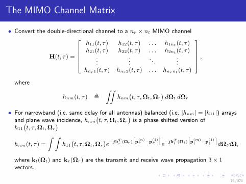
• Convert the double-directional channel to a nr × nt MIMO channel
H(t, τ ) =
h11(t, τ ) h12(t, τ ) . . . h1nt(t, τ )h21(t, τ ) h22(t, τ ) . . . h2nt(t, τ )
......
. . ....
hnr1(t, τ ) hnr2(t, τ ) . . . hnrnt(t, τ )
,
where
hnm(t, τ ) ,
∫∫
hnm
(t, τ,Ωt,Ωr
)dΩt dΩr
• For narrowband (i.e. same delay for all antennas) balanced (i.e. |hnm| = |h11|) arraysand plane wave incidence, hnm
(t, τ,Ωt,Ωr
)is a phase shifted version of
h11
(t, τ,Ωt,Ωr
)
hnm(t, τ ) =
∫ ∫
h11
(t, τ,Ωt,Ωr
)e−jkT
r (Ωr)[p(n)r −p
(1)r
]
e−jkTt (Ωt)
[p(m)t −p
(1)t
]
dΩtdΩr
where kt(Ωt) and kr(Ωr) are the transmit and receive wave propagation 3× 1vectors.
76 / 273

Steering Vectors
• For a transmit ULA oriented broadside to the link axis,
e−jkTt (Ωt)·
[p(m)t −p
(1)t
]
= e−j(m−1)ϕt(θt),
where ϕt (θt) = 2π(dt/λ) cos θt, and dt =∥∥p
(m)t − p
(m−1)t
∥∥ denotes the
inter-element spacing of the transmit array.– θt is defined relatively to the array orientation (so θt = π/2 corresponds to the link axis
for a broadside array).
• Steering vector (expressed here for a ULA)– At the transmitter in the relative direction θt:
at(θt) = [ 1 e−jϕt(θt) . . . e−j(nt−1)ϕt(θt) ]T .
– At the receiver in the relative direction θr :
ar (θr) = [ 1 e−jϕr(θr) . . . e−j(nr−1)ϕr(θr) ]T .
• Under the plane wave and balanced narrowband array assumptions, the MIMOchannel matrix can be rewritten as a function of steering vectors as
H(t, τ ) =
∫ ∫
h(t,p
(1)t ,p(1)
r , τ,Ωt,Ωr
)ar(Ωr) a
Tt (Ωt) dΩt dΩr.
77 / 273

A Finite Scatterer MIMO Channel Representation
• The transmitter and receiver are coupled via a finite number of scattering paths withns,t DoDs at the transmitter and ns,r DoAs at the receiver.−→ Replace the integral by a summation (assume for simplicity 2-D azimuthalpropagation)
H(t, τ ) =
ns,t∑
l=1
ns,r∑
p=1
h(l,p)11 (t, τ )ar(θ
(p)r )aT
t (θ(l)t )
= ArHs(t, τ )ATt
where– Ar and At represent the nr × ns,r and nt × ns,t matrices whose columns are the
steering vectors related to the directions of each path observed at Rx and Tx– Hs(t, τ) is a ns,r × ns,t matrix whose elements are the complex path gains between all
DoDs and DoAs at time instant t and delay τ
• Assume the columns of At are written as at(θ(l)t ), l = 1, ..., ns,t. Let us write
H = ArHs︸ ︷︷ ︸
Hs
ATt =
ns,t∑
l=1
Hs(:, l)aTt (θ
(l)t ) =
ns,t∑
l=1
H(l),
where H(l) can be viewed as the channel matrix corresponding to the lth scattererlocated in the direction of departure θ
(l)t .
78 / 273

Statistical Properties of the MIMO Channel Matrix
• Assume narrowband channels, the spatial correlation matrix of the MIMO channel
R = Evec(HH)vec(HH)H
This is a ntnr × ntnr positive semi-definite Hermitian matrix.• It describes the correlation between all pairs of transmit-receive channels:
– E H(n,m)H∗(n,m): the average energy of the channel between antenna m andantenna n,
– r(nq)m = E H(n,m)H∗(q,m): the receive correlation between channels originatingfrom transmit antenna m and impinging upon receive antennas n and q,
– t(mp)n = E H(n,m)H∗(n, p): the transmit correlation between channels originatingfrom transmit antennas m and p and arriving at receive antenna n,
– E H(n,m)H∗(q, p): the cross-channel correlation between channels (m,n) and(q, p).
Example
2x2 MIMO
R =
1 t∗1 r∗1 s∗1t1 1 s∗2 r∗2r1 s2 1 t∗2s1 r2 t2 1
t1 = E H(1, 1)H∗(1, 2)r1 = E H(1, 1)H∗(2, 1)
79 / 273

Spatial Correlation
• How are these correlations related to the propagation channel?• Let us consider the case of ULAs and 2-D azimuthal propagation
hnm(t) =
∫ ∫
h11
(t,Ωt,Ωr
)e−j(m−1)ϕt(θt) e−j(n−1)ϕr(θr) dθt dθr
where– ϕr,t (θr,t) = 2π(dr,t/λ) cos θr,t,– dr and dt are the inter-element spacing at the receive/transmit arrays
– h11(t,Ωt,Ωr
),∫h11(t, τ,Ωt,Ωr
)dτ .
• Correlation between channels hnm and hqp
Ehnmh∗
qp
= E
∫ 2π
0
∫ 2π
0
∣∣h11
(t,Ωt,Ωr
)∣∣2 e−j(m−p)ϕt(θt) e−j(n−q)ϕr(θr) dθt dθr
=
∫ 2π
0
∫ 2π
0
E∣∣h11
(t,Ωt,Ωr
)∣∣2
e−j(m−p)ϕt(θt) e−j(n−q)ϕr(θr) dθt dθr,
=
∫ 2π
0
∫ 2π
0
A (θt, θr) e−j(m−p)ϕt(θt) e−j(n−q)ϕr(θr) dθt dθr,
where A (θt, θr) is the joint direction power spectrum restricted to the azimuthangles.
• The channel correlation is related to both the antenna spacings and the jointdirection power spectrum!
80 / 273

Spatial Correlation
• When the energy spreading is very large at both sides and dt/dr are sufficientlylarge, elements of H become uncorrelated, and R becomes diagonal.
Example
Consider two transmit antennas spaced by dt. The transmit correlation writesas
t =
∫ 2π
0
ej2π(dt/λ) cos θtAt(θt)dθt,
which only depends on the transmit antenna spacing and the transmit directionpower spectrum.
– isotropic scattering : very rich scattering environment around the transmitter witha uniform distribution of the energy, i.e. At(θt) ∼= 1/2π
t =1
2π
∫ 2π
0ejϕt(θt)dθt =
1
2π
∫ 2π
0ej2π(dt/λ) cos θtdθt
= J0
(
2πdt
λ
)
.
The transmit correlation only depends on the spacing between the two antennas.
81 / 273

Spatial Correlation
Example
– highly directional scattering : scatterers around the transmit array areconcentrated along a narrow direction θt,0, i.e., At(θt)→ δ(θt − θt,0)
t→ ejϕt(θt,0) = ej2π(dt/λ) cos θt,0 .
Very high transmit correlation approaching one. The scattering direction isdirectly related to the phase of the transmit correlation.
0 0.5 1 1.5 2 2.5 3 3.5 4−0.5
0
0.5
1
Transmit antenna spacing relative to wavelength
Tra
nsm
it co
rrel
atio
n
κ = 0
κ = 10
κ = 100
κ = 500
κ = 2
– At(θt) in real-world channels:neither uniform nor a delta.
– isotropic scattering (κ = 0): firstminimum for dt = 0.38λ
– directional scattering (κ =∞):correlation never reaches 0
– in practice, decorrelation in richscattering is reached fordt ≈ 0.5λ
– The more directional theazimuthal dispersion (i.e. for κincreasing), the larger theantenna spacing required toobtain a null correlation.
82 / 273

Analytical Representation of Rayleigh MIMO Channels
• Independent and Identically Distributed (I.I.D.) Rayleigh fading– R = Intnr
– H = Hw is a random fading matrix with unit variance and i.i.d. circularly symmetriccomplex Gaussian entries.
• Realistic in practice only if both conditions are satisfied:– the antenna spacings and/or the angle spreads at Tx and Rx are large enough,– all individual channels characterized by the same average power (i.e., balanced array).
• What about real-world channels? Sometimes significantly deviate from this idealchannel:
– limited angular spread and/or reducedarray sizes cause the channels to becomecorrelated (channels are not independentanymore)
– a coherent contribution may induce thechannel statistics to become Ricean(channels are not Rayleigh distributedanymore),
– the use of multiple polarizations createsgain imbalances between the variouselements of the channel matrix (channelsare not identically distributed anymore).
83 / 273

Correlated Rayleigh Fading Channels
• For identically distributed Gaussian channels, R constitutes a sufficient description ofthe stochastic behavior of the MIMO channel.
• Any channel realization is obtained by
vec(H
H) = R1/2 vec(Hw),
where Hw is one realization of an i.i.d. channel matrix.• Complicated to use because
– cross-channel correlation not intuitive and not easily tractable– Too many parameters: dimensions of R rapidly become large as the array sizes increase– vec operation complicated for performance analysis
• Kronecker model: use a separability assumption
R = Rr ⊗Rt,
H = R1/2r HwR
1/2t
where Rt and Rr are respectively the transmit and receive correlation matrices.• Strictly valid only if r1 = r2 = r and t1 = t2 = t and s1 = rt and s2 = rt∗ (for 2× 2)
R =
1 t∗1 r∗1 s∗1t1 1 s∗2 r∗2r1 s2 1 t∗2s1 r2 t2 1
=
1 t∗ r∗ r∗t∗
t 1 r∗t r∗
r rt∗ 1 t∗
rt r t 1
=
[1 r∗
r 1
]
︸ ︷︷ ︸
Rr
⊗[
1 t∗
t 1
]
︸ ︷︷ ︸
Rt
84 / 273

Correlated Rayleigh Fading Channels
Example
Question: Assume a MISO system with two transmit antennas. The channelgains are identically distributed circularly symmetric complex Gaussian but canbe correlated and are denoted as h1 and h2. Write the expression of thetransmit correlation matrix Rt and derive the eigenvalues and eigenvectors ofRt as a fonction of the transmit correlation coefficient t.Answer: We write
Rt = E[
h∗1
h∗2
][h1 h2
]
=
[E|h1|2
E h∗
1h2E h1h
∗2 E
|h2|2
]
=
[1 t∗
t 1
]
where t = E h1h∗2 is the transmit correlation coefficient. The SVD leads to
Rt =
[1 1
t/|t| −t/|t|
] [1 + |t| 0
0 1− |t|
] [1 1
t/|t| −t/|t|
]H
.
The eigenvalues are only function of the magnitude of t while the eigenvectorsare only function of the phase of t.
85 / 273

Correlated Rayleigh Fading Channels
Example
Question: Assume the previous example with |t| → 1. Compute the weights ofthe matched beamformer (or maximum ratio transmission/transmit MRC).Answer: With matched beamforming, w = hH/ ‖h‖ where
h = hwR1/2t
= hw
[1 1
t/|t| −t/|t|
] [ √1 + |t| 0
0√
1− |t|
] [1 1
t/|t| −t/|t|
]H
= 2hw
[1
t/|t|
] [1
t/|t|
]H
where the last equality comes from the fact that |t| = 1. This shows that forhigh correlation, the channel direction (h/ ‖h‖) is aligned with
[1 t∗/|t|
].
Hence
w = hH/ ‖h‖ =
[1
t/|t|
]
.
Transmission is performed in the direction where all scatterers are located.
86 / 273
MIMO - An Interpretation using Radiation Patterns
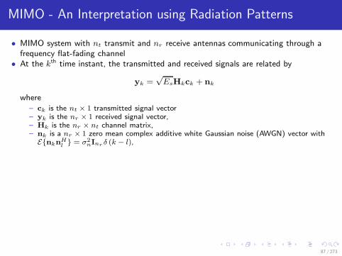
• MIMO system with nt transmit and nr receive antennas communicating through afrequency flat-fading channel
• At the kth time instant, the transmitted and received signals are related by
yk =√EsHkck + nk
where– ck is the nt × 1 transmitted signal vector– yk is the nr × 1 received signal vector,– Hk is the nr × nt channel matrix,– nk is a nr × 1 zero mean complex additive white Gaussian noise (AWGN) vector withEnkn
Hl = σ2nInr δ (k − l),
87 / 273

Radiation Patterns
• Decompose the channel Hk =∑L−1
l=0 H(l)k =
∑L−1l=0 H
(l)k (:, 1) aT
t
(θ(l)t,k
), where
at
(θ(l)t,k
)is the transmit array response in the direction of departure θ
(l)t,k.
• Hence,
Hkck =L−1∑
l=0
H(l)k (:, 1)aT
t
(θ(l)t,k
)ck
• The original MIMO transmission can be considered as the SIMO transmission of anequivalent codeword, given at the kth time instant by
aTt ck
• It may be thought of as an array factor function of the transmitted codewords. Atevery symbol period,
– the energy radiated in any direction varies as a function of the transmitted codewords.– for a given codeword and omnidirectional antennas, the radiated energy is not uniformly
distributed in all directions, but may present maxima and minima in certain directions.
88 / 273

Radiation Patterns
89 / 273

Radiation Patterns
Example
nt = 2: ck = [ c1 [k] c2 [k] ]T
cTk at (θt) = c1 [k]
[
1 +c2 [k]
c1 [k]e−2πj
dtλ
cos θt
]
︸ ︷︷ ︸
Gt(θt |ck)
1
2
30
210
60
240
90
270
120
300
150
330
180 0
0 phase shift
1
2
30
210
60
240
90
270
120
300
150
330
180 0
π/2 phase shift
1
2
30
210
60
240
90
270
120
300
150
330
180 0
π phase shift
1
2
30
210
60
240
90
270
120
300
150
330
180 0
3π/2 phase shift
−2 −1 0 1 2 3 410
−2
10−1
100
Phase shift between the two transmitted symbols [rad]
SE
R
d/λ=0.5
d/λ=0.1
90 / 273

Capacity of point-to-point MIMO Channels
91 / 273

Reference Book
• Bruno Clerckx and Claude Oestges, “MIMO Wireless Networks: Channels,Techniques and Standards for Multi-Antenna, Multi-User and Multi-Cell Systems,”Academic Press (Elsevier), Oxford, UK, Jan 2013.
– Chapter 5
Section: 5.1, 5.2, 5.3, 5.4.1, 5.4.2(except “Antenna Selection Schemes”),5.5.1 - “Kronecker Correlated RayleighChannels”, 5.5.2, 5.7, 5.8.1 (exceptProof of Proposition 5.9 and Example5.4)
92 / 273

Introduction - Previous Lectures
• Transmission strategies– Space-Time Coding when no Tx channel knowledge– Multiple (including dominant) eigenmode transmission when Tx channel knowledge
z =√
EsGHc′ +Gn
=√
EsUHHHVHc+UHn
=√
EsΣHc+ n.
Multiple parallel data pipes → Spatial multiplexing gain!
• Performance highly depends on the channel matrix properties– Angle spread and inter-element spacing– Spatial Correlation: spread antennas far apart to decrease spatial correlation– Rayleigh and Ricean distribution
93 / 273
System Model
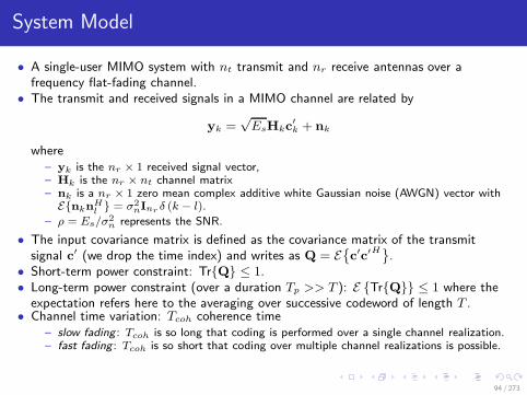
• A single-user MIMO system with nt transmit and nr receive antennas over afrequency flat-fading channel.
• The transmit and received signals in a MIMO channel are related by
yk =√EsHkc
′k + nk
where– yk is the nr × 1 received signal vector,– Hk is the nr × nt channel matrix– nk is a nr × 1 zero mean complex additive white Gaussian noise (AWGN) vector withEnkn
Hl = σ2nInr δ (k − l).
– ρ = Es/σ2n represents the SNR.
• The input covariance matrix is defined as the covariance matrix of the transmitsignal c′ (we drop the time index) and writes as Q = E
c′c′
H.
• Short-term power constraint: TrQ ≤ 1.• Long-term power constraint (over a duration Tp >> T ): E TrQ ≤ 1 where the
expectation refers here to the averaging over successive codeword of length T .• Channel time variation: Tcoh coherence time
– slow fading : Tcoh is so long that coding is performed over a single channel realization.– fast fading : Tcoh is so short that coding over multiple channel realizations is possible.
94 / 273

Capacity of Deterministic MIMO Channels
Proposition
For a deterministic MIMO channel H, the mutual information I is written as
I(H,Q) = log2 det
[
Inr + ρHQHH
]
where Q is the input covariance matrix whose trace is normalized to unity.
Definition
The capacity of a deterministic nr × nt MIMO channel with perfect channelstate information at the transmitter is
C (H) = maxQ≥0:TrQ=1
log2 det
[
Inr + ρHQHH
]
.
Note the difference with SISO capacity.
95 / 273

Capacity and Water-Filling Algorithm
• What is the best transmission strategy, i.e. the optimum input covariance matrix Q?• First, create n = minnt, nr parallel data pipes (Multiple Eigenmode Transmission)
– Decouple the channel along the individual channel modes (in the directions of thesingular vectors of the channel matrix H at both the transmitter and the receiver)
H = UHΣHVHH ,
UHHHVH = UH
HUHΣHVHHVH = ΣH
– Optimum input covariance matrix Q⋆ writes as
Q⋆ = VHdiag s⋆1, . . . , s⋆nVHH ,
• Second, allocate power to data pipes– ΣH = diag σ1, . . . , σn, and σ2k , λk– Capacity: C(H) = maxsknk=1
∑nk=1 log2
[1 + ρskλk
]=∑n
k=1 log2[1 + ρs⋆kλk
]
Proposition
The power allocation strategy s1, . . . , sn = s⋆1, . . . , s⋆n that maximizes∑n
k=1 log2 (1 + ρλksk) under the power constraint∑n
k=1 sk = 1, is given by thewater-filling solution,
s⋆k =
(
µ− 1
ρλk
)+
, k = 1, . . . , n
where µ is chosen so as to satisfy the power constraint∑n
k=1 s⋆k = 1.
96 / 273

Water-Filling Algorithm
• Iterative power allocation
– Order eigenvalues λk in decreasing orderof magnitude
– At iteration i, evaluate the constant µfrom the power constraint
µ(i) =1
n− i+ 1
(
1 +
n−i+1∑
k=1
1
ρλk
)
– Calculate power
sk(i) = µ(i) − 1
ρλk,
k = 1, . . . , n− i+ 1.
If sn−i+1 < 0, set to 0
– Iterate till the power allocated on eachmode is non negative.
∗
1s
∗
2s
∗
3s
. . .
1
1
ρ λ2
1
ρ λ
3
1
ρ λ
1
1
-nρ λ
nρ λ
1
µ
97 / 273

Water-Filling Algorithm
Example
Question: Consider the transmission y = Hc′ + n with perfect CSIT over adeterministic point to point MIMO channel whose matrix is given by
H =
[a 0 a 00 b 0 b
]
where a and b are complex scalars with |a| ≥ |b|. The input covariance matrixis given by Q = E
c′c′H
and is subject to the transmit power constraint
Tr Q ≤ P .1 Compute the capacity with perfect CSIT of that deterministic channel.Particularize to the case a = b. Explain your reasoning.
2 Explain how to achieve that capacity.
3 In which deployment scenario, could such channel matrix structure beencountered?
98 / 273

Water-Filling Algorithm
Example
Answer:1 Let us write Q = VPVH with the diagonal element of P, denoted as Pk
(satisfying∑nt
k=1 Pk = P ), refers to the power allocated to stream k. Thecapacity with perfect CSIT over the deterministic channel H is given by
C (H) = maxP1,...,Pk
min2,4∑
k=1
log2
(
1 +Pk
σ2n
λk
)
where λk refers the non-zero eigenvalue of HHH, respectively equal to2 |a|2 and 2 |b|2. Hence,
C (H) = maxP1,P2
(
log2
(
1 +P1
σ2n
2 |a|2)
+ log2
(
1 +P2
σ2n
2 |b|2))
.
The optimal power allocation is given by the water-filling solution
P ⋆1 =
(
µ− σ2n
2 |a|2)+
, P ⋆2 =
(
µ− σ2n
2 |b|2)+
with µ computed such that P ⋆1 + P ⋆
2 = P .
99 / 273

Water-Filling Algorithm
Example
Answer:Assuming P ⋆
1 and P ⋆2 are positive, µ = P
2+
σ2n
4
(1
|a|2 + 1|b|2
)
. If µ− σ2n
2|b|2 ≤ 0,
i.e. P2+
σ2n
4|a|2 −σ2n
4|b|2 ≤ 0, P ⋆2 = 0 and P ⋆
1 = P . The capacity writes as
C (H) = log2
(
1 +P
σ2n
2 |a|2)
.
If P2+
σ2n
4|a|2 −σ2n
4|b|2 > 0, P ⋆1 = P
2− σ2
n
4|a|2 +σ2n
4|b|2 and P ⋆2 = P
2+
σ2n
4|a|2 −σ2n
4|b|2 .
The capacity writes as
C (H) = log2
(
1 +P ⋆1
σ2n
2 |a|2)
+ log2
(
1 +P ⋆2
σ2n
2 |b|2)
.
In the particular case where a = b, uniform power allocation P ⋆1 = P ⋆
2 = P2
isoptimal and
C (H) = 2 log2
(
1 +P
σ2n
|a|2)
.
100 / 273

Water-Filling Algorithm
Example
Answer:2 Transmit along V, given by the two dominant eigenvector of HHH. Theyare easily computed given the orthogonality of the channel matrix H as
V =1√2
1 00 11 00 1
.
The power allocated to the two streams is given by P ⋆1 and P ⋆
2 . At thereceiver, the precoded channel is already decoupled and no furthercombiner is necessary. Each stream can be decoded using thecorresponding SISO decoder.
3 Dual-polarized antenna deployment (e.g. VHVH-VH) with LoS and goodantenna XPD.
101 / 273

Capacity Bounds and Suboptimal Power Allocations
• Low SNR: power allocated to the dominant eigenmode
C (H)ρ→0→ log2 (1 + ρλmax) .
• High SNR: power is uniformly allocated among the non-zero modes
C (H)ρ→∞→
n∑
k=1
log2
(
1 +ρ
nλk
)
.
• At any SNR– lower bound
C (H) ≥ log2 (1 + ρλmax) ,
C (H) ≥n∑
k=1
log2
(
1 +ρ
nλk
)
.
– upper bound (use Jensen’s inequality Ex F (x) ≤ F (Ex x) if F concave)
CCSIT (H) =n∑
k=1
log2[1 + ρs⋆kλk
] (a)
≤ n log2
(
1 +ρ
n
[n∑
k=1
s⋆kλk
])
,
≤ n log2
[
1 +ρ
nλmax
]
.
102 / 273

Ergodic Capacity of Fast Fading Channels
• Fast fading:– Doppler frequency sufficiently high to allow for coding over many channel
realizations/coherence time periods– The transmission capability is represented by a single quantity known as the ergodic
capacity
• MIMO Capacity with Perfect Transmit Channel Knowledge– similar strategy as in deterministic channels: transmit along eigenvectors of channel
matrix and allocate power following water-filling– short term power constraint: water-filling solution applied over space as in
deterministic channels
CCSIT,ST = E
maxQ≥0:TrQ=1
log2 det
[
Inr + ρHQHH
]
=n∑
k=1
E
log2[1 + ρs⋆kλk
]
.
– Impact on coding strategy? Use a variable-rate code (family of codes of different rates)adapted as a function of the water-filling allocation. No need for the codeword to spanmany coherence time periods.
103 / 273

MIMO Capacity with Partial Transmit Channel Knowledge
• H is not known to the transmitter → we cannot adapt Q at all time instants• Rate of information flow between Tx and Rx at time instant k over channels Hk
log2 det[
Inr + ρHkQHHk
]
.
Such a rate varies over time according to the channel fluctuations. The average rateof information flow over a time duration T >> Tcoh is
1
T
T−1∑
k=0
log2 det[
Inr + ρHkQHHk
]
.
Definition
The ergodic capacity of a nr × nt MIMO channel with channel distributioninformation at the transmitter (CDIT) is given by
CCDIT , C = maxQ≥0:TrQ=1
E
log2 det[
Inr + ρHQHH]
,
where Q is the input covariance matrix optimized as to maximize the ergodicmutual information.
• T >> Tc to average out the noise and the channel fluctuations104 / 273

I.I.D. Rayleigh Fast Fading Channels: Perfect TransmitChannel Knowledge
• Low SNR: allocate all the available power to the strongest or dominant eigenmode.Use log2(1 + x) ≈ x log2 (e) for x small and get
CCSIT,ST = E
log2[1 + ρλmax
]
∼= ρEλmax
log2(e)
∼= ρn log2(e), N, n→∞, N/n >> 0.
CCSIT,LT = E
log2[1 + ρs⋆maxλmax
]
∼= ρEs⋆maxλmax
log2(e)
Observations: CCSIT grows linearly in the minimum number of antennas n.• High SNR: uniform power allocation on all non-zeros eigenmodes
CCSIT∼=
n∑
k=1
E
log2
[
1 +ρ
nλk
]
∼= nlog2
( ρ
n
)
+ E
n∑
k=1
log2(λk)
.
Observations: CCSIT also scales linearly with n. The spatial multiplexing gain isgs = n. MISO fading channels do not offer any multiplexing gain.
105 / 273

I.I.D. Rayleigh Fast Fading Channels: Partial TransmitChannel Knowledge
• Optimal covariance matrix
Proposition
In i.i.d. Rayleigh fading channels, the ergodic capacity with CDIT is achievedunder an equal power allocation scheme Q = Int/nt, i.e.,
CCDIT = Ie = E
log2 det
[
Inr +ρ
ntHwH
Hw
]
= E
n∑
k=1
log2
[
1 +ρ
ntλk
]
.
Encoding requires a fixed-rate code (whose rate is given by the ergodic capacity)with encoding spanning many channel realizations.
• Low SNR:
CCDIT ≥ E
log2
[
1 +ρ
nt‖Hw‖2F
]
≈ ρ
ntE‖Hw‖2F
log2 (e) = nrρ log2 (e)
Observations:– CCDIT is only determined by the energy of the channel.– A MIMO channel only yields a nr gain over a SISO channel. Increasing the number of
transmit antennas is not useful (contrary to perfect CSIT). SIMO and MIMO channelsreach the same capacity for a given nr .
106 / 273

I.I.D. Rayleigh Fast Fading Channels: Partial TransmitChannel Knowledge
• High SNR:
CCDIT ≈ E
n∑
k=1
log2
[ρ
ntλk
]
= nlog2
( ρ
nt
)
+ E
n∑
k=1
log2(λk)
Observations:– CCDIT at high SNR scales linearly with n (by contrast to the low SNR regime).– The multiplexing gain gs is equal to n, similarly to the CSIT case.– CCDIT and CCSIT are not equal: constant gap equal to n log2(nt/n) at high SNR.
• Expressions can be particularized to SISO, SIMO, MISO cases. At high SNR,– SISO (N = n = 1):
CCDIT ≈ log2(ρ) + E
log2
(
|h|2)
= log2(ρ) − 0.83 = CAWGN − 0.83
– SIMO (nt = n = 1, nr = N):
CCDIT ≈ log2(nrρ)
– MISO (nr = n = 1, nt = N):
CCDIT ≈ log2(ρ) + E
log2
(
‖h‖2 /nt
) nt→∞≈ log2(ρ) = CAWGN
107 / 273

I.I.D. Rayleigh Fast Fading Channels
• Ergodic capacity of various nr × nt i.i.d. Rayleigh channels with full (CSIT) andpartial (CDIT) channel knowledge at the transmitter.
−10 −5 0 5 10 15 200
2
4
6
8
10
12
14
16
18
20
SNR [dB]
Erg
odic
cap
acity
[bps
/Hz]
2 x 2 (CSIT)4 x 2 (CSIT)2 x 4 (CSIT)4 x 4 (CSIT)2 x 2 (CDIT)4 x 2 (CDIT)2 x 4 (CDIT)4 x 4 (CDIT)
108 / 273

I.I.D. Rayleigh Fast Fading Channels
Example
Question: Here is the ergodic capacity of point-to-point i.i.d. Rayleigh fastfading channels with Channel Distribution Information at the Transmitter(CDIT) for five antenna (nr × nt) configurations (denoted as (a) to (e)) withnt + nr = 8.
−10 −7 −4 −1 2 5 8 11 14 17 20 23 26 290
2
4
6
8
10
12
14
16
18
20
22
24
26
28
30
SNR [dB]
Erg
odic
cap
acity
[bits
/s/H
z]
(a)(b)(c)(d)(e)
109 / 273

I.I.D. Rayleigh Fast Fading Channels
Example
Question: What is the achievable (spatial) multiplexing gain (at high SNR) forcases (a), (b), (c), (d) and (e)? Provide your reasoning.
Answer: The multiplexing gain is the pre-log factor of the ergodic capacity athigh SNR, i.e. gs = limρ→∞
CCDIT
log2(ρ). Hence by increasing the SNR by 3dB
(e.g. from 17dB to 20dB), the ergodic capacity increases by gs bits/s/Hz.(a) gs = 3.
(b) gs = 2.
(c) gs = 2.
(d) gs = 1.
(e) gs = 1.
110 / 273

I.I.D. Rayleigh Fast Fading Channels
Example
Question: For (a), (b), (c), (d) and (e), identify an antenna configuration, i.e.nt and nr, satisfying nt + nr = 8 that achieves such multiplexing gain. Provideyour reasoning.
Answer: There are several possible configurations that satisfy to nr + nt = 8,namely 5× 3, 3× 5, 6× 2, 2× 6, 7× 1 and 1× 7, 4× 4. The matchingbetween curves and antenna configurations is easily identified by using thefollowing two arguments: 1) The multiplexing gain with CDIT at high SNR isgiven by min nt, nr. 2) With CDIT only, the input covariance matrix in i.i.d.channel is Q = 1/ntInt . This implies that 6× 2 and 7× 1 outperform 2× 6and 1× 7, respectively.(a) nr × nt = 5× 3 or 3× 5
(b) nr × nt = 6× 2
(c) nr × nt = 2× 6
(d) nr × nt = 7× 1
(e) nr × nt = 1× 7
111 / 273
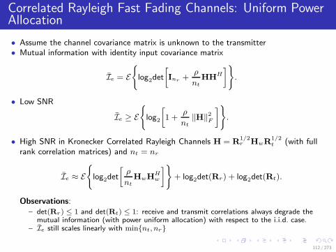
Correlated Rayleigh Fast Fading Channels: Uniform PowerAllocation
• Assume the channel covariance matrix is unknown to the transmitter• Mutual information with identity input covariance matrix
Ie = E
log2det
[
Inr +ρ
ntHH
H
]
.
• Low SNR
Ie ≥ E
log2
[
1 +ρ
nt‖H‖2F
]
.
• High SNR in Kronecker Correlated Rayleigh Channels H = R1/2r HwR
1/2t (with full
rank correlation matrices) and nt = nr
Ie ≈ E
log2det
[ρ
ntHwH
Hw
]
+ log2det(Rr) + log2det(Rt).
Observations:– det(Rr) ≤ 1 and det(Rt) ≤ 1: receive and transmit correlations always degrade the
mutual information (with power uniform allocation) with respect to the i.i.d. case.– Ie still scales linearly with minnt, nr
112 / 273
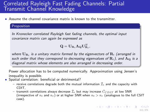
Correlated Rayleigh Fast Fading Channels: PartialTransmit Channel Knowledge
• Assume the channel covariance matrix is known to the transmitter.
Proposition
In Kronecker correlated Rayleigh fast fading channels, the optimal inputcovariance matrix can again be expressed as
Q = URtΛQUHRt
,
where URt is a unitary matrix formed by the eigenvectors of Rt (arranged insuch order that they correspond to decreasing eigenvalues of Rt), and ΛQ is adiagonal matrix whose elements are also arranged in decreasing order.
Power allocation has to be computed numerically. Approximation using Jensen’sinequality is possible.
• Spatial correlation: beneficial or detrimental?– receive correlations degrade both the mutual information Ie and the capacity with
CDIT,– transmit correlations always decrease Ie but may increase CCDIT at low SNR
(irrespective of nt and nr) or at higher SNR when nt > nr (analogous to the full CSITcase).
113 / 273

Correlated Rayleigh Fast Fading Channels: PartialTransmit Channel Knowledge
• Mutual information of various strategies at 0 dB SNR as a function of the transmitcorrelation |t| in TIMO. Beamforming refers here to the tranmsission of one streamalong the dominant eigenvector of Rt.
0 0.2 0.4 0.6 0.8 12.6
2.7
2.8
2.9
3
3.1
3.2
3.3
3.4
3.5
3.6
Magnitude of transmit correlation
Mu
tua
l in
form
atio
n/c
ap
acity [
bp
s/H
z]
Optimal allocationEqui−power allocationBeamforming
114 / 273

Outage Capacity and Probability in Slow Fading Channels
• In slow fading, the encoding still averages out the randomness of the noise butcannot fully average out the randomness of the channel.
• For a given channel realization H and a target rate R, reliable transmission if
log2 det(
Inr + ρHQHH)
> R
If not met with any Q, an outage occurs and the decoding error probability is strictlynon-zero.
• Look at the tail probability of log2 det(Inr + ρHQHH
), not its average!
Definition
The outage probability Pout (R) of a nr × nt MIMO channel with a target rateR is given by
Pout (R) = minQ≥0:TrQ≤1
P(
log2 det(
Inr + ρHQHH)
< R)
,
where Q is the input covariance matrix optimized as to minimize the outageprobability.
• More meaningful in the absence of CSI knowledge at the transmitter: the transmittercannot adjust its transmit strategy → hopes the channel is good enough
115 / 273

Diversity-Multiplexing Trade-Off in Slow Fading Channels
• For a given R, how does Pout behave as a function of the SNR ρ?
Definition
A diversity gain g⋆d (gs,∞) is achieved at multiplexing gain gs at infinite SNR if
limρ−→∞
R(ρ)
log2(ρ) = gs
limρ−→∞
log2(Pout (R)
)
log2
(ρ) = −g⋆d (gs,∞)
The curve g⋆d (gs,∞) as function of gs is known as the asymptoticdiversity-multiplexing trade-off of the channel.
– The multiplexing gain indicates how fast the transmission rate increases with the SNR.– The diversity gain represents how fast the outage probability decays with the SNR.
116 / 273

Diversity-Multiplexing Trade-Off in I.I.D. Rayleigh SlowFading Channels
• Point (0, ntnr): for a spatialmultiplexing gain of zero (i.e., R isfixed), the maximal diversity gainachievable is ntnr.
• Point (min nt, nr , 0):transmitting at diversity gain g⋆d = 0(i.e., Pout is kept fixed) allows thedata rate to increase with SNR asn = min nt, nr.• Intermediate points: possible to
transmit at non-zero diversity andmultiplexing gains but that anyincrease of one of those quantitiesleads to a decrease of the otherquantity.
Spatial multiplexing gain g
Div
ers
ity g
ain
g *
(g ,
)
(0,ntnr)
(1,(nt−1)(nr−1))
(2,(nt−2)(nr−2))
(g , (n − g )(n − g )) r
(min(nt,nr),0)
ds
s
s sst
∞
117 / 273

Diversity-Multiplexing Trade-Off in I.I.D. Rayleigh SlowFading Channels
• For fixed rates R = 2, 4, ..., 40bits/s/Hz,
– The asymptotic slope of eachcurve is four and matches themaximum diversity gain g⋆d (0,∞).
– The horizontal separation is 2bits/s/Hz per 3 dB, whichcorresponds to the maximummultiplexing gain equal to n(= 2).
• As the rate increases more rapidlywith SNR (i.e., as the multiplexinggain gs increases), the slope of theoutage probability curve (given bythe diversity gain g∗d) vanishes.
0 10 20 30 40 50 6010
−5
10−4
10−3
10−2
10−1
100
SNR [dB]
Ou
tag
e p
rob
ab
ility
Po
ut
g =1.75g =0.25
g =1.5
g =0.5
g =1.25
g =0.75
g =1.0g =1.0
g =0.75g =1.75g =0.5
g =2.5
s
d*
s
s
s
s
s
*
*
*
*
*
d
d
d
d
d
Figure: 2× 2 MIMO i.i.d. Rayleigh fading channels
118 / 273

Diversity-Multiplexing Trade-Off of a Scalar RayleighChannel h
• Determine for a transmission rate R scaling with ρ as gs log2 (ρ), the rate at whichthe outage probability decreases with ρ as ρ increases.
• Outage probability
Pout (R) = P(log2
[1 + ρ |h|2
]< gs log2 (ρ)
)
= P(1 + ρ |h|2 < ρgs
)
• At high SNR,
Pout (R) ≈ P(
|h|2 ≤ ρ−(1−gs))
• Since |h|2 is exponentially distributed, i.e., P(|h|2 ≤ ǫ
)≈ ǫ for small ǫ
Pout (R) ≈ ρ−(1−gs)
An outage occurs at high SNR when |h|2 ≤ ρ−(1−gs) with a probability ρ−(1−gs).• DMT for the scalar Rayleigh fading channel g⋆d (gs,∞) = 1− gs for gs ∈ [0, 1].
119 / 273

Space-Time Coding over I.I.D. Rayleigh Flat
Fading Channels
120 / 273

Reference Book
• Bruno Clerckx and Claude Oestges, “MIMO Wireless Networks: Channels,Techniques and Standards for Multi-Antenna, Multi-User and Multi-Cell Systems,”Academic Press (Elsevier), Oxford, UK, Jan 2013.
– Chapter 6
Section: 6.1, 6.2, 6.3 (except “AntennaSelection” in 6.3.2), 6.4.1, 6.4.2 (exceptthe Proofs), 6.5.1, 6.5.2, 6.5.3, 6.5.4,6.5.8, Figure 7.1
121 / 273

Introduction - Previous Lectures
• Previous lecture– Capacity of deterministic MIMO channels
C (H) = maxQ≥0:TrQ=1
log2 det
[
Inr + ρHQHH
]
.
– Ergodic capacity of fast fading channels– Outage capacity and probability of slow fading channels
• MIMO provides huge gains in terms of reliability and transmission rate– diversity gain, array gain, coding gain, spatial multiplexing gain, interference
management
• What we further need– practical methodologies to achieve these gains?– how to code across space and time?– Some preliminary answers: multimode eigenmode transmission when channel knowledge
available at the Tx, Alamouti scheme when no channel knowledge available at the Tx
122 / 273

Overview of a Space-Time Encoder
• Space-time encoder: sequence of two black boxes
bits
space-time encoder
nt
codewordC
T
nt
temporal coding
symbol mapping
time interleavingsymbolsQB
space-time
coding
• First black box: combat the randomness created by the noise at the receiver.• Second black box: spatial interleaver which spreads symbols over several antennas in
order to mitigate the spatial selective fading.• The ratio B/T is the signaling rate of the transmission.• The ratio Q/T is defined as the spatial multiplexing rate (representative of how
many symbols are packed within a codeword per unit of time).
123 / 273

System Model
• MIMO system with nt transmit and nr receive antennas over a frequency flat-fadingchannel
• Transmit a codeword C = [c0 . . . cT−1] [nt × T ] contained in the codebook C• At the kth time instant, the transmitted and received signals are related by
yk =√EsHkck + nk
where– yk is the nr × 1 received signal vector,– Hk is the nr × nt channel matrix,– nk is a nr × 1 zero mean complex AWGN vector with Enkn
Hl = σ2nInr δ (k − l),
– The parameter Es is the energy normalization factor. SNR ρ = Es/σ2n.
• No transmit channel knowledge but we know it is i.i.d. Rayleigh fading.• Codeword average transmit power E
TrCCH
= T . Assume
E‖H‖2F
= ntnr.
• Channel time variation:– slow fading : Tcoh >> T and Hk = HwT−1
k=0 , with Hw denoting an i.i.d. randomfading matrix with unit variance circularly symmetric complex Gaussian entries.
– fast fading : T ≥ Tcoh and Hk = Hk,w, whereHk,w
T−1
k=0are uncorrelated matrices,
eachHk,w
being an i.i.d. random fading matrix with unit variance circularly
symmetric complex Gaussian entries.
124 / 273

Error Probability Motivated Design Methodology
• With instantaneous channel realizations perfectly known at the receive side, the MLdecoder computes an estimate of the transmitted codeword according to
C = argminC
T−1∑
k=0
∥∥∥yk −
√EsHkck
∥∥∥
2
where the minimization is performed over all possible codeword vectors C.• Pairwise Error Probability (PEP): probability that the ML decoder decodes the
codeword E = [e0 . . . eT−1] instead of the transmitted codeword C.• When the PEP is conditioned on the channel realizations HkT−1
k=0 , it is defined asthe conditional PEP,
P(
C→ E| HkT−1k=0
)
= Q
√√√√ρ
2
T−1∑
k=0
‖Hk (ck − ek)‖2F
where Q (x) is the Gaussian Q-function.• The average PEP, P (C→ E), obtained by averaging the conditional PEP over the
probability distribution of the channel gains.• System performance dominated at high SNR by the couples of codewords that lead
to the worst PEP.125 / 273

• Assume a fixed rate transmission, i.e., spatial multiplexing gain gs = 0.
Definition
The diversity gain god (ρ) achieved by a pair of codewords C,E ∈ C isdefined as the slope of P (C→ E) as a function of the SNR ρ on a log-logscale, usually evaluated at very high SNR, i.e.,
god(∞) = limρ→∞
god(ρ) = − limρ→∞
log2 (P (C→ E))
log2 ρ.
PS: god(∞)↔ P (C→ E) , g⋆d (0,∞)↔ Pout.
Definition
The coding gain achieved by a pair of codewords C,E ∈ C is defined as themagnitude of the left shift of the P (C→ E) vs. ρ curve evaluated at veryhigh SNR.
• If P (C→ E) is well approximated at high SNR by
P (C→ E) ≈ c (gcρ)−god(∞)
with c being a constant, gc is identified as the coding gain.126 / 273

Derivation of the Average PEP
• Conditional PEP
P(
C→ E| HkT−1k=0
)
= Q
√√√√ρ
2
T−1∑
k=0
‖Hk (ck − ek)‖2F
where Q (x) is the Gaussian Q-function defined as
Q (x)∆= P (y ≥ x) =
1√2π
∫ ∞
x
exp
(
−y2
2
)
dy.
• Average PEP
P (C→ E) = EHk
P(
C→ E| HkT−1k=0
)
.
• This integration is sometimes difficult to calculate. Therefore, alternatives forms ofthe Gaussian Q-function are used.
– Craig’s formula
Q (x) =1
π
∫ π/2
0exp
(
− x2
2 sin2 (β)
)
dβ.
– Chernoff bound
Q (x) ≤ exp
(
−x2
2
)
.
127 / 273

• We can derive the average PEP as follows
P (C→ E) = EHk
P(
C→ E| HkT−1k=0
)
=1
π
∫ π/2
0
MΓ
(
− 1
2 sin2 (β)
)
dβ
≤ MΓ
(
−1
2
)
with MΓ (γ) moment generating function (MGF) of Γ = ρ2
∑T−1k=0 ‖Hk (ck − ek)‖2F
MΓ (γ)∆=
∫ ∞
0
exp (γΓ) pΓ (Γ) dΓ
Theorem
The moment generating function of a Hermitian quadratic form in complexGaussian random variable y = zFzH , where z is a circularly symmetric complexGaussian vector with mean z and a covariance matrix Rz and F a Hermitianmatrix, is given by
My (s)∆=
∫ ∞
0
exp (sy) py (y) dy =exp
(szF (I− sRzF)
−1zH)
det (I− sRzF) 128 / 273

Fast Fading MIMO Channels
• Defining
H =[H1 H2 · · · HT
]
D = diag c1 − e1, c2 − e2, . . . , cT − eT ,we may write
T∑
k=1
‖Hk (ck − ek)‖2F = ‖HD‖2F = Tr
HDDHH
H
= vec(
HH)H
∆ vec(
HH)
where ∆ = Inr ⊗DDH . This is a hermitian quadratic form of complex Gaussian
random variables of the form zFzH (with z = vec(HH
)Hand F = ∆).
• We can use Theorem where the mean z = 0 is the zero vector and the covariancematrix is Rz = E
vec(HH
)vec(HH
)H= ITnrnt (for i.i.d. channels).
• PEP averaged over i.i.d. Rayleigh fast fading channel (with η = ρ/(4 sin2 β))
P (C→ E) =1
π
∫ π/2
0
(det (ITnrnt + ηRz∆))−1 dβ
=1
π
∫ π/2
0
(
det(
ITnt + ηDDH))−nr
dβ
=1
π
∫ π/2
0
(
det(
IT + ηDHD))−nr
dβ.129 / 273

• In i.i.d. Rayleigh fast fading channels, average PEP reads as
P (C→ E) =1
π
∫ π/2
0
T−1∏
k=0
(1 + η ‖ck − ek‖2
)−nrdβ
where η = ρ/(4 sin2 β).• Upper bound using the Chernoff bound
P (C→ E) ≤T−1∏
k=0
(
1 +ρ
4‖ck − ek‖2
)−nr
.
• In the high SNR regime, the average PEP is further upper-bounded by
P (C→ E) ≤(ρ
4
)−nr lC,E ∏
k∈τC,E
‖ck − ek‖−2nr
with lC,E the effective length of the pair of codewords C,E, i.e., lC,E = ♯τC,E
with τC,E = k | ck − ek 6= 0.• Diversity gain: nrlC,E, coding gain:
∏
k∈τC,E‖ck − ek‖−2nr .
130 / 273

The Distance-Product Criterion
• At high SNR, the error probability is naturally dominated by the worst-case PEP
Design Criterion
(Distance-product criterion) Over i.i.d. Rayleigh fast fading channels,
1 distance criterion: maximize the minimum effective length Lmin of the codeover all pairs of codewords C,E with C 6= E
Lmin = minC,EC 6=E
lC,E
2 product criterion: maximize the minimum product distance dp of the code overall pairs of codewords C,E with C 6= E
dp = minC,EC 6=E
lC,E=Lmin
∏
k∈τC,E
‖ck − ek‖2
• The presence of multiple antennas at the transmitter does not impact the achievablediversity gain god (∞) = nrLmin but improves the coding gain gc = dp.
• The diversity gain is maximized first, and the coding gain is maximized only in asecond step.
131 / 273

Slow Fading MIMO Channels
• The conditional PEP writes as
P (C→ E |H) = Q(√
ρ
2‖H (C−E)‖2F
)
.
• The average PEP over Rayleigh slow fading channels is
P (C→ E) = EH P (C→ E|H) = 1
π
∫ π/2
0
MΓ
(
− 1
2 sin2 (β)
)
dβ
where MΓ (γ) moment generating function (MGF) of Γ = ρ2‖H (C−E)‖2F .
• Note that
‖H (C−E)‖2F = Tr
HEHH
= vec(
HH)H (
Inr ⊗ E)
vec(
HH)
where E = (C−E) (C−E)H .• This is a hermitian quadratic form of complex gaussian random variables of the form
zFzH (with z = vec(HH
)Hand F = Inr ⊗ E) and we can use Theorem where the
mean z = 0 is the zero vector and the covariance matrix isRz = E
vec(HH
)vec(HH
)H= Inrnt (for i.i.d. channels).
132 / 273

• In i.i.d. Rayleigh slow fading channels, average PEP reads as
P (C→ E) =1
π
∫ π/2
0
(det (Inrnt + ηF))−1 dβ =1
π
∫ π/2
0
[
det(
Int + ηE)]−nr
dβ.
• Upper bound using the Chernoff bound
P (C→ E) ≤[
det(
Int +ρ
4E)]−nr
=
r(E)∏
i=1
(
1 +ρ
4λi
(E))−nr
with r(E)denotes the rank of the error matrix E and λi
(E) for i = 1, . . . , r
(E)
the set of its non-zero eigenvalues.• At high SNR, ρ
4λi
(E)>> 1
P (C→ E) ≤(ρ
4
)−nrr(E)r(E)∏
i=1
λ−nri
(E)
• diversity gain: nr r(E), coding gain:
∏r(E)i=1 λi
(E).
133 / 273
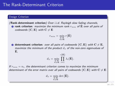
The Rank-Determinant Criterion
Design Criterion
(Rank-determinant criterion) Over i.i.d. Rayleigh slow fading channels,1 rank criterion: maximize the minimum rank rmin of E over all pairs ofcodewords C,E with C 6= E
rmin = minC,EC 6=E
r(E)
2 determinant criterion: over all pairs of codewords C,E with C 6= E,maximize the minimum of the product dλ of the non-zero eigenvalues ofE,
dλ = minC,EC 6=E
r(E)∏
i=1
λi
(E).
If rmin = nt, the determinant criterion comes to maximize the minimumdeterminant of the error matrix over all pairs of codewords C,E with C 6= E
dλ = minC,EC 6=E
det(E).
134 / 273

The Rank-Determinant Criterion
Definition
A full-rank (a.k.a. full-diversity) code is characterized by rmin = nt. Arank-deficient code is characterized by rmin < nt.
Example
Rank-deficient and full-rank codes for nt = 2• Rank-deficient code
C =1√2
[c1c2
]
,E =1√2
[e1e2
]
• Full-rank code
C =1√2
[c1 −c∗2c2 c∗1
]
,E =1√2
[e1 −e∗2e2 e∗1
]
(C−E) (C−E)H =1
2
[|c1 − e1|2 + |c2 − e2|2 0
0 |c1 − e1|2 + |c2 − e2|2]
135 / 273

The Rank-Determinant Criterion
Example
Question: Relying on the rank-determinant criterion, show that delay diversityachieves full diversity. Assume for simplicity two transmit antennas.Answer: The codeword for delay diversity can be written as
C =1√2
[c1 c2 . . . cT−1 00 c1 c2 . . . cT−1
]
.
Taking another codeword E, different from C,
E =1√2
[e1 e2 . . . eT−1 00 e1 e2 . . . eT−1
]
.
The diversity gain is given by the minimum rank of the error matrix over allpossible pairs of (different) codewords, i.e.
rmin = minC,EC 6=E
r(E)= min
C,EC 6=E
r(C−E
).
136 / 273

The Rank-Determinant Criterion
Example
With delay diversity, we have
C−E =1√2
[c1 − e1 c2 − e2 . . . cT−1 − eT−1 0
0 c1 − e1 c2 − e2 . . . cT−1 − eT−1
]
.
Obviously, r(C−E
)≤ 2. Actually, r
(C−E
)= 2 as long as C 6= E. Indeed
even in the case where all ck − ek = 0 except for one index k (in order to keepC 6= E), e.g. k = 1,
C−E =1√2
[c1 − e1 0 . . . 0 0
0 c1 − e1 0 . . . 0
]
,
the rank is equal to 2. Hence diversity gain of 2nr.
137 / 273

The Rank-Determinant Criterion
Example
Question: Assume that c1, c2, c3 and c4 are constellation symbols taken from aunit average energy QAM constellation. Consider the Linear Space-Time BlockCode, characterized by codewords
C =1
2
[c1 + c3 c2 + c4c2 − c4 c1 − c3
]
.
What is the diversity gain achieved by this code over slow Rayleigh fadingchannels?Answer: Check the rank of its error matrix
C−E =1
2
[d1 + d3 d2 + d4d2 − d4 d1 − d3
]
where dk = ck − ek for k = 1, ..., 4. This code is rank deficient. It is easily seenthat by taking two codewords C and E such that d3 = d4 = 0 andd1 = d2 = d (which is encountered for any constellations), r (C−E) = 1.Hence diversity gain of nr.
138 / 273

Information Theory Motivated Design Methodology: FastFading MIMO Channels - Achieving The Ergodic Capacity
• Recall Lecture on ergodic capacity
C = maxQ:TrQ=1
E
log2 det(
Inr + ρHQHH)
.
• Perfect Transmit Channel Knowledge– transmit independent streams in the directions of the eigenvectors of the channel
matrix H.– For a total transmission rate R, each stream k can then be encoded using a
capacity-achieving Gaussian code with rate Rk such that∑n
k=1Rk = R, ascribed apower λk (Q) and be decoded independently of the other streams.
– The optimal power allocationλ⋆kbased on the water-filling allocation strategy.
– Capacity achievable using a variable-rate coding strategy (T = Tcoh is enough as longas the noise can be averaged out).
• Partial Transmit Channel Knowledge– When the channel is i.i.d. Rayleigh fading, Q = (1/nt) Int .– Transmission of independent information symbols may be performed in parallel over n
virtual spatial channels.– The transmitter is very similar to the CSIT case except that all eigenmodes now receive
the same amount of power.– Transmit with uniform power allocation over nt independent streams, each stream
using an AWGN capacity-achieving code and perform joint ML decoding (independentdecoding of all streams is clearly suboptimal due to interference between streams).
139 / 273

Information Theory Motivated Design Methodology: SlowFading MIMO Channels Achieving The DMT
• Impossible to code over a large number of independent channel realizations →separate coding leads to an outage as soon as one of the subchannels is in deep fade.
• Joint coding across all subchannels necessary in the absence of transmit channelknowledge!
• Rank-determinant criterion focuses on diversity maximization under fixed rate.• What if we want to design codes achieving the diversity-multiplexing trade-off?
Definition
A schemeC(ρ)
, i.e., a family of codes indexed by the SNR ρ, is said toachieve a diversity gain gd (gs,∞) and a multiplexing gain gs at high SNR if
limρ→∞
R(ρ)
log2(ρ) = gs
limρ→∞
log2(Pe
(ρ))
log2(ρ) = −gd (gs,∞)
where R(ρ)is the data rate and Pe
(ρ)the average error probability averaged
over the additive noise, the i.i.d. channel statistics and the transmittedcodewords. The curve gd (gs,∞) is the diversity-multiplexing trade-off achievedby the scheme in the high SNR regime.
140 / 273

Space-Time Block Coding (STBC)
• STBCs can be seen as a mapping of Q symbols (complex or real) onto a codewordC of size nt × T .
• Codewords are uncoded in the sense that no error correcting code is contained in theSTBC.
• Linear STBCs are by far the most widely used– Spread information symbols in space and time in order to improve either the diversity
gain, either the spatial multiplexing rate (rs = QT) or both the diversity gain and the
spatial multiplexing rate.– Pack more symbols into a given codeword, i.e., increase Q, to increase the data rate.
Example
Alamouti code: nt = 2, Q = 2, T = 2, rs = 1
C =1√2
[c1 −c∗2c2 c∗1
]
.
141 / 273

A General Framework for Linear STBCs
• A linear STBC is expressed in its general form as
C =
Q∑
q=1
Φqℜ[cq ] +Φq+Qℑ[cq]
where– Φq are complex basis matrices of size nt × T ,– cq stands for the complex information symbol (taken for example from PSK or QAM
constellations),– Q is the number of complex symbols cq transmitted over a codeword,– ℜ and ℑ stand for the real and imaginary parts.
Definition
Tall (T ≤ nt) unitary basis matrices are such that ΦHq Φq = 1
QIT
∀q = 1, . . . , 2Q. Wide (T ≥ nt) unitary basis matrices are such thatΦqΦ
Hq = T
QntInt ∀q = 1, . . . , 2Q.
Definition
The spatial multiplexing rate of a space-time block code is defined as rs = QT.
A full rate space-time block code is characterized by rs = nt.
142 / 273

A General Framework for Linear STBCs
• Average Pairwise Error Probability of STBCs
Proposition
A PSK/QAM based linear STBC consisting of unitary basis matrices minimizesthe worst-case PEP averaged over i.i.d. Rayleigh slow fading channels if(sufficient condition) the unitary basis matrices Φq2Qq=1 satisfy the conditions
ΦqΦHp +ΦpΦ
Hq = 0nt , q 6= p for wide Φq2Qq=1,
ΦHq Φp +Φ
Hp Φq = 0T , q 6= p for tall Φq2Qq=1.
Proof: Using Hadamard’s inequality and the unitarity of basis matrices,
minq=1,...,Q
mindq
det(Int + ηE
)≤ det
(
Int + ηT
QntIntd
2min
)
.
Equality if unitary basis matrices are skew-hermitian.
143 / 273

A General Framework for Linear STBCs
• Decoding
Proposition
Applying the space-time matched filter to the output vector decouples thetransmitted symbols if and only if the basis matrices are wide unitary
ΦqΦHq =
T
QntInt , ∀q = 1, . . . , 2Q
and pairwise skew-hermitian
ΦqΦHp +ΦpΦ
Hq = 0nt , ∀q 6= p.
The complexity of ML decoding of linear STBCs grows exponentially with nt and Q.The decoupling property allows each symbol to be decoded independently of thepresence of the other symbols through a simple space-time matched filter.
144 / 273

A General Framework for Linear STBCs
Example
A code such that T = 1, nt = 2, Q = 2, rs = 2 with the following tall basismatrices
Φ1 =1√2
[10
]
, Φ2 =1√2
[01
]
, Φ3 =1√2
[j0
]
, Φ4 =1√2
[0j
]
,
This code is called Spatial Multiplexing. Optimal for worst-case PEP min.spectrally-efficient, large decoding complexity.
145 / 273
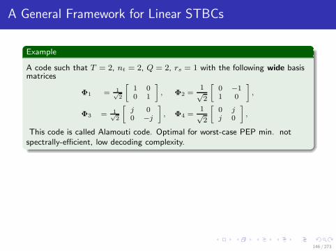
A General Framework for Linear STBCs
Example
A code such that T = 2, nt = 2, Q = 2, rs = 1 with the following wide basismatrices
Φ1 = 1√2
[1 00 1
]
, Φ2 =1√2
[0 −11 0
]
,
Φ3 = 1√2
[j 00 −j
]
, Φ4 =1√2
[0 jj 0
]
,
This code is called Alamouti code. Optimal for worst-case PEP min. notspectrally-efficient, low decoding complexity.
146 / 273

Spatial Multiplexing/V-BLAST/D-BLAST
• Spatial Multiplexing (SM), also called V-BLAST, is a full rate code (rs = nt) thatconsists in transmitting independent data streams on each transmit antenna.
• In uncoded transmissions, we assume one symbol duration (T = 1) and codeword C
is a symbol vector of size nt × 1.
Example
C =1√nt
[c1 . . . cnt
]T=
1√nt
nt∑
q=1
Int (:, q)ℜ [cq ] + jInt (:, q)ℑ [cq] .
Each element cq is a symbol chosen from a given constellation.
147 / 273

ML decoding
• Error probability
P (C→ E) =1
π
∫ π/2
0
[
det(
Int + ηE)]−nr
dβ
=1
π
∫ π/2
0
(
1 +η
nt
nt∑
q=1
|cq − eq|2)−nr
dβ
≤(
ρ
4nt
)−nr
(nt∑
q=1
|cq − eq|2)−nr
The SNR exponent is equal to nr. Due to the lack of coding across transmitantennas, no transmit diversity is achieved and only receive diversity is exploited.
• Over fast fading channels, we know that it is not necessary to code across antennasto achieve the ergodic capacity.
Proposition
Spatial Multiplexing with ML decoding and equal power allocation achieves theergodic capacity of i.i.d. Rayleigh fast fading channels.
148 / 273

ML decoding
• Over slow fading channels, what is the multiplexing-diversity trade-off achieved bySM with ML decoding?
Proposition
For nr ≥ nt, the diversity-multiplexing trade-off at high SNR achieved bySpatial Multiplexing with ML decoding and QAM constellation over i.i.d.Rayleigh fading channels is given by
gd (gs,∞) = nr
(
1− gsnt
)
, gs ∈ [0, nt] .
149 / 273

Zero-Forcing (ZF) Linear Receiver
• MIMO ZF receiver acts similarly to a ZF equalizer in frequency selective channels.
• ZF filtering effectively decouples the channel into nt parallel channels– interference from other transmitted symbols is suppressed– scalar decoding may be performed on each of these channels
• The complexity of ZF decoding similar to SISO ML decoding, but the inversion stepis responsible for the noise enhancement (especially at low SNR).
• Assuming that a symbol vector C = 1/√nt
[c1 . . . cnt
]Tis transmitted, the
output of the ZF filter GZF is given by
z = GZFy =[c1 . . . cnt
]T+GZFn
where GZF inverts the channel,
GZF =
√nt
EsH
†
with H† =(HHH
)−1HH denoting the Moore-Penrose pseudo inverse.
150 / 273

Zero-Forcing (ZF) Linear Receiver
• Covariance matrix of the noise at the output of the ZF filter
E
GZFn (GZFn)H
=nt
ρH
†(
H†)H
=nt
ρ
(
HHH)−1
.
• The output SNR on the qth subchannel is thus given by
ρq =ρ
nt
1
(HHH)−1 (q, q), q = 1, . . . , nt.
• Inversion leads to noise enhancement. Severe degradation at low SNR.• Assuming that the channel is i.i.d. Rayleigh distributed, ρq is a χ2 random variable
with 2 (nr − nt + 1) degrees of freedom, denoted as χ22(nr−nt+1). The average PEP
on the qth subchannel is thus upper-bounded by
P (cq → eq) ≤(
ρ
4nt
)−(nr−nt+1)
|cq − eq|−2(nr−nt+1) .
The lower complexity of the ZF receiver comes at the price of a diversity gain limitedto nr − nt + 1. Clearly, the system is undetermined if nt > nr.
151 / 273

Zero-Forcing (ZF) Linear Receiver
• In fast fading channels, the average maximum achievable rate CZF is equal to thesum of the maximum rates achievable by all layers
CZF =
minnt,nr∑
q=1
E log2 (1 + ρq)
(ρր)≈ min nt, nr log2
(ρ
nt
)
+min nt, nr Elog2
(χ22(nr−nt+1)
).
Note the difference with
CCDIT ≈ nlog2
( ρ
nt
)
+n∑
k=1
E
log2(χ22(N−n+k))
.
Spatial Multiplexing in combination with a ZF decoder allows for transmitting overn = min nt, nr independent data pipes.
152 / 273

Zero-Forcing (ZF) Linear Receiver
• In slow fading channels, what is the diversity-multiplexing trade-off achieved by SMwith ZF?
Proposition
For nr ≥ nt, the diversity-multiplexing trade-off achieved by SpatialMultiplexing with QAM constellation and ZF filtering in i.i.d. Rayleigh fadingchannels is given by
gd (gs,∞) = (nr − nt + 1)
(
1− gsnt
)
, gs ∈ [0, nt] .
153 / 273

Zero-Forcing (ZF) Linear Receiver
• ZF receiver maximizes the SNR under the constraint that the interferences from allother layers are nulled out.
– For a given layer q, the ZF combiner gq is such that this layer is detected through aprojection of the output vector y onto the direction closest to H (:, q) within thesubspace orthogonal to the one spanned by the set of vectors H (:, p), p 6= q.
• Assume the following system model with nr ≥ nt
y = Hc+ n,
= hqcq +∑
p 6=q
hpcp + n
where hq is the qth column of H.• Let us build the following nr × (nt − 1) matrix by collecting all hp with p 6= q:
H−q =[. . . hp . . .
]
p 6=q,
=[U′ U
]ΛV
H
where U is the matrix containing the left singular vectors corresponding to the nullsingular values. Similarly we define
c−q =[. . . cp . . .
]T
p 6=q.
154 / 273

Zero-Forcing (ZF) Linear Receiver
• By multiplying by UH , we project the output vector onto the subspace orthogonal tothe one spanned by the columns of H−q
UHy = U
Hhqcq + U
HH−qc−q + U
Hn
= UHhqcq + U
Hn.
• To maximize the SNR, noting the noise is still white, we match to the effectivechannel UHhq such that
z =(
UHhq
)H
UHhqcq +
(
UHhq
)H
UHn
and the ZF combiner is gq =(
UHhq
)H
UH = hHq UUH .
155 / 273

Minimum Mean Squared Error (MMSE) Linear Receiver
• Filter maximizing the SINR. Minimize the total resulting noise: find G such that
E∥∥Gy −
[c1 . . . cnt
]T ∥∥2is minimum.
• The combined noise plus interference signal ni,q when estimating symbol cq writes as
ni,q =∑
p 6=q
√
Es
nthpcp + n.
The covariance matrix of ni,q reads as
Rni,q = E
ni,qnHi,q
= σ2nInr +
∑
p 6=q
Es
nthph
Hp
and the MMSE combiner for stream q is given by
gMMSE,q =
√
Es
nthHq
σ2nInr +
∑
p 6=q
Es
nthph
Hp
−1
.
• An alternative and popular representation of the MMSE filter can also be written as
GMMSE =
√nt
Es
(
HHH+
nt
ρInt
)−1
HH =
√nt
EsH
H
(
HHH +
nt
ρInr
)−1
• Bridge between matched filtering at low SNR and ZF at high SNR.156 / 273

Minimum Mean Squared Error (MMSE) Linear Receiver
• The output SINR on the qth subchannel (stream) is given by
ρq =Es
nthHq
σ2nInr +
∑
p 6=q
Es
nthph
Hp
−1
hq .
• At high SNR, the MMSE filter is practically equivalent to ZF and the diversityachievable is thus limited to nr − nt + 1.
157 / 273

Successive Interference Canceler
• Successively decode one symbol (or more generally one layer/stream) and cancel theeffect of this symbol from the received signal.
• Decoding order based on the SINR of each symbol/layer: the symbol/layer with thehighest SINR is decoded first at each iteration.
• SM with (ordered) SIC is generally known as V-BLAST, and ZF and MMSEV-BLAST refer to SM with respectively ZF-SIC and MMSE-SIC receivers.
• The diversity order experienced by the decoded layer is increased by one at eachiteration. Therefore, the symbol/layer detected at iteration i will achieve a diversityof nr − nt + i.
• Major issue: error propagation– The error performance is mostly dominated by the weakest stream.– Non-ordered SIC: diversity order approximately nr − nt + 1.– Ordered SIC: performance improved by reducing the error propagation caused by the
first decoded stream. The diversity order remains lower than nr .
158 / 273

Successive Interference Canceler
1 Initialization: i←− 1, y(1) = y,G(1) = GZF (H),q1(∗)= argminj
∥∥G(1) (j, :)
∥∥2
where GZF (H) is defined as the ZF filter of the matrix H.2 Recursion:
1 step 1: extract the qthi transmitted symbol from the received signal y(i)
cqi = G(i) (qi, :)y(i)
where G(i) (qi, :) is the qthi row of G(i);2 step 2: slice cqi to obtain the estimated transmitted symbol cqi ;3 step 3: assume that cqi = cqi and construct the received signal
y(i+1) = y(i) −√
Es
ntH (:, qi) cqi
G(i+1) = GZF
(Hqi
)
i ←− i+ 1
qi+1(∗)= arg min
j /∈q1,...,qi
∥∥G(i+1) (j, :)
∥∥2
where Hqi is the matrix obtained by zeroing columns q1, . . . , qi of H. Here
GZF
(Hqi
)denotes the ZF filter applied to Hqi .
159 / 273

Successive Interference Canceler
• In fast fading channels, the maximum rate achievable with ZF-SIC
CZF−SIC =
minnt,nr∑
q=1
E log2 (1 + ρq)
(ρր)≈ min nt, nr log2
(ρ
nt
)
+
minnt,nr∑
q=1
Elog2
(χ22(nr−nt+q)
)= CCDIT
The loss that was observed with ZF filtering is now compensated because thesuccessive interference cancellation improves the SNR of each decoded layer.
Proposition
Spatial Multiplexing with ZF-SIC (ZF V-BLAST) and equal power allocationachieves the ergodic capacity of i.i.d. Rayleigh fast fading MIMO channels atasymptotically high SNR.
This only holds true when error propagation is neglected.
160 / 273

Successive Interference Canceler
• MMSE-SIC does better for any SNR
CMMSE−SIC =
minnt,nr∑
q=1
E log2 (1 + ρq) = E
log2 det
(
Inr +ρ
ntHH
H
)
= Ie,
Proposition
Spatial Multiplexing with MMSE-SIC (MMSE V-BLAST) and equal powerallocation achieves the ergodic capacity for all SNR in i.i.d. Rayleigh fast fadingMIMO channels.
Result also valid for a deterministic channel.
161 / 273

Successive Interference Canceler
• In slow fading channels, what is the diversity-multiplexing trade-off achieved byunordered ZF-SIC?
Proposition
For nr ≥ nt, the diversity-multiplexing trade-off achieved by SpatialMultiplexing with QAM constellation and unordered ZF-SIC receiver over i.i.d.Rayleigh fading channels is given by
gd (gs,∞) = (nr − nt + 1)
(
1− gsnt
)
, gs ∈ [0, nt] .
The achieved trade-off is similar to the trade-off achieved by a simple ZF receiver.This comes from the fact that the first layer dominates the error probability since itserror exponent is the smallest.
• By increasing the number of receive antennas by 1,– with ZF or unordered ZF-SIC, we can either accommodate one extra stream with the
same diversity order or increase the diversity order of every stream by 1,– with ML, we can accommodate one extra stream and simultaneously increase the
diversity order of every stream by 1.
162 / 273

Impact of Decoding Strategy on Error Probability
• SM with ML, ordered and non ordered ZF SIC and simple ZF decoding in 2× 2 i.i.d.Rayleigh fading channels for 4 bits/s/Hz.
0 5 10 15 20 2510
−4
10−3
10−2
10−1
100
SNR [dB]
BER
MLordered ZF SICZF SICZF
The slope of the ML curve approaches 2. ZF only achieves a diversity order ofnr − nt + 1 = 1.
163 / 273

Impact of Decoding Strategy on Error Probability
• SM with ML, ZF and MMSE in i.i.d. Rayleigh slow fading channels withnt = nr = 4 and QPSK.
0 5 10 15 20 2510
−4
10−3
10−2
10−1
100
SNR [dB]
BE
R
MLMMSEZF
164 / 273

Orthogonal Space-Time Block Codes
• O-STBC vs. SM– Remarkable properties which make them extremely easy to decode: MIMO ML
decoding decouples into several SIMO ML decoding– Achieve a full-diversity of ntnr.– Much smaller spatial multiplexing rate than SM.
• Linear STBC characterized by the two following properties1 the basis matrices are wide unitary
ΦqΦHq =
T
QntInt ∀q = 1 . . . 2Q
2 the basis matrices are pairwise skew-hermitian
ΦqΦHp +ΦpΦ
Hq = 0, q 6= p
or equivalently by this unique property
CCH =
T
Qnt
[Q∑
q=1
|cq |2]
Int .
• Complex O-STBCs with rs = 1 only exist for nt = 2. For larger nt, codes exist withrs ≤ 1/2. For some particular values of nt > 2, complex O-STBCs with1/2 < rs < 1 have been developed. This is the case for nt = 3 and nt = 4 withrs = 3/4.
165 / 273

Orthogonal Space-Time Block Codes
Example
Alamouti code: complex O-STBC for nt = 2 with a spatial multiplexing raters = 1
C =1√2
[c1 −c∗2c2 c∗1
]
.
• basis matrices are unitary and skew-hermitian (discussed before).
• CCH = 12
[|c1|2 + |c2|2
]I2.
• rs = 1 since two symbols are transmitted over two symbol durations.
Example
For nt = 3 , a complex O-STBC expanding on four symbol durations (T = 4)and transmitting three symbols on each block (Q = 3)
C =2
3
c1 −c∗2 c∗3 0c2 c∗1 0 c∗3c3 0 −c∗1 −c∗2
.
The spatial multiplexing rate rs is equal to 3/4.166 / 273

Orthogonal Space-Time Block Codes
Proposition
O-STBCs enjoy the decoupling property.
Example
Assume a MISO transmission based on the Alamouti code
[y1 y2
]=
√
Es
2
[h1 h2
][
c1 −c∗2c2 c∗1
]
+[n1 n2
]
or equivalently
[y1y∗2
]
=
√
Es
2
[h1 h2
h∗2 −h∗
1
]
︸ ︷︷ ︸
Heff
[c1c2
]
+
[n1
n∗2
]
.
167 / 273

Orthogonal Space-Time Block Codes
Example
Applying the space-time matched filter HHeff to the received vector decouples
the transmitted symbols
[z1z2
]
= HHeff
[y1y∗2
]
=
√
Es
2
[|h1|2 + |h2|2
]I2
[c1c2
]
+HHeff
[n1
n∗2
]
.
Expanding the original ML metric
∣∣∣∣y1 −
√
Es
2(h1c1 + h2c2)
∣∣∣∣
2
+
∣∣∣∣y2 −
√
Es
2(−h1c
∗2 + h2c
∗1)
∣∣∣∣
2
and making use of z1 and z2, the decision metric for c1 is
choose ci iff
∣∣∣∣z1−
√
Es
2
(|h1|2 + |h2|2
)ci
∣∣∣∣
2
≤∣∣∣∣z1−
√
Es
2
(|h1|2 + |h2|2
)ck
∣∣∣∣
2
∀i 6= k
and similarly for c2. Independent decoding of symbols c1 and c2 is soperformed.
168 / 273

Orthogonal Space-Time Block Codes
• Error Probability
P (C→ E) =1
π
∫ π/2
0
[
det(
Int + ηE)]−nr
dβ
=1
π
∫ π/2
0
(
1 + ηT
Qnt
Q∑
q=1
|cq − eq|2)−nrnt
dβ
(ρր)
≤(ρ
4
T
Qnt
)−nrnt
(Q∑
q=1
|cq − eq|2)−nrnt
.
Full diversity gain of ntnr.
169 / 273

Orthogonal Space-Time Block Codes
• O-STBCs are not capacity efficient IO−STBC (H) ≤ Ie (H)– mutual information of MIMO channel
Ie (H) = log2
(
1 +ρ
nt‖H‖2F + . . .+
(ρ
nt
)r(H) r(H)∏
k=1
λk
(
HHH))
.
– mutual information of MIMO channel transformed by the O-STBC
IO−STBC (H) =Q
Tlog2
(
1 +ρT
Qnt‖H‖2F
)
.
Proposition
For a given channel realization H, the mutual information achieved by anyO-STBC is always upper-bounded by the channel mutual information withequal power allocation Ie. Equality occurs if and only if both the rank of thechannel and the spatial multiplexing rate of the code are equal to one.
Corollary
The Alamouti scheme is optimal with respect to the mutual information whenused with only one receive antenna.
170 / 273

Orthogonal Space-Time Block Codes
• Diversity-Multiplexing Trade-off Achieved by O-STBCs
Proposition
The diversity-multiplexing trade-off at high SNR achieved by O-STBCs usingQAM constellations in i.i.d. Rayleigh fading channels is given by
gd (gs,∞) = nrnt
(
1− gsrs
)
, gs ∈ [0, rs] .
Proposition
The Alamouti code with any QAM constellation achieves the optimaldiversity-multiplexing trade-off for two transmit and one receive antennas ini.i.d. Rayleigh fading channels.
171 / 273

Orthogonal Space-Time Block Codes
• Block error rate for 4 different rates R = 4, 8, 12, 16 bits/s/Hz in 2× 2 i.i.d. slowRayleigh fading channels.
0 10 20 30 40 50 60
10−5
10−4
10−3
10−2
10−1
100
SNR [dB]
(2x2
) B
lock E
rro
r R
ate
<−−−12dB−−−>M=4, R=4
M=16, R=8
M=64, R=12
M=256, R=16
– full diversity exploited: gd (gs = 0,∞) = god (∞) = 4.– the growth of the multiplexing gain is slow: 12 dB separate the curves, corresponding
to a multiplexing gain gs = 1, i.e., 1 bit/s/Hz increase per 3 dB SNR increase.172 / 273

Other Code Constructions
• Quasi-Orthogonal Space-Time Block Codes– increase the spatial multiplexing rate while still partially enjoying the decoupling
properties of O-STBCs– use O-STBCs of reduced dimensions as the building blocks of a higher dimensional code
• Linear Dispersion Codes– if a larger receiver complexity is authorized, it is possible to relax the skew-hermitian
conditions and increase the data rates while still providing transmit diversity.
• Algebraic Space-Time Codes– structured codes using algebraic tools– many of them are designed to achieve the optimal diversity-multiplexing tradeoff
173 / 273
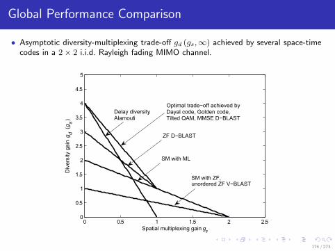
Global Performance Comparison
• Asymptotic diversity-multiplexing trade-off gd (gs,∞) achieved by several space-timecodes in a 2× 2 i.i.d. Rayleigh fading MIMO channel.
0 0.5 1 1.5 2 2.50
0.5
1
1.5
2
2.5
3
3.5
4
4.5
5
Spatial multiplexing gain gs
Div
ers
ity g
ain
gd
(gs
)
SM with ZF,unordered ZF V−BLAST
SM with ML
Delay diversity,Alamouti
ZF D−BLAST
Optimal trade−off achieved byDayal code, Golden code,Tilted QAM, MMSE D−BLAST
174 / 273

Global Performance Comparison
• Bit error rate (BER) of several space-time block codes in i.i.d. slow Rayleigh fadingchannels with nt = 2 and nr = 2 in a 4-bit/s/Hz transmission. ML decoding is used.
10 12 14 16 18 2010
−4
10−3
10−2
10−1
SNR [dB]
BER
SMAlamoutiDayalTASTB2,φ
Tilted−QAM
175 / 273

Example
Question: Here is the average Error Probability of one scheme (i.e., onetransmission and reception strategy) vs. SNR for point-to-point channels withi.i.d. Rayleigh slow fading and four different antenna configurations (a) to (d).The CSI is unknown to the transmitter.
0 10 20 30 40 50 6010
−8
10−7
10−6
10−5
10−4
10−3
10−2
10−1
100
SNR [dB]
Err
or P
roba
bilit
y
(a)(b)(c)(d)
176 / 273

Example
Question: What is the diversity gain (at high SNR) achieved by that scheme ineach antenna configuration? Provide your reasoning.
Answer: The diversity gain is the slope at high SNR of the error curve vs. theSNR on a log-log scale, i.e. − limρ→∞
log(Pe(ρ))log(ρ)
with ρ being the SNR.
For (a), the diversity gain is 1 as the error rate decreases by 10−1 when theSNR is increased from 50dB to 60dB.For (b), the diversity gain is 2 as the error rate decreases by 10−2 when theSNR is increased from 30dB to 40dB.For (c), the diversity gain is 3 as the error rate decreases by 10−3 when theSNR is increased from roughly 26dB to 36dB.For (d), the diversity gain is 4 as the error rate decreases by 10−4 when theSNR is increased from 10dB to 20dB.
177 / 273

Example
Question: For each scenario (a) to (d), identify an antenna configuration (i.e.,nt and nr) and the corresponding transmission/reception strategy that canachieve such diversity gain. Provide your reasoning.
Answer: The simplest approach is to performfor (a), receive matched filter with nr = 1, nt = 1for (b), receive matched filter with nr = 2, nt = 1for (c), receive matched filter with nr = 3, nt = 1for (d), receive matched filter with nr = 4, nt = 1
Alternative strategies are possible, for instance selection combining at thereceiver for all 4 cases. We could also perform transmit diversity based onspace-time coding and use O-STBC for (b),(c),(d) to achieve diversity order of2 with nt = 2 and nr = 1, 3 with nt = 3 and nr = 1, 4 with nt = 4 andnr = 1, respectively. Alternatively, we could as well use Spatial Multiplexingwith ZF receiver and transmit two streams over two transmit antennas and use2,3,4,5 receive antennas for a,b,c,d respectively.
178 / 273

MIMO with Partial Channel State Information at
the Transmitter
179 / 273

Reference Book
• Bruno Clerckx and Claude Oestges, “MIMO Wireless Networks: Channels,Techniques and Standards for Multi-Antenna, Multi-User and Multi-Cell Systems,”Academic Press (Elsevier), Oxford, UK, Jan 2013.
– Chapter 10
Section: 10.1, 10.2.1, 10.5, 10.6.1,10.6.2, 10.6.3, 10.6.4, 10.9
180 / 273

Introduction
• full CSIT– array and diversity gain– lower system complexity (parallel virtual transmissions)– hardly achievable (especially when the channel varies rapidly), costly in terms of
feedback
• Exploiting Channel Statistics at the Transmitter– low rate feedback link– statistical properties of the channel (correlations, K-factor) vary at a much slower rate
than the fading channel itself– The receiver estimates the channel stochastic properties and sends them back to the
transmitter “once in a while” (if channel reciprocity cannot be exploited)– stationary channel: statistics do not change over time
• Exploiting a Limited Amount of Feedback at the Transmitter– codebook of precoding matrices, i.e., a finite set of precoders, designed off-line and
known to both the transmitter and receiver.– The receiver estimates the best precoder as a function of the current channel and feeds
back only the index of this best precoder in the codebook.
181 / 273

System Model
• MIMO system with nt transmit and nr receive antennas communicating through afrequency flat slow fading channel.
• The encoder outputs a codeword C = [c0 . . . cT−1] of size ne × T contained in thecodebook C over T symbol durations.
• Precoder P [nt × ne] processes the codeword C and the codeword C′ = PC
[nt × T ] is transmitted over nt antennas.
S
constellation shaper
W
beamformer
P
C’’C C’1/2
• Linear precoder P = WS1/2
– multi-mode beamformer W whose columns have a unit-norm– constellation shaper S1/2 (if S real-valued and diagonal, it can be thought of as the
power allocation scheme across the modes)
• nomalization: ETrC′C′H = T , E
TrCCH
= T and Tr
PPH
= ne,
E‖H‖2F
= ntnr.
182 / 273

Channel Statistics based Precoding
• Information Theory motivated strategy.
Proposition
In Kronecker correlated Rayleigh fast fading channels, the optimal inputcovariance matrix can again be expressed as
Q = URtΛQUHRt
,
where URt is a unitary matrix formed by the eigenvectors of Rt (arranged insuch order that they correspond to decreasing eigenvalues of Rt), and ΛQ is adiagonal matrix whose elements are also arranged in decreasing order.
Transmit a single stream along the dominant eigenvector of Rt if very large transmitcorrelation. Transmit multiple streams with uniform power allocation if very lowtransmit correltion.
• Error Probability motivated strategy
P⋆ = argmin
PmaxE 6=0
P (C→ E)
– challenging problem for arbitrary codes– focus on O-STBC
183 / 273
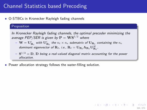
Channel Statistics based Precoding
• O-STBCs in Kronecker Rayleigh fading channels
Proposition
In Kronecker Rayleigh fading channels, the optimal precoder minimizing theaverage PEP/SER is given by P = WS1/2 where
– W = U′Rt
with U′Rt
the nt × ne submatrix of URt containing the ne
dominant eigenvector of Rt, i.e., Rt = URtΛRtUHRt
,
– S1/2 = D, D being a real-valued diagonal matrix accounting for the powerallocation.
• Power allocation strategy follows the water-filling solution.
184 / 273

Channel Statistics based Precoding
Example
Let us consider the Alamouti O-STBC with two transmit antennas(ne = nt = 2). Denoting S = diag s1, s2, the transmitted codewords areproportional, at the first time instant, to
1√2URtS
1/2
[c1c2
]
=1√2URt (:, 1)
√s1c1 +
1√2URt (:, 2)
√s2c2
and, at the second time instant, to
1√2URtS
1/2
[−c∗2c∗1
]
= − 1√2URt (:, 1)
√s1c
∗2 +
1√2URt (:, 2)
√s2c
∗1.
Extreme cases:• s1 = s2 = 1: Alamouti scheme
• s1 = 2, s2 = 0: beamforming in the dominant eigenbeamThe precoder allocates more power to angular directions corresponding to thepeaks of the transmit direction power spectrum.
185 / 273

Channel Statistics based Precoding
• Performance of a transmit correlation based precoded Alamouti scheme in 2× 2transmit correlated (t = 0.7 and t = 0.95) Rayleigh channels
0 2 4 6 8 10 1210
−3
10−2
10−1
SNR [dB]
BER
t = 0 .7, Alamoutit = 0 .7, Alamouti with precodert = 0 .7, single mode eigenbeamformingt = 0 .7, dominant eigenmode transmissioni.i.d., Alamouti
0 2 4 6 8 10 12 1410
−3
10−2
10−1
SNR [dB]BER
t = 0 .95, Alamoutit = 0 .95, Alamouti with precodert = 0 .95, dominant eigenmode transmissioni.i.d., Alamouti
186 / 273

Quantized Precoding: dominant eigenmode transmission
• Assume dominant eigenmode transmission (i.e. beamforming)
y =√EsHwc+ n,
z = gHy,
=√Esg
HHwc+ g
Hn
where g and w are respectively nr × 1 and nt × 1 vectors.• Assuming MRC, the optimal beamforming vector w that maximizes the SNR is given
byw
⋆ = arg maxw∈Cw
‖Hw‖2
with Cw set of unit-norm vectors. The best precoder is the dominant right singularvector of H.
• Reduce the number of feedback bits: limit the space Cw over which w can be chosento a codebook called W. The receiver evaluates the best precoder w⋆ among allunit-norm precoders wi ∈ W (with i = 1, . . . , np) such that
w⋆ = arg max
1≤i≤npwi∈W
‖Hwi‖2 .
187 / 273

Quantized Precoding: distortion function
• How to design the codebook? Need for a distortion function, i.e. measure of theaverage (over all channel realizations) array gain loss induced by the quantizationprocess
df = EH
λmax − ‖Hw⋆‖2
• Upper-bound
df ≤ EH
λmax − λmax
∣∣∣v
Hmaxw
⋆∣∣∣
2
,
(a)= EH λmax
︸ ︷︷ ︸
quality of the channel
EH
1−∣∣∣v
Hmaxw
⋆∣∣∣
2
︸ ︷︷ ︸
quality of the codebook
where vmax is the dominant right singular vector of H. Equality (a) is only valid fori.i.d. Rayleigh fading channels.
188 / 273

Quantized Precoding: Lloyd
• Generalized Lloyd Algorithm:
Algorithm
For the given codebook, find the optimal quantization cells using the nearestneighbor rule. For the so-obtained quantization cells, determine that optimalquantized precoders using the centroid condition. Iterate till convergence.
• Essential conditions:– Assume MISO channel.– centroid condition: the optimal quantized precoder wk of any quantization cell Rk is
to be chosen as the dominant eigenvector of Rk = EhHh |h ∈ Rk
.
– nearest neighbor rule: all channel vectors that are closer to the quantized precoder wkare assigned to quantization cell Rk, i.e. h ∈ Rk if ‖h‖2 − |hwk|2 ≤ ‖h‖2 − |hwj |2,
• Optimal codebook design for arbitrary fading channels
189 / 273

Quantized Precoding: Grassmannian
• Grassmannian Line Packing
Design Criterion
Choose a codebook W made of np unit-norm vectors wi (i = 1, . . . , np) suchthat the minimum distance
δline (W) = min1≤k<l≤np
√
1− |wHk wl|2,
is maximized.
– Problem of packing np lines in Cnt insuch a way that the minimum distancebetween any pair of lines is maximized.
– Close to optimal only for i.i.d. RayleighFading Channels.
190 / 273

Quantized Precoding: How many bits?
• How many feedback bits B = log2 (np) are required? In i.i.d. channels
Cquant ≈ Eh
log2
(
1 + ρ ‖h‖2(
1− 2− B
nt−1
))
,
leading to an SNR degradation of 10 log10
(
1− 2− B
nt−1
)
dB relative to perfect
CSIT.
Proposition
In order to maintain a constant SNR or capacity gap between perfect CSIT andquantized feedback, it is not necessary to scale the number of feedback bits asa function of the SNR. The multiplexing gain gs is not affected by the qualityof CSIT.
• Achievable diversity gain?– Antenna selection (AS) is a particular case of a quantized precoding whose codebook is
chosen as the columns of the identity matrix Int .– AS achieves a diversity gain of nt.– Sufficient to take a full rank codebook matrix with np ≥ nt to extract the full diversity
191 / 273

Quantized Precoding: Evaluations
• SER of a 3× 3 MIMO system using 2-bit and 6-bit quantized BPSK-based DET.
0 1 2 3 4 5 6
10−4
10−3
10−2
SNR [dB]
SER
2-bit D-DET6-bit Q-DETant. selectionP-DET
Example
Codebook for quantized DET fornt = 3 and np = 4.
W =
1√3
1√3
1√3
,
j√3
−1√3
−j√3
,
−1√3
1√3
−1√3
,
−j√3
−1√3j√3
192 / 273

Example
Question: Discuss the validity of the following statement and detail yourargument: ’Consider a point-to-point i.i.d. MISO Rayleigh slow fading channelwith 4 transmit antennas and 1 receive antenna and a transmission strategybased on partial transmit channel knowledge consisting of transmitting a singlestream using quantized precoding. The codebook of precoders is given by
W =
1000
,
0100
,
0010
.
This transmission strategy achieves a diversity gain of 4.’
193 / 273

Example
Answers: The codebook only contains 3 precoders. Looking at the precoder,no stream can be transmitted on the fourth antenna. The fourth antenna istherefore useless. This implies that the system effectively looks like a MISOwith 3 transmit antenna where transmit antenna selection is performed. Withnr antennas, receive antenna selection achieves a diversity gain of nr (seelecture notes). Similarly, transmit antenna selection achieves a diversity equalto 3 in this scenario. Hence the proposed strategy will achieve a diversity gainof 3. Hence the statement is wrong.
194 / 273

Quantized Precoding: spatially correlated channels
• Grassmiannian only appropriate for i.i.d. Rayleigh fading.• Spatial correlation decreases the quantization space compared to i.i.d. channels.
– e.g. Lloyd, adaptive/CDIT-based codebook, DFT (for uniform linear arrays)
• Normalized average distortion (SNR loss) df,n = df/EH λmax as a function of thecodebook size np = 2B and the transmit correlation coefficient t with nt = 4.
0 0.1 0.2 0.3 0.4 0.5 0.6 0.7 0.8 0.9 10
0.05
0.1
0.15
0.2
0.25
0.3
0.35
0.4
Magnitude of the transmit correlation coefficient t
Ave
rage
dis
tort
ion
d f,n
CDIT−based CB, B=3CDIT−based CB, B=4CDIT−based CB, B=5|t|−based CB, B=4DFT CB, B=4GLP CB, B=4
Wc =
R1/2t w1
∥∥R
1/2t w1
∥∥, . . . ,
R1/2t wnp
∥∥R
1/2t wnp
∥∥
195 / 273

Quantized Precoding: some extensions
• Extension to other kinds of channel models (e.g. spatial/time correlation,polarization), transmission strategies (e.g. O-STBCs, SM), reception strategies (e.g.MRC, ZF, MMSE, ML), criteria (e.g. error rate or transmission rate)
• Quantized precoding for SM with rank adaptation and rate maximization
W⋆ = argmax
ne
maxW
(ne)i
∈Wne
R.
The codebooks Wne are defined for ranks ne = 1, . . . ,min nt, nr. Rate is
computed on the equivalent precoded channel HW(ne)i .
– Uniform power allocation and joint ML decoding
R = log2 det
[
Ine +ρ
ne
(
W(ne)i
)HHHHW
(ne)i
]
.
– With other types of receivers/combiner
R =
ne∑
q=1
log2
(
1 + ρq(
HW(ne)i
))
.
where ρq is the SINR of stream q on at the output of the combiner for the equivalent
channel HW(ne)i .
196 / 273

Multi-User MIMO - Multiple Access Channels
(Uplink) & Broadcast Channels (Downlink)
197 / 273

Reference Book
• Bruno Clerckx and Claude Oestges, “MIMO Wireless Networks: Channels,Techniques and Standards for Multi-Antenna, Multi-User and Multi-Cell Systems,”Academic Press (Elsevier), Oxford, UK, Jan 2013.
– Chapter 12
Section: 12.1, 12.2, 12.3, 12.4
198 / 273

Introduction
• So far, we looked at a single link/user. Most systems are multi-user!• How to deal with multiple users? What is the benefit of MIMO in a multi-user
setting?• MIMO Broadcast Channel (BC) and Multiple Access Channel(MAC)
Differences between BC and MAC:– there are multiple independent receivers (and therefore multiple independent additive
noises) in BC while there is a single receiver (and therefore a single noise term) in MAC.– there is a single transmitter (and therefore a single transmit power constraint) in BC
while there are multiple transmitters (and therefore multiple transmit powerconstraints) in MAC.
– the desired signal and the interference (originating from the co-scheduled signals)propagate through the same channel in the BC while they propagate through differentchannels in the MAC.
199 / 273

MIMO MAC System Model
• Uplink multi-user MIMO (MU-MIMO) transmission– total number of K users (K = 1, . . . ,K) distributed in a cell,– nt,q transmit antennas at mobile terminal q (we simply drop the index q and write nt ifnt,q = nt ∀q)
– nr receive antenna at the base station
• Received signal (we drop the time dimension)
yul =
K∑
q=1
Λ−1/2q Hul,qc
′ul,q + nul
where– yul ∈ Cnr
– Hul,q ∈ Cnr×nt,q models the small scale time-varying fading process and Λ−1q refers
to the large-scale fading accounting for path loss and shadowing– nul is a complex Gaussian noise CN
(0, σ2nInr
).
• User q’s input covariance matrix is defined as the covariance matrix of the transmitsignal of user q as Qul,q = E
c′ul,qc
′ul,q
H.
• Power constraint: TrQul,q ≤ Es,q.
200 / 273

MIMO MAC System Model
• By stacking up the transmit signal vectors and the channel matrices of all K users,
c′ul =
[
c′Tul,1, . . . , c
′Tul,K
]T
,
Hul =[
Λ−1/21 Hul,1, . . . ,Λ
−1/2K Hul,K
]
,
the system model also writes as
yul = Hulc′ul + nul.
Hul is assumed to be full-rank as it would be the case in a typical user deployment.
• Long term SNR of user q defined as ηq = Es,qΛ−1q /σ2
n.
• Note on the notations: the dependence on the path loss and shadowing is madeexplicit in order to stress that the co-scheduled users experience different path lossesand shadowings and therefore receive power.
• We assume that the receiver (i.e. the BS in a UL scenario) has always perfectknowledge of the CSI, but we will consider strategies where the transmitters haveperfect or partial knowledge of the CSI.
201 / 273

Capacity Region of Deterministic Channels
• In a multi-user setup, given that all users share the same spectrum, the rateachievable by a given user q, denoted as Rq, will depend on the rate of the otherusers Rp, p 6= q → Trade-off between rates achievable by different users!
• The capacity region C formulates this trade-off by expressing the set of all user rates(R1, . . . , RK) that are simultaneously achievable.
Definition
The capacity region C of a channel Hul is the set of all rate vectors(R1, . . . , RK) such that simultaneously user 1 to user K can reliablycommunicate at rate R1 to rate RK , respectively.
Any rate vector not in the capacity region is not achievable (i.e. transmission atthose rates will lead to errors).
Definition
The sum-rate capacity C of a capacity region C is the maximum achievablesum of rates
C = max(R1,...,RK)∈C
K∑
q=1
Rq.
202 / 273

Rate Region of MIMO MAC
• For given input covariance matrices Qul,1, . . . ,Qul,K , the achievable rate region isdefined by
1 The rate achievable by a given user q with a given transmit strategy Qul,q cannot belarger than its achievable rate in a single-user setup, i.e.
Rq ≤ log2 det
[
Inr +Λ−1q
σ2nHul,qQul,qH
Hul,q
]
, q = 1, . . . ,K
where Qul,q = Ec′qc
′qH is subject to the power constraint TrQul,q ≤ Es,q.
2 The sum of the rates achievable by a subset S of the users should be smaller than thetotal rate achievable when those users “cooperate” with each other to form a giantarray with nt,S =
∑
q∈S nt,q transmit antennas subject to their respective power
constraints, i.e.∑
q∈S
Rq ≤ log2 det
[
Inr +1
σ2nHul,SQul,SH
Hul,S
]
= log2 det
[
Inr +1
σ2n
∑
q∈S
Λ−1q Hul,qQul,qH
Hul,q
]
,
with Hul,S =[
Λ−1/2i Hul,i, . . . ,Λ
−1/2j Hul,j
]
i,j∈S,
Qul,S = diagQul,i, . . . ,Qul,j
i,j∈S, subject to the constraints TrQul,q ≤ Es,q.
• The rate region looks like a K-dimensional polyhedron with K! corner points on theboundary.
203 / 273

Rate Region of a Two-User MIMO MAC
• This rate region is a pentagon with two corner points A and B.
• Remarkably, at point A, user 1 can transmit at a rate equal to its single-link MIMOrate and user 2 can simultaneously transmit at a rate R′
2 > 0 equal to
R′2 = log2 det
[
Inr +Λ−11
σ2nHul,1Qul,1H
Hul,1 +
Λ−12
σ2nHul,2Qul,2H
Hul,2
]
− log2 det
[
Inr +Λ−11
σ2nHul,1Qul,1H
Hul,1
]
= log2 det
[
Inr +Λ−12
σ2nHul,2Qul,2H
Hul,2
(
Inr +Λ−11
σ2nHul,1Qul,1H
Hul,1
)−1 ]
.
204 / 273

Capacity Region of MIMO MAC
• We have assumed so far specific input covariance matrices.– A different choice of the beamforming matrix and the power allocation leads to a
different transmit strategy Qul,q and generally a different shape of the pentagon (ormore generally the K-dimensional polyhedron).
– The trade-off between user rates is therefore affected by the choice of the inputcovariance matrices.
– The optimal set of input covariance matrices that maximizes the sum-rate can be foundusing a generalization of the single-link water-filling solution (Detail in the book).
• The capacity region is equal to the union (over all transmit strategies satisfying thepower constraints) of all the K-dimensional polyhedrons.
Proposition
The capacity region CMAC of the Gaussian MIMO MAC for a determinsiticchannel Hul is the union of all achievable rate vectors (R1, . . . , RK) given by
⋃
TrQul,q≤Es,q
Qul,q≥0,∀q
(R1, . . . , RK) :∑
q∈S Rq ≤
log2 det
[
Inr +∑
q∈S
Λ−1q
σ2nHul,qQul,qH
Hul,q
]
, ∀S ⊆ K
.
205 / 273

Capacity Region of a Two-User MIMO MAC
• Due to the union of pentagons, the capacity region of the two-user MIMO MACdoes not look like a pentagon in general.
• However, with a single antenna (nt,q = 1), the capacity region remains a pentagonbecause a single data is transmitted per user at the full power, i.e. Es,q.
206 / 273

Capacity Region of SISO MAC
Corollary
CMAC =(R1, . . . , RK) :
∑
q∈S
Rq ≤ log2(1 +
∑
q∈S
ηq |hul,q|2),∀S ⊆ K
where ηq = Λ−1q Es,q/σ
2n.
Example
Two-user SISO: CMAC is the set of all rates pair (R1, R2) satisfying to
Rq ≤ log2(1 + ηq |hul,q |2
), q = 1, 2
R1 +R2 ≤ log2(1 + η1 |hul,1|2 + η2 |hul,2|2
).
R′2 = log2
(1 + η1 |hul,1|2 + η2 |hul,2|2
)− log2
(1 + η1 |hul,1|2
)
= log2
(
1 +η2 |hul,2|2
1 + η1 |hul,1|2)
= log2
(
1 +Λ−1
2 |hul,2|2 Es,2
σ2n + Λ−1
1 |hul,1|2 Es,1
)
.
207 / 273

Capacity Region of SIMO MAC
Corollary
CMAC =
(R1, . . . , RK) :
∑
q∈S Rq ≤log2 det
[
Inr +∑
q∈S ηqhul,qhHul,q
]
,∀S ⊆ K
where ηq = Λ−1q Es,q/σ
2n.
Example
Two-user SIMO: CMAC is the set of all rates pair (R1, R2) satisfying to
Rq ≤ log2(1 + ηq ‖hul,q‖2
)= log2 det
(
Inr + ηqhul,qhHul,q
)
, q = 1, 2
R1 +R2 ≤ log2 det(
Inr + η1hul,1hHul,1 + η2hul,2h
Hul,2
)
.
R′2 = log2 det
(
Inr + η1hul,1hHul,1 + η2hul,2h
Hul,2
)
− log2 det(
Inr + η1hul,1hHul,1
)
= log2 det(
Inr + η2hul,2hHul,2
(
Inr + η1hul,1hHul,1
)−1 )
= log2
(
1 + η2hHul,2
(
Inr + η1hul,1hHul,1
)−1
hul,2
)
208 / 273

Achievability of the Capacity Region
• For nt = 1, the SIMO MAC architecture is reminiscent of the Spatial Multiplexingarchitecture discussed for a single-link MIMO channel.
• We can therefore fully reuse the various receiver architectures derived for single-linkMIMO.
• Recall the optimality of the MMSE V-BLAST (also called Spatial Multiplexing withMMSE-SIC receiver)
Proposition
MMSE-SIC is optimal for achieving the corner points of the MIMO MAC rateregion.
• The exact corner point that is achieved on the rate region depends on the streamcancellation ordering:
– Point A, user 2 is canceled first (i.e. all streams from user 2) such that user 1 is leftwith the Gaussian noise and can achieve a rate equal to the single-link bound.
– Assuming nt = 1, R′2 = log2(1 + ρq) where ρq is the SINR of the MMSE receiver for
user 2’s stream treating user 1’s stream as colored Gaussian interference.
209 / 273

Comparisons with TDMA
• TDMA allocates the time resources in an orthogonal manner such that users arenever transmitting at the same time (line D-C in the rate region).
• SISO: both TDMA and SIC exploit a single degree of freedom but TDMA rateregion is strictly smaller than the one achievable with SIC.
• SIMO: TDMA incurs a big loss compared to SIMO MAC (with MMSE-SIC) as itonly exploits a single degree of freedom despite the presence of min nr,K degreesof freedom achievable with SIMO MAC at high SNR.
• MIMO: As nt increases, the gap between the TDMA and MIMO MAC rate regionsdecreases.
210 / 273

MIMO BC System Model
• Downlink multi-user MIMO (MU-MIMO) transmission– total number of K users (K = 1, . . . ,K) distributed in a cell,– nr,q receive antennas at mobile terminal q (we simply drop the index q and write nr ifnr,q = nr ∀q)
– nt transmit antenna at the base station
• Received signal (we drop the time dimension)
yq = Λ−1/2q Hqc
′ + nq
where– yq ∈ Cnr,q
– Hq ∈ Cnr,q×nt models the small scale time-varying fading process and Λ−1q refers to
the large-scale fading accounting for path loss and shadowing– nq is a complex Gaussian noise CN
(0, σ2n,qInr,q
).
• The input covariance matrix is defined as the covariance matrix of the transmitsignal as Q = E
c′c′H
.
• Power constraint: TrQ ≤ Es.
211 / 273

MIMO BC System Model
• By stacking up the received signal vectors, the noise vectors and the channelmatrices of all K users,
y =[
yT1 , . . . ,y
TK
]T
,
n =[
nT1 , . . . ,n
TK
]T
,
H =[
Λ−1/21 H
T1 , . . . ,Λ
−1/2K H
TK
]T
,
the system model also writes as
y = Hc′ + n.
H is assumed to be full-rank as it would be the case in a typical user deployment.• SNR of user q defined as ηq = EsΛ
−1q /σ2
n,q .• Perfect instantaneous channel state information (CSI) at the Tx and all Rx.• Generally speaking, c′ is written as the superposition of statistically independent
signals c′q
c′ =
K∑
q=1
c′q.
The input covariance matrix of user q is defined as Qq = Ec′qc
′Hq
.
212 / 273

Capacity Region of two-user SISO Deterministic BC
• In two-user SISO MAC, point A was obtained by canceling user 2’s signal first suchthat user 1 is left with Gaussian noise.
• Let us apply the same philosophy to the SISO BC:– transmit c′ = c′1 + c′2, with power of c′q denoted as sq– user 1 cancels user 2’s signal c′2 so as to be left with its own Gaussian noise– user 2 decodes its signal by treating user 1’s signal c′1 as Gaussian noise.
• Achievable rates of such strategy (with sum-power constraint s1 + s2 = Es)
R1 = log2
(
1 +Λ−1
1 s1σ2n,1
|h1|2)
R2 = log2
(
1 +Λ−1
2 |h2|2 s2σ2n,2 + Λ−1
2 |h2|2 s1
)
.
• Careful! For user 1 to be able to correctly cancel user 2’s signal, user 1’s channel hasto be good enough to support R2, i.e.
R2 ≤ log2
(
1 +Λ−1
1 |h1|2 s2σ2n,1 + Λ−1
1 |h1|2 s1
)
.
• The channel gains normalized w.r.t. their respective noise power should be ordered
Λ−12 |h2|2σ2n,2
≤ Λ−11 |h1|2σ2n,1
.213 / 273

Capacity Region of two-user SISO Deterministic BC
• If the ordering condition is satisfied, the above strategy achieves the boundary of thecapacity region of the two-user SISO BC for any power allocation s1 and s2satisfying s1 + s2 = Es.
• The capacity region is given by the union of all rate pairs (R1, R2) over all powerallocations s1 and s2 satisfying s1 + s2 = Es.
214 / 273

Capacity Region of K-user SISO Deterministic BC
• Define hq = Λ−1/2q hq/σn,q . Assume |h1|2 ≥ |h2|2 ≥ . . . ≥ |hK |2.
Proposition
With the ordering |h1|2 ≥ |h2|2 ≥ . . . ≥ |hK |2, the capacity region CBC of theGaussian SISO BC is the set of all achievable rate vectors (R1, . . . , RK) givenby
⋃
sq :∑
Kq=1 sq=Es
(R1, . . . , RK) : Rq ≤ log2
1 +|hq|2 sq
1 + |hq|2[∑q−1
p=1 sp]
,∀q
.
Proposition
The sum-rate capacity of the SISO BC is achieved by allocating the transmitpower to the strongest user
CBC = log2
(
1 + Es maxq=1,...,K
|hq|2)
= log2
(
1 + maxq=1,...,K
ηq |hq |2)
.
Recall that the MAC sum-rate capacity is obtained with all users simultaneouslytransmitting at their respective full power.
215 / 273

Achievability of the SISO BC Capacity Region
• Receiver cancellation - Superposition coding with SIC and appropriate ordering :– User ordering: decode and cancel out weaker users signals before decoding their own
signal.– The weakest user decodes only the coarsest constellation. The strongest user decodes
and subtracts all constellation points in order to decode the finest constellation.
• Transmitter cancellation - Dirty-Paper Coding (DPC)– Assume a system model y = hc′ + i+ n with i, n Gaussian interference and noise.
Simply subtracting i for transmit signal is not a good idea!
Proposition
If Tx has full (non-causal) knowledge of the interference, the capacity of the dirtypaper channel is equal to the capacity of the channel with the interference completelyabsent.
– By encoding users in the increasing order of their normalized channel gains, DPCachieves the capacity region of the SISO BC.
Example
Assume |h1|2 ≥ |h2|2. By treating user 2’s signal c′2 as known Gaussian interferenceat Tx and encoding user 1’s signal c′1 using DPC, user 1 can achieve a rate as high asif user 2’s signal was absent. User 2 treats user 1’s signal as Gaussian noise.
216 / 273

Achievability of the SISO BC Capacity Region
Proposition
With the appropriate cancellation/encoding ordering, Superposition Codingwith SIC and Dirty-Paper Coding are both optimal for achieving the SISO BCcapacity region.
Proposition
The SISO BC sum-rate capacity is achievable with dynamic TDMA (to thestrongest user), Superposition Coding with SIC (with the appropriatecancellation ordering) and Dirty-Paper Coding (with the appropriate encodingordering).
217 / 273

Capacity Region of MIMO BC and its Achievability
• MAC with multiple Rx antennas provides a tremendous capacity increase comparedto suboptimal TDMA. So does BC with multiple Tx antennas!
• MIMO BC difficult problem: users’ channels cannot be ranked anymore.• Assume an increasing encoding order from user 1 to K:
1 Encode user 1’s signal into c′1.2 With full knowledge of c′1, encode user 2’s signal into c′2 using DPC: c′1 appears
invisible to user 2 but c′2 appears like a Gaussian interference to user 1.3 With full knowledge of user 1 and user 2’s signals, encode user 3’s signal into c′3 using
DPC.4 ... till K users are encoded.
• A given user q sees signals from users p > q as a Gaussian interference but does notsee any interference signals from users p < q:
– Covariance of Noise plus Interference at user q: σ2n,qInr,q + Λ−1q Hq
[∑
p>q Qp]HH
q .
– With a MMSE receiver that whitens the colored Gaussian interference (same as inMAC)
Rq = log2 det
Inr,q +Λ−1q HqQqH
Hq
σ2n,qInr,q +Λ−1q Hq
∑
p>q
Qp
HHq
−1
• Capacity region: Repeat for all covariance matrices Q1, . . . ,QK satisfying thesum-power constraint
∑
q Tr Qq = Es and all user ordering.• Only DPC can achieve the MISO/MIMO BC sum-rate capacity.
218 / 273

Comparisons with TDMA
• SISO– Similarly to MAC, TDMA rate region is contained in the BC capacity region.– The gap between the BC capacity region and the TDMA rate region increases
proportionally with the asymmetry between users normalized channel gains.– TDMA achieves the sum-rate capacity of SISO BC.
• MIMO
Proposition
For channels H1, . . . ,HK , SNR ηq , number of receive antennas nr, the gain ofDPC over TDMA is upper-bounded by the minimum between the number oftransmit antennas nt and the number of users K
CBC (H)
CTDMA (H)≤ min nt,K .
Intuition:– TDMA exploits at least one spatial dimension with the largest effective SNR among all
users.– DPC exploits up to nt dimensions. Since the quality of each of those nt dimensions
cannot be larger than the single dimension used in the TDMA lower bound, DPCcannot achieve a rate larger than nt times the TDMA capacity.
219 / 273

Multi-User MIMO - Scheduling and Precoding
(Downlink)
220 / 273

Reference Book
• Bruno Clerckx and Claude Oestges, “MIMO Wireless Networks: Channels,Techniques and Standards for Multi-Antenna, Multi-User and Multi-Cell Systems,”Academic Press (Elsevier), Oxford, UK, Jan 2013.
– Chapter 12
Section: 12.1,12.5,12.6,12.8
221 / 273

Introduction
• BC: K >> nt, MAC: K >> nr → All users cannot be scheduled at the same time.– Which users to schedule?– How to account for fairness?
• DPC is optimal in MIMO BC but is very complex to implement.– Can we derive suboptimal strategies? Yes, there are various linear and non-linear
precoding techniques– How to design suboptimal linear precoders?– What is the performance of those precoders combined with scheduling?
• What if we do not have perfect channel knowledge at the transmitter to design theprecoders in MIMO BC?
222 / 273

System Model
• Downlink multi-user MIMO (MU-MIMO) transmission– total number of K users (K = 1, . . . ,K) distributed in a cell,– nr,q receive antennas at mobile terminal q (we simply drop the index q and write nr ifnr,q = nr ∀q)
– nt transmit antenna at the base station
• Received signal (we drop the time dimension)
yq = Λ−1/2q Hqc
′ + nq
where– yq ∈ Cnr,q
– Hq ∈ Cnr,q×nt models the small scale time-varying fading process and Λ−1q refers to
the large-scale fading accounting for path loss and shadowing– nq is a complex Gaussian noise CN
(0, σ2n,qInr,q
).
• Long term SNR of user q defined as ηq = EsΛ−1q /σ2
n,q .• Generally speaking, c′ is written as the superposition of statistically independent
signals c′q
c′ =
K∑
q=1
c′q.
• Power constraint: TrQ ≤ Es with Q = Ec′c′H
.
223 / 273

System Model - Linear Precoding
• scheduled user set, denoted as K ⊂ K, is the set of users who are actually scheduled(with a non-zero transmit power) by the transmitter at the time instant of interest.
• The transmitter serves users belonging to K with ne data streams and user q ∈ K isserved with nu,q data streams (nu,q ≤ ne). Hence, ne =
∑
q∈Knu,q.
• Linear Precoding
c′ = Pc = WS
1/2c =
∑
q∈K
Pqcq =∑
q∈K
WqS1/2q cq
where– c is the symbol vector made of ne unit-energy independent symbols.– P ∈ Cnt×ne is the precoder subject to TrPPH ≤ Es, made of two matrices: a
power control diagonal matrix denoted as S ∈ Rne×ne and a transmit beamformingmatrix W ∈ Cnt×ne .
– Pq ∈ Cnt×nu,q , Wq ∈ Cnt×nu,q , Sq ∈ Rnu,q×nu,q , and cq ∈ Cnu,q are user q’ssub-matrices and sub-vector of P, W, S, and c, respectively.
• The received signal yq ∈ Cnr,q is shaped by Gq ∈ Cnu,q×nr,q and the filteredreceived signal zq ∈ Cnu,q at user q writes as
zq = Gqyq,
= Λ−1/2q GqHqWqS
1/2q cq +
∑
p∈K, p 6=q
Λ−1/2q GqHqWpS
1/2p cp +Gqnq.
224 / 273

Multi-User Diversity
• In single-link systems, channel fading is viewed as a source of unreliability mitigatedthrough diversity techniques (e.g. space-time coding).
• In multi-user communications, fading is viewed as a source of randomization thatcan be exploited!
• Multi-User (MU) diversity is a form of selection diversity among users provided byindependent time-varying channels across the different users.
• Provided that the BS is able to track the user channel fluctuations (based onfeedback), it can schedule transmissions to the users with favorable channel fadingconditions, i.e. near their peaks, to improve the total cell throughput.
• Recall that MU diversity was already identified as part of the sum-rate maximizationin SISO BC.
225 / 273
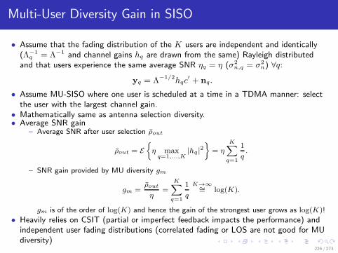
Multi-User Diversity Gain in SISO
• Assume that the fading distribution of the K users are independent and identically(Λ−1
q = Λ−1 and channel gains hq are drawn from the same) Rayleigh distributedand that users experience the same average SNR ηq = η (σ2
n,q = σ2n) ∀q:
yq = Λ−1/2hqc′ + nq.
• Assume MU-SISO where one user is scheduled at a time in a TDMA manner: selectthe user with the largest channel gain.
• Mathematically same as antenna selection diversity.• Average SNR gain
– Average SNR after user selection ρout
ρout = E
η maxq=1,...,K
|hq |2
= ηK∑
q=1
1
q.
– SNR gain provided by MU diversity gm
gm =ρout
η=
K∑
q=1
1
q
K→∞∼= log(K).
gm is of the order of log(K) and hence the gain of the strongest user grows as log(K)!
• Heavily relies on CSIT (partial or imperfect feedback impacts the performance) andindependent user fading distributions (correlated fading or LOS are not good for MUdiversity)
226 / 273

Multi-User Diversity Gain in SISO
• Sum-rate capacity
CTDMA = E CTDMA = E
log2
(
1 + η maxq=1,...,K
|hq |2)
.
– low SNR
CTDMA ≈ E
maxq=1,...,K
|hq|2
η log2 (e) ≈ gmCawgn.
Observations: capacity of the fading channel log(K) times larger than the AWGNcapacity.
– high SNR (Use Jensen’s inequality: Ex F (x) ≤ F (Ex x) if F concave)
CTDMA ≈ log2 (η) + E
log2
(
maxq=1,...,K
|hq |2)
,
≈ Cawgn + E
log2
(
maxq=1,...,K
|hq|2)
,
(a)
≤ Cawgn + log2
(
E
maxq=1,...,K
|hq|2)
,
= Cawgn + log2 (gm) .
Observations: capacity of a fading channel is larger than the AWGN capacity by afactor roughly equal to log2 (gm) ≈ log log (K).
• Fading channels are significantly more useful in a multi-user setting than in asingle-user setting
227 / 273

Multi-User Diversity
• In MU-MIMO, the performance is function of the channel magnitude but also of thespatial directions and properties of the channel matrices.
• MU diversity offers abundant spatial channel directions and allows to appropriatelychoose users with good channel matrix properties or spatial separations.
• Opportunistic Beamforming: precode multiple streams along the unitary precodingmatrix W (orthogonal beams). For a large number of users, thanks to MU diversity,each beam matches one user channel with a high probability and orthogonality ofbeams prevents users from experiencing multi-user interference
yq = Λ−1/2q hqWS
1/2c+ nq
K→∞= Λ−1/2
q ‖hq‖ s1/2q cq + nq.
– The terminal only measures the effective channel, i.e. the channel precoded by eachbeam, and reports the SNR (or CQI) for one or multiple beam(s).
– Works well only for very large K.
228 / 273
Multi-User Diversity
• Few fundamental differences with classical spatial/time/frequency diversity:– Diversity techniques, like space-time coding, mainly focus on improving reliability by
decreasing the outage probability in slow fading channels. MU diversity on the otherhand increases the data rate over time-varying channels.
– Classical diversity techniques mitigate fading while MU diversity exploits fading.
– MU diversity takes a system-level view while classical diversity approaches focus on asingle-link. This system-level view becomes increasingly important as we shift fromsingle-cell to multi-cell scenarios.
229 / 273

Resource Allocation, Fairness and Scheduling Criteria
• An appropriate scheduler should allocate resources (time, frequency, spatial, power)to the users in a fair manner while exploiting the MU diversity gain.
• Goal of the resource allocation strategy at the scheduler: maximize the utility metricU .
c′⋆,G⋆,K⋆
= arg max
c′,G,K⊂KU
where c′⋆ is the optimum transmit vector, G⋆ denotes the optimum set of receivebeamformers, and K⋆ ⊂ K refers to the optimum subset of users to be scheduled.
• Two major kinds of resource allocation strategies:– rate-maximization policy : maximizes the sum-rate - no fairness among users– fairness oriented policy, commonly relying on a proportional fair (PF) metric:
maximizes a weighted sum-rate and guarantees fairness among users.
• Those two strategies can be addressed by using two different utility metrics:
c′⋆,G⋆,K⋆ = arg max
c′,G,K⊂K
∑
q∈K
wqRq
where– rate-maximization approach: wq = 1
– proportional fair approach: wq =γqRq
(Rq is the long-term average rate of user q and
γq is the Quality of Service (QoS) of each user).
230 / 273

Practical Proportional Fair Scheduling
• The long-term average rate Rq of user q is updated using an exponentially weightedlow-pass filter such that the estimate of Rq at time k + 1, denoted as Rq (k + 1), isfunction of the long-term average rate Rq (k) and of the current rate Rq(k) atcurrent time instant k as outlined by
Rq (k + 1) =
(1− 1/tc) Rq (k) + 1/tcRq(k), q ∈ K⋆
(1− 1/tc) Rq (k) , q /∈ K⋆
where tc is the scheduling time scale and K⋆ refers to the scheduled user set at timek. The resources should thus be allocated at time instant k as
c′⋆,G⋆,K⋆
= arg max
c′,G,K⊂K
∑
q∈K
γqRq(k)
Rq(k).
• The scheduling time scale tc is a design parameter of the system that highlyinfluences the user fairness and the performance
– Very large tc: assuming all users experience identical fading statistics and have thesame QoS, the PF scheduler is equivalent to the rate-maximization scheduler, i.e. userscontributing to the highest sum-rate are selected.
– Small tc: assuming all users have the same QoS, the scheduler divides the availableresources equally among users (Round-Robin scheduling). No MU diversity is exploited.
231 / 273

Proportional Fair Scheduling
• Sum-rate of SISO TDMA with PF scheduling at SNR=0 dB as a function of thenumber of users K, the scheduling time scale tc and the channel model
hk = ǫhk−1 +√
1− ǫ2nk
with ǫ the channel time correlation coefficient.
0 10 20 30 40 500.8
1
1.2
1.4
1.6
1.8
2
2.2
2.4
2.6
Number of Users K
TD
MA
sum
−ra
te [b
ps/H
z]
ε=0.98ε=0.72ε=0
tc=1.1
tc=50
tc=1e4
232 / 273

User Grouping
• Given the presence of K users in the cell, the scheduler for MU-MIMO aims atfinding the best scheduled user set among all possible candidates within K.
• The exhaustive search is computationally intensive. Assuming a single streamtransmission per user and ne ≤ min nt,K, a search like (withR (K) =
∑
q∈KwqRq)
K⋆ = arg max
K⊂Kne≤minnt,K
R (K)
requires to consider a large number of different sets and has a complexity thatquickly becomes cumbersome as K increases.
233 / 273

Precoding with Perfect Transmit Channel Knowledge
• Single-link Spatial Multiplexing: Multiple Eigenmode Transmission relies on CSIknowledge at both the transmitter and the receiver and splits the spatial channelequalization between the transmitter and the receiver. As a result, the channel isdecoupled into multiple parallel data pipes.
• Unfortunately, this approach cannot be applied to MU-MIMO as the receivers do notcooperate.
• MIMO BC, DPC optimal but extremely complex. Any suboptimal strategies?• In MU-MIMO where CSI is available at the transmitter, precoding techniques
reminiscent of the receiver architectures for SM
precoding transmitter side receiver side
Linear Matched Beamforming (MBF) MRC
Linear Zero-Forcing Beamforming(ZFBF)
ZF
Linear Regularized Zero-Forcing Beamform-ing (R-ZFBF)
MMSE
Non-linear Tomlinson-Harashima Precoding(THP)
SIC
Non-linear Vector Perturbation (VP) sphere decoder
234 / 273

Achievable rate
• Maximum rate achievable by user q with linear precoding is
Rq =
nu,q∑
l=1
log2 (1 + ρq,l)
where ρq,l denotes the SINR experienced by stream l of user q
ρq,l =Λ−1
q |gq,lHqpq,l|2
Il + Ic + ‖gq,l‖2 σ2n,q
=Λ−1
q |gq,lHqwq,l|2 sq,lIl + Ic + ‖gq,l‖2 σ2
n,q
with pq,l = wq,lsq,l (resp. gq,l) the precoder (resp. combiner) attached to stream lof user q, Il the inter-stream interference and Ic the intra-cell interference (alsocalled multi-user interference)
Il =∑
m6=l
Λ−1q |gq,lHqpq,m|2 =
∑
m6=l
Λ−1q |gq,lHqwq,m|2 sq,m,
Ic =∑
p∈Kp 6=q
nu,p∑
m=1
Λ−1q |gq,lHqpp,m|2 =
∑
p∈Kp 6=q
nu,p∑
m=1
Λ−1q |gq,lHqwp,m|2 sp,m.
• If nr = 1, the SINR of user q simply reads as ρq =Λ−1q |hqwq |2sq
∑p∈Kp 6=q
Λ−1q |hqwp|2sp+σ2
n,q
.
235 / 273

Zero-Forcing Beamforming (ZFBF)
• Most popular MU-MIMO precoder. Assume single receive antenna per user.• Channel Direction Information (CDI) of user q: hq = hq/ ‖hq‖.• Idea is to force the intra-cell interference Ic to zero: the precoder of a user q, wq , is
chosen such that hpwq = 0 ∀p ∈ K \ q. Only possible if ne ≤ nt!• Define
H =[
Λ−1/2i h
Ti , . . . ,Λ
−1/2j h
Tj
]T
i,j∈K= DH
with
D = diag
Λ−1/2i ‖hi‖ , . . . ,Λ−1/2
j ‖hj‖
i,j∈K,
H =[
hTi , . . . , h
Tj
]T
i,j∈K.
The ZFBF aims at designing W = [wi, . . . ,wj ]i,j∈Ksuch that HW is diagonal.
• Assuming ne ≤ nt and H is full rank, the precoders can be chosen as the normalizedcolumns of the right pseudo inverse of H
F = HH(
HHH)−1
= FD−1 = H
H(
HHH)−1
D−1.
Transmit precoder wq for user q ∈ K: wq = F(:, q)/‖F(:, q)‖ = F(:, q)/‖F(:, q)‖where F(:, q) is to be viewed as the column of F corresponding to user q.
236 / 273

Zero-Forcing Beamforming (ZFBF)
• Assuming that c =[ci, . . . , cj
]T
i,j∈K, the received signal of user q ∈ K is
yq = Λ−1/2q hqwqs
1/2q cq + nq = dqcq + nq ,
with dq = Λ−1/2q hqwqs
1/2q = Λ
−1/2q
‖hq‖‖F(:,q)‖s
1/2q .
Observations: MU-MIMO channel with ZFBF is split into ne parallel(non-interfering) channels.
• The rate achievable by user q is given by
Rq = log2(1 + d2q/σ
2n,q
).
d2q is low if H is badly conditioned but would get larger if users’ CDI are orthogonalor quasi-orthogonal.
– reminiscent of the loss caused by noise enhancement incurred by the linear ZF
• For large K, better conditioning of matrix H through the use of user grouping.• By uniformly allocating the power across user streams sq = Es/ne and by choosing
ne = n = min nt,K, d2q/σ2n,q = α2
qηq/ne with α2q = |hqwq |2 = ‖hq‖2 /‖F(:, q)‖2
CBF (H) =
minnt,K∑
q=1
log2
(
1 + α2qηqn
)
.
At high SNR with ηq = η, CBF (H) ≈ min nt,K log2 (ηq). The multiplexing gainmin nt,K is achieved (same as with DPC).
237 / 273
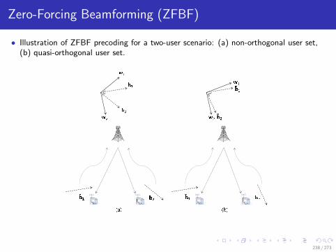
Zero-Forcing Beamforming (ZFBF)
• Illustration of ZFBF precoding for a two-user scenario: (a) non-orthogonal user set,(b) quasi-orthogonal user set.
238 / 273

Block Diagonalization (BD)
• Extension of ZFBF to multiple receive antennas and multiple streams per user.• Constraints on the transmit filters targeting user q ∈ K
Λ−1/2p HpWq = 0,∀p 6= q, p ∈ K
• Denoting Kq = K \ q of size Kq = ♯Kq, the interference space Hq ∈ CnrKq×nt is
Hq =[
. . . Λ−1/2p HT
p . . .]T
p∈Kq
.
• BD filter design forces Wq to lie in the null space of Hq : null space of Hq to bestrictly larger than 0 → r
(Hq
)< nt.
• An orthogonal basis of the null space of Hq is obtained by taking its SVD
Hq = UqΛq
[Vq V′
q
]H
where V′q refers to the eigenvectors of Hq associated with the null singular values.
• Assuming the zero-interference constraint is possible for all users in Kq and thatr(HqV
′q
)= nu,q , Wq writes as a linear combination of columns of V′
q as
Wq = V′qAq
with some nu,q × nu,q unitary matrix Aq.
239 / 273

Block Diagonalization (BD)
• Multi-user interference is eliminated and each user experiences an equivalentsingle-user MIMO channel Heq,q = HqV
′q, for which the optimal solution is obtained
by transmitting along the nu,q dominant right singular vectors of Heq,q
Heq,q =[Ueq,q U′
eq,q
][
Λeq,q 0
0 0
][Veq,q V′
eq,q
]H
where Veq,q refers to the nu,q dominant right singular vectors.• The final beamformer for user q writes as
Wq = V′qVeq,q .
• Applying Gq = UHeq,q , the equivalent channel of each user is
zq = Gqyq = Λ−1/2q Λeq,qS
1/2q cq +Gqnq.
• Achievable sum-rate (with λeq,q,m diagonal entries of Λ2eq,q)
∑
q∈K
nu,q∑
m=1
log2
(
1 + sq,mΛ−1
q λeq,q,m
σ2n,q
)
For a sum-power constraint∑
q∈K
∑nu,q
m=1 sq,m = Es, the optimal power allocation isobtained by water-filling.
240 / 273

Global Performance Comparison
• Sum-rate of linear (left) and non-linear (right) MU-MIMO precoders vs SNR innt = 4,K = 20 i.i.d. Rayleigh fading channels
−5 0 5 10 15 20 25 30 35 400
10
20
30
40
50
60
SNR [dB]
Sum
−ra
te [b
ps/H
z]
ZFWFgreedy−ZFWFMSRgreedy−MSRMSR−DE
−5 0 5 10 15 20 25 30 35 400
10
20
30
40
50
60
SNR [dB]
Sum
−ra
te [b
ps/H
z]
DPCMSR−DEgreedy−THPgreedy−ZFWFVP
Observations: ZFBF without user selection (ZFWF) performs poorly. ZFBF withuser selection (greedy-ZFWF) is a competitive strategy for MU-MIMO broadcastchannels, in terms of both performance and complexity.Keep in mind the assumptions: perfect CSIT, the same average SNR for all usersand a max-rate scheduler (i.e. there is no fairness issue involved here).
241 / 273
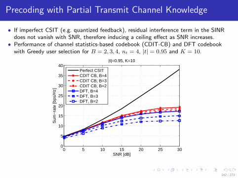
Precoding with Partial Transmit Channel Knowledge
• If imperfect CSIT (e.g. quantized feedback), residual interference term in the SINRdoes not vanish with SNR, therefore inducing a ceiling effect as SNR increases.
• Performance of channel statistics-based codebook (CDIT-CB) and DFT codebookwith Greedy user selection for B = 2, 3, 4, nt = 4, |t| = 0.95 and K = 10.
0 5 10 15 20 25 300
5
10
15
20
25
30
35
40|t|=0.95, K=10
SNR [dB]
Sum
−ra
te [b
ps/H
z]
Perfect CSITCDIT CB, B=4CDIT CB, B=3CDIT CB, B=2DFT, B=4DFT, B=3DFT, B=2
242 / 273

Introduction to Multi-Cell MIMO
243 / 273

Reference Book
• Bruno Clerckx and Claude Oestges, “MIMO Wireless Networks: Channels,Techniques and Standards for Multi-Antenna, Multi-User and Multi-Cell Systems,”Academic Press (Elsevier), Oxford, UK, Jan 2013.
– Chapter 13
Section: 13.1, 13.2, 13.3
244 / 273

Introduction
• Current wireless networks primarily operate using a frequency reuse 1 (or close to 1),i.e. all cells share the same frequency band
• Interference is not only made of intra-cell (i.e. multi-user interference), but also ofinter-cell (i.e. multi-cell) interference.
• Cell edge performance is primarily affected by the inter-cell interference.
245 / 273

Wideband/long-term SINR
• For user q in cell i, the wideband/long-term SINR is commonly evaluated by ignoringthe effect of fading but only account for path loss and shadowing
SINRw,q =Λ−1
q,iEs,i
σ2n,q +
∑
j 6=i Λ−1q,jEs,j
.
• Provides a rough estimate of the network performance. Function of majorpropagation mechanisms (path loss, shadowing, antenna radiation patterns,...), basestations deployment and user distribution.
• CDF of SINRw,q in a frequency reuse 1 network (cells share the same frequencyband) with 2D and 3D antenna patterns in urban macro deployment.
−10 −5 0 5 10 15 20 250
10
20
30
40
50
60
70
80
90
100
Downlink wideband SINR [dB]
CD
F [%
]
3D2D
246 / 273
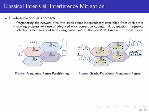
Classical Inter-Cell Interference Mitigation
• Divide-and-conquer approach:– fragmenting the network area into small zones independently controlled from each other– making progressively use of advanced error correction coding, link adaptation, frequency
selective scheduling and lately single-user and multi-user MIMO in each of those zones.
Figure: Frequency Reuse Partitioning. Figure: Static Fractional Frequency Reuse.
247 / 273
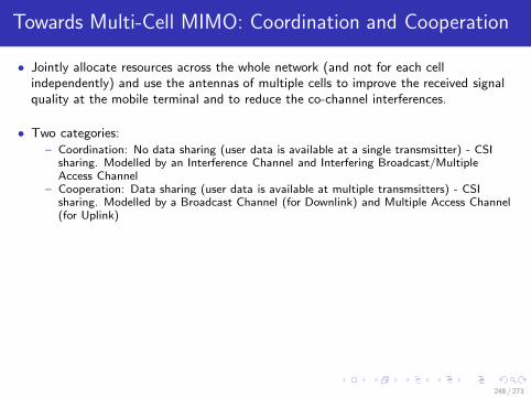
Towards Multi-Cell MIMO: Coordination and Cooperation
• Jointly allocate resources across the whole network (and not for each cellindependently) and use the antennas of multiple cells to improve the received signalquality at the mobile terminal and to reduce the co-channel interferences.
• Two categories:– Coordination: No data sharing (user data is available at a single transmsitter) - CSI
sharing. Modelled by an Interference Channel and Interfering Broadcast/MultipleAccess Channel
– Cooperation: Data sharing (user data is available at multiple transmsitters) - CSIsharing. Modelled by a Broadcast Channel (for Downlink) and Multiple Access Channel(for Uplink)
248 / 273
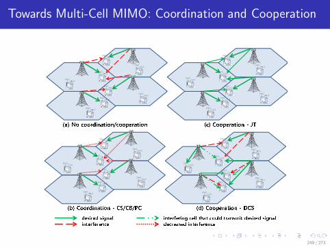
Towards Multi-Cell MIMO: Coordination and Cooperation
249 / 273
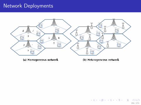
Network Deployments
250 / 273

System Model - Interference Channel
• Interfering (broadcast/multiple access) channel– For each transmitter i (one per cell), the intended receivers (i.e. users) are in cell i.– Each receiver (i.e. user) is only interested in what is being sent by the corresponding
transmitter.– Transmitters and receivers do not cooperate but only coordinate their transmissions by
sharing CSI information. In the downlink, one transmitter does not have access to thecodewords sent by other transmitters and cannot perform DPC. In the uplink, onereceiver never has access to other received signals and cannot perform SIC.
• General downlink multi-cell multi-user MIMO network with a total number of KT
users distributed in nc cells.• Ki users in every cell i, nt,i transmit antennas at BS i, nr,q receive antennas at
mobile terminal q.• The received signal of a given user q in cell i is
yq = Λ−1/2q,i Hq,ic
′i +∑
j 6=i
Λ−1/2q,j Hq,jc
′j
︸ ︷︷ ︸
inter-cell interference
+nq
where– yq ∈ Cnr,q ,– nq is a complex Gaussian noise CN
(0, σ2n,qInr,q
),
– Λ−1q,i refers to the path-loss and shadowing between transmitter i and user q,
– Hq,i ∈ Cnr,q×nt,i models the MIMO fading channel between transmitter i and user q.251 / 273
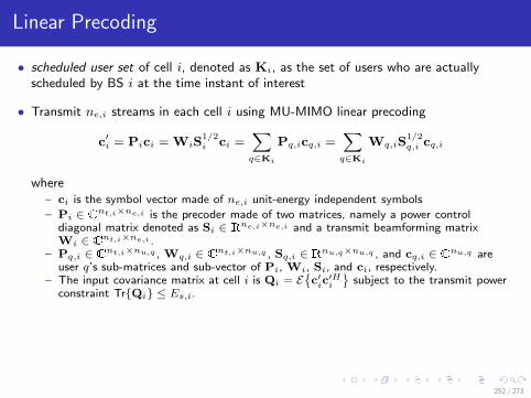
Linear Precoding
• scheduled user set of cell i, denoted as Ki, as the set of users who are actuallyscheduled by BS i at the time instant of interest
• Transmit ne,i streams in each cell i using MU-MIMO linear precoding
c′i = Pici = WiS
1/2i ci =
∑
q∈Ki
Pq,icq,i =∑
q∈Ki
Wq,iS1/2q,i cq,i
where– ci is the symbol vector made of ne,i unit-energy independent symbols
– Pi ∈ Cnt,i×ne,i is the precoder made of two matrices, namely a power controldiagonal matrix denoted as Si ∈ Rne,i×ne,i and a transmit beamforming matrixWi ∈ Cnt,i×ne,i .
– Pq,i ∈ Cnt,i×nu,q , Wq,i ∈ Cnt,i×nu,q , Sq,i ∈ Rnu,q×nu,q , and cq,i ∈ Cnu,q areuser q’s sub-matrices and sub-vector of Pi, Wi, Si, and ci, respectively.
– The input covariance matrix at cell i is Qi = Ec′ic
′Hi
subject to the transmit power
constraint TrQi ≤ Es,i.
252 / 273

Linear Precoding
• The received signal yq ∈ Cnr,q of user q ∈ Ki
yq = Λ−1/2q,i Hq,iPq,icq,i +
∑
p∈Ki, p 6=q
Λ−1/2q,i Hq,iPp,icp,i
︸ ︷︷ ︸
intra-cell (multi-user) interference
+∑
j 6=i
∑
l∈Kj
Λ−1/2q,j Hq,jPl,jcl,j
︸ ︷︷ ︸
inter-cell interference
+nq.
• Apply a receive combiner to stream l of user q in cell i
zq,l = gq,lyq = Λ−1/2q,i gq,lHq,ipq,i,lcq,i,l +
∑
m6=l
Λ−1/2q,i gq,lHq,ipq,i,mcq,i,m
︸ ︷︷ ︸
inter-stream interference
+∑
p∈Ki, p 6=q
Λ−1/2q,i gq,lHq,iPp,icp,i
︸ ︷︷ ︸
intra-cell (multi-user) interference
+∑
j 6=i
∑
l∈Kj
Λ−1/2q,j gq,lHq,jPl,jcl,j
︸ ︷︷ ︸
inter-cell interference
+gq,lnq.
253 / 273

Achievable Rate
• By treating all interference as noise, the maximum rate achievable by user q in cell iwith linear precoding is
Rq,i =
nu,q∑
l=1
log2 (1 + ρq,l) .
• The quantity ρq,l denotes the SINR experienced by stream l of user-q and writes as
ρq,l =S
Il + Ic + Io + ‖gq,l‖2 σ2n,q
.
where S refers to the received signal power of the intended stream, Il theinter-stream interference, Ic the intra-cell interference (i.e. interference fromco-scheduled users) and Io the inter-cell interference and they write as
S = Λ−1q,i |gq,lHq,ipq,i,l|2 ,
Il =∑
m6=l
Λ−1q,i |gq,lHq,ipq,i,m|2 ,
Ic =∑
p∈Ki,p 6=q
nu,p∑
m=1
Λ−1q,i |gq,lHq,ipp,i,m|2 ,
Io =∑
j 6=i
Λ−1q,j ‖gq,lHq,jPj‖2 .
254 / 273
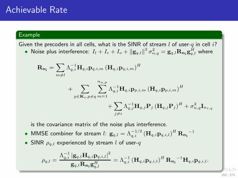
Achievable Rate
Example
Given the precoders in all cells, what is the SINR of stream l of user-q in cell i?• Noise plus interference: Il + Ic + Io + ‖gq,l‖2 σ2
n,q = gq,lRnigHq,l where
Rni=∑
m6=l
Λ−1q,iHq,ipq,i,m (Hq,ipq,i,m)H
+∑
p∈Ki,p 6=q
nu,p∑
m=1
Λ−1q,iHq,ipp,i,m (Hq,ipp,i,m)H
+∑
j 6=i
Λ−1q,jHq,jPj (Hq,jPj)
H + σ2n,qInr,q
is the covariance matrix of the noise plus interference.
• MMSE combiner for stream l: gq,l = Λ−1/2q,i (Hq,ipq,i,l)
HRni
−1
• SINR ρq,l experienced by stream l of user-q
ρq,l =Λ−1
q,i |gq,lHq,ipq,i,l|2
gq,lRnigHq,l
= Λ−1q,i (Hq,ipq,i,l)
HRni
−1Hq,ipq,i,l.
255 / 273
Capacity of the Interference Channel
256 / 273

Reference Book
• Bruno Clerckx and Claude Oestges, “MIMO Wireless Networks: Channels,Techniques and Standards for Multi-Antenna, Multi-User and Multi-Cell Systems,”Academic Press (Elsevier), Oxford, UK, Jan 2013.
– Chapter 13
Section: 13.4
257 / 273

SISO Interference Channel
• What is the capacity region of the two-user SISO IC?
• ηq,i = Λ−1q,iEs,i/σ
2n,q
– long-term SNR when user q is served by cell i– long-term INR (interference to noise ratio) when q is a victim user of cell i
• ηq,i = ηq,i |hq,i|2 can be thought of as an instantaneous SNR or INR
• two-user SISO IC: transmitter 1 (i.e. cell 1) communicates with user 1 andtransmitter 2 (i.e. cell 2) with user 2
– achievable rate region function of η1,1, η2,2, η1,2, η2,1– symmetric SISO IC characterized by η1,1 = η2,2 = ηd and η1,2 = η2,1 = ηc– symmetric rate: Rsym = max(R1,R2)∈CIC
min R1, R2 where R1 and R2 are therates achievable by user 1 and 2 respectively in the two-user SISO IC and CIC is thecapacity region of the SISO IC
258 / 273

Degrees of Freedom - Multiplexing Gain
Figure: Achievable multiplexing gain per user of the two-user Gaussian SISO IC (α = INR/SNR).
259 / 273

Very Strong Interference Regime
• Can the capacity region, under some interference conditions, become a square onlydetermined by the inequalities Ri ≤ log2 (1 + ηi,i) , i = 1, 2?
– i.e. each transmitter can communicate with its receiver at a rate equal to the oneachievable without any interference
• Very strong interference regime conditions: η1,2 ≥ η2,2 + η1,1η2,2 andη2,1 ≥ η1,1 + η1,1η2,2
• The interference is so strong that each user performs SIC by decoding the interferingmessage first and subtracting it from the received signal before decoding its ownmessage.
• Each transmitter can communicate with its receiver at a rate Ri = log2(1 + ηi,i
)for
i = 1, 2, as in the absence of any interference.• The symmetric rate (symmetric capacity) simply writes as
Rsym = log2 (1 + ηd) .
260 / 273

Very Strong Interference Regime
• The very strong interference conditions can be viewed from an angle that isreminiscent of the SIC behavior in SISO BC.
• When user 1 decodes user 2’s signal in the very strong interference regime, it treatsits own signal as noise. Hence, for user 1 to be able to cancel correctly user 2’ssignal, the interfering channel between transmitter 2 and user 1 has to be strongenough to support R2, i.e.
R2 ≤ log2
(
1 +Λ−1
1,2 |h1,2|2 Es,2
σ2n,1 + Λ−1
1,1 |h1,1|2 Es,1
)
= log2
(
1 +η1,2
1 + η1,1
)
.
Given that user 2 wants to receive its message at a rate R2 = log2(1 + η2,2
), this
puts the constraints
log2(1 + η2,2
)≤ log2
(
1 +η1,2
1 + η1,1
)
,
which equivalently writes as η1,2 ≥ η2,2 + η1,1η2,2. The other condition is obtainedsimilarly by looking at user 2’s requirement to decode user 1’s message correctly.
261 / 273

Real-World MIMO Wireless Networks
262 / 273

Reference Book
• Bruno Clerckx and Claude Oestges, “MIMO Wireless Networks: Channels,Techniques and Standards for Multi-Antenna, Multi-User and Multi-Cell Systems,”Academic Press (Elsevier), Oxford, UK, Jan 2013.
– Chapter 14
263 / 273

System Requirements
• peak rate– highest theoretical throughput achievable with SU-MIMO spatial multiplexing but are
typically not achieved in practical deployments.– e.g. 8x8 Spatial multiplexing with 8 streams transmission
• cell average spectral efficiency– average spectral efficiency of a cell (with K users).– much more representative of throughput encountered in practice
• cell edge user spectral efficiency– spectral efficiency achieved by at least 95% of the users in the network.– much more representative of throughput encountered in practice
264 / 273

Frame Structure
• Multiplexing/Access– DL: OFDM– UL: DFT-Spread OFDM (SC-FDM)
• Frame structure– OFDMA/SC-FDMA create a
time-frequency grid composed oftime-frequency resources
– A resource block (RB) is formed by 12consecutive REs in the frequencydomain for a duration of 7 OFDMsymbols in the time domain.
– A subframe is formed of 14consecutive OFDM/SC-FDM symbols.
– Scheduling and data transmission isperformed at the RB-level with theminimum scheduling unit consisting oftwo RBs within one subframe.
– First 3 symbols used to carry controlinformation.
265 / 273

Key Downlink Technologies
• Antenna configurations: 2, 4 or 8 transmit antennas and a minimum of 2 receiveantennas
• LTE Rel. 8 (finalized in Dec 2008):– Up to 4x4 (up to 4 stream transmission)– Transmit diversity (to protect against fading) using Orthogonal Space-Frequency Block
Coding (O-SFBC) for 2Tx, non-orthogonal SFBC for 4TX– Open-loop (for high speed) Spatial Multiplexing with rank adaptation based on
predefined precoders– Closed-loop (for low speed) Spatial Multiplexing based on codebook precoding– Stone-age MU-MIMO based on common reference signals (CRS)
• LTE Rel. 9 (finalized in Dec 2009):– Up to 4x4 (up to 4 stream transmission)– Introduction of demodulation reference signals (DM-RS)– Enhancement of MU-MIMO to support ZFBF-like precoding
• LTE-A Rel. 10 (finalized mid 2011):– Up to 8x8 (up to 8 stream transmission)– New channel measurement reference signals (CSI-RS)– New feedback mechanisms for 8Tx (dual codebook W1W2 structure)– HetNet - eICIC
• LTE-A Rel. 11 (finalized in Dec 2012):– Coordinated Multi-Point Transmission/Reception (CoMP) for Homogeneous (Macro)
and heterogeneous (pico, DAS) networksDynamic cell/point selection combined with dynamic ON/OFF blanking
266 / 273

Key Uplink Technologies
• Antenna configurations: 1, 2 or 4 transmit antennas in the uplink with a minimum of2 receive antennas
• LTE Rel. 8 (finalized in Dec 2008):– single antenna transmission and transmit antenna selection– MU-MIMO
• LTE-A Rel. 10 (finalized mid 2011):– Spatial Multiplexing with codebook– Transmit diversity (for control channels)
• LTE-A Rel. 11 (finalized in Dec 2012):– Coordinated Multi-Point Transmission/Reception (CoMP)
267 / 273
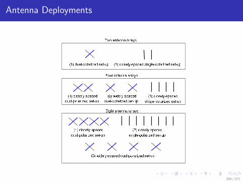
Antenna Deployments
268 / 273

Reference Signals
Dedicated RS (DRS) Common RS (CRS)
For demodulation For demodulation and measurement
Targets a specific terminal Shared among a group of terminals
Terminal specifically precoded Commonly non-precoded
Overhead proportional to the numberof transmitted streams
Overhead proportional to the numberof transmit antennas
Sent in RBs where data is present Sent in all RBs
Channel estimation less flexible Channel estimation more flexible
269 / 273

Reference Signals
270 / 273

Channel State Information (CSI) feedback
• Three main feedback information:– Rank Indicator (RI): the preferred number of streams (denoted as layers in LTE) a user
would like to receive– Precoding Matrix Indicator (PMI): the preferred precoder in the codebook– Channel Quality Indicator (CQI): the rate achievable with each stream (used to
perform link adaptation)
• Open-Loop relies only on RI and CQI– High mobility or limited CSI feedback prevent the use of PMI
• Closed-Loop (Spatial Multiplexing and MU-MIMO) rely on RI, CQI and PMI– If Spatial Multiplexing, the actual precoder is the same as the one selected by the user
(PMI)– If MU-MIMO based on CRS, the actual precoder is the same as the one selected by the
user (PMI)– If MU-MIMO based on DM-RS, the actual precoder (e.g. ZFBF) is computed based on
the one selected by the user (PMI).
271 / 273

Network Deployments
272 / 273

Beyond LTE-A: Massive Multi-Cell and MassiveMulti-Antenna Networks
273 / 273


![NL 5 Beatrix Clerckx [Read-Only] - fresubin.be · Cumulative proportion weaned alive from MV Cumulative proportion discharged alive from ICU Cumulative proportion discharged alive](https://static.fdocuments.in/doc/165x107/5d03708c88c9936e148b4f75/nl-5-beatrix-clerckx-read-only-cumulative-proportion-weaned-alive-from-mv.jpg)