Ecosyste m Mode lling Pa ge 1

Vladimir I. Zvalinsky

PICES 2005

Ema il:

The ecosystem parameters and its stability. Theoretical consideration

V.I.Il'ichev Pacific Oceanological Institute, Far Eastern Branch, Russian Academy of Sciences,

Vladivostok, 690041, Russia

viz@poi.dvo.ru

Ecosyste m Mode lling Page 2

USUALEc osyste m mod e lling oc curs a s fo llow:- Mo de lling o f e a c h se pa ra te trop hic link;- Co nne ction o f trophic link be twe en e a c h othe r;- Attributing o f some laws for connec tio n o f links.

NEMURO MODEL 2000 is the e xa mple o f such proc edure .In result we ha ve no t a bso lute ly e co system, but c onnec ted amo ng the mse lve s diffe re nt tro phic links.At such ap proa ch e co system pa rame te rs, a s a whole , may not be re ve a le d.

PICES 2005

Ec osyste m mode lling Pa ge 3

ANOTHER WAY

- At first the e c osyste m c once ptua l mo de l is de signe d;- Then the la w o f transition substanc e from o ne trophic link to anothe r (or the c onc eptua l mod e l o f sep ara te link) is de sig ne d;- Formula tion o f full se t of equations;- Red uce the se t o f e qua tio ns to d ime nsionless fo rm a nd a na lysis.

As an example the six compartment e cosyste m mode l is consid ere d.

PICES 2005

Sedi

men

tatio

nLight

In

ZL

I

Mortality

Egestion

Inorganic matter

incorporationG

razing

Grazing

Respiration

Mineralisation

Ph

Exchange

E-cycleTransition

law

Transition law

Transition law

Tran

sition

law

Transition law

Conceptual model of ecosystem as ecological cycleEcosystem represents by 6 compartments. Four of them are livinglinks (Phy, SZ, LZ and Bacterial) and two of them are non living ones(inorganic matter and detritus).

Page 4

PICES 2005

Det

ZS

B

5

6

C5Solar light

Herbi-vores

Carnivores

Bacte-rium

Detritus

Phyto-plank- ton

Primaryproduction4

3

C1

C2C

C

C0

I

Respiration

Sedimentation

Vertical

exchange

MortalityEgestion

PP

ZS

ZL

B

rEB rEP

rES

rEL

Vij

C5

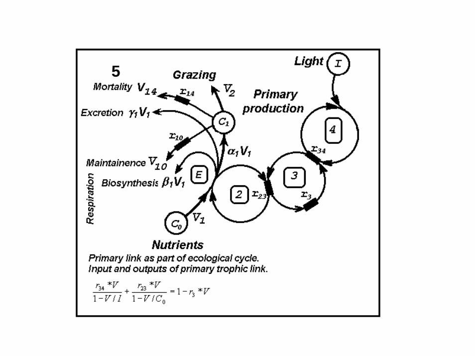
Ecosystem as a system of coupled cyclical processesEcosystem parameters

rP2rP1

rS1rS2

rB2

rL2rL1

rB1

rP

B2rrB1+R =B

rS2rS1 +R =ZS

rL2rL1 +R =ZL

r rP2 PrP1 + +R =PP

E

RBRZS R ZLRPP, , ,

C +0C =tot C +3 C5C +1 C +2 C +4

- total resistance of each trophic link

- total concentration of limiting nutrient

rEPrEB rES rEL, , , - coupling resistance between ecosystem cycle and each trophic link

7

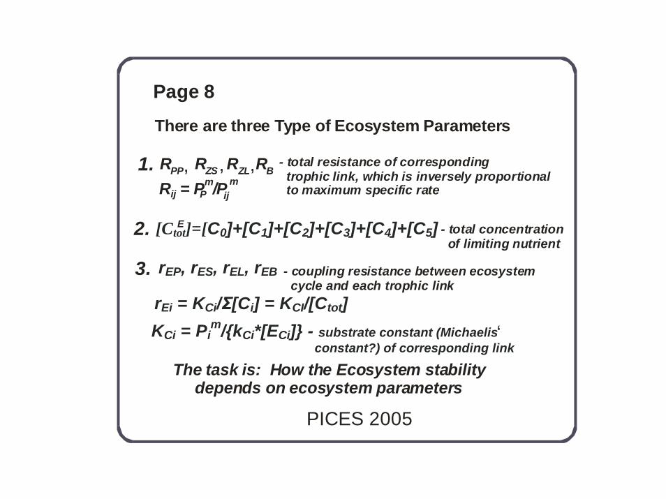
There are three Type of Ecosystem Parameters

RBRZS R ZLRPP, , ,

E

mmR = P /Pij P ij

- total resistance of corresponding trophic link, which is inversely proportional to maximum specific rate

- total concentration of limiting nutrient

- coupling resistance between ecosystem cycle and each trophic link

[Ctot]=[C0]+[C1]+[C2]+[C3]+[C4]+[C5]

1.

2.

3.

KCi = Pim/{kCi*[ECi]} - substrate constant (Michaelis

constant?) of corresponding link

rEP, rES, rEL, rEB

rEi = KCi/Σ[Ci] = KCI/[Ctot]

Page 8

PICES 2005

‘

The task is: How the Ecosystem stability depends on ecosystem parameters

Page 9

PICES 2005

0 2 4 6Substrate concentration, S=[S]/KC

0

0.2

0.4

0.6

0.8

1

Proc

ess

rela

tive

rate

, V=P

/Pm

M-M

g=0.80.95BL

tanh

exp

KC

Different kinetic curves for description of biological process what most often are using.Change of the factor hyperbola non-rectangularity "g" from "0.0" up to "1.0" changes the curve shape from "M-M" variant up to "Blackman" one.

g=0.0g=0.

999

0 2 4 6Substrate concentration, S=[S]/KC

0

0.2

0.4

0.6

0.8

1

M-M

0.95BL

KC

We used two kinetic curves: M-M curve (g=0.0) and curve with factor g=0.95 (which close to BL and close to experimental kinetic curves.

g=0.0g=0.

999

Page 10Parameters combination used for execution of

ecosystem behavior

Parameters I II III IV

RPP 1.0 1.0 1.0 1.0

RZS 2.0 2.0 4.0 4.0

RZL 4.0 4.0 8.0 8.0

Factor "g" 0.0 0.0 0.95 0.95

rEP=rES=rEL V a r i a b l e s

Time course of primary link at different rE Page 11

g=0.0 (M-M kinetics); rPP=1; rZS=2; rZL=4

0 100 200 300 400 500Time, in 1/Pm (=days)

0

0.2

0.4

0.6

0.8Co

ncen

trat

ion

C Ph

Nemuro, g=0.0 (M-M); rPP=1; rZS=2; rZL=4

rE=1

rE=0.5

rE=2

rE=KC/[Ctot]L

Decreasing of rE (increasing of [Ctot]L) causes oscillations

rE=0.4

At Ctot=2*KC (rE=0.5) - undamped Osc.

The same time course, but g=0.95 Page 12(BL kinetics); at rE < 0.5 - undamped oscillation At such kinetics of each process less amplitude oscillations

0 100 200 300 400 500Time, in 1/Pm (=days)

0

0.2

0.4

0.6

0.8

Conc

entr

atio

n C P

h

rE=1

rE=0.3

rE=0.5

rE=2

rE=0.19

rE=0.17rE=KC/[Ctot]L

Time course of primary link at different rE Page 13g=0.0 (M-M kinetics); rPP=1; but rZS=4; rZL=8

More amlitude oscillations, more period

0 200 400 600 800 1000Time, in 1/Pm (=days)

0

0.2

0.4

0.6

0.8

Conc

entr

atio

n C P

h

rE=1

rE=0.5

rE=2

rE=0.4

At Ctot=KC (rE=1.0) - undamped Osc.

The same time course, but g=0.95 Page 14(BL kinetics); at rE < 0.5 - undamped oscillation

At such kinetics of each process less amplitude oscillations

0 200 400 600 800 1000Time, in 1/Pm (=days)

0

0.2

0.4

0.6

0.8

Conc

entr

atio

n C P

h

rE=0.5

rE=2

rE=1(4:8)

rE=0.37

Page 15

• Michaelis-Menten not steep kinetics of each biological process couses higher amplitude oscillation at less total concentration ecosystem limiting nutrient

• Steep kinetics (close to Blackman’s broken line) couses less amplitude oscillation at higher total concentration ecosystem limiting nutrient

• Higher difference between specific rate growth of neighboring trophic links couses higher amplitude of oscillations with higher period

Very high period of oscillations shows the non biological nature of oscillations. The Czs equal to 0.0 for a long time? We think that this is impossible in Nature. It must be some Threshold for min C. We introduce threshold.

Page 16

0 100 200 300 400 500Time, in 1/Pm (=days)

0

0.2

0.4

0.6

0.8

Con

cent

ratio

n C

Ph, C

ZS, C

ZL

rE=0.5 CPh

CZS

CZL

It is very high period of oscillations

g=0.0 (M-M); rPP=1; rZS=2; rZL=4

Dinamics of the same ecosystem at introducing Page 17of Threshold = 0.1*rE = 0.1*Kc. No oscillations. Real time relaxation.

More steep kinetic curve (g=0.95) - less time relaxation

0 40 80 120 160Time, in 1/Pm (=days)

0

0.2

0.4

0.6

Con

cent

ratio

n C

Ph, C

ZS, C

ZL

CPh

CZS

g=0.0

g=0.95

g=0.95 g=0.0

Whith threshold of Ci at M-M kinetic curve (g=0.0) Page 18it is possible to find special ratio of rEi, when oscillations take place: rEP=0.7; rES=0.13; rEL=0.9. But at steep kinetic curve (g=0.95) there are no oscillation at any rEi.

0 40 80 120 160 200Time, in 1/Pm (=days)

0

0.2

0.4

Conc

entr

atio

n C P

h

Tresh=0.05

g=0.

95 g=0.

0

g=0.

0Tr

esh=

0.1

Page 19Conclusion

• In order to construct the predictive ecosystem model we must to understand the essential inner attributes of marine ecosystem.

• For the ecosystem modelling it is necessary to reveal mathematical couses of ecosystem stability/unstability from the biological and ecological ones and divide them from each other.

• On PICES 2001 Ken Denman said: «Stability of simple Box Model is ‘Fragile’»

• Our knowlidge about marine ecosystem is not less ‘Fragile’