Economics Lecture 9 - Univerzita Karlovavitali/documentsCourses... · • A firm is a price taker...
104
Economics Lecture 9 2016-17 Sebastiano Vitali
Transcript of Economics Lecture 9 - Univerzita Karlovavitali/documentsCourses... · • A firm is a price taker...

Economics Lecture 9
2016-17
Sebastiano Vitali

Course Outline
1 Consumer theory and its applications1.1 Preferences and utility
1.2 Utility maximization and uncompensated demand
1.3 Expenditure minimization and compensated demand
1.4 Price changes and welfare
1.5 Labour supply, taxes and benefits
1.6 Saving and borrowing

2 Firms, costs and profit maximization
2.1 Firms and costs
2.2 Profit maximization and costs for a price taking firm
3. Industrial organization
3.1 Perfect competition and monopoly
3.2 Oligopoly and games

2.2 Profit maximization
and costs for a price
taking firm

2.2 Profit maximization and costs for a price
taking firm1. Definition of price taking
2. The shutdown and output rules
3. Profit maximization by a price taking CRS firm
4. Cost curves, profit maximization and supply with
decreasing returns to scale
5. Cost curves with increasing returns to scale
6. Cost curves and supply with a u-shaped average cost curve
7. Long run and short run costs and supply

1. Definition of price taking
A firm is a price taker if nothing it can do affects the prices it
pays for inputs and outputs.
In particular its output quantity does not affect its output price.
Price taking does not mean prices do not change, just they do
not change because of the firm will.
Price taking is plausible if the firm has a small market share.

2. The shutdown & output
rules

2. The shutdown & output rules
),,( profits
),,(cost total, revenue
AC cost, average is ),,(
so
cost totalis ),,(
qwvcpq
qwvcpq
q
qwvc
qwvc
Why we need to know
about average costs.
The shutdown rule and average cost.

AC ),,(
p
so 0),,( profits
0at profits maximizes firm theif so 0 producing
by profits 0 makecan firm the
0)0,,( i.e. 0, is 0 producing ofcost theIf
q
qwvc
qwvcpq
q
wvc
The shutdown rule
Why we need to know
about average costs.

AC. price then 0 q produces
firm maximisingprofit a if
that implies ruledown shut The
output. of levels allat AC price if
produce)not (doesdown shuts firm The
The shutdown rule

The output rule and marginal cost
profits. decreases output increasingthen
cost marginal cR
revenue marginal If
profits. increases output increasingthen
cost marginal cR
revenue marginal If
q)w,c(v, - R(q) cost - revenue Profit
q
q

The output rule and marginal cost
shortly. thisof examplean see You will
on.maximizatiprofit imply y necessarilnot does
cost marginal revenue marginalBut
cost. marginal cR
revenue marginal
implies 0 qat on maximizatiProfit
Why we
need to know
about
marginal
costs.

What is marginal revenue?
• By definition for a price taking firm
marginal revenue = price
and does not vary with output
(note that perfect competition implies price taking)
• For a monopoly marginal revenue depends on the firm’s
output
• For a firm in an oligopoly marginal revenue depends on
the firm’s output & the output of other firms.

The relationship between
marginal cost &
average cost

O q1 q
€
Total cost c(v,w,q).
Total marginal and average costs
c1
Average cost at q1
= c1/q1
= gradient of chord OA Marginal
cost at q1 =
gradient of
tangent
A

O q1 q
€
Total cost c(v,w,q).
Total marginal and average costs
c1
Average cost at q1
= c1/q1
= gradient of chord OA Marginal
cost at q1 =
gradient of
tangent
A

O q1 q
£
Total cost c(v,w,q).
Total marginal and average costs
c1
Average cost at q1
= c1/q1
= gradient of chord OA Marginal
cost at q1 =
gradient of
tangent
A

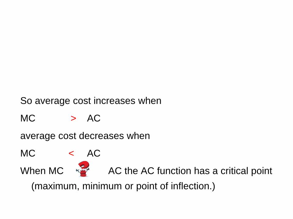
So average cost increases when
MC > AC
average cost decreases when
MC < AC
When MC = AC the AC function has a critical point
(maximum, minimum or point of inflection.)

So average cost increases when
MC > AC
average cost decreases when
MC < AC
When MC = AC the AC function has a critical point
(maximum, minimum or point of inflection.)
So average cost increases when
MC > AC
average cost decreases when
MC < AC
When MC = AC the AC function has a critical point
(maximum, minimum or point of inflection.)

So average cost increases when
MC > AC
average cost decreases when
MC < AC
When MC = AC the AC function has a critical point
(maximum, minimum or point of inflection.)

3. Profit maximization by
a price taking for a
constant returns to scale
(CRS) firm

3. Profit maximization by a price taking CRS
firm
The production function
q = f(K,L) has constant returns
to scale if
for all positive numbers m
mf(L,K) = f(mL,mK).
0 L
K
isoquants with CRS
q = 1
q = 2
q = 3
Cost curves with CRS

Under constant returns to scale CRS the optimal ratio of
inputs (e.g. the capital labour ratio)
is the same at all levels of output.
Multiplying inputs by 2 multiplies output by 2.
So it costs twice as much to produce 2 units of output as it
costs to produce 1 unit of output.
More generally with constant returns to scale, given input
prices v and w
c(v,w,mq) = mc(v,w,q).

Marginal cost = average cost
vary with input prices v and w but not with output
Total cost function from a CRS
production function
c(v,w,q),
gradient = MC = AC
€
0 output q

0 output q
Marginal and average cost from
a CRS production function
c = MC = AC
Marginal cost = average cost =c
varies with input prices v and w but not with output
€/unit
c

• A firm is a price taker if nothing it can do changes the
price p at which it sells.
• Profits = pq – cq = (p – c)q
• If p > c, so (p – c) > 0 increasing q always increases
profits, there is no profit maximizing output.
• If p < c so (p – c) < 0 the firm makes losses at all q > 0 so
produces 0.
• If p = c the firm makes 0 profit at any q.
p = c is the only price at which a price taking firm with
constant returns to scale has a profit maximum at q > 0.

4.Cost curves profit
maximization & supply
with decreasing returns
to scale

Under decreasing returns to scale DRS multiplying inputs
by 2 multiplies output by than 2.
So it costs than twice as much to produce 2 units of
output as it costs to produce 1 unit of output, so
c(v,w,2q) 2c(v,w,q).
4. Cost curves, profit maximization and supply
with decreasing returns to scale

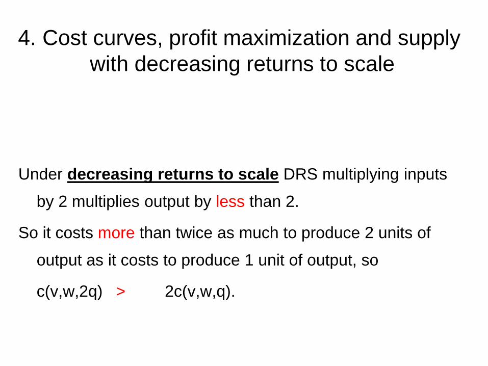
Under decreasing returns to scale DRS multiplying inputs
by 2 multiplies output by less than 2.
So it costs more than twice as much to produce 2 units of
output as it costs to produce 1 unit of output, so
c(v,w,2q) 2c(v,w,q).
4. Cost curves, profit maximization and supply
with decreasing returns to scale
Under decreasing returns to scale DRS multiplying inputs
by 2 multiplies output by less than 2.
So it costs more than twice as much to produce 2 units of
output as it costs to produce 1 unit of output, so
c(v,w,2q) > 2c(v,w,q).
4. Cost curves, profit maximization and supply
with decreasing returns to scale

More generally with decreasing returns to scale, given input
prices if m > 1
c(v,w,mq) > m c(v,w,q)
so AC at output mq = c(v,w,mq) c(v,w,q) = AC output q
mq q
AC with output.
Cost curves with DRS

More generally with decreasing returns to scale, given input
prices if m > 1
c(v,w,mq) > m c(v,w,q)
so AC at output mq = c(v,w,mq) > c(v,w,q) = AC output q
mq q
AC increases with output.
Cost curves with DRS
€
0 1 2 output q
Total cost function from a DRS
production function
MC = gradient of tangent AC = gradient of chord.
MC as q increases.
AC as q increases.
MC AC.

€
0 1 2 output q
Total cost function from a DRS
production function
MC = gradient of tangent AC = gradient of chord.
MC increases as q increases.
AC as q increases.
MC AC.

€
0 1 2 output q
Total cost function from a DRS
production function
MC = gradient of tangent AC = gradient of chord.
MC increases as q increases.
AC increases as q increases.
MC AC.

€
0 1 2 output q
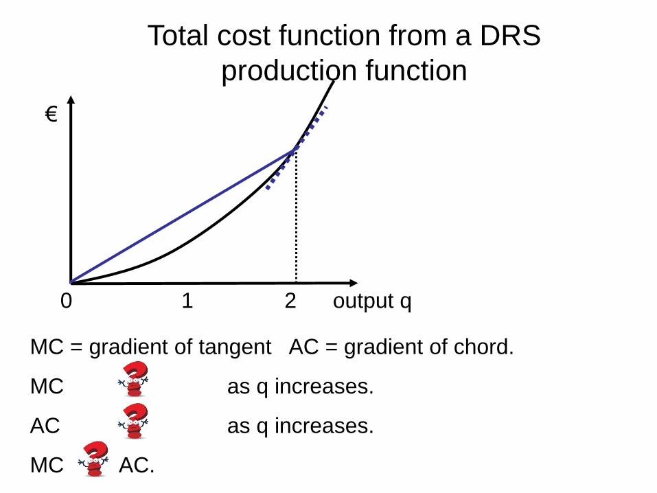
Total cost function from a DRS
production function
MC = gradient of tangent AC = gradient of chord.
MC increases as q increases.
AC increases as q increases.
MC > AC.

0 q
MC
AC
MC AC
everywhere
MC
as q increases
AC
as q increases
AC and MC from a DRS production function.
€/unit

0 q
MC
AC
MC > AC
everywhere
MC
as q increases
AC
as q increases
AC and MC from a DRS production function.
€/unit

0 q
MC
AC
MC > AC
everywhere
MC increases
as q increases
AC
as q increases
AC and MC from a DRS production function.
€/unit

0 q
MC
AC
MC > AC
everywhere
MC increases
as q increases
AC increases as
q increases
AC and MC from a DRS production function.
€/unit

€/unit
0 q1 output q
MC
p*
When q < q1 MC < p*, increasing output by 1 unit increases
costs by MC and revenue by p*. As p* > MC this increases
profits.
When q > q1 MC > p*, increasing output by 1 unit increases
costs by MC and revenue by p*. As p* < MC this decreases
profits.
If MC is increasing p = MC gives a profit
maximum: intuition

If MC is increasing p = MC gives a profit
maximum: calculus
π(q) = pq – c(q) ( c(q) = total cost )
First order condition for profit maximization
π’(q) = p – c’(q) = price – marginal cost = 0.
As c’’(q) is the derivative of c’(q) = MC increasing marginal
cost implies that c’’(q) > 0
The second derivative π’’(q) = – c’’(q) < 0 so
π(q) = pq – c(q) is a concave function of q.
The first order conditions give a maximum.

0 q* q
MC =
supply
AC
€/unit
Profit maximization with price taking and a
DRS production function
p
With DRS MC is increasing and MC > AC
If p = MC then p > AC so the shutdown rule is satisfied.
The MC curve is the supply curve. The firm makes profits.

5. Cost curves profit
maximization & supply
with increasing returns
to scale

Under increasing returns to scale IRS multiplying inputs by 2
multiplies output by more than 2.
So it costs less than twice as much to produce 2 units of
output as it costs to produce 1 unit of output, so
c(v,w,2q) < 2c(v,w,q).
More generally with increasing returns to scale, given input
prices if m > 1
c(v,w,mq) < m c(v,w,q)
so AC at output mq = c(v,w,mq) < c(v,w,q) = AC at output q
mq q
AC decreases with output.
5. Cost curves with IRS

€
0 1 2 output q
Total cost function from an IRS
production function
MC = gradient of tangent < AC = gradient of chord

€
0 1 2 output q
Total cost function from an IRS
production function
MC decreases as q increases

€
0 1 2 output q
Total cost function from an IRS
production function
MC decreases as q increases

€
0 1 2 output q
Total cost function from an IRS
production function
AC decreases as q increases,
there are economies of scale

€
0 1 2 output q
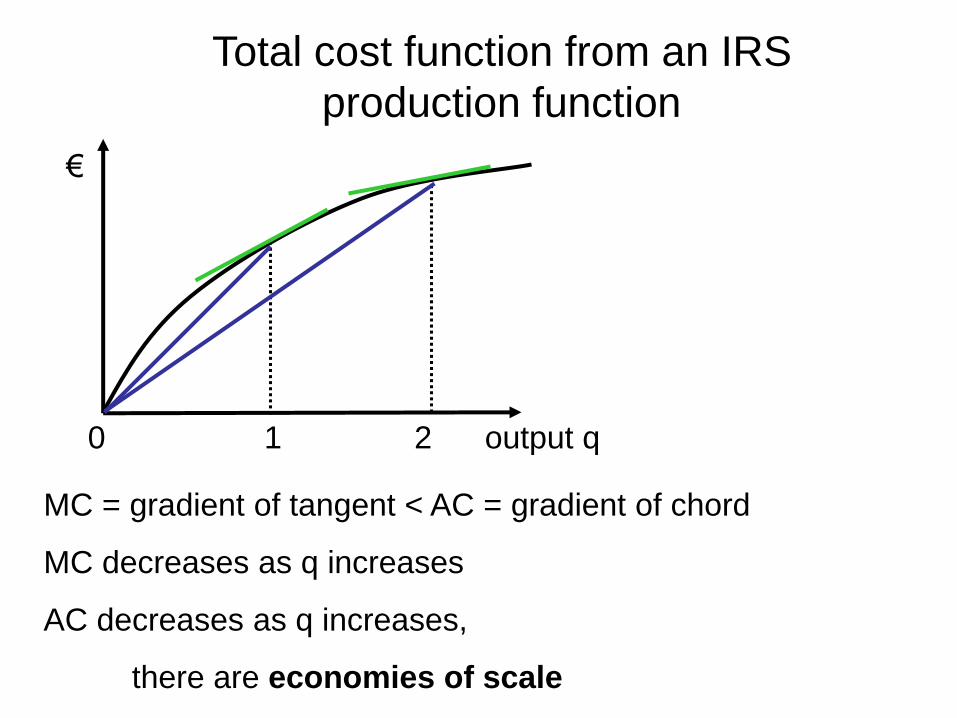
Total cost function from an IRS
production function
AC decreases as q increases,
there are economies of scale
€
0 1 2 output q
Total cost function from an IRS
production function
MC = gradient of tangent < AC = gradient of chord
MC decreases as q increases
AC decreases as q increases,
there are economies of scale

0 output q
€/unit
MC
AC
MC < AC
everywhere
MC ↓ (decreases)
as q ↑
AC ↓ (decreases)
as q ↑
AC and MC from an IRS production function

6. Cost curves and
supply with a u-shaped
average cost curve

6. Cost curves and supply with a u-shaped
average cost curve
• Often assumed for perfect competition.
• For small q and there are economies of scale
AC falls.
• For large q and there are diseconomies of scale
AC rises.

0 a b c output
€
total cost
function
AC falls when
AC rises when
AC has a minimum at
At the minimum AC = MC. The chord is

0 a b c output
€
total cost
function
AC falls when 0 < q < b.
AC rises when
AC has a minimum at
At the minimum AC = MC. The chord is

0 a b c output
€
total cost
function
AC falls when 0 < q < b.
AC rises when b < q.
AC has a minimum at
At the minimum AC = MC. The chord is

0 a b c output
€
total cost
function
AC falls when 0 < q < b.
AC rises when b < q.
AC has a minimum at b.
At the minimum AC = MC. The chord is

0 a b c output
€
total cost
function
AC falls when 0 < q < b.
AC rises when b < q.
AC has a minimum at b.
At the minimum AC = MC. The chord is also a tangent.

0 a b c output
€
total cost
function
MC falls when
MC rises when
MC has a minimum when

0 a b c output
€
total cost
function
MC falls when 0 < q < a.
MC rises when
MC has a minimum when

0 a b c output
€
total cost
function
MC falls when 0 < q < a.
MC rises when a < q.
MC has a minimum when

0 a b c output
€
total cost
function
MC falls when 0 < q < a.
MC rises when a < q.
MC has a minimum when q = a.
0 a b output q
€/unit MC
AC
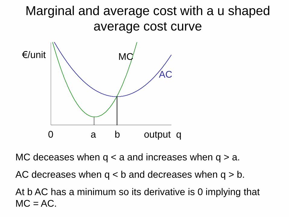
Marginal and average cost with a u shaped
average cost curve
MC deceases when q < a and increases when q > a.
AC decreases when q < b and decreases when q > b.
At b AC has a minimum so its derivative is 0 implying that
MC = AC.

0 a b output q
€/unit MC
AC
min AC
p
Here p < min AC
the firm makes losses at all q > 0,
the shut down condition cannot be satisfied at q > 0 so q = 0.
Profit maximization by a price taking firm with a
u average shaped cost curve
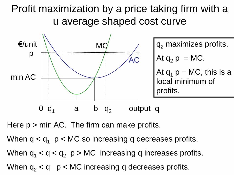
0 q1 a b q2 output q
€/unit MC
AC
Profit maximization by a price taking firm with a
u average shaped cost curve
min AC
p
Here p > min AC. The firm can make profits.
When q < q1 p < MC so increasing q decreases profits.
When q1 < q < q2 p > MC increasing q increases profits.
When q2 < q p < MC increasing q decreases profits.
q2 maximizes profits.
At q2 p = MC.
At q1 p = MC, this is a
local minimum of
profits.

0 q1 a b q2 output q
€/unit MC
AC
Profit maximization by a price taking firm with a
u average shaped cost curve
min AC
p
At q2 p = MC > AC so the firm makes profits > 0. Shutdown &
output conditions are satisfied. q2 maximizes profits
Price = MC at q1 but q1 does not maximize profits.
q1 gives a profit minimum.
0 a b output q
€/unit MC
AC
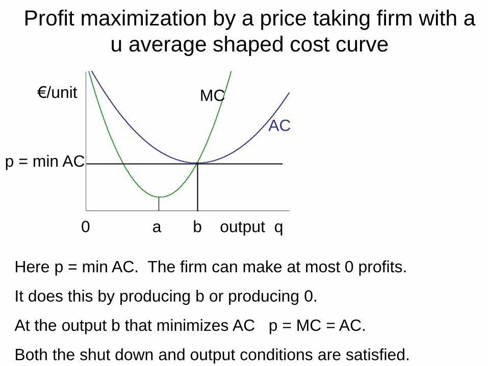
Profit maximization by a price taking firm with a
u average shaped cost curve
p = min AC
Here p = min AC. The firm can make at most 0 profits.
It does this by producing b or producing 0.
At the output b that minimizes AC p = MC = AC.
Both the shut down and output conditions are satisfied.

0 a b output q
p
MCAC
Profit maximization by a price taking firm with a
u average shaped cost curve
When p < min AC the firm produces 0.
When p = min AC the firm produces either 0 or b.
When p > min AC the firm produces on the point where
p = MC, MC is increasing and MC > AC.
supply curve
The supply curve
is the upward
sloping part of the
MC curve where
MC ≥ AC.

7. Long run and short run
costs and supply

7. Long run and short run costs and supply
• Up to now, all inputs are chosen at same time.
• Now there are two periods, the planning period and the
production period.
• Capital is fixed in the planning period and paid for in the
production period.
• Labour is chosen and paid for in the production period.
• If the firm knows output and input prices in the planning
period this makes no difference.
• K and L are chosen to minimize total cost c(v,w,q).

long run
expansion
path
isocost line
gradient – w/v
K
c2/v
c1/v
0 L
q1
isoquant
q2
If in the planning period the firm knows output q and input
prices w & v in the production period it chooses the cost
minimizing point on the long run expansion path.
Total inputs (Li,Ki) total cost LRTC = ci when output is qi.
(L1,K1)
(L2,K2)
ci = LRTC of
output qi
LRTC = long run
total cost

Short Run Costs
• The firm installs K in the planning period, when it is
uncertain what input prices will be and how much it
will produce in the production period.
• The cost s(v,w,K,q) of production depends on input
prices v and w, capital K and output q. It is called
short run total cost (SRTC).
• Contrast LRTC c(v,w,q) does not depend on K.

1. Main: curry or steak
dessert: fruit or cake
2. Main: curry or steak
dessert: fruit
Which menu is better?

Flexibility can never be bad in standard
economics models
• If given the choice between fruit & cake you chose cake
the more restricted menu is worse.
• If given the choice between fruit & cake you chose fruit
the more restricted menu is no better.
• But limiting flexibility may be good if you know you will
eat but regret the cake.
• Limiting flexibility can have advantages in games.

long run
expansion
path
isocost line
gradient – w/v
0 L1 L
q1
isoquant
q2
If in production period K = K1, input prices are w, v and
output is q1 the minimum cost of producing q1 is c1.
K
c2/v
c1/v
K1

0 L’2 L
K
s2/v
c2/v
K1
If in production period K = K1, input prices are w, v and
output is q2 the firm has to use L2’ labour.
Total cost s2/v > c2/v.
c2 = LRTC of
output q2
s2 = SRTC of
output q2
SRTC = short run
total cost
s2 > c2
q1
isoquant
q2

long run
expansion
path
isocost line
gradient – w/v
isoquant
K
K1
0 L
q1
short run
expansion pathq2
q0
With capital fixed at K1 in the planning period the firm is on the
short run expansion path in the production period.
At output q1 the firm is on the long run expansion path.
At other outputs the firm is not on the long run expansion path.
With capital K1
at output q1
LRTC = SRTC.
At other outputs
LRTC < SRTC.

• With a minimization problem you can often do better and
never do worse with more flexibility.
• Long run (choose K and L)
more flexible than
short run (choose L, K fixed).
So either LRTC < SRTC or LRTC = SRTC
LRTC ≤ SRTC always

Long run and short run
costs and supply with a
Cobb-Douglas production
function

Finding SRTC with a Cobb-Douglas
Production Function
Rearrange the production function equation
q = K3/5 L2/5 to get L = q5/2 K-3/2
So to produce q units of output with K = K* requires
q5/2 K*-3/2 units of labour and at prices v and w costs
SRTC = w q5/2 K*-3/2 + vK*.
I have already found that when K and L are chosen
freely
LRTC = [(3/2)2/5 + (2/3)3/5] w2/5 v3/5 q
LRTC depend on v,w,q
SRTC depend on
v,w,K*,q
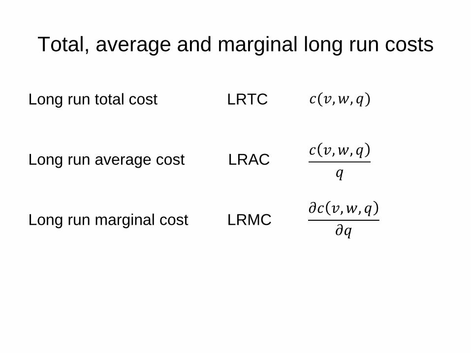
Total, average and marginal long run costs
Long run total cost LRTC
Long run average cost LRAC
Long run marginal cost LRMC

Total, average and marginal short run costs
Short run total cost SRTC
Short run average cost SRAC
Short run marginal cost SRMC

output.on depend costs marginal and averagerun Short
)2/5(
output.on dependnot
do and equal are costs marginal and averagerun long
scale, toreturnsconstant hasfunction production The
])3/2()2/3[(
])3/2()2/3[(
2323
12323
2325
5/35/25/35/2
5/35/25/35/2
5/25/3
/-/
/-/
/-/
K* qwSRMC
vK*q K*w qSRAC
vK* K*w qSRTC
vwLRMCLRAC
qvwLRTC
LKq
so
so
function production Douglas-Cobb the With
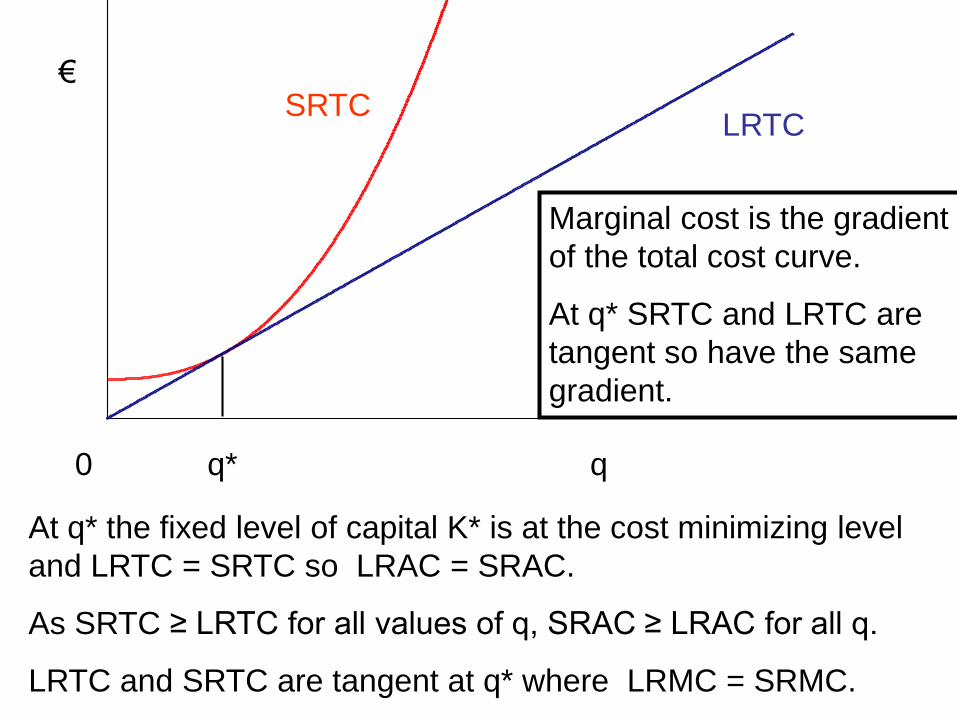
€
0 q* q
SRTCLRTC
At q* the fixed level of capital K* is at the cost minimizing level
and LRTC = SRTC so LRAC = SRAC.
As SRTC ≥ LRTC for all values of q, SRAC ≥ LRAC for all q.
LRTC and SRTC are tangent at q* where LRMC = SRMC.
Marginal cost is the gradient
of the total cost curve.
At q* SRTC and LRTC are
tangent so have the same
gradient.

output.on depend costs marginal and averagerun Short
)2/5(
output.on dependnot
do and equal are costs marginal and averagerun long
scale, toreturnsconstant hasfunction production The
])3/2()2/3[(
])3/2()2/3[(
2323
12323
2325
5/35/25/35/2
5/35/25/35/2
5/25/3
/-/
/-/
/-/
K* qwSRMC
vK*q K*w qSRAC
vK* K*w qSRTC
vwLRMCLRAC
qvwLRTC
LKq
so
so
function production Douglas-Cobb the With

.increasing is so
0)4/15(
respect to with derivative has )2/5(
linestraight horizontal a isgraph so ith not vary w does
v])3/2()2/3[(
2321
2323
3/55/25/35/2
/-/
/-/
K*wq
q K* qwSRMC
q
wLRMCLRAC

12323
12323
2323
12323
2
3
12
5
so
)2/5(
vK*q wK*q
vK*qw K*q
SRACSRMC
K* qwSRMC
vK*q K*w qSRAC
/-/
/-/
/-/
/-/

* when increasing
* when decreasing is so
*3
2 * where*or
*3
2 that implieswhich
2
3ly equivalentor
2
3
if so
5/2
2/525
232512323
qq SRAC
Kw
v qqq
Kw
v q
vK* K*w qvK*qw K*q
SRACSRMC
/
/-//-/
SRAC is u-shaped
with a minimum at q*
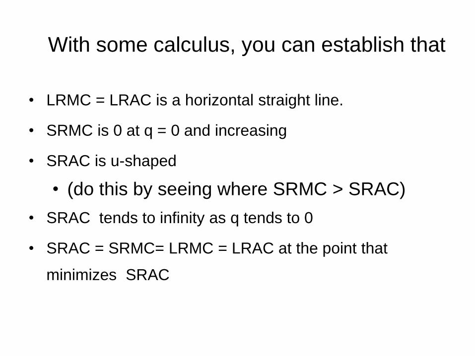
With some calculus, you can establish that
• LRMC = LRAC is a horizontal straight line.
• SRMC is 0 at q = 0 and increasing
• SRAC is u-shaped
• (do this by seeing where SRMC > SRAC)
• SRAC tends to infinity as q tends to 0
• SRAC = SRMC= LRMC = LRAC at the point that
minimizes SRAC

LRAC = LRMC
SRMC
SRAC
0 q* q
LR & SR MC
& AC with this
Cobb-
Douglas
production
function.
At q = q* LRAC = LRMC = SRAC = SRMC
At all values of q SRAC ≥ LRAC
SRMC can be > or < LRMC
€/unit

The General Relationship
Between SR & LR
AC & MC

The General Relationship Between SR & LR
AC & MC
SRAC ≥ LRAC for all q
SRAC = LRAC and SRMC = LRMC at q* where the capital
stock K* would be chosen in the long run.
In the next slides the firm plans for q*.

Perfect competition
Does not imply
LRAC = SRAC = LRMC = SRMC
Why?

The next 2 slides
show a situation in which the capital stock is at the level
that minimizes the long run cost of producing q*,
but q* is not at the level of output that minimizes LRAC.
In this case at q* LRAC = SRAC
& LRMC = SRMC.
But LRAC = SRAC ≠ LRMC = SRMC

0 q* q
€
Here at q* the fixed level of capital K* is at the cost minimizing
level so LRTC = SRTC so LRAC = SRAC.
As SRTC ≥ LRTC for all values of q, SRAC ≥ LRAC for all q.
At q* LRTC and SRTC curves are tangent so the gradient MC is
the same.
LRTC
SRTC
gradient
= SRMC
= LRMC
MC & AC are
different at q*

0 q* q
€
At q* LRAC = SRAC and LRMC = SRMC
But average & marginal costs are different
MC = gradient tangent
AC = gradient chord 0A
LRTC
SRTC
MC & AC are
different at q*
A

The next slide
show a situation in which the capital stock is at the level the
minimizes the long run cost of producing q0
where q0 is the level of output that minimizes LRAC.
In this case only LRAC = SRAC = LRMC = SRMC at q0.
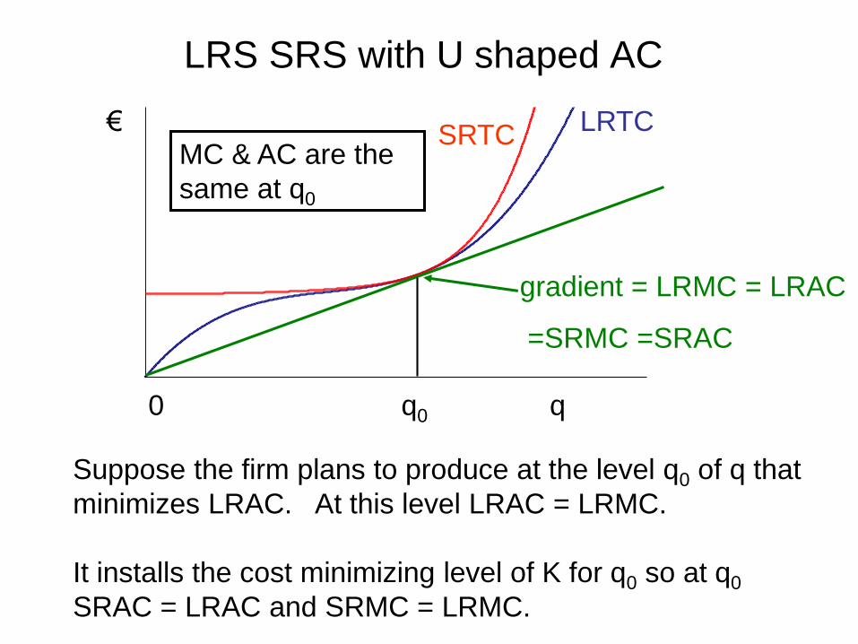
0 q0 q
€SRTC
LRTC
gradient = LRMC = LRAC
=SRMC =SRAC
LRS SRS with U shaped AC
Suppose the firm plans to produce at the level q0 of q that
minimizes LRAC. At this level LRAC = LRMC.
It installs the cost minimizing level of K for q0 so at q0
SRAC = LRAC and SRMC = LRMC.
MC & AC are the
same at q0

Is the short run long run
analysis useful?
What does long run and short run mean?
Economics textbooks:
in the long run all inputs are variable
in the short run some inputs are fixed.
Everyday sense
short run: a temporary state that won’t persist
long run: the state things tend to revert to.
The meanings are similar if the economy tends to come
back to a steady state. Does it?

Is the short run long run analysis useful?
Yes, it captures the idea that unexpected things happen, and if
a firm has to decide on some inputs in advance it may
maximize economic profits by producing even if it makes an
economic loss.
But it is a simple model, and can be very misleading.

What has been achieved
• The implications for supply of profit maximization given
production and cost functions.
• No discussion of the firm as an organization.
• No product differentiation.