Economics Lecture 10vitali/documentsCourses/Lecture...Course Outline 1 Consumer theory and its...
100
Economics Lecture 10 2016-17 Sebastiano Vitali
Transcript of Economics Lecture 10vitali/documentsCourses/Lecture...Course Outline 1 Consumer theory and its...

Economics Lecture 10
2016-17
Sebastiano Vitali

Course Outline
1 Consumer theory and its applications1.1 Preferences and utility
1.2 Utility maximization and uncompensated demand
1.3 Expenditure minimization and compensated demand
1.4 Price changes and welfare
1.5 Labour supply, taxes and benefits
1.6 Saving and borrowing

2 Firms, costs and profit maximization
2.1 Firms and costs
2.2 Profit maximization and costs for a price taking firm
3. Industrial organization
3.1 Perfect competition and monopoly
3.2 Oligopoly and games

3.1 Perfect competition
and monopoly

1. Introduction to industrial organization
2. Markets with a fixed number of price taking firms
3. Firms with different costs & economic rent
4. Welfare economics of a tax with supply and demand
5. Welfare economics of a subsidy with supply and demand
6. Monopoly
7. Cartels
3.1 Perfect competition and monopoly

1. Introduction to industrial organization
One homogeneous good of known quality, no product differentiation
One price for all buyers and sellers
No asymmetric information, buyers know the characteristics of the good and the price charged by each firm.
No transactions costs, e.g.. search, negotiation, legal fees, bid ask spread ….

Market structures
1. perfect competition – price taking firms
2. monopoly – one firm that affects price
3. oligopoly – a small number of firms that affect price
2. Markets with a fixed number of price
taking firms
Perfect competition implies price taking,
nothing a firm does affects the prices it gets for output and
pays for inputs,
nothing a purchaser does affects the price it pays for
output.
See previous lecture
When is price taking plausible?
A homogeneous good, all firms produce an identical product.
Large number of buyers and sellers each with a small market share.
Everyone can observe prices.
Note:
Price taking does not imply that prices do not change.
Price taking does imply that an individual buyer or seller cannot do anything to change prices. See previous lecture

p = MC follows from
Profit maximization implies firms equalize
Profit maximization does not imply that firms produce the level of
See previous lecture
p = MC follows from profit maximization.
Profit maximization implies firms equalize
Profit maximization does not imply that firms produce the level of
See previous lecture
p = MC follows from profit maximization.
Profit maximization implies firms equalize marginal cost of production to price given a surplus per unit of production.
Profit maximization does not imply that firms produce the level of
See previous lecture
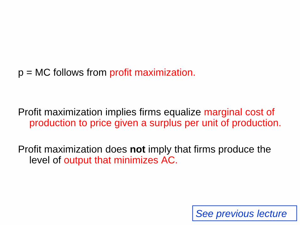
p = MC follows from profit maximization.
Profit maximization implies firms equalize marginal cost of production to price given a surplus per unit of production.
Profit maximization does not imply that firms produce the level of output that minimizes AC.
See previous lecture

Markets with a fixed number
of price taking firms

Markets with price taking firms
Assume for now a fixed set of firms price taking profit maximizing firms.
In an equilibrium with a fixed set of price taking firms
each firm supplies a profit maximizing level of output given input and output prices
The market clears, that is supply = demand.
The next slides show how to solve the model.
Supply and demand are shown as straight lines for simplicity only.
0 q 0 Q
Ss
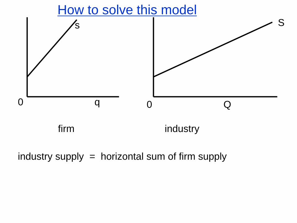
industry supply = horizontal sum of firm supply
How to solve this model
firm industry

0 q 0 Q1 Q
D
Ss
p1
firm industry
industry supply = horizontal sum of firm supply
Find industry price p1 and quantity Q1 by intersection of supply
and demand on industry diagram.
How to solve this model

0 q1 q 0 Q1 Q
D
Ss
p1p1
industry supply = horizontal sum of firm supply
Find industry price p1 and quantity Q1 by intersection of supply
and demand on industry diagram.
Given the industry price find firm output q1 on firm diagram.
How to solve this model
firm industry

0 q1 q 0 Q1 Q2
Ss
p1
D1
Increase in demand
D2p1
Demand curve shifts ( demand at each price)
Industry diagram price from p1 to , Q from Q1 to .
Firm diagram firm quantity from q1 to .

0 q1 q 0 Q1 Q2
Ss
p1
D1
Increase in demand
D2p1
Demand curve shifts ( demand at each price)
Industry diagram price from p1 to , Q from Q1 to .
Firm diagram firm quantity from q1 to .

0 q1 q 0 Q1
Ss
p1
D1
Increase in demand
D2p1
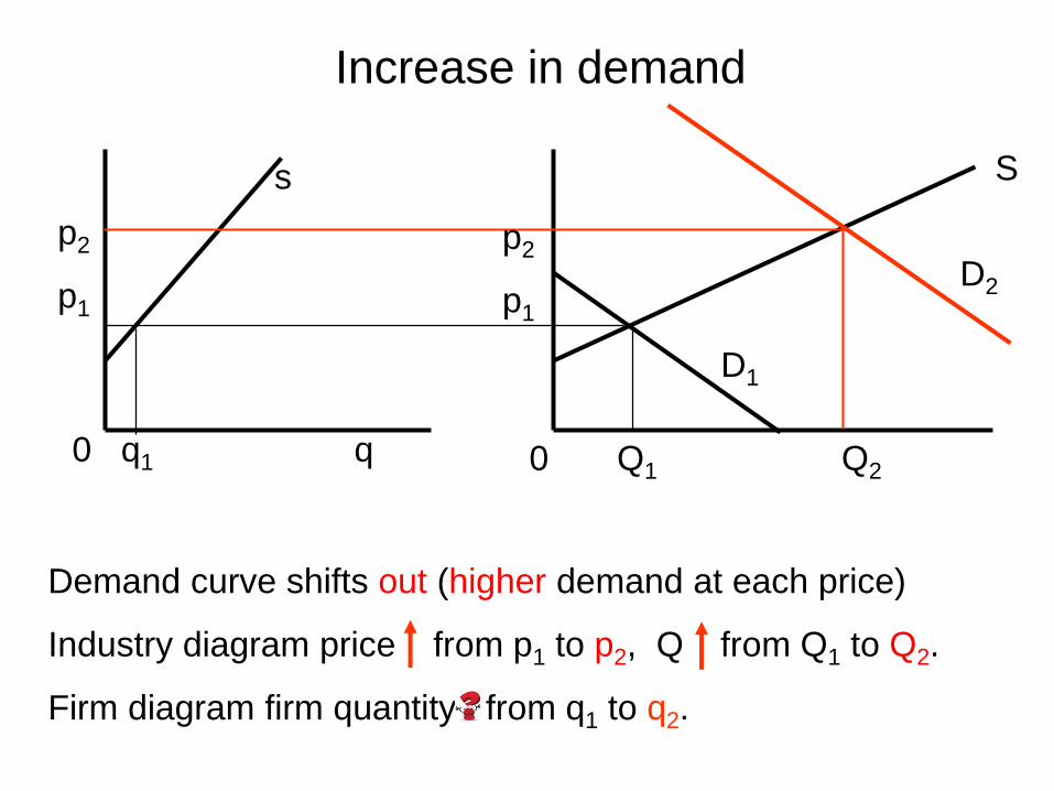
Demand curve shifts out (higher demand at each price)
Industry diagram price from p1 to p2, Q from Q1 to Q2.
Firm diagram firm quantity from q1 to .
0 q1 q 0 Q1 Q2
Ss
p2
p1
D1
Increase in demand
D2
p2
p1
Demand curve shifts out (higher demand at each price)
Industry diagram price ↑ from p1 to p2, Q ↑ from Q1 to Q2.
Firm diagram firm quantity from q1 to q2.

0 q1 q2 q 0 Q1 Q2
Ss
p2
p1
D1
Increase in demand
D2
p2
p1
Demand curve shifts out (higher demand at each price)
Industry diagram price ↑ from p1 to p2, Q ↑ from Q1 to Q2.
Firm diagram firm quantity from q1 to q2.

0 q1 q 0 Q1 Q
D
S1
s1
firm industry
p1
Change in marginal cost
Increase in input prices MC.
Supply curves s1 & S1 move
Industry diagram price from p1 to , Q from Q1 to .
Firm diagram firm quantity from q1 to .
p1

0 q1 q 0 Q1 Q
D
S1
s1
firm industry
p1
Increase in input prices MC.
Supply curves s1 & S1 move to s2 & S2.
Industry diagram price from p1 to , Q from Q1 to .
Firm diagram firm quantity from q1 to .
p1
Change in marginal cost

Change in marginal cost
0 q1 q 0 Q1 Q
D
S1
s1
firm industry
p1
s2
S2
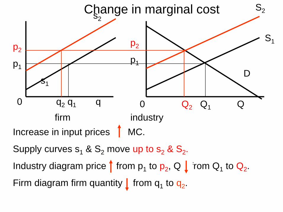
Increase in input prices ↑ MC.
Supply curves s1 & S1 move up to s2 & S2.
Industry diagram price from p1 to p2, Q from Q1 to Q2.
Firm diagram firm quantity from q1 to .
p1

0 q1 q 0 Q2 Q1 Q
D
S1
s1
firm industry
p2
p1
s2
S2
Increase in input prices ↑ MC.
Supply curves s1 & S2 move up to s2 & S2.
Industry diagram price ↑ from p1 to p2, Q ↓ from Q1 to Q2.
Firm diagram firm quantity from q1 to q2.
p2
p1
Change in marginal cost
0 q2 q1 q 0 Q2 Q1 Q
D
S1
s1
firm industry
p2
p1
s2
S2
Increase in input prices ↑ MC.
Supply curves s1 & S2 move up to s2 & S2.
Industry diagram price ↑ from p1 to p2, Q ↓ from Q1 to Q2.
Firm diagram firm quantity from q1 to q2.
p2
p1
Change in marginal cost

q
c
0
Usually AC & MC depend on q and input
prices.
With constant returns to scale AC = MC and
does not vary with q. AC & MC do depend on
input prices.
MC = AC = c
When p = c the firm makes the same profits
(0) at any q. The firm’s output is not
determined.
Special
Case
CRS
the firm’s
supply
See previous lecture

q Q
industry supply = horizontal sum of firms’ supply
industry quantity Q comes from intersection supply and demand
on the industry diagram.
Price = c. Firm supply is not determined.
Equilibrium in a market with a fixed set of price
taking firms and CRS
c c
firm industry
demand
industry
supply

Firms with different costs
& economic rent

Up to now:
models in which all firms have including potential
entrants have the same costs.
Different firms may have different costs, due to different
technologies or access to different quality inputs.
I will look at the effects of access to different quality inputs.
3. Firms with different costs & economic rent

Case 1: Entry Costs
There is a cost to entering the industry. For firms already
in the industry this is a sunk cost and not an opportunity
cost.
For potential entrants this is an opportunity cost.
If at the industry price
0 < profits for firms in the industry < entry costs
firms in the industry make positive profits in entry and exit
equilibrium.

Case 2: some firms have higher quality
inputs which can’t be traded
Some inputs come in different qualities.
If either the difference can’t be observed so high and low
quality inputs trade at the same price
or it is not possible to trade the inputs
firms with higher quality inputs have lower costs and higher
profits.

Case 3: some firms have higher quality
inputs which can be traded.
Some inputs come in different qualities.
Now suppose these inputs can be traded.
Higher quality inputs have higher prices.
In the simplest case all the extra profits that firms have with
high quality inputs that can’t be traded go into the price of
these inputs.
Now firms with high quality inputs make 0 profits.

Economic Rent
Originally this story about different quality inputs was
about farming with varying land quality.
With no market for land farmers with high quality land
make economic profits.
With a market for land all the profits go to the landowner in
the form of rent.
Farmers that do not own the land make 0 profits.
Rent is sometimes used as a term for profits.

A very simple model of rent in a price
taking oil industry
• There are two types of input.
• “High quality” onshore wells, MC = AC = c1,
total capacity Q1.
• “Low quality” offshore wells, MC = AC = c2 > c1,
total capacity Q2.

0 Q1 Q2
€
c2
c1
€
c2
c1
0 Q1 Q1 + Q2
Onshore
supply
Offshore
supply Industry supply
add supply curves horizontally

€
c2
c1
0 Q Q1 Q1 + Q2
Supply = demand at Q where 0 < Q < Q1. Then p = c1.
Onshore wells make 0 profits & produce less than maximum Q1.
Offshore wells do not produce and make 0 profits.
Industry supply & demand with different demand curves
Solve for S =D
accurate diagram
or find Q at p = c1 & p = c2
then use a diagram
DS
€
c2
c1
0 Q1 Q1 + Q2
Industry supply & demand with different demand curves
D S
pSolve for S =D
accurate diagram
or find Q at p = c1 & p = c2
then use a diagram
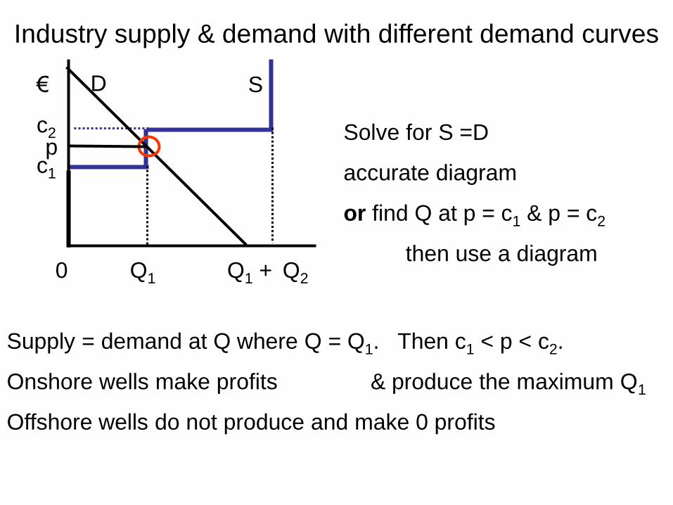
Supply = demand at Q where Q = Q1. Then c1 < p < c2.
Onshore wells make profits & produce the maximum Q1
Offshore wells do not produce and make 0 profits

€
c2
c1
0 Q1 Q1 + Q2
Industry supply & demand with different demand curves
D S
pSolve for S =D
accurate diagram
or find Q at p = c1 & p = c2
then use a diagram
Supply = demand at Q where Q = Q1. Then c1 < p < c2.
Onshore wells make profits & produce the maximum Q1
Offshore wells do not produce and make 0 profits

€
c2
c1
0 Q1Q Q1 + Q2
Industry supply & demand with different demand curves
D S
Supply = demand at Q where Q1 < Q < Q1 + Q2. p = c2.
Onshore wells make profits & produce the maximum Q1
Offshore wells produce < Q2 & make 0 profits

€
c2
c1
0 Q1Q Q1 + Q2
Industry supply & demand with different demand curves
D S
Supply = demand at Q where Q1 < Q < Q1 + Q2. p = c2.
Onshore wells make profits & produce the maximum Q1
Offshore wells produce < Q2 & make 0 profits

€
p
c2
c1
0 Q1 Q1 + Q2
Industry supply & demand with different demand curves
D
S
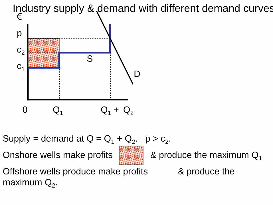
Supply = demand at Q = Q1 + Q2. p > c2.
Onshore wells make profits & produce the maximum Q1
Offshore wells produce make profits & produce the
maximum Q2.
€
p
c2
c1
0 Q1 Q1 + Q2
Industry supply & demand with different demand curves
D
S
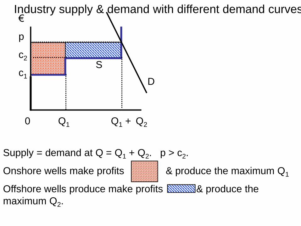
Supply = demand at Q = Q1 + Q2. p > c2.
Onshore wells make profits & produce the maximum Q1
Offshore wells produce make profits & produce the
maximum Q2.
€
p
c2
c1
0 Q1 Q1 + Q2
Industry supply & demand with different demand curves
D
S
Supply = demand at Q = Q1 + Q2. p > c2.
Onshore wells make profits & produce the maximum Q1
Offshore wells produce make profits & produce the
maximum Q2.

Welfare economics of a
tax with supply and
demand

4. Welfare economics of a tax with supply
and demandAssume that firms’ costs = social costs
A strong assumption requiring no externalities and perfectly competitive input markets
This assumes that distribution is not an issue, the social gain of giving €1 to someone does not depend on wealth, income ….

Total cost = F + v(q)
= fixed cost + variable cost.
v'(q) = derivative of variable cost
= MC.
Integration, v(q1) is area under MC
curve.0 q1 q
MC = v'(q)p1
Total revenue = p1q1 =
Producer surplus = total revenue – variable cost
If there is no fixed cost producer surplus = profit.
Producer surplus for a firm
v(q1)
PS

0 q1 q 0 Q1 Q
D
Ss
p1p1
industry consumer surplus
sum the firm’s supply curve horizontally to get industry supply
and industry producer surplus
firm industry
Industry consumer and producer surplus

Assume for simplicity the tax t is per unit sold, not % of
price
Example excise tax on cigarettes, alcohol, petrol.
The tax t per unit increases marginal cost by t
Welfare economics with supply and demand
example 1 tax

Effects of a tax in an industry with CRS
If the tax is t and price paid by consumers is p
firms get p – t.
If all firms have CRS so constant AC & MC c
profits from supplying q are (p – t – c)q
profits are 0 when p = c + t,
supply with tax is perfectly elastic at c + t
Assuming that input prices don’t change when the industry
expands industry supply with the tax is horizontal at c + t.

q Q2 Q1 Q
with no tax price is c (= AC = MC), industry produces Q1
with the tax price is c + t, industry produces Q2,
tax revenue = tQ2
Effect of an excise tax in an industry with CRS
p = c + t
c
firm industry
demand
p
c
s with tax
s no tax
S with tax
S no tax
D

price p
supply
Q2 Q1 Q
c + t
c
Effects of an excise tax with CRS
demand
With CRS there is no producer surplus.
With no tax price = c, industry output Q1
Consumer surplus = entire shaded area.
With tax t price = c + t, Q falls to Q2, tax revenue =
loss consumer surplus = > tax revenue
Firms make
0 profits with
and without
tax.

Definition of deadweight loss due to tax
deadweight loss =
loss of producer & consumer surplus – tax revenue
In this case loss of producer surplus = 0
loss of consumer surplus ≈ equivalent variation
deadweight loss ≈ equivalent variation – tax revenue
= excess burden of the tax to the consumer

price p
demand
supply
Q2 Q1 Q
c + t
c
Here demand is more elastic,
deadweight loss area = ½ t (Q1 – Q2)
is a larger fraction of tax revenue area = t Q2
Effects of an excise tax with CRS
))((2
1
2
1
2
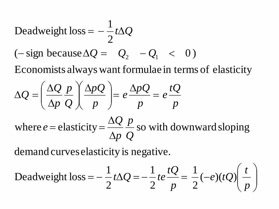
1 loss Deadweight
negative. is elasticity curves demand
sloping downward with so elasticity where
elasticity of in terms formulae want always Economists
) 0 becausesign (
2
1 loss Deadweight
12
p
ttQe
p
tQteQt
Q
p
p
Qe
p
tQe
p
pQe
p
pQ
Q
p
p
QQQ
Qt

pricein increase ateproportionelasticity -2
1
revenuetax
loss deadweight
pricein increase ateproportion /
revenue, tax
))((2
1
2
1 loss Deadweight
pt
tQ
p
ttQe
p
tQte
Implication
Given target tax revenue it is better to raise tax revenue
by taxing goods whose demand is inelastic.
But this ignores distribution.
If the good is a large proportion of the consumption of
poor people and you want to take this into account this
argument is too simple.
The analysis can be extended to take explicit account of
distributional value judgements, but has to be done with
maths not diagrams.
Not in this course.
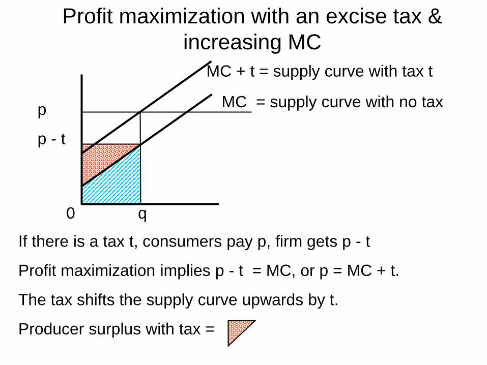
If there is a tax t, consumers pay p, firm gets p - t
Profit maximization implies p - t = MC, or p = MC + t.
The tax shifts the supply curve upwards by t.
Producer surplus with tax =
0 q
Profit maximization with an excise tax &
increasing MC
MC = supply curve with no tax
MC + t = supply curve with tax t
p
p - t

0 q2 q1 q 0 Q2 Q1 Q
D
S no tax
with no tax price p1, industry Q1, firm q1
With tax price p2 industry Q2 at intersection D and S with tax.
consumer surplus = producer surplus =
tax revenue tQ2 =
firm industry
Supply and demand with tax
p2
p1
p2 - t
S with tax
tt

0 Q2 Q1 Q
D
S no taxp2
p1
p2 - t
S with tax
tindustry
diagram
tax revenue
deadweight loss = loss of surplus – tax revenue
Any form of tax except lump sum taxes involves a
deadweight loss.
Politically acceptable lump sum taxes are not feasible.
loss of consumer surplus
loss of producer surplus

p
p2
p1
p2 - t
Q2 Q1 Q
supply with tax
supply with no tax
Ddemand more elastic
than supply
loss PS > loss CS
Price paid by consumer
increases much less
than tax.

p
p2
p1
p2 - t
Q2 Q1 Q
supply with tax
supply with no tax
D
demand less elastic
than supply
loss PS < loss CS

Q2 Q1 Q
p
p2
p1
p2 - t
D
S no tax
S with tax
supply and
demand are
elastic,
deadweight loss
is a large fraction
of tax revenue

Q2 Q1 Q
p
p2
p1
p2 - t
D
S no tax
S with tax
supply and
demand are
inelastic,
deadweight loss
is a small fraction
of tax revenue

Welfare economics of a
subsidy with supply and
demand

Assume for simplicity the subsidy s is per unit sold, not
% of price,
subsidies are particularly common on food, housing
and agricultural products.
With a subsidy s consumers pay p , producers get
p + s so supply at the point where MC = p + s or
p = MC - s
5. Welfare economics of a subsidy with
supply and demand

0 q
Supply by a firm with a subsidy
MC - s = supply curve with
subsidy
MC = supply curve no subsidy
p + s
p
If there is a subsidy s & consumers pay p the firm gets p + s
on each unit.
Profit maximization implies p + s = MC, or p = MC - s.
The subsidy shifts the supply curve downwards by s.
Producer surplus with subsidy =

demand from
consumers
Q1 Q2 Q
price
p2 + s
p1
p2
With no subsidy Q = Q1 p = p1,
with subsidy price consumers pay falls to p2
price producers get rises to p2 + s
Q expands to Q2
supply no
subsidy
supply with
subsidy
Supply &
demand
with a
subsidy
s

demand from
consumers
Q1 Q2 Q
price
p2 + s
p1
p2
gain in producer surplus
gain in consumer surplus
entire shaded area = cost of subsidy = sQ2
deadweight loss = cost of subsidy
– gain from subsidy
supply with
subsidy
simple
welfare
economics
of a subsidy
s

demand
Q1Q2 Q
price
p2 + s
gain in producer surplus
gain in consumer surplus
entire shaded area = cost of subsidy = sQ2
deadweight loss = cost of subsidy
– loss of surplus
simple
welfare
economics
of a subsidy
s
p1
p2
With less elastic
supply most of the
gain in surplus
goes to producers

demand
Q1 Q
price
p1 + s
gain in producer surplussimple
welfare
economics
of a subsidy
p1
With completely
inelastic supply all
the gain in surplus
goes to producers.
There is no
increase in quantity
or consumer
surplus. There is
no deadweight loss
The gain in consumer and producer surplus from a subsidy is
less than the cost of the subsidy.
Who gains from the subsidy on some agricultural products from
the Common Agricultural Policy of the European Union?
Simple argument: the cost of subsidy exceeds the benefit to
farmers and consumers.
Effects on farmers outside the EU are also important.
The subsidies increases the value of agricultural land.
Land owners gain when the subsidy is introduced, and would
lose if the subsidy were removed.

With supply and demand analysis
Remember the limits of supply and demand analysis
Any policy that puts a gap between what consumers pay
and producers get moves quantity from the level that
maximizes surplus.
assumes price taking.
Consumers know the prices and quality, no asymmetric
information
Input prices reflect social costs, so no externalities,
perfect competition in the input markets.
Distribution is not taken into account.

Monopoly

6. Monopoly
Up to now I have assumed that firms are price takers.
They are small relative to the market so their output decisions
have no effect on prices.
Now look at industries with one firm (monopoly)
Later look at industries with a small number of firms (oligopoly).

Why are there industries with a small
number of firms?
• Economies of scale
– to be discussed later.
• Legal barriers to entry
– e.g. licenses, quotas, state monopolies
• Access to a critical input or technology that is not available to other firms,
– patents
– secrecy making imitation impossible
– organizational culture

If q > 0 maximizes profits the first order conditions imply
Π’(q) = R’(q) – c'(q) = 0 or
MR marginal revenue = R’(q) = c'(q) = marginal cost.
This is the marginal output rule.
If c(0) = 0 then if q = 0 profits = 0.
Profit maximization then implies Π(q) = R(q) – c(q) ≥ 0
so if q > 0 maximizes profits
average revenue = R(q)/q = p ≥ c(q)/q = AC
That is p ≥ AC, the shutdown rule.
price ) 1
1( revenue marginal so
) 1
1(
) 1(
pe
pMR
e
p
q
q
pe
ep
q
p
p
qp
q
p q p
q
pqqp
q
R MR
sloping downward is demand because 0
demand. of elasticity price own where
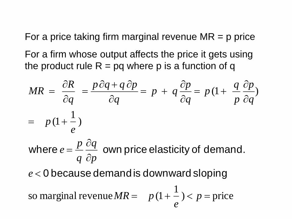
For a price taking firm marginal revenue MR = p price
For a firm whose output affects the price it gets using
the product rule R = pq where p is a function of q

Profit maximization implies MC = MR < p so MC < p
For a monopoly elasticity, MR and output depend only on
demand from buyers.
For a firm in a oligopoly elasticity, MR and output depend
on demand from buyers and the output by other firms in
the industry.

Exam mistake with perfect competition
models
• Working with perfect competition model
• Finding industry revenue
• Finding industry marginal revenue
• Equating industry marginal revenue to marginal cost.
• In perfect competition there is price taking
• Firm marginal revenue = price
• Find firm supply as a function of price
• Equate total supply by all firms to demand
WRONG
RIGHT

Throughout this section
Q = industry supply = demand when = Q = - p
where p = price so p(Q) = a – bQ
where a = / and b = 1/
Assume that > 0 & > 0 so a > 0 and b > 0.
For a monopoly total revenue p(Q)Q = (a – bQ)Q = aQ –
bQ2.
Marginal revenue =
derivative of total revenue with respect to Q = a – 2bQ.
A simple model of demand

Example monopoly with constant returns to
scale (CRS)the algebra
A firm is a monopoly when there is no other firm producing
the same good.
With CRS the firm’s total cost is cQ where c = MC = AC.
If price = a – bQ profits p(Q)Q – cQ = (p(Q) – c)Q
= (a – bQ – c) Q = (a – c)Q – bQ2.
If a c profits are negative for all Q > 0, the firm produces 0.

If a > c profits (a – c)Q – bQ2 are a quadratic in Q with a
negative coefficient of Q2 .
The foc (first order conditions) give a maximum where the
derivative is 0, that is a – c – 2bQ = 0 .
The same condition can be got from
MR = marginal revenue = marginal cost = c.
Total revenue = p(Q)Q = (a – bQ)Q = a – bQ2
differentiating with respect to Q gives MR = a – 2bQ
so MR = MC gives a – 2bQ = c
or a – c – 2bQ = 0.
Many people
don’t say this in
the exam.

From the first order condition MR = MC
a – c – 2bQ = 0 so profits are maximized when
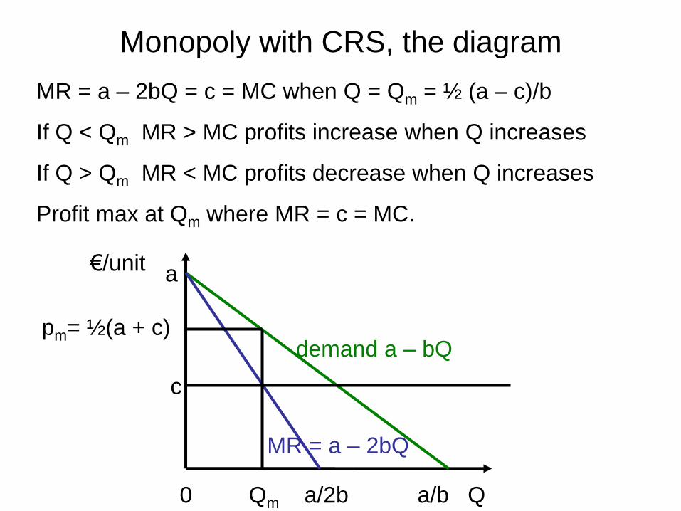
Q = Qm = ½ (a – c)/b.
price pm = a – b Qm = a - ½ (a – c) = ½ a + ½ c > c because
a > c.
profits = total revenue – total cost = pmQm – cQm
= (pm – c)Qm = ½ (a – c)Qm = ¼ (a – c)2 /b.
c
a
pm= ½(a + c) demand a – bQ
0 Qm a/2b a/b Q
MR = a – 2bQ
€/unit
MR = a – 2bQ = c = MC when Q = Qm = ½ (a – c)/b
If Q < Qm MR > MC profits increase when Q increases
If Q > Qm MR < MC profits decrease when Q increases
Profit max at Qm where MR = c = MC.
Monopoly with CRS, the diagram

Demand gives p(Q) = a – bQ, profits = total revenue – total cost
= p(Q)Q – cQ – F = (a – bQ)Q – cQ - F = (a - c)Q – bQ2 - F
If a c profits < 0 for all Q > 0 the firm does not produce.
If a > c profits are a quadratic function of Q with a negative
coefficient on Q2.
Monopoly with the cost function c(q) = F + cq

If Q > 0 and profits are maximized the foc is a – c – 2bQ = 0
so Q = ½ (a – c)/b > 0
Price p(Q) = a – bQ = a - ½ (a – c) = ½ (a + c) = c + ½ (a – c) > c
Profits = p(Q) - c(Q) = (p(Q) – c)Q – F = (a – c)2 /(4b) - F.
If F > (a – c)2 /(4b) the firm cannot make a profit so shuts down.
Monopoly with the cost function c(Q) = F + cQ

AC = c + F/q
MC = c
€/unit
a
pm
0 Qm a/2b a/b Q
c
Case 1 (a – c)2 /(4b) - F 0
At Qm = ½ (a – c)/b MR = MC and
price pm = ½ a + ½ c > c + F/q = AC.
Price and quantity are the same as
in the CRS case but profits are
(a – c)2 /(4b) - F 0.
MR
demand

AC = c + F/q
MC = c
€/unit
a
pa
0 Qa a/2b a/b Q
c
Case 2 (a – c)2 /(4b) - F < 0
At Qa MR = MC and profits are
higher than at any other Q > 0
But price pa < c + F/q = AC.
The monopoly makes losses at all
Q > 0 so does not produce.
€/unit
pm
c
0 Qm QC Q
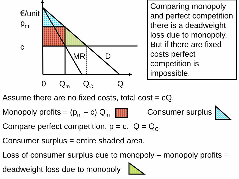
Assume there are no fixed costs, total cost = cQ.
Monopoly profits = (pm – c) Qm Consumer surplus
Compare perfect competition, p = c, Q = QC
Consumer surplus = entire shaded area.
Loss of consumer surplus due to monopoly – monopoly profits =
deadweight loss due to monopoly
DMR
Comparing monopoly
and perfect competition
there is a deadweight
loss due to monopoly.
But if there are fixed
costs perfect
competition is
impossible.

Cartels

7. Cartels
Suppose that there are n firms in an industry that have a cartelagreement to maximize industry profits.
Suppose firm i has costs cqi + F.
Assume F > 0 so there are economies of scale.
Total industry cost
= c(q1 + q2 …..qn) + nF = cQ + nF where Q = q1 + q2 …..qn.
Assume as before p = a – bQ.
Industry profits pQ – c Q – nF = (a – bQ - c)Q – nF
Same as monopoly profits except last term is nF not F.

Cartels
Industry profits = (a – bQ - c)Q – nF
= (a – c) Q – bQ2 – nF.
If a c the industry cannot make profits.
If a > c and the industry produces Q > 0
the formula for profits is the same as with monopoly except the
fixed cost is nF not F.

Cartels
If Q > 0 maximizes profits Q = ½ (a – c) /b
price p = ½ (a + c),
p and Q are the same as with a monopoly but
cartel profits (a – c)2 /(4b) - nF
< monopoly profits (a – c)2 /(4b) - F.

If n > (a – c)2 /(4bF) the cartel makes losses,
so at least one firm in the industry makes losses.
As the cartel maximizes industry profits if n > (a – c)2 /(4bF)
there is no way the industry can be profitable at any level of
output.
An industry with n > (a – c)2 /(4bF) is impossible when there is
entry and exit.

A large fixed cost F is a barrier to entry
as is low demand, small a or large b.
If F < (a – c)2 /(4b) < 2F a monopoly can make profits but
if there are 2 or more firms the industry makes losses.
The industry must be a monopoly.

What have we achieved?
• Simple model of perfect competition,
• with limitations but useful policy insights.
• Simple models of monopoly & cartels
• major limitation: very little discussion of innovation.