ECONOMIC SUPPLY & DEMAND - The Creative...

D-4388-2 08/12/03 1

ECONOMIC SUPPLY & DEMAND

by

Joseph Whelan

Kamil Msefer

Vemsim Examples added by Nathaniel Choge

February 2001

Prepared for the

MIT System Dynamics in Education Project

Under the Supervision of

Professor Jay W. Forrester

August 12, 2003

Copyright ©2001 by MIT

Permission granted to copy for non-commercial educational purposes

11:24 PM 08/12/03 D-4388-22

D-4388-2 08/12/03 3

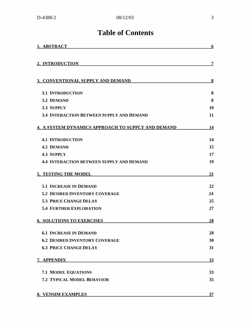
Table of Contents

1. ABSTRACT 6

2. INTRODUCTION 7

3. CONVENTIONAL SUPPLY AND DEMAND 8

3.1 INTRODUCTION 8

3.2 DEMAND 8

3.3 SUPPLY 10

3.4 INTERACTION BETWEEN SUPPLY AND DEMAND 11

4. A SYSTEM DYNAMICS APPROACH TO SUPPLY AND DEMAND 14

4.1 INTRODUCTION 14

4.2 DEMAND 15

4.3 SUPPLY 17

4.4 INTERACTION BETWEEN SUPPLY AND DEMAND 19

5. TESTING THE MODEL 21

5.1 INCREASE IN DEMAND 22

5.2 DESIRED INVENTORY COVERAGE 24

5.3 PRICE CHANGE DELAY 25

5.4 FURTHER EXPLORATION 27

6. SOLUTIONS TO EXERCISES 28

6.1 INCREASE IN DEMAND 28

6.2 DESIRED INVENTORY COVERAGE 30

6.3 PRICE CHANGE DELAY 31

7. APPENDIX 33

7.1 MODEL EQUATIONS 33

7.2 TYPICAL MODEL BEHAVIOR 35

8. VENSIM EXAMPLES 37

11:24 PM 08/12/03 D-4388-24

D-4388-2 08/12/03 5

1. ABSTRACT

The main purpose of this paper is to discuss supply and demand in the framework

of system dynamics. We first review classical supply and demand. Then we look at how

to model supply and demand using system dynamics. Finally, we present a few exercises

that will improve understanding of supply and demand and help improve system

dynamics modeling skills.

11:24 PM 08/12/03 D-4388-26

2. INTRODUCTION

This paper emerged as an attempt to use system dynamics to model supply1 and

demand. Classical economics presents a relatively static model of the interactions among

price, supply and demand. The supply and demand curves which are used in most

economics textbooks show the dependence of supply and demand on price, but do not

provide adequate information on how equilibrium is reached, or the time scale involved.

Classical economics has been unable to simplify the explanation of the dynamics

involved. Additionally, the effects of excess or inadequate inventory are often not

discussed.

In the real world, the market price is affected by the inventory of goods held by

the manufacturers rather than the rate at which manufacturers are supplying goods.2 If

the manufacturers are supplying goods at a rate equal to the consumer demand, the static

classical theory would propose that the market is in equilibrium. However, what if there

is a tremendous surplus in the store supply rooms? The manufacturers will lower the

price and/or decrease production to return inventory to a desired level.

This paper introduces a model that incorporates elements from classical

economics as well as several real-world assumptions. This model will be used to

examine some of the interactions among supply, demand and price.

1 Supply and production are very similar terms and are often used interchangeably.

2Low, Gilbert W. (1974). Supply and Demand in a Single-Product Market (Exercise Prepared for the

Economics Workshop of the System Dynamics Conference at Dartmouth College, Summer 1974)

(Department Memorandum No. D-2058). M.I.T., System Dynamics Group.

D-4388-2 08/12/03 7

3. CONVENTIONAL SUPPLY AND DEMAND

3.1 Introduction

This section deals with supply and demand as sometimes taught in high-school

economics classes. The following descriptions of supply and demand assume a perfectly

competitive market, rational consumers, and free entry and exit into the market.

Economists also make the simplification that all factors other than price which affect the

quantity of goods sold and purchased are held constant. Economists argue that this is a

valid assumption because changes in price occur much more quickly than changes in

other factors that may affect supply or demand. Examples of these other factors include

changes in taste, changes in the state of the economy and long-term changes in

production capacity (such as the construction of a new factory).

3.2 Demand

Demand is the rate at which consumers want to buy a product. Economic theory

holds that demand consists of two factors: taste and ability to buy. Taste, which is the

desire for a good, determines the willingness to buy the good at a specific price. Ability

to buy means that to buy a good at specific price, an individual must possess sufficient

wealth or income.

Both factors of demand depend on the market price. When the market price for a

product is high, the demand will be low. When price is low, demand is high. At very

low prices, many consumers will be able to purchase a product. However, people usually

want only so much of a good. Acquiring additional increments of a good or service in

some time period will yield less and less satisfaction.3 As a result, the demand for a

product at low prices is limited by taste and is not infinite even when the price equals

zero. As the price increases, the same amount of money will purchase fewer products.

When the price for a product is very high, the demand will decrease because, while

consumers may wish to purchase a product very much, they are limited by their ability to

buy.

The curve in Figure 1 shows a generalized relationship between the price of a

good and the quantity which consumers are willing to purchase in a given time period.

This is known as a simple demand curve.

3 This behavior toward aquiring additional increments of a good is called diminishing marginal utility.

11:24 PM 08/12/03 D-4388-28

Demand Limited by ability to buy

Demand Limited by taste

Pric

e

Rate of PurchaseFigure 1: Demand Curve4

This curve shows the rate at which consumers wish to purchase a product at a givenprice.

The simple demand curve seems to imply that price is the only factor which

affects demand. Naturally, this is not the case. Recall the assumption made by

economists that the other factors which influence changes in demand act over a much

larger time frame. These factors are assumed to be constant over the time period in

which price causes supply and demand to stabilize.

4 The reader should note that the convention in economic theory is to plot the price on the vertical axis and

the rate of purchase on the horizontal axis.

D-4388-2 08/12/03 9

3.3 Supply

Willingness and ability to supply goods determine the seller’s actions. At higher

prices, more of the commodity will be available to the buyers. This is because the

suppliers will be able to maintain a profit despite the higher costs of production that may

result from short-term expansion of their capacity5.

In a real market, when the inventory is less than the desired inventory,

manufacturers will raise both the supply of their product and its price. The short-term

increase in supply causes manufacturing costs to rise, leading to a further increase in

price. The price change in turn increases the desired rate of production. A similar effect

occurs if inventory is too high. Classical economic theory has approximated this

complicated process through the supply curve. The supply curve shown in Figure 2

slopes upward because each additional unit is assumed to be more difficult or expensive

to make than the previous one, and therefore requires a higher price to justify its

production.

Supply

Pric

e

Figure 2: Supply CurveAt high prices, there is more incentive to increase production of a good. This graphrepresents the short-term approximation of classical economic theory.

5Short-term expansion can be achieved by giving workers overtime hours, contracting to an outside source,

or increasing the load on current equipment. These types of changes increase per-unit supply costs.

11:24 PM 08/12/03 D-4388-210

3.4 Interaction Between Supply and Demand

Demand is defined as the quantity (or amount) of a good or service people are

willing and able to buy at different prices, while supply is defined as how much of a good

or service is offered at each price. How do they interact to control the market?

Buyers and sellers react in opposite ways to a change in price. When price

increases, the willingness and ability of sellers to offer goods will increase, while the

willingness and ability of buyers to purchase goods will decrease. To illustrate more

clearly how the market works, we will look at the following example from the clothing

industry.

Table 1 is called a schedule of demand and supply. For each price, it indicates

how much clothing is demanded by the consumers per week, and how much clothing is

supplied per week. Notice that as price decreases, demand increases and supply

decreases. Eventually demand exceeds supply.

D-4388-2 08/12/03 11

Demand and Supply SchedulesPrice Quantity Quantity

Demanded Supplied(per week) (per week)

---------------------------------------------------------------

$50 10 100

$45 14 97

$40 18 94

$35 22 89

$30 28 84

$25 35 77

$20 45 68

$15 57 57

$10 73 40

$5 100 0

Table 1: Demand and Supply SchedulesFor each price, the schedule above indicates the quantity (in articles per week) of clothingdemanded and supplied.

The market will reach equilibrium when the quantity demanded and the quantity

supplied are equal. At $15, supply and demand are equal at 57 articles of clothing per

week. To better understand the dynamics involved, suppose that one article of clothing

was selling for $30. Producers would be willing to supply 84 articles of clothing per

week, but consumers would only be buying 28 articles per week. As a result, the

producers would have excess inventory piling up very quickly. In order to get their

inventory back to the desired level, the suppliers would have to decrease production and

reduce the price. Eventually, the quantity demanded and quantity supplied meet at 57

articles per week at a price of $15.

11:24 PM 08/12/03 D-4388-212

Pric

e pe

r ar

ticle

of

Clo

thin

g (

$)

$50

$40

$30

$20

$10

$0

0 20 40 60 80 100

Quantity of Clothing per week

Supp

lyD

emand

Equilibrium Point

Equilibrium Price

Equ

ilibr

ium

Q

uant

ity

Figure 3: Demand and Supply CurvesThese curves were plotted from the data for the clothing market included in Table 1.

Figure 3 plots the demand and supply curves from the data in Table 1. Notice that

at $15 the supply and demand curves meet.

D-4388-2 08/12/03 13

4. A SYSTEM DYNAMICS APPROACH TOSUPPLY AND DEMAND

4.1 Introduction

Classical economic theory presents a model of supply and demand that explains

the equilibrium of a single product market. The dynamics involved in reaching this

equilibrium are assumed to be too complicated for the average high-school student.

Economists hold the view that price determines both the supply and the demand.

Equlibrium economics defines only the intersection of the supply and demand curves, not

how that intersection is reached.

On the other hand, system dynamicists believe that the availability of a product,

rather than its rate of production, affects the market price and demand. This means that

the inventory (or backlog) of a product is a major determinant in setting price and

regulating demand. This model is a hybrid of both views in that it introduces the

dynamic effects of inventory into a model that generally replicates the economists’ static

explanation of supply and demand.

To explore the dynamics of supply and demand we will use the clothing market as

an example. Because of a very aggressive marketing campaign, demand for clothes has

increased. How will the suppliers and consumers react?

To study the behavior of the market, we will look at its three major components:

supply, demand, and price. There will be a series of exercises to help you understand the

model. We will first look at consumer demand.

11:24 PM 08/12/03 D-4388-214

4.2 Demand

inventoryshipments

price

~

demand price schedule

demand

desired inventory

Demand

Figure 4: Demand Sector

Demand in this model obeys one simple rule. It is the demand as dictated by the

demand price schedule. The demand price schedule is a demand curve that indicates

what quantity consumers are willing to buy at a given price. The demand directly affects

two things. First, it determines the outflow to the inventory stock of the suppliers. This

model assumes that the rate of shipments from the inventory is equal to the demand.

Additionally, the demand sets the size of the supplier’s desired inventory.

D-4388-2 08/12/03 15

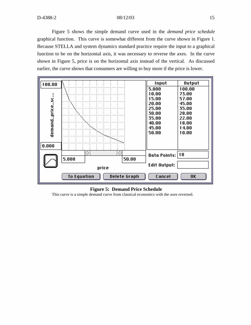
Figure 5 shows the simple demand curve used in the demand price schedule

graphical function. This curve is somewhat different from the curve shown in Figure 1.

Because STELLA and system dynamics standard practice require the input to a graphical

function to be on the horizontal axis, it was necessary to reverse the axes. In the curve

shown in Figure 5, price is on the horizontal axis instead of the vertical. As discussed

earlier, the curve shows that consumers are willing to buy more if the price is lower.

Figure 5: Demand Price ScheduleThis curve is a simple demand curve from classical economics with the axes reversed.

11:24 PM 08/12/03 D-4388-216

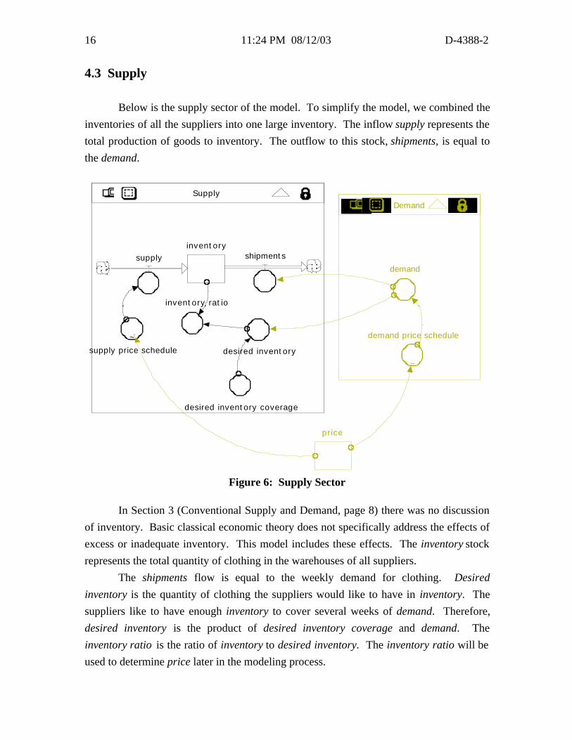
4.3 Supply

Below is the supply sector of the model. To simplify the model, we combined the

inventories of all the suppliers into one large inventory. The inflow supply represents the

total production of goods to inventory. The outflow to this stock, shipments, is equal to

the demand.

inventorysupply shipments

price

~


demand

~

supply price schedule

inventory ratio

desired inventory

desired inventory coverage

SupplyDemand

Figure 6: Supply Sector

In Section 3 (Conventional Supply and Demand, page 8) there was no discussion

of inventory. Basic classical economic theory does not specifically address the effects of

excess or inadequate inventory. This model includes these effects. The inventory stock

represents the total quantity of clothing in the warehouses of all suppliers.

The shipments flow is equal to the weekly demand for clothing. Desired

inventory is the quantity of clothing the suppliers would like to have in inventory. The

suppliers like to have enough inventory to cover several weeks of demand. Therefore,

desired inventory is the product of desired inventory coverage and demand. The

inventory ratio is the ratio of inventory to desired inventory. The inventory ratio will be

used to determine price later in the modeling process.

D-4388-2 08/12/03 17

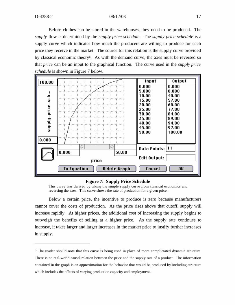
Before clothes can be stored in the warehouses, they need to be produced. The

supply flow is determined by the supply price schedule. The supply price schedule is a

supply curve which indicates how much the producers are willing to produce for each

price they receive in the market. The source for this relation is the supply curve provided

by classical economic theory6. As with the demand curve, the axes must be reversed so

that price can be an input to the graphical function. The curve used in the supply price

schedule is shown in Figure 7 below.

Figure 7: Supply Price ScheduleThis curve was derived by taking the simple supply curve from classical economics andreversing the axes. This curve shows the rate of production for a given price.

Below a certain price, the incentive to produce is zero because manufacturers

cannot cover the costs of production. As the price rises above that cutoff, supply will

increase rapidly. At higher prices, the additional cost of increasing the supply begins to

outweigh the benefits of selling at a higher price. As the supply rate continues to

increase, it takes larger and larger increases in the market price to justify further increases

in supply.

6 The reader should note that this curve is being used in place of more complictated dynamic structure.

There is no real-world causal relation between the price and the supply rate of a product. The information

contained in the graph is an approximation for the behavior that would be produced by including structure

which includes the effects of varying production capacity and employment.

11:24 PM 08/12/03 D-4388-218

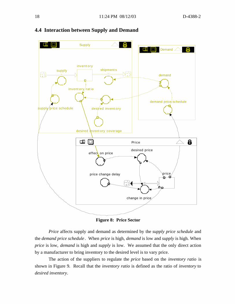
4.4 Interaction between Supply and Demand


price

change in price

~


demand

~


inventory ratio

~

effect on price

price change delay

desired inventory


desired price

Supply

Price

Demand

Figure 8: Price Sector

Price affects supply and demand as determined by the supply price schedule and

the demand price schedule . When price is high, demand is low and supply is high. When

price is low, demand is high and supply is low. We assumed that the only direct action

by a manufacturer to bring inventory to the desired level is to vary price.

The action of the suppliers to regulate the price based on the inventory ratio is

shown in Figure 9. Recall that the inventory ratio is defined as the ratio of inventory to

desired inventory.

D-4388-2 08/12/03 19

Figure 9: Effect on Price graphical functionWhen there is excess inventory, the price is lowered and when there is inadequateinventory, the price is raised.

The graphical function shown in Figure 9 represents the action of suppliers to

regulate their inventory. When inventory is below the desired inventory, then the

inventory ratio is less than one. The graph in Figure 9 shows that an inventory ratio less

than 1 gives a value for effect on price that is greater than one. This causes the price to

increase. The increase in price causes the supply to increase and the demand to decrease

through their respective price schedules and brings the inventory closer the desired value.

Multiplying the output of the effect on price converter and actual price returns desired

price.

Price was modeled as a stock because prices cannot change instantaneously.

People do not have immediate and exact information on the supply (inventory) and

demand of the commodity in question. Additionally, when the information becomes

available, it takes time to make a decision about changing the price.

11:24 PM 08/12/03 D-4388-220

5. TESTING THE MODEL

Putting the model together, we get the following:


price

change in price

~


demand

~


Inventory Ratio

~

effect on price

price change delay

desired inventory


desired price

Supply and Demand

Supply

Price

Demand

Figure 10: The complete Supply and Demand model

D-4388-2 08/12/03 21

At this point, you may wish to build the STELLA model of supply and demand.

The exercises that follow do not require you to run the model, but you may wish to

perform some simulations of your own. The complete model equations are included in

the appendix, beginning on page 33.

You will analyze three scenarios in this section. The first scenario will be a base

case run to observe the response of the model to a step increase in demand. Then you

will analyze how the behavior of the system varies from the base case when you change

the desired inventory coverage and the price change delay. Solutions start on page 28.

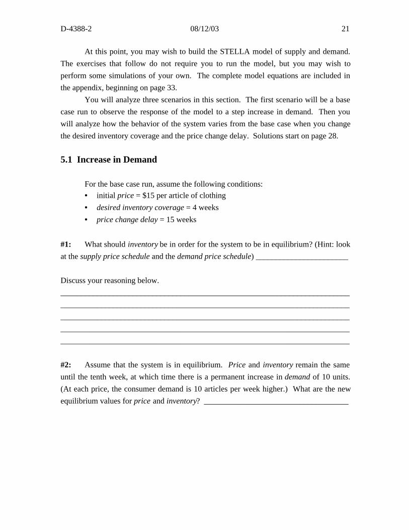
5.1 Increase in Demand

For the base case run, assume the following conditions:

• initial price = $15 per article of clothing

• desired inventory coverage = 4 weeks

• price change delay = 15 weeks

#1: What should inventory be in order for the system to be in equilibrium? (Hint: look

at the supply price schedule and the demand price schedule) _______________________

Discuss your reasoning below.

________________________________________________________________________

________________________________________________________________________

________________________________________________________________________

________________________________________________________________________

________________________________________________________________________

#2: Assume that the system is in equilibrium. Price and inventory remain the same

until the tenth week, at which time there is a permanent increase in demand of 10 units.

(At each price, the consumer demand is 10 articles per week higher.) What are the new

equilibrium values for price and inventory? ____________________________________

11:24 PM 08/12/03 D-4388-222

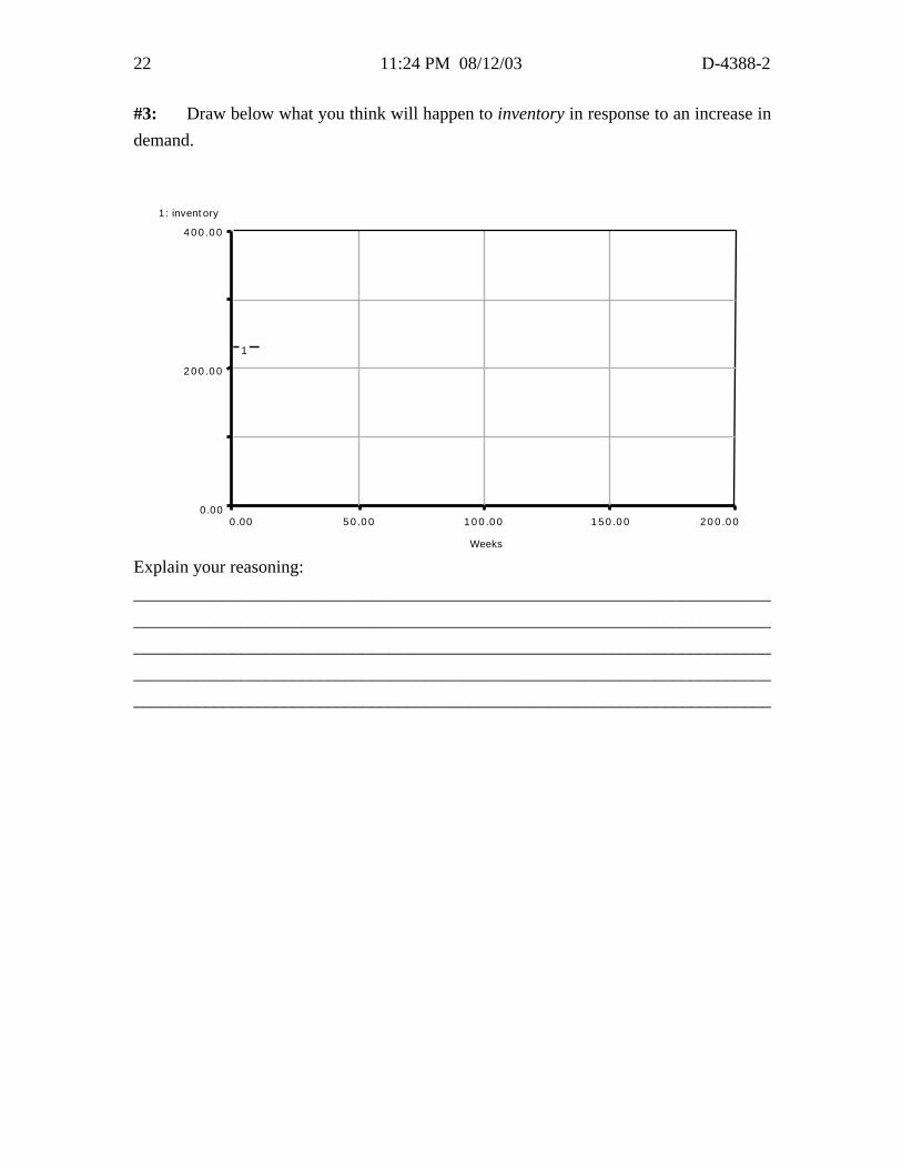
#3: Draw below what you think will happen to inventory in response to an increase in

demand.

0.00 50.00 100.00 150.00 200.00

Weeks

0.00

200.00

400.00

1: inventory

1

Explain your reasoning:

________________________________________________________________________

________________________________________________________________________

________________________________________________________________________

________________________________________________________________________

________________________________________________________________________

D-4388-2 08/12/03 23

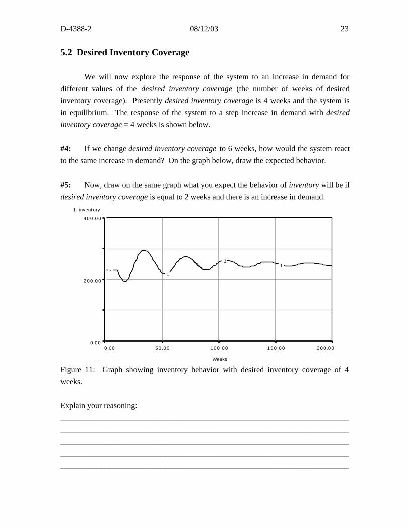
5.2 Desired Inventory Coverage

We will now explore the response of the system to an increase in demand for

different values of the desired inventory coverage (the number of weeks of desired

inventory coverage). Presently desired inventory coverage is 4 weeks and the system is

in equilibrium. The response of the system to a step increase in demand with desired

inventory coverage = 4 weeks is shown below.

#4: If we change desired inventory coverage to 6 weeks, how would the system react

to the same increase in demand? On the graph below, draw the expected behavior.

#5: Now, draw on the same graph what you expect the behavior of inventory will be if

desired inventory coverage is equal to 2 weeks and there is an increase in demand.

0.00 50.00 100.00 150.00 200.00

Weeks

0.00

200.00

400.00

1: inventory

1 1

11

Figure 11: Graph showing inventory behavior with desired inventory coverage of 4

weeks.


________________________________________________________________________

________________________________________________________________________

________________________________________________________________________

________________________________________________________________________

________________________________________________________________________

11:24 PM 08/12/03 D-4388-224

5.3 Price Change Delay

We are now ready to discuss the effect of varying the price change delay. The

delay obviously affects how quickly the price changes, and in the following exercises we

will see how well you can predict the behavior of price when that delay is modified.

#6: Currently, the price change delay is 15 weeks. Assuming everything else remains

unchanged (system in equilibrium), would price or inventory change over time if the

delay is suddenly shortened? __________________

Why or why not?

________________________________________________________________________

________________________________________________________________________

________________________________________________________________________

________________________________________________________________________

________________________________________________________________________

#7: Would you expect the system to reach equilibrium more quickly when the price

change delay is equal to 30 weeks or 15 weeks? ____________


________________________________________________________________________

________________________________________________________________________

________________________________________________________________________

________________________________________________________________________

________________________________________________________________________

D-4388-2 08/12/03 25

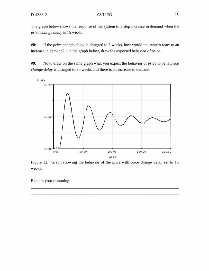
The graph below shows the response of the system to a step increase in demand when the

price change delay is 15 weeks.

#8: If the price change delay is changed to 5 weeks, how would the system react to an

increase in demand? On the graph below, draw the expected behavior of price.

#9: Now, draw on the same graph what you expect the behavior of price to be if price

change delay is changed to 30 weeks and there is an increase in demand.

0.00 50.00 100.00 150.00 200.00

Weeks

15.00

17.50

20.00

1: price

1

1

1

1

Figure 12: Graph showing the behavior of the price with price change delay set to 15

weeks.


________________________________________________________________________

________________________________________________________________________

________________________________________________________________________

________________________________________________________________________

________________________________________________________________________

11:24 PM 08/12/03 D-4388-226

5.4 Further Exploration

Naturally, no system dynamics model is ever complete. We believe that the

model presented is adequate for the purposes of this paper, but there are many

possibilities for enhancing it. One possibility is to include the effect of available

inventory on demand. The current model assumes that if a product is not currently

available, the consumer will simply place an order and wait for the product to arrive,

creating negative inventory, or backlog. You may also wish to include structure for

increasing the capacity of the supplier. This would allow for increased production

without raising the per-item cost. You could also experiment with the dynamics of a non-

durable good market (i.e., food). The possibilities are unlimited and it will help enhance

your modeling skills.

D-4388-2 08/12/03 27

6. SOLUTIONS TO EXERCISES

6.1 Increase in Demand

#1: In equilibrium, all stocks must remain constant. The price will remain constant

when the inventory ratio is one. Therefore, in equilibrium, the inventory is equal to the

desired inventory. By looking at the supply and demand curves contained in the

graphical functions of Demand Price Schedule and Supply Price Schedule we can see that

the equilibrium price is $15 when demand and production both equal 57 articles of

clothing per week. Since the desired inventory coverage is 4 weeks, the equilibrium

inventory is 228 articles of clothing.

#2: An increase in demand of 10 articles of clothing per week means that the demand

curve in the demand price schedule is shifted up by 10. An easy way to figure out the

new equilibrium price is to plot the supply curve and the new demand curve on the same

graph and find the intersection. Doing this shows that the new equilibrium price will be

about $17 with production and demand slightly less than 62 articles per week. The new

equilibrium inventory is then 62*4 or 248 articles of clothing.

11:24 PM 08/12/03 D-4388-228

0.00 50.00 100.00 150.00 200.00

Weeks

0.00

200.00

400.00

1: inventory

1 1

11

Figure 13: Step in DemandInventory decreases at first due to increased demand. It then overshoots and oscillates toa new equilibrium.

#3: The increase in demand causes the desired inventory to immediately shoot up by

40 articles of clothing (10 articles per week * 4 weeks of coverage). At the same time,

inventory begins to drop because shipments are higher than supply. These cause the

inventory ratio to drop, resulting in an increase in price. The price increase causes the

demand to fall and supply to increase allowing the inventory to catch up to the desired

inventory. However, the price continues to rise until the inventory has overshot its

equilibrium value. At this point the inventory ratio becomes positive, causing the price to

begin falling. Although the price is falling, it remains above its equilibrium value

causing the inventory to continue increasing beyond its equilibrium. Eventually, the

price falls below the equilbrium price and causes the inventory to begin decreasing, but

the inventory again overshoots and the system oscillates to its new equilibrium with

inventory equal to about 248. A graph of this behavior is shown in Figure 11.

D-4388-2 08/12/03 29

6.2 Desired Inventory Coverage

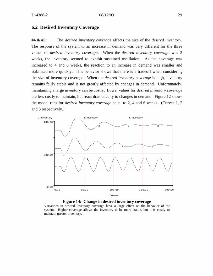
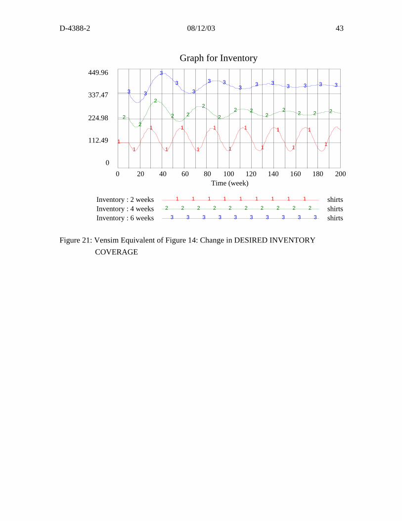
#4 & #5: The desired inventory coverage affects the size of the desired inventory.

The response of the system to an increase in demand was very different for the three

values of desired inventory coverage. When the desired inventory coverage was 2

weeks, the inventory seemed to exhibit sustained oscillation. As the coverage was

increased to 4 and 6 weeks, the reaction to an increase in demand was smaller and

stabilized more quickly. This behavior shows that there is a tradeoff when considering

the size of inventory coverage. When the desired inventory coverage is high, inventory

remains fairly stable and is not greatly affected by changes in demand. Unfortunately,

maintaining a large inventory can be costly. Lower values for desired inventory coverage

are less costly to maintain, but react dramatically to changes in demand. Figure 12 shows

the model runs for desired inventory coverage equal to 2, 4 and 6 weeks. (Curves 1, 2

and 3 respectively.)

0.00 50.00 100.00 150.00 200.00

Weeks

0.00

200.00

400.00

1: inventory 2: inventory 3: inventory

1

1 1 1

2

22 2

3

3 3 3

Figure 14: Change in desired inventory coverageVariations in desired inventory coverage have a large effect on the behavior of thesystem. Higher coverage allows the inventory to be more stable, but it is costly tomaintain greater inventory.

11:24 PM 08/12/03 D-4388-230

6.3 Price Change Delay

#6: The price change delay does not affect the equilibrium state of the model. This

delay only comes into effect when the price is changing. Any change in the price change

delay will not affect the model if it is already in equilibrium.

#7: When the model is knocked out of equilibrium, the price change delay affects

how it approaches its new equilibrium. When the price change delay is short (5 weeks),

the price changes rapidly and overshoots its equilibrium value. The price also converges

on its equilibrium quickly. As the price change delay increases (15 weeks and 30

weeks), the changes are more gradual, the overshoot smaller and the equilibrium takes

longer to reach.

D-4388-2 08/12/03 31

#8, #9: The graphs below show the reaction of price to an increase in demand when the

price change delay is 5, 15 and 30 weeks.

0.00 50.00 100.00 150.00 200.00

Weeks

15.00

17.50

20.00

1: price

1

1

1

1

0.00 50.00 100.00 150.00 200.00

Weeks

15.00

17.50

20.00

1: price

1

1 1 1

0.00 50.00 100.00 150.00 200.00

Weeks

15.00

17.50

20.00

1: price

1

1

1

1

5 Weeks

15 Weeks

30 Weeks

Figure 15: Variations in price change delay

11:24 PM 08/12/03 D-4388-232

7. APPENDIX

7.1 Model Equations

Demand Sector

demand = demand_price_schedule+step(10,10)DOCUMENT: This is the rate at which consumers wish to purchase clothing from thecompany. The step function is used to jar the system out of equilibrium.UNITS: shirts per week

demand_price_schedule = GRAPH(price)(5.00, 100), (10.0, 73.0), (15.0, 57.0), (20.0, 45.0), (25.0, 35.0), (30.0, 28.0), (35.0, 22.0),(40.0, 18.0), (45.0, 14.0), (50.0, 10.0)DOCUMENT: This is based on the simple demand curve. At some particular price, theconsumers are willing and able to purchase clothing at a certain rate; the lower the price,the higher the demand.UNITS: shirts per week

Price Sector

price(t) = price(t - dt) + (change_in_price) * dtINIT price = 15DOCUMENT: Price is modeled as a stock in order to model the delays inherent inchanges in price.UNITS : dollars per shirt

INFLOWS:

change_in_price = ((desired_price)-price)/price_change_delayDOCUMENT: Change in price can be either positive or negative depending onthe effect_on_price. If the effect_on_price > 1, then price will increase. If theeffect_on_price < 1, then the price decreases. If effect_on_price = 1, priceremains same. Price changes slowly, so we divide the change byprice_change_delay.UNITS: price/week or ($/shirt)/week

desired_price = effect_on_price*priceDOCUMENT: This is the equilibrium price as set by the inventory_ratio. The actualprice will reach this value after a delay specified by the price_change_delay.UNITS: dollars per shirt

price_change_delay = 15DOCUMENT: Prices do not change instantaneously. This value determines howquickly price can change.UNITS : weekseffect_on_price = GRAPH(inventory_ratio)(0.5, 2.00), (0.6, 1.80), (0.7, 1.55), (0.8, 1.35), (0.9, 1.15), (1, 1.00), (1.10, 0.875), (1.20,0.75), (1.30, 0.65), (1.40, 0.55), (1.50, 0.5)DOCUMENT: This graphical function regulates price change. When the inventory >desired_inventory then the inventory_ratio is >1 and price must be reduced. When theinventory ratio is <1, price must be increased.

D-4388-2 08/12/03 33

UNITS: dimensionless

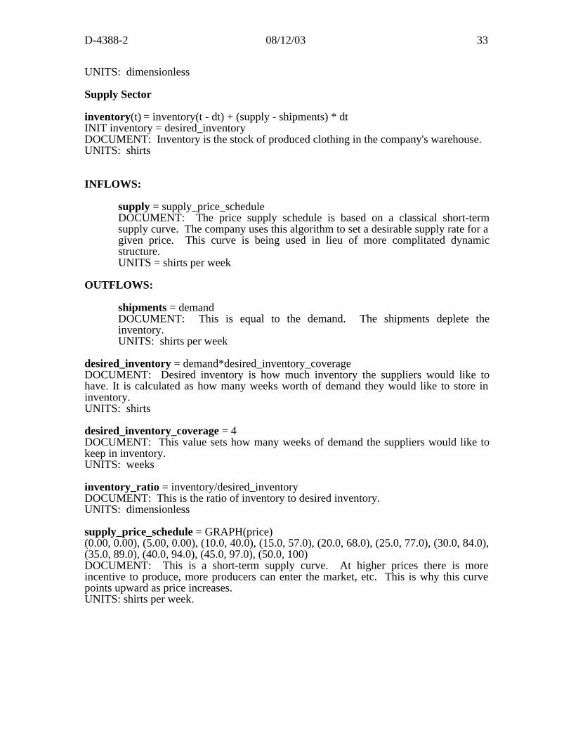
Supply Sector

inventory(t) = inventory(t - dt) + (supply - shipments) * dtINIT inventory = desired_inventoryDOCUMENT: Inventory is the stock of produced clothing in the company's warehouse.UNITS: shirts

INFLOWS:

supply = supply_price_scheduleDOCUMENT: The price supply schedule is based on a classical short-termsupply curve. The company uses this algorithm to set a desirable supply rate for agiven price. This curve is being used in lieu of more complitated dynamicstructure.UNITS = shirts per week

OUTFLOWS:

shipments = demandDOCUMENT: This is equal to the demand. The shipments deplete theinventory.UNITS: shirts per week

desired_inventory = demand*desired_inventory_coverageDOCUMENT: Desired inventory is how much inventory the suppliers would like tohave. It is calculated as how many weeks worth of demand they would like to store ininventory.UNITS: shirts

desired_inventory_coverage = 4DOCUMENT: This value sets how many weeks of demand the suppliers would like tokeep in inventory.UNITS: weeks

inventory_ratio = inventory/desired_inventoryDOCUMENT: This is the ratio of inventory to desired inventory.UNITS: dimensionless

supply_price_schedule = GRAPH(price)(0.00, 0.00), (5.00, 0.00), (10.0, 40.0), (15.0, 57.0), (20.0, 68.0), (25.0, 77.0), (30.0, 84.0),(35.0, 89.0), (40.0, 94.0), (45.0, 97.0), (50.0, 100)DOCUMENT: This is a short-term supply curve. At higher prices there is moreincentive to produce, more producers can enter the market, etc. This is why this curvepoints upward as price increases.UNITS: shirts per week.

11:24 PM 08/12/03 D-4388-234

7.2 Typical Model Behavior

These graphs represent the behavior of the model set up with the values in the

equations listed above. The model is initialized in equilibrium and there is a step increase

in demand of 10 units/week after 10 weeks.

0.00 50.00 100.00 150.00 200.00

Weeks

0.00

200.00

400.00

0.00

1.50

3.00

1: inventory 2: desired inventory 3: inventory ratio

11

11

22

2 2

3 33 3

0.00 50.00 100.00 150.00 200.00

Weeks

50.00

60.00

70.00

1: shipments 2: supply

1

11

1

2

2

2

2

D-4388-2 08/12/03 35

0.00 50.00 100.00 150.00 200.00

Weeks

10.00

20.00

30.00

1: price 2: desired price

1

1 1 1

2

22

2

Figure 16: Graphs of Typical Model Behavior with parameters set to values in the model

equations.

11:24 PM 08/12/03 D-4388-236

Vensim Examples:Economic Supply & Demand

By Lei Lei & Nathaniel Choge

February 2001

Supply and Demand

Figure 17: Vensim Equivalent of Figure 10: The complete Supply and Demand model

Documentation for Complete Supply and Demand Model

(01) change in price = (desired price-Price)/PRICE CHANGE DELAY

Units: (dollars/shirt)/week

Change in price can be either positive or negative depending on the effect on

price. If the effect is >1, then price will increase. If the effect < 1, the price

decreases. If effect = 1, price remains the same. Price changes slowly, so we

divide the change by price change delay.

Inventorysupply shipments

Price

inventory ratio

demand

desiredinventory

DESIREDINVENTORYCOVERAGE

demand priceschedule

DEMAND PRICE LOOKUP

desired price

effect on price

EFFECT ONPRICE LOOKUP


SUPPLY PRICE LOOKUP

change in price

PRICE CHANGE DELAY

INITIAL PRICE

NORMALDEMAND

price ratio

NORMALSUPPLY

D-4388-2 08/12/03 37

(02) demand = demand price schedule* NORMAL DEMAND+STEP(10,10)

Units: shirts/week

This is the rate at which consumers wish to purchase clothing from the company.

The step function is used to jar the system out of equilibrium.

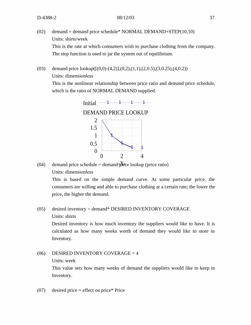
(03) demand price lookup([(0,0)-(4,2)],(0,2),(1,1),(2,0.5),(3,0.25),(4,0.2))

Units: dimensionless

This is the nonlinear relationship between price ratio and demand price schedule,

which is the ratio of NORMAL DEMAND supplied.

(04) demand price schedule = demand price lookup (price ratio)


This is based on the simple demand curve. At some particular price, the

consumers are willing and able to purchase clothing at a certain rate; the lower the

price, the higher the demand.

(05) desired inventory = demand* DESIRED INVENTORY COVERAGE

Units: shirts

Desired inventory is how much inventory the suppliers would like to have. It is

calculated as how many weeks worth of demand they would like to store in

Inventory.

(06) DESIRED INVENTORY COVERAGE = 4

Units: week

This value sets how many weeks of demand the suppliers would like to keep in

Inventory.

(07) desired price = effect on price* Price

Initial 1 1 1 1

DEMAND PRICE LOOKUP2

1.51

0.50

1

11 1

0 2 4-X-

11:24 PM 08/12/03 D-4388-238

Units: dollars/shirt

This is the equilibrium price as set by the inventory ratio. The actual price will

reach this value after a delay specified by the PRICE CHANGE DELAY.

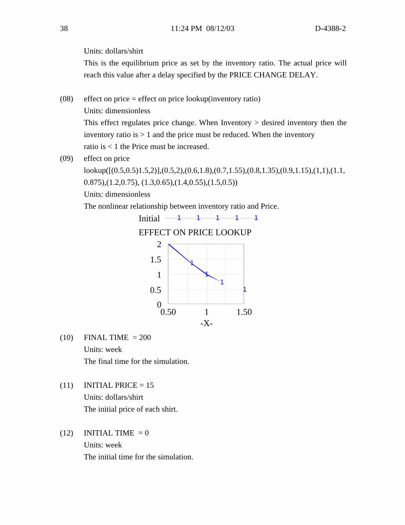
(08) effect on price = effect on price lookup(inventory ratio)


This effect regulates price change. When Inventory > desired inventory then the

inventory ratio is > 1 and the price must be reduced. When the inventory

ratio is < 1 the Price must be increased.

(09) effect on price

lookup([(0.5,0.5)1.5,2)],(0.5,2),(0.6,1.8),(0.7,1.55),(0.8,1.35),(0.9,1.15),(1,1),(1.1,

0.875),(1.2,0.75), (1.3,0.65),(1.4,0.55),(1.5,0.5))


The nonlinear relationship between inventory ratio and Price.

(10) FINAL TIME = 200

Units: week

The final time for the simulation.

(11) INITIAL PRICE = 15


The initial price of each shirt.

(12) INITIAL TIME = 0

Units: week

The initial time for the simulation.

Initial 1 1 1 1 1

EFFECT ON PRICE LOOKUP2

1.5

1

0.5

0

1

11

1

0.50 1 1.50-X-

D-4388-2 08/12/03 39

(13) Inventory = INTEG (+supply-shipments, desired inventory)

Units: shirts

Inventory is the stock of produced clothing in the company's warehouse.

(14) inventory ratio = Inventory/ desired inventory


This is the ratio of Inventory to desired inventory.

(15) NORMAL DEMAND = 57

Units: shirts/week

The normal number of shirts customers demand per week.

(16) NORMAL SUPPLY= 57

Units: shirts/week

The normal number of shirts per week that can be supplied.

(17) Price = INTEG (change in price, INITIAL PRICE)


Price is modeled as a stock in order to model the delays inherent in changes in

Price.

(18) PRICE CHANGE DELAY = 15

Units: week

Prices do not change instantaneously. This value determines how quickly Price

can change.

(19) price ratio = Price/ INITIAL PRICE


The ratio of Price over INITIAL PRICE.

(20) SAVEPER = TIME STEP

Units: week

The frequency with which output is stored.

(21) shipments = demand

Units: shirts/week

11:24 PM 08/12/03 D-4388-240

This is equal to the demand. The shipments deplete the Inventory.

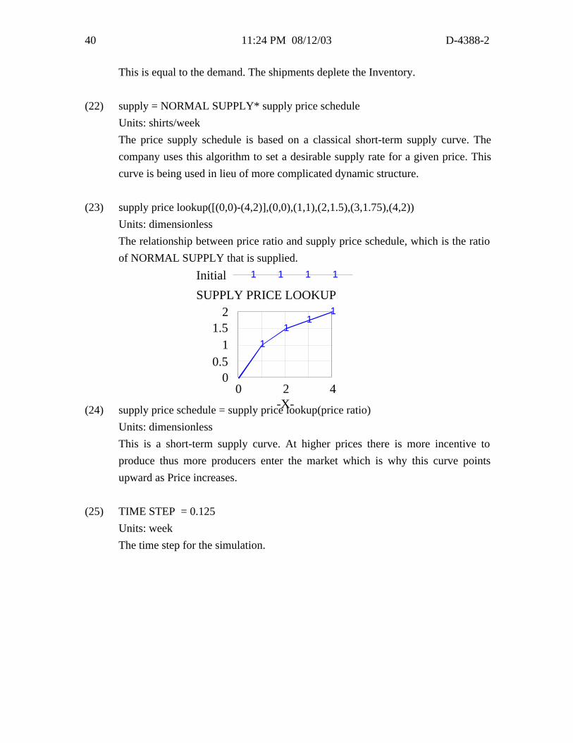
(22) supply = NORMAL SUPPLY* supply price schedule

Units: shirts/week

The price supply schedule is based on a classical short-term supply curve. The

company uses this algorithm to set a desirable supply rate for a given price. This

curve is being used in lieu of more complicated dynamic structure.

(23) supply price lookup([(0,0)-(4,2)],(0,0),(1,1),(2,1.5),(3,1.75),(4,2))


The relationship between price ratio and supply price schedule, which is the ratio

of NORMAL SUPPLY that is supplied.

(24) supply price schedule = supply price lookup(price ratio)


This is a short-term supply curve. At higher prices there is more incentive to

produce thus more producers enter the market which is why this curve points

upward as Price increases.

(25) TIME STEP = 0.125

Units: week

The time step for the simulation.

Initial 1 1 1 1

SUPPLY PRICE LOOKUP2

1.51

0.50

1

11

1

0 2 4-X-

D-4388-2 08/12/03 41

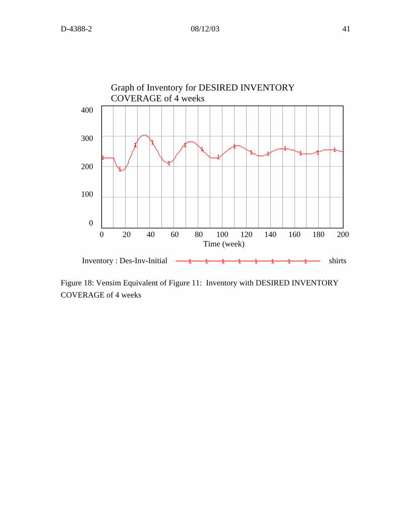
Figure 18: Vensim Equivalent of Figure 11: Inventory with DESIRED INVENTORY

COVERAGE of 4 weeks

Graph of Inventory for DESIRED INVENTORYCOVERAGE of 4 weeks

400

300

200

100

0

1

1

1 1

1

11

1

11 1

11 1 1

0 20 40 60 80 100 120 140 160 180 200Time (week)

Inventory : Des-Inv-Initial shirts1 1 1 1 1 1 1 1

11:24 PM 08/12/03 D-4388-242

Figure 19: Vensim Equiv. of Figure 12: Simulation for Price with PRICE CHANGE

DELAY of 15 weeks

Figure 20: Vensim Equivalent of Figure 13: Step in Demand

Graph of Price with PRICE CHANGE DELAY at 15 weeks

21

19.5

18

16.5

151

1

1

1

11

1

1

1

1

1

1 1

1

1

0 20 40 60 80 100 120 140 160 180 200Time (week)

Price : Des-Inv-Initial dollars/shirt1 1 1 1 1 1 1 1

Step in Demand

400

200

0

1

1

1

11 1

11

11 1 1 1

0 20 40 60 80 100 120 140 160 180 200Time (week)

Inventory : Step shirts1 1 1 1 1 1 1 1

D-4388-2 08/12/03 43

Figure 21: Vensim Equivalent of Figure 14: Change in DESIRED INVENTORY

COVERAGE

Graph for Inventory

449.96

337.47

224.98

112.49

0

3 3

3

3

3

3 33

3 33 3 3 3

22

2

2 2

2

22 2

22

2 2 2

1

1

1

1

1

1

1

1

1

1

1

1

1

1

0 20 40 60 80 100 120 140 160 180 200Time (week)

Inventory : 2 weeks shirts1 1 1 1 1 1 1 1 1

Inventory : 4 weeks shirts2 2 2 2 2 2 2 2 2 2

Inventory : 6 weeks shirts3 3 3 3 3 3 3 3 3 3

11:24 PM 08/12/03 D-4388-244

Graph of Price with Price Change Delay of 30 weeks21

19.5

18

16.5

151

1

1

1

1

1

1

1

11

1

11

11

0 20 40 60 80 100 120 140 160 180 200Time (week)

Price : current dollars/shirt1 1 1 1 1 1 1 1 1

Graphs showing the reaction of price to increase in demand when price change delay is 5,

15 and 30 weeks.

Figure 22: Vensim Equivalent of Figure 15: Variations in PRICE CHANGE DELAY

Graph of Price with PRICE CHANGE DELAY of 5 weeks

21

19.5

18

16.5

151

1

1

1

1 11

1 1 1 1 1 1 1 1

0 20 40 60 80 100 120 140 160 180 200Time (week)


Graph of Price with Price Change Delay of 15 weeks21

19.5

18

16.5

151

1

1

1

11

1

1

1

1

1

1 11

1

0 20 40 60 80 100 120 140 160 180 200Time (week)


D-4388-2 08/12/03 45

Model set up with initial values from the equations listed above, initialized at equilibrium

with step increase in demand of 10 units/week after 10 weeks.

Graph of Inventory, Desired Inventory, and Inventory Ratio400 shirts

400 shirts

3 dimensionless

0 shirts

0 shirts

0 dimensionless

3

33 3

33

33 3 3 3 3

2 22 2 2 2 2 2 2 2 2 2

1

1

1

1

1 11

11

1 1 1 1

0 20 40 60 80 100 120 140 160 180 200Time (week)

Inventory : Initial shirts1 1 1 1 1 1 1 1 1 1 1

desired inventory : Initial shirts2 2 2 2 2 2 2 2 2

inventory ratio : Initial dimensionless3 3 3 3 3 3 3 3 3

Graph of Shipments and Supply

70 shirts/week70 shirts/week



2

2

2

2

2

2

22

22

11

1

1

1

1

11

11

1

0 30 60 90 120 150 180Time (week)

shipments : Initial shirts/week1 1 1 1 1 1 1

supply : Initial shirts/week2 2 2 2 2 2 2 2

11:24 PM 08/12/03 D-4388-246

Figure 23: Vensim equivalent of figure 16: Typical model behavior when set to initial

conditions.

Graph of Price and Desired Price

30 dollars/shirt30 dollars/shirt



22

22

22

2 22 2

1

1

1

1

11

11

1 1 1

0 30 60 90 120 150 180Time (week)

Price : Initial dollars/shirt1 1 1 1 1 1 1 1

desired price : Initial dollars/shirt2 2 2 2 2 2 2

ECONOMIC SUPPLY & DEMAND - The Creative...

Documents

Transcript of ECONOMIC SUPPLY & DEMAND - The Creative...