economic motivation for variance contracts revised · PDF fileAn Economic Motivation for...

An Economic Motivation for Variance Contracts

Nicole Branger§ Christian Schlag‡

This version: December 31, 2005

§Department of Business and Economics, University of Southern Denmark, Campusvej 55, DK-5230Odense M, Denmark. E-mail: [email protected]

‡Finance Department, Goethe University, Mertonstr. 17-21/Uni-Pf 77, D-60054 Frankfurt am Main,Germany. E-mail: [email protected]



Abstract

Variance contracts permit the trading of ’variance risk’, i.e. the risk that the realizedvariance of stock returns changes randomly over time. We discuss why investorsmight want to trade this type of risk, and why they might prefer a variance contractto standard calls and puts for this purpose.

Our main argument is that the variance contract is superior to a dynamic replicationstrategy due to parameter risk, and model risk. To show this we analyze the localhedging errors for the variance contract under different scenarios, namely underpure estimation risk (or parameter risk) in a stochastic volatility and in a jump-diffusion model, under model risk when the wrong type of risk factor is assumed tobe present (stochastic volatility instead of jumps or vice versa), and under modelrisk when risk factors are omitted (e.g. when the true model contains jumps whichare not present in the model assumed by the investor). The results show that thevariance contract is exposed to model risk to an economically significant degree,and that it is much harder to hedge than, e.g., deep OTM puts. We also show thatthe semi-static replication strategy which builds on the log-contract fails in case ofjumps. Our conclusion is that the improvement provided by the introduction of avariance contract is greater than the one offered by the introduction of additionalstandard options.

Keywords: Variance Risk, Stochastic Volatility, Jump-Diffusion, Model Risk, Pa-rameter Risk, Hedging Error

JEL: G12, G13


Nicole Branger§ Christian Schlag‡


Abstract

Variance contracts permit the trading of ’variance risk’, i.e. the risk that the realizedvariance of stock returns changes randomly over time. We discuss why investorsmight want to trade this type of risk, and why they might prefer a variance contractto standard calls and puts for this purpose.

Our main argument is that the variance contract is superior to a dynamic replicationstrategy due to parameter risk, and model risk. To show this we analyze the localhedging errors for the variance contract under different scenarios, namely underpure estimation risk (or parameter risk) in a stochastic volatility and in a jump-diffusion model, under model risk when the wrong type of risk factor is assumed tobe present (stochastic volatility instead of jumps or vice versa), and under modelrisk when risk factors are omitted (e.g. when the true model contains jumps whichare not present in the model assumed by the investor). The results show that thevariance contract is exposed to model risk to an economically significant degree,and that it is much harder to hedge than, e.g., deep OTM puts. We also show thatthe semi-static replication strategy which builds on the log-contract fails in case ofjumps. Our conclusion is that the improvement provided by the introduction of avariance contract is greater than the one offered by the introduction of additionalstandard options.

Keywords: Variance Risk, Stochastic Volatility, Jump-Diffusion, Model Risk, Pa-rameter Risk, Hedging Error

JEL: G12, G13

§Department of Business and Economics, University of Southern Denmark, Campusvej 55, DK-5230Odense M, Denmark. E-mail: [email protected]

‡Finance Department, Goethe University, Mertonstr. 17-21/Uni-Pf 77, D-60054 Frankfurt am Main,Germany. E-mail: [email protected]

1 Introduction and Motivation

There is ample evidence from empirical studies of option markets that there are additionalpriced factors beyond plain stock price risk (see, e.g., Bakshi, Cao, and Chen (1997),Bates (2000), Pan (2002), and Eraker (2004)). Therefore, extensions of the seminal modeldeveloped by Black and Scholes (1973) contain factors like stochastic volatility (SV) orstochastic jumps (SJ). The presence of these additional factors makes markets incomplete,so that trading in the stock and the money market account is not enough to replicate anarbitrary derivative payoff or to realize the optimal consumption stream. For this purposemore contracts are needed. This insight is probably the most important motivation for theintroduction of innovative derivatives like variance contracts, which recently took placeon major exchanges like the CBOE, as described in Bondarenko (2004).

A variance contract permits the trading of the stochastic variation of stock returnvolatility by basically paying off the sum of squared price changes. The larger the realizedvariance of the stock due to increases in stochastic volatility or jumps in the stock price, thehigher the payoff of the variance contract. It therefore allows speculation on the amount ofrisk represented by the stock over a certain period of time. In this paper, we first providea detailed discussion of the risk exposure of the variance contract and we discuss differentcompeting explanations for the significantly negative risk premium which is documentedin empirical studies, e.g. in Bondarenko (2004). Second, we provide economic argumentsfor the introduction of the variance contract by an exchange.

The first question we address is why investors would want to trade volatility risk andjump risk in addition to trading stock price risk. The standard answer lists two mainmotives: speculation and hedging. If the market price of risk for a risk factor is differentfrom zero, the investor trades this risk factor to earn the risk premium. Furthermore, riskfactors like stochastic volatility may have an impact on future investment opportunities,that is on future interest rates and/or market prices of risk which then change randomlyover time. The investor takes this stochastic behavior into account when planning hisportfolio by taking some long or short positions in the respective risk factors, whichMerton (1971) called ’hedging demand’. Note, however, that this hedging motive is notexactly the same as the one related to the risk management of a derivative position.Especially, we do not claim that investors mainly use the variance contract to hedge vegarisk in their option books.

Liu and Pan (2003) solve a portfolio planning problem in a partial equilibrium modelwith stochastic volatility and jumps (of deterministic size) in the stock price. Branger,Schlag, and Schneider (2005b) also include simultaneous jumps in volatility. They con-sider a complete market and derive the investor’s optimal exposure to stock price risk,volatility risk, and jump risk. Their results show that the investor wants to trade bothstochastic volatility and jump risk, and their results also allow to see under what circum-stances different investors would want to hold long and short positions in volatility risk.Branger, Schlag, and Schneider (2005a) analyze a general equilibrium setup and show thatheterogeneous agents will trade both stochastic volatility and jump risk. These findingsconfirm that there is indeed a demand for positions in variance risk.

1

Given this trading demand of the investors, the main part of our paper is dedicated tothe question why investors might be interested in the introduction of additional contracts,and why they might prefer the introduction of the variance contract to an augmentationof the set of available options. A natural first step seems to be to distinguish betweena complete and an incomplete market. If the market is incomplete, one reason for theintroduction of a variance contract could be that it is market-completing. However, thiswould also be true for an additional option. When too few contracts are traded, whyshould one introduce a rather complicated derivative asset like a variance contract insteadof additional simple European options? On the other hand, if the market is complete, thevariance contract can be replicated by a dynamic trading strategy, and this also holdsfor other new claims. There is no need to introduce further redundant claims, whichin addition would only take away liquidity from existing contracts. Summing up: In anincomplete market the variance contract does not seem to be the most natural contractto introduce, and in a complete market, there is no need to introduce it.

We thus have to explain why the variance contract is not necessarily redundant, i.e.why perfect replication is not possible, and we have to explain why there is more needto introduce the variance contract than some standard option. In this paper, we arguethat the ’replicating’ strategy may fail due to model risk, which makes it impossible forthe investor to know the correct composition of the hedge portfolio. In these cases, thevariance contract will be better than its ’replicating’ strategy, because the investor doesnot have to worry about the potentially difficult replication, but can buy the desiredpayoff directly.

Our ultimate line of argument for the variance contract then consists of three steps.First, a new contract should only be introduced if investors want to trade the payoff profileor risk exposure provided by this contingent claim. We argue that this condition holdsfor the variance contract. Second, the introduction makes sense only if the ’replicating’strategy for the new contract is subject to model risk to an economically significant extent,and we show that this is the case for the variance contract. Third, if there is still morethan one contract that could be introduced, the choice should be the one which is hardestto replicate. The main result of our analysis is indeed that the variance contract is muchharder to replicate than standard derivatives like a deep OTM put option.

We argue that the ’replicating’ strategy for the variance contract may fail due to modelrisk. The true data generating process is not known so that the replicating strategy willbe determined in some model (the hedge model), which is in general not equal to thetrue model. Thus, the dynamic replication strategy will be more risky than trading thecontract itself. Model risk can occur in different forms and to different degrees, and weconsider both the impact of parameter risk and model mis-specification. Parameter riskmeans that the correct type of model is used, but with incorrect parameters (possiblyderived from some estimation, so that parameter risk is basically equivalent to estimationrisk). A second form of model risk occurs when the wrong risk factors are included inthe hedge model. The most prominent example is to use a hedge model which contains astochastic volatility component, while the true model exhibits stochastic jumps (or viceversa). Finally, risk factors present in the true model may be omitted in the hedge model,

2

so that instead of stochastic volatility and stochastic jumps together only one of theserisk factors is included in the hedge model.

Besides dynamic hedging strategies, we have to consider a second class of hedgingstrategies for the variance contract, namely semi-static replication strategies discussed,e.g., by Neuberger (1994), Bondarenko (2004), Carr and Wu (2004) and Jiang and Tiang(2005). They show that for an underlying without jumps the variance contract is equal toa position in log-contracts (which can be statically replicated via a continuum of options),the money market account and some dynamic strategy in the underlying. In practice, thisapproach suffers from at least two problems. The first is the assumption that a continuumof options is available. Even if enough options are traded to price the variance contract, thisdoes not necessarily imply that the static hedge of the log-contract is of similar accuracy.Second, the hedge is perfect only for a certain class of models with deterministic interestrates and without jumps in the stock price, or, as shown by Bondarenko (2004) for thecase of jumps, if the contract specification is adjusted appropriately. Jump risk is thus aproblem and can only be dealt with by dynamic hedging strategies which are exposed tomodel risk.

Finally, it seems useful to consider the perspective of ’normal’ investors on the onehand and highly specialized financial institutions like hedge funds on the other hand.Normal investors interested in trading variance risk will prefer the direct investment intoa variance contract to a dynamic ’replicating’ strategy which may fail due to model risk,and also to the semi-static strategy described above, which is still exposed to jump risk.Highly specialized investors will have an advantage in replicating the variance contractand will therefore provide liquidity in this market. They use trading strategies whichinvolve a wide array of instruments anyway and which are based on highly sophisticatedmodels. It thus seems reasonable to assume that they will be quite successful in hedgingthe variance contract. Nevertheless, they are still exposed to model risk (to a smallerextent than ’normal’ investors), and they will basically compete with each other in termsof their modeling and hedging competence.

To analyze the impact of model risk on the replicating strategy we derive analyticalexpressions for local hedging errors over an infinitesimal time interval. The global hedgingerror over some interval from t to t+τ is then simply given by the integral over these localerrors, so that an analysis of local errors seems sufficient. We show that the hedging errordepends on the error in the sensitivities of the claim to be hedged with respect to the riskfactors, as well as on the error in the sensitivities of the hedge instruments. We also derivea robustness condition, under which the strategy would have a zero exposure to modelrisk, and which basically says that the two errors mentioned above should exactly offseteach other. Intuitively, we expect model risk to be only a moderate problem when theclaim to be hedged and the hedge instrument are very similar. To achieve a robust hedgefor the variance contract, there are two natural candidates, namely an ATM straddle (orATM option) and an OTM put. The ATM straddle is often considered an ideal instrumentfor volatility trading and could thus be used to hedge the exposure of the variance contractwith respect to volatility risk. The OTM put allows for the trading of downside jump riskand could therefore be used to hedge the jump risk exposure of the variance contract.

3

To concentrate on the main issues we make several simplifying assumptions. First, werestrict our analysis to the case where only the stock, the money market account, and onefurther option are already traded, and we choose the hedge models such that the marketis complete with this set of basis assets. The investor then uses the (unique) replicatingstrategy from the hedge model. In an incomplete market, one would have to decide whichhedge criterion (like super-hedging, variance minimization or quantile hedging) to use.In a complete market where too many assets are traded, on the other hand, one wouldhave to decide which assets to use in a dynamic strategy or which of the many replicatingstrategies to use. In both cases, the performance of the hedging strategies would thendepend on these additional choices. By our assumptions we avoid this dependence, whichallows us to focus directly on the impact of model mis-specification.

We rely on numerical examples to compare the exposures of different claims to modelrisk. In these examples the true model is given by Merton (1976) including jumps, thestochastic volatility model of Heston (1993), or the model of Bakshi, Cao, and Chen (1997)which includes both stochastic volatility and jumps. We assume that the jump sizes aredeterministic. The hedge model (which is either Merton (1976) or Heston (1993)) is thencalibrated to the prices of selected options, where we allow for small price deviations wellwithin the bid-ask-spread.

We will now give a brief summary of our results. In our hedging experiments the stock,the money market account, and standard European options with varying strike pricesare used as hedge instruments. We compare the hedging error for the variance contractto the hedging error for a deep out-of-the-money (OTM) put option. We have chosenthis instrument as the benchmark case, since it represents an example for a standardclaim, which might compete with the variance contract for introduction on a derivativesexchange. It is not surprising that the hedging error for this OTM put is the smaller thelower the difference between its strike and the strike of the option we use as the hedgeinstrument, which means that we can actually choose some best hedge instrument amongthe available contracts. For the variance contract the hedging errors are comparable insize to those observed for the benchmark put. However, the variance contract is moredifficult to hedge for two reasons. First, there is no ideal hedge instrument for whichthe hedging error due to model risk would vanish. Second, a hedge instrument whichprovides a good hedge for the variance contract in one scenario may perform ratherbadly in other scenarios, so there is no dominant choice of hedge instruments. In fact,it turns out that neither the ATM straddle nor the OTM put provide a robust hedge.Thus, the variance contract is exposed to model risk much more than a deep OTM putoption. The actual introduction of the variance contract is an improvement over thesituation when investors have to replicate its payoff using a traded option only, and itoffers a more significant improvement than a deep OTM put. In a nutshell, the variancecontract provides the easiest way to generate a positive exposure to increasing realizedstock variation irrespective of the true model and without sensitivity with respect to thestock price.

The remainder of the paper is structured as follows. In Section 2 we analyze thevariance contract with respect to its pricing and the risk factors its holder is exposed to.

4

In Section 3 we discuss why investors want to trade variance risk. Section 4 discusses theperformance of semi-static and dynamic hedging strategies under model mis-specification.Section 5 concludes.

2 Risk Factors Affecting Variance Contracts

The first step in analyzing a new contract is to investigate its exposure to the different riskfactors in the given model. We show that, possibly in contrast to intuition, the ’variancerisk’ captured by the variance contract is not just stochastic volatility, and that the riskpremium earned is not just a premium for stochastic volatility.

2.1 Model Setup

We use a model with stochastic volatility and jumps in both the stock price and involatility. This type of model has been investigated by Duffie, Pan, and Singleton (2000),Eraker (2004), and Broadie, Chernov, and Johannes (2005). The stochastic processesfor the state variables under the true measure P are given by the stochastic differentialequations

dSt = µtStdt +√

VtStdW(S)t + St−

{(eXt − 1

)dNt − EP

[eX − 1

]kP

t dt}

(1)

dVt = κP(θP − Vt

)dt + σV

√Vt

(ρdW

(S)t +

√1 − ρ2dW

(V )t

)

+{YtdNt − EP [Y ] kP

t dt}

. (2)

The interest rate is constant and denoted by r. The drift µt of the stock depends on themarket prices of risk as explained below. The intensity of the jump process N under P isgiven by kP

t = kP0 + kP

1 Vt where we assume kP0 ≥ 0 and kP

1 ≥ 0 to avoid negative jumpintensities. X denotes the jump size in the log of the stock price, and Y is the jump invariance, where we assume Y ≥ 0 to avoid a negative variance. We make the simplifyingassumptions that jumps in volatility occur simultaneously with jumps in the stock price,and that the jump sizes are uncorrelated.

With the stock and the money market account only, the market is incomplete. Themarket prices of risk are not unique, but have to be given exogenously. We assume thatthe compensation per unit of

√VtdW

(S)t is given by λ(S)Vt , while λ(V )Vt is the average

reward for bearing one unit of√

Vt

(ρdW

(S)t +

√1 − ρ2dW

(V )t

). The jump intensity changes

to kQt = k

Q0 + k

Q1 Vt under the risk-neutral measure Q, where k

Q0 ≥ 0, k

Q1 ≥ 0. The jump

size in the stock has the new mean EQ[eX −1] = µQX , and the mean jump size in volatility

is given by EQ[Y ] = µQY .

Under the risk-neutral measure Q the processes are

dSt = rStdt +√

VtStdW̃(S)t + St−

{(eXt − 1

)dNt − EQ

[eX − 1

]k

Qt dt

}

dVt = κQ(θQ − Vt

)dt + σV

√Vt

(ρdW̃

(S)t +

√1 − ρ2dW̃

(V )t

)+{YtdNt − EQ [Y ] kQ

t dt}

,

5

where the mean reversion of volatility and the mean level of variance under Q are givenby

κQ = κP + λ(V )σV + EP [Y ]kP1 − EQ[Y ]kQ

1

κQθQ = κPθP − EP [Y ]kP0 + EQ[Y ]kQ

0 .

The local expected return µt on the stock is given by

µt ≡ r + λ(S)Vt + EP[eX − 1

]kP

t − EQ[eX − 1

]k

Qt .

The second summand on the right hand side gives the compensation for diffusion risk,while the last two terms are the compensation for jump risk. For a contingent claimexposed to dV , like a call option, there would also a compensation for the diffusion risk inV , given by σV λ(V )Vt times the amount of risk, and a premium for jump risk in volatility,which again depends on the difference in the intensity of the jump and the jump sizedistribution between P and Q.

2.2 Pricing the Variance Contract

The payoff CT of a derivative on variance at its maturity date T depends on the re-alized variance RV (0, T ) of the stock over the time interval [0, T ] and is thus highlypath-dependent. Derivatives on variance include, e.g., variance swaps, volatility swaps oroptions on variance and volatility. In the following, we will focus on a generic variancecontract with payoff given by RV (0, T ).

When discrete returns are used the realized variance is

RV (0, T ) =

∫ T

0

(dSt

St−

)2

=

∫ T

0

Vudu +

∫ T

0

(eXu − 1

)2dNu,

while in the case of log-returns the payoff is given by

RV (0, T ) =

∫ T

0

(d ln St)2 =

∫ T

0

Vudu +

∫ T

0

X2udNu. (3)

The first integral is the accumulated variance of the diffusion component in stock returns(the extension to multiple diffusions is straightforward), i.e. the larger V , the larger thepayoff. The second integral represents the sum of squared jumps in the stock price (notethat the sign of the jumps does not matter). If there are sudden large changes in thestock price, the payoff of the variance contract also increases. In what follows we assumecontinuous monitoring and do not discuss problems related to discretization error ormeasurement error, as it is done, e.g., in Bondarenko (2004) and Carr and Wu (2004).Furthermore, we assume that RV (0, t) is observable, and we focus on the case of logreturns, i.e. on Equation (3).

6

The price at time t of the variance contract for continuously monitored log returns isgiven by

Ct = EQ

[e−r(T−t)

(∫ T

0

Vudu +

∫ T

0

X2udNu

) ∣∣∣ Ft

]

= e−r(T−t)

{RV (0, t) + EQ[X2]kQ

0 (T − t)

+(1 + k

Q1 EQ[X2]

)[θQ (T − t) +

1 − e−κQ(T−t)

κQ

(Vt − θQ

)]}

, (4)

A proof of the pricing formula is given in Appendix A.1. For discrete returns, one cansimply replace X by eX − 1 in Equation (4).

At time t, the variance contract over the period [0, T ] can be decomposed into aninvestment in the money market account and an investment in a variance contract over[t, T ]. The price of the future realized variance, RV (t, T ), depends on the distributionof jumps in the stock price (irrespective of their signs), on their intensity, and on theexpected volatility over the life of the contract. The mixed term, where both jumps andvolatility show up, is due to a volatility dependent jump intensity and vanishes for k

Q1 = 0.

2.3 Risk Premia for the Variance Contract

The variance contract is delta-neutral by construction, so its sensitivity with respect tothe stock price is zero. The partial derivative of the claim price Ct = c(t, Vt, RV (0, t), . . .)with respect to volatility is given by

∂c

∂v= e−r(T−t)

(1 + k

Q1 EQ[X2]

) 1 − e−κQ(T−t)

κQ> 0,

so that the exposure to volatility risk is always positive. Jumps in the stock price and involatility also have an impact on C. The price change due to a simultaneous jump in thestock price and volatility is given by

∆Ct = e−r(T−t)X2t + e−r(T−t)

(1 + k

Q1 EQ[X2]

) 1 − e−κQ(T−t)

κQYt ≥ 0.

The first term on the right hand side represents the impact of a jump in the stock price,increasing the accumulated payoff RV (0, t). The second term captures the impact of ajump in volatility, increasing the price of future realized variance RV (t, T ).

The exposures of the variance contract can, of course, also be generated via somedynamic trading strategy in the stock, the money market account, and a sufficient numberof contingent claims. An easy example is provided by a straddle where the strike is chosensuch that it is delta-neutral. However, the strike price depends on the model and on itsparameters, and the portfolio has to be adjusted continuously. The variance contract, on

7

the other hand, is delta-neutral by construction, and this property holds irrespective ofthe model.

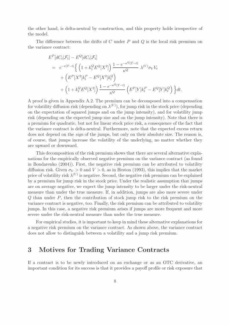
The difference between the drifts of C under P and Q is the local risk premium onthe variance contract:

EP [dCt|Ft] − EQ[dCt|Ft]

= e−r(T−t){(

1 + kQ1 EQ[X2]

) 1 − e−κQ(T−t)

κQλ(V )σV Vt

+(EP [X2]kP

t − EQ[X2]kQt

)

+(1 + k

Q1 EQ[X2]

) 1 − e−κQ(T−t)

κQ

(EP [Y ]kP

t − EQ[Y ]kQt

)}dt.

A proof is given in Appendix A.2. The premium can be decomposed into a compensationfor volatility diffusion risk (depending on λ(V )), for jump risk in the stock price (dependingon the expectation of squared jumps and on the jump intensity), and for volatility jumprisk (depending on the expected jump size and on the jump intensity). Note that there isa premium for quadratic, but not for linear stock price risk, a consequence of the fact thatthe variance contract is delta-neutral. Furthermore, note that the expected excess returndoes not depend on the sign of the jumps, but only on their absolute size. The reason is,of course, that jumps increase the volatility of the underlying, no matter whether theyare upward or downward.

This decomposition of the risk premium shows that there are several alternative expla-nations for the empirically observed negative premium on the variance contract (as foundin Bondarenko (2004)). First, the negative risk premium can be attributed to volatilitydiffusion risk. Given σV > 0 and V > 0, as in Heston (1993), this implies that the marketprice of volatility risk λ(V ) is negative. Second, the negative risk premium can be explainedby a premium for jump risk in the stock price. Under the realistic assumption that jumpsare on average negative, we expect the jump intensity to be larger under the risk-neutralmeasure than under the true measure. If, in addition, jumps are also more severe underQ than under P , then the contribution of stock jump risk to the risk premium on thevariance contract is negative, too. Finally, the risk premium can be attributed to volatilityjumps. In this case, a negative risk premium arises if jumps are more frequent and moresevere under the risk-neutral measure than under the true measure.

For empirical studies, it is important to keep in mind these alternative explanations fora negative risk premium on the variance contract. As shown above, the variance contractdoes not allow to distinguish between a volatility and a jump risk premium.

3 Motives for Trading Variance Contracts

If a contract is to be newly introduced on an exchange or as an OTC derivative, animportant condition for its success is that it provides a payoff profile or risk exposure that

8

investors actually want to trade. For the variance contract the question is thus whetherthe investor is interested in an exposure to the second moment of stock returns.

As the theoretical basis for our analyses we rely on the work of Liu and Pan (2003)and the extension by Branger, Schlag, and Schneider (2005b). The latter paper analyzesthe portfolio planning problem of an investor with a CRRA utility function in a modelwhich is characterized by SV and jumps in both the stock price and in volatility. Tosimplify the analysis, we assume that jumps occur simultaneously and that their sizeis deterministic. The dynamics of the stock price and the SV component are given inEquations (1) and (2), again with the additional assumptions that the jump sizes aredeterministic, i.e. eX − 1 ≡ µX and Y ≡ µY . Furthermore, we assume that the jumpintensities are proportional to V , i.e. kP

0 = kQ0 = 0. The risk premium for one unit of

dW(S)t is given by ηB1

√Vt, the compensation for dW

(V )t is ηB2

√Vt. The market prices of

risk introduced in Section 2.1 are then given by

λ(S) = ηB1

λ(V ) = ρ ηB1 +√

1 − ρ2ηB2.

In the above setup the market is complete with two additional instruments besides thestock and the money market account. Branger, Schlag, and Schneider (2005b) solve theportfolio planning problem for an investor with constant relative risk aversion (powerutility). The dynamics of wealth W are

dWt = Wt

{rdt + θ

(S)t

(√VtdW

(S)t + ηVtdt

)+ θ

(V )t

(√VtdW

(V )t + ξVtdt

)

+ θ(N)t

[dNt − kP

1 Vt dt +(kP

1 − kQ1

)Vt dt

]}

where the exposures to the three fundamental sources of risk√

VtW(S),

√VtW

(V ), and N

are used instead of the investments in the different assets. In a complete market, thereexists a dynamic trading strategy for every possible exposure.

As part of the solution the optimal exposure is determined as

θ∗St =ηB1

γ+ ρσV H(τ)

θ∗Vt =ηB2

γ+√

1 − ρ2σV H(τ)

θ∗Nt =

[(kP

1

kQ1

)1/γ

− 1

]+

(kP

1

kQ1

)1/γ [eH(τ)µY − 1

], 1 + θ∗Nt ≥ 0.

with γ as the investor’s coefficient of risk aversion and τ as the remaining investmenthorizon. The function H solves the ordinary differential equation

H ′(τ) = a + b exp{µY H(τ)} + c H(τ) + d H2(τ) (5)

9

with the boundary condition H(0) = 0 and

a =1 − γ

2γ2

[(ηB1)2 + (ηB2)2

]+

1 − γ

γk

Q1 − 1

γkP

1

b = kQ1

(kP

1

kQ1

)1/γ

c = −(κP + µY kP

1

)+

1 − γ

γσV

(ρηB1 +

√1 − ρ2ηB2

)

d =1

2σ2

V .

The optimal exposure can be decomposed into a speculative demand (first summand)and a hedging demand (second summand). For the diffusion components the speculativedemand depends on the ratio of the risk premium to the coefficient of risk aversion,while the hedging demand is mainly driven by the correlation between stock returns andvolatility changes. For the jump component, there is also a speculative demand, and thehedging demand vanishes only in case µY = 0, that is when jumps have no impact onthe state variable V . For a more detailed discussion of the optimal demand, the reader isreferred to Liu and Pan (2003) and Branger, Schlag, and Schneider (2005b).

If only the stock and the money market account are traded, the investor cannotachieve an exposure to W (V ), and the exposures to W (S) and N are fixed at the relationgiven by the stock price process. To obtain his optimal exposure, the investor thus hasto use derivatives, which shows that there is a need for contracts providing exposureto the individual risk factors. Depending on the level of risk aversion and the amountof the risk premia, the sign of the optimal exposure can vary, i.e. both long and shortpositions in the risk factors can basically be optimal. While this analysis is performed ina partial equilibrium model, Branger, Schlag, and Schneider (2005a) show that there isalso a trading demand for variance risk in a general equilibrium setup with heterogeneousagents.

4 Replication Strategies

As mentioned in the introduction, a new derivative will only be introduced if it cannot beeasily replicated (at least not by a sufficiently large group of investors) by claims that arealready traded in the market. In this paper, we focus on the degree of sensitivity to modelrisk as a key parameter in measuring the economic value of a newly introduced derivativecontract. Even if the contract was basically replicable in a scenario with perfect knowledgeabout the true data-generating process, the hedge errors occurring due to a mis-specifiedhedge model may nevertheless be substantial. In this case investors might prefer tradingthe variance contract itself to the supposedly replicating strategy which turns out to bemore risky. However, this argument not only holds for the variance contract, but also forother derivatives. Which contract should ultimately be introduced depends on the amountof model risk exposure.

10

Before we analyze the impact of model risk on dynamic replicating strategies, we takea closer look at semi-static hedging strategies for the variance contract. If the stock pricefollows a diffusion process, interest rates are deterministic, and if a continuum of optionswith strike prices from zero to infinity are available for trading, then there is a perfectand model-independent hedge for the variance contract. This hedge, however, fails if thestock price can jump.

4.1 Semi-Static Replication

Since the paper of Breeden and Litzenberger (1978), it is well known that a Europeanpath-independent claim can be replicated by a static portfolio of a continuum of Europeancall options with the same time to maturity. Furthermore, its decomposition is model-independent and consequently not exposed to model risk.

The principle of static hedging cannot be applied directly to variance contracts, sincetheir payoff is highly path-dependent. In a diffusion model, however, it can be shown thatthe payoff of the variance contract is equal to the payoff from a log-contract (for which astatic replication is possible) and a simple dynamic strategy in the stock, c.f. Neuberger(1994). This hedge is perfect for diffusion models, but it fails if the stock price can jumpor if interest rates are stochastic. In the following, we will concentrate on the impact ofjumps, but retain the assumption of deterministic interest rates.

In our general model introduced in Section 2.1, it holds that

d lnSt −dSt

St−

= −0.5Vtdt +[Xt −

(eX−t − 1

)]dNt.

We can thus conclude that

∫ T

0

Vtdt +

∫ T

0

X2t dNt = −2(ln ST − ln S0) + 2

∫ T

0

dSt

St−

+ 2

∫ T

0

[Xt + 0.5X2

t −(eX−t − 1

)]dNt,

which is linked to the ’static replicating strategy’ for the variance contract in case oflog-returns. For discrete returns, we get

∫ T

0

Vtdt +

∫ T

0

(eXt − 1

)2dNt = −2(ln ST − ln S0) + 2

∫ T

0

dSt

St−

+ 2

∫ T

0

[Xt + 0.5

(eXt − 1

)2 −(eX−t − 1

)]dNt

The first term on the right hand side is in both cases related to the log-contract. It canbe replicated by a static position in a continuum of European options with maturity in T

and by a position in the money market account. The second term on the right hand sidecan be replicated by a dynamic trading strategy in the stock or in the futures contract,

11

where the number of stocks (futures) depends on the current stock (futures) price and onthe interest rate.

If there are no jumps, the third term is zero in both cases, and the strategy justdescribed is a perfect hedge for the variance contract. In case of a jump, however, thisterm deviates from zero and causes the replication strategy to fail. Figure 1 shows thisreplication error as a function of the jump size eXt − 1 in the stock price. The left paneldescribes the error if the realized variance is based on log returns, and the right panelgives the error if discrete returns are used. The upper row shows that the error is quitelow for jumps below 10%, but increases sharply for more extreme jumps. To get an ideaof the severity of the problem, we compare the hedging error due to jumps to severalbenchmarks. First, the final payoff due to diffusion variance is on average equal to θP τ

where τ is the time to maturity. For θP = 0.02, an error of 0.002 is equal to the payoff dueto diffusion variance accumulated over 0.1 years. A jump contributes X2

t or (eXt − 1)2 tothe final payoff. As shown in the middle row, the hedging error is equal to approx. 2-8%of this payoff. Second, we can take the price of the contract as a benchmark. For a timeto maturity of one month, the error in case of a jump of 20% is equal to up to 5% (incase of log returns) or 20% (in case of discrete returns) of the price of the contract, as canbe seen from the bottom row. While the error is thus quite small compared to the totalpayoff in case of a jump (and thus has a small contribution to the price, as also shown inJiang and Tiang (2005)), it is quite large compared to the initial price of the contract.

Bondarenko (2004) discusses a modification of the payoff function which is adjustedin such a way that the hedge described above is perfect even in case of jumps (but not incase of stochastic interest rates). For all other specifications of the contract, hedging thejump part of realized variance is still a problem. And in most cases it will be the payoffwhich is given first (and for which a hedging strategy has to be found) rather than theother way around.

4.2 Basic Setup for Dynamic Hedging Strategies

In the following sections we analyze the performance of dynamic hedging strategies for thevariance contract under various types of model risk. We furthermore analyze the hedgingerrors for a deep OTM put option with a strike price equal to 85% of the current stockprice. This option is one example for a contract that competes with the variance contractfor introduction. It also completes the market in the sense that it enlarges the set ofstatically replicable payoffs. From an economic point of view, it provides crash protectionand would thus be of interest to investors. Our results show that the variance contractis indeed significantly exposed to model risk, and that it has a higher exposure than theput. Thus, if there is a need for an enlargement of the set of traded contracts, the variancecontract offers a more significant improvement than just another put option.

The objective is to replicate some claim H , and in the following this H will eitherbe an OTM-put or the variance contract. St is the current stock price, the price of theclaim to be hedged is Ht = h(t, St, Vt, . . .), and C

(i)t = c(i)(t, St, Vt, . . .) stands for the price

12

of the i-th hedge instrument written as a function of the state variables. The number ofshares in the hedge portfolio at time t is denoted by φ

(S)t , and the number of units of the

hedge instrument i at time t is φ(i)t for i = 1, . . . , n. If there is only one instrument we

denote its price by C and the associated number of units by φ(C)t . Except for time, partial

derivatives are denoted by subscripts.

Besides the true model describing the dynamics of the stock price and the state vari-ables, there is a model assumed by the investor (hedge model). Whenever the calculationof the prices or the portfolio composition is done in this hedge model, we denote thevariables by a tilde. For example, φ̃(S) is the number of shares of the stock in the hedgeportfolio as calculated in the hedge model.

The hedge portfolio is chosen in such a way that its sensitivities (as calculated in thehedge model) with respect to the different risk factors are equal to those of the claimto be hedged. We make the assumption of market completeness which will be discussedbelow. For the diffusion risk of the stock this means

φ̃(S)1 + φ̃(1)c̃(1)s + . . . + φ̃(n)c̃(n)

s = h̃s, (6)

while for the state variable variance V we must have that

φ̃(1)c̃(1)v + . . . + φ̃(n)c̃(n)

v = h̃v. (7)

The analogous condition for jump risk is

φ̃(S)∆S̃ + φ̃(1)∆c̃(1) + . . . + φ̃(n)∆c̃(n) = ∆h̃, (8)

where ∆h and ∆c(i) denote the change in the prices of the claim and the i-th hedgeinstrument, respectively. By subtracting Equation (6) (multiplied by ∆S̃) from Equation(8), this condition can also be rewritten as

φ̃(1)(∆c̃(1) − c̃(1)

s ∆S̃)

+ . . . + φ̃(n)(∆c̃(n) − c̃(n)

s ∆S̃)

=(∆h̃ − h̃s∆S̃

). (9)

The terms in brackets denote the additional jump risk of the derivatives that remainsafter delta-hedging with the stock. Of course, we would have a condition like this for anypossible jump size (or for any jump size we decide to hedge).

The equations above are given for the hedge model. The same conditions determinethe correct replicating portfolio in the true model. However, note that the number of riskfactors and the type of risk factors need not be the same in the true and in the hedgemodel.

As the data-generating process, we consider simple extensions of the Black-Scholesmodel. To be specific, we work with the jump-diffusion model developed by Merton (1976),the SV model of Heston (1993), and the general model suggested by Bakshi, Cao, andChen (1997) (assuming a constant interest rate), which are the most prominent modelsthat include stochastic volatility and/or jump risk. The analysis would only become moreinvolved in more complicated models.

13

As a hedge model, we use the SV model of Heston (1993) and the jump-diffusionmodel developed by Merton (1976) where we make the simplifying assumption of a deter-ministic jump size. The hedge model is calibrated to the prices of certain options whichare calculated in the true model. For our examples, we rely on European options withmoneyness (strike-to-spot ratio) of 0.95, 1, 1.05, and (in case of the SV model) also 0.9,and with a time to maturity of six months which is equal to the time to maturity ofthe claim to be hedged. We allow for a non-perfect fit of the hedge model to the data,i.e. a hedge model is considered acceptable as long as the maximum deviation of modelprices from given market prices is not too large. The investor might consider the hedgemodel as a simple approximation to the much more complicated true model. Furthermore,real world market frictions like bid-ask spreads could make it almost impossible to inferthe exact model and/or the exact parameters anyway, as shown by Dennis and Mayhew(2004). Given the cross section of noisy prices, the investor thus cannot avoid parameterrisk and model risk.

The choice of the two hedge models is motivated by several criteria. Our main pointis to analyze the impact of model mis-specification on the hedging error. To focus on thisquestion, we make several simplifying assumptions. First, we assume that the hedge modelis complete. In an incomplete hedge model, we would have to decide on a hedge criterionlike the variance of the hedging error or the shortfall probability. This would introducean additional dependence of the hedging error on this choice without contributing to themain problem analyzed in the study. Second, we assume that there are just enough hedgeinstruments to achieve market completeness. Otherwise, the replicating strategy would nolonger be unique, and we would have to decide on some additional criterion to choose oneof these strategies. Again, this would introduce an additional dependence of the hedgingerror on this choice and would distract from the main focus of the study. And finally, weassume that one additional option besides the stock and the money market account isenough to complete the market. Thus, all hedging strategies we consider in the followinguse the same number of instruments, which again facilitates their comparison.

The value of the hedge portfolio at time t is denoted by Πt. We assume that the hedgeportfolio is self-financing, i.e. any proceeds are invested into the money market account,earning the constant risk-free rate r. At time t the hedging error is Dt = Ht − Πt. Tocompare the hedge based on the hedge model to the perfect hedge, we calculate the localhedging error, i.e. we derive the stochastic differential equation (SDE) for the hedgingerror. As will be shown in more detail below, the general structure of the hedging erroris given by

dDt = . . . dt +{hs − h̃s − φ̃

(C)t (cs − c̃s)

}St

(√VtdW

(S)t + λ(S)Vtdt

)

+{hv − h̃v − φ̃

(C)t (cv − c̃v)

}σV

√Vt

(ρdW

(S)t +

√1 − ρ2dW

(V )t + λ(V )

√Vtdt

)

+{(

∆h − h̃s∆S)−(∆h̃ − h̃s∆S̃

)

−φ̃(C)t

[(∆c − h̃s∆S

)−(∆c̃ − c̃s∆S̃

)]}dNt. (10)

If in the true model, volatility is not stochastic, the term in the second line is set equal

14

to zero, and if there is no jump risk, the term in the third line is set equal to zero.Analogously, the sensitivities are set equal to zero if the corresponding risk factor doesnot exist in the true model or in the hedge model, respectively.

The hedging error from Equation (10) can be decomposed into errors due to stockdiffusion risk, volatility diffusion risk, and jump risk. Each of the three summands isequal to the remaining exposure to this risk factor, multiplied with the risk factor and itscompensation. Consider the impact of volatility diffusion risk. The remaining exposureof the hedge portfolio – which is zero in case of a perfect hedge – can be explained bytwo kinds of errors. First, the sensitivities of the claim to be hedged are calculated in thehedge model and therefore deviate from the true partials (hv− h̃v). Second, the sensitivityof the hedge instrument C with respect to volatility is also calculated in the wrong model,so that the wrong number of units of the hedge instruments is employed to eliminate agiven volatility risk exposure (cv − c̃v). The impact of stock diffusion risk and of jump riskis similar.

Model risk does not necessarily imply that there is a hedging error. It may also happenthat the errors in the calculation of the exposure to be hedged are offset by the errors inthe calculation of the exposure of the instrument used for hedging. If this is the case, thehedge is robust with respect to model risk, and one objective in the following will be tosearch for such a robust hedge. Intuitively, the conjecture is that the hedge will be themore robust the more similar the claim to be hedged and the hedge instrument are. Forthe variance contract which is exposed to stochastic volatility and to jump risk, there aretwo natural candidates for a robust hedge. The first is an ATM straddle (or ATM option)which is often considered as a an instrument that is mainly exposed to volatility risk. Thesecond candidate is an OTM put, which mainly provides exposure to downward jumps inthe stock price.

To assess the impact of model risk, the next subsections contain an analysis of thehedging error from Equation (10) over the a short time interval of length dt. We assumethat there is a one-standard deviation shock in each of the diffusion terms, i.e. we assumethat the stock price changes by

√VtStdt. In case of stochastic volatility, the same is done

for the stochastic volatility component, which is shocked by σV

√Vtdt. For this infinitesimal

change, the hedging error follows from the SDE. It is then annualized by dividing by dt

and expressed as a fraction of the current price of the claim to be hedged. For the jumpcomponent, we consider the hedging error if there is a jump, and again express it as afraction of the current price of the claim.

4.3 Parameter Risk

We start our analysis by considering the case of parameter risk. Here, the assumption isthat the investor uses the correct model (e.g., Heston (1993) or Merton (1976)), but withan incorrect parametrization. Even if an investor knew the true model type with certainty,he or she would have to estimate the parameters and thus could not avoid estimation risk(parameter risk).

15

4.3.1 Stochastic Volatility Model

In the model suggested by Heston (1993), the local variance of the stock follows a mean-reverting square-root process. The dynamics under the true measure are given by

dSt = (r + λSVt) dt +√

VtStdW St

dVt = κP (θP − Vt) dt + σV

√Vt

(ρdW S

t +√

1 − ρ2dW Vt

).

We consider the hedging error under parameter risk for a hedge portfolio consisting of thestock, the hedge instrument and the money market account. The SDE for the hedgingerror D is stated in

Proposition 1 (SV under Parameter Risk)

dDt = (Ht − Πt)rdt +{hs − h̃s − φ̃

(C)t (cs − c̃s)

}(dSt − rStdt)

+{

hv − h̃v − φ̃(C)t (cv − c̃v)

}(dVt − κQ(θQ − Vt)dt

), (11)

where the number of units of the hedge instrument is given by

φ̃(C)t =

h̃v

c̃v.

A proof can be found in Appendix A.3.

The first term in brackets on the right hand side of Equation (11) is the interestearned on the hedging error accumulated up to time t. It is not relevant for our analysis,since it does not depend on the choice of the hedge portfolio at time t. We rather focuson those components of the local hedging error that could still be avoided if we knew thecorrect model, i.e. on the second and third term.

Despite parameter risk there is still a chance for the hedge to produce a zero error.When the errors in the sensitivities of the claim and the hedge instrument exactly offseteach other, i.e. when

hs − h̃s − φ̃(C)t (cs − c̃s) = 0

andhv − h̃v − φ̃

(C)t (cv − c̃v) = 0,

the hedging error vanishes. These robustness conditions trivially hold in the true model. Ifthe hedge model deviates from the true model, our conjecture is that the more similar theclaim to be hedged is to the hedge instrument, the more similar the partial derivatives andalso the associated errors will be, and thus the lower the replication error. This impliesthat when we use options as our hedge instruments, other options with a different strikeshould be easier to hedge than the variance contract. Furthermore, the hedge for a putshould be the better the smaller the difference of the strike prices between the put andthe option used in the hedge.

16

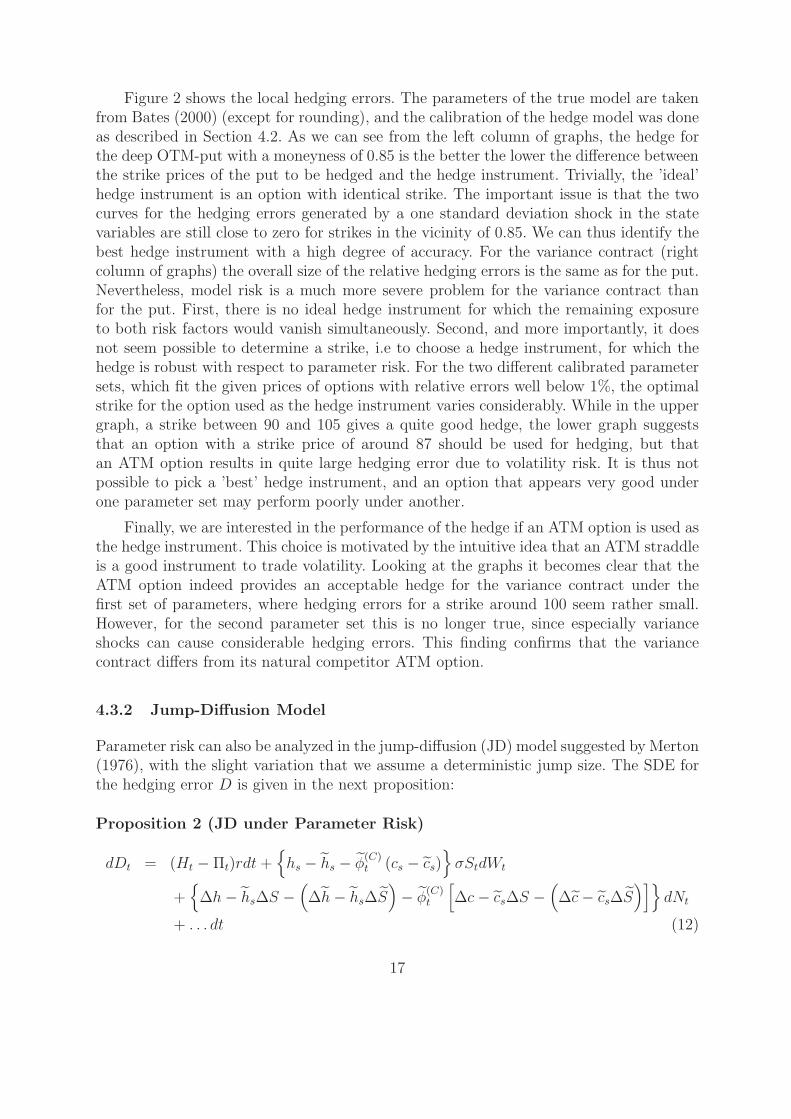
Figure 2 shows the local hedging errors. The parameters of the true model are takenfrom Bates (2000) (except for rounding), and the calibration of the hedge model was doneas described in Section 4.2. As we can see from the left column of graphs, the hedge forthe deep OTM-put with a moneyness of 0.85 is the better the lower the difference betweenthe strike prices of the put to be hedged and the hedge instrument. Trivially, the ’ideal’hedge instrument is an option with identical strike. The important issue is that the twocurves for the hedging errors generated by a one standard deviation shock in the statevariables are still close to zero for strikes in the vicinity of 0.85. We can thus identify thebest hedge instrument with a high degree of accuracy. For the variance contract (rightcolumn of graphs) the overall size of the relative hedging errors is the same as for the put.Nevertheless, model risk is a much more severe problem for the variance contract thanfor the put. First, there is no ideal hedge instrument for which the remaining exposureto both risk factors would vanish simultaneously. Second, and more importantly, it doesnot seem possible to determine a strike, i.e to choose a hedge instrument, for which thehedge is robust with respect to parameter risk. For the two different calibrated parametersets, which fit the given prices of options with relative errors well below 1%, the optimalstrike for the option used as the hedge instrument varies considerably. While in the uppergraph, a strike between 90 and 105 gives a quite good hedge, the lower graph suggeststhat an option with a strike price of around 87 should be used for hedging, but thatan ATM option results in quite large hedging error due to volatility risk. It is thus notpossible to pick a ’best’ hedge instrument, and an option that appears very good underone parameter set may perform poorly under another.

Finally, we are interested in the performance of the hedge if an ATM option is used asthe hedge instrument. This choice is motivated by the intuitive idea that an ATM straddleis a good instrument to trade volatility. Looking at the graphs it becomes clear that theATM option indeed provides an acceptable hedge for the variance contract under thefirst set of parameters, where hedging errors for a strike around 100 seem rather small.However, for the second parameter set this is no longer true, since especially varianceshocks can cause considerable hedging errors. This finding confirms that the variancecontract differs from its natural competitor ATM option.

4.3.2 Jump-Diffusion Model

Parameter risk can also be analyzed in the jump-diffusion (JD) model suggested by Merton(1976), with the slight variation that we assume a deterministic jump size. The SDE forthe hedging error D is given in the next proposition:

Proposition 2 (JD under Parameter Risk)


(C)t (cs − c̃s)

}σStdWt

+{

∆h − h̃s∆S −(∆h̃ − h̃s∆S̃

)− φ̃

(C)t

[∆c − c̃s∆S −

(∆c̃ − c̃s∆S̃

)]}dNt

+ . . . dt (12)

17

where the omitted dt-terms capture the risk premia for the risk remaining in the portfolio

and where the number of claims is given by

φ̃(C)t =

∆h̃ − h̃s∆S̃

∆c̃ − c̃s∆S̃.

The proof can be found in Appendix A.4. Note that the jump size ∆S in the true model canwell be different from the assumed jump size ∆S̃ in the hedge model. The interpretationof the SDE for the hedging error is similar to the case of the SV model discussed in theprevious subsection. There are again robustness conditions under which the hedge willproduce a zero error, despite the fact that incorrect parameters are used.

Figure 3 shows the relative hedging error for a local one standard deviation changeσStdt in the stock price, and for the case when a jump occurs, i.e. for a change of thestock price by ∆S = µXSt−. The results are in general similar to those found for the SVmodel. For the deep OTM put the hedge is the better the smaller the difference betweenits strike and the strike of the option used as a hedge instrument. The variance contractis again more difficult to hedge than the put. As in the SV case there is no choice ofthe hedge instrument for which the hedge would be insensitive to model risk. The ATMoption, which is considered as a natural instrument to trade volatility risk, is again notthe ideal hedge instrument. Furthermore, an OTM put which is often considered as areliable hedge against jump risk does not perform well either.

The pictures also show that jump risk is in general more difficult to hedge thanstock price risk or volatility risk. Note that this cannot be explained by a generic modelincompleteness due to jumps or by the fact that a local delta hedge could possibly notcontrol for large changes in the stock price due to a jump. Our model is complete byconstruction, so that a perfect hedge is basically feasible. The hedging errors are onlycaused by parameter risk, and the results show that especially the estimation of the jumpsize is a quite severe problem.

4.4 Mis-Specification of Risk Factors

Model mis-specification describes a situation where the wrong model is used for the hedge,and not just a model of the correct type with incorrect parameter values. In this sectionwe focus on the case of a mis-specification of risk factors. The investor assumes the JDmodel, although the true model is SV, and vice versa. In Section 4.5 we will then analyzethe case of omitted risk factors, where the hedge model is a restricted version of the truemodel. Intuitively, we would expect that model mis-specification has much more severeconsequences for the general structure of hedging errors than an incorrect parametrization.

4.4.1 Stochastic Volatility Model

We start with the case when SV is the true model, but JD is used as the hedge model.Both models can, for example, produce a downward sloping smile. The investor might not

18

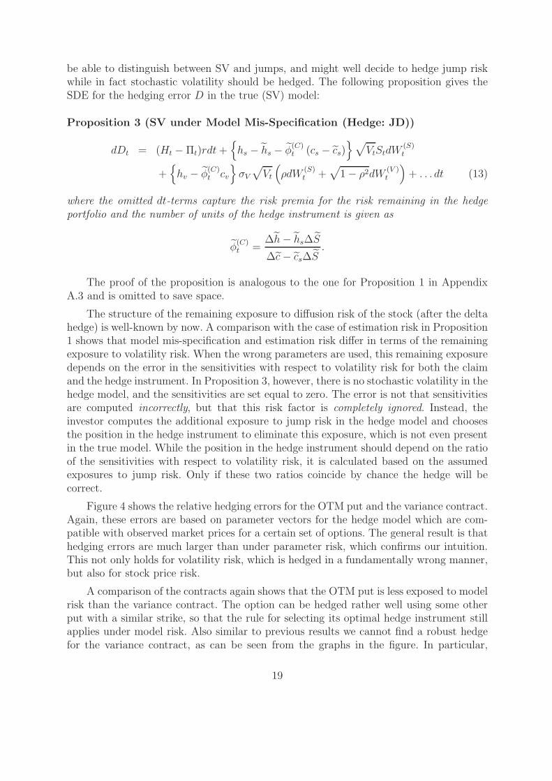
be able to distinguish between SV and jumps, and might well decide to hedge jump riskwhile in fact stochastic volatility should be hedged. The following proposition gives theSDE for the hedging error D in the true (SV) model:

Proposition 3 (SV under Model Mis-Specification (Hedge: JD))


(C)t (cs − c̃s)

}√VtStdW

(S)t

+{

hv − φ̃(C)t cv

}σV

√Vt

(ρdW

(S)t +

√1 − ρ2dW

(V )t

)+ . . . dt (13)

where the omitted dt-terms capture the risk premia for the risk remaining in the hedge

portfolio and the number of units of the hedge instrument is given as

φ̃(C)t =

∆h̃ − h̃s∆S̃

∆c̃ − c̃s∆S̃.

The proof of the proposition is analogous to the one for Proposition 1 in AppendixA.3 and is omitted to save space.

The structure of the remaining exposure to diffusion risk of the stock (after the deltahedge) is well-known by now. A comparison with the case of estimation risk in Proposition1 shows that model mis-specification and estimation risk differ in terms of the remainingexposure to volatility risk. When the wrong parameters are used, this remaining exposuredepends on the error in the sensitivities with respect to volatility risk for both the claimand the hedge instrument. In Proposition 3, however, there is no stochastic volatility in thehedge model, and the sensitivities are set equal to zero. The error is not that sensitivitiesare computed incorrectly, but that this risk factor is completely ignored. Instead, theinvestor computes the additional exposure to jump risk in the hedge model and choosesthe position in the hedge instrument to eliminate this exposure, which is not even presentin the true model. While the position in the hedge instrument should depend on the ratioof the sensitivities with respect to volatility risk, it is calculated based on the assumedexposures to jump risk. Only if these two ratios coincide by chance the hedge will becorrect.

Figure 4 shows the relative hedging errors for the OTM put and the variance contract.Again, these errors are based on parameter vectors for the hedge model which are com-patible with observed market prices for a certain set of options. The general result is thathedging errors are much larger than under parameter risk, which confirms our intuition.This not only holds for volatility risk, which is hedged in a fundamentally wrong manner,but also for stock price risk.

A comparison of the contracts again shows that the OTM put is less exposed to modelrisk than the variance contract. The option can be hedged rather well using some otherput with a similar strike, so that the rule for selecting its optimal hedge instrument stillapplies under model risk. Also similar to previous results we cannot find a robust hedgefor the variance contract, as can be seen from the graphs in the figure. In particular,

19

an OTM put with strike-to-spot ratio of 0.95, which might be recommended as a hedgeagainst downward jump risk, performs quite well for the second parameter set, but ratherpoorly for the first. The ATM option, on the other hand, provides a pretty good hedgeunder the first calibrated parameter set, but not under the second.

4.4.2 Jump-Diffusion Model

Now the situation will be reversed, and JD with deterministic jump size will be the truemodel, while SV will be used as the hedge model. The SDE for the hedging error D underthe true model is the content of the next proposition.

Proposition 4 (JD under Model Mis-Specification (Hedge: SV))


(C)t (cs − c̃s)

}σStdWt

+{

∆h − h̃s∆S − φ̃(C)t (∆c − c̃s∆S)

}dNt + . . . dt, (14)


portfolio and where the number of claims is determined as

φ̃(C)t =

h̃v

c̃v

.

The proof of this proposition is analogous to that for Proposition 2 and is omitted tosave space.

The structure of the remaining exposure to diffusion risk of the stock has alreadybeen discussed extensively. The remaining exposure to the jump risk of the stock is muchmore interesting. Like for the SV model the remaining exposure under model risk inEquation (14) is quite different from its counterpart under parameter risk in Equation (12).Under parameter risk the hedging error depends on the difference between the exposures tojump risk in the true and in the hedge model for both the claim and the hedge instrument.Here the hedge model does not even contain a jump component, so that the exposure withrespect to this risk factor is basically set equal to zero. Instead the investor aims at hedgingvolatility risk not present in the true model. Again the hedge is only correct, if, by chance,the ratio of exposure to volatility in the hedge model is equal to the ratio of the exposuresto additional jump risk in the true model.

Figure 5 shows the familiar result that the hedging error for the OTM put can bekept small by choosing a put with a similar strike price as the hedge instrument. Again,there is no ideal hedge instrument for the variance contract, which further underlines thatthis derivative asset is harder to replicate in a world with model risk than the simple put.Especially the impact of a jump is quite pronounced.

20

4.5 Model Risk: Missing Risk Factors

Another variant of model mis-specification is that the hedge model is less general thanthe true model, i.e. some of the risk factors included in the true model are omitted fromthe hedge model. For example, the true model could contain a multi-factor specificationfor stochastic volatility, as in Bates (2000), whereas the hedge model is a one-factor modellike the one suggested by Heston (1993). It could also be the case that the general modeldeveloped by Bakshi, Cao, and Chen (1997) generates the data, while the hedge model isa restricted variant, like Heston (1993) or Merton (1976), where either stochastic jumps orstochastic volatility are missing. We will discuss two cases of omitted risk factors, wherethe true model is always given by a version of Bakshi, Cao, and Chen (1997) with adeterministic jump size for the stock. First, the jump component is omitted in the hedgemodel, and second, we analyze the consequences of leaving out the stochastic volatilitypart instead.

Again, this kind of model risk is quite likely to strike when a hedge is implemented.The true model will be able to explain many observable phenomena correctly, and it willusually be quite sophisticated with a large number of state variables and parameters. Evenif we can find the correct type of model its parameters will be difficult to identify. Wethus assume that the investor uses a simpler model which fits the data ’sufficiently’ well.Once such a simpler model has been found, it would be hard to justify a more complexapproach.

4.5.1 Omitted Jump Component

We start our analysis with the case where the jump component is missing from the hedgemodel. As usual, we first derive the dynamics of the hedging error in the true model:

Proposition 5 (BCC Model: Hedge under Model Mis-Specification (SV))


(C)t (cs − c̃s)

}√VtdW

(S)t

+{

hv − h̃v − φ̃(C)t (cv − c̃v)

}σV

√Vt

(ρdW

(S)t +

√1 − ρ2dW

(V )t

)

+{

∆h − h̃s∆S − φ̃(C)t (∆c − c̃s∆S)

}dNt + . . . dt (15)


portfolio and where the number of claims is

φ̃(C)t =

h̃v

c̃v.

The proof is similar to that for Proposition 1 in Appendix A.3.

The remaining exposure to stock price risk and to volatility risk has the same structureas in the case of parameter risk in the SV model discussed in Proposition 1. The most

21

interesting part of Equation (15) is the one that relates to the jump risk exposure leftin the hedge portfolio. As in Proposition 4, jump risk is missing from the hedge modeland has been incorrectly interpreted as stochastic volatility. However, the investor nowmakes a second mistake. There are fewer risk factors in the hedge model than in the truemodel, so that there are not enough instruments in the hedge portfolio from the start, andthe bad hedge for jump risk is unavoidable. Jump risk could now be eliminated only bychance, if the ratio of the additional exposure to jump risk for H and the hedge instrumentcoincides with the analogous ratio with respect to volatility risk.

Figure 6 shows the result of the analysis of the local relative hedging error. For theput the results are the same as in the cases studied before. One additional point to noteis that the sensitivity of the hedge to shocks in the risk factors looks rather large evenfor this simple instrument, and that, depending on the model, volatility risk (present inthe hedge model) may be as hard to hedge as jump risk (missing from the hedge model).Furthermore, looking at the left column of graphs we can see that the quality of the hedgedeteriorates especially when the stock price has jumped. For the variance contract there isagain no optimal hedge instrument which provides robustness with respect to model risk.Additionally, we have to keep in mind that the hedge model (Heston (1993)) is exposedto a kind of parameter risk. As discussed in Subsection 4.4.1, there may be more thanone parametrization which fits the given prices, and these two problems add up in thehedging error.

4.5.2 Omitted Stochastic Volatility

As the last case we analyze the hedging error when the hedge model only contains a jumpcomponent, but no stochastic volatility.

Proposition 6 (BCC Model: Hedge under Model Mis-Specification (JD))


(C)t (cs − c̃s)

}√VtStdW

(S)t

+{hv − φ̃

(C)t cv

}σV

√Vt

(ρdW

(S)t +

√1 − ρ2dW

(V )t

)

+{

∆h − h̃s∆S −(∆h̃ − h̃s∆S̃

)− φ̃

(C)t

[(∆c − c̃s∆S) −

(∆c̃ − c̃s∆S̃

)]}dNt

+ . . . dt (16)


portfolio and where the number of claims is

φ̃(C)t =

∆h̃ − h̃s∆S̃

∆c̃ − c̃s∆S̃.

The proof is analogous to that for Proposition 2 in Appendix A.4.

The interpretation of Equation (16) is very similar to those for the previous proposi-tions. The structure of the remaining exposure to jump risk and to stock diffusion risk is

22

identical to the case of parameter risk which has been given in Proposition 2. For volatilityrisk the structure of the remaining exposure had already been discussed in Proposition4, where stochastic volatility was also not included in the hedge model. However, in thecase where stochastic volatility had incorrectly been interpreted as jump risk, there wouldat least have been the chance to construct the correct hedge, since the right set of in-struments was available. Here, this is basically impossible, since there are not enoughinstruments in the hedge portfolio to achieve completeness. Volatility risk is thus onlyhedged by chance.

Figure 7 compares the hedging errors for a deep OTM put and the variance contract.It shows that a hedge for the variance contract based on a mis-specified model can generatesubstantial hedging errors and that there is no robust choice of hedge instruments. Forexample, the upper graph in the right column seems to suggest that including a put witha strike price of roughly 106 generates relatively small errors. However, the lower graphshows that this does not hold in general. The hedging errors for this hedge instrumentcan be rather large under a different parameter scenario, which nevertheless prices theset of given contracts with acceptable precision. In particular, the remaining exposure tostochastic volatility is rather large.

5 Conclusion

Variance contracts are innovative derivative assets. They provide exposure to the variationrisk of a stock, that is to stochastic volatility and jumps. Empirically there is evidence fora negative risk premium on the variance contract, which is usually explained by the well-documented negative market price of risk for stochastic volatility. A second explanation,however, is that stock price jumps and/or volatility jumps can be perceived to be moresevere and more frequent under the risk-neutral than under the physical measure. Thevariance contract does not allow to distinguish between the risk factors volatility andjumps.

The main motivation for trading the variance contract comes from the optimal port-folio decision of investors. The investor wants an instrument providing him with exposureto variation risk of the stock, which has a high payoff if the diffusion variance has increasedor if there have been jumps in the stock price. A formal motivation can be derived fromthe literature on portfolio planning, which shows that investors can have a demand forportfolios providing a hedge against fluctuations in the state variables. Given this (mainlyspeculative) demand, the question is then why investors would prefer the variance contractto a replicating strategy using standard options.

In our opinion the main economic motivation for the introduction of variance contractsis that the variance contract is ’better’ than its replicating strategy and that it provides amore significant improvement relative to its replicating strategy than a standard option.This implies that there is a stronger motivation to introduce the variance contract thanthe option. There are at least two arguments for the superiority of the variance contractcompared to a replication strategy. First, the semi-static hedging strategy fails if there

23

are jumps in the stock price. Second, every dynamic replication strategy has to be basedon some assumed model, and a hedging error will result if the hedge model is not equalto the true model.

In the paper, we consider the cases of parameter uncertainty and of mis-specified andomitted risk factors. Under all of these scenarios we derive analytical expressions for thelocal hedging errors. A graphical analysis shows that the hedging error for the variancecontract is in general slightly larger than that for a deep OTM put, which was chosenas the benchmark asset and as an alternative candidate for the new derivative contractto be introduced. However, the variance contract is exposed to model risk to a muchhigher degree. For the put, the hedge is the more robust against model risk the smallerthe difference between its strike price and the strike price of the hedge instrument. Forthe variance contract, there is no option for which the hedge is robust against model risk.Dynamic hedges for the variance contract are thus much riskier than those for put options.This model risk is the reason why most investors will prefer the variance contract to itssupposedly replicating strategy. Furthermore, it causes a competition in terms of modelingand hedging competence between highly sophisticated investors providing liquidity in thevariance contract.

24

A Appendix

A.1 Pricing of Variance Contract

The payoff of the variance contract at time T is

CT = RV (0, T ) =

∫ T

0

Vudu +

∫ T

0

X2udNu.

Risk-neutral pricing then gives

Ct = EQ[e−r(T−t) (RV (0, t) + RV (t, T )) |Ft

]

= e−r(T−t)

{RV (0, t) +

∫ T

t

EQ [Vu|Ft] du +

∫ T

t

EQ[X2

udNu|Ft

]}

= e−r(T−t)

{RV (0, t) +

∫ T

t

EQ [Vu|Ft] du +

∫ T

t

EQ[EQ[X2

u|Fu−

] (k

Q0 + k

Q1 Vu−

)|Ft

]du

}

= e−r(T−t)

{RV (0, t) +

∫ T

t

EQ [Vu|Ft] du +

∫ T

t

EQ[EQ[X2] (

kQ0 + k

Q1 Vu−

)|Ft

]du

}

where the last equality follows from the assumption that the jump size X of the log returnneither depends on time u nor on the other state variables. By rearranging the equation,we get

Ct = e−r(T−t)

{RV (0, t) +

(1 + k

Q1 EQ

[X2]) ∫ T

t

EQ [Vu|Ft] du + (T − t)kQ0 EQ

[X2]}

.

To calculate the expectation of the variance, we start from the SDE

dVt = κQ(θQ − Vt

)dt + σV

√Vt

(ρdW̃

(1)t +

√1 − ρ2dW̃

(2)t

)+{YtdNt − µY

(k

Q0 + k

Q1 Vt

)dt}

.

Taking expectations gives

dEQ [Vu|Ft] = κQ(θQ − EQ [Vu|Ft]

)du.

The solution to the ordinary differential equation is

EQ [Vu|Ft] = e−κQ(u−t)Vt +(1 − e−κQ(u−t)

)θQ.

Plugging this into the pricing equation, we get

Ct = e−r(T−t)

{∫ t

0

Vudu +

∫ t

0

X2udNu + (T − t)kQ

0 EQ[X2]

+(1 + k

Q1 EQ

[X2]) ∫ T

t

[e−κQ(u−t)Vt +

(1 − e−κQ(u−t)

)θQ]du

}

= e−r(T−t)

{∫ t

0

Vudu +

∫ t

0

X2udNu + (T − t)kQ

0 EQ[X2]

+(1 + k

Q1 EQ

[X2])(

1 − e−κQ(T−t)

κQ(Vt − θQ) + (T − t)θQ

)}.

25

A.2 Expected Return of the Variance Contract

To calculate the expected return of the variance contract, we first derive the dynamics ofthe claim price. From the pricing equation for the variance contract, we get (after somesimple, but time-consuming manipulations of the equations) the SDE

dCt = rCtdt + e−r(T−t)

{Vtdt + X2

t dNt − EQ[X2]kQ0 dt

−(1 + k

Q1 EQ[X2]

) [e−κQ(T−t)Vt +

(1 − e−κQ(T−t)

)θQ]dt

+(1 + k

Q1 EQ[X2]

) 1 − e−κQ(T−t)

κQdVt

}.

To obtain the risk premium, we compare the drift of the price under the physical measureP and under the risk-neutral measure Q. With a slight abuse of notation, we get

EP [dCt|Ft] − EQ [dCt|Ft]

= e−r(T−t)

{EP[X2]kP

t − EQ[X2]k

Qt

+(1 + k

Q1 EQ[X2]

) 1 − e−κQ(T−t)

κQ

(κP(θP − Vt

)− κQ

(θQ − Vt

) )}

dt

= e−r(T−t)

{EP[X2]kP

t − EQ[X2]k

Qt

+(1 + k

Q1 EQ[X2]

) 1 − e−κQ(T−t)

κQ

(λV σV Vt + EP [Yt]k

Pt − EQ[Yt]k

Qt

)}dt.

A.3 Proof of Proposition 1

From the definition of the hedging error, we know that

dDt = dHt − dΠt.

For the claim price H = h(t, St, Vt, . . .), we can derive the SDE by using Ito

dHt = htdt + hsdSt + hvdVt +1

2hssVtS

2t dt +

1

2hvvσ

2V Vtdt + hsvρσV VtStdt.

Applying the fundamental partial differential equation then gives

dHt = Htrdt + hs(dSt − rStdt) + hv

[dVt − κQ(θQ − Vt)dt

].

The same equation holds for the price of the claim C.

26

The hedge portfolio consists of φ̃(S)t units of the stock, φ̃

(C)t units of the claim C, and

an investment of Πt − φ̃(S)t St − φ̃

(C)t C

(1)t in the money market account, which is chosen

such that the portfolio is self-financing. The SDE for the value of the hedge portfolio isthen

dΠt = φ̃(S)t dSt + φ̃

(C)t dCt +

(Πt − φ̃

(S)t St − φ̃

(C)t Ct

)rdt

= Πtrdt + φ̃(S)t (dSt − rStdt) + φ̃

(C)t (dCt − rCtdt).

Plugging the expressions for dHt and dΠt into the definition of dDt and sorting the termsby the risk factors, that is by stock price risk and volatility risk, gives

dDt = Htrdt + hs(dSt − rStdt) + hv


]

− Πtrdt− φ̃(S)t (dSt − rStdt) − φ̃

(C)t (dCt − rCtdt)

= Htrdt + hs(dSt − rStdt) + hv


]

− Πtrdt− φ̃(S)t (dSt − rStdt) − φ̃

(C)t

{cs(dSt − rStdt) + cv


]}

= (Ht − Πt)rdt +{hs − φ̃

(S)t − φ̃

(C)t cs

}(dSt − rStdt)

+{

hv − φ̃(C)t cv

} [dVt − κQ(θQ − Vt)dt

]. (17)

The number of claims in the hedge portfolio follows from the conditions

φ̃(S)t + φ̃

(C)t c̃s = h̃s

φ̃(C)t c̃v = h̃v

which yield

φ̃(S)t = h̃s − φ̃

(C)t c̃s

φ̃(C)t =

h̃v

c̃v

.

Plugging the number of stocks φ̃(S)t into Equation (17) gives

dDt = (Ht − Πt)rdt +{hs − h̃s + φ̃

(C)t c̃s − φ̃

(C)t cs

}(dSt − rStdt)

+{hv − φ̃

(C)t cv


]

= (Ht − Πt)rdt +{hs − h̃s − φ̃

(C)t [cs − c̃s]

}(dSt − rStdt)

+{hv − φ̃

(C)t cv


]


(C)t [cs − c̃s]

}(dSt − rStdt)

+{hv − h̃v + φ̃

(C)t c̃v − φ̃

(C)t cv


]


(C)t [cs − c̃s]

}(dSt − rStdt)

+{hv − h̃v − φ̃

(C)t [cv − c̃v]


].

27

A.4 Proof of Proposition 2

In the model of Merton (1976), the SDE for the stock price is

dSt = rStdt + σSt

(dW

(S)t + λ(S)dt

)+ St−

[(eXt − 1

)dNt − EQ[eX − 1]kQ

t dt].

Again, we first derive the SDE for the price Ht = h(t, St, . . .) of a contingent claim. FromIto, we get

dHt = htdt + hs

{dSt −

(eXt − 1

)St−dNt

}+

1

2hssσ

2S2t dt

+[h(t, seXt , . . .) − h(t, s, . . .)

]dNt.

The price of the claim has to fulfill the fundamental partial differential equation, so thatwe get

dHt = rHtdt + hs

{dSt − rStdt −

(eXt − 1

)St−dNt + EQ[eX − 1]kQ

t St−dt}

+[h(t, seXt , . . .) − h(t, s, . . .)

]dNt − EQ

[h(t, seX , . . .) − h(t, s, . . .)

]k

Qt dt

= rHtdt + hsσSt

(dW

(S)t + λ(S)dt

)

+[h(t, seXt , . . .) − h(t, s, . . .)

]dNt − EQ

[h(t, seX , . . .) − h(t, s, . . .)

]kQdt.

The same equation holds for the price of the claim C.

The hedge portfolio consists of φ̃(S)t units of the stock, φ̃

(C)t units of the claim C, and

an investment of Πt − φ̃(S)t St − φ̃

(C)t Ct in the money market account, which is chosen such

that the portfolio is self-financing. The SDE for the value of the hedge portfolio is then

dΠt = φ̃(S)t dSt + φ̃

(C)t dCt +

(Πt − φ̃

(S)t St − φ̃

(C)t Ct

)rdt

= Πtrdt + φ̃(S)t (dSt − rStdt) + φ̃

(C)t (dCt − rCtdt).

The number of stocks in the hedge portfolio follows from

φ̃(S)t + φ̃

(C)t c̃s = h̃s

so that

φ̃(S)t = h̃s − φ̃

(C)t c̃s.

Plugging this expression for the number of stocks and the SDE for the claim price C intothe SDE for the value of the hedge portfolio, the latter becomes

dΠt = Πtrdt +{h̃s − φ̃

(C)t c̃s

}(dSt − rStdt) + φ̃

(C)t (dCt − rCtdt)

= Πtrdt +{h̃s − φ̃

(C)t c̃s + φ̃

(C)t cs

}σSt

(dW

(S)t + λ(S)dt

)

+{h̃s − φ̃

(C)t c̃s

} [(eXt − 1

)St−dNt − EQ[eX − 1]St−kQdt

]

+ φ̃(C)t

{[c(t, seXt , . . .) − c(t, s, . . .)

]dNt − EQ

[c(t, seX , . . .) − c(t, s, . . .)

]k

Qt dt}

.

28

Now we plug the SDEs for H and Π into the definition of dDt:

dDt = rHtdt + hsσSt

(dW

(S)t + λ(S)dt

)

+[h(t, seXt , . . .) − h(t, s, . . .)

]dNt − EQ

[h(t, seX , . . .) − h(t, s, . . .)

]k

Qt dt

− Πtrdt−{

h̃s − φ̃(C)t c̃s + φ̃

(C)t cs

}σSt

(dW

(S)t + λ(S)dt

)

−{h̃s − φ̃

(C)t c̃s

}[St−

(eXt − 1

)dNt − St−EQ[eXt − 1]kQ

t dt]

− φ̃(C)t

{ [c(t, seXt , . . .) − c(t, s, . . .)

]dNt − EQ

[c(t, seXt , . . .) − c(t, s, . . .)

]k

Qt dt}

= (Ht − Πt)rdt +{hs − h̃s + φ̃

(C)t c̃s − φ̃

(C)t cs

}σSt

(dW

(S)t + λ(S)dt

)

+[h(t, seXt , . . .) − h(t, s, . . .)

]dNt − EQ

[h(t, seXt , . . .) − h(t, s, . . .)

]k

Qt dt

− h̃s

[St−

(eXt − 1


t dt]

− φ̃(C)t

{ [c(t, seXt , . . .) − c(t, s, . . .)

]dNt − EQ

[c(t, seXt , . . .) − c(t, s, . . .)

]k

Qt dt

− c̃s

[St−

(eXt − 1


t dt]}

.

If the jump size is deterministic, then eXt − 1 = µX , and the SDE for the hedging errorbecomes

dDt = (Ht − Πt)rdt +{hs − h̃s + φ̃

(C)t c̃s − φ̃

(C)t cs

}σSt

(dW

(S)t + λ(S)dt

)

+ [h(t, s(1 + µX), . . .) − h(t, s, . . .)] dNt − [h(t, s(1 + µX), . . .) − h(t, s, . . .)] kQt dt

− h̃s

[St−µXdNt − St−µXk

Qt dt]

− φ̃(C)t

{[c(t, s(1 + µX), . . .) − c(t, s, . . .)] dNt − [c(t, s(1 + µX), . . .) − c(t, s, . . .)] kQ

t dt

− c̃s

[St−µXdNt − St−µXk

Qt dt]}

.

With the abbreviations

∆S = St−µX

∆S̃ = St−µ̃X

∆h = h(t, s(1 + µX), . . .) − h(t, s, . . .)

∆h̃ = h̃(t, s(1 + µ̃X), . . .) − h̃(t, s, . . .)

29

and the analogous terms for the claim C, we can write the SDE for the hedging error as

dDt = (Ht − Πt)rdt +{

hs − h̃s + φ̃(C)t c̃s − φ̃

(C)t cs

}σSt

(dW

(S)t + λ(S)dt

)

+ ∆h dNt − ∆h kQt dt − h̃s

[∆S dNt − ∆S k

Qt dt]

− φ̃(C)t

{∆c dNt − ∆c k

Qt dt − c̃s


Qt dt]}

= (Ht − Πt)rdt +{

hs − h̃s + φ̃(C)t c̃s − φ̃

(C)t cs

}σSt

(dW

(S)t + λ(S)dt

)

+ ∆h dNt − ∆h kQt dt − h̃s


Qt dt]

− ∆h̃ dNt + ∆h̃ kQt dt + h̃s

[∆S̃ dNt − ∆S̃ k

Qt dt]

+ ∆h̃ dNt − ∆h̃ kQt dt − h̃s

[∆S̃ dNt − ∆S̃ k

Qt dt]

− φ̃(C)t


Qt dt − c̃s


Qt dt]}

.

From the conditions on the hedge ratios, we know that

φ̃(C)t =

∆h̃ − h̃s∆S̃

∆c̃ − c̃s∆S̃

With this expression for the hedge ratio φ̃(C)t , we can rewrite the SDE as

dDt = (Ht − Πt)rdt +{

hs − h̃s + φ̃(C)t c̃s − φ̃

(C)t cs

}σSt

(dW

(S)t + λ(S)dt

)

+ ∆h dNt − ∆h kQdt − h̃s


Qt dt]

− ∆h̃ dNt + ∆h̃ kQt dt + h̃s

[∆S̃ dNt − ∆S̃ k

Qt dt]

− φ̃(C)t


Qt dt − c̃s


Qt dt]

− ∆c̃ dNt + ∆c̃ kQt dt + c̃s

[∆S̃ dNt − ∆S̃ k

Qt dt]}

.

30

References

Bakshi, G., C. Cao, and Z. Chen, 1997, Empirical Performance of Alternative OptionPricing Models, Journal of Finance 52, 2003–2049.

Bates, D.S., 2000, Post-’87 Crash Fears in the S&P Futures Option Market, Journal of

Econometrics 94, 181–238.

Black, F., and M. Scholes, 1973, The Pricing of Options and Corporate Liabilities, Journal

of Political Economy 81, 637–654.

Bondarenko, O., 2004, Market Price of Variance Risk and Performance of Hedge Funds,Working Paper.

Branger, N., C. Schlag, and E. Schneider, 2005a, General Equilibrium with StochasticVolatility and Jumps, Working Paper.

Branger, N., C. Schlag, and E. Schneider, 2005b, Optimal Portfolios When Volatility canJump, Working Paper.

Breeden, D., and R. Litzenberger, 1978, Prices of State-Contingent Claims Implicit inOption Prices, Journal of Business 51, 621–651.

Broadie, M., M. Chernov, and M. Johannes, 2005, Model Specification and Risk Premi-ums: The Evidence From Futures Options, Working Paper.

Carr, P., and L. Wu, 2004, Variance Risk Premia, Working Paper.

Dennis, P., and S. Mayhew, 2004, Microstructural Biases in Empirical Tests of OptionPricing Models, EFA 2004 Maastricht Meetings Paper No. 4875.

Duffie, D., J. Pan, and K. Singleton, 2000, Transform Analysis and Asset Pricing forAffine Jump Diffusions, Econometrica 68, 1343–1376.

Eraker, B., 2004, Do Stock Prices and Volatility Jump? Reconciling Evidence from Spotand Option Prices, Journal of Finance 59, 1367–1404.

Heston, S.L., 1993, A Closed-Form Solution for Options with Stochastic Volatility withApplications to Bond and Currency Options, Review of Financial Studies 6, 327–343.

Jiang, G.J., and Y.S. Tiang, 2005, The Model-Free Implied Volatility and Its InformationContent, Review of Financial Studies 18, 1305–1342.

Liu, J., and J. Pan, 2003, Dynamic Derivatives Strategies, Journal of Financial Economics

69, 401–430.

Merton, R.C., 1971, Optimum Consumption and Portfolio Rules in a Continuous TimeModel, Journal of Economic Theory 3, 373–413.

31

Merton, R.C., 1976, Option Pricing When Underlying Stock Returns are Discontinuous,Journal of Financial Economics 3, 125–144.

Neuberger, A., 1994, The Log Contract, Journal of Portfolio Management 20, 74–80.

Pan, J., 2002, The Jump-Risk Premia Implicit in Options: Evidence from an IntegratedTime-Series Study, Journal of Financial Economics 63, 3–50.

32

-0.2 -0.1 0.1 0.2

-0.004

-0.002

0.002

0.004

-0.2 -0.1 0.1 0.2

-0.004

-0.002

0.002

0.004

-0.2 -0.1 0.1 0.2

-0.04

-0.02

0.02

0.04

-0.2 -0.1 0.1 0.2

-0.04

-0.02

0.02

0.04

-0.2 -0.1 0.1 0.2

-0.4

-0.2

0.2

0.4

-0.2 -0.1 0.1 0.2

-0.4

-0.2

0.2

0.4

Figure 1: Hedging error of the ’semi-static replicating strategy’ due to a jump

The figure gives the replication error of the ’replicating strategy’ as a function of therelative jump size in the stock. If the error is negative, the payoff of the ’replicatingstrategy’ is smaller than the payoff of the variance contract.

The left panel shows the error if the realized variance is based on log returns, andthe right panel gives the error if it is based on discrete returns. The upper graphsgive the size of the error, the middle graphs relate it to the payoff due to a jump,and the lower graphs express it as a function of the initial price of the contract (fora time to maturity of one month).

33

80 85 90 95 100 105 110 115Strike

-0.05

0

0.05

0.1

Rel

ativ

eH

edgi

ngE

rror

Hedge of a Put with Strike Price 85.

80 85 90 95 100 105 110 115Strike

-0.05

0

0.05

0.1

Rel

ativ

eH

edgi

ngE

rror

Hedge of Variance Contract

80 85 90 95 100 105 110 115Strike

-0.05

0

0.05

0.1

Rel

ativ

eH

edgi

ngE

rror


80 85 90 95 100 105 110 115Strike

-0.05

0

0.05

0.1R

elat

ive

Hed

ging

Err

or


Figure 2: SV Model: Relative Hedging Error under Parameter Risk

The local relative hedging errors for a deep OTM put and for the variance contractare shown as a function of the strike price of the option that is used as hedgeinstrument in addition to the stock and the money market account. The hedgingerrors are given for a change in the stock price S by one standard deviation (solidline) and for a change in squared volatility V by one standard deviation (dashedline).

The figures in the two rows are based on two different sets of parameters whichprice options with moneyness K/S of 0.90, 0.95, 1.0 and 1.05 with a relative errorof less than 0.3%. The current stock price is equal to 100, the time to maturity ofall contracts is six months.

34

80 85 90 95 100 105 110 115Strike

-0.2

-0.1

0

0.1

0.2

Rel

ativ

eH

edgi

ngE

rror


80 85 90 95 100 105 110 115Strike

-0.2

-0.1

0

0.1

0.2

Rel

ativ

eH

edgi

ngE

rror


80 85 90 95 100 105 110 115Strike

-0.2

-0.1

0

0.1

0.2

Rel

ativ

eH

edgi

ngE

rror


80 85 90 95 100 105 110 115Strike

-0.2

-0.1

0

0.1

0.2R

elat

ive

Hed

ging

Err

or


Figure 3: JD Model: Relative Hedging Error under Parameter Risk

The local relative hedging errors for a deep OTM put and for the variance quadraticcontract are shown as a function of the strike price of the option that is used as hedgeinstrument in addition to the stock and the money market account. The hedgingerrors are given for a change in the stock price S by one standard deviation (solidline) and for a jump in the stock price (dotted line) where the jump size is assumedto be deterministic.

The figures in the two rows are based on two different hedge models which priceoptions with moneyness K/S of 0.95, 1.0, and 1.05 with a relative error of less than0.5%. The current stock price is equal to 100, the time to maturity of all contractsis six months.

35

80 85 90 95 100 105 110 115Strike

-0.2

-0.1

0

0.1

0.2

Rel

ativ

eH

edgi

ngE

rror


80 85 90 95 100 105 110 115Strike

-0.2

-0.1

0

0.1

0.2

Rel

ativ

eH

edgi

ngE

rror


80 85 90 95 100 105 110 115Strike

-0.2

-0.1

0

0.1

0.2

Rel

ativ

eH

edgi

ngE

rror


80 85 90 95 100 105 110 115Strike

-0.2

-0.1

0

0.1

0.2R

elat

ive

Hed

ging

Err

or


Figure 4: SV Model: Relative Hedging Error under Model Risk (JD)

The local relative hedging errors for a deep OTM put and for the variance contractare shown as a function of the strike price of the option that is used as hedgeinstrument in addition to the stock and the money market account. The hedgingerrors are given for a change in the stock price S by one standard deviation (solidline) and for a change in squared volatility V by one standard deviation (dashedline).

The figures in the two rows are based on two different sets of parameters which priceoptions with moneyness K/S of 0.95, 1.0 and 1.05 with a relative error of less than1.0%. The current stock price is equal to 100, the time to maturity of all contractsis six months.

36

80 85 90 95 100 105 110 115Strike

-0.2

-0.1

0

0.1

0.2

Rel

ativ

eH

edgi

ngE

rror


80 85 90 95 100 105 110 115Strike

-0.2

-0.1

0

0.1

0.2

Rel

ativ

eH

edgi

ngE

rror


80 85 90 95 100 105 110 115Strike

-0.2

-0.1

0

0.1

0.2

Rel

ativ

eH

edgi

ngE

rror


80 85 90 95 100 105 110 115Strike

-0.2

-0.1

0

0.1

0.2R

elat

ive

Hed

ging

Err

or


Figure 5: JD Model: Relative Hedging Error under Model Risk (SV)

The local relative hedging errors for a deep OTM put and for the variance contractare shown as a function of the strike price of the option that is used as hedgeinstrument in addition to the stock and the money market account. The hedgingerrors are given for a change in the stock price S by one standard deviation (solidline) and for a jump in the stock price (dotted line) where the jump size is assumedto be deterministic.

The figures in the two rows are based on two different parameter sets which priceoptions with moneyness K/S of 0.90, 0.95, 1.0 and 1.05 with a relative error ofless than 0.1%. The current stock price is equal to 100, the time to maturity of allcontracts is six months.

37

80 85 90 95 100 105 110 115Strike

-0.05

0

0.05

0.1

Rel

ativ

eH

edgi

ngE

rror


80 85 90 95 100 105 110 115Strike

-0.05

0

0.05

0.1

Rel

ativ

eH

edgi

ngE

rror


80 85 90 95 100 105 110 115Strike

-0.05

0

0.05

0.1

Rel

ativ

eH

edgi

ngE

rror


80 85 90 95 100 105 110 115Strike

-0.05

0

0.05

0.1

Rel

ativ

eH

edgi

ngE

rror


Figure 6: BCC Model: Relative Hedging Error under Model Risk (SV)

The local relative hedging errors for a deep OTM put and for the variance contractare shown as a function of the strike price of the option that is used as hedgeinstrument in addition to the stock and the money market account. The hedgingerrors are given for a change in the stock price S by one standard deviation (solidline), for a change in squared volatility V by one standard deviation (dashed line)and for a jump in the stock price (dotted line) where the jump size is assumed tobe deterministic.

The figures in the two rows are based on two different sets of parameters whichprice options with moneyness K/S of 0.90, 0.95, 1.0 and 1.05 with a relative errorof less than 0.3%. The current stock price is equal to 100, the time to maturity ofall contracts is six months.

38

80 85 90 95 100 105 110 115Strike

-0.1

0

0.1

0.2

Rel

ativ

eH

edgi

ngE

rror


80 85 90 95 100 105 110 115Strike

-0.1

0

0.1

0.2

Rel

ativ

eH

edgi

ngE

rror


80 85 90 95 100 105 110 115Strike

-0.1

0

0.1

0.2

Rel

ativ

eH

edgi

ngE

rror


80 85 90 95 100 105 110 115Strike

-0.1

0

0.1

0.2

Rel

ativ

eH

edgi

ngE

rror


Figure 7: BCC Model: Relative Hedging Error under Model Risk (JD)

The local relative hedging errors for a deep OTM put and for the variance contractare shown as a function of the strike price of the option that is used as hedgeinstrument in addition to the stock and the money market account. The hedgingerrors are given for a change in the stock price S by one standard deviation (solidline), for a change in squared volatility V by one standard deviation (dashed line)and for a jump in the stock price (dotted line) where the jump size is assumed tobe deterministic.

The figures in the two rows are based on two different sets of parameters which priceoptions with moneyness K/S of 0.95, 1.0 and 1.05 with a relative error of less than1.0%. The current stock price is equal to 100, the time to maturity of all contractsis six months.

39

economic motivation for variance contracts revised · PDF fileAn Economic Motivation for...

Documents

Transcript of economic motivation for variance contracts revised · PDF fileAn Economic Motivation for...