Economic Impact Analysis

Proposed Revisions to the National Emissions Standards for Hazardous Air Pollutants

Subpart MM for the Pulp and Paper Industry

October 2016

U.S. Environmental Protection Agency Office of Air and Radiation

Office of Air Quality Planning and Standards Research Triangle Park, NC 27711

ii

CONTACT INFORMATION

This document has been prepared by staff from the Office of Air Quality Planning and Standards, U.S. Environmental Protection Agency. Questions related to this document should be addressed to Robin Langdon, U.S. Environmental Protection Agency, Office of Air Quality Planning and Standards, C439-02, Research Triangle Park, North Carolina 27711 (email: langdon.robin@epa.gov).

ACKNOWLEDGEMENTS

In addition to EPA staff from the Office of Air Quality Planning and Standards, personnel from RTI International contributed data and analysis to this document. Specific sections where RTI International made contributions include the industry profile and sections describing emissions, pollution control options, the engineering cost analysis, and potential employment impacts.

iii

TABLE OF CONTENTS

TABLE OF CONTENTS .................................................................................................................... III

LIST OF TABLES .............................................................................................................................. V

LIST OF FIGURES ........................................................................................................................... VI

1 EXECUTIVE SUMMARY ........................................................................................................ 1-1

1.1 INTRODUCTION ............................................................................................................................................ 1-1 1.2 RESULTS ...................................................................................................................................................... 1-1 1.3 ORGANIZATION OF THIS REPORT .................................................................................................................. 1-3

2 INDUSTRY PROFILE ............................................................................................................. 2-1

2.1 INTRODUCTION ............................................................................................................................................ 2-1 2.2 SUPPLY AND DEMAND CHARACTERISTICS ................................................................................................... 2-3

2.2.1 Goods and Services Used in Paper Manufacturing ............................................................................ 2-3 2.2.1.1 Energy ...................................................................................................................................... 2-4

2.2.2 Uses and Consumers .......................................................................................................................... 2-6 2.3 FIRM AND MARKET CHARACTERISTICS ........................................................................................................ 2-7

2.3.1 Location ............................................................................................................................................. 2-7 2.3.2 Production Capacity and Utilization .................................................................................................. 2-8 2.3.3 Employment ....................................................................................................................................... 2-9 2.3.4 Plants and Capacity .......................................................................................................................... 2-10 2.3.5 Firm Characteristics ......................................................................................................................... 2-11 2.3.6 Size Distribution .............................................................................................................................. 2-12 2.3.7 Domestic Production........................................................................................................................ 2-13 2.3.8 International Trade ........................................................................................................................... 2-14 2.3.9 Market Prices ................................................................................................................................... 2-15

3 REGULATORY PROGRAM COST AND EMISSIONS REDUCTIONS ......................................... 3-1

3.1 INTRODUCTION ............................................................................................................................................ 3-1 3.2 ENGINEERING COSTS AND EMISSIONS REDUCTIONS FOR REGULATORY OPTIONS ........................................ 3-1

3.2.1 Gaseous Organic HAP Standard Regulatory Options for Kraft/Soda Furnaces ................................ 3-2 3.2.2 Opacity Standard Regulatory Options for Kraft/Soda Recovery Furnaces and Lime Kilns .............. 3-2 3.2.3 ESP Parameter Monitoring for Recovery Furnaces and Lime Kilns ................................................. 3-6 3.2.4 Periodic Emissions Testing for all Subpart MM Units ...................................................................... 3-6 3.2.5 Recordkeeping and Reporting............................................................................................................ 3-7

3.3 SUMMARY OF COSTS AND EMISSIONS REDUCTIONS FROM PROPOSED AMENDMENTS .................................. 3-7 3.4 SECONDARY ENVIRONMENTAL AND ENERGY IMPACTS ............................................................................... 3-9

4 ECONOMIC IMPACT ANALYSIS ........................................................................................... 4-1

4.1 INTRODUCTION ............................................................................................................................................ 4-1 4.2 MARKET ANALYSIS ..................................................................................................................................... 4-1

4.2.1 Market Analysis Methods .................................................................................................................. 4-1 4.2.2 Model Baseline .................................................................................................................................. 4-4 4.2.3 Model Parameters .............................................................................................................................. 4-6 4.2.4 Entering Estimated Annualized Engineering Compliance Costs into Economic Model ................... 4-8 4.2.5 Model Results .................................................................................................................................. 4-11 4.2.6 Limitations ....................................................................................................................................... 4-14

4.3 SMALL BUSINESS IMPACTS ANALYSIS ....................................................................................................... 4-15 4.3.1 Small Business National Overview ................................................................................................. 4-15 4.3.2 Small Entity Economic Impact Measures ........................................................................................ 4-17 4.3.3 Small Entity Economic Impact Analysis and Conclusions .............................................................. 4-18

4.4 EMPLOYMENT IMPACTS ANALYSIS ............................................................................................................ 4-20

iv

4.4.1 Employment Impacts of Environmental Regulation ........................................................................ 4-20 4.4.2 Labor Estimates Associated with Proposed Amendments ............................................................... 4-24

5 REFERENCES ........................................................................................................................ 5-1

v

LIST OF TABLES

Table 2-1 Key Statistics: Pulp, Paper and Paperboard Mills (NAICS 3221 – 2014$) ....................................... 2-1 Table 2-2 Industry Data: Pulp, Paper and Paperboard Mills (NAICS 3221 – 2014$)........................................ 2-2 Table 2-3 Costs of Goods and Services Used in the Pulp, Paper and Paperboard Mills (NAICS 3221 – 2014$) 2-3 Table 2-4 Key Goods and Services Used in the Pulp, Paper and Paperboard Mills (NAICS 3221 – millions 2007$) 2-4 Table 2-5 Energy Used in Pulp, Paper and Paperboard Mills (NAICS 322110, 322121 and 322130) .............. 2-5 Table 2-6 Demand for Paper Manufacturing Industry Goods by Sector (NAICS 322 – millions 2014$) ......... 2-7 Table 2-7 Largest U.S. Pulp and Paper Companies in 2015 ............................................................................ 2-12 Table 2-8 Small Business Size Standards: Pulp, Paper and Paperboard Mills (NAICS 3221) ........................ 2-12 Table 2-9 Distribution of Economic Data by Enterprise Size: Pulp, Paper and Paperboard Mills (NAICS 3221) 2-13 Table 3-1 Nationwide Cost Impacts and Emissions Reductions of Opacity Monitoring Limit Regulatory

Options for Recovery Furnaces and Lime Kilns (2015$) .................................................................. 3-5 Table 3-2 Nationwide Cost Impacts of ESP Parameter Monitoring for Recovery Furnaces and Lime Kilns (2015$) 3-6 Table 3-3 Emissions Testing Costs by Mill Process (2015$) ............................................................................. 3-7 Table 3-4 Nationwide Costs and Emissions Reductions for Proposed............................................................... 3-8 Table 3-5 Secondary Environmental and Energy Impacts of Recovery Furnace Opacity Standard Regulatory

Options (MMBtu/year and tons per year) .......................................................................................... 3-9 Table 4-1 Baseline Paper Market Data, 2015 (2015$) ....................................................................................... 4-5 Table 4-2 Products Used for Price Information ................................................................................................. 4-6 Table 4-3 Demand Elasticity Estimates ............................................................................................................. 4-7 Table 4-4 Supply Elasticity Estimates ............................................................................................................... 4-8 Table 4-5 Estimated Annualized Engineering Compliance Costs by Paper Product Across Regulatory Options

(thousands 2015$) .............................................................................................................................. 4-9 Table 4-6 Estimated Annualized Engineering Compliance Costs by Paper Product Across Regulatory Options,

After Redistributing Estimated Costs to Pulp Producers (thousands 2015$) ................................... 4-10 Table 4-7 Annualized Engineering Compliance Costs per Ton Product Produced at National Level across

Regulatory Options (in 2015$) ........................................................................................................ 4-11 Table 4-8 Summary of Market Impacts (%) Across Products and Regulatory Options ................................... 4-12 Table 4-9 Change in Price and Quantity Across Products and Regulatory Options (costs in 2015$) .............. 4-13 Table 4-10 Summary of Consumer and Producer Surplus Changes in 2015 (millions 2015$) .......................... 4-14 Table 4-11 Potentially Affected Small Entities: Employees and Sales, 2015 .................................................... 4-19 Table 4-12 Estimated Annualized Engineering Costs for Potentially Affected Small Entities across Regulatory

Options (costs in 2015$) .................................................................................................................. 4-19 Table 4-13 Labor-based Employment Estimates for Operating and Maintaining Control Equipment

Requirements, across Proposed Regulatory Options ....................................................................... 4-24

vi

LIST OF FIGURES

Figure 2- 1 Electrical Power Use Trends in the Paper Manufacturing Industry (NAICS 322): 1997–2005 ........ 2-6 Figure 2- 2 Establishment Concentration in Pulp, Paper and Paperboard Mills (NAICS 3221): 2012 ................ 2-8 Figure 2- 3 Capacity Utilization Trends in the Paper Manufacturing Industry (NAICS 322) .............................. 2-9 Figure 2- 4 Employment Concentration in the Pulp, Paper and Paperboard Mills (NAICS 3221): 2012 .......... 2-10 Figure 2- 5 Capacity Trends in the Paper Manufacturing Industry (NAICS 322) .............................................. 2-11 Figure 2- 6 Industrial Production Trends in the Paper Manufacturing Industry (NAICS 322): 2002–2016 ...... 2-14 Figure 2- 7 International Trade Trends in the Paper Manufacturing Industry (NAICS 322) ............................. 2-15 Figure 2- 8 Producer Price Trends in the Paper Manufacturing Industry (NAICS 322) .................................... 2-16

1-1

1 EXECUTIVE SUMMARY

1.1 Introduction

Section 112(f)(2) of the Clean Air Act (CAA) directs the U.S. Environmental Protection

Agency (EPA) to conduct risk assessments on each source category subject to maximum

achievable control technology (MACT) standards and determine if additional standards are

needed to reduce residual risks from the remaining hazardous air pollutant (HAP) emissions

from the category. Section 112(d)(6) of the CAA requires EPA to review and revise the MACT

standards, as necessary, taking into account developments in practices, processes, and control

technologies. The section 112(f)(2) residual risk review and section 112(d)(6) technology review

are to be done 8 years after promulgation. The national emissions standards for hazardous air

pollutants (NESHAP) for chemical recovery combustion sources at kraft, soda, sulfite, and

stand-alone semichemical pulp mills, (40 CFR part 63, subpart MM), originally promulgated on

January 12, 2001, is due for the risk and technology review (RTR) under CAA sections 112(f)(2)

and 112(d)(6). At the time of this review, a total of 108 chemical pulp mill sources are subject to

Subpart MM.

As proposed, affected pulp and paper facilities will be required to implement control

measures and incur regulatory costs. This is not an economically significant rule as defined by

Executive Order 12866 because the annual effects on the economy, either benefits or costs, are

not estimated to potentially exceed $100 million. Therefore, EPA is not required to develop a

regulatory impact analysis (RIA) as part of this process. EPA has prepared an economic impact

analysis (EIA) for this proposed rule, however, and includes documentation for the methods and

results.

1.2 Results

EPA estimates the program will result in very small increases in market prices and very

small reductions in output of paper and paperboard products produced by the affected facilities.

The regulatory program may cause negligible increases in the costs of supplying paper and

paperboard products to consumers. The partial equilibrium model used in this EIA is designed to

evaluate behavioral responses to changes in costs within an equilibrium setting within nationally

competitive markets. The economic approach and engineering cost approach yield approximately

1-2

the same estimate of the total change in surplus under the proposed regulations. However, the

economic approach identifies important distributional impacts among stakeholders. The key

results of the EIA are as follows:

• Engineering Cost Analysis: The year of analysis is 2020, the total capital investment cost for the proposed regulatory options is estimated to be $48.2 million, and the annualized engineering costs for the proposed regulatory options are estimated to be approximately $13.2 million (2015$), including monitoring, recordkeeping and reporting costs. Total annualized engineering costs measure the costs incurred by affected facilities annually.

• Market Analysis: The proposed regulatory option induces minimal changes in the average national price of paper and paperboard products. Paper and paperboard product prices increase about 0.01 percent on average, while production levels decrease less than 0.01 percent on average, as a result of the proposed rule.

• Economic Welfare Analysis: The economic impact analysis identifies important transitory impacts across stakeholders as paper and paperboard product markets adjust to higher production costs. The economic model shows that industries are able to pass on about $7.4 million of the proposed rule’s costs to U.S. households in the form of higher prices. Existing U.S. producers’ surplus falls by about $5.6 million, and the total U.S. economic surplus loss is $13 million.

• Small Business Screening Analysis: EPA performed a screening analysis for impacts on small businesses by comparing estimated annualized engineering compliance costs at the facility-level to ultimate parent company sales revenues. The screening analysis found that the ratio of compliance cost to company sales revenue falls below 1 percent for the three small companies that could be affected by the proposed rule. Based upon this analysis, we conclude there is no significant economic impact on a substantial number of small entities (SISNOSE).

• Employment Impact Analysis: EPA estimated the annual labor required to comply with the requirements of the proposed rule. To do this, EPA first estimated the labor required for the maintenance and testing or upgrades to the emissions control equipment, as well as the incremental monitoring, recordkeeping, and reporting, then converted this number to full-time equivalents (FTEs) by dividing by 2,080 (40 hours per week multiplied by 52 weeks). The ongoing, annual labor required for complying with the proposed option is estimated at about 8 FTEs. EPA notes that this type of FTE estimate cannot be used to make assumptions about the specific number of people involved or whether new jobs are created for new employees.

1-3

1.3 Organization of this Report

The remainder of this report details the methodology and the results of the EIA. Section 2

presents the industry profile of the paper manufacturing industry. Section 3 summarizes the

regulatory options evaluated in the EIA, emissions reduction estimates, and engineering costs

analysis. Section 4 presents the economic, small business, and employment impacts analyses.

Section 5 lists references cited throughout the EIA.

2-1

2 INDUSTRY PROFILE

2.1 Introduction

Manufacturing of paper and paper products is a complex process that is carried out in two

distinct phases: the pulping of wood and the manufacture of paper. Pulping is the conversion of

fibrous wood into a “pulp” material suitable for use in paper, paperboard, and building materials.

Pulping and papermaking may be integrated at the same production facility, or facilities may

produce either pulp or paper alone. In addition to facilities that produce pulp and/or paper, there

are numerous establishments that do not manufacture paper, but convert paper into secondary

products. All of these facilities are grouped under NAICS 322. A total of 108 chemical pulp mill

sources, which may or may not produce paper and/or paperboard, are subject to Subpart MM.

In recent years the pulp, paper and paperboard mills sector, grouped under NAICS 3221,

has experienced varied changes in the value of its shipments, with less a than 5 percent overall

change over the period from 2008 through 2014, but with a decline of just over 10 percent

between 2008 and 2009. Over the period from 2008 to 2014, the number of establishments in the

industry declined by approximately 10 percent, and from 2008 to 2014 employment declined by

just over 13 percent (Table 2-1).

Table 2-1 Key Statistics: Pulp, Paper and Paperboard Mills (NAICS 3221 – 2014$) 2008 2009 2010 2011 2012 2013 2014

Shipments (Mil $) $86,275 $77,112 $82,337 $85,624 $81,173 $83,163 $82,059 Payroll (Mil $) $8,124 $7,782 $7,832 $7,904 $7,652 $7,943 $7,826 Employees 118,672 113,765 110,151 108,807 106,428 105,004 102,369 Establishments 504 492 474 470 448 446 451

Sources: U.S. Census Bureau, American Fact Finder, Annual Survey of Manufactures: General Statistics: Benchmark Statistics for Industry Groups and Industries, Tables for 2012-2014. (October 2016)

In addition, while total payroll declined slightly over this time, annual payroll per

employee rose almost 12 percent from 2008 to 2014 (Table 2-2). Also, though the value of total

shipments fell less than 5 percent between 2008 and 2014, the value of shipments per employee

increased by about 10 percent over the time period. The number of employees per establishment

fell slightly between 2008 and 2014.

2-2

Table 2-2 Industry Data: Pulp, Paper and Paperboard Mills (NAICS 3221 – 2014$) Industry Ratios 2008 2009 2010 2011 2012 2013 2014 Total shipments (Mil $) $86,275 $77,112 $82,337 $85,624 $81,173 $83,163 $82,059 Shipments per

establishment ($000) $171,181 $156,731 $173,707 $182,178 $181,190 $186,465 $181,948 Shipments per

employee ($000) $727 $678 $747 $787 $763 $792 $802 Shipments per $ of

payroll $10.62 $9.91 $10.51 $10.83 $10.61 $10.47 $10.49 Annual payroll per

employee $68,455 $68,407 $71,105 $72,638 $71,897 $75,643 $76,447 Employees per

establishment 235 231 232 232 238 235 227 Sources: U.S. Census Bureau, American Fact Finder, Annual Survey of Manufactures: General Statistics:

Benchmark Statistics for Industry Groups and Industries, Tables for 2012-2014. (June 2016)

The U.S. Census Bureau categorizes the paper manufacturing industry’s facilities into

two categories: pulp, paper, and paperboard mills (NAICS 3221) and converted paper product

manufacturing (3222). This industrial sector covers pulp, paper, and paperboard mills, which are

further divided into the following types of facilities, as defined by the U.S. Census Bureau1:

Pulp, Paper, and Paperboard: – Pulp Mills (NAICS 322110): This industry comprises establishments primarily

engaged in manufacturing pulp without manufacturing paper or paperboard. The pulp is made by separating the cellulose fibers from the other impurities in wood or other materials, such as used or recycled rags, linters, scrap paper, and straw.

– Paper Mills (NAICS 322121): This industry comprises establishments primarily engaged in manufacturing paper from pulp. These establishments may manufacture or purchase pulp. In addition, the establishments may convert the paper they make.

– Paperboard Mills (NAICS 322130): This industry comprises establishments primarily engaged in manufacturing paperboard from pulp. These establishments may manufacture or purchase pulp. In addition, the establishments may also convert the paperboard they make.

1 The NAICS definitions can be found at http://www.census.gov/cgi-bin/sssd/naics/naicsrch.

2-3

2.2 Supply and Demand Characteristics

Because paper is the final product, this report focuses on the supply and demand sides of

paper manufacturing. Supply and demand of pulp manufacturing is more difficult to quantify.

This section provides a brief overview of the supply and demand sides of the paper

manufacturing industry. We include information on the economic interactions this industry has

with other industries, identify the key goods and services used by the industry, and identify the

major uses and consumers of manufactured paper products.

2.2.1 Goods and Services Used in Paper Manufacturing

In 2014, the cost of materials made up 47 percent of the value of total shipments in the

paper manufacturing industry (Table 2-3). Total compensation of employees represented 13

percent of the total value in 2014. The total number of employees decreased by 4 percent

between 2012 and 2014, while the value of total shipments increased by 1 percent over the same

period.

Table 2-3 Costs of Goods and Services Used in the Pulp, Paper and Paperboard Mills (NAICS 3221 – 2014$)

Variable 2012 Share 2013 Share 2014 Share Total Shipments (Mil $) $81,173 100% $83,163 100% $82,059 100% Total Compensation (Mil $) $10,453 13% $10,681 13% $10,520 13%

Annual Payroll $7,652 9% $7,943 10% $7,826 10% Fringe Benefits $2,801 3% $2,738 3% $2,694 3%

Total Number of Employees 109,428 105,004 102,369 Average Compensation per Employee $71,897 $75,643 $76,447 Total Production Workers Wages (Mil $) $5,693 7% $6,044 7% $5,994 7% Total Production Workers 84,484 83,893 82,029 Total Production Hours (1,000) 184,349 193,358 180,629 Average Production Wages per Hour $31 $33 $33 Total Cost of Materials (Mil $) $38,368 47% $39,534 48% $38,332 47%

Materials, Parts, Packaging $31,626 39% $32,882 40% $31,382 38% Purchase Electricity $2,592 3% $2,576 3% $2,581 3% Purchased Fuel $3,338 4% $3,477 4% $3,775 5% Other $812 1% $600 1% $593 1%

Sources: U.S. Census Bureau, American Fact Finder, 2014 Annual Survey of Manufactures: General Statistics: Benchmark Statistics for Industry Groups and Industries: 2014, 2013, and 2012. (October 2016)

2-4

According to 2008 Bureau of Economic Analysis (BEA) data, the top 10 industry groups

supplying inputs to the pulp, paper and paperboard mills sector accounted for about 67 percent of

the total intermediate inputs (Table 2-4).2 Forestry and logging products and pulp, paper, and

paperboard are the top two intermediate input industries of pulp, paper and paperboard goods,

accounting for almost 20 percent of the value of goods and services used in the this sector.

Table 2-4 Key Goods and Services Used in the Pulp, Paper and Paperboard Mills (NAICS 3221 – millions 2007$)

Description BEA Code Value Sold to NAICS 3221

Forestry and logging products 1130 $5,389 Pulp, paper, and paperboard 3221 $4,155 Wholesale trade 4200 $3,916 Basic chemicals 3251 $3,734 Wood products 3210 $3,450 Management of companies and enterprises 5500 $3,154 Electric power generation, transmission, and

distribution 2211 $2,690

Natural gas distribution 2212 $2,680 Truck transportation 4840 $1,428 Converted paper products 3222 $1,415 Total intermediate inputs T005 $47,835

Source: U.S. Bureau of Economic Analysis (BEA). 2008. “2002 Benchmark Input-Output Accounts: 2002 Standard Make and Use Tables at the Summary Level.” Table 2. Washington, DC: BEA.

2.2.1.1 Energy

The Department of Energy (DOE) categorizes paper manufacturing as an energy-

intensive sector. Table 2-5 shows that total energy use in the three NAICS covered by this

proposal decreased by 19 percent between 1998 and 2010, and Figure 2-1 indicates that total

electrical power use in the paper manufacturing industry changed sporadically between 2002 and

2004 but started to decrease after 2004.3 In slight contrast, the 2016 Annual Energy Outlook

projects that the paper manufacturing sector will experience slight positive average growth of

2 Statistics prepared at the 389-industry level of disaggregation are not available after 2007. As such, we were not able to include more updated information at this level of disaggregation.

3 The Board of Governors of the Federal Reserve discontinued the Monthly Survey of Industrial Electricity Use in November 2005. As such, we were not able to include more updated information on electric power use in the paper manufacturing sector.

2-5

delivered energy consumption between 2014 and 2040 (U.S. Energy Information Administration

2016). In addition, between 1998 and 2010, pulp, paper, and paperboard mills increased their

sales and transfers offsite of electricity, to utility and non-utility purchasers, by about 50

percent.4

Table 2-5 Energy Used in Pulp, Paper and Paperboard Mills (NAICS 322110, 322121 and 322130)

Fuel Type 1998 2002 2006 2010 Net electricity1 (million kWh) 42,026 40,779 46,361 37,397 Residual fuel oil (million bbl) 21 13 15 5 Distillate fuel oil2 (million bbl) 1 3 2 0 Natural gas3 (billion cu ft) 469 407 320 327 LPG and NGL4 (million bbl) - - - 0 Coal (million short tons) 10 10 9 8 Coke and breeze (million short tons) - - - 0 Other5 (trillion BTU) 1,332 1,240 1,177 1,211 Total (trillion BTU) 2,336 2,134 1,966 1,895

1 Net electricity is obtained by summing purchases, transfers in, and generation from noncombustible renewable resources, minus quantities sold and transferred out. It does not include electricity inputs from on-site cogeneration or generation from combustible fuels because that energy has already been included as generating fuel (for example, coal).

2 Distillate fuel oil includes Nos. 1, 2, and 4 fuel oils and Nos. 1, 2, and 4 diesel fuels. 3 Natural gas includes natural gas obtained from utilities, local distribution companies, and any other supplier(s),

such as independent gas producers, gas brokers, marketers, and any marketing subsidiaries of utilities. 4 Examples of liquefied petroleum gases (LPG) are ethane, ethylene, propane, propylene, normal butane, butylene,

ethane-propane mixtures, propane-butane mixtures, and isobutene produced at refineries or natural gas processing plants, including plants that fractionate raw natural gas liquids (NGLs).

5 Other includes net steam (the sum of purchases, generation from renewables, and net transfers), and other energy that respondents indicated was used to produce heat and power.

Source: U.S. Department of Energy, Energy Information Administration. 2010. “2010 Energy Consumption by Manufacturers—Data Tables.” Table 3.1. Washington, DC: DOE.

4 U.S. Department of Energy, Energy Information Administration. 2010. “Electricity Sales to Utility and Nonutility

Purchasers.” Table 11.5. Washington, DC: DOE.

2-6

Figure 2- 1 Electrical Power Use Trends in the Paper Manufacturing Industry (NAICS 322): 1997–2005 Note: The Board of Governors of the Federal Reserve discontinued the Monthly Survey of Industrial Electricity Use

(FR 2009; OMB No. 7100 0057) in November 2005. Source: Federal Reserve Board. 2009. “Industrial Production and Capacity Utilization: Electric Power Use:

Manufacturing and Mining.” Series ID: G17/KW/KW.GMF.S & G17/KW/KW.G322.S.

2.2.2 Uses and Consumers

A significant percentage of the products manufactured in NAICS 322 have intermediate

uses, with an average of about 85 percent of goods sold being used as inputs for other products

and services. The paper manufacturing industry itself was the largest demander of paper products

in 2002, accounting for almost 30 percent of the value of goods sold for intermediate use (Table

2-6). The next largest uses, about $22.5 billion worth of products manufactured in the NAICS

group 322 in 2002, were purchased for use in the food, beverage, and tobacco products industry.

This makes up about 15 percent of the 2002 demand for paper products. Table 2-6 also shows

that the value of imports of goods and services to the paper manufacturing industry was greater,

though only slightly, than the value of exports from the industry in 2002.

90

92

94

96

98

100

102

104

106

108

Jan-

97

Jul-9

7

Jan-

98

Jul-9

8

Jan-

99

Jul-9

9

Jan-

00

Jul-0

0

Jan-

01

Jul-0

1

Jan-

02

Jul-0

2

Jan-

03

Jul-0

3

Jan-

04

Jul-0

4

Jan-

05

Jul-0

5

Inde

x Val

ue (J

an-9

7=10

0)

Manufacturing Paper

2-7

Table 2-6 Demand for Paper Manufacturing Industry Goods by Sector (NAICS 322 – millions 2014$) Sector BEA Code Value of Goods Purchased Paper products 322 $43,288 Food, beverage and tobacco products 311 $22,542 Printing and related support activities 323 $6,460 General state and local government services GSLG, GSLE $8,029 Publishing Industries, except internet (includes software) 511 $1,336

Plastics and rubber products 326 $4,707 Wholesale trade 42 $3,566 Food services and drinking places 722 $3,259 Total intermediate use T001 $148,053 Personal consumption expenditures F010 $26,623 Exports of goods and services F040 $22,453 Imports of goods and services F050 -$23,310 Total final uses (GDP) T004 $26,639 Total commodity output T007 $174,692

Source: U.S. Bureau of Economic Analysis (BEA). 2008. “2002 Benchmark Input-Output Accounts: 2002 Standard Make and Use Tables at the Summary Level.” Table 2. Washington, DC: BEA.

2.3 Firm and Market Characteristics This section describes geographic, production, and market data. These data provide the

basis for further analysis and depict recent historical trends for production and pricing.

2.3.1 Location

As of 2012, the United States had 448 establishments in the pulp, paper, and paperboard

mills sector. As Figure 2-2 illustrates, in 2012 the top 4 states in terms of pulp, paper and

paperboard mills were, in order, Wisconsin, New York, Georgia and Michigan.

2-8

Figure 2- 2 Establishment Concentration in Pulp, Paper and Paperboard Mills (NAICS 3221): 2012 Note: Alaska and Hawaii are not shown because they are in the <50 establishments category. Source: U.S. Small Business Administration, Office of Advocacy, “Number of firms, establishments, employment,

and payroll by firm size, state, and industry, 2012” Table ID 2012T100v1.2. (October 2016).

2.3.2 Production Capacity and Utilization

From 2002 to 2016, capacity utilization in the paper manufacturing sector experienced

both a decline and recovery, similar to the total manufacturing sector, with the dip and

subsequent rise mainly focused in the 2008 to 2012 time frame. However, paper manufacturing

2-9

has managed to use its capacity at a consistently higher rate than the average for manufacturing

industries (Figure 2-3).

Figure 2- 3 Capacity Utilization Trends in the Paper Manufacturing Industry (NAICS 322) Source: Board of Governors of the Federal Reserve System. 2016. “Industrial Production and Capacity Utilization:

Capacity Utilization.” Series ID: G17/CAPUTL/CAPUTL.GMF.S & G17/CAPUTL/CAPUTL.G322.S. (June 2016).

2.3.3 Employment

Wisconsin has the largest number of employees in the pulp, paper, and paperboard mills

sector with over 11,000 reported in the 2012 census followed by over 8,300 in Alabama, over

8,100 in Georgia and over 5,700 in Pennsylvania. Employment numbers are not reported for

some states in 2012. All of the states that do not report employment numbers report 8 or fewer

establishments, and therefore for Figure 2- 4 below we assume employment levels in the sector

in those states are fewer than 2,000 employees.

25

35

45

55

65

75

85

95

Perc

enta

ge C

apac

ity U

tiliz

atio

n

Total ManufacturingNAICS 322

2-10

Figure 2- 4 Employment Concentration in the Pulp, Paper and Paperboard Mills (NAICS 3221): 2012 Note: Alaska and Hawaii are not shown because they are in the <50 establishments category. Source: U.S. Small Business Administration, Office of Advocacy, “Number of firms, establishments, employment,

and payroll by firm size, state, and industry, 2012” Table ID 2012T100v1.2. (October 2016).

2.3.4 Plants and Capacity

While the manufacturing sector has been growing since 2002, the paper manufacturing

sector has not experienced the same growth. The paper manufacturing sector’s capacity has

declined since 2002 (Figure 2-5).

2-11

Figure 2- 5 Capacity Trends in the Paper Manufacturing Industry (NAICS 322) Source: Board of Governors of the Federal Reserve System. 2016. “Industrial Production and Capacity Utilization:

Capacity Utilization.” Series ID: G17/CAPUTL/CAPUTL.GMF.S & G17/CAPUTL/CAPUTL.G322.S. (June 2016).

2.3.5 Firm Characteristics

In 2015, the top 10 paper and forest product companies produced over $86 billion in

revenues. The top two companies — International Paper and Kimberly-Clark Corporation —

generated over $22 billion and $18 billion, respectively (Table 2-7), accounting for just under 50

percent of the revenues from the top 10 companies.

75

80

85

90

95

100

105

110

115

120In

dex

Val

ue (J

an 2

002=

100

)

TotalManufacturingNAICS 322

2-12

Table 2-7 Largest U.S. Pulp and Paper Companies in 2015 Company Revenues (millions 2015$) International Paper 22,365 Kimberly-Clark Corporation 18,591 Koch Industries 11,500 WestRock Company 9,895 Packaging Corporation of America 5,742 Smurfit-Stone Container Corporation 5,574 Graphic Packaging Holding Company 4,964 Verso Corporation 3,122 Kapstone Paper and Packaging Corporation 2,789 Clearwater Paper Corporation 1,752 Source: Hoovers.com, NAICS Code 3221, accessed June 16, 2016.

2.3.6 Size Distribution

The primary criterion for categorizing a business as small is the number of employees,

using definitions published by the Small Business Association (SBA) for regulatory flexibility

analyses. The number of employees in the small business cutoff varies according to six-digit

NAICS codes (Table 2-8) and ranges from 750 to 1,250 employees for the facilities covered by

this proposal.

Table 2-8 Small Business Size Standards: Pulp, Paper and Paperboard Mills (NAICS 3221)

NAICS NAICS Description Employees 322110 Pulp Mills 750 322121 Paper (except Newsprint) Mills 1,250 322130 Paperboard Mills 1,250

Source: U.S. Small Business Administration (SBA). 2016. “Table of Small Business Size Standards Matched to North American Industry Classification System Codes.” Effective February 26, 2016. <https://www.sba.gov/sites/default/files/files/Size_Standards_Table.pdf>.

According to the Census Bureau’s Statistics of U.S. Businesses (SUSB) reports for 2012,

large companies dominated revenue-generating transactions in the pulp, paper and paperboard

mills sector; about 84 percent of receipts were generated by companies with 750 employees or

more (Table 2-9). As can also be seen in the table, only about 24 percent of firms in 2012 had

750 or more employees.

2-13

Table 2-9 Distribution of Economic Data by Enterprise Size: Pulp, Paper and Paperboard Mills (NAICS 3221)

Employee Size Category

Variable Total 1 to 201 20 to 99 100 to 499

500 to 749

750 to 999

1,000 to >5,000

Number of Enterprises

Firms 231 61 49 56 9 8 48 Establishments 448 61 50 68 22 15 232 Employment 108,674 354 1,799 10,466 3,852 3,347 88,531

Receipts Receipts (Mil $) $81,384 $239 $833 $6,113 $2,018 $1,691 $66,481 Receipts/firm

($000) $352,311 $3,920 $17,002 $109,158 $224,227 $211,409 $1,385,017

Receipts per establishment ($000) $181,660 $3,920 $16,662 $89,895 $91,729 $112,751 $286,555

Receipts per employment ($) $748.88 $675.51 $463.08 $584.07 $523.90 $505.31 $750.93

1 Excludes SUSB employment category for zero employees. These entities only operated for a fraction of the year. Source: U.S. Census Bureau. 2013 SUSB Annual Data Tables by Establishment Industry, Data by Enterprise

Employment Size. “6-Digit NAICS Detailed Size Thresholds for 2012.”

2.3.7 Domestic Production

Similar to industry capacity rates, sector production rates for paper manufacturing

decreased over the period from 2002 to 2016, with a large dip in 2008 (Figure 2-6). Though there

was a very slight rebound between 2009 and 2013, the paper manufacturing sector was not able

to return to its former levels of growth following the 2008 recession, and has experienced a slight

downward production trend between 2013 and 2016. Dissimilar to capacity utilization rates,

industrial production trends for the paper manufacturing industry are consistently lower than that

of the total manufacturing industry, starting in 2003, and the gap has widened considerably over

the 2003 to 2016 time frame.

2-14

Figure 2- 6 Industrial Production Trends in the Paper Manufacturing Industry (NAICS 322): 2002–2016 Source: Board of Governors of the Federal Reserve System. 2016. “Industrial Production and Capacity Utilization:

Capacity Utilization.” Series ID: G17/CAPUTL/CAPUTL.GMF.S & G17/CAPUTL/CAPUTL.G322.S. (June 2016).

2.3.8 International Trade

Since 2009, paper manufacturing products (NAICS 322), including pulp, paper, and

paperboard products (NAICS 3221), have contributed to an increasing trade surplus in this sector

(Figure 2-7). The level of surplus peaked in 2012, followed by exports of paper products falling

very slightly compared to imports through 2015. However, especially compared to the rate of

change pre-2012, paper product exports and imports remain fairly steady between 2013 and

2015. Pulp, paper and paperboard mill exports closely follow the trends seen in the larger paper

manufacturing industry, making up over half of the total paper manufacturing exports between

2006 and 2015. The pulp, paper and paperboard mills experienced a trade surplus between 2006

and 2015, with a peak surplus in 2012 followed by a slight decline through 2015, though the

75

85

95

105

115

125

135

Inde

x V

alue

(Jan

-200

2 =

100)

Total Manufacturing

NAICS 322

2-15

majority of movement in the pulp, paper and paperboard mill international trade sector comes

from changes in exports. The level of imports remains relatively low and fairly constant

compared to the level of exports over time.

Figure 2- 7 International Trade Trends in the Paper Manufacturing Industry (NAICS 322) Note: NAICS 3221 Exports and Imports consist of exports and imports from the 6-digit NAICS codes 322110,

322121 and 322130. Source: U.S. Census Bureau. “U.S. International Trade Statistics, Value of Exports, General Imports, and Imports

for Consumption by NAICS.”

2.3.9 Market Prices

Prices of goods in paper manufacturing have not been increasing (Figure 2-8). Producer

price indices (PPIs) show that producer prices for paper manufacturing fell by about 19 percent

between 2006 and 2015, while producer prices for all manufacturing fell by about 15 percent.

-

5,000

10,000

15,000

20,000

25,000

30,000

2006 2007 2008 2009 2010 2011 2012 2013 2014 2015

$1,0

00,0

00 (2

014)

Year3221 Exports 3221 Imports 322 Exports 322 Imports

2-16

Figure 2- 8 Producer Price Trends in the Paper Manufacturing Industry (NAICS 322) Source: U.S. Bureau of Labor Statistics (BLS). 2016. “Producer Price Index.” Series ID: PCU322–322– &

PCUOMFG–OMFG–.

0

20

40

60

80

100

120

140

2006 2007 2008 2009 2010 2011 2012 2013 2014 2015

Inde

x B

ase

= 12

-200

6

YearPPI - NAICS 322 PPI Total Manufacturing

3-1

3 REGULATORY PROGRAM COST AND EMISSIONS REDUCTIONS

3.1 Introduction

The national emissions standards for hazardous air pollutants (NESHAP) for chemical

recovery combustion sources at kraft, soda, sulfite, and stand-alone semichemical pulp mills (40

CFR part 63, subpart MM), originally promulgated on January 12, 2001, is due for risk and

technology review under Clean Air Act sections 112(f)(2) and 112(d)(6). The emissions units

covered under Subpart MM include recovery furnaces, smelt dissolving tanks, lime kilns, sulfite

combustion units, and semichemical combustion units. At the time of this review, a total of 108

chemical pulp mills’ sources are subject to Subpart MM.

The Section 112(f)(2) risk assessments concluded that the risks are acceptable and no

changes to the standards are needed to reduce any residual risks from this category. The Section

112(d)(6) technology review identified developments in practices and processes for further

consideration as regulatory options. To reflect these developments, the proposed options include

changes to the opacity standards for kraft/soda recovery furnaces and lime kilns and additional

monitoring, recordkeeping, and reporting requirements.

Under the proposed amendments, the affected pulp and paper facilities will incur

regulatory costs from maintenance and testing or upgrades to the electrostatic precipitators

(ESP), the additional monitoring, recordkeeping, and reporting requirements, and the

requirement for periodic emissions source testing once every 5-year permitting period. This

section presents the regulatory options evaluated in the EIA, estimated emissions reductions, and

the engineering cost analysis associated with the regulatory options.

3.2 Engineering Costs and Emissions Reductions for Regulatory Options

In this EIA, we analyze regulatory options associated with gaseous organic HAP limits for

kraft/soda recovery furnaces and opacity limits for kraft/soda recovery furnaces and lime kilns

subject to Subpart MM. No developments in practices or processes were identified or considered

as rule changes for smelt dissolving tanks, semichemical combustion units, or sulfite combustion

units as a result of this review.

3-2

3.2.1 Gaseous Organic HAP Standard Regulatory Options for Kraft/Soda Furnaces

Option 2 (proposed option): Currently, there is no limit for existing sources, and a limit

of 0.025 pounds of gaseous organic HAP per ton of black liquor solids fired for new sources.

The technology basis for the current new source limit is use of an NDCE recovery furnace with a

dry ESP system. The proposed option makes no change for existing or new sources.

Two additional options for revising the gaseous organic HAP limits for recovery furnaces

were assessed: (1) developing a single limit for existing recovery furnaces (expected to be based

on an NDCE recovery furnace with a dry ESP system, which would necessitate low-odor

conversion or replacement of existing DCE recovery furnaces) with no change for new recovery

furnaces, and (2) developing separate limits for existing DCE and NDCE recovery furnaces

(expected to result in low-odor conversion of DCE recovery furnaces unable to meet the limit,

and wet-to-dry ESP conversions for NDCE recovery furnaces with wet-bottom ESPs) with no

change for new recovery furnaces. These two options were determined to be cost prohibitive.

3.2.2 Opacity Standard Regulatory Options for Kraft/Soda Recovery Furnaces and Lime Kilns

EPA assumed that recovery furnaces and ESP-controlled lime kilns that did not meet the

regulatory options assessed would require (i) ESP maintenance and testing to improve opacity

performance, or (ii) an ESP upgrade. The Agency used monitoring data for recovery furnaces

and lime kilns to determine the affected emissions units. The data is documented in the June 14,

2016 technical memorandum entitled “Review of Continuous Opacity Monitoring System Data

from the Pulp and Paper ICR Responses for Subpart MM Sources,” and the memorandum is

located in docket number EPA-HQ-OAR-2014-0741. We reviewed the PM performance levels

for emissions units not meeting the opacity limits under consideration in at least one reporting

period. If the PM performance level achieved met the PM performance expected from an

upgraded ESP, we assumed that the ESP would only require improved annual maintenance and

testing to achieve the opacity standard options. Otherwise, we assumed units required an ESP

upgrade to meet the opacity standard options.

The ESP maintenance and testing costs were applied for recovery furnaces and lime kilns

already achieving a PM performance level associated with an upgraded ESP, and are

3-3

documented in Appendix B2 of the August 19, 2016 technical memorandum entitled

“Costs/Impacts of the Subpart MM Residual Risk and Technology Review,” also located in the

docket. No emissions reductions were associated with these emission units.

The ESP upgrade costs were estimated based on information from a memorandum

prepared for the American Forest and Paper Association (BE&K 2001) and were scaled to 2015

dollars. The capital and annualized cost equations for the recovery furnace and lime kiln ESP

upgrades are also documented in Appendix B2 of the August 19, 2016 technical memorandum

entitled “Costs/Impacts of the Subpart MM Residual Risk and Technology Review”. EPA

estimated recovery furnace ESP upgrade costs for adding two parallel fields to an existing ESP.

For lime kilns, the costs were based on adding one field to the existing ESP. EPA identified the

specific recovery furnaces or lime kilns estimated to be impacted by each regulatory option in

the analysis of the monitoring data documented in the June 14, 2016 technical memorandum

indicated above. The capital and annualized costs were applied to each impacted unit and

summed to arrive at nationwide costs.

The current opacity standard for recovery furnaces has two parts: (1) an opacity limit of

35 percent for existing sources and 20 percent for new sources, and (2) a monitoring allowance

of 6 percent of quarterly operating time for both existing and new sources. The current opacity

standard for lime kilns for both existing and new sources is an opacity limit of 20 percent and a

monitoring allowance of 6 percent of quarterly operating time. The regulatory options evaluated

are summarized below and the emissions reductions and costs are summarized in Table 3-1

below.5

Option 1 (less stringent option): For recovery furnaces, reduce the opacity limit for existing sources to 20 percent and retain the 20 percent opacity limit for new sources, and retain the monitoring allowance of 6 percent of quarterly operating time for existing and new sources. For lime kilns, retain the 20 percent opacity limit for existing and new sources and retain the monitoring allowance of 6 percent of quarterly operating time for existing and new sources.

Option 2 (proposed option): For recovery furnaces, reduce the opacity limit for existing sources to 20 percent and retain the 20 percent opacity limit for new sources, and reduce the monitoring allowance to 2 percent of semiannual operating time for existing and new sources. For lime

5 Regulatory options 1, 2 and 3 in this report correspond with recovery furnace regulatory options 3, 4, and 5 in the

August 19, 2016 memorandum entitled “Costs/Impacts of the Subpart MM Residual Risk and Technology Review.”

3-4

kilns, retain the 20 percent opacity limit for existing and new sources and reduce the monitoring allowance to 1 percent of semiannual operating time for existing and new sources.

Option 3 (more stringent option): For recovery furnaces, reduce the opacity limit for existing sources to 20 percent and retain the 20 percent opacity limit for new sources, and reduce the monitoring allowance to 2 percent of quarterly operating time for existing and new sources. For lime kilns, retain the 20 percent opacity limit for existing and new sources and reduce the monitoring allowance to 1 percent of quarterly operating time for existing and new sources.

3-5

Table 3-1 Nationwide Cost Impacts and Emissions Reductions of Opacity Monitoring Limit Regulatory Options for Recovery Furnaces and Lime Kilns (2015$)

Options – Recovery Furnaces Number of

Mills Impacted

Capital Costs,

Million$

Annualized Costs,

Million $/yr

Baseline HAP from Impacted Units, tpy

Incremental HAP

Emissions Reductions,

tpy

Cost Effectiveness,

$/ton

Option 1. Reduce Opacity Standard, Quarterly Reporting. 20% opacity, 6% monitoring allowance, quarterly reporting 7 $27 $5.4 982

188 (PM) 85 (PM2.5)

$28,400 (PM1)

Option 2 (Proposed Option). Consistent with NSPS subpart BBa, Reduce Opacity Standard and Monitoring Allowance, Semiannual Reporting. 20% opacity, 2% monitoring allowance, semiannual reporting

12 $42 $8.7 1,693 235 (PM) 112 (PM2.5) $36,800 (PM1)

Option 3. Reduce Opacity Standard and Monitoring Allowance, Quarterly Reporting 20% opacity, 2% monitoring allowance, quarterly reporting

19 $74 $15 2,654 364 (PM) 170 (PM2.5) $41,000 (PM1)

Options – Lime Kilns Number of

Mills Impacted

Capital Costs,

Million$

Annualized Costs,

Million $/yr

Baseline HAP from Impacted Units, tpy

Incremental HAP

Emissions Reductions,

tpy

Cost Effectiveness,

$/ton

Option 1. No change 20% opacity, 6% monitoring allowance, quarterly reporting

0 0 0 0 NA NA

Option 2 (Proposed Option). Consistent with NSPS subpart BBa, Reduce Monitoring Allowance, Semiannual Reporting. 20% opacity, 1% monitoring allowance, semiannual reporting

2 0 0.068 11 NA NA

Option 3. Reduce Monitoring Allowance, Quarterly Reporting. 20% opacity, 1% monitoring allowance, quarterly reporting

2 0 0.068 11 NA NA

1 As documented in Appendix B2 of the August 19, 2016 technical memorandum entitled “Costs/Impacts of the Subpart MM Residual Risk and Technology Review,” less than 0.5% of the PM emissions are comprised of HAP metals (0.03% for recovery furnaces or 0.48% for lime kilns). Thus the cost effectiveness specifically for HAP metals is orders of magnitude greater than that shown for PM (>$5.5 million per ton HAP metals).

3-6

3.2.3 ESP Parameter Monitoring for Recovery Furnaces and Lime Kilns

The proposed revisions to subpart MM would require monitoring of ESP secondary

voltage and secondary current to indicate ongoing compliance at all times, including times when

the opacity monitoring allowance is used. The capital cost for ESP parameter monitoring was

estimated to be $31,000 (RTI 2013). Annual costs associated with ESP parameter monitoring

were estimated to be $3,400 for capital recovery (assuming a 15-year life and 7 percent interest

rate) plus $4,200 for operation and maintenance of the monitor, which includes 3.5 percent of

capital for maintenance and materials, 6 percent for overhead, and 4 percent for taxes, insurance,

and administration. Total annualized costs for ESP parameter monitors were estimated to be

$7,600. EPA applied these costs to every existing and projected new ESP control system used on

a recovery furnace or lime kiln. The nationwide parameter monitoring costs are estimated to be

$1.4 million annually (2015$), and these costs are summarized in Table 3-2 below.

Table 3-2 Nationwide Cost Impacts of ESP Parameter Monitoring for Recovery Furnaces and Lime Kilns (2015$)

Option Number of Mills

Impacted

Capital Costs,

Million$

Annualized Costs,

Million$/yr

Baseline HAP from

Impacted Units, tpy7

Incremental HAP

Emissions Reductions,

tpy

Cost Effectiveness

$/ton

Add ESP Parameter Monitoring (voltage and current) to indicate compliance during the monitoring allowance

961 $5.7 $1.4 NA NA NA

1 This represents all mills with ESP-controlled recovery furnaces and lime kilns.

3.2.4 Periodic Emissions Testing for all Subpart MM Units The proposed revisions include a requirement for periodic emissions source testing once

every 5-year permitting period. EPA treated emissions compliance testing costs as capital costs

because mills will contract with a testing company to perform the testing. The capital costs were

annualized at a 7 percent interest over the 5-year testing period, assuming that mills would obtain

a 5-year loan to finance the testing. The nationwide periodic emissions source testing costs are

estimated to be $1.1 million annually (2015$). Table 3-3 presents estimated emissions testing

costs. The testing costs include costs associated with entering information into EPA’s Electronic

3-7

Reporting Tool (ERT) for the test methods currently supported in the ERT (Method 5 and

Method 25A).

Table 3-3 Emissions Testing Costs by Mill Process (2015$)

Process Unit Type Subpart MM

Standard

Test Method (surrogate pollutant)

Capital Cost per Test Every

5 Years

Annualized Capital Cost Per

Test, $/year1 Kraft and soda recovery furnaces, lime kilns, and SDTs

Metal HAP Method 5 (PM) $10,000 $2,440

Sulfite mill chemical recovery combustion units

Metal HAP Method 5 (PM) $10,000 $2,440

Kraft and soda recovery furnaces (new sources)

Gaseous organic HAP

Method 308 (Methanol) $14,000 $3,410

Semichemical mills Gaseous organic HAP Method 25A (THC) $14,000 $3,410

1Annualized over the 5-year testing period at 7 percent interest (CRF=0.244)

3.2.5 Recordkeeping and Reporting

The incremental recordkeeping and reporting costs associated with the proposed changes

to Subpart MM consist of the time to adjust existing data acquisition systems at existing sources

to include startup and shutdown periods, including the recordkeeping and reporting associated

with the added ESP parameter monitoring requirements. The nationwide incremental

recordkeeping and reporting costs are estimated to be $0.50 million in initial (one-time) costs

and $1.9 million annually (2015$). All 108 facilities subject to subpart MM would be impacted

by the incremental recordkeeping and reporting costs, with the exception of the facility that

closed in late 2015.

3.3 Summary of Costs and Emissions Reductions from Proposed Amendments

For the proposed amendments, the year of analysis is 2020 and the total capital investment

cost is estimated to be $48.2 million and the annualized costs are estimated to be approximately

$13.2 million (2015$). For the less stringent options, the total capital investment cost is

estimated to be $33.2 million and the annualized costs are estimated to be approximately $9.8

million (2015$). For the more stringent options, the total capital investment cost is estimated to

be $80.2 million and the annualized costs are estimated to be approximately $19.5 million

3-8

(2015$). Table 3-4, below, summarizes the cost impacts of these proposed amendments to

Subpart MM.

Table 3-4 Nationwide Costs and Emissions Reductions for Proposed Amendments to Subpart MM (2015$)

Number of Mills

Impacted

Capital Costs,

Million$

Annualized Costs,

Million $/yr

Baseline HAP from

Impacted Units,

tpy

Incremental HAP

Emissions Reductions,

tpy

Cost Effectiveness,

$/ton

Options – Recovery Furnaces

Option 1 (less stringent) -- Reduce Opacity Standard, Quarterly Reporting. 20% opacity, 6% monitoring allowance, quarterly reporting

7 $27 $5.4 982 188 (PM) 85 (PM2.5)

$28,400 (PM1)

Option 2 (proposed) -- Consistent with NSPS subpart BBa, Reduce Opacity Standard and Monitoring Allowance, Semiannual Reporting. 20% opacity, 2% monitoring allowance, semiannual reporting

12 $42 $8.7 1,693 235 (PM) 112 (PM2.5)

$36,800 (PM1)

Option 3 (more stringent) -- Reduce Opacity Standard and Monitoring Allowance, Quarterly Reporting. 20% opacity, 2% monitoring allowance, quarterly reporting

19 $74 $15 2,654 364 (PM) 170 (PM2.5)

$41,000 (PM1)

Options – Lime Kilns

Option 1. No change. 0 0 0 0 NA NA

Option 2 (proposed) -- Consistent with NSPS subpart BBa, Reduce Monitoring Allowance, Semiannual Reporting. 20% opacity, 1% monitoring allowance, semiannual reporting

2 0 $0.068 11 NA NA

Option 3 (more stringent) – Reduce Monitoring Allowance, Quarterly Reporting. 20% opacity, 1% monitoring allowance, quarterly reporting

2 0 $0.068 11 NA NA

3-9

Number of Mills

Impacted

Capital Costs,

Million$

Annualized Costs,

Million $/yr

Baseline HAP from

Impacted Units,

tpy

Incremental HAP

Emissions Reductions,

tpy

Cost Effectiveness,

$/ton

Additional ESP Parameter Monitoring 962 $5.7 $1.4 NA NA NA

Periodic Emissions Testing 1083 --- $1.1 NA NA NA Incremental Recordkeeping and Reporting 1083 $0.50 $1.9 NA NA NA

TOTAL4 108 $48 $13 --- --- --- 1 As documented in Appendix B2 of the August 19, 2016 technical memorandum entitled “Costs/Impacts of the Subpart MM Residual Risk and Technology Review”, less than 0.5% of the PM emissions are comprised of HAP metals (0.03% for recovery furnaces or 0.48% for lime kilns). Thus the cost effectiveness specifically for HAP metals is orders of magnitude greater than that shown for PM (>$5.5 million per ton HAP metals).

2 This represents all mills with ESP-controlled recovery furnaces and lime kilns. 3 One of the 108 mills closed in late 2015 but remains in the inventory. The mill was not assigned any costs. 4 The total reflects the proposed requirements and the monitoring, recordkeeping and reporting requirements.

3.4 Secondary Environmental and Energy Impacts

Table 3-5 presents the energy and secondary emissions impacts of the regulatory options.

The energy impacts include increased electricity use associated with changes in technology.

Table 3-5 Secondary Environmental and Energy Impacts of Recovery Furnace Opacity Standard Regulatory Options (MMBtu/year and tons per year)

Regulatory Option

Number

of Impacted

Mills

Energy Impacts,

MMBtu/year

PM and

PM2.5 CO NOx SO2 CO2e Hg Option 1 (less stringent) -- Reduce Opacity Standard, Quarterly Reporting. 20% opacity, 6% monitoring allowance, quarterly reporting

7 76,700 0.38 0.14 1.2 5.6 14 3,900 0.047

Option 2 (proposed) -- Consistent with NSPS subpart BBa, Reduce Opacity Standard and Monitoring Allowance, Semiannual Reporting. 20% opacity, 2% monitoring allowance, semiannual reporting

12 106,000 0.52 0.19 1.7 7.7 19 5,400 0.065

Option 3 (more stringent) – Reduce Monitoring Allowance, Quarterly Reporting. 20% opacity, 1% monitoring allowance, quarterly reporting

19 195,000 0.96 0.35 3.1 14 35 9,900 0.12

4-1

4 ECONOMIC IMPACT ANALYSIS

4.1 Introduction

The Economic Impact Analysis is designed to inform decision makers about the potential

economic consequences of a regulatory action. For the current proposal, EPA performed a

partial-equilibrium analysis of national pulp and paper product markets to estimate potential

paper product market and consumer and producer welfare impacts of the regulatory alternatives.

This section also presents the analysis used to support the conclusion that EPA anticipates there

will be no Significant Economic Impact on a Substantial Number of Small Entities (SISNOSE)

arising from the proposed NESHAP amendments. The section concludes with estimates of the

initial and annual labor required to comply with the regulatory alternatives.

4.2 Market Analysis

EPA performed a series of single-market, partial-equilibrium analyses of national pulp

and paper product markets to measure the economic consequences of the proposed regulatory

options. With the basic conceptual model described below, we estimated how the regulatory

program affects prices and quantities for ten paper and paperboard products that, aggregated,

constitute the production of the industry. We also conducted an economic welfare analysis that

estimates the consumer and producer surplus changes associated with the proposed regulatory

program. The welfare analysis identifies how the regulatory costs are distributed across two

broad classes of stakeholders: consumers and producers.

4.2.1 Market Analysis Methods

The model uses a common analytic expression to analyze supply and demand in a single

market (Berck and Hoffmann 2002; Fullerton and Metcalf 2002) and follows EPA guidelines for

conducting an Economic Impact Analysis (U.S. Environmental Protection Agency 2010). We

illustrate our approach for estimating market-level impacts using a simple, single partial-

equilibrium model. The method involves specifying a set of nonlinear supply and demand

relationships for the affected market, simplifying the equations by transforming them into a set

4-2

of linear equations, and then solving the equilibrium system of equations (see Fullerton and

Metcalfe (2002) for an example).

First, we consider the formal definition of the elasticity of supply, 𝑞𝑞𝑠𝑠, with respect to

changes in own price, p, where 𝜀𝜀𝑠𝑠 represents the market elasticity of supply:

𝜀𝜀𝑠𝑠 =𝑑𝑑𝑑𝑑𝑠𝑠 𝑑𝑑𝑠𝑠�𝑑𝑑𝑑𝑑

𝑑𝑑�. (4.1)

Next, we can use “hat” notation to transform Eq. 1 to proportional changes and rearrange

terms:

𝑞𝑞�𝑠𝑠 = 𝜀𝜀𝑠𝑠�̂�𝑝, (4.1a)

where 𝑞𝑞�𝑠𝑠 equals the percentage change in the quantity of market supply, and �̂�𝑝 equals the

percentage change in market price. As Fullerton and Metcalfe (2002) note, we have taken the

elasticity definition and turned it into a linear behavioral equation for the market we are

analyzing.

To introduce the direct impact of the regulatory program, we assume the per-unit cost

associated with the regulatory program, c, leads to a proportional shift in the marginal cost of

production (𝑚𝑚𝑚𝑚� ). The per-unit costs are estimated by dividing the total estimated annualized

engineering costs accruing to producers within a given product market by the baseline national

production in that market. Under the assumption of perfect competition (e.g., price equaling

marginal cost), we can approximate this shift at the initial equilibrium point as follows:

𝑚𝑚𝑚𝑚� = 𝑐𝑐𝑚𝑚𝑐𝑐0

= 𝑐𝑐𝑑𝑑0

. (4.1b)

The with-regulation supply equation can now be written as

𝑞𝑞�𝑠𝑠 = 𝜀𝜀𝑠𝑠(�̂�𝑝 −𝑚𝑚𝑚𝑚� ). (4.1c)

Next, we can specify a demand equation as follows:

𝑞𝑞�𝑑𝑑 = 𝜂𝜂𝑑𝑑�̂�𝑝, (4.2)

4-3

where

𝑞𝑞�𝑑𝑑 = percentage change in the quantity of market demand, 𝜂𝜂𝑑𝑑 = market elasticity of demand, and �̂�𝑝 = percentage change in market price. Finally, we specify the market equilibrium conditions in the affected market. In response

to the exogenous increase in production costs, producer and consumer behaviors are represented

in Eq. 4-1a and Eq. 4-2, and the new equilibrium satisfies the condition that the change in supply

equals the change in demand:

𝑞𝑞�𝑠𝑠 = 𝑞𝑞�𝑑𝑑. (4.3)

We now have three linear equations in three unknowns (�̂�𝑝, 𝑞𝑞�𝑑𝑑, and 𝑞𝑞�𝑠𝑠), and we can solve

for the proportional price change in terms of the elasticity parameters (𝜀𝜀𝑠𝑠 and 𝜂𝜂𝑑𝑑) and the

proportional change in marginal cost:

𝜀𝜀𝑠𝑠(�̂�𝑝 −𝑚𝑚𝑚𝑚� ) = 𝜂𝜂𝑑𝑑�̂�𝑝

𝜀𝜀𝑠𝑠�̂�𝑝 − 𝜀𝜀𝑠𝑠𝑚𝑚𝑚𝑚� = 𝜂𝜂𝑑𝑑�̂�𝑝

𝜀𝜀𝑠𝑠�̂�𝑝 − 𝜂𝜂𝑑𝑑�̂�𝑝 = 𝜀𝜀𝑠𝑠𝑚𝑚𝑚𝑚� (4.4)

�̂�𝑝(𝜀𝜀𝑠𝑠 − 𝜂𝜂𝑑𝑑) = 𝜀𝜀𝑠𝑠𝑚𝑚𝑚𝑚�

𝑝𝑝� = 𝜀𝜀𝑠𝑠(𝜀𝜀𝑠𝑠−𝜂𝜂𝑑𝑑)𝑚𝑚𝑚𝑚� .

Given this solution, we can solve for the proportional change in market quantity using

Eq. 4-2.

The change in consumer surplus in the affected market can be estimated using the

following linear approximation method:

∆𝑚𝑚𝑐𝑐 = −(𝑞𝑞1 × 𝑝𝑝) + (0.5 × ∆𝑞𝑞 × ∆𝑝𝑝), (4.5)

where 𝑞𝑞1 equals with-regulation quantities produced. As shown, higher market prices and

reduced consumption lead to welfare losses for consumers.

For affected supply, the change in producer surplus can be estimated with the following

equation:

∆𝑝𝑝𝑐𝑐 = (𝑞𝑞1 × 𝑝𝑝) − �0.5 × ∆𝑞𝑞 × (∆𝑝𝑝 − 𝑚𝑚)�. (4.6)

4-4

Increased regulatory costs and declines in output have a negative effect on producer

surplus, because the net price change (∆𝑝𝑝 − 𝑚𝑚) is negative. However, these losses are mitigated,

to some degree, as a result of higher market prices.

4.2.2 Model Baseline

Standard EIA practice compares and contrasts the state of a market with and without the

proposed regulatory policy. EPA selected 2015 as the baseline year for the analysis and collected

pulp and paper production and price data for this year from the American Forest and Paper

Association and RISI, Inc., respectively. The figures cited were obtained from RISI Inc.’s PPI

Pulp and Paper Week. Baseline data are reported in Table 4-1.

4-5

Table 4-1 Baseline Paper Market Data, 2015 (2015$)

Products Price1 ($/ton)

Quantity2 (tons/year)

% of Total Production

Paper Newsprint $538 1,828,000 2% Uncoated mechanical $730 1,500,000 2% Coated paper $996 5,892,000 7% Uncoated freesheet $879 7,924,000 10% Tissue3 $2,505 7,498,000 9% Other printing/writing $1,265 4,992,000 6% Total Paper4 $1,350 29,634,000 38% Paperboard Unbleached Kraft paperboard $640 28,096,000 36% Semichemical paperboard $610 10,299,000 13% Bleached paperboard $1,290 5,167,000 7% Recycled paperboard $855 5,807,000 7% Total Paperboard4 $727 49,369,000 62% Total Paper and Paperboard4 $961 79,003,000 100%

1 Average of monthly prices reported in RISI Inc. (2015a, 2015b, 2015c, 2015d) 2 American Forest and Paper Association; cited in RISI Inc. (2016) 3 EPA was unable to obtain national price averages for tissue paper. For this analysis, EPA relied upon the price reported by a major tissue producer in their 2015 annual financial report. The price used in this table is the price reported by Clearwater Paper (2016).

4 Weighted average of individual product prices. Because the paper and paperboard products listed in Table 4-2 below are aggregates of

many relatively distinct types of products, EPA had to choose one product per aggregated

product for price information. Ideally, the analyst would use the weighted average of all products

within the aggregate product category, but this information is not available to EPA as of the

signature date for this proposed regulation. With the exception of tissue papers (note footnote in

Table 4-2), all product prices were drawn from a RISI, Inc. publication. Table 4-2 lists the

aggregated product category and product selected for pricing purposes as representative of the

aggregated product.

4-6

Table 4-2 Products Used for Price Information Products Source Product Used for Price Information Paper

Newsprint RISI Inc. 30-lb (East) Uncoated mechanical RISI Inc. 20.9-lb White directory (mid-point min./max.1) Coated paper RISI Inc. Economy 8-lb sheets (mid-point min./max.) Uncoated freesheet RISI Inc. 50-lb offset, rolls (mid-point min./max.)

Other printing/writing RISI Inc. Bleached bristols, 10-pt C1S, rolls (mid-point min./max.)

Paperboard Unbleached Kraft paperboard RISI Inc. Unbleached kraft (East, mid-point min./max.)

Semichemical paperboard RISI Inc. Corrugating Medium, Semichemical (East, mid-point min./max.)

Bleached paperboard RISI Inc. Grocery bag, 30-lb (mid-point min./max.) Recycled paperboard RISI Inc. 20-pt clay coated news (mid-point min./max.)

1 For many products, RISI Inc. lists price ranges, based on minimum and maximum prices. We chose to use the midpoint of this range as the price used in the analyses.

4.2.3 Model Parameters

Demand elasticity is calculated as the percentage change in the quantity of a product

demanded divided by the percentage change in price. An increase in price causes a decrease in

the quantity demanded, hence the negative values seen in Table 4-3, which presents the demand

elasticities used in this analysis. Demand is considered elastic if demand elasticity exceeds 1.0 in

absolute value (i.e., the percentage change in quantity exceeds the percentage change in price).

With a demand elasticity greater than 1.0, then, the quantity demanded is very sensitive to price

increases. Demand is considered inelastic if demand elasticity is less than 1.0 in absolute value

(i.e., the percentage change in quantity is less than the percentage change in price). Inelastic

demand implies that the quantity demanded changes very little in response to price changes.

As shown in Table 4-3, we draw demand elasticities from the North American Pulp and

Paper (NAPAP) model, a dynamic model used by the U.S. Forest Service to analyze the paper

and paperboard industry (Ince and Buongiorno 2007). The table presents the elasticity estimates,

as well as the NAPAP product from which the elasticity estimate is drawn.

4-7

Table 4-3 Demand Elasticity Estimates Products Elasticity Source Source Product Paper Newsprint -0.22 NAPAP Newsprint Uncoated mechanical -0.40 NAPAP Uncoated ground wood Coated paper -0.40 NAPAP Coated freesheet Uncoated freesheet -0.47 NAPAP Uncoated freesheet Tissue -0.26 NAPAP Tissue Other printing/writing -0.23 NAPAP Specialty packaging Paperboard Unbleached Kraft paperboard -0.54 NAPAP Kraft packaging paper Semichemical paperboard -0.43 NAPAP Corrugating medium Bleached paperboard -0.29 NAPAP Solid bleached board Recycled paperboard -0.40 NAPAP Recycled board Source: The North American Pulp and Paper (NAPAP) model (Ince and Buongiorno 2007)

Supply elasticity is calculated as the percentage change in quantity supplied divided by

the percentage change in price. An upward sloping supply curve has a positive elasticity since

price and quantity move in the same direction. If the supply curve has an elasticity greater than

one, then supply is considered elastic, which means a small price increase will lead to a relatively

large increase in quantity supplied. A supply curve with elasticity less than one is considered

inelastic, which means an increase in price will cause little change in quantity supplied. In the

long-run, when producers have sufficient time to completely adjust their production to a change

in price, the price elasticity of supply is usually greater than one.

As shown in Table 4-4, we draw supply elasticities from the U.S. Environmental

Protection Agency’s Economic Impact and Regulatory Flexibility Analysis of Proposed Effluent

Guidelines and NESHAP for the Pulp, Paper, and Paperboard Industry (1993). The table presents

the elasticity estimates, as well as the product, from the 1993 U.S. EPA analysis from which each

elasticity is drawn.

4-8

Table 4-4 Supply Elasticity Estimates Products Elasticity Source Source Product Paper Newsprint 0.29 U.S. EPA Newsprint

Uncoated mechanical 0.33 U.S. EPA Uncoated ground wood

Coated paper 1.65 U.S. EPA Clay coated printing and

converted paper

Uncoated freesheet 0.31 U.S. EPA Uncoated freesheet

Tissue 0.82 U.S. EPA Tissue

Other printing/writing 1.20 U.S. EPA Paper-other Paperboard Unbleached Kraft paperboard 0.32 U.S. EPA Unbleached Kraft

Semichemical paperboard 0.28 U.S. EPA Semichemical paperboard

Bleached paperboard 0.68 U.S. EPA Bleached paperboard for

miscellaneous packaging

Recycled paperboard 0.49 U.S. EPA Recycled paperboard Source: U.S. Environmental Protection Agency (1993)

4.2.4 Entering Estimated Annualized Engineering Compliance Costs into Economic Model

In order to allocate estimated engineering costs across paper and paperboard product

markets used in the partial equilibrium analyses, we first identified the primary product produced

by affected mills, classifying the primary product as one of the products used in the economic

analysis. Then, using the mill-level estimates of annualized engineering compliance costs, we

distributed the costs to products based upon the primary product produced at each mill. Table 4-5

reports the results of this distribution across the three regulatory options considered.

4-9

Table 4-5 Estimated Annualized Engineering Compliance Costs by Paper Product Across Regulatory Options (thousands 2015$)

Products Option 1 Option 2

(proposed) Option 3 Paper Newsprint $0 $0 $0 Uncoated mechanical $161 $124 $2,984 Coated paper $489 $2,244 $2,244 Uncoated freesheet $1,600 $1,568 $3,396 Tissue $165 $165 $165 Other printing/writing $405 $804 $945 Total Paper $2,819 $4,905 $9,734 Paperboard Unbleached Kraft paperboard $180 $180 $180

Semichemical paperboard $2,697 $2,886 $3,181

Bleached paperboard $396 $396 $396

Recycled paperboard $3 $3 $3

Total Paperboard $3,277 $3,466 $3,760 Pulp All pulp products $3,693 $4,655 $5,799

All pulp products $3,693 $4,655 $5,799 All products $9,788 $13,026 $19,292

Note in Table 4-5 that annualized engineering compliance costs accrue to producers of

pulp products. However, in the partial equilibrium models used within this EIA, we are modeling

the impacts of compliance costs on prices and quantities of paper products. Because of this, we

allocate the annualized engineering compliance costs accruing to pulp producers to producers of

paper products that are potentially affected by this rule. This redistribution is based on the strong

assumption that impacts on the pulp sector can be reallocated to producers of paper products in

proportion to the estimated compliance costs, absent costs expected to accrue to pulp producers.

The results of this redistribution are shown in Table 4-6.

4-10

Table 4-6 Estimated Annualized Engineering Compliance Costs by Paper Product Across Regulatory Options, After Redistributing Estimated Costs to Pulp Producers (thousands 2015$)

Products Option 1 Option 2

(proposed) Option 3 Paper Newsprint $0 $0 $0

Uncoated mechanical $258 $193 $4,266

Coated paper $785 $3,492 $3,209

Uncoated freesheet $2,569 $2,440 $4,855

Tissue $265 $257 $236

Other printing/writing $650 $1,251 $1,351

Total Paper $4,527 $7,633 $13,917 Paperboard Unbleached Kraft paperboard $289 $280 $257

Semichemical paperboard $4,331 $4,491 $4,547

Bleached paperboard $636 $617 $567

Recycled paperboard $5 $5 $5

Total Paperboard $5,262 $5,393 $5,376 All products $9,788 $13,026 $19,292

Using this engineering cost information and total national production of paper and

paperboard products, we estimate the annualized compliance cost per ton of product produced.

Across regulatory options, these annualized engineering compliance costs per ton of product

produced are presented in Table 4-7.

4-11

Table 4-7 Annualized Engineering Compliance Costs per Ton Product Produced at National Level across Regulatory Options (in 2015$)

Products Option 1 ($/ton)

Option 2 (proposed)

($/ton) Option 3 ($/ton)

Paper Newsprint $0.000 $0.000 $0.000

Uncoated mechanical $0.172 $0.129 $2.844

Coated paper $0.133 $0.593 $0.545

Uncoated freesheet $0.324 $0.308 $0.613

Tissue $0.035 $0.034 $0.031

Other printing/writing $0.130 $0.251 $0.271

Total Paper $0.153 $0.258 $0.470 Paperboard Unbleached Kraft paperboard $0.010 $0.010 $0.009

Semichemical paperboard $0.421 $0.436 $0.442

Bleached paperboard $0.123 $0.119 $0.110

Recycled paperboard $0.001 $0.001 $0.001

Total Paperboard $0.107 $0.109 $0.109 All products $0.124 $0.165 $0.244

Note that mills primarily producing newsprint are unaffected by any of the regulatory

options. These per-ton of product produced annualized engineering costs estimates were then

entered into the series of partial equilibrium market models to estimate impacts on the respective

paper and paperboard product markets.

4.2.5 Model Results

Across proposed regulatory options, market-level changes in the paper and paperboard

markets are estimated to be insignificant. For the proposed option, national-level weighted

average paper and paperboard prices are predicted to increase about 0.01 percent, while total

quantities are predicted to decrease less than 0.01 percent (Table 4-8).

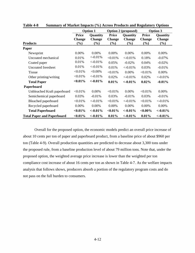
4-12

Table 4-8 Summary of Market Impacts (%) Across Products and Regulatory Options Option 1 Option 2 (proposed) Option 3

Products

Price Change

(%)

Quantity Change

(%)

Price Change

(%)

Quantity Change

(%)

Price Change

(%)

Quantity Change

(%) Paper Newsprint 0.00% 0.00% 0.00% 0.00% 0.00% 0.00% Uncoated mechanical 0.01% <-0.01% <0.01% <-0.01% 0.18% -0.07% Coated paper 0.01% <-0.01% 0.05% -0.02% 0.04% -0.02% Uncoated freesheet 0.01% <-0.01% 0.01% <-0.01% 0.03% -0.01% Tissue <0.01% <0.00% <0.01% 0.00% <0.01% 0.00% Other printing/writing <0.01% <-0.01% 0.02% <-0.01% 0.02% <-0.01% Total Paper <0.01% <-0.01% 0.01% <-0.01% 0.02% -0.01% Paperboard Unbleached Kraft paperboard <0.01% 0.00% <0.01% 0.00% <0.01% 0.00% Semichemical paperboard 0.03% -0.01% 0.03% -0.01% 0.03% -0.01% Bleached paperboard <0.01% <-0.01% <0.01% <-0.01% <0.01% <-0.01% Recycled paperboard 0.00% 0.00% 0.00% 0.00% 0.00% 0.00% Total Paperboard <0.01% <-0.01% <0.01% <-0.01% <0.00% <-0.01% Total Paper and Paperboard <0.01% <-0.01% 0.01% <-0.01% 0.01% <-0.01% Overall for the proposed option, the economic models predict an overall price increase of

about 10 cents per ton of paper and paperboard product, from a baseline price of about $960 per

ton (Table 4-9). Overall production quantities are predicted to decrease about 3,300 tons under

the proposed rule, from a baseline production level of about 79 million tons. Note that, under the

proposed option, the weighted average price increase is lower than the weighted per ton

compliance cost increase of about 16 cents per ton as shown in Table 4-7. As the welfare impacts

analysis that follows shows, producers absorb a portion of the regulatory program costs and do

not pass on the full burden to consumers.

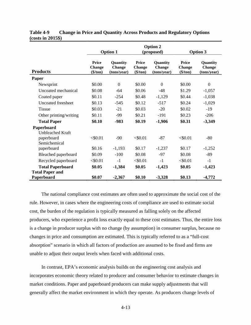
4-13

Table 4-9 Change in Price and Quantity Across Products and Regulatory Options (costs in 2015$)

Option 1 Option 2

(proposed) Option 3

Products

Price Change ($/ton)

Quantity Change

(tons/year)

Price Change ($/ton)

Quantity Change

(tons/year)

Price Change ($/ton)

Quantity Change

(tons/year) Paper Newsprint $0.00 0 $0.00 0 $0.00 0 Uncoated mechanical $0.08 -64 $0.06 -48 $1.29 -1,057 Coated paper $0.11 -254 $0.48 -1,129 $0.44 -1,038 Uncoated freesheet $0.13 -545 $0.12 -517 $0.24 -1,029 Tissue $0.03 -21 $0.03 -20 $0.02 -19 Other printing/writing $0.11 -99 $0.21 -191 $0.23 -206 Total Paper $0.10 -983 $0.19 -1,906 $0.31 -3,349 Paperboard

Unbleached Kraft paperboard <$0.01 -90 <$0.01 -87 <$0.01 -80

Semichemical paperboard $0.16 -1,193 $0.17 -1,237 $0.17 -1,252

Bleached paperboard $0.09 -100 $0.08 -97 $0.08 -89 Recycled paperboard <$0.01 -1 <$0.01 -1 <$0.01 -1 Total Paperboard $0.05 -1,384 $0.05 -1,423 $0.05 -1,423 Total Paper and Paperboard $0.07 -2,367 $0.10 -3,328 $0.13 -4,772

The national compliance cost estimates are often used to approximate the social cost of the

rule. However, in cases where the engineering costs of compliance are used to estimate social

cost, the burden of the regulation is typically measured as falling solely on the affected

producers, who experience a profit loss exactly equal to these cost estimates. Thus, the entire loss

is a change in producer surplus with no change (by assumption) in consumer surplus, because no

changes in price and consumption are estimated. This is typically referred to as a “full-cost

absorption” scenario in which all factors of production are assumed to be fixed and firms are

unable to adjust their output levels when faced with additional costs.

In contrast, EPA’s economic analysis builds on the engineering cost analysis and

incorporates economic theory related to producer and consumer behavior to estimate changes in

market conditions. Paper and paperboard producers can make supply adjustments that will

generally affect the market environment in which they operate. As producers change levels of

4-14

product supply in response to a regulation, consumers are typically faced with changes in prices

that cause them to alter the quantity they are willing to purchase. These changes in price and

output from the market model are used to estimate the total economic surplus changes for two

types of stakeholders: paper and paperboard consumers and producers.

As shown in Table 4-10, under the proposed Option 2, paper and paperboard consumers

are predicted to experience a $7.4 million reduction in surplus as the result of higher prices and

reduced consumption. Producer surplus is predicted to decrease about $5.6 million. Total welfare

losses are then estimated at $13 million.

Table 4-10 Summary of Consumer and Producer Surplus Changes in 2015 (millions 2015$) Surplus Change (in 2015 dollars) Option Product Type Consumer Producer Total

Option 1 Paper -$2.5 -$2.0 -$4.5 Paperboard -$2.2 -$3.0 -$5.3 Total -$4.8 -$5.0 -$9.8

Option 2 (proposed) Paper -$5.1 -$2.5 -$7.6 Paperboard -$2.3 -$3.1 -$5.4 Total -$7.4 -$5.6 -$13

Option 3 Paper -$7.8 -$6.2 -$13.9 Paperboard -$2.3 -$3.1 -$5.4 Total -$10 -$9.3 -$19.3

4.2.6 Limitations

Ultimately, the regulatory program may cause negligible increases in the costs of

supplying paper and paperboard products to consumers. The partial equilibrium model used in

this EIA is designed to evaluate behavioral responses to this change in costs within an

equilibrium setting within nationally competitive markets. The partial equilibrium model does

not model international trade. The national competitive market assumption is clearly very strong

because the markets in paper products may be regional for some products, as well as some

product markets within the paper industry may be interdependent. Regional price and quantity

impacts could be different from the average impacts reported if local market structures,

4-15

production costs, or demand conditions are substantially different from those used in this

analysis.

4.3 Small Business Impacts Analysis

The Regulatory Flexibility Act as amended by the Small Business Regulatory Enforcement

Fairness Act (SBREFA) generally requires an agency to prepare a regulatory flexibility analysis

of any rule subject to notice and comment rulemaking requirements under the Administrative

Procedure Act or any other statute, unless the agency certifies that the rule will not have a

significant economic impact on a substantial number of small entities. Small entities include

small businesses, small governmental jurisdictions, and small not-for-profit enterprises.

After considering the economic impact of the proposed regulatory options on small

entities, the screening analysis indicates that these proposed amendments will not have a

significant economic impact on a substantial number of small entities (SISNOSE). The

supporting analyses for these determinations are presented in this section of the EIA.

4.3.1 Small Business National Overview

The industry sectors covered by the proposed amendments were identified during the

development of the engineering cost analysis. The U.S. Census Bureau’s Statistics of U.S.

Businesses (SUSB) provides national information on the distribution of economic variables by

industry and enterprise size. The Census Bureau and the Office of Advocacy of the Small

Business Administration (SBA) supported and developed these files for use in a broad range of

economic analyses.6 Statistics include the total number of establishments, and receipts for all

entities in an industry; however, many of these entities may not necessarily be covered by the

proposed amendments. SUSB also provides statistics by enterprise employment and receipt size.

The Census Bureau’s definitions used in the SUSB are as follows:

Establishment: A single physical location where business is conducted or where services or industrial operations are performed.

Firm: A firm is a business organization consisting of one or more domestic establishments in the same state and industry that were specified under common

6See http://www.census.gov/csd/susb/ and http://www.sba.gov/advocacy/ for additional details.

4-16

ownership or control. The firm and the establishment are the same for single-establishment firms. For each multi-establishment firm, establishments in the same industry within a state will be counted as one firm- the firm employment and annual payroll are summed from the associated establishments.

Receipts: Receipts (net of taxes) are defined as the revenue for goods produced, distributed, or services provided, including revenue earned from premiums, commissions and fees, rents, interest, dividends, and royalties. Receipts exclude all revenue collected for local, state, and federal taxes.

Enterprise: An enterprise is a business organization consisting of one or more domestic establishments that were specified under common ownership or control. The enterprise and the establishment are the same for single-establishment firms. Each multi-establishment company forms one enterprise—the enterprise employment and annual payroll are summed from the associated establishments. Enterprise size designations are determined by the sum of employment of all associated establishments.

Because the SBA’s business size definitions apply to an establishment’s “ultimate parent

company,” we assumed in this analysis that the “firm” definition above is consistent with the

concept of ultimate parent company that is typically used for SBREFA screening analyses, and

the terms are used interchangeably.

4-17

4.3.2 Small Entity Economic Impact Measures

The proposed amendments will affect the owners of the facilities that will incur

compliance costs. The owners, either firms or individuals, are the entities that will bear the

financial impacts associated with these additional operating costs. The proposed amendments

have the potential to impact all firms owning affected facilities, both large and small.

The analysis provides EPA with an estimate of the magnitude of impacts the proposed

amendments may have on the ultimate parent companies that own facilities EPA expects might

be impacted by the proposed amendments. The analysis focuses on small firms because they may

have more difficulty complying with a proposed regulation or affording the costs associated with

meeting a revised standard. This section presents the data sources used in the screening analysis,

the methodology we applied to develop estimates of impacts, the results of the analysis, and

conclusions drawn from the results.

The small business impacts analysis relies upon a series of firm-level sales tests

(represented as cost-to-sales ratios) for firms that are likely to be associated with NAICS codes

322110 (pulp mills), 322121 (paper mills), and 322130 (paperboard mills). EPA obtained firm-

level employment, revenues, and production levels using various sources, including Hoovers, a

Dun & Bradstreet database, Manta, and corporate websites. Using these data, we estimated firm-

level compliance cost impacts and calculated cost-to-sales ratios to identify small firms that

might be significantly impacted by the proposed amendments.

For the sales test, we divided the estimates of annualized establishment compliance costs

at the company-level by estimates of ultimate parent company sales. This is known as the cost-

to-revenue ratio, or the “sales test.” The “sales test” is the impact methodology EPA employs in

analyzing small entity impacts as opposed to a “profits test,” in which annualized compliance

costs are calculated as a share of profits. The sales test is often used because revenues or sales

data are commonly available for entities impacted by EPA regulations, and profits data normally

made available are often not the true profit earned by firms because of accounting and tax

considerations. Revenues and sales as typically published are correct figures and are more

reliably reported when compared to profit data. The use of a “sales test” for estimating small

4-18

business impacts for a rulemaking such as this one is consistent with guidance offered by EPA

on compliance with SBREFA7 and is consistent with guidance published by the U.S. SBA’s

Office of Advocacy that suggests that cost as a percentage of total revenues is a metric for

evaluating cost increases on small entities in relation to increases on large entities.8

4.3.3 Small Entity Economic Impact Analysis and Conclusions

As discussed in Section 3, 108 facilities are potentially affected by each of the regulatory

options, but as the options increase in stringency the relative impacts increase. Of these 108

facilities, three are owned by small entities. Table 4-11 presents facility names, ultimate owners,

number of employees, and estimated sales in 2015 for the three small firms.

7 The SBREFA compliance guidance to EPA rulewriters regarding the types of small business analysis that should

be considered can be found at https://www.epa.gov/reg-flex/epas-action-development-process-final-guidance-epa-rulewriters-regulatory-flexibility-act. See Table 2 on page 24 of EPA’s Action Development Process, Final Guidelines for EPA Rulewriters: Regulatory Flexibility Act for guidance on interpretations of the magnitude of the cost-to-sales numbers.

8 U.S. SBA, Office of Advocacy. A Guide for Government Agencies, How to Comply with the Regulatory Flexibility Act, Implementing the President’s Small Business Agenda and Executive Order 13272, May 2012 (https://www.sba.gov/sites/default/files/rfaguide_0512_0.pdf).

4-19

Table 4-11 Potentially Affected Small Entities: Employees and Sales, 2015

Facility Ultimate Owner Employees in

2015 Sales in 2015

(million of 2015$) Cascade Pacific Pulp, LLC Cascade Pacific Pulp, LLC 185 66 Finch Paper LLC Finch Paper Holdings LLC 7509 89 Woodland Pulp LLC Woodland Pulp LLC 300 132

Table 4-12 shows that cost-to-sales ratios do not exceed 1 percent for any of the affected

small firms for the proposed option.

Table 4-12 Estimated Annualized Engineering Costs for Potentially Affected Small Entities across Regulatory Options (costs in 2015$)

Option 1

(less stringent) Option 2 (proposed) Option 3

(more stringent)

Ultimate Owner

Estimated Annualized

Costs ($)

Estimated Costs to

Sales Ratio

Estimated Annualized

Costs ($)

Estimated Costs to

Sales Ratio

Estimated Annualized

Costs ($)

Estimated Costs to

Sales Ratio Cascade Pacific Pulp, LLC 30,020 0.05% 161,094 0.2% 161,094 0.2% Finch Paper Holdings LLC 14,460 0.02% 14,460 0.02% 14,460 0.02% Woodland Pulp LLC 30,020 0.02% 30,020 0.02% 1,173,770 0.9%

EPA concludes from this analysis that a substantial number of small firms are not

significantly impacted. Based upon the analysis in this section, we conclude there is no

SISNOSE arising from the proposed amendments.

9 The small business size threshold for NAICS 322121 (paper mills) is 1,250 employees.

4-20

4.4 Employment Impacts Analysis

While a standalone analysis of employment impacts is not included in a standard cost-

benefit analysis, such an analysis is of particular concern in the current economic climate given

continued interest in the employment impact of regulations such as this proposed rule. Executive

Order 13563, states, “Our regulatory system must protect public health, welfare, safety, and our

environment while promoting economic growth, innovation, competitiveness, and job

creation.”10 A discussion of compliance costs, including reporting and recordkeeping

requirements, is included in Section 3 of this EIA. This section presents an overview of the

various ways that environmental regulation can affect employment. EPA continues to explore the

relevant theoretical and empirical literature and to seek public comments in order to ensure that

the way EPA characterizes the employment effects of its regulations is valid and informative.11

4.4.1 Employment Impacts of Environmental Regulation

From an economic perspective, labor is an input into producing goods and services; if a

regulation requires that more labor be used to produce a given amount of output, that additional

labor is reflected in an increase in the cost of production. Moreover, when the economy is at full

employment, we would not expect an environmental regulation to have a net impact on overall

employment because labor is being shifted from one sector to another. On the other hand, in

periods of high unemployment, net employment effects (both positive and negative) are possible.

For example, an increase in labor demand due to regulation may result in a short-term net

increase in overall employment as workers are hired by the regulated sector to help meet new

requirements (e.g., to install new equipment) or by the environmental protection sector to

produce new abatement capital resulting in hiring previously unemployed workers. When

significant numbers of workers are unemployed, the opportunity costs associated with displacing

jobs in other sectors are likely to be higher. And, in general, if a regulation imposes high costs

10 Executive Order 13563 (January 21, 2011). Improving Regulation and Regulatory Review. Section 1. General

Principles of Regulation, Federal Register, Vol. 76, Nr. 14, p. 3821. 11 The employment analysis in this RIA is part of EPA’s ongoing effort to “conduct continuing evaluations of potential loss or shifts of employment which may result from the administration or enforcement of [the Act]” pursuant to CAA section 321(a).

4-21

and does not increase the demand for labor, it may lead to a decrease in employment. The

responsiveness of industry labor demand depends on how these forces all interact. Economic

theory indicates that the responsiveness of industry labor demand depends on a number of

factors: price elasticity of demand for the product, substitutability of other factors of production,

elasticity of supply of other factors of production, and labor’s share of total production costs.

Berman and Bui (2001) put this theory in the context of environmental regulation, and suggest

that, for example, if all firms in the industry are faced with the same compliance costs of

regulation and product demand is inelastic, then industry output may not change much at all.

Regulations set in motion new orders for pollution control equipment and services. New

categories of employment have been created in the process of implementing environmental

regulations. When a regulation is promulgated, one typical response of industry is to order

pollution control equipment and services in order to comply with the regulation when it becomes

effective. On the other hand, the closure of plants that choose not to comply – and any changes in

production levels at plants choosing to comply and remain in operation - occur after the

compliance date, or earlier in anticipation of the compliance obligation. Environmental

regulation may increase revenue and employment in the environmental technology industry.

While these increases represent gains for that industry, they translate into costs to the regulated

industries required to install the equipment.

Environmental regulations support employment in many basic industries. Regulated firms

either hire workers to design and build pollution controls directly or purchase pollution control

devices from a third party for installation. Once the equipment is installed, regulated firms hire

workers to operate and maintain the pollution control equipment—much like they hire workers

to produce more output. In addition to the increase in employment in the environmental

protection industry (via increased orders for pollution control equipment), environmental

regulations also support employment in industries that provide intermediate goods to the

environmental protection industry. The equipment manufacturers, in turn, order steel, tanks,

vessels, blowers, pumps, and chemicals to manufacture and install the equipment.

Berman and Bui (2001) demonstrate using standard neoclassical microeconomics that

environmental regulations have an ambiguous effect on employment in the regulated sector. The

4-22

theoretical results imply that the effect of environmental regulation on employment in the

regulated sector is an empirical question. Berman and Bui (2001) developed an innovative

approach to examine how an increase in local air quality regulation that reduces nitrogen oxides

(NOX) emissions affects manufacturing employment in the South Coast Air Quality

Management District (SCAQMD), which incorporates Los Angeles and its suburbs. During the

time frame of their study, 1979 to 1992, the SCAQMD enacted some of the country’s most

stringent air quality regulations. Using SCAQMD’s local air quality regulations, Berman and Bui

identify the effect of environmental regulations on net employment in the regulated industries.12

The authors find that “while regulations do impose large costs, they have a limited effect on

employment” (Berman and Bui, 2001, p. 269). Their conclusion is that local air quality

regulation “probably increased labor demand slightly” but that “the employment effects of both

compliance and increased stringency are fairly precisely estimated zeros, even when exit and

dissuaded entry effects are included” (Berman and Bui, 2001, p. 269).13

While there is an extensive empirical, peer-reviewed literature analyzing the effect of

environmental regulations on various economic outcomes including productivity, investment,

competitiveness as well as environmental performance, there are only a few papers that examine

the impact of environmental regulation on employment, but this area of the literature has been

growing. As stated previously in this EIA section, empirical results from Berman and Bui (2001)

suggest that new or more stringent environmental regulations do not have a substantial impact on

net employment (either negative or positive) in the regulated sector. Similarly, Ferris,

Shadbegian, and Wolverton (2014) also find that regulation-induced net employment impacts are

close to zero in the regulated sector. Furthermore, Gray et al (2014) find that pulp mills that had

to comply with both the air and water regulations in EPA’s 1998 “Cluster Rule” experienced

relatively small and not always statistically significant, decreases in employment. Nevertheless,

other empirical research suggests that more highly regulated counties may generate fewer jobs

than less regulated ones (Greenstone 2002, Walker 2011). However, the methodology used in

these two studies cannot estimate whether aggregate employment is lower or higher due to more

stringent environmental regulation, it can only imply that relative employment growth in some

12 Berman and Bui include over 40 4-digit SIC industries in their sample. 13 Including the employment effect of exiting plants and plants dissuaded from opening will increase the estimated

impact of regulation on employment.

4-23

sectors differs between more and less regulated areas. List et al. (2003) find some evidence that

this type of geographic relocation, from more regulated areas to less regulated areas may be

occurring. Overall, the peer-reviewed literature does not contain evidence that environmental

regulation has a large impact on net employment (either negative or positive) in the long run

across the whole economy.

While the theoretical framework laid out by Berman and Bui (2001) still holds for the

industry affected under these proposed amendments, important differences in the markets and

regulatory settings analyzed in their study and the setting presented here lead us to conclude that

it is inappropriate to use their quantitative estimates to estimate the net employment impacts

from these proposed amendments. In particular, the industries used in these two studies as well

as the timeframe (late 1970’s to early 1990’s) are quite different than those in this proposal.

The preceding sections have outlined the challenges associated with estimating net

employment effects in the regulated sector and in the environmental protection sector. These

challenges make it very difficult to accurately produce net employment estimates for the whole

economy that would appropriately capture the way in which costs, compliance spending, and

environmental benefits propagate through the macro-economy. Given the difficulty with

estimating national impacts of regulations, EPA has not generally estimated economy-wide

employment impacts of its regulations in its benefit-cost analyses. However, in its continuing

effort to advance the evaluation of costs, benefits, and economic impacts associated with

environmental regulation, EPA has formed a panel of experts as part of EPA’s Science Advisory

Board (SAB) to advise EPA on the technical merits and challenges of using economy-wide

economic models to evaluate the impacts of its regulations, including the impact on net national

employment.14 Once EPA receives guidance from this panel it will carefully consider this input

and then decide if and how to proceed on economy-wide modeling of net employment impacts of

its regulations.

14 For further information see:

http://yosemite.epa.gov/sab/sabproduct.nsf/0/07E67CF77B54734285257BB0004F87ED?OpenDocument

4-24

4.4.2 Labor Estimates Associated with Proposed Amendments

The labor estimates associated with the options for opacity limit changes for recovery

furnaces and lime kilns, as well as the incremental increases in recordkeeping and reporting are

presented below in Table 4-13. We convert estimates of the number hours of labor required to

full-time equivalents (FTEs) by dividing by 2,080 (40 hours per week multiplied by 52 weeks).

We note that this type of FTE estimate cannot be used to make assumptions about the specific

number of people involved or whether new jobs are created for new employees. In this EIA, we

make no distinction in the quantitative estimates between labor changes within and outside of the

regulated sector.

Table 4-13 Labor-based Employment Estimates for Operating and Maintaining Control Equipment Requirements, across Proposed Regulatory Options

Option 1 (less) Option 2

(proposed) Option 3 (more)

Recovery Furnace Opacity Limit Proposed Amendments

Nationwide Labor (hrs) 2,100 4,200 6,800

Full-time Equivalents (FTE) 1 2 3 Incremental Reporting and Recordkeeping

Nationwide Labor (hrs) 12,464 12,464 12,464

Full-time Equivalents (FTE) 6 6 6 Total

Nationwide Labor (hrs) 14,564 16,664 19,264 Full-time Equivalents (FTE) 7 8 9

5-1

5 REFERENCES

BE&K Engineering. 2001. Emission Control Study – Technology Cost Estimates. Main document, appendices. Prepared for American Forest & Paper Association. September 2001.

Berck, P., Hoffmann, S., 2002. Assessing the Employment Impacts of Environmental and Natural Resource Policy. Environmental and Resource Economics 22(1): 133-156.

Bezdek, R.H., Wendling, R.M., DiPerna, P., 2008. Environmental protection, the economy, and jobs: National and regional analyses. Journal of Environmental Management 86(1): 63-79.

Berman, E. and L. T. M. Bui. 2001. “Environmental Regulation and Labor Demand: Evidence from the South Coast Air Basin.” Journal of Public Economics 79(2): 265-295, docket nr. EPA-HQ-OAR-2011-0135 at <http://www.regulations.gov>

Clearwater Paper. 2016. "2015 Annual Report." <http://files.shareholder.com/downloads/ABEA-

23EJ0Z/2716808938x0x882397/1E582464-FDB3-4F69-ABD2-80DFE68210B9/CLW_2015_Annual_Report_web_bmk.pdf>

Ferris, A., R.J. Shadbegian, and A. Wolverton. 2014. “The Effect of Environmental Regulation

on Power Sector Employment: Phase I of the Title IV SO2 Trading Program.” Journal of the Association of Environmental and Resource Economists 5:173-193.

Fullerton, D., Metcalf, G., 2002. Tax Incidence. In Handbook of Public Economics, eds A. Auerbach, M. Feldstein. Elsevier: Amsterdam.

Gray, W.B., R.J. Shadbegian, C. Wang, and M. Meral. 2014. “Do EPA Regulations Affect Labor Demand? Evidence from the Pulp and Paper Industry.” Journal of Environmental Economics and Management: 68, 188-202.

Greenstone, M. 2002. “The Impacts of Environmental Regulations on Industrial Activity:

Evidence from the 1970 and 1977 Clean Air Act Amendments and the Census of Manufactures.” Journal of Political Economy 110(6): 1175-1219.

Ince, P., Buongiorno, J., 2007. North American Pulp and Paper Model (NAPAP). In Resource

and Market Projections for Forest Policy Development: Twenty-five Years of Experience with the US RPA Timber Assessment, eds D.M. Adams, R.W. Haynes, pp. 99-174. Springer: Dordrecht, The Netherlands.

5-2

Hanks, K. and T. Holloway. Costs/Impacts of the Subpart MM Residual Risk and Technology Review. Memorandum to K. Spence, U.S. Environmental Protection Agency. August 19, 2016.

Holloway, T. and K. Hanks. Emissions Inventory for Kraft Pulp Mills and Costs/Impacts of the Section 111(b) Review of the Kraft Pulp Mills NSPS. Memorandum to K. Spence and B. Schrock, U.S. Environmental Protection Agency. February 4, 2013.

RISI Inc., March 20, 2015a. Price Watch. PPI Pulp & Paper Week 37(11): 3-5.

RISI Inc., June 19, 2015b. Price Watch. PPI Pulp & Paper Week 37(24): 3-5.

RISI Inc., September 25, 2015c. Price Watch. PPI Pulp & Paper Week 37(37): 3.

RISI Inc., December 18, 2015d. Price Watch. PPI Pulp & Paper Week 37(48): 3.

RISI Inc., February 12, 2016. Price Watch. PPI Pulp & Paper Week 38(6): 8.

List, J. A., D. L. Millimet, P. G. Fredriksson, and W. W. McHone. 2003. “Effects of Environmental Regulations on Manufacturing Plant Births: Evidence from a Propensity Score Matching Estimator.” The Review of Economics and Statistics 85(4): 944-952.

U.S. Energy Information Administration, 2016. Assumptions to the Annual Energy Outlook 2016: With Projections for 2040.<http://www.eia.gov/forecasts/aeo/pdf/0383(2016).pdf>.

U.S. Environmental Protection Agency, 2002. Profile of the Pulp and Paper Industry. Sector Notebook Project. EPA/310-R-02-002. <http://www.epa.gov/Compliance/resources/publications/assistance/sectors/notebooks/index.html>. Accessed on: 11/14/11.

U.S. Environmental Protection Agency. 2016. Technical Memorandum from K. Spence to Docket EPA-HQ-OAR-2014-0741. Review of the Continuous Opacity Monitoring System Data from the Pulp and Paper ICR Responses for Subpart MM Sources. Draft, June 14, 2016.

U.S. Environmental Protection Agency, 2010. Guidelines for Preparing Economic Analyses, EPA 240-R-10-001. <http://yosemite.epa.gov/ee/epa/eed.nsf/pages/Guidelines.html> Accessed on: 11/14/11.

U.S. Environmental Protection Agency, Office of Water, Office of Air and Radiation, 1993. Economic Impact and Regulatory Flexibility Analysis of Proposed Effluent Guidelines and NESHAP for the Pulp, Paper, and Paperboard Industry: Final Report, 821R93021.

5-3

Walker, R. 2011. “Environmental Regulation and Labor Reallocation." American Economic

Review: 101(3):442-447.