ECONOMIA DEGLI INTERMEDIARI FINANZIARI AVANZATA

1

MODULO ASSET MANAGEMENT

LECTURE 3

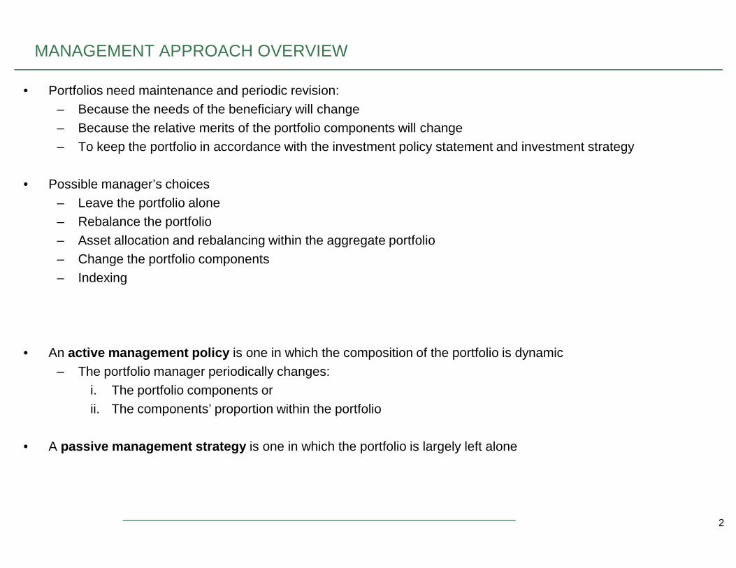
• Portfolios need maintenance and periodic revision:– Because the needs of the beneficiary will change– Because the relative merits of the portfolio components will change– To keep the portfolio in accordance with the investment policy statement and investment strategy

• Possible manager’s choices– Leave the portfolio alone– Rebalance the portfolio– Asset allocation and rebalancing within the aggregate portfolio– Change the portfolio components– Indexing

MANAGEMENT APPROACH OVERVIEW

2

– Indexing

• An active management policy is one in which the composition of the portfolio is dynamic– The portfolio manager periodically changes:

i. The portfolio components orii. The components’ proportion within the portfolio

• A passive management strategy is one in which the portfolio is largely left alone

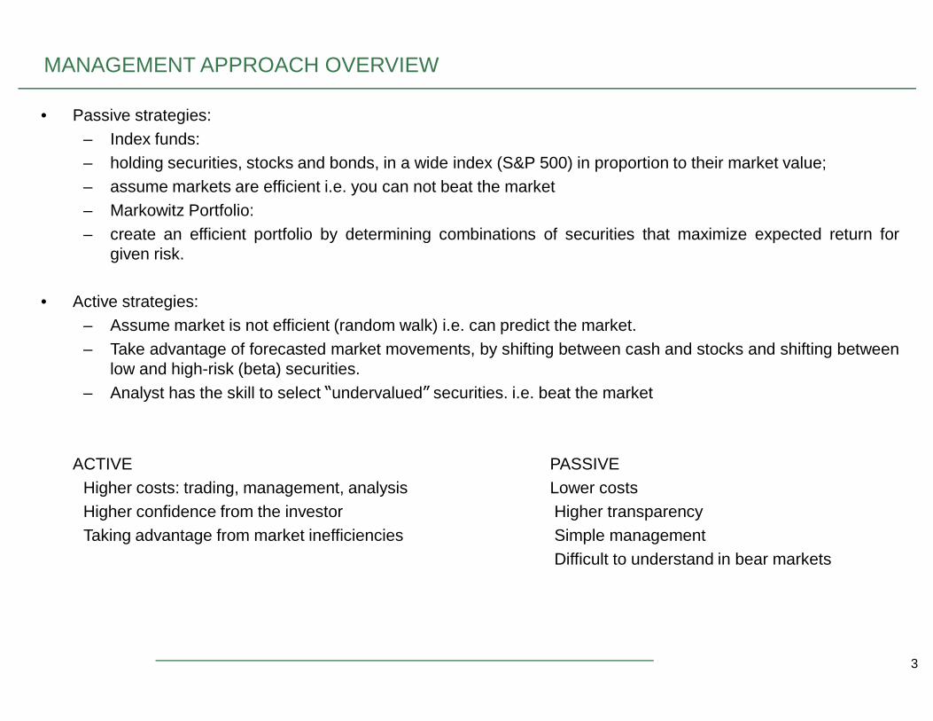
• Passive strategies:– Index funds:– holding securities, stocks and bonds, in a wide index (S&P 500) in proportion to their market value;– assume markets are efficient i.e. you can not beat the market– Markowitz Portfolio:– create an efficient portfolio by determining combinations of securities that maximize expected return for

given risk.

• Active strategies:– Assume market is not efficient (random walk) i.e. can predict the market.– Take advantage of forecasted market movements, by shifting between cash and stocks and shifting between

low and high-risk (beta) securities.

MANAGEMENT APPROACH OVERVIEW

3

low and high-risk (beta) securities.– Analyst has the skill to select “undervalued” securities. i.e. beat the market

ACTIVE PASSIVEHigher costs: trading, management, analysis Lower costsHigher confidence from the investor Higher transparencyTaking advantage from market inefficiencies Simple management

Difficult to understand in bear markets

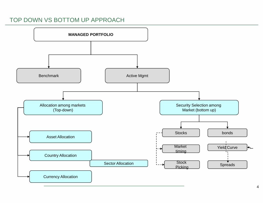
Benchmark Active Mgmt

MANAGED PORTFOLIO

TOP DOWN VS BOTTOM UP APPROACH

4

Sector Allocation

Security Selection among Market (bottom up)

Stocks bonds

Market timing

Yield Curve

Stock Picking

Spreads

Asset Allocation

Country Allocation

Currency Allocation

Allocation among markets (Top-down)

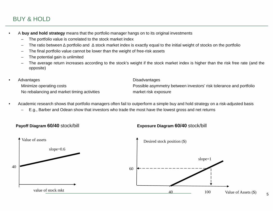
• A buy and hold strategy means that the portfolio manager hangs on to its original investments– The portfolio value is correlated to the stock market index– The ratio between ∆ portfolio and ∆ stock market index is exactly equal to the initial weight of stocks on the portfolio– The final portfolio value cannot be lower than the weight of free-risk assets– The potential gain is unlimited– The average return increases according to the stock’s weight if the stock market index is higher than the risk free rate (and the

opposite)

• Advantages DisadvantagesMinimize operating costs Possible asymmetry between investors’ risk tolerance and portfolioNo rebalancing and market timing activities market risk exposure

• Academic research shows that portfolio managers often fail to outperform a simple buy and hold strategy on a risk-adjusted basis

BUY & HOLD

5

• Academic research shows that portfolio managers often fail to outperform a simple buy and hold strategy on a risk-adjusted basis– E.g., Barber and Odean show that investors who trade the most have the lowest gross and net returns

Payoff Diagram 60/40 stock/bill

slope=0.6

value of stock mkt

Value of assets

40

Desired stock position ($)

Value of Assets ($)40

slope=1

100

60

Exposure Diagram 60/40 stock/bill

Rebalancing a portfolio is the process of periodically adjusting it to maintain the original conditionsRebalancing within the Portfolio• Constant mix strategy• Constant proportion portfolio insurance• Relative performance of constant mix and CPPI strategies

PORTFOLIO REBALANCING

6

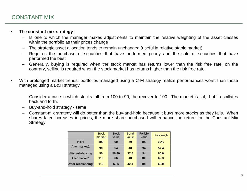
• The constant mix strategy:– Is one to which the manager makes adjustments to maintain the relative weighting of the asset classes

within the portfolio as their prices change– The strategic asset allocation tends to remain unchanged (useful in relative stable market)– Requires the purchase of securities that have performed poorly and the sale of securities that have

performed the best– Generally, buying is required when the stock market has returns lower than the risk free rate; on the

contrary, selling is required when the stock market has returns higher than the risk free rate.

• With prolonged market trends, portfolios managed using a C-M strategy realize performances worst than thosemanaged using a B&H strategy

– Consider a case in which stocks fall from 100 to 90, the recover to 100. The market is flat, but it oscillates

CONSTANT MIX

7

– Consider a case in which stocks fall from 100 to 90, the recover to 100. The market is flat, but it oscillatesback and forth.

– Buy-and-hold strategy - same– Constant-mix strategy will do better than the buy-and-hold because it buys more stocks as they falls. When

shares later increases in prices, the more share purchased will enhance the return for the Constant-MixStrategy

Stock market

Stock value

Bond value

Portfolio Value

Stock weight

Initial 100 60 40 100 60%

After market∆

90 54 40 94 57.4

After rebalancing 90 56.40 37.6 94 60.0

After market∆ 110 66 40 106 62.3

After rebalancing 110 63.6 42.4 106 60.0

100100

Por

tfolio

Val

ueP

ortfo

lio V

alue

Constant MixConstant Mix

BuyBuy--andand--HoldHold

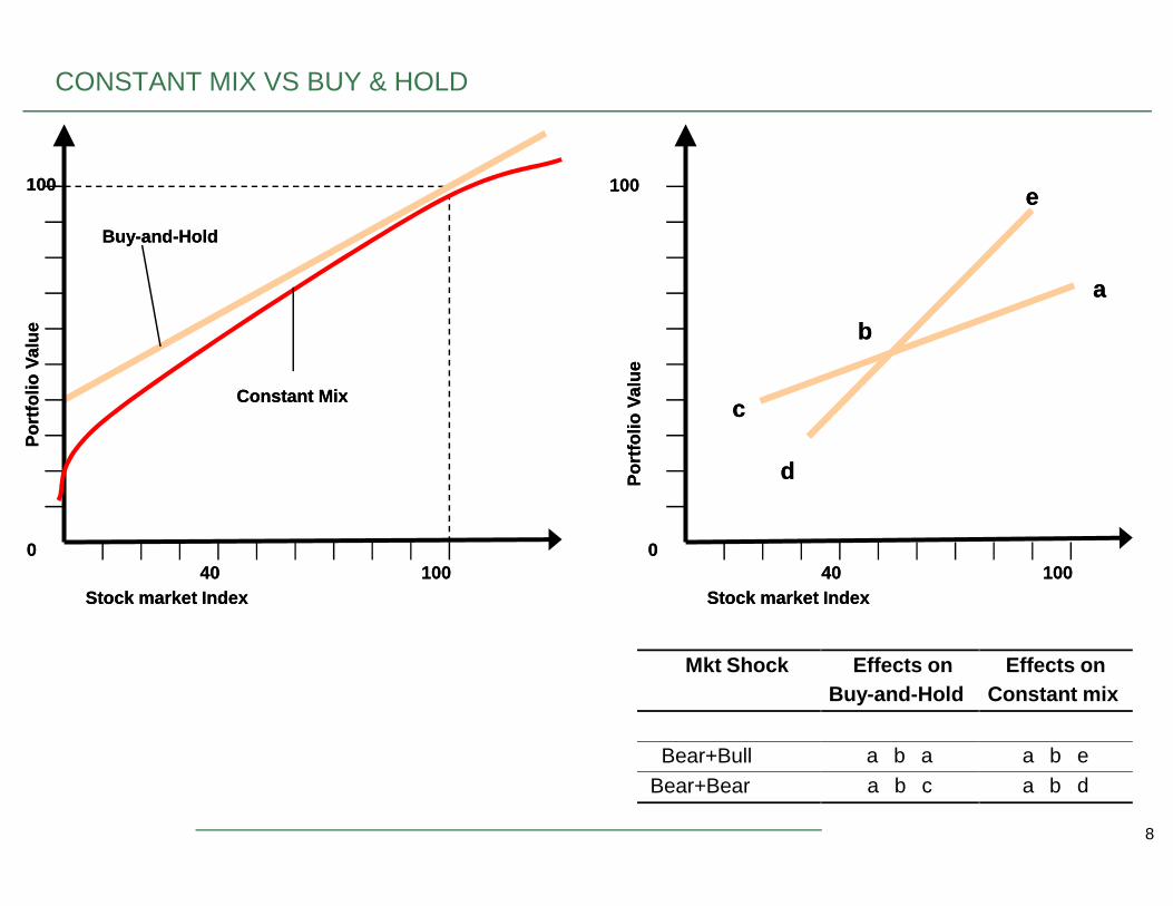
CONSTANT MIX VS BUY & HOLD

100100

Por

tfolio

Val

ueP

ortfo

lio V

alue

ee

bb

aa

cc

8

4040 10010000

Stock market IndexStock market Index4040 100100

00

Stock market IndexStock market Index

Por

tfolio

Val

ueP

ortfo

lio V

alue

dd

Mkt Shock Effects onBuy-and-Hold

Effects onConstant mix

Bear+Bull a b a a b e

Bear+Bear a b c a b d

DYNAMIC STRATEGIES

• Linear strategies (do nothing) determine linear payoff

• Dynamic strategies (do something) following the rule “buys stocks as they fall and sell stock as they rise” determineconcave payoff:

– Low elasticity in bullish markets– No protection floor– Useful in volatile markets

• Dynamic strategies (do something) following the rule “sell stocks as they fall …...” determine convex payoff:– High elasticity in bullish markets– Good protection

9

• Convex strategies represent the Purchase of portfolio insurance because it has a floor value;

• Concave strategies represent the sale of portfolio insurance

• Convex and concave strategies are mirror images of each other

TECNICHE DI PORTFOLIO INSURANCE

• Le tecniche gestionali rivolte all’ottenimento della protezione del capitale investito sono normalmente definitetecniche di Porfolio Insurance (PI).

• Gli elementi principali che le caratterizzano sono:– Portafoglio di riferimento (indici di borsa, titoli azionari, fondi comuni ...)– Livello di copertura (superiore, pari o inferiore al capitale versato)– Orizzonte temporale della copertura (3 anni – 10/15 anni)

• Le principali tecniche di portfolio insurance sono:– Buy and Hold (B&H)

10

– Buy and Hold (B&H)– Stop Loss (SLO)– Protective Call Strategy (PCS)– Protective Put Strategy (PPS)

– Constant Proportion (CPPI)

TECNICHE DI PORTFOLIO INSURANCE

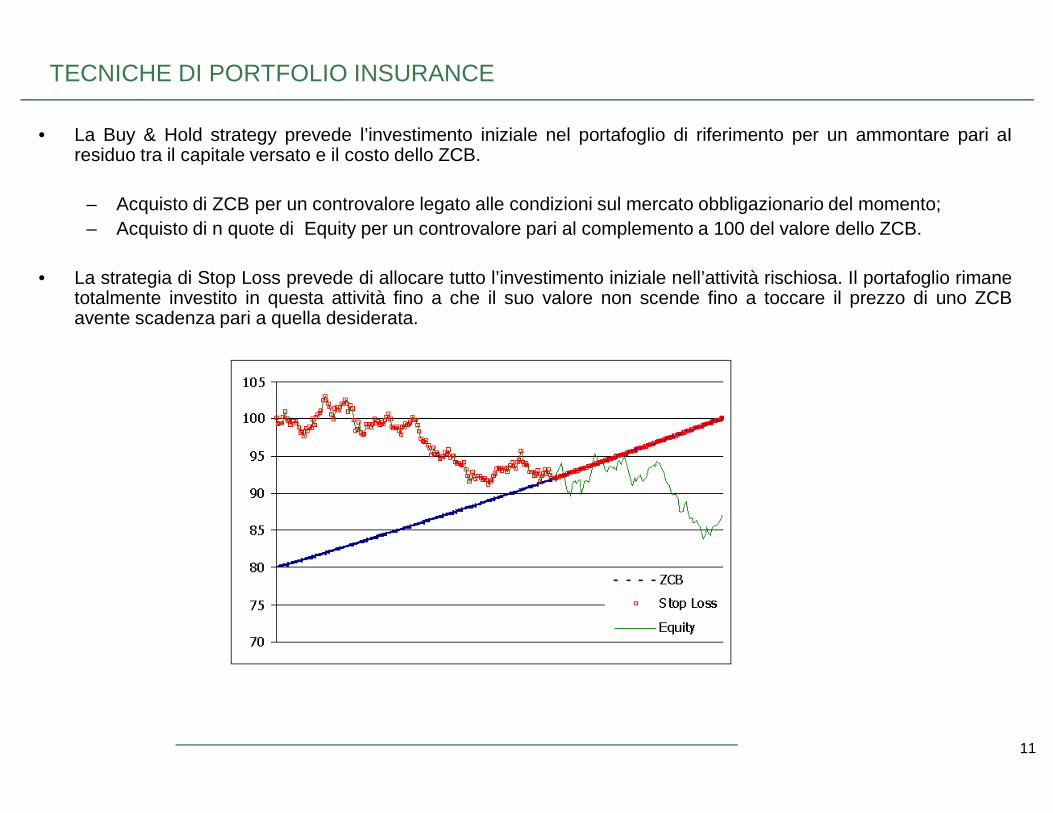
• La Buy & Hold strategy prevede l’investimento iniziale nel portafoglio di riferimento per un ammontare pari aIresiduo tra il capitale versato e il costo dello ZCB.

– Acquisto di ZCB per un controvalore legato alle condizioni sul mercato obbligazionario del momento;– Acquisto di n quote di Equity per un controvalore pari al complemento a 100 del valore dello ZCB.

• La strategia di Stop Loss prevede di allocare tutto l’investimento iniziale nell’attività rischiosa. Il portafoglio rimanetotalmente investito in questa attività fino a che il suo valore non scende fino a toccare il prezzo di uno ZCBavente scadenza pari a quella desiderata.

11

TECNICHE DI PORTFOLIO INSURANCE

• La Protective Put Strategy prevede l’investimento nella parte azionaria accompagnato all’acquisto di una opzioneput. La strutturazione del portafoglio comporta la determininazione del livello di strike price della PUT compatiblecon la protezione del capitale investito e la successiva determinazione della quantità di opzioni da acquistare

• La Protective Call Strategy prevede l’investimento in parte nello ZCB e per il rimanente in una opzione call.Rappresenta la struttura più diffusa sul mercato per ottenere protezione dell’investito:

• Le opzioni utilizzate in queste strutture si differenziano– per il metodo di misurazione della performance:

i. alla fine del periodo (tradizionale)ii. come media di periodo (asiatica)

– Per il sottostante oggetto di investimento:

12

– Per il sottostante oggetto di investimento:i. singolo assetii. basket di asset

– Per la presenza di meccanismi opzionali di path-dependencyi. rendimento basato su classifica performance (best/worst inside basket, rainbow)ii. barriera di attivazione/disattivazione dell’opzione (knock in/out)iii. consolidamento dei risultati (cliquet)

TECNICHE DI PORTFOLIO INSURANCE

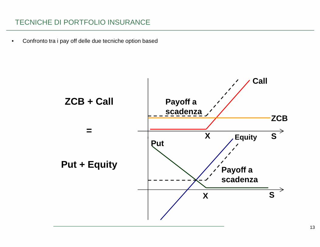
• Confronto tra i pay off delle due tecniche option based

Call

ZCB

Payoff a scadenza

ZCB + Call

13

X

X

PutEquity

Payoff a scadenza

Put + Equity

=S

S

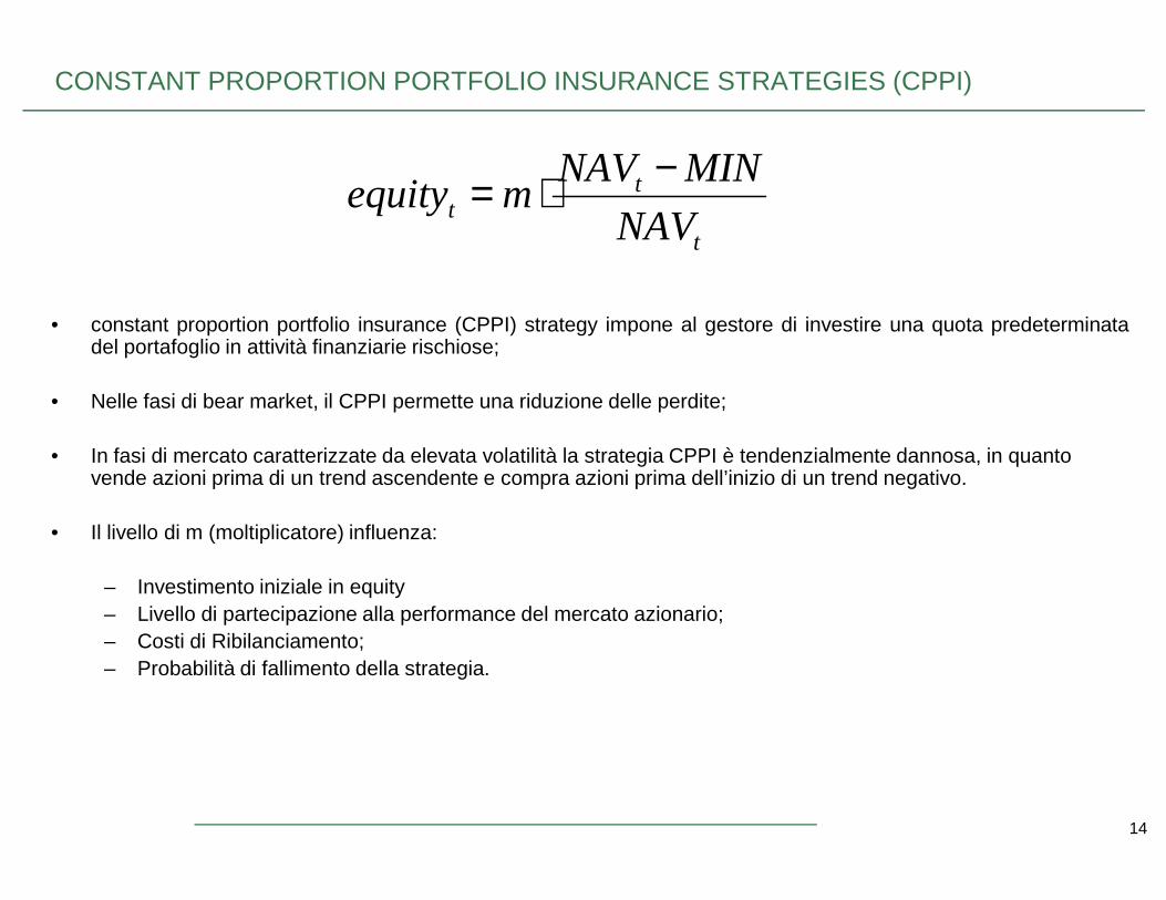
CONSTANT PROPORTION PORTFOLIO INSURANCE STRATEGIES (CPPI)

• constant proportion portfolio insurance (CPPI) strategy impone al gestore di investire una quota predeterminatadel portafoglio in attività finanziarie rischiose;

• Nelle fasi di bear market, il CPPI permette una riduzione delle perdite;

• In fasi di mercato caratterizzate da elevata volatilità la strategia CPPI è tendenzialmente dannosa, in quanto

t

tt NAV

MINNAVmequity

−⋅=

14

• In fasi di mercato caratterizzate da elevata volatilità la strategia CPPI è tendenzialmente dannosa, in quanto vende azioni prima di un trend ascendente e compra azioni prima dell’inizio di un trend negativo.

• Il livello di m (moltiplicatore) influenza:

– Investimento iniziale in equity– Livello di partecipazione alla performance del mercato azionario;– Costi di Ribilanciamento;– Probabilità di fallimento della strategia.

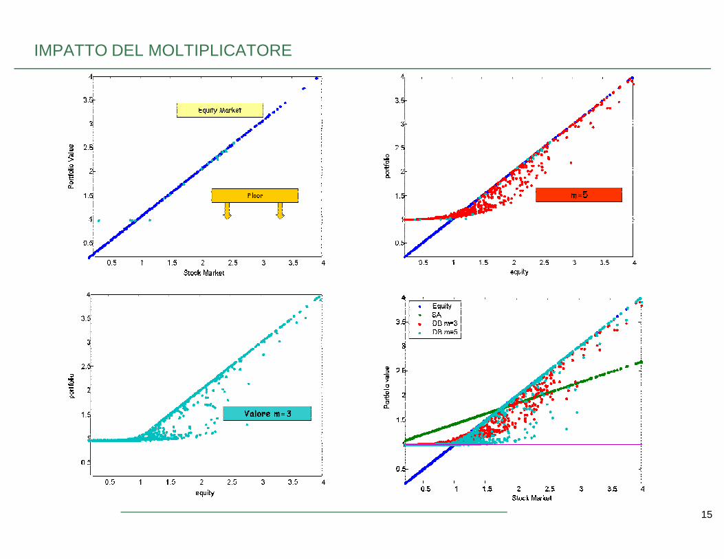
IMPATTO DEL MOLTIPLICATORE

15

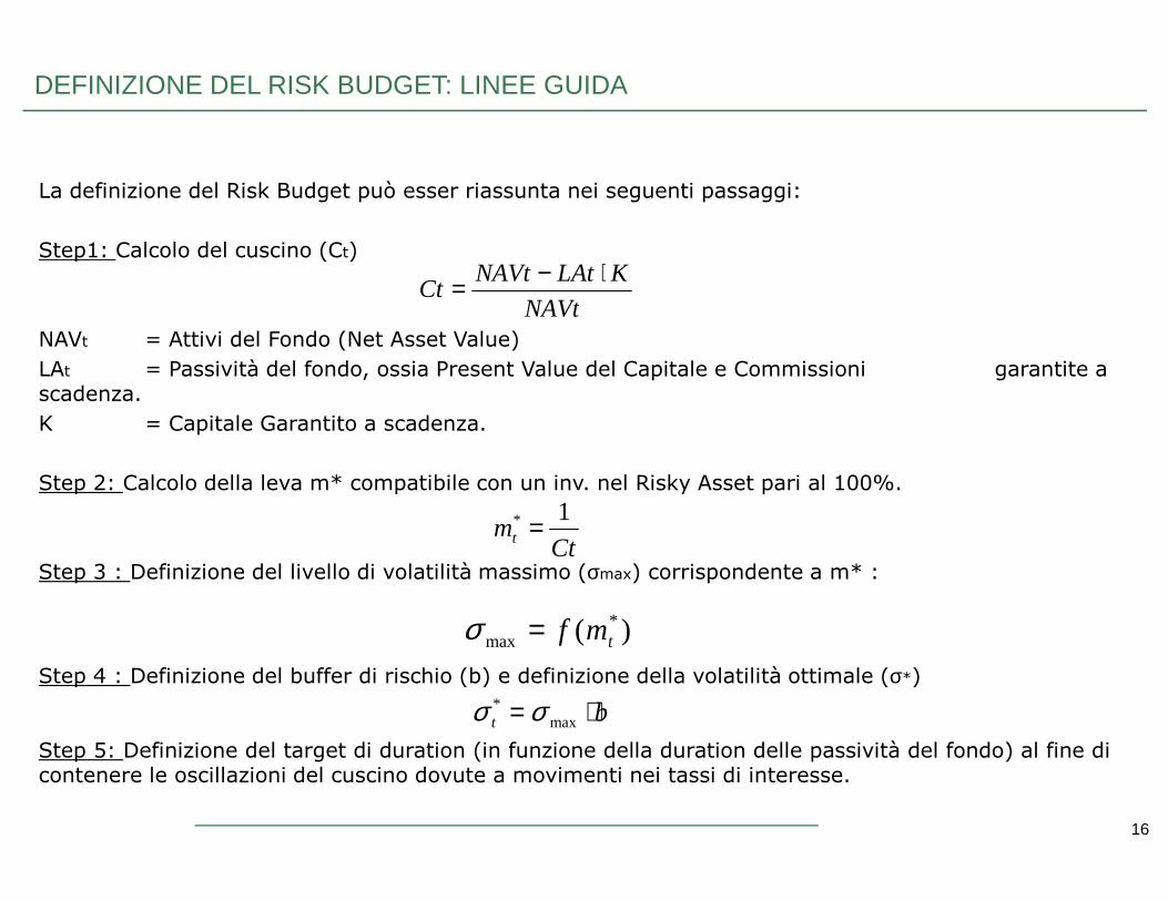
La definizione del Risk Budget può esser riassunta nei seguenti passaggi:

Step1: Calcolo del cuscino (Ct)

NAVt = Attivi del Fondo (Net Asset Value)

LAt = Passività del fondo, ossia Present Value del Capitale e Commissioni garantite a scadenza.

K = Capitale Garantito a scadenza.

DEFINIZIONE DEL RISK BUDGET: LINEE GUIDA

NAVt

KLAtNAVtCt

⋅−=

16

Step 2: Calcolo della leva m* compatibile con un inv. nel Risky Asset pari al 100%.

Step 3 : Definizione del livello di volatilità massimo (σmax) corrispondente a m* :

Step 4 : Definizione del buffer di rischio (b) e definizione della volatilità ottimale (σ*)

Step 5: Definizione del target di duration (in funzione della duration delle passività del fondo) al fine dicontenere le oscillazioni del cuscino dovute a movimenti nei tassi di interesse.

Ctmt

1* =

)( *max tmf=σ

bt ⋅= max* σσ

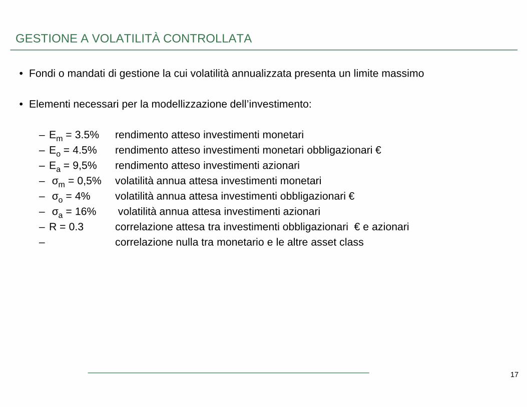
• Fondi o mandati di gestione la cui volatilità annualizzata presenta un limite massimo

• Elementi necessari per la modellizzazione dell’investimento:

– Em = 3.5% rendimento atteso investimenti monetari– Eo = 4.5% rendimento atteso investimenti monetari obbligazionari €– Ea = 9,5% rendimento atteso investimenti azionari– σm = 0,5% volatilità annua attesa investimenti monetari– σo = 4% volatilità annua attesa investimenti obbligazionari €

GESTIONE A VOLATILITÀ CONTROLLATA

17

o

– σa = 16% volatilità annua attesa investimenti azionari– R = 0.3 correlazione attesa tra investimenti obbligazionari € e azionari– correlazione nulla tra monetario e le altre asset class

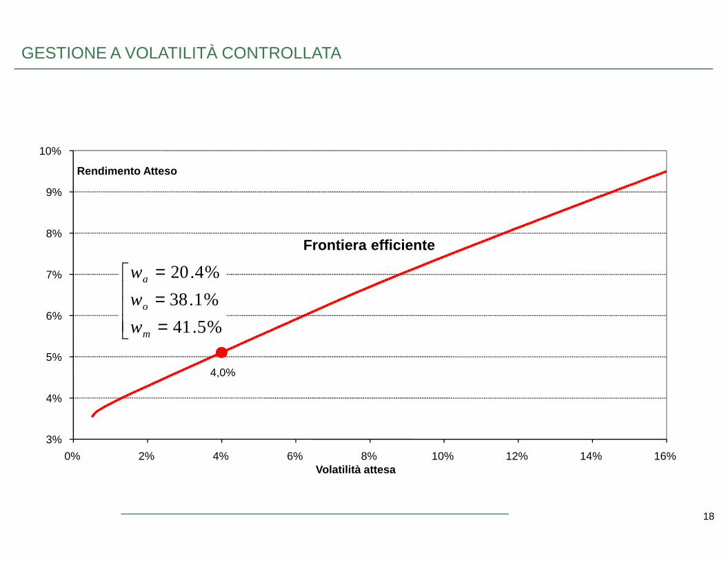
7%

8%

9%

10%

Rendimento Atteso

= %4.20aw

Frontiera efficiente

GESTIONE A VOLATILITÀ CONTROLLATA

18

4,0%

3%

4%

5%

6%

0% 2% 4% 6% 8% 10% 12% 14% 16%Volatilità attesa

===

%5.41

%1.38

%4.20

m

o

a

w

w

w

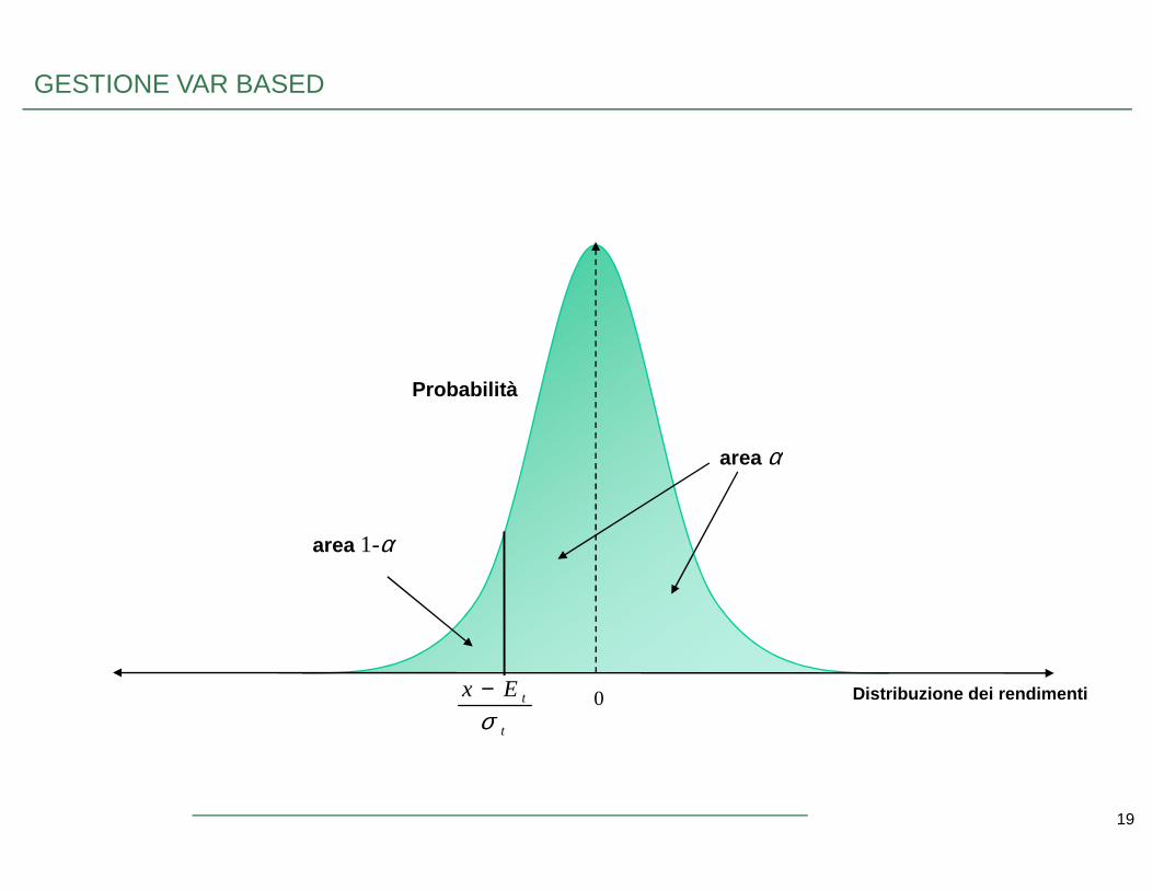
Probabilità

α

GESTIONE VAR BASED

19

t

tEx

σ− Distribuzione dei rendimenti 0

area 1-α

area α

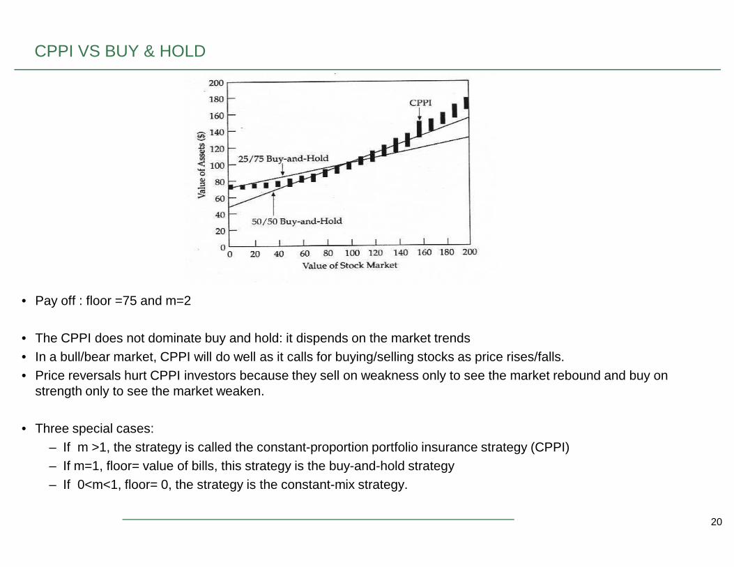
CPPI VS BUY & HOLD

20

• Pay off : floor =75 and m=2

• The CPPI does not dominate buy and hold: it dispends on the market trends• In a bull/bear market, CPPI will do well as it calls for buying/selling stocks as price rises/falls.• Price reversals hurt CPPI investors because they sell on weakness only to see the market rebound and buy on

strength only to see the market weaken.

• Three special cases:– If m >1, the strategy is called the constant-proportion portfolio insurance strategy (CPPI)– If m=1, floor= value of bills, this strategy is the buy-and-hold strategy– If 0<m<1, floor= 0, the strategy is the constant-mix strategy.

AT THE END ….

• In a rising market, the CPPI strategy outperforms CM

• In a declining market, the CPPI strategy outperforms CM

• In a flat market, neither strategy has an obvious advantage

• In a volatile market, the CM strategy outperforms CPPI

• The relative performance of the strategies depends on the performance of the market during the evaluation period

• In the long run, the market will probably rise, which favors CPPI; in the short run, the market will be volatile, which

21

• In the long run, the market will probably rise, which favors CPPI; in the short run, the market will be volatile, whichfavors CM

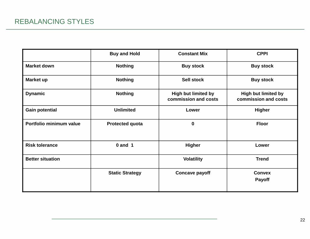
Buy and Hold Constant Mix CPPI

Market down Nothing Buy stock Buy stock

Market up Nothing Sell stock Buy stock

Dynamic Nothing High but limited by commission and costs

High but limited by commission and costs

Gain potential Unlimited Lower Higher

REBALANCING STYLES

22

Portfolio minimum value Protected quota 0 Floor

Risk tolerance 0 and 1 Higher Lower

Better situation Volatility Trend

Static Strategy Concave payoff ConvexPayoff

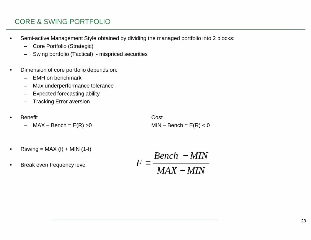
CORE & SWING PORTFOLIO

• Semi-active Management Style obtained by dividing the managed portfolio into 2 blocks:– Core Portfolio (Strategic)– Swing portfolio (Tactical) - mispriced securities

• Dimension of core portfolio depends on:– EMH on benchmark– Max underperformance tolerance– Expected forecasting ability– Tracking Error aversion

• Benefit Cost

23

• Benefit Cost– MAX – Bench = E(R) >0 MIN – Bench = E(R) < 0

• Rswing = MAX (f) + MIN (1-f)

• Break even frequency levelMINMAX

MINBenchF

−−

=

Government bonds

50%

Treasury bills30%

Large company

stock20%

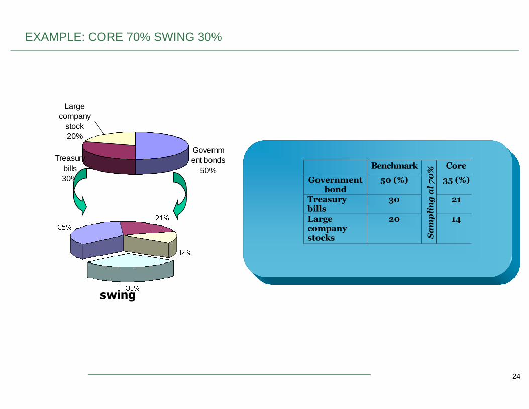
EXAMPLE: CORE 70% SWING 30%

Benchmark Core

Governmentbond

50 (%) 35 (%)

Treasurybills

30 21

Sampling al 70%

24

swing

bills

Largecompanystocks

20

Sampling al 70%

14

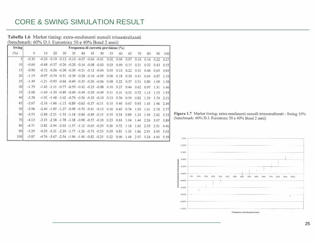
CORE & SWING SIMULATION RESULT

25

HOW DO YOU MEASURE THE RISK OF A PORTFOLIO?

• Absolute risk: Volatility of returns

• Relative risk: Volatility relative to a benchmark– Example: Tracking error or Active risk

• Active return = Portfolio return - Benchmark return

• Tracking error = standard deviation of active returns

– Application: Information ratio = alpha / tracking errori. (Alpha = average active return)

26

i. (Alpha = average active return)

• Estimation of tracking error:– Trailing active returns (backward looking estimate)– Risk model e.g., Barra (forward looking estimate)

A MEASURE OF RISK

• An important risk metric for portfolios that are managed versus a benchmark• Typical values:

– 0% for index funds– less than 2% for enhanced index funds– 5% for active large cap stock funds

• Number of stocks held - those in the benchmark and those not in the benchmark– Size or Style or Sector bets– Beta– Benchmark volatility

27

– Benchmark volatility

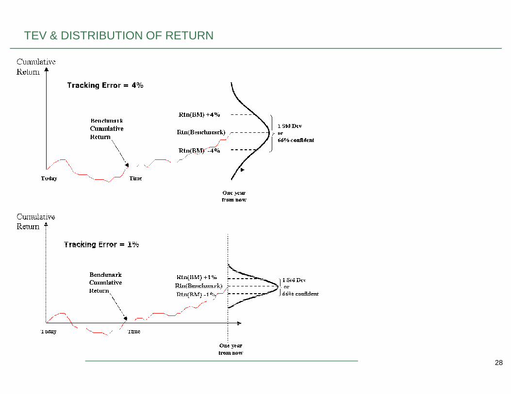
TEV & DISTRIBUTION OF RETURN

28

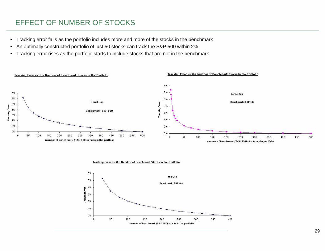
EFFECT OF NUMBER OF STOCKS

• Tracking error falls as the portfolio includes more and more of the stocks in the benchmark• An optimally constructed portfolio of just 50 stocks can track the S&P 500 within 2%• Tracking error rises as the portfolio starts to include stocks that are not in the benchmark

29

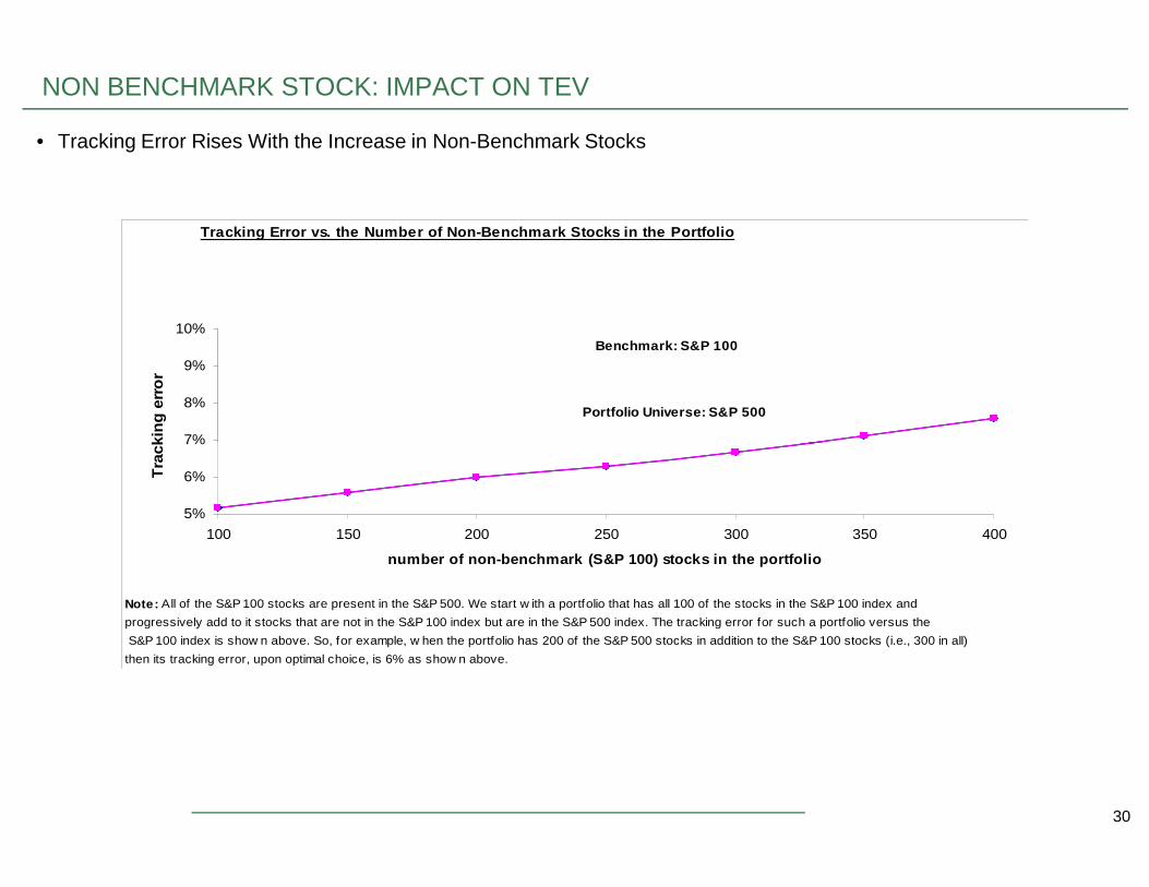
Tracking Error vs. the Number of Non-Benchmark Stoc ks in the Portfolio

7%

8%

9%

10%

Tra

ckin

g e

rro

r

Benchmark: S&P 100

Portfolio Universe: S&P 500

NON BENCHMARK STOCK: IMPACT ON TEV

• Tracking Error Rises With the Increase in Non-Benchmark Stocks

30

Note: All of the S&P 100 stocks are present in the S&P 500. We start w ith a portfolio that has all 100 of the stocks in the S&P 100 index and

progressively add to it stocks that are not in the S&P 100 index but are in the S&P 500 index. The tracking error for such a portfolio versus the

S&P 100 index is show n above. So, for example, w hen the portfolio has 200 of the S&P 500 stocks in addition to the S&P 100 stocks (i.e., 300 in all)

then its tracking error, upon optimal choice, is 6% as show n above.

5%

6%

7%

100 150 200 250 300 350 400

number of non-benchmark (S&P 100) stocks in the portfolio

Tra

ckin

g e

rro

r

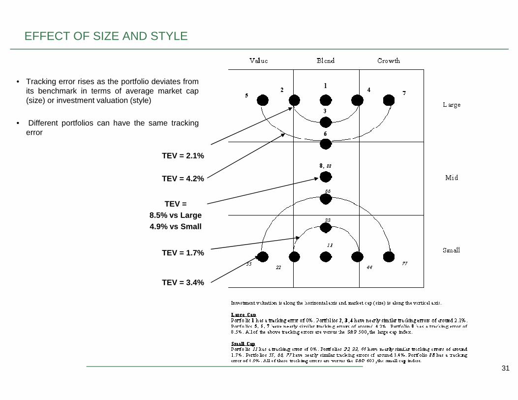
EFFECT OF SIZE AND STYLE

• Tracking error rises as the portfolio deviates fromits benchmark in terms of average market cap(size) or investment valuation (style)

• Different portfolios can have the same trackingerror

TEV = 2.1%

TEV = 4.2%

TEV =

31

TEV = 8.5% vs Large4.9% vs Small

TEV = 1.7%

TEV = 3.4%

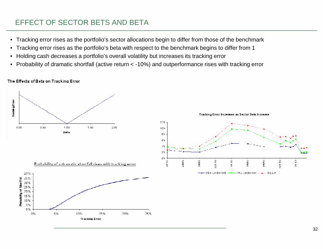
EFFECT OF SECTOR BETS AND BETA

• Tracking error rises as the portfolio’s sector allocations begin to differ from those of the benchmark• Tracking error rises as the portfolio’s beta with respect to the benchmark begins to differ from 1• Holding cash decreases a portfolio’s overall volatility but increases its tracking error• Probability of dramatic shortfall (active return < -10%) and outperformance rises with tracking error

32

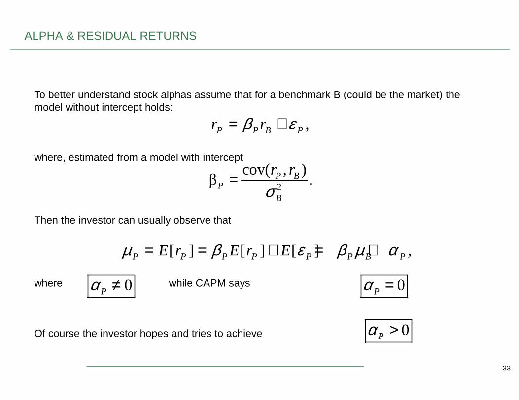
To better understand stock alphas assume that for a benchmark B (could be the market) the model without intercept holds:

where, estimated from a model with intercept

,P P B Pr rβ ε= +

2

cov( , )β .P B

PB

r r

σ=

ALPHA & RESIDUAL RETURNS

33

Then the investor can usually observe that

where while CAPM says

Of course the investor hopes and tries to achieve

Bσ

[ ] [ ] [ ] ,P P P P P P B PE r E r Eµ β ε β µ α= = + = +

0Pα ≠ 0Pα =

0Pα >

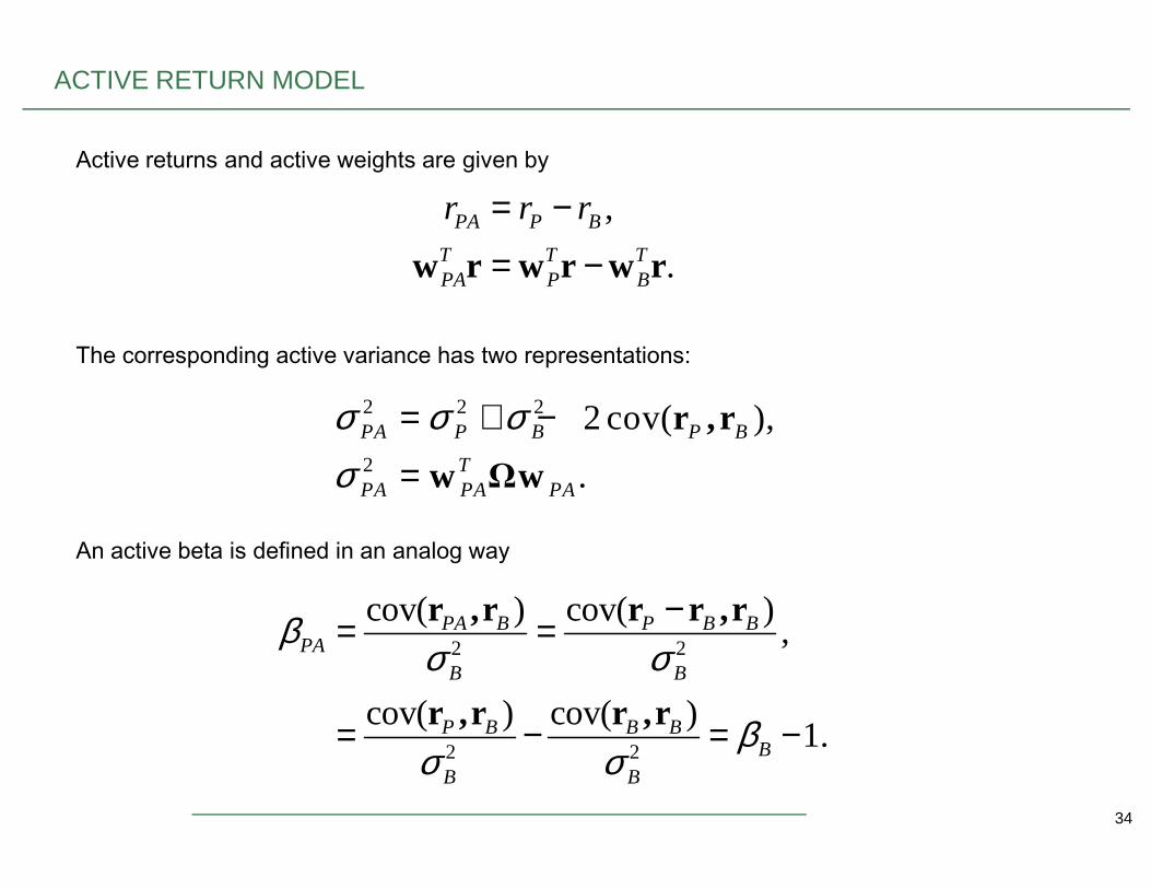
Active returns and active weights are given by

The corresponding active variance has two representations:

,

.PA P B

T T TPA P B

r r r= −

= −w r w r w r

2 2 2 2 cov( ),PA P B P Bσ σ σ= + − r , r

ACTIVE RETURN MODEL

34

An active beta is defined in an analog way

2 .TPA PA PAσ = w Ωw

2 2

2 2

cov( ) cov( ),

cov( ) cov( )1.

PA B P B BPA

B B

P B B BB

B B

βσ σ

βσ σ

−= =

= − = −

r ,r r r ,r

r ,r r ,r

The active returns model written in terms of active beta is

with active variance (TEV)

% ,PAPA PA Br rβ ε= +

2 2 2 2var( ) , since ( , ) 0.PA PA PA B B PAr corr rεσ β σ σ ε= = + =

ACTIVE RETURN MODEL

35

Note:

(1) Active variance is often called Tracking Error Variance (TEV)

(2) Performance of portfolio manager is measure by TEV (low=good)

(3) TEV is minimal, if active beta

(4) Since a portfolio beta of implies

(5) Usually managers avoid

0.PAβ =

1PA Pβ β= − 1Pβ = 0.PAβ =

1.Pβ >

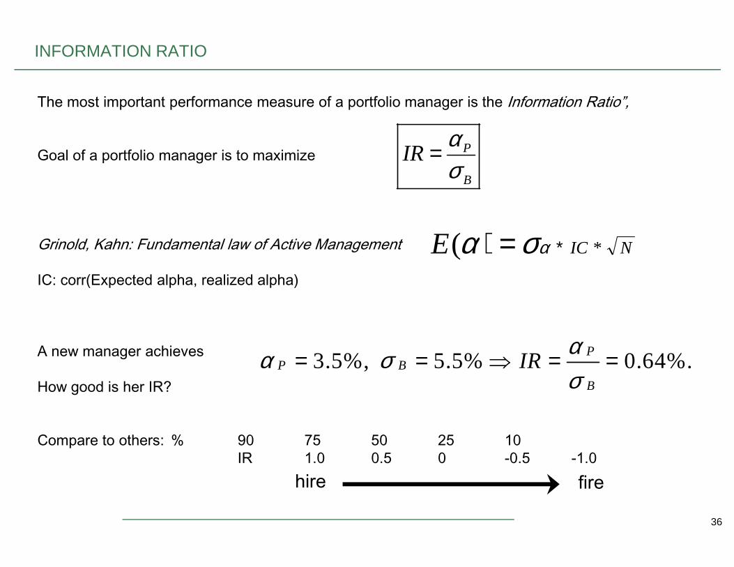
The most important performance measure of a portfolio manager is the Information Ratio”,

Goal of a portfolio manager is to maximize

Grinold, Kahn: Fundamental law of Active Management

IC: corr(Expected alpha, realized alpha)

P

B

IRασ

=

INFORMATION RATIO

NICE *( ∗=) ασα

36

IC: corr(Expected alpha, realized alpha)

A new manager achieves

How good is her IR?

Compare to others: % 90 75 50 25 10IR 1.0 0.5 0 -0.5 -1.0

3.5%, 5.5% 0.64%.

PP B

B

IRαα σσ

= = ⇒ = =

hire fire

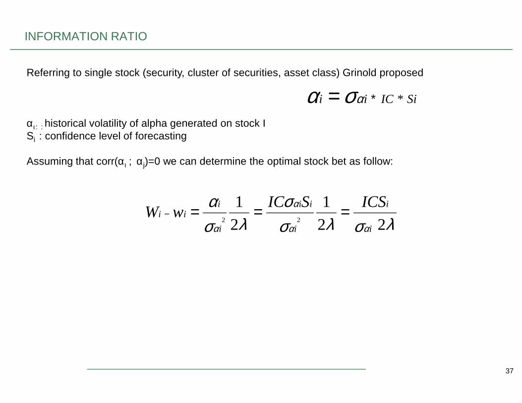
Referring to single stock (security, cluster of securities, asset class) Grinold proposed

αι: : historical volatility of alpha generated on stock ISi : confidence level of forecasting

Assuming that corr(αι ; αj)=0 we can determine the optimal stock bet as follow:

INFORMATION RATIO

SiICii *∗= ασα

σα α 11 iiii ICSSIC ===

37

λσλσσ

λσα

αα

α

α 22

1

2

122

i

i

i

ii

i

iii

ICSSICwW ===−

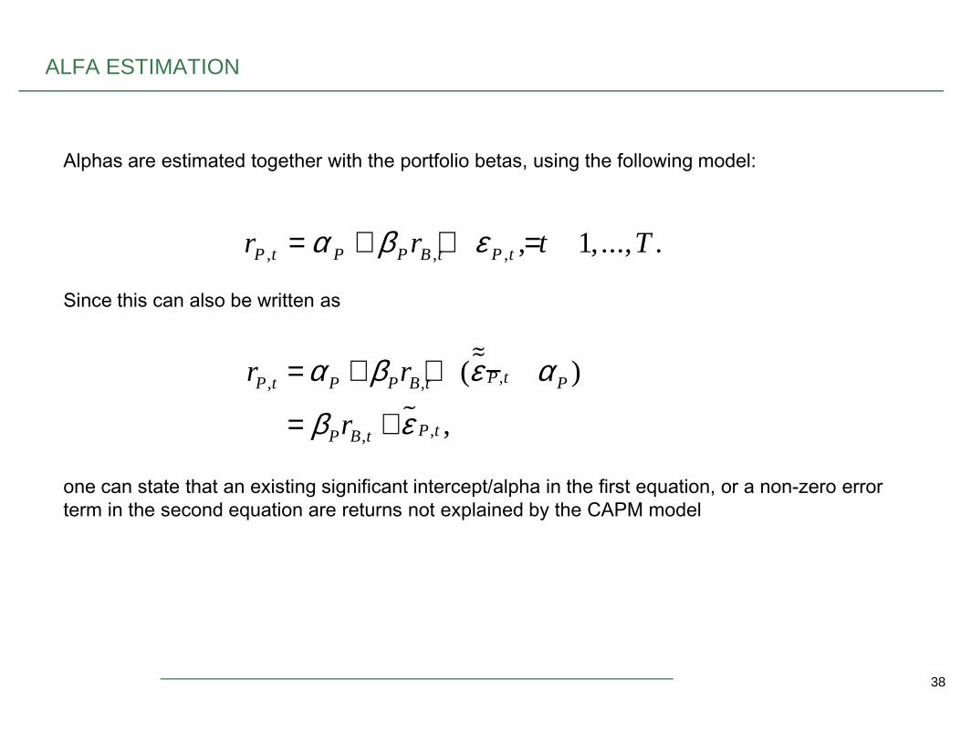
Alphas are estimated together with the portfolio betas, using the following model:

Since this can also be written as

, , , , 1,..., .P t P P B t P tr r t Tα β ε= + + =

%%,( )P tr rα β ε α= + + −

ALFA ESTIMATION

38

one can state that an existing significant intercept/alpha in the first equation, or a non-zero error term in the second equation are returns not explained by the CAPM model

%%

%

,, ,

,,

( )

,

P tP t P P B t P

P tP B t

r r

r

α β ε α

β ε

= + + −

= +

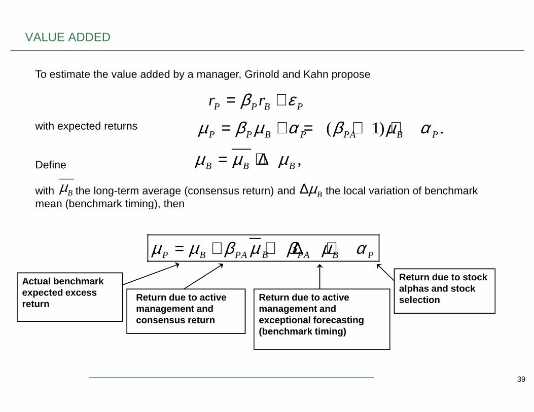
To estimate the value added by a manager, Grinold and Kahn propose

with expected returns

Define

with the long-term average (consensus return) and the local variation of benchmark mean (benchmark timing), then

P P B Pr rβ ε= +

( 1) .P P B P PA B Pµ β µ α β µ α= + = + +

Bµ

,B B Bµ µ µ= + ∆

Bµ∆

VALUE ADDED

39

mean (benchmark timing), then

BP B PA PA B Pµ µ β µ β µ α= + + ∆ +

Actual benchmark expected excess return

Return due to active management and consensus return

Return due to active management and exceptional forecasting (benchmark timing)

Return due to stock alphas and stock selection

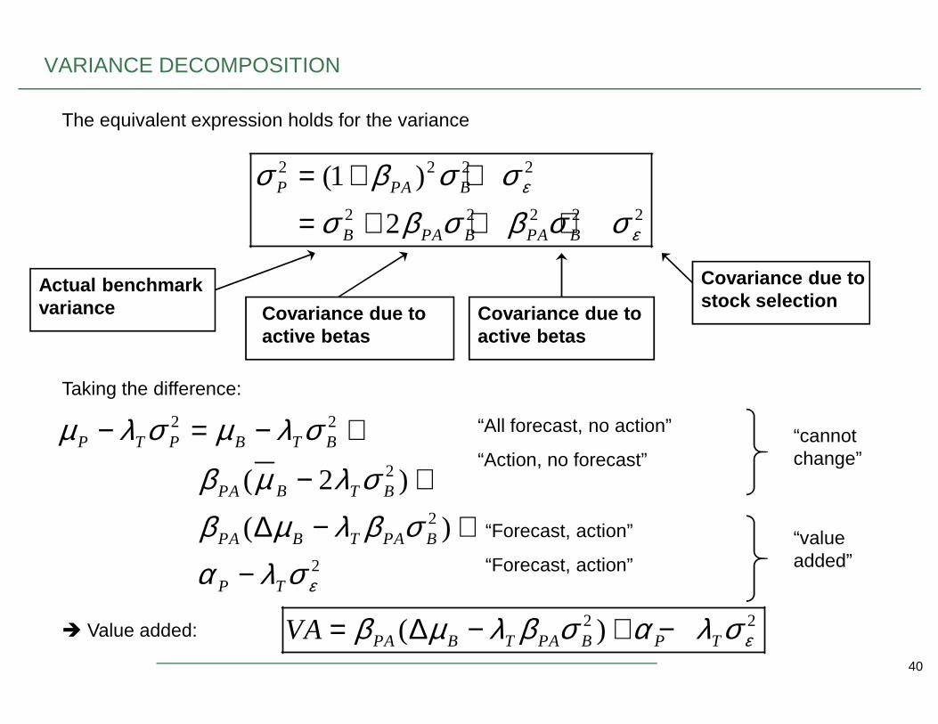
The equivalent expression holds for the variance

2 2 2 2

2 2 2 2 2

(1 )

2P PA B

B PA B PA B

ε

ε

σ β σ σσ β σ β σ σ

= + +

= + + +

Actual benchmark variance Covariance due to

active betasCovariance due to active betas

Covariance due to stock selection

VARIANCE DECOMPOSITION

40

Taking the difference:

2 2

2

2

2

( 2 )

( )

P T P B T B

BPA T B

PA B T PA B

P T ε

µ λ σ µ λ σβ µ λ σβ µ λ β σα λ σ

− = − +

− +

∆ − +

−

“All forecast, no action”

“Action, no forecast”

“Forecast, action”

“Forecast, action”“valueadded”

“cannot change”

2 2( )PA B T PA B P TVA εβ µ λ β σ α λ σ= ∆ − + − Value added:

APPENDIX

41

NOTION OF TRACKING ERROR

When managing an active investment portfolio against a well-defined benchmark (such as the Standard & Poor’s 500 or the IPSA index), the goal of the manager should be to generate a return that exceeds that of the benchmark while minimizing the portfolio’s return volatility relative to the benchmark. Said differently, the manager should try to maximize alpha while minimizing tracking error. Tracking error can be defined as the extent to which return fluctuations in the managed portfolio are not correlated with return fluctuations in the benchmark. The concept is analogous to the statistic (1 – R2) in a regression context. A flexible and straightforward way of measuring tracking error can be developed as follows:

42

Let: wi = investment weight of asset i in the managed portfolio Rit = return to asset i in period t Rbt = return to the benchmark portfolio in period t. With these definitions, we can define the period t return to managed portfolio as:

∑=

=N

iitR

1ipt w R

where: N = number of assets in the managed portfolio and:

1 w1

i =∑=

N

i

(i.e., the managed portfolio is fully invested).

NOTION OF TRACKING ERROR (CONT.)

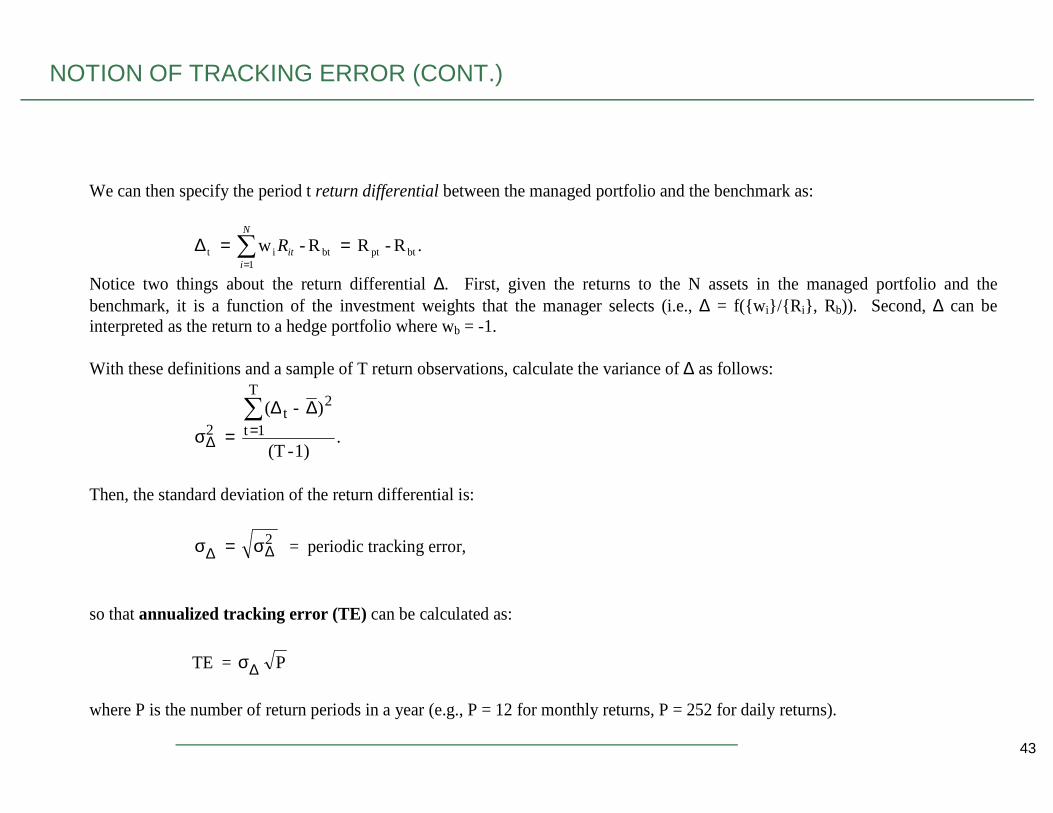
We can then specify the period t return differential between the managed portfolio and the benchmark as:

.R - R R - w btptbt1

it ==∆ ∑=

N

iitR

Notice two things about the return differential ∆. First, given the returns to the N assets in the managed portfolio and the benchmark, it is a function of the investment weights that the manager selects (i.e., ∆ = f(w i/R i, Rb)). Second, ∆ can be interpreted as the return to a hedge portfolio where wb = -1. With these definitions and a sample of T return observations, calculate the variance of ∆ as follows:

) - (T

2t∑ ∆∆

43

.1) - (T

) - (

1t

2t

2∑=

∆

∆∆=σ

Then, the standard deviation of the return differential is:

2 ∆∆ σ=σ = periodic tracking error,

so that annualized tracking error (TE) can be calculated as:

TE = P ∆σ

where P is the number of return periods in a year (e.g., P = 12 for monthly returns, P = 252 for daily returns).

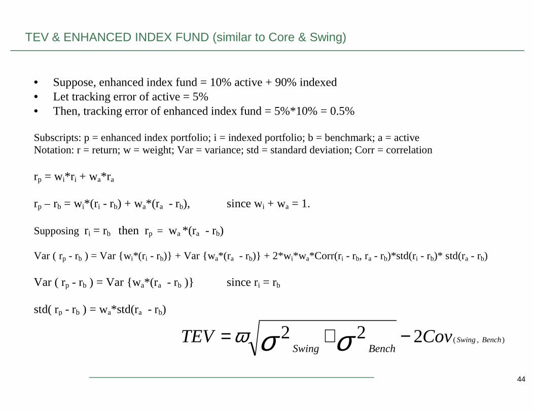
• Suppose, enhanced index fund = 10% active + 90% indexed • Let tracking error of active = 5% • Then, tracking error of enhanced index fund = 5%*10% = 0.5% Subscripts: p = enhanced index portfolio; i = indexed portfolio; b = benchmark; a = active Notation: r = return; w = weight; Var = variance; std = standard deviation; Corr = correlation rp = wi*r i + wa*r a rp – rb = wi*(r i - rb) + wa*(r a - rb), since wi + wa = 1.

TEV & ENHANCED INDEX FUND (similar to Core & Swing)

44

rp – rb = wi*(r i - rb) + wa*(r a - rb), since wi + wa = 1. Supposing ri = rb then rp = wa *(r a - rb) Var ( rp - rb ) = Var wi*(r i - rb) + Var wa*(r a - rb) + 2*w i*wa*Corr(ri - rb, ra - rb)*std(ri - rb)* std(ra - rb) Var ( rp - rb ) = Var wa*(r a - rb ) since ri = rb std( rp - rb ) = wa*std(ra - rb)

),(222 BenchSwingCovTEVBenchSwing

−+= σσω

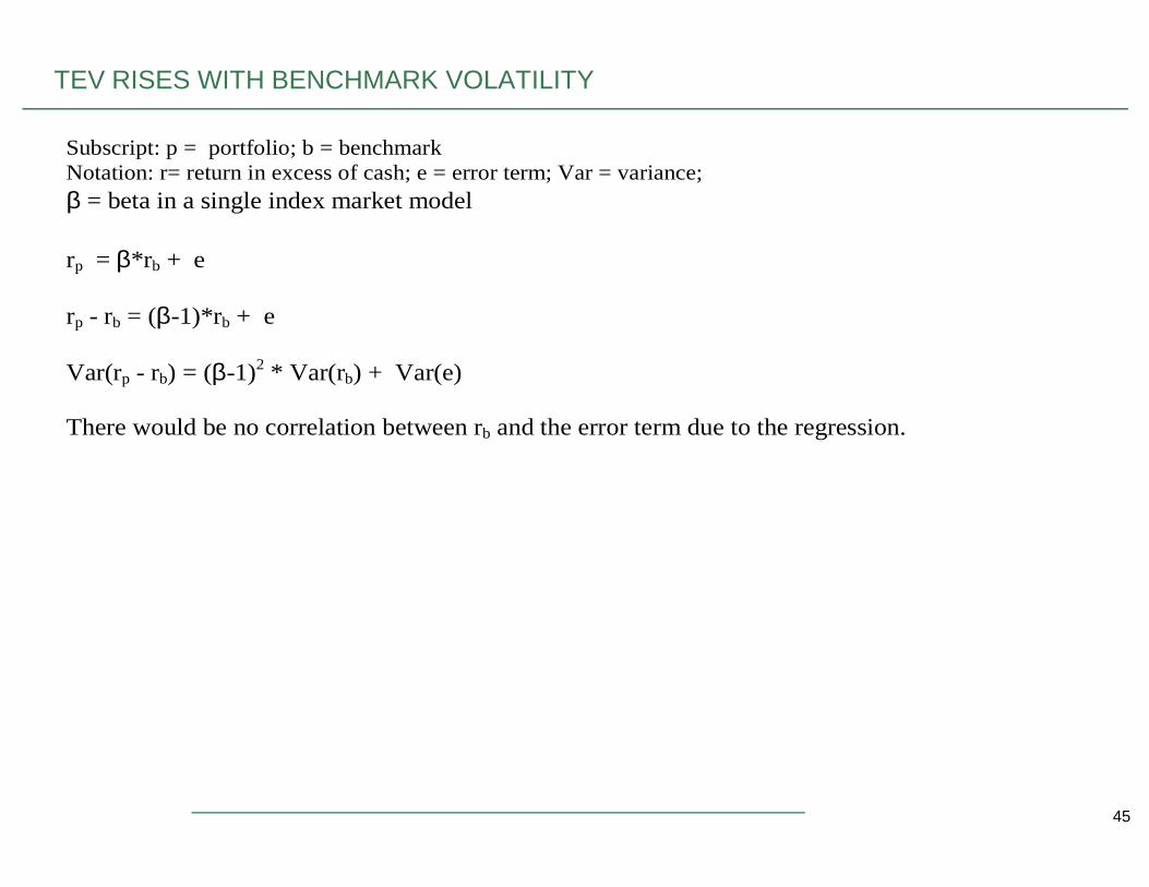
Subscript: p = portfolio; b = benchmark Notation: r= return in excess of cash; e = error term; Var = variance; β = beta in a single index market model rp = β*r b + e rp - rb = (β-1)*rb + e Var(rp - rb) = (β-1)2 * Var(rb) + Var(e) There would be no correlation between rb and the error term due to the regression.

TEV RISES WITH BENCHMARK VOLATILITY

45

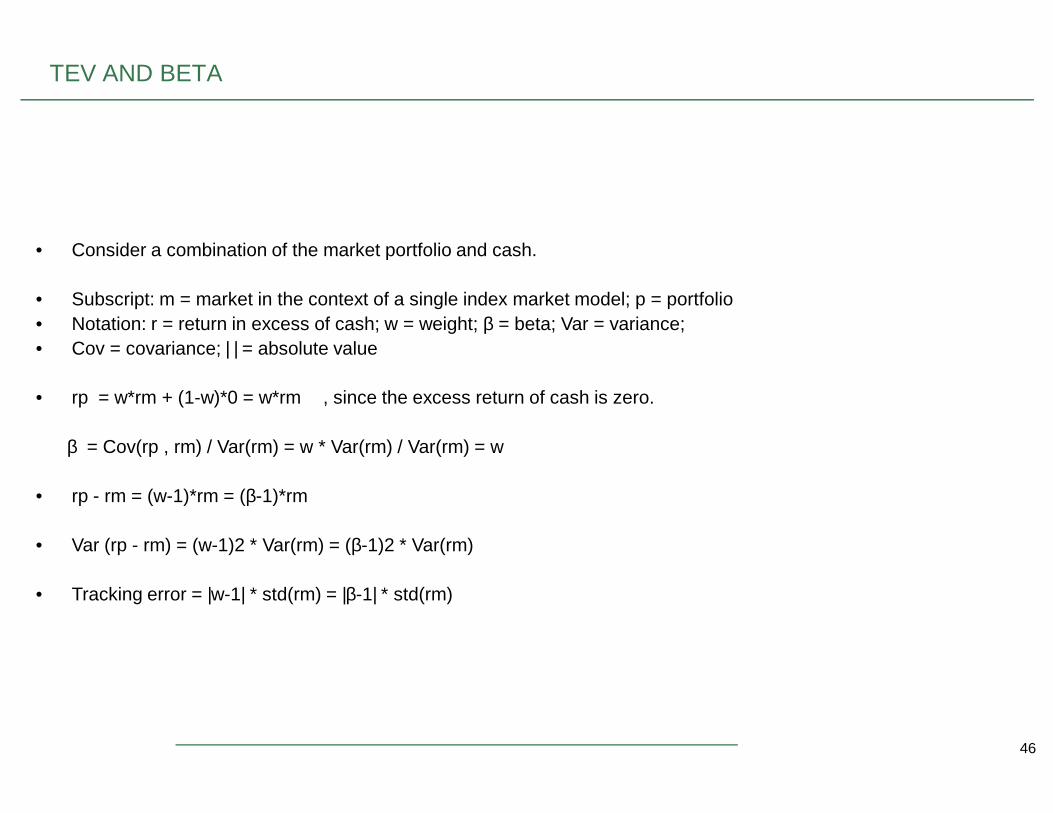
• Consider a combination of the market portfolio and cash.

• Subscript: m = market in the context of a single index market model; p = portfolio• Notation: r = return in excess of cash; w = weight; β = beta; Var = variance;• Cov = covariance; | | = absolute value

• rp = w*rm + (1-w)*0 = w*rm , since the excess return of cash is zero.

TEV AND BETA

46

• rp = w*rm + (1-w)*0 = w*rm , since the excess return of cash is zero.

β = Cov(rp , rm) / Var(rm) = w * Var(rm) / Var(rm) = w

• rp - rm = (w-1)*rm = (β-1)*rm

• Var (rp - rm) = (w-1)2 * Var(rm) = (β-1)2 * Var(rm)

• Tracking error = |w-1| * std(rm) = |β-1| * std(rm)