ECE 678 Introduction to BioMEMS Fall 2011 Final Report · PDF file1 ECE 678 Introduction to...
15
1 ECE 678 Introduction to BioMEMS Fall 2011 Final Report Group B Woohyuck Choi
Transcript of ECE 678 Introduction to BioMEMS Fall 2011 Final Report · PDF file1 ECE 678 Introduction to...

1
ECE 678 Introduction to BioMEMS
Fall 2011
Final Report
Group B
Woohyuck Choi

2
1. Introduction
Microfluidics is a growing field of study that has become a significant part of both research
and industry. A couple of primary benefits to microfluidic mixing are that it consumes small
amounts of valuable reagents and it mixes quickly. There are many applications for micromixers
that include: lab-on-a-chip devices, cover micro arrays, DNA sequencing, sample preparation
and analysis, cell separation and detection, and also environmental monitoring [1],[2]. Due to
this wide range of applications and many other potential applications, improving micromixers is
an important area of research.
Types of micromixers:
In general, there are two types of micromixers, active micromixers and passive micromixers.
Active Mircomixers:
The mixing process utilizes the disturbance generated by the external fields. External
disturbances like pressure, temperature, electrohydrodynamics, dielectrophoresis, electrokinetics,
magnetohydrodynamics and acoustics can be used in active mixers. The advantages of active
mixers are that mixing length is short, and they can be activated on demand. For the working of
active mixers, external power sources are required which makes the integration of mixers in a
microfluidic system challenging and expensive. Hence passive mixers are commonly used [2].
Passive Micromixers:
These mixers do not require an external energy source, and they totally rely on channel
geometry to increase vorticity and cause mixing. The types of passive mixers are: parallel
lamination, serial lamination, injection, chaotic advection and droplet. The advantages of using
passive mixers are that fabrication is simple, cost is low and they are less likely to damage
biological samples. However, passive micromixers require longer mixing lengths and have
longer mixing times than their active counterpart [2].
Methods of Mixing in Passive Micromixers:
There are two primary methods of mixing in passive micromixers which are molecular
diffusion based and chaotic advection based [2]. Increasing the contact area of the two fluids in
the channel and decreasing the diffusion path are the ways to improve molecular diffusion based
mixing [2]. Two primary methods to decrease the diffusion path are making narrow channels and
using hydrodynamic focusing. Hydrodynamic focusing is where a fluid is introduced tangential
to the initial fluid in the channel such that the width of the initial fluid is decreased [3]. Chaotic
advection involves manipulating the laminar flow in a channel such that one is forcing fluids
across their natural boundary in the channel [2]. The simplest way to achieve this is by adding
specific 3-D obstacles to the channel [2].

3
2. Design and Modeling
Purpose:
The purpose of this module is to optimize the performance of a microfluidic mixer by
changing the dimensions of the channel. The objective is to obtain the highest percent mixing,
which means the lowest σ value, while keeping the pressure drop of the entire channel below
1Kpa/mm.
Introduction:
Previous to this exercise our group has already decided on a basic design for our channel.
We have also identified three variables with five different values for each variable which we will
manipulate in order to attempt to optimize our mixer. An image of a single unit of our mixer can
be seen in Figure 1 and a table of the optimization variables can be seen in Table 1.
Figure 1: One unit of the “serpent” mixer Table 1: A list of the different values for optimization.
showing the three variables we Five distinct levels were chosen for each
altered. variable. The initial values set for each variable
are highlighted in red.
The values for optimization were chosen based on one initial experiment that was run using the
initial values denoted in Table 1. The model was run in CFD-ACE+ in two dimensions instead of
three in order to be able to use a finer, more accurate, mesh and to lower simulation times. The
model was run with a 3um triangular mesh for Re=1. The results of this simulation at the outlet,
4910um, were 92.83 percent mixing and a pressure drop of 6569Pa. The pressure drop was too
high (greater than 1KPa/mm) thus we knew we needed to lower the pressure drop of our channel.
We knew that increasing the dimensions of the channel would lower the pressure drop. This is
why most of the optimization values chosen are larger than the initial values.
Procedure:
The method that we chose in order to best optimize our channel is to change one variable
at a time and optimize that variable. Then for the second variable we set the first variable to its
optimized value, and optimized for the second variable and so on. We felt that this would give us
good optimization without having to run too many models, as one would have to do in factorial
optimization.
Level 1 Level 2 Level 3 Level 4 Level 5 Level 6
Variable 1 30um 35um 40um 45um 50um --------
Variable 2 25um 30um 35um 40um 45um 50um
Variable 3 25um 30um 32um 35um 38um 40um
4
For all optimization we ran the models in CFD-ACE+ in two dimensions for the same
reasons as previously stated. All of the models were run with a 3um triangular mesh and for
Re=1. The values assigned to the simulator before each run can be seen in Table 2.
CFD-ACD+
Variable Value Assigned
Reference Pressure 100,000 Pa
Liquid Mixing Rule Water
Density (ρ) 1,000 kg/m^3
Viscosity (μ) .001 kg/m-s
Diffusivity 1E-10 m^2/s
X-Direction
Velocity
.00125 m/s (Re=.1)
.0125 m/s (Re=1)
.125 m/s (Re=10)
Dye 1 Molar Concentration in Water
No Dye 0 Molar Concentration in Water
Temperature 300K
Iterations 1500
Convergence
Criteria 1.00E-06
Minimum Residual 1.00E-18
Differencing:
Velocity Upwind
Species 2nd Order Limiter with .01 Blending
Solvers:
Velocity CGS + Pre (500 sweeps, .0001
criterion)
P Correction AMG (50 sweeps, .1 criterion)
Species CGS + Pre (500 sweeps, .0001
criterion)
Table 2: Values assigned in the CFD-ACE+ Simulator
The equation for calculating percent mixing is: %𝑚𝑖𝑥𝑖𝑛𝑔 = (1− 𝐴𝑣𝑒𝑟𝑎𝑔𝑒1 − 𝐴𝑣𝑒𝑟𝑎𝑔𝑒2 ) ×100 where Average 1 is the average molar concentration of the top half of the channel, and
Average 2 is the average molar concentration of the bottom half. The equation used to calculate
σ is:σ =(100−%𝑚𝑖𝑥𝑖𝑛𝑔 )
100×
1
2. Also the values of the pressure drop of the entire channel, and
vorticity in the channel are investigated in CFD-View.
Once we had all of the optimization data we decided to compare our mixer to a straight
“T-Mixer” of approximately the same dimensions and effective mixing length of our “serpent”
mixer. Doing this would allow us to see how well our mixer performed compared to a strictly
diffusive mixer. The dimensions of the “T-Mixer” were 40um wide and 17519um long. The
simulation was run in two dimensions with a 3micron triangular mesh for Re=1.
The X-Direction velocities were
calculated for the Reynold’s numbers of
0.1, 1, and 10 using the equation for
Reynold’s number: 𝑅𝑒 =𝜌𝑣𝐷
𝜇. This
equation is then solved for velocity:
𝑣 =𝑅𝑒𝜇
𝜌𝐷. All of the values are known
except D which is the hydraulic diameter.
The equation for hydraulic diameter is :
𝐷 =4𝐴
𝑈 where A is the area of the channel
and U is the wetted perimeter. For our
200um square inlet D=80microns. After
each simulation is run the results of the
simulation are imported into CFD-View.
In this program x-cuts are made at certain
positions along the channel and the
H20_Molar concentration at each of these
x-cuts are plotted. The x-cuts that we
made in our channel are at the following
lengths along the channel: 0um, 750um.
1790um, 2830um, 3870um, 4910um.
These values were chosen such that the
cuts would be made in the same area of
each unit. The data from these plots is
then exported to MS Excel where percent
mixing and σ can be calculated.

5
After we were done with optimization the fully optimized channel was extruded in three
dimensions such that it would be 50um deep. This three dimensional model was then meshed
using a 5um triangular mesh. We attempted to use the 3um triangular mesh for the three
dimensional models since we had used this meshing for the two dimensional ones; however, the
simulator reported a memory error due to the fact that the 3um meshing created too many cells in
the three dimensional channel. The smallest meshing size we could use that did not report an
error was 5um, thus we selected this value. For the optimized three dimensional models we ran
simulations for three different Reynolds numbers: 0.1, 1, and 10. The results of these simulations
were imported into CFD-View and the %mixing, σ, pressure drop, and vorticity for the channel
were obtained in the same fashion as they were for the two dimensional models.
Results:
Optimization:
The results for the optimization of variable 1 can be seen in Figure 2 below. A table of
the values obtained can be seen in Table 3. For this optimization variable 2 and variable 3 were
set to be 30um while variable 1 was adjusted.
For this variable we chose 40um as our optimized value due to the fact that is achieved the
highest percent mixing while being below the 5KPa limit.
For variable 2 we set variable 1 to be 40um and variable 3 to be 30um and varied variable
2. Figure 3 shows the graphical results of this optimization and Table 4 shows the values.
0
0.1
0.2
0.3
0.4
0.5
30um 35um 40um 45um 50um
σ
Variable Value
σ for Variable 1 at Outlet
0
0.1
0.2
0.3
0.4
0.5
25um 30um 35um 40um 45um 50um
σ
Variable Value
σ for Variable 2 at Outlet
Variable Value
Percent Mixing σ
Pressure Drop (Pa)
30um 92.83 0.035865 6569
35um 91.16 0.044183 5634
40um 89.07 0.054644 4989
45um 87.01 0.064927 4536
50um 85.48 0.072621 4180
Variable Value
Percent Mixing σ
Pressure Drop (Pa)
25um 89.84 0.050798 5449
30um 89.07 0.054644 4989
35um 87.78 0.061084 4712
40um 86.72 0.066408 4523
45um 86.66 0.066713 4390
50um 86.73 0.066375 4302
Figure 2: A plot of σ vs. variable value for variable 1.
All values are taken at the outlet (4910um)
Table 3: Values used in Figure 2. The value in red is
the selected value for optimization.
Figure 3: A plot of σ vs. variable value for variable 2.
All values are taken at the outlet (4910um) Table 4: Values used in Figure 3. The value in red is
the selected value for optimization.

6
We chose 30um as the optimized value for this variable since it had the highest percent mixing
while also fulfilling the pressure requirement.
For variable 3 we set variable 1 to be 40um and variable 2 to be 30um and varied variable
3. The graphical results of this optimization can be seen in Figure 4. A table of the values is
given in Table 5.
We chose 30um as the optimized value for variable 3 due to the highest percent mixing while
remaining below the pressure drop cap.
T-Mixer:
The results at the outlet of the “T-Mixer” were: 91.4% mixing and 8333Pa pressure drop.
Optimized Serpent Mixer:
Now that we had all of the levels for all of the variables we made our optimized mixer.
An image showing all of the dimensions of a single unit of the optimized mixer can be seen in
Figure 5.
Figure 5: Dimensions of optimized channel. All numbers shown are in microns
0
0.1
0.2
0.3
0.4
0.5
25um 30um 32um 35um 38um 40um
σ
Variable Values
σ for Variable 3 at OutletVariable
Value Percent Mixing σ
Pressure Drop (Pa)
25um 89.54 0.05231 5100
30um 89.07 0.054651 4990
32um 88.60 0.056992 4882
35um 88.13 0.059333 4802
38um 87.43 0.062871 4724
40um 86.80 0.065992 4683
Figure 4: A plot of σ vs. variable value for variable 3.
All values are taken at the outlet (4910um)
Table 5: Values used in Figure 4. The value in red is
the selected value for optimization.

7
The graphical results the optimized channel under the Re=.1 conditions can be seen in
Figure 6. Table 6 shows the values obtained from this simulation.
The results of the optimized channel under the Re=1 condition are graphed in Figure 7
and shown in Table 7.
The results of the optimized channel under the Re=10 condition are graphed in Figure 8 and
shown in Table 8.
0
0.1
0.2
0.3
0.4
0.5
0 750 1790 2830 3870 4910
σ
Downstream Position (um)
0
0.1
0.2
0.3
0.4
0.5
0 750 1790 2830 3870
σ
Downstream Position (um)
0
0.1
0.2
0.3
0.4
0.5
0 750 1790 2830 3870 4910
σ
Downstream Position (um(
Downstream Position
Percent Mixing σ
Pressure Drop (Pa)
0um 3.26 0.48369
1053
750um 51.61 0.241956
1790um 85.20 0.073986
2830um 95.51 0.022429
3870um 98.56 0.007187
4910um 99.58 0.002108
Downstream Position
Percent Mixing σ
Pressure Drop (Pa)
0um 3.17 0.484164
10700
750um 47.44 0.262803
1790um 77.55 0.112261
2830um 90.27 0.048634
3870um 95.81 0.02093
4910um 98.37 0.008168
Downstream Position
Percent Mixing σ
Pressure Drop (Pa)
0um 3.20 0.484011
130,800
750um 64.27 0.178647
1790um 93.13 0.034345
2830um 98.22 0.008909
3870um 99.52 0.002396
4910um 99.90 0.000504
σ vs. Downstream Position Re=.1
σ vs. Downstream Position Re=1
σ vs. Downstream Position Re=10
Figure 6: Graphical results of σ vs. channel length
for Re=0.1
Table 6: Values used in Figure 6.
Figure 7: Graphical results of σ vs. channel length
for Re=1
Table 7: Values used in Figure 7.
Figure 8: Graphical results of σ vs. channel length
for Re=10.
Table 8: Values used in Figure 8.

8
Discussion:
There are quite a few interesting aspects of our channel that we learned by going through
this optimization process. The fist aspect to note is that as we constricted the individual
dimensions of the channel the percent mixing always increased, but so did the pressure drop.
This is what we expected due to the fact that constricting the dimensions lowered the width over
which diffusion could take place. Due to the fact that there was a maximum pressure drop of
1KPa/mm we could only constrict these dimensions so far. In order to fully optimize the channel
we chose each variable such that it was the smallest possible while still following the pressure
drop guidelines.
When the channels were extruded in three dimensions a couple of issues arose. The first
issue was that we could not use the same size meshing as we had for optimization. By having to
use a larger meshing the simulator overestimated the mixing in the channel. This is why the
values for the three dimensional models are larger than the two dimensional ones. The other
issue was that the pressure in the channel approximately doubled for the three dimensional
models. Since we had optimized for the highest percent mixing, which was also the highest
allowed pressure, in two dimensions this doubling of the pressure put us well over the pressure
limit. We were unaware that this was going to happen, and did not have sufficient time to correct
the pressure drop.
Comparing our mixer to the “T-Mixer” also provided some interesting findings. When
compared to the “T-Mixer” our “serpent” mixer was worse by 2.33% mixing but had 3343Pa
lower pressure drop. One possible reason for the lower mixing performance is that the “serpent”
mixer is not 40um all the way through the channel. It varies from 40um to 65um in each diffuser
with 30um connections between diffusers. The overall effect of this is that we sacrifice a small
amount of mixing for a significant lowering of the pressure drop. Since our mixer performed
very closely to the “T-Mixer” we modeled it suggests that our mixer is primarily a diffusive
mixer. This also makes sense from the standpoint that there were no obstacles in the channel that
would cause a split and recombination of the flow.
The results from the three dimensional model with the three different Reynolds numbers
also told us a little bit about the mixing that was occurring in the channel. The Re= 0.1 case
provided greater mixing than the Re=1 case. This further supports the idea that the mixer is
primarily diffusive in nature since we achieved better mixing for a less turbulent flow. However,
the Re=10 case had better mixing than either of the other two cases. This may be due to the fact
that for large Reynolds numbers there may be a race track effect around the corners in our
channel. However, due to the large meshing of these three dimensional models the data from
these simulations is not very accurate.
Conclusion:
The “serpent” mixer design that was simulated is a primarily diffusive mixer. However,
due to the sharp bends in the channel there is some race track effect that is occurring that
becomes more pronounced at large Reynolds numbers. According to the simulation we expect to
obtain approximately 89% mixing in our channel for the Re=1 case. This number should increase
slightly for the Re=0.1 and Re=10 cases. However, the simulator also reported that we are going
to have high pressure drops which may cause the PDMS channels to rip and or the fluid to come
out of the channel. Also due to some inherent error in the simulator and the fact that the
dimensions obtained after fabrication will not be exactly what they were when we ran the
simulator we expect to see a drop in the percent mixing when the device is actually tested.

9
3. Fabrication of Device
Mask layout in AutoCAD:
AutoCAD was used to design the mask of our mixer using the dimensions from the final
design. This AutoCAD design was then sent out for fabrication of mask. For a 3” diameter wafer
we will require a 4” square mask. SU-8 is a negative photoresist and thus to get a negative of the
AutoCAD layout we will use a dark field chrome mask.
SU-8 Master Fabrication:
SU-8 master was fabricated for PDMS casting. MicroChem’s SU-8 resist was used on a
3” silicon wafer. The substrate was cleaned with an Acetone/methanol/DI water rinse followed
by a piranha clean. Then the wafer was dehydrated for 10 min at 150oC on a hotplate. A layer of
SU-8 was spin coated with a thickness of ~50 μm. A soft bake was done, using a leveled hot
plate, at 65oC for 5 min and ramped to 95
oC for 45 min, and then was allowed to cool down to
room temperature. The exposure was done using the mercury I-line (365 nm) high pass filter at
exposure energy of 175 mJ/cm2, for 35 sec. A glycerin layer was used in between the SU-8 wafer
and mask to reduce diffraction effects. Now, a post exposure bake was done which is similar to
the soft bake. MicroChem SU-8 developer was used to develop away the unexposed resist. The
wafer was developed for 2 hrs and then an IPA rinse was performed to confirm the completion of
development process. An O2 plasma etch was then performed to etch away a small layer from the
top of the SU-8. The final wafer obtained was free of cracks and non uniformities.
PDMS Casting:
SU-8 patterned wafers were coated with Sigmacote and left to air-dry for 30 min to
facilitate mold release. Next the PDMS was mixed at a 10:1 (m/m) ratio of elastomer base to
curing agent. PDMS must be mixed until it becomes milky-white due to the air bubbles stirred in
it. Degassing of PDMS component mixture is necessary for the removal of air bubbles, which
may degrade quality of the replication. Degassing was done by using a vacuum desiccator for 15
min. Then the PDMS was poured over the patterns directly, with care taken to avoid formation of
additional air bubbles. Again a process of degassing was done to remove any air bubbles formed
while transferring PDMS. The degassed PDMS was then cured using a hotplate at 80oC for 2hrs.
The curing time is dependent on the thickness of PDMS and the curing temperature. Finally, the
cast and cured PDMS is slowly peeled away from the mold, taking care not to damage the SU-8
master.
Bonding:
Bonding with oxygen plasma is one of the best ways to bond PDMS substrate with glass.
We used a corona discharge wand which ionizes air to treat PDMS surface. Inlet and outlet holes
were made by piercing a 14 gauge syringe tip in the final mixer cast at the points of the two fluid
inlets and the single outlet, respectively. Piranha clean was performed to clean the microscope
glass slides and then it was rinsed with DI water and then dried with nitrogen gas. The PDMS
casting was also washed using DI water. With the bonding side up, the clean glass slide and the
PDMS sample were placed on a non-conducting surface. The wire electrode was moved back
and forth approximately ¼ inches above the bonding surface for 20 sec. Finally the treated
surface was pressed together and left undisturbed for 2 hrs for complete bonding to take place.

10
4. Device Characterization
Structural Characterization:
The device was characterized under a microscope prior to plasma bonding. The channel
dimensions were recorded by placing the PDMS microchannel under the microscope. Figure 9
shows some of the photographs taken. It can be seen that the fabricated mixer is almost identical
to the designed mixer. There is only a few microns variation present in the final fabricated mixer
as compared to the designed one. The sharp corners turned out to be rounded as anticipated, due
to the non precise photolithography and SU-8 fabrication while working at small dimensions of
the order of 20 µm.
A ~1mm sliced cross section of the mixer along the z direction was used to observe and
characterize the channel cross-sectional features. The total height of the PDMS cast mixer
channel is shown in figure 9(B). It was measured to be 50.1 microns, which was only 0.1
microns larger than expected. This shows the accuracy of the recipe chosen to make the PDMS
molds. Figure 9(C) displays the fabrication of the PDMS microchannel at the regions of the
optimization variables chosen for the design. For variable one the dimensions are 40.1 microns
which is an increase by only 0.1 microns from the actual designed dimension. For variable two
the measured dimension was 33.54 microns which is more by 3.54 microns compared to the
actual design. Finally, for the third variable we got the fabricated dimensions as 30.31 microns
which is again just 0.31 microns larger than the actual design. These are very minor changes
occurring from designed micromixer to the fabricated one. This again shows the accuracy of the
SU-8 master fabrication and the PDMS casting process.
Figure 9:
(A) Channel top view
(B) Cross-sectional view of channel
wall
(C) View of the variables that were
optimized.

11
Overall, the casting shows little deviation in the dimensions from the CAD designs. Channel
dimensions differed from the AutoCAD and the CFD-GEOM designs mainly due to variations in
the exposure, etching, and casting procedures.
Fluid Flow Characterization:
The mixing characteristics of the micromixer were measured using a fluorescence dye.
During testing, a syringe pump was used to deliver water to one inlet and the dye solution to the
other. For the Reynolds number equal to 1, the flow rate was calculated to be 3.75 µL/min.
Images of mixing for Re=1 are shown in figure 10. The entrance image shows the difference
between Fluorescein and water. With changes in the intensity of the two liquids, as we proceed
along the channel length, progressive mixing can be calculated. 100% mixing is achieved when
the channel appears to only have one bright fluid in it. ImageJ was used to analyze the images for
percent mixing. Intensity values at each pixel were plotted versus the width of the channel. The
data for the channel was then extracted from these plots and was used to calculate percent mixing
and σ.
Figure 10: Images of subsequent mixing through channel. At 15.8 mm we can see that ~100% mixing has occurred.

12
Results and Discussion:
After fabricating the micromixer and finding out the new dimensions of the
microchannel, a new CFD-GEOM file was created with the dimensions of the final device. This
was done to compare the results obtained for the simulations run using the CFD tools and the
actual device. The conditions for this simulation were the same as before, but the mesh size used
in this case was 2 microns in order to get accurate results and save time.
At ~5 mm channel length the mixing percentage calculated from the simulated model and
the experimental data is shown in table 9.
Re=.1 Re=1 Re=10
Simulated %Mixing (2um mesh) 95.32 73.70 71.40
Experimental %Mixing 77.10 72.03 79.80
Difference 18.22 1.67 -8.40
Table 9: Comparison of % Mixing At 4910um Downstream
As seen from the table, the results from simulation and experiment for Re=1 are almost
matching. Whereas for the case of Re=0.1 the simulation results show an exaggerated percent
mixing. This error can be possibly accounted for the inaccurate simulation mathematics or
meshing layout. One unexpected result of the simulation was the percent mixing for the Re=10
case was the lowest of the three Reynolds numbers tested. In previous simulations and the
experimental results, the Re=10 case actually had a higher percent mixing than the Re=1 case.
Even though this was an unexpected and experimentally unverified result, the difference between
the simulator and the experimental data was still only 8.4% which is within acceptable range.
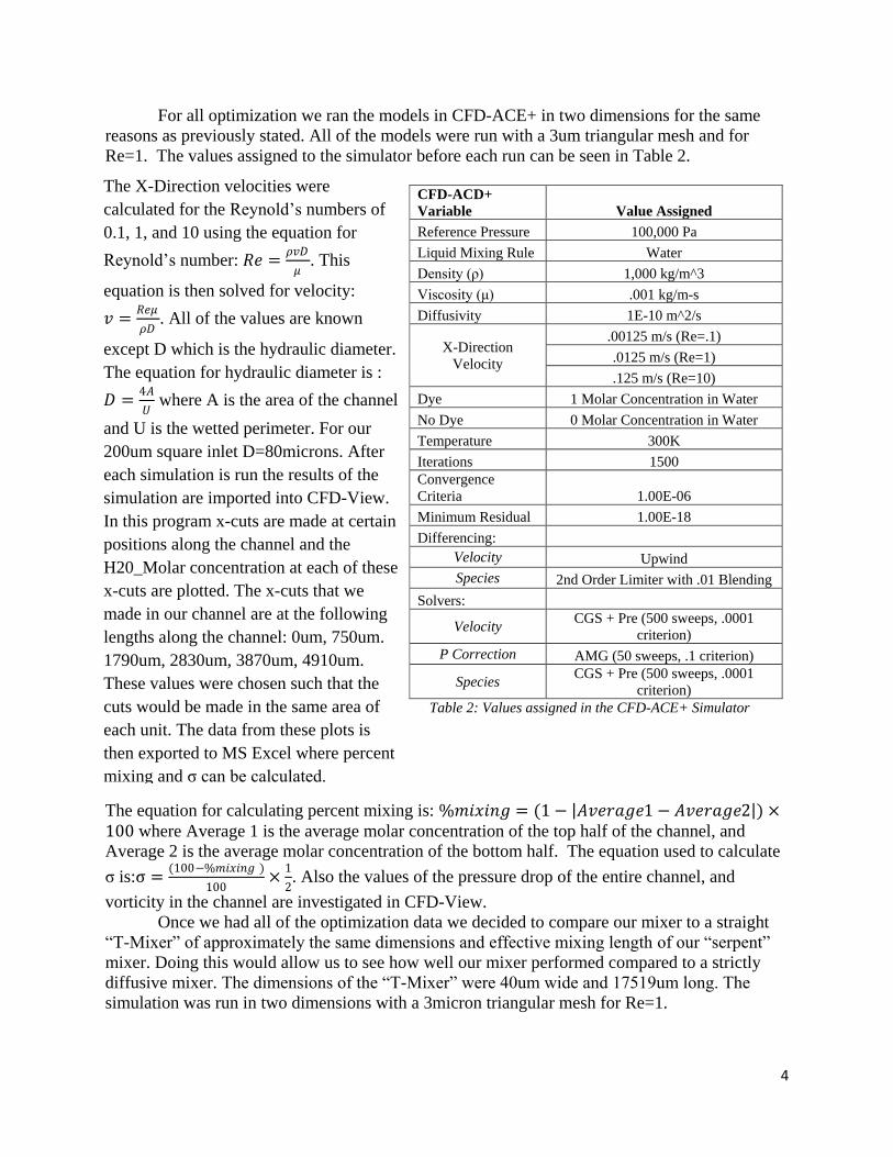
Figure 11 shows the graph for σ vs. downstream position for different Reynolds numbers.
Also figure 12 displays the variation in the value of σ with change in Reynolds number. It can be
seen that the mixing performance is worst for Re=1 whereas we get good mixing for Re=0.1 and
10. Good mixing at low Reynolds number is due to high amount of diffusivity between two
fluids. Also for Re=10 we get good mixing because of the race track effect present at the
curvatures as shown in Figure 13. Table 10 shows the comparison of the mixer for different
Reynolds numbers at different positions along the channel length. It also displays the y (90) for
the three cases i.e. the channel length at which the mixing percent reaches 90% and σ=0.05. The
y(90) was calculated for each channel by fitting a 4th
order polynomial to each curve and solving
this polynomial for σ=0.05.
13
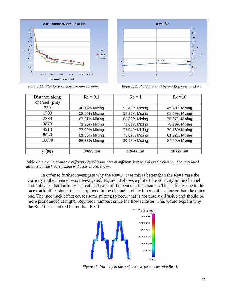
In order to further investigate why the Re=10 case mixes better than the Re=1 case the
vorticity in the channel was investigated. Figure 13 shows a plot of the vorticity in the channel
and indicates that vorticity is created at each of the bends in the channel. This is likely due to the
race track effect since it is a sharp bend in the channel and the inner path is shorter than the outer
one. The race track effect causes some mixing to occur that is not purely diffusive and should be
more pronounced at higher Reynolds numbers since the flow is faster. This would explain why
the Re=10 case mixed better than Re=1.
Figure 13: Vorticity in the optimized serpent mixer with Re=1.
Distance along
channel (µm)
Re = 0.1 Re = 1 Re =10
750 48.14% Mixing 53.40% Mixing 45.40% Mixing
1790 52.55% Mixing 58.22% Mixing 63.59% Mixing
2830 67.21% Mixing 63.39% Mixing 75.97% Mixing
3870 71.30% Mixing 71.61% Mixing 78.39% Mixing
4910 77.09% Mixing 72.04% Mixing 79.78% Mixing
8030 81.25% Mixing 75.82% Mixing 81.92% Mixing
10630 86.55% Mixing 80.73% Mixing 84.49% Mixing
y (90) 10895 µm 12642 µm 10729 µm
Figure 12: Plot for σ vs. different Reynolds numbers
Figure 11: Plot for σ vs. downstream position
Table 10: Percent mixing for different Reynolds numbers at different distances along the channel. The calculated
distance at which 90% mixing will occur is also shown.
Figure 11: Plot for σ vs. downstream position

14
5. Conclusion
The “serpent” mixer was initially designed and tested using the CFD software in order to
see what the expected performance of the channel would be. From these simulations we
discovered that we would achieve approximately 89 percent mixing at five millimeters into the
channel for Re=1 and a pressure drop of approximately 10.7 KPa. Due to meshing constraints,
inherent error in the simulation software, and potential deviation in dimensions due to fabrication
we expected that the actual performance of our mixer would be lower by up to 20 percent.
The SU-8 master fabrication and PDMS casting techniques were very precise. The
fabricated model only deviated from the mask dimensions by a few microns. It was also noticed
that the sharp corners in the device got rounded slightly. Neither of these issues will cause a
significant deviation from the simulated mixer results.
Once the exact dimensions of the fabricated channel were known the geometry file was
changed to match these dimensions and simulated again. The results of this simulation were
compared with the actual experimental data and it was found that there was a maximum
deviation of approximately 18 percent from simulated to experimental data which is close to
what we estimated the difference would be. For the experimental results at 1.06 cm into the
channel the maximum percent mixing that we achieved was 86.55% for the Re=0.1 case. This
was followed by Re=10 and the worst mixing was seen in the Re=1 case. The fact that Re=0.1
had the highest percent mixing suggests that the mixer is primarily diffusive but at higher
Reynolds numbers there is the race track effect that increases the mixing.
The performance of the “serpent” mixer was fairly good. At one centimeter into the
channel for approximately the same Re and Pe values the staggered herringbone mixer achieved
approximately σ=.04 which corresponds to about 92% mixing [4]. Under the same conditions the
“serpent” mixer achieved approximately 87% mixing, which is only a 5% decrease in mixing.
However, the staggered herringbone mixer uses complicated 3-D obstacles to cause chaotic
advection in the channel [4]. The “serpent” mixer is a purely planar design which makes it easier
to fabricate and it achieves almost the same mixing. More testing would need to be done to
determine how well the mixer would perform under different circumstances, such as adding
particles to the fluid, but all signs indicate that the “serpent” mixer is a very effective
microfluidic mixer.

15
References
[1] J. Ottino and S. Wiggins, "Designing optimal micromixers," Science (New York, N.Y.), vol.
305, pp. 485, 2004.
[2] N. Nguyen T. and Z. Wu, "Micromixers - a review," Journal of Micromechanics, vol. 15,
2005.
[3] S. Hardt, K. S. Drese, V. Hessel and F. Schonfeld, "Passive micromixers for applications in
the microreactor and μTAS fields," Microfluidics and Nanofluidics, vol. 1, pp. 108-118, 2005.
[4] A. D. Stroock, S. K. W. Dertinger, A. Ajdari, I. Mezic, H. A. Stone and G. M. Whitesides,
"Chaotic Mixer for Microchannels," Science, vol. 295, pp. 647-651, January 25. 2002.