ECE 539 - Introduction to Artificial Neural Network and...
15
ECE 539 - Introduction to Artificial Neural Network and Fuzzy Systems Wavelet Neural Network control of two Continuous Stirred Tank Reactors in Series using MATLAB Tariq Ahamed
-
Upload
duonghuong -
Category
Documents
-
view
221 -
download
0
Transcript of ECE 539 - Introduction to Artificial Neural Network and...
ECE 539 - Introduction to Artificial Neural
Network and Fuzzy Systems
Wavelet Neural Network control of two Continuous
Stirred Tank Reactors in Series using MATLAB
Tariq Ahamed

Abstract. With the rapid advances in the field of Artificial Neural Networks (ANN) and their
innate ability to approximate any nonlinear system, there has been a considerable increase in the
usage of control systems based on nonlinear concepts. In this paper, Wavelet Neural Network
(WNN) based Direct Inverse Control (DIC) and Internal Model Control (IMC) schemes are
proposed to control nonlinear dynamic systems and compared with the traditional Proportional –
Integral- Derivative (PID) Controller. WNN combines the advantages of multi resolution
capabilities of wavelets and function approximation capabilities of neural networks optimally.
The proposed schemes are implemented and tested on a model of two cascaded Continuous
Stirred Tank Reactors (CSTR) with coolant jackets using Shannon wavelet filter. The process
variable in the test case is the concentration of the product mixture from the cascaded CSTR
setup which is controlled by manipulating the inlet coolant flow rate. WNN based DIC displayed
increased speed of response. WNN based IMC displayed better disturbance handling capabilities.
Keywords: Artificial Neural Network, Wavelet Neural Network, Direct Inverse Control, Internal
Model Control, Continuous Stirred Tank Reactor.
1 Introduction
Getting a desired performance from an industrial process is a major concern, especially when the
system under control inherits nonlinear dynamic characteristics. It is required to design an
intelligent system to identify the process behavior and control it. For last three decades, various
neural network based computational control schemes have been exhibiting effective
performances than conventional control schemes.
Many research outcomes proved that an ANN, which has dynamically interconnected functional
elements called neurons, can be used to model any non-linear system. This universal
approximation capability of an ANN was combined with the multi resolution capability of
wavelet transform to form a WNN [1-3]. This WNN achieves the performance of an ANN with
reduced network size. The reduced network size of a WNN also increases the speed of
computation in many applications compared to that of a Multi-Layer Perceptron (MLP) based
one.
Traditionally, neural controllers were developed using MLP based process models to achieve
stable response from any non-linear dynamic systems. In this project, two neural controller
schemes, WNN based Direct Inverse Control (WNNDIC) and WNN based Internal Model
Control (WNNIMC), are proposed by replacing the traditional MLP models with WNN models.
In WNNDIC approach, the necessary control signal, for a system with non-linear behavior (1)
was accomplished from the inverse model of the system. A Shannon wavelet based neural
network was trained to learn the inverse dynamics (2).
1 f y , y 1 , y 2 , , u , u 1 , u 2 , , y k k k k k k k (1)
1ˆˆ( ) f 1 , y , y 1 , , u 1 , u 2 , u k y k k k k k (2)

The WNNIMC, which closely follows WNNDIC, was accomplished with inverse and forward
models of the system under study. Both these models were also designed using Shannon wavelet
based WNN models.
The proposed neural control schemes were tested on the model of cascaded CSTR with cooling
jacket. The objective was to maintain the chemical concentration in the second reactor at the
reference by manipulating the coolant flow. Simulation results reveal that the WNNDIC and
WNNIMC improve the performance of their counterparts designed using MLP based models. It
was also observed that the WNNIMC overcomes the inability of WNNDIC in efficiently
handling constant disturbances.
This report is organized to discuss the CSTR process, formation of PID Controller and the theory
behind WNN model in the first section. The following sections will cover WNNDIC and
WNNIMC design concepts. The last section discusses the results obtained using both WNN and
MLP based approaches.
2 Problem Formation
2.1 Process model
The process setup is shown in fig.1. An irreversible, first order reaction of cyclopentadiene
forming cyclopentenol occurs in the reactors. The manipulated variable is the coolant flow rate
and the dependent variables are the concentrations of reactants and temperatures of the tanks.
Fig.1: Process Model
For modeling a CSTR, the dynamic characteristics are analyzed. The component balance and the
energy balance equations are used in the modeling process.
Component balance expression for Reactor 1:
)exp(1
111
1
RT
ECCC
V
q
dt
dCAAAf
A
(3)

Component balance expression for Reactor 2:
)exp(2
2212
2
RT
ECCC
V
q
dt
dCAAA
A
(4)
Where q is the inlet feed rate (L/min),
CAf is the feed concentration of A (mol/L), V1, V2 are the volumes of reactor 1and 2 (L),
α is the pre exponential factor for A B,
E/R is the Activation energy (K),
CA1, CA2 are the concentrations of A in reactor 1and 2 (mol/L).
Energy balance expression for Reactor 1:
)exp()exp(1
1
1
1
1
11
11
RT
E
C
CHTT
Cq
U
CV
qC
V
TTq
dt
dT
p
A
cf
pccc
A
p
ccpcf
(5)
Energy balance expression for Reactor 2:
)exp()exp(1
2
2
21
2
22
211
RT
E
C
CHTT
Cq
U
CV
qC
V
TTq
dt
dT
p
A
pccc
A
p
ccpc
(6)
where, Tf is the feed temperature (K),
Tcf is the coolant temperature (K),
T1, T2 are the temperatures of reactor 1and 2(K),
UA1, UA2 are the overall heat transfer coefficients of reactor 1 and 2 (J/min-K),
∆H is the heat of reaction (J/mol),
ρ is the density of fluid (g/L),
ρc is the density of coolant fluid (g/L),
Cp is the heat capacity of fluid (J/g-K),
qc is the inlet coolant flow rate (L/min),
Cpc is the heat capacity of coolant fluid (J/g-K).
2.2 PID Controller.
The most commonly used control strategies are based on conventional linear Proportional
Integral Derivative (PID) controllers. The process is simulated digitally. The results from the
simulation were used to study the dynamic behavior of the process, i.e. to obtain the parameters
that will aid in the selection of controller constants. To obtain the gain (kp), the process time
delay (τD), and the process time constant (τi) of our process, the CSTR was perturbed using step
input of -11% and +11% of the manipulated variable. Response of CA2 and T2 resulting from
the step changes in the input variable is shown in figures 2 and 3.

Figure 2 Response of CA2 for negative and positive step changes
Figure 3 Response of T2 for negative and positive step changes
The transfer function parameters are found from figure 2.
K 0.00046213
Τ 0.6356mol/L
td 0
ts 20 sec
Table 1 Open loop response parameters
Using the Cohen Coon method of controller tuning, approximate PID controller values are
found.
kp 10.628
τi 0.003279
τd 0.0005907
Table 2 Tuned Parameters
As ki= 1/τiand kd= τd, the values of kiand kd are 304.9508 and 0.0005907 respectively.
A digital version, also called velocity form is written as
0 5 10 15 20 25 302
4
6
8
10
12
14x 10
-3
Time(sec)
Co
nce
ntr
ati
on
of
A
(mo
l/L
)
0 5 10 15 20 25 30442
444
446
448
450
452
454
456
Time(sec)
Tem
per
atu
re
(K)
2111 2 kkkdkkpkikk eeekeekekuu

Here uk is the flow rate of coolant (control variable) at the kth instant.
This form is obtained by replacing the integral and the derivative term with the finite difference
approximations.
Where, Δt is the sampling period( time between successive measurement of controlled variable)
ek is the error at the kth sampling instant.
By using this and writing the equation at kth, k-1th and k-2th instant, the velocity form is found.
2.3 Wavelet neural network model.
An ANN generally consists of 3 layers- input, hidden and output. These layers are connected
through weighted paths. The network is trained to produce the required value by adjusting the
weights in the model. The ANN combined with the wavelet transform theory forms the adaptive
WNN model. Here, each neuron is defined by the function (7), where h(τ) is generated by
dilation a, and translation b, with a > 0 The activation function of the neurons is also adjusted
according to the error, by changing a and b, in the training phase of a WNN. Shannon wavelet
filter (8) was utilized in the modeling process.
h(τk)=h((t-bk)/ak) (7)
h(τk)= (sin 2Πτk.sin Πτk)/Πτk (8)
where, k denotes the kth neuron in the hidden layer.
t
ee
dt
de
tedtte
kk
t k
j
j
1
0 1
*

3 Direct Inverse Control
Inverse modeling involves training a neural network to form a controller which is the inverse of
the plant. The block diagram of the same is shown in fig. 4.
Fig.4: DIC Block Diagram
The equation for the inverse model is given by:
)1(,),1(),2(),1( 222
1 tCCtCtqtqfu AAAcc (9)
A pseudo random signal is given as input to the CSTR model and output values are noted. Using
these input-output values, the training pattern for the inverse network is extracted according to
(9). The training of the network is done by feeding the feed forward net with the training pattern
and adjusting the weights until the error reduces to allowable range. The training uses Levenberg
Marquardt Back propagation algorithm.
The neural network structure representing the inverse of the system dynamics at the completion
of training is shown in fig. 5. Feedforward network has one hidden layer of seven Shannon
activated neurons followed by an output layer of a linear neuron.

Fig.5: WNNDIC Network structure
4 Internal Model Control.
Internal Model Control is a control strategy which delivers better constant load disturbance
handling capability. It combines both forward and inverse model of the process. Fig. 6 depicts
the block diagram of internal model control. Internal model controller is incorporated in parallel
with the process model. As the inverse model of the process is modeled into a controller,
similarly a forward neural network model is used along with the process. When there is an
unknown disturbance in the process, the error between the outputs of the process and forward
model are calculated and fed back to the inverse model.
Fig.6: Block diagram of IMC
Inputs Hidden Layer Output
qc(t)
h(τ1)
h(τ2)
h(τ3)
h(τ4)
h(τ5)
h(τ6)
h(τ7)
qc(t-1)
qc(t-2)
CA2(t)
CA2(t+1)
CA2(t-1)

The neural network structure representing the inverse of the system dynamics at the completion
of training is shown in fig. 5. Feedforward network has one hidden layer of seven Shannon
activated neurons followed by an output layer of a linear neuron. The forward network model is
shown in fig. 7. It is a feedforward network having one hidden layer of five Shannon activated
neurons followed by an output layer of a linear neuron.
Fig.7: WNNIMC network structure
5 Results
The concentration of cyclopentadiene in reactor 2 is controlled. The manipulated variable is the
coolant flow rate. The initial steady state conditions of the 4 states are: CA1=0.0882mol/L;
T1=441.2193K; CA2=0.0052mol/L; T2=449.4745K;
The closed loop response of the system with the feedback controller as PID controller is shown
in figure 8. The system is given to track two set points: 0.006 mol/L and 0.004 mol/L. The
response of the PID controller is shown below.
Inputs Hidden Layer Output
CA2(t)
h(τ1)
h(τ2)
h(τ3)
h(τ4)
h(τ5)
qc(t-1)
qc(t)
CA2(t-1)
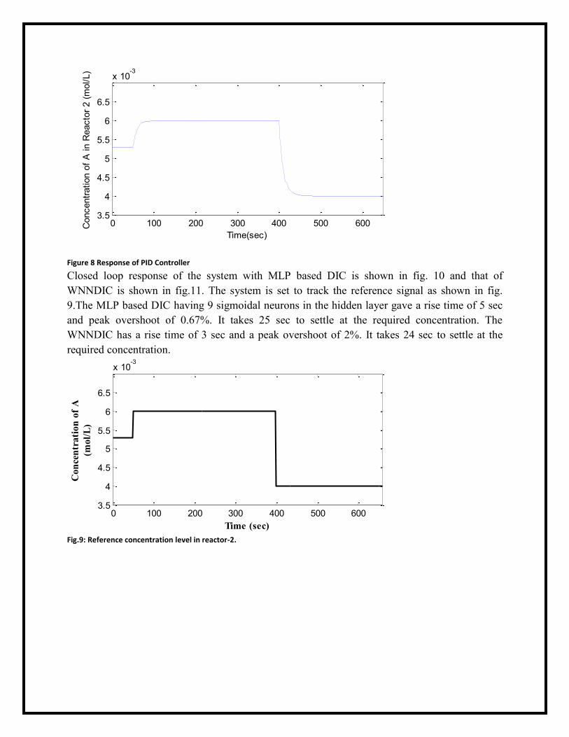
Figure 8 Response of PID Controller
Closed loop response of the system with MLP based DIC is shown in fig. 10 and that of
WNNDIC is shown in fig.11. The system is set to track the reference signal as shown in fig.
9.The MLP based DIC having 9 sigmoidal neurons in the hidden layer gave a rise time of 5 sec
and peak overshoot of 0.67%. It takes 25 sec to settle at the required concentration. The
WNNDIC has a rise time of 3 sec and a peak overshoot of 2%. It takes 24 sec to settle at the
required concentration.
Fig.9: Reference concentration level in reactor-2.
0 100 200 300 400 500 6003.5
4
4.5
5
5.5
6
6.5
x 10-3
Time(sec)
Concentr
ation o
f A
in R
eacto
r 2 (
mol/L)
0 100 200 300 400 500 6003.5
4
4.5
5
5.5
6
6.5
x 10-3
Time (sec)
Co
nce
ntr
ati
on
of
A
(mo
l/L
)

Fig.10: Response of MLP based DIC
Fig.11: Response of WNNDIC
A constant load disturbance in the coolant flow rate of 1 L/min was introduced for a finite
duration to analyze the disturbance handling capability of the MLP based DIC and WNNDIC
strategies. The response of MLP based DIC to disturbance is shown in fig. 13 and that of
WNNDIC is shown in fig. 14. Both the DIC strategies were found to be incapable of handling
constant load disturbances. Post disturbance, the MLP based DIC took 21 sec to return to the set
point while the WNNDIC took 17 sec to return to the set point.
0 100 200 300 400 500 6003.5
4
4.5
5
5.5
6
6.5
x 10-3
Time (sec)
Co
nce
ntr
ati
on
of
A
(mo
l/L
)
0 100 200 300 400 500 6003.5
4
4.5
5
5.5
6
6.5
x 10-3
Time(sec)
Co
nce
ntr
ati
on
of
A
(mo
l/L
)

Fig.12: Disturbance
Fig.23: Response of MLP based DIC to disturbance
Fig.14: Response of WNNDIC to disturbance
0 50 100 150 200 250 300 350 4000
1
2
3
4
5
Time
coo
lan
t F
low
Ra
te
(L/m
in)
0 50 100 150 200 250 300 350 4003.5
4
4.5
5
5.5
6
6.5
x 10-3
Time (sec)
Co
nce
ntr
ati
on
of
A
(mo
l/L
)
0 50 100 150 200 250 300 350 4003.5
4
4.5
5
5.5
6
6.5
x 10-3
Time(sec)
Co
nce
ntr
ati
on
of
A
(mo
l/L
)

The closed loop response of the system with MLP based IMC is shown in fig. 15 and that with
WNNIMC is shown in fig. 16. The system is set to track the same reference signal as shown in
fig. 9. The MLP based IMC having a forward network with 3 inputs, 8 sigmoidal hidden neurons
and 1 output gave a rise time of 14 sec but 0% overshoot. It took 24 sec to settle at the required
set point. The WNNIMC has a same rise time and 0% overshoot but settles in 22 sec.
Fig.3: Response of MLP based IMC
Fig.16: Response of WNNIMC
A constant load disturbance in the coolant flow rate of 1 L/min was introduced for a finite
duration to analyze the disturbance handling capability of the MLP based IMC and WNNIMC
strategies. The response of MLP based IMC to disturbance is shown in fig. 17 and that of
WNNIMC is shown in fig. 18.The MLP based IMC returns back to the set point in 16 sec during
the disturbance period. The WNNIMC returns to the set point in 14 sec. Both the schemes incur
offset peaks at the rising and falling edge of the disturbance graph.
0 100 200 300 400 500 6003.5
4
4.5
5
5.5
6
6.5
x 10-3
Time(sec)
Co
nce
ntr
ati
on
of
A
(mo
l/L
)
0 100 200 300 400 500 6003.5
4
4.5
5
5.5
6
6.5
x 10-3
Time(sec)
Co
nce
ntr
ati
on
of
A
(mo
l/L
)

Fig.17: Response of MLP based IMC to disturbance
Fig.18: Response of WNNIMC to disturbance
6 Conclusion
In the present work, WNN based DIC and IMC control strategies were implemented and
analyzed on a cascaded CSTR model and the result was compared to that obtained from PID
tuning. The constant load disturbance handling capability of these control strategies were also
investigated. PID controller had the highest rise time The WNN based DIC and IMC had reduced
network size and displayed improved robustness as compared to conventional MLP based DIC
and IMC. WNNDIC showed considerably reduced rise time and settling time than MLP based
DIC. IMC strategy was implemented to overcome the inherent inability of the DIC control
strategy to handle load disturbances effectively. Both WNNIMC and MLP based IMC returned
0% peak overshoot and lessened rise time and settling time than their DIC counterparts. Also,
IMC strategy displayed enhanced constant load disturbance handling capability with just two
offset peaks of very short duration; one each at the rising and falling edge of the constant
disturbance. The time duration of the offset peaks were lesser in the case of WNNIMC than MLP
0 50 100 150 200 250 300 350 4003.5
4
4.5
5
5.5
6
6.5
x 10-3
Time(sec)
Co
nce
ntr
ati
on
of
A
(mo
l/L
)
0 50 100 150 200 250 300 350 4003.5
4
4.5
5
5.5
6
6.5
x 10-3
Time(sec)
Co
nce
ntr
ati
on
of
A
(mo
l/L
)
based IMC for same constant disturbance over same duration. The WNNDIC and WNNIMC
were found to be more robust and faster than conventional MLP with considerable reduction in
network sizes.
7 References
[1] Q. Zhang and A. Benveniste. ‘Wavelet networks’, IEEE Transactions on neural networks,
volume 3, pages 889–898, 1992.
[2] Licheng Jiao, ‘Multiwavelet Neural Network And Its Approximation Properties’, IEEE
Transactions on neural networks, VOL. 12, NO. 5, 1060 – 1066 (2001).
[3] Cheng-Jian Lin, ‘Wavelet Neural Networks with a Hybrid Learning Approach’, Journal Of
Information Science And Engineering 22, 1367-1387 (2006).
[4] D.B.Anuradha, G.Prabhaker Reddy, J.S.N.Murthy ‘Direct Inverse Neural Network Control of A
Continuous Stirred Tank Reactor (CSTR)’ Proceedings of the International MultiConference of
Engineers and Computer Scientists 2009 Vol II IMECS 2009, March 18 - 20, 2009, Hong
Kong.
[5] Tarun Varshney, Ruchi Varshney, Satya Sheel ‘ANN Based IMC Scheme for CSTR’
International Conference on Advances in Computing, Communication and Control, ICAC3
2009, Pages 543-546.
[6] Yonghong Tan, Xuanju Dang, Feng Liang, Chun-Yi Su ‘Dynamic Wavelet Neural Network
for Nonlinear Dynamic System Identification’, Proceedings of IEEE International Conference
on Control Applications Anchorage, Alaska, USA September 25-27, 2000, Pages 214-216.
[7] Ehsan Hossaini-asl, Mehdi Shahbazian ‘Nonlinear dynamic system control using wavelet
neural network based on sampling theory’, IEEE International Conference on Systems, Man,
and Cybernetics San Antonio, TX, USA – October 11-14, 2009, Pages 4502-4507.
[8] Hui Li, Chen Guo, Hongzhang Jin ‘Design of Adaptive Inverse Mode Wavelet Neural
Network Controller of Fin Stabilizer’, IEEE International Conference on Neural Networks
and Brain, 2005, Volume 3, Pages 1745-1748.
[9] Hensen, M.A. and Seborg, D.E., ‘Nonlinear Process Control’, Prentice Hall, 1997.