EC 823: Applied Econometrics - fm · PDF fileDynamic Panel Data estimators Christopher F Baum...

Dynamic Panel Data estimators

Christopher F Baum

EC 823: Applied Econometrics

Boston College, Spring 2013

Christopher F Baum (BC / DIW) Dynamic Panel Data estimators Boston College, Spring 2013 1 / 50

Dynamic panel data estimators

Dynamic panel data estimators

In the context of panel data, we usually must deal with unobservedheterogeneity by applying the within (demeaning) transformation, as inone-way fixed effects models, or by taking first differences if thesecond dimension of the panel is a proper time series.

The ability of first differencing to remove unobserved heterogeneityalso underlies the family of estimators that have been developed fordynamic panel data (DPD) models. These models contain one or morelagged dependent variables, allowing for the modeling of a partialadjustment mechanism.


Dynamic panel data estimators Nickell bias

Nickell bias

A serious difficulty arises with the one-way fixed effects model in thecontext of a dynamic panel data (DPD) model particularly in the “smallT , large N" context. As Nickell (Econometrica, 1981) shows, thisarises because the demeaning process which subtracts theindividual’s mean value of y and each X from the respective variablecreates a correlation between regressor and error.

The mean of the lagged dependent variable contains observations 0through (T − 1) on y , and the mean error—which is being conceptuallysubtracted from each εit—contains contemporaneous values of ε fort = 1 . . .T . The resulting correlation creates a bias in the estimate ofthe coefficient of the lagged dependent variable which is not mitigatedby increasing N, the number of individual units.



The demeaning operation creates a regressor which cannot bedistributed independently of the error term. Nickell demonstrates thatthe inconsistency of ρ̂ as N →∞ is of order 1/T , which may be quitesizable in a “small T " context. If ρ > 0, the bias is invariably negative,so that the persistence of y will be underestimated.

For reasonably large values of T , the limit of (ρ̂− ρ) as N →∞ will beapproximately −(1 + ρ)/(T − 1): a sizable value, even if T = 10. Withρ = 0.5, the bias will be -0.167, or about 1/3 of the true value. Theinclusion of additional regressors does not remove this bias. Indeed, ifthe regressors are correlated with the lagged dependent variable tosome degree, their coefficients may be seriously biased as well.



Note also that this bias is not caused by an autocorrelated errorprocess ε. The bias arises even if the error process is i .i .d . If the errorprocess is autocorrelated, the problem is even more severe given thedifficulty of deriving a consistent estimate of the AR parameters in thatcontext.

The same problem affects the one-way random effects model. The uierror component enters every value of yit by assumption, so that thelagged dependent variable cannot be independent of the compositeerror process.



One solution to this problem involves taking first differences of theoriginal model. Consider a model containing a lagged dependentvariable and a single regressor X :

yit = β1 + ρyi,t−1 + Xitβ2 + ui + εit (1)

The first difference transformation removes both the constant term andthe individual effect:

∆yit = ρ∆yi,t−1 + ∆Xitβ2 + ∆εit (2)

There is still correlation between the differenced lagged dependentvariable and the disturbance process (which is now a first-ordermoving average process, or MA(1)): the former contains yi,t−1 and thelatter contains εi,t−1.



But with the individual fixed effects swept out, a straightforwardinstrumental variables estimator is available. We may constructinstruments for the lagged dependent variable from the second andthird lags of y , either in the form of differences or lagged levels. If ε isi .i .d ., those lags of y will be highly correlated with the laggeddependent variable (and its difference) but uncorrelated with thecomposite error process.

Even if we had reason to believe that ε might be following an AR(1)process, we could still follow this strategy, “backing off” one period andusing the third and fourth lags of y (presuming that the timeseries foreach unit is long enough to do so).

This approach is the Anderson–Hsiao (AH) estimator implemented bythe Stata command xtivreg, fd.


Dynamic panel data estimators The DPD approach

The DPD approach

The DPD (Dynamic Panel Data) approach is usually considered thework of Arellano and Bond (AB) (Rev. Ec. Stud., 1991), but they in factpopularized the work of Holtz-Eakin, Newey and Rosen(Econometrica, 1988). It is based on the notion that the instrumentalvariables approach noted above does not exploit all of the informationavailable in the sample. By doing so in a Generalized Method ofMoments (GMM) context, we may construct more efficient estimates ofthe dynamic panel data model.


Dynamic panel data estimators Arellano–Bond estimator

Arellano and Bond argue that the Anderson–Hsiao estimator, whileconsistent, fails to take all of the potential orthogonality conditions intoaccount. A key aspect of the AB strategy, echoing that of AH, is theassumption that the necessary instruments are ‘internal’: that is,based on lagged values of the instrumented variable(s). Theestimators allow the inclusion of external instruments as well.

Consider the equations

yit = Xitβ1 + Witβ2 + vit

vit = ui + εit (3)

where Xit includes strictly exogenous regressors, Wit arepredetermined regressors (which may include lags of y ) andendogenous regressors, all of which may be correlated with ui , theunobserved individual effect. First-differencing the equation removesthe ui and its associated omitted-variable bias.



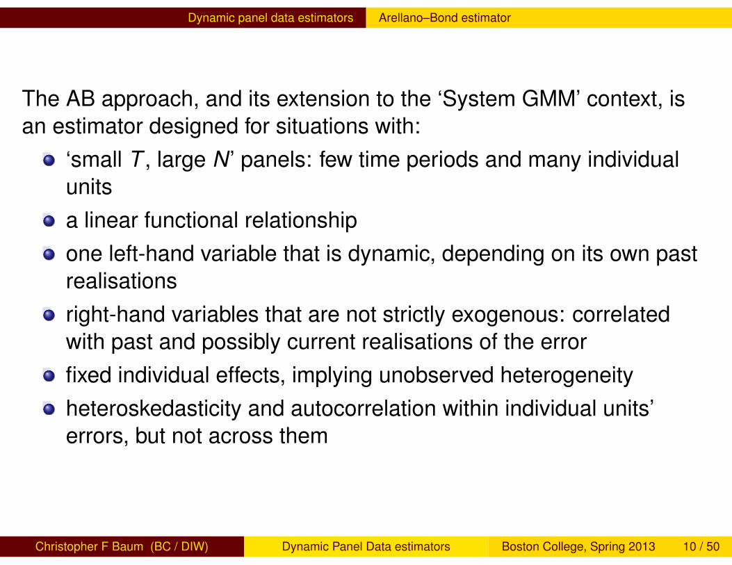
The AB approach, and its extension to the ‘System GMM’ context, isan estimator designed for situations with:

‘small T , large N ’ panels: few time periods and many individualunitsa linear functional relationshipone left-hand variable that is dynamic, depending on its own pastrealisationsright-hand variables that are not strictly exogenous: correlatedwith past and possibly current realisations of the errorfixed individual effects, implying unobserved heterogeneityheteroskedasticity and autocorrelation within individual units’errors, but not across them



The Arellano–Bond estimator sets up a generalized method ofmoments (GMM) problem in which the model is specified as a systemof equations, one per time period, where the instruments applicable toeach equation differ (for instance, in later time periods, additionallagged values of the instruments are available).

This estimator is available in Stata as xtabond. A more generalversion, allowing for autocorrelated errors, is available as xtdpd. Anexcellent alternative to Stata’s built-in commands is David Roodman’sxtabond2, available from SSC (findit xtabond2). It is very welldocumented in his paper, included in your materials. The xtabond2routine provides several additional features—such as the orthogonaldeviations transformation discussed below—not available in officialStata’s commands.


Dynamic panel data estimators Constructing the instrument matrix

Constructing the instrument matrix

In standard 2SLS, including the Anderson–Hsiao approach, thetwice-lagged level appears in the instrument matrix as

Zi =

.

yi,1...

yi,T−2

where the first row corresponds to t = 2, given that the firstobservation is lost in applying the FD transformation. The missingvalue in the instrument for t = 2 causes that observation for eachpanel unit to be removed from the estimation.



If we also included the thrice-lagged level yt−3 as a second instrumentin the Anderson–Hsiao approach, we would lose another observationper panel:

Zi =

. .

yi,1 .yi,2 yi,1

......

yi,T−2 yi,T−3

so that the first observation available for the regression is that datedt = 4.



To avoid this loss of degrees of freedom, Holtz-Eakin et al. construct aset of instruments from the second lag of y , one instrument pertainingto each time period:

Zi =

0 0 . . . 0

yi,1 0 . . . 00 yi,2 . . . 0...

.... . .

...0 0 . . . yi,T−2

The inclusion of zeros in place of missing values prevents the loss ofadditional degrees of freedom, in that all observations dated t = 2 andlater can now be included in the regression. Although the inclusion ofzeros might seem arbitrary, the columns of the resulting instrumentmatrix will be orthogonal to the transformed errors. The resultingmoment conditions correspond to an expectation we believe shouldhold: E(yi,t−2ε

∗it ) = 0, where ε∗ refers to the FD-transformed errors.



It would also be valid to ‘collapse’ the columns of this Z matrix into asingle column, which embodies the same expectation, but conveysless information as it will only produce a single moment condition. Inthis context, the collapsed instrument set will be the same implied bystandard IV, with a zero replacing the missing value in the first usableobservation:

Zi =

0

yi,1...

yi,T−2

This is specified in Roodman’s xtabond2 software by giving thecollapse option.



Given this solution to the tradeoff between lag length and samplelength, we can now adopt Holtz-Eakin et al.’s suggestion and includeall available lags of the untransformed variables as instruments. Forendogenous variables, lags 2 and higher are available. Forpredetermined variables that are not strictly exogenous, lag 1 is alsovalid, as its value is only correlated with errors dated t − 2 or earlier.

Using all available instruments gives rise to an instrument matrix suchas

Zi =

0 0 0 0 0 0 . . .

yi,1 0 0 0 0 0 . . .0 yi,2 yi,1 0 0 0 . . .0 0 0 yi,3 yi,2 yi,1 . . ....

......

......

.... . .



In this setup, we have different numbers of instruments available foreach time period: one for t = 2, two for t = 3, and so on. As we moveto the later time periods in each panel’s timeseries, additionalorthogonality conditions become available, and taking these additionalconditions into account improves the efficiency of the AB estimator.

One disadvantage of this strategy should be apparent. The number ofinstruments produced will be quadratic in T , the length of thetimeseries available. If T < 10, that may be a manageable number, butfor a longer timeseries, it may be necessary to restrict the number ofpast lags used. Both the official Stata commands and Roodman’sxtabond2 allow the specification of the particular lags to be includedin estimation, rather than relying on the default strategy.


Dynamic panel data estimators The System GMM estimator

The System GMM estimator

A potential weakness in the Arellano–Bond DPD estimator wasrevealed in later work by Arellano and Bover (1995) and Blundell andBond (1998). The lagged levels are often rather poor instruments forfirst differenced variables, especially if the variables are close to arandom walk. Their modification of the estimator includes lagged levelsas well as lagged differences.

The original estimator is often entitled difference GMM, while theexpanded estimator is commonly termed System GMM. The cost ofthe System GMM estimator involves a set of additional restrictions onthe initial conditions of the process generating y . This estimator isavailable in Stata as xtdpdsys.


Dynamic panel data estimators Diagnostic tests

Diagnostic tests

As the DPD estimators are instrumental variables methods, it isparticularly important to evaluate the Sargan–Hansen test resultswhen they are applied. Roodman’s xtabond2 provides C tests (asdiscussed in re ivreg2) for groups of instruments. In his routine,instruments can be either “GMM-style" or “IV-style". The former areconstructed per the Arellano–Bond logic, making use of multiple lags;the latter are included as is in the instrument matrix. For the systemGMM estimator (the default in xtabond2) instruments may bespecified as applying to the differenced equations, the level equationsor both.


Dynamic panel data estimators Diagnostic tests

Another important diagnostic in DPD estimation is the AR test forautocorrelation of the residuals. By construction, the residuals of thedifferenced equation should possess serial correlation, but if theassumption of serial independence in the original errors is warranted,the differenced residuals should not exhibit significant AR(2) behavior.These statistics are produced in the xtabond and xtabond2 output.If a significant AR(2) statistic is encountered, the second lags ofendogenous variables will not be appropriate instruments for theircurrent values.

A useful feature of xtabond2 is the ability to specify, for GMM-styleinstruments, the limits on how many lags are to be included. If T isfairly large (more than 7–8) an unrestricted set of lags will introduce ahuge number of instruments, with a possible loss of efficiency. Byusing the lag limits options, you may specify, for instance, that onlylags 2–5 are to be used in constructing the GMM instruments.


Dynamic panel data estimators An empirical exercise

An empirical exercise

To illustrate the performance of the several estimators, we make use ofthe original AB dataset, available within Stata with webuse abdata.This is an unbalanced panel of annual data from 140 UK firms for1976–1984. In their original paper, they modeled firms’ employment nusing a partial adjustment model to reflect the costs of hiring and firing,with two lags of employment.

Other variables included were the current and lagged wage level w, thecurrent, once- and twice-lagged capital stock (k) and the current,once- and twice-lagged output in the firm’s sector (ys). All variablesare expressed as logarithms. A set of time dummies is also included tocapture business cycle effects.



If we were to estimate this model ignoring its dynamic panel nature, wecould merely apply regress with panel-clustered standard errors:

regress n nL1 nL2 w wL1 k kL1 kL2 ys ysL1 ysL2 yr*, cluster(id)

One obvious difficulty with this approach is the likely importance offirm-level unobserved heterogeneity. We have accounted for potentialcorrelation between firms’ errors over time with the cluster-robust VCE,but this does not address the potential impact of unobservedheterogeneity on the conditional mean.

We can apply the within transformation to take account of this aspectof the data:

xtreg n nL1 nL2 w wL1 k kL1 kL2 ys ysL1 ysL2 yr*, fe cluster(id)



The fixed effects estimates will suffer from Nickell bias, which may besevere given the short timeseries available.

OLS FEnL1 1.045∗∗∗ (20.17) 0.733∗∗∗ (12.28)nL2 -0.0765 (-1.57) -0.139 (-1.78)w -0.524∗∗ (-3.01) -0.560∗∗∗ (-3.51)k 0.343∗∗∗ (7.06) 0.388∗∗∗ (6.82)ys 0.433∗ (2.42) 0.469∗∗ (2.74)N 751 751t statistics in parentheses∗ p < 0.05, ∗∗ p < 0.01, ∗∗∗ p < 0.001



In the original OLS regression, the lagged dependent variable waspositively correlated with the error, biasing its coefficient upward. In thefixed effects regression, its coefficient is biased downward due to thenegative sign on νt−1 in the transformed error. The OLS estimate ofthe first lag of n is 1.045; the fixed effects estimate is 0.733.

Given the opposite directions of bias present in these estimates,consistent estimates should lie between these values, which may be auseful check. As the coefficient on the second lag of n cannot bedistinguished from zero, the first lag coefficient should be below unityfor dynamic stability.



To deal with these two aspects of the estimation problem, we mightuse the Anderson–Hsiao estimator to the first-differenced equation,instrumenting the lagged dependent variable with the twice-laggedlevel:

ivregress 2sls D.n (D.nL1 = nL2) D.(nL2 w wL1 k kL1 kL2 ///ys ysL1 ysL2 yr1979 yr1980 yr1981 yr1982 yr1983 )



A-HD.nL1 2.308 (1.17)D.nL2 -0.224 (-1.25)D.w -0.810∗∗ (-3.10)D.k 0.253 (1.75)D.ys 0.991∗ (2.14)N 611t statistics in parentheses∗ p < 0.05, ∗∗ p < 0.01, ∗∗∗ p < 0.001

Although these results should be consistent, they are quitedisappointing. The coefficient on lagged n is outside the bounds of itsOLS and FE counterparts, and much larger than unity, a valueconsistent with dynamic stability. It is also very imprecisely estimated.



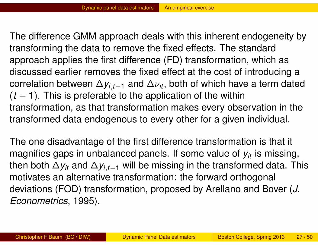
The difference GMM approach deals with this inherent endogeneity bytransforming the data to remove the fixed effects. The standardapproach applies the first difference (FD) transformation, which asdiscussed earlier removes the fixed effect at the cost of introducing acorrelation between ∆yi,t−1 and ∆νit , both of which have a term dated(t − 1). This is preferable to the application of the withintransformation, as that transformation makes every observation in thetransformed data endogenous to every other for a given individual.

The one disadvantage of the first difference transformation is that itmagnifies gaps in unbalanced panels. If some value of yit is missing,then both ∆yit and ∆yi,t−1 will be missing in the transformed data. Thismotivates an alternative transformation: the forward orthogonaldeviations (FOD) transformation, proposed by Arellano and Bover (J.Econometrics, 1995).



In contrast to the within transformation, which subtracts the average ofall observations’ values from the current value, and the FDtransformation, that subtracts the previous value from the currentvalue, the FOD transformation subtracts the average of all availablefuture observations from the current value. While the FDtransformation drops the first observation on each individual in thepanel, the FOD transformation drops the last observation for eachindividual. It is computable for all periods except the last period, evenin the presence of gaps in the panel.

The FOD transformation is not available in any of official Stata’s DPDcommands, but it is available in David Roodman’s xtabond2implementation of the DPD estimator, available from SSC.



To illustrate the use of the AB estimator, we may reestimate the modelwith xtabond2, assuming that the only endogeneity present is thatinvolving the lagged dependent variable.

xtabond2 n L(1/2).n L(0/1).w L(0/2).(k ys) yr*, gmm(L.n) ///iv(L(0/1).w L(0/2).(k ys) yr*) nolevel robust small

Note that in xtabond2 syntax, every right-hand variable generallyappears twice in the command, as instruments must be explicitlyspecified when they are instrumenting themselves. In this example, allexplanatory variables except the lagged dependent variable are takenas “IV-style” instruments, entering the Z matrix as a single column. Thelagged dependent variable is specified as a “GMM-style” instrument,where all available lags will be used as separate instruments. Thenoleveleq option is needed to specify the AB estimator.



A-BL.n 0.686∗∗∗ (4.67)L2.n -0.0854 (-1.50)w -0.608∗∗ (-3.36)k 0.357∗∗∗ (5.95)ys 0.609∗∗∗ (3.47)N 611t statistics in parentheses∗ p < 0.05, ∗∗ p < 0.01, ∗∗∗ p < 0.001

In these results, 41 instruments have been created, with 17corresponding to the “IV-style” regressors and the rest computed fromlagged values of n. Note that the coefficient on the lagged dependentvariable now lies within the range for dynamic stability. In contrast tothat produced by the Anderson–Hsiao estimator, the coefficient is quiteprecisely estimated.



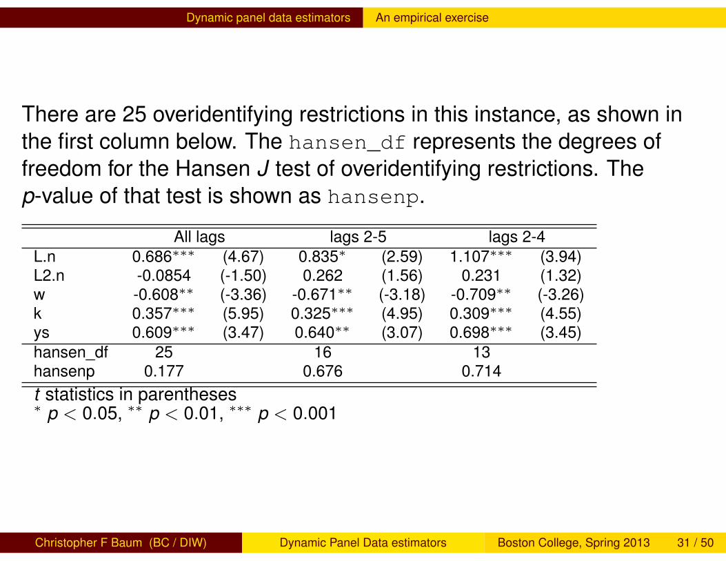
There are 25 overidentifying restrictions in this instance, as shown inthe first column below. The hansen_df represents the degrees offreedom for the Hansen J test of overidentifying restrictions. Thep-value of that test is shown as hansenp.

All lags lags 2-5 lags 2-4L.n 0.686∗∗∗ (4.67) 0.835∗ (2.59) 1.107∗∗∗ (3.94)L2.n -0.0854 (-1.50) 0.262 (1.56) 0.231 (1.32)w -0.608∗∗ (-3.36) -0.671∗∗ (-3.18) -0.709∗∗ (-3.26)k 0.357∗∗∗ (5.95) 0.325∗∗∗ (4.95) 0.309∗∗∗ (4.55)ys 0.609∗∗∗ (3.47) 0.640∗∗ (3.07) 0.698∗∗∗ (3.45)hansen_df 25 16 13hansenp 0.177 0.676 0.714t statistics in parentheses∗ p < 0.05, ∗∗ p < 0.01, ∗∗∗ p < 0.001



In this table, we can examine the sensitivity of the results to the choiceof “GMM-style” lag specification. In the first column, all available lagsof the level of n are used. In the second column, the lag(2 5) optionis used to restrict the maximum lag to 5 periods, while in the thirdcolumn, the maximum lag is set to 4 periods. Fewer instruments areused in those instances, as shown by the smaller values of sar_df.

The p-value of Hansen’s J is also considerably larger for therestricted-lag cases. On the other hand, the estimate of the laggeddependent variable’s coefficient appears to be quite sensitive to thechoice of lag length.



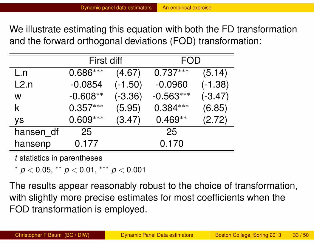
We illustrate estimating this equation with both the FD transformationand the forward orthogonal deviations (FOD) transformation:

First diff FODL.n 0.686∗∗∗ (4.67) 0.737∗∗∗ (5.14)L2.n -0.0854 (-1.50) -0.0960 (-1.38)w -0.608∗∗ (-3.36) -0.563∗∗∗ (-3.47)k 0.357∗∗∗ (5.95) 0.384∗∗∗ (6.85)ys 0.609∗∗∗ (3.47) 0.469∗∗ (2.72)hansen_df 25 25hansenp 0.177 0.170t statistics in parentheses∗ p < 0.05, ∗∗ p < 0.01, ∗∗∗ p < 0.001

The results appear reasonably robust to the choice of transformation,with slightly more precise estimates for most coefficients when theFOD transformation is employed.



We might reasonably consider, as did Blundell and Bond (J.Econometrics, 1998), that wages and the capital stock should not betaken as strictly exogenous in this context, as we have in the abovemodels.

Reestimate the equation producing “GMM-style” instruments for allthree variables, with both one-step and two-step VCE:

xtabond2 n L(1/2).n L(0/1).w L(0/2).(k ys) yr*, gmm(L.(n w k)) ///iv(L(0/2).ys yr*) nolevel robust small



One-step Two-stepL.n 0.818∗∗∗ (9.51) 0.824∗∗∗ (8.51)L2.n -0.112∗ (-2.23) -0.101 (-1.90)w -0.682∗∗∗ (-4.78) -0.711∗∗∗ (-4.67)k 0.353∗∗ (2.89) 0.377∗∗ (2.79)ys 0.651∗∗∗ (3.43) 0.662∗∗∗ (3.89)hansen_df 74 74hansenp 0.487 0.487t statistics in parentheses∗ p < 0.05, ∗∗ p < 0.01, ∗∗∗ p < 0.001

The results from both one-step and two-step estimation appearreasonable. Interestingly, only the coefficient on ys appears to be moreprecisely estimated by the two-step VCE. With no restrictions on theinstrument set, 74 overidentifying restrictions are defined, with 90instruments in total.


Dynamic panel data estimators Illustration of system GMM

To illustrate system GMM, we follow Blundell and Bond, who used thesame abdata dataset on a somewhat simpler model, dropping thesecond lags and removing sectoral demand. We consider wages andcapital as potentially endogenous, with GMM-style instruments.

Estimate the one-step BB model.

xtabond2 n L.n L(0/1).(w k) yr*, gmm(L.(n w k)) iv(yr*, equation(level)) ///robust small

We indicate here with the equation(level) suboption that the yeardummies are only to be considered instruments in the level equation.As the default for xtabond2 is the BB estimator, we omit thenoleveleq option that has called for the AB estimator in earlierexamples.


Dynamic panel data estimators Illustration of system GMM

nL.n 0.936∗∗∗ (35.21)w -0.631∗∗∗ (-5.29)k 0.484∗∗∗ (8.89)hansen_df 100hansenp 0.218t statistics in parentheses∗ p < 0.05, ∗∗ p < 0.01, ∗∗∗ p < 0.001

We find that the α coefficient is much higher than in the AB estimates,although it may be distinguished from unity. 113 instruments arecreated, with 100 degrees of freedom in the test of overidentifyingrestrictions.


Dynamic panel data estimators A second empirical exercise

A second empirical exercise

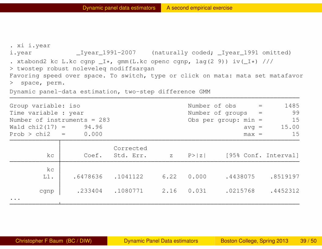
We also illustrate DPD estimation using the Penn World Tablecross-country panel. We specify a model for kc (the consumptionshare of real GDP per capita) depending on its own lag, cgnp, and aset of time fixed effects, which we compute with the xi command, asxtabond2 does not support factor variables.

We first estimate the two-step ‘difference GMM’ form of the model with(cluster-)robust VCE, using data for 1991–2007. We could usetestparm _I* after estimation to evaluate the joint significance oftime effects (listing of which has been suppressed).



. xi i.yeari.year _Iyear_1991-2007 (naturally coded; _Iyear_1991 omitted)

. xtabond2 kc L.kc cgnp _I*, gmm(L.kc openc cgnp, lag(2 9)) iv(_I*) ///> twostep robust noleveleq nodiffsarganFavoring speed over space. To switch, type or click on mata: mata set matafavor> space, perm.

Dynamic panel-data estimation, two-step difference GMM

Group variable: iso Number of obs = 1485Time variable : year Number of groups = 99Number of instruments = 283 Obs per group: min = 15Wald chi2(17) = 94.96 avg = 15.00Prob > chi2 = 0.000 max = 15

Correctedkc Coef. Std. Err. z P>|z| [95% Conf. Interval]

kcL1. .6478636 .1041122 6.22 0.000 .4438075 .8519197

cgnp .233404 .1080771 2.16 0.031 .0215768 .4452312...



(continued)

Instruments for first differences equationStandardD.(_Iyear_1992 _Iyear_1993 _Iyear_1994 _Iyear_1995 _Iyear_1996 _Iyear_1997_Iyear_1998 _Iyear_1999 _Iyear_2000 _Iyear_2001 _Iyear_2002 _Iyear_2003_Iyear_2004 _Iyear_2005 _Iyear_2006 _Iyear_2007)

GMM-type (missing=0, separate instruments for each period unless collapsed)L(2/9).(L.kc openc cgnp)

Arellano-Bond test for AR(1) in first differences: z = -2.94 Pr > z = 0.003Arellano-Bond test for AR(2) in first differences: z = 0.23 Pr > z = 0.815

Sargan test of overid. restrictions: chi2(266) = 465.53 Prob > chi2 = 0.000(Not robust, but not weakened by many instruments.)

Hansen test of overid. restrictions: chi2(266) = 87.81 Prob > chi2 = 1.000(Robust, but can be weakened by many instruments.)



Given the relatively large number of time periods available, I havespecified that the GMM instruments only be constructed for lags 2–9 tokeep the number of instruments manageable. I am treating openc asa GMM-style instrument. The autoregressive coefficient is 0.648, andthe cgnp coefficient is positive and significant. Although not shown,the test for joint significance of the time effects has p-value 0.0270.

We could also fit this model with the ‘system GMM’ estimator, whichwill be able to utilize one more observation per country in the levelequation, and estimate a constant term in the relationship. I amtreating lagged openc as a IV-style instrument in this specification.



. xtabond2 kc L.kc cgnp _I*, gmm(L.kc cgnp, lag(2 8)) iv(_I* L.openc) ///> twostep robust nodiffsargan

Dynamic panel-data estimation, two-step system GMM



kcL1. .9452696 .0191167 49.45 0.000 .9078014 .9827377

cgnp .097109 .0436338 2.23 0.026 .0115882 .1826297...

_cons -6.091674 3.45096 -1.77 0.078 -12.85543 .672083



(continued)

Instruments for first differences equationStandardD.(_Iyear_1992 _Iyear_1993 _Iyear_1994 _Iyear_1995 _Iyear_1996 _Iyear_1997_Iyear_1998 _Iyear_1999 _Iyear_2000 _Iyear_2001 _Iyear_2002 _Iyear_2003_Iyear_2004 _Iyear_2005 _Iyear_2006 _Iyear_2007 L.openc)

GMM-type (missing=0, separate instruments for each period unless collapsed)L(2/8).(L.kc cgnp)

Instruments for levels equationStandard_cons_Iyear_1992 _Iyear_1993 _Iyear_1994 _Iyear_1995 _Iyear_1996 _Iyear_1997_Iyear_1998 _Iyear_1999 _Iyear_2000 _Iyear_2001 _Iyear_2002 _Iyear_2003_Iyear_2004 _Iyear_2005 _Iyear_2006 _Iyear_2007 L.openc

GMM-type (missing=0, separate instruments for each period unless collapsed)DL.(L.kc cgnp)






Note that the autoregressive coefficient is much larger: 0.945 in thiscontext. The cgnp coefficient is again positive and significant, but hasa much smaller magnitude when the system GMM estimator is used.

We can also estimate the model using the forward orthogonaldeviations (FOD) transformation of Arellano and Bover, as described inRoodman’s paper. The first-difference transformation applied in DPDestimators has the unfortunate feature of magnifying any gaps in thedata, as one period of missing data is replaced with two missingdifferences. FOD transforms each observation by subtracting theaverage of all future observations, which will be defined (regardless ofgaps) for all but the last observation in each panel. To illustrate:



. xtabond2 kc L.kc cgnp _I*, gmm(L.kc cgnp, lag(2 8)) iv(_I* L.openc) ///> twostep robust nodiffsargan orthog

Dynamic panel-data estimation, two-step system GMM



kcL1. .9550247 .0142928 66.82 0.000 .9270114 .983038

cgnp .0723786 .0339312 2.13 0.033 .0058746 .1388825...

_cons -4.329945 2.947738 -1.47 0.142 -10.10741 1.447515



(continued)

Instruments for orthogonal deviations equationStandardFOD.(_Iyear_1992 _Iyear_1993 _Iyear_1994 _Iyear_1995 _Iyear_1996_Iyear_1997 _Iyear_1998 _Iyear_1999 _Iyear_2000 _Iyear_2001 _Iyear_2002_Iyear_2003 _Iyear_2004 _Iyear_2005 _Iyear_2006 _Iyear_2007 L.openc)

GMM-type (missing=0, separate instruments for each period unless collapsed)L(2/8).(L.kc cgnp)

Instruments for levels equationStandard_cons_Iyear_1992 _Iyear_1993 _Iyear_1994 _Iyear_1995 _Iyear_1996 _Iyear_1997_Iyear_1998 _Iyear_1999 _Iyear_2000 _Iyear_2001 _Iyear_2002 _Iyear_2003_Iyear_2004 _Iyear_2005 _Iyear_2006 _Iyear_2007 L.openc

GMM-type (missing=0, separate instruments for each period unless collapsed)DL.(L.kc cgnp)






Using the FOD transformation, the autoregressive coefficient is a bitlarger, and the cgnp coefficient a bit smaller, although its significanceis retained.

After any DPD estimation command, we may save predicted values orresiduals and graph them against the actual values:



. predict double kchat if inlist(country, "Italy", "Spain", "Greece", "Portugal> ")(option xb assumed; fitted values)(1619 missing values generated)

. label var kc "Consumption / Real GDP per capita"

. xtline kc kchat if !mi(kchat), scheme(s2mono)



5560

6570

5560

6570

1990 1995 2000 2005 1990 1995 2000 2005

ESP GRC

ITA PRT

Consumption / Real GDP per capita Fitted Values

year

Graphs by ISO country code



Although the DPD estimators are linear estimators, they are highlysensitive to the particular specification of the model and itsinstruments: more so in my experience than any otherregression-based estimation approach.

There is no substitute for experimentation with the various parametersof the specification to ensure that your results are reasonably robust tovariations in the instrument set and lags used. A very useful referencefor DPD modeling is David Roodman’s paper “How to do xtabond2”paper, freely downloadable from the Stata Journal via IDEAS orEconPapers.


EC 823: Applied Econometrics - fm · PDF fileDynamic Panel Data estimators Christopher F Baum...

Documents

Transcript of EC 823: Applied Econometrics - fm · PDF fileDynamic Panel Data estimators Christopher F Baum...