
eBook.comp Electronics
236
Computational Electronics Dragica Vasileska and Stephen M. Goodnick Department of Electrical Engineering Arizona State University 1
-
Upload
vivek-gupta -
Category
Documents
-
view
719 -
download
0
Transcript of eBook.comp Electronics

5/13/2018 eBook.comp Electronics - slidepdf.com
http://slidepdf.com/reader/full/ebookcomp-electronics 1/236
Computational Electronics
Dragica Vasileska and Stephen M. Goodnick
Department of Electrical Engineering
Arizona State University
1

5/13/2018 eBook.comp Electronics - slidepdf.com
http://slidepdf.com/reader/full/ebookcomp-electronics 2/236
1. Introduction to Computational Electronics .............................................................................42. Semiconductor Fundamentals ...............................................................................................11
2.1. Semiconductor Bandstructure ...........................................................................................112.2. Simplified Band Structure Models ....................................................................................142.3. Carrier Dynamics ..............................................................................................................16
2.4. Effective Mass in Semiconductors ....................................................................................172.5. Semiclassical Transport Theory ........................................................................................212.5.1. Approximations made for the distribution function .....................................................22
2.6. Boltzmann transport equation ...........................................................................................262.7. Scattering Processes ..........................................................................................................292.8. Relaxation-time approximation ........................................................................................312.9. Solving the BTE in the Relaxation Time Approximation ................................................33
3. The Drift-Diffusion Equations and Their Numerical Solution .............................................403.1. Drift-diffusion model ........................................................................................................40
3.1.1. Physical Limitations on Numerical Drift-Diffusion Schemes .....................................423.1.2. Steady State Solution of Bipolar Semiconductor Equations ........................................45
3.1.3. Normalization and Scaling ...........................................................................................473.1.4. Gummel's Iteration Method .........................................................................................483.1.5. Newton's Method .........................................................................................................533.1.6. Generation and Recombination ....................................................................................553.1.7. Time-dependent simulation .........................................................................................563.1.8. Scharfetter-Gummel approximation ............................................................................613.1.9. Extension of the Validity of the Drift-Diffusion Model ..............................................63
4. Hydrodynamic Model ..........................................................................................................714.1. Extensions of the Drift-Diffusion model .......................................................................... 724.2. Stratton’s Approach ..........................................................................................................744.3. Balance Equations Model ................................................................................................. 75
4.3.1. Displaced Maxwellian Approximation ........................................................................814.3.2. Momentum and Energy Relaxation Rates ...................................................................834.3.3. Simplifications That Lead to the Drift-Diffusion Model .............................................85
4.4. Numerical Solution Schemes for the Hydrodynamic Equations ......................................875. Use of Commercially Available Device Simulators .............................................................97
5.1. The need for semiconductor device modeling ..................................................................975.1.1. Importance of semiconductor device simulators .........................................................975.1.2. Key elements of physical device simulation ................................................................985.1.3. Historical Development of the Physical Device Modeling ..........................................99
5.2. Introduction to the Silvaco Atlas Simulation tool ...........................................................1015.2.1. The ATLAS syntax .................................................................................................... 102
5.2.2. Choice of the numerical method ................................................................................1045.2.3. Solutions obtained ......................................................................................................1075.2.4. Advanced Solution Techniques ................................................................................. 1085.2.5. Run-time output, log files, solution files and the extract statement ...........................111
5.3. Examples of Silvaco ATLAS Simulations ..................................................................... 1135.3.1. pn-diode ..................................................................................................................... 1135.3.2. MOSFET Devices ......................................................................................................1195.3.3. Simulation of BJT ...................................................................................................... 129
2

5/13/2018 eBook.comp Electronics - slidepdf.com
http://slidepdf.com/reader/full/ebookcomp-electronics 3/236
5.3.4. Simulation of SOI devices .........................................................................................1405.3.5. Gate Tunneling Models ..............................................................................................1465.3.6. RF simulation of a MESFET (Smiths charts) ............................................................ 150
i. Particle Based Device Simulation Methods .........................................................................1575.4. Free Flight Generation ....................................................................................................158
5.5. Final State After Scattering .............................................................................................1615.6. Ensemble Monte Carlo Simulation .................................................................................1665.7. Multi-Carrier Effects .......................................................................................................170
5.7.1. Pauli exclusion principle ............................................................................................1715.7.2. Carrier-carrier interactions ........................................................................................1715.7.3. Band to Band Impact Ionization ................................................................................ 1745.7.4. Full-Band Particle Based Simulation .........................................................................1755.7.5. Device Simulation Using Particles ............................................................................ 177
5.8. Device Simulation Using Particles ................................................................................. 1785.8.1. Monte Carlo Device Simulation ................................................................................ 1795.8.2. Direct Treatment of Inter-Particle Interaction ........................................................... 193
Appendix A: Numerical Solution of Algebraic Equations .................................................... 204A.1 Direct Methods ...............................................................................................................2055.8.1. A.1.1 Gauss Elimination Method ...............................................................................2055.8.2. A.1.2 The LU Decomposition Method ...................................................................... 2065.8.3. A.1.3 LU Decomposition in 1D .................................................................................207A.2 Iterative Methods .......................................................................................................... 2085.8.4. A.2.1 The Gauss Seidel Method ................................................................................ 2095.8.5. A.2.2 The Successive Over-Relaxation (SOR) Method ............................................ 2105.8.6. A.2.3 Other Iterative Methods ................................................................................... 211
Appendix B: Mobility Modeling and Characterization ......................................................... 218B.1 Experimental Mobilities .................................................................................................219
5.8.1. a) Hall mobility .......................................................................................................... 2195.8.2. b2) MOSFET Mobilities ............................................................................................221B.2 Mobility Modeling ......................................................................................................... 223
3

5/13/2018 eBook.comp Electronics - slidepdf.com
http://slidepdf.com/reader/full/ebookcomp-electronics 4/236
1. Introduction to Computational Electronics
As semiconductor feature sizes shrink into the nanometer scale regime, evenconventional device behavior becomes increasingly complicated as new physical phenomena at
short dimensions occur, and limitations in material properties are reached [1]. In addition to the
problems related to the understanding of actual operation of ultra-small devices, the reduced
feature sizes require more complicated and time-consuming manufacturing processes. This fact
signifies that a pure trial-and-error approach to device optimization will become impossible since
it is both too time consuming and too expensive. Since computers are considerably cheaper
resources, simulation is becoming an indispensable tool for the device engineer. Besides
offering the possibility to test hypothetical devices which have not (or could not) yet been
manufactured, simulation offers unique insight into device behavior by allowing the observation
of phenomena that can not be measured on real devices. Computational Electronics [2,3] in this
context refers to the physical simulation of semiconductor devices in terms of charge transport
and the corresponding electrical behavior. It is related to, but usually separate from process
simulation, which deals with various physical processes such as material growth, oxidation,
impurity diffusion, etching, and metal deposition inherent in device fabrication [ 4] leading to
integrated circuits. Device simulation can be thought of as one component of technology for
computer-aided design (TCAD), which provides a basis for device modeling, which deals with
compact behavioral models for devices and sub-circuits relevant for circuit simulation in
commercial packages such as SPICE [5]. The relationship between various simulation design
steps that have to be followed to achieve certain customer need is illustrated in Figure 1.1.
4

5/13/2018 eBook.comp Electronics - slidepdf.com
http://slidepdf.com/reader/full/ebookcomp-electronics 5/236
Customer Need
Process Simulation
Device Simulation
Parameter Extraction
Circuit Level Simulation
yes
Computational
Electronics
no
Figure 1.1 Design sequence to achieve desired customer need.
The goal of Computational Electronics is to provide simulation tools with the necessary
level of sophistication to capture the essential physics while at the same time minimizing the
computational burden so that results may be obtained within a reasonable time frame. Figure 1.2
illustrates the main components of semiconductor device simulation at any level. There are two
main kernels, which must be solved self-consistently with one another, the transport equations
governing charge flow, and the fields driving charge flow. Both are coupled strongly to one
another, and hence must be solved simultaneously. The fields arise from external sources, as
well as the charge and current densities which act as sources for the time varying electric and
magnetic fields obtained from the solution of Maxwell’s equations. Under appropriate
conditions, only the quasi-static electric fields arising from the solution of Poisson’s equation are
necessary.
5

5/13/2018 eBook.comp Electronics - slidepdf.com
http://slidepdf.com/reader/full/ebookcomp-electronics 6/236
Figure 1.2. Schematic description of the device simulation sequence.
The fields, in turn, are driving forces for charge transport as illustrated in Figure 1.3 for
the various levels of approximation within a hierarchical structure ranging from compact
modeling at the top to an exact quantum mechanical description at the bottom. At the very
beginnings of semiconductor technology, the electrical device characteristics could be estimated
using simple analytical models (gradual channel approximation for MOSFETs) relying on the
drift-diffusion (DD) formalism. Various approximations had to be made to obtain closed-form
solutions, but the resulting models captured the basic features of the devices [6]. These
approximations include simplified doping profiles and device geometries. With the ongoing
refinements and improvements in technology, these approximations lost their basis and a more
accurate description was required. This goal could be achieved by solving the DD equations
numerically. Numerical simulation of carrier transport in semiconductor devices dates back to
the famous work of Scharfetter and Gummel [7], who proposed a robust discretization of the DD
equations which is still in use today.
6

5/13/2018 eBook.comp Electronics - slidepdf.com
http://slidepdf.com/reader/full/ebookcomp-electronics 7/236
Model Improvements
Compact models Appropriate for CircuitDesign
Drift-Diffusion
equations
Good for devices down to
0.5 µm, include µ(E)
HydrodynamicEquations
Velocity overshoot effect canbe treated properly
Boltzmann TransportEquation
Monte Carlo/CA methods
Accurate up to the classicallimits
QuantumHydrodynamics
Keep all classicalhydrodynamic features +
quantum corrections
Approximate Easy, fas
Exact Difficult
S e m
i - c l a s s
i c a l a
p p r o a c
h e s
Q u a n
t u m
a p p r o a c
h e s
Quantum-Kinetic Equation(Liouville , Wigner-Boltzmann )
Accurate up to single particledescription
Green's Functions methodIncludes correlations in both
space and time domain
QuantumMonte Carlo/CA methods
Keep all classicalfeatures + quantum corrections
Direct solution of the n-bodySchrödinger equation
Can be solved only for smallnumber of particles
Figure 1.3. Illustration of the hierarchy of transport models.
However, as semiconductor devices were scaled into the submicrometer regime, the
assumptions underlying the DD model lost their validity. Therefore, the transport models have
been continuously refined and extended to more accurately capture transport phenomena
occurring in these devices. The need for refinement and extension is primarily caused by the
ongoing feature size reduction in state-of-the-art technology. As the supply voltages can not be
scaled accordingly without jeopardizing the circuit performance, the electric field inside the
devices has increased. A large electric field which rapidly changes over small length scales gives
rise to non-local and hot-carrier effects which begin to dominate device performance. An
accurate description of these phenomena is required and is becoming a primary concern for
industrial applications.
To overcome some of the limitations of the DD model, extensions have been proposed
which basically add an additional balance equation for the average carrier energy [8].
7

5/13/2018 eBook.comp Electronics - slidepdf.com
http://slidepdf.com/reader/full/ebookcomp-electronics 8/236
Furthermore, an additional driving term is added to the current expression which is proportional
to the gradient of the carrier temperature. However, a vast number of these models exist, and
there is a considerable amount of confusion as to their relation to each other. It is now a common
practice in industry to use standard hydrodynamic models in trying to understand the operation
of as-fabricated devices, by adjusting any number of phenomenological parameters (e.g.
mobility, impact ionization coefficient, etc.). However, such tools do not have predictive
capability for ultra-small structures, for which it is necessary to relax some of the approximations
in the Boltzmann transport equation [9]. Therefore, one needs to move downward to the quantum
transport area in the hierarchical map of transport models shown in Figure 1.3 where, at the very
bottom we have the Green's function approach [10,11,12]. The latter is the most exact, but at the
same time the most difficult of all. In contrast to, for example, the Wigner function approach
(which is Markovian in time), the Green's functions method allows one to consider
simultaneously correlations in space and time, both of which are expected to be important in
nano-scale devices. However, the difficulties in understanding the various terms in the resultant
equations and the enormous computational burden needed for its actual implementation make the
usefulness in understanding quantum effects in actual devices of limited values. For example,
the only successful utilization of the Green's function approach commercially is the NEMO
(Nano-Electronics MOdeling) simulator [13], which is effectively 1D and is primarily applicable
to resonant tunneling diodes.From the discussion above it follows that, contrary to the recent technological advances,
the present state of the art in device simulation is currently lacking in the ability to treat these
new challenges in scaling of device dimensions from conventional down to quantum scale
devices. For silicon devices with active regions below 0.2 microns in diameter, macroscopic
transport descriptions based on drift-diffusion models are clearly inadequate. As already noted,
even standard hydrodynamic models do not usually provide a sufficiently accurate description
since they neglect significant contributions from the tail of the phase space distribution function
in the channel regions [14,15]. Within the requirement of self-consistently solving the coupled
transport-field problem in this emerging domain of device physics, there are several
computational challenges, which limit this ability. One is the necessity to solve both the
transport and the Poisson's equations over the full 3D domain of the device (and beyond if one
includes radiation effects). As a result, highly efficient algorithms targeted to high-end
8

5/13/2018 eBook.comp Electronics - slidepdf.com
http://slidepdf.com/reader/full/ebookcomp-electronics 9/236
computational platforms (most likely in a multi-processor environment) are required to fully
solve even the appropriate field problems. The appropriate level of approximation necessary to
capture the proper non-equilibrium transport physics relevant to a future device model is an even
more challenging problem both computationally and from a fundamental physics framework.
In this book, we give an overview of the basic techniques used in the field of
Computational Electronics related to device simulation. The multiple scale transport in doped
semiconductors is summarized in Figure 1.4 in terms of the transport regimes, relative
importance of the scattering mechanisms and possible applications.
e ph L l −<< ~ e ph L l − e ph L l −>>
L λ <e e L l −< e e L l −>>
Transport Regime Quantum Ballistic Fluid Fluid DiffusiveScattering Rare Rare e-e (Many), e-ph (Few) ManyModel:
Drift-Diffusion
Hydrodynamic
Monte Carlo
Schrodinger/Green’s
Functions
Quantum Hydrodynamic
Wave
Applications Nanowires,Superlattices
BallisticTransistor Current IC’s Current IC’s Older IC’s
Figure 1.4. Relationship between various transport regimes and significant length-scales.
The book is organized as follows. In Chapter 2 we introduce some basic concepts, such as band-
structure, carrier dynamics, effective masses, etc. In Chapter 3 we introduce the drift-diffusion
model via introduction of the Boltzmann Transport Equation (BTE) and the relaxation time
approximation. Discretization schemes for the Poisson and the continuity equations are also
elaborated in this chapter. The balance equations and their corresponding explicit time
discretization schemes are discussed in Chapter 4. Chapter 5 is probably the most useful chapter
to the user. In this chapter, although the emphasis is on the usage of the SILVACO simulation
software, the discussion presented is very general and the points made are applicable to any
device simulation software. Particularly important are the examples given and the hints on how
9

5/13/2018 eBook.comp Electronics - slidepdf.com
http://slidepdf.com/reader/full/ebookcomp-electronics 10/236
to perform more effective simulations. The Ensemble Monte Carlo technique (EMC) for the
solution of the BTE is discussed in Chapter 6, thus completing the main goal of this book to
cover the various methods used in semiclassical device simulation. The Appendix A is included
to introduce the reader in solving linear algebraic equations of the form Ax=b, where A is a
sparse matrix and special solution techniques apply. In Appendix B we discuss mobility
measurement techniques and the mobility modeling as is usually done in arbitrary device
simulator.
10

5/13/2018 eBook.comp Electronics - slidepdf.com
http://slidepdf.com/reader/full/ebookcomp-electronics 11/236
2. Semiconductor Fundamentals
In this Chapter, we provide a brief review of semiconductor physics relevant to the needs
of Computational Electronics. We begin with a brief review of the electronic states in a periodic
potential as seen by electrons in crystalline semiconductor materials, i.e. the semiconductor
bandstructure. We then introduce the important concepts of effective mass and density of states.
We then look at transport in semiconductors through the semi-classical Boltzmann Transport
Equation (BTE), which is the basis for all the transport simulation methods discussed in the
present volume, and look at some simplifying assumptions such as the relaxation time
approximation for its solutions.
2.1.Semiconductor Bandstructure
The basis for discussing transport in semiconductors is the underlying electronic band
structure of the material arising from the solution of the many body Schrödinger equation in the
presence of the periodic potential of the lattice, which is discussed in a host of solid state physics
textbooks. The solution of the one-particle Schrödinger equation in the presence of the periodic
potential of the lattice (and all the other electronics by an effective one-particle potential) are in
the form of Bloch functions
( ) ( ) rk k k rr ⋅= i
nn eu ,,ψ (2.1)
where k is the wavevector, and n labels the band index corresponding to different solutions for a
given wavevector. The cell-periodic function, ( )rk ,nu , has the periodicity of the lattice and
modulates the traveling wave solution associated with the free particle motion of electrons. The
energy eigenvalues, E n(k ), associated with the Bloch eigenfunctions, k ,nψ above, form what is
commonly referred to as the energy bandstructure. The energy, E n(k ), is periodic as a function of
k , with a periodicity corresponding to the reciprocal lattice associated with the real-space lattice.
The energy is therefore uniquely specified within the unit cell of this reciprocal lattice, referred
to as the first Brillouin zone.
In the usual quantum mechanical picture associated with the wave-particle duality of
matter, the electron motion through the crystal is visualized as a localized wave-packet space
composed of a superposition of Bloch states of different wavevectors around an average
11

5/13/2018 eBook.comp Electronics - slidepdf.com
http://slidepdf.com/reader/full/ebookcomp-electronics 12/236
wavevector, k . The expectation value of the particle velocity then corresponds to the group
velocity of this wave-packet, or
( )k vk n E ∇=
1
(2.2)
A brief look at the symmetry properties of the Bloch functions gives some insight into the
nature of the bandstructure in semiconductors. First consider the atomic orbitals of the
individual atoms that constitute the semiconductor crystal. Typical semiconductors have an
average of 4 valence electrons per atom composed of partially filled s- and p-type orbitals that
contribute to bonding, primarily tetrahedral bonds that formed through sp3 hybridization. The
symmetry (or geometric) properties of these atomic orbitals are apparent from consideration of
their angular components
1
3 sin cos
3 sin sin
3cos
x
y
z
s
x p
r
y p
r
z p
r
θ ϕ
θ ϕ
θ
=
= =
= =
= =
(2.3)
Let us denote these states by |S>, |X>, |Y> and |Z>. When individual atoms are brought together,
these orbitals combine or hybridize into sp3 molecular orbitals to form covalent bonds composed
of lower energy, filled ‘bonding’ molecular orbitals, and unfilled ‘anti-bonding’ orbitals. The
separation in energy between the bonding and anti-bonding orbital states can be viewed as the
fundamental origin of the energy ‘gap’ characteristic of all semiconductors. Once all the atoms
coalesce to form a crystal, these molecular orbitals overlap and broaden, leading to the energy
bandstructure with gaps and allowed energy bands. The mostly filled valence bands are formed
primarily from the bonding orbital states, while the unfilled conduction band is primarilyassociated with the anti-bonding states.
For semiconductors, one is typically worried about the bandstructure of the conduction
and the valence bands only. It turns out that the states near the band-edges behave very much like
the |S> and the three p-type states that they had when they were individual atoms.
12

5/13/2018 eBook.comp Electronics - slidepdf.com
http://slidepdf.com/reader/full/ebookcomp-electronics 13/236
Figure 2.5: The typical bandstructure of semiconductors. For direct-gap semiconductors, the
conduction band state at k=0 is s-like. The valence band states are linear combinations of p-like
orbitals. For indirect-gap semiconductors on the other hand, even the conduction band minima
states have some amount of p-like nature mixed into the s-like state.
Electronic band structure calculation methods can be grouped into two general categories
[16]. The first category consists of ab initio methods, such as Hartree-Fock or Density Functional
Theory (DFT), which calculate the electronic structure from first principles, i.e. without the need
for empirical fitting parameters. In general, these methods utilize a variational approach to
calculate the ground state energy of a many-body system, where the system is defined at theatomic level. The original calculations were performed on systems containing a few atoms.
Today, calculations are performed using approximately 1000 atoms but are computationally
expensive, sometimes requiring massively parallel computers.
In contrast to ab initio approaches, the second category consists of empirical methods,
such as the Orthogonalized Plane Wave (OPW) [17], tight-binding [18] (also known as the Linear
Combination of Atomic Orbitals (LCAO) method), the pk ⋅ method [19], and the local [20], or
the non-local [21] empirical pseudopotential method (EPM). These methods involve empirical
parameters to fit experimental data such as the band-to-band transitions at specific high-
symmetry points derived from optical absorption experiments. The appeal of these methods is
that the electronic structure can be calculated by solving a one-electron Schr ödinger wave
equation (SWE). Thus, empirical methods are computationally less expensive than ab initio
calculations and provide a relatively easy means of generating the electronic band structure.
13

5/13/2018 eBook.comp Electronics - slidepdf.com
http://slidepdf.com/reader/full/ebookcomp-electronics 14/236
Figure 2.6 shows an example of the calculated bandstructure for Si and Ge using the empirical
pseudopotential method. In comparing this figure to the schematic bandstructure shown in
Figure 2.5, we see that while the basic features are evident such as the indirect bandgap, the
actual E-k relationship is quite complicated, with multiple conduction and valence bands and
band crossings which make the identification of individual bands somewhat ambiguous.
Figure 2.6. Empirical pseudopotential calculation of the electronic bandstructure in Si (left panel)
and Ge (right panel).
2.2.Simplified Band Structure Models
In terms of charge transport in semiconductors, it is usually too difficult to deal with thecomplication of the detailed bandstructure shown in Figure 2.6, and so simplifications are
sought. Usually free carriers (electrons or holes) reside at the minimum or maximum of the
conduction or valence bands respectively. We see from Figure 2.6 that the E versus k relation
appears quadratic close to an extremum, either concave up or down, which is similar to simply
dispersion relation for free electrons quantum mechanically. Depending on the curvature,
however, the effective mass of the carrier may be smaller or larger than the free electron mass,
mo, and even negative for the case of holes. Therefore, one often assumes a multi-band or multi-
valley model in which carriers are free electron like, with a unique effective mass for each band
or valley. There are usually two levels of approximation used in this case, simply parabolic
bands, and non-parabolic bands in which a correction is included for higher order effects in the
dispersion relationship close to an extremum:
14
5/13/2018 eBook.comp Electronics - slidepdf.com
http://slidepdf.com/reader/full/ebookcomp-electronics 15/236
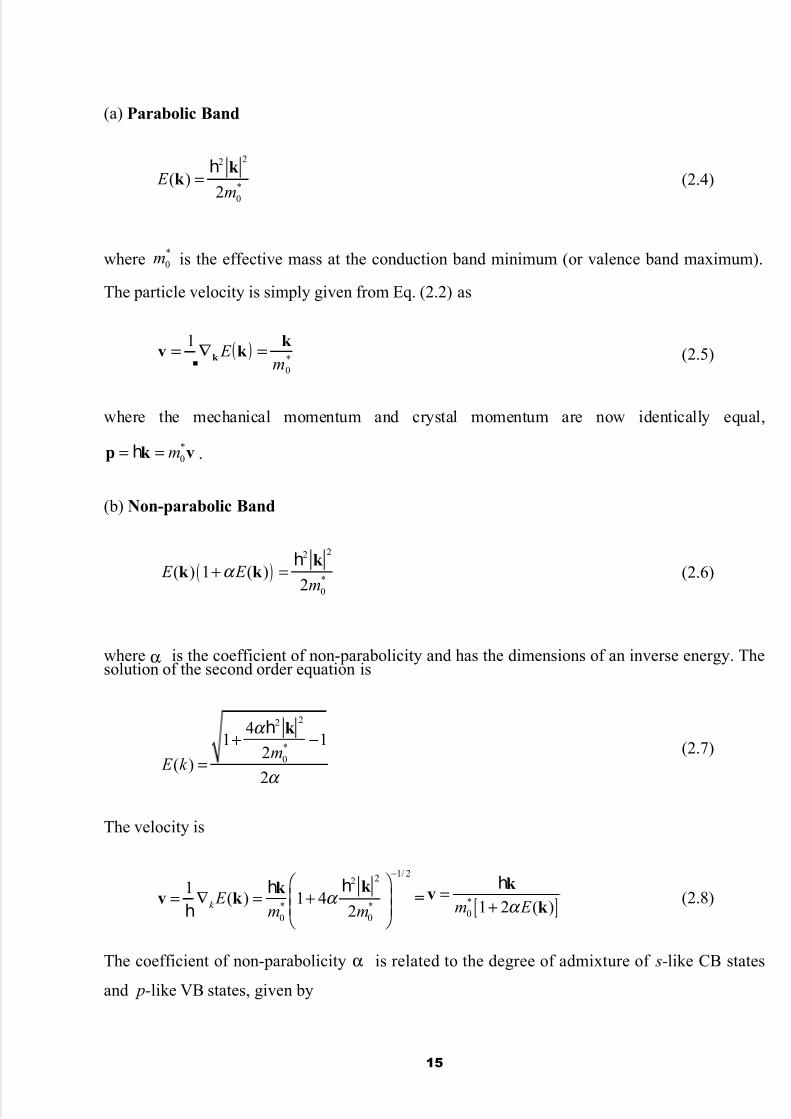
(a) Parabolic Band
22
*
0
( )2
k k E
m=
h(2.4)
where *
0m is the effective mass at the conduction band minimum (or valence band maximum).
The particle velocity is simply given from Eq. (2.2) as
( )*
0
1
m E
k k v k
=∇= (2.5)
where the mechanical momentum and crystal momentum are now identically equal,
*
0p k vm= =h .
(b) Non-parabolic Band
( )22
*
0
( ) 1 ( )2
k k k E E
mα + =
h(2.6)
where α is the coefficient of non-parabolicity and has the dimensions of an inverse energy. Thesolution of the second order equation is
22
*
0
41 1
2( )
2
k
m E k
α
α
+ −=
h(2.7)
The velocity is
1/ 222
* *
0 0
1( ) 1 4
2
k k v k k
E m m
α
−
= ∇ = +
hh
h=
[ ]*
0 1 2 ( )
k v
k m E α =
+h
(2.8)
The coefficient of non-parabolicity α is related to the degree of admixture of s-like CB states
and p-like VB states, given by
15

5/13/2018 eBook.comp Electronics - slidepdf.com
http://slidepdf.com/reader/full/ebookcomp-electronics 16/236
2*
0
0
1
gap
m
m
E α
−
=(2.9)
where m0 is the electron mass in vacuum, and E gap is the energy gap between valence and
conduction band. Hence, smaller bandgap materials have stronger mixing of CB and VB states,
and therefore a stronger non-parabolicity.
2.3.Carrier Dynamics
Under the influence of an external field, Bloch electrons in a crystal change their
wavevector according to the acceleration theorem
( )F
k
=dt
t d
, (2.10)
where F is the external force (i.e. external to the crystal field itself) acting on a particle, and k
plays the role of a pseudo or crystal momentum in the analogy to Newton’s equation of motion.
The effect on the actual velocity or momentum of the particle is, however, not straightforward as
the velocity is related to the group velocity of the wave packet associated with the particle, and is
given by Eq. (2.2), where ( )k n E is one of the dispersion relations from Figure 2.6. As the
particle moves through k -space under the influence of an electric field, for example, its velocitycan be positive or negative, eventually leading to Bloch oscillations if scattering did not limit the
motion. Only near extremum of the bands, for example, at the point in Figure 2.6 for the
valence band, or close to the L point in the conduction band, does the dispersion relation
resemble that of the free electrons, ( ) *2/22 mk E =k . There, the electron velocity is simply
given by */mk v = , and the momentum is k p = , as discussed in the presvious section.
In the case of the valence band, the states are nearly full, and current can only be carried
by the absence of electrons in a particular state, leading to the concept of holes, whose dynamics
are identical to that of electrons except their motion is in the opposite direction of electrons,
hence they behave as positively charged particles. In relation to transport and device behavior,
16

5/13/2018 eBook.comp Electronics - slidepdf.com
http://slidepdf.com/reader/full/ebookcomp-electronics 17/236
these holes are then treated as positively charged particles in the presence of external fields, and
one has to simulate the motion of both electrons and holes.
For device modeling and simulation, different approximate band models are employed.
As long as carriers (electrons and holes) have relatively low energies, they may be treated using
the so called parabolic band approximation, where they simply behave as free particles having
an effective mass. If more accuracy is desired, corrections due to deviation of the dispersion
relation from a quadratic dependence on k may be incorporated in the nonparabolic band model .
If more than one conduction band minimum is important, this model may be extended to a multi-
valley model , where the term valley refers to different conduction minima. Finally, if the entire
energy dispersion is used, one usually referes to the model as full band .
2.4.Effective Mass in SemiconductorsThe effective mass of a semiconductor is obtained by fitting the actual E-k diagram
around the conduction band minimum or the valence band maximum by a parabola. While this
concept is simple enough, the issue turns out to be substantially more complex due to the
multitude and the occasional anisotropy of the minima and maxima. In this section we first
describe the different relevant band minima and maxima, present the numeric values for
germanium, silicon and gallium arsenide and introduce the effective mass for density of states
calculations and the effective mass for conductivity calculations.
Most semiconductors can be described as having one band minimum at k = 0 as well as
several equivalent anisotropic band minima at k ≠ 0. In addition there are three band maxima of
interest which are close to the valence band edge. As an example we consider the band structure
of silicon as shown in the figure below.
17

5/13/2018 eBook.comp Electronics - slidepdf.com
http://slidepdf.com/reader/full/ebookcomp-electronics 18/236
Figure 2.7. E-k diagram within the first Brillouin zone and along the (100) direction.
Shown is the E-k diagram within the first Brillouin zone and along the (100) direction. The
energy is chosen to be to zero at the edge of the valence band. The lowest band minimum at k = 0
and still above the valence band edge occurs at E c,direct = 3.2 eV. This is not the lowest minimum
above the valence band edge since there are also 6 equivalent minima at k = ( x,0,0), (- x,0,0),
(0, x,0), (0,- x,0), (0,0, x), and (0,0,- x) with x = 5 nm-1. The minimum energy of all these minima
equals 1.12 eV = E c,indirect. The effective mass of these anisotropic minima is characterized by a
longitudinal mass along the corresponding equivalent (100) direction and two transverse massesin the plane perpendicular to the longitudinal direction. In silicon the longitudinal electron mass
is me,l * = 0.98 m0 and the transverse electron masses are me,t
* = 0.19 m0, where m0 = 9.11 x 10⁻³¹ kg
is the free electron rest mass. Two of the three band maxima occur at 0 eV. These bands are
referred to as the light and heavy hole bands with a light hole mass of mlh* = 0.16 m0 and a heavy
hole mass of mhh* = 0.46 m0. In addition there is a split-off hole band with its maximum at E v,so =
-0.044 eV and a split-off hole mass of mv,so* = 0.29 m0.
18

5/13/2018 eBook.comp Electronics - slidepdf.com
http://slidepdf.com/reader/full/ebookcomp-electronics 19/236
Figure 2.8. Constant energy surfaces of the conduction band of Ge, Si and GaAs. Note that in the
case of Ge we have 4 conduction band minima, in the case of Si we have 6 conduction band
equivalent valleys and in the case of Ge we have only one constant energy surface at the center
of the Brillouin zone.
Figure 2.9. 3D equienergy surfaces of heavy hole, light hole and split off band in Si for 0 z k = .
The values of the energy band minima and maxima as well as the effective masses for
germanium, silicon and gallium arsenide are listed in Table 2-1 below.
Table 2-1
Name Symbol Germanium Silicon GalliumArsenide
Band minimum at k = 0
Minimum energy E g,direct [eV] 0.8 3.2 1.424Effective mass me
*/m0 0.041 ?0.2? 0.067Band minimum not at k = 0
Minimum energy E g,indirect
[eV]0.66 1.12 1.734
Longitudinal effective mass me,l */m0 1.64 0.98 1.98
Transverse effective mass me,t */m0 0.082 0.19 0.37
Wavenumber at minimum k [1/nm] xxx xxx xxx
Longitudinal direction (111) (100) (111)Heavy hole valence band maximum
at E = k = 0
Effective mass mhh*/m0 0.28 0.49 0.45
Light hole valence band maximum at
k = 0
Effective mass mlh*/m0 0.044 0.16 0.082
Split-off hole valence band maximum
19

5/13/2018 eBook.comp Electronics - slidepdf.com
http://slidepdf.com/reader/full/ebookcomp-electronics 20/236
at k = 0
Split-off band valence band energy E v,so [eV] -0.028 -0.044 -0.34Effective mass mh,so
*/m0 0.084 0.29 0.154m0 = 9.11 x 10⁻³¹ kg is the free electron rest mass.
The effective mass for density of states calculations equals the mass which provides thedensity of states using the expression for one isotropic maximum or minimum or
*3/2
3
8 2( ) , for C e C C g E m E E E E
h
π = − ≥ , (2.11)
for the density of states in the conduction band, and
*3/2
3
8 2( ) , for V h V V g E m E E E E
h
π = − ≤ , (2.12)
for the density of states in the valence band. For instance for a single band minimum described
by a longitudinal mass and two transverse masses the effective mass for density of states
calculations is the geometric mean of the three masses. Including the fact that there are several
equivalent minima at the same energy one obtains the effective mass for density of states
calculations from:
( )1/3* 2 /3
,e dos C l t t m M m m m= (2.13)
where M c is the number of equivalent band minima. For silicon one obtains
me,dos* = (ml mt mt )1/3 = (6)2/3 (0.89× 0.19× 0.19)1/3 m0 = 1.08 m0. (2.14)
The effective mass for conductivity calculation is the mass which is used in conduction
related problems accounting for the detailed structure of the semiconductor. These calculations
include mobility and diffusion constants calculations. Another example is the calculation of the
shallow impurity levels using a hydrogen-like model. As the conductivity of a material is
inversionally proportional to the effective masses, one finds that the conductivity due to multiple
band maxima or minima is proportional to the sum of the inverse of the individual masses,
multiplied by the density of carriers in each band, as each maximum or minimum adds to the
overall conductivity. For anisotropic minima containing one longitudinal and two transverse
effective masses one has to sum over the effective masses in the different minima along the
20

5/13/2018 eBook.comp Electronics - slidepdf.com
http://slidepdf.com/reader/full/ebookcomp-electronics 21/236
equivalent directions. The resulting effective mass for bands which have ellipsoidal constant
energy surfaces is given by:
*
,
31 1 1e cond
l t t
m
m m m
=+ + (2.15)
provided the material has an isotropic conductivity as is the case for cubic materials. For instance
electrons in the X minima of silicon have an effective conductivity mass given by:
me,cond* = 3× (1/ml + 1/mt + 1/mt )-1 = 3× (1/0.89 + 1/0.19 +1/0.19)-1 m0 = 0.26 m0. (2.16)
Table 2-2. Effective mass and energy bandgap of Ge, Si and GaAsName Symbol Germanium Silicon Gallium
Arsenide
Smallest energy bandgap at 300 K E g (eV) 0.66 1.12 1.424Effective mass for density of
states calculations
Electrons me*,dos/m0 0.56 1.08 0.067
Holes mh*,dos/m0 0.29 0.57/0.811 0.47
Effective mass for conductivity
calculations
Electrons me*,cond/m0 0.12 0.26 0.067
Holes mh*,cond/m0 0.21 0.36/0.386
[
22
]
0.34
m0 = 9.11 x 10⁻³¹ kg is the free electron rest mass.
2.5.Semiclassical Transport Theory
To completely specify the operation of a device, one must know the state of each carrier
within the device. If carriers are treated as classical particles, one way of specifying the state of
the carriers is to solve Newton’s equations
( , , ) and ( )
p r
E r p v
d d
e R t t dt dt = − + = , (2.17)
where ( , , )r p R t is a random force function due to impurities or lattice vibrations or other
imperfections in the system. Alternative approach would be to calculate the probability of
finding a carrier with crystal momentum k at position r at time t , given by the distribution
21

5/13/2018 eBook.comp Electronics - slidepdf.com
http://slidepdf.com/reader/full/ebookcomp-electronics 22/236
function f (r,k ,t ), obtained by solving the Boltzmann transport equation (BTE) [23,24,25]. It is
important to note that this theory is based on the following assumptions:
• Electrons and holes are independent particles.
• The system is described by a set of Bloch functions [26,27].
• Particles do not interact with each other, but may be scattered
by impurities, phonons, etc.
• The number of electrons in an elementary volume ∆ V centered
around r, that have wavevectors in the range of d3k centered around k is given by
3
32 ( , , )
8r k
V f t d k
π
∆×
Therefore, once the distribution function is specified, various moments of the distribution
function can give us particle density, current density, energy density, etc. More precisely
1( , ) ( , , )r r k
k
n t f t V
= ∑ , particle density (2.18)
( , ) ( ) ( , , )J r v k r k k
et f t
V = − ∑ , current density (2.19)
1( , ) ( ) ( , , )r k r k
k
W t E f t V
= ∑ , energy density (2.20)
A full quantum-mechanical view to this problem is rather difficult [28,29]. The uncertainty
principle states, for example, that we can not specify simultaneously the position and the
momentum of the particle. Hence, one needs to adopt a coarse-grained average point of view, in
which positions are specified within a macroscopic volume, and momenta are also specified
within some interval. If one tries to go straightforwardly and construct f (r,k ,t ) from the quantum-
mechanical wavefunctions, difficulties arise since f is not necessarily positive definite.
2.5.1. Approximations made for the distribution function
The most difficult problem in device analysis is to calculate the distribution function f (r,k ,t ). To
overcome these difficulties, reasonable guess for the distribution function is often made. Two
most commonly used approaches are:
• Quasi-Fermi level concept.
• Displaced Maxwellian approximation for the distribution function.
22

5/13/2018 eBook.comp Electronics - slidepdf.com
http://slidepdf.com/reader/full/ebookcomp-electronics 23/236
(A) Quasi-Fermi level concept
Under equilibrium conditions 2
inp n= , where n is the electron concentration, p is the hole
concentration and ni is the intrinsic carrier concentration which follows from the use of the
equilibrium distribution functions for electrons and holes, i.e.
1( ) ,
1 expn
F
B
f E E E
k T
= −+
1( ) 1 ( )
1 exp p n
F
B
f E f E E E
k T
= − = −+
. (2.21)
Under non-equilibrium conditions, it may still be useful to represent the distribution functions for
electrons and holes as
1( )
1 expn
Fn
B
f E E E
k T
= −
+
and
1( ) 1 ( )
1 exp p n
Fp
B
f E f E E E
k T
= − =−
+
. (2.22)
Therefore, under non-equilibrium conditions and assuming non-degenerate statistics, we will
have
exp , and exp V Fp Fn C
C V
B B
E E E E n N p N
k T k T
− −= =
, (2.23)
where N C and N V are the effective density of states of the conduction and valence band,respectively [30,31]. The product
2 exp Fn Fp
i
B
E E np n
k T
− =
(2.24)
suggests that the difference E Fn - E Fp is a measure for the deviation from the equilibrium.
However, this can not be correct distribution function since it is even in k , which means that it
suggests that current can never flow in a device. The fact that makes it not so unreasonable is
that average carrier velocities are usually much smaller than the spread in velocity, given by
72 * 10 / for Bk T m cm s≈ m* = m0 (free electron mass).
23

5/13/2018 eBook.comp Electronics - slidepdf.com
http://slidepdf.com/reader/full/ebookcomp-electronics 24/236
Figure 2.10. Energy band profile of a pn-diode under equilibrium and non-equilibrium
conditions. Note that to get the excess electron density (bottom right panel) the electron
quasi-Fermi level must move up (top right panel), thus increasing the probability of state
occupancy. The same is true for the excess hole concentration, where the hole quasi-Fermi
level moves downward.
(B) Displaced Maxwellian Approximation
A better guess for the distribution function f (r,k ,t ) is to assume that the distribution
function retains its shape, but that its average momentum is displaced from the origin. For
example, particularly suitable form to use is [32]
220( , , ) exp exp
2 *r k k k Fn C
d
B B
E E f t
k T m k T
−= − −
h
. (2.25)
24

5/13/2018 eBook.comp Electronics - slidepdf.com
http://slidepdf.com/reader/full/ebookcomp-electronics 25/236
Figure 2.11. Displaced Maxwellian distribution function.
Using this form of the distribution function gives
01( , ) ( , , ) expr r k Fn C
C
k B
E E n t f t N
V k T
−= =
∑
. (2.26)
In the same manner, one finds that the kinetic energy density per carrier is given by
21 3( , ) *
2 2r d Bu t m v k T = +
. (2.27)
The first term on the RHS represents the drift energy due to average drift velocity, and the
second term is the well known thermal energy term due to collisions of carriers with phonons
[33].
Since in both cases, the guess for the non-equilibrium distribution has been guided by the
form of the equilibrium, they are only valid in near-equilibrium conditions. For far-from-
equilibrium conditions, the shape of the distribution function can be rather different [34]. This
necessitates the solution of the Boltzmann transport equation that is introduced in the following
section.
25

5/13/2018 eBook.comp Electronics - slidepdf.com
http://slidepdf.com/reader/full/ebookcomp-electronics 26/236
2.6.Boltzmann transport equation
To derive the BTE consider a region of phase space about the point( , , , , , ) x y z x y z p p p
. The
number of particles entering this region in time dt is equal to the number which were in the
region of phase space ( x-v xdt,y-v ydt,z-v z dt,p x-F xdt,p y-F ydt,p z -F z dt ) at a time dt earlier. If
f ( x,y,z,p x ,p y ,p z ) is the distribution function which expresses the number of particles per quantum
state in the region, then the change d f which occurs during time dt due to the motion of the
particles in coordinate space and due to the fact that force fields acting on the particles tend to
move them from one region to another in momentum space is [35]:
( , , , , , )
( , , , , , )
x y z x x y y z z
x y z
df f x v dt y v dt z v dt p F dt p F dt p F dt
f x y z p p p
= − − − − − −
−(2.28)
Using Taylor series expansion, we get
r pv F
df f f
dt = − ⋅∇ − ⋅∇
(2.29)
So far, only the change in the distribution function due to the motion of particles in coordinate
space and due to the momentum changes arising from the force fields acting on the particles have
been accounted for. Particles may also be transferred into or out of a given region in phase space
by collisions or scattering interactions involving other particles of the distribution or scattering
centers external to the assembly of particles under consideration. If the rate of change of the
distribution function due to collisions, or scattering, is denoted by ( )coll
f t ∂ ∂, the total rate of
change of f becomes
( , , )r pv Fcoll
df f f f s r p t dt t
∂= − ⋅∇ − ⋅∇ + +∂ (2.30)
i.e.
26

5/13/2018 eBook.comp Electronics - slidepdf.com
http://slidepdf.com/reader/full/ebookcomp-electronics 27/236
( , , )r p+v F
coll
df f f f s r p t
dt t
∂⋅∇ + ⋅∇ = +
∂ (2.31)
The last term on the RHS of Eqs. (3.14) and (3.15) occurs when generation-recombination
processes play significant role. Eq. (3.15) represents the Boltzmann transport equation, which is
nothing more but a book-keeping equation for the particle flow in the phase space.
Figure 2.12. A cell in two-dimensional phase space. The three processes, namely drift,
diffusion, and scattering, that affect the evolution of f(r,p,t) with time in phase space are
shown.
The various terms that appear in Eq. (2.31) represent
•( ) pF
forces f t f ∂ ∂ = − ⋅∇
, where( )p k F E v Bd d q
dt dt = = = + ×h
, the total force equals
the sum of the force due to the electric field and the Lorentz force due to the magnetic
flux density, B.
27

5/13/2018 eBook.comp Electronics - slidepdf.com
http://slidepdf.com/reader/full/ebookcomp-electronics 28/236
•( ) rv
diff f t f ∂ ∂ = − ⋅∇
. This term arises if there is a spatial variation in the distribution
function due to concentration or temperature gradients, both of which will result in a
diffusion of carriers in coordinate space.
• ( ) coll f t ∂ ∂ is the collision term which equals the difference between the in-scattering
and the out-scattering processes, i.e.
[ ] [ ] '
( ', ) ( ') 1 ( ) ( , ') ( ) 1 ( ')k k k k k k k k k coll
f S f f S f f Cf
t
∂ = − − − = ∂ ∑
)
(2.32)
The presence of f (k ) and f (k’) in the collision integral makes the BTE rather complicated
integro-differential equation for f (r,k ,t ), whose solution requires a number of simplifying
assumptions. In the absence of perturbing fields and temperature gradients, the distribution
function must be the Fermi-Dirac function. In this case, the collision term must vanish and the
principle of detailed balance gives for all k and k ’ and all scattering mechanisms
[ ]
[ ]0 0
0 0
( ') 1 ( )( , ')
( ', ) ( ) 1 ( ')
k k k k
k k k k
f f S
S f f
−=
−. (2.33)
Therefore, if the phonons interacting with the electrons are in thermal equilibrium, we get
( , ')exp
( ', )k k'k k
k k B
E E S
S k T
−=
. (2.34)
This relation must be satisfied regardless of the origin of the scattering forces. If, for example,
we assume k k' E E > , then ( , ')k k S which involves emission must exceed ( ', )k k S which
involves absorption. Note that the BTE is valid under assumptions of semi-classical transport:
effective mass approximation (which incorporates the quantum effects due to the periodicity of
the crystal); Born approximation for the collisions, in the limit of small perturbation for the
electron-phonon interaction and instantaneous collisions; no memory effects, i.e. no dependence
on initial condition terms. The phonons are usually treated as in equilibrium, although the
condition of non-equilibrium phonons may be included through an additional equation [36].
28

5/13/2018 eBook.comp Electronics - slidepdf.com
http://slidepdf.com/reader/full/ebookcomp-electronics 29/236
2.7.Scattering Processes
Free carriers (electrons and holes) interact with the crystal and with each other through a
variety of scattering processes which relax the energy and momentum of the particle. Based on
first order, time-dependent perturbation theory, the transition rate from an initial state k in bandn to a final state k ’ in band m for the jth scattering mechanism is given by Fermi’s Golden rule
[37]
[ ] ( ) ( )ω δ π
k k k rk k k E E nV mmn j j −′=′Γ ′
2
,,2
,;, (2.35)
where V j(r) is the scattering potential of this process, E k and E k ’ are the initial and final state
energies of the particle. The delta function describes conservation of energy, valid for long timesafter the collision is over, with ω the energy absorbed (upper sign) or emitted (lower sign)
during the process. The total rate used to generate the free flight in Eq. (6.5), discussed
previously, is then given by
[ ] ( ) ( )∑′
′ −′=Γ k
k k k rk k
,
2
,,2
,m
j j E E nV mn ω δ π
. (2.36)
There are major limitations to the use of the Golden rule due to effects such as collision
broadening and finite collision duration time [85]. The energy conserving delta function is only
valid asymptotically for times long after the collision is complete. The broadening in the final
state energy is given roughly by τ ≈∆ E , where τ is the time after the collision, which
implies that the normal E (k ) relation is only recovered at long times. Attempts to account for
such collision broadening in Monte Carlo simulation have been reported in the literature [38,39],
although this is still an open subject of debate. Inclusion of the effects of finite collision
duration in Monte Carlo simulation have also been proposed [40
,41
]. Beyond this, there is still the problem of dealing with the quantum mechanical phase coherence of carriers, which is neglected
in the scatter free-flight algorithm of the Monte Carlo algorithm, and goes beyond the semi-
classical BTE description.
29

5/13/2018 eBook.comp Electronics - slidepdf.com
http://slidepdf.com/reader/full/ebookcomp-electronics 30/236
Scattering Mechanisms
Defect Scattering Carrier-Carrier Scattering Lattice Scattering
Crystal
DefectsImpurity Alloy
Neutral Ionized
Intravalley Intervalley
Acoustic OpticalAcoustic Optical
Nonpolar Polar Deformation
potential
Piezo-
electric
Scattering Mechanisms
Defect Scattering Carrier-Carrier Scattering Lattice Scattering
Crystal
DefectsImpurity Alloy
Neutral Ionized
Intravalley Intervalley
Acoustic OpticalAcoustic OpticalAcoustic Optical
Nonpolar Polar Nonpolar Polar Deformation
potential
Piezo-
electric
Figure 2.13. Scattering mechanisms in a typical semiconductor.
Figure 2.13 lists the scattering mechanisms one should in principle consider in a typical
Monte Carlo simulation. They are roughly divided into scattering due to crystal defects, which is
primarily elastic in nature, lattice scattering between electrons (holes) and lattice vibrations or
phonons, which is inelastic, and finally scattering between the particles themselves, including
both single particle and collective type excitations. Phonon scattering involves different modes
of vibration, either acoustic or optical, as well as both transverse and longitudinal modes.Carriers may either emit or absorb quanta of energy from the lattice, in the form of phonons, in
individual scattering events. The designation of inter- versus intra-valley scattering comes from
the multi-valley band-structure model of semiconductors discussed in Section 2.2, and refers to
whether the initial and final states are in the same valley or in different valleys. The scattering
rates [ ]k k ′Γ ,;, mn j and [ ]k ,n jΓ are calculated using time dependent perturbation theory
using Fermi’s rule, Eqs. (2.35) and (2.36), and the calculated rates are then tabulated in a
scattering table in order to select the type of scattering and final state after scattering as discussedearlier.
30

5/13/2018 eBook.comp Electronics - slidepdf.com
http://slidepdf.com/reader/full/ebookcomp-electronics 31/236
2.8.Relaxation-time approximation
Analytical solutions of the Boltzmann equation are possible only under very restrictive
assumptions [42]. Direct numerical methods for device simulation have been limited by the
complexity of the equation, which in the complete 3-D time-dependent form requires sevenindependent variables for time, space and momentum. In recent times, more powerful
computational platforms have spurred a renewed interest in numerical solutions based on the
spheroidal harmonics expansion of the distribution function [43]. To-date, most semiconductor
applications have been based on stochastic solution methods (Monte Carlo), which involve the
simulation of particle trajectories rather than the direct solution of partial differential equations.
Most conventional device simulations are based on approximate models for transport
which are derived from the Boltzmann equation, coupled to Poisson's equation for self-
consistency. In the simplest approach, the relaxation time approximation is invoked, where the
total distribution function is split into a symmetric term in terms of the momentum (which is
generally large) and an asymmetric term in the momentum (which is small). In other words,
( , , ) ( , , ) ( , , )r k r k r k S A f t f t f t = + . (2.37)
Then, for non-degenerate semiconductors (1 - f ) ≈ 1, the collision integral Eq. (3.16) may be
written
[ ]
( )
[ ]( )
[ ]'
''
( ') ( ', ) ( ) ( , ')
( ') ( ', ) ( ) ( , ')( ') ( ', ) ( ) ( , ')
k
k k
k k k k k k
k k k k k k k k k k k k
AS coll coll f t f t
coll
A AS S
f f S f S
t
f S f S f S f S
∂ ∂∂ ∂
= +
∂ = − ∂
−− ∑∑
∑
(2.38)
We now consider two cases:
(a) Equilibrium conditions:0 , 0 0S
S A
coll coll
f f f f f
t t
∂∂ = = → = = ∂ ∂
(b) Non-equilibrium conditions when 0 A f ≠ . In this case, we must consider two different
situations:
31

5/13/2018 eBook.comp Electronics - slidepdf.com
http://slidepdf.com/reader/full/ebookcomp-electronics 32/236
- Low-field conditions, where S f retains its equilibrium form with C LT T = . In this case
( ) 0S coll f t ∂ ∂ =
.
- High-field conditions whenC LT T ≠
andS f
does not retain its equilibrium form. In
this case ( ) 0S coll f t ∂ ∂ ≠
.
In all of these cases, a plausible form for the term ( ) A coll f t ∂ ∂
is
A A
coll f
f f
t τ
∂ = − ∂ , (2.39)
where f τ
is a characteristic time that describes how the distribution function relaxes to its
equilibrium form. With the above discussion, we may conclude that
- At low fields:
A A
coll coll f
f f f
t t τ
∂∂ = = − ∂ ∂ .
- At high fields:
S S A A
coll coll coll coll f
f f f f f
t t t t τ
∂ ∂∂∂ = + = − ∂ ∂ ∂ ∂ .
To understand the meaning of the relaxation time, we consider a semiconductor in which there
are no spatial and momentum gradients. With the gradient terms zero, the BTE becomes
0 A A
scatt f f
f f f f f
t t τ τ
−∂∂ = = − = − ∂ ∂ (2.40)
i.e.
0
f f
f f f
t τ τ
∂+ =
∂(2.41)
The solution of this first-order differential equation is
32

5/13/2018 eBook.comp Electronics - slidepdf.com
http://slidepdf.com/reader/full/ebookcomp-electronics 33/236
[ ]/
0 0( ) (0) f t f t f f f e
τ −= + −. (2.42)
This result suggests that any perturbation in the system will decay exponentially with a
characteristic time constant f τ . It also suggests that the RTA is only good when [ ]0(0) f f − is
not very large. Note that an important restriction for the relaxation-time approximation to be
valid is that f τ is independent of the distribution function and the applied electric field.
2.9.Solving the BTE in the Relaxation Time Approximation
Let us consider the simple case of a uniformly doped semiconductor with a constant electric field
throughout. Since there are no spatial gradients, 0r f ∇ = . Under steady-state conditions we also
have 0 f t ∂ ∂ = . With the above simplifications, the BTE reduces to
1p k F F
coll
f f f
t
∂ ⋅∇ = ⋅∇ = ∂ h (2.43)
For parabolic bands and choosing the coordinate system such that the electric field is along the z -
axis, one can expand the distribution function into Legendre polynomials
0
1
( , ) ( , ) ( ) (cos )n n
n
f z p f z p g E P θ ∞
=
= + ∑(2.44)
where 0 1 P = , 1 cos P θ = ,23 1
2 2 2cos P θ = − , … . In the above expressions, θ is the angle between
the applied field (along the symmetry axis), and the momentum of the carriers. For sufficiently
low fields, we expect that only the lowest order term is important, so that
0 1 0( ) ( ) ( ) cos ( ) ( ) A f p f p g p f p f pθ ≅ + = + . (2.45)
Substituting the results on the LHS of the BTE and using parabolic dispersion relation gives
33

5/13/2018 eBook.comp Electronics - slidepdf.com
http://slidepdf.com/reader/full/ebookcomp-electronics 34/236
[ ]0 1
0 00
( ) ( ) cos
( ) cos
k
k
E
E E v
e LHS f p g p
f f e f p e eEv
θ
θ ε ε
= − ⋅∇ +
∂ ∂≈ − ⋅∇ = − ⋅ = −
∂ ∂
h
h (2.46)
where, as previously noted θ is the angle between the electric field and v.
We now consider the collision integral on the RHS of the BTE given in Eq. (2.43).
Substituting the first order approximation for f (p) gives
[ ]
[ ]
0 0
'
1 1'
11
' 1
0 11
' 0 1
( ', ) ( ') ( , ') ( )
( ', ) ( ') cos ' ( , ') ( ) cos
( ', ) ( ') cos '( ) cos ( , ') 1
( , ') ( ) cos
( ) ( ') cos '( ) cos ( , ') 1
( ') ( )cos
k coll
k
k
k
f S k k f k S k k f k
t
S k k g k S k k g k
S k k g k g k S k k
S k k g k
f k g k g k S k k
f k g k
θ θ
θ θ
θ
θ θ
θ
∂= −
∂
+ −
= − −
= − −
∑
∑∑
∑(2.47)
where in the last line of the derivation we have used the principle of detailed balance. We can
further simplify the above result, by considering the following coordinate system:
Figure 2.14. Coordinate system used in the rest of the derivation.
Within this coordinate system, we have:
34
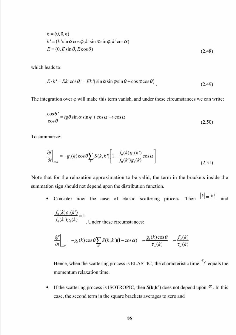
5/13/2018 eBook.comp Electronics - slidepdf.com
http://slidepdf.com/reader/full/ebookcomp-electronics 35/236
(0, 0, )
' ( 'sin cos , 'sin sin , 'cos )
(0, sin , cos )
k k
k k k k
E E E
α ϕ α ϕ α
θ θ
=== (2.48)
which leads to:
( )' 'cos ' ' sin sin sin cos cos E k Ek Ek θ α ϕ θ α θ ⋅ = = +. (2.49)
The integration over φ will make this term vanish, and under these circumstances we can write:
cos 'sin sin cos cos
costg
θ θ α ϕ α α
θ = + →
(2.50)
To summarize:
0 11
' 0 1
( ) ( ')( ) cos ( , ') 1 cos
( ') ( )k coll
f k g k f g k S k k
t f k g k θ α
∂= − − ∂
∑(2.51)
Note that for the relaxation approximation to be valid, the term in the brackets inside the
summation sign should not depend upon the distribution function.
• Consider now the case of elastic scattering process. Then 'k k = and
0 1
0 1
( ) ( ')1
( ') ( )
f k g k
f k g k =
. Under these circumstances:
11
'
( ) cos ( )( )cos ( , ')(1 cos )
( ) ( ) A
k coll m m
g k f k f g k S k k
t k k
θ θ α
τ τ
∂= − − = − = −
∂ ∑
Hence, when the scattering process is ELASTIC, the characteristic time f τ equals the
momentum relaxation time.
• If the scattering process is ISOTROPIC, then S (k ,k’) does not depend upon α . In this
case, the second term in the square brackets averages to zero and
35

5/13/2018 eBook.comp Electronics - slidepdf.com
http://slidepdf.com/reader/full/ebookcomp-electronics 36/236
11
'
( )cos ( )( )cos ( , ')
( ) ( ) A
k coll
g k f k f g k S k k
t k k
θ θ
τ τ
∂= − = − = −
∂ ∑
Thus, in this case, the characteristic time is the scattering time or the average time
between collision events.
To summarize, under low-field conditions, when the scattering process is either isotropic or
elastic, the collision term can be represented as/ ( ) A f f k τ −
, where in general( ) f k τ
is the
momentum relaxation time that depends only upon the nature of the scattering process.
Following these simplifications, the BTE can thus be written as
0 1( ) coscos( )m
f g k eEv E k
θ θ τ ∂ − = − ∂ (2.52)
or
01( ) ( )m
f g k eEv k
E τ
∂ = ∂ (2.53)
The distribution function is, thus, equal to
00
00
( ) ( ) cos ( )
( ) ( )
m
z m
f f k f k eEv k
E
f f k eEv k
E
θτ
τ
∂ = + ∂ ∂ = + ∂ (2.54)
To further investigate the form of this distribution function, we use
0 01
z z
f f
E v k
∂ ∂=
∂ ∂h . This leads to
00( ) ( ) ( )m
z
f e f k f k E k
k τ
∂= +
∂h (2.55)
36

5/13/2018 eBook.comp Electronics - slidepdf.com
http://slidepdf.com/reader/full/ebookcomp-electronics 37/236
The second term of the last expression resembles the linear term in the Taylor series expansion
of f (k ). Hence, we can write
0( , , ) , , ( ) x y z x y z m
e f k k k f k k k E k τ
= + h (2.56)
To summarize, the assumption made at arriving at this last result for displaced Maxwellian form
for the distribution function is that the electric field E is small. Hence, the displaced Maxwellian
is a good representation of the distribution function under low-field conditions [ Error: Reference
source not found].
Problems:
1. Electrons in a lattice see a periodic potential due to the presence of the atoms, which is of theform shown below:
a
This periodic potential will open gaps in the dispersion relation, i.e. it will impose limits onthe allowed particle energies. To simplify the problem, one can assume that the width of the potential energy term goes to zero, i.e. the periodic potential can be represented as an infiniteseries of δ -function potentials:
x
V ( x)
a
V 0
(1) (2)
(a) Using Bloch theorem for the general form of the solution of the 1D TISE (time-independent Schrödinger equation) in the presence of periodic potential, show that therelationship between the crystal momentum and particle energy is obtained by solving thefollowing implicit equation
cos( )sin( )
cos( )ka P k a
k ak a= +0
0
0 ,
37

5/13/2018 eBook.comp Electronics - slidepdf.com
http://slidepdf.com/reader/full/ebookcomp-electronics 38/236
where k is the crystal momentum and mk E 220
2= . The quantity P mV = 2 0
2 in the
above equation may be regarded as the "scattering power" of a single potential spike.
(b) Plot the dispersion relation for a particle in a periodic potential for the case when P=2.5 .
2. In the free-electron approximation, the total energy of the electrons is assumed to be alwayslarge compared to the periodic potential energy. Writing the 1D time-independentSchrödinger wave equation in the form
[ ] 0)()(202
2
=ψ γ ++ψ
x x f k dx
d ,
where mk E 220
2= and 2/)(2)( xmV x f =γ , it is rather straightforward to show that in
the limit 0→γ and away from the band edge points ( an /π± ), one can approximate thewavefunction )( xψ with
anxi
n
nikxikxanxi
n
nikx
k ikx ebeebebe xue x /2
0
0/2)()( π−
≠
π− ∑γ +≈∑==ψ .
(a) Show that the result given above is a valid approximation for )( xψ in the limit 0→γ and away from the band-edge points.
(b) Find the relationship between the expansion coefficients nb and the Fourier expansioncoefficients for the periodic potential )( xV for this case. Also, obtain an analyticexpression for the dispersion relation (the relationship between the allowed particleenergies and the crystal momentum k ) for values of the crystal momentum away from the band-edge points.
(c) How will the results from parts (a-c) change if the crystal momentum approaches the
band edge points ank n /π±= ? What is the appropriate approximate expression for thewavefunction in this case? Evaluate the dispersion relation in the vicinity of the bandedge points and discuss the overall energy-wavevector dispersion relation in the free-electron approximation.
3. In the free-electron approximation, discussed in problem 2, it was assumed that the potentialenergy of the electron is small compared to its total energy. The atoms are assumed to bevery close to each other, so that there is significant overlap between the wavefunctions for the electrons associated with neighboring atoms. This leads to wide energy bands and verynarrow energy gaps. The tight-binding approximation proceeds from the opposite limit, i.e.it assumes that the potential energy of the electron accounts for nearly all of the total energy.
The atoms are assumed to be very far apart so that the wavefunctions for the electronsassociated with neighboring atoms overlap only to a small extent. A brief description of thetight-binding method is given below:
If the potential function associated with an isolated atom is )(0 rV , then the solution of the Schrödinger equation
38

5/13/2018 eBook.comp Electronics - slidepdf.com
http://slidepdf.com/reader/full/ebookcomp-electronics 39/236
)()()(2
)(ˆ0000
22
00 rrrr ψ =ψ
+∇−=ψ E V
m H
,
describes the electronic wavefunctions of the atom. If the ground-state wavefunction is notmuch affected by the presence of the neighboring atoms, then the crystal wavefunction is
given by:)()( 0 n
n
i ne rrrrk −ψ ∑=ψ ⋅
,
and the periodic potential is represented as
)()( 0 nn
V V rrr −∑= ,
where rn is a vector from some reference point in space to a particular lattice site. Now, if weexpress the potential energy term in the total Hamiltonian of the system as
)(')()()()()( 000 rrrrrrrrr H V V V V V nnn +−=−−+−= ,it is rather straightforward to show that the expectation value of the energy of the system isgiven by
[ ] )()()()(1
00*00 rrrrr
rk ψ ∫ −−ψ ∑+= ⋅−V V dV e
N E E m
m
i m . (P2.1)
where N is the number of atoms in the crystal.
(a) Complete the derivation that leads to the result given in (P2.1).(b) If we assume that the atomic wavefunctions are spherically symmetric ( s-type), show that
in the case then the nearest-neighbor interaction are only taken into account, the energy
of the system for simple cubic lattice is of the form( ) ( )ak ak ak E E z y x coscoscos20 ++β−α−= .
Identify the meaning of the terms α and β in the result given above. What is theapproximate form of the dispersion relation for an electron moving in the x-direction withmomentum ak x /π<< .
(c) Find the dispersion relation for an s-band in the tight-binding approximation for a body-centered and face-centered cubic crystal in the tight-binding approximation, consideringoverlap of nearest-neighbor wavefunctions only.
(d) Plot the form of the forms of the constant energy surfaces for several energies within thezone. Show that these surfaces are spherical for energies near the bottom of the band.
(e) Show that E k ∇⋅n vanishes on the zone boundaries.
39

5/13/2018 eBook.comp Electronics - slidepdf.com
http://slidepdf.com/reader/full/ebookcomp-electronics 40/236
3. The Drift-Diffusion Equations and Their Numerical Solution
In Chapter 1, we discussed the various levels of approximations that are employed in the
modeling of semiconductor devices, and then looked at the semi-classical description of charge
transport via the Boltzmann Transport Equation in Chapter 2. However, the direct solution of
the full BTE is challenging computationally, particularly when combined with field solvers for
device simulation. Therefore, for traditional semiconductor device modeling, the predominant
model corresponds to solutions of the so-called drift-diffusion equations, which are ‘local’ in
terms of the driving forces (electric fields and spatial gradients in the carrier density), i.e. thecurrent at a particular point in space only depends on the instantaneous electric fields and
concentration gradient at that point. The present chapter is devoted to the drift-diffusion model
and its application to semiconductor device modeling. We first look at the derivation of the
drift-diffusion model from the BTE, and the physical significance of the parameters associated
with these equations. We then look at the numerical solution of the drift-diffusion equations
coupled with Poisson’s equation in the domain of the semiconductor, leading to the Sharfetter-
Gummel algorithm which is widely used in conventional device simulation.
3.1.Drift-diffusion model
The popular drift-diffusion current equations can be easily derived directly from the
Boltzmann transport equation. Let us consider a steady state situation and for simplicity a 1-D
geometry. With the use of a relaxation time approximation as in Eq. (3.33), the Boltzmann
transport equation becomes [44]
0 ( , )
*
f f v xeE f f v
m v x τ
−∂ ∂+ =
∂ ∂ . (3.57)
40

5/13/2018 eBook.comp Electronics - slidepdf.com
http://slidepdf.com/reader/full/ebookcomp-electronics 41/236
In writing Eq. (3.1) parabolic band approximation has been assumed and the charge e has to be
taken with the proper sign of the particle (positive for holes and negative for electrons). A
general definition of current density is given in Eq. (2.19) and is repeated here for completeness
( ) ( , ) J x e vf v x dv= ∫ (3.58)
where the integral on the right hand side represents the first ‘moment’ of the distribution
function. This definition of current can be related to Eq. (3.1) after multiplying both sides by v
and integrating over v. From the RHS of Eq. (3.1) we get
0
1 ( )( , )
J xvf dv vf v x dv
eτ τ − = − ∫ ∫
(3.59)
The equilibrium distribution function is symmetric in v, and its integral is zero. Therefore, we
have
2( ) ( , )*
e f d J x e E v dv e v f v x dv
m v dx
τ τ
∂= − −
∂∫ ∫ (3.60)
Integrating by parts we have
[ ]( , ) ( , ) ( ) f
v dv vf v x f v x dv n xv
∞
−∞
∂= − = −
∂∫ ∫ (3.61)
and we can write
2 2( , ) ( )v f v x dv n x v=∫ (3.62)
where2v
is the average of the square of the velocity. The drift-diffusion equations are derived
introducing the mobility *
e
m
τ µ =
and replacing2v
with its average equilibrium value * Bk T
m for
41

5/13/2018 eBook.comp Electronics - slidepdf.com
http://slidepdf.com/reader/full/ebookcomp-electronics 42/236
a 1D case and
3
* Bk T
m for a 3D case, therefore neglecting thermal effects. The diffusion coefficient
D is also introduced, and the resulting drift-diffusion current expressions for electrons and holes
are
( ) ( )
( ) ( )
n n n
p p p
dn J qn x E x qD
dx
dn J qp x E x qD
dx
µ
µ
= +
= −(3.63)
respectively, where q is used to indicate the absolute value of the electronic charge. Although no
direct assumptions on the non-equilibrium distribution function f (v, x) was made in the derivation
of Eqs. (45), in effect, the choice of equilibrium (thermal) velocity means that the drift-diffusionequations are only valid for very small perturbations of the equilibrium state (low fields). The
validity of the drift-diffusion equations is empirically extended by introducing field-dependent
mobility ( ) E µ and diffusion coefficient D(E), obtained from empirical models or detailed
calculation to capture effects such as velocity saturation at high electric fields due to phonon
scattering. A more detailed description of the most commonly used models for the carrier
mobility is given in Appendix B.
3.1.1. Physical Limitations on Numerical Drift-Diffusion Schemes
The complete drift-diffusion model is based on the following set of equations:
1. Current equations
( ) ( )
( ) ( )
n n n
p p p
dn J qn x E x qD
dx
dn J qp x E x qD dx
µ
µ
= +
= − (3.64)
2. Continuity equations
42

5/13/2018 eBook.comp Electronics - slidepdf.com
http://slidepdf.com/reader/full/ebookcomp-electronics 43/236
1
1
J
J
n n
p p
nU
t q
pU
t q
∂= ∇⋅ +
∂∂
= − ∇ ⋅ +∂ (3.65)
3. Poisson's equation
( ) D AV p n N N ε + −∇ ⋅ ∇ = − − + −
(3.66)
where U n and U p are the net generation-recombination rates. The continuity equations are the
conservation laws for the carriers. A numerical scheme which solves the continuity equations
should
1. Conserve the total number of particles inside the device being simulated.
2. Respect local positive definite nature of carrier density. Negative density is unphysical.
3. Respect monotonicity of the solution (i.e. it should not introduce spurious space
oscillations).
Conservative schemes are usually achieved by subdivision of the computational domain into
patches (boxes) surrounding the mesh points. The currents are then defined on the boundaries of
these elements, thus enforcing conservation (the current exiting one element side is exactly equal
to the current entering the neighboring element through the side in common). For example, on a
uniform 2-D grid with mesh size ∆ , the electron continuity equation could be discretized in an
explicit form as follows [45]
1 1 1 12 2 2 2
( , ; ) ( , ; ) ( , ; ) ( , ; )( , ; 1) ( , , ) x x y x J i j k J i j k J i j k J i j k n i j k n i j k
t q q
+ − − + − −+ −= +
∆ ∆ ∆ (3.67)
In Eq. (3.11), the indices i,j describe spatial discretization, k corresponds to the time progression,
and the superscripts x and y denote the x- and y-coordinate of the current density vector. This
simple approach has certain practical limitations, but is sufficient to illustrate the idea behind the
conservative scheme. With the present convention for positive and negative components, it is
easy to see that in the absence of generation-recombination terms, the only contributions to the
43

5/13/2018 eBook.comp Electronics - slidepdf.com
http://slidepdf.com/reader/full/ebookcomp-electronics 44/236
overall device current arise from the contacts. Remember that, since electrons have negative
charge, the particle flux is opposite to the current flux. The actual determination of the current
densities appearing in Eq. (3.11) will be discussed later. When the equations are discretized,
using finite differences for instance, there are limitations on the choice of mesh size and time
step [46]:
1. The mesh size x∆ is limited by the Debye length.
2. The time step is limited by the dielectric relaxation time.
A mesh size must be smaller than the Debye length where one has to resolve charge variations in
space. A simple example is the carrier redistribution at an interface between two regions with
different doping levels. Carriers diffuse into the lower doped region creating excess carrier distribution which at equilibrium decays in space down to the bulk concentration with
approximately exponential behavior. The spatial decay constant is the Debye length
2 B
Dk T
Lq N
ε =
(3.68)
where N is the doping density. In GaAs and Si, at room temperature the Debye length is
approximately 400 Å when 16 310 N cm−≈ and decreases to about only 50 Å when 18 310 N cm−≈ .
The dielectric relaxation time is the characteristic time for charge fluctuations to decay
under the influence of the field that they produce. The dielectric relaxation time may be
estimated using
dr t qN
ε
µ =
(3.69)
To see the importance of respecting the limitations related to the dielectric relaxation time,
imagine we have a spatial fluctuation of the carrier concentration, which relaxes to equilibrium
according to the rate equation
44

5/13/2018 eBook.comp Electronics - slidepdf.com
http://slidepdf.com/reader/full/ebookcomp-electronics 45/236
( 0)
dr
n n t
t t
∂∆ ∆ == −
∂ (3.70)
A finite difference discretization of this equation gives at the first time step
( )(0)
(0)dr
t nn t n
t
∆ ∆∆ ∆ = ∆ −
(3.71)
Clearly, if dr t t ∆ > , the value of ( )n t ∆ ∆ is negative, which means that the actual concentration is
evaluated to be less than the equilibrium value, and it is easy to see that the solution at higher
time steps will decay oscillating between positive and negative values of n∆ . An excessively
large t ∆ may lead, therefore, to nonphysical results. In the case of high mobility the dielectric
relaxation time can be very small. For instance, a sample of GaAs with a mobility of
26000 /cm V s− and doping18 310 cm−
has approximately1510dr t s−≈ , and in a simulation the
time step t ∆ should be chosen to be considerably smaller.
3.1.2. Steady State Solution of Bipolar Semiconductor Equations
The general semiconductor equations may be rewritten in 3D as
( ) ( )
( , )
( , )
B
n
p
Bn n
B p p
V q n p N
n J qU n p q
t
p J qU n p q
t
k T J q n V n
q
k T J q p V pq
ε
µ
µ
∇ ⋅ ∇ = − +
∂∇ ⋅ = +
∂∂
∇ ⋅ = − +∂
= − ∇ + ∇
= − ∇ − ∇ (3.72)
with B A D N N N = − . Note that the above equations are valid in the limit of small deviations from
equilibrium, since the Einstein relations have been used for the diffusion coefficient, normally
valid for low fields or large devices. The generation-recombination term U will be in general a
45

5/13/2018 eBook.comp Electronics - slidepdf.com
http://slidepdf.com/reader/full/ebookcomp-electronics 46/236
function of the local electron and hole concentrations, according to possible different physical
mechanisms, to be examined later in more detail. We will consider from now on steady state,
with the time dependent derivatives set to zero.
These semiconductor equations constitute a coupled nonlinear set. It is not possible, in
general, to obtain a solution directly in one step, but a nonlinear iteration method is required. The
two more popular methods for solving the discretized equations are the Gummel's iteration
method [47] and the Newton's method [48]. It is very difficult to determine an optimum strategy
for the solution, since this will depend on a number of details related to the particular device
under study. There are in general three possible choices of variables.
1. Natural variable formulation (V ,n, p)
2. Quasi-Fermi level formulation( , , )n pV φ φ
, where the quasi-Fermi levels derive from the
following definition of carrier concentration out of equilibrium (for non-degenerate case)
( )exp
( )exp
ni
B
p
i
B
q V n n
k T
q V p n
k T
φ
φ
−=
−
=
3. Slotboom formulation( ), ,n pV Φ Φ
where the Slotboom [49] variables are defined as
exp
exp
nn i
B
p
p i
B
qn
k T
qn
k T
φ
φ
Φ = −
Φ =
The Slotboom variables are, therefore, related to the carrier density expressions, and the
extension to degenerate conditions is cumbersome.
Normally, there is a preference for the quasi-Fermi level formulation in steady state simulation,
and for the natural variables n and p in transient simulation.
46

5/13/2018 eBook.comp Electronics - slidepdf.com
http://slidepdf.com/reader/full/ebookcomp-electronics 47/236
3.1.3. Normalization and Scaling
For the sake of clarity, all formulae have been presented without the use of
simplifications or normalization. It is however common practice to perform the actual calculation
using normalized units to make the algorithms more efficient, and in cases to avoid numericaloverflow and underflow. It is advisable to input the data in M.K.S. or practical units (the use of
centimeters is for instance very common in semiconductor practice, instead of meters) and then
provide a conversion block before and after the computation blocks to normalize and
denormalize the variables. It is advisable to use consistent scaling, rather than set certain
constants to arbitrary values. The most common scaling factors for normalization of
semiconductor equations are listed in Table 3-3 [50].
Table 3-3. Scaling factors
Variable Scaling Variable FormulaSpace Intrinsic Debye length ( N=ni)
Extrinsic Debye length ( N=N max)
2
Bk T
Lq N
ε =
Potential Thermal voltage* Bk T
V q
=
Carrier
concentration
Intrinsic concentration
Maximum doping concentration
N=ni
N=N max
Diffusion
coefficient
Practical unit
Maximum diffusion coefficient
2
1cm
D s
=
D = Dmax
Mobility
*
DM
V =
Generation-
Recombination
2
DN R
L=
Time 2 LT
D=
47

5/13/2018 eBook.comp Electronics - slidepdf.com
http://slidepdf.com/reader/full/ebookcomp-electronics 48/236
3.1.4. Gummel's Iteration Method
Gummel's method [45, 47] solves the coupled set of semiconductor equations (Eqs.
(3.53)) together with the Poisson equation via a decoupled procedure. If we choose the quasi-
Fermi level formulation, we solve first a nonlinear Poisson's equation. The potential obtainedfrom this solution is substituted into the continuity equations, which are now linear, and are
solved directly to conclude the iteration step. The result in terms of quasi-Fermi levels is then
substituted back into Poisson's equation and the process repeated until convergence is reached. In
order to check for convergence, one can calculate the residuals obtained by positioning all the
terms to the left hand side of the equations and substituting the variables with the iteration
values. For the exact solution the residuals should be zero. Convergence is assumed when the
residuals are smaller than a set tolerance. The rate of convergence of the Gummel method is
faster when there is little coupling between the different equations. The computational cost of
one Gummel iteration is one matrix solution for each carrier type plus one iterative solution for
the linearization of Poisson's equation. Note that in conditions of equilibrium (zero bias) only the
solution of Poisson's equation is necessary, since the equilibrium Fermi level is constant and
coincides with both quasi-Fermi levels.
We give some examples of the quasi-linearization of Poisson equation, as necessary
when Gummel's method is implemented. We start with a 1D case example, and then we give two2D examples, one for discretization of a bulk material and the second one for discretization of a
2D device at the semiconductor oxide interface. The 1D example follows below, whereas the 2D
discretization examples are given in Appendix C. Let us consider the 1-D case in equilibrium
first. As mentioned earlier, one has to solve only Poisson's equation, since the current is zero and
the exact expressions for the carrier concentrations are known. In the non-degenerate case, the
explicit expressions for the electron and hole densities are substituted into Poisson's equation to
give
( ) ( )2
2exp exp exp expi n i p A D
B B
d V q qV qV n q n q N N
dx k T k T φ φ
ε
= − − − + −
(3.73)
48

5/13/2018 eBook.comp Electronics - slidepdf.com
http://slidepdf.com/reader/full/ebookcomp-electronics 49/236
which is sometimes referred to as the non-linear Poisson equation due to the nonlinear terms
involving V on the RHS. In equilibrium, the quasi-Fermi energies are equal and spatially
invariant, hence we may choose the Fermi energy as the reference energy, i.e.0n pφ φ = =
.
Furthermore, the equation may be scaled by using the (minimum) extrinsic Debye length for the
space coordinate x, and the thermal voltage / Bk T q for the potential V . Writing V and x for the
normalized potential and space coordinates, we obtain
( ) ( )2
2exp expi A D
i
n N N d V V V
dx N n
−= − − +
(3.74)
The equilibrium non-linear Poisson equation can be solved with the following quasi-linearization procedure
1. Choose an initial guess for the potential V .
2. Write the potential at the next iteration step as newV V V δ = + , and substitute into Eq.
(3.18) to solve for newV to give
( ) ( ) ( ) ( )2 2
2 2exp exp exp expi A D
i
n N N d V d V V V V V
dx dx N n
δ δ δ −+ = − − − + (3.75)
3. Use the linearization ( )exp 1V V δ δ ± ≈ +and discretize the resultant equation. This
equation has a tridiagonal matrix form and is readily solved for ( )V iδ .
( ) ( )
( ) ( )
2
2
( 1) 2 exp ( ) exp ( ) ( ) ( 1)
( 1) 2 ( ) ( 1) exp ( ) exp ( )
i
i A D
i
nV i x V i V i V i V i
N
n N N V i V i V i x V i V i
N n
δ δ δ − − + ∆ − − + + =
−− − + − + + ∆ − − +
(3.76)
49

5/13/2018 eBook.comp Electronics - slidepdf.com
http://slidepdf.com/reader/full/ebookcomp-electronics 50/236
4. Check for convergence. The residual of Eq. (3.20) is calculated and convergence is
achieved if the norm of the residual is smaller than a preset tolerance. If convergence is
not achieved, return to step 2. In practice one might simply check the norm of the error
2V Tol δ ≤ or
V Tol δ ∞ ≤
Note that for the solution of the nonlinear Poisson's equation, the boundary conditions are
referenced to the equilibrium Fermi level. One may use the separation between the Fermi level
and the intrinsic Fermi level at the contacts for the boundary conditions.
After the solution in equilibrium is obtained, the applied voltage is increased gradually in
steps / BV k T q∆ ≤ to avoid numerical instability. The scaled nonlinear Poisson equation under
nonequilibrium conditions now becomes
2
2exp( )exp( ) exp( )exp( )i A D
n p
i
n N N d V V V
dx N nφ φ
−= − − − − +
(3.77)
where the quasi-Fermi levels are also normalized. Assuming Einstein's relations still hold, the
current density equation may be re-written as
( )exp
( )exp
)exp exp
n Bn n n i
B
n Bn n
B
nn
n nn i
B
n Bn i
B B
q V k T V J q n q n
x q x k T
k T V q V q n q n
x q k T x x
q n x
q V q n
k T x
qk T qV q n
k T q x k T
φ δ µ µ
δ
φ δ µ µ
δ
δφ µ
δ
φ δφ µ
δ φ
µ δ
−∂= − + ∂
∂∂ = − + − ∂ ∂
= −
−= −
−− ∂
= − (3.78)
which may be written more compactly, including quasi-Fermi level normalization, as
50

5/13/2018 eBook.comp Electronics - slidepdf.com
http://slidepdf.com/reader/full/ebookcomp-electronics 51/236
( )( ) expn n n J a x x
δ φ
δ = −
(3.79)
A similar formula is obtained for the holes
( )( ) exp p p p J a x x
δ φ
δ =
(3.80)
and the continuity equations are therefore given by
( )( ) exp ( )n na x qU x x x
δ δ φ
δ δ
− = (3.81)
( )( ) exp ( ) p pa x qU x x xδ δ φ δ δ
= (3.82)
The continuity equations may be discretized with a straightforward finite difference approach
(here for simplicity with uniform mesh)
[ ] [ ]1 1
( 1) ( ) ( ) ( 1)2 2
a i i i a i i i
x xU x
α α α α α α
+ Φ + − Φ − Φ − Φ − −
∆ ∆=∆ (3.83)
where the Slotboom variables have been used for simplicity of notation. Note that the inner
derivative has been discretized with centered differences around the points
1
2i
± of the
interleaved mesh. Variables on the interleaved mesh must be determined very carefully, using
consistent interpolation schemes for potential and carrier density, as discussed later. The
discretized continuity equations lead to the tridiagonal system
21 1 1 1( 1) ( ) ( 1) ( )
2 2 2 2n n n n n n na i i a i a i i a i i xU i
− Φ − − + + − Φ + + Φ + = ∆ (3.84)
51

5/13/2018 eBook.comp Electronics - slidepdf.com
http://slidepdf.com/reader/full/ebookcomp-electronics 52/236
21 1 1 1( 1) ( ) ( 1) ( )
2 2 2 2 p p p p p p pa i i a i a i i a i i xU i
− Φ − − + + − Φ + + Φ + = −∆ (3.85)
The decoupled iteration now solves Poisson's Eq. (3.18), initially with a guess for the quasi-
Fermi levels. The voltage distribution obtained for the previous voltage considered is normally a
good initial guess for the potential. Since the quasi-Fermi levels are inputs for Poisson's
equation, the quasi-linearization procedure for equilibrium can be used again. The potential is
then used to update the ( )na i and
( ) pa i, and Eqs. (3.28) and (3.29) are solved to provide new
quasi-Fermi level values for Poisson's equation, and the process is repeated until convergence is
reached. The generation-recombination term depends on the electron and hole concentrations,
therefore it has to be updated at each iteration. It is possible to update the generation-
recombination term also intermediately, using the result of Eq. (3.28) for the electron
concentration.
The examples given bellow illustrates the Gummel's approach and is limited to the
nondegenerate case. If field dependent mobility and diffusion coefficients are introduced,
minimal changes should be necessary, as long as it is still justified the use of Einstein's relations.
Extension to nonuniform mesh is left as an exercise for the reader. In the 2-D case, the quasi-
linearized Poisson's equation becomes
( ) ( ) [ ]
( ) ( )
2
2
4 ( , ) exp ( , ) ( , ) exp ( , ) ( , ) ( 1, ) ( 1, ) ( , 1)
4 ( , ) ( 1, ) ( 1, ) ( , 1) ( , 1) ( , ) exp ( , ) ( , ) exp ( , )
i
n p
i A B
n p
i
nh i j V i j i j V i j V i j V i j V i j V i j
N
n N N V i j V i j V i j V i j V i j h i j V i j i j V i j
N n
− + Φ + Φ − ∂ + ∂ − + ∂ + + ∂ +
− − − + − − − + + Φ + Φ − (3.86)
The normalized mesh size is h x y= ∆ = ∆ . As before, the thermal voltage Bk T q has been used
to normalize the potential V and the quasi-Fermi levels nφ and pφ included in the Slotboom
variables( ), ,expn p n pφ Φ = ±
.
The continuity equations with the form ( )( , ) ( , )a x y U x y∇ ⋅ ∇Φ = ±are discretized as
52

5/13/2018 eBook.comp Electronics - slidepdf.com
http://slidepdf.com/reader/full/ebookcomp-electronics 53/236
2
1 1 1 1 1, , , , ( , ) , (
2 2 2 2 2
1 1 1, ( 1, ) , ( , 1) , ( , 1) ( ,
2 2 2
a i j a i j a i j a i j i j a i j i
a i j i j a i j i j a i j i j h U i j
− + + − + + + − Φ + + + − Φ − + + Φ + + − Φ − = ± (3.87)
3.1.5. Newton's Method
Newton's method is a coupled procedure which solves the equations simultaneously,
through a generalization of the Newton-Raphson method for determining the roots of an
equation. We rewrite Eqs. (3.8-3.10) in the residual form
( , , ) 0 ( , , ) 0 ( , , ) 0V n pW V n p W V n p W V n p= = =
(3.88)
Starting from an initial guess oV , on , and o p , the corrections V , n∆ , and p∆ are calculated from
the Jacobian system
V V V
V
n n nn
p
p p p
W W W
V n pV W
W W W n W
V n p p W W W W
V n p
δ δ δ
δ δ δ
δ δ δ
δ δ δ δ δ δ
δ δ δ
∆ ∆ = − ∆ (3.89)
which is obtained by Taylor expansion. The solutions are then updated according to the scheme
( 1) ( ) ( )
( 1) ( ) ( )
( 1) ( ) ( )
V k V k V k
n k n k n k
p k p k p k
+ = + ∆+ = + ∆+ = + ∆
(3.90)
where k indicates the iteration number. In practice, a relaxation approach is also applied to avoid
excessive variations of the solutions at each iteration step.
53

5/13/2018 eBook.comp Electronics - slidepdf.com
http://slidepdf.com/reader/full/ebookcomp-electronics 54/236
The system (3.34) has 3 equations for each mesh point on the grid. This indicates the
main disadvantage of a full Newton iteration, related to the computational cost of matrix
inversion (one may estimate that a 3 3 N N × matrix takes typically 20 times longer to invert than
an analogous N N × matrix). On the other hand convergence is usually fast for the Newtonmethod, provided that the initial condition is reasonably close to the solution, and is in the
neighborhood where the solution is unique. There are several viable approaches to alleviate the
computational requirements of the Newton's method. In the Newton-Richardson approach, the
Jacobian matrix in Eq. (3.33) is updated only when the norm of the error does not decrease
according to a preset criterion. In general, the Jacobian matrix is not symmetric positive definite,
and fairly expensive solvers are necessary. Iterative schemes have been proposed to solve each
step of Newton's method by reformulating Eq. (3.33) as
1
00 0
0 0 0
0 0 0
V V V
V
n n nn
pk k p p p
W W W
n pV V W V W W W
n W nV n p
p W pW W W
V n p
δ δ δ δ δ δ
δ δ δ
δ δ δ
δ δ δ
δ δ δ
+
∆ ∆ ∆ = − − ∆
∆ ∆ (3.91)
Since the matrix on the left hand side is lower triangular, one may solve Eq. (3.35) by decouplinginto three systems of equations solved in sequence. First, one solves the block of equations
(again, one for each grid point)
( ) ( ) ( )1
V V V V k k k
W W W V W n p
V n p
δ δ δ
δ δ δ +∆ = − − ∆ − ∆
(3.92)
and the result is used in the next block of equations
( ) ( ) ( )1 1
n n nnk k k
W W W n W V p
n V p
δ δ δ
δ δ δ + +∆ = − − ∆ − ∆
(3.93)
Similarly, for the third block
54

5/13/2018 eBook.comp Electronics - slidepdf.com
http://slidepdf.com/reader/full/ebookcomp-electronics 55/236
( ) ( ) ( )
1 1 1
p p p
pk k k
W W W p W V n
p V n
δ δ δ
δ δ δ + + +∆ = − − ∆ − ∆
(3.94)
The procedure achieves a decoupling of the equations as in a block Gauss-Seidel iteration, and
can be intended as a generalization of the Gummel method. A block-SOR method is obtained if
the left hand sides are premultiplied by a relaxation parameter. This iteration procedure has
better performance if the actual variables are( , , )n pV φ φ
.
In general, Gummel's method is preferred at low bias because of its faster convergence
and low cost per iteration. At medium and high bias the Newton's method becomes more
convenient, since the convergence rate of Gummel's method becomes worse as the coupling
between equations becomes stronger at higher bias. But since Gummel's method has a fast initial
error reduction, it is often convenient to couple the two procedures, using Newton's method after
several Gummel's iterations. Remember that it is very important for the Newton's iteration to
start as close as possible to the true solution. Close to convergence, the residual in Newton's
iteration should decrease quadratically from one iteration to the other.
3.1.6. Generation and Recombination
The Shockley-Reed-Hall model is very often used for the generation-recombination termdue to trap levels
2
( ) ( )exp exp
iSRH
t i i t p i n i
B B
np nU
q E E q E E n n p n
k T k T τ τ
−=
− −+ + +
(3.95)
where t E is the trap energy level involved and nτ and p
τ are the electron and hole lifetimes.
Surface rates may be included with a similar formula, in which the lifetimes are substituted by
,
1
n pS where ,n pS
is the surface recombination velocity.
The Auger recombination may be accounted for by using the formula
55

5/13/2018 eBook.comp Electronics - slidepdf.com
http://slidepdf.com/reader/full/ebookcomp-electronics 56/236
2 2 2 2
Aug n i p iU C pn nn C np pn = − + − (3.96)
where nC and pC are appropriate constants. The Auger effect is for instance very relevant in the
modeling of highly doped emitter regions in bipolar transistors.
The generation process due to impact ionization can be included using the field-
dependent rate
exp exp
pn crit crit pn
n n p p
I
E E a J a J
E E U
q
β β
∞ ∞ − −
+ =(3.97)
3.1.7. Time-dependent simulation
The time-dependent form of the drift-diffusion equations can be used both for steady-
state and transient calculations. Steady-state analysis is accomplished by starting from an initial
guess, and letting the numerical system evolve until a stationary solution is reached, within set
tolerance limits. This approach is seldom used in practice, since now robust steady-state
simulators are widely available. It is nonetheless an appealing technique for beginners since a
relatively small effort is necessary for simple applications and elementary discretization
approaches. If an explicit scheme is selected, no matrix solutions are necessary, but it is normally
the case that stability is possible only for extremely small time-steps.
The simulation of transients requires the knowledge of a physically meaningful initial
condition, which can be obtained from a steady-state calculation. The same time-dependent
numerical approaches used for steady-state simulation are suitable, but there must be more care
for the boundary conditions, because of the presence of displacement current during transients.In a transient simulation to determine the steady-state, the displacement current can be neglected
because it goes to zero when a stationary condition is reached. Therefore, it is sufficient to
impose on the contacts the appropriate potential values provided by the bias network. In a true
transient regime, however, the presence of displacement currents manifests itself as a potential
variation at the contacts, superimposed to the bias, which depends on the external circuit in
56

5/13/2018 eBook.comp Electronics - slidepdf.com
http://slidepdf.com/reader/full/ebookcomp-electronics 57/236
communication with the contacts. Neglect of the displacement current in a transient is equivalent
to the application of bias voltages using ideal voltage generators, with zero internal impedance.
In such a situation, the potential variations due to displacement current drop across a short
circuit, and are therefore cancelled. In this arrangement, one will observe the shortest possible
switching time attainable with the structure considered, but in practice an external load and
parasitics will be present, and the switching times will be normally longer. A simulation
neglecting displacement current effects may be useful to assess the ultimate speed limits of a
device structure.
When a realistic situation is considered, it is necessary to include a displacement term in
the current equations. It is particularly simple to deal with a 1-D situation. Consider a 1-D device
with length W and a cross-sectional area A. The total current flowing in the device is
( , )( ) ( , ) D n
E x t I t I x t cA
t
∂= +
∂ (3.98)
The displacement term makes the total current constant at each position x. This property can be
exploited to perform an integration along the device
*
0
1
( ) ( , )
W
D n
cA V
I t I x t dxW W t
∂= + ∂∫ (3.99)
where*( )V t is the total voltage drop across the structure, with the ground reference voltage
applied at x=W . The term
A
W
ε
is called cold capacitance. The 1-D device, therefore, can be
studied as the parallel of a current generator and of the cold capacitance which is in parallel with
the (linear) load circuit. At every time step,*
V has to be updated, since it depends on the charge
stored by the capacitors.
To illustrate the procedure, consider a simple Gunn diode in parallel with an RLC resonant load
containing the bias source. Calling oC the parallel of cold and load capacitance, it is
57

5/13/2018 eBook.comp Electronics - slidepdf.com
http://slidepdf.com/reader/full/ebookcomp-electronics 58/236
*( )( ) ( )o o
V t I t C I t
t
∂= +
∂ (3.100)
where ( )o I t is the particle current given by the first term on the right hand side of Eq. (3.81),
calculated at the given time step with drift-diffusion (or any other suitable scheme). It is also
** ( )( )( ) bV t V V t
I t dt R L
−= − − ∫
(3.101)
Upon time differencing this last equation, with the use of finite differences we obtain
[ ]
* *( ) ( ) ( ) ( )o
o
t V t t V t I t I t
C
∆+ ∆ = + −
(3.102)
* **( ) ( )
( ) ( ) ( ) )b
V t t V t t I t t I t V t V
R L
+ ∆ − ∆ + ∆ = − − − (3.103)
This set of difference equations allows one to update the boundary conditions for Poisson's
equation at every time step to fully include displacement current.
A robust approach for transient simulation should be based on the same numerical
apparatus established for purely steady-state models. It is usually preferred to use fully implicit
schemes, which require a matrix solution at each iteration, because the choice of the time-step is
more likely to be limited by the physical time constants of the problem rather than by stability of
the numerical scheme. In order to estimate the time-step limits, let's assume a typical electron
velocity710 /v cm s= and a spatial mesh 0.01 x m µ ∆ = . The C.F.L. condition necessary to
resolve correctly a purely drift process on this mesh requires15/ 10t x v s−∆ ≤ ∆ = . As calculated
earlier, this value is not too far from typical values of the dielectric relaxation time in practicalsemiconductor structures.
When dealing with unipolar devices, as often used in many microwave applications, it is possible
to formulate very simple time-dependent drift-diffusion models, which can be solved with
straightforward finite difference techniques and are suitable for small student projects. If we can
58

5/13/2018 eBook.comp Electronics - slidepdf.com
http://slidepdf.com/reader/full/ebookcomp-electronics 59/236
neglect the generation-recombination effects, the 1-D unipolar drift-diffusion model is reduced to
the following system of equations
[ ]( ) ( )d
n d d d nv E D E n
t dx dx dx
δ
δ
= − + (3.104)
2
2
( ) Dq n N d V
dx ε
−=
(3.105)
where ( ) ( )d nv E E E µ = − is the drift velocity. There are two physical processes involved: drift
(advection) expressed by the first term on the right hand side of Eq. (3.48), and diffusion
described by the second term. The continuity equation (3.48) is an admixture of competing
hyperbolic and parabolic behavior whose relative importance depends on the local electric fieldstrength. The system (3.48) and (3.49) can be used for both transient or steady state conditions if
the simulation is run0
n
t
δ
δ =
. A basic simple algorithm could consists of the following steps
1. Guess the carrier distribution n( x).
2. Solve Poisson's equation to obtain the field distribution.
3. Compute one iteration of the discretized continuity equation with time step t ∆ . v( E ) and D( E ) are updated according to the local field value.
4. Check for convergence. If convergence is obtained, stop. Otherwise, go back to step (2)
updating the charge distribution.
This is an uncoupled procedure, since Eqs. (3.48) and (3.49) are not solved simultaneously.
Usually, explicit methods are used for computational speed. The time step must respect the
limitations due to the C.F.L. condition (related to the advective component) and to the dielectric
relaxation time. A simple discretization scheme could employ an explicit finite difference
approach
[ ] [ ]1
( ; 1) ( ; ) ( 1; ) ( 1; ) ( ; ) ( ; ) ( ; ) ( 1; ) 2 ( ; )
0
d d
d
t n i k n i k v i k n i k v i k n i k D i k n i k n i k
x x
v
∆ + = + − − − + −∆ ∆
<
59

5/13/2018 eBook.comp Electronics - slidepdf.com
http://slidepdf.com/reader/full/ebookcomp-electronics 60/236
[ ] [ ]1
( ; 1) ( ; ) ( ; ) ( ; ) ( 1; ) ( 1; ) ( ; ) ( 1; ) 2 ( ;
0
d d
d
t n i k n i k v i k n i k v i k n i k D i k n i k n i
x x
v
∆ + = + − + + +∆ ∆
> (3.106)
where we have introduced upwinding for the drift term and we have assumed that the diffusioncoefficient is slowly varying in space. There are of course many other possible explicit and
implicit discretizations. Such simple finite difference approaches are in general a compromise
which cannot provide at one time an optimal treatment of both advective and diffusive
components. Because of spatially varying drift velocity, spurious diffusion and dispersion are
present. This could be mitigated by using a nonuniform grid discretization, where the mesh size
is locally adapted to achieve d v x t = ∆ ∆ everywhere, which would involve interpolation to the
new grid-points. The discretization for a diffusive process is better behaved with a fully implicitscheme (if the Crank-Nicholson approach is used, one needs to make sure that spurious
oscillations in the solution do not develop). On the other hand, the fully implicit algorithm for
advection is not conservative. From these conflicting requirements, it emerges that it would be
beneficial to split the drift and diffusion processes, and apply an optimal solution procedure to
each. There are 1-D situations where this is known to be nearly exact. In well known
experiments, a small concentration of excess carriers is generated in a semiconductor sample
with a uniform electric field, and the motion of the centroid of the carrier envelope can be
studied independently of the diffusive spread of the spatial distribution around the centroid itself.
For an initial Gaussian distribution in space, a simple analytical solution shows that drift and
diffusion can be treated as a sequential process, each using the total duration of the observation
as simulation time. In analogy with this, the 1-D continuity equation can be solved in two steps,
for instance
[ ]
[ ]
*
*
2
( , 1) ( , ) ( ) ( 1, ) ( , ) ;
0
( , 1) ( , 1) ( ) ( 1, 1) 2 ( , 1) ( 1, 1)
d
d
t n j i n j i v j n j i n j i
xv
t n j i n j i D j n j i n j i n j i
x
∆+ = + − −
∆<∆
+ = + + − + − − + + +∆ (3.107)
where again a simple explicit upwinding scheme is used for the drift, while a fully implicit
scheme is used for the diffusion.
60
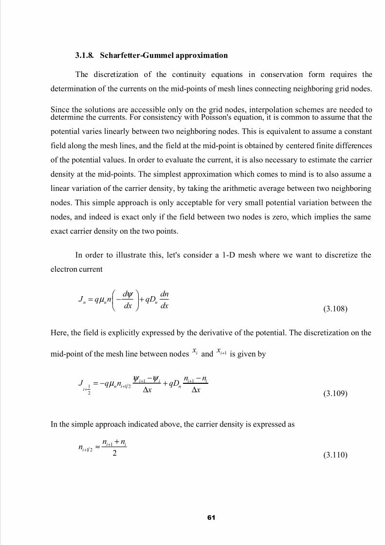
5/13/2018 eBook.comp Electronics - slidepdf.com
http://slidepdf.com/reader/full/ebookcomp-electronics 61/236
3.1.8. Scharfetter-Gummel approximation
The discretization of the continuity equations in conservation form requires the
determination of the currents on the mid-points of mesh lines connecting neighboring grid nodes.
Since the solutions are accessible only on the grid nodes, interpolation schemes are needed todetermine the currents. For consistency with Poisson's equation, it is common to assume that the
potential varies linearly between two neighboring nodes. This is equivalent to assume a constant
field along the mesh lines, and the field at the mid-point is obtained by centered finite differences
of the potential values. In order to evaluate the current, it is also necessary to estimate the carrier
density at the mid-points. The simplest approximation which comes to mind is to also assume a
linear variation of the carrier density, by taking the arithmetic average between two neighboring
nodes. This simple approach is only acceptable for very small potential variation between the
nodes, and indeed is exact only if the field between two nodes is zero, which implies the same
exact carrier density on the two points.
In order to illustrate this, let's consider a 1-D mesh where we want to discretize the
electron current
n n n
d dn J q n qD
dx dx
ψ µ
= − + (3.108)
Here, the field is explicitly expressed by the derivative of the potential. The discretization on the
mid-point of the mesh line between nodes i x and 1i x + is given by
1 11 1 2
2
i i i in i n
i
n n J q n qD
x x
ψ ψ µ + +
++
− −= − +
∆ ∆ (3.109)
In the simple approach indicated above, the carrier density is expressed as
11 2 2
i ii
n nn +
+
+≈
(3.110)
61

5/13/2018 eBook.comp Electronics - slidepdf.com
http://slidepdf.com/reader/full/ebookcomp-electronics 62/236
In Eq. (3.90), the assumed linearity of the potential between meshes, is implied by the use of the
centered finite differences to express the field on the mid-point. We can now rewrite Eq. (3.90)
including the approximation in Eq. (3.91) as
1 11 1
22 2
n i i n n i i ni i
i
ba
D D J n q q n q q
x x x x
µ ψ ψ µ ψ ψ + ++
+
− − = − + − + ∆ ∆ ∆ ∆
1 442 4 43(3.111)
If we assume a condition where 0n J = (equilibrium) and a >> b (negligible diffusion), it is easy
to see that positivity of the carrier density is not guaranteed, since the solution oscillates as
1i in n+ ≈ − . Also, it can be shown that for stability we need to have 1 2 /i i Bk T qψ ψ + − > , which
requires very small mesh spacing to be verified.
The approach by Scharfetter and Gummel [51] has provided an optimal solution to this
problem, although the mathematical properties of the proposed scheme have been fully
recognized much later. We consider again a linear potential variation between neighboring mesh
points, which is consistent with the use of finite differences to express the field. We express the
current in the interval [ ]1;i i x x + as a truncated expansion about the value at the mid-point
1 1
2 2
( ) ( ) ( )n n ni i
J x J x x x J x x
δ
δ + +
= + −
(3.112)
From Eq. (3.93) we obtain a first order differential equation for n J which can be solved to
provide n( x) in the mesh interval, using as boundary conditions the values of carrier density in
and 1in + . We obtain
[ ] 1( ) 1 ( , ) ( , ) ;i in x g x n g x nψ ψ += − + [ ]1;i i x x x +∈
(3.113)
where ( , ) g x ψ is the growth function
62
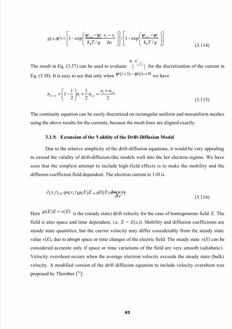
5/13/2018 eBook.comp Electronics - slidepdf.com
http://slidepdf.com/reader/full/ebookcomp-electronics 63/236
1 1( , ) 1 exp / 1 exp/ /
i i i i i i
B B
x x g x
k T q x k T q
ψ ψ ψ ψ ψ + +
− − −= − − ∆ (3.114)
The result in Eq. (3.57) can be used to evaluate ( )1 2in x
+ for the discretization of the current in
Eq. (3.58). It is easy to see that only when ( 1) ( ) 0i iψ ψ + − = we have
11/ 2 1
1 11
2 2 2i i
i i i
n nn n n +
+ +
+ = − + = (3.115)
The continuity equation can be easily discretized on rectangular uniform and nonuniform meshes
using the above results for the currents, because the mesh lines are aligned exactly.
3.1.9. Extension of the Validity of the Drift-Diffusion Model
Due to the relative simplicity of the drift-diffusion equations, it would be very appealing
to extend the validity of drift-diffusion-like models well into the hot electron regime. We have
seen that the simplest attempt to include high-field effects is to make the mobility and the
diffusion coefficient field dependent. The electron current in 1-D is
( , )( , ) ( , ) ( ) ( ) n x t J x t qn x t E E qD E x
δ µ δ
= +(3.116)
Here ( ) ( ) E E v E µ = is the (steady state) drift velocity for the case of homogeneous field E . The
field is also space and time dependent, i.e. E = E ( x,t ). Mobility and diffusion coefficients are
steady state quantities, but the carrier velocity may differ considerably from the steady state
value v( E ), due to abrupt space or time changes of the electric field. The steady state v( E ) can be
considered accurate only if space or time variations of the field are very smooth (adiabatic).
Velocity overshoot occurs when the average electron velocity exceeds the steady state (bulk)
velocity. A modified version of the drift diffusion equation to include velocity overshoot was
proposed by Thornber [52]:
63

5/13/2018 eBook.comp Electronics - slidepdf.com
http://slidepdf.com/reader/full/ebookcomp-electronics 64/236
( , ) ( , )( , ) ( , ) ( ) ( ) ( ) ( ) ( )
E E n x t n x t J x t qn x t v E W E B E qD E qA E
x t x t
δ δ δ δ
δ δ δ δ
= + + + + (3.117)
where three new terms have been added. The term with W ( E ) contains the field gradient and
corrects the local drift velocity for spatial velocity overshoot effects. The term with B( E )
contains the time derivative of the field and corrects for time-dependent velocity overshoot. The
last term with A( E ) preserves the invariances of the total current (note that this term does not
represent generation, recombination, trapping, etc., effects which may be incorporated with an
additional term). The quantities W ( E ), B( E ), and A( E ) must be tabulated from detailed transport
calculations. In steady state the current equation simply becomes
( ) ( ) ( ) ( ) ( ) E n
J x qn x v E W E qD E x x
δ δ
δ δ = + + (3.118)
and the resulting continuity equation is
( )( ) ( ) ( ) ( ) ( )
n x E nn x v E n x W E D E
x x x x
δ δ δ δ
δ δ δ δ
= + + (3.119)
Eq. (3.63) does not describe a real transient, since the time derivatives in the current equation
have been neglected. Therefore Eq. (3.63) is valid in the steady state limit0
n
t
δ
δ =
, i.e. t → ∞ .
The equation may be used, however, to solve the pseudo-time-dependent problem until steady
state is achieved. Since the Poisson equation is solved at each time step, the fields and the related
variable are continuously updated in space. Alternatively, one may solve the steady-state
equation obtained with
0n
t
δ
δ
=
, using Newton's method, for instance. Developing the spacederivatives, Eq. (3.63) becomes [53]
64

5/13/2018 eBook.comp Electronics - slidepdf.com
http://slidepdf.com/reader/full/ebookcomp-electronics 65/236
2
2
2
2
( )( ) ( ) ( ) ( ) ( ) ( )
( ) ( )( ) ( ) ( ) ( ) ( )
x
n n v E n E nv E n x W E E n x W E D E
t x x x x x x
v E E E D E nW E n x v E W E D E
x x x x x x x
δ δ δ δ δ δ
δ δ δ δ δ δ
δ δ δ δ δ δ
δ δ δ δ δ δ
∂ = + + + + ∂ = + + + + ∂ (3.120)
Finally, the pseudo-time-dependent equation has form
2
2( , ) ( , ) ( , )
n n na x t b x t c x t n
t x x
δ
δ
∂ ∂= + +
∂ ∂ (3.121)
Since from Gauss law
E
x
δ ρ ε
δ =
and ρ depends on the carrier density n( x), the coefficients
b( x,t ) and c( x,t ) are also functions of n( x) and Eq. (3.102) is nonlinear. Often the overshoot
parameter W ( E ) is rewritten in terms of mobility, as ( ) ( ) ( )W E E L E µ = , where L( E ) is called
length coefficient. Monte Carlo calculations as well as analytical models for the length
coefficient have been presented in the literature. Extension to 2-D is not trivial when confining
fields (barriers) besides accelerating fields are present. An approximate approach allows the
extension to 2-D by using the gradient of the quasi-Fermi levels (very flat inside barrier regions
but following the potential profile in accelerating regions) as the functional parameter for the
length coefficient [54].
Problems
1. Plot the doping dependence of the low-field electron mobility, as described by the
conventional mobility model, Klaassen's mobility model, the Arora model and the Dorkel
and Leturg model. In your calculation use the parameters specified in the Silvaco
ATLAS manual or the corresponding paper. Consider n-type semiconductor with donor
doping density varying from 1014 cm-3 to 1020 cm-3.
2. Assume that the doping density is N D=1017 cm-3. Plot the field-dependent mobility using
each of the above-described low-field mobility models and the expressions for the field-
dependent mobility and saturation velocity. Vary the electric field value between 0.1
65

5/13/2018 eBook.comp Electronics - slidepdf.com
http://slidepdf.com/reader/full/ebookcomp-electronics 66/236
kV/cm and 100 kV/cm. Compare your results with those obtained with the Scharfetter
and Gummel model, described by expressions 4.1-50 and 4.1-23 in Selberherr's book.
3. Derive the expression for the SRH generation/recombination rate presented in class.
What are the limiting values to this expression under low and high injection conditions
and when and where do they occur?
4. Plot the perpendicular field dependence of the low-field electron mobility using the
Yamaguchi and the Shirahata models. In your calculations assume n-channel MOSFET
device with uniform substrate doping equal to 3.9× 1015 cm-3, 2× 1016 cm-3, 7.2× 1016 cm-3
and 3× 1017 cm-3. Vary the transverse electric field from 104 V/cm to 106 V/cm. Compare
your model results with the experimental data of Takagi, Toriumi, Iwase and Tango
(IEEE Trans. Electron Devices, Vol. 41, pp. 2357-2362, 1994).
5. To obtain diagonaly-dominant coefficient matrix when using finite difference scheme for
the discretization of the Poisson equation, it is necessary to use some linearization
scheme. The simplest way to achieve this is to use δ+ψ →ψ , where δ is small.
(a) Write down (derive) the linearized Poisson equation using this linearization
scheme.
(b) Write down (derive) the scaled version of the result obtained in (a).
(c) Write the finite-difference approximation for the scaled Poisson equation. If one
solves (c) for the improvement δ , show that the resultant coefficient matrix A is
diagonally dominant. (Note: Matrix A is diagonally dominant if the absolute value
of the sum of the off-diagonal elements in each row is smaller than the absolute
value of the corresponding diagonal term.)
6. Consider a 1D sample, such that for b x x
< the semiconductor has a dielectric constant 1ε
, and for b x x > has dielectric constant 2ε . At the interface between the two
semiconductor materials ( b x x = ), there are no interface charges. Starting from the
condition
66

5/13/2018 eBook.comp Electronics - slidepdf.com
http://slidepdf.com/reader/full/ebookcomp-electronics 67/236
bb x x x x x x == ∂ψ ∂
ε=∂ψ ∂
ε 21
and using Taylor series expansion for ψ around b x x = (for b x x < and b x x > ), calculate
the finite difference approximation of the Poisson equation at b x x = .
7. This example is a demonstration of the fact that explicit numerical integration methods
are incapable of solving even the problem of linearly-graded junctions in thermal
equilibrium, for which mx N N A D =− , where a is the edge of the depletion region. To
demonstrate this, calculate the following:
• Establish the boundary conditions for the electrostatic potential [ )( a−ψ and )(aψ ]
by taking into account the free carrier terms in the equilibrium 1D Poisson equation:
( ) ( )mxenene
mxn pe
x
V i
V
it +−
ε−=+−
ε−=
∂
ψ ∂ ψ ψ − //
2
2
• Solve analytically the 1D Poisson equation for )( xψ within the depletion
approximation (no free carriers) and calculate a using this result as well as the boundaryconditions found in (a). What is the expression for absolute value of the maximum
electric field.
• Apply the explicit integration method for the numerical solution of the 1D
Poisson equation (that includes the free carriers) by following the steps outlined below:
o Write a Taylor series expansion for )( xψ around x=0, keeping the terms up to the
fifth order.
o Starting from the equilibrium Poisson equation, analytically calculate )0("ψ ,
)0()3(ψ , )0()4(ψ and )0()5(ψ .
o Use the maximum value of the electric field derived in (b) to determine from the
Taylor series expansion for )( xψ , the terms )(hψ , )2( hψ and )3( hψ .
67

5/13/2018 eBook.comp Electronics - slidepdf.com
http://slidepdf.com/reader/full/ebookcomp-electronics 68/236
o Compute )( xψ at x=4h, 5h, 6h, … , up to m x µ= 5.0max , using the predictor-
corrector method in which the predictor formula:
ψ +ψ −ψ +ψ +ψ −ψ =ψ −−−−−+ 3
242
"
2
"
1
"
" 12311 iiiiiii h
o is applied to predict 1+ψ i , which is then corrected by the corrector formula:
ψ +ψ −ψ +ψ +ψ −ψ =ψ −+
−+ 12
22
"1
""1"2
11iii
iiii h
.
o In both, the predictor and the corrector formulas, the second derivatives are
obtained from the Poisson's equation. The role of the predictor is to provide"
1+ψ i
that appears in the corrector formula.
• Repeat the above procedure for the following values of the first derivative:
o Trial 1: )0(')0(' 1 ψ =ψ ,
o Trial 2: 2/)0(')0(' 12 ψ =ψ ,
o Trial 3: [ ]213 )0(')0('5.0)0(' ψ +ψ =ψ .
o Repeat the above described process for several iteration numbers, say up to n=22.
Comment on the behavior of this explicit integration scheme.
Use the following parameters in the numerical integration:
.102,10,104.1
,300,/10064.112,10602.17421310
120
19
cmhcmmcmn
K T cm F C e
i
−−−
−−
×==×=
=×=ε=ε×=
8. Write a 1D Poisson equation solver that solves the linearized Poisson equation for a pn-
junction under equilibrium condition, with:
(a)315315 10,10 −− == cm N cm N D A ,
68

5/13/2018 eBook.comp Electronics - slidepdf.com
http://slidepdf.com/reader/full/ebookcomp-electronics 69/236
(b)316316 10,10 −− == cm N cm N D A ,
(c)318316 10,10 −− == cm N cm N D A .
For each of these three device structures:
- Calculate analytically the maximum allowed mesh size in each region.
- Plot the conduction band edge versus distance assuming that the Fermi level is
the reference energy level ( 0= F E ).
- Plot the total charge density versus distance.
- Plot the electric field versus distance. Calculate the electric field using centered
difference scheme.
- Plot electron and hole densities versus distance.
- Calculate analytically, using the block-charge approximation, the width of the
depletion regions and the magnitude of the peak electric field, and compare the
analytical with the numerical simulation results. When is the block-charge
approximation invalid?
9. Develop a one-dimensional (1D) drift-diffusion simulator for modeling pn-junctions
(diodes) under forward and reverse bias conditions. Include both types of carriers in your
model (electrons and holes). Derive the finite-difference expressions for the electron and
hole current continuity equations using Sharfetter-Gummel discretization scheme, which
was described in the class. Compare your final answers with the expressions given inSelberherr's book.
Model:
69

5/13/2018 eBook.comp Electronics - slidepdf.com
http://slidepdf.com/reader/full/ebookcomp-electronics 70/236
Silicon diode, with permittivity F/m1005.1 10−×=ε sc and intrinsic carrier
concentration310 cm105.1 −×=in at T=300K. In all your simulations assume that
T=300K. Use concentration-dependent and field-dependent mobility models and SRH
generation-recombination process. Assume ohmic contacts and charge neutrality at
both ends to get the appropriate boundary conditions for the potential and the electron
and hole concentrations.
For the concentration-dependent electron and hole mobilities use the Arora model
given in the Silvaco Manuals. It will be easier, while you are developing the 1D
simulator, to assume constant mobility (concentration and field-independent) model.
For the field-dependent mobility, use the model described in the class notes and in the
Silvaco ATLAS manual, using the relevant parameters listed there.
For the SRH generation-recombination, use the expressions given in the text. To
simplify your calculations, assume that the trap energy level coincides with the
intrinsic level.
Doping: Use N cm
A =
−1016 3 and
N cmD =
−1017 3 as a net doping of the p- and n-
regions, respectively.
Poisson solver:
Modify your solver that you developed in Problem #8 to solve the linear Poisson
equation:
[ ])()(2
2
x N x N n pe x
A D sc
−+−ε−=∂ ψ ∂
Numerical methods: Use the LU decomposition method for the solution of the 1D
Poisson and the two 1D continuity equations for electrons and holes individually. Use
70

5/13/2018 eBook.comp Electronics - slidepdf.com
http://slidepdf.com/reader/full/ebookcomp-electronics 71/236
Gummel's decoupled scheme, described in the class and in the distributed notes, to
solve the resultant set of coupled set of algebraic equations.
Outputs:
Plot the conduction band edge under equilibrium conditions (no current flow).
Vary the Anode bias VA from 0 to 0.6 V, in voltage increments that are fraction of
the thermal voltage V k T qT B= / , to have stable convergence. Plot the resulting IV
characteristics. The current will be in A/unit area, since you are doing 1D modeling.
Check the conservation of current when going from the cathode to the anode, which
also means conservation of particles in your system. For the calculation of the currentdensity, use the results given in the notes.
For VA =0.5 V, plot the position of the electron and hole quasi-Fermi levels, with
respect to the equilibrium Fermi level, assumed to be the reverence energy level.
Final note: When you submit your project report, in addition to the final results, give
a brief explanation of the problem you are solving with reference to the listing of your
program that you need to turn in with the report.
4. Hydrodynamic Model
The current drive capability of deeply scaled MOSFETs and, in particular, n-MOSFETs has been
the subject of investigation since the late 1970s. First it was hypothesized that the effective
carrier injection velocity from the source into the channel would reach the limit of the saturation
velocity and remain there as longitudinal electric fields increased beyond the onset value for velocity saturation. However, theoretical work indicated that velocity overshoot can occur even
in silicon [55], and indeed it is routinely seen in the high-field region near the drain in simulated
devices using energy balance models or Monte Carlo. While it was understood that velocity
overshoot near the drain would not help current drive, experimental work [ 56,57] claimed to
71

5/13/2018 eBook.comp Electronics - slidepdf.com
http://slidepdf.com/reader/full/ebookcomp-electronics 72/236
observe velocity overshoot near the source, which of course would be beneficial and would make
the drift-diffusion model invalid.
In the computational electronics community, the necessity for the hydrodynamic (HD)
transport model is normally checked by comparison of simulation results for HD and DD
simulations. Despite the obvious fact that, depending on the equation set, different principal
physical effects are taken into account, the influence on the models for the physical parameters is
more subtle. The main reason for this is that in the case of the HD model, information about
average carrier energy is available in form of carrier temperature. Many parameters depend on
this average carrier energy, e.g., the mobilities and the energy relaxation times. In the case of the
DD model, the carrier temperatures are assumed to be in equilibrium with the lattice temperature,
that is C LT T = , hence, all energy dependent parameters have to be modeled in a different way.
4.1.Extensions of the Drift-Diffusion model
The DD model is the simplest current transport model which can be derived from
Boltzmann’s transport equation (BTE) by the method of moments [58] or from basic principles of
irreversible thermodynamics [59]. For many decades, the DD model has been the backbone of
semiconductor device simulation. In this model, the electron current density is
phenomenologically expressed as consisting of two components. The drift component is driven
by the electric field and the diffusion component by the electron density gradient. It is given by
( )J En nq n D n µ = + ∇ (4.122)
where µ and n D are the mobility and the diffusivity of the electron gas, respectively, and are
related to each other by the Einstein relation for non-degenerate semiconductors
B nn
k T D
q µ = (4.15)
where Bk is the Boltzmann constant. The current relation Eq. (4.1) is inserted into the continuity
equationJ t q n∇ ⋅ = ∂ (4.123)
to give a second-order parabolic differential equation, which is then solved together with
Poisson’s equation. Note that generation/recombination effects were neglected in Eq. (4.3).
72

5/13/2018 eBook.comp Electronics - slidepdf.com
http://slidepdf.com/reader/full/ebookcomp-electronics 73/236
In the DD approach, the electron gas is assumed to be in thermal equilibrium with the
lattice temperature ( )n LT T = . However, in the presence of a strong electric field, electrons gain
energy from the field and the temperature nT of the electron gas is elevated. Since the pressure of
the electron gas is proportional to B nnk T , the driving force now becomes the pressure gradient
rather then merely the density gradient. This introduces an additional driving force, namely, the
temperature gradient besides the electric field and the density gradient. Phenomenologically, one
can write
( )J En n T nq n D n nD T µ = + ∇ + ∇ (4.124)
where T D is the thermal diffusivity.
Although the DD equations are based on the assumption that the electron gas is in
thermal equilibrium with the lattice, an estimation for the local temperature can be calculated
with the local energy balance equation [60]
2
221
3n L L
B c
q E T T E T
k E ε τ µ
= + = +
(4.125)
where ε τ is the energy relaxation time. Eq. (4.5) is obtained under the assumption of a local
energy balance. At the critical electric field E c, which depends on the electric field via the
mobility, the carrier temperature reaches twice the value of the lattice temperature. c E is in the
order of 10 kV/cm, a value easily exceeded even in not very advanced devices where values
higher than 1 MV/cm can be observed [61]. Note too that the temperature obtained from Eq. (4.4)
introduces an inconsistency with the assumptions made during the derivation of the DD model
where the electron gas has been assumed to be in equilibrium with the lattice temperature.
For a rapidly increasing electric field, however, the average energy lags behind the
electric field, and the assumption of local equilibrium becomes invalid [62]. A consequence of the
lag is that the maximum energy can be considerably smaller than the one predicted by the localenergy balance equation. An important consequence of this behavior is that the lag of the average
energy gives rise to an overshoot in the carrier velocity. The reason for the velocity overshoot is
that the mobility depends to first order on the average energy and not on the electric field. As the
mobility has not yet been reduced by the increased energy but the electric field is already large,
73

5/13/2018 eBook.comp Electronics - slidepdf.com
http://slidepdf.com/reader/full/ebookcomp-electronics 74/236
an overshoot in the velocity is observed until the carrier energy comes into equilibrium with the
electric field again.
Similar to the carrier mobility, many other physical processes like impact ionization are
more accurately described by a local energy model rather than a local electric field model,
because these processes depend on the distribution function rather than on the electric field.
Altogether, it can be noted that modeling of deep-submicrometer devices with the DD model is
becoming more and more problematic. Although successful reproduction of terminal
characteristics of nanoscale MOS transistors has been reported with the DD model [63], the
values of the physical parameters used significantly violate basic physical principles. In
particular, the saturation velocity had to be set to more than twice the value observed in bulk
measurements. This implies that the model is no longer capable of reproducing the results of
bulk measurements and as such looses its consistency. Furthermore, the model can hardly be
used for predictive simulations. These solutions may provide short-term fixes to available
models, but obtaining “correct” results from the wrong physics is unsatisfactory in the long run.
In the following, we first give a brief description of the Straton’s approach, which has
been one of the first attempts to address all of the above issues. Then, we present the derivation
and discuss the properties of the hydrodynamic model and its simplifications from the moments
of the Boltzmann’s transport equation introduced in Chapter 2 of this book.
4.2.Stratton’s Approach
One of the first derivations of extended transport equations was performed by Stratton
[64]. First the distribution function is split into the even and odd parts
0 1( , ) ( , ) ( , )k r k r k r f f f = + . (4.126)
From 1 1( , ) ( , )k r k r f f − = − , it follows that 1 0 f = . Assuming that the collision operator C is
linear and invoking the microscopic relaxation time approximation for the collision operator
[ ] ( , )r
eq f f
C f τ ε
−
= − (4.127)
the BTE can be split into two coupled equations. In particular f 1 is related to f 0 via
( )1 0 0, r k r v Eq
f f f τ ε = − ⋅∇ − ⋅∇ h
. (4.128)
The microscopic relaxation time is then expressed by a power law
74

5/13/2018 eBook.comp Electronics - slidepdf.com
http://slidepdf.com/reader/full/ebookcomp-electronics 75/236
0( )
p
B Lk T
ε τ ε τ
−
=
. (4.129)
When f 0 is assumed to be heated Maxwellian distribution, the following equation system is
obtained
Jn
qt
∂∇ ⋅ =
∂
( )J E B nqn k n T µ µ = + ∇
( ) ( )3 3
2 2S E J n L
B n B
T T n k nT k n
ε τ
−∇ ⋅ = − ∂ + ⋅ −
( )25
2S E+ B
B n n
k n p nk T n T
q µ µ
= − − ∇
(4.130)
Eq. (4.4) for the current density can be rewritten as:
( )1 B Bn n n
k k J q nE T n n T
q q µ ν
= + ∇ + + ∇
(4.131)
with
ln
ln
nn
n n
T
T T
µ µ ν
µ
∂ ∂= =
∂ ∂ (4.132)
which is commonly used as a fit parameter with values in the range [-0.5,-1.0]. For nν =-1.0, the
thermal distribution term disappears. The problem with Eq. (4.9) for τ is that p must be
approximated by an average value to cover the relevant processes. In the particular case of
impurity scattering, p can be in the range [-1.5,0.5], depending on charge screening. Therefore,
this average depends on the doping profile and the applied field; thus, no unique value for p can
be given. Note also that the temperature T n is a parameter of the heated Maxwellian distribution,
which has been assumed in the derivation. Only for parabolic bands and a Maxwellian
distribution, this parameter is equivalent to the normalized second-order moment.
4.3.Balance Equations Model
In this section, we will first describe the prescription for generating the balance equations from
the BTE, which in its most general form is given by
( ) ( , , )k E r pr op
f evf f S f s t
t
∂+ ∇ ⋅ − ⋅∇ = +
∂ h(4.133)
75

5/13/2018 eBook.comp Electronics - slidepdf.com
http://slidepdf.com/reader/full/ebookcomp-electronics 76/236
We define a quantity ( )pφ , that can have values 1, ,p K , etc., and the total value (averaged) of
the quantity associated with ( )pφ is
1( , ) ( ) ( , , )
p
r p r pn t f t V
φ φ = ∑ (4.134)
where nφ can represent carrier density, current density, etc. To find the balance equation for nφ ,
we need to multiply the BTE by ( ) /p V φ and to integrate over p. Then, the various terms that
appear in the BTE become
( )
1 1( ) ( ) ( , , )
1 1( ) ( ) ( , , )
p p
r r r
p p
p p r p
p v v p r p
n f f t
V t t V t
f f t F V V
φ
φ
φ φ
φ φ
∂ ∂ ∂= = ∂ ∂ ∂
∇ ⋅ = ∇ ⋅ = ∇ ⋅
∑ ∑
∑ ∑(4.135)
where1
( ) ( , , )p
v p r p F f t V
φ φ = ∑ is the flux associated with nφ . For example, if ( ) 1pφ = , then F φ
is the carrier flux, and if ( )p p E φ = , then F φ is the energy flux. The third term is then given by
( ) ( )
( , , ) ( )
p p
p p
p
p
p E E p
E r p p
e f e f
e f t Gφ
φ φ
φ
− ⋅∇ = − ⋅ ∇
= ⋅ ∇ = −
∑ ∑
∑(4.136)
and is called a generation term since electric field increases momentum and the quantity nφ .
There is another term ( , , )r p s t that leads to increase/decrease of nφ (generation-recombination
process). The contribution of these terms is
1( , ) ( ) ( , , )
p
r p r pS t s t V
φ φ = ∑ (4.137)
The collision events, for example, destroy momentum and thus represent a recombination term
01 1
( ) ( , ) ( , )pp r r
coll
f
R n t n t V t φ φ φ φ
φ τ
∂ = − = − ∂∑ (4.138)
where 1 φ τ is the ensemble relaxation rate. To find the definition of this term we assume
non-degenerate semiconductor, for which
76

5/13/2018 eBook.comp Electronics - slidepdf.com
http://slidepdf.com/reader/full/ebookcomp-electronics 77/236
[ ]'
( , ', ) ( ', ) ( , , ) ( , ')r p p p r p p p pcoll
f f t S f t s
t
∂= −
∂ ∑ (4.139)
Then:
'
1 1 ( ')( ) ( ) ( , , ) 1 ( , ')( )
1 1( ) ( , , )
( )
p p p
p
pp p r p p p
p
p r pp
coll
f f t S V t V
f t V φ
φ φ φ φ
φ τ
∂ = − − ∂
= −
∑ ∑ ∑∑
(4.140)
where 1 ( )pφ τ is the total out-scattering rate associated with quantity φ . With little manipulation
of the above expressions, we get
0
1 ( , , ) ( )
( )1
( , ) ( , )
p
r p p
p
r r
f t
V
n t n t
φ
φ φ φ
φ
τ
τ =
−
∑. (4.141)
This ensemble relaxation rate depends upon the type of the scattering mechanism and how
carriers are distributed in momentum. In summary, when ( )p i pφ = , then in P φ = and
1ii
coll m
dP P
dt τ = − . (4.142)
Also, when ( ) ( )p p E φ = , then n W φ = (average kinetic energy density) that is given by W nu=
(u equals the average energy density per electron). Then
( )0
1
coll E
dW W W
dt τ = − − . (4.143)
Note that the results presented up to this point are exact, i.e. no relaxation time approximation
discussed in Chapter 3 is made. By summarizing all of the above results, we arrive at the balance
equation for the quantity nφ , of the form
n F G R S
t
φ
φ φ φ φ
∂= −∇ ⋅ + − +
∂. (4.144)
Carrier-density balance equation
When ( ) 1pφ = , then n nφ = (electron density),1 1
( , , ) ( , )p
F v r p J rn f t t V e
φ = = −∑ ,
0G Rφ φ = = (scattering mechanisms and the electric field redistribute carriers among states but
77

5/13/2018 eBook.comp Electronics - slidepdf.com
http://slidepdf.com/reader/full/ebookcomp-electronics 78/236
do not generate or destroy carriers). The above results lead to the continuity equation for the
electrons, which is nothing more but a conservation of particle in the system
1Jn n
nS
t e
∂= ∇ ⋅ +
∂. (4.145)
The momentum balance equation
The momentum balance equation is obtained by assuming ( )p z pφ = , for example. Then, the
various quantities that appear in the balance equation are of the following form
1( , , )
1 1( , , ) *
p
p p
r p
F v r p
z z
z i z i
n p f t P V
p f t F m v v f V V
φ
φ φ
= =
= → =
∑
∑ ∑(4.146)
In the above expressions P z is the total momentum density along z , and 2i iz F W φ = , where iz W is a
component of the kinetic energy density tensor. The generation and the recombination term
reduce to
( , , )p
p
E r p z z G e f t p eE nφ = − ⋅ ∇ = −∑ (4.147)
1 z
m
R P φ τ
= (4.148)
Then, the momentum balance equation for P z reads1 1
2 iz z z z z
im i m
W P F enE P enE P
t xφ
τ τ
∂∂= −∇ ⋅ − − = − − −
∂ ∂∑ (4.149)
The trace of the tensor for the total energy density W is
( ) 2 21 1 1* ( , , ) *
2 2ii i i
i i p p i
Tr W W m v f f r p t m v W nuV V
= = = = =∑ ∑ ∑ ∑ ∑t
(4.150)
For simple parabolic bands, we have * * /P v Jd nm m e= = − , which gives / *J Pe m= − or
22 1* *
iz z z z
i i m
W J e ne E J
t m x m τ ∂∂ = + −
∂ ∂∑ . (4.151)
With appropriate simplifications, the balance equation for the current density reduces to the drift-
diffusion equation as discussed later in this section.
Energy Balance Equation
78

5/13/2018 eBook.comp Electronics - slidepdf.com
http://slidepdf.com/reader/full/ebookcomp-electronics 79/236
The energy balance equation is obtained from the prescription that ( )p p E φ = . Then, the
expression for the total energy density is found from
1( ) ( , , )
p
p r pn E f t W V
φ = =∑ , (4.152)
and the energy flux is given by
1( ) ( , , )
p
v p r p FW F E f t V
φ = =∑ (4.153)
The generation and recombination terms that appear in the balance equation are
( , , )E v E Jn
p
eG f r p t
V φ
= ⋅ − = ⋅
∑ , (4.154)
( )0
1
E R W W φ
τ = − (4.155)
where the generation term describes the energy increase due to the electric field and the
recombination term gives the loss of energy due to phonons. The final form of the energy
balance equation, which is nothing more but a statement for the conservation of energy in the
system, is
( )0
1F E JW
E
W W W
t τ
∂= −∇⋅ + ⋅ − −
∂. (4.156)
The term on the LHS, which describes an increase in energy is balanced by the terms on the
RHS. The first term on the RHS describes the energy flowing into the volume, the second one
gives the energy increase due to field accelerating the carriers and the last term desribes the
energy loss due to collisions.
Complete Hydrodynamic Equations
In summary, the first three balance equations take the form
( )
2
0
1
2 1
* *
1
J
F E J
n n
iz z z z
i i m
W
E
nS
t e
W J e ne E J
t m x m
W W W
t
τ
τ
∂= ∇ ⋅ +
∂∂∂
= + −∂ ∂
∂= −∇⋅ + ⋅ − −
∂
∑ (4.157)
79

5/13/2018 eBook.comp Electronics - slidepdf.com
http://slidepdf.com/reader/full/ebookcomp-electronics 80/236
The balance equation for the carrier density introduces the carrier current density, which balance
equation introduces the kinetic energy density. The balance equation for the kinetic energy
density, on the other hand, introduces the energy flux. Therefore, a new variable appears in the
hierarchy of balance equations and the set of infinite balance equations is actually the solution of
the BTE.
The balance equations can be reformulated in a more convenient way by separating the
carrier temperature T C from the lattice temperature T L. To achieve this, we will work on the
kinetic energy density tensor and write the carrier velocity as v v cd = + , where the first term
describes the average drift velocity and the second term describes the random thermal
component. Then, ( ) ( )i z di i dz z di dz i dz z di i z v v v c v c v v c v c v c c= + + = + + + , where the brackets
<> represent an average over the distribution function. Now, since 0ic = , we have
i z di dz i z v v v v c c= + . The kinetic energy tensor component iz
W is, thus, given by
1 1 1* * *
2 2 2iz i z di dz i z W nm v v nm v v nm c c= = + (4.158)
where the first term on the right represents the drift energy iz K and the second term describes the
thermal energy due to the random thermal motion of the carriers. The kinetic energy density
equals the trace of the tensor W , i.e.2 2
, ,
2 2
1 1* *
2 2
1 1* *
2 2
ii di i
i x y z i i
d
W W nm v nm c
nm v nm c
=
= = +
= +
∑ ∑ ∑(4.159)
For the thermal carrier energy we have
2 2 21 1 3 3* * *
2 2 2 2i B C i
i
nm c nm c nk T nm c= = =∑ (4.160)
Therefore21 1
*2 2i B C nm c nk T = ,
* B
i j ij
k c c T
m= (4.161)
and
1 1 1 1* * * *
2 2 2 2 * B
iz di dz i z di dz iz
k W nm v v nm c c nm v v nm T
m= + = + (4.162)
80

5/13/2018 eBook.comp Electronics - slidepdf.com
http://slidepdf.com/reader/full/ebookcomp-electronics 81/236
where iz T is a component of the temperature tensor.
We now want to express the energy flux in terms of the temperature tensor. The energy
flux, defined earlier and repeated here for convenience, is calculated using
1 ( ) ( , , )p
F v p r pW E f t V = ∑ , (4.163)
which means that the i-th component of this vector equals to
( )
22
2 2 2
1 * *( , , )
2 2
*2
2
p
r pWi i i
di dj j dj i j i j
j j j
di B ij dj i
j
m v nm F v f t v v
V
nmv v c v c c c c
v W nk T v Q
= =
= + + +
= + +
∑
∑ ∑ ∑
∑
(4.164)
where iQ is the component of the heat flux vector which describes loss of energy due to flow of
heat out of the volume. To summarize, the kinetic energy flux equals the sum of the kinetic
energy density times velocity plus the velocity times the pressure, which actually represents the
work to push the volume plus the loss of energy due to flow of heat out. In mathematical terms
this is expressed as
F v v QW BW nk T = + ⋅ + . (4.165)
With the above considerations, the momentum and the energy balance equations reduce to
( ) ( )
2
0
2 1 1
* 2 *
1v Q v E J
z iz B iz z z
i i m
B n
E
J e ne K nk T E J
t m x m
W W nk T W W
t
τ
τ
∂ ∂ = + + − ∂ ∂
∂= −∇⋅ + + ⋅ + ⋅ − −
∂
∑
t(4.166)
4.3.1. Displaced Maxwellian Approximation
Most common way to solve the balance equations is to guess a form for the distribution
function and use the balance equations to solve for the parameters in this functional form. Most
commonly used form is displaced-Maxwellian
2( ) exp * / 2 *p p vd B c f m m k T ∝ − − (4.167)
81

5/13/2018 eBook.comp Electronics - slidepdf.com
http://slidepdf.com/reader/full/ebookcomp-electronics 82/236
This is a good model for cases when the electron-electron interactions thermalize the distribution
function. For a displaced Maxwellian, the temperature tensor is diagonal, i.e. ij c ijT T δ = . With
these approximations
1 1 1
2 2 2 B c iz B ci i z
nk T nk T x xδ
∂ ∂ = ∂ ∂ ∑ . With this simplifications, the
current density (momentum) balance equation becomes
( )22 1
* * *iz z
B c z z
i i z m
K J e e nenk T E J
t m x m x m τ
∂∂ ∂= + + −
∂ ∂ ∂∑ (4.168)
The momentum balance equation can be immediately obtained by multiplying the above result
by ( )1
/ *e m−− to get
( ) 12 iz z B c z z
i i z m
K P nk T enE P t x x τ
∂∂ ∂= − − − −∂ ∂ ∂∑ (4.169)
Therefore, to solve the balance equation for P z (or equivalently J z ), one needs to know the carrier
temperature. (1) Under low-field conditions, the carrier temperature T c can be assumed to be
equal to the lattice temperature T L. (2) Under high-field conditions, the carrier temperature T c is
larger than the lattice temperature, and under these circumstances one needs to solve the energy
balance equation that is discussed next.
For displaced-Maxwellian approximation for the distribution function, the heat flux Q =0. However, Blotekjaer [65] has pointed out that this term must be significant for non-Maxwellian
distributions, so that a phenomenological description for the heat flux, of the form described by
Franz-Wiedermann law, which states that
Q cT κ = − ∇ (4.170)
is used, where κ is the thermal or heat conductivity. In silicon, the experimental value of κ is
14 W/cmK. The above description for Q actually leads to a closed set of equations in which the
energy balance equation is of the form
( ) ( )0
1v v E Jc B c n
E
W W T nk T W W
t κ
τ
∂= −∇⋅ − ∇ + + ⋅ − −
∂(4.171)
It has been recognized in recent years that this approach is not correct for semiconductors in the
junction regions, where high and unphysical velocity peaks are established by the Franz-
82

5/13/2018 eBook.comp Electronics - slidepdf.com
http://slidepdf.com/reader/full/ebookcomp-electronics 83/236
Wiedemann law. To avoid this problem, Stettler, Alam and Lundstrom [66] have suggested a new
form of closure
( )5
12
Q J B Lc
k T T r
eκ = − ∇ + − (4.172)
where J is the current density and r is a tunable parameter less than unity. Now using
( ) ( ) ( )2 * *
*
iz di dz di dz
i
di dz dz dz
i z
K nm v v nm v v x x x
v vnm v v
x x
∂ ∂ ∂= =
∂ ∂ ∂
∂ ∂= + ∂ ∂
(4.173)
and assuming that the spatial variations are confined along the z-direction, we have
( ) ( )22 *iz dz
z z
K nm v x x
∂ ∂=
∂ ∂
. (4.174)
To summarize, the balance equations for the drifted-Maxwellian distribution function simplify to
( )
( ) ( )
22
0
1
1*
* *
1
n n
z dz B c z z
z m
c B c dz z z
z z E
n J S
t e
J e nenm v nk T E J
t m x m
T W W nk T v J E W W
t x x
τ
κ τ
∂= ∇⋅ +
∂
∂ ∂= + + −
∂ ∂
∂∂ ∂= − + − + − − ∂ ∂ ∂
(4.175)
where
2
*1 3
*2 2
z dz z
dz B c
e J env P
m
W nm v nk T
= − = −
= +(4.176)
4.3.2. Momentum and Energy Relaxation Rates
Having arrived at the final form of the hydrodynamic equations, the next task is to
calculate the momentum and energy relaxation rates, which in this case are ensemble averagedquantities. For that purpose, for simple scattering mechanisms one can utilize the drifted-
Maxwellian form of the distribution function, but for cases where several scattering mechanisms
are important, one must use bulk Monte Carlo simulations to calculate these quantities.
83

5/13/2018 eBook.comp Electronics - slidepdf.com
http://slidepdf.com/reader/full/ebookcomp-electronics 84/236
(A) Using Drifted-Maxwellian form for the Distribution FunctionAssume that the distribution function is of the form
2*
( ) exp2 *
p vp
d
B c
m f
m k T
−= −
(4.177)
where cT is the carrier temperature and v id dz z v= . Expanding the distribution function gives
2
( ) exp 12 *
p z dz S A
B c B c
p v p f f f
m k T k T
= − + = +
. (4.178)
The ensemble averaged momentum relaxation time is then given by
( , , ) / ( )1
( , , )p
p
r p p
r p
z m
m z
f t p
p f t
τ
τ =
∑∑ . (4.179)
For homogeneous systems ( , , ) ( )r p p f t f = (steady-state). Since ( )pmτ is generally even
function of z p , we therefore have contribution from the asymmetric term only, which gives
2
2
( ) / ( )1
( )p
p
pS z m
m z S
f E p
p f E
τ
τ =
∑∑ (4.180)
Now, if θ is the angle between p and the electric field E = E z i z , we have cos z p p θ = . Also, if
we assume parabolic band structure, for which E (p)= p2/2m*, then
3/ 2
3/ 2
1( )
( )1
( )
S
m
m S
E f E dE e
E f E dE
τ
τ =
∫ ∫
(4.181)
For the case when the energy-dependent momentum relaxation rate is of the form
( )0( )S
m B L E E k T τ τ = , we have
0
1 1 (5 / 2 )(5/2)
s
L
m C
T sT τ τ Γ −= Γ
. (4.182)
For low fields, the standard momentum relaxation rate that enters into the expression for the
mobility is given by
0
( 5 / 2)
(5/2)m
sτ τ
Γ +=
Γ (4.183)
84

5/13/2018 eBook.comp Electronics - slidepdf.com
http://slidepdf.com/reader/full/ebookcomp-electronics 85/236
which shows very different behavior from the result given in Eq. (4.62).
Let us consider acoustic phonon scattering for which 1/ 2 s = − , which then gives
1 m C L A T T τ = . Similarly, for acoustic phonon scattering the ensemble averaged energy
relaxation rate is given by 1 / E L L C B T T T τ = . Now, under steady state conditions and for
homogeneous systems, the momentum and energy balance equations become
( )
2
0
1
*
1
z z
m
z z
E
ne E J
m
J E W W
τ
τ
=
= −
(4.184)
which then leads to
2222
13 * 1 1
C z z C L
B L crit m E
T E E eT T
m k T E τ τ
= + → = +
(4.185)
where E crit is some critical electric field.
(B) Using Bulk Monte Carlo SimulationsAn alternative way of deriving the momentum relaxation rate (ensemble averaged) is to
use steady-state Monte Carlo simulation for bulk materials under uniform electric fields. Under
these conditions, the momentum and energy balance balance equations simplify to the
expressions given in Eq. (??), from where e have that
0
1 1, .
* dz z z
m dz E
env E eE
m v W W τ τ = − = −
−(4.186)
Note that the as-calculated momentum and energy relaxation rates are electric field, i.e. energy-
dependent quantities.
4.3.3. Simplifications That Lead to the Drift-Diffusion Model
To arrive at the drift-diffusion model, we first rewrite the momentum balance equation in
the following form
( )21 * **
1 1 1 z
z dz B c z
z m m m
J e m e m J nm v nk T ne E
t xτ τ τ
∂ ∂+ = + +
∂ ∂ (4.187)
Defining the carrier mobility as
85

5/13/2018 eBook.comp Electronics - slidepdf.com
http://slidepdf.com/reader/full/ebookcomp-electronics 86/236
*
1n
m
e m µ
τ = , (4.188)
we first have for acoustic deformation potential scattering:
( )
0
2
*
1n
c L z crit
e m
A T T E E
µ µ = = + (4.189)
which clearly shows that at high fields the mobility decreases with increasing the in-plane
electric field. We now go back to the momentum balance equation, which we rewrite as
( )21*
1 z
z n dz B c n z
z m
J J nm v nk T ne E
t x µ µ
τ
∂ ∂+ = + +
∂ ∂ (4.190)
The first approximation that we make is to assume that the carrier drift energy is much smaller
than the thermal energy. This approximation is valid for low-field conditions and leads to kinetic
energy density of the form
21 3 3 2*
2 2 2 3dz B c B B cW nm v nk T nk T nk T W = + ≈ → = . (4.191)
Under steady-state conditions, the momentum balance equation simplifies to
2 2
3 3 z n n z n z n
z z
W J W ne E ne E
x x µ µ µ µ
∂ ∂ = + = + ∂ ∂ (4.192)
The above expression suggests that diffusion is associated with gradients in the kinetic energy
density. The simplified expression for the current density J z can also be written as
c z n z n B c B n
z z
cn z n n
z
T n J ne E k T nk
x x
T ne E eD eS
x
µ µ µ
µ
∂∂= + +
∂ ∂∂
= + +∂
(4.193)
Where Dn and S n are the diffusion and the Soret coefficient respectively. As a further
simplification to the drift-diffusion equations, we assume that there are no temperature gradients
in the system. Then, the set of equations that one solves using, for example, the Silvaco
simulation software is
1J
J E
n n
n n n
nS
t e
en eD n µ
∂= ∇ ⋅ +
∂= + ∇
(4.194)
86

5/13/2018 eBook.comp Electronics - slidepdf.com
http://slidepdf.com/reader/full/ebookcomp-electronics 87/236
Note that in the above expressions, the diffusion coefficient and the mobility of the carriers are
low-field quantities. To extend the validity of this model for high-field conditions, one usually
employs field-dependent models for the diffusion coefficient and the mobility. A variety of
models have been developed for this purpose and they are summarized in Appendix B.
4.4.Numerical Solution Schemes for the Hydrodynamic Equations
A large class of initial value (time-evolution) PDEs in one space dimension can be cast
into the form of a flux-conservative equation,
( )u F u
t x
∂ ∂= −
∂ ∂(4.195)
where u and F are vectors, and where (in some cases) F may depend not only on u but also on
spatial derivatives of u. The vector F is called the conserved flux. We will consider, in this
section, a prototypical example of the general flux conservative Eq. (4.76), namely the equation
for a scalar u,
u u
vt x
∂ ∂= −
∂ ∂(4.196)
with v a constant. As it happens, we already know analytically that the general solution of this
equation is a wave propagating in the positive x-direction,
( )u f x vt = − (4.197)
where f is an arbitrary function. However, the numerical strategies that we develop will beequally applicable to the more general equations represented by Eq. (177). In some contexts, Eq.
(4.76) is called an advective equation, because the quantity u is transported by a “fluid flow”
with a velocity v. How do we go about finite differencing Eq. (4.76)? The straightforward
approach is to choose equally spaced points along both the t -and x-axes. Thus denote
0
0
, 0,1, ,
0,1, , j
n
x x j x j J
t t n t n N
= + ∆ == + ∆ =
K
K (4.198)
Letn
ju denote ( ),n ju t x . We have several choices for representing the time derivative term. The
obvious way is to set
1
,
( )n n
j j
j n
u uuO t
t t
+ −∂= + ∆
∂ ∆(4.199)
87

5/13/2018 eBook.comp Electronics - slidepdf.com
http://slidepdf.com/reader/full/ebookcomp-electronics 88/236
This is called forward Euler differencing. While forward Euler is only first-order accurate in Δt ,
it has the advantage that one is able to calculate quantities at timestep 1n + in terms of only
quantities known at time-step n. For the space derivative, we can use a second-order
representation still using only quantities known at time-step n:
1 1 2
,
( )2
n n
j j
j n
u uuO x
t x
+ −−∂= + ∆
∂ ∆(4.200)
The resulting finite-difference approximation to Eq. (4.76) is called the FTCS representation
(Forward Time Centered Space),
1
1 1
2
n n n n
j j j ju u u uv
t x
++ − − −
= − ∆ ∆ (4.201)
which can easily be rearranged to be a formula for
1n
j
u +
in terms of the other quantities. TheFTCS scheme is a fine example of an algorithm that is easy to derive, takes little storage, and
executes quickly. Too bad it doesn’t work!
The FTCS representation is an explicit scheme. This means that1n
ju + for each j can be
calculated explicitly from the quantities that are already known. Later we shall meet implicit
schemes, which require us to solve implicit equations coupling the1n
ju +for various j. The FTCS
algorithm is also an example of a single-level scheme, since only values at time level n have to
be stored to find values at time level n+1.
von Neumann Stability Analysis
Unfortunately, Eq. (4.81) is of very limited usefulness. It is an unstable method, which
can be used only (if at all) to study waves for a short fraction of one oscillation period. To find
alternative methods with more general applicability, we must introduce the von Neumann
stability analysis. The von Neumann analysis is local: We imagine that the coefficients of the
difference equations are so slowly varying as to be considered constant in space and time. In that
case, the independent solutions, or eigenmodes, of the difference equations are all of the formn n ikj x
ju eξ ∆= (4.202)
where k is a real spatial wave number (which can have any value) and ( )k ξ ξ = is a complex
number that depends on k . The key fact is that the time dependence of a single eigenmode is
nothing more than successive integer powers of the complex number ξ . Therefore, the
88

5/13/2018 eBook.comp Electronics - slidepdf.com
http://slidepdf.com/reader/full/ebookcomp-electronics 89/236
difference equations are unstable (have exponentially growing modes) if ( ) 1k ξ > for some k .
The number ξ is called the amplification factor at a given wave number k . To find ξ (k ), we
simply substitute Eq. (4.82) back into Eq. (4.81). Dividing by ξ n, we get
( )( ) 1 sinv t k i k x x
ξ ∆= − ∆∆
(4.203)
whose modulus is > 1 for all k ; so the FTCS scheme is unconditionally unstable. If the velocity
v were a function of t and x, then we would writen
jv in Eq. (4.81). In the von Neumann stability
analysis we would still treat v as a constant, the idea being that for v slowly varying the analysis
is local. In fact, even in the case of strictly constant v, the von Neumann analysis does not
rigorously treat the end effects at j = 0 and j = N . More generally, if the equation’s right-hand
side were nonlinear in u, then a von Neumann analysis would linearize by writing u = u0 + δu,expanding to linear order in δu. Assuming that the u0 quantities already satisfy the difference
equation exactly, the analysis would look for an unstable eigenmode of δu. Despite its lack of
rigor, the von Neumann method generally gives valid answers and is much easier to apply than
more careful methods. We accordingly adopt it exclusively. (See, for example, [67] for a
discussion of other methods of stability analysis.)
Lax Method
The instability in the FTCS method can be cured by a simple change due to Lax. One
replaces the termn
ju in the time derivative term by its average:
( )1 1
1
2n n n
j j ju u u+ −→ + (4.204)
This turns Eq. (4.81) into
( ) ( )1
1 1 1 1
1
2 2n n n n n
j j j j j
v t u u u u u
x
++ − + −
∆= − − −
∆(4.205)
Substituting Eq. (4.82), we find for the amplification factor
cos sinv t
k x i k x x
ξ ∆
= ∆ − ∆∆
(4.206)
The stability condition |ξ|2 ≤ 1 leads to the requirement
1v t
x
∆≤
∆(4.207)
89

5/13/2018 eBook.comp Electronics - slidepdf.com
http://slidepdf.com/reader/full/ebookcomp-electronics 90/236
This is the famous Courant-Friedrichs-Lewy stability criterion, often called simply the Courant
condition. Intuitively, the stability condition can be understood as follows: The quantity1n
ju +
in
Eq. (4.85) is computed from information at points j−1 and j+1 at time n. In other words, x j−1 and
x j+1 are the boundaries of the spatial region that is allowed to communicate information to 1n ju + .
Now recall that in the continuum wave equation, information actually propagates with a
maximum velocity v. If the point1n
ju + is outside of the shaded region, then it requires
information from points more distant than the differencing scheme allows. Lack of that
information gives rise to an instability. Therefore, Δt cannot be made too large. The surprising
result, that the simple replacement Eq. (4.84) stabilizes the FTCS scheme, is our first encounter
with the fact that differencing PDEs is an art as much as a science. To see if we can demystify
the art somewhat, let us compare the FTCS and Lax schemes by rewriting Eq. (4.85) so that it is
in the form of Eq. (4.81) with a remainder term:
1
1 1 1 121
2 2
n n n n n n n
j j j j j j ju u u u u u uv
t x t
++ − + − − − − +
= − + ∆ ∆ ∆ (4.208)
But this is exactly the FTCS representation of the equation
( )
2
2
2
xu uv u
t x t
∆∂ ∂= − + ∇
∂ ∂ ∆(4.209)
where 2 2 2 x∇ = ∂ ∂ in one dimension. We have, in effect, added a diffusion term to the equation,
or a dissipative term. The Lax scheme is thus said to have numerical dissipation, or numerical
viscosity. We can see this also in the amplification factor. Unless |v|Δt is exactly equal to Δ x, |ξ|
< 1 and the amplitude of the wave decreases spuriously. Isn’t a spurious decrease as bad as a
spurious increase? No. The scales that we hope to study accurately are those that encompass
many grid points, so that they have k Δ x~1. For these scales, the amplification factor can be seen
to be very close to one, in both the stable and unstable schemes. The stable and unstable schemes
are therefore about equally accurate. For the unstable scheme, however, short scales with k Δ x~1,
which we are not interested in, will blow up and swamp the interesting part of the solution.
Much better to have a stable scheme in which these short wavelengths die away innocuously.
Both the stable and the unstable schemes are inaccurate for these short wavelengths, but the
inaccuracy is of a tolerable character when the scheme is stable.
90

5/13/2018 eBook.comp Electronics - slidepdf.com
http://slidepdf.com/reader/full/ebookcomp-electronics 91/236
Other Varieties of Error
Thus far we have been concerned with amplitude error , because of its intimate
connection with the stability or instability of a differencing scheme. Other varieties of error are
relevant when we shift our concern to accuracy, rather than stability. Finite-difference schemes
for hyperbolic equations can exhibit dispersion, or phase errors. For example, Eq. (4.86) can be
rewritten as
1 sinik x v t e i k x
xξ − ∆ ∆ = + − ∆ ∆
(4.210)
An arbitrary initial wave packet is a superposition of modes with different k ’s. At each timestep
the modes get multiplied by different phase factors given in Eq. (4.90), depending on their value
of k . If Δt = Δ x/v, then the exact solution for each mode of a wave packet f ( x−vt ) is obtained if
each mode gets multiplied by exp(−ik Δ x). For this value of Δt , Eq. (4.90) shows that the finite-
difference solution gives the exact analytic result. However, if vΔt/ Δ x is not exactly 1, the phase
relations of the modes can become hopelessly garbled and the wave packet disperses. Note from
Eq. (4.90) that the dispersion becomes large as soon as the wavelength becomes comparable to
the grid spacing Δ x.
A third type of error is one associated with nonlinear hyperbolic equations and is therefore
sometimes called nonlinear instability. For example, a piece of the Euler or Navier-Stokes
equations for fluid flow looks likev v
vt x
∂ ∂= − +
∂ ∂K (4.211)
The nonlinear term in v can cause a transfer of energy in Fourier space from long wavelengths to
short wavelengths. This results in a wave profile steepening until a vertical profile or “shock”
develops. Since the von Neumann analysis suggests that the stability can depend on k Δ x, a
scheme that was stable for shallow profiles can become unstable for steep profiles. This kind of
difficulty arises in a differencing scheme where the cascade in Fourier space is halted at the
shortest wavelength representable on the grid, that is, at k~1 / Δ x. If energy simply accumulates in
these modes, it eventually swamps the energy in the long wavelength modes of interest.
Nonlinear instability and shock formation is thus somewhat controlled by numerical viscosity
such as that discussed in connection with Eq. (4.88) above. In some fluid problems, however,
shock formation is not merely an annoyance, but an actual physical behavior of the fluid whose
91

5/13/2018 eBook.comp Electronics - slidepdf.com
http://slidepdf.com/reader/full/ebookcomp-electronics 92/236
detailed study is a goal. Then, numerical viscosity alone may not be adequate or sufficiently
controllable. This is a complicated subject which we discuss further in the subsection on fluid
dynamics, below. For wave equations, propagation errors (amplitude or phase) are usually most
worrisome. For advective equations, on the other hand, transport errors are usually of greater
concern. In the Lax scheme, Eq. (4.85), a disturbance in the advected quantity u at mesh point j
propagates to mesh points j + 1 and j − 1 at the next timestep. In reality, however, if the velocity
v is positive then only mesh point j + 1 should be affected. The simplest way to model the
transport properties “better” is to use upwind differencing :
11
1
, 0
, 0
n n
j j nn n j j j n
j n n
j j n
j
u uv
u u t v
t u uv
t
−+
+
−>− ∆= − ∆ − <
∆
(4.212)
Note that this scheme is only first-order, not second-order, accurate in the calculation of the
spatial derivatives. How can it be “better”? The answer is one that annoys the mathematicians:
The goal of numerical simulations is not always “accuracy” in a strictly mathematical sense, but
sometimes “fidelity” to the underlying physics in a sense that is looser and more pragmatic. In
such contexts, some kinds of error are much more tolerable than others. Upwind differencing
generally adds fidelity to problems where the advected variables are liable to undergo sudden
changes of state, e.g., as they pass through shocks or other discontinuities. You will have to be
guided by the specific nature of your own problem. For the differencing scheme Eq, (4.92), the
amplification factor (for constant v) is
( )1 1 cos sinv t v t
k x i k x x x
ξ ∆ ∆
= − − ∆ − ∆∆ ∆
(4.213)
( )2
1 2 1 1 cosv t v t
k x x x
ξ ∆ ∆
= − − − ∆ ∆ ∆ (4.214)
So the stability criterion |ξ|2 ≤ 1 is (again) simply the Courant condition given in Eq. (4.87).
There are various ways of improving the accuracy of first-order upwind differencing. In the
continuum equation, material originally a distance vΔt away arrives at a given point after a time
interval Δt . In the first-order method, the material always arrives from Δ x away. If vΔt<<Δ x (to
insure accuracy), this can cause a large error. One way of reducing this error is to interpolate u
92

5/13/2018 eBook.comp Electronics - slidepdf.com
http://slidepdf.com/reader/full/ebookcomp-electronics 93/236
between j − 1 and j before transporting it. This gives effectively a second-order method. Various
schemes for second-order upwind differencing are discussed and compared in [68,69].
Second-Order Accuracy in Time
When using a method that is first-order accurate in time but second-order accurate in
space, one generally has to take vΔt significantly smaller than Δ x to achieve desired accuracy,
say, by at least a factor of 5. Thus the Courant condition is not actually the limiting factor with
such schemes in practice. However, there are schemes that are second-order accurate in both
space and time, and these can often be pushed right to their stability limit, with correspondingly
smaller computation times. For example, the staggered leapfrog method for the conservation Eq.
(4.75) is defined as follows: Using the values of un at time t n, compute the fluxesn
j F . Then
compute new values un+1 using the time-centered values of the fluxes:
( )1 1
1 1
n n n n
j j j j
t u u F F
x
+ −+ −
∆− = − −
∆(4.215)
The name comes from the fact that the time levels in the time derivative term “leapfrog” over the
time levels in the space derivative term. The method requires that un−1 and un be stored to
compute un+1. For our simple model Eq. (4.76), staggered leapfrog takes the form
( )1 1
1 1
n n n n
j j j j
v t u u u u
x
+ −+ −
∆− = − −
∆(4.216)
The von Neumann stability analysis now gives a quadratic equation for ξ , rather than a linear one, because of the occurrence of three consecutive powers of ξ when the form given in Eq.
(4.82) for an eigenmode is substituted into Eq. (4.96),
2 1 2 sin
v t i k x
xξ ξ
∆− = − ∆
∆(4.217)
whose solution is
2
sin 1 sinv t v t
i k x k x x x
ξ ∆ ∆ = − ∆ ± − ∆ ∆ ∆
(4.218)
Thus the Courant condition is again required for stability. In fact, in Eq. (4.98), |ξ|2 = 1 for any
vΔt ≤ Δ x. This is the great advantage of the staggered leapfrog method: There is no amplitude
dissipation. Staggered leapfrog differencing of equations is most transparent if the variables are
centered on appropriate half-mesh points:
93

5/13/2018 eBook.comp Electronics - slidepdf.com
http://slidepdf.com/reader/full/ebookcomp-electronics 94/236
1
1/ 2
1/ 2
1/ 2 1
1/ 2
n n n
j jn
j
j
n n n
j jn
j
j
u uur v v
x x
u uu s v v
x t
++
+
+ ++
−∂= =
∂ ∆
−∂= =
∂ ∆
(4.219)
This is purely a notational convenience: we can think of the mesh on which r and s are defined as
being twice as fine as the mesh on which the original variable u is defined. The leapfrog
differencing is
1 1/ 2 1/ 2
1/ 2 1/ 2 1
1/ 2 1/ 2
1/ 2 1/ 2
n n n n
j j j j
n n n n
j j j j
r r s s
t x
s s r r v
t x
+ + ++ + +
+ −+ −
− −=
∆ ∆− −
=∆ ∆
(4.220)
If you substitute in Eq. (4.100), you will find that once again the Courant condition is requiredfor stability, and that there is no amplitude dissipation when it is satisfied. If we substitute Eq.
(4.99) in Eq. (4.100), we find that Eq. (4.100) is equivalent to
( ) ( )
1 1
1 12
2 2
2 2n n n n n n
j j j j j ju u u u u uv
t x
+ −+ −− + − +
=∆ ∆
(4.221)
This is just the “usual” second-order differencing of the wave equation. We see that it is a two-
level scheme, requiring both un and un−1 to obtain un+1. In Eq. (4.100) this shows up as both sn−1 / 2
and r n
being needed to advance the solution.For equations more complicated than our simple model equation, especially nonlinear
equations, the leapfrog method usually becomes unstable when the gradients get large. The
instability is related to the fact that odd and even mesh points are completely decoupled. This
mesh drifting instability is cured by coupling the two meshes through a numerical viscosity term,
e.g., adding to the right side of Eq. (4.96) a small coefficient (<<1) times 1 12n n n
j j ju u u+ −− + . For
more on stabilizing difference schemes by adding numerical dissipation, see, e.g., [70].
The Two-Step Lax-Wendroff scheme is a second-order in time method that avoids largenumerical dissipation and mesh drifting. One defines intermediate values u j+1 / 2 at the half
timesteps t n+1 / 2 and the half mesh points x j+1 / 2. These are calculated by the Lax scheme:
( ) ( )1/ 2
1/ 2 1 1
1
2 2n n n n n
j j j j j
t u u u F F
x
++ + +
∆= + − −
∆(4.222)
94

5/13/2018 eBook.comp Electronics - slidepdf.com
http://slidepdf.com/reader/full/ebookcomp-electronics 95/236
Using these variables, one calculates the fluxes 1/ 2
1/ 2
n
j F ++ . Then the updated values
1n
ju +are
calculated by the properly centered expression
( )1 1/ 2 1/ 2
1/ 2 1/ 2
n n n n
j j j j
t u u F F
x
+ + ++ −
∆= − −
∆(4.223)
The provisional values1/ 2
1/ 2
n
ju ++ are now discarded. Let us investigate the stability of this
method for our model advective equation, where F = vu. Denotingv t
xα
∆=
∆, we get
( )21 sin 1 cosi k x k xξ α α = − ∆ − − ∆ (4.224)
so
( ) ( )22 2 21 1 1 cos k xξ α α = − − − ∆ (4.225)
The stability criterion |ξ|2 ≤ 1 is therefore α2 ≤ 1 , or vΔt ≤ Δ x as usual. Incidentally, you should
not think that the Courant condition is the only stability requirement that ever turns up in PDEs.
It keeps doing so in our model examples just because those examples are so simple in form. The
method of analysis is, however, general. Except when α = 1, |ξ|2 < 1 in Eq. (4.105), so some
amplitude damping does occur. The effect is relatively small, however, for wavelengths large
compared with the mesh size Δ x. If we expand Eq. (4.105) for small k Δ x, we find
( )
( )4
2 2 2
1 1 4
k x
ξ α α
∆
= − − +K (4.226)
The departure from unity occurs only at fourth order in k . This should be contrasted with Eq.
(4.86) for the Lax method, which shows that
( ) ( )22 21 1 k xξ α = − − ∆ +K (4.227)
for small k Δ x. In summary, our recommendation for initial value problems that can be cast in
flux-conservative form, and especially problems related to the wave equation, is to use the
staggered leapfrog method when possible. We have personally had better success with it than
with the Two-Step Lax-Wendroff method. For problems sensitive to transport errors, upwind
differencing or one of its refinements should be considered.
Fluid Dynamics with Shocks
As we alluded to earlier, the treatment of fluid dynamics problems with shocks has
become a very complicated and very sophisticated subject. All we can attempt to do here is to
95

5/13/2018 eBook.comp Electronics - slidepdf.com
http://slidepdf.com/reader/full/ebookcomp-electronics 96/236
guide you to some starting points in the literature. There are basically three important general
methods for handling shocks.
The oldest and simplest method, invented by von Neumann and Richtmyer, is to add
artificial viscosity to the equations, modeling the way Nature uses real viscosity to smooth
discontinuities.
The second method combines a high-order differencing scheme that is accurate for
smooth flows with a low order scheme that is very dissipative and can smooth the shocks.
Typically, various upwind differencing schemes are combined using weights chosen to zero the
low order scheme unless steep gradients are present, and also chosen to enforce various
“monotonicity” constraints that prevent nonphysical oscillations from appearing in the numerical
solution. Reference [71] is a good place to start with these methods.
The third, and potentially most powerful method, is Godunov’s approach. Here one gives
up the simple linearization inherent in finite differencing based on Taylor series and includes the
nonlinearity of the equations explicitly. There is an analytic solution for the evolution of two
uniform states of a fluid separated by a discontinuity, the Riemann shock problem. Godunov’s
idea was to approximate the fluid by a large number of cells of uniform states, and piece them
together using the Riemann solution. There have been many generalizations of Godunov’s
approach, of which the most powerful is probably the PPM method [72].
Readable reviews of all these methods, discussing the difficulties arising when one-dimensional methods are generalized to multiple dimensions, are given in [73,74,75].
96

5/13/2018 eBook.comp Electronics - slidepdf.com
http://slidepdf.com/reader/full/ebookcomp-electronics 97/236
5. Use of Commercially Available Device Simulators
5.1.The need for semiconductor device modelingThe following trends in the semiconductor industry are occurring concurrently with rapid
changes in the applications of semiconductors. The competitiveness among many semiconductor
manufacturers is shifting from an emphasis on technology and fabrication to a much greater
emphasis on product design, architecture, algorithm, and software; i.e., shifting from technology
oriented R&D to product-oriented R&D in which computers, modeling, and simulation become
increasingly crucial for marketplace success. Other trends include:
• Increased costs for R&D and production facilities, which are becoming too large for any
one company or country to accept.
• Shorter process technology life cycles.
• Emphasis on faster characterization of manufacturing processes, assisted by modeling
and simulation.
Computer simulations, often called technology for computer assisted design (TCAD) offer many
advantages such as:
• Evaluating "what-if" scenarios rapidly
• Providing problem diagnostics
• Providing full-field, in-depth understanding
• Providing insight into extremely complex problems/phenomena/product sets
• Decreasing design cycle time (savings on hardware build lead-time, gain insight for next
product/process)
• Shortening time to market
5.1.1. Importance of semiconductor device simulators
Computer simulations are particularly useful in meeting the demands imposed by the
major industry trends identified in technology roadmaps from ITRS (International Technology
Roadmap for Semiconductors), NEMI (National Electronics Manufacturing Initiative), and
97

5/13/2018 eBook.comp Electronics - slidepdf.com
http://slidepdf.com/reader/full/ebookcomp-electronics 98/236
OIDA (Optoelectronics Industry Development Association); namely - lower product cycle time,
increasing product complexity at both the component and system level, "doing it right the first
time," and rapid volume ramp-ups.
Some TCAD prerequisites are:
• Modeling and simulation require enormous technical depth and expertise not only in
simulation techniques and tools but also in the fields of physics and chemistry.
• Laboratory infrastructure and experimental expertise are essential for both model
verification and input parameter evaluations in order to have truly effective and
predictive simulations.
• Software and tool vendors need to be closely tied to development activities in the
research and development laboratories.
These prerequisites may have considerable business, cost, confidentiality, and logistical
implications, and must be carefully evaluated.
5.1.2. Key elements of physical device simulation
Physically-based device simulation is not a familiar concept for all engineers. A brief
overview is provided here to serve as a high-level orientation. Physically-based device
simulators predict the electrical characteristics that are associated with specified physical
structures and bias conditions. This is achieved by approximating the operation of a device onto
a two or three dimensional grid, consisting of a number of grid points called nodes. By applying
a set of differential equations, derived from Maxwells laws, onto this grid it is possible to
simulate the transport of carriers through a structure. This means that the electrical performance
of a device can now be modeled in DC, AC or transient modes of operation. Physically-based
simulation provides three major advantages: it is predictive, it provides insight, and it captures
theoretical knowledge in a way that makes this knowledge available to non-experts. Physically- based simulation is different from empirical modeling. The goal of empirical modeling is to
obtain analytic formulae that approximate existing data with good accuracy and minimum
complexity. Empirical models provide efficient approximation and interpolation. They do not
provide insight, or predictive capabilities, or encapsulation of theoretical knowledge. Physically-
based simulation is an alternative to experiments as a source of data. Physically-based simulation
98

5/13/2018 eBook.comp Electronics - slidepdf.com
http://slidepdf.com/reader/full/ebookcomp-electronics 99/236
has become very important for two reasons. First, it is almost always much quicker and cheaper
than performing experiments. Second, it provides information that is difficult or impossible to
measure. The drawbacks of simulation are that all the relevant physics must be incorporated into
a simulator, and numerical procedures must be implemented to solve the associated equations.
Users of physically-based device simulation tools must specify the problem to be simulated.
Users of ATLAS, for example, specify device simulation problems by defining:
• The physical structure to be simulated
• The physical models to be used
• The bias conditions for which electrical characteristics are to be simulated.
5.1.3. Historical Development of the Physical Device Modeling
As already noted in the previous section, along with the technological discoveries cametheories which using closed form analytical solutions explained the operation of, for example,
the MOSFET using the gradual channel approximation. The Schockley model for describing the
operation of pn-junctions and BJTs was also very successful in explaining the corresponding
experimental characteristics of these devices. It was not until 1964 when numerical modeling
started to play some role in the design and development of experimental devices. At that time,
Gummel [47] introduced the decupled scheme for the solution of the Poisson and the continuity
equations for a BJT. If, for example, one chooses the quasi-Fermi level formulation, one solves
first the nonlinear Poisson's equation. The potential obtained is substituted into the continuity
equations, which are now linear, and are solved directly to conclude the iteration. The result in
terms of quasi-Fermi levels is then substituted back into Poisson's equation until convergence is
reached. In order to check for convergence, one can calculate the residuals obtained by
positioning all the terms to the left hand side of the equations and substituting the variables with
the iteration values. For exact solution values, the residuals should be zero. Convergence is
assumed when the residuals are smaller than a set tolerance. The rate of convergence of the
Gummel method is faster when there is little coupling between the different equations. In 1968[50] in his investigation of PN diodes, de Mari introduced the scaling of variables that is used
even today and prevents effectively overflows and underflows that occur during the simulation
sequence. Even though these two previous efforts could successfully model PN-junctions and
BJT’s, they suffered from the problem of negative densities that prevent the convergence of the
code because simple finite difference scheme was used for the discretization of the continuity
99

5/13/2018 eBook.comp Electronics - slidepdf.com
http://slidepdf.com/reader/full/ebookcomp-electronics 100/236
equations. Namely, it was assumed that both the potential and the electron densities vary linearly
in between mesh nodes. This is only the case when infinitely small mesh is used which, on the
other hand, increases the number of unknowns and the sizes of the matrices that need to be
inverted for proper solution to be obtained. A breakthrough that overcame this problem happened
in 1969 when Sharfetter and Gummel, in their seminal paper that describes the simulation of a
1D Silicon Read (IMPATT) diode, introduced the so-called Sharfetter-Gummel discretization of
the continuity equation [7]. In other words, Sharfetter and Gummel assumed that the potential
can be a linearly-varying function between mesh points, but since the dependence of the electron
density on the potential is exponential, the electron density must preserve this exponential
dependence between mesh points. This allowed them to use much larger mesh sizes and the
convergence of the Gummel iteration scheme was significantly improved. The introduction of
the Sharfetter-Gummel discretization scheme allowed numerous 2D/3D device simulators to be
developed, amongst which we need to mention the Kenedy and O’Brien work in 1970 on 2D
simulations of silicon JFETs [76], Slotboom 2D simulation of BJT’s in 1973 [77], and Yoshii et al .
3D modeling of a range of semiconductor devices in 1982 [78].
With industry recognizing the need for physical device simulation for shortening the
design to production process, a number of commercial device simulators appeared. These are
classified below based on the capability of simulating a particular device type:
2D MOS: MINIMOS, GEMINI, PISCES, CADDET, HFIELDS, CURRY3D MOS: WATMOS, FIELDAY, MINIMOS3D
1D BJT: SEDAN, BIPOLE, LUSTRE
2D BJT: BAMBI, CURRY
MESFETs: CUPID
The above listed simulators are presently used on an everyday basis in optimization of the
electrical characteristics of the device under consideration given particular doping profiles.
However, as the devices are scaled deeper to submicron dimensions new physical phenomena
start to appear which can not be captured by the physics of drift-diffusion or energy balance
models. For that purpose, simulators that rely on the direct solution of the Boltzmann transport
equation have been developed by various groups around the world, the most complete of all is
the DAMOCLES simulator developed by Massimo Fischetti and Stephen Laux at IBM T. J.
Watson Institute in Yorktown Heights [79]. Even though it goes beyond the scope of this book, as
100

5/13/2018 eBook.comp Electronics - slidepdf.com
http://slidepdf.com/reader/full/ebookcomp-electronics 101/236
we limit ourselves only to semiclassical device modeling, it is worthwhile to mention one more
tool (NEMO1D) based on the solution of a fully quantum mechanical recursive Green’s function
method that has shown to be very useful for modeling resonant tunneling diodes [ 13]. The major
advantages and limitations of the most commonly used semiclassical simulation tools are listed
in Figure 5.16.
Drift-Diffusion Model:
Good for devices with LG>0.5 µm
Can’t deal with hot carrier effects
Hydrodynamic Model:
Hot carrier effects, such asvelocity overshoot, includedinto the model
Overestimates the velocity athigh fields
Particle-Based Simulation:
Accurate up to classical limits
Allows proper treatment of thediscrete impurity effects ande-e and e-i interactions
Time consuming
LG > 0.5 µm
LG < 0.1 µm
LG≥ 0.1 µm
discrete impurity effects,
electron-electron interactions
Drift-Diffusion Model:
Good for devices with LG>0.5 µm
Can’t deal with hot carrier effects
Hydrodynamic Model:
Hot carrier effects, such asvelocity overshoot, includedinto the model
Overestimates the velocity athigh fields
Particle-Based Simulation:
Accurate up to classical limits
Allows proper treatment of thediscrete impurity effects ande-e and e-i interactions
Time consuming
LG > 0.5 µ
m
LG < 0.1 µm
LG≥ 0.1 µm
discrete impurity effects,
electron-electron interactions
Figure 5.16. Limitations and advantages of some of the semiclassical simulation tools in
capturing the proper device physics.
5.2.Introduction to the Silvaco Atlas Simulation tool
ATLAS is a modular and extensible framework for one, two and three dimensional
semiconductor device simulation [80]. It is implemented using modern engineering practices that
promote reliability, maintanability, and extensibility. Products that use the ATLAS framework
meet the device simulation needs of all semiconductor applications. ATLAS should only be used
with VWF (Virtual Wafer Fab) Interactive Tools. These include DECKBUILD, TONYPLOT,
DEVEDIT, MASKVIEWS, and OPTIMIZE. DECKBUILD provides an interactive run-time
environment. TONYPLOT supplies scientific visualization capabilities. DEVEDIT is an
interactive tool for structure and mesh specification and refinement, and MASKVIEWS is an IC
Layout Editor. The OPTIMIZER supports blackbox optimization across multiple simulators.
ATLAS is very often used in conjunction with the ATHENA process simulator. ATHENA
101

5/13/2018 eBook.comp Electronics - slidepdf.com
http://slidepdf.com/reader/full/ebookcomp-electronics 102/236
predicts the physical structures that result from processing steps. The resulting physical
structures are used as input by ATLAS, which then predicts the electrical characteristics
associated with specified bias conditions. The combination of ATHENA and ATLAS makes it
possible to determine the impact of process parameters on device characteristics.
Figure 5.17 shows the types of information that flow in and out of ATLAS. Most ATLAS
simulations use two inputs: a text file that contains commands for ATLAS to execute, and a
structure file that defines the structure that will be simulated. ATLAS produces three types of
output. The run-time output provides a guide to the progress of simulations running, and is where
error messages and warning messages appear. Log files store all terminal voltages and currents
from the device analysis, and solution files store two- and three-dimensional data relating to the
values of solution variables within the device for a single bias point.
Figure 5.17. ATLAS Inputs and Outputs.
5.2.1. The ATLAS syntax
An ATLAS command file is a list of commands for ATLAS to execute. This list is stored
as an ASCII text file that can be prepared in DECKBUILD or using any text editor. Preparation
of the input file in DECKBUILD is preferred, and can be made easier by appropriate use of the
DECKBUILD Commands menu. The input file contains a sequence of statements. Each
statement consists of a keyword that identifies the statement and a set of parameters. The general
format is:
<STATEMENT> <PARAMETER>=<VALUE>
Some hints on the proper structure of the statements are listed below:
102

5/13/2018 eBook.comp Electronics - slidepdf.com
http://slidepdf.com/reader/full/ebookcomp-electronics 103/236
1. The statement keyword must come first, but after this the order of parameters within a
statement is not important.
2. It is only necessary to use enough letters of any parameter to distinguish it from any other
parameter on the same statement. Thus CONCENTRATION can be shortened to CONC.
However REGION cannot be shortened to R since there is also a parameter RATIO
associated with the DOPING statement.
3. Logicals can be explicitly set to false by preceding them with the ^ symbol.
4. Any line beginning with # is ignored. These lines are used as comments.
5. ATLAS can read up to 256 characters on one line. However, it is best to spread long
input statements over several lines to make the input file more readable. The character \ at
the end of a line indicates continuation.
The order in which statements occur in an ATLAS input file is important. There are five groups
of statements, and these must occur in the correct order. These groups are indicated in Figure
5.18. Each input file must contain these five groups in order. Failure to do this will usually
cause an error message and termination of the program, but it could lead to incorrect operation of
the program. For example, material parameters or models set in the wrong order may not be used
in the calculations. The order of statements within the mesh definition, structural definition, and
solution groups is also important.
103

5/13/2018 eBook.comp Electronics - slidepdf.com
http://slidepdf.com/reader/full/ebookcomp-electronics 104/236
Figure 5.18. ATLAS Command Groups with the Primary Statements in each Group
A device structure can be defined in three different ways in ATLAS:
1. An existing structure can be read in from a file. The structure can be created by
earlier ATLAS run or by another program such as ATHENA or DEVEDIT. A single
statement loads in the mesh, geometry, electrode positions and DOPING of the
structure. This statement is: MESH INFILE=<filename>
2. The input structure can be transferred from ATHENA or DEVEDIT through the
automatic interface feature of DECKBUILD.
3. A structure can be constructed using the ATLAS command language.
4. The first and second methods are more convenient than the third and are to be
preferred whenever possible.
5.2.2. Choice of the numerical method
Several different numerical methods can be used for calculating the solutions to
semiconductor device problems. Different solution methods are optimum in different situations
and some guidelines will be given here. Different combinations of models will require ATLAS
104

5/13/2018 eBook.comp Electronics - slidepdf.com
http://slidepdf.com/reader/full/ebookcomp-electronics 105/236
to solve up to six equations. For each of the model types there are basically three types of
solution techniques: (a) de-coupled (GUMMEL), (b) fully coupled (NEWTON) and (c) BLOCK. In
simple terms, the de-coupled technique like the Gummel method will solve for each unknown in
turn keeping the other variables constant, repeating the process until a stable solution is achieved.
Fully coupled techniques, such as the Newton method, solve the total system of unknowns
together. The combined or block methods will solve some equations fully coupled, while others
are de-coupled.
In general, the Gummel method is useful where the system of equations is weakly
coupled, but has only linear convergence. The Newton method is useful when the system of
equations is strongly coupled and has quadratic convergence. The Newton method may however
spend extra time solving for quantities which are essentially constant or weakly coupled. Newton
also requires a more accurate initial guess to the problem to obtain convergence. Thus, a block
method can provide for faster simulation times in these cases over Newton. Gummel can often
provide better initial guesses to problems. It can be useful to start a solution with a few Gummel
iterations to generate a better guess and then switch to Newton to complete the solution.
Specification of the solution method is carried out as follows:
METHOD GUMMEL BLOCK NEWTON
The exact meaning of the statement depends upon the particular models it is applied to. This will
be discussed below. Basic Drift Diffusion Calculations
The isothermal drift diffusion model requires the solution of three equations for potential,
electron concentration and hole concentration. Specifying GUMMEL or NEWTON alone will produce
simple Gummel or Newton solutions as detailed above. For almost all cases the Newton method
is preferred and it is the default. Specifying:
METHOD GUMMEL NEWTON
will cause the solver to start with Gummel iterations and then switch to Newton, if convergence
is not achieved. This is a very robust, although more time consuming way of obtaining solutions
for any device. However this method is highly recommended for all simulations with floating
regions such as SOI transistors. A floating region is defined as an area of doping which is
separated from all electrodes by a pn-junction. BLOCK is equivalent to NEWTON for all isothermal
drift-diffusion simulations.
105

5/13/2018 eBook.comp Electronics - slidepdf.com
http://slidepdf.com/reader/full/ebookcomp-electronics 106/236
Drift Diffusion Calculations with Lattice Heating
When the lattice heating model is added to drift diffusion an extra equation is added. The BLOCK
algorithm solves the three drift diffusion equations as a Newton solution and follows this with a
decoupled solution of the heat flow equation. The NEWTON algorithm solves all four equations in
a coupled manner. NEWTON is preferred once the temperature is high, however BLOCK is quicker
for low temperature gradients. Typically the combination used is:
METHOD BLOCK NEWTON
Energy Balance Calculations
The energy balance model requires the solution of up to 5 coupled equations. GUMMEL and
NEWTON have the same meanings as with the drift diffusion model (i.e. GUMMEL specifies a
decoupled solution and NEWTON specifies a fully coupled solution). However, BLOCK performs a
coupled solution of potential, carrier continuity equations followed by a coupled solution of
carrier energy balance, and carrier continuity equations. It is possible to switch from BLOCK to
NEWTON by specifying multiple solution methods on the same line. For example:
METHOD BLOCK NEWTON
will begin with BLOCK iterations then switch to NEWTON if convergence is still not achieved. This
is the most robust approach for many energy balance applications. The points at which the
algorithms switch is predetermined, but can also be changed on the METHOD statement. The
default values set by Silvaco work well for most circumstances. Energy Balance Calculations with Lattice Heating
When non-isothermal solutions are performed in conjunction with energy balance models, a
system of up to six equations must be solved. GUMMEL or NEWTON solve the equations iteratively
or fully coupled respectively. BLOCK initially performs the same function as with energy balance
calculations; then solves the lattice heating equation in a de-coupled manner.
ATLAS can solve both electron and hole continuity equations, or only for one or none.
This choice can be made using the parameter CARRIERS. For example,METHOD CARRIERS=2
specifies that a solution for both carriers is required. This is the default. With one carrier the
parameter ELEC or HOLE is needed. For example, for hole solutions only one uses:
METHOD CARRIERS=1 HOLE
To select a solution for potential only specify:
106

5/13/2018 eBook.comp Electronics - slidepdf.com
http://slidepdf.com/reader/full/ebookcomp-electronics 107/236
METHOD CARRIERS=0
5.2.3. Solutions obtained
ATLAS can calculate DC, AC small signal, and transient solutions. Obtaining solutions
is rather analogous to setting up parametric test equipment for device tests. You usually definethe voltages on each of the electrodes in the device. ATLAS then calculates the current through
each electrode. ATLAS also calculates internal quantities, such as carrier concentrations and
electric fields throughout the device. This is information that is difficult or impossible to
measure. In all simulations the device starts with zero bias on all electrodes. Solutions are
obtained by stepping the biases on electrodes from this initial equilibrium condition. Results are
saved using the LOG or SAVE statements.
To obtain convergence for the equations used it is necessary to supply a good initial
guess for the variables to be evaluated at each bias point. The ATLAS solver uses this initial
guess and iterates to a converged solution. For isothermal drift-diffusion simulations, the
variables are the potential and the two carrier concentrations. Provided a reasonable grid is used,
almost all convergence problems in ATLAS are caused by a poor initial guess to the solution.
During a bias ramp, the initial guess for any bias point is provided by a projection of the two
previous results. Problems tend to appear near the beginning of the ramp when two previous
results are not available. If one previous bias is available, it is used alone. This explains why
although the following two examples eventually produce the same result, the first will likely
have far more convergence problems than the second.
1. SOLVE VGATE=1.0 VDRAIN=1.0 VSUBSTRATE=-1.0
2. SOLVE VGATE=1.0
SOLVE VSUBSTRATE=-1.0
SOLVE VDRAIN=1.0
In the first case, one solution is obtained with all specified electrodes at 1.0V. In the second case,
the solution with the gate voltage at 1.0V is performed first. All other electrodes are at zero bias.
Next, with the gate at 1.0V, the substrate potential is raised to -1.0V and another solution is
obtained. Finally, with the substrate and the gate biased, the drain potential is added and the
system solved again. The advantage of this method over the first case is that the small
incremental changes in voltage allow for better initial guesses at each step. Generally the
projection method for the initial guess gives good results when the IV curve is linear. However,
107

5/13/2018 eBook.comp Electronics - slidepdf.com
http://slidepdf.com/reader/full/ebookcomp-electronics 108/236
it may encounter problems if the IV curve is highly non-linear or if the device operating mode is
changing. Typically this might occur around the threshold or breakdown voltages. At these
biases smaller voltage steps are required to obtain convergence. ATLAS contains features such
as the TRAP parameter and the curve tracer to automatically cut the voltage steps in these highly
non-linear areas.
Specifying AC simulations is a simple extension of the DC solution syntax. AC small
signal analysis is performed as a post-processing operation to a DC solution. Two common types
of AC simulation in ATLAS are mentioned here. These include:
1. Single Frequency AC Solution During A DC Ramp
2. Ramped Frequency At A Single Bias
The results of AC simulations are the conductance and capacitance between each pair of
electrodes.
5.2.4. Advanced Solution Techniques
Obtaining Solutions Around The Breakdown Voltage
Obtaining solutions around the breakdown voltage can be difficult using the standard ATLAS
approach. It requires special care in the choice of voltage steps and also in interpreting the
results. The curve tracer described later is the most effective method in many cases. A MOSFET
breakdown simulation might be performed using this standard syntax for ramping the drain bias.
Note the setting of CLIMIT as required for breakdown simulations when the pre-breakdown
leakage is low.
IMPACT SELB
METHOD CLIMIT=1e-4
SOLVE VDRAIN=1.0 VSTEP=1.0 VFINAL=20.0 NAME=drain
If the breakdown were 11.5V then convergence problems will be expected for biases higher than
11.0V using this syntax. Although technology dependent, it is common for the breakdown curve
to be flat up to a voltage very close to breakdown and then almost vertical. The current changes
by orders of magnitude for very small bias increments. This produces some problems for
ATLAS using the syntax described above. First, if the breakdown occurs at 11.5V, there are no
solutions for voltages greater than this value. ATLAS is trying to ramp to 20.0V so it is likely
that ATLAS will fail to converge at some point. This is usually not a problem since by that point
the breakdown voltage and curve have been obtained. Above 11V, bias step reduction will take
108

5/13/2018 eBook.comp Electronics - slidepdf.com
http://slidepdf.com/reader/full/ebookcomp-electronics 109/236
place due to the TRAP parameter. ATLAS will continually try to increase the drain voltage above
11.5V and those points will fail to converge. However it will solve points asymptotically
approaching Vds=11.5V until the limit set by the MAXTRAPS parameter is reached. If the default
of 4 traps is used it is clear that the minimum allowed voltage step is 1.0×
(0.5)4 or 0.004V. This
is normally enough accuracy for determining the breakdown point. However the simulation
might not allow the current to reach a sufficiently high level before MAXTRAPS is needed.
Typically in device simulation, the breakdown point is determined once the current is seen to
increase above the flat pre-breakdown leakage value by two orders of magnitude in a small
voltage increment. If users do wish to trace the full breakdown curve up to high current values
more advanced techniques than the simple voltage ramp must be used. Two of them are: curve
tracer and current boundary conditions. The expense of these methods might be extra CPU time.
Using Current Boundary Conditions
In all of the examples considered in the basic description of the SOLVE statement it was assumed
that voltages were being forced and currents were being measured. ATLAS also supports the
reverse case through current boundary conditions. The current through the electrode is specified
in the SOLVE statement and the voltage at the contact is calculated. Current boundary conditions
are set using the CONTACT statement as described earlier in this chapter. The syntax of the
SOLVE statement is altered once current boundary conditions are specified.
SOLVE IBASE=1e-6
The syntax above specifies a single solution at a given current.
SOLVE IBASE=1e-6 ISTEP=1e-6 IFINAL=5e-6 NAME=base
This sets a current ramp similar in syntax to the voltage ramp described earlier.
SOLVE IBASE=1e-10 ISTEP=10 IMULT IFINAL=1e-6 NAME=base
This is similar to the previous case, but the IMULT parameter is used to specify that ISTEP
should be used as a multiplier for the current rather than a linear addition. This is typical for
ramps of current since linear ramps are inconvenient when several orders of magnitude in current
may need to be covered. Important points to remember about current boundary conditions are
that the problems of initial guess are more acute when very small (noise level) currents are used.
Often it is best to ramp the voltage until the current is above 1pA/mm and then switch to current
forcing. When interpreting the results, it is important to remember the calculated voltage on the
109

5/13/2018 eBook.comp Electronics - slidepdf.com
http://slidepdf.com/reader/full/ebookcomp-electronics 110/236
electrode with current boundary conditions is stored as the ‘internal bias’ (eg. base int.bias in
TONYPLOT or vint."base" in DECKBUILD’s extract syntax).
The Compliance Parameter
Compliance is a parameter used to limit the current or voltage through or on an electrode during
a simulation. An electrode compliance can be set and after it is reached, the bias sweep will stop.
This is analogous to parametric device testing when we stop a device from being over stressed or
destroyed. The compliance refers to the maximum resultant current or voltage present after a
solution is obtained. If an electrode voltage is set, then the compliance refers to the electrode
current. If current boundary conditions are used, then voltage compliance can be set. The
statements
SOLVE VGATE=1.0
SOLVE NAME=drain VDRAIN=0 VFINAL=2 VSTEP=0.2 COMPL=1E-6 CNAME=drain
first solves for 1V on the gate and then ramps the drain voltage towards 2V in 0.2V steps. If 1
A/m of drain current is reached before Vd = 2V, the simulation will stop. Thus, as in parametric
testing, a particular level can be defined and the simulation can be set to solve up to that point
and no further. Once the compliance limit is reached ATLAS simulates the next statement line in
the command file.
The Curvetrace Capability
The automatic curve tracing algorithm can be invoked to enable ATLAS to trace out complex IV
curves. The algorithm can automatically switch from voltage to current boundary conditions and
vice versa. A single SOLVE statement may be used to trace out complex IV curves such as
breakdown curves and CMOS latch-up including the snapback region and second breakdown.
The algorithm is based upon a dynamic load line approach. For example, typical curvetrace and
solve statements to trace out an IV curve for the breakdown of a diode would look like:
CURVETRACE CONTR.NAME=cathode STEP.INIT=0.5 NEXT.RATIO=1.2 \
MINCUR=1e-12 END.VAL=1e-3 CURR.CONT
SOLVE CURVETRACE
The name of the electrode which is to be ramped is specified using CONTR.NAME. STEP.INIT
specifies the initial voltage step. NEXT.RATIO specifies the factor used to increase the voltage
step in areas on the IV curve away from turning points. MINCUR may be used to set a small
current value above which the dynamic load line algorithm is activated. Below the MINCUR level,
110

5/13/2018 eBook.comp Electronics - slidepdf.com
http://slidepdf.com/reader/full/ebookcomp-electronics 111/236
the STEP.INIT and NEXT.RATIO are used to determine the next solution bias. END.VAL is used
to stop the tracing if the voltage or current of the ramped electrode equals or exceeds END.VAL.
Either VOLT.CONT or CURR.CONT is used to specify whether END.VAL is a voltage or current
value. When plotting the log file created by the curve trace statement in TONYPLOT, it is
necessary to select the internal bias, labeled int.bias, for the ramped electrode instead of the
plotting the applied bias, which is labelled Voltage.
5.2.5. Run-time output, log files, solution files and the extract statement
As indicated in Figure 5.17, ATLAS produces three different types of output. To recap,
these are:
RUN-TIME OUTPUT
This stores the run-time messages produced by ATLAS. These messages typically include
important values extracted from the simulation. All error messages go to the run-time output. If a
simulation fails, it is extremely important to check the run-time output for error and warning
messages.
LOG FILES
Store the DC, small-signal AC and transient terminal characteristics for a sequence of SOLVE
statements. They are loaded into TONYPLOT to visualize the device behavior.
SOLUTION FILES
These store physical quantities of the structure at each grid node for a single bias point. These
can be viewed in TONYPLOT to see the internal distributions of parameters (eg. potential,
electric field). They can also be loaded into other ATLAS runs to re-initialize ATLAS at non-
zero biases.
Run-Time Output
Run time output is provided in the bottom of the DECKBUILD window. If run as a batch job,
the run-time output can be stored to a file. Errors occurring in the run-time output will be
displayed in this window. Note that not all errors will be fatal (as deckbuild tries to interpret theusers file and continue). This may cause a statement to be ignored, leading to unexpected results.
It is recommended that the user check the run-time output of any newly created input file, the
first time it is run, to intercept any errors.
If the user specifies the PRINT option within the MODELS statement, details of material
parameters, constants and mobility models will be specified at the start of the run time output.
111

5/13/2018 eBook.comp Electronics - slidepdf.com
http://slidepdf.com/reader/full/ebookcomp-electronics 112/236
This is a useful way of checking what has been specified and which mobility parameters apply to
which regions. It is recommended that the user always specifies MODELS PRINT in input files.
During SOLVE statements the error numbers of each equation at each iteration are displayed. This
is a change from the previous ATLAS version.
Log Files
Log files store the terminal characteristics calculated by ATLAS. These are current and voltages
for each electrode in DC simulations. In transient simulations the time is stored and in AC
simulations the small signal frequency and the conductances and capacitances are saved. The
statement:
LOG OUTF=<FILENAME>
is used to open a log file. Terminal characteristics from all SOLVE statements after the LOG
statement are then saved to this file along with any results from the PROBE statement. The only
way to stop the terminal characteristics being saved to this file is to use another LOG statement
with either a different log filename or the parameter OFF. Typically a separate log file should be
used for each bias sweep. For example, separate log files are used for each gate bias in a MOS
Id/Vds simulation or each base current in a bipolar Ic/Vce simulation. These files are then
overlaid in TONYPLOT. Log files contain only the terminal characteristics. They are typically
viewed in TONYPLOT. Parameter extraction on data in log files can be done in DECKBUILD.
Log files cannot be loaded into ATLAS to reinitialize the simulation. Parameter Extraction in DeckBuild
The EXTRACT command is provided within the DECKBUILD environment. It allows one to
extract device parameters. The command has a flexible syntax that allows you to construct very
specific extract routines. EXTRACT operates on the previous solved curve or structure file. By
default EXTRACT uses the currently open log file. To override this default the name of a file to be
used by extract can be supplied before the extraction routine in the following way:
EXTRACT INIT INF="<filename>"
A typical example of the use of extract is the extraction of the threshold voltage of an MOS
transistor. In the following example, the threshold voltage is extracted by calculating the
maximum slope of the Id/Vg curve, finding the intercept with the x-axis and then subtracting half
of the applied drain bias:
EXTRACT NAME="nvt" XINTERCEPT(MAXSLOPE(CURVE(V."GATE",(I."DRAIN"))) \
112

5/13/2018 eBook.comp Electronics - slidepdf.com
http://slidepdf.com/reader/full/ebookcomp-electronics 113/236
-(AVE(V."DRAIN"))/2.0)
The results of the extraction will be displayed in the run-time output and will by default also be
stored in the file ‘results.final’. You can store the results in a different file by using the following
option at the end of extract command:
EXTRACT....DATAFILE="<filename>"
Cut off frequency and forward current gain are of particular use as output parameters. These
functions can be defined as follows:
# MAXIMUM CUTOFF FREQUENCY
EXTRACT NAME="FT_MAX" MAX(G."COLLECTOR""BASE"/(6.28*C."BASE""BASE"))
#FORWARD CURRENT GAIN
EXTRACT NAME="PEAK GAIN" MAX(I."COLLECTOR"/I."BASE")
5.3.Examples of Silvaco ATLAS SimulationsIn this section we demonstrate on several examples the usage of the ATLAS simulation
software for the purpose of making the user familiar with the syntax to which one can always
refer to by using the Silvaco Simulation Software Manuals. Furthermore, these examples serve to
point to the user where and when analytical models fail and numerical device modeling is a
MUST. Examples of device structures simulated include: pn-diode, 25 nm MOSFET device,
BJT, SOI and MESFET device structure. Except for memories, in principle this selection of
devices covers the most important problems encountered by an engineer working either in
academia or in industry.
5.3.1. pn-diode
Most modern diodes are based on semiconductor pn-junctions. I n a pn-diode,
conventional current can flow from the p-type side (the anode) to the n-type side (the cathode),
but not in the opposite direction. Another type of semiconductor diode, the Schottky diode, is
formed from the contact between a metal and a semiconductor rather than by a pn-junction. A
semiconductor diode's current-voltage, or IV -characteristic curve is ascribed to the behavior of
the so-called depletion layer or depletion zone which exists at the pn-junction between the
differing semiconductors. When a pn-junction is first created, conduction band (mobile)
electrons from the n-doped region diffuse into the p-doped region where there is a large
population of holes (places for electrons in which no electron is present) with which the electrons
113

5/13/2018 eBook.comp Electronics - slidepdf.com
http://slidepdf.com/reader/full/ebookcomp-electronics 114/236
"recombine". When a mobile electron recombines with a hole, the hole vanishes and the electron
is no longer mobile. Thus, two charge carriers have vanished. The region around the pn-junction
becomes depleted of charge carriers and thus behaves as an insulator . However, the depletion
width cannot grow without limit. For each electron-hole pair that recombines, a positively-
charged dopant ion is left behind in the n-doped region, and a negatively charged dopant ion is
left behind in the p-doped region. As recombination proceeds and more ions are created, an
increasing electric field develops through the depletion zone which acts to slow and then finally
stop recombination. At this point, there is a built-in potential across the depletion zone. If an
external voltage is placed across the diode with the same polarity as the built-in potential, the
depletion zone continues to act as an insulator preventing a significant electric current. However,
if the polarity of the external voltage opposes the built-in potential, recombination can once
again proceed resulting in substantial electric current through the pn-junction. For silicon diodes,
the built-in potential is approximately 0.6 V. Thus, if an external current is passed through the
diode, about 0.6 V will be developed across the diode such that the p-doped region is positive
with respect to the n-doped region and the diode is said to be 'turned on'.
Figure 5.19. I-V characteristics of a P-N junction diode (not to scale).
A diode's IV -characteristic can be approximated by two regions of operation. Below a certain
difference in potential between the two leads, the depletion layer has significant width, and the
114

5/13/2018 eBook.comp Electronics - slidepdf.com
http://slidepdf.com/reader/full/ebookcomp-electronics 115/236
diode can be thought of as an open (non-conductive) circuit. As the potential difference is
increased, at some stage the diode will become conductive and allow charges to flow, at which
point it can be thought of as a connection with zero (or at least very low) resistance. More
precisely, the transfer function is logarithmic, but so sharp that it looks like a corner on a
zoomed-out graph.
The Shockley ideal diode equation (named after William Bradford Shockley) can be used
to approximate the pn-diode's IV -characteristic
exp 1 DS
B
qV I I
k T η
= −
(5.228)
where I is the diode current, I S is a scale factor called the saturation current , q is the charge on an
electron (the elementary charge), k B is Boltzmann's constant, T is the absolute temperature of the
pn-junction and V D is the voltage across the diode. The term k BT /q is the thermal voltage,
sometimes written V T, and is approximately 26 mV at room temperature. η (sometimes omitted)
is the emission coefficient , which varies from about 1 to 2 depending on the fabrication process
and semiconductor material. It is possible to use shorter notation. Putting k BT/q=V T and η = 1,
the relationship of the diode becomes:
exp 1 DS
T
V I I
V
= −
. (5.229)
In a normal silicon diode at rated currents, the voltage drop across a conducting diode is
approximately 0.6 to 0.7 volts. The value is different for other diode types - Schottky diodes can
be as low as 0.2 V and light-emitting diodes (LEDs) can be 1.4 V or more depending on the
current.
Referring to the IV -characteristics image, in the reverse bias region for a normal P-N
rectifier diode, the current through the device is very low (in the µA range) for all reverse
voltages up to a point called the peak-inverse-voltage (PIV). Beyond this point a process called
reverse breakdown occurs which causes the device to be damaged along with a large increase in
115

5/13/2018 eBook.comp Electronics - slidepdf.com
http://slidepdf.com/reader/full/ebookcomp-electronics 116/236
current. For special purpose diodes like the avalanche or zener diodes, the concept of PIV is not
applicable since they have a deliberate breakdown beyond a known reverse current such that the
reverse voltage is "clamped" to a known value (called zener voltage). The devices however have
a maximum limit to the current and power in the zener or avalanche region. There are several
types of semiconductor junction diodes:
Normal pn-diodes - which operate as described above. They are usually made of doped silicon
or, more rarely, germanium. Before the development of modern silicon power rectifier diodes,
cuprous oxide and later selenium was used; its low efficiency gave it a much higher forward
voltage drop (typically 1.4-1.7V per "cell," with multiple cells stacked to increase the peak
inverse voltage rating in high voltage rectifiers), and required a large heat sink (often an
extension of the diode's metal substrate), much larger than a silicon diode of the same currentratings would require.
'Gold doped' diodes - The gold causes 'minority carrier suppression.' This lowers the effective
capacitance of the diode, allowing it to operate at signal frequencies. A typical example is the
1N914. Germanium and Schottky diodes are also fast like this, as are bipolar transistors
'degenerated' to act as diodes. Power supply diodes are made with the expectation of working at a
maximum of 2.5× 400 Hz (sometimes called 'French power' by Americans), and so are not useful
above a kilohertz.
Zener diodes - diodes that can be made to conduct backwards. This effect, called Zener
breakdown, occurs at a precisely defined voltage, allowing the diode to be used as a precision
voltage reference. In practical voltage reference circuits Zener and switching diodes are
connected in series and opposite directions to balance the temperature coefficient to near zero.
Some devices labeled as high-voltage Zener diodes are actually avalanche diodes (see below).
Two (equivalent) Zeners in series and in reverse order, in the same package, constitute a
transient absorber (or Transorb, a registered trademark). They are named for Dr. Clarence
Melvin Zener of Southern Illinois University, inventor of the device.
Avalanche diodes - diodes that conduct in the reverse direction when the reverse bias voltage
exceeds the breakdown voltage. These are electrically very similar to Zener diodes, and are often
mistakenly called Zener diodes, but break down by a different mechanism, the avalanche effect .
This occurs when the reverse electric field across the pn-junction causes a wave of ionization,
116

5/13/2018 eBook.comp Electronics - slidepdf.com
http://slidepdf.com/reader/full/ebookcomp-electronics 117/236
reminiscent of an avalanche, leading to a large current. Avalanche diodes are designed to break
down at a well-defined reverse voltage without being destroyed. The difference between the
avalanche diode (which has a reverse breakdown above about 6.2 V) and the Zener is that the
channel length of the former exceeds the 'mean free path' of the electrons, so there are collisions
between them on the way out. The only practical difference is that the two types have
temperature coefficients of opposite polarities.
Transient voltage suppression (TVS) diodes - These are avalanche diodes designed
specifically to protect other semiconductor devices from electrostatic discharges. Their pn-
junctions have a much larger cross-sectional area than those of a normal diode, allowing them to
conduct large currents to ground without sustaining damage.
Photodiodes - Semiconductors are subject to optical charge carrier generation and therefore
most are packaged in light blocking material. If they are packaged in materials that allow light to
pass, their photosensitivity can be utilized. Photodiodes can be used as solar cells, and in
photometry.
Light-emitting diodes (LEDs
) - In a diode formed from a direct band-gap semiconductor, such
as gallium arsenide, carriers that cross the junction emit photons when they recombine with the
majority carrier on the other side. Depending on the material, wavelengths (or colors) from the
infrared to the near ultraviolet may be produced. The forward potential of these diodes depends
on the wavelength of the emitted photons: 1.2 V corresponds to red, 2.4 to violet. The first LED'swere red and yellow, and higher-frequency diodes have been developed over time. All LEDs are
monochromatic; 'white' LED's are actually combinations of three LED's of a different color, or a
blue LED with a yellow scintillator coating. LED's can also be used as low-efficiency
photodiodes in signal applications. An LED may be paired with a photodiode or phototransistor
in the same package, to form an opto-isolator.
Laser diodes - When an LED-like structure is contained in a resonant cavity formed by
polishing the parallel end faces, a laser can be formed. Laser diodes are commonly used in
optical storage devices and for high speed optical communication.
Schottky diodes - have a lower forward voltage drop than a normal pn-junction, because they
are constructed from a metal to semiconductor contact. Their forward voltage drop at forward
currents of about 1 mA is in the range of 0.15V to 0.45 V, which makes them useful in voltage
clamping applications and prevention of transistor saturation. They can also be used as low loss
117
5/13/2018 eBook.comp Electronics - slidepdf.com
http://slidepdf.com/reader/full/ebookcomp-electronics 118/236
rectifiers although their reverse leakage current is generally much higher than non Schottky
rectifiers. Schottky diodes are majority carrier devices and so do not suffer from minority carrier
storage problems that slow down most normal diodes. They also tend to have much lower
junction capacitance than PN diodes and this contributes towards their high switching speed and
their suitability in high speed circuits and RF devices such as mixers and detectors.
Snap-off or 'step recovery' diodes - The term 'step recovery' relates to the form of the reverse
recovery characteristic of these devices. After a forward current has been passing in an SRD and
the current is interrupted or reversed, the reverse conduction will cease very abruptly (as in a step
waveform). SRDs can therefore provide very fast voltage transitions by the very sudden
disappearance of the charge carriers.
Esaki or tunnel diodes - these have a region of operation showing negative resistance caused by
quantum tunneling, thus allowing amplification of signals and very simple bistable circuits.
These diodes are also the type most resistant to nuclear radiation.
Gunn diodes - these are similar to tunnel diodes in that they are made of materials such as GaAs
or InP that exhibit a region of negative differential resistance. With appropriate biasing, dipole
domains form and travel across the diode, allowing high frequency microwave oscillators to be
built.
There are other types of diodes, which all share the basic function of allowing electrical current
to flow in only one direction, but with different methods of construction.
Point Contact Diode - This works the same as the junction semiconductor diodes described
above, but its construction is simpler. A block of n-type semiconductor is built, and a conducting
sharp-point contact made with some group-3 metal is placed in contact with the semiconductor.
Some metal migrates into the semiconductor to make a small region of p-type semiconductor
near the contact. The long-popular 1N34 germanium version is still used in radio receivers as a
detector and occasionally in specialized analog electronics.Varicap or varactor diodes - These are used as voltage-controlled capacitors. These were
important in PLL ( phase-locked loop) and FLL (frequency-locked loop) circuits, allowing tuning
circuits, such as those in television receivers, to lock quickly, replacing older designs that took a
long time to warm up and lock. A PLL is faster than a FLL, but prone to integer harmonic
locking (if one attempts to lock to a broadband signal). They also enabled tunable oscillators in
118

5/13/2018 eBook.comp Electronics - slidepdf.com
http://slidepdf.com/reader/full/ebookcomp-electronics 119/236
early discrete tuning of radios, where a cheap and stable, but fixed-frequency, crystal oscillator
provided the reference frequency for a voltage-controlled oscillator .
Current-limiting field-effect diodes - These are actually a JFET with the gate shorted to the
source, and function like a two-terminal current-limiting analog to the Zener diode; they allow a
current through them to rise to a certain value, and then level off at a specific value. Also are
called CLDs, constant-current diodes, or current-regulating diodes.
Other uses for semiconductor diodes include sensing temperature, and computing analog
logarithms.
Diode Simulation Example
This is the simplest example that one can construct in ATLAS. It is a 1D problem that is
treated as 2D for the purpose of setting up the structure file properly. For 2D simulations, the
width of the device under consideration is by default equal to 1 µ m. The purpose of this
example is to demonstrate the following point: for moderately high doping densities of the diode,
the depletion approximation is a good model and quite accurately estimates the peak electric
field at the metallurgical junction. For the case of very high doping and/or asymmetric junctions
the depletion approximation fails to accurately estimate the peak electric field, thus
underestimating the voltage for which semiconductor breakdown occurs. For the purpose of
examining this point, the user is asked to write an input deck that will allow him to calculate the
charge density profile, the potential profile and the electric field profile in equilibrium for a pn-
diode with doping:
1. NA=ND=1016 cm-3
2. NA=1016 cm-3 and ND=1018 cm-3
For the two diode configurations the user is also asked to calculate the corresponding IV -
characteristics. This will demonstrate the user a very important point on how the diode turn-on
voltage changes with increasing doping concentration on one side of the junction.
5.3.2. MOSFET Devices
The metal oxide semiconductor field-effect transistor (MOSFET) is by far the most
common field-effect transistor in both digital and analog circuits. The MOSFET is composed of
a channel of n-type or p-type semiconductor material, and is accordingly called an NMOSFET or
119

5/13/2018 eBook.comp Electronics - slidepdf.com
http://slidepdf.com/reader/full/ebookcomp-electronics 120/236
a PMOSFET. (The 'metal' in the name is an anachronism from early chips where gates were
metal; modern chips use polysilicon gates, but are still called MOSFETs). Usually the
semiconductor of choice is silicon, but some chip manufacturers, most notably IBM, have begun
to use a mixture of silicon and germanium (SiGe) in MOSFET channels. Unfortunately, many
semiconductors with better electrical properties than silicon, such as gallium arsenide, do not
form good gate oxides and thus are not suitable for MOSFETs. IGFET is a related term meaning
insulated-gate field-effect transistor, and is almost synonymous with "MOSFET", though it can
refer to FETs with a gate insulator that is not oxide.
The gate terminal is a layer of polysilicon (polycrystalline silicon; why polysilicon is
used will be explained below) placed over the channel, but separated from the channel by a thin
layer of insulating silicon dioxide. When a voltage is applied between the gate and sourceterminals, the electric field generated penetrates through the oxide and creates a so-called
"inversion channel" in the channel underneath. The inversion channel is of the same type - p-type
or n-type—as the source and drain, so it provides a conduit through which current can pass.
Varying the voltage between the gate and body modulates the conductivity of this layer and
makes it possible to control the current flow between drain and source.
Figure 5.20. Cross Section of an NMOS.
The operation of a MOSFET can be separated into three different modes, depending on the
voltages at the terminals. For the NMOSFET the modes are:
1. Cut-off or sub-threshold mode: When V GS < V th where V th is the threshold voltage of the
device. The transistor is turned off, and there is no conduction between drain and source.
While the current between drain and source should ideally be zero since the switch is
turned off, there is a weak-inversion current or subthreshold leakage.
120

5/13/2018 eBook.comp Electronics - slidepdf.com
http://slidepdf.com/reader/full/ebookcomp-electronics 121/236
2. Triode or linear region: When V GS > V th and V DS < V GS − V th . The transistor is turned
on, and a channel has been created which allows current to flow between the drain and
source. The MOSFET operates like a resistor, controlled by the gate voltage. The current
from drain to source for a long channel device is,
(5.230)
where μn is the charge-carrier mobility, W is the gate width, L is the gate length and C ox is
the capacitance at the gate.
3. Saturation: When V GS > V th and V DS > V GS − V th . The switch is turned on, and a channel
has been created which allows current to flow between the drain and source. Since the
drain voltage is higher than the gate voltage, a portion of the channel is turned off. The
onset of this region is also known as pinch-off. The drain current is now relativelyindependent of the drain voltage (in a first-order approximation) and the current is only
controlled by the gate voltage such that,
(5.231)
In digital circuits the transistors are only operated in cut-off and triode mode. The saturation
mode is mainly used in analog circuit applications.
In 1960, Dawon Kahng and Martin Atalla at Bell Labs invented the metal oxide
semiconductor field-effect transistor (MOSFET). Theoretically different from Shockley's
transistor, the MOSFET was structured by putting an insulating layer on the surface of the
semiconductor and then placing a metallic gate electrode on that. It used crystalline silicon for
the semiconductor and a thermally oxidized layer of silicon dioxide for the insulator. Not only
did it possess such technical attractions as low cost of production and ease of integration, the
silicon MOSFET serendipitously did not generate localized electron traps (interface states) at the
interface between the silicon and its native oxide layer, and thus was free of the characteristic
that had impeded the performance of earlier transistors. Buoyed by this stroke of good fortune,
the MOSFET has achieved electronic hegemony. It is this serendipity that sustains the large-
scale integrated circuits (LSIs) underlying today's information society.
121

5/13/2018 eBook.comp Electronics - slidepdf.com
http://slidepdf.com/reader/full/ebookcomp-electronics 122/236
The growth of digital technologies, like the microprocessor, has provided the motivation
to advance MOSFET technology faster than any other type of silicon-based transistor. The
principal reason for the success of the MOSFET was the development of digital CMOS logic,
which uses p- and n-channel MOSFETs as building blocks. The great advantage of CMOS logic
is that they allow no current to flow (ideally), and thus no power to be consumed, except when
the inputs to logic gates are being switched. CMOS accomplishes this by complementing every
nMOSFET with a pMOSFET and connecting both gates in such a way that whenever one is
conducting, the other is not. This arrangement greatly reduces power consumption and heat
generation. Overheating is a major concern in integrated circuits, since ever more transistors are
packed into ever smaller chips. Another advantage of MOSFETs for digital switching is that the
oxide layer between the gate and the channel prevents DC current from flowing through the gate,
further reducing power consumption. The insulating oxide between the gate and channel
effectively isolates a MOSFET in one logic state from earlier and consequent stages, which is
vital because the gate of one MOSFET is usually driven by the output from a previous logic
stage. This isolation makes it easier for designers to design logic stages independently. The
MOSFET's strengths as the workhorse transistor in most digital circuits do not translate into
supremacy in analog circuits. The bipolar junction transistor (BJT) has traditionally been the
analog designer's transistor of choice, due largely to its high transconductance and unique
properties. Nevertheless, MOSFETs are widely relied upon for analog purposes as well. Someanalog circuits are designed solely using MOSFETs in a fabrication process specialized for
digital circuits because it is advantageous to incorporate digital and analog circuits onto the same
chip and digital fabrication processes are less expensive. Fabrication processes exist that
incorporate BJTs and MOSFETs onto the same die, these mixed-transistor circuits are called
BiCMOS (bipolar-CMOS) circuits. Ironically, the BJT has some advantages over the MOSFET
in certain digital circuits; digital circuit designs can incorporate BJTs to speed signals in critical
locations.
Over the past decades, the MOSFET has continually been scaled down in size; typical
MOSFET channel lengths were once several micrometres, but modern integrated circuits are
incorporating MOSFETs with channel lengths of about several tenths of nanometers. Until the
late 1990s, this size reduction resulted in great improvement to MOSFET operation with no
122

5/13/2018 eBook.comp Electronics - slidepdf.com
http://slidepdf.com/reader/full/ebookcomp-electronics 123/236
deleterious consequences. Historically, the difficulties with decreasing the size of the MOSFET
have been associated with the semiconductor device fabrication process. Smaller MOSFETs are
desirable for three reasons. First, smaller MOSFETs allow more current to pass. Conceptually,
MOSFETs are like resistors in the on-state, and shorter resistors have less resistance. Second,
smaller MOSFETs have smaller gates, and thus lower gate capacitance. These first two factors
contribute to lower switching times, and thus higher processing speeds. A third reason for
MOSFET scaling is reduced area, leading to reduced cost. Smaller MOSFETs can be packed
more densely, resulting in either smaller chips or chips with more computing power in the same
area. Because the cost of fabricating a semiconductor wafer is relatively fixed, the cost of the
individual integrated circuits is mainly related to the number of chips that can be produced per
wafer. Hence, smaller IC's allow more chips per wafer, reducing the price per chip. Producing
MOSFETs with channel lengths smaller than a micrometer is a challenge, and the difficulties of
semiconductor device fabrication are always a limiting factor in advancing integrated circuit
technology. Recently, the small size of the MOSFET has created operational problems.
Subthreshold leakage: Because of small MOSFET geometries, the voltage that can be applied
to the gate must be reduced to maintain reliability. To maintain performance, the threshold
voltage of the MOSFET has to be reduced as well. As threshold voltage is reduced, the transistor
cannot be completely turned off, resulting in a weak-inversion layer which consumes power in
the form of subthreshold leakage when the transistor should not be conducting. Subthreshold
leakage, which was ignored in the past, now can consume upwards of half of the total power
consumption of the chip.
Interconnect capacitance: Traditionally switching time was roughly proportional to the gate
capacitance of gates. However, with transistors becoming smaller and more transistors being
placed on the chip, interconnect capacitance (the capacitance of the wires connecting different
parts of the chip) is becoming a large percentage of capacitance. Signals now have to travelthrough interconnects, which leads to increased delay and lower performance.
Heat production: The ever-increasing density of MOSFETs on an integrated circuit is creating
problems of substantial localized heat generation that can impair circuit operation. Circuits
operate slower at high temperatures, and have reduced reliability and shorter lifetimes. Heat
123

5/13/2018 eBook.comp Electronics - slidepdf.com
http://slidepdf.com/reader/full/ebookcomp-electronics 124/236
sinks and other cooling methods are now required for many integrated circuits including
microprocessors. Power MOSFETs are at risk of thermal runaway. As their on-state resistance
rises with temperature, the power loss on the junction rises correspondingly, generating further
heat. When the heatsink is not able to keep the temperature low enough, the junction temperature
may quickly and uncontrollably rise, resulting in destruction of the device.
Gate oxide leakage: The gate oxide, which serves as insulator between the gate and the channel,
should be made as thin as possible to increase the channel conductivity and performance when
the transistor is on and to reduce subthreshold leakage when the transistor is off. However, with
current gate oxides with a thickness of around 2 nm (which in silicon is 5 atoms thick) the
phenomenon of tunneling leakage occurs between the gate and channel, leading to increased
power consumption. Insulators (referred to as high-k dielectrics) that have a larger dielectric constant than silicon dioxide, such as group IVb metal silicates e.g. hafnium and zirconium
silicates and oxides, are now being researched to reduce the gate leakage. Increasing the
dielectric constant of the gate oxide material allows a thicker layer while maintaining a high
capacitance. The higher thickness reduces the tunneling current between the gate and the
channel. An important consideration is the barrier height of the new gate oxide; the difference in
conduction band energy between the semiconductor and the oxide (and the corresponding
difference in valence band energy) will also affect the leakage current level. For the traditional
gate oxide, silicon dioxide, the former barrier is approximately 3 eV. For many alternative
dielectrics the value is significantly lower, somewhat negating the advantage of higher dielectric
constant.
Process variations: With MOSFETS becoming smaller, the number of atoms in the silicon that
produce many of the transistor's properties is becoming fewer. During chip manufacturing,
random process variation can affect the size of the transistor, which becomes a greater
percentage of the overall transistor size as the transistor shrinks. The transistor characteristics become less deterministic, but more statistical. This statistical variation increases design
difficulty.
The primary criterion for the gate material is that it is a good conductor. Highly-doped
polycrystalline silicon is an acceptable, but certainly not ideal conductor, and it also suffers from
124

5/13/2018 eBook.comp Electronics - slidepdf.com
http://slidepdf.com/reader/full/ebookcomp-electronics 125/236
some more technical deficiencies in its role as the standard gate material. There are a few reasons
why polysilicon is preferable to a metal gate:
1. The threshold voltage (and consequently the drain to source on-current) is determined by
the work function difference between the gate material and channel material. When metal
was used as gate material, gate voltages were large (in the order of 3V to 5V), the
threshold voltage (resulting from the work function difference between a metal gate and
silicon channel) could still be overcome by the applied gate voltage (i.e. |Vg - Vt| > 0).
As transistor sizes were scaled down, the applied signal voltages were also brought down
(to avoid gate oxide breakdown, hot-electron reduction, power consumption reduction,
etc). A transistor with a high threshold voltage would become non-operational under
these new conditions. Thus, poly-crystalline silicon (polysilicon) became the modern gatematerial because it is the same chemical composition as the silicon channel beneath the
gate oxide. In inversion, the work-function difference is close to zero, making the
threshold voltage lower and ensuring the transistor can be turned on.
2. In the MOSFET IC fabrication process, it is preferable to deposit the gate material prior
to certain high-temperature steps in order to make better performing transistors.
Unfortunately these high temperatures would melt metal gates, thus a high melting point
material such as poly-crystalline silicon is preferable to metal as gate material. However,
polysilicon is highly resistive (approximately 1000 times more resistive than metal)
which reduces the signal propagation speed through the material. To lower the resistivity,
dopants are added to the polysilicon. Sometimes additionally, high temperature metal
such as tungsten is layered onto the top of the polysilicon (as a side effect of layering
metal on the source and drain contacts) which decreases the resistivity. Such a blended
material is called silicide. The silicide-polysilicon combination has better electrical
properties than polysilicon alone and still does not melt in subsequent processing. Also
the threshold voltage is not significantly higher than polysilicon alone, because the
silicide material is not near the channel.
There are depletion mode MOSFET devices, which are less commonly used than the
standard enhancement mode devices already described. These are MOSFET devices which are
doped so that a channel exists even without any voltage applied to the gate. In order to control
125

5/13/2018 eBook.comp Electronics - slidepdf.com
http://slidepdf.com/reader/full/ebookcomp-electronics 126/236
the channel, a negative voltage is applied to the gate, depleting the channel which reduces the
current flow through the device. In essence, the depletion mode device is equivalent to a
normally closed switch, while the enhancement mode device is equivalent to a normally open
switch.[1]
n-channel MOSFETs are smaller than p-channel MOSFETs and producing one type of
MOSFET on a silicon substrate is cheaper and technically simpler. These were the driving
principles in the design of NMOS logic which uses n-channel MOSFETs exclusively. However,
unlike CMOS logic, NMOS logic consumes power even when no switching is taking place. With
advances in technology, CMOS logic displaced NMOS logic in the 1980s to become the
preferred process for digital chips.
MOSFET Simulation Example
The purpose of this simulation example is to introduce the user to modeling of impact
ionization process that leads to high current densities and transistor breakdown at voltages
smaller than the theoretically predicted ones. For this purpose, the user is asked to write a set of
Silvaco ATLAS commands for modeling a MOSFET device structure, schematically shown in
Figure 5.6. In the calculations it is required to use the appropriate model for low field mobility
description in silicon inversion layers, velocity saturation effect and impact ionization model due
to Selberherr. The oxide thickness of the device being simulated equals 1.5 nm. The substrate
doping is 1020 cm-3. The junction depth is 0.36 nm and the total device depth, measured from the
Si-SiO2 interface, is 0.1 µ m. For the doping of the source and drain regions the donor
concentration of 1020 cm-3 is to be used. The user is asked to vary the gate voltage from 0.8 V to
1.4 V, in 0.2 V increments. For each gate voltage value, the user has to perform a drain voltage
sweep from 0 V to 2 V.
126

5/13/2018 eBook.comp Electronics - slidepdf.com
http://slidepdf.com/reader/full/ebookcomp-electronics 127/236
36 nm
SFigure 5.21. MOSFET device being simulated.
Listing of the Code Provided to the User
########################################################## This is the script for MOSFET simulation##########################################################mesh space.mult=1.0#x.mesh loc=0.00 spac=0.005x.mesh loc=0.05 spac=0.0002x.mesh loc=0.075 spac=0.003x.mesh loc=0.10 spac=0.0002x.mesh loc=0.15 spac=0.005#y.mesh loc=-0.0015 spac=0.0005
y.mesh loc=0 spac=0.0004y.mesh loc=0.036 spac=0.002y.mesh loc=0.10 spac=0.005
# REGIONS AND ELECTRODESregion num=1 y.min=0 siliconregion num=2 y.max=0 oxideelect num=1 name=gate x.min=0.05 length=0.05 y.min=-0.0015 y.max=-0.0015elect num=2 name=source left length=0.04999 y.min=0.0 y.max=0.0elect num=3 name=drain right length=0.05 y.min=0.0 y.max=0.0elect num=4 name=substrate substrate
# DEVICE DOPINGdoping uniform p.type conc=1.e19 y.min=0.036001doping uniform p.type x.min=0.05 x.max=0.10 y.min=0 y.max=0.036 conc=1.e19doping uniform n.type x.min=0.00 x.max=0.04999 y.min=0 y.max=0.036 conc=1.e20doping uniform n.type x.min=0.10001 x.max=0.15 y.min=0 y.max=0.036 conc=1.e20
save outfile=mos_device_structure_0.str
go atlas# IMPORT THE MESHmesh inf=mos_device_structure_0.str master.in
127
5/13/2018 eBook.comp Electronics - slidepdf.com
http://slidepdf.com/reader/full/ebookcomp-electronics 128/236
# MATERIAL CONTACT INTERFACE AND MODELScontact num=1 n.polysiliconmodels print consrh cvt# impact selb
# INITIAL SOLUTIONsolve initmethod newton trapsave outf=mos_init.str master.in
############################################################ RAMP THE GATE VOLTAGE FOR GENERATING THE FAMILY# OF CURVES###########################################################solve prevsolve vgate=0.0 vstep=0.1 name=gate vfinal=0.1method newton trap
solve vgate=0.2
method newton trapsave outf=mos_Vg_02.str master.in
solve vgate=0.4method newton trapsave outf=mos_Vg_04.str master.in
solve vgate=0.6method newton trapsave outf=mos_Vg_06.str master.in
solve vgate=0.8method newton trap
save outf=mos_Vg_08.str master.in
solve vgate=1.0method newton trapsave outf=mos_Vg_10.str master.in
solve vgate=1.2method newton trapsave outf=mos_Vg_12.str master.in
solve vgate=1.4method newton trapsave outf=mos_Vg_14.str master.in
####################################################### CALCULATE ID-VD CHARACTERISTIC FOR FIXED# VALUE OF VG######################################################load inf=mos_Vg_10.str masterlog outf=mos_Vd_10.logsolve vdrain=0.0 vstep=0.1 vfinal=2.0 name=drain compliance=1.E-3 cname=drainmethod newton trap
load inf=mos_Vg_12.str master
128

5/13/2018 eBook.comp Electronics - slidepdf.com
http://slidepdf.com/reader/full/ebookcomp-electronics 129/236
log outf=mos_Vd_12.logsolve vdrain=0.0 vstep=0.1 vfinal=2.0 name=drain compliance=1.E-3 cname=drainmethod newton trap
load inf=mos_Vg_14.str masterlog outf=mos_Vd_14.logsolve vdrain=0.0 vstep=0.1 vfinal=2.0 name=drain compliance=1.e-3 cname=drainmethod newton trap
# tonyplot -overlay mos_Vd_08.log mos_Vd_10.log \# mos_Vd_12.log mos_Vd_14.log
Quit
Simulation Results
The simulated output characteristics for the MOSFET device structure from Figure 5.6 and
substrate doping of 1020 cm-3 are shown in Figure 5.7. Notice the importance of the impact
ionization process at high drain voltages.
0 100
2 10-4
4 10-4
6 10-4
8 10-4
1 10-3
0 0.5 1 1.5 2
ID for VG=1.0 V
ID for VG=1.2 VID for Vg=1.4 VID for VG=1.0 V - no impact ionization
ID for VG=1.2 V - no impact ionizationID for VG=1.4 V - no impact ionization
D r a i n c u r r e n t [ A / µ m ]
Drain voltage [V]
Oxide thickness Tox
=1.5 nm
Impact ionization included in the model
Figure 5.22. Output characteristic of the MOSFET device with substrate doping 1020 cm-3.
5.3.3. Simulation of BJT
A bipolar junction transistor (BJT) is another type of transistor . It is a three-terminal
device and may work as an amplifying or switching device constructed of doped semiconductors.
Bipolar transistors are so named because the main conduction channel employs both electrons
129

5/13/2018 eBook.comp Electronics - slidepdf.com
http://slidepdf.com/reader/full/ebookcomp-electronics 130/236
and holes to carry the main electric current. The bipolar junction transistor was invented in 1948
at the Bell Telephone Laboratories and enjoyed nearly three decades as the device of choice in
the design of discrete and integrated circuits. Nowadays, the use of the BJT has declined in favor
of the MOSFET and CMOS is now the technology of choice in the design of integrated circuits.
Nevertheless, the BJT remains a major device that excels in some applications, such as the
discrete circuit design, due to a very wide selection of BJT types available and also because of
wide knowledge about the bipolar transistor characteristics. The BJT is also the choice for
demanding analog circuits, both integrated and discrete. This is especially true in very-high-
frequency applications, such as radio-frequency circuits for wireless systems. The bipolar
transistors can be combined with MOSFET's to create innovative circuits that take advantage of
the best characteristics of both types. This is called BiMOS and is increasing its areas of
application.
A BJT consists of three semiconductor differently doped regions, the emitter region, the
base region and the collector region, these regions are, respectively, p type, n type and p type in
a PNP transistor, and n type, p type and n type in a NPN transistor. Each semiconductor region is
connected to a terminal, appropriately labeled: emitter (E), base (B) and collector (C). The base
is physically located between the emitter and the collector and is made from lightly doped, high
resistivity material. By varying the voltage across the base-emitter terminals very slightly, the
current allowed to flow between the emitter and the collector , which are both heavily doped and
hence low resistivity regions, can be varied. This effect can be used to amplify the input current.
BJTs can be thought of as voltage-controlled current sources but are usually characterized as
current amplifiers due to the low impedance at the base. Early transistors were made from
germanium but most modern BJTs are made from silicon.
An NPN bipolar transistor can be considered as two diodes connected anode to anode. In
normal operation, the emitter-base junction is forward biased and the base-collector junction isreverse biased. In an npn-type transistor for example, electrons from the emitter wander (or
"diffuse") into the base. These electrons in the base are in the minority and there are plenty of
holes with which to recombine. The base is always made very thin so that most of the electrons
diffuse over to the collector before they recombine with holes. The collector-base junction is
reverse biased to prevent the flow of holes, but electrons are swept into the collector by the
130

5/13/2018 eBook.comp Electronics - slidepdf.com
http://slidepdf.com/reader/full/ebookcomp-electronics 131/236
electric field around the junction. The proportion of electrons able to penetrate the base and reach
the collector is approximately constant in most conditions. However, the heavy doping (low
resistivity) of the emitter region and light doping (high resistivity) of the base region mean that
many more electrons are injected into the base, and therefore reach the collector, than there are
holes injected into the emitter. The base current is the sum of the holes injected into the emitter
and the electrons that recombine in the base - both small proportions of the total current. Hence,
a small change of the base current can translate to a large change in electron flow between
emitter and collector. The ratio of these currents I c /I b, called the current gain, and represented by
β or h fe, is typically 100 or more. It is important to keep the base region as thin and as free from
defects as possible, in order to minimize recombination losses of the minority carriers.
Figure 5.23. Structure and use of npn transistor.
The diagram opposite is a schematic representation of an npn-transistor connected to two voltagesources. To make the transistor conduct appreciable current (on the order of 1 mA) from C to E,
V BE must be equal to or slightly greater than the cut-in voltage. The cut-in voltage is usually
between 600 mV and 700 mV for silicon based BJTs. This applied voltage causes the lower pn-
junction to 'turn-on' allowing a flow of electrons from the emitter into the base. Because of the
electric field existing between base and collector (caused by V CE ), the majority of these electrons
cross the upper pn-junction into the collector to form the collector current, I C . The remainder of
the electrons exit the base connection to form the base current, I B . As shown in the diagram, the
emitter current, I E , is the total transistor current which is the sum of the other terminal currents.
That is:
I E = I B + I C
131

5/13/2018 eBook.comp Electronics - slidepdf.com
http://slidepdf.com/reader/full/ebookcomp-electronics 132/236
(Note: in this diagram, the arrows representing current point in the direction of the electric or
conventional current - the flow of electrons is in the opposite direction of the arrows since
electrons carry negative electric charge). The ratio of this collector current to this base current is
called the DC current gain. This gain is usually quite large and is often 100 or more. It should
also be noted that the base current is related to V BE exponentially. For a typical transistor,
increasing V BE by just 60 mV increases the base current by a factor of 10!
Transistors have different regions of operation. In the "linear" region, collector-emitter
current is approximately proportional to the base current but many times larger, making this the
ideal mode of operation for current amplification. The BJT enters "saturation" when the base
current is increased to a point where the external circuitry prevents the collector current from
growing any larger. At this point, the C-B junction also becomes forward biased. A residualvoltage drop of approximately 100 mV to 300 mV (depending on the amount of base current)
then remains between collector and emitter. Less commonly, bipolar transistors are operated with
emitter and collector reversed, thus a base-collector current can control the emitter-collector
current. The current gain in this mode is much smaller (i.e., 2 instead of 100), and it is not a
value that is controlled by manufacturers so it can vary dramatically among transistors. A
transistor is said to operate in the "cut off" region when the base-emitter voltage is too small for
any significant current to flow. In typical BJTs manufactured from silicon, this is the case below
0.7 V or so. BJTs that operate only in 'cut off' and 'saturation' regions can by viewed as electronic
switches.
Because of its temperature sensitivity, the BJT can be used to measure temperature. Its
nonlinear characteristics can also be used to compute logarithms. The germanium transistor was
more common in the 1950s and 1960s, and while it exhibits a lower "cut off" voltage, making it
more suitable for some applications, it also has a greater tendency to exhibit thermal runaway.
The Heterojunction Bipolar Transistor (HBT) is an improvement of the BJT that can handlesignals of very high frequencies up to several hundred GHz. It is common nowadays in ultrafast
circuits, mostly RF systems. Exposure of the transistor to ionizing radiation causes radiation
damage. Radiation causes a buildup of 'defects' in the base region that act as recombination
centers. This causes gradual loss of gain of the transistor.
132

5/13/2018 eBook.comp Electronics - slidepdf.com
http://slidepdf.com/reader/full/ebookcomp-electronics 133/236
BJT Simulation Example
The simulation of a BJT is a little bit more complex when compared to the simulation of
a MOSFET presented in the previous section. The reason for the more problematic convergence
of the BJT transistor is that the base contact is a current controlled current contact. Therefore, to
achieve convergence, the base contact is initially defined as a voltage controlled contact and the
applied voltage on it is swept slowly from 0 to the turn-on voltage of the diode. Once steady-
state condition is established the base contact is redefined as a current controlled current contact.
The aim of the exercise presented below is to use physically-based ATLAS simulator to study
basic characteristics of bipolar junction transistor (BJT) and to extract the small-signal h-
parameters from the family of DC characteristics being simulated.
Exercise description:
(a)Start with the attached input deck, add few more additional statements, and obtain the
complete DC IV -characteristics of the Si BJT in the common-emitter configuration. In the
output characteristics, use I B=1E-6 A to 7E-6 A, with increments of 1E-6 A.
(b) Write the appropriate extract statements to calculate the common-emitter amplification
factor β (∆ I C/∆ I B) for V CE = 2.0 and 4.0 V as a function of the collector current. Why do
you observe decrease in β at large current densities? Use physical reasoning for explaining
the observed trend in the common-emitter amplification factor.
(c)From the output characteristics extract the value of the Early voltage.
(d) Using AC simulations, obtain the small-signal h-parameters (hie, hre, hfe and hoe) of the Si
BJT for V CE=3.0 V as a function of the collector current I C. Use frequency of 10 kHz, for
which the h-parameter model is appropriate and no parasitic capacitance effects are
significant.
Listing of the basic code
go atlasTITLE structure of a bipolar junction transistor#Meshx.m l=0 spacing=0.15x.m l=0.8 spacing=0.15x.m l=1.0 spacing=0.03x.m l=1.5 spacing=0.12x.m l=2.0 spacing=0.15
133

5/13/2018 eBook.comp Electronics - slidepdf.com
http://slidepdf.com/reader/full/ebookcomp-electronics 134/236
#y.m l=0.0 spacing=0.006y.m l=0.04 spacing=0.006y.m l=0.06 spacing=0.005y.m l=0.15 spacing=0.02y.m l=0.30 spacing=0.02
y.m l=1.0 spacing=0.12#region num=1 silicon#electrode num=1 name=emitter left length=0.8electrode num=2 name=base right length=0.5 y.max=0electrode num=3 name=collector bottom#doping reg=1 uniform n.type conc=5e15doping reg=1 gauss n.type conc=1e18 peak=1.0 char=0.2doping reg=1 gauss p.type conc=1e18 peak=0.05 junct=0.15doping reg=1 gauss n.type conc=5e19 peak=0.0 junct=0.05 x.right=0.8doping reg=1 gauss p.type conc=5e19 peak=0.0 char=0.08 x.left=1.5
## Set bipolar modelsmodels conmob fldmob consrh auger print numcarr=2contact name=emitter n.poly surf.rec## Gummel plotmethod newton autonr trapsolve initsolve vcollector=0.025solve vcollector=0.1solve vcollector=0.25 vstep=0.25 vfinal=2 name=collector#solve vbase=0.025solve vbase=0.1solve vbase=0.2#log outf=bjt_0.logsolve vbase=0.3 vstep=0.05 vfinal=1 name=basetonyplot bjt_0.log## IC/VCE with constant IB## Ramp Vb#log off
solve initsolve vbase=0.025solve vbase=0.05#solve vbase=0.1 vstep=0.1 vfinal=0.7 name=base## Switch to current boundary conditionscontact name=base current## Ramp IB and save solutions
134

5/13/2018 eBook.comp Electronics - slidepdf.com
http://slidepdf.com/reader/full/ebookcomp-electronics 135/236
solve ibase=1.e-6save outf=bjt_1.str master#solve ibase=2.e-6save outf=bjt_2.str master#
solve ibase=3.e-6save outf=bjt_3.str master#solve ibase=4.e-6save outf=bjt_4.str master#solve ibase=5.e-6save outf=bjt_5.str master#log outf=bjt_iv.log## Load in each initial guess file and ramp VCEload inf=bjt_1.str master
log outf=bjt_1.logsolve vcollector=0.0 vstep=0.25 vfinal=5.0 name=collector#load inf=bjt_2.str masterlog outf=bjt_2.logsolve vcollector=0.0 vstep=0.25 vfinal=5.0 name=collector#load inf=bjt_3.str masterlog outf=bjt_3.logsolve vcollector=0.0 vstep=0.25 vfinal=3.0 name=collectorsave outf=data_for_ac.str mastersolve vcollector=3.25 vstep=0.25 vfinal=5.0 name=collector#load inf=bjt_4.str masterlog outf=bjt_4.logsolve vcollector=0.0 vstep=0.25 vfinal=5.0 name=collector#load inf=bjt_5.str masterlog outf=bjt_5.logsolve vcollector=0.0 vstep=0.25 vfinal=5.0 name=collector#quit
Simulation Results
The simulation results that show the finite element mesh set-up and its refining at the deviceactive region are shown on the left panel below. The corresponding potential profile in the device
for zero applied bias is shown on the panel on the right of Figure 5.24.
135

5/13/2018 eBook.comp Electronics - slidepdf.com
http://slidepdf.com/reader/full/ebookcomp-electronics 136/236
Figure 5.24. Mesh set-up (left panel) and potential profile (right panel).
One of the most important characteristics graphs that describe the operation of a BJT as an
amplifier is the Gummel plot (Figure 5.25), which gives the variation of the base and collector
current with applied base bias, thus providing one directly the current amplification of the
transistor. The higher the ratio between the collector and the base current, for a larger range of
emitter-base voltages, the better the amplification characteristics of the transistor.
0 100
5 10-6
1 10-5
1.5 10-5
2 10-5
2.5 10-5
3 10-5
3.5 10-5
0.5 0.6 0.7 0.8 0.9 1.0
Input characteristics
I B
[ A / µ ]
VBE
[V]
VCE
= 2 V
0 100
5 10-4
1 10-3
1.5 10-3
2 10-3
0.5 0.6 0.7 0.8 0.9 1.0
Gummel plot
I C
[ A / µ ]
VBE
[V]
VCE
= 2 V
Figure 5.25. Gummel plot.
136

5/13/2018 eBook.comp Electronics - slidepdf.com
http://slidepdf.com/reader/full/ebookcomp-electronics 137/236
The BJT output characteristics and the extraction of the Early voltage, obtained with the Silvaco
ATLAS simulation software, are shown in the left and the right panel of Figure 5.26. It is clear
that the Early voltage for this BJT is around 30 V, which is a rather high value.
0 100
2 10-4
4 10-4
6 10-4
8 10-4
1 10-3
1.2 10-3
0.0 1.0 2.0 3.0 4.0 5.0
IC for IB=1 uA/um
IC for IB=2 uA/um
IC for IB=3 uA/um
IC for IB=4 uA/um
IC for IB=5 uA/um
IC for IB=6 uA/um
IC for IB=7 uA/um
I C
[ A / µ m ]
VCE
[V]
0 100
2 10-4
4 10-4
6 10-4
8 10-4
1 10-3
1.2 10-3
-35.0 -30.0 -25.0 -20.0 -15.0 -10.0 -5.0 0.0 5.0
IC for IB=1 uA/um
IC for IB=2 uA/um
IC for IB=3 uA/um
IC for IB=4 uA/um
IC for IB=5 uA/um
IC for IB=6 uA/um
IC for IB=7 uA/um
I C
[ A / µ m ]
VCE
[V]
Figure 5.26. Output characteristics (left panel) and extraction of the Early voltage.
Note that the current amplification factor varies with the collector current, i.e. the applied
collector emitter voltage due to several factors, one of them being the base-width modulation.
The variation of the current amplification with the collector current is shown in Figure 5.27.
50
60
708090
100
200
0.1 1.0
beta (VCE
=2V)
beta (VCE
=4V)
β - f a c t o r
IC
[mA/µm]
Figure 5.27. Amplification factor versus collector current.
137

5/13/2018 eBook.comp Electronics - slidepdf.com
http://slidepdf.com/reader/full/ebookcomp-electronics 138/236
At low frequencies, the small-signal representation of a BJT in the common-emitter
configuration is the following:
± ↓
Base
Emitter
Collector hie
hre hfehoe
ib ic
Figure 5.28. Two port description of the transistor with h-parameters.
The h - (hybrid) parameters that appear in this circuit are found from the relationship of the input
and output voltages and currents in this two-port network:
ceoeb fec
cerebiebe
vhihi
vhihv
+=+=
This description leads to the following definition of the h-parameters:
.0 const V B
BE
vb
beie
CE ce
I
V
i
vh
==∂∂
== ,.0 const V B
C
vb
c fe
CE ce
I
I
i
ih
==∂∂
=
.0 const I CE
BE
ice
bere
Bb V
V
v
vh
== ∂
∂== ,
.0 const I CE
C
ice
c
Bb V
I
v
ihoe
== ∂
∂==
One can use the above definitions of the h-parameters to generate the proper DC curves from
which he/she can extract all four small signal parameters for VCE = 3V. The h-parameters
presented on these graphs were calculated in the following manner:
(1) For VCE=3 V, a sweep in the base current IB was done and the parameters hie and hfe were
calculated using:
.const V B
BE
CE I
V hie
=∂∂
= and.const V B
C
CE I
I hfe
=∂∂
=
(2) For given IB, a sweep in the collector current was made and the hre and hoe parameters were
calculated using:
138

5/13/2018 eBook.comp Electronics - slidepdf.com
http://slidepdf.com/reader/full/ebookcomp-electronics 139/236
.const I CE
BE
BV
V hre
=∂∂
= and.const I CE
C
BV
I hoe
=∂
∂=
103
104
105
10-4
10-3
hie [ohms]
h i e - p a r a m e t e r
IC
[A/µm]
10-4
10-3
10-2
10-4
10-3
hre
h r e - p a r a m e
t e r
IC
[A/µm]
101
102
103
10-4
10-3
hfe
h f e - p a r a m e
t e r
IC
[A/µm]
10-6
10-5
10-4
10-4
10-3
hoe[S]
h o e - p a r a m e
t e r
IC
[A/µm]
Figure 5.29. h-parameters variation with the collector current.
The normalized h-parameters in the common-emitter configuration are shown in the figure
below:
139

5/13/2018 eBook.comp Electronics - slidepdf.com
http://slidepdf.com/reader/full/ebookcomp-electronics 140/236
10-1
100
101
10-4
10-3
hie/hie[IC=0.4 mA]hfe/hfe[IC=0.4 mA]hre/hre[IC=0.4mA]
hoe/hoe[IC=0.4mA]
N o r m a
l i z e
d h - p a r a m
e t e r s
IC [A/µm]
hie
hfe
hre
hoe
Figure 5.30. Normalized h-parameters in common emitter configuration.
5.3.4. Simulation of SOI devices
The aim of this section is to give the reader more insight into the operation of SOI
devices, and the different trends observed in the device output and subthreshold transfer
characteristics for fully-depleted (FD) and partially-depleted (PD) SOI devices. Shown below is
basic configuration of n-channel and accumulation mode p-channel SOI devices
Figure 5.31. n-channel and p-channel SOI devices.
For the n-channel devices, there are three modes of operation
Source -N+ P Drain - N+
Si02
Gate
Back gate (substrate)
VG1V
S
VG2
VD
tox1
tSi
tox2
Buried Si02
Source -P+ P Drain - P+
Si02
Gate
Back gate (substrate)
VG1V
S
VG2
VD
tox1
tSi
tox2
Buried Si02
n-channel p- channel
140

5/13/2018 eBook.comp Electronics - slidepdf.com
http://slidepdf.com/reader/full/ebookcomp-electronics 141/236
• Thick-film (Partially-depleted) PD-SOI devices: xdmax < tsi
• Thin-film (fully-depleted) FD-SOI devices: xdmax > tSi
• medium film SOI devices: xdmax < tSi < 2xdmax
Thick-film SOI devices exhibit the following properties:
• No interaction between front and back depletion zones
• When the body (neutral region) is grounded, the PD-SOI device behaves as bulk
device
• When the body is left floating, two parasitic effects can occur:
1. Kink effect
2. Presence of a parasitic open-base NPN BJT between source and drain
Thin-film SOI devices, on the other hand, have the following properties:
• Low electric fields
• High transconductance
• Excellent short-channel behavior
• Quasi-ideal subthreshold slope
Figure 5.32. Depletion region of PD and FD devices.
The effects described below require special care when modeling SOI devices:
1) Impact ionization process and high fields
a) Kink effect in PD-SOI n-channel devices. The effect is not present in FD SOI devices
because of two reasons:
i) Lower electric fields near the drain region
ii) Holes recombine at the source without having to raise the body potential
Depletion regions
Frontgate
Backgate
PD-
SOIDepletion region
Frontgate
Backgate
FD-
SOI
141

5/13/2018 eBook.comp Electronics - slidepdf.com
http://slidepdf.com/reader/full/ebookcomp-electronics 142/236
b) Hot-electron degradation - more pronounced in SOI devices when compared to their bulk
counterparts
(1) Self-heating effects: SOI devices are thermally isolated from the substrate by the
buried insulator. Hence, the removal of heat within the device is less efficient
than in bulk, which can elevate device temperature.
(2) Quantum Effects: For extremely thin SOI films, there will be associated increase
in the energy minimum of conduction band due to the quantum-mechanical size-
quantization effect.
2) The Silvaco ATLAS recommendations on models include:
a) Mobility: KLA + FLDMOB
b) Interface charge: INTERFACE statement used for both interfaces (front and back)c) Recombination: SRH
d) Band-gap narrowing: BGN
e) Carrier generation: IMPACT and AUGER
f) Lattice heating: LAT.TEMP on MODELS statement
g) Carrier heating: switch additional balance equations model
Silvaco ATLAS recommendations on numerical method chosen are as follows. Since problems
can occur when having the floating body, because of the poor initial guess for the potential on it,
the choice METHOD GUMMEL NEWTON initially performs a Gummel iteration to obtain
improved initial guess for the Newton solution.
Exercise description:
An input deck for simulation of a particular device structure is users starting point for simulation
of the I D-V D characteristics of a partially-depleted SOI device for three different values of the
gate voltage. To properly account for the so-called "kink" effect, Selberherr's impact ionization
model is included.
(a) The user is asked to run this example and plot the output characteristics of
the PD-SOI device. To examine the role of the impact ionization process, first, exclude the
impact ionization model and repeat the previous simulation runs. Discuss the differences in
142

5/13/2018 eBook.comp Electronics - slidepdf.com
http://slidepdf.com/reader/full/ebookcomp-electronics 143/236
the two sets of output characteristics for the cases when you have included and excluded the
impact ionization process in your model.
(b) Next, the user is asked to modify the input deck, so that it only calculates
the device transfer characteristics for VD=0.1 V and VG ramped to 1.5 V in 0.1 V increments. Next, he/she needs to vary the thickness of the silicon layer from 0.3 µ m (this is the
thickness of the Si film specified in the example) down to 0.1 µ m, with 50 nm decrements
in thickness. In this process, the user has to make sure that the thickness of the underlying
buried oxide layer remains the same (it equals 0.4 µ m). For each of these SOI device
structures, he/she has to plot the transfer characteristics and extract the magnitude of the
subthreshold slope. Finally, a plot of the subthreshold slope as a function of the Si film
thickness is required accompanied by a discussion of the body thickness value at which the
device transitions from partially-depleted to fully-depleted SOI device structure.
Listing of the code provided to the user
go atlasTITLE SOI device simulation## 0.2um of silicon on 0.4um oxide substrate#mesh space.mult=1.0#
x.mesh loc=0.00 spac=0.50x.mesh loc=1.15 spac=0.02x.mesh loc=1.5 spac=0.1x.mesh loc=1.85 spac=0.02x.mesh loc=3 spac=0.5#y.mesh loc=-0.017 spac=0.02y.mesh loc=0.00 spac=0.005y.mesh loc=0.1 spac=0.02y.mesh loc=0.2 spac=0.01y.mesh loc=0.6 spac=0.25#
region num=1 y.max=0 oxideregion num=2 y.min=0 y.max=0.2 siliconregion num=3 y.min=0.2 oxide##*********** define the electrodes ************# #1-GATE #2-SOURCE #3-DRAIN #4-SUBSTRATE(below oxide)#electrode name=gate x.min=1 x.max=2 y.min=-0.017 y.max=-0.017electrode name=source x.max=0.5 y.min=0 y.max=0
143

5/13/2018 eBook.comp Electronics - slidepdf.com
http://slidepdf.com/reader/full/ebookcomp-electronics 144/236
electrode name=drain x.min=2.5 y.min=0 y.max=0electrode substrate##*********** define the doping concentrations *****#doping uniform conc=2e17 p.type reg=2
doping gauss n.type conc=1e20 char=0.2 lat.char=0.05 reg=2 x.r=1.0doping gauss n.type conc=1e20 char=0.2 lat.char=0.05 reg=2 x.l=2.0save outf=soiex01_0.strtonyplot soiex01_0.str -set soiex01_0.set## set interface charge separately on front and back oxide interfacesinterf qf=3e10 y.max=0.1interf qf=1e11 y.min=0.1## set workfunction of gatecontact name=gate n.poly#
# select modelsmodels conmob srh auger bgn fldmob print#solve init## do IDVG characteristic#method newton trapsolve prevsolve vgate=-0.2solve vdrain=0.05solve vdrain=0.1
## ramp gate voltagelog outf=soiex01_1.log mastersolve vgate=0.1 vstep=0.1 name=gate vfinal=1.5## plot resultant IDVG threshold voltage curvetonyplot soiex01_1.log -set soiex01_1.set## plot resultant IDVG subthreshold slope curvetonyplot soiex01_1.log -set soiex01_2.set##extract name="subvt" \
1.0/slope(maxslope(curve(v."gate",log10(abs(i."drain")))))##Extract name="vt" (xintercept(maxslope(curve(v."gate",abs(i."drain")))) \
- abs(ave(v."drain"))/2.0)
#Quit
144

5/13/2018 eBook.comp Electronics - slidepdf.com
http://slidepdf.com/reader/full/ebookcomp-electronics 145/236
Simulation Results
0 100
5 10-5
1 10-4
1.5 10-4
2 10-4
2.5 10-4
3 10-4
3.5 10-4
4 10-4
0.0 0.5 1.0 1.5 2.0 2.5 3.0 3.5
VG=1 V - no impact
VG=2 V - no impact
VG=3 V - no impact
VG=1 V - with impact
VG=2 V - with impact
VG=3 V - with impact
D r a i n c u r r e n t I D [
A / µ m ]
Drain voltage VD
[V]
tSi
= 0.3 µm
0 100
5 10-5
1 10-4
1.5 10-4
2 10-4
2.5 10-4
3 10-4
3.5 10-4
4 10-4
0.0 0.5 1.0 1.5 2.0 2.5 3.0 3.5
VG=1 V - no impact
VG=2 V - no impactVG=3 V - no impact
VG=1 V - with impactVG=2 V - with impactVG=3 V - with impact
D r a i n c u r r e n t I
D
[ A / µ m ]
Drain voltage VD
[V]
tSi
= 0.1 µm
Figure 5.33. Output characteristics of PD (left panel) and FD (right panel) SOI devices.
The output characteristics of the partially depleted (left panel) and fully-depleted (right panel)
SOI device structure are shown in Figure 5.33. Note the existence of the Kink-effect in the
partially depleted device due to impact ionization holes modifying the body potential. The kink-
effect has completely disappeared in the fully-depleted device because the generated holes at
high drain bias (because of the impact ionization process) are swept very fast by the source
contact and do not lead to modification of the body potential.
The variation of the subthreshold slope (left panel) and the device subthreshold
characteristics (right panel) for different Si film thickness is shown in Figure 5.34. Note that the
FD device has much better turn-off characteristics when compared to the PD device. For this
particular device geometry, the transition from PD to FD behavior occurs around 100 nm Si film
thickness.
145

5/13/2018 eBook.comp Electronics - slidepdf.com
http://slidepdf.com/reader/full/ebookcomp-electronics 146/236
70
75
80
85
90
95
100
105
110
50 100 150 200 250 300 350
S u m t h r e s h o l d s l o p e
[ m V /
d e c a d e ]
Thickness of the Si film [nm]
Transition region betweenFD and PD SOI-device
FD-SOI
PD-SOI
10-11
10-10
10-9
10-8
10-7
10-6
10-5
0.2 0.3 0.4 0.5 0.6 0.7 0.8 0.9 1
100 nm100 nm - finer mesh110 nm120 nm150 nm200 nm250 nm300 nm
D r a i n c u r r e n t I D
[ A / µ m
]
Gate voltage VG
[V]
notice how all thecurves merge for filmthickness larger than120 nm cosistent withsubthreshold slope data
Figure 5.34. Subthreshold slope versus Si film thickness (left panel) and drain current versus gate
voltage.
5.3.5. Gate Tunneling Models
For sub-micrometer devices, due to the smaller oxide thickness, there is significant
conductance being measured on the gate contact. The finite gate current gives rise to the
following effects:
• Negative – degradation in the device operating characteristics with time due to
oxide charging, larger off-state power dissipation, etc.
• Positive – Utilized in non-volatile memories where the gate current is used to
program and erase charge on the “floating contact”. Examples include FLASH,
FLOTOX, EEPROM.
There are two different types of conduction mechanisms to the insulator layer included in
Silvaco ATLAS:• Tunneling: Fowler Nordheim or direct tunneling process []
• Hot-carrier injection: Lucky electron or Concannon model []
Regarding the lucky electron model, the electron is emitted into the oxide when it gains
sufficient energy to overcome the insulator/semiconductor barrier. The Concannon model is
146

5/13/2018 eBook.comp Electronics - slidepdf.com
http://slidepdf.com/reader/full/ebookcomp-electronics 147/236
similar to the lucky electron model, but assumes non-Maxwellian high energy tail of the
distribution function. This description requires the solution of the energy balance equation for
carrier temperature. In the process of oxide charging electrons at the drain end of the channel of a
MOSFET device have sufficient energy to overcome the barrier at the Si/SiO2 interface and be
trapped at the oxide. Since the effect is cumulative, it limits the useful “life” of the device. To
reduce oxide charging, LDD regions are usually used. The various oxide charging mechanisms,
that lead to threshold voltage shift, are summarized in Figure 5.35
Figure 5.35 Schematic description of mechanisms that lead to oxide charging.
The three types of tunneling processes occurring in MOS capacitors are schematically
shown in Figure 5.35. For oxide thickness greater than 4 nm, Fowler-Nordheim tunneling
process dominates. For oxide thicknesses less than 4 nm direct tunneling becomes important.
Note that for a given electric field the current due to Fowler-Nordheim tunneling process is
independent of the oxide thickness. On the other hand, the direct tunneling current is strongly
correlated with the oxide thickness. The Fowler-Nordheim tunneling process is usually described
using the WKB approximation, details of which can be found in many textbooks, including Ref.
147

5/13/2018 eBook.comp Electronics - slidepdf.com
http://slidepdf.com/reader/full/ebookcomp-electronics 148/236
[Ferry’s quantum mechanics book]. In Silvaco ATLAS, the Fowler-Nordheim tunneling currents
are calculated using the following expressions:
( )
( )
2
2
exp /
exp /
F.AE F.BE
F.AH F.BH
FN
FP
J E E
J E E
= ⋅ −
= ⋅ − ??
where E is the magnitude of the electric field in the oxide, F.AE, F.BE, F.AH and F.BH are
model parameters that can be defined via the MODEL statement.
Figure 5.36. Description of the three most common tunneling mechanisms in a MOSFET device.
Note that in state-of-the-art devices, as the oxide thickness decreases, the gate current
increases. In ultra-small devices, it will eventually dominates the off-state leakage current (drain
current for V G = 0 V). The gate current as a function of technology generation is shown in the
figure below. The results shown in Figure 5.37 suggest that for channel lengths less than 50 nm it
is critical to take into account gate leakage current when estimating the device power dissipation.
148

5/13/2018 eBook.comp Electronics - slidepdf.com
http://slidepdf.com/reader/full/ebookcomp-electronics 149/236
Figure 5.37. Gate current as a function of technology generation.
A schematic description of the lucky electron model, also implemented in ATLAS
simulation software, is shown in Figure 5.38. P1 is the probability that the electron gains
sufficient energy from the electric field to overcome the potential barrier. P2 is the probability for
redirecting collisions to occur, to send the electron towards the semiconductor/oxide interface.
The probability that the electron will travel towards the interface without loosing energy is
denoted by P3. Finally, P4 is the probability that the electron will not scatter in the image
potential.
149

5/13/2018 eBook.comp Electronics - slidepdf.com
http://slidepdf.com/reader/full/ebookcomp-electronics 150/236
Figure 5.38. Schematic description of the lucky electron model.
The various probabilities that appear in the description of the lucky electron model are
calculated using:
1
2
3
0
4
1exp
11
2
exp
exp
x x
B
r
r
ox
E P dE
E E
P E
y P
x
P
λ λ
λ
λ
λ
= −
Φ
= −
= −
= −
(5.232)
where E is the energy, λ is the scattering mean free path, λ r is the redirection mean-free path,
λ ox is the mean-free path in the oxide, and the barrier height BΦ at the semiconductor/oxide
interface is calculated using
1/ 2 2/ 3
0 B B ox ox E E α β Φ = Φ − − (5.233)
where the first term on the RHS represents the zero-field barrier height, the second one describes
the barrier lowering due to the image potential and the third term accounts for probability for
tunneling. In the Silvaco ATLAS implementation of the lucky-electron model, the probabilities
P1 and P2 have actually been merged together. It is activated via the MODEL statement by the
parameters HEI (hot electron injection) or HHI (hot hole injection).
5.3.6. RF simulation of a MESFET (Smiths charts)
MESFET stands for Metal-Semiconductor Field Effect Transistor. It is quite similar to a
JFET in construction and terminology. The difference is that instead of using a pn-junction for a
gate, a Schottky (metal-semiconductor) junction is used. MESFETs are usually constructed in
GaAs, InP, or SiC (never silicon), and hence are faster but more expensive than silicon-based
JFETs or MOSFETs. MESFETs are operated up to approximately 30 GHz and are commonly
150

5/13/2018 eBook.comp Electronics - slidepdf.com
http://slidepdf.com/reader/full/ebookcomp-electronics 151/236
used for microwave frequency communications and radar . From a digital circuit design
perspective, it is difficult to use MESFETs as the basis for large-scale digital integrated circuits.
The cross section of a simple GaAs MESFET is shown in the figure below:
Substrate
Buffer
Drain
n-type active layer L
n+ cap
Gate
n+ cap
Source
Figure 5.39. Schematics description of a MESFET device.
The n-type conducting channel is produced by implanting the substrate with Si donors.
Two metallization processes are used during the fabrication: ohmic for source and drain, and
Schottky for the gate contact. The application of negative bias reverse biases the gate channel
junction and increases the thickness of the depletion region. This has effect on the drain currentsince the width of the conducting channel is controlled by the gate voltage. Usually the Schottky
gate contact is reverse biased that reduces the gate leakage current. The device can be a depletion
mode or an enhanced mode device depending upon the fact whether the channel is present or not
for V G = 0. Since the Schottky barrier height is an important parameter in modeling MESFET
devices it MUST be said that this parameter can not be theoretically predicted and the only way
to get an accurate value for the Schottky barrier height is via measurements. The determination
of the Schottky barrier height is usually done using internal photoemission experiment. In this
setup the semiconductor is illuminated with monochromatic light and the photocurrent is
measured as a function of the wavelength (Figure 5.40). In Table 5.1 we summarize measured
Schottky barrier heights on n-type silicon and GaAs.
151

5/13/2018 eBook.comp Electronics - slidepdf.com
http://slidepdf.com/reader/full/ebookcomp-electronics 152/236
Figure 5.40. Top panel – Internal Photoemission Setup. Bottom panel – normalized photoresponse vs. wavelength
Table 5.1
Metal Fi_bn [silicon] Fi_bn GaAs
Al 0.72 V 0.80 VAu 0.80 V 0.90 VPt 0.90 V 0.84 VW 0.67 V 0.80 V
MESFET Simulation Example
152

5/13/2018 eBook.comp Electronics - slidepdf.com
http://slidepdf.com/reader/full/ebookcomp-electronics 153/236
The purpose of this example is to demonstrate the user how one can calculate the S-
parameters for a simple MESFET structure. It shows: (1) MESFET structure definition using
ATLAS syntax; (2) Setting of GaAs mobility models and gate workfunctions; (3) Id/Vds
characteristics for Vgs = 0; (4) AC analysis at a single DC bias at different frequencies; (5)
Conversion of capacitance and conductance data from ATLAS into S-parameters; and (6) Smith
chart of MESFET – S-parameters representation using TonyPlot. The geometry and the doping
profile of the MESFET device are described using the ATLAS structural syntax. ELECTRODE
statements specify the names and positions of the electrodes. The workfunction of the gate
contact is set using CONTACT. GaAs mobility models for concentration and field-dependence are
set in the MODELS statement. The numerical methods used at the initial stage of the simulation are
conservative. The statement METHOD GUMMEL NEWTON specifies that the decoupled (Gummel)
method is used at the beginning of the simulation for each bias point. This switches to the
coupled (Newton) method if convergence is not obtained. This is the most robust method for the
initial bias steps and for complex devices. It does consume more CPU time and can lead to
problems at high current levels. If these problems occur, the statement METHOD NEWTON can be
used. The DC simulation proceeds by ramping the drain voltage in the SOLVE statement until
Vds=3.0V. After this a log file is opened and AC analysis begins. The full sweep of frequency is
done on the line:
SOLVE AC.ANALYSIS DIRECT FREQUENCY=1.E9 FSTEP=2.E9 NFSTEPS=20
The AC analysis in ATLAS calculates the real and imaginary current components from a small
AC signal on top of the existing DC solution. From these currents ATLAS calculates the
conductance and capacitance between each pair of electrodes. The S-parameters are calculated
by setting the S.PARAM on the log statement preceding the AC analysis. S-parameter analysis
assumes the device is a two-port device with four terminals. The INPORT and OUTPORT are used
to assign the respective electrodes.
Listing of the Code Provided to the User go atlasTitle MBE Epitaxial GaAs MESFET - S parameters calculation
# Define the mesh
mesh space.mult=1.0#x.mesh loc=0.00 spac=0.3
153

5/13/2018 eBook.comp Electronics - slidepdf.com
http://slidepdf.com/reader/full/ebookcomp-electronics 154/236
x.mesh loc=2.3 spac=0.02x.mesh loc=2.7 spac=0.02x.mesh loc=5 spac=0.3#y.mesh loc=0.00 spac=0.01y.mesh loc=0.04 spac=0.03y.mesh loc=0.12 spac=0.02y.mesh loc=6 spac=1.0
# Region specification: Defined as two regions for different properties
region num=1 GaAs x.min=0 x.max=5 y.min=0 y.max=0.12region num=2 GaAs x.min=0 x.max=5 y.min=0.12 y.max=6.12
# Electrode specification
elec num=1 name=source x.min=0.0 y.min=0.0 x.max=1.0 y.max=0.0elec num=2 name=drain x.min=4.0 y.min=0.0 x.max=5.0 y.max=0.0elec num=3 name=gate x.min=2.35 length=0.3
# Doping specification
doping region=1 uniform conc=1.0e17 n.typedoping region=2 uniform conc=1.0e15 p.type
# Set models, material and contact parameters
contact num=3 work=4.77models region=1 print conmob fldmob srh optrmodels region=2 srh optrmaterial region=2
# Solution - use gummel newton for initial then switch to full newton
method gummel newtonsolve vgate=0save outfile=mesfetex02_1.strtonyplot mesfetex02_1.str -set mesfetex02_0.setsolve vdrain=0.025 vstep=0.025 vfinal=0.1 name=drain method newtonsolve vdrain=0.2 vstep=0.1 vfinal=0.6 name=drainsolve vdrain=0.8 vstep=0.2 vfinal=3 name=drain
# Small signal ac analysis with s-parameter calculationlog outf=mesfetex02_ac.log s.param inport=gate outport=drain width=100solve ac.analysis direct frequency=1.e9 fstep=2.e9 nfsteps=20
tonyplot mesfetex02_ac.log -set mesfetex02_1.settonyplot mesfetex02_ac.log -set mesfetex02_2.set
quit
Simulation Results
154

5/13/2018 eBook.comp Electronics - slidepdf.com
http://slidepdf.com/reader/full/ebookcomp-electronics 155/236
Simulation results for the S-parameters produced with the above input deck are shown in Figure
5.41.
I need the figure here.
TonyPlot can not be called so I will try the Purdue version.
Figure 5.41. S-parameters for the simple example of a MESFET device structure.
Problems
1. In this exercise we will examine the series resistance effects under high bias conditions.
The p-side doping is N A=1016 cm-3 and the n-side doping is N D=1016 cm-3. The length of the
p-side and the n-side region is taken to be 1 µ m. Plot the forward IV -characteristics of a Si
diode for applied bias between 0 and 1.2 V in 0.05 V increments. From the forward IV -
characteristics under high bias conditions extract the series resistance. Assume non-
degenerate statistics.
2. In this exercise we will examine the variation of the energy bands and the quasi-Fermi
level with applied bias. The p-side doping of the Si diode is N A=1016 cm-3 and the n-side
doping is N D=1016 cm-3. The length of the p-side and the n-side region is taken to be 1 µ m.
Plot the following variables:
(a) Conduction band, valence band and the intrinsic level variation vs. position for
applied bias VANODE=-0.6 V, 0 V and 0.6 V.
(b) Quasi-Fermi level variation for the above voltage bias conditions.
3. Consider a MOS capacitor structure found in conventional MOSFET devices. The
thickness of the oxide region equals 4 nm and the substrate is p-type with doping N A.
155

5/13/2018 eBook.comp Electronics - slidepdf.com
http://slidepdf.com/reader/full/ebookcomp-electronics 156/236
o Assume that N A=1017 cm-3. Plot the conduction band profile under equilibrium
conditions assuming aluminum, n+-polysilicon and p+-polysilicon gate.
o Vary the gate voltage from -2 to 2 V and calculate the high-frequency CV curves
using f=1MHz. How does the change in the type of the gate electrode (aluminum, vs.
n+-polysilicon, vs. p+-polysilicon) reflects on the HF CV-curves.
o Assume aluminum gate and plot the HF CV -curves for f =1MHz. How does the
change in substrate doping reflect itself on the HF CV -curves. Support your reasoning
with a physical model. Assume that N A=1016, 1017 and 1018 cm-3.
4. Consider a 25 nm MOSFET device structure with SiO2 oxide thickness of 1.2 nm and n+-
polysilicon gate. The doping of the source and drain n+-regions equals 1020 cm-3. The depth
of the n+ source and drain regions is 20 nm. Via simulations estimate the necessary substrate
doping to ensure proper device operation and to avoid the punch-through effect while
maximizing device cut-off frequency.
5. Examine the differences in the operation of conventional MOSFET device and a SOI
MOSFET device. Assume identical device parameters. How do the results differ when using
the energy balance instead of the simple drift-diffusion model. Explain your results via
physical reasoning.
6. Using the cutline feature of TonyPlot repeat the simulations given in problem 5 and plot
the potential profile across the structure. Is there any difference in the potential profilevariation from source to drain in a PD and a FD device. If so, explain the differences
observed using physical reasoning.
156

5/13/2018 eBook.comp Electronics - slidepdf.com
http://slidepdf.com/reader/full/ebookcomp-electronics 157/236
i. Particle Based Device Simulation Methods
In the previous chapters we have considered continuum methods of describing transport
in semiconductors, specifically the drift-diffusion and hydrodynamic models, which are derived
from moments of the semi-classical Boltzmann Transport Equation (BTE). As approximations
to the BTE, it is expected that at some limit, such approaches become inaccurate, or fail
completely. Indeed, one can envision that, as physical dimensions are reduced, at some level a
continuum description of current breaks down, and the granular nature of the individual charge
particles constituting the charge density in the active device region becomes important. For
example, in the ultimate limit of very small geometries at low temperatures, numerous
experiments over the past two decades have clearly demonstrated the individual motion of single
electrons in so-called single electron transistors (see for example Ref. ??, Chapter 4).
The microscopic simulation of the motion of individual particles in the presence of the
forces acting on them due to external fields as well as the internal fields of the crystal lattice and
other charges in the system has long been popular in the chemistry community, where molecular
dynamics simulation of atoms and molecules have long been used to investigate the
thermodynamic properties of liquids and gases. In solids such as semiconductors and metals,
transport is known to be dominated by random scattering events due to impurities, lattice
vibrations, etc., which randomize the momentum and energy of charge particles in time. Hence,
stochastic techniques to model these random scattering events are particularly useful in
describing transport in semiconductors, in particular the Monte Carlo method.
The Ensemble Monte Carlo techniques have been used for well over 30 years as a
numerical method to simulate nonequilibrium transport in semiconductor materials and devices
(see for example Refs. [] and has been the subject of numerous books and reviews [ 81,82,83]. In
application to transport problems, a random walk is generated using the random number generating algorithms common to modern computers, to simulate the stochastic motion of
particles subject to collision processes. This process of random walk generation is part of a very
general technique used to evaluate integral equations and is connected to the general random
sampling technique used in the evaluation of multi-dimensional integrals [84].
157

5/13/2018 eBook.comp Electronics - slidepdf.com
http://slidepdf.com/reader/full/ebookcomp-electronics 158/236
The basic technique as applied to transport problems is to simulate the free particle
motion (referred to as the free flight) terminated by instantaneous random scattering events. The
Monte Carlo algorithm consists of generating random free flight times for each particle, choosing
the type of scattering occurring at the end of the free flight, changing the final energy and
momentum of the particle after scattering, and then repeating the procedure for the next free
flight. Sampling the particle motion at various times throughout the simulation allows for the
statistical estimation of physically interesting quantities such as the single particle distribution
function, the average drift velocity in the presence of an applied electric field, the average energy
of the particles, etc. By simulating an ensemble of particles, representative of the physical
system of interest, the non-stationary time-dependent evolution of the electron and hole
distributions under the influence of a time-dependent driving force may be simulated.
This particle-based picture, in which the particle motion is decomposed into free flights
terminated by instantaneous collisions, is basically the same approximate picture underlying the
derivation of the semi-classical Boltzmann Transport Equation (BTE), discussed in Chapter 2.
In fact, it may be shown that the one-particle distribution function obtained from the random
walk Monte Carlo technique satisfies the BTE for a homogeneous system in the long-time limit
[85]. This semi-classical picture breaks down when quantum mechanical effects become
pronounced, and one cannot unambiguously describe the instantaneous position and momentum
of a particle, a subject which we will comment on later.
In the following, we develop the standard Monte Carlo algorithm used to simulate charge
transport in semiconductors, and how useful quantities are calculated from this. Special
consideration of multi-carrier effects are then considered, such as carrier-carrier scattering, and
impact ionization. We then discuss how this basic model for charge transport within the BTE is
self-consistently solved with the appropriate field equations to perform particle based device
simulation.
5.4.Free Flight Generation
In the Monte Carlo method, particle motion is assumed to consist of free flights
terminated by instantaneous scattering events, which change the momentum and energy of the
particle after scattering. So the first task is to generate free flights of random time duration for
158

5/13/2018 eBook.comp Electronics - slidepdf.com
http://slidepdf.com/reader/full/ebookcomp-electronics 159/236
each particle. To simulate this process, the probability density, P (t ), is required, in which P (t )dt
is the joint probability that a particle will arrive at time t without scattering after a previous
collision occurring at time t = 0, and then suffer a collision in a time interval dt around time t .
The probability of scattering in the time interval dt around t may be written as Γ [k (t )]dt , where
Γ [k (t )] is the scattering rate of an electron or hole of wavevector k . The scattering rate,
Γ [k (t )], represents the sum of the contributions from each individual scattering mechanism,
which are usually calculated quantum mechanically using perturbation theory, as described later.
The implicit dependence of Γ [k (t )] on time reflects the change in k due to acceleration by
internal and external fields. For electrons subject to time independent electric and magnetic
fields, Eq. ?? may be integrated to give the time evolution of k between collisions as
( ) ( ) ( ) t et BvE
k k ×+−= 0 , (i.234)
where E is the electric field, v is the electron velocity (given by Eq. (??)), and B is the magnetic
flux density. In terms of the scattering rate, Γ [k (t )], the probability that a particle has not
suffered a collision after a time t is given by ( )[ ]
′′Γ −∫
t
t d t 0
exp k . Thus, the probability of
scattering in the time interval dt after a free flight of time t may be written as the joint probability
( ) ( )[ ] ( )[ ] dt t d t t dt t P t
′′Γ −Γ = ∫
0
exp k k . (i.235)
Random flight times may be generated according to the probability density P (t ) above
using, for example, the pseudo-random number generator implicit on most modern computers,
which generate uniformly distributed random numbers in the range [0,1]. Using a direct method(see, for example [81]), random flight times sampled from P (t ) may be generated according to
159

5/13/2018 eBook.comp Electronics - slidepdf.com
http://slidepdf.com/reader/full/ebookcomp-electronics 160/236
( )dt t P r r t
∫ =0
, (i.236)
where r is a uniformly distributed random number and t r is the desired free flight time.
Integrating Eq, (6.3) with P (t ) given by Eq. (6.2) above yields
( )[ ]
′′Γ −−= ∫
r t
t d t r 0
exp1 k . (i.237)
Since 1-r is statistically the same as r , Eq. (6.4) may be simplified to
( )[ ]∫ ′′Γ =−r t
t d t r
0
ln k . (i.238)
Eq. (6.5) is the fundamental equation used to generate the random free flight time after
each scattering event, resulting in a random walk process related to the underlying particle
distribution function. If there is no external driving field leading to a change of k between
scattering events (for example in ultrafast photoexcitation experiments with no applied bias), the
time dependence vanishes, and the integral is trivially evaluated. In the general case where this
simplification is not possible, it is expedient to introduce the so called self-scattering method [86],
in which we introduce a fictitious scattering mechanism whose scattering rate always adjusts
itself in such a way that the total (self-scattering plus real scattering) rate is a constant in time
( )[ ] ( )[ ]t t self ′Γ +′Γ =Γ k k , (i.239)
where Γ self [k (t )] is the self-scattering rate. The self-scattering mechanism itself is defined such
that the final state before and after scattering is identical. Hence, it has no effect on the free
flight trajectory of a particle when selected as the terminating scattering mechanism, yet results
in the simplification of Eq. (6.5) such that the free flight is given by
160

5/13/2018 eBook.comp Electronics - slidepdf.com
http://slidepdf.com/reader/full/ebookcomp-electronics 161/236
r t r ln1
Γ −= . (i.240)
The constant total rate (including self-scattering) Γ , must be chosen at the start of the simulation
interval (there may be multiple such intervals throughout an entire simulation) so that it is larger
than the maximum scattering encountered during the same time interval. In the simplest case, a
single value is chosen at the beginning of the entire simulation (constant gamma method),
checking to ensure that the real rate never exceeds this value during the simulation. Other
schemes may be chosen that are more computationally efficient, and which modify the choice of
Γ at fixed time increments [87].
5.5.Final State After Scattering
The algorithm described above determines the random free flight times during which the
particle dynamics is treated semi-classically according to Eq. (6.1). For the scattering process
itself, we need the type of scattering (i.e. impurity, acoustic phonon, photon emission, etc.)
which terminates the free flight, and the final energy and momentum of the particle(s) after
scattering. The type of scattering which terminates the free flight is chosen using a uniform
random number between 0 and Γ , and using this pointer to select among the relative total
scattering rates of all processes including self-scattering at the final energy and momentum of the particle
[ ] [ ] [ ] [ ]k k k k ,,,, 21 nnnn N self Γ +Γ +Γ +Γ =Γ , (i.241)
with n the band index of the particle (or subband in the case of reduced-dimensionality systems),
and k the wavevector at the end of the free-flight. This process is illustrated schematically in
below in Figure i.42.
161

5/13/2018 eBook.comp Electronics - slidepdf.com
http://slidepdf.com/reader/full/ebookcomp-electronics 162/236
( )( )r t E 1Γ 21 Γ +Γ
321 Γ +Γ +Γ
4321 Γ +Γ +Γ +Γ
Self
54321 Γ +Γ +Γ +Γ +Γ
Γ
1
3
2
4
5
Γ r
( )( )r t E 1Γ 21 Γ +Γ
321 Γ +Γ +Γ
4321 Γ +Γ +Γ +Γ
Self
54321 Γ +Γ +Γ +Γ +Γ
Γ
1
3
2
4
5
Γ r
Figure i.42 Selection of the type of scattering terminating a free flight in the Monte Carloalgorithm.
Once the type of scattering terminating the free flight is selected, the final energy and
momentum (as well as band or subband) of the particle due to this type of scattering must be
selected. For elastic scattering processes such as ionized impurity scattering, the energy before
and after scattering is the same. For the interaction between electrons and the vibrational modes
of the lattice described as quasi-particles known as phonons, electrons exchange finite amountsof energy with the lattice in terms of emission and absorption of phonons. For the determining
the final momentum after scattering, the scattering rate, Γ j[n,k ;m,k ’ ] of the jth scattering
mechanism is needed, where n and m are the initial and final band indices, and k and k ’ are the
particle wavevectors before and after scattering. Defining a spherical coordinate system as
shown in Figure i.43 around the initial wavevector k , the final wavevector k ’ is specified by |k ’ |
(which depends on conservation of energy) as well as the azimuthal and polar angles, ϕ and θ
around k . Typically, the scattering rate, Γ j
[n,k ;m,k ’ ], only depends on the angle θ between k
and k ’ . Therefore, ϕ may be chosen using a uniform random number between 0 and 2π (i.e.
2π r ), while θ is chosen according to the angular dependence for scattering arising from
Γ j[n,k ;m,k ’ ]. If the probability for scattering into a certain angle P (θ )d θ is integrable, then
random angles satisfying this probability density may be generated from a uniform distribution
162

5/13/2018 eBook.comp Electronics - slidepdf.com
http://slidepdf.com/reader/full/ebookcomp-electronics 163/236
between 0 and 1 through inversion of Eq. (6.3). Otherwise, a rejection technique (see, for
example, [81,82]) may be used to select random angles according to P (θ ).
z k
xk
yk
ϕ
θ
k k ′
z k
xk
yk
ϕ
θ
k k ′
Figure i.43 Coordinate system for determining the final state after scattering.
The rejection technique for sampling a random variable over some interval corresponds
to choosing a maximum probability density (referred to here as a maximizing function) that is
integrable in terms of Eq. (6.3) (for example a uniform or constant probability), and is always
greater than or equal to the actual probability density of interest. A sample value of the random
variable is then selected using a uniform number between 0 and 1, and then applying Eq. (6.3) to
the maximizing function to select a value of the random variable analytically according to the
probability density of the maximizing function. To now sample according to the desired
probability density, a second random number is picked randomly between 0 and the value of the
maximizing function at the value of the random variable chosen. If the value of this random
number is less than the true value of the probability density (i.e. lies below it) at that point, the
sampled value of the random variable is ‘selected’. If it lies above, it is ‘rejected’, and the
163

5/13/2018 eBook.comp Electronics - slidepdf.com
http://slidepdf.com/reader/full/ebookcomp-electronics 164/236
process repeated until one satisfying the condition of selected is generated. In choosing random
samples via this technique, one then samples according to the desired probability density.
The idea of the rejection technique is most easily illustrated with an example. Let us
consider the polar angular dependence of the scattering rate of electrons in a prototypical polar
semiconductor such as GaAs, due to polar optical phonon scattering. The probability density for
scattering into an angle θ , relative to the original trajectory of travel just before scattering, is
given by
( )( )
( )
( )
( )θ
θ θ
θ θ
θ θ θ θ
π cos2
sin~
0
E E E E
d
d
d d P
POP
POP
′−′+Γ
Γ =
∫
(i.242)
where ( )θ POP Γ is the scattering rate into a small angle θ d around the angle θ , E is the energy
of the particle before scattering, and o E E ω ±=′ is the final energy corresponding to the
emission (lower sign) or absorption (upper sign) of an optical phonon of energy oω . The
integral in the numerator is for normalization. The angular dependence of the scattering rate is
plotted in Figure i.44.
164

5/13/2018 eBook.comp Electronics - slidepdf.com
http://slidepdf.com/reader/full/ebookcomp-electronics 165/236
θ π 0
maxΓ
( )θ Γ
π 1r π 1r ′
max2Γ ′r
max2Γ r P
P ′
θ π 0
maxΓ
( )θ Γ
π 1r π 1r ′
max2Γ ′r
max2Γ r P
P ′
Figure i.44. Use of the rejection method in determining the final angle after scattering for polar optical phonon scattering.
In using the rejection method to generate random angles between 0 and π , we choose for
simplicity a constant maximizing function, ( ) maxΓ =Γ θ POP . Then, including the normalization,
integration of Eq. (6.3) gives π θ r r = , i.e. simply a uniformly distributed random angle between
0 and π . Suppose that the first random number we generate is r 1 giving the first random angle
π θ 11r = . A second random number is generated, r 2, and then multiplied by the value of the
maximizing function at π θ 11r = . For the particular case visualized in Figure i.44, P lies above
the actual function, ( )1θ POP Γ , and therefore is rejected. A second pair of random numbers is
generated by the primed coordinates, which leads to the point P′ , which does lie below
( )1θ ′Γ POP , and is therefore accepted as a valid sample. One can qualitatively see from this
example that random angles are preferentially selected under the region of the probability
distribution where it is greatest.
165

5/13/2018 eBook.comp Electronics - slidepdf.com
http://slidepdf.com/reader/full/ebookcomp-electronics 166/236
5.6.Ensemble Monte Carlo Simulation
The basic Monte Carlo algorithm described in the previous sections may be used to track
a single particle over many scattering events in order to simulate the steady-state behavior of a
system. However, for improved statistics over shorter simulation times, and for transientsimulation, the preferred technique is the use of a synchronous ensemble of particles, in which
the basic Monte Carlo algorithm is repeated for each particle in a ensemble representing the
(usually larger) system of interest until the simulation is completed. Since there is rarely an
identical correspondence between the number of simulated charges, and the number of actual
particles in a system, each particle is really a super-particle, representing a finite number of real
particles. The corresponding charge of the particle is weighted by this super-particle number.
Figure i.45 illustrates an ensemble Monte Carlo simulation in which a fixed time step,∆
t , is
introduced over which the motion of all the carriers in the system is synchronized. The squares
illustrate random, instantaneous, scattering events, which may or may not occur during a given
time-step. Basically, each carrier is simulated only up to the end of the time-step, and then the
next particle in the ensemble is treated. Over each time step, the motion of each particle in the
ensemble is simulated independent of the other particles. Nonlinear effects such as carrier-
carrier interactions or the Pauli exclusion principle are then updated at each times step, as
discussed in more detail below.
1=n23456
N 0 t ∆ t ∆2 t ∆3 t ∆4 st
!
! ! ! ! ! !
! ! ! ! !
! ! ! ! ! ! !
! ! ! ! ! ! !
! ! ! ! ! !
! ! ! ! ! !
! !! ! ! ! !
! ! ! ! ! ! !
1=n23456
N 0 t ∆ t ∆2 t ∆3 t ∆4 st
!
! ! ! ! ! !
! ! ! ! !
! ! ! ! ! ! !
! ! ! ! ! ! !
! ! ! ! ! !
! ! ! ! ! !
! !! ! ! ! !
! ! ! ! ! ! !
! ! ! ! ! !
! ! ! ! !
! ! ! ! ! ! !
! ! ! ! ! ! !
! ! ! ! ! !
! ! ! ! ! !
! !! ! ! ! !
! ! ! ! ! ! !
Figure i.45. Ensemble Monte Carlo simulation in which a time step, ∆ t , is introduced over
which the motion of particles is synchronized. The squares represent random scattering events.
166

5/13/2018 eBook.comp Electronics - slidepdf.com
http://slidepdf.com/reader/full/ebookcomp-electronics 167/236
The non-stationary one-particle distribution function and related quantities such as drift
velocity, valley or subband population, etc., are then taken as averages over the ensemble at
fixed time steps throughout the simulation. For example, the drift velocity in the presence of the
field is given by the ensemble average of the component of the velocity at the nth time step as
( ) ( )∑=
∆≅∆ N
j
j
z z t nv N
t nv1
1, (i.243)
where N is the number of simulated particles and j labels the particles in the ensemble. This
equation represents an estimator of the true velocity, which has a standard error given by
N s
σ
= , (i.244)
where σ 2 is the variance which may be estimated from [84]
( )
−−
≅ ∑=
N
j
z
j
z vv N N
N
1
222 1
1σ . (i.245)
Similarly, the distribution functions for electrons and holes may be tabulated by countingthe number of electrons in cells of k -space. From Eq. (6.11), we see that the error in estimated
average quantities decreases as the square root of the number of particles in the ensemble, which
necessitates the simulation of many particles. Typical ensemble sizes for good statistics are in
the range of 104 − 105 particles. Variance reduction techniques to decrease the standard error
given by Eq. (6.11) may be applied to enhance statistically rare events such as impact ionization
or electron-hole recombination [82].
An overall flowchart of a typical Ensemble Monte Carlo (EMC) simulation is illustrated
in Figure i.45. After initialization of run parameters, there are two main loops, and outer one
which advances the time step by increments of ∆ T until the maximum time of the simulation is
reached, and an inner loop over all the particles in the ensemble ( N ), where the Monte Carlo
algorithm is applied to each particle individually over a given time step.
167

5/13/2018 eBook.comp Electronics - slidepdf.com
http://slidepdf.com/reader/full/ebookcomp-electronics 168/236
Figure i.46 Flow chart of an Ensemble Monte Carlo (EMC) simulation.
As an example of the calculated results for the EMC algorithm illustrated in Figure i.46,
Figure i.47 shows the calculated velocity in the direction of the electric field (drift velocity)
versus time for GaAs at 300K for various electric fields, in which the ensemble of carrier isinitially in equilibrium, and then a constant electric field is abruptly turned on at zero. The
model used here is a non-parabolic three valley model, consisting of a central valley surrounded
by satellite valleys in the X and L directions. Scattering mechanisms included are polar optical
phonon scattering, acoustic deformation potential scattering, intervalley non-polar optical
scattering, and ionized impurity scattering (impurity concentration = 1.0 x 10¹⁴/cm3). The first
168
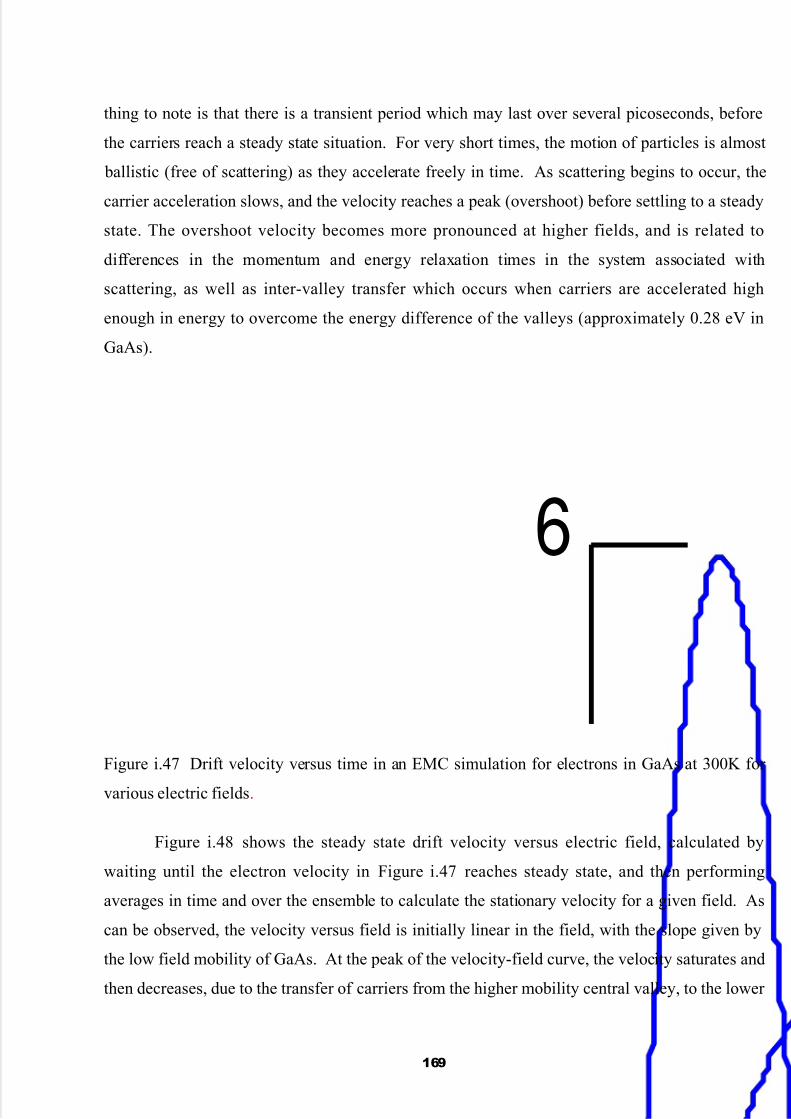
5/13/2018 eBook.comp Electronics - slidepdf.com
http://slidepdf.com/reader/full/ebookcomp-electronics 169/236
thing to note is that there is a transient period which may last over several picoseconds, before
the carriers reach a steady state situation. For very short times, the motion of particles is almost
ballistic (free of scattering) as they accelerate freely in time. As scattering begins to occur, the
carrier acceleration slows, and the velocity reaches a peak (overshoot) before settling to a steady
state. The overshoot velocity becomes more pronounced at higher fields, and is related to
differences in the momentum and energy relaxation times in the system associated with
scattering, as well as inter-valley transfer which occurs when carriers are accelerated high
enough in energy to overcome the energy difference of the valleys (approximately 0.28 eV in
GaAs).
6
Figure i.47 Drift velocity versus time in an EMC simulation for electrons in GaAs at 300K for
various electric fields.
Figure i.48 shows the steady state drift velocity versus electric field, calculated by
waiting until the electron velocity in Figure i.47 reaches steady state, and then performing
averages in time and over the ensemble to calculate the stationary velocity for a given field. As
can be observed, the velocity versus field is initially linear in the field, with the slope given by
the low field mobility of GaAs. At the peak of the velocity-field curve, the velocity saturates and
then decreases, due to the transfer of carriers from the higher mobility central valley, to the lower
169

5/13/2018 eBook.comp Electronics - slidepdf.com
http://slidepdf.com/reader/full/ebookcomp-electronics 170/236
mobility satellite valleys. This mechanism is responsible for a region of negative resistance and
corresponding Gunn oscillations due to the ensuing instability associate with negative resistance.
2
x 1
Figure i.48 Average drift velocity versus electric field for Bulk GaAs at 300K.
5.7.Multi-Carrier Effects
Multi-particle effects relate to the interaction between particles in the system, which is a
nonlinear effect when viewed in the context of the BTE, due to the dependence of such effects on
the single particle distribution function itself. Particle-particle interactions are important in
Monte Carlo simulation in establishing or relaxing to an equilibrium distribution function
characterized by a Maxwell-Boltzman distribution for non-degenerate situations, or a Fermi-
Dirac when proper account for the Pauli exclusion principle is included. Most algorithms
developed to deal with such effects essentially linearize the BTE by using the previous value of
the distribution function to determine the time evolution of a particle over the successive time-step. Multi-carrier effects may range from simple consideration of the Pauli exclusion principle
(which depends on the exact occupancy of states in the system), to single particle and collective
excitations in the system. Inclusion of carrier-carrier interactions in Monte Carlo simulation has
been an active area of research for quite some time and is briefly discussed below. Another
carrier-carrier effect that is of considerable importance when estimating leakage currents for
170

5/13/2018 eBook.comp Electronics - slidepdf.com
http://slidepdf.com/reader/full/ebookcomp-electronics 171/236
example in MOSFET devices, is impact ionization, which is a pure generation process involving
three particles (two electrons and a hole or two holes and an electron). The latter is also
discussed below.
5.7.1. Pauli exclusion principle
The Pauli exclusion principle requires that the bare scattering rate given by Eq. (6.13) be
modified by a factor ( )k ′− m f 1 in the collision integral of the BTE, where ( )k ′m f is the one-
particle distribution function for the state k ′ in band (subband) m after scattering. Since the net
scattering rate including the Pauli exclusion principle is always less than the bare scattering rate,
a self-scattering rejection technique may be used in the Monte Carlo simulation as proposed by
Bosi and Jacoboni [88] for one particle simulation and extended by Lugli and Ferry [89] for EMC.
In the self-scattering rejection algorithm, an additional random number r is generated (between 0
and 1), and this number is compared to ( )k ′m f , the occupancy of the final state (which is also
between 0 and 1 when properly normalized for the numerical k -space discretization). If r is
greater than ( )k ′m f , the scattering is accepted and the particle’s momentum and energy are
changed. If this condition is not satisfied, the scattering is rejected, and the process is treated as
a self-scattering event with no change of energy or momentum after scattering. Through this
algorithm, no scattering to this state can occur if the state is completely full.
5.7.2. Carrier-carrier interactions
Carrier-carrier scattering, may be treated as a scattering process within the Monte Carlo
algorithm on the same footing as other mechanisms. In the simplest case of bulk electrons in a
single parabolic conduction band, the process may be treated as a binary collision where the
scattering rate for a particle of wavevector k 0 due to all the other particles in the ensemble is
given by [90]
171

5/13/2018 eBook.comp Electronics - slidepdf.com
http://slidepdf.com/reader/full/ebookcomp-electronics 172/236
( ) ( )( )22
0
0
223
4
04 β β ε π +−
−=Γ ∫
k k
k k k k k f d
enmnee , (i.246)
where f (k ) is the one-particle distribution function (normalized to unity), ε is the permittivity, nis the electron density, and β is the screening constant. In deriving Eq. (6.15), one assumes that
the two particles interact through a statically screened Coulomb interaction, which ignores the
energy exchange between particles in the screening which in itself is a dynamic, frequency-
dependent effect. Similar forms have been derived for electrons in 2D [91,92] and 1D [93], where
carrier-carrier scattering leads to inter-subband as well as intra-subband transitions. Since the
scattering rate in Eq. (6.15) depends on the distribution function of all the other particles in the
system, this process represents a nonlinear term as mentioned earlier. One method is to tabulate
f (k ) on a discrete grid, as is done for the Pauli principle, and then numerically integrate Eq.
(6.15) at each time step. An alternate method is to use a self-scattering rejection technique [94],
where the integrand excluding f (k ) is replaced by its maximum value and taken outside the
integral over k . The integral over f (k ) is just unity, giving an analytic form used to generate the
free flight. Then, the self-scattering rejection technique is used when the final state is chosen to
correct for the exact scattering rate compared to this artificial maximum rate, similar to the
algorithm used for the Pauli principle.
The treatment of intercarrier interactions as binary collisions above neglects scattering by
collective excitations such as plasmons or coupled plasmon-phonon modes. These effects may
have a strong influence on carrier relaxation, particularly at high carrier density. One approach
is to make a separation of the collective and single particle spectrum of the interacting many-
body Hamiltonian, and treat them separately, i.e. as binary collisions for the single particle
excitations, and as electron-plasmon scattering for the collective modes [95]. Another approach is
to calculate the dielectric response within the random phase approximation, and associate the
damping given by the imaginary part of the inverse dielectric function with the electron lifetime
[96].
A semiclassical approach to carrier-carrier interaction, which is fully compatible with the
Monte Carlo algorithm, is the use of Molecular Dynamics [97], in which carrier-carrier interaction
172

5/13/2018 eBook.comp Electronics - slidepdf.com
http://slidepdf.com/reader/full/ebookcomp-electronics 173/236
is treated continuously in real space during the free-flight phase through the Coulomb force of all
the particles. A very small time step is required when using Molecular Dynamics to account for
the dynamic distribution of the system. A time step on the order of 0.5 fs is often sufficiently
small for this purpose. The small time step assures that the forces acting on the particles during
the time of flight are essentially constant, that is f t f t t ( ) ( )≅ + ∆ , where f (t ) is the single
particle distribution function.
Using Newtonian kinematics, we can write the real space trajectories of each particle as
( ) ( ) 2)(
2
1t
m
t t t t t ∆+∆+=∆+
Fvrr , (i.247)
and( ) ( )
( )t
m
t t t t ∆+=∆+
Fvv . (i.248)
Here, F(t ) is the force arising from the applied field as well as that of the Coulomb interactions.
We can write F(t ) as
( ) ( )( )
∇−= ∑
i
i t qt rEF ϕ , (i.249)
where qE is the force due to the applied field and the summation is the interactive force due to
all particles separated by distance ri , with ϕ (ri ) the electrostatic potential. As in Monte Carlo
simulation, one has to simulate a finite number of particles due to practical computational
limitations on execution time. In real space, this finite number of particles corresponds to a
particular simulation volume given a certain density of carriers, n N V /= , where n is the
density. Since the carriers can move in and out of this volume, and since the Coulomb
interaction is a long-range force, one must account for the region outside V by periodically
replicating the simulated system. The contributions due to the periodic replication of the
particles inside V in cells outside has a closed form solution in the form of an Ewald sum [98],
which gives a linear as well as 1/r 2 contribution to the force. The equation for the total force in
the Molecular Dynamics technique then becomes
173

5/13/2018 eBook.comp Electronics - slidepdf.com
http://slidepdf.com/reader/full/ebookcomp-electronics 174/236
∑
+
−=
N
i
ii
iV
era
rF
3
21
4 2
2 π
π ε . (i.250)
The above equation is easily incorporated in the standard Monte Carlo simulationdiscussed up to this point. At every time step the forces on each particle due to all the other
particles in the system are calculated from Eq. (6.19). From the forces, an interactive electric
field is obtained which is added to the external electric field of the system to couple the
Molecular Dynamics to the Monte Carlo.
The inclusion of the carrier-carrier interactions in the context of particle-based device
simulations is discussed in Section ??. The main difficulty in treating this interaction term in
device simulations arises from the fact that the long-range portion of the carrier-carrier
interaction is included via the numerical solution of the quasi-static Poisson equation. Under
these circumstances, special care has to be taken when incorporating the short-range portion of
this interaction term to prevent double counting of the force.
5.7.3. Band to Band Impact Ionization
Another carrier-carrier scattering process is that of impact ionization, in which an
energetic electron (or hole) has sufficient kinetic energy to create an electron-hole pair. Impactionization therefore leads to the process of carrier multiplication. This process is critical for
example in the avalanche breakdown of semiconductor junctions, and is a detrimental effect in
short channel MOS devices in terms of excess substrate current and decreased reliability.
The ionization rate of valence electrons by energetic conduction band electrons is usually
described by Fermi’s rule Eq. (6.14), in which a screened Coulomb interaction is assumed
between the two particles, as discussed earlier in this section, where screening is described by an
appropriate dielectric function such as that proposed by Levine and Louie [99]. In general, theimpact ionization rate should be a function of the wavevector of the incident electron, hence of
the direction of an electric field in the crystal, although there is still some debate as to the
experimental and theoretical evidence. More simply, the energy dependent rate (averaged over
all wavevectors on a constant energy shell) may be expressed analytically in the power law form
174

5/13/2018 eBook.comp Electronics - slidepdf.com
http://slidepdf.com/reader/full/ebookcomp-electronics 175/236
( ) [ ]a
thii E E P E −=Γ , (i.251)
where E th is the threshold energy for the process to occur, which is determined by momentum
and energy conservation considerations, but minimally is the bandgap of the material itself. P and a are parameters which may be fit to more sophisticated models. The Keldysh formula [100]
is derived by expanding the matrix element for scattering close to threshold, which gives a=2,
and the constant P =C/E th2 , with C =1.19× 10¹⁴/s and assuming a parabolic band approximation,
g
cv
cvth E
mm
mm E
/1
/23
−−
= , (i.252)
where mv and mc are the effective masses of the valence and conduction band respectively, and E g
is the bandgap. More complete full-bandstructure calculations of the impact ionization rate have
been reported for Si [101,102], GaAs [102,103] and wide bandgap materials [104], which are fairly
well fit using power law model given in Eq. (6.18).
Within the ensemble Monte Carlo method, the maximum scattering rate is used to
generate the free flight time. The state after scattering of the initial electron plus the additional
electron and hole must satisfy both energy and momentum conservation within the Fermi rule
model, which is somewhat complicated unless simple parabolic band approximations are made.
5.7.4. Full-Band Particle Based Simulation
The Monte Carlo algorithm discussed in this section initially evolved during the 1970s
and early 1980s using simplified representations of the electronic bandstructure in terms of a
multi-valley parabolic or non-parabolic approximation close to band minima and maxima. This
simplifies the particle tracking in terms of the E-k relationship and particle motion in real space,
and greatly simplifies the calculated scattering rates such that analytical forms may be used. It
soon became apparent that for devices where high field effects are important, or for the correct
simulation of high energy processes like impact ionization, the full band structure of the material
is required. Particle based simulation which incorporates part or all of the band structure directly
175

5/13/2018 eBook.comp Electronics - slidepdf.com
http://slidepdf.com/reader/full/ebookcomp-electronics 176/236
into the particle dynamics and scattering is commonly referred to as full-band Monte Carlo
simulation [83].
Typically, the Empirical Pseudopotential Method (EPM)[105] has been utilized in full
band Monte Carlo codes due to the relative simplicity of the calculation, and the plane wave
basis which facilitates calculation of some scattering processes. Early full band codes developed
at the University of Illinois utilized the full bandstructure for the particle dynamics, but assumed
isotropic energy dependent scattering rates using the full band density of states [83]. This is due
to the computational difficulty and memory requirements to store the full k -dependent scattering
rates throughout the whole Brillouin zone. Later simulators relaxed this restriction, although
often assuming quasi-isotropic rates. Probably the most completely developed full-band code for
full-band Monte Carlo device simulation is the DAMOCLES code developed at IBM byFischetti and Laux [106], which has been used extensively for simulation of a variety of device
technologies [107].
The full-band codes above are based on essentially the same algorithm as discussed
above, in which a particle scatters based on the total scattering rate, then the type of scattering
and the final state after scattering are selected using the full k-dependent rates for each
mechanism. An alternative approach, referred to as Cellular Monte Carlo [108], stores the entire
transition table for the total scattering rate for all mechanisms from every initial state k to every
final state k’ . Particle scattering is accomplished in a single step, at the expense of large memory
consumption (on the order of 2Gbytes of RAM) necessary to store the necessary scattering
tables.
176
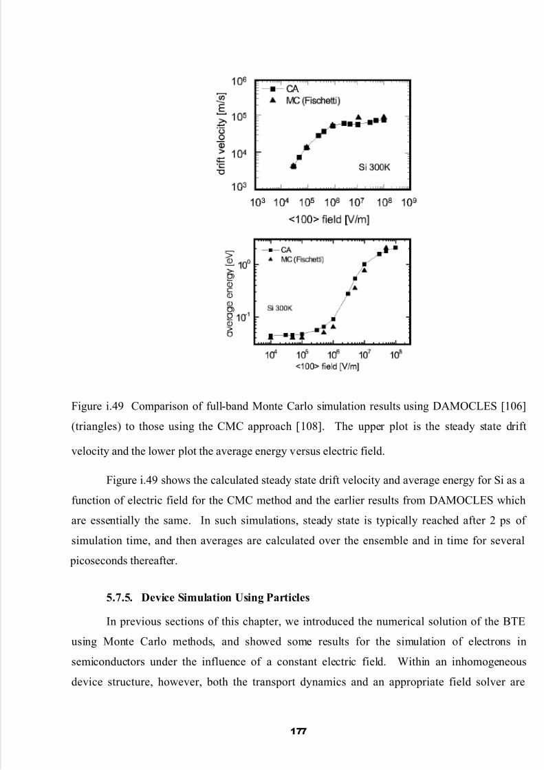
5/13/2018 eBook.comp Electronics - slidepdf.com
http://slidepdf.com/reader/full/ebookcomp-electronics 177/236
Figure i.49 Comparison of full-band Monte Carlo simulation results using DAMOCLES [106]
(triangles) to those using the CMC approach [108]. The upper plot is the steady state drift
velocity and the lower plot the average energy versus electric field.
Figure i.49 shows the calculated steady state drift velocity and average energy for Si as a
function of electric field for the CMC method and the earlier results from DAMOCLES which
are essentially the same. In such simulations, steady state is typically reached after 2 ps of
simulation time, and then averages are calculated over the ensemble and in time for several
picoseconds thereafter.
5.7.5. Device Simulation Using Particles
In previous sections of this chapter, we introduced the numerical solution of the BTE
using Monte Carlo methods, and showed some results for the simulation of electrons in
semiconductors under the influence of a constant electric field. Within an inhomogeneous
device structure, however, both the transport dynamics and an appropriate field solver are
177

5/13/2018 eBook.comp Electronics - slidepdf.com
http://slidepdf.com/reader/full/ebookcomp-electronics 178/236
coupled to each other. For quasi-static situations, as discussed in earlier chapters, the spatially
varying fields associated with the potential arising from the numerical solution of Poisson's
equation are the driving force accelerating particles in the Monte Carlo phase. Likewise, the
distribution of mobile (both electrons and holes) and fixed charges (e.g. donors and acceptors)
provides the source of the electric field in Poisson's equation corresponding to the right-hand
side of Eq. (??). By decoupling the transport portion from the field portion over a small time
interval (discussed in more detail below), a convergent scheme is realized in which the Monte
Carlo transport phase is self-consistently coupled to Poisson’s equation, similar to Gummel’s
algorithm discussed in Chapter 2. In the following section, a description of Monte Carlo
particle-based device simulators is given, with emphasis on the particle-mesh coupling and the
inclusion of the short-range Coulomb interactions.
5.8.Device Simulation Using Particles
In previous sections of this chapter, we introduced the numerical solution of the BTE
using Monte Carlo methods, and showed some results for the simulation of electrons in
semiconductors under the influence of a constant electric field. Within an inhomogeneous
device structure, however, both the transport dynamics and an appropriate field solver are
coupled to each other. For quasi-static situations, as discussed in earlier chapters, the spatially
varying fields associated with the potential arising from the numerical solution of Poisson'sequation are the driving force accelerating particles in the Monte Carlo phase. Likewise, the
distribution of mobile (both electrons and holes) and fixed charges (e.g. donors and acceptors)
provides the source of the electric field in Poisson's equation corresponding to the right-hand
side of Eq. (??). By decoupling the transport portion from the field portion over a small time
interval (discussed in more detail below), a convergent scheme is realized in which the Monte
Carlo transport phase is self-consistently coupled to Poisson’s equation, similar to Gummel’s
algorithm discussed in Chapter 3. In the following section, a description of Monte Carlo
particle-based device simulators is given, with emphasis on the particle-mesh coupling and the
inclusion of the short-range Coulomb interactions.
178

5/13/2018 eBook.comp Electronics - slidepdf.com
http://slidepdf.com/reader/full/ebookcomp-electronics 179/236
5.8.1. Monte Carlo Device Simulation
As mentioned above, for device simulation based on particles, Poisson's equation is
decoupled from the particle motion (described e.g. by the EMC algorithm) over a suitably small
time step, typically less than the inverse plasma frequency corresponding to the highest carrier density in the device. Over this time interval, carriers accelerate according to the frozen field
profile from the previous time-step solution of Poisson's equation, and then Poisson's equation is
solved at the end of the time interval with the frozen configuration of charges arising from the
Monte Carlo phase (see discussion in Ref. [97]). It is important to note that Poisson's equation is
solved on a discrete mesh, whereas the solution of charge motion using EMC occurs over a
continuous range of coordinate space in terms of the particle position. An illustration of a typical
device geometry and the particle mesh scheme is shown in Figure i.50. Therefore, a particle-
mesh (PM) coupling is needed for both the charge assignment and the force interpolation. The
size of the mesh and the characteristic time scales of transport set constraints on both the time-
step and mesh size. We must consider how particles are treated in terms of the boundaries, and
how they are injected. Finally, the determination of the charge motion and corresponding
terminal currents from averages over the simulation results are necessary in order to calculate the
I-V characteristics of a device. These issues are discussed in detail below, along with some
typical simulation results.
Figure i.50. Schematic diagram of a prototypical three-terminal device where charge flow isdescribed by particles, while the fields are solved on a finite mesh.
179

5/13/2018 eBook.comp Electronics - slidepdf.com
http://slidepdf.com/reader/full/ebookcomp-electronics 180/236
Time-Step and Grid Size Considerations
As in the case of any time domain simulation, for stable Monte Carlo device simulation,
one has to choose the appropriate time step, ∆ t , and the spatial mesh size (∆ x, ∆ y, and/or ∆ z ).
The time step and the mesh size may correlate to each other in connection with the numericalstability. For example, the time step ∆ t must be related to the plasma frequency
*
2
m
ne
s p ε
=ω , (i.253)
where n is the carrier density. From the viewpoint of numerical stability, ∆ t must be much
smaller than the inverse plasma frequency above. Since the inverse plasma frequency goes as
n/1 , the highest carrier density occurring in the modeled device structure corresponds to the
smallest time used to estimate ∆ t . If the material is a multi-valley semiconductor, the smallest
effective mass encountered by the carriers must be used in Eq. (6.22) as well. For example, in
the case of electrons in the central valley of GaAs ( omm 067.0* = ), a doping of 5× 1017 cm-3
corresponds to ω p ≅ 5× 10¹³; hence, ∆ t must be smaller than 0.02 ps.
The mesh size for the spatial resolution of the potential is dictated by the spatial variationof charge variations. Hence, one has to choose the mesh size to be smaller than the smallest
wavelength of the charge variations. The smallest wavelength is approximately equal to the
Debye length (for degenerate semiconductors the relevant length is the Thomas-Fermi
wavelength), given by
ne
T k B s D 2
ε=λ . (i.254)
Again, due to the inverse dependence of this length on the square root of the density, the highest
carrier density modeled should be used to estimate Dλ for stability. Hence, the mesh size must
be chosen to be smaller than the Debye length given by Eq. (6.21). Again, for the case of GaAs,
with a doping density of 5× 1017 cm-3, Dλ ≅ 6 nm.
180

5/13/2018 eBook.comp Electronics - slidepdf.com
http://slidepdf.com/reader/full/ebookcomp-electronics 181/236
Based on the discussion above, the time step (∆ t ), and the mesh size (∆ x, ∆ y, an/or
∆ z ) are chosen independently based on the physical arguments given above. However, there are
numerical constraints coupling both as well. More specifically, the relation of ∆ t to the grid size
must also be checked by calculating the distance l max
, defined as
t l ∆×= maxmax v , (i.255)
where vmax is the maximum carrier velocity, that can be approximated by the maximum group
velocity of the electrons in the semiconductor (on the order of 108 cm/s). The distance l max is the
maximum distance the carriers can propagate during ∆ t . The time step is therefore chosen to be
small enough so that l max is smaller than the spatial mesh size chosen using Eq. (6.21). This
constraint arises because for too large of a time step, ∆ t , there may be substantial change in the
charge distribution, while the field distribution in the simulation is only updated every ∆ t ,
leading to unacceptable errors in the carrier force.
181
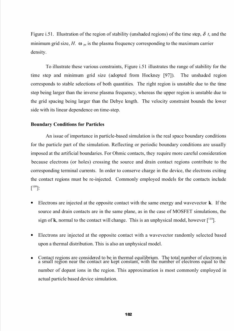
5/13/2018 eBook.comp Electronics - slidepdf.com
http://slidepdf.com/reader/full/ebookcomp-electronics 182/236
Figure i.51. Illustration of the region of stability (unshaded regions) of the time step, δ t , and the
minimum grid size, H . ω pe is the plasma frequency corresponding to the maximum carrier
density.
To illustrate these various constraints, Figure i.51 illustrates the range of stability for the
time step and minimum grid size (adopted from Hockney [97]). The unshaded region
corresponds to stable selections of both quantities. The right region is unstable due to the time
step being larger than the inverse plasma frequency, whereas the upper region is unstable due to
the grid spacing being larger than the Debye length. The velocity constraint bounds the lower
side with its linear dependence on time-step.
Boundary Conditions for Particles
An issue of importance in particle-based simulation is the real space boundary conditions
for the particle part of the simulation. Reflecting or periodic boundary conditions are usually
imposed at the artificial boundaries. For Ohmic contacts, they require more careful consideration
because electrons (or holes) crossing the source and drain contact regions contribute to the
corresponding terminal currents. In order to conserve charge in the device, the electrons exiting
the contact regions must be re-injected. Commonly employed models for the contacts include
[109]:
• Electrons are injected at the opposite contact with the same energy and wavevector k . If the
source and drain contacts are in the same plane, as in the case of MOSFET simulations, the
sign of k , normal to the contact will change. This is an unphysical model, however [110].
• Electrons are injected at the opposite contact with a wavevector randomly selected based
upon a thermal distribution. This is also an unphysical model.
• Contact regions are considered to be in thermal equilibrium. The total number of electrons ina small region near the contact are kept constant, with the number of electrons equal to the
number of dopant ions in the region. This approximation is most commonly employed in
actual particle based device simulation.
182

5/13/2018 eBook.comp Electronics - slidepdf.com
http://slidepdf.com/reader/full/ebookcomp-electronics 183/236
• Another method uses ‘reservoirs’ of electrons adjacent to the contacts. Electrons naturally
diffuse into the contacts from the reservoirs, which are not treated as part of the device
during the solution of Poisson’s equation. This approach gives results similar to the velocity-
weighted Maxwellian, but at the expense of increased computational time due to the extra
electrons simulated. It is an excellent model employed in some of the most sophisticated
particle-based simulators. There are also several possibilities for the choice of the
distribution function Maxwellian, displaced Maxwellian, and velocity-weighted
Maxwellian [111].
Particle-mesh (PM) coupling
The particle-mesh (PM) coupling is broken into four steps: (1) assignment of particle
charge to the mesh; (2) solution of Poisson’s equation on the mesh; (3) calculation of the mesh-
defined forces; and (4) interpolation to find the forces acting on the particle. The charge
assignment and force interpolation schemes usually employed in self-consistent Monte Carlo
device simulations are the nearest-grid-point (NGP) and the cloud-in-cell (CIC) schemes [112].
Figure i.52 illustrates both methods. In the NGP scheme, the particle position is mapped into the
charge density at the closest grid point to a given particle. This has the advantage of simplicity,
but leads to a noisy charge distribution, which may exacerbate numerical instability. Alternately,
within the CIC scheme a finite volume is associated with each particle spanning several cells inthe mesh, and a fractional portion of the charge per particle is assigned to grid points according
to the relative volume of the ‘cloud’ occupying the cell corresponding to the grid point. This
method has the advantage of smoothing the charge distribution due to the discrete charges of the
particle based method, but may result in an artificial ‘self-force’ acting on the particle,
particularly if an inhomogeneous mesh is used.
183

5/13/2018 eBook.comp Electronics - slidepdf.com
http://slidepdf.com/reader/full/ebookcomp-electronics 184/236
N G P C I CFigure i.52. Illustration of the charge assignment based on the nearest grid point method (NGP)and the cloud in cell method (CIC).
To better understand the NGP and the CIC scheme, consider a tensor product mesh with
mesh lines xi N i x ,,1, = and y j N j y ,,1, = . If the mesh is uniformly spaced in each axis
direction, then ( ) ( )121 +++ −=− l l l l x x x x . The permittivities are considered constant within each
mesh element and are denoted by 1,,1, −=ε xkl N k and 1,,1 −= y N l . Define centered
finite-differences of the potential ψ in the x- and y-axis at the midpoints of element edges as
follows:
−−
−=∆
−−
−=∆
+
++
+
+
+
,
,
1
,1,
1
,,1
2
1,
,21
l l
l k l k y
k k
l k l k x
y y
x x
l k
l k
ψ ψ
ψ ψ
(i.256)
where the minus sign is included for convenience because the electric field is negative of the
gradient of the potential. Consider now a point charge in 2-D located at ),( y x within an
element ji, . If the restrictions for the permittivity (P) and the tensor-product meshes with
184

5/13/2018 eBook.comp Electronics - slidepdf.com
http://slidepdf.com/reader/full/ebookcomp-electronics 185/236
uniform spacing in each direction (M) apply, the standard NGP/CIC schemes in two dimensions
can be summarized by the following four steps:
(1) Charge assignment to the mesh: The portion of the charge Lρ assigned to the element
nodes (k ,l ) is Lkl w ρ , k =i, i+1 and l = j, j+1, where kl w are the four charge weights which
sum to unity by charge conservation. For the NGP scheme, the node closest to ( x, y)
receives a weight kl w =1, with the remaining three weights set to zero. For the CIC
scheme, the weights are y xij www = , ( ) y x ji www −=+ 1,1 , ( y x ji www −=+ 11, , and
( ) y x ji www −−=++ 111,1 , ( ) ( )iii x x x x xw −−= ++ 11 / and j j j y y y y yw −−= ++ 11 / .
(2) Solve the Poisson equation: The Poisson equation is solved by some of the numerical
techniques discussed in Appendix A.(3) Compute forces on the mesh: The electric field at mesh nodes (k ,l ) is computed as:
2/,,
21
21
∆+∆= +−
xl k
xl k
xkl E and 2/
21
21 ,,
∆+∆=
+− y
l k
y
l k
ykl E , for k = i, i+1 and l= j, j+1.
(4) Interpolate to find forces on the charge: Interpolate the field to position ( x, y) according to
∑= kl xkl kl
x E w E and ∑= kl
ykl kl
y E w E , where k = i, i+1, l = j, j+1 and the ijw are the
NGP or CIC weights from step 1.
The requirements (P) and (M) severely limit the scope of devices that may be considered in
device simulations using the NGP and the CIC schemes. Laux [113] proposed a new particle-
mesh coupling scheme, namely, the nearest-element-center (NEC) scheme, which relaxes the
restrictions (P) and (M). The NEC charge assignment/force interpolation scheme attempts to
reduce the self-forces and increase the spatial accuracy in the presence of nonuniformly spaced
tensor-product meshes and/or spatially-dependent permittivity. In addition, the NEC scheme can
be utilized in one axis direction (where local mesh spacing is nonuniform) and the CIC scheme
can be utilized in the other (where local mesh spacing is uniform). Such hybrid schemes offer
smoother assignment/interpolation on the mesh compared to the pure NEC. The new steps of the
pure NEC PM scheme are:
185

5/13/2018 eBook.comp Electronics - slidepdf.com
http://slidepdf.com/reader/full/ebookcomp-electronics 186/236
(1') Charge assignment to the mesh: Divide the line charge Lρ equally to the four mesh points
of the element ji, .
(3') Compute forces on the mesh: Calculate the fields x
l i ,21+∆ , l= j, j+1, and
y
jk 21, +
∆ , k=i, i+1.
(4') Interpolate to find force on the charge: Interpolate the field according to the following
2/1,,
21
21
∆+∆= +++
x
ji
x
ji
x E and 2/
21
21 ,1,
∆+∆= +++
x ji
x ji
y E .
The NEC designation derives from the appearance, in step (1') of moving the charge to
the center of its element and applying a CIC-like assignment scheme. The NEC scheme involves
only one mesh element and its four nodal values of potential. This locality makes the method
well-suited to non-uniform mesh spacing and spatially-varying permittivity. The interpolationand error properties of the NEC scheme are similar to the NGP scheme.
Real Space Trajectories of Particles
The motion in real space of particles under the influence of electric fields is somewhat
more complicated due to the band structure. Recalling the discussion in Chapter 1 the velocity
of a particle in real space is related to the E -k dispersion relation defining the bandstructure as
( ) ( )( )
( )
rEk
k rv k
q
dt
d
t E dt d t
=
∇== 1
(i.257)
where the rate of change of the crystal momentum is related to the local electric field acting on
the particle through the acceleration theorem expressed by the second equation. In turn, the
change in crystal momentum, k (t ), is related to the velocity through the gradient of E with
respect to k. If one has to use the full bandstructure of the semiconductor, then integration of
these equations to find r(t ) is only possible numerically, using for example a Runge-Kutta
algorithm[79]. If a three valley model with parabolic bands is used, then the expression is
integrable
186

5/13/2018 eBook.comp Electronics - slidepdf.com
http://slidepdf.com/reader/full/ebookcomp-electronics 187/236
( )
rEk k rv
q
d t
d
md t
d === ;
*(i.258)
Therefore, for a constant electric field in the x direction, the change in distance along the x
direction is found by integrating twice
( ) ( ) ( )*2
00
20
m
t q E t v xt x x
x ++= (i.259)
Simulated Device Behavior
To simulate the steady-state behavior of a device, the system must be initialized in some
initial condition, with the desired potentials applied to the contacts, and then the simulation
proceeds in a time stepping manner until steady-state is reached. This process may take several
picoseconds of simulation time, and consequently several thousand time-steps based on the usual
time increments required for stability. Clearly, the closer the initial state of the system is to the
steady state solution, the quicker the convergence. If one is, for example, simulating the first
bias point for a transistor simulation, and has no a priori knowledge of the solution, a common
starting point for the initial guess is to start out with charge neutrality, i.e. to assign particles
randomly according to the doping profile in the device and based on the super-particle charge
assignment of the particles, so that initially the system is charge neutral on the average. For two-
dimensional device simulation, one should keep in mind that each particle actually represents a
rod of charge into the third dimension. Subsequent simulations at the same device at different
bias conditions can use the steady state solution at the previous bias point as a good initial guess.
After assigning charges randomly in the device structure, charge is then assigned to each mesh
point using the NGP or CIC particle-mesh methods, and Poisson’s equation solved. The forces
are then interpolated on the grid, and particles are accelerated over the next time step. A flow-chart of a typical Monte Carlo device simulation is shown in Figure i.53.
187

5/13/2018 eBook.comp Electronics - slidepdf.com
http://slidepdf.com/reader/full/ebookcomp-electronics 188/236
Figure i.53 Flow chart of a typical particle based device simulation.
As the simulation evolves, charge will flow in and out of the contacts, and depletion
regions internal to the device will form until steady state is reached. The charge passing through
188

5/13/2018 eBook.comp Electronics - slidepdf.com
http://slidepdf.com/reader/full/ebookcomp-electronics 189/236
the contacts at each time step can be tabulated, and a plot of the cumulative charge as a function
of time plotted as shown in Figure i.54. Here a n-channel GaAs metal semiconductor field effect
transistor (MESFET) device with a Schottky gate is simulated [ 114]. The Schottky gate is simply
modeled as absorbing all carriers from the semiconductor side that have sufficient energy to
overcome the potential barrier there, but they are not re-emitted back into the semiconductor, as
opposed to the Ohmic contact case. For the particle dynamics, a simply three valley model for
GaAs is used including polar optical phonons, intervalley phonon scattering, and impurity
scattering. As can be seen, carriers flow out of the gate and drain, and flow in from the source,
until a depletion region is established under Schottky gate after about 4 ps. In steady state, the
charge versus time is linear, the slope of the source or drain contacts corresponding to the source
drain current, while the gate current is approximately zero.
Figure i.54. Plot of the cumulative charge through the source, drain, and gate simulations as a
function of time during the simulation for a GaAs MESFET device.
Figure i.55 shows the particle distribution in 3D of a MESFET, where the dots indicate
the individual simulated particles for two different gate biases. Here the heavily doped MESFET
region (shown by the inner box) is surrounded by semi-insulating GaAs forming the rest of the
simulation domain. The upper curve corresponds to no net gate bias (i.e. the gate is positively
189

5/13/2018 eBook.comp Electronics - slidepdf.com
http://slidepdf.com/reader/full/ebookcomp-electronics 190/236
biased to overcome the built-in potential of the Schottky contact), while the lower curve
corresponds to a net negative bias applied to the gate, such that the channel is close to pinchoff.
One can see the evident depletion of carriers under the gate under the latter conditions.
Figure i.55. Example of the particle distribution in a MESFET structure simulated in 3D using
an EMC approach. The upper plot is the device with zero gate voltage applied, while the lower
is with a negative gate voltage applied, close to pinch-off.
After sufficient time has elapsed, so that the system is driven into a steady-state regime,
one can calculate the steady-state current through a specified terminal. The device current can be
determined via two different, but consistent methods. First, by keeping track of the charges
entering and exiting each terminal, as was done above, the net number of charges over a period
of the simulation can be used to calculate the terminal current. This method, however, is
190

5/13/2018 eBook.comp Electronics - slidepdf.com
http://slidepdf.com/reader/full/ebookcomp-electronics 191/236
relatively noisy due to the discrete nature of the carriers, and the fact that one is only counting
the currents crossing a 2D boundary in the device, which limits the statistics. A second method
uses the sum of the carrier velocities in a portion of the device are used to calculate the current.
For this purpose, the device is divided into several sections along, for example, the x-axis (from
source to drain for the case of a MOSFET or MESFET simulation). The number of carriers and
their corresponding velocity is added for each section after each free-flight time step. The total
x-velocity in each section is then averaged over several time steps to determine the current for
that section. The total device current can be determined from the average of several sections,
which gives a much smoother result compared to counting the terminal charges. By breaking the
device into sections, individual section currents can be compared to verify that the currents are
uniform. In addition, sections near the source and drain regions of a MOSFET or a MESFET
may have a high y-component in their velocity and should be excluded from the current
calculations.
As a more specific example of calculated current-voltage (I-V) characteristics of a
device, Figure i.56 shows the cross-section of a semiconductor on insulator MOS technology,
where a buried oxide (BOX) is created by ion-implantation of oxygen or some other process.
The top layer is typically Si, although more recently Ge top layers have been of interest. A two-
dimenional device simulation based on the computational domain represented by the dashed
curve has been performed [115]. Due to the anisotropic and multi-band nature of the valence band
shown in Figure 6.16b, a full-band Cellular Monte Carlo simulation was performed for hole
transport in the channel of these devices.
191

5/13/2018 eBook.comp Electronics - slidepdf.com
http://slidepdf.com/reader/full/ebookcomp-electronics 192/236
I n s u l a t o r
S i l i c o n s u b
G a t eS o u r c e D r a
V B
p
+
p
+n
V G V D
I n s u l a t o r
S i l i c o n s u b
G a t eS o u r c e D r a
V B
p
+
p
+n
V G V D
a) b)
Figure i.56. a) Cross-section of a p-channel Semiconductor on Insulator (SOI) field effect
transistor; b) constant energy surfaces for the top of the valence band in Ge [115].
Figure i.57 shows the calculated ISD-VSD characteristics for various gate biases relative to
the threshold voltage. Here, a 297× 65 and 337× 65 tensor product grid was used for the solution
of Poisson’s equation for the 90 nm and 130 nm devices, respectively. 80,000 super-particles
were used in these simulations with a 0.2 fs timestep. The current was calculated through
averages over slices in the channel, as discussed earlier. As can be seen, the statistical
fluctuation of the calculated curves is relatively small, and systematic differences between Ge on
insulator versus Si on insulator are found, due to the higher hole mobility of Ge versus Si.
192

5/13/2018 eBook.comp Electronics - slidepdf.com
http://slidepdf.com/reader/full/ebookcomp-electronics 193/236
. . . . ..
.
.
.
.
.
.
.
.
.
I
I
- 2 . 0 - 1 . 5 - 1 . 0 - 0 . 5 0 . 00 . 0
0 . 5
1 . 0
1 . 5
2 . 0
2 . 5
- 2 . 0 - 1 . 5 - 1 . 0 - 0 . 5 0 . 00 . 0
0 . 5
1 . 0
1 . 5
2 . 0
2 . 5
3 . 01 3 0 n m S O I
1 3 0 n m G O I
9 0 n m
9 0 n m
D r a i n V o l t a g eD S
V - V = - 1 . 5 VG T
V - V = - 1 . 0 VG T
V - V = - 0 . 5 VG T
D
r a
i n
C
u
r r e
n
t
D
e
n
s
i t y
[ m
A
/
m
]
µ
D r a i n V o l t a g e V [ V ]D S
V - V = - 0 . 5 VG T
V - V = - 1 . 0 VG T
V - V = - 1 . 5 VG T
D
r a
i n
C
u
r r e
n
t
D
e
n
s
i t y
[ m
A
/
m
]
µ
Figure i.57. Calculated I-V characteristics for the p-channel SOI MOSFET structure shown in
Figure i.56 for both Ge on insulator and Si on insulator devices, for 130 and 90 nm gate lengths.
5.8.2. Direct Treatment of Inter-Particle Interaction
In modern deep-submicrometer devices, for achieving optimum device performance and
eliminating the so-called punch-through effect, the doping densities must be quite high. This
necessitates a careful treatment of the electron-electron (e-e) and electron-impurity (e-i)
interactions, an issue that has been a major problem for quite some time. Many of the approaches
used in the past have included the short-range portions of the e-e and e-i interactions in the k -space portion of the Monte Carlo transport kernel, as discussed in Section ??, thus neglecting
many of the important inelastic properties of these two interaction terms [116, 117]. An additional
problem with this screened scattering approach in devices is that, unlike the other scattering
processes, e-e and e-i scattering rates need to be re-evaluated frequently during the simulation
process to take into account the changes in the distribution function in time and spatially. The
calculation and tabulation of a spatially inhomogeneous distribution function may be highly CPU
and memory intensive. Furthermore, ionized impurity scattering is usually treated as a simple
two-body event, thus ignoring the multi-ion contributions to the overall scattering potential. A
simple screening model is usually used that ignores the dynamical perturbations to the Coulomb
fields caused by the movement of the free carriers. To overcome the above difficulties, several
authors have advocated coupling of the semi-classical molecular dynamics approach discussed in
Section ?? to the ensemble Monte-Carlo approach [118,119,120]. Simulation of the low field mobility
193

5/13/2018 eBook.comp Electronics - slidepdf.com
http://slidepdf.com/reader/full/ebookcomp-electronics 194/236
using such a coupled approach results in excellent agreement with the experimental data for high
substrate doping levels . However, it is proven to be quite difficult to incorporate this coupled
ensemble Monte-Carlo-molecular dynamics approach when inhomogeneous charge densities,
characteristic of semiconductor devices, are encountered . An additional problem with this
approach in a typical particle-based device simulation arises from the fact that both the e-e and e-
i interactions are already included, at least within the Hartree approximation (long-range carrier-
carrier interaction), through the self-consistent solution of the three-dimensional (3D) Poisson
equation via the PM coupling discussed in the previous section. The magnitude of the resulting
mesh force that arises from the force interpolation scheme, depends upon the volume of the cell,
and, for commonly employed mesh sizes in device simulations, usually leads to double-counting
of the force.
To overcome the above-described difficulties of incorporation of the short-range e-e and
e-i force into the problem, one can follow two different paths. One way is to use the P 3M scheme
introduced by Hockney and Eastwood [112]. An alternative to this scheme is to use the
corrected-Coulomb approach due to Gross et al . [121,122,123,124].
The P3M Method
The particle-particle-particle-mesh (P3
M) algorithms are a class of hybrid algorithmsdeveloped by Hockney and Eastwood [112]. These algorithms enable correlated systems with
long-range forces to be simulated for a large ensemble of particles. The essence of the method is
to express the interparticle forces as a sum of two component parts; the short range part Fsr ,
which is nonzero only for particle separations less than some cutoff radius re, and the smoothly
varying part F, which has a transform that is approximately band-limited. The total short-range
force on a particle Fsr is computed by direct particle-particle (PP) pair force summation, and the
smoothly varying part is approximated by the particle-mesh (PM) force calculation.
Two meshes are employed in the P3M algorithms: the charge-potential mesh and a
coarser mesh, the so-called chaining mesh. The charge potential mesh is used at different stages
of the PM calculation to store, in turn, charge density values, charge harmonics, potential
harmonics and potential values. The chaining mesh is a regular array of cells whose sides have
194

5/13/2018 eBook.comp Electronics - slidepdf.com
http://slidepdf.com/reader/full/ebookcomp-electronics 195/236
lengths greater than or equal to the cutoff radius re of the short-range force. Associated with
each cell of this mesh is an entry in the head-of-chain array: This addressing array is used in
conjunction with an extra particle coordinate, the linked-list coordinate, to locate pairs of
neighboring particles in the short-range calculation.
The particle orbits are integrated forward in time using the leapfrog scheme
t m
/ nni
ni ∆+=
++
211 p
xx , (i.260)
( t sr ii
ni
ni ∆++= −+
FFpp2/12/1 . (i.261)
The positions xi are defined at integral time-levels and momenta pi are defined at half-integral time-levels. Momenta pi are used rather than velocities for reasons of computational
economy.
To summarize, the change in momentum of particle i at each time step is determined by
the total force on that particle. Thus, one is free to choose how to partition the total force
between the short range and the smoothly varying part. The reference force F is the interparticle
force that the mesh calculation represents. For reasons of optimization, the cutoff radius of Fsr
has to be as small as possible, and therefore F to be equal to the total interparticle force down to
as small a particle separation as possible. However, this is not possible due to the limited
memory storage and the required CPU time even in the state-of-the-art computers.
The harmonic content of the reference force is reduced by smoothing. A suitable form of
reference force for a Coulombic long-range force is one which follows the point particle force
law beyond the cutoff radius r e, and goes smoothly to zero within that radius. The smoother the
decay of F(x) and the large re becomes, the more rapidly the harmonics R (k ) decay with
increasing k . Such smoothing procedure is equivalent to ascribing a finite size to the charged
particle. As a result, a straightforward method of including smoothing is to ascribe some simple
density profile S(x) to the reference interparticle force. Examples of shapes, which are used in
practice, and give comparable total force accuracy are the uniformly charged sphere, the sphere
with uniformly decreasing density, of the form
195

5/13/2018 eBook.comp Electronics - slidepdf.com
http://slidepdf.com/reader/full/ebookcomp-electronics 196/236
<
−
π=,
r
otherwise
ar r a
aS
,0
2/,2
48
)( 4 (i.262)
and the Gaussian distribution of density. The second scheme gives marginally better accuracies
in 3D simulations. Note that the cutoff radius of the short-range force implied by Eq. (6.26) is a
rather than re. In practice, one can make r significantly smaller than a, because continuity of
derivatives at r = a causes the reference force to closely follow the point particle force for radii
somewhat less than a. It has been found empirically that a good measure of the lower bound of re
is given by the cube root of the autocorrelation volume of the charge shapes, which for the case
of uniformly decreasing density gives:
aar e 7.048
53/1
≈
π≥ . (i.263)
Once the reference interparticle force F for the PM part of the calculation is chosen, the
short-range part Fsr is found by subtracting F from the total interparticle force, i.e.
Fsr = Ftot - F . (i.264)
The Corrected Coulomb Approach
This second approach is a purely numerical scheme that generates a corrected Coulomb
force look-up table for the individual e-e and e-i interaction terms. To calculate the proper short-
range force, one has to define a 3D box with uniform mesh spacing in each direction. A single
(fixed) electron is then placed at a known position within a 3D domain, while a second (target)
electron is swept along the ‘device’ in, for example, 0.2 nm increments so that it passes through
the fixed electron. The 3D box is usually made sufficiently large so that the boundary conditions
do not influence the potential solution. The electron charges are assigned to the nodes using one
of the charge-assignment schemes discussed previously . A 3D Poisson equation solver is then
used to solve for the node or mesh potentials. At self-consistency, the force on the swept
electron F= Fmesh is interpolated from the mesh or node potential. In a separate experiment, the
Coulomb force Ftot = Fcoul is calculated using standard Coulomb law. For each electron
196

5/13/2018 eBook.comp Electronics - slidepdf.com
http://slidepdf.com/reader/full/ebookcomp-electronics 197/236
separation, one then tabulates Fmesh , Fcoul and the difference between the two F F F'= −coul mesh
=F sr , which is called the corrected Coulomb force or a short-range force. The later is stored in a
separate look-up table.
104
105
106
107
-60 -40 -20 0 20 40 60
|Emesh
|
|Ecoul
|
|E'|
E l e c
t r i c f i e l d [ V / m ]
Range [nm]
targetelectron
fixedelectron
Range
Figure i.58 Mesh, Coulomb and corrected Coulomb field versus the distance between the two
electrons. Note: F=-eE.
As an example, the corresponding fields to these three forces for a simulation experiment
with mesh spacing of 10 nm in each direction are shown in Figure i.58. It is clear that the mesh
force and the Coulomb force are identical when the two electrons are separated several mesh
points (30-50 nm apart). Therefore, adding the two forces in this region would result in double-
counting of the force. Within 3-5 mesh points, Fmesh starts to deviate from Fcoul . When the
electrons are within the same mesh cell, the mesh force approaches zero, due to the smoothing of
the electron charge when divided amongst the nearest node points. The generated look-up table
for F' also provides important information concerning the determination of the minimum cutoff
range based upon the point where Fcoul and Fmesh begin to intersect, i.e. F' goes to zero.
Figure i.59 shows the simulated doping dependence of the low-field mobility, derived
from 3D resistor simulations, which is a clear example demonstrating the importance of the
proper inclusion of the short-range electron-ion interactions. For comparison, also shown in this
figure are the simulated mobility results reported in [ 125], calculated with a bulk EMC technique
using the Brooks-Herring approach [126] for the e-i interaction, and finally the measured data [127]
197

5/13/2018 eBook.comp Electronics - slidepdf.com
http://slidepdf.com/reader/full/ebookcomp-electronics 198/236
for the case when the applied electric field is parallel to the 100 crystallographic direction.
From the results shown, it is obvious that adding the corrected Coulomb force to the mesh force
leads to mobility values that are in very good agreement with the experimental data. It is also
important to note that, if only the mesh force is used in the free-flight portion of the simulator,
the simulation mobility data points are significantly higher than the experimental ones due to the
omission of the short-range portion of the force.
The short-range e-e and e-i interactions also play significant role in the operation of
semiconductor devices. For example, carrier thermalization at the drain end of the MOSFET
channel is significantly affected by the short-range e-e and e-i interactions. This is illustrated in
Figure i.60 on the example of a 80 nm channel-length n-MOSFET. Carrier thermalization occurs
over distances that are on the order of few nm when the e-e and e-i interactions are included inthe problem. Using the mesh force alone does not lead to complete thermalization of the carriers
along the whole length of the drain extension, and this can lead to inaccuracies when estimating
the device on-state current.
0
500
1000
1500
2000
2500
1017
1018
Experimental data from Refs. [12,13]
Monte Carlo results from Ref. [10]
Resistor simulations
Resistor simulations - mesh force only
M o b i l i t y
[ c m
2 / V - s ]
Doping [cm-3
]
Figure i.59. Low-field electron mobility derived from 3D resistor simulations versus doping.
Also shown on this figure are the Ensemble Monte Carlo results and the appropriateexperimental data.
198

5/13/2018 eBook.comp Electronics - slidepdf.com
http://slidepdf.com/reader/full/ebookcomp-electronics 199/236
0
100
200
300
400
100 110 120 130 140 150 160 170 180
with e-e and e-imesh force only
E l e c t r o n e
n e r g y
[ m e V ]
Length [nm]
(b)
VD=1 V, V
G=1 V
channel drain
0
100
200
300
400
100 110 120 130 140 150 160 170 180
with e-e and e-imesh force only
E l e c t r o n e
n e r g y
[ m e V ]
Length [nm]
(b)
VD=1 V, V
G=1 V
channel drain
Figure i.60. Average energy of the electrons coming to the drain from the channel. Filled (open)
circles correspond to the case when the short-range e-e and e-i interactions are included (omitted)
in the simulations. The channel length extends from 50 to 130 nm.
Problems
1. In the so-called rigid ion approximation, the ions of the crystal lattice are assumed to
execute only small oscillations around their equilibrium positions and it is also assumed that the
ions vibrate rigidly, carrying their potentials with them as they move. With the above
approximations, the total potential energy due to the electron-ion interaction can be expanded in
a Taylor series, i.e.
epi
i
ii
ii
ii
i
H V
V V V V
+∑ −≈
+⋅∑ −∇+∑ −=∑ −=
)(
)()()()(
0
00
R r
uR rR rR rr
(1)
In (1), r is the electron coordinate, R i0 (R i) is the equilibrium (actual) position of the ith ion, ui is
the ion displacement and H ep is the perturbing potential that involves only the first-order term in
the Taylor series expansion.
Following the discussion in class, calculate the matrix element for scattering between some
initial state Ψ i and some final state Ψ f . For the one-electron states use plane waves instead of
Bloch functions. For the potential V (r) that appears in (1), assume to be the simple Coulomb
potential of the form
r
ZeV
0
2
4)(
πε−=r ,
199

5/13/2018 eBook.comp Electronics - slidepdf.com
http://slidepdf.com/reader/full/ebookcomp-electronics 200/236
where Ze is the charge of the ion.
Comment on the behavior of the matrix element for small q (q being the momentum transfer in
the scattering process). Consider normal processes only. What is wrong with this simple model?
2. Assuming nonparabolic dispersion relation for the electrons, )1(*2/22 E E mk α+= ,
where α is the nonparabolicity factor, evaluate the scattering rate out of state k for intravalley
non-polar optical phonon scattering. Verify your answer with the result presented in class using
α = 0.
3. For alloys of compound semiconductors, such as Al xGa1-x As, microscopic fluctuations in
the alloy composition x produce perturbations in the conduction and valence band edges. The
transition rate for alloy scattering is given by
)'(16
32
)',(
22
E E N
U
k k S −δΩ∆
ππ= ,
where N is concentration of atoms and))(1( AlAsGaAs x xU χ−χ−=∆ ,
where χ is the electron affinity.
• Explain why alloy scattering vanishes at x = 0 and x = 1.
• Derive an expression for the momentum relaxation time )(k mτ for alloy
scattering.
4. Using the instructions given in class, create the scattering table for GaAs bulk MonteCarlo that incorporates the following scattering mechanisms:
- polar optical phonon scattering- Intervalley scattering
Assume non-parabolic band structure and 3 non-equivalent conduction band valleys: Γ , L, and Χ . You can find the expressions for non-parabolic bands in the EEE534 web lecture notes.Given below are all the parameters that you need in your model:
Effective Masses:
! Relative mass for gamma-valley! Relative mass for the L-valley! Relative mass for the X-valley
Nonparabolicity Factors: Non-parabolicity factor for the gamma-valley Non-parabolicity factor for the L-valley Non-parabolicity factor for the X-valley
200

5/13/2018 eBook.comp Electronics - slidepdf.com
http://slidepdf.com/reader/full/ebookcomp-electronics 201/236
Other constants! High-frequency relative permittivity (eps_high)! Low-frequency relative permittivity (eps_low)! Potential energy difference between gamma and L valley
! Potential energy difference between gamma and X valleys! Crystal density (density)5.22E3 ! Sound velocity (sound_velocity)
Phonon Scattering: polar_en_gamma = 0.03536 ! [eV] polar_en_L = 0.03536 ! [eV] polar_en_X = 0.03536 ! [eV]
DefPot_gamma_L = 1.8E10 ! [eV/m]DefPot_gamma_X = 10.E10 ! [eV/m]
DefPot_L_gamma = 1.8E10 ! [eV/m]DefPot_L_L = 5.E10 ! [eV/m]DefPot_L_X = 1.E10 ! [eV/m]DefPot_X_gamma = 10.E10 ! [eV/m]DefPot_X_L = 1.E10 ! [eV/m]DefPot_X_X = 10.E10 ! [eV/m]
phonon_gamma_L = 0.0278 ! [eV] phonon_gamma_X = 0.0299 ! [eV] phonon_L_gamma = 0.0278 ! [eV] phonon_L_L = 0.029 ! [eV]
phonon_L_X = 0.0293 ! [eV] phonon_X_gamma = 0.0299 ! [eV] phonon_X_L = 0.0293 ! [eV] phonon_X_X = 0.0299 ! [eV]
Assume that the maximum energy in your scattering table is 4 eV.
Plot the cumulative scattering tables for the gamma, L and X valleys separately.
5. Derive and expression for the polar angle after scattering for polar optical phonon
scattering for non-parabolic bands.
6. As discussed in class, updating the carrier momentum after scattering is most easily
accomplished in the rotated coordinate system. The rotated x-axis is related to the original x-axis
by x Z Y xr ˆˆ φθ= , where θY describes a rotation of θ about the y-axis, and φ Z describes a
rotation of φ about the z -axis. The angles θ and φ represent the polar and the azimuthal
201

5/13/2018 eBook.comp Electronics - slidepdf.com
http://slidepdf.com/reader/full/ebookcomp-electronics 202/236
angles of the carrier momentum in the original coordinate system before the scattering event.
Calculate the rotation matrices θY and φ Z . If the azimuthal and the polar angles after the
scattering event in the rotated coordinate system are α and β , and the scattering process is
elastic, calculate the wavevector components along the principal axes in the original coordinate
system after the scattering event.
7. Develop an Ensemble Monte Carlo code for electrons for bulk GaAs material system.
Use a three-band parabolic band model, and include acoustic, polar optical and inter-valley
scattering in your theoretical model. For the evaluation of the scattering rates use the values
given in Homework2 modified for the non-parabolicity of the bands. Use T=300 K. Assume that
the uniform electric field that is applied is along the z -direction.
Plot the histograms for the initial carrier energy and the z -component of the carrier
wavevector.Plot the time evolution of the average electron velocity, average electron energy and the
valley population for uniform electric fields equal to 0.5, 1.0, 2.0 and 5.0 kV/cm. Explain the
origin for the velocity overshoot in this material system for high electric fields. For electric field
of 2 kV/cm, also plot the time evolution of the x- and y-components of the electron velocity.
Plot the steady-state results for the average drift velocity, average electron energy and the
valley population versus electric field. Vary the electric field in the range from 0.1 to 10 kV/cm.
What is the value of the low-field electron mobility for bulk GaAs material? Also, explain what
is the origin for the average drift velocity decrease at high electric fields.
In your steady-state calculations, make sure that all transients have died away whencomputing the time-averaged quantities of interest.
8. Couple your 2D Multi-Grid Poisson equation solver with your bulk Monte Carlo solver
to get an Ensemble Monte Carlo device simulator for an n-type MESFET with the following
structure: active-layer thickness of 0.12 um and doping of 1017 cm-3; source/drain contact length
= 1.0 um; gate to source/drain spacing = 1.35 um; and gate metal work function = 4.77 eV. The
way you combine the two is described in the Xiaojiang He thesis that is posted on the web-site.
Briefly, you have to follow this procedure:
For given device geometry first solve for the electron density using equilibrium statistics
Given the electron density values, calculate how many electrons you need to initialize in each
cell of the device.
202

5/13/2018 eBook.comp Electronics - slidepdf.com
http://slidepdf.com/reader/full/ebookcomp-electronics 203/236
Apply bias on the structure and let the time run to 10 ps.
At every 0.2 femtoseconds update the electric fields.
Register the charges entering and exiting a contact to calculate the current.
For the charge assignment scheme use the nearest element cell method (NEC scheme – see
paper by Laux)
Having made your device simulator operational, perform the following:
For gate lengths of 0.3, 1.0 and 1.5 um, plot the ID-VDS curves for VGS = 0. Save the
results for VDS = 0.5 V and for VDS = 3 V. Make a 2D plot of the electron density and
explain what does the results for VDS = 3 V imply about the current saturation mechanism.
At both bias points, plot the electron densities corresponding to the electrons residing in the
gamma, X and L valley separately.
For the case of gate length of 0.3 um, plot ID vs. VG (linear and log) for VDS = 3V.
Change the gate to source/drain spacing from 1.35 um to 0.3 um. Replot the ID vs. VG
curves. Compare the results.
203

5/13/2018 eBook.comp Electronics - slidepdf.com
http://slidepdf.com/reader/full/ebookcomp-electronics 204/236
Appendix A: Numerical Solution of Algebraic Equations
The solution of linear systems of algebraic equations is an important subject of linear
algebra [128], and the computational considerations needed for computer implementation areusually treated in some detail in introductory numerical methods courses. This section simply
represents a quick review or overview of the subject - it is not intended as a complete treatise on
this topic. Students with little or no background in this area are referred to one of many good
numerical methods texts that treat the subject in more detail. The numerical solution of large
systems of algebraic equations is a direct consequence of the Finite Difference method for
solving ordinary differential equations (ODEs) or partial differential equations (PDEs). Recall
that the goal in these techniques is to break the continuous differential equation into a coupled set
of algebraic difference equations for each finite volume or node in the system. When one has
only a single independent variable (the ODE case), this process can easily lead to several
hundred simultaneous equations that need to be solved. For multiple independent variables (the
PDE case), systems with hundreds of thousands of equations are common. Thus, in general, we
need to be able to solve large systems of linear equations of the form Ax b= as part of the
solution algorithm for general Finite Difference methods.
There are two general schemes for solving linear systems: Direct Elimination Methods
and Iterative Methods. All the direct methods are, in some sense, based on the standard Gauss
Elimination technique, which systematically applies row operations to transform the original
system of equations into a form that is easier to solve. In particular, this section overviews an
algorithm for implementation of the basic Gauss Elimination scheme and it also highlights the
LU Decomposition method which, although functionally equivalent to the Gauss Elimination
method, does provide some additional flexibility for computer implementation. Thus, the LU
decomposition method is often the preferred direct solution method for low to medium sized
systems (usually less than 200-300 equations).For large systems, iterative methods (instead of direct elimination methods) are almost
always used. This switch is required from accuracy considerations (related to round-off errors),
from memory limitations for physical storage of the equation constants, from considerations for
treating nonlinear problems, and from overall efficiency concerns. There are several specific
iterative schemes that are in common use, but most methods build upon the base Gauss Seidel
204

5/13/2018 eBook.comp Electronics - slidepdf.com
http://slidepdf.com/reader/full/ebookcomp-electronics 205/236
method, usually with some acceleration scheme to help convergence. Thus, our focus in this
brief overview is on the basic Gauss Seidel scheme and on the use of Successive Over
Relaxation (SOR) to help accelerate convergence. We also give a brief introduction to the
incomplete-lower-upper (ILU) decomposition method and a short tutorial to the multigrid
method for solving 2D and 3D problems.
A.1 Direct Methods
5.8.1. A.1.1 Gauss Elimination Method
The Gauss Elimination Method forms the basis for all elimination techniques. The basic
idea is to modify the original equations, using legal row operations, to give a simpler form for
actual solution. The basic algorithm can be broken into two stages:
1. Forward Elimination (put equations in upper triangular form)2. Back Substitution (solve for unknown solution vector)
To see how this works, consider the following system of equations:
11 1 12 2 1 1
21 1 22 2 2 2
1 1 2 2
N N
N N
N N NN N N
a x a x a x b
a x a x a x b
a x a x a x b
+ + =+ + =
+ + =
K
K
M
K
(A-1)
Now, with reference to this system of N equations and N unknowns, the Forward Elimination
Step (with partial pivoting) becomes:
Step 0: Create an augmented matrix, [ ] A Ab=%
Step 1: Determine the coefficient in the ith column with the largest absolute value and interchange
rows such that this element is the pivot element (i = 1, 2, 3, to N -1)
Step 2: Normalize the pivot equation (i.e. divide by the i,i element)
Step 3 Multiply normalized eqn. i by the j,i element of eqn. j
Step 4 Subtract the resultant equation in Step 3 from eqn. j
repeat Steps 3 and 4 for j = i+1 to N
go to Step 1 for next i = i+1 to N -1
and the Back Substitution Step is given by:
Step 5 , ,/ N N NN x b a=
205

5/13/2018 eBook.comp Electronics - slidepdf.com
http://slidepdf.com/reader/full/ebookcomp-electronics 206/236
Step 6, , ,
1
/ N
i i ij j ii
j i
x b a x a= +
= −
∑
repeat for i = N -1, N -2, to 1
Note: The primes here indicate that the coefficients at this stage are different from the original
coefficients.
5.8.2. A.1.2 The LU Decomposition Method
The Gauss Elimination Method has the disadvantage that all right-hand sides (i.e. all the
b vectors of interest for a given problem) must be known in advance for the elimination step to
proceed. The LU Decomposition Method outlined here has the property that the matrix
modification (or decomposition) step can be performed independent of the right hand side vector.
This feature is quite useful in practice - therefore, the LU Decomposition Method is usually the
Direct Scheme of choice in most applications.
To develop the basic method, let us break the coefficient matrix into a product of two
matrices,
A LU = (A-2)
where L is a lower triangular matrix and U is an upper triangular matrix. Now, the original
system of equations Ax = b, becomes
LUx b= (A-3)
This expression can be broken into two problems,
, Ly b Ux y= = (A-4)
The rationale behind this approach is that the two systems given in Eq. (A-4) are both easy to
solve; one by forward substitution and the other by back substitution. In particular, because L is a
lower triangular matrix, the expression Ly = b can be solved with a simple forward substitution
step. Similarly, since U has upper triangular form, Ux = y can be evaluated with a simple back
substitution algorithm.
Thus the key to this method is the ability to find two matrices L and U that satisfy Eq. (A-
4). Doing this is referred to as the Decomposition Step and there are a variety of algorithms
available. Three specific approaches are as follows:
206

5/13/2018 eBook.comp Electronics - slidepdf.com
http://slidepdf.com/reader/full/ebookcomp-electronics 207/236
• Doolittle Decomposition:
11 12 13 1411 12 13 14
21 21 22 23 2422 23 24
31 32 31 32 33 3433 34
41 42 43 41 42 43 4444
1 0 0 0
1 0 0 0
1 0 0 0
1 0 0 0
a a a au u u u
l a a a au u u
l l a a a au u
l l l a a a au
=
(A-5)
Because of the specific structure of the matrices, a systematic set of formulae for the components
of L and U results.
• Crout Decomposition:
11 11 12 13 1412 13 14
21 22 21 22 23 2423 24
31 32 33 31 32 33 3434
41 42 43 44 41 42 43 44
0 0 0 1
0 0 0 1
0 0 0 1
0 0 0 1
l a a a au u u
l l a a a au u
l l l a a a au
l l l l a a a a
=
(A-6)
The evaluation of the components of L and U is done in a similar fashion as above.
• Cholesky Factorization:
For symmetric, positive definite matrices, where and 0 for all x 0 T T A A x Ax= > ≠
then,
andT T U L A LL= = (A-7)
and a simple set of expressions for the elements of L can be obtained (as above). Once the
elements of L and U are available (usually stored in a single N × N matrix), Matlab's standard
equation solver (using the backslash notation, x = A\b), uses several variants of the basic LU
Decomposition method depending on the form of the original coefficient matrix (see the Matlab
help files for details).
5.8.3. A.1.3 LU Decomposition in 1D
The LU decomposition method is very trivial for 1D problems where the discretization of
the ODE or the PDE leads to a three point stencil and a tridiagonal matrix A. It is easy to show,
that the system of equations that we need to solve, and for the purpose of clarity, we denote by
Ax = f , in matrix form reads
207

5/13/2018 eBook.comp Electronics - slidepdf.com
http://slidepdf.com/reader/full/ebookcomp-electronics 208/236
1 1 1 1
2 2 2 2 2
3 3 3 3 3
0 0 0
0 0
0 0
0 0 0 n n n n
a c x f
b a c x f
b a c x f
b a x f
=
L
K
K
M M M
M M MK
. (A-8)
The solution of this problem can be represented as a two-step procedure that is explained below.
Step 1: Decompose the coefficient matrix A into a product of lower and upper triangular
matrices:
A = LU =
1 1
2 2 2
3 3 3
1 0 0 0 0 0 0 0
1 0 0 0 0 0 0
0 1 0 0 0 0 0
0 0 0 1 0 0 0 0n n
c
c
c
α
β α
β α
β α
L L
K K
K K
M M
M M
K K
(A-9)
From the equality of the two matrices, we have:
1 1 1 1; / ; ; 2,3, ,k k k k k k k a b a c k nα β α α β − −= = = − = K (A-10)
Step 2: Solve the system of equations LUx = f , by first solving Lg = f using forward substitution,
and then solving Ux = g using backward substitution. Then, the solution of Lg = f is represented
as:
1 1 1; ; 2,3, ,k k k k g f g f g k nβ −= = − = K , (A-11)
And the solution of Ux = g as:
1/ ; [ ] / ; 1, 2, , 2,1n n n k k k k k x g x g c x k n nα α += = − = − − K (A-12)
A.2 Iterative Methods
For large systems of equations, an iterative solution scheme for the unknown vector can
always be written in the form1 p P x Bx c+ = + (A-13)
where B is the iteration matrix, c is a constant vector and p is an iteration counter. Convergence
of this scheme is guaranteed if the largest eigenvalue of the iteration matrix is less that unity,
where ρ = spectral radius =max
λ . Therefore, if ρ < 1 the iterative scheme will converge. If ρ
208

5/13/2018 eBook.comp Electronics - slidepdf.com
http://slidepdf.com/reader/full/ebookcomp-electronics 209/236
<< 1, the iterative scheme converges very rapidly. If 1 ρ ≈ but less than unity, the scheme will
be slowly converging. The iteration algorithm will diverge if the spectral radius is greater than
unity. Convergence is tested during the iterative process by computing the largest relative change
from one iteration to the next, and comparing the absolute value of this result with some desired
tolerance. If the maximum relative change is less than the desired accuracy, then the process is
terminated. If this condition is not satisfied, then another iteration is performed.
5.8.4. A.2.1 The Gauss Seidel Method
Let us take the original system of equations given by Ax = b and convert it into the
classical Gauss Seidel iterative scheme. To do this, let us break the original matrix into three
specific components, or
A L D U = + + (A-14)
where the three matrices on the right hand side, in sequence, are strictly lower triangular,
diagonal, and strictly upper triangular matrices. Now, substituting this into the original
expression gives
( ) L D x Ux b+ + = (A-15)
or
( ) L D x b Ux+ = − (A-16)
If we premultiply by 1( ) L D −+ and notice that the solution vector appears on both sides of the
equation, we can write the equation in an iterative form as
1 1 1( ) ( ) p p x L D Ux L D b+ − −= − + + + (A-17)
Clearly this is in the standard form for iterative solutions as defined in Eq. (A-13), where the
iteration matrix is given by
1( ) B L D U −= − + (A-18)
and the constant vector is written as
1
( )c L D b
−
= + (A-19)This form of the iteration strategy is useful for the study of the convergence properties of model
problems. It is, however, not particularly useful as a program algorithm for code implementation.
For actual implementation on the computer, one writes these equations differently, never having
to formally take the inverse as indicated above. In practice, Eq. (A-17) is written in iterative form
as
209

5/13/2018 eBook.comp Electronics - slidepdf.com
http://slidepdf.com/reader/full/ebookcomp-electronics 210/236
1 1 p p p Dx b Lx Ux+ += − − (A-20)
or
( )1 1 1 p p p x D b Lx Ux+ − += − − (A-21)
This specific form is somewhat odd at first glance, since 1 p x + appears on both sides of the
equation. This is justified because of the special form of the strictly lower triangular matrix, L.
This can be seen more clearly if the matrix equations are written using discrete notation. In
discrete form Eq. (A-21) can be expanded as
11 1
1 1
1 i N p p p
i i ij j ij j
j j iii
x b a x a xa
−+ +
= = +
= − −
∑ ∑ (A-22)
where the diagonal elements of 1 D− are simply 1 iia and the limits associated with the
summations account for the special structure of the L and U matrices.
5.8.5. A.2.2 The Successive Over-Relaxation (SOR) Method
To improve the rate of convergence, one might consider using a weighted average of the
results of the two most recent estimates to obtain the next best guess of the solution. If the
solution is converging, this might help extrapolate to the real solution more quickly. This idea is
the basis of the SOR method. In particular, let α be some weight factor with a value between 0
and 2. Now, let’s compute the next value of 1 p x + to use in the Gauss-Seidel method as a linear
combination of the current value, 1 p x + , and the previous solution, p x , as follows:
1 1| (1 ) with 0 2 p p p
new x x xα α α + += + − < < (A-23)
Note that if α is unity, we simply get the standard Gauss Seidel method (or whatever base
iterative scheme is in use). When α is greater that unity, the system is said to be over-relaxed,
indicating that the latest value, 1 p x + , is being weighted more heavily (weight for p x is negative).
If, however, α is less than one, the system is under-relaxed, this time indicating that the
previous solution, p x , is more heavily weighted (positive weight values). The idea, of course, is
to choose the relaxation parameter to improve convergence (reduce the spectral radius). This is
most often done in a trial and error fashion for certain classes of problems (experience helps
here). Some more advanced codes do try to estimate this quantity as part of the iterative
calculation, although this is not particularly easy.
210

5/13/2018 eBook.comp Electronics - slidepdf.com
http://slidepdf.com/reader/full/ebookcomp-electronics 211/236
5.8.6. A.2.3 Other Iterative Methods
A variety of schemes for improving convergence have been developed over the years,
with many taking advantage of the particular structure of the algebraic equations or some
characteristic of the physical system under study. Other Iterative Methods of interest include:
a) Incomplete LU decomposition for 2D and 3D problems
Within incomplete factorization schemes [129] for 2D problems, the matrix A is
decomposed into a product of lower ( L) and upper (U ) triangular matrices, each of which has
four non-zero diagonals in the same locations as the ones of the original matrix A. The unknown
elements of the L and U matrices are selected in such a way that the five diagonals common to
both A and A’ = LU are identical and the four superfluous diagonals represent the matrix N , i.e.,
A’=A+N . Thus, rather than solving the original system of equations Ax=b, one solves the
modified system LUx=b+Nx, by solving successively the matrix equations LV=b+Nx and V=Ux,
where V is an auxiliary vector. It is important to note that the four superfluous terms of N affect
the rate of convergence of the ILU method. Stone [130] suggested the introduction of partial
cancellation, which minimizes the influence of these additional terms and accelerates the rate of
convergence of the ILU method. By using a Taylor series expansion, the superfluous terms
appearing in A’ are partially balanced by subtracting approximately equal terms.
b) Multigrid Method
The multi-grid method represents an improvement over the SOR and ILU methods in
terms of iterative techniques available for solving large systems of equations [131]. The basic
principle behind the multi-grid method is to reduce different Fourier components of the error on
grids with different mesh sizes. Most iterative techniques work by quickly eliminating the high-
frequency Fourier components, while the low-frequency ones are left virtually unchanged. The
result is a convergence rate that is initially fast, but slows down dramatically as the high-
frequency components disappear. The multi-grid method utilizes several grids, each with
consecutively coarser mesh sizes. Each of these grids acts to reduce a different Fourier
component of the error, therefore increasing the rate of convergence with respect to single grid
based methods, such as an SOR.
211

5/13/2018 eBook.comp Electronics - slidepdf.com
http://slidepdf.com/reader/full/ebookcomp-electronics 212/236
Practical multigrid methods were first introduced in the 1970s by Brandt [ 132]. These
methods can solve elliptic PDEs discretized on N grid points in O(N) operations. The “rapid”
direct elliptic solvers discussed in Ref. [133] solve special kinds of elliptic equations in
O(NlogN) operations. The numerical coefficients in these estimates are such that multigrid
methods are comparable to the rapid methods in execution speed. Unlike the rapid methods,
however, the multigrid methods can solve general elliptic equations with nonconstant
coefficients with hardly any loss in efficiency. Even nonlinear equations can be solved with
comparable speed. Unfortunately there is not a single multigrid algorithm that solves all elliptic
problems. Rather there is a multigrid technique that provides the framework for solving these
problems. You have to adjust the various components of the algorithm within this framework to
solve your specific problem. We can only give a brief introduction to the subject here. In this
approach, the method obtains successive solutions on finer and finer grids. You can stop the
solution either at a pre-specified fineness, or you can monitor the truncation error due to the
discretization, quitting only when it is tolerably small.
From One-Grid, through Two-Grid, to Multigrid
The key idea of the multigrid method can be understood by considering the simplest case
of a two-grid method. Suppose we are trying to solve the linear elliptic problem
Lu = f (A-24)
where L is some linear elliptic operator and f is the source term. When one discretizes Eq. (A-24) on a uniform grid with mesh size h, the resulting set of linear algebraic equations arises
Lhuh = f h (A-25)
Let hu% denote some approximate solution to Eq. (A-25). We will use the symbol uh to denote
the exact solution to the difference equations. Then the error in hu% or the correction is
h h hv u u= − % (A-26)
The residual or defect is
h h h hd L u f = −% (A-27)
Since Lh is linear, the error satisfies
h h h L v d = − (A-28)
212

5/13/2018 eBook.comp Electronics - slidepdf.com
http://slidepdf.com/reader/full/ebookcomp-electronics 213/236
At this point we need to make an approximation to Lh in order to find v h. The classical
iteration methods, such as Jacobi or Gauss-Seidel, do this by finding, at each stage, an
approximate solution of the equation
ˆ ˆh h h
L v d = − (A-29)
where ˆh L is a “simpler” operator than Lh. For example, ˆ
h L is the diagonal part of Lh for Jacobi
iteration, or the lower triangle for Gauss-Seidel iteration. The next approximation is generated by
ˆnew
h h hu u v= +% % (A-30)
Now consider, as an alternative, a completely different type of approximation for Lh, one
in which we “coarsify” rather than “simplify.” That is, we form some appropriate approximation
LH of Lh on a coarser grid with mesh size H (we will always take H = 2h, but other choices are
possible). The residual equation is now approximated byLHv H = -d H (A-31)
Since LH has smaller dimension, this equation will be easier to solve than Eq. (A-28). To define
the defect d H on the coarse grid, we need a restriction operator R that restricts d h to the coarse
grid:
d H = Rd h . (A-32)
The restriction operator is also called the fine-to-coarse operator or the injection operator . Once
we have a solution H v% to Eq. (A-31), we need a prolongation operator P that prolongates or interpolates the correction to the fine grid:
H H v Pv% % (A-33)
The prolongation operator is also called the coarse-to-fine operator or the interpolation
operator . Both R and P are chosen to be linear operators. Finally the approximation hu% can be
updated:
new
h h hu u v= +% % % (A-34)
One step of this coarse-grid correction scheme is thus:
• Compute the defect on the fine grid from Eq. (A-27).
• Restrict the defect by Eq. (A-32).
• Solve Eq. (A-31) exactly on the coarse grid for the correction.
• Interpolate the correction to the fine grid by Eq. (A-33).
213

5/13/2018 eBook.comp Electronics - slidepdf.com
http://slidepdf.com/reader/full/ebookcomp-electronics 214/236
• Compute the next approximation by Eq. (A-34).
Let us contrast the advantages and disadvantages of relaxation and the coarse-grid
correction scheme. Consider the error v h expanded into a discrete Fourier series. Call the
components in the lower half of the frequency spectrum the smooth components and the high-
frequency components the nonsmooth components. We have seen that relaxation becomes very
slowly convergent in the limit h → 0, i.e., when there are a large number of mesh points. The
reason turns out to be that the smooth components are only slightly reduced in amplitude on each
iteration. However, many relaxation methods reduce the amplitude of the nonsmooth
components by large factors on each iteration: They are good smoothing operators. For the two-
grid iteration, on the other hand, components of the error with wavelengths 2H are not even
representable on the coarse grid and so cannot be reduced to zero on this grid. But it is exactly
these high-frequency components that can be reduced by relaxation on the fine grid! This leads
us to combine the ideas of relaxation and coarse-grid correction:
• Pre-smoothing: Compute hu by applying ν1 ≥ 0 steps of a relaxation method to h
u%.
• Coarse-grid correction: As above, using hu to givenew
hu .
• Post-smoothing: Computenew
hu% by applying ν2 ≥ 0 steps of the relaxation method to
new
hu .
It is only a short step from the above two-grid method to a multigrid method. Instead of solving the coarse-grid defect Eq. (A-31) exactly, we can get an approximate solution of it by
introducing an even coarser grid and using the two-grid iteration method. If the convergence
factor of the two-grid method is small enough, we will need only a few steps of this iteration to
get a good enough approximate solution. We denote the number of such iterations by γ.
Obviously, we can apply this idea recursively down to some coarsest grid. There the solution is
found easily, for example by direct matrix inversion or by iterating the relaxation scheme to
convergence. One iteration of a multigrid method, from finest grid to coarser grids and back to
finest grid again, is called a cycle. The exact structure of a cycle depends on the value of γ, the
number of two-grid iterations at each intermediate stage. The case γ = 1 is called a V-cycle,
while γ = 2 is called a W-cycle (see Fig. A.1). These are the most important cases in practice.
Note that once more than two grids are involved, the pre-smoothing steps after the first one on
the finest grid need an initial approximation for the error v. This should be taken to be zero.
214

5/13/2018 eBook.comp Electronics - slidepdf.com
http://slidepdf.com/reader/full/ebookcomp-electronics 215/236
Smoothing, Restriction, and Prolongation Operators
The most popular smoothing method, and the one you should try first, is Gauss-Seidel,
since it usually leads to a good convergence rate. The exact form of the Gauss-Seidel method
depends on the ordering chosen for the mesh points. For typical second-order elliptic equations
like our model problem, it is usually best to use red-black ordering, making one pass through the
mesh updating the “even” points (like the red squares of a checkerboard) and another pass
updating the “odd” points (the black squares). When quantities are more strongly coupled along
one dimension than another, one should relax a whole line along that dimension simultaneously.
Line relaxation for nearest-neighbor coupling involves solving a tridiagonal system, and so is
still efficient. Relaxing odd and even lines on successive passes is called zebra relaxation and is
usually preferred over simple line relaxation. Note that SOR should not be used as a smoothing
operator. The over-relaxation destroys the high-frequency smoothing that is so crucial for the
multigrid method.
A succint notation for the prolongation and restriction operators is to give their symbol.
The symbol of P is found by considering v H to be 1 at some mesh point ( x, y), zero elsewhere, and
then asking for the values of Pv H . The most popular prolongation operator is simple bilinear
interpolation. It gives nonzero values at the 9 points ( x, y), ( x + h, y), . . . , ( x − h, y − h), where
the values are 1 12 4
1, , ,K .
215

5/13/2018 eBook.comp Electronics - slidepdf.com
http://slidepdf.com/reader/full/ebookcomp-electronics 216/236
Figure A.1 Structure of multigrid cycles. S denotes smoothing, while E denotes exact solution
on the coarsest grid. Each descending line \ denotes restriction ® and each ascending line /
denotes prolongation (P). The finest grid is at the top level of each diagram. For the V-cycles
(γ =1) the E step is replaced by one 2-grid iteration each time the number of grid levels
increases by one. For the W-cycles (γ =2) each E step gets replaced by two 2-grid iterations.
Its symbol is therefore
1 1 14 2 4
1 12 2
1 1 14 2 4
1
. (A-35)
The symbol of R is defined by considering vh to be defined everywhere on the fine grid, and then
asking what is Rvh at ( x, y) as a linear combination of these values. The simplest possible choice
for R is straight injection, which means simply filling each coarse-grid point with the value from
the corresponding fine-grid point. Its symbol is “[1].” However, difficulties can arise in practice
with this choice. It turns out that a safe choice for R is to make it the adjoint operator to P . Then,
take P to be bilinear interpolation, and choose u H = 1 at ( x, y), zero elsewhere. Then take P to be
bilinear interpolation, and choose u H = 1 at ( x, y), zero elsewhere. Finally, the symbol of R is
1 1 116 8 16
1 1 18 4 8
1 1 116 8 16
(A-36)
Note the simple rule: The symbol of R is 1/4 the transpose of the matrix defining the symbol of
P . This rule is general whenever R = P † and H = 2h. The particular choice of R in Eq. (A-36) is
called full weighting . Another popular choice for R is half weighting , “halfway” between full
weighting and straight injection. Its symbol is
18
1 1 18 2 8
18
0 0
0 0
(A-37)
A similar notation can be used to describe the difference operator Lh. For example, the standard
differencing of the model problem, Eq. (A-29), is represented by the five-point difference star
216

5/13/2018 eBook.comp Electronics - slidepdf.com
http://slidepdf.com/reader/full/ebookcomp-electronics 217/236
2
0 1 01
1 4 1
0 1 0h L
h
= −
(A-38)
If you are confronted with a new problem and you are not sure what P and R choices are likely to
work well, here is a safe rule: Suppose m p is the order of the interpolation P (i.e., it interpolates
polynomials of degree m p - 1 exactly). Suppose mr is the order of R, and that R is the adjoint of
some P (not necessarily the P you intend to use). Then if m is the order of the differential
operator Lh, you should satisfy the inequality m p + mr > m. For example, bilinear interpolation
and its adjoint, full weighting, for Poisson’s equation satisfy m p + mr = 4 > m = 2.
Of course the P and R operators should enforce the boundary conditions for your
problem. The easiest way to do this is to rewrite the difference equation to have homogeneous
boundary conditions by modifying the source term if necessary. Enforcing homogeneous
boundary conditions simply requires the P operator to produce zeros at the appropriate boundary
points. The corresponding R is then found by R = P † .
217

5/13/2018 eBook.comp Electronics - slidepdf.com
http://slidepdf.com/reader/full/ebookcomp-electronics 218/236
Appendix B: Mobility Modeling and Characterization
Electrons and holes are accelerated by the electric fields, but lose momentum as a result
of various scattering processes. These scattering mechanisms include lattice vibrations(phonons), impurity ions, other carriers, surfaces, and other material imperfections. A detailed
chart of most of the imperfections that cause the carrier to scatter in a semiconductor is given in
Figure B.1.
Scattering Mechanisms
Defect Scattering Carrier-Carrier Scattering Lattice Scattering
Crystal
DefectsImpurity Alloy
Neutral Ionized
Intravalley Intervalley
Acoustic OpticalAcoustic Optical
Nonpolar Polar Deformationpotential
Piezo-electric
Scattering Mechanisms
Defect Scattering Carrier-Carrier Scattering Lattice Scattering
Crystal
DefectsImpurity Alloy
Neutral Ionized
Intravalley Intervalley
Acoustic OpticalAcoustic OpticalAcoustic Optical
Nonpolar Polar Nonpolar Polar Deformationpotential
Piezo-electric
Figure B.1. Scattering mechanisms in a typical semiconductor.
Since the effects of all of these microscopic phenomena are lumped into the macroscopic
mobilities introduced by the transport equations, these mobilities are therefore functions of the
local electric field, lattice temperature, doping concentration, and so on. Mobility modeling is
normally divided into: (i) low field behavior, (ii) high field behavior, (iii) bulk semiconductor
regions and (iv) inversion layers. The low electric field behavior has carriers almost in
equilibrium with the lattice and the mobility has a characteristic low-field value that is
commonly denoted by the symbol µ n0,p0. The value of this mobility is dependent upon phonon
and impurity scattering, both of which act to decrease the low field mobility. The high electric
218

5/13/2018 eBook.comp Electronics - slidepdf.com
http://slidepdf.com/reader/full/ebookcomp-electronics 219/236
field behavior shows that the carrier mobility declines with electric field because the carriers that
gain energy can take part in a wider range of scattering processes. The mean drift velocity no
longer increases linearly with increasing electric field, but rises more slowly. Eventually, the
velocity does not increase any more with increasing field, but saturates at a constant velocity.
This constant velocity is commonly denoted by the symbol v sat . Impurity scattering is relatively
insignificant for energetic carriers, and so v sat is primarily a function of the lattice temperature
[Error: Reference source not found].
In the early days, most experimental work on inversion layer mobilities has concentrated
on Hall and field-effect mobilities. However, it is the effective mobility which appears in all
theoretical models of MOS transistors and which is, therefore, most useful in modern MOS
device modeling. Of lesser importance is the so-called saturation mobility. The Hall mobility,
described in section B.1(a), represents the bulk mobility and the interface, as well as the
quantization effect, plays a minor role in its determination. The field-effect, effective and
saturation mobilities, used to characterize MOSFET’s, are described in section B.1(b). The
mobility models used in prototypical device simulator are categorized in section B.2.
B.1 Experimental Mobilities
5.8.1. a) Hall mobility
The Hall measurement technique [6,Error: Reference source not found,Error: Reference
source not found,134] is commonly used for resistivity measurements, carrier concentration
characterization as well as mobility measurements. The basic setup of the Hall technique is given
in Fig. B.1. As shown in the figure, the applied electric field along the x-axis gives rise to a
current I x . The Lorentz force F y = ev x B z due to the applied magnetic field along the positive z -
axis pushes the carriers upwards. This results in a pile up of electrons and holes at the top part of
the sample which, in turn, gives rise to electric fields E yn and E yp , respectively. The transverse
electric fields along the y-axis are called Hall fields. Since there is no net current along the y-
direction in steady-state, the induced electric fields along the y-axis exactly balance the Lorentz
force, i.e.
V H
w= R H J x B z
. (B-1)
In (B-1), J x is the current density and R H is the so-called Hall coefficient. If both electrons and
219

5/13/2018 eBook.comp Electronics - slidepdf.com
http://slidepdf.com/reader/full/ebookcomp-electronics 220/236
holes are present in the sample, the Hall coefficient is given by
R H =r h p − r eb2n
e p + bn( )2 , (B-2)
where n ( p ) is the electron(hole) concentration, b = µ e µ h is the mobility ratio and r e (r h ) is the
so-called Hall scattering factor for electrons (holes) that takes into account the energy spread of
the carriers. The Hall scattering factor that appears in (B-2), is defined by the ratio
r =τ 2
τ 2 , (B-3)
where τ is the mean-free time between carrier collisions, and the average value of the mth power
of τ in d -dimensions is calculated from [Error: Reference source not found]
τ m =
ε d 2τ m(ε ) ∂ f 0 ∂ε ( )d ε 0
∞
∫
ε d 2 ∂ f 0 ∂ε ( )d ε 0
∞
∫ , (B-4)
where f 0 is the equilibrium Fermi-Dirac distribution function.
v x
v x
y
B z
x
z
w
L
t
V a
V H
I x
E yp E yn
220

5/13/2018 eBook.comp Electronics - slidepdf.com
http://slidepdf.com/reader/full/ebookcomp-electronics 221/236
Figure B.1 Experimental setup for Hall measurement technique.
The Hall mobility µ H is defined as a product of the Hall coefficient R H and conductivity
σ x
µ H = R H σ x , (B-5)
which is calculated from
σ x
=I x L
wtV a
. (B-6)
It is important to point out that the Hall mobility has to be distinguished from the so-called
conductivity (or effective) mobility which does not contain the Hall scattering factor. The two
mobilities are related to each other according to µ H = r µ eff . (B-7)
5.8.2. b2) MOSFET Mobilities
Electron mobility in surface-inversion layers has been of considerable interest for many
years. At present, several mobilities (already mentioned in the introduction part of this appendix)
are used to characterize MOSFETs [135].
The effective mobility µ eff is usually deduced from the first-order one-dimensional model
in the linear mode. At low drain voltages ( V DS = 10− 50mV , where V DS << V GS − V T ), the
effective mobility is related to the drain conductance
g D =∂ I D
∂ V DS V GS =const .
, (B-8)
according to
µ eff ≈Lg D
ZC ox V GS − V T ( ) . (B-9)
In expressions (B-8) and (B-9), I D is the drain current, L is the length and Z is the width of the
channel, V GS is the gate voltage, and V T is the so-called threshold gate voltage. The threshold
gate voltage is often defined as the voltage where the Fermi level is as close to the conduction (or
valence) band at the surface as to the valence (or conduction) band in the bulk. It is
experimentally determined by using various linear extrapolation techniques on the I D − V GS
221
5/13/2018 eBook.comp Electronics - slidepdf.com
http://slidepdf.com/reader/full/ebookcomp-electronics 222/236
curves, as explained in [134]. The inaccuracies in the threshold voltage significantly affect the
effective mobility results. Both thermal broadening and trapping tend to obscure the accurate
measurements of V T and, therefore, µ eff .
The previously described effective mobility is distinct from the so-called field-effect
mobility µ FE which is obtained from the MOSFET transconductance
gm =∂ I D
∂ V GS V DS =const .
(B-10)
through the expression
µ FE
=Lg
m
ZC ox
V DS
. (B-11)
The experimentally measured field-effect mobility is usually smaller than the effective mobility.The discrepancy between the effective and field-effect mobility is associated with the neglect of
the electric-field dependence (more precisely, the neglect of the gate voltage dependence) in the
derivation of the expression for µ FE . For example, for the device in the linear regime and using
the definitions given in (B-8) and (B-10), after a straightforward calculation it follows that the
two mobilities can be related to each other according to
µ FE ≈ µ eff + V GS − V T ( )∂µ eff
∂ V GS V DS
=const .
. (B-12)
Since the effective mobility decreases with the gate voltage, i.e. ∂µ eff ∂ V GS < 0 (except for very
low gate voltages, where it actually increases due to the decreased importance of Coulomb
scattering), µ FE < µ eff . Therefore, if µ FE is used for device modeling, the currents and device
switching speeds are going to be underestimated.
Very rarely, the MOSFET mobility is obtained from the output current-voltage
characteristics with the device in saturation. In this regime, the saturation drain current I D, sat is
calculated from
I D, sat =BZ µ sat C ox
2 LV GS − V T ( )2 , (B-13)
where B is the body factor, which is not always well known. If one plots the variation of I D, sat
vs. V GS − V T ( ), then the so-called saturation mobility is determined from the slope m of this
222

5/13/2018 eBook.comp Electronics - slidepdf.com
http://slidepdf.com/reader/full/ebookcomp-electronics 223/236
curve, according to
µ sat =2 Lm2
BZC ox. (B-12)
Again, due to the neglect of the gate-voltage dependence in the definition for the saturationmobility, the experimental results for µ sat are always smaller compared to the ones obtained for
µ eff .
B.2 Mobility Modeling
As already noted, mobility modeling is normally divided into: (1) low- and high-field
behavior, and (2) bulk semiconductor regions and inversion layers. Mobility models fall into one
three broad categories: physically-based, semi-empirical, and empirical. Physically-based models
are those that are obtained from a first-principles calculation, i.e. both the coefficients and the
power dependencies appearing in the model are obtained from a fundamental calculation. In
practice, physically-based models rarely agree with experimental data since considerable
simplifying assumptions are made in order to arrive at a closed form solution. Therefore, to
reconcile the model with experimental data, the coefficients appearing in the physically-based
model are allowed to vary from their original values. In this process the power-law dependencies
resulting from the first-principles calculation are preserved, and the resulting model is termed as
semi-empirical. At the other end of the spectrum are empirically-based models in which the power-law dependencies are also allowed to vary. Empirical models have less physical content
compared to the other two models, and also exhibit a narrower range of validity. Empirical
models are usually resorted to when the dependencies predicted by the first-principles calculation
do not allow a good fit between the experimental data and the corresponding semi-empirical
model.
At low-fields and bulk samples carriers are almost in equilibrium with the lattice
vibrations and the low-field mobility is mainly affected by phonon and Coulomb scattering. At
higher electric fields mobility becomes field-dependent parameter and it decreases with
increasing electric field due to increased lattice scattering at higher carrier energies. In general,
the bulk mobility modeling is a three-step procedure:
• Characterize low field mobility µ 0 as a function of doping and lattice temperature T .
223

5/13/2018 eBook.comp Electronics - slidepdf.com
http://slidepdf.com/reader/full/ebookcomp-electronics 224/236
• Characterize the saturation velocity v sat as a function of the temperature T .
• Describe the transition between the low-field and high-field regions.
Modeling carrier mobilities in inversion layers introduces additional complications. Carriers in
inversion layers are subject to surface scattering, extreme carrier-carrier scattering, and quantum-
mechanical size quantization effects. These effects must be accounted for in order to perform
accurate simulation of MOS devices. The transverse electric field is often used as a parameter
that indicates the strength of inversion layer phenomena. It is possible to define multiple non-
conflicting mobility models simultaneously. It is also necessary to know which models are over-
riding when conflicting models are defined.
The low-field mobility models for bulk materials include:
- constant mobility model
- Caughey and Thomas model (doping and temperature dependent mobilities) [136]
- Arora model (includes doping and temperature dependence) [137]
- Dorkel-Leturg model (includes dependence on temperature, doping and carrier-carrier
scattering) [138]
- Klaassen unified low-field mobility model (provides unified description of majorityand minority carrier mobility. In doing so, it includes the effects of lattice scattering,
screened Coulomb charges, carrier-carrier scattering and impurity clustering effects at
high concentrations) [139]
To obtain accurate results for MOSFET simulations, it is necessary to account for the mobility
degradation that occurs inside inversion layers. The degradation normally occurs as a result of
the substantially higher surface scattering near the semiconductor to insulator interface. This
effect is handled within ATLAS by three distinct methods:
- a surface degradation model SURFMOB
- a transverse electric field model SHIRAHATA [140]
224

5/13/2018 eBook.comp Electronics - slidepdf.com
http://slidepdf.com/reader/full/ebookcomp-electronics 225/236
- specific inversion layer mobility models CVT (Lombardi) [141],
YAMAGUCHI [142] and TASCH [143]
The CVT, YAMAGUCHI and TASCH models are designed as stand-alone models which
incorporate all the effects required for simulating the carrier mobility.
As carriers are accelerated in an electric field their velocity will begin to saturate at high
enough electric fields. This effect has to be accounted for by a reduction of the effective mobility
since the magnitude of the drift velocity is the product of the mobility and the electric field
component in the direction of the current flow. The following Caughey and Thomas expression
[144] is usually used to implement a field-dependent mobility that provides a smooth transition
between low-field and high field behavior:
1/
00( ) 1
nn
nn n n
sat
E E
v
β β
µ µ µ
− = +
(B-13)
1/
0
0( ) 1
p p
p
p p p
sat
E E
v
β β µ
µ µ
− = +
(B-14)
where E is the parallel electric field and µ n0 and µ p0 are the low field electron and hole
mobilities respectively. The low field mobilities are either set explicitly on the MOBILITY
statement or calculated by one of the low field mobility models. The model parameters 2nβ =
(BETAN) and 1 pβ = (BETAP) are user definable on the MOBILITY statement. The
saturation velocities are calculated by default from the temperature dependent model [145]:
72.4 10/ ]
1 0.8 exp600
[n p
sat sat
L
v v cm sT
×= =
+
(B-15)
but can be set to constant values on the MOBILITY statement in Silvaco ATLAS using the
parameters VSATN and VSATP. In this case no temperature dependence is implemented.
Specifying the FLDMOB parameter on the MODELS statement of the Silvaco ATLAS simulation
software invokes the field-dependent mobility. FLDMOB should always be specified unless one
of the inversion layer mobility models (which incorporate their own dependence on the parallel
field) are specified.
225

5/13/2018 eBook.comp Electronics - slidepdf.com
http://slidepdf.com/reader/full/ebookcomp-electronics 226/236
226

5/13/2018 eBook.comp Electronics - slidepdf.com
http://slidepdf.com/reader/full/ebookcomp-electronics 227/236
REFERENCES
227

5/13/2018 eBook.comp Electronics - slidepdf.com
http://slidepdf.com/reader/full/ebookcomp-electronics 228/236
1 David K. Ferry and Stephen M. Goodnick, Transport in Nanostructures (Cambridge Studies in
Semiconductor Physics and Microelectronic Engineering, 1997).
2 Vasileska and S. M. Goodnick, Materials Science and Engineering, Reports: A Review:
Journal , R38, no. 5, pp. 181-236 (2002).
3 S. M. Goodnick and D. Vasileska, “Computational Electronics”, Encyclopedia of Materials:
Science and Technology, Vol. 2, Ed. By K. H. J. Buschow, R. W. Cahn, M. C. Flemings, E. J.
Kramer and S. Mahajan, Elsevier, New York, 2001, pp. 1456-1471.
4 A. Schütz, S. Selberherr, H. Pötzl, A Two-Dimensional Model of the Avalanche Effect in MOS
Transistors, Solid-State Electronics, Vol. 25, pp. 177-183 (1982).
5 P. Antognetti and G. Massobrio, Semiconductor Device Modeling with SPICE , McGraw-Hill,
New York (1988).
6 M. Shur, Physics of Semiconductor Devices (Prentice Hall Series in Solid State Physical
Electronics).
7 D. L. Scharfetter and D. L. Gummel, “Large signal analysis of a Silicon Read diode oscillator”,
IEEE Transaction on Electron Devices, Vol. ED-16, pp.64-77 (1969).
8 K. Bløtekjær, “Transport equations for electrons in two-valley semiconductors”, IEEE Trans.
Electron Dev., Vol. 17, 38 (1970).
9 M. V. Fischetti and S. E. Laux, “Monte Carlo Simulation of Submicron Si MOSFETs”,
Simulation of Semiconductor Devices and Processes, vol. 3, G. Baccarani and M. Rudan Eds.
(Technoprint, Bologna, 1988), pp. 349-368.
10 L. V. Keldysh, Sov. Phys.—JETP , Vol. 20, 1018 (1965)
11 A. L. Fetter, J. D. Walecka, Quantum Theory of Many-Particle Systems (McGraw-Hill 1971).
12 G. D. Mahan, Many-Particle Physics (Kluwer Academic/Plenum Publishers, New York, 2000).
13 R. Lake, G. Klimeck, R.C. Bowen, and D. Jovanovic, “Single and Multiband Modeling of
Quantum Electron Transport Through Layered Semiconductor Devices”, J. Appl. Phys., Vol. 81,
7845 (1997)
14 G. Baccarani, M. Wordeman, “An. investigation of steady-state velocity overshoot in silicon”,
Solid State Electron., Vol. 28 , 407 (1985).
15 S. Cordier, Math. Mod. Meth. Appl. Sci. 4, 625 (1994).

5/13/2018 eBook.comp Electronics - slidepdf.com
http://slidepdf.com/reader/full/ebookcomp-electronics 229/236
16 P. Y. Yu and M. Cardona, Fundamentals of Semiconductors, Springer-Verlag, Berlin
(1999).
17 C. Herring, Phys. Rev. 57, 1169 (1940).
18 D. J. Chadi and M. L. Cohen, Phys. Stat. Sol. (b) 68, 405 (1975).
19 J. Luttinger and W. Kohn, Phys. Rev. 97, 869 (1955).
20 M. L. Cohen and T. K. Bergstresser, Phys. Rev. 141, 789 (1966).
21 J. R. Chelikowsky and M. L. Cohen, Phys Rev. B 14, 556 (1976).
22 Due to the fact that the heavy hole band does not have a spherical symmetry there is a
discrepancy between the actual effective mass for density of states and conductivity calculations
(number on the right) and the calculated value (number on the left) which is based on spherical
constant-energy surfaces. The actual constant-energy surfaces in the heavy hole band are
"warped", resembling a cube with rounded corners and dented-in faces.
23 C. Jacoboni and L. Reggiani, “The Monte Carlo method for the solution of charge transport in
semiconductors with applications to covalent materials”, Rev. Mod. Phys., Vol. 55, pp. 645–705
(1983).
24 P.J. Price, “Monte Carlo calculation of electron transport in solids,” Semiconductors and
Semimetals, Vol. 14, pp. 249-334 (1979).
25 C. Jacoboni and P. Lugli, The Monte Carlo Method for Semiconductor Device Simulation
(Springer-Verlag, Wien New York).
26 C. Kittel, Introduction to Solid State Physics (Wiley, New York,1986, sixth edition).
27 N. W. Aschroft and N. D. Mermin, Solid State Physics (Saunders College Publishing, 1976).
28 D. J. Griffits, Introduction to Quantum Mechanics (Prentice Hall Inc.,Englewood
Cliffs,NewJersey,1995).
29 D. K. Ferry, Quantum Mechanics: An Introduction for Device Physicists and Electrical
Engineers (Institute of Physics Publishing, London, 2001).
30 R. F. Pierret, Semiconductor Device Fundamentals (Addison-Wesley, 1996).
31 S. M. Sze, Physics of Semiconductor Devices (John Wiley & Sons, Inc., 1981).

5/13/2018 eBook.comp Electronics - slidepdf.com
http://slidepdf.com/reader/full/ebookcomp-electronics 230/236
32 M. Lundstrom, Fundamentals of Carrier Transport (Cambridge University Press, Cambridge,
2000)
33 B. K. Ridley, Quantum Processes in Semiconductors (Oxford University Press, Oxford, 1988).
34 D. K. Ferry, Semiconductor Transport (Taylor & Francis, London, 2000).
35 J. P. McKelvey, Solid State and Semiconductor Physics (Krieger Pub. Co., 1982).
36 J. M. Ziman, Electrons and Phonons: The Theory of Transport Phenomena in Solids (Oxford
University Press, New York, 2001).
37 L. I. Schiff, Quantum Mechanics, McGraw-Hill Inc., New York (1955).
38 Y.-C. Chang, D. Z.-Y. Ting, J. Y. Tang and K. Hess, Appl. Phys. Lett. 42, 76 (1983).
39 L. Reggiani, P. Lugli and A. P. Jauho, Phys. Rev. B 36, 6602 (1987).
40 D. K. Ferry, A. M. Kriman, H. Hida and S. Yamaguchi, Phys. Rev. Lett. 67, 633 (1991).
41 P. Bordone, D. Vasileska and D. K. Ferry, Phys. Rev. B 53, 3846 (1996).
42 P. A. Markowich and C. Ringhofer, Semiconductor Equations (Springer-Verlag, Wien New
York).
43 C. Ringhofer, “Numerical Methods for the Semiconductor Boltzmann Equation based on
Spherical Harmonics Expansions and Entropy Discretizations”, Transp. Theory and Stat. Phys.,
Vol. 31, pp. 431-452 (2002).
44 www.NanoHub.org
45 S. Selberherr, Simulation of Semiconductor Devices and Processes (Springer-Verlag, Wien New
York).
46 K. Tomizawa, Numerical Simulation of Submicron Semiconductor Devices (The Artech House
Materials Science Library).
47 H. K. Gummel, “A self-consistent iterative scheme for one-dimensional steady state transistor calculation”, IEEE Transactions on Electron Devices, Vol. 11, pp.455-465 (1964).
48 T. M. Apostol, Calculus, Vol. II, Multi-Variable Calculus and Linear Algebra (Blaisdell,
Waltham, MA, 1969) ch. 1
49 J.W. Slotboom, “Computer-aided two-dimensional analysis of bipolar transistors”, IEEE
Transactions on Electron Devices, Vol. 20, pp. 669-679 (1973).

5/13/2018 eBook.comp Electronics - slidepdf.com
http://slidepdf.com/reader/full/ebookcomp-electronics 231/236
50 A. DeMari, “An accurate numerical steady state one-dimensional solution of the p-n junction”,
Solid-state Electronics, Vol. 11, pp. 33-59 (1968).
51 D. L. Scharfetter and D. L. Gummel, “Large signal analysis of a Silicon Read diode oscillator”,
IEEE Transaction on Electron Devices, Vol. ED-16, pp.64-77 (1969).
52 K. K. Thornber, “Current equations for velocity overshoot”, IEEE Electron Device Letters, Vol.
3, pp. 69-71 (1982).
53 E.C. Kan, U. Ravaioli and D. Chen, “Multidimensional Augmented Current Equations with
Velocity Overshoot”, IEEE Electron Device Letters, Vol. 12, p. 419 (1991).
54 E.C. Kan, D. Chen, U. Ravaioli and R.W. Dutton, “Numerical characterization of a new energy
transport model”, Proceedings of the International Workshop on Computational Electronics,
Beckman Institute, Urbana, IL, May 28-29, 1992.
55 J. G. Ruch, "Electron Dynamics in Short-Channel Field-Effect Transistors," IEEE Trans.
Electron Devices, vol. 19, 652 (1972)
56 S. Chou, D. Antoniadis, and H. Smith, "Observation of Electron Velocity Overshoot in Sub-
100-nm-Channel MOSFETs in Si," IEEE Electron Device Lett ., Vol. 6, 665 (1985).
57 G. Shahidi, D. Antoniadis, and H. Smith, "Electron Velocity Overshoot at Room and Liquid
Nitrogen Temperatures in Silicon Inversion Layers," IEEE Electron Device Lett ., Vol. 8, 94
(1988).58 S. Selberherr, Analysis and Simulation of Semiconductor Devices (Springer-Verlag, New York,
1984).
59 G. K. Wachutka, “Rigorous thermodynamic treatment of heat generation and conduction in
semiconductor device modeling,” IEEE Trans. Computer-Aided Design, vol. 9, pp. 1141–1149
(1990).
60 K. Hess, Theory of Semiconductor Devices (Piscataway, NJ: IEEE 2000).
61 J. D. Bude, “Impact ionization and distribution functions in sub-micron nMOSFET
technologies”, IEEE Electron Dev. Lett ., Vol. 16, pp. 439-441 (1995).
62 B. Meinerzhagen and W. L. Engl, “The influence of the thermal equilibrium approximation on
the accuracy of classical two-dimensional numerical modeling of silicon submicrometer MOS
transistors“, IEEE Trans. Electron Devices, vol. 35, pp. 689-697 (1988).

5/13/2018 eBook.comp Electronics - slidepdf.com
http://slidepdf.com/reader/full/ebookcomp-electronics 232/236
63 J. D. Bude, “MOSFET modeling into the ballistic regime”, in. Proc. Simulation Semicondu-ctor
Processes and Devices, 2000, pp. 23-26.
64 R. Straton, “Diffusion of hot and cold electrons in semiconductor barriers”, Phys. Rev., Vol.
126, pp. 2002-2014 (1962).
65 T. Grasser, T.-W. Tang, H. Kosina, and S. Selberherr, “A Review of Hydrodynamic and Energy-
Transport Models for Semiconductor Device Simulation”, Proceedings of the IEEE , Vol. 91, pp.
251-274 (2003).
66 M. A. Stettler, M. A. Alam, and M.S. Lundstrom, A Critical Assessment of Hydrodynamic
Transport Model using the Scattering Matrix Approach, Proceedings of the NUPAD Conference,
pp. 97-102, (1992).
67 A. Brandt, “Multi-level adaptive solutions to boundary value problems”, Mathematics of
Computation, Vol. 31, pp. 333-390 (1977).
68 W. Hackbusch, Multi-Grid Methods and Applications (Springer-Verlag, New York, 1985).
69 K. Stuben and U. Trottenberg, in Multigrid Methods, W. Hackbusch and U. Trottenberg, eds.
(Springer Lecture Notes in Mathematics No. 960) (Springer-Verlag, New York, 1982), pp. 1-176.
70 A. Brandt, in Multigrid Methods, W. Hackbusch and U. Trottenberg, eds. (Springer Lecture
Notes in Mathematics No. 960) (Springer-Verlag, New York, 1982).
71 L. Baker and C. More, Tools for Scientists and Engineers (McGraw-Hill, New York, 1991).
72 W. L. Briggs, A Multigrid Tutorial (Philadelphia, S.I.A.M., 1987).
73 D. Jesperson, Multigrid Method for Partial Differential Equations (Mathematical Association of
America, Washington, 1984).
74 S. F. McCormick (ed.), Multigrid Methods: Theory, Applications and Supercomputing (Marcel
Dekker, New York, 1988).
75 P. Wesseling, An Introduction to Multigrid Methods (Wiley, New York, 1992).
76 D. P. Kennedy and R.R. O’Brien, “Computer Aided Two-dimensional Analysis of a Planar Type
Junction Field-effect Transistor”, IBM Journal of …..

5/13/2018 eBook.comp Electronics - slidepdf.com
http://slidepdf.com/reader/full/ebookcomp-electronics 233/236
77 J. W. Slotboom, “Iterative scheme for 1 and 2-dimensional d.c. transistor simulation”,
Electronics Letters, Vol. 5, pp. 677-678 (1969).
78 Yoshii 3D device simulations
79 S. E. Laux, M. V. Fischetti and D. J. Frank, "Monte Carlo Analysis of Semiconductor Devices:
The DAMOCLES Program", IBM Journal of Research and Development , Vol. 34, pp. 466-494
(1990)
80 Silvaco International, Santa Clara, CA, ATLAS User's Manual , Ed. 6, 1998.
81 C. Jacoboni and L. Reggiani, Rev. Mod. Phys. 55, 645 (1983).
82 C. Jacoboni and P. Lugli, The Monte Carlo Method for Semiconductor Device Simulation,
Springer-Verlag, Vienna (1989).
83 K. Hess, Monte Carlo Device Simulation: Full Band and Beyond , Kluwer Academic Publishing,
Boston (1991).
84 M. H. Kalos and P. A. Whitlock, Monte Carlo Methods, Wiley, New York (1986).
85 D. K. Ferry, Semiconductors, Macmillan, New York (1991).
86 H. D. Rees, J. Phys. Chem. Solids 30, 643 (1969).
87 R. M. Yorston, J. Comp. Phys. 64, 177 (1986).
88 S. Bosi S and C. Jacoboni, J. Phys. C 9, 315 (1976).
89 P. Lugli and D. K. Ferry, IEEE Trans. Elec. Dev. 32, 2431 (1985).
90 N. Takenaka, M. Inoue and Y. Inuishi, J. Phys. Soc. Jap. 47, 861 (1979).
91 S. M. Goodnick and P. Lugli, Phys. Rev. B 37, 2578 (1988).
92 M. Moško, A. Mošková and V. Cambel, Phys. Rev. B 51, 16860 (1995).
93 L. Rota, F. Rossi, S. M. Goodnick, P. Lugli, E. Molinari and W. Porod, Phys. Rev. B 47, 1632
(1993).
94 R. Brunetti, C. Jacoboni, A. Matulionis and V. Dienys, Physica B&C 134, 369 (1985).
95 P. Lugli and D. K. Ferry, Phys. Rev. Lett. 56, 1295 (1986).
96 J. F. Young and P. J. Kelly, Phys. Rev. B 47, 6316 (1993).

5/13/2018 eBook.comp Electronics - slidepdf.com
http://slidepdf.com/reader/full/ebookcomp-electronics 234/236
97 R. W. Hockney and J. W. Eastwood, Computer Simulation Using Particles, Institute of Physics
Publishing, Bristol (1988).
98 D. J. Adams and G. S. Dubey, J. Comp. Phys. 72, 156 (1987).
99 Z. H. Levine, and S. G. Louie, Phys. Rev. B 25, 6310 (1982).
100 L. V. Keldysh, Zh. Eksp. Teor. Fiz. 37, 713 (1959).
101 N. Sano and A. Yoshii, Phys. Rev. B 45, 4171 (1992).
102 M. Stobbe, R. Redmer and W. Schattke, Phys. Rev. B 47, 4494 (1994).
103 Y. Wang and K. Brennan, J. Appl. Phys. 71, 2736 (1992).
104 M. Reigrotzki, R. Redmer, N. Fitzer, S. M. Goodnick, M. Dür, and W. Schattke, J. Appl. Phys.
86, 4458 (1999).
105 Chadi and Cohen
106 M. V. Fischetti and S. E. Laux, Phys. Rev. B 38, 9721 (1988).
107 For a complete overview, see www.research.ibm.com/DAMOCLES
108 M. Saraniti and S. M. Goodnick, IEEE Trans. Elec. Dev. 47, 1909 (2000).
109 T. Gonzalez and D. Pardo, Solid State Electron. 39, 555 (1996).
110 P. A. Blakey, S. S. Cherensky and P. Sumer, Physics of Submicron Structures, Plenum Press, New York, 1984.
111 T. Gonzalez and D. Pardo, Solid-State Electron. 39, 555 (1996).
112 R. W. Hockney and J. W. Eastwood, Computer Simulation Using Particles, Institute of Physics
Publishing, Bristol (1988).
113 S. E. Laux, IEEE Trans. Comp.-Aided Des. Int. Circ. Sys. 15, 1266 (1996).
114 S. S. Pennathur and S. M. Goodnick, Inst. Phys. Conf. Ser. 141 793 (1995).
115 S. Beysserie, J. Branlard, S. Aboud, S. Goodnick, and M. Saraniti, accepted for
publication, Superlattices and Microstructures, 2006.
116 M. E. Kim, A. Das and S. D. Senturia, Phys. Rev. B 18, 6890 (1978).
117 M. V. Fischetti, and S. E. Laux, Phys. Rev. B 38, 9721 (1988).
118 P. Lugli and D. K. Ferry, Phys. Rev. Lett. 56, 1295 (1986).

5/13/2018 eBook.comp Electronics - slidepdf.com
http://slidepdf.com/reader/full/ebookcomp-electronics 235/236
119 A. M. Kriman, M. J. Kann, D. K. Ferry and R. Joshi, Phys. Rev. Lett. 65, 1619 (1990).
120 R. P. Joshi and D. K. Ferry, Phys. Rev. B 43, 9734 (1991).
121 W. J. Gross, D. Vasileska and D. K. Ferry, IEEE Electron Device Lett. 20, 463 (1999).
122 W. J. Gross, D. Vasileska and D. K. Ferry, VLSI Design 10, 437 (2000).
123 D. Vasileska, W. J. Gross and D. K. Ferry, Superlattices and Microstructures 27, 147 (2000).
124 W. J. Gross, D. Vasileska and D. K. Ferry, IEEE Trans. Electron Dev. 47, 1831 (2000).
125 K. Tomizawa, Numerical Simulation of Submicron Semiconductor Devices, Artech House, Inc.,
Norwood (1993).
126 H. Brooks, Phys. Rev. 83, 879 (1951).
127 C. Canali, G. Ottaviani and A. Alberigi-Quaranta, J. Phys. Chem. Solids 32, 1707 (1971).128 G. Strang, Linear Algebra and Its Applications (Academic Press, New York, second edition,
1980)
129 []G. V. Gadiyak and M. S. Obrecht, Simulation of Semiconductor Devices and Processes:
Proceedings of the Second International Conference (1986) 147.
130 [] H. L. Stone, SIAM J. Numer. Anal., 5 (1968) 536.
131 []W. Hackbush, Multi-Grid Methods and Applications (Springer-Verlag, Berlin, 1985).
132 A. Brandt, “Multi-level adaptive technique (MLAT): The Multi-grid Method”, IBM Research
Report RD-6026 , IBM T. J. Watson Research Center, Yorktown Heights, Ney York, 1976.
133 R.E. Bank and D.J. Rose, “An O(N*N) method for solving constant coefficient boundary value
problems in two dimensions,” SIAM Journal of Numerical Analysis, Vol. 12, pp. 529-540 (1975).
134 D. K. Schroder, Semiconductor Material and Device Characterization (John Wiley & Sons,
Inc., New York, 1990).
135 D. K. Schroder, Modular Series on Solid State Devices: Advanced MOS Devices (Addison-
Wesley Publishing Company, New York, 1987).
136 D.M. Caughey, R.E. Thomas, “Carrier mobilities in silicon empirically related to doping and
field”, Proc. IEEE , Vol. 55, pp 2192-2193 (1967).
137 N.D.Arora, J.R.Hauser, D.J.Roulston, “Electron and hole mobilities in silicon as a function of
concentration and temperature”, IEEE Trans. Electron Devices, Vol. 29, pp 292-295 (1982).

5/13/2018 eBook.comp Electronics - slidepdf.com
http://slidepdf.com/reader/full/ebookcomp-electronics 236/236
138 J. M. Dorkel and PH. Leturcq, “Carrier Mobilities in Silicon Semi-Empirically Related to
Temperature, Doping and Injection Level”, Solid-State Electronics, Vol. 24, pp. 821-825 (1981)
139 D. B. M. Klaassen, “A Unified Mobility Model for DeviceSimulation – I. Model Equations and
Concentration Dependence”, Solid-State Electronics, Vol. 35, pp. 953-959 (1992).
140 M. Shirahata, H. Kusano, N. Kotani, S. Kusanoki, Y. Akasaka, “A Mobility Model Including the
Screening Effect in MOS Inversion Layer”, IEEE Trans. Comp. Aided Design, Vol. 11, pp. 1114-
1119 (1988).
141 C. Lombardi, S. Manzini, A. Saporito and M. Vanzi, “A Physically Based Mobility Model for
Numerical Simulation of Nonplanar Devices”, IEEE Trans. Comp. Aided Design, Vol. 7, pp.
1154-1171 (1992).
142 Ken Yamaguchi, “Field-Dependent Mobility Model for Two-Dimensional Numerical Analysis
of MOSFET's,” IEEE Trans. Electron Devices, Vol. 26, pp. 1068-1074 (1979).
143 G. M. Yeric, A. F. Tasch, and S. K. Banerjee, “A Universal MOSFET Mobility Degradation
Model for Circuit Simulation”, IEEE Trans. Computer-Aided Design, Vol. 9, p. 1123 (1991).
144 D. M. Caughey and R. E. Thomas, “Carrier Mobilities in Silicon Empirically Related to Doping
and Field”, Proc. IEEE , Vol. 55, pp. 2192-2193 (1967).
145 Silvaco ATLAS User Manual.