EAST CENTRAL SCOTLAND VEHICLE EMISSIONS …...EDAR Pilot Program . Prepared for: EAST CENTRAL...

EDAR Pilot Program

Prepared for:

EAST CENTRAL SCOTLAND VEHICLE EMISSIONS PARTNERSHIP

September 8, 2017

i

Vehicle Emissions Partnership EDAR Pilot Program

Prepared for:

Tom Burr Vehicle Emissions Officer

East Central Scotland Vehicle Emissions Partnership

[email protected]

Postal Address: Environmental Health & Trading Standards West Lothian Civic Centre

Howden South Road Livingston

West Lothian EH54 6FF

September 8, 2017

Prepared By:

Hager Environmental & Atmospheric Technologies (H.E.A.T.) Dr. Stewart Hager

539 Milwaukee Way Knoxville TN, 37932

865-288-7890 www.HEATremotesensing.com

Table of Contents

mailto:[email protected]

ii

Vehicle Emissions Partnership EDAR 2017 Pilot Program

1 Table of Contents

TABLE OF FIGURES AND TABLES III

TABLE OF ABBREVIATIONS VI

1 EXECUTIVE SUMMARY 1

2 GENERAL EQUIPMENT DESCRIPTION 2

2.1 AUTOMATIC NUMBER PLATE READER (ANPR) 4 2.2 ADDITIONAL EDAR CAPABILITIES 4 2.3 EQUIPMENT QA/QC AUDITS 5 2.3.1 FACTORY TESTING AND CERTIFICATION ................................................................................................................... 5 2.3.2 DETECTOR ACCURACY .................................................................................................................................................. 6 2.3.3 REAL WORLD VALIDATION.......................................................................................................................................... 7 2.3.4 SPEED AND ACCELERATION ......................................................................................................................................... 9 2.3.5 CALIBRATIONS AND AUDITS ........................................................................................................................................ 9 2.3.6 SCREENING OF HOURLY DATA .................................................................................................................................. 10 2.4 ANALYSIS OF COLLECTED DATA 10 2.4.1 SCREENING OF EXHAUST PLUMES ............................................................................................................................ 10 2.4.2 VEHICLE SPECIFIC POWER ......................................................................................................................................... 12 2.5 SOURCES OF DATA AND DATA COLLECTED 13 2.5.1 INFORMATION COLLECTED ........................................................................................................................................ 13 2.5.2 DATA COLLECTION STATISTICS ................................................................................................................................ 13 2.5.3 VEHICLE REGISTRATION DATA ................................................................................................................................. 13

3 STUDY DESIGN 15 3.1 DEPLOYMENT METHOD 15 3.2 MEASUREMENT SITES 16 3.3 WEATHER CONSIDERATIONS 18 3.4 INTELLIGENT REFLECTOR 21

4 ANALYSIS OF DATA COLLECTED 23

4.1 GENERAL STATISTICS 23 4.2 SPEED 33 4.3 VEHICLE FLEET EMISSION STATISTICS 33 4.3.1 EDINBURGH AND BROXBURN AVERAGE EMISSIONS BY EURO CLASS AND MAJOR FUEL TYPE ...................... 34 4.3.2 EDINBURGH AND BROXBURN AVERAGE EMISSIONS BY EURO CLASS, FUEL AND VEHICLE CATEGORY ........ 36 4.3.3 APPROXIMATE EMISSION CONTRIBUTIONS BY MODEL YEAR .............................................................................. 48 4.4 UNIQUE CAPABILITIES 52 4.4.1 EURO STANDARDS ....................................................................................................................................................... 52 4.4.2 GRAMS PER KILOMETRE ............................................................................................................................................. 53 4.4.3 NOX EMISSIONS PER VEHICLE MAKE AND CLASS .................................................................................................. 58 4.5 ANALYSIS OF EXHAUST TEMPERATURE DATA 60

iii

4.6 SINGLE VEHICLE ANALYSES USING REPEATED MEASUREMENTS 60 4.6.1 NUMBERS OF VEHICLES WITH REPEAT VISITS ....................................................................................................... 61 4.6.2 FINDING HIGH-EMITTERS WITH REPEAT MEASUREMENTS: SCR EXAMPLE .................................................... 63 4.6.3 VEHICLES WITH TOP REPEAT MEASUREMENTS .................................................................................................... 66 4.6.4 EXAMPLES OF ELEVATED PM EMISSIONS FROM REPEATED MEASUREMENTS ................................................ 69 4.7 EXAMPLE FLEET-WIDE ANALYSIS AND RANKING OF POLLUTANTS BY EURO CLASS AND ESTIMATION OF HIGH-EMITTER IMPACTS 70 4.7.1 AN ILLUSTRATION OF THE EFFECTS OF TARGETING THE HIGHEST POLLUTING FRACTION OF THE FLEET 72

5 CONCLUSION 75

6 RECOMMENDATIONS 77

6.1 METHOD FOR IMPLEMENTING VALID LOW EMISSION ZONES 77 6.2 CONTINUOUS MONITORING WEB-BASED PORTAL HELPS ENFORCE POSITIVE CHANGE 79

TABLE OF FIGURES AND TABLES

FIGURE 2-1: EXAMPLE OF EDAR ROADSIDE IMPLEMENTATION ........................................................................................ 3 FIGURE 2-2: EXAMPLE EDAR REPORT .................................................................................................................................... 5 TABLE 2-1: EDAR ACCURACIES................................................................................................................................................ 7 FIGURE 2-3: ILLUSTRATION OF PEMS VEHICLE AS SEEN IN ROPKINS PRESENTATION.................................................. 8 FIGURE 2-4: ILLUSTRATION OF SNIFFER (CAR CHASER) VEHICLE AS SEEN IN ROPKINS PRESENTATION................ 8 TABLE 2-2: R2 AGREEMENTS IN UK STUDY AS SEEN IN ROPKINS PRESENTATION ......................................................... 8 FIGURE 2-5: EDAR AND PEMS CORRELATION IN UK STUDY AS SEEN IN ROPKINS PRESENTATION .......................... 8 FIGURE 2-6: EDAR QA TEST RESULTS BEFORE & AFTER THIS PILOT PROJECT .......................................................... 10 FIGURE 2-7: VEHICLE DRIVING THROUGH THE PLUME OF A PRECEDING HIGH EMITTER ........................................... 11 FIGURE 3-1: TRUSS SYSTEM DEPLOYED ON ROAD .............................................................................................................. 15 FIGURE 3-2: DRAWING OF TRUSS SYSTEM ............................................................................................................................ 15 TABLE 3-1: DESCRIPTION OF SITES WHERE SAMPLING WAS PERFORMED .................................................................... 16 FIGURE 3-3: LOCATION OF SAMPLING SITES (MARKED IN YELLOW) ................................................................................ 17 TABLE 3-2: EDINBURGH WEATHER CONDITIONS ................................................................................................................ 18 TABLE 3-3: BROXBURN WEATHER CONDITIONS ................................................................................................................. 18 TABLE 3-4: EDINBURGH TEMPERATURE (°C) ...................................................................................................................... 19 TABLE 3-5: BROXBURN TEMPERATURE (°C) ....................................................................................................................... 19 TABLE 3-6: EDINBURGH HUMIDITY (%) .............................................................................................................................. 20 TABLE 3-7: BROXBURN HUMIDITY (%) ................................................................................................................................ 20 TABLE 3-8: SAMPLE WEATHER DATA FROM 29 MARCH 2017 ....................................................................................... 21 FIGURE 3-4: EDAR DATA DURING A RAIN EVENT .............................................................................................................. 22 TABLE 4-1: EDAR DATA STATISTICS .................................................................................................................................... 23 FIGURE 4-1: EDAR DATA STATISTICS IN BAR CHART FORMAT ....................................................................................... 24 TABLE 4-2: DAILY VALID AND ATTEMPTED MEASURES ..................................................................................................... 24 FIGURE 4-2: DAILY VALID AND ATTEMPTED MEASURE BAR CHART ............................................................................... 25 TABLE 4-3: NUMBER OF VEHICLES MEASURED BY VEHICLE TYPE AND FUEL TYPE ..................................................... 26 TABLE 4-4: OBSERVED VEHICLE TYPES AND PROPORTIONS AT THE PILOT LOCATIONS .............................................. 27 TABLE 4-5: DISTRIBUTION OF FUEL TYPE AND EURO CLASS BY LOCATION ................................................................... 28 FIGURE 4-3: BROXBURN NUMBER OF VEHICLES BY FUEL TYPE AND EURO CLASS BAR CHART ................................. 28 FIGURE 4-4: EDINBURGH NUMBER OF VEHICLES BY FUEL TYPE AND EURO CLASS BAR CHART ................................ 28

iv

FIGURE 4-5: OBSERVED CAR FLEET BY EURO CLASS & FUEL ............................................................................................ 29 FIGURE 4-6: OBSERVED OGV FLEET BY EURO CLASS & FUEL .......................................................................................... 30 FIGURE 4-7: OBSERVED BUS FLEET BY EURO CLASS & FUEL ............................................................................................ 31 FIGURE 4-8: OBSERVED TAXI FLEET BY EURO CLASS & FUEL .......................................................................................... 32 FIGURE 4-9: OBSERVED VAN FLEET BY EURO CLASS & FUEL ........................................................................................... 32 FIGURE 4-10: BROXBURN SPEED ............................................................................................................................................ 33 FIGURE 4-11: EDINBURGH SPEED .......................................................................................................................................... 33 FIGURE 4-12: AVERAGE NO/CO2 RATIO BY FUEL AND EURO CLASS .............................................................................. 35 FIGURE 4-13: AVERAGE NO2/CO2 RATIO BY FUEL AND EURO CLASS ............................................................................ 35 FIGURE 4-14: AVERAGE PM2.5/CO2 RATIO BY FUEL AND EURO CLASS .......................................................................... 36 FIGURE 4-15: PETROL CARS NO/CO2 RATIO BY EURO CLASS ......................................................................................... 38 FIGURE 4-16: DIESEL CARS NO/CO2 RATIO BY EURO CLASS ........................................................................................... 39 FIGURE 4-17: DIESEL BUSES NO/CO2 RATIO BY EURO CLASS ......................................................................................... 39 FIGURE 4-18: DIESEL OGV NO/CO2 RATIO BY EURO CLASS ........................................................................................... 40 FIGURE 4-19: DIESEL TAXIS NO/CO2 RATIO BY EURO CLASS ......................................................................................... 40 FIGURE 4-20: DIESEL VANS NO/CO2 RATIO BY EURO CLASS .......................................................................................... 41 FIGURE 4-21: PETROL CARS NO2/CO2 RATIO BY EURO CLASS ........................................................................................ 41 FIGURE 4-22: DIESEL CARS NO2/CO2 RATIO BY EURO CLASS ......................................................................................... 42 FIGURE 4-23: DIESEL VANS NO2/CO2 RATIO BY EURO CLASS ......................................................................................... 42 FIGURE 4-24: DIESEL OGV NO2/CO2 RATIO BY EURO CLASS .......................................................................................... 43 FIGURE 4-25: DIESEL BUSES NO2/CO2 RATIO BY EURO CLASS ....................................................................................... 43 FIGURE 4-26: DIESEL TAXIS NO2/CO2 RATIO BY EURO CLASS ........................................................................................ 44 FIGURE 4-27: PETROL CARS PM2.5/CO2 RATIO BY EURO CLASS ..................................................................................... 45 FIGURE 4-28: DIESEL CARS PM2.5/CO2 RATIO BY EURO CLASS ...................................................................................... 45 FIGURE 4-29: DIESEL BUSES PM2.5/CO2 RATIO BY EURO CLASS .................................................................................... 46 FIGURE 4-30: DIESEL TAXIS PM2.5/CO2 RATIO BY EURO CLASS ..................................................................................... 46 FIGURE 4-31: DIESEL VANS PM2.5/CO2 RATIO BY EURO CLASS ...................................................................................... 47 FIGURE 4-32: DIESEL OGV PM2.5/CO2 RATIO BY EURO CLASS ....................................................................................... 47 FIGURE 4-33: EDINBURGH AND BROXBURN VEHICLE TOTALS BY MODEL YEAR DIESEL VS PETROL ........................ 48 FIGURE 4-34: EDINBURGH AND BROXBURN AVERAGE NO EMISSIONS (MOLES/MOLE CO2) BY MODEL YEAR ...... 49 FIGURE 4-35: EDINBURGH AND BROXBURN AVERAGE NO2 EMISSIONS (MOLES/MOLE CO2) BY MODEL YEAR ..... 50 FIGURE 4-36: EDINBURGH AND BROXBURN AVERAGE PM2.5 EMISSIONS RATIO (NMOLE/MOLE) CO2 BY MODEL YEAR ................................................................................................................................................................ ........................ 51 TABLE 4-6: REQUIRED EMISSIONS LIMITS AND EURO STANDARD BY VEHICLE TYPE .................................................. 52 FIGURE 4-37: AVERAGE NO GRAM/KM ................................................................................................................................. 54 FIGURE 4-38: AVERAGE NO2 GRAM/KM ............................................................................................................................... 55 FIGURE 4-39: AVERAGE NOX GRAM/KM ............................................................................................................................... 56 FIGURE 4-40: AVERAGE PM2.5 NMOLE/KM .......................................................................................................................... 57 FIGURE 4-41: NOX EMISSIONS BY MAKE AND EURO CLASS FOR DIESEL CARS .............................................................. 59 TABLE 4-7: TEMPERATURE DATA FOR ALL VEHICLES MEASURED .................................................................................. 60 TABLE 4-8: EDINBURGH REPLICATE MEASUREMENTS ....................................................................................................... 62 TABLE 4-9: BROXBURN REPLICATE MEASUREMENTS ....................................................................................................... 62 FIGURE 4-42: EDINBURGH VEHICLES WITH 3+ VISITS ....................................................................................................... 62 FIGURE 4-43: BROXBURN VEHICLES WITH 3+ VISITS ........................................................................................................ 62 FIGURE 4-44: TYPICAL SCR SYSTEM ..................................................................................................................................... 63 FIGURE 4-45: RANKED NOX RESULTS FOR HEAVY-DUTY DIESEL (EURO IV-VI) AND LIGHT-DUTY DIESELS (EURO 6) ........................................................................................................................................................................................ 64 FIGURE 4-46: POSSIBLE NOX “HIGH-EMITTERS” WITH MORE THAN TWO MEASUREMENTS .................................... 65 FIGURE 4-47: FREQUENCY OF MEASUREMENTS PER VEHICLE WITH MODERATE VSP & FULLY-WARMED EXHAUST TEMPERATURE ............................................................................................................................................................................ 67

v

FIGURE 4-48: NOX: VEHICLES WITH TOP 8 NUMBER OF HITS ......................................................................................... 68 FIGURE 4-49: REPEAT PM MEASUREMENTS........................................................................................................................ 70 TABLE 4-10: HIGH EMITTERS BY THE TOP PERCENTAGES AND POLLUTANT AND EURO CLASS ................................ 71 FIGURE 4-50: RANKING MEASUREMENTS TO IDENTIFY HIGH-EMITTERS LEVELS........................................................ 73

vi

TABLE OF ABBREVIATIONS

2D Two Dimensional BAR California Bureau of Automotive Repair C Degrees Celsius CDPHE Colorado Department of Public Health and Environment CO Carbon Monoxide CO2 Carbon Dioxide DPF Diesel Particulate Filter EDAR Emission Detection And Reporting EPA US Environmental Protection Agency EU European Union F Degrees Fahrenheit g/mi Grams per mile g/km Grams per kilometre GPF Gasoline (petrol) Particulate Filter HEAT Hager Environmental & Atmospheric Technologies HC Hydrocarbon(s) I/M Inspection and Maintenance IQR Inter-Quartile Range kg Kilograms kW Kilowatts LEZ Low Emissions Zone m Metre mole A mole is defined as 6.02 x 1023 n Number of samples NASA National (USA) Aeronautics and Space Administration NEDC New European Drive Cycle nmole A nanomole or one 1-billionth of a mole. NO Nitric Oxide NO2 Nitrogen Dioxide NOx Oxides of Nitrogen (NO + NO2) OGV Ordinary Goods Vehicles. Typically, heavy-duty, commercial vehicles. OREMS On-Road Emissions Measurement Standards PEMS Portable Emissions Measurement System PM Particulate matter PM2.5 Particulate matter with an aerodynamic diameter of 2.5 microns or less. ppm Parts Per Million

vii

QA Quality Assurance QC Quality Control RSD Remote Sensing Device SCR Selective Catalytic Reduction SNR Signal to Noise Ratio t Tonne TPD Tonnes per Day (of pollutant emissions) VEP Vehicle Emissions Partnership VIN Vehicle Identification Number VMT Vehicle Miles Travelled VSP Vehicle Specific Power

1

1 EXECUTIVE SUMMARY

The Vehicle Emissions Partnership (VEP) successfully completed a pilot study to measure real-world driving emissions on Scotland’s roads. Hager Environmental and Atmospheric Technologies (HEAT) was contracted by VEP to use its laser based technology to measure emissions from vehicles in multiple locations under a wide variety of weather conditions. The Emissions Detection and Reporting (EDAR) system was used to measure the required pollutants (CO2, NO, NO2 and PM2.5) and collect associated data such as speed, acceleration, license plate, and temperature of the exhaust.

The survey was completed in Edinburgh and West Lothian in March 2017 over a period of 13 days of continuous testing at 2 different locations. It resulted in 81,240 attempted measurements. After eliminating measurements that had unreadable license plates, vehicles from foreign countries, and interfering plumes a total of 70,318 vehicles were successfully matched. A further end-on deployment in North Lanarkshire was funded by the Scottish Government and will be subject to a separate report.

An analysis of the data collected in the study show that in many cases the stricter European Union (EU) vehicle emissions certification standards have resulted in higher in-use NOx emissions. This shows the significant difference between the results of the laboratory certification test and the reality of on-road emissions. The data also revealed several vehicle models with probable pattern failures, (e.g., faster than normal NOx control deterioration, emissions control design deficiencies, etc.).

The study provided substantial evidence that the EU emissions certification classifications are not a reliable indicator of real world fleet pollutant emissions on the road. It was proven in this study that many vehicles in the Euro 6 Class, which would normally be exempt from an LEZ, emit up to six times higher than EU Standards. Additionally, many of the Euro 6 vehicles analysed in section 4.4.3 of the study met the earlier Euro 3 Standards. This important finding is consistent with results published by many reputable research organizations.

The following report provides the analysis of the emissions data collected in detail for on road vehicles in the Edinburgh and Broxburn locations.

This study was supported by the Scottish Government, which is continuing to gather accurate, insightful emission information as part of their agreed actions under the Cleaner Air for Scotland Strategy (CAFS) and their commitments on Low Emission Zones in the Scottish Government’s Programme for Scotland 2017 – 201 (A Nation with Ambition) Subject to agreeing data exchange protocols, the Scottish Government will provide the anonymised dataset to interested parties. Please contact

http://www.gov.scot/Resource/0048/00488493.pdf




2

Environment and Sustainability Team Trunk Road and Bus Operations Directorate Transport Scotland Buchanan House 58 Port Dundas Road GLASGOW G4 0HF Successful applicants will be required to agree to the terms of fair use.

2 GENERAL EQUIPMENT DESCRIPTION

The VEP Pilot was performed using HEAT’s proprietary EDAR (Emission Detection And Reporting) on-road remote sensing system. The EDAR unit is an eye-safe laser-based technology capable of remotely detecting and measuring the infrared absorption of environmentally critical gases coming out of virtually any moving vehicle: specifically, pollutants emitted by in-use vehicles. The EDAR unit measures the entire exhaust plume as the vehicle passes allowing for the determination of the mass emission rates of the vehicle. The emitted light is scattered from the equipment head, down through the vehicle exhaust plume, and reflected off a reflective surface channel or reflective tape set transversely in or on the road, and travels back through the plume and is then collected by the EDAR unit and focused onto the detector. The system is comprised of an eye-safe, laser-based infrared gas sensor, a vehicular speed/acceleration sensor, and an automatic number plate reader (ANPR). The EDAR system is an unmanned, automated vehicle emissions measurement system, which collects data for both petrol and diesel vehicles. The gases detected include CO, CO2, NO NO2, HC, and PM2.5. Speed and acceleration measurement sensors and the ANPR are housed inside or near the EDAR unit. The entire system is designed so that it can be locked down to deter vandalism and theft. The all-in-one EDAR system is fully weatherproofed to protect it from environmental elements (heat, rain, snow, wind, etc.). In addition, the EDAR system occupies a relatively small footprint, sitting on a single pole that is deployable roadside in either a temporary or permanent application. See Figure 2-1.

3

Figure 2-1: Example of EDAR Roadside Implementation

The EDAR unit emits a sheet of invisible laser light from above that unambiguously measures specified molecules emitted from vehicles that break the beam. The lasers are tuned for the pollutants requested which can be any of the following; CO2, CO, NO, NO2, HC and/or PM2.5. Due to the fact that the gas sensor looks down from above and can “see” a whole lane of traffic, the EDAR unit can detect an entire exhaust plume as it exits the vehicle. Seeing the whole plume is advantageous since it allows for consistently high SNR (signal to noise ratio) and measurements that other systems were previously incapable of performing such as absolute amounts of gases. This allows for determination of emissions rates in mass per unit travelled (grams/kilometre), unlike other remote sensing systems which can only measure in terms of the ratio of the pollutant to the CO2 in the plume. In addition, the EDAR unit takes passive infrared images of the vehicles passing below the sensor, allowing the vehicle’s shape to be determined (e.g., whether it is a heavy truck, car, motorcycle or a vehicle pulling a trailer), as well as any pollution hot spots such as evaporative HC emissions leaks on the vehicle. The position of the tailpipe can also be determined by the CO2 plume’s position. Furthermore, vehicle speed and acceleration rates during the measurement that could negatively impact the measurements are detected, thus facilitating a precise and controlled data collection.

EDAR is fully weatherproofed

and operates unattended

4

In addition to the scanning pollution measurement system noted above,the EDAR system also gathers vehicle characteristic data necessary for analysis of the emissions results. These include:

• A laser rangefinder-based system for vehicle speed and acceleration measurements. The rangefinder detects the vehicles from above in the same manner as the gas sensor. It also measures the profile of the vehicle to enhance identification of vehicle type.

• A system to measure current weather conditions, including ambient temperature, barometric pressure, relative humidity and, wind speed and direction.)

• An ANPR that identifies the plate of each vehicle when its emissions are measured along with a picture of each license plate. The reader automatically transcribes the license plate number for further analysis.

Once the EDAR unit is deployed on the transportable gantry, the operator aligns the unit to the in-road reflector used to enhance surface albedo, or the reflectivity. After this alignment is complete, operators check to ensure that all equipment is running properly. As shown in the previous diagram (Figure 2-1), the EDAR unit is attached to the gantry along with the ANPR and the speed and acceleration recording unit.

2.1 Automatic Number Plate Reader (ANPR)

The EDAR system is equipped with a custom license plate recognition camera. These cameras exhibit superior accuracy over conventional license plate cameras due to a specialized configuration and software algorithm. The superior image quality coupled with the sophisticated software allows for an excellent validity rate, which in turn will create a seamless and effective VIN retrieval process. The HEAT license plate camera allows for extremely accurate automatic detection without any need for human intervention. During the Edinburgh and Broxburn Pilot the ANPR detected license plates with 98.8% accuracy. HEAT verifies accuracy by performing a systematic random check.

2.2 Additional EDAR Capabilities

In addition to the above features, the EDAR system has a capability that other remote sensing technologies do not. Using infrared spectroscopic methods, the EDAR unit is able to measure the temperature of the gases it can detect. For each vehicle, the EDAR unit finds the exhaust plume at the location where it exits the tailpipe of the vehicle at the moment when the plume becomes visible. This gives a measure of the temperature of the exiting exhaust gases. The temperature of the exhaust gases relative to the ambient temperature are an indication of if the vehicle is in a warmed-up condition, that is, not in cold start. If the vehicle were in cold start, it may have high emissions appearing to indicate the vehicle has an emissions problem. However, the EDAR unit can be used to identify these vehicles so they are not identified as false positive high emitters as opposed to the true high emitters.

5

Figure 2-2 demonstrates an example of the report that is produced by the EDAR unit for every vehicle detected and evaluated. As displayed in Figure 2-2, the EDAR unit captures a 2D image of the vehicle and plume for the four gases as well as the license plate, date, time, speed, acceleration, temperature, barometric pressure, humidity, wind speed, a pass or fail indication, and an actual image of the vehicle itself.

Figure 1-2: Example EDAR Report

2.3 Equipment QA/QC Audits

2.3.1 Factory Testing and Certification

The Vehicle Emissions Partnership Pilot was performed using the EDAR system. All EDAR systems are assembled by a highly-specialized manufacturer in the U.S. under the direction of HEAT’s strict quality assurance requirements. After the units are built and aligned they undergo several tests and verifications before they are deployed in the field. Each EDAR unit arrives assembled from the factory with known spectroscopic settings. The quality assurance process includes HEAT further confirming the pollutant measurement calibrations in our laboratory using test cells with known gas quantities. HEAT then configures each EDAR system with unique field settings catered to the unit's deployment. HEAT also performs outdoor validation of the EDAR system using test gas tanks mounted to an electric vehicle as well as vehicles with extended tailpipes that deposit its exhaust outside the field of view with a simulated exhaust pipe and gas flow controllers. The test vehicle provides a known ground truth to verify that each EDAR system is operating properly at various speeds. HEAT obtains tanks where each test gas is mixed with specified target pollutants and varies between low and high concentrations for each pollutant. The test vehicle is driven past the

6

EDAR unit a number of times for each test gas flowing at a constant volumetric rate. The test takes place in a controlled area to eliminate unknown emission sources. The results are then checked to confirm that each EDAR unit is calibrated properly and measuring within normal specifications. After outdoor calibration is complete, each EDAR unit is tested under various environmental extremes (temperature and humidity) in a specially designed environmental test chamber. Due to the absolute nature of the EDAR unit's spectroscopic measurements, it can measure the targeted pollutants without explicit field calibration and still remain within normal specifications. In other words, the EDAR system does not need to be calibrated in the field for correct operation and highly accurate measurements. Nonetheless, simple field tests are always performed to ensure that no gross errors exist before lengthy operations begin.

2.3.2 Detector Accuracy

The EDAR system’s measurements are well within the range of the certified gas sample accuracy and the detector accuracy standards of the California Bureau of Automotive Repair (BAR) On-Road Emissions Measurement Standards (OREMS). The United States EPA has stated in a presentation at a worldwide emissions conference that EDAR is “much more accurate than current remote sensing systems” on the market today.1 Minimum accuracies according to California BAR are:

• The carbon monoxide (CO%) reading will be within ± 10% of the Certified Gas Sample, or an absolute value of ± 0.25% CO (whichever is greater), for a gas range less than or equal to 3.00% CO. The CO% reading will be within ± 15% of the Certified Gas Sample for a gas range greater than 3.00% CO.

• The hydrocarbon reading (recorded in ppm propane) will be within ± 15% of the

Certified Gas Sample, or an absolute value of ± 250 ppm propane, (whichever is greater).

• The nitric oxide reading (ppm) will be within ± 15% of the Certified Gas Sample, or an absolute value of ± 250 ppm NO, (whichever is greater).

The integrity of HEAT’s data has been validated by various studies comparing the EDAR system to a Portable Emissions Measurement System (PEMS) conducted in conjunction with the University of Tennessee and the Oak Ridge National Transportation Centre, as well as other in-situ measurement devices. In addition, the EDAR system meets or exceeds current California BAR OREMS requirements as proven by the report published by an independent blind validation study which was performed by the Colorado Department of Public Health and Environment (CDPHE), the United States EPA and ERG using an RSD audit truck and a series of passes made with controlled gases. The following are accuracies of the blind study of the CDPHE, RSD audit truck.

1 This is a direct quote presented by Constance Hart of the United States EPA in a presentation entitled “Canister Degradation Study” written by Constance Hart, David Hawkins, and Carl Fulper.

7

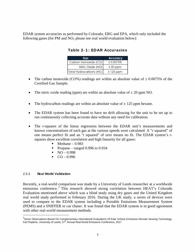
EDAR system accuracies as performed by Colorado, ERG and EPA, which only included the following gases (for PM and NO2 please see real world evaluation below):

Table 2-1: EDAR Accuracies

• The carbon monoxide (CO%) readings are within an absolute value of ± 0.0075% of the

Certified Gas Sample.

• The nitric oxide reading (ppm) are within an absolute value of ± 20 ppm NO.

• The hydrocarbon readings are within an absolute value of ± 125 ppm hexane.

• The EDAR system has been found to have no drift allowing for the unit to be set up to

run continuously collecting accurate data without any need for calibration.

• The r-squares of the linear regression between the EDAR unit’s measurements and known concentrations of each gas at the various speeds were calculated. A “r squared” of one means perfect fit and an "r squared" of zero means no fit. The EDAR system’s r-squares show excellent correlation and high linearity for all gases:

Methane – 0.983 Propane – ranged 0.996 to 0.934 NO – 0.998 CO – 0.996

2.3.3 Real World Validation

Recently, a real-world comparison was made by a University of Leeds researcher at a worldwide emissions conference. 2 This research showed strong correlation between HEAT’s Colorado Evaluation mentioned above which was a blind study using dry gases and the United Kingdom real world study performed in February 2016. During the UK study, a series of devices were used to compare to the EDAR system including a Portable Emissions Measurement System (PEMS) and a SNIFFER or car chaser. It was found that the EDAR system is in good agreement with other real-world measurement methods. 2Some Observations Based On Complementary International Evaluations Of Edar Vehicle Emissions Remote Sensing Technology, Karl Ropkins, University of Leeds, 27th Annual Real World Emissions Conference, 2017

8

The controlled gas study and the “real-world” comparisons are feature in a peer review journal article Evaluation of EDAR vehicle emissions remote sensing technology3

Figure 2-3: Illustration of PEMS Vehicle as Seen in Ropkins Presentation

Figure 2-4: Illustration of SNIFFER (Car Chaser) Vehicle as Seen in

Ropkins Presentation

Table 2-2: R2 Agreements in UK Study as Seen in Ropkins Presentation

Gas

R2 Agreement

with PEMS

Figure 2-5: EDAR and PEMS Correlation in UK Study as Seen in

Ropkins Presentation

3 K. Ropkins et al. / Science of the Total Environment 609 (2017) 1464–1474

9

Photos from Ropkins presentation cited in footnote.

2.3.4 Speed and Acceleration

The vehicle speed measurement is recorded to within ± 1.0 miles per hour. The vehicle acceleration measurement is recorded to within ± 0.5 miles per hour per 1.0 second.

2.3.5 Calibrations and Audits

EDAR’s temporary deployment system was used in Scotland with one EDAR unit that was deployed using specially designed transportable truss system. For this study, HEAT deployed the EDAR system for a week at a time at two separate locations in the Edinburgh and Broxburn areas. Each session during the study was monitored remotely via the Internet for correct operation and data collection. As noted earlier, the nature of the EDAR unit's technology eliminates the need for field calibration. The EDAR system’s patented technology uses similar principals as active satellite remote sensing platforms that constantly subtracts out the background. Due to the absolute nature of the EDAR unit’s measurement techniques, it can remotely measure quantities and relative amounts of targeted pollutants in an exhaust plume without the need for calibration. This gives HEAT’s data unprecedented accuracy, precision and consistency, and allows for minimal human operational intervention. In spite of the inherent stability and accuracy of EDAR technology, HEAT conducts quality assurance tests before and after each project to document for the client whether the EDAR system’s performance has significantly changed during shipping or during the testing deployment. The QA test compares the output of the EDAR system to the known ratios of NO and NO2 calibration gases mixed with CO2. These calibration gases are sourced from well-known specialty gas providers and are produced to U.S EPA standards. The gas values are all accurate to within 1% of the stated concentration ratios and are traceable to the National Institute of Standards and Technology. So, it is certain if the EDAR system’s output does not match the ratio on the calibration gas cylinder, the EDAR system’s output is incorrect and it must be repaired. The QA test is repeated 10-times before shipping to the project location and 10-times after receiving the EDAR unit back from the project. The column plots in Figure 2-6 show the results of the QA test comparisons for this project. Results for the NO calibration gas bottle are in the blue columns on the left, with the light blue being the EDAR unit’s output and the error bars at the top of the column showing the 95% confidence interval for the average. Results for the NO2 calibration gas bottle are in the same format on the right side of the figure, but using a green colouring. In all cases, the average

10

output of the EDAR unit was within 1% of the known calibration gas cylinder values, proving that the EDAR system’s accuracy was not affected by shipping or deployment to Scotland.

Figure 2-6: EDAR QA Test Results Before & After This Pilot Project

Before Project After ProjectCal. Gas Ratio 0.006798 0.00337EDAR output 0.006825 0.003341

0.0000

0.0010

0.0020

0.0030

0.0040

0.0050

0.0060

0.0070

0.0080

0.0090

EDAR QA Tests: NO/CO2 Ratio

Before Project After ProjectCal. Gas Ratio 0.003936 0.003331EDAR output 0.00388 0.003339

0.0000

0.0005

0.0010

0.0015

0.0020

0.0025

0.0030

0.0035

0.0040

0.0045

EDAR QA Tests: NO2/CO2 Ratio

2.3.6 Screening of Hourly Data

HEAT’s EDAR units were monitored remotely in Scotland. Parameters were set up so that HEAT’s engineers would be alerted to anomalies or changes that did not meet HEAT’s specifications for field operations. There were no known issues during this pilot.

2.4 Analysis of Collected Data

HEAT applied the following screening checks to the measurements to ensure the data used for fleet evaluation and fleet comparisons were reasonable and consistent:

o Screening of exhaust plumes o Screening for Vehicle Specific Power (VSP) range

These screening procedures are described in the following paragraphs. The VSP screening is described in section 2.4.2

2.4.1 Screening of Exhaust Plumes

Since the EDAR system measures the exhaust plume with a sheet of laser light scanning across the roadway, the EDAR system is able to construct two-dimensional images of passing vehicles and their respective emission plumes. One axis of the image depicts the length across the road, while the other axis depicts the passage of time. The EDAR system can form a 2D passive infrared image of a vehicle as the vehicle moves underneath the unit. The vehicle image can show the shape of the vehicle, its lane position and the position of its tailpipe. In addition, the EDAR system forms an active image of a vehicle’s emission plume showing the quantity of

11

pollutant detected per unit area or optical mass in moles/m2. The plume image shows the position of the plume for each pollutant as well as the dispersion rate of the plume. The gas record is considered valid if there is one scan where the average measurement of CO2 in the scan exceeds 0.004 moles/m2. Furthermore, the linear correlation coefficient or Pearson’s correlation criteria (r) is applied between the CO2 measurements and the CO, NO and NO2 measurements. If the correlation factor is relatively high, the measurement is considered valid. This signifies that there are no interfering plumes. Interfering plumes usually have different ratios of pollutant to CO2; therefore, the linear correlation coefficient drops in value. The highest linear correlation coefficient is 1.0, whereas values near zero indicate no correlation and negative 1.0 indicates complete negative correlation. When gas readings are near zero for CO, NO and NO2, then correlation values are ignored, because of the lack of presence of those gases

Figure 2-7: Vehicle Driving Through the Plume of a Preceding High Emitter

12

2.4.2 Vehicle Specific Power

In order to make meaningful comparisons between various vehicle emissions testing methodologies, it is important to know the instantaneous loading conditions of the vehicle under test. This is particularly true for the case of remote sensing measurements, where a “snapshot” of the emissions of the vehicle under test is captured at a specific loading condition. In 19994, Jimenez advanced a new metric called Vehicle Specific Power (VSP) as a development over prior load classification parameters. VSP is an estimate of the ratio of instantaneous vehicle power to vehicle mass. The main advantage of VSP is that it avoids the necessity of knowing intrinsic vehicle and engine parameters in favour of parameters that can mostly be acquired remotely, like vehicle speed/acceleration and road grade. It is also advantageous in its simplicity as being a one-dimensional parameter. Jimenez showed the effectiveness of VSP through comparative analysis and was later adopted by the EPA for use in its modelling efforts5. The equation for VSP incorporates various loading components acting on the vehicle under test. It includes the internal effect of “acceleration resistance,” due to the engine’s rotating components, as well as the external effects of road grade, rolling resistance, and aerodynamic drag. Jimenez developed typical values for each effect which are embedded in the following equation:

4 Cires.colorado.edu/jimenez/Papers/Jimenez_PhD_Thesis.pdf 5 www.epa.gov/ttnchie1/conference/ei12/mobile/koupal.pdf

Where:

is specific power in , , or

is vehicle speed in

is vehicle acceleration in is roadway angle of inclination to the horizontal

i h d i d d i

13

In summary, the main use of VSP in remote sensing is for screening out vehicles which could be under high load and operating open loop (not near stoichiometry, or in this case a point at which all of the oxygen and fuel has been consumed, and therefore are expected to have high emissions) or at very low load where the vehicle would not produce NO or NO2 because the vehicle is not under load.

2.5 Sources of Data and Data Collected

The EDAR unit pollutant measurements (CO2, NO, NO2, & PM2.5) and the ANPR were the two main sources of data used for this report. The information below demonstrates the format of the data collected in this report.

2.5.1 Information Collected

o HEAT units operated – EDAR 7 o Date o Time o License plate image o CO2, NO, NO2, & PM2.5 measurements o Speed o Acceleration o Temperature of the exhaust

2.5.2 Data Collection Statistics

o Unit o Site o Date o Time o Hourly temperature o Hourly humidity

2.5.3 Vehicle Registration Data

The license plate data collected by the HEAT license plate recognition camera system was submitted to CDL Vehicle Information Services Limited, so that vehicle VIN and other vehicle data could be provided for analysis. The information provided includes:

o License plate o Euro Class o Model year o Make o Body style o Engine Size o Fuel Type o Vehicle Type

15

3 STUDY DESIGN

3.1 Deployment Method

HEAT performed a two-week deployment in March of 2017 to collect on road real world emissions data from Scottish vehicles to determine the contribution of pollutants from in use vehicles using its unmanned, unobtrusive EDAR Emissions Camera. The EDAR system was installed in two separate locations in the Edinburgh and West Lothian areas utilizing a specially designed truss system, which was evaluated for safety and wind resistance and then secured to a one-ton concrete base. This truss system is over engineered for safety and precision as well as ease of deployment. The specially designed truss was equipped with an electrical arm for ease of securing the EDAR system. The expert local civil engineering firm Lochwynd, which specializes in traffic and roadwork, was contracted by HEAT to assist with the coordination of the installation. Safety of the engineers and motorists is of utmost importance to HEAT in the installation of the EDAR unit and its components. In addition to the EDAR unit, an ANPR, speed and acceleration unit, weather sensor, electrical panel, and retroreflector are all installed as part of a complete EDAR system. The two-inch-wide retroreflector was installed in the roadway in a similar fashion as traffic signal loops. This unobtrusive reflector allows for operations in light rain or misty conditions, which allows for increased up time.

Figure 3-1: Truss System Deployed On Road

Figure 3-2: Drawing of Truss System

16

3.2 Measurement Sites

Working closely with the East Central Scotland Vehicle Emission Partnership, who liaised with Local Authorities, and wider stakeholders (including Transport Scotland) a range of possible locations for the pilot measurement were reviewed using the following criteria. Location Criteria

• Provide a representative sample of the various parts of the Scottish fleet (cars, buses, taxis, freight), and of differing road types.

• Maximise the total number of vehicles measured. • Choose locations with a slight gradient to ensure the vehicles were operating under load. • Include different types of road, with ns such as e.g. Barriers). Data collection and pilot criteria.

• Support the work of the East Central Scotland Vehicle Emissions Partnerships in identifying high polluters on emissions.

• Gather fleet emission data to add value to the National Modelling Framework (NMF, described in CAFS).

• Consider the use of instantaneous vehicle emission data in LEZ awareness raising and enforcement (linked to ANPR, and assessment of high polluters).

From all of the above the pilot team agreed two sites in the City of Edinburgh, and West Lothian. Table 3-1 below provides the details about each site including the exact location coordinates.

Table 3-1: Description of Sites where Sampling was Performed

Figure 3-3 shows the locations on a map.

17

Figure 3-3: Location of Sampling Sites (marked in yellow)

18

3.3 Weather Considerations

Inclement weather such as rain or heavy snow resulting in wet pavement prevents remote sensing devices from taking accurate reads due to the fact that water is a large absorber of infrared light. However, due to advances made with the EDAR system, the unit was able to continue taking data in mist and light rain. In addition, fog, dust, humidity, mist or light rain does not affect the measurement of the EDAR system’s reads of gasses. Tables 3-2 to 3-7 show the weather conditions during the deployment.

Table 3-2: Edinburgh Weather Conditions

Table 3-3: Broxburn Weather Conditions

19

Table 3-4: Edinburgh Temperature (°C)

Table 3-5: Broxburn Temperature (°C)

20

Table 3-6: Edinburgh Humidity (%)

Table 3-7: Broxburn Humidity (%)

21

3.4 Intelligent Reflector

Once the EDAR unit is deployed on the transportable gantry, as shown in Figures 3-1 and 3-2, the operator aligns the unit to scan to the in-road reflector used to enhance surface albedo. This bespoke reflector (used for the first time in the Scotland pilot) was designed to improve the EDAR unit performance in conditions of mist and light rain. The reflector is deployed by securing and sealing it into a narrow transverse channel cut in the carriageway (in a similar manner to traffic sensor loops). When placed in position it is hidden and undetectable to road users. The reflector significantly increased data capture during light rain and mist due to increased albedo, and after heavy rain due to the reduction of spray from tires during the surface drying period. For example, on 29th March 2017, there were intermittent rain showers throughout the day beginning at 12:00 and continuing until nearly 16:00. When analysing the EDAR valid gas data (Table 3-8 and Figure 3-4), it can be seen that in between rain showers EDAR was able to begin collecting valid data again very quickly (most instances showed very small gaps in time usually only lasting a few minutes).

Table 3-8: Sample Weather Data from 29 March 2017

22

Figure 3-4 shows the brief downtime experienced during a rain event. In previous operations, the period during a rain event would have not resulted in any data points, but with the EDAR system’s advanced reflector the four-hour rain event only amounted to one hour of downtime due to the reflector’s drying capabilities.

Figure 3-4: EDAR Data During a Rain Event

23

4 ANALYSIS OF DATA COLLECTED

4.1 General Statistics

The data was collected continuously over thirteen days in March using EDAR 7. A total of 81,240 attempted measures were made. Of those, 5,615 vehicles were excluded due to interfering plumes, 947 had unreadable plates, and 362 vehicles were from other countries resulting in a sample of 74,316 vehicles. The 74,316 were sent to CDL out of which registration data matched 70,318. Table 4-1 below shows the EDAR system’s measurements made during the period of testing in Edinburgh and Broxburn. Vehicles registered in other countries comprised 0.44% of the survey.

Table 4-1: EDAR Data Statistics

24

Figure 4-1: EDAR Data Statistics in Bar Chart Format

The overall daily attempted and valid reads by location are shown in Table 4-2. The overall valid hit rate was 91 percent despite the adverse weather conditions over the two-week period.

Table 4-2: Daily Valid and Attempted Measures

25

Figure 4-2: Daily Valid and Attempted Measure Bar Chart

Table 4-2 summarizes how many vehicles of each type, fuel, and Euro class had their emissions measured at each site. These observations are for valid EDAR measurements of all vehicles, under any driving condition prior to being filtered for exhaust temperature or VSP. By presenting all accurately measured vehicles, this table demonstrates the full number and type of vehicles that are possible to measure at these sites and over the project time-span of thirteen (13) days.

As expected, the vast majority of vehicles passing the two measurement sites were diesel or petrol fuelled cars. Out of about 70,000 vehicles properly measured, almost 60,000 (85%) of them fell into these two categories. The next two largest vehicle categories were vans and Ordinary Goods Vehicles (OGV), which are almost entirely fuelled by diesel. Additionally, taxis and buses are a significant proportion of the observed fleet and are also mostly fuelled by diesel.

26

The Euro classification of the fleet is highly skewed to the latest three standards, Euro 4, 5 and 6 -- especially for the car category. The most frequently observed classification for cars was Euro 5, with Euro 4 and 6 combining to almost equal the Euro 5 car observations. Interestingly, the OGV portion of the fleet was skewed even more toward the Euro 5 and 6 classes. Except for the OGV portion, the commercial portion of the fleet is less skewed to the modern classes than the cars.

Table 4-3: Number of Vehicles Measured by Vehicle Type and Fuel Type

27

Table 4-4: Observed Vehicle Types and Proportions at the Pilot

Locations

The Euro classifications are also represented at approximately the same ratios at the two measurement sites. Euro 5 vehicles totalled slightly less than half of all observations at each of the sites. Vehicles of the Euro 4 or Euro 6 class were observed in about the same proportions, and at about half the frequency of Euro 5 vehicles. The latest three Euro classes (4,5 and 6) combined to represent almost 64,000 out of the 70,000 vehicles measured by the EDAR system at both sites.

28

Table 4-5: Distribution of Fuel Type and Euro Class by Location

Figure 4-3: Broxburn Number of Vehicles by Fuel Type and Euro Class Bar Chart

Figure 4-4: Edinburgh Number of Vehicles by Fuel Type and Euro Class Bar Chart

29

Figures 4-5 through 4-9 are stacked-column charts showing the proportions of the sub-fleets measured by the EDAR unit that fall into each Euro class for cars, OGVs (ordinary goods vehicles) and buses. In general, cars are light duty vehicles not used for commercial purposes, OGVs are medium and heavy-duty commercial vehicles for transporting goods and services and buses are commercial vehicles used to transport persons that are not registered as taxis. When appropriate, the prevalence of each fuel type is also indicated in the charts through the differing colours that comprise each column. The chart in Figure 4-5 is for the car sub-fleet. In the older Euro classes, the proportion of petrol cars was dominant over that of diesel cars. However, in the more recent Euro classes (5 and 6), diesel cars have come to represent about half of each category. By adding the proportions of fuels in each category one can determine that overall, diesels are 44% of the car fleet and petrols are 56%.

Figure 4-5: Observed Car Fleet by Euro Class & Fuel

30

The chart in Figure 4-6 is for the OGV sub-fleet. One can immediately see that the OGV sub-fleet measured by the EDAR unit was entirely fuelled by diesel. Another notable feature of the OGV vehicle fleet is that it is quite young, with 77% conforming to either the Euro 5 or Euro 6 classification. This increase could be due to the need for home delivery services and online shopping.

Figure 4-6: Observed OGV Fleet by Euro Class & Fuel

31

Figure 4-7 is a chart for the Bus sub-fleet. The buses are not quite as young as the OGV sub-fleet, with a bit more than 76% being spread over Euro 4, Euro 5 and Euro 6 in approximately equal proportions. Another difference with the OGV group is that a few buses are fuelled by petrol, such as 11 seat minibuses.

Figure 4-7: Observed Bus Fleet by Euro Class & Fuel

32

Figure 4-8 shows that the taxi fleet is entirely fuelled by diesel and is dominated by the Euro 5 class (400 Euro 5 out of 704 total taxis). Figure 4-9 shows that the fleet of vans has an age distribution similar to that of taxis with the exception that a smaller proportion of vans are in the older Euro 0-2 classes.

Figure 4-8: Observed Taxi Fleet by Euro Class & Fuel

Figure 4-9: Observed Van Fleet by Euro Class & Fuel

33

4.2 Speed

The plots in Figures 4-10 and 4-11 are histograms showing the distribution of the speeds of vehicles at the two measurement sites. The Broxburn site had a total of 29,238 measurements and the Edinburgh site total was 41,080. The sites had significantly different speed distributions, with Broxburn having more vehicles traveling at a wider range of speeds around its modal bin of 24 mi/hr and the Edinburgh vehicle speeds being more tightly concentrated around its modal bin of 28 mi/hr. The reason the Broxburn site had vehicles traveling over a wider range of speeds than the Edinburgh site is most likely due to the higher congestion at the Edinburgh site. The Broxburn site traffic was more free-flowing due to a traffic light being located just “upstream” of the measurement site.

Figure 4-10: Broxburn Speed

3 1 14355

3562

70157374

4118

24012227

1339

593

154 63 13 4 20

1000

2000

3000

4000

5000

6000

7000

8000

0 4 8 12 16 20 24 28 32 36 40 44 48 52 56 60 64

Coun

ts

Speed Bin (mi/hr)

Broxburn Speed Histogram

Figure 4-11: Edinburgh Speed

12 6 17 37 169

1167

7966

17053

9758

3482

1089235 54 22 10 1 2

0

2000

4000

6000

8000

10000

12000

14000

16000

18000

0 4 8 12 16 20 24 28 32 36 40 44 48 52 56 60 64

Coun

ts

Speed Bins (mi/hr)

Edinburgh Speed Histogram

4.3 Vehicle Fleet Emission Statistics

The overall emissions results are presented in this section. In these results, the gaseous pollutants are expressed in two ways. They are either in terms of their concentration relative to the concentration of CO2 in the exhaust or they are in terms of their mass in relation to the mass of fuel combusted to produce the exhaust. When the molar concentration ratio is used, the units are moles of pollutant per mole of CO2, or mole/mole. This can be thought of as a molecular concentration. For example, a NO concentration of 0.001 moles/mole would mean that for every 1,000 molecules of CO2 in the exhaust, 1 molecule of NO is also present (i.e., 1/1000 = 0.001). When the mass concentration is used, the units are grams of pollutant per kilogram of fuel, or g/kg. For example, a NO result of 1 g/kg means that for every 1,000 grams (i.e., 1 kilogram) of fuel used by the engine, 1 gram of NO is also emitted.

34

A calculation of grams of pollutant/kg of fuel is used because it requires no assumption about the fuel density as opposed to using g/litre of fuel. Expressing pollutants in this way allows for the straightforward estimation of emissions inventories based upon the fuel consumption of the fleet. PM is expressed a bit differently than the gaseous pollutants. The PM measurement can be thought of as the number of PM particles as compared to the number of CO2 molecules in the exhaust. So, a PM concentration of 1.0 nmoles/mole would mean that for every 1-billion molecules of CO2 in the exhaust, 1 particle of PM would also be present (i.e., 1/1,000,000,000 = 0.000000001 moles = 1.0 nmole).

4.3.1 Edinburgh and Broxburn Average Emissions by Euro Class and Major Fuel Type

Figures 4-12 through 4-14 show plots of fleet-average pollutant concentrations for each Euro Class and major fuel (petrol or diesel). In this case, the “fleet-average” groupings include all types of vehicles that used the specified fuel and conformed to the specified Euro standard. (Note that the Euro 0, Euro 1 and Euro 2 vehicles have been combined into a category named Euro 0-2 because these three classes comprise a small fraction of the fleet.) The concentrations are expressed as moles of pollutant per mole of CO2 in the exhaust. In the case of particulates, particles are measured instead of molecules, so the results for PM should be thought of as nanomoles of PM particles per mole of CO2 molecules in the exhaust. Figure 4-12 shows the average NO emissions for the fleet for each Euro Class category. The diesel vehicle groups on average do not show a reduction in overall NO across the Euro classes. Although the Euro 6 class has a lower average of NO emissions, the levels of NO remain relatively high, being only half or more of the previous Euro classes. Unlike the diesels, the petrol fuelled vehicles showed a strong decrease in average NO emissions with each successive Euro Class. These trends were expected since petrol vehicles have controlled NO emissions with the widespread use of three-way catalysts since the mid-1990s, but diesel vehicles only began the widespread use of catalysts for NO reduction more recently (beginning with the Euro 6 standards for heavy-duty and with the Euro 4 for light-duty).

35

Figure 4-12: Average NO/CO2 Ratio by Fuel and Euro Class

Figure 4-13 shows the average NO2 emissions for the fleet. In this case, the diesel groups show a somewhat increased level of NO2 emissions in the middle Euro groups whereas the petrol groups show a sharp decrease Euro 0-2 to Euro 3 and for the younger euro class (Euro 6). Notice that the diesel Euro 3 through 6 class levels all are higher than the Euro 0-2 class group.

Figure 4-13: Average NO2/CO2 Ratio by Fuel and Euro Class

36

Figure 4-14 demonstrates the results for PM emissions. In this case, the petrol vehicles show no significant trend with Euro Class but the diesels show a generally higher average for the older diesel Euro groups (0 through 4) and a lower average for the newer Euro groups (5 and 6).

Figure 4-14: Average PM2.5/CO2 Ratio by Fuel and Euro Class

4.3.2 Edinburgh and Broxburn Average Emissions by Euro Class, Fuel and Vehicle Category

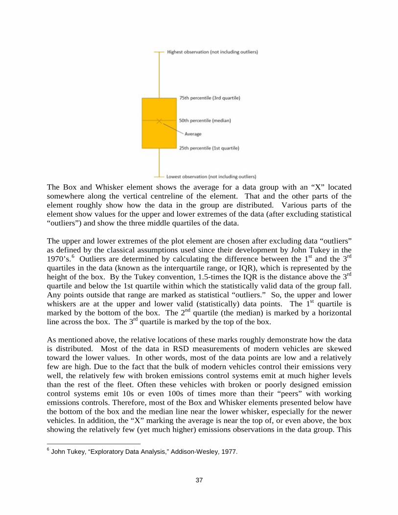
The following series of plots summarize the emissions results from the vehicle types listed below, for the Euro class for the major fuels used in each category: Car (petrol and diesel), OGV (ordinary goods vehicle) (diesel only), Bus (diesel only), Taxi (diesel only) & Van (diesel only). Since the fraction of the fleet representing either Euro 0, Euro 1, or Euro 2 vehicles is quite small, all of these vehicle types were combined into a group called Euro 0-2. The Euro 0-2, Euro 3, Euro 4, Euro 5 & Euro 6 class groups are each treated separately in this analysis. To give a better idea of the distribution of emissions within each of these groups, the results are presented using a Box and Whisker analysis. This calculates a representative range of emissions within each group and presents the result graphically using a Box and Whisker plot. The following graphic shows a generic Box and Whisker plot element with labels describing what its various parts represent.

37

The Box and Whisker element shows the average for a data group with an “X” located somewhere along the vertical centreline of the element. That and the other parts of the element roughly show how the data in the group are distributed. Various parts of the element show values for the upper and lower extremes of the data (after excluding statistical “outliers”) and show the three middle quartiles of the data. The upper and lower extremes of the plot element are chosen after excluding data “outliers” as defined by the classical assumptions used since their development by John Tukey in the 1970’s.6 Outliers are determined by calculating the difference between the 1st and the 3rd quartiles in the data (known as the interquartile range, or IQR), which is represented by the height of the box. By the Tukey convention, 1.5-times the IQR is the distance above the 3rd quartile and below the 1st quartile within which the statistically valid data of the group fall. Any points outside that range are marked as statistical “outliers.” So, the upper and lower whiskers are at the upper and lower valid (statistically) data points. The 1st quartile is marked by the bottom of the box. The 2nd quartile (the median) is marked by a horizontal line across the box. The 3rd quartile is marked by the top of the box. As mentioned above, the relative locations of these marks roughly demonstrate how the data is distributed. Most of the data in RSD measurements of modern vehicles are skewed toward the lower values. In other words, most of the data points are low and a relatively few are high. Due to the fact that the bulk of modern vehicles control their emissions very well, the relatively few with broken emissions control systems emit at much higher levels than the rest of the fleet. Often these vehicles with broken or poorly designed emission control systems emit 10s or even 100s of times more than their “peers” with working emissions controls. Therefore, most of the Box and Whisker elements presented below have the bottom of the box and the median line near the lower whisker, especially for the newer vehicles. In addition, the “X” marking the average is near the top of, or even above, the box showing the relatively few (yet much higher) emissions observations in the data group. This

6 John Tukey, “Exploratory Data Analysis,” Addison-Wesley, 1977.

38

greatly influences the result of the group’s calculated average. After being used to calculate the quartiles, median and average of the data group, the observations marked as statistical outliers are not thrown away. For example, the high outliers are typically good candidates for further investigation as vehicles with possibly malfunctioning emissions control systems. Figures 4-15 through 4-20 show six plots for the NO emissions results from each vehicle category and fuel. Figure 4-15, comparing the Euro group results for NO from petrol cars, shows the well-known trend of older vehicle groups having higher average emissions and much larger variability (especially to the high side) than newer groups. As the Euro groups get younger, the emissions averages get much cleaner and less variable.

Figure 4-15: Petrol Cars NO/CO2 Ratio by Euro Class

As shown below, unlike the petrol vehicles the trend for diesel cars is not pronounced until the very newest group, Euro 6. All groups have similar distributions, but the Euro 6 group is cleaner, on average, than the others. Figure 4-16 shows the diesel cars NO distributions for each vehicle class is very similar except for the Euro 6, which is slightly cleaner on average.

39

Figure 4-16: Diesel Cars NO/CO2 Ratio by Euro Class

Figure 4-17 the diesel buses NO results are more mixed, with higher average emissions for the oldest Euro group (0-2) and the Euro 5 group. The Euro 6 group has the cleanest and more skewed emissions of all bus groups.

Figure 4-17: Diesel Buses NO/CO2 Ratio by Euro Class

40

Figure 4-18 shows the trend for OGVs with the Euro classification for NO to be not as classical. Euro class 0-2 on average actually has lower emissions than Euro 4 and 5, but the newest group (Euro 6) has the cleanest average and most skewed distribution of all the OGVs. Figures 4-19 and 4-20 shows Taxis and Vans to be similar to the OGVs in the relative levels of their NO averages for the Euro groups.

Figure 4-18: Diesel OGV NO/CO2 Ratio by Euro Class

Figure 4-19: Diesel Taxis NO/CO2 Ratio by Euro Class

41

Figure 4-20: Diesel Vans NO/CO2 Ratio by Euro Class

Figure 4-21 shows results from petrol cars for NO2. The group-averages trend lower with newer Euro class until Euro 4, from above 0.0002 mole/mole down to about 0.0001 mole/mole. The trend then flattens and emissions remain about the same through Euro 6.

Figure 4-21: Petrol Cars NO2/CO2 Ratio by Euro Class

42

Figures 4-22 – 4-24 demonstrate that for diesel cars, OGVs and vans the middle Euro classes (Euros 3,4, & 5) have higher average emissions than the older and youngest classes (Euros 0-2 & 6). Due to its higher upper quartile and outlier measurements, even the Euro 6 class has a higher average than the Euro 0-2 class group (except for the OGVs).

Figure 4-22: Diesel Cars NO2/CO2 Ratio by Euro Class

Figure 4-23: Diesel Vans NO2/CO2 Ratio by Euro Class

43

Figure 4-24: Diesel OGV NO2/CO2 Ratio by Euro Class

Figures 4-25 and 4-26 demonstrate the NO2 data for buses and taxis. The average NO2 emissions levels actually increase with the youth of the Euro group (Euro 6).

Figure 4-25: Diesel Buses NO2/CO2 Ratio by Euro Class

44

Figure 4-26: Diesel Taxis NO2/CO2 Ratio by Euro Class

For Figures 4-27 through 4-32 the pollutant displayed is PM. In Figure 4-27, Petrol cars stand out from the other vehicle groups in that they show no real trend in PM emissions with age or Euro group. Also, with the petrol cars, the PM distributions are skewed toward the low end. The lowest value, the 1st quartile and the median are all indistinguishable from each other at the bottom of the element for each Euro group, yet the averages are all above the 3rd quartile line (i.e. above the box). This shows how a large majority of observations are at or near zero, while the relatively few high observations more than offset the weight of the low measurements by how high they are compared to the bulk of the group.

45

Figure 4-27: Petrol Cars PM2.5/CO2 Ratio by Euro Class

The diesel vehicle groups show a general trend of increasing average PM emissions as vehicles get older (i.e., the stricter the standard the lower the emissions). There are minor exceptions in the Taxi and Bus groups, in that the middle groups (Euro 3, 4 & 5) appear a bit higher on average.

Figure 4-28: Diesel Cars PM2.5/CO2 Ratio by Euro Class

46

Figure 4-29: Diesel Buses PM2.5/CO2 Ratio by Euro Class

Figure 4-30: Diesel Taxis PM2.5/CO2 Ratio by Euro Class

47

In Figure 4-31, diesel vans show a decrease in PM for Euros 5 and 6.

Figure 4-31: Diesel Vans PM2.5/CO2 Ratio by Euro Class

Figure 4-32 demonstrates that OGVs have a slight uptick in PM numbers for the Euro 6 class. The distribution of the results for Euro 6 are greatly skewed toward the low end, nearer to zero. This indicates that most Euro 6 OGVs emit lower than the other Euro classes, but the few, relatively high “outliers” are bringing the average result a bit higher than for Euro 4 and 5.

Figure 4-32: Diesel OGV PM2.5/CO2 Ratio by Euro Class

48

4.3.3 Approximate Emission Contributions by Model Year

The sampled population distribution and average emissions concentrations by model year are shown in Figures 4-33 to 4-36. In these figures, the overall emission ratios for the entire fleet per year of manufacture since 2000 is calculated to give a global view of the fleet for both petrol and diesel vehicles. This includes all vehicle types except for motorcycles. Figure 4-33 shows the distribution of sample sizes for each model year and fuel. The sample sizes for each model year for the early years of the 2000’s is proportionally higher for petrol vehicles, showing that the diesel fleet is somewhat younger than the petrol fleet at these two sites. As shown by the approximately same total areas of the petrol and the diesel columns, the petrol and diesel fleets are very nearly the same size overall.

Figure 4-33: Edinburgh and Broxburn Vehicle Totals by Model Year Diesel vs Petrol

Model Year

Range Euro Class

2000-2004 Euro 3 2005-2008 Euro 4 2009-2013 Euro 5 2014-2017 Euro 6

49

Figure 4-34 has a column chart showing the average NO emissions for each model year since 2000 from the diesel and petrol vehicles. For diesel, there is a rise in NO as Euro 5 vehicles enter the fleet at approximately the 2008 models, then a drop is seen as Euro 6 models enter the fleet at around 2014. The NO for petrol vehicles is flat from 2008 and higher. The ageing and deterioration of NO emissions control measures are most likely the reason for the higher NO for petrol vehicles from 2007 and older along with the diesel vehicles. The air quality impacts of these higher emissions from older vehicles is somewhat lowered by the fact that they represent a fairly small fraction of the on-road fleet.

Figure 4-34: Edinburgh and Broxburn Average NO Emissions (moles/mole CO2) by Model Year

Model Year

Range Euro Class


50

Figure 4-35 shows that on average, NO2 is lower for older diesels than for the younger diesels. This could be due to the new oxidation catalysts that were more prevalently employed from 2005 and higher. The SCR NOx mitigation system in Euro 6 class could be the reason for the drop in NO2 from 2014 on. Overall, the NO and NO2 plots show that the majority of the NOx is from the diesel vehicles, as expected. This is made more likely because diesel vehicles tend to have higher annual mileage than petrol vehicles.

Figure 4-35: Edinburgh and Broxburn Average NO2 Emissions (moles/mole CO2) by Model Year

Model Year

Range Euro Class


51

In Figure 4-36, the PM per model year averages show how from 2000 to 2009 the diesel cars had much higher PM number emissions than the petrol. A change occurred at about 2012 and now the petrol fleet has higher average PM number emissions. It is speculated that this is could be due to the more fuel-efficient direct-injection systems that have become more and more prevalent in the newer petrol fleet.7 Figure 4-36: Edinburgh and Broxburn Average PM2.5 Emissions Ratio

(nmole/mole) CO2 by Model Year

Model Year Range

Euro Class


7 Archer, Greg, Briefing: Particle emissions from petrol cars, Transport and Environment, November 2013, Brussels

52

4.4 Unique Capabilities

The EDAR system has several capabilities that other vehicle remote sensing systems cannot match. Several of these capabilities are highlighted in this section through descriptions and analysis. To add context to the later descriptions, the Euro Standards are reviewed first.

4.4.1 Euro Standards

Vehicles entering a Low Emission Zone (LEZ) are expected to meet a certain emission rate per Euro Standard based on the vehicle fuel type and size. These rates are outlined in Table 4-6, which were instated in 1992, when the Euro 1 Standard was introduced. The standards now go through Euro 6 for light duty and Euro VI for heavy duty. These standards were taken into consideration when performing the analysis of on the on-road emissions testing for this pilot. Table 4-6: Required Emissions Limits and Euro Standard by Vehicle

Type

53

Source: UK National Atmospheric Emissions Inventory (NAEI)

4.4.2 Grams per Kilometre

One of the EDAR system’s unique capabilities is to directly measure the mass of pollutants per distance of vehicle travel (e.g., g/km) by measuring the absolute amount of pollutants left behind as the vehicle passes. The EDAR system quantifies the plume as it disperses behind the vehicle. Therefore, the EDAR system calculates the total amount the vehicle leaves behind as long as the total plume is in the field of view. The length of the field of view is accurately known, so the grams/distance can be directly calculated from the EDAR unit’s data. Because of this capability, EDAR can produce measurements that are directly comparable to the new vehicle emissions standards in Europe. However, some post processing is necessary because the EDAR unit’s measurements are not typically taken under conditions that mimic the laboratory tests required by the Euro standards. This is briefly discussed in the next two paragraphs. The grams per kilometre (g/km) is a unit used to express the European emission standards (harmful emissions classifications). Vehicle manufacturers must prove their vehicles conform to these standards before they are allowed to sell them in the European market. The standards are set by measuring the amount of pollutants emitted by vehicles on a chassis dynamometer using the New European Drive Cycle (NEDC) in the controlled conditions of a laboratory. The NEDC procedures have many stops, negative accelerations, and positive accelerations; therefore, large variations in VSPs. It is well known that the higher the load on the engine (which is proportional to VSP) the higher the NOx emitted by the engine. (In properly functioning vehicles, the “engine-out” emissions levels are greatly reduced by a pollution control system before being emitted from the vehicle’s exhaust pipe.) As mentioned, the EDAR unit usually measures exhaust from vehicles that are operating at a higher VSP than the average for the NEDC. Thus, the instantaneous g/km detected by the EDAR unit will be larger on average than for the same vehicle tested on the NEDC. HEAT has developed algorithms to compensate for this by scaling the EDAR CO2 g/km so that the adjusted EDAR CO2 g/km matches the average CO2 g/km ratings from the car manufactures. The EDAR unit’s pollutant results are scaled accordingly for each time a vehicle

https://www.ngk.de/en/technology-in-detail/lambda-sensors/basic-exhaust-principles/exhaust-and-harmful-emissions/

54

is measured to compensate for the bias between the VSP of the EDAR measurement and the VSP of the NEDC. The results from this pilot’s diesel cars (since they are the most prevalent vehicle type in the fleet) are described below. Column plots show the average emissions levels for each model year. Figure 4-37 shows the scaled NO g/km results from the EDAR system for the Edinburgh and Broxburn sites. The higher averages from 2000-2001 are most likely due to the higher age of those vehicles. For younger vehicles, the NO levels drop until 2007, which is when Euro 4 vehicles start to populate the fleet. As Euro 4 vehicles enter the fleet, NO levels rise possibly indicating a systemic problem with NOx control systems in the Euro 4 and Euro 5 fleets. NO levels have a distinct plateau from 2011- 2014 until Euro 6 vehicles begin to enter the fleet in 2015.

Figure 4-37: Average NO gram/km

55

Figure 4-38 shows the non-classic trend for NO2, with the older vehicles having lower emissions than the newer Euro classes. There is a sharp rise in NO2 as Euro 4 vehicles enter the fleet. This is possibly due to a prevalence of oxidation catalysts (to help PM reduction), oxidizing the NO. Finally, as Euro 6 vehicles enter the fleet, NO2 levels drop again.

Figure 4-38: Average NO2 gram/km

56

Figure 4-39 shows NOx averages (which, for comparison to the standards, is the addition of NO with NO2 using the molecular weight of NO2 for NO, since this is how the Euro emissions standards are defined). By comparison to the previous two figures, it can be seen that the NO is still the dominant species, but the larger relative NO2 from 2005 model years and on give a NOx levels for newer car models the same relative values as much older vehicles. In this data, we see that even with the larger NO2 amounts in the years 2015-2017 the NOx trends down as Euro 6 models enter the market.

Figure 4-39: Average NOx gram/km

57

Figure 4-40 has a column chart showing the average PM results, by model year. The PM measurements have a more classical profile as model year increases, with older vehicles having higher averages than younger ones. This is most likely due to the success of the Euro 4 and 5 standards at forcing technologies that were effective at reducing PM, but as seen above, not effective for NOx.

Figure 4-40: Average PM2.5 nmole/km

58

4.4.3 NOx Emissions per Vehicle Make and Class

Figure 4-41 compares the average NOx emissions from various vehicle makers versus EU standards for NOx. The comparison was performed on makes of light-duty vehicle (cars, vans and taxis) most seen by EDAR. All the makes in Figure 4-41 are seen more than 600 times over a two-week period which allows for a good statistical representation. Since a comparison to emissions standards is being made, the results for NOx are not a simple addition of NO + NO2. By convention, NOx emissions standards are expressed on a “NO2-equivalent” basis. For these plots, NO results are also converted to a “NO2-equivalent” before being added to the NO2 results. In other words, in calculating the mass of pollutants for NOx, the molecules of NO are treated as if they were NO2 instead. Figure 4-41 demonstrates how the results of this analysis are consistent with other, independent studies of in-use emissions8. One would expect that if the vast majority of on-road vehicles have emissions below the Euro standards, their average on-road emissions should at least be comparable (i.e., close to) the standard. Unfortunately, that is not the finding of these results. None of the manufacturer averages for Euro 5 or 6 vehicles were even near-to the Euro 5 or 6 standards for NOx

9. In addition, the largest average, out of the four Euro classes, was Euro 5 for 13 out of the 21 makes analysed (which is more than half of the total manufacturers analysed). This seems to be consistent with the results seen for all manufacturers in this study. Mazda and Ford Euro 3 vehicles had the lowest averages of all their Euro classes. This makes sense because Mazda and Ford share many vehicle platforms. On the other hand, Audi had the highest combined averages for all the Euro classes while Toyota had the lowest. Only one make, Audi, had the classical trend of the older the vehicle, the higher the average is for NOx.

8 Vicente Franco, Francisco Posada Sánchez, John German, and Peter Mock. “Real-world exhaust emissions from modern diesel cars.” Report by International Council on Clean Transportation, October 11, 2014. 9 This is not shown in the graphic, but not even the cleanest 25% of the on-road measurements from the Euro 5 and Euro 6 vehicles measured by EDAR met the Euro 5 or Euro 6 standards.

59

Figure 4-41: NOx Emissions by Make and Euro Class for Diesel Cars

60

4.5 Analysis of Exhaust Temperature Data

Since the EDAR unit has the ability to measure the temperature of the exhaust plume near the exit of the tailpipe, it is possible to determine whether the vehicle engine and exhaust after treatment system are warm. When the exhaust exiting the tailpipe is warmer than the ambient temperature, one can safely assume that not only are the engine and the exhaust pollution control system warm, but the entire exhaust system is also warm. Under this assumption, the number of vehicles in the EDAR system database that did not yet have a fully-warmed exhaust system was determined. Only the vehicle type/fuel combinations with enough samples for a statistically valid comparison were included. Table 4-7 summarizes how many of the vehicles were not yet fully warm when they were measured by the EDAR system.

Table 4-7: Temperature Data for All Vehicles Measured

The diesel fuelled commercial delivery vehicles (diesel van and OGV) seem to have a consistently higher incidence of operating while not fully warm than the other vehicles. It is plausible that these vehicles idle more than other vehicles, due to the higher prevalence of delivery and commercial service for medium and heavy diesels. If that is the case, their exhaust temperature would tend to be cooler during a higher fraction of operations than for other vehicles. To test the assumption that vehicles with catalysts would warm their exhaust systems more quickly than those without catalyst, this same analysis was also performed only for vehicles that likely have catalyst systems as part of their emissions controls (such as three-way catalysts for petrol and SCR for diesel). There were no significant differences in the “catalyst-only” results when compared to the above results. This indicates that the exhaust systems with catalysts are warmed up at about the same rate as those without catalysts.

4.6 Single Vehicle Analyses Using Repeated Measurements

Vehicle remote sensing is well-known as a tool for understanding fleet-wide, in-use emissions. But when properly deployed in an ongoing monitoring program, the EDAR system can also be used to identify individual vehicles and even vehicle models with emissions problems. When a system is easily deployable and unmanned, as the EDAR system is, the number of vehicles receiving multiple measurements can be maximized. As the number of these repeatedly

61

measured vehicles increases, the EDAR unit’s data becomes more and more useful for determining which vehicles exhibit patterns of high, in-use emissions. In this section, the utility of using the statistical power of repeat EDAR measurements on a given vehicle is discussed. Understanding the power of repeat measurements for finding malfunctioning or poorly-designed vehicles is important to understanding the utility of an on-going monitoring program based upon the EDAR system. The steps of the analysis are to first identify which vehicles might have a problem, then to isolate those vehicles for further analysis using their repeat measurements. Historically, it is known that when the EDAR system measures a large and representative sample of the fleet, the similar vehicles in the sample can be compared to each other to determine which of them are possible high emitters. This works because the typical exhaust after-treatment systems are very effective, reducing pollutants by 80% or more, and are extremely reliable (especially in newer vehicles).10 Therefore, the vehicles that “stand apart” from their peers with unusually high measurements can reasonably be suspected of having malfunctioning emissions controls. These vehicles can then be isolated for further analysis by looking at their other EDAR measurements taken in similar conditions. If they show a consistent pattern of high emissions that stand apart from their “peers,” the case for their malfunctioning is highly supported.

4.6.1 Numbers of Vehicles with Repeat Visits

If a vehicle has three or more representative EDAR readings, results for that vehicle can begin to be statistically evaluated to build a more complete picture of its in-use emissions in general. Of course, the more measurements on a given vehicle, the more complete will be the picture of the “health” of its emissions control system. To give a better understanding of the possible utility of such an approach for the pilot study data, an analysis was done of the fraction of vehicles receiving a significant number of replicate EDAR measurements. All valid measurements by the EDAR system were included to show the portion of the overall fleet that frequents these measurement sites. The following two tables (Table 4-8 and 4-9) and two histograms (Figures 4-42 and 4-43) show the numbers of vehicles observed at each site that received 3 or more valid EDAR measurements. At the Edinburgh site, a little more than 7% of the nearly 31,000 unique vehicles were measured 3 or more times. At the Broxburn site, more than 18% of the 17,000 unique vehicles received 3 or more measurements. Not shown in the figures, but worthy to note, is that over 780 vehicles were measured at both sites and out of the 780, over 40% (327) of those vehicles received 3 or more EDAR measurements.

10 Bishop, Gary A. & Stedman, Donald H. “Final Report: Measuring Real-World Emissions from the On-Road Passenger Fleet” for California Air Resources Board, October 2016

62

Figure 4-42: Edinburgh Vehicles with 3+ Visits

Figure 4-43: Broxburn Vehicles with 3+ Visits

Table 4-8: Edinburgh Replicate

M t

Table 4-9: Broxburn Replicate

M t

63

4.6.2 Finding High-Emitters with Repeat Measurements: SCR Example

As an example of the utility of multiple measurements using the EDAR system, an evaluation was done of vehicles with Selective Catalytic Reduction (SCR) systems for NOx reduction. Diesel vehicles conforming to the standards that essentially require SCR were selected in the EDAR data. From those vehicles, the ones that were measured with unusually high NOx levels were identified. Then all multiple measurements for those vehicles were investigated to determine whether any of the vehicles were likely to have a problem with their NOx control system (which for these vehicles is primarily an SCR system). The process is described below.

Figure 4-44: Typical SCR System

*Illustration from Diesel Technology Forum: https://www.dieselforum.org/about-clean-diesel/what-is-scr To identify possible high emitters of NOx, heavy-duty diesel vehicles (OGVs) certified to any of the Euro IV through Euro VI standards and light-duty or medium-duty diesel vehicles (cars, taxis and vans) that conform to the Euro 6 standard were examined. A total of 5922 valid measurements were from vehicles fitting those criteria. All such measurements were ranked by their NOx result (NO + NO2 in g/kg) to see which had unusually high measurements as compared to the bulk of measurements for similar vehicles. By visual inspection of the ranked results, it was determined that a reasonable emissions level to consider as a high-emitter cut point was 20 g NOx/kg diesel. This is shown by the red dotted line across the plot in Figure 4-45. This cut point was selected using a visual judgement only and is simply for the purposes of this illustration – showing one approach for determining the high-emitters in a representative sample of the fleet. Only 8% of the 5922 readings were above this level, representing a total of 413 unique vehicles.

64

Figure 4-45: Ranked NOx Results for Heavy-Duty Diesel (Euro IV-VI) and Light-Duty Diesels (Euro 6)

0

10

20

30

40

50

60

70

0 1000 2000 3000 4000 5000 6000 7000

NO

x (g

/kg)

Ranked Observation Number

Ranked NOx Results for Heavy-Duty Diesel (Euro IV-VI) and Light-Duty Diesels (Euro 6)

8% of observations

92% of observations

Having identified which vehicles had measurements above the example cut point, they were then filtered for those which had received 3 or more representative EDAR measurements (i.e., in the proper VSP range and with a warmed-up exhaust system). Of the 413 unique vehicles above the cut point, 12 had received 3 or more representative measurements. The results are summarized for those 12 in the stacked-column plot shown in Figure 4-46. The two colours in each column represent the components of NOx (i.e., NO + NO2) with NO being blue and NO2 being green. Each group of columns are the measurements for a unique vehicle. To preserve anonymity, the vehicles in the plot are described generically, instead of by number plate.

65

Figure 4-46: Possible NOx “High-Emitters” with More Than Two Measurements

0

5

10

15

20

25

30

35

40

2015

FO

RD F

OCU

S TI

TAN

IUM

TDC

I20

15 F

ORD

FO

CUS

TITA

NIU

M T

DCI

2015

FO

RD F

OCU

S TI

TAN

IUM

TDC

I

2015

FO

RD T

OUR

NEO

CO

NNEC

T G

R T-

NIU

M T

DCI

2015

FO

RD T

OUR

NEO

CO

NNEC

T G

R T-

NIU

M T

DCI

2015

FO

RD T

OUR

NEO

CO

NNEC

T G

R T-

NIU

M T

DCI

2015

FO

RD T

OUR

NEO

CO

NNEC

T G

R T-

NIU

M T

DCI

2015

FO

RD F

OCU

S ZE

TEC

TDCI

2015

FO

RD F

OCU

S ZE

TEC

TDCI

2015

FO

RD F

OCU

S ZE

TEC

TDCI

2015

FO

RD F

OCU

S ZE

TEC

TDCI

2015

FO

RD F

OCU

S ZE

TEC

TDCI

2016

FO

RD F

OCU

S TI

TAN

IUM

X T

DCI

2016

FO

RD F

OCU

S TI

TAN

IUM

X T

DCI

2016

FO

RD F

OCU

S TI

TAN

IUM

X T

DCI

2016

FO

RD F

OCU

S TI

TAN

IUM

X T

DCI

2013

DAF

TRU

CKS

CF20

13 D

AF T

RUCK

S CF

2013

DAF

TRU

CKS

CF20

13 D

AF T

RUCK

S CF

2013

DAF

TRU

CKS

LF20

13 D

AF T

RUCK

S LF

2013

DAF

TRU

CKS

LF

2013

DAF

TRU

CKS

LF20

13 D

AF T

RUCK

S LF

2013

DAF

TRU

CKS

LF

2011

SCA

NIA

R-S

RS L-

CLAS

S20

11 S

CAN

IA R

-SRS

L-CL

ASS

2011

SCA

NIA

R-S

RS L-

CLAS

S

2012

SCA

NIA

G-S

RS L

-CLA

SS20

12 S

CAN

IA G

-SRS

L-C

LASS

2012

SCA

NIA

G-S

RS L

-CLA

SS

2016

NIS

SAN

QAS

HQ

AI N

-CO

NNE

CTA

DCI

2016

NIS

SAN

QAS

HQ

AI N

-CO

NNE

CTA

DCI

2016

NIS

SAN

QAS

HQ

AI N

-CO

NNE

CTA

DCI

2016

NIS

SAN

QAS

HQ

AI N

-CO

NNE

CTA

DCI

2015

NIS

SAN

QAS

HQ

AI N

-TEC

+ D

CI20

15 N

ISSA

N Q

ASH

QAI

N-T

EC +

DCI

2015

NIS

SAN

QAS

HQ

AI N

-TEC

+ D

CI

2011

OPT

ARE

SOLO

2011

OPT

ARE

SOLO

2011

OPT

ARE

SOLO

NO

+ N

O2

(g/k

g)

Vehicle Description

Possible NOx "High-Emitters" with More Than Two Measurements(Chronological Order)

NO_g_kg NO2_g_kg

NOx High Emitter Cutpoint

The following is a review of Figure 4-46 which reveals some rather striking patterns for the suspected high-emitters.

1. Each of the vehicles have consistently high NOx readings. The median NOx value for all similar vehicles was slightly more than 6 g/kg (grey dotted line), yet all 12 of these vehicles have most of their NOx readings at or above the 20 g/kg cut point. Four of them have up to two readings below the cut point, but this does not significantly detract from the pattern of high NOx readings overall.

2. Four of the vehicles are either a 2015 or 2016 (both Euro 6) Ford Focus or Tourneo (the leftmost grouping). These four vehicles have very consistent NOx reading levels and are quite similar to each other in the relative proportions of NO and NO2 that comprise their NOx. These vehicles probably share the same NOx reduction strategy because they are all based upon the Ford Focus platform. Therefore, they may have malfunctioned in a similar manner. Having four such vehicles in such a small sample is very unexpected and may indicate a design deficiency worthy of further investigation.

3. Three of the vehicles are 2013 DAF trucks (the second grouping from the left). These three trucks have very consistent NOx readings that are similar to each other; falling in a

66

fairly narrow range from about 20 g/kg to just slightly higher than 30 g/kg. They too have very similar proportions of NO and NO2 in their exhaust, which makes sense because they probably have the same NOx reduction equipment and control software. These three vehicles are very likely to have an emissions system malfunction. Also, having three trucks of the same make, similar model and same year of manufacture in such a small sample is quite unexpected and is worthy of further investigation.

4. Two of the vehicles are either 2011 or 2012 (both Euro V) Scania L-Class trucks (the third grouping from the left). These two trucks are very similar in construction and a quick look at several used truck sales sites on-line indicates that they may also share the same engine and the same emissions control system. Like the previously described vehicles, these trucks show consistently high NOx readings and similar proportions of NO and NO2 in their exhaust. These two vehicles very likely have an emissions control problem.

5. As for the two (2015 and 2016, both Euro 6) Nissan Qashqai (the second grouping from the right), except for a single reading out of their seven total reads, all their NOx levels were similar and had similar proportions of NO and NO2. The high levels of their NOx readings also indicate emissions control problems.

6. The final vehicle of the 12 was a 2011 Optare Solo (the rightmost grouping). Its three NOx readings exhibit an unusually strong agreement of between 21 and 22 g/kg and nearly identical proportions of NO and NO2. This vehicle is very likely to have an emissions control system problem.

The strong and consistent patterns observed in these high NOx emitters indicate emissions control problems for these, and in some cases, for other similar vehicles that share their engine and emissions control platforms. A continuous monitoring of the local fleet using the EDAR system could be an important, independent method for identifying pattern failures (i.e., vehicles with a design flaw resulting in high emissions) and otherwise finding vehicles that stand out from their peers as having possible malfunctioning emissions controls (in this case, SCR). Finding and fixing such failures through emissions recalls, etc. is an efficient method for reducing overall fleet emissions. This is because it identifies current and likely future failures due to design weaknesses that would affect the emissions of many more similar vehicles. Without an ongoing EDAR monitoring program, the excess emissions these and similar vehicles are constantly (and unnecessarily) adding to the regional ambient air would likely go unnoticed. This type of analysis could also be used in an ongoing monitoring program to target certain groups of vehicles for exclusion from a Low Emissions Zone, or other similar strategies of ambient pollution reduction.

4.6.3 Vehicles with Top Repeat Measurements

As discussed in the section on repeat measurements, although this project only lasted one-week at each of the two locations, many vehicles received multiple EDAR measurements. After measurement conditions are restricted to the VSP and exhaust temperature ranges that produce representative measurements, about 8,200 vehicles received multiple EDAR “hits.” The distribution of the number of these types of measurement per vehicle is shown in Figure 4-47,

67

below. The data labels above the blue curve list how many vehicles received each number of measurements listed on the horizontal axis. Figure 4-47: Frequency of Measurements per Vehicle with Moderate

VSP & Fully-Warmed Exhaust Temperature

1 1 0 0 0 1 5 7 17 40 99 221 6691820

5318

25872

0

5000

10000

15000

20000

25000

30000

16 15 14 13 12 11 10 9 8 7 6 5 4 3 2 1

Num

ber o

f Veh

icle

s

Number of Measurements per Vehicle

Frequency of Measurements per Vehicle with Moderate VSP & Fully-Warmed Exhaust Temperature

Top Eight Repeat Vehicles

As can be seen in the data labels above the curve in Figure 4-47, the vehicle with the most measurements had 16 reads, the one with the second most had 15 reads, the third had 11 and the rest of the top eight had 10 reads each. To help demonstrate the utility of repeat measurements for the EDAR system, the NOx results for these top-eight vehicles are discussed below. From experience, it is known that on road vehicle emissions measurement can have variability. The vast majority of variability is usually accounted for by the vehicle and driver combination. When a driver quickly depresses or releases the accelerator pedal, the drivetrain control system may temporarily loose its tight fuel control over the engine emissions control system, resulting in a short spike of high emissions. When the vehicle is operating correctly, these events are relatively infrequent during a typical driving day and they add up to a minor influence on the overall emissions from the vehicle. Multiple EDAR measurements of a given vehicle can quickly reveal whether the higher than normal emissions readings are typical (and, therefore, an indication of malfunction) or are “outliers” that can be disregarded. Figure 4-48 is a stacked column chart showing the NOx emissions from the eight vehicles identified above with the most repeat measurements. Each of these measurements occurred when the vehicle was under a moderate load and with a fully warmed exhaust system. NOx is shown as the sum of NO and NO2 results, where NO level is the grey part of the column and

68

NO2 is yellow. A description of the vehicle is below each cluster of measurements. Both petrol and diesel vehicles are represented and they have all been in service for 11 years or less (i.e., earliest year of manufacture is 2006). All of the samples are cars except for one of the vehicles (number 6) which is a van.

Figure 4-48: NOx: Vehicles with Top 8 Number of Hits

In overview, the results of Figure 4-48 show that NOx emissions for a given petrol or diesel vehicle are usually consistent. However, some exhibit the above-mentioned, infrequent, and significantly higher than usual readings. When these are rare (occurring infrequently, with “clean” results for the majority of the other records) for a given vehicle, these are described as “outliers” in the emissions record of the vehicle. As stated above, driver behaviour is usually the cause of these outlier results. Such behaviour can include the rapid depressing or releasing the accelerator pedal (as can occur in congested traffic), however when the outliers are consistent, as may be the case for vehicle 6, this is strong evidence of a design deficiency, malfunction, advanced deterioration or similar cause for the consistently high results. By chance, the vehicle with the most repeat measurements (a 2006 Peugeot Verve petrol car with 16 measurements) had three outlier results. Two were between 5 and 10 g/kg and the third was

69

nearly 23 g/kg. Yet, when these outliers are shown in the context of the other 13 measurements on the same vehicle, one can see a rather distinct consistency of low NOx results for a Euro 4 petrol car, with the 13 all being about 1 g NOx/kg fuel or less. Therefore, it is easily seen that by tracking this vehicle, and other similar vehicles over time, it would be possible to judge whether their relatively high measurements are normal variability or whether they represent a possible emissions control problem. If they are a pattern, the comparison to results from similar vehicles can reveal whether the pattern is a probable emissions system problem or not. As for the other 7 vehicles, the data also show that most them have a certain consistency in their repeated measurements, especially when their “outlier” results are excluded. For example, the NO and NO2 fractions of NOx for each vehicle are consistent; some vehicles have a high fraction of NO2 (yellow) and others do not. Also, some vehicles have consistent results (e.g., vehicles 5 and 6) while others have infrequent instances of unusually high measurements compared to their other repeat measurements. When these “outliers” are removed even these vehicles have a consistent measurement level for the most part (e.g., vehicles 3, 7 and 8). These data demonstrate how, over time a continuous monitoring program could be used to develop a stronger understanding of which vehicle types (bus, taxi, etc.) and groupings (Euro class, model year, manufacturer, etc.) stand apart as having high in-use emissions. This type of information would be a powerful tool for the development of more accurate policies for pollution reduction. Two main uses for policy development are obvious:

• To target certain groups for special pollution reduction strategies (e.g., Low Emissions Zones); and,

• To improve the accuracy of in-use vehicle emission factor models that policy makers use in their decisions (e.g., hot-spot analysis).

In summary, these results show the importance of continuous monitoring with repeat measurements of vehicles. Only with ongoing monitoring will policy makers get a more complete and ongoing analysis of fleet emissions and the health of their emissions control systems.

4.6.4 Examples of Elevated PM Emissions from Repeated Measurements

Some examples of consistent PM high emitters include vehicles seen 4 times and more. These examples include cars and light vans fuelled by either diesel or petrol. By evaluating vehicles with repeat measurements, conclusions can be made about vehicles with high PM emissions. Figure 4-49 demonstrates 9 vehicles with consistent elevated PM measurements, which suggest (for diesel or Euro 5 or 6 petrol) a faulty emissions control system or removed DPF filters. For the petrol vehicles in this sample, high PM numbers indicate either an overly rich fuel mixture (in older, non-computer controlled vehicles), failing internal mechanical systems that introduce oil into the combustion chamber or even a direct-injection system designed without consideration of PM emissions because there was no limit yet introduced into the standards (i.e., pre-Euro 5). For example, the Fiat (Euro 4), Ford (Euro 4) and Dacia (Euro 5) vehicles, which were petrol,

70

had an average PM emission of 9, 5 and 6 times higher respectively than the average of the other petrol cars.11

Figure 4-49: Repeat PM Measurements

4.7 Example Fleet-Wide Analysis and Ranking of Pollutants by Euro Class and Estimation of High-Emitter Impacts

In this section, the data was analysed to give a better idea of what fraction of total emissions the various percentiles of the fleet contribute, and the impact of the emissions reduction potential of repairing the most egregious of the excessive emitters. The analysis was performed to rank the highest half of emissions measurements for all vehicle and fuel types into several percentiles according to pollutant and Euro class. The table in Table 4-10 shows the result of that analysis. 11 Vicente Franco, Francisco Posada Sánchez, John German, and Peter Mock. “Real-world exhaust emissions from modern diesel cars.” Report by International Council on Clean Transportation, October 11, 2014.

71

Table 4-10: High Emitters by the Top Percentages and Pollutant and

Euro Class

There are 46,880 unique measurements in the EDAR data that were judged to fairly represent the typical emissions of the vehicle (i.e., when VSP and exhaust temperature were in the proper ranges). For each of the data points pollutant is sorted from the highest to the lowest. The above data show that average emissions for the worst 1% for all these euro classes is 35.4 g/kg for NO, 14.0 g/kg for NO2, and 5.1 nmoles/mole of PM2.5. The average emissions drop with percentile rather rapidly until about the 10th percentile, illustrating how the most benefit per vehicle is to be obtained at the top percentiles. A more detailed explanation of how this data can be used to evaluate impact of repairing the highest emitters is shown in the recommendation section below.

72

4.7.1 An Illustration of the Effects of Targeting the Highest Polluting Fraction of the Fleet

Historically, it is known that when the EDAR system measures a large and representative sample of the fleet, the similar vehicles in the sample can be compared to each other to determine which of them are possible high emitters. This works because the typical exhaust after-treatment systems work very well and are extremely reliable (especially in newer vehicles). Therefore, the vehicles that “stand apart” from their peers with unusually high measurements can reasonably be suspected of having malfunctioning emissions controls. It is also known that even clean vehicles sometimes emit “spikes” of relatively high pollution (such as in response to a large, quick accelerator pedal movement), and that dirty vehicles have periods of relatively clean emissions. But these false readings are relatively infrequent for a given vehicle. So, a small fraction of high EDAR measurements will be from clean vehicles and small fraction of low measurements will come from dirty vehicles. When the EDAR data is analysed on a fleet-wide basis, these tend to cancel each other and the proportion of unusually high readings is about the same as the proportion of vehicles that are consistently high-emitters. This effect was seen in the previous examples of high NOx emitters and vehicles with a large number of repeat measurements. Several of the high NOx emitters had anomalously low readings and several of the normally clean repeat measurement vehicles had a few high “outlier” readings. Because of this counter balance (on average) of the anomalously high and low readings, it is reasonable to use the high EDAR readings as a proxy measure of “high emitters” in the fleet. The reliable estimate that the EDAR system produces of the incidence of high emitters in the fleet, and their emissions levels, can be used to estimate the impacts of hypothetically repairing the high emitters in the fleet. The steps of the process are to analyse the EDAR data to:

- identify the fleet wide incidence of high emitters; - estimate their emissions at the high-emitter level; - estimate what their emissions levels would be if they were “repaired” to emit at normal

level for the fleet; and, - compare the difference between the pre-repair levels and the post-repair levels for an

estimate on the fleet wide impact of the “repairs.” For illustrative purposes, diesel cars likely to have SCR systems for NOx control were isolated from the data. The readings were filtered to ensure only those taken under representative conditions (i.e., in the proper ranges for VSP and exhaust temperature) were included in the analysis. The NOx result was calculated from the NO and NO2 results and these were then sorted in order of increasing NOx result. A plot of these data is shown in Figure 4-50 below.

73

Figure 4-50: Ranking Measurements to Identify High-Emitters Levels

0

5

10

15

20

25

30

35

40

45

50

0 500 1000 1500 2000 2500 3000 3500 4000 4500 5000

NO

x (g

/kg)

Ranked Observation Number

Ranked NOx Results for Diesel Cars (Euro 6)

In 13 days total, at two locations, there were 4654 readings of diesel cars under the proper conditions. So, the top 1% are the highest 47 readings, the top 2% are the highest 94 readings, etc. This too small of a sample for a meaningful analysis, but it serves for illustrating the concept.

Percentiles 25th 50th 75th 90th 95th 99th 100thReading

No. 1164 2327 3491 4189 4421 4607 4654

NOx (g/kg) 2.7 5.8 10.7 16.5 20.3 28.3 47.1

In this sample, there were 4,654 readings of Euro 6 diesel cars under the proper conditions. The median reading of those had a NOx level of 5.8 g/kg, the maximum reading was 47.1 g/kg and the highest 5% of the readings ranged from 20.3 g/kg up to the maximum. For the purpose of illustration, it is assumed that all of these vehicles have about the same fuel efficiency and annual mileage (vehicle miles travelled or VMT). Under those assumptions, the percent reduction in the sample-average emissions levels of repairing the dirtiest 5% of the sample will be equal to the percent reduction of the mass of NOx emitted by these vehicles annually (often called their emissions inventory). The impact on the emissions inventory is the metric of importance for these comparisons. In actual practice these assumptions are too general. It is well known that older vehicles travel (on average) fewer miles per year than younger vehicles and that they also tend to have a lower fuel efficiency, so for a given concentration of pollutant the older vehicles would contribute more of the pollutant to the emissions inventory per mile of driving because they burn more fuel per mile. These changes in assumptions would have a significant impact on the result of this illustration. But, because of other aspects of the sample (especially its small size) that likely impact the accuracy of the illustration, those finer details are left for later analysis. Should the EDAR system be used for ongoing monitoring of the fleet, these types of calculations could become an important part of vehicle pollution control policy development.

74

The illustration assumes that a program could be put into place that would identify the highest emitting 5% of the local fleet. If these vehicles were to be repaired then one can assume that those repairs would lower the emissions levels of that highest 5% down to a level equal to the 75th percentile of the fleet (i.e., the level below which 75% of the fleet emits). This is a conservative assumption: one that says the benefits of repairing these vehicles would not be dramatic. Another way to think of it is, after these vehicles are repaired 75% of similar vehicles will still be cleaner than they are. When the average emissions level for the sample is calculated using the original data, it is equal to 7.6 g/kg. That average is reduced to 6.9 g/kg when the top 5% of the readings are reduced to the median level of 10.7 g/kg – a fleet wide reduction of 9.6% after repairing only 5 out of 100 vehicles. Therefore, by targeting a small fraction of the fleet (i.e., the highest 5% of NOx emitters) it is feasible to reduce the fleet emissions inventory of NOx by 9%, or thereabouts. The purpose of the illustration was to demonstrate the leverage in emissions reductions that is possible by using the EDAR system to help identify which portion of the fleet are excessive emitters.

75

5 CONCLUSION

After the successful EDAR pilot study for the VEP, several reasonable conclusions may be drawn from the results. Those conclusions are described in this section of the report. The EDAR system was successfully deployed in a temporary, mobile, unmanned platform that experienced frequent adverse weather events. After being set up at each site, the EDAR system ran without human intervention for the duration of the pilot project. The overall performance of the EDAR system was excellent in demanding conditions. The EDAR system proved itself to measure vehicle exhaust in the challenging Scottish weather conditions. Due in part to the use of an advanced retro-reflective strip in the roadway, the EDAR system was able to measure emissions in light rain and mist. Even after heavier rain events forced the cessation of data collection, the EDAR system was able to resume data collection quickly. The Scottish on-road remote emissions pilot was performed over the course of two weeks in the month of March of 2017. The pilot was completed over a period of 13 days of continuous testing at 2 locations, resulting in 81,240 attempted measurements. Of the 74,678 successful measurements, 70,318 were matched to the local registration database resulting in a match on 46,882 unique vehicles from the local fleet. All vehicle types and fuels are represented in the pilot data. As would be expected, for petrol vehicles NO and NO2 emissions decline as their emissions standards become stricter (i.e., Euro 3 petrol emits more NOx than Euro 5 petrol). However, for PM emissions from petrol vehicles the trend was flat across all Euro classes. For diesel vehicles, the trend for in-use NOx emissions was generally higher for the stricter Euro classes, dropping only slightly for the latest, Euro 6 class only on certain vehicle types. In-use PM from diesel vehicles, however, did fall as the Euro standards became stricter. After analysis of the pilot data, two important conclusions may be drawn from the results.

1. The average NOx emission value of Euro 4, Euro 5, and Euro 6 diesel cars was significantly higher than standards. – The pilot data shows (Figure 4-41, Page 56) that the average value of NOx emission for Euro 4 to Euro 6 vehicles was significantly higher than standards. In contrast Euro 3 diesel performed relatively well against the standard, and for most vehicle manufacturers Euro 3 performed better than Euro 4 and Euro 5. This contrasts with the intention and expectation of the introduction of Euro standards. It was anticipated, as emissions standards become more stringent (through the introduction of each Euro Class), the in-use emissions of newer vehicles would be reduced in approximately the same proportion as the standards. Unfortunately, this cannot be shown for NOx in the Scotland fleet dataset where results show that, on average for diesel cars,

76

the stricter Euro standards have resulted in higher in-use NOx emissions. This however is consistent with previous studies on European cars.12

2. A significant portion of the Euro 6 fleet were measured with tailpipe pollutant emissions much higher than standards indicate likely.– These abnormally high pollutant levels, from several, relatively new Euro 6 vehicles is indicative of known emission control failures such as faster than normal NOx control deterioration, and emissions control design deficiencies. The vehicles emitted pollutant levels 4 to 5 times higher than the median level for vehicles of that class. This unexpectedly high incidence of excess polluters from the relatively small sample during the pilot is indicative of a much larger number within the Scottish fleet. If the incidence of excess emitters in the general fleet was low, we would not expect to see so many in the pilot dataset. There is also evidence that many similar vehicles (which share the same base drivetrain platform, but have not yet been directly measured) will have the same problems.

In conclusion, this successful pilot provided substantial evidence that trying to lower ambient pollution levels by using the vehicle Euro Standards as a proxy for in-use emissions levels will not be a reliable method. It was proven in this pilot that the Euro 6 Class, which would normally be exempt from an LEZ, is emitting up to six times higher than EU Standards and only moderately below the in-use levels of Euro 3 through Euro 5 classes. Additionally, few of the Euro 6 vehicles analysed in section 4.4.3 even met the Euro 3 Standards. Unfortunately, as shown in the footnote references of this report, these significant finds are consistent with results published by many reputable research organizations. Therefore, a continuous, in-use emissions monitoring program would be important to provide the critical, real-world data required to develop effective pollution control policies.

12 Vicente Franco, Francisco Posada Sánchez, John German, and Peter Mock. “Real-world exhaust emissions from modern diesel cars.” Report by International Council on Clean Transportation, October 11, 2014.

77

6 RECOMMENDATIONS

Based upon the findings of this pilot study and a knowledge of local pollution control policy, HEAT provides the following recommendations.

6.1 Method for Implementing Valid Low Emission Zones

Major cities throughout Europe have implemented Low Emission Zones (LEZs) in their most populated areas to reduce ambient pollution levels in localized areas. They attempt to do so by restricting high polluting vehicles from entering an area based on vehicle type and Euro class. In many cases Euro 6 vehicles are exempted from that restriction. As learned from the recent discovery of defeat devices being installed on vehicles, the certification standards have been circumvented in many cases. As seen in this pilot, the Euro 6 class, which would normally be exempt from an LEZ, is emitting up to six times higher on average than EU Standards. Additionally, few of the Euro 6 vehicles analysed in section 4.4.3 of this report even met the Euro 3 Standards. Also, it is well known that other types of programs to lower in-use emissions, such as retrofitting buses with new, aftermarket emissions controls can have uncertain effectiveness and longevity.13 14 To achieve the desired emissions reductions for Scotland’s city centres a system that continuously monitors emissions under real-world driving conditions would add significant value in informing decision making. The data from such a program could be used not only to identify which vehicle groups should be encouraged into, or prohibited from, the high pollution areas, but would also enable more effective enforcement of the policy and better decisions on how the policy could be continuously improved (through more accurate modelling of pollution “hot spots”). One can conclude that emissions reductions programs based upon strategies such as the retrofitting of bus emissions systems and the use of EU vehicle emissions certification standards as the criteria for entrance into Low Emissions Zones should not be assumed cost-effective for avoiding the exceedance of ambient air standards in Scottish cities. These approaches presume that retrofits remain effective and that Euro standards provide a good approximation of how much vehicles pollute in actual use. This is not the case15.

13 http://www.truckinginfo.com/channel/fuel-smarts/article/story/2015/01/diesel-particulate-filters-blessing-and-curse.aspx 14 https://www.dieselnet.com/news/2013/01cleaire.php 15 https://www.arb.ca.gov/msprog/truckstop/azregs/cleairefaq.htm.

https://www.arb.ca.gov/msprog/truckstop/azregs/cleairefaq.htm

78

Using a technology such as EDAR to accurately measure in-use emissions would be a powerful tool for adding validity and fairness to these Low Emission Zones. By continuously monitoring the emissions generated from vehicles in and around the LEZ, policy makers could detect problems like certain Euro class vehicles not meeting their standards and certain retrofitted buses not having properly functioning aftermarket emissions controls. This information is critical to better design and enforce the restrictions of the LEZ to target the true high emitters instead of the assumed high emitters. The obvious effect would be more cost-effective policy. The key benefits of, and suggestions for implementing a continuous, in-use emissions monitoring programme and utilising the information it would provide are as follows:

• By continuously screening the entire fleet such a programme can provide robust, accurate, real world emission data to allow policy makers and technical professionals to implement fair policies for the motorised road user. This includes an understanding of the real world affect of the Euro Class introduction as noted in Table 4-6.

• The EDAR system can identify important rectifiable anomalies across the fleet, such as vehicles with faulty emission systems (as discussed in section 4.6.2), or from remapped, or poorly maintained engines.

• Further development of such a programme, once evidence is fully agreed and accepted, could involve a controlled notification process based on continuous repeated unexplainable high emissions (a “six strike method” for example). Such notification would necessarily stop short of exclusion from an LEZ (for legal enforcement reasons) but could include some of the following. − Contact a fleet provider and discuss the exceeding fleet emissions in a controlled way,

with suggestions on improvement. − Write to the road user, noting the exceedances, raising awareness of the LEZ and

suggesting they have their vehicle checked. − Link the data to a secure web portal (noted in further detail in 6.2) to raise awareness

of the programme. • The administration within such a programme could be delivered as part of the contracting

of the EDAR system based RSD service. For instance, if a vehicle has been detected as an excessive polluter the motorist could be notified and placed on a watch list on a private secured web portal that would monitor their travel within an LEZ. This would be a useful addition to excluding vehicles based on Euro classifications alone, and would help to encourage engine repairs which ultimately improve air quality.

• An EDAR measurement could also help to encourage positive behaviour from both the car manufacturers and the motorist.

• An EDAR based RSD programme provides sufficient data to identify the highest polluting fraction of the fleet and therefore target efforts to maximise the reduction the overall emissions inventory.

79

Public awareness campaigns could be supported by using EDAR data to help increase positive driving behaviour.

6.2 Continuous Monitoring Web-based Portal Helps Enforce Positive Change

There are several ways to enforce positive behaviour, including publishing real world driving data so that drivers, manufacturers and local governments know exactly what is being emitted on road. A web-based portal could be developed for motorists, manufacturers and local government to access vehicle emissions data online as detected by LIDAR based RSD such as EDAR. Subject to data protection controls, this would allow motorists to observe the amount of pollutants being emitted from their vehicle. In addition, a list of makes and models can be compiled with their emissions contribution so that manufacturers can monitor real world data on their fleet. This can be a user friendly and helpful website to the motorist, car manufacturers and governments. The following pages illustrate how such a web-based portal might operate. Motorists can access their emissions contribution by entering their license plate and vehicle identification number (VIN) in the prompt to retrieve the reports generated by LIDAR based RSD such as EDAR once their vehicle is detected. Motorists will also be able to see how their pollutant contribution is affecting their health, along with an explanation on what it means to be polluting a certain amount. In addition, governments could use this portal as a tool for positive reinforcement or restriction to an LEZ. The following pages exhibit examples of how this web-based portal could be designed:

EAST CENTRAL SCOTLAND VEHICLE EMISSIONS …...EDAR Pilot Program . Prepared for: EAST CENTRAL...

Documents

Transcript of EAST CENTRAL SCOTLAND VEHICLE EMISSIONS …...EDAR Pilot Program . Prepared for: EAST CENTRAL...