Earthquake Focal Mechanisms - Tsunami...Cox and Hart. Plate Tectonics – How it works. The polarity...
29
U.S. Department of the Interior U.S. Geological Survey Earthquake Focal Mechanisms
Transcript of Earthquake Focal Mechanisms - Tsunami...Cox and Hart. Plate Tectonics – How it works. The polarity...

U.S. Department of the InteriorU.S. Geological Survey
Earthquake Focal Mechanisms
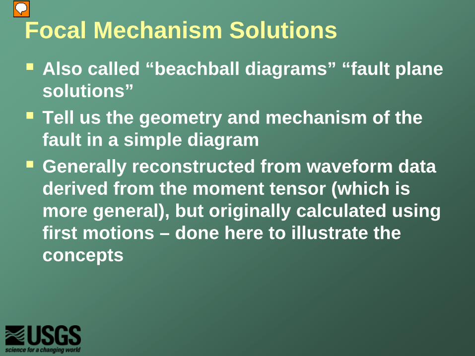
Focal Mechanism SolutionsAlso called “beachball diagrams” “fault plane solutions”Tell us the geometry and mechanism of the fault in a simple diagramGenerally reconstructed from waveform data derived from the moment tensor (which is more general), but originally calculated using first motions – done here to illustrate the concepts
Presenter
Presentation Notes
This session focuses on Focal Mechanism Solutions, often called Beachball diagrams. These are a very commonly used way of graphically representing the fault geometry and slip direction of an earthquake. The original method of constructing beachball diagrams was through the P-wave first motion, this is going to be the method we focus on here as it is the most intuitive to understand. However, now the focal mechanism solutions that are published in catalogs like the NEIC and Harvard CMT are retrieved from calculation of the moment tensor. The moment tensor is a more complete (but non-graphical) method of representing the source mechanism, which the beachball diagram can be extracted from.
Examples
USGS
Presenter
Presentation Notes
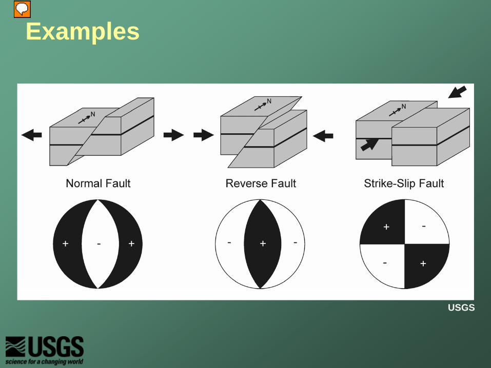
These are examples of the simple cases of strike-slip and pure dip-slip (normal and thrust) motion on a fault. The upper images show block diagrams illustrating the fault motion and the lower images the corresponding fault plane solution. These are the types of diagrams that will be explained during this session.
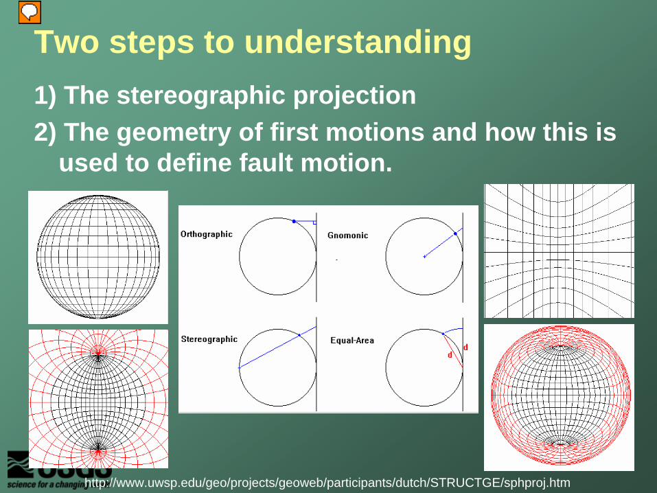
1) The stereographic projection2) The geometry of first motions and how this is
used to define fault motion.
Two steps to understanding
http://www.uwsp.edu/geo/projects/geoweb/participants/dutch/STRUCTGE/sphproj.htm
Presenter
Presentation Notes
There are two stages to understanding these diagrams. The first is the challenge, it’s all about being able to show a 3D problem in 2D. If you can understand the stereographic projection than the focal mechanism solution is only a small additional step. There are several ways of projecting spherical data into a 2D plot, the one we are going to be using is the stereographic projection. In the examples shown on the slide the lower hemisphere is shown in black and the upper (if it can be plotted) is shown in red. The power of the stereographic projection is that angles and shapes are preserved, i.e. the dip of planes or the plunge of linear features are accurately reproduced (this is called “conformal” behavior, the price of this is that the area of objects is distorted.)

Stereographic projectionA method of projecting half a sphere onto a circle.e.g. planes cutting vertically through the sphere plot as straight lines
Images from http://www.learninggeoscience.net/free/00071/index.html
Presenter
Presentation Notes
To visualize the stereographic projection imagine looking straight down onto half a sphere, although this is not exactly the projection it is close enough to help understand what the data plotted using this projection are showing. The easiest data to plot on a stereographic projection are vertical planes. Imagine looking straight down onto a bowl cut by vertical planes, the line where the plane meets the bowl would appear to be a straight line cutting across the bowl. This will be demonstrated with a model in the session. Likewise a plane dipping at any other angle will appear to be a curved line running across the circle, with the amount of curvature varying with the dip of the plane (again this will be demonstrated with a model in the session).
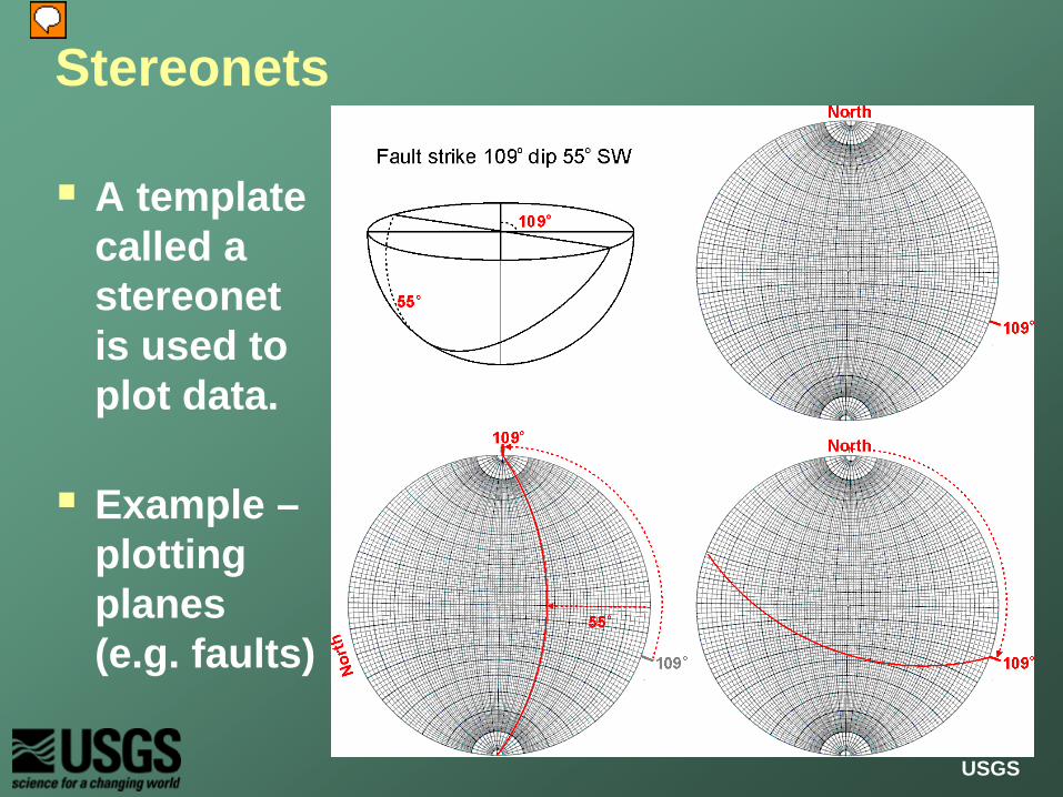
Stereonets
A template called a stereonet is used to plot data.
Example –plotting planes (e.g. faults)
USGS
Presenter
Presentation Notes
The “stereonet” is a template for drawing structures in the stereographic projection. Planes dipping at any angle plot as a line called a “great circle”. The stereonet includes great circles for all angles of dip, but only one azimuth (if all azimuths were drawn the plot would have so many lines it would be impossible to use). But by rotating the stereonet any azimuth can be represented. This slide shows how the stereonet can be used to plot planes of any orientation and dip.
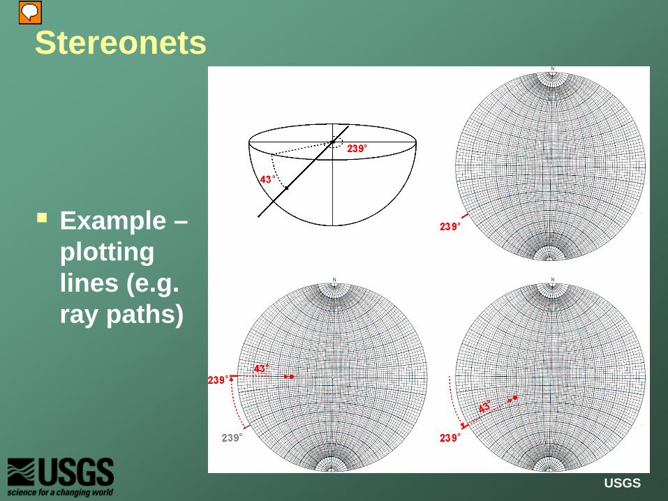
Stereonets
Example –plotting lines (e.g. ray paths)
USGS
Presenter
Presentation Notes
As well as planes the stereonet can also be used to plot lines with a certain plunge and plunge direction. The steps to plot a line are shown in the figure, for the example of a feature with azimuth 239 degrees and plunge of 43 degrees. This is demonstrated during the session with a physical model.
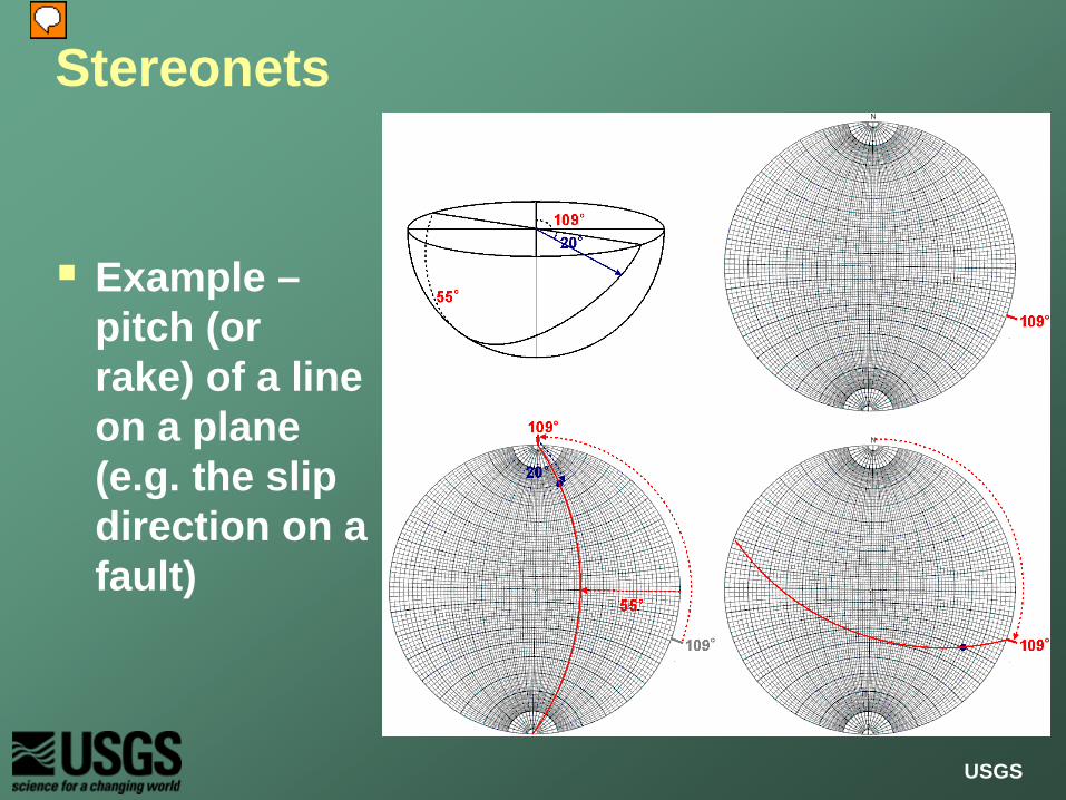
Stereonets
Example –pitch (or rake) of a line on a plane (e.g. the slip direction on a fault)
USGS
Presenter
Presentation Notes
As well as plotting planes and line like features, it is also sometimes useful to describe a line on a plane, for example the slip direction during an earthquake is often given as the slip on the fault plane. The steps for plotting such data are to: 1) Plot the plane, 2) count along the plane the appropriate amount of degrees. This is shown for a feature pitching at -20 degrees on a plane striking at 109 degrees, dipping 55 degrees SW.

Refresher on terminology
USGS
Slip angle is measured from horizontal (positive for thrusts)
Presenter
Presentation Notes
Now we move on to using the stereonet to construct the beachball diagrams that represent the source mechanism. First review terms – hanging wall, footwall, strike, dip, slip, focus, epicenter

Energy and Polarity of “First Motions”
Cox and Hart. Plate Tectonics – How it works.
Presenter
Presentation Notes
The polarity of the first motion at the seismic station provides information on the process that caused the earthquake. In these examples an earthquake caused by an explosion results in ground motion away from the source (compression) in all locations, and an earthquake caused by an implosion results in ground motion towards the source (dilation) in all locations.

Earthquake on a vertical plane
Edited from Cox and Hart. Plate Tectonics – How it works.
Presenter
Presentation Notes
Most earthquakes are double couple, in this situation the first motions are more complex. If we consider a strike slip earthquake on a vertical fault, then the ground motion can be divided into 4 quadrants - 2 with compression and 2 with dilation. The divisions between the compression and dilation are called the “nodal planes”.
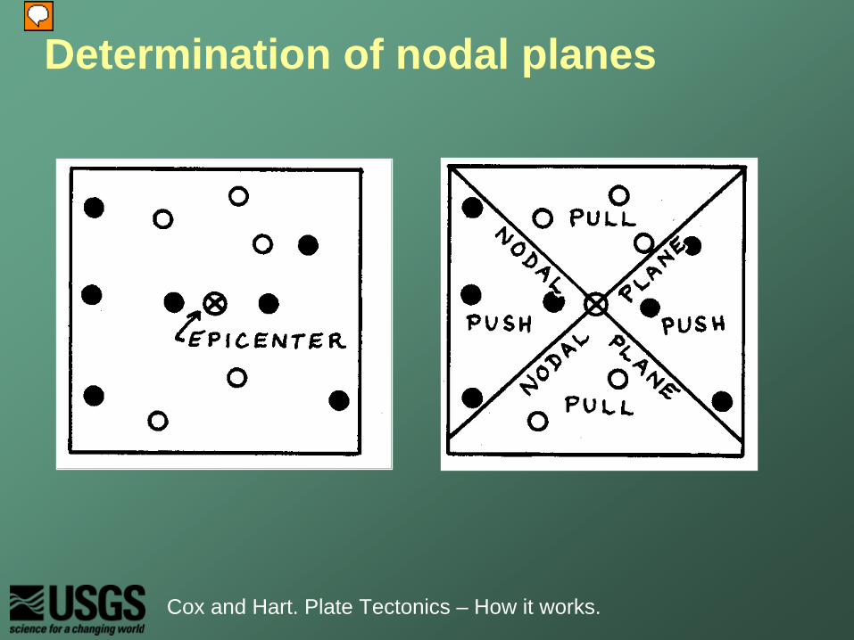
Determination of nodal planes
Cox and Hart. Plate Tectonics – How it works.
Presenter
Presentation Notes
If we had a network of seismic stations around such a strike slip earthquake then the some stations would have a compressional horizontal first motion on the and some would have a dilational motion. The distribution of the first motion can then be used to define the two nodal planes. One of these planes is the fault and the other is known as the “auxiliary plane”, unfortunately the first motions cannot tell us which is which, so we normally turn to the tectonic setting or knowledge of the fault from surface rupture or distribution of other earthquakes, to decide which plane is the fault plane.

Spreading of the seismic wave
Cox and Hart. Plate Tectonics – How it works.

Data on the surface, interpreted in 3D
Cox and Hart. Plate Tectonics – How it works.
Presenter
Presentation Notes
The previous example was for a vertical fault. Now we consider a dipping fault, with a dip slip earthquake. In this case we will also see a pattern of dilation and compression first motions on the surface, which can be interpreted to find the nodal planes, but we have to think in 3-dimensions. For the focal mechanism diagram we construct an imaginary sphere around the fault and each point on the surface of the sphere represents a unique direction from the focus. The ground motion in that direction is then recorded as either compression or dilation. To plot the focal mechanism diagram (beachball) we project half of the sphere onto paper using the stereographic projection.

Take-off angleThe angle (from vertical) that the ray leaves the earthquake = take-off angle
Stein and Wysession, An Introduction to seismology, earthquakes and Earth structure
Presenter
Presentation Notes
To reconstruct the motion at the fault from the first motion recorded at the seismic station we need to know path from the source to the receiver. For most earthquakes most of the stations are relatively distant to the source and so the energy will have traveled down from the focus curving back up to be recorded at the station. Therefore we normally show the lower hemisphere for the focal mechanism diagram. For very locally recorded earthquakes you’ll sometimes see the upper hemisphere plotted so it’s worth checking. In order to construct the diagram we need to know where on the imaginary sphere around the focus the ray path sampled, the angle the ray leaves the source is called the take-off angle and assuming a 1D earth model like PREM the take off angle can be calculated give a know distance between source and receiver.
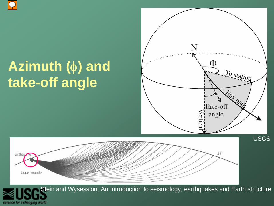
Azimuth (φ) and take-off angle
USGS
Stein and Wysession, An Introduction to seismology, earthquakes and Earth structure
Presenter
Presentation Notes
With azimuth from source to receiver and take-off angle we have a unique point on the sphere around the focus.
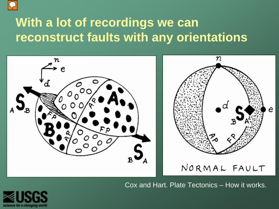
With a lot of recordings we can reconstruct faults with any orientations
Cox and Hart. Plate Tectonics – How it works.
Presenter
Presentation Notes
With enough stations the sphere around the focus will define regions of dilation and compression that define the two nodal planes. This sphere is then represented as the focal mechanism diagram using the stereographic projection.

Fault types and “Beach Ball” plots
USGS
Presenter
Presentation Notes
So returning to our early examples we can see the characteristic patterns of strike slip, normal and thrust faults.

Example Focal mechanism diagrams on mid- ocean ridges
Stein and Wysession, An Introduction to seismology, earthquakes and Earth structure
Presenter
Presentation Notes
With real earthquakes the slip might be oblique, combining strike-slip with dip-slip, then we see a bechball that is a combination of the two.

Same N-S fault, different slip direction
Stein and Wysession, An Introduction to seismology, earthquakes and Earth structure
Presenter
Presentation Notes
These diagrams show how the focal mechanism solution changes with different slip direction on the same north-south fault.

Great review on the web at:
http://www.learninggeoscience.net/free/00071/

By constructing synthetic seismograms and comparing them to the recorded data we use more of the information in the seismogram, not just the arrival time and first motion data
Waveform modeling
Stein and Wysession, “An Introduction to seismology, earthquakes and Earth structure”
Presenter
Presentation Notes
What we’ve talked about so far is using P wave first motions to define the focal mechanism. This is what used to be done in the pre-computer days and is a very good way of learning about focal mechanism solutions as it is relatively easy to understand. P wave first motions are only a small piece of data that can be extracted from the seismogram. The whole waveform can tell us more about the fault process if we can extract the information. So, now we generally use waveform modelling and moment tensor inversion to investigate the source of the earthquake.

Waveform modeling
u(t) = x(t) * e(t) * q(t) * i(t)
seismogram
source time function instrument
responsereflections & conversions at interfaces
attenuation
U(ω)= X(ω) E(ω) Q(ω) I(ω)
Construction of the synthetic seismogram
Stein and Wysession, “An Introduction to seismology, earthquakes and Earth structure”
Presenter
Presentation Notes
The basic idea is that the recorded seismogram is the source function (the signal from the earthquake) modified by its path through the Earth and the imperfect response from the instrument. The effect of the path through the Earth is here divided into two components: e(t) is the effect of reflections and conversions at interfaces and q(t) is the attenuation affect. Each of these factors works as a convolution (*) in the time domain (or multiplication in the frequency domain). The mathematical basis for this theory is called “linear filter theory” and you will often hear the phase “the Earth acts like a filter” used when referring to the affects of attenuation on the waveform.
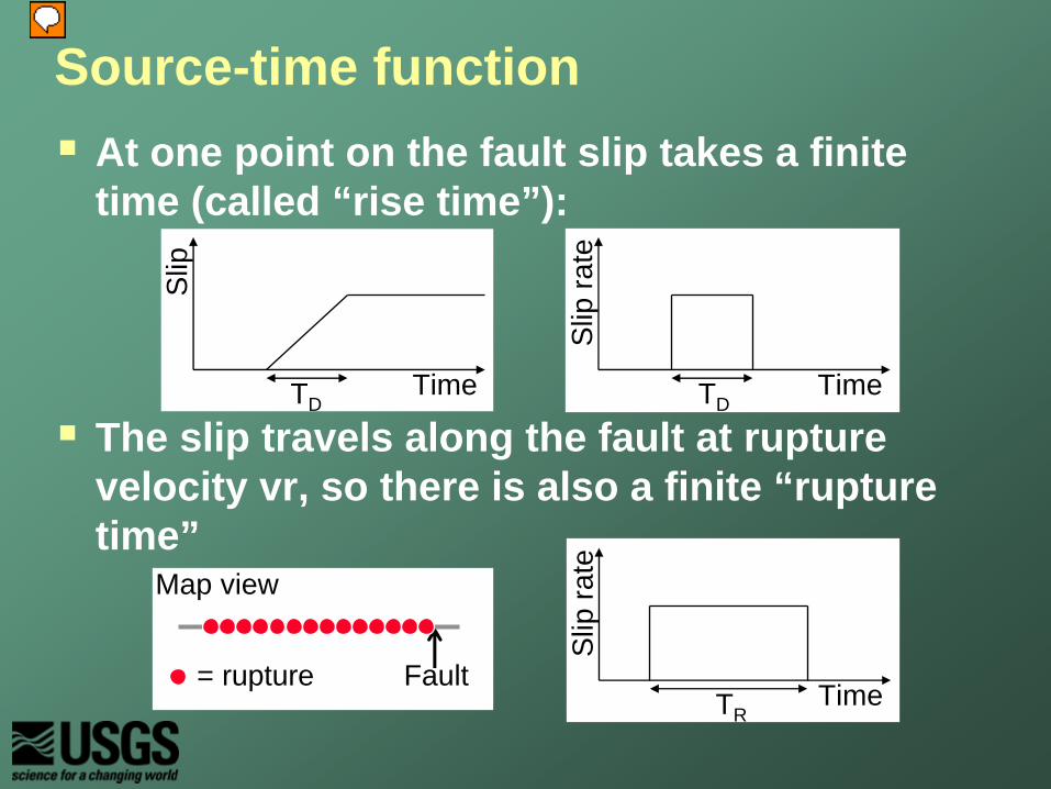
At one point on the fault slip takes a finite time (called “rise time”):
The slip travels along the fault at rupture velocity vr, so there is also a finite “rupture time”
Source-time function
Time
Slip
TDTime
Slip
rate
TD
Time
Slip
rate
TR
Fault= rupture
Map view
Presenter
Presentation Notes
In a simple model of the processes at a fault, the rupture propagates along the fault plane a velocity vr, but in addition to this, at each point of the fault the slip takes a finite amount of time to occur. The finite slip at each point can be modeled as a ramp function (the derivative of this is a boxcar). The propagation of the slip along the fault is also most simply modeled as a boxcar (the duration of which is related to the length of the fault, vr and the direction between the fault and the recording station.

Source time functionThe source time function is the combination of the rise time and the rupture time:
Directionality affects the rupture time
Time
Slip
rate
TDTime
Slip
rate
TR
Slip
rate
TR TD* =
TR TD
TR TD
TR TD
TR TDRupture direction
Presenter
Presentation Notes
The overall source time function is the convolution of the rise time for each component of slip and the rupture time taken for the slip to propagate along the fault. The convolution of 2 boxcars is a trapezoid. The rupture time varies depending on the where the recording station is relative to the fault (“directionality”). If the rupture is propagating towards the station then each new rupture point is closer to the station and so the source time function is bunched-up and appears to be shorter and high amplitude. If the rupture is propagating away from the station the rupture duration is stretched and the source time function is longer and lower amplitude. (The area under the source time function = the seismic moment (Mo), therefore the area is constant for all directions, only the shape changes). This directionality is passed onto the amplitude and duration of the seismogram.

phase reflectionse(t) represents reflections due to the Earth structureIf modeling only the P arrival, it’s only needed for shallow events
Stein and Wysession, “An Introduction to seismology, earthquakes and Earth structure”
Presenter
Presentation Notes
e(t) is a series of pulses representing the conversions and reflections caused by the earth’s structure. Whether this component is important or not depends on exactly what is being modeled and the depth of the earthquake. If we’re only modeling the P arrival and the event is deep then the P will arrive by itself, isolated from other phases and this term is not relevant. However, if the event is shallow then pP and sP will arrive very shortly after P and the waveform will be a combination of all three phases. The diagram shows how the relative polarity of the P and pP varies with the focal mechanism – because the two ray paths leave the focal sphere at different locations the polarity may be different or the same for the two phases, a useful diagnostic.

AttenuationThe loss of energy with time
Q controls the amount of loss
A(t) = A0
e -ω0t/2Q
Sipkin and Jordan 1979, copywrite Seismological Society of America
Presenter
Presentation Notes
Attenuation is the general term for the loss of energy with time. It’s caused by internal frictional during particle motion, which affects high frequencies more rapidly than low frequencies, as they oscillate more times on the same path. The quality factor “Q” controls the amount of energy lost during each cycle. High Q = less energy loss. Q is dependent on the material the wave passes through and the frequency of the wave.

Instrument response function
The response of the seismometer is different for different frequencies so it also filters the data.
Stein and Wysession, “An Introduction to seismology, earthquakes and Earth structure”
Presenter
Presentation Notes
On the figure on the right we see the transfer function of a selection of seismometers, this represents the ability of the instrument to record different frequencies. The line labeled DWWSSN is the response of the old long-period WWSSN instrument, you can see that this instrument only recorded low frequencies over a relatively narrow band. Modern broadband seismometers (e.g. STS-1, STS-2, Guralp-3T) have a flat response (i.e. do not distort the relative amplitude) over a range wide of frequencies; however there are still high and low frequency cut offs. So the instrument cannot perfectly record the seismic arrivals. So when calculating the synthetic waveform we estimate each of these effects, the source-time function, the earth structure and attenuation and the instrument response. Then by combining them in either the time or frequency domain we can create seismogram representing normally the P wave or surface waves. This sort of modeling provides constraints on the source. But we also generate a representation of the source through moment tensor inversion...
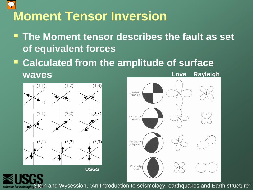
Moment Tensor InversionThe Moment tensor describes the fault as set of equivalent forcesCalculated from the amplitude of surface waves Love Rayleigh
Stein and Wysession, “An Introduction to seismology, earthquakes and Earth structure”
USGS
Presenter
Presentation Notes
By calculating the moment tensor for an earthquake we simplify the source to a set of forces. This means that we don’t have to make assumptions about the fault geometry or slip, we don’t even have to assume the earthquake happened on a fault (the moment tensor can represent any source mechanism, including explosion, implosions, etc). Using assumption about the attenuation and instrument response the forces are calculated that match the surface wave amplitude distribution. The math is quite complicated so we won’t go into it here, but we note that the moment tensor is simplification of the earthquake to a series of forces acting on a point source and is constrained from the surface wave amplitude pattern.