Modeling Uncertainty in Large Natural Resource Allocation...
64
Policy Research Working Paper 9159 Modeling Uncertainty in Large Natural Resource Allocation Problems Yongyang Cai Jevgenijs Steinbuks Kenneth L. Judd Jonas Jaegermeyr omas W. Hertel Development Economics Development Research Group February 2020 Public Disclosure Authorized Public Disclosure Authorized Public Disclosure Authorized Public Disclosure Authorized
Transcript of Modeling Uncertainty in Large Natural Resource Allocation...
Policy Research Working Paper 9159
Modeling Uncertainty in Large Natural Resource Allocation Problems
Yongyang CaiJevgenijs SteinbuksKenneth L. JuddJonas JaegermeyrThomas W. Hertel
Development Economics Development Research GroupFebruary 2020
Pub
lic D
iscl
osur
e A
utho
rized
Pub
lic D
iscl
osur
e A
utho
rized
Pub
lic D
iscl
osur
e A
utho
rized
Pub
lic D
iscl
osur
e A
utho
rized
Produced by the Research Support Team
Abstract
The Policy Research Working Paper Series disseminates the findings of work in progress to encourage the exchange of ideas about development issues. An objective of the series is to get the findings out quickly, even if the presentations are less than fully polished. The papers carry the names of the authors and should be cited accordingly. The findings, interpretations, and conclusions expressed in this paper are entirely those of the authors. They do not necessarily represent the views of the International Bank for Reconstruction and Development/World Bank and its affiliated organizations, or those of the Executive Directors of the World Bank or the governments they represent.
Policy Research Working Paper 9159
The productivity of the world’s natural resources is critically dependent on a variety of highly uncertain factors, which obscure individual investors and governments that seek to make long-term, sometimes irreversible investments in their exploration and utilization. These dynamic considerations are poorly represented in disaggregated resource models, as incorporating uncertainty into large-dimensional prob-lems presents a challenging computational task. This study introduces a novel numerical method to solve large-scale dynamic stochastic natural resource allocation problems
that cannot be addressed by conventional methods. The method is illustrated with an application focusing on the allocation of global land resource use under stochastic crop yields due to adverse climate impacts and limits on further technological progress. For the same model parameters, the range of land conversion is considerably smaller for the dynamic stochastic model as compared to deterministic sce-nario analysis. The scenario analysis can thus significantly overstate the magnitude of expected land conversion under uncertain crop yields.
This paper is a product of the Development Research Group, Development Economics. It is part of a larger effort by the World Bank to provide open access to its research and make a contribution to development policy discussions around the world. Policy Research Working Papers are also posted on the Web at http://www.worldbank.org/prwp. The authors may be contacted at [email protected].

Modeling Uncertainty in Large Natural Resource
Allocation Problems⇤
Yongyang Cai Jevgenijs Steinbuks Kenneth L. Judd
Jonas Jaegermeyr Thomas W. Hertel
JEL: C61, Q15, Q23, Q26, Q40, Q54
Keywords: Dynamic Stochastic Models, Extended Nonlinear Certainty Equivalent Ap-
proximation Method, Crop Yields, Land Use, Natural Resources, Uncertainty
⇤Cai: Department of Agricultural, Environmental and Development Economics, The Ohio State University, [email protected]. Steinbuks: Development Research Group, The World Bank, [email protected]. Judd: Hoover Institution, Stanford University, [email protected]. Jaegermeyr: Department of Computer Science, University of Chicago, NASA Goddard Institute for Space Stud-ies, and Climate Impacts and Vulnerabilities, Potsdam Institute for Climate Impact Research, [email protected]. Hertel: Center for Global Trade Analysis, Purdue University, [email protected]. Cai, Judd, and Hertel appreciate the financial support from United States Department of Agriculture NIFA-AFRI grant 2015-67023-22905; Cai, Steinbuks, and Hertel appreciate the financial support from the National Science Foundation (SES-0951576 and SES-1463644) under the auspices of the RDCEP project at the Uni-versity of Chicago. Cai would also like to thank Becker Friedman Institute at the University of Chicago and Hoover Institution at Stanford University for their support. This research is part of the Blue Waters sustained-petascale computing project, which is supported by the National Science Foundation (awards OCI-0725070 and ACI-1238993) and the State of Illinois. Blue Waters is a joint e↵ort of the University of Illinois at Urbana-Champaign and its National Center for Supercomputing Applications. Earlier versions of this paper include “The E↵ect of Climate and Technological Uncertainty in Crop Yields on the Optimal Path of Global Land Use” and “Optimal Path for Global Land Use under Climate Change Uncertainty”.
1 Introduction
Understanding the allocation of the world’s natural resources over the course of the next
century is an important research problem for agricultural and environmental economists.
Analyzing natural resources use in the long run involves a complex interplay of di↵erent
factors. These factors include, among others, continuing population increases, shifting di-
ets among the poorest populations in the world, increasing the production of renewable
energy, including biofuels, and growing demand for ecosystem services, including forest car-
bon sequestration (Foley et al., 2011). The problem is further confounded by faster than
expected climate change, which is altering the biophysical environment of agriculture and
forestry. Moreover, highly uncertain future productivities and valuations of ecosystem ser-
vices, coupled with medium- to long-term irreversibilities in the extraction of nonrenewable
or partially renewable resources, such as natural forests,1 give rise to a challenging problem
of decision-making under uncertainty.
While there is a large body of economic literature analyzing the problem of natural
resource extraction and utilization under uncertainty theoretically or using stylized compu-
tational models (see e.g., Miranda and Fackler (2004), Tsur and Zemel (2014) and references
therein), quantifying the e↵ects of uncertainty on natural resource use in a more realistic
setting remains a challenging problem. This is because natural resource allocation prob-
lems, like environmental policy problems in general, involve highly nonlinear structure and
damage functions, important irreversibilities, and long time horizons (Pindyck, 2007). Com-
putational integrated models of the economy and environment are the standard workhorse
mechanisms for modeling the long term allocation of the world’s natural resources, including
particularly di�cult land use problems.2 These models have the important advantage of
detailed spatial and sectoral (particularly, energy and agricultural sector) coverage, which
allows them to capture a broad range of responses to changes in demand and supply factors
a↵ecting utilization of natural resources. However, given the high computational complexity
of these models, they are typically either static or based on myopic expectations, whereby
decisions about production, consumption and resource extraction and conversion are made
only on the basis of information in the period of the decision (Babiker et al., 2009). These
models, therefore, have limited ability to address important intertemporal questions such as,
for example, a dynamic trade-o↵ between conservation, carbon sequestration, and renewable
o↵sets for fossil fuels. Among the few forward-looking, dynamic economy and environment
models, none explicitly incorporates uncertainty into the determination of the optimal path
of natural resource use.3 This is because introducing uncertainty into these models is con-
fined by an array of computational obstacles that are very di�cult (e.g., high dimensionality
and kinks caused by occasionally binding constraints), if not impossible, to address using
1The biophysical and ecological literature suggests that restoration of forest structure and plant speciestakes at least 30–40 years and usually many more decades (Chazdon, 2008), costs several to $10,000 perhectare (Nesshover et al., 2009), and is only partially successful in achieving reference conditions (Benayaset al., 2009).
2For a detailed overview of these models and their applications to natural resources and land use problems,see, e.g., Fussel (2009), Schmitz et al. (2014), and Nikas et al. (2019).
3Several recent studies, most notably, Cai and Lontzek (2019) have successfully integrated uncertaintyabout economic and climate outcomes in a stochastic integrated assessment climate-economy framework.For a review of this related literature, see Cai (2019).
2
standard computational methods in economics such as projection methods and value func-
tion iteration (see, e.g., Judd 1998; Miranda and Fackler 2004; Cai and Judd 2014; Cai
2019). To the extent that uncertainty in these models is considered, this is only through
parametric or probabilistic sensitivity analysis or the use of alternative scenarios. Therefore,
the high-dimensional resource use models have not e↵ectively dealt with optimal extraction
and conversion decisions along the uncertain path of key drivers a↵ecting resource allocation
in the face of costly reversal of conversion decisions.
In this study, we seek to address this important limitation of the economy-environment
modeling of natural resource use. In doing so, we build on Cai et al. (2017), who have
introduced a nonlinear certainty equivalent approximation method (NLCEQ) for solving
large-scale infinite horizon stationary dynamic stochastic problems and demonstrated how
this method could be used to achieve the accurate solution to a stylized stationary dynamic
stochastic land use problem. While the original NLCEQ method can successfully solve
many complicated problems in other fields of economics, particularly, macroeconomics, it
has very limited applicability for solving environmental and resource economics problems.
This is because many stochastic problems of utilization of natural resources feature nonsta-
tionary stochastic trends, such as, e.g., climate or technological trajectories, and some never
converge to a stationary state. This paper introduces a novel algorithm, called Extended NL-
CEQ (ENLCEQ), that advances the original NLCEQ work to solve nonstationary dynamic
stochastic problems and apply it to solve more complex dynamic stochastic multi-sectoral
resource use problems with exogenous trends. Similar to the original NLCEQ method,
the ENLCEQ method approximates the true solution to the underlying dynamic stochastic
problem with globally valid, nonlinear certainty-equivalent decision rules. These rules are
then used to generate simulation paths for nonstationary infinite or finite horizon resource
use problems. In this paper, we show that the ENLCEQ approximation is highly accurate
and achieves stable numerical solutions.
We illustrate the ENLCEQ method to solve for the dynamic optimal global land use
allocation, which is a highly complicated resource use problem that features multiple cross-
sectoral and dynamic trade-o↵s. Specifically, we apply the method to a global land use
model nicknamed FABLE (Forest, Agriculture, and Biofuels in a Land use model with
Environmental services) in the face of uncertainty.4 FABLE is a dynamic, forward-looking
global multi-sectoral partial equilibrium model designed to analyze the evolution of global
land use over the coming century. Prior applications of that model (Steinbuks and Hertel,
2013; Hertel et al., 2013, 2016; Steinbuks and Hertel, 2016) analyze competition for scarce
global land resource in light of growing demand for food, energy, forestry and environmental
services, and evaluate key drivers and policies a↵ecting global land use allocation. All
these applications, however, assume perfect foresight, and treat uncertainty in a parametric
fashion, thus ignoring the impact of future uncertainties on the optimal allocation of global
land use.
By way of illustration, we choose to focus on uncertainty emanating from crop produc-
tivity over the next century. Along with energy prices, regulatory policies, and technological
4To evaluate the method’s accuracy, we also apply it to a simpler optimal growth model shown in theonline appendix.
3
change in food, timber and biofuels industries, this is one of four core uncertainties a↵ecting
competition for global land use (Steinbuks and Hertel, 2013). To quantify the uncertainty
in agricultural yields, we construct stochastic crop productivity index that captures two key
uncertainty sources: technological progress and global climate change (Lobell et al., 2009;
Licker et al., 2010; Foley et al., 2011).5 Following Rosenzweig et al. (2014), we use projec-
tions from climate and crop simulation models, as well as the survey of recent agro-economic
and biophysical studies to calibrate the index.
We simulate the results of the perfect foresight model under di↵erent realizations of the
crop productivity index, focusing our attention on the current century. We then compare
and contrast them with the results of the dynamic stochastic model, where the uncertainty
in crop yields is brought to the model’s optimization stage. When the uncertainty in crop
productivity is incorporated into the model, we see an additional redistribution of land
resources aimed at o↵setting the impact of potentially lower yields. Owing to intertempo-
ral substitution, some of that redistribution takes place even in the absence of the actual
changes in the states of climate or technology a↵ecting crop yields. Moreover, the range of
these alternative optimal paths of cropland is considerably smaller than the magnitude of
possible land conversion resulting from the scenario analysis based on deterministic model
simulations. This result indicates that the scenario analysis may significantly overstate the
magnitude of expected agricultural land conversion under uncertain crop yields.
Besides the methodological innovation, our study also contributes to the growing envi-
ronmental economics literature that analyzes the intertemporal allocation of land and other
natural resources under uncertainty and irreversibility constraints. Most of that literature
focuses on a particular type of resource or sector, where intertemporal issues are significant
and cannot be ignored. One example of this literature is forestry management in the con-
text of uncertain fire risks and climate mitigation policies (Sohngen and Mendelsohn, 2003,
2007; Daigneault et al., 2010). Another example is natural land conservation decisions un-
der irreversible biodiversity losses (Conrad, 1997, 2000; Bulte et al., 2002; Leroux et al.,
2009). While these models are undoubtedly helpful for understanding the broad implica-
tions of uncertainty on the intertemporal allocation of land resources, they fail to account
for the e↵ect of uncertainty in supply and demand drivers on the optimal allocation of land
resources in the long run. Our study is perhaps most closely related to the recent work of
Lanz et al. (2017) who develop a two-sector stochastic Schumpeterian growth model with
the endogenous allocation of global land use. They find, like our paper does, that optimal
allocation of global land use requires more cropland conversion when the uncertainty in
agricultural productivity is present. Lanz et al. (2017), however, focused on endogenous
population dynamics, labor allocation, and technological progress, whereas our paper is
concerned about the endogenous allocation of multiple types of land use and correspond-
ing land-based goods and services. Our paper also advances on methodological grounds
by introducing a novel algorithm that overcomes the computational di�culties of solving
multidimensional stochastic land use models, which made Lanz et al. (2017) significantly
5Climate change will likely a↵ect the productivity of other land resources, such as forestland. Severalrecent modeling studies (see, e.g., Tian et al. (2016) and references therein) have suggested that climatechange is likely to result in higher forest growth and greater timber yields, as well as in more forest dieback,with the net e↵ects varying over time and space. Incorporating these e↵ects is beyond the scope of thisstudy and is left for future research.
4

simplify their model by assuming that their binary shocks occur only in three time periods.
2 Extended NLCEQ
Following the standard notation in the literature, let St be a vector of state variables (e.g.,
natural resource stock), and at be a vector of decision variables (e.g., resource extraction,
transformation, and final consumption) at each time t. The transition law of the state vector
S is
St+1 = Gt(St,at, ✏t)
where ✏t is a serially uncorrelated random vector process,6 and Gt is a vector of functions:
its i-th element, Gt,i, returns the i-th state variable at t + 1: St+1,i. For simplicity, we
assume the mean of ✏t is 0.7
We solve the following social planner’s problem:
maxat2Dt(St)
E(
T⇤�1X
t=0
�tUt (St,at) + �T⇤VT⇤(ST⇤)
)(1)
s.t. St+1 = Gt(St,at, ✏t), t = 0, 1, 2, ..., T ⇤ � 1,
S0 given
where Ut is a utility function, � 2 (0, 1) is the discount factor, E is the expectation operator,
T ⇤ is the horizon (T ⇤ = 1 if it is an infinite-horizon problem), VT⇤(ST⇤) is a given terminal
value function depending on the terminal state ST⇤ (it is zero everywhere for an infinite-
horizon problem), and Dt(St) is a feasible set of actions at at time t. And we assume that
the initial state S0 is given, as it can usually be observed or estimated.
In most economic problems of resource use under uncertainty, the social planner’s prob-
lem cannot be solved analytically, although certain inferences about potential e↵ects of
uncertainty can be made from more stylized models.8 Numerical dynamic programming
with value function iteration (see, e.g., Cai and Judd 2014; Cai 2019) is a typical method to
solve these dynamic stochastic problems. However, numerical dynamic programming faces
challenging problems such as high dimensionality of state space, shape-preservation of value
functions (Cai and Judd, 2013), and occasionally binding constraints. These challenges
are common in modeling natural resource use and are hard to address even with the most
advanced methods, such as parallel dynamic programming (Cai et al., 2015). Below we in-
troduce a new algorithm, called the extended nonlinear certainty equivalent approximation
6In dynamic models with serially correlated random variables, they should be exogenous state variables,and we can use an uncorrelated vector ✏t in their transition laws.
7For notational simplicity we keep the same mathematical representation of a transition function evenif some of its elements are redundant. For example, if Gt,i is deterministic, we still denote it as St+1,i =
Gt,i(St,at, ✏t) even though St+1,i = eGt,i(St,at) + 0 · ✏t. Similarly, if there are some unused elements of ✏tor some redundant arguments in a function Gt,j , we can multiply them by zero in Gt,j and thus still useSt+1,j = Gt,j(St,at, ✏t) .
8Pindyck (1984) shows that stochastic fluctuations add a risk premium to the rate of return required tokeep a unit of renewable resource stock in situ. Conrad (2000) demonstrates that the presence of uncertaintyover benefits and opportunity costs of extracting natural forest land attaches option value for wildernesspreservation, and may require a higher return on development to induce deforestation. Daigneault et al.(2010) argue that the presence of uncertainty over forest fire requires more frequent thinning and shorterrotations of managed forests.
5
method (ENLCEQ), that extends the original NLCEQ method of Cai et al. (2017) designed
primarily for solving dynamic stochastic stationary problems in macroeconomics. Later in
this study, we apply this method to solve a complicated dynamic stochastic land use prob-
lem, that features high dimensionality, occasionally binding constraints, and time-varying
exogenous trends, with acceptable accuracy. It is important to note that although the focus
of this study is on stochastic natural resource allocation problems, the ENLCEQ method
is a general method that can be applied to approximately and numerically solve dynamic
stochastic problems in other areas of the economics discipline.
The original NLCEQ method computes globally valid, nonlinear certainty-equivalent
decision rules, and then uses them to generate simulation paths for stationary infinite horizon
problems. For non-stationary problems, this involves computing such rules at each period t
along time-variant exogenous paths a↵ecting decisions. However, computing all these rules
can be very time-consuming and unnecessary if our primary goal is to obtain simulation
paths and their distributions until a time of interest, T , even a long one (in environmental
and climate change economics, for example, we are often interested in solutions for the
coming century, and set the time of interest to 100 years and the problem horizon of more
than 300 years to avoid a large impact of terminal conditions). Instead of solving for optimal
decisions for all possible states at each time, we can approximately solve for optimal decisions
for those simulated states along simulated paths. Thus, we introduce the following ENLCEQ
algorithm.
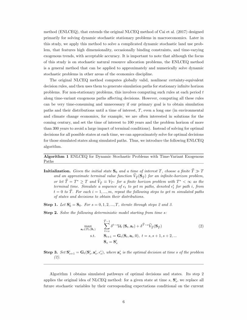
Algorithm 1 ENLCEQ for Dynamic Stochastic Problems with Time-Variant ExogenousPaths
Initialization. Given the initial state S0 and a time of interest T , choose a finite bT � Tand an approximate terminal value function eVbT (SbT ) for an infinite-horizon problem,
or let bT = T ⇤ � T and eVbT ⌘ VT⇤ for a finite horizon problem with T ⇤ < 1 as theterminal time. Simulate a sequence of ✏t to get m paths, denoted ✏it for path i, fromt = 0 to bT . For each i = 1, ...,m, repeat the following steps to get m simulated pathsof states and decisions to obtain their distributions.
Step 1. Let Si0 = S0. For s = 0, 1, 2, ..., T , iterate through steps 2 and 3.
Step 2. Solve the following deterministic model starting from time s:
maxat2Dt(St)
bT�1X
t=s
�t�sUt (St,at) + �bT�s eVbT (SbT ) (2)
s.t. St+1 = Gt(St,at, 0), t = s, s+ 1, s+ 2, ...
Ss = Sis
Step 3. Set Sis+1 = Gt(Si
s,ais, ✏
is), where ais is the optimal decision at time s of the problem
(2).
Algorithm 1 obtains simulated pathways of optimal decisions and states. Its step 2
applies the original idea of NLCEQ method: for a given state at time s, Sis, we replace all
future stochastic variables by their corresponding expectations conditional on the current
6

state Sis,
9 and convert the dynamic stochastic problem (1) into a deterministic finite-horizon
dynamic problem (2).
For an infinite-horizon problem, step 2 changes it to be a finite-horizon problem with a
large horizon bT . This will have little impact on the solutions within the period of interest:
[0, T ], because (i) most of infinite-horizon dynamic economic models assume that the system
asymptotically evolves to its stationary state; (ii) the discount factor � < 1 makes the
terms �t�TUt (St,at) to have small magnitude for t � bT with a large bT and a feasible
and reasonable sequence of (St,at) so that the terms after bT has little changes on the
objective function; (iii) we choose bT to be large enough such that any larger bT will almost
have no change in the solutions in the periods of interest [0, T ]; and (iv) we may choose a
good approximate terminal value function such as eVbT (SbT ) = UbT
⇣SbT , ea
⇤bT(SbT )
⌘/(1 � �) to
approximate the true value function at bT : VbT (SbT ) = maxP1
t=bT �t�bTUt (St,at) subject to
the transition law of St and the feasibility constraint for at, where ea⇤bT (SbT ) is a good guess
of the true optimal policy function at bT .In step 2 of Algorithm 1, we drop the uncertainty in the transition law of St of the original
problem (1) by replacing ✏t by its zero mean, so that the expectation in the objective function
of (1) is cancelled. We call this a certainty equivalent approximation.10
We implement the optimal control method to solve (2) numerically, that is, we view
(2) as a large-scale nonlinear constrained optimization problem with {ait : t � s} and
{Sit : t � s} as its decision and state variables. The problem can be directly solved with
an appropriate nonlinear optimization solver such as CONOPT (Drud, 1994).11 Observe
that we just need to keep the solution at time s, ais, for use in the next step. In step 3
of Algorithm 1 we use the optimal decision ais to generate the next-period state, Sis+1 =
Gt(Sis,a
is, ✏
is), given realization of shocks, ✏is. Once we reach the state Si
s+1 at time s + 1,
we come back to implement step 2 and then step 3. In other words, Algorithm 1 uses
an adaptive management way: decisions are made for the current period in the face of
the future uncertain shocks; once the next-period shock is observed, decisions for the next
period are made with re-optimization given the observed shock and new state variables at
the next period. Observe that the serial correlation of random variables has been captured
in their associated transition laws. Repeating this process iteratively through T times,
9As ✏t is a serially uncorrelated stochastic process, we can replace ✏t by its zero mean in the functionsof Ft and Gt in (2) if all transition laws are continuous. For problems with a discrete Markov chain intransition laws, we can use the same technique as described in Cai et al. (2017) for NLCEQ with a discretestochastic state to obtain the corresponding deterministic model (1). That is, given realization of the Markovchain at time s, we can compute expectations of the Markov chain at all times after s conditional on thevalue at time s and then replace the stochastic process by the path of the conditional expectations in step2 of Algorithm 1.
10If the utility Ut is a common power function with a relative risk aversion parameter �, then the role ofthe risk aversion disappears in the certainty equivalent approximation model (2). As � is also the inverseof the intertemporal elasticity of substitution (IES) for time-separable power utilities, the IES, 1/�, stilla↵ects the solution to the deterministic model (2). For this reason, the NLCEQ and the ENLCEQ methodscannot work for dynamic portfolio problems, where the risk aversion is important for risky portfolio choices,dynamic stochastic problems with Epstein–Zin preferences (e.g., Cai and Lontzek (2019)) in which the riskaversion and the IES are separated, or static problems, where � has only the risk aversion role. For thestochastic land use problem in the next section and the optimal growth model in the appendix, we usetime-separable utilities, so the ENLCEQ is an appropriate method. As we cannot a priori determine theimplications of certainty equivalence assumption on the solution accuracy, we should always check the errorsof solutions of ENLCEQ. As we show below, for examples analyzed in this study, the solution errors areminimal.
11See Cai (2019) for discussion on the optimal control method.
7
we compute a representative simulated pathway of optimal decisions, {ais}Ts=0, and states,
{Sis}Ts=0, which corresponds to the realized path of shocks, {✏is}Ts=0. Repeating over i, we
compute m simulated paths of optimal states and decisions, (St,at), from time 0 to T , and
then obtain their distributions. This simulation process can be naturally parallelized.12
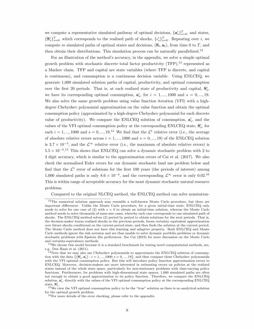
For an illustration of the method’s accuracy, in the appendix, we solve a simple optimal
growth problem with stochastic discrete total factor productivity (TFP),13 represented as
a Markov chain. TFP and capital are state variables (where TFP is discrete, and capital
is continuous), and consumption is a continuous decision variable. Using ENLCEQ, we
generate 1,000 simulated solution paths of capital, productivity, and optimal consumption
over the first 20 periods. That is, at each realized state of productivity and capital, Sis,
we have its corresponding optimal consumption, ais, for i = 1, ..., 1000 and s = 0, ..., 19.
We also solve the same growth problem using value function iteration (VFI) with a high-
degree Chebyshev polynomial approximation on the value function and obtain the optimal
consumption policy (approximated by a high-degree Chebyshev polynomial for each discrete
value of productivity). We compare the ENLCEQ solution of consumption, ais, and the
values of the VFI optimal consumption policy at the corresponding ENLCEQ state, Sis, for
each i = 1, ..., 1000 and s = 0, ..., 19.14 We find that the L1 relative error (i.e., the average
of absolute relative errors across i = 1, ..., 1000 and s = 0, ..., 19) of the ENLCEQ solution
is 3.7 ⇥ 10�3, and the L1 relative error (i.e., the maximum of absolute relative errors) is
5.5⇥ 10�3.15 This shows that ENLCEQ can solve a dynamic stochastic problem with 2 to
3 digit accuracy, which is similar to the approximation errors of Cai et al. (2017). We also
check the normalized Euler errors for our dynamic stochastic land use problem below and
find that the L1 error of solutions for the first 100 years (the periods of interest) among
1,000 simulated paths is only 8.6 ⇥ 10�4, and the corresponding L1 error is only 0.02.16
This is within range of acceptable accuracy for the most dynamic stochastic natural resource
problems.
Compared to the original NLCEQ method, the ENLCEQ method can solve nonstation-
12The numerical solution approach may resemble a well-known Monte Carlo procedure, but there areimportant di↵erences. Unlike the Monte Carlo procedure, for a given initial-time state, ENLCEQ onlyneeds to solve for one case of (2) with s = 0 to obtain an initial-time solution, whereas the Monte Carlomethod needs to solve thousands of same-size cases, whereby each case corresponds to one simulated path ofshocks. The ENLCEQ method solves (2) period by period to obtain solutions for the next periods. That is,the decision-maker learns realized shocks in the previous periods, forms certainty equivalent approximationover future shocks conditional on the current-period state, and then finds the solution at the current period.The Monte Carlo method does not have this learning and adaptive property. Both ENLCEQ and MonteCarlo methods ignore the risk aversion and are thus unable to solve dynamic portfolio problems or dynamicstochastic problems with Epstein–Zin preferences. See Cai (2019) for more discussion on the Monte Carloand certainty-equivalence methods.
13We choose this model because it is a standard benchmark for testing novel computational methods, see,e.g., Den Haan et al. (2011).
14Note that we may also use Chebyshev polynomials to approximate the ENLCEQ solution of consump-tion with the data
��Sis,a
is
�: i = 1, ..., 1000; s = 0, ..., 19
, and then compare these Chebyshev polynomials
with the VFI optimal consumption policy. But this will introduce policy function approximation errors toENLCEQ. Moreover, decision-makers are more interested in estimating errors on policies at the realizedstates instead of the whole state space, particularly for non-stationary problems with time-varying policyfunctions. Furthermore, for problems with high-dimensional state spaces, 1,000 simulated paths are oftennot enough to obtain a good approximation to its policy function. Therefore, we compare the ENLCEQsolution, ai
s, directly with the values of the VFI optimal consumption policy at the corresponding ENLCEQstate, Si
s.15We view the VFI optimal consumption policy to be the “true” solution as there is no analytical solution
for the optimal growth problem.16For more details of the error checking, please refer to the appendix.
8
ary problems which the NLCEQ method cannot unless it is applied at every period t. Even
for stationary problems, ENLCEQ does not require explicit approximation of the optimal
decision rules so it may be more suitable for implementation of high-dimensional problems
that require sparse grid approximation and are di�cult to code. Moreover, ENLCEQ is
more e�cient than the original NLCEQ method, if the number of simulations, m, is less
than the number of approximation nodes used in the original NLCEQ method. For exam-
ple, for the dynamic stochastic model of global land use in this study, it has 15 continuous
state variables and 2 discrete state variables (totally 5 ⇥ 3 = 15 discrete states). If we use
only 5 nodes per continuous state variable to get degree-4 complete Chebyshev polynomial
approximation, NLCEQ needs to solve 515⇥15 ⇡ 4.6⇥1011 optimization problems at every
period t. Even if we use only 3 nodes per continuous state variable to get a quadratic poly-
nomial approximation, NLCEQ needs to solve 315 ⇥ 15 ⇡ 2.2 ⇥ 108 optimization problems
at every period t. The ENLCEQ method only needs to solve m optimization problems at
every period t. Typically we can choose m = 1, 000, so it is about 22,000 times faster than
NLCEQ with quadratic polynomial approximation, or 4.6⇥ 108 times faster than NLCEQ
with degree-4 polynomial approximation. Furthermore, because the ENLCEQ method does
not use an explicit approximation to continuous value / policy functions, there are no func-
tional approximation errors, and solutions from ENLCEQ may be more accurate than those
from the original functional approximation-based NLCEQ method.
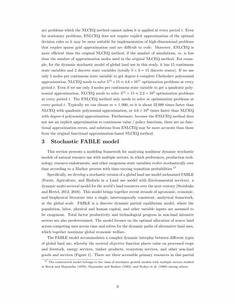
3 Stochastic FABLE model
This section presents a modeling framework for analyzing nonlinear dynamic stochastic
models of natural resource use with multiple sectors, in which preferences, production tech-
nology, resource endowments, and other exogenous state variables evolve stochastically over
time according to a Markov process with time-varying transition probabilities.17
Specifically, we develop a stochastic version of a global land use model nicknamed FABLE
(Forest, Agriculture, and Biofuels in a Land use model with Environmental services), a
dynamic multi-sectoral model for the world’s land resources over the next century (Steinbuks
and Hertel, 2012, 2016). This model brings together recent strands of agronomic, economic,
and biophysical literature into a single, intertemporally consistent, analytical framework,
at the global scale. FABLE is a discrete dynamic partial equilibrium model, where the
population, labor, physical and human capital, and other variable inputs are assumed to
be exogenous. Total factor productivity and technological progress in non-land intensive
sectors are also predetermined. The model focuses on the optimal allocation of scarce land
across competing uses across time and solves for the dynamic paths of alternative land uses,
which together maximize global economic welfare.
The FABLE model accommodates a complex dynamic interplay between di↵erent types
of global land use, whereby the societal objective function places value on processed crops
and livestock, energy services, timber products, ecosystem services, and other non-land
goods and services (Figure 1). There are three accessible primary resources in this partial
17 The constructed model belongs to the class of stochastic growth models with multiple sectors studied
in Brock and Majumdar (1978), Majumdar and Radner (1983), and Stokey et al. (1989) among others.
9

Utility
FossilFuels
UnmanagedForests
CropLand
RawTimber
1stGen.Biofuels
ProtectedForests
ManagedForests
Fertilizers
FoodCropsBiofuels’CropsAnimalFeed
OtherPrimaryInputs
PetroleumProducts
ProcessedCrops
EcosystemServices
EnergyServices
OtherG&S
ProcessedTimber
PrimaryInputs
Intermediateproducts
FinalGoods
PastureLand
ProcessedLivestock
Livestock 2ndGen.Biofuels
TechnologicalProgress,ClimateChange
Figure 1: Structure of the FABLE Model
Note. State variables, St are shown as oval shapes. Decision variables, at, are shown as rectangularshapes. Utility function, Ut, is shown as octagonal shape. Transition laws, Gt, are shown as dottedarrows. Stochastic model terms incorporating random processes, ✏t, are shown as dashed shapes orarrows.
10

equilibrium model of the global economy: land, liquid fossil fuels, and other primary inputs,
e.g., labor and capital (see the bottom part of Figure 1). The supply of land is fixed and
faces competing uses that are determined endogenously by the model. They include un-
managed forest lands - which are in an undisturbed state (e.g., parts of the Amazon tropical
rainforest ecosystem), agricultural (or crop) land, pasture land, and commercially managed
forest land.18 As trees of di↵erent age have di↵erent timber yields and di↵erent propensities
to sequester carbon, the model keeps track of various tree vintages in managed forests,19
which introduces additional numerical complexity for solving the model. The flow of liquid
fossil fuels evolves endogenously along an optimal extraction path, allowing for exogenously
specified new discoveries of fossil fuel reserves. Other primary inputs include variable in-
puts, such as labor, capital (both physical and human), and intermediate materials. The
endowment of other primary inputs is exogenous and evolves along a pre-specified global
economic growth path.
There are six intermediate inputs used in the production of land-based goods and ser-
vices in FABLE: petroleum products, fertilizers, crops, liquid biofuels,20 live animals, and
raw timber (see the middle part of Figure 1). Fossil fuels are refined and converted to either
petroleum products, that are further combusted, or to fertilizers, that are used to boost
yields in the agricultural sector. Cropland and fertilizers are combined to grow crops, that
can be further converted into processed food and biofuels, or used as an animal feed. Specif-
ically, we assume that agricultural land LA,ct and fertilizers xn,c
t are imperfect substitutes
in production of food crops, xct , with specific production technology given by the following
constant elasticity of substitution (CES) function:
xct = ✓ct
⇣↵n
⇣LA,ct
⌘⇢n
+ (1� ↵n) (xn,ct )
⇢n
⌘ 1⇢n
, (3)
where ✓ct is stochastic crop technology index, and ↵n and ⇢n are, respectively, the input share
and substitution parameters. Equation (3) captures three key responses within the model
to changes in crop technology index: (i) demand response (change in consumption of food
crops), (ii) adaptation on the extensive margin (substitution of agricultural land for other
land resources), and (iii) adaptation on the intensive margin (substitution of agricultural
land for fertilizers).
The biofuels substitute imperfectly for liquid fossil fuels in final energy demand. The
food crops used as animal feed and pasture land are combined to produce raw livestock.
Harvesting managed forests yield raw timber, that is further used in timber processing.
The land-based consumption goods and services take the form of processed crops, live-
stock, and timber, and are, respectively, outcomes of food crops, raw livestock and timber
18We ignore other land use types, such as savannah, grasslands, and shrublands, which are largely unman-aged and often of limited productivity. This makes them di�cult to incorporate into an economic model ofland use. Consequently, they are typically left out of most contemporary analyses of global land use change(Hertel et al., 2009). We also ignore residential, retail, and industrial uses of land in this partial equilibriummodel of agriculture and forestry.
19We do not keep track of vintages for natural lands and assume they are primarily old grown forest.20In FABLE, bioenergy does not include the potential use of biomass in power generation. This limitation
is acknowledged in Steinbuks and Hertel (2016, p. 566): “A more serious limitation to this study is ouromission of the potential demand for biomass in power generation. Under some scenarios, authors haveshown this to be an important source of feedstock demand by mid-century (Rose et al. 2012). However,absent a full representation of the electric power sector, our framework is ill-suited to addressing this issue.”
11
processing. The production of energy services combines non-land energy inputs (i.e., liquid
fossil fuels) with the biofuels, and the resulting mix is further combusted. Finally, all land
types have the potential to contribute to other ecosystem services, a public good to society,
which includes recreation, biodiversity, and other environmental goods and services.21 To
close the demand system, we also include other non-land goods and services (e.g., manu-
facturing goods and retail, construction, financial, and information services), which involve
’consumption’ of other primary inputs not spent on the production of land-based goods and
services. As the model focuses on the representative agent’s behavior, the final consumption
products are all expressed in per-capita terms.
To preserve space, a complete description of model equations, variables, and parameter
values is presented in the online appendix.
4 Modeling Crop Yield Uncertainty
This section characterizes uncertainty in future agricultural yields over the coming century,
which is one of the core uncertainties shown to a↵ect land use in the long run (Steinbuks
and Hertel, 2013). Crop yields are subject to two types of uncertainties: those related to
the development and dissemination of new technologies, and those related to changes in the
climatic conditions under which the crops are grown. The former type of uncertainty has
until recently dominated the pattern of the evolution of the global crop yields, whereas the
latter is becoming an increasingly important factor (Lobell and Field, 2007; IPCC, 2014a).
While it is plausible to hypothesize that accelerating climate impacts may, in turn, induce
further technological advances in an e↵ort to facilitate adaptation to climate change, this
hypothesis is not supported by limited empirical evidence.22 Therefore, in this paper, these
two sources of uncertainty are treated separately, although they are both characterized by
the use of combined climate and crop simulation models run over a global grid.
We characterize future uncertainty in yields by constructing a stochastic crop productiv-
ity index, ✓ct , which captures the evolution of future crop yields under di↵erent realizations
of uncertainty in crop productivity based on the most recent projections in the agronomic
and environmental science studies. An important characteristic of staple grains yields is
that they tend to grow linearly, adding a constant amount of gain (e.g., ton/ha) each year
(Grassini et al., 2013). This suggests that the proportional growth rate should fall gradu-
ally over time. However, crop physiology dictates certain biophysical limits to the rate at
which sunlight and soil nutrients can be converted to the grain. And there is some recent
agronomic evidence (Cassman et al., 2010; Grassini et al., 2013) showing that yields appear
to be reaching a plateau in some of the world’s most important cereal-producing countries.
Cassman (1999) suggests that average national yields can be expected to plateau when they
21It is well established in the environmental science literature that managed lands have positive envi-ronmental externalities. For example, managed forests provide timber, but also help to retain soils andmoisture, as well as creating microclimates. Crop and pastures provide food, but also facilitate pollination,wild animal feed, and biological control of prey species and reduction of herbivory by top predators (Kumar,2010). As FABLE aims to find the socially optimal path of global land use, it does account, albeit in astylized way, for these complex contributions of the world’s land resources to human welfare.
22For example, in a recent study of climate change adaptation in the United States, arguably one of themost technologically developed countries, Burke and Emerick (2016) conclude that “longer-run adaptationsappear to have mitigated less than half—and more likely none—of the large negative short-run impacts ofextreme heat on productivity.”
12

reach 70–80% of the genetic yield potential ceiling. Based on these observations from the
agronomic literature, we specify the following logistic function determining the evolution of
the crop productivity index over time:
✓ct =✓cT ✓
c0e
ct
✓cT + ✓c0 (ect � 1)
, (4)
where ✓c0 is the value of the crop productivity index in period 0, which we calibrate to match
observed weighted yields in key staple crops (corn, rice, soybeans, and wheat), ✓cT is the crop
yield potential in the end of the current century, that is, “the yield an adapted crop cultivar
can achieve when crop management alleviates all abiotic and biotic stresses through optimal
crop and soil management” (Evans and Fischer, 1999), and c is the logistic convergence
rate to achieving potential crop yields.
Though the initial value of the crop productivity index is known with certainty, potential
crop yields are highly uncertain. We assume that potential crop yields are a↵ected by
a two-dimensional stochastic process of climate and technological shocks, J1,t, and J2,t,
respectively. For the technological shock, J2,t, we assume that there are three states of
technology: “bad” (indexed by J2,t = 1), “medium” (indexed by J2,t = 2), and “good”
(indexed by J2,t = 3). In the optimistic (i.e., “good”) state of advances in crop technology,
we assume that yields continue to grow linearly throughout the coming century, eliminating
the yield gap by 2100. In the “medium” state of technology, rather than closing the yield
gap by 2100, average yields in 2100 are just three-quarters of yield potential at that point
in time. In the “bad” state of technology, there is no technological progress, and the crop
yields stay the same as at the beginning of the coming century.
For the climate shock, J1,t, we assume it is a Markov chain with five possible states at
each time t. To construct these states, we use the results of Rosenzweig et al. (2014), who
conducted a globally consistent, protocol-based, multi-model climate change assessment for
major crops with the explicit characterization of uncertainty.23 Based on this assessment,
we construct five states that correspond to quintiles of the distribution of di↵erent outcomes
of four global crop simulation models and five global climate models, with and without CO2
fertilization e↵ects for potential crop yields by 2100. Under two optimistic states of the
world, we observe a 2 and 15 percent increases in potential crop yields relative to model
baseline, respectively, whereby significant CO2 fertilization e↵ects o↵set the negative e↵ects
of climate change. For the next two states, we see a 15 and 19 percent declines in potential
crop yields relative to model baseline whereby CO2 fertilization e↵ects are assumed to be
either small or non-existent, and the negative e↵ects of climate change tend to prevail.
Finally, under the most pessimistic state of the world, drastic adverse e↵ects of climate
change combined with the absence of any CO2 fertilization e↵ects result in a 36 percent
decline in potential crop yields relative to model baseline.
Further details of constructing climate and technological states can be found in the
23 Given the partial equilibrium nature of FABLE, we cannot directly capture all sources of GHG emissions
and, therefore, endogenize their e↵ect on global land use. However, as global land use emissions account
for less than a quarter of global GHG emissions (IPCC, 2014b), climate-induced changes in land use will be
relatively small to have a major e↵ect on global temperatures.
13
Appendix.
The path of technological change in crop yields evolves by reversible transitions across
these states. The stochastic path of the crop productivity index is then given by
At =AT (J1,t, J2,t)A0ect
AT (J1,t, J2,t) +A0 (ect � 1)(5)
where AT (i, j) represents the crop productivity index at the terminal time T at the state
J1,t = i and J2,t = j, for i = 1, 2, ..., 5 and j = 1, 2, 3.24 Thus, At is a Markov chain,
which takes one of 15 possible time-varying values at each time period. This can be seen
as a discretization of a mean-reverting process with continuous values and time trend, but
a finer Markov chain with more values can only marginally change our solution. AsAt is
completely dependent on J1,t and J2,t, it is not a state variable, whereas J1,t and J2,t are both
state variables. Having characterized the realizations of crop productivity under alternative
states of the agricultural technology and climate change impacts, we still need to calibrate
transition probabilities for the climate and technology shocks to construct the stochastic
crop productivity index. As regards climate shock, the environmental and climate science
literature acknowledges some degree of persistence but does not provide much guidance
on the transition dynamics between alternative climate states a↵ecting crop yields. In the
absence of reliable estimates, for constructing the transition probability matrix of J1,t we
assume simple transition dynamics, where each state has a 50 percent probability of retaining
itself next period and a 25 percent probability of moving upwards or downwards to an
adjacent state. As regards the technology shock, since we do not have the historical data for
evolution of agricultural technology, we assume that technological advances in agriculture
follow a similar trend to advances in the rest of the economy, and use the probability
transition matrix of J2,t estimated by Tsionas and Kumbhakar (2004) for a comprehensive
panel of 59 countries over the period of 1965–1990. These estimates correspond to a 20
percent probability of the “bad” technological state, 56 percent of the “medium” state, and
24 percent of the “good” state. The transition probability matrices of J1,t and J2,t are
shown in the Appendix.
Figure 2 shows the deterministic-baseline path (the solid line) used in the perfect foresight
model and the range of the stochastic crop productivity index based on 1,000 simulation
paths over the entire 21st century, with additional summary statistics presented in Appendix.
The simulations start at the “medium” states of climate and technology in the initial year.
The deterministic-baseline path is calculated by taking expectations of the stochastic crop
productivity index conditional on the initial “medium” states (equation 5). It also takes
the same values as the median path (the “o” line) of simulations, whereby the climate and
technological states are kept at “medium”, while the average line (the “+” line) deviates
a bit after the year 2070. At every time t, there are 1,000 realized values of At among
which there are only 15 di↵erent values. The 10% and 90% quantile lines (the dashed and
dash-dotted lines) represent the 10% and 90% quantiles of these 1,000 simulated values of
24It is straghtforward to demonstrate that limt!0
AT (J1,t,J2,t)A0e
ct
AT (J1,t,J2,t)+A0(ect�1)
�= A0 and
limt!1
AT (J1,t,J2,t)A0e
ct
AT (J1,t,J2,t)+A0(ect�1)
�= AT .
14

Crop Productivity Index
2010 2020 2030 2040 2050 2060 2070 2080 2090 2100
Year
14
16
18
20
22
24
26
28Range of all sample paths of stochastic model
Deterministic-Baseline
average
10% quantile
50% quantile
90% quantile
one sample path
Figure 2: Crop Productivity Index
At at time t, so they are not realized sample paths, but Figure 2 also displays one realized
sample path of At which is the dotted line.
5 Model Results
This section describes the results of the impact of crop yield uncertainty on the optimal
path of global land use based on the dynamic stochastic model simulations. While it is
unlikely that the world’s land will be optimally allocated in the coming century, knowledge
of this path can provide important insights into how uncertainty and irreversibility shape the
desired path for global land use decisions. We solve the model over the 400 years with 5-year
time steps and present the results for the first 100 years to minimize the e↵ect of terminal
period conditions on our analysis.25 We first present the results of the perfect foresight
model, wherein the optimal land allocation decisions are made based on the values of the
crop productivity index in the absence of climate and technology shocks. This deterministic
analysis is a useful reference point for further discussion when the uncertainty in food crop
yields is introduced. We then present the results of the dynamic stochastic model, where
the impact of the intrinsic climate and technology uncertainty is brought into the model
optimization stage. Specifically, we generate 1,000 sample paths of optimal global land
use under di↵erent realizations of the stochastic crop productivity index. The results are
presented as the di↵erence between the stochastic path and deterministic reference solution.
5.1 Optimal Path of Global Land Use under Crop Yield Uncer-
tainty
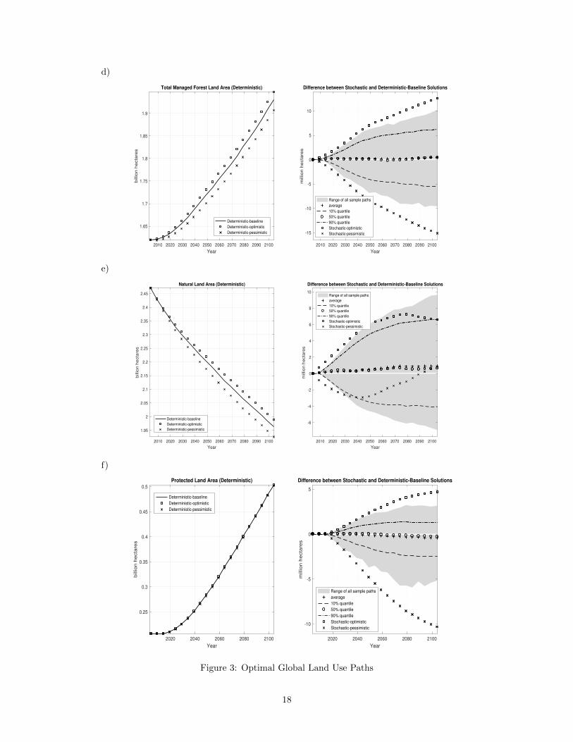
Figure 3 depicts the optimal allocation of global land use over the next century. The
left-hand side of Figure 3 shows the deterministic paths of di↵erent types of land considered
25The model converges to its stationary state around 2150. The di↵erences in land use allocations between2100 and 2150 are small and therefore not reported.
15

in this study, i.e., when the food crop yields are perfectly anticipated. Specifically, it shows
three scenarios, where the value of the crop technology index corresponds to (i) expected val-
ues of the stochastic crop productivity index (deterministic-baseline scenario), (ii) the most
pessimistic climate and bad technology states (deterministic-pessimistic scenario), and (iii)
the most optimistic climate and good technology states (deterministic-optimistic scenario).
The right-hand side of Figure 3 shows the di↵erence range between the 1,000 simulation
paths based on di↵erent ex-ante realizations of the stochastic crop productivity index and
the deterministic-baseline path. The 10%, 50% and 90% quantile lines represent 10%, 50%
and 90% quantiles of 1,000 simulated values respectively at each time, and the average line
(the “+” line) represent the average of 1,000 simulated values respectively at each time.
The right-hand side of Figure 3 also shows two extreme cases of optimal land-use paths
conditional on period t realizations of crop productivity index states At(J1,t, J2,t). The
realized crop productivity index always takes the highest possible value in a stochastic-
optimistic case (the line of squares), and the lowest possible value in a stochastic-pessimistic
case (the line of marks). As future realizations of the stochastic crop productivity index
are uncertain, these extreme stochastic solutions are not the same as the corresponding
deterministic solutions, where the values of future crop productivity index are known with
certainty. In the stochastic-optimistic case, for example, potentially lower realizations of
future crop productivity index result in larger current-period agricultural land allocation
as compared to the deterministic-optimistic solution. For other model variables, due to
resource limits (e.g., the total land area is unchanged over time) and other constraints, the
impact of uncertainty is theoretically di�cult to assess.
We start with the left-hand side of panels (a)-(e) of Figure 3 that shows the optimal
land use paths under the perfect foresight. Beginning with the description of the baseline
scenario we see that, in the first half of the coming century, the area dedicated to food crops
increases by 350 million hectares or 22 percent compared to 2004, reaching its maximum of
1.88 billion hectares around mid-century (panel a). Continuing population growth, intensi-
fication of livestock production, and increasing demand for food, stemming from economic
growth are the key drivers for this cropland expansion. In the second half of the coming
century, slower population growth, and technology improvements in crop yields and food
processing result in a smaller demand for cropland. By 2100 cropland area declines signifi-
cantly relative to its peak value, falling to 1.45 billion hectares, which is, 6 percent smaller
than in 2004. In the first half of the coming century land allocation for the second-generation
biofuels is close to zero (panel b). Consistent with the recent analysis of 2G biofuels’ deploy-
ment potential (National Research Council, 2011), absent aggressive GHG regulations and
biofuels’ policies, this technology is suboptimal because of low extraction and refining costs
of fossil fuels and high production and deployment costs of the second-generation biofuels.
In the second half of the coming century, the second-generation technology becomes viable,
as fossil fuels become scarce and costs of producing the second-generation biofuels decline.
This results in greater land requirements for the second-generation biofuels crops. By the
end of the coming century, agricultural land dedicated to the second-generation biofuels
crops adds 500 million hectares. Consistent with recent trends, global pasture area declines
throughout the entire century (panel c), reflecting increased substitution of pasture land for
16

a)
2010 2020 2030 2040 2050 2060 2070 2080 2090 2100
Year
1.4
1.5
1.6
1.7
1.8
1.9
bill
ion
he
cta
res
Agricultural Land Area, Food Crops (Deterministic)
Deterministic-baseline
Deterministic-optimistic
Deterministic-pessimistic
Difference between Stochastic and Deterministic-Baseline Solutions
2010 2020 2030 2040 2050 2060 2070 2080 2090 2100
Year
-80
-60
-40
-20
0
20
40
60
80
100
mill
ion
he
cta
res
Range of all sample paths
average
10% quantile
50% quantile
90% quantile
Stochastic-optimistic
Stochastic-pessimistic
b)
2010 2020 2030 2040 2050 2060 2070 2080 2090 2100
Year
0.05
0.1
0.15
0.2
0.25
0.3
0.35
0.4
0.45
0.5
0.55
billio
n h
ecta
res
Agricultural Land Area, 2G Biofuels Crops (Deterministic)
Deterministic-baseline
Deterministic-optimistic
Deterministic-pessimistic
Difference between Stochastic and Deterministic-Baseline Solutions
2010 2020 2030 2040 2050 2060 2070 2080 2090 2100
Year
-100
-80
-60
-40
-20
0
20
40
60
80
millio
n h
ecta
res
Range of all sample paths
average
10% quantile
50% quantile
90% quantile
Stochastic-optimistic
Stochastic-pessimistic
c)
2010 2020 2030 2040 2050 2060 2070 2080 2090 2100
Year
2.2
2.25
2.3
2.35
2.4
2.45
2.5
2.55
2.6
2.65
2.7
bill
ion
he
cta
res
Pasture Land Area (Deterministic)
Deterministic-baseline
Deterministic-optimistic
Deterministic-pessimistic
Difference between Stochastic and Deterministic-Baseline Solutions
2010 2020 2030 2040 2050 2060 2070 2080 2090 2100
Year
-4
-2
0
2
4
6
mill
ion
he
cta
res
Range of all sample paths
average
10% quantile
50% quantile
90% quantile
Stochastic-optimistic
Stochastic-pessimistic
17
d)
2010 2020 2030 2040 2050 2060 2070 2080 2090 2100
Year
1.65
1.7
1.75
1.8
1.85
1.9
bill
ion h
ecta
res
Total Managed Forest Land Area (Deterministic)
Deterministic-baseline
Deterministic-optimistic
Deterministic-pessimistic
Difference between Stochastic and Deterministic-Baseline Solutions
2010 2020 2030 2040 2050 2060 2070 2080 2090 2100
Year
-15
-10
-5
0
5
10
mill
ion h
ecta
res
Range of all sample paths
average
10% quantile
50% quantile
90% quantile
Stochastic-optimistic
Stochastic-pessimistic
e)
2010 2020 2030 2040 2050 2060 2070 2080 2090 2100
Year
1.95
2
2.05
2.1
2.15
2.2
2.25
2.3
2.35
2.4
2.45
bill
ion
he
cta
res
Natural Land Area (Deterministic)
Deterministic-baseline
Deterministic-optimistic
Deterministic-pessimistic
Difference between Stochastic and Deterministic-Baseline Solutions
2010 2020 2030 2040 2050 2060 2070 2080 2090 2100
Year
-6
-4
-2
0
2
4
6
8
10
mill
ion
he
cta
res
Range of all sample paths
average
10% quantile
50% quantile
90% quantile
Stochastic-optimistic
Stochastic-pessimistic
f)
2020 2040 2060 2080 2100
Year
0.25
0.3
0.35
0.4
0.45
0.5
billio
n h
ecta
res
Protected Land Area (Deterministic)
Deterministic-baseline
Deterministic-optimistic
Deterministic-pessimistic
Difference between Stochastic and Deterministic-Baseline Solutions
2020 2040 2060 2080 2100
Year
-10
-5
0
5
millio
n h
ecta
res
Range of all sample paths
average
10% quantile
50% quantile
90% quantile
Stochastic-optimistic
Stochastic-pessimistic
Figure 3: Optimal Global Land Use Paths
18
animal feed in livestock production (Taheripour et al., 2013). Managed forest area increases
throughout the entire century reaching 1.95 billion Ha by 2100 (panel d). In contrast, in
response to greater requirements for agricultural land, unmanaged forest area declines by
about 500 million Ha over the course of the 21st century (panel e). The decline in unman-
aged forest land is less environmentally damaging in the second half of the coming century,
as deforestation is limited, with most of the unmanaged forests being converted to managed
or protected forest land. Finally, protected forest area more than doubles by the end of the
coming century, in light of strong growth in the demand for ecosystem services (panel f).
The other two scenarios exhibit broadly similar dynamics. As expected, compared to the
baseline scenario, the most pessimistic scenario foresees a greater expansion of agricultural
land for food crops and reduction in other types of land (except for protected lands) in re-
sponse to expected lower realizations of the crop technology index. The situation is reversed
for the optimistic scenario. There is a significant variation in the range of anticipated ex-
pansion of the agricultural area for food crops between optimistic and pessimistic scenarios,
which amounts to 200 million hectares or 14 percent of total cropland in 2100. Variation
in expected land use change for other types of land accounts for an approximately equal
proportion of the variation in agricultural land for food crops, whereas protected forest areas
change very little across di↵erent climate scenarios.
Uncertainty in the crop productivity index results in additional redistribution of land
resources so to o↵set the impact of potentially lower yields. As social preferences exhibit
intertemporal substitution in this stochastic application of the FABLE model, some of that
redistribution takes place even in the absence of the actual changes in the states of climate
or technology.26 Compared to the deterministic scenario, the median (i.e., the 50 percent
quantile) path of global land use that correspond to the “medium” state of climate (J1,t = 3)
and the “medium” technological state (J2,t = 2) foresees a smaller use of agricultural land
for food crops (panel a), and greater use of agricultural land for 2G, biofuels’ crops (panel
b), pasture land (panel c), managed forest land (panel d). There is also a decline in the
protected land area (panel e) and an increase in unmanaged natural land (panel d). Unlike
the deterministic scenario, almost all of the variation in global land resources in stochastic
simulations happens across agricultural land for food crops and 2G biofuels crops (panels
a and b). For all other land resources, the di↵erences between stochastic and deterministic
paths are small and economically insignificant. This is because land conversion costs of
agricultural land for other types of land become larger in the presence of uncertainty. These
other types of land have higher adjustment costs of conversion associated with additional
time cost of regrowing lumber and livestock, and irreversibilities in accessing protected land
areas. Land rotation between food crops and 2G biofuels crops is less costly in the FABLE
model. This result is consistent with earlier studies that find that closer integration with the
energy sector o↵ers greater potential for food-energy substitution, and thus also a greater
resilience against adverse climate conditions a↵ecting food crop yields (Di↵enbaugh et al.,
2012; Verma et al., 2014).
While the direction of the e↵ect of the uncertainty in the crop productivity on land
26 This result is similar to the theoretical findings and numerical simulations of Lanz et al. (2017).
19

conversion can be inferred from the economic theory of environmental and natural resource
management under uncertainty (see, e.g., Tsur and Zemel (2014) and references therein), the
extent to which this uncertainty propagates into land conversion depends critically on chosen
model structure and parameters. For example, Alexander et al. (2017, p.1) find that even in
the absence of intrinsic uncertainty “systematic di↵erences in land cover areas are associated
with the characteristics modeling approach are at least as great as the di↵erences attributed
to scenario variations”. Depending on the assumptions on the substitution of land for other
resources, the size of technological progress, and the responsiveness of demand for land-based
goods and services to changes in the crop productivity, this magnitude can be substantially
di↵erent for other land use models. However, for the same model parameters, we can
see that the range of land conversion is considerably smaller for the dynamic stochastic
model as compared to the deterministic scenario analysis. As we see from Figure 3, panel
(a), the di↵erence between the most extreme paths of the stochastic crop productivity
index is about 170 million hectares at 2100 or about 12 percent of the total agricultural
area dedicated to food crops. About half of that variation can be attributed to the most
extreme (i.e., falling beyond 10th and above 90th percent quantiles) realizations of crop
productivity. This is because the stochastic model assumes that climate and technological
states a↵ecting crop yields are reversible (that is, if the current state is “bad” (or “good”),
it could be “good” (or “bad”) in future). In comparison with the deterministic model under
the pessimistic (or optimistic) scenario, the social optimum in the stochastic model requires
smaller (or greater) conversion of other types of land to cropland. Thus, agricultural land
area in the deterministic pessimistic (or optimistic) scenario is larger (or smaller) than the
largest (or the smallest) path in the stochastic simulations. For example, in 2100, under the
deterministic-pessimistic scenario, the cropland deviation from the deterministic-baseline
scenario is about 100 million hectares, which is 25 percent larger than the largest deviation
under the stochastic simulations, and about twice as large than the deviation above the 90%
quantile of the stochastic crop technology index. This result demonstrates that scenario
analysis can significantly overstate the magnitude of expected agricultural land conversion
under uncertain crop yields.
5.2 Optimal Path of Land-Based Goods and Services under Crop
Yield Uncertainty
The left-hand side panels of Figure 4 report the optimal paths of land-based goods and
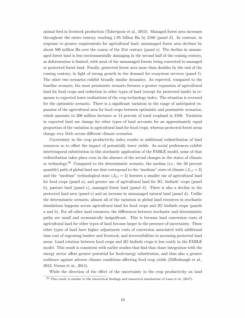
services under the deterministic model scenarios. Beginning with the baseline scenario, the
first panel of Figure 4 shows the production path of food crops, which increases steadily in
the first half of the coming century. Compared to 2004, production of food crops (including
livestock and biofuels feedstock) nearly doubles, reaching its maximum of about 11 billion
tons around 2050. As with cropland expansion, rapid population growth and rising incomes
are the key drivers for growing consumption on the demand side. On the supply side, the
increase in the production of food crops is further boosted by growing crop yields. At the
end of the coming century, production of food crops moderates, as consumers satiate their
food requirements and the technology of food marketing and processing improves. By 2100
crop production for the livestock feed has leveled o↵ and even begins to decline. There is also
20

a)
2010 2020 2030 2040 2050 2060 2070 2080 2090 2100
Year
7
8
9
10
11
12
bill
ion
to
ns
Food Crops (Deterministic)
Deterministic-baseline
Deterministic-optimistic
Deterministic-pessimistic
Difference between Stochastic and Deterministic-Baseline Solutions
2010 2020 2030 2040 2050 2060 2070 2080 2090 2100
Year
-3
-2
-1
0
1
2
bill
ion
to
ns
Range of all sample paths
average
10% quantile
50% quantile
90% quantile
Stochastic-optimistic
Stochastic-pessimistic
b)
2010 2020 2030 2040 2050 2060 2070 2080 2090 2100
Year
5
10
15
20
25
30
35
million tonnes o
f oil e
quiv
ale
nt
Biofuels (Deterministic)
Deterministic-baseline
Deterministic-optimistic
Deterministic-pessimistic
Difference between Stochastic and Deterministic-Baseline Solutions
2010 2020 2030 2040 2050 2060 2070 2080 2090 2100
Year
-10
-5
0
5
10
15
20m
illion tonnes o
f oil e
quiv
ale
nt
Range of all sample paths
average
10% quantile
50% quantile
90% quantile
Stochastic-optimistic
Stochastic-pessimistic
c)
2010 2020 2030 2040 2050 2060 2070 2080 2090 2100
Year
200
400
600
800
1000
1200
1400
1600
millio
n t
on
ne
s o
f o
il e
qu
iva
len
t
2G Biofuels (Deterministic)
Deterministic-baseline
Deterministic-optimistic
Deterministic-pessimistic
Difference between Stochastic and Deterministic-Baseline Solutions
2010 2020 2030 2040 2050 2060 2070 2080 2090 2100
Year
-300
-250
-200
-150
-100
-50
0
50
100
150
200
millio
n t
on
ne
s o
f o
il e
qu
iva
len
t
Range of all sample paths
average
10% quantile
50% quantile
90% quantile
Stochastic-optimistic
Stochastic-pessimistic
21
d)
2010 2020 2030 2040 2050 2060 2070 2080 2090 2100
Year
0.9
1
1.1
1.2
1.3
1.4
1.5
bill
ion
to
ns
Livestock (Deterministic)
Deterministic-baseline
Deterministic-optimistic
Deterministic-pessimistic
Difference between Stochastic and Deterministic-Baseline Solutions
2010 2020 2030 2040 2050 2060 2070 2080 2090 2100
Year
-300
-200
-100
0
100
200
mill
ion
to
ns
Range of all sample paths
average
10% quantile
50% quantile
90% quantile
Stochastic-optimistic
Stochastic-pessimistic
e)
2010 2020 2030 2040 2050 2060 2070 2080 2090 2100
Year
1.6
1.8
2
2.2
2.4
2.6
2.8
3
3.2
bill
ion
to
ns
Timber (Deterministic)
Deterministic-baseline
Deterministic-optimistic
Deterministic-pessimistic
Difference between Stochastic and Deterministic-Baseline Solutions
2010 2020 2030 2040 2050 2060 2070 2080 2090 2100
Year
-50
-40
-30
-20
-10
0
10
20
30
40
mill
ion
to
ns
Range of all sample paths
average
10% quantile
50% quantile
90% quantile
Stochastic-optimistic
Stochastic-pessimistic
f)
2010 2020 2030 2040 2050 2060 2070 2080 2090 2100
Year
2.3
2.4
2.5
2.6
2.7
2.8
2.9
3
billion U
SD
Output of Ecosystem Services (Deterministic)
Deterministic-baseline
Deterministic-optimistic
Deterministic-pessimistic
Difference between Stochastic and Deterministic-Baseline Solutions
2010 2020 2030 2040 2050 2060 2070 2080 2090 2100
Year
-30
-25
-20
-15
-10
-5
0
5
10
15
20
million o
f 2004 U
S d
ollars
Range of all sample paths
average
10% quantile
50% quantile
90% quantile
Stochastic-optimistic
Stochastic-pessimistic
Figure 4: Optimal Paths of Land-Based Goods and Services
22
a significant variation in the range of production of food crops between the most optimistic
and pessimistic scenarios, which amounts to the sizable amount of 5.3 billion tons.
The results of the dynamic stochastic model simulations also show that uncertainty
in the crop productivity index has a profound e↵ect on the optimal production path of
food crops. Between the most extreme paths of the stochastic crop productivity index,
production of food crops varies by about 5.4 billion tons compared to the corresponding
deterministic path of the stochastic crop productivity index. This is a sizable change, which
suggests a significant variation in levels of consumption in 2100 along di↵erent paths of
stochastic crop productivity index. In the FABLE model, much of the variation in the
optimal path of food crops come on the demand side, with the crop productivity decline
resulting primarily in the reduced consumption of processed crops and livestock. As shown
above, the uncertainty-induced supply response is relatively small along the extensive margin
in the dynamic stochastic model (i.e., land conversion). In the online appendix (Figure C.1,
panel a) we show that the supply response on the intensive margin is smaller, with the ratio
of fertilizers to cropland increasing by less than 6 kg/Ha (or eight percent) under extreme
realizations of climate and technology uncertainties. About a half of that di↵erence, however,
corresponds to the most extreme (i.e., falling beyond 10th and above 90th percent quantiles)
realizations of crop productivity. This result indicates that extreme uncertainty in crop
productivity could have a significant impact on food consumption over the coming century.
Production of both first- and second- generation biofuels in the deterministic model
grows as oil becomes scarcer along the baseline path and agricultural yields increase (panels
b and c). Along that optimal path, characterized by the absence of climate and renewables
policies and the abundance of cheap fossil fuels in the first part of the coming century, first-
generation biofuels never become a large source of energy consumption. In 2100 production
of first- generation biofuels is a mere 20 million tonnes of oil equivalent (Mtoe) in the
baseline scenario, and 40 Mtoe in the optimistic scenario. These numbers are considerably
higher compared to 2004 but are still small in relative terms (less than one percent of
total liquid fuel consumption: see technical appendix, Figure C.1, panel b). In contrast,
the production of second-generation biofuels takes o↵ sharply and expands rapidly after
2040 as they become cost-competitive relative to increasingly costly fossil fuels. In 2100
production of second-generation biofuels reaches 1.55 billion tonnes of oil equivalent (Btoe)
in the baseline scenario. Uncertainty in food crop yields has important implications for the
production of the first-generation biofuels that are directly a↵ected by both climate and
technology states of food crop yields. The di↵erence between the best and worst states of
the crop productivity index is about 31 million tons of oil equivalent, which exceeds their
expected baseline production in 2100. Although climate and technology states of food crop
yields do not directly a↵ect yields of the second- generation biofuels crops, production of
second-generation biofuels is nonetheless a↵ected through indirect substitution e↵ects of
food for energy in FABLE demand system. There is a sizable variation in the production of
second-generation biofuels between extreme paths of the stochastic crop productivity index,
which accounts for 450 Mtoe, or about 30 percent of their total production in 2100.
Production of livestock in the deterministic model increases throughout the coming cen-
tury (panel d) reflecting shifting diets and the growing demand for processed meat as popula-
23
tion income increases (Foley et al., 2011). By the end of the coming century, the production
of livestock in the baseline scenario increases by about 1.5 times compared to 2004, reaching
1.28 billion tons. Given the important contribution of the livestock feed in the production
of livestock, we can see its production is smaller in the pessimistic scenario and larger in the
optimistic scenario. The di↵erence in livestock production between the optimistic and pes-
simistic scenarios accounts for about 550 million tons. This range is similar to the dynamic
stochastic model. As the significance of animal feed in livestock production grows over time,
the e↵ect of uncertain crop yields becomes more pronounced. Similar to the result for food
crops, the most extreme paths of crop productivity account for about a third of all variation
in livestock production.
Production of timber in the deterministic model also expands with the growing demand
for timber products and further improvements in forest yields (panel e). By 2100, production
of merchantable timber crops reaches 3.2 billion tons in the deterministic baseline scenario,
which is twice as large as in 2004. The consumption of ecosystem services declines in the near
decades, as unmanaged natural forest lands are converted to croplands (panel f). It then
increases throughout the remaining part of the coming century as the demand for ecosystem
services increases, and more natural forest lands become institutionally protected. By 2100
consumption of ecosystem services is 36 percent larger than in 2004. Crop productivity has
a very small e↵ect on consumption paths of merchantable timber and ecosystem services
in either deterministic or stochastic models. This result is not very surprising as the crop
productivity does not directly a↵ect the production of either timber or ecosystem services,
whereas indirect land use change e↵ects are relatively small in this stochastic application of
the FABLE model.
6 Conclusions
This paper demonstrates how the uncertainties associated with nonstationary biophysi-
cal processes and technological change can be incorporated into an economic analysis of the
optimal allocation of natural resources in the long run. In doing so, it introduces a novel com-
putational method, ENLCEQ, for solving nonstationary dynamic high-dimensional stochas-
tic problems and applies it to FABLE, a recently developed multi-sectoral dynamic model
of global land use.
For illustrative purposes, the study focuses on uncertainty in future crop yields, one of
the core uncertainties a↵ecting the evolution of global land use in the long run. Combining
scenarios from global climate models and high-resolution output from spatial crop simulation
models for four major crops, it comes up with a plausible range of realizations of climate
shocks and their e↵ect on future crop yields. These estimates are supplemented with an
extensive survey of recent agro-economic and biophysical studies assessing the potential for
closing yield gaps as well as attaining further advances in potential yields through plant
breeding.
The paper’s key insight is to illustrate the magnitude of optimal land conversion deci-
sions in the context of di↵erent realizations of the stochastic crop productivity. Consistent
with the economic theory of natural resource management under uncertainty, the agricul-
tural productivity shocks, due either to adverse climate impacts or unexpected limits on
24

further technological progress, result in additional conversion of scarceland resource to o↵-
set the impact of potentially lower yields. Owing to intertemporal substitution, some of
that conversion takes place even in the absence of actual realization of the climate shocks or
technology outcomes. This expansion is accompanied by the changes in the consumption of
processed food, livestock, and biofuels - the land-based products most a↵ected by changes
in crop productivity.
This study is primarily a methodological contribution, and the chosen model illustration
(FABLE) seeks to balance computational complexity and economic tractability. It thus
ignores many features standard in more advanced computational land and other resource
use models. The future research should focus on integrating economic decisions under
uncertainty into large dynamic natural resource models that feature spatial disaggregation at
the regional or zonal level, a more extensive representation of the energy sector, and di↵erent
types of resources and their production derivatives. Another promising research direction
would be to incorporate a more detailed representation of uncertain states backed by an
econometric analysis that recovers underlying distributions of uncertain natural resource
drivers over time.
References
Alexander, P., R. Prestele, P. H. Verburg, A. Arneth, C. Baranzelli, F. Batista e Silva,
C. Brown, A. Butler, K. Calvin, N. Dendoncker, et al. (2017). Assessing Uncertainties in
Land Cover Projections. Global Change Biology 23 (2), 767–781.
Babiker, M., A. Gurgel, S. Paltsev, and J. Reilly (2009). Forward-looking versus Recursive-
dynamic Modeling in Climate Policy Analysis: A Comparison. Economic Modelling 26 (6),
1341–1354.
Benayas, J., A. Newton, A. Diaz, and J. Bullock (2009). Enhancement of Biodiversity
and Ecosystem Services by Ecological Restoration: a Meta-analysis. Science 325 (5944),
1121–1124.
Brock, W. A. and M. Majumdar (1978). Global Asymptotic Stability Results for Multisec-
tor Models of Optimal Growth under Uncertainty when Future Utilities are Discounted.
Journal of Economic Theory 18 (2), 225–243.
Bulte, E., D. van Soest, G. Van Kooten, and R. Schipper (2002). Forest Conservation
in Costa Rica when Nonuse Benefits are Uncertain but Rising. American Journal of
Agricultural Economics 84 (1), 150–160.
Burke, M. B. and K. Emerick (2016). Adaptation to Climate Change: Evidence from US
Agriculture. American Economic Journal: Economic Policy 8 (3), 106–140.
Cai, Y. (2019). Computational methods in environmental and resource economics. Annual
Review of Resource Economics (11), 59–82.
Cai, Y. and K. Judd (2013). Shape-preserving Dynamic Programming. Mathematical Meth-
ods of Operations Research 77 (3), 407–421.
25
Cai, Y. and K. Judd (2014). Advances in Numerical Dynamic Programming and New
Applications. In K. L. Judd and K. Schmedders (Eds.), Handbook of Computational
Economics. Elsevier.
Cai, Y., K. Judd, and J. Steinbuks (2017). A Nonlinear Certainty Equivalent Approximation
Method for Dynamic Stochastic Problems. Quantitative Economics 8 (1), 117–147.
Cai, Y., K. Judd, G. Thain, and S. Wright (2015). Solving Dynamic Programming Problems
on a Computational Grid. Computational Economics 45 (2), 261–284.
Cai, Y. and T. Lontzek (2019). The social cost of carbon with economic and climate risks.
Journal of Political Economy 127 (6), 2684–2734.
Cassman, K., P. Grassini, and J. van Wart (2010). Crop Yield Potential, Yield Trends,
and Global Food Security in a Changing Climate. In D. Hillel and C. Rosenzweig (Eds.),
Handbook of Climate Change and Agroecosystems, pp. 37–51. Imperial College Press.
Cassman, K. G. (1999). Ecological Intensification of Cereal Production Systems: Yield
Potential, Soil Quality, and Precision Agriculture. Proceedings of the National Academy
of Sciences 96 (11), 5952–5959.
Chazdon, R. (2008). Beyond Deforestation: Restoring Forests and Ecosystem Services on
Degraded Lands. Science 320 (5882), 1458–1460.
Conrad, J. (1997). On the Option Value of Old-growth Forest. Ecological Economics 22 (2),
97–102.
Conrad, J. (2000). Wilderness: Options to Preserve, Extract, or Develop. Resource and
Energy Economics 22 (3), 205–219.
Daigneault, A. J., M. J. Miranda, and B. Sohngen (2010). Optimal Forest Management
with Carbon Sequestration Credits and Endogenous Fire Risk. Land Economics 86 (1),
155–172.
Den Haan, W. J., K. L. Judd, and M. Juillard (2011). Computational Suite of Models
with Heterogeneous Agents II: Multi-country Real Business Cycle Models. Journal of
Economic Dynamics and Control 35 (2), 175–177.
Di↵enbaugh, N. S., T. W. Hertel, M. Scherer, and M. Verma (2012). Response of Corn Mar-
kets to Climate Volatility under Alternative Energy Futures. Nature climate change 2 (7),
514.
Drud, A. S. (1994). CONOPT?A Large-Scale GRG Code. ORSA Journal on Comput-
ing 6 (2), 207–216.
Evans, L. and R. Fischer (1999). Yield Potential: its Definition, Measurement, and Signifi-
cance. Crop Science 39 (6), 1544–1551.
Foley, J. A., N. Ramankutty, K. A. Brauman, E. S. Cassidy, J. S. Gerber, M. Johnston, N. D.
Mueller, C. O’Connell, D. K. Ray, P. C. West, et al. (2011). Solutions for a Cultivated
Planet. Nature 478 (7369), 337–342.
26

Fussel, H.-M. (2009). An Updated Assessment of the Risks from Climate Change Based on
Research Published since the IPCC Fourth Assessment Report. Climatic change 97 (3-4),
469.
Grassini, P., K. M. Eskridge, and K. G. Cassman (2013). Distinguishing between Yield
Advances and Yield Plateaus in Historical Crop Production Trends. Nature Communica-
tions 4.
Hertel, T., S. Rose, and R. Tol (2009). Economic Analysis of Land Use in Global Climate
Change Policy. Routledge.
Hertel, T., J. Steinbuks, and W. Tyner (2016). What is the Social Value of Second Gener-
ation Biofuels? Applied Economic Perspectives and Policy 38 (4), 599–617.
Hertel, T. W., J. Steinbuks, and U. Baldos (2013). Competition for Land in the Global
Bioeconomy. Agricultural Economics 44 (s1), 129–138.
IPCC (2014a). Climate Change 2014: Impacts, Adaptation and Vulnerability: Contribution
of Working Group II to the Fifth Assessment Report of the Intergovernmental Panel on
Climate Change. Cambridge University Press.
IPCC (2014b). Climate Change 2014: Impacts, Adaptation and Vulnerability: Contribution
of Working Group III to the Fifth Assessment Report of the Intergovernmental Panel on
Climate Change. Cambridge University Press.
Judd, K. L. (1998). Numerical Methods in Economics. The MIT press.
Kumar, P. (2010). The Economics of Ecosystems and Biodiversity: Ecological and Economic
Foundations. Routledge.
Lanz, B., S. Dietz, and T. Swanson (2017). Global Economic Growth and Agricultural
Land Conversion under Uncertain Productivity Improvements in Agriculture. American
Journal of Agricultural Economics 100 (2), 545–569.
Leroux, A., V. Martin, and T. Goeschl (2009). Optimal Conservation, Extinction Debt, and
the Augmented Quasi-option Value. Journal of Environmental Economics and Manage-
ment 58 (1), 43–57.
Licker, R., M. Johnston, J. A. Foley, C. Barford, C. J. Kucharik, C. Monfreda, and N. Ra-
mankutty (2010). Mind the Gap: How do Climate and Agricultural Management Explain
the ’Yield Gap’ of Croplands around the World? Global Ecology and Biogeography 19 (6),
769–782.
Lobell, D. B., K. G. Cassman, and C. B. Field (2009). Crop Yield Gaps: their Importance,
Magnitudes, and Causes. Annual Review of Environment and Resources 34 (1), 179.
Lobell, D. B. and C. B. Field (2007). Global Scale Climate - Crop Yield Relationships and
the Impacts of Recent Warming. Environmental Research Letters 2 (1), 014002.
Majumdar, M. and R. Radner (1983). Stationary Optimal Policies with Discounting in a
Stochastic Activity Analysis Model. Econometrica 51 (6), 1821–1837.
27
Miranda, M. J. and P. L. Fackler (2004). Applied Computational Economics and Finance.
MIT press.
National Research Council (2011). Renewable Fuel Standard: Potential Economic and En-
vironmental E↵ects of U.S. Biofuel Policy. National Academies Press.
Nesshover, C., J. Aronson, J. Blignaut, D. Lehr, A. Vakrou, and H. Wittmer (2009). In-
vesting in Ecological Infrastructure. In P. ten Brink (Ed.), The Economics of Ecosystems
and Biodiversity: National and International Policy Making. An Output of TEEB, pp.
401–448. Earthscan.
Nikas, A., H. Doukas, and A. Papandreou (2019). A Detailed Overview and Consistent
Classification of Climate-Economy Models. In Understanding Risks and Uncertainties in
Energy and Climate Policy, pp. 1–54. Springer.
Pindyck, R. S. (1984). Uncertainty in the Theory of Renewable Resource Markets. The
Review of Economic Studies 51 (2), 289–303.
Pindyck, R. S. (2007). Uncertainty in Environmental Economics. Review of Environmental
Economics and Policy 1 (1), 45–65.
Rosenzweig, C., J. Elliott, D. Deryng, A. Ruane, A. Arneth, K. Bootef, C. Folberth, M. Glot-
ter, N. Khabarov, C. Muller, K. Neumann, F. Piontek, T. Pugh, E. Schmid, E. Stehfest,
and J. Jones (2014). Assessing Agricultural Risks of Climate Change in the 21st Century
in a Global Gridded Crop Model Intercomparison. Proceedings of the National Academy
of Sciences 111 (9), 3268–3273.
Schmitz, C., H. van Meijl, P. Kyle, G. C. Nelson, S. Fujimori, A. Gurgel, P. Havlik, E. Hey-
hoe, D. M. d’Croz, A. Popp, et al. (2014). Land-Use Change Trajectories Up to 2050:
Insights from a Global Agro-Economic Model Comparison. Agricultural Economics 45 (1),
69–84.
Sohngen, B. and R. Mendelsohn (2003). An Optimal Control Model of Forest Carbon
Sequestration. American Journal of Agricultural Economics 85 (2), 448–457.
Sohngen, B. and R. Mendelsohn (2007). A Sensitivity Analysis of Forest Carbon Seques-
tration. In M. Schlesinger (Ed.), Human-Induced Climate Change: An Interdisciplinary
Assessment, pp. 227–237. Cambridge University Press.
Steinbuks, J. and T. Hertel (2012). Forest, Agriculture, and Biofuels in a Land use model
with Environmental services (FABLE). GTAPWorking Paper 71, Center for Global Trade
Analysis, Department of Agricultural Economics, Purdue University.
Steinbuks, J. and T. Hertel (2016). Confronting the Food-Energy-Environment Trilemma:
Global Land Use in the Long Run. Environmental and Resource Economics 63 (3), 545–
570.
Steinbuks, J. and T. W. Hertel (2013). Energy Prices Will Play an Important Role in
Determining Global Land Use in the Twenty First Century. Environmental Research
Letters 8 (1), 014014.
28
Stokey, N. L., R. E. Lucas, and E. C. Prescott (1989). Recursive Methods in Economic
Dynamics. Harvard University Press.
Taheripour, F., C. Hurt, and W. E. Tyner (2013). Livestock Industry in Transition: Eco-
nomic, Demographic, and Biofuel Drivers. Animal Frontiers 3 (2), 38–46.
Tian, X., B. Sohngen, J. B. Kim, S. Ohrel, and J. Cole (2016). Global Climate Change
Impacts on Forests and Markets. Environmental Research Letters 11 (3), 035011.
Tsionas, E. G. and S. C. Kumbhakar (2004). Markov Switching Stochastic Frontier Model.
The Econometrics Journal 7 (2), 398–425.
Tsur, Y. and A. Zemel (2014). Dynamic and Stochastic Analysis of Environmental and
Natural Resources. In M. Fischer and P. Nijkamp (Eds.), Handbook of Regional Science,
pp. 929–949. Springer-Verlag Berlin Heidelberg.
Verma, M., T. Hertel, and N. Di↵enbaugh (2014). Market-Oriented Ethanol and Corn-Trade
Policies can Reduce Climate-Induced US Corn Price Volatility. Environmental Research
Letters 9 (6), 064028.
29
Technical Appendix
A.1 FABLE Model Description
This section and the following section describe key elements of FABLE model,
as well as its equations, variables, and model parameters. For a full descrip-
tion of the model, including details on model baseline calibration and extensive
sensitivity analysis, please refer to Hertel et al. (2016) and Steinbuks & Hertel
(2016) and technical appendices therein.
A.1.1 Primary Resources
Primary resources comprise of land, liquid fossil fuels, and other primary inputs,
e.g., labor and capital. The supply of land is fixed and faces competing uses that
are determined endogenously by the model. The flow of liquid fossil fuels evolves
endogenously along their optimal extraction path, accounting for exogenous
discoveries in new fossil fuel reserves. The endowment of other primary inputs
is exogenous and evolves along the prespecified global economy growth path.
A.1.1.1 Land
The total land endowment in the model, Ltotal, is fixed. Each period of time t
there are four profiles of land in the economy. They include unmanaged forest
land, LN , agricultural land, LA, pasture land, LP , and commercially managed
forest land, LC . The agricultural land area can be allocated for the cultiva-
tion of food crops (denoted LA,c), and second-generation biofuels feedstocks
(denoted LA,b2). We assume that the natural forest land consists of two types.
Institutionally protected land, LR, includes natural parks, biodiversity reserves
and other types of protected forests. This land is used to produce ecosystem
services for society, and cannot be converted to commercial land. Unmanaged
natural land, LN , can be accessed and either converted to managed land or to
protected natural land. Once the natural land is converted to managed land,
its potential to yield ecosystem services is diminished. This potential can be
partially restored for managed forests with significant land rehabilitation costs
incurred. The use of managed land can be shifted between cropland, forestland,
and pasture land (see Figure 1 in the main manuscript for a graphical represen-
tation of these transitions). We denote land transition flows from land type i
1
to land type j as �i,j (a negative value means a transition from land type j to
land type i). Equations describing allocation of land across time and di↵erent
uses are as follows :
Ltotal =X
i=A,P,C,N,R
Lit (A.1)
LA = LA,c + LA,b2 (A.2)
LNt+1 = LN
t ��N,At ��N,R
t +�C,Nt (A.3)
LAt+1 = LA
t +�N,At ��A,P
t +�C,At (A.4)
LPt+1 = LP
t +�A,Pt (A.5)
LRt+1 = LR
t +�N,Rt (A.6)
Equations (A.1) and (A.2) define, respectively, the composition of total land and
agricultural land in the economy. Equations (A.3)-(A.5) describe the transitions
for unmanaged land, agricultural land, and pasture land.1 Equation (A.6) shows
the growth path of protected natural land.
Accessing the natural lands comes at a cost associated with building roads
and other infrastructure (Golub et al. , 2009). In addition, converting natural
land to reserved land entails additional costs associated with passing legislation
to create new natural parks. We denote the natural land access, rehabilitation,
and protection costs as CN,A,R, CC,N , and CN,R, respectively. There are also
costs of switching between the cropland and the pasture land, denoted as CA,P .
We assume that all these costs are continuous, monotonically increasing, and
strictly convex functions of converted land. There are no additional costs of
natural land conversion to commercial land, as the revenues from deforestation
o↵set these costs.
Managed forests are characterized by vmax vintages of tree species with vin-
tage ages v = 1, ..., vmax. At the end of period t each hectare of managed forest
1Equations (A.2) and (A.4) do not account for the transition from forestry to pastureland. Throughout the past century tropical forests, particularly in the Latin America region,have been extensively converted to the pasture land (Barbier et al. , 1994). However, in theFABLE model, conversion of forest land to pasture is never optimal as cropland has higherproductivity for cattle breeding at the same conversion (stumpage) cost.
2
land, LCv,t, has an average density of tree vintage age v, with the initial alloca-
tion given and denoted by LCv,0. The forest rotation ages and management are
endogenously determined. Each period the managed forest land can be either
planted, harvested, or left to mature. The newly planted trees occupy �C,C
hectares of land, and reach the average age of the first tree vintage next period.
The harvested area of tree vintage age v occupies �C,Hv hectares of forest land.
The di↵erence between the harvested area of all tree vintage ages and the newly
planted area is used for cropland, i.e.,
�C,At =
X
v
�C,Hv,t ��C,C
t
The following equations describe land use of managed forests:
LCt =
vmaxX
v=1
LCv,t, (A.7)
LCv+1,t+1 = LC
v,t ��C,Hv,t , v < vmax � 1 (A.8)
LCvmax,t+1 = LC
vmax,t ��C,Hvmax,t ��C,N
t + LCvmax�1,t ��C,H
vmax�1,t (A.9)
LC1,t+1 = �C,C
t . (A.10)
Equation (A.7) describes the composition of managed forest area across vin-
tages. Equation (A.8) illustrates the harvesting dynamics of forest areas with
the ages vmax � 1 and vmax. Equation (A.10) shows the transition from the
planted area to new forest vintage area.
The average harvesting and planting costs per hectare of new forest planted,
co,H , and co,C , are invariant to scale and are the same across all vintages. Har-
vesting managed forests and conversion of harvested forest land to agricultural
land is subject to additional near term adjustment costs, cH . The specific func-
tional forms of land conversion costs are shown in section C.1, equations (C.34)-
(C.39).
Thus, we have defined the vector of land state variables:
L =�LN , LA, LP , LR, LC
1 , ..., LCvmax
�
and its associated transition laws.
3
A.1.1.2 Fossil Fuels
The initial stock of liquid fossil fuels, XF , is exogenous, and each period
of time t adds a new amount of fossil fuels, �F,D, which reflects exogenous
technological progress in fossil fuel exploration.2 The economy extracts fossil
fuels, which have two competing uses in our partial equilibrium model of land-
use. A part of extracted fossil fuels, �F,nt , is converted to fertilizers that are
further used in the agricultural sector. The remaining amount of fossil fuels,
�F,Et , is combusted to satisfy the demand for energy services. The following
equation describes supply of fossil fuels:
XFt+1 = XF
t ��F,Et ��F,n
t +�F,Dt . (A.11)
The cost of fossil fuels, cF , reflects the expenditures on fossil fuels’ extraction,
refining, transportation and distribution, as well the costs associated with emis-
sions control (e.g., Pigovian taxes) in the non-land-based economy. We assume
that the cost of fossil fuels is a nonlinear quadratic function with accelerating
costs as the stock of fossil fuels depletes (Nordhaus & Boyer, 2000):
cFt = ⇠F1
⇣�F,E
t +�F,nt
⌘2 XF
0 +�F,Dt
XFt +�F,D
t
!, (A.12)
where the parameter ⇠F1 captures the curvature of the liquid fossil fuel cost
function.
A.1.1.3 Other Primary Resources
The initial endowment of all other primary resources in the non-land-based
economy, such as labor, physical and human capital, and materials inputs, XO,
is exogenous in this model. We assume that the growth rate of all other primary
resources is a weighted average of the population growth, which reflects demo-
graphic changes, and the physical capital growth, o,X . The following equation
describes the supply of other primary inputs:
XOt = XO
0
↵o,l ⇧t
⇧0+�1� ↵o,l
� �1 + o,X
�t�, (A.13)
where ⇧t is the economy’s population, and ↵o,l is the share of population growth
to the growth rate of all other primary resources. Other primary inputs can be
2This technological progress comprises of both discoveries on new exploitable oil and gasfields, as well as development of new technologies for extraction of non-conventional fossilfuels.
4
used for the production of land-based goods and services or converted to final
goods and services in the non-land economy. Thus, state variables for resources
other than land are defined as:
X = (XF , XO).
As XO is exogenous and deterministic, it is a degenerated state variable and
not counted as a state variable for model solution purposes.3
A.1.2 Intermediate Inputs
We analyze six intermediate inputs used in the production of land-based
goods and services: petroleum products, fertilizers, crops, biofuels, and raw
timber. Fossil fuels are refined and converted to either petroleum products,
xp, that are further combusted, or to fertilizers, xn, that are used to boost
yields in the agricultural sector. Agricultural land and fertilizers are combined
to grow food crops, xc or 2G biofuels crops, xc,b2. Food crops can be further
converted into processed food and 1G biofuels, xb1, or used as an animal feed,
xc,l. 2G biofuels crops can only be converted into 2G biofuels, xb2. 1G biofuels
substitute imperfectly for liquid fossil fuels in final energy demand, whereas 2G
biofuels and liquid fossil fuels are the perfect substitutes The food crops used
as animal feed and pasture land are combined to produce raw livestock, xl.
Harvesting managed forests yield raw timber, xw, that is further used in timber
processing. The production functions for intermediate inputs can be illustrated
by the following equations
xjt = gj
�F,{E,n}
t , L{A,P}t ,
X
v
�C,Hv,t , xc,{l,b}
!, j = p, n, c, b, l, w. (A.14)
where �F,{E,n}t represents that either �F,E
t or �F,nt is an argument of gj , sim-
ilarly for L{A,P}t and xc,{l,b}. The specific functional forms of gj (·) are shown
in section C.1, equations (C.14)-(C.22).
A.1.3 Final Goods and Services
We consider five per capita land-based services that are consumed in the final
3 It would be, however, counted as a state variable for the model solution purposes if we
assume that the endowment is a stochastic process.
5
demand: services from processed crops, yf , livestock, yl, energy, ye, timber,
yw, and ecosystem services, yr. Processed crops, livestock, and timber are
respectively products of food crops, raw livestock, and timber processing. The
production of energy services combines liquid fossil fuels with the biofuels, and
the resulting mix is further combusted. The ecosystem services are the public
good to society, which captures recreation, biodiversity, and other environmental
goods and services. To close the demand system, we also include other goods
and services, yo, which comprise of consumption of other primary inputs not
spent on the production of land-based goods and services.
We have defined all state variables for the deterministic model:
S := (L,X),
and the vector of decision variables is
at := (�N,At ,�N,R
t ,�C,Nt ,�A,P
t ,�C,At ,�C,H
1,t , ...,�C,Hvmax,t,�
C,Ct ,�F,E
t ,�F,nt , LA,F
t , LA,Bt ,xt,yt),
where xt ⌘ [xpt , x
nt , x
ct , x
bt , x
lt, x
wt , x
c,lt , xc,b
t ] and yt =⇣yft , y
lt, y
et , y
wt , y
rt , y
ot
⌘.
The production functions for final per capita land-based goods and services
can be illustrated by the following equation:
yit = F it (St,at) , i = f, l, e, w, r. (A.15)
where some arguments in F i (·) could be redundant. It follows from equation
(A.15) that production of final goods and services involves the combination of
land resources and intermediate inputs. The specific functional forms of F i (·)are shown in section C.1, equations (C.23)-(C.29), which are functions of L
and {xj}. All these equations constitute a part of the feasibility constraint
at 2 Dt(St).
The production of intermediate inputs or final land-based goods and services
i incurs costs, co,i, that are subtracted from available other primary resources.
The remaining amount of other primary resources is converted into other goods
and services, which are subsequently consumed in final demand. As the focus of
this model is on the utilization of land-based resources, we introduce the other
goods and services, yo, in a very simplified manner. We introduce no additional
cost of producing other goods and services, assuming that it is reflected in the
size of the endowment of other primary inputs. The specific functional form for
yo is shown in section C.1, equation (C.28).
6
A.1.4 Preferences
The economy’s per-capita utility, u, is derived from the per capita consump-
tion of processed crops, livestock, timber, energy and ecosystem services, and
other goods and services. Following the macro economic literature, we assume
constant relative risk aversion utility,
u(y) =C(y)1��
1� �, (A.16)
where is the per capita consumption bundle of goods and services, C(y) is a
nonlinear aggregator over y, and � is the coe�cient of relative risk aversion,
which captures the economy’s attitude to uncertain events. We choose a non-
homothetic AIDADS preference (Rimmer & Powell, 1996) to compute C(y) im-
plicitly:
log (C(y)) =X
q=f,l,e,w,r,o
✓↵q + �qC(y)1 + C(y)
◆log�yq � yq
�(A.17)
where ↵, �, and yq are positive parameters withP
q ↵q =P
q �q = 1. These
preferences place greater value on eco-system services, and smaller value on
additional consumption of food, energy and timber products as society becomes
wealthier. When � = 1, our utility function is equivalent to the AIDADS utility.
A.1.5 Welfare
We denote the transition laws of land, (A.3)-(A.6) and (A.8)-(A.10), as
Lt+1 = GLt (St,at), (A.18)
and the transition laws for other resources, (A.11)-(A.13), as
Xt+1 = GXt (St,at). (A.19)
Combining (A.18) and (A.19), we have
St+1 = Gt(St,at) (A.20)
for the deterministic model in the notations of Section 2.
The objective of the planner is to maximize the total expected welfare, which
is the cumulative expected utility of the population’s consumption of final goods
and services, y, discounted at the constant rate � > 0. The planner allocates
7
managed agricultural, pasture and forest lands for crop, livestock, and timber
production, the scarce fossil fuels and protected natural forests to solve the
following problem:
maxa
1X
t=0
�tU(St,at) (A.21)
subject to the transition laws (A.20) and the feasibility constraints at 2 Dt(St)which
include (A.15), (C.23)-(C.29), (C.28), (A.17) and nonnegativity constraints for
the variables. Here
U(St,at) = u(yt)⇧t
is the utility function in the notations of Section 2.
B.1 Quantifying the Uncertainty in Crop Yields
B.1.1 Uncertainty in Agricultural Technology
Advances in crop technology are very di�cult to predict due to four intercon-
nected factors (Fischer et al. , 2011). First, there is significant uncertainty about
the potential for exploiting large and economically significant yield gaps (i.e., the
di↵erences between observed and potential crop yields) in developing countries,
especially those in Sub-Saharan Africa. A second and closely related point is
that it is unclear how fast available yield-enhancing technologies can be adopted
at a global scale.4 Third, there is a significant variation in developing countries’
institutions and policies that make markets work better and provide a conducive
environment for agricultural technology adoption.5 Finally, while plant breeders
continue to make steady gains in further advancing crop yields, progress depends
on the level of funding provided for agricultural research. This has proven to
be somewhat volatile, with per capita funding falling in the decades leading up
to the recent food crisis (Alston & Pardey, 2014). The food price rises since
2007 have stimulated new investments. However, whether this interest will be
sustained remains to be seen. Overall, progress from conventional breeding is
becoming more di�cult. Transgenic (genetic modification) technologies have a
proven record of more than a decade of safe and environmentally sound use,
and thus o↵er huge potential to address critical biotic and abiotic stresses in
4These technologies include conservation farming approaches based on no-tillage, the ge-netic modification technology revolution, and information and communication technologiesfor more e�cient and precise management of modern inputs.
5These best practices include the adoption of better risk management, market development,rural finance, farmers’ organizations, and the provision of advisory services to farmers.
8

the developing world. However, expected yield gains, costs of further developing
these technologies, and the political acceptance of genetically modified foods are
all highly uncertain.
To quantify the extent to which the advances in crop technology can fur-
ther boost agricultural yields over the next century, we first need to assess the
magnitude of existing yield gaps at the global scale. In a comprehensive study,
Lobell et al. (2009) report a significant variation in the ratios of actual to
potential yields for major food crops across the world, ranging from 0.16 for
tropical lowland maize in Sub-Saharan Africa to 0.95 for wheat in Haryana,
India. For the purposes of this study, we employ the results of Licker et al.
(2010), who conduct comprehensive yield gap analysis using global crop dataset
of harvested areas and yields for 175 crops on a 0.5� geographic grid of the
planet for the year 2000. Using these estimates, we calculate the global yield
gap as the grid-level output-weighted yield gap of the four most important food
crops (wheat, maize, soybeans, and rice). The resulting estimate suggests that
average yields are 53% of potential yields, which is close to the median estimates
by Lobell et al. (2009). As a further robustness check we employ the Decision
Support System for Agrotechnology Transfer (DSSAT) crop simulation model
(Jones et al. , 2003), run globally on a 0.5 degree grid in the parallel System
for Integrating Impacts Models and Sectors (pSIMS; Elliott et al. 2014b) to
simulate yields of the same four major food crops under best agricultural man-
agement conditions and compare simulated yields to their observed yields. The
resulting yield gap estimates were not substantially di↵erent.
In the optimistic (i.e., “good”) state of advances in crop technology, we
assume that yields continue to grow linearly throughout the coming century,
eliminating the yield gap by 2100. This high yield scenario rests on the as-
sumption of continued strong growth in investment in agricultural research and
development, widespread acceptance of genetically modified crops, continuing
institutional reforms in developing countries, and public and private invest-
ments in the dissemination of new technologies. The erosion of any one of these
component assumptions will likely result in a slowing of crop technology im-
provements. And there are some grounds for pessimism. In a comprehensive
statistical analysis of historical crop production trends, Grassini et al. (2013)
note that
“despite the increase in investment in agricultural R&D and educa-
tion [...] the relative rate of yield gain for the major food crops has
9
decreased over time together with evidence of upper yield plateaus
in some of the most productive domains. For example, investment
in R&D in agriculture in China has increased threefold from 1981
to 2000. However, rates of increase in crop yields in China have re-
mained constant in wheat, decreased by 64% in maize as a relative
rate and are negligible in rice. Likewise, despite a 58% increase in
investment in agricultural R&D in the United States from 1981 to
2000 (sum of public and private sectors), the rate of maize yield gain
has remained strongly linear.”
To capture the possibility of much slower technological improvement in the
coming century, we specify two more pessimistic scenarios. In the “medium”
state of technology, rather than closing the yield gap by 2100, average yields
in 2100 are just three-quarters of yield potential at that point in time. In the
“bad” state of technology, there is no technological progress, and the crop yields
stay the same as at the beginning of the coming century. This is the path on
which we begin the simulation in 2004. As previously noted, we then specify
probabilities with which the crop technology index evolves across the di↵erent
states of technology.
B.1.2 Uncertainty in Climate Change Impacts
In addition to crop technology uncertainty, there is great uncertainty about
the physical environment in which this technology will be deployed. In partic-
ular, long-run changes in both temperature and precipitation are likely to have
an important impact on the productivity of land in agriculture (IPCC, 2014),
and therefore, the global pattern of land use. Quantification of the impact of
climate change on agricultural yields requires coming to grips with three inter-
connected factors (Alexandratos, 2011). First, there is significant uncertainty in
future GHG concentrations along the long-run growth path of the global econ-
omy. Second, the General Circulation Models (GCMs) developed by climate
scientists to translate these uncertain GHG concentrations into climate out-
comes disagree about the spatially disaggregated deviations of temperature and
precipitation from baseline levels. Finally, there is significant uncertainty in the
biophysical models used to determine how changes in temperature and precip-
itation will a↵ect plant growth and the productivity of agriculture in di↵erent
10

agro-ecological conditions. The impact of climate change on food crop yields
depends critically on their phenological development, which, in turn, depends
on the accumulation of heat units, typically measured as growing degree days
(GDDs). More rapid accumulation of GDDs as a result of the climate change
speeds up phenological development, thereby shortening key growth stages, such
as the grain filling stage, hence reducing potential yields (Long, 1991). How-
ever, rising concentrations of CO2 in the atmosphere result in an increase in
potential yields due to improved water use e�ciency, often dubbed the “CO2
fertilization e↵ect” (Long et al. , 2006). Sorting out the relative importance of
these e↵ects and achieving greater confidence in evaluations of climate impacts
on agricultural yields remains an important research question in the agronomic
literature (Cassman et al. , 2010; Rosenzweig et al. , 2014).
To quantify the uncertainty in climate impacts on agricultural yields we
follow the approach of Rosenzweig et al. (2014), who have recently conducted
a globally consistent, protocol-based, multi-model climate change assessment
for major crops with the explicit characterization of uncertainty. To quantify
the uncertainty of impacts of temperature increases due to climate change on
potential crop yields we obtain results of four crop simulation models: GEPIC
(Liu et al. , 2007), LPJmL (Bondeau et al. , 2007), pDSSAT (Jones et al. ,
2003), and PEGASUS (Deryng et al. , 2011).6 All models are run globally
on a 0.5� grid over the period between 1971 and 2099 and weighted by the
agricultural output of four major food crops (maize, soybeans, wheat, and rice).
To ensure simulation results comparability with the structural parameters of
FABLE model all models are run under Representative Concentration Pathways
6.0W/m2 (RCP6) GHG forcing scenario (Moss et al. , 2008). We also consider
alternative assumptions on CO2 fertilization e↵ects. To quantify uncertainty in
temperature increases due to climate change we employ outputs for five global
climate models (GCM): GFDL-ESM2M (Dunne et al. , 2013), HadGEM2-ES
(Collins et al. , 2008), IPSL-CM5A-LR (Dufresne et al. , 2012), MIROC-ESM-
CHEM (Watanabe et al. , 2011), and NorESM1-M (Bentsen et al. , 2012).
For each of the simulations, we fit a linear trend in order to parsimoniously
characterize the evolution of crop yields in the face of climate change over the
6Our results are based on four crop simulation models though Rosenzweig et al. (2014)consider seven crop simulation models. The remaining three models have fewer crops and/ortemporal frames for model baseline and are thus omitted. Rosenzweig et al. (2014) findthat five models, including GEPIC, LPJmL, and pDSSAT models considered in this analysis,yield broadly similar predictions. One model (LPJ-GUESS) not covered here has much highervariation in predicted crop yields under di↵erent climate scenarios. Our results may, therefore,understate the range of uncertainty of climate change impacts on potential crop yields.
11

Figure B.1: Changes in Potential Crop Yields under RCP 6 Scenario in 2100
coming century.
Figure B.1 summarizes simulation results for four crop simulation models
and five climate models (with and without fertilization e↵ects) in 2100, nor-
malized relative to assumed yield potential in the absence of climate change.
There is significant heterogeneity in terms of both direction and magnitude of
climate impacts on agricultural yields across global climate models when the
CO2 fertilization e↵ect is considered.7 Regardless of the chosen climate model,
for the scenario with fertilization e↵ects, two out of four crop simulation models
(LPJmL and pDSSAT) predict a moderate increase in potential yields (5-15
percent), whereas the PEGASUS model predicts a large decline in potential
7Field trials show that higher atmospheric CO2 concentrations enhance photosynthesis andreduce crop water stress (Deryng et al. , 2016). This fertilization e↵ect interacts with otherfactors such as nutrient availability, and current-generation crop models are characterized bylarge uncertainties regarding net CO2 fertilization potentials at larger spatial scales. In linewith previous studies (Rosenzweig et al. , 2014; Elliott et al. , 2014a; Jagermeyr et al. , 2016)we use a constant CO2 case as pessimistic assumption regarding climate change e↵ects, and atransient CO2 case according to the RCP concentration pathways to reflect a more optimisticcase.
12
yields (20-30 percent). The GEPIC model predicts that on average crop yields
will be little changed, showing a small increase in crop yields for some climate
models and a small decline for other models. The predictions of LPJmL and
pDSSAT models are reversed when CO2 fertilization e↵ects are removed, show-
ing a decline of about 10-15 percent in potential yields. The PEGASUS model
predicts an even larger decline in potential yields (30-35 percent), whereas the
predictions of GEPIC model show a moderate decline of about 5-10 percent in
potential yields.
Given a large variation in model predictions, we construct 5 states for po-
tential crop yields under uncertain climate change. These states correspond to
quintiles of the distribution of di↵erent model outcomes for potential crop yields
by 2100. Under two optimistic states of the world, we observe a 2 and 15 percent
increases in potential crop yields relative to model baseline whereby significant
CO2 fertilization e↵ects o↵set the negative e↵ects of climate change. For the
next two states, we see a 15 and 19 percent declines in potential crop yields
relative to model baseline whereby CO2 fertilization e↵ects are either small or
nonexistent, and the negative e↵ects of climate change tend to prevail. Finally,
under most pessimistic states of the world, drastic adverse e↵ects of climate
change combined with the absence of any CO2 fertilization e↵ects result in a 36
percent decline in potential crop yields relative to model baseline.
13
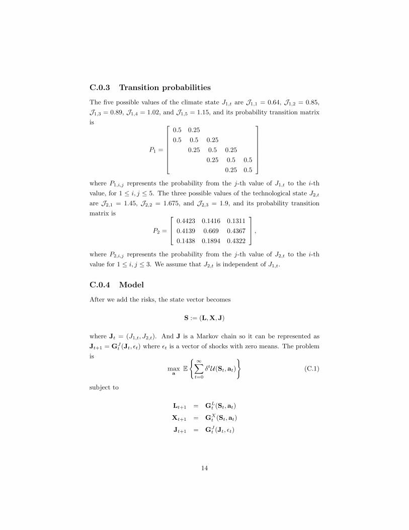
C.0.3 Transition probabilities
The five possible values of the climate state J1,t are J1,1 = 0.64, J1,2 = 0.85,
J1,3 = 0.89, J1,4 = 1.02, and J1,5 = 1.15, and its probability transition matrix
is
P1 =
2
6666664
0.5 0.25
0.5 0.5 0.25
0.25 0.5 0.25
0.25 0.5 0.5
0.25 0.5
3
7777775
where P1,i,j represents the probability from the j-th value of J1,t to the i-th
value, for 1 i, j 5. The three possible values of the technological state J2,t
are J2,1 = 1.45, J2,2 = 1.675, and J2,3 = 1.9, and its probability transition
matrix is
P2 =
2
640.4423 0.1416 0.1311
0.4139 0.669 0.4367
0.1438 0.1894 0.4322
3
75 ,
where P2,i,j represents the probability from the j-th value of J2,t to the i-th
value for 1 i, j 3. We assume that J2,t is independent of J1,t.
C.0.4 Model
After we add the risks, the state vector becomes
S := (L,X,J)
where Jt = (J1,t, J2,t). And J is a Markov chain so it can be represented as
Jt+1 = GJt (Jt, ✏t) where ✏t is a vector of shocks with zero means. The problem
is
maxa
E( 1X
t=0
�tU(St,at)
)(C.1)
subject to
Lt+1 = GLt (St,at)
Xt+1 = GXt (St,at)
Jt+1 = GJt (Jt, ✏t)
14

and at 2 Dt(St) representing the feasibility constraints, that is, inequality con-
straints and the equations other than the above transition laws. The above
transition laws are just a special case of
St+1 = Gt(St,at, ✏t)
in the notations of Section 2, so we can implement our ENLCEQ method to
solve the dynamic stochastic programming problem. Since our time of interest
is T = 100 years, in ENLCEQ we choose bT = 400 so that a larger bT will have
little change on our solution at the first 100 years.
In the step 2 of Algorithm 1 for solving the solution at time s, we replace ✏t
by its zero mean to have St+1 = Gt(St,at, 0), that is, Jt+1 = GJt (Jt, 0). But
this Jt+1 = GJt (Jt, 0) is only for simplicity in notations. In fact, since J is a
Markov chain, we replace Jt by its mean conditional on the realized value of Js
(i.e., its certainty equivalent approximation):
[J1⇡1,t,s, J2⇡2,t,s]
for all t � s, where J1 = (J1,1, ...,J1,5), J2 = (J2,1,J2,2,J2,3), ⇡1,t,s and ⇡2,t,s
are two column vectors representing probability distributions of J1,t and J2,t
conditional on the realized values of J1,s and J2,s respectively. If the realized
values of J1,s and J2,s are J1,i and J2,j respectively, then we have ⇡1,t,s =
P t�s1 ⇡1,s,s and ⇡2,t,s = P t�s
2 ⇡2,s,s, where ⇡1,s,s is a length-5 column vector with
1 at the ith element and 0 everywhere else, and ⇡2,s,s is a length-3 column vector
with 1 at the jth element and 0 everywhere else.
C.1 Model Equations, Variables and Parame-
ters
C.1.1 Equations
Land Use
L =X
i=A,P,C,N,R
Lit (C.2)
LNt+1 = LN
t ��N,At ��N,R
t +�C,Nt (C.3)
15
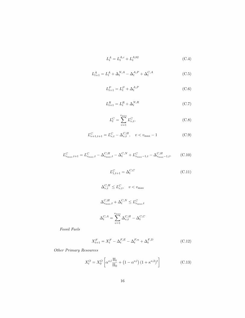
LAt = LA,c
t + LA,b2t (C.4)
LAt+1 = LA
t +�N,At ��A,P
t +�C,At (C.5)
LPt+1 = LP
t +�A,Pt (C.6)
LRt+1 = LR
t +�N,Rt (C.7)
LCt =
vmaxX
v=1
LCv,t, (C.8)
LCv+1,t+1 = LC
v,t ��C,Hv,t , v < vmax � 1 (C.9)
LCvmax,t+1 = LC
vmax,t ��C,Hvmax,t ��C,N
t + LCvmax�1,t ��C,H
vmax�1,t, (C.10)
LC1,t+1 = �C,C
t (C.11)
�C,Hv,t LC
v,t, v < vmax
�C,Hvmax,t +�C,N
t LCvmax,t
�C,At =
vmaxX
v=1
�C,Hv,t ��C,C
t
Fossil Fuels
XFt+1 = XF
t ��F,Et ��F,n
t +�F,Dt (C.12)
Other Primary Resources
XOt = XO
0
↵o,l ⇧t
⇧0+�1� ↵o,l
�(1 + o,2)t
�(C.13)
16

Intermediate Products
xpt = ✓pt�
F,Et (C.14)
xnt = ✓n�F,n
t (C.15)
xnt = xn,c
t + xn,b2t (C.16)
xct = ✓ct
⇣↵n⇣LA,ct
⌘⇢n
+ (1� ↵n) (xn,ct )
⇢n
⌘ 1⇢n
(C.17)
xc,b2t = ✓c,b2t
⇣↵n⇣LA,b2t
⌘⇢n
+ (1� ↵n)⇣xn,b2t
⌘⇢n⌘ 1
⇢n(C.18)
xb1t = ✓b1xc,b
t (C.19)
xb2t = ✓b2
✓�↵b2�✓b2,K
t (K)⇢b2 +�1� ↵b2
� ⇣xc,b2t
⌘⇢b2◆ 1
⇢b2
(C.20)
xlt = ✓P
⇣↵l�LPt
�⇢l+�1� ↵l
� ⇣xc,lt
⌘⇢l⌘ 1
⇢l(C.21)
xwt =
vmaxX
v=1
✓wv,t�C,Hv,t (C.22)
Final Goods and Services
Y ft = ✓ft
�xc � xc,b � xc,l
�(C.23)
Y et = ✓et
⇣↵e�xb1t
�⇢e+ (1� ↵e)
�xpt + xb2
t
�⇢e⌘ 1
⇢e(C.24)
Y lt = ✓ltx
lt, (C.25)
Y wt = ✓yw
t xwt (C.26)
17

Y rt = ✓r
2
4X
i=A,P,C
↵i,r�Lit
�⇢r +
0
@1�X
i=A,P,C
↵i,r
1
A�LNt + ✓RLR
t
�⇢r
3
5
1⇢r
(C.27)
Y ot = ✓o,1t
2
664
XOt � 1
✓o0[co,c xc
tAt
+ co,cb xc,b2t
✓c,b2t
+ co,f Y ft
✓ft
+ co,pxpt + co,nxn
t + co,bxb1t
+co,b2xb2t + co,lxl
t + co,yl ✓l0Y
lt
✓lt
+ co,wt �C,Ht + co,ywxw
t
+co,rLRt + cp�C,C
t + CNt + CR
t + CFt + CH
t + CPt + CC,N
t ]
3
775
(C.28)
yt =⇣yft , y
lt, y
et , y
wt , y
rt , y
ot
⌘=⇣Y ft , Y l
t , Yet , Y
wt , Y r
t , Yot
⌘/⇧t (C.29)
Technology (deterministic)
At =ATA0ect
AT +A0 (ect � 1)(C.30)
✓wv,t =
8<
:0.00001 if v v
✓wv (1 + wv t) if v > v
, ✓wv = exp
✓ a �
b
(v � v)
◆(C.31)
✓it = ✓i0(1 + i)t, i = f, e, l, yw, o (C.32)
Technology (stochastic)
At =AT (J1,t, J2,t)A0ect
AT (J1,t, J2,t) +A0 (ect � 1)(C.33)
Costs
CN,A,Rt = ⇠n0
⇣�N,A
t +�N,Rt
⌘+ ⇠n1
⇣�N,A
t +�N,Rt
⌘2(C.34)
CN,Rt = ⇠R0 �
N,Rt + ⇠R1
⇣�N,R
t
⌘2(C.35)
CFt = ⇠F1
⇣�F,E
t +�F,nt
⌘2✓XF0 +�F,D
XFt +�F,D
◆(C.36)
CHt = ⇠H0
⇣�C,H
t ��C,Ct
⌘2+X
v
⇠H1LCv,t+1 + ⇠H2
(C.37)
18
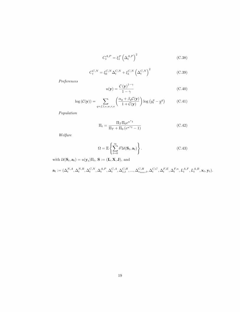
CA,Pt = ⇠P1
⇣�A,P
t
⌘2(C.38)
CC,Nt = ⇠C,N
0 �C,Nt + ⇠C,N
1
⇣�C,N
t
⌘2(C.39)
Preferences
u(y) =C (y)1��
1� �(C.40)
log (C(y)) =X
q=f,l,e,w,r,o
✓↵q + �qC(y)1 + C(y)
◆log�yqt � yq
�(C.41)
Population
⇧t =⇧T⇧0e
⇡t
⇧T +⇧0 (e⇡t � 1)
(C.42)
Welfare
⌦ = E( 1X
t=0
�tU(St,at)
). (C.43)
with U(St,at) = u(yt)⇧t, S := (L,X,J), and
at := (�N,At ,�N,R
t ,�C,Nt ,�A,P
t ,�C,At ,�C,H
1,t , ...,�C,Hvmax,t,�
C,Ct ,�F,E
t ,�F,nt , LA,F
t , LA,Bt ,xt,yt).
19

C.1.2 Tables
Table C.1: Model Exogenous Variables
Parameter Description Units
Exogenous Variables
�F,Dt Flow of Newly Discovered Fossil Fuels trillion toe
XOt Other Primary Goods trillion USD
At Crop Technology Index✓c,b2t 2G biofuels Crop Technology Index✓b2,Kt 2G Biofuels Fixed Factor Decay Index✓wv,t Logging Productivity Index
✓ft Food Processing Productivity Index✓et Energy E�ciency Index✓lt Livestock Processing Productivity Index
✓yw
t Wood Processing Productivity Index✓ot Total Factor Productivity IndexCF
t Fossil Fuel Extraction Cost share of XOt
CNt Natural Land Access Cost share of XO
t
CRt Natural Land Protection Cost share of XO
t
CHt Managed Forest Conversion Cost share of XO
t
CPt Pasture Land Conversion Cost share of XO
t
CC,Nt Natural Land Restoration Cost share of XO
t
⇧t Population billion people
20

Table C.2: Model Endogenous Variables
Parameter Description Units
LAt Agricultural Land Area GHa
LA,ct Agricultural Land Area, food crops GHa
LA,b2t Agricultural Land Area, 2G biofuels crops GHa
LPt Pasture Land Area GHa
LCt Commercial Forest Land Area GHa
LNt Unmanaged Natural Land Area GHa
LRt Protected Natural Land Area GHa
�N,At Flow of Deforested Natural Land GHa
�N,Rt Flow of Protected Natural Land GHa
�C,Nt Flow of Restored Natural Land GHa
�C,At Managed Forest Land Converted to Agriculture GHa
�C,Ct Replanted Forest Land Area GHa
�C,Hv,t Harvested Forest Land Area of Vintage v GHa
�A,Pt Agricultural Land Converted to Pasture GHa
XFt Stock of Fossil Fuels Ttoe
�F,Et Flow of Fossil Fuels Converted to Petroleum Ttoe
�F,nt Flow of Fossil Fuels Converted to Fertilizers Ttoe
xpt Petroleum Products Gtoe
xnt Fertilizers Gton
xct Food Crops Gton
xc,b2t 2G Biofuels Crops Gton
xb1t 1G Biofuels Gtoe
xb2t 2G Biofuels Gtoe
xlt Livestock Gtoe
xwt Raw Timber Gton
Y ft Services from Processed Food billion USD
Y et Energy Services billion USD
Y lt Services from Processed Livestock billion USD
Y wt Services from Processed Timber billion USD
Y rt Eco-system Services billion USD
Y ot Other Goods and Services trillion USD
21

Table C.3: Baseline Parameters
Parameter Description Units Value
Population
⇧0 Population in 2004 billion people 6.39⇧T Population in time T billion people 10.1⇡ Population Convergence Rate 0.042
Land Use
L Total Land Area billion Ha 8.56LA0 Area of Agricultural Land in 2004 billion Ha 1.53
LP0 Area of Pasture Land in 2004 billion Ha 2.73
LC0 Area of Commercial Forest Land in 2004 billion Ha 1.62
LN0 Area of Unmanaged Natural Land in 2004 billion Ha 2.47
LR0 Area of Protected Natural Land in 2004 billion Ha 0.207
⇠n0 Access Cost Function Parameter 0.6⇠n1 Access Cost Function Parameter 105⇠R0 Protection Cost Function Parameter 4.5⇠R1 Protection Cost Function Parameter 400⇠P1 Pasture Conversion Cost Function Parameter 170⇠H0 Forest Conversion Cost Function Parameter 80⇠H1 Forest Conversion Cost Function Parameter 0.004⇠C,N0 Natural Land Restoration Cost Parameter 0.8⇠C,N1 Natural Land Restoration Cost Parameter 400
Fossil Fuels
XF0 Endowment of Fossil fuels in 2004 trillion toe 0.343
�F,D Flow of Newly Discovered Fossil Fuels trillion toe 0.008⇠F1 Fuel Extraction Cost Function Parameter 2000
Other Primary Goods
XO0 Endowment of Other Primary Goods in 2004 USD ⇥ 1013 3.16
o,X Growth Rate of Physical Capital 0.0035↵o,l Share of demographic factors in growth of XO
t 0.39
Intermediate Products
✓p Petroleum Conversion Factor per toe of �F,Et 0.5
co,p Petroleum Conversion Cost share of XOt 0.0157
22

Table C.3: Baseline Parameters (continued)
Parameter Description Units Value
✓n Fertilizer Conversion Factor Tton / Ttoe 1.071co,n Fertilizer Conversion Cost share of XO
t 0.0021✓b1 1G Biofuels Conversion Rate toe/ton 0.283✓b2 2G Biofuels Conversion Rate toe/ton 0.467K 2G Biofuels Fixed Factor Index 0.005co,b1 1G Biofuels Conversion Cost share of XO
t 0.00025co,b2 2G Biofuels Conversion Cost share of XO
t 0.00033an Share of Agricultural Land in CES function 0.55⇢n CES Parameter for Agricultural Land and
Fertilizers0.123
A0 Crop Technology Index in 2004 13.89c Logistic Growth Rate of Crop Technology Index 0.025co,c Food Crop Production Cost share of XO
t 0.016✓c,b20 2G Biofuels Crop Technology Index in 2004 14.89b2 2G Biofuels Fixed Factor Decay Rate 0.05↵b2 Fixed Factor Cost Share in 2G Biofuels
Production0.6
⇢b2 CES Parameter for Fixed Factor andAgriculturalLand
-1.5
co,c 2G Biofuels Crops Production Cost share of XOt 0.022
✓P Livestock Technology Index in 2004 0.69al Share of Pasture Land in CES function 0.35⇢l CES Parameter for Pasture Land and Feed -0.33co,l Livestock Production Cost share of XO
t 0.0055 a Merchantable Timber Yield Parameter 1 5.62 b Merchantable Timber Yield Parameter 2 76.5v Minimum Age for Merchantable Timber Years 11wv Timber Yield Gains of Vintage v Share of Yield 0 0.011cp Forest Planting Cost share of XO
t 0.0001co,w Forest Harvesting Cost share of XO
t 0.0021
Final Goods and Services
✓f0 Food Processing Technology Index in 2004 1.5f Food Processing Technology Index Growth
Rate0.0225
co,f Food Processing Cost share of XOt 0.015
✓l0 Livestock Processing Technology Index in 2004 1.7l Livestock Processing Technology Growth Rate 0.0025co,yl Livestock Processing Cost share of XO
t 0.0068
23
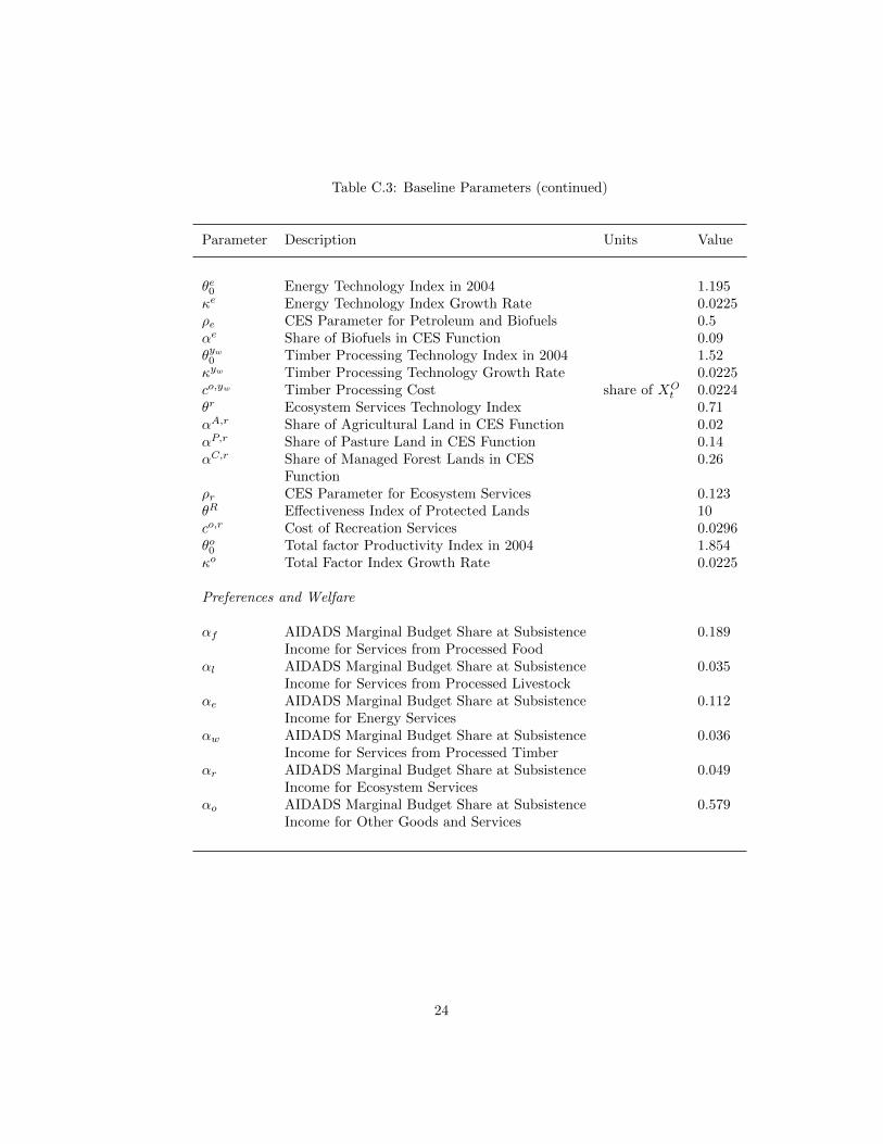
Table C.3: Baseline Parameters (continued)
Parameter Description Units Value
✓e0 Energy Technology Index in 2004 1.195e Energy Technology Index Growth Rate 0.0225⇢e CES Parameter for Petroleum and Biofuels 0.5↵e Share of Biofuels in CES Function 0.09✓yw0 Timber Processing Technology Index in 2004 1.52yw Timber Processing Technology Growth Rate 0.0225co,yw Timber Processing Cost share of XO
t 0.0224✓r Ecosystem Services Technology Index 0.71↵A,r Share of Agricultural Land in CES Function 0.02↵P,r Share of Pasture Land in CES Function 0.14↵C,r Share of Managed Forest Lands in CES
Function0.26
⇢r CES Parameter for Ecosystem Services 0.123✓R E↵ectiveness Index of Protected Lands 10co,r Cost of Recreation Services 0.0296✓o0 Total factor Productivity Index in 2004 1.854o Total Factor Index Growth Rate 0.0225
Preferences and Welfare
↵f AIDADS Marginal Budget Share at SubsistenceIncome for Services from Processed Food
0.189
↵l AIDADS Marginal Budget Share at SubsistenceIncome for Services from Processed Livestock
0.035
↵e AIDADS Marginal Budget Share at SubsistenceIncome for Energy Services
0.112
↵w AIDADS Marginal Budget Share at SubsistenceIncome for Services from Processed Timber
0.036
↵r AIDADS Marginal Budget Share at SubsistenceIncome for Ecosystem Services
0.049
↵o AIDADS Marginal Budget Share at SubsistenceIncome for Other Goods and Services
0.579
24
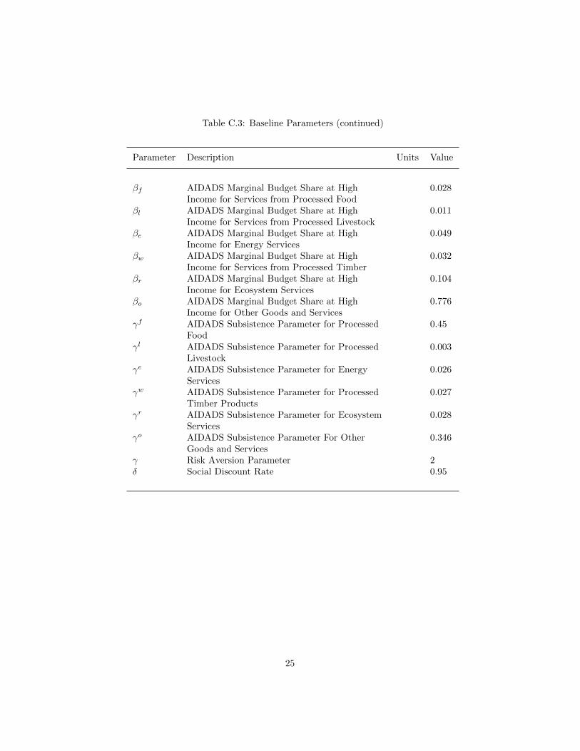
Table C.3: Baseline Parameters (continued)
Parameter Description Units Value
�f AIDADS Marginal Budget Share at HighIncome for Services from Processed Food
0.028
�l AIDADS Marginal Budget Share at HighIncome for Services from Processed Livestock
0.011
�e AIDADS Marginal Budget Share at HighIncome for Energy Services
0.049
�w AIDADS Marginal Budget Share at HighIncome for Services from Processed Timber
0.032
�r AIDADS Marginal Budget Share at HighIncome for Ecosystem Services
0.104
�o AIDADS Marginal Budget Share at HighIncome for Other Goods and Services
0.776
�f AIDADS Subsistence Parameter for ProcessedFood
0.45
�l AIDADS Subsistence Parameter for ProcessedLivestock
0.003
�e AIDADS Subsistence Parameter for EnergyServices
0.026
�w AIDADS Subsistence Parameter for ProcessedTimber Products
0.027
�r AIDADS Subsistence Parameter for EcosystemServices
0.028
�o AIDADS Subsistence Parameter For OtherGoods and Services
0.346
� Risk Aversion Parameter 2� Social Discount Rate 0.95
25
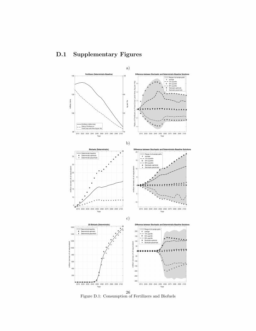
D.1 Supplementary Figures
a)
2010 2020 2030 2040 2050 2060 2070 2080 2090 2100
Year
80
100
120
140
mill
ion
ton
s
Fertilizers (Deterministic-Baseline)
40
60
80
100
kg p
er
Ha
Fertilizers (million tons)
Ratio of Fertilizers to
Food Crop Land Area (kg per Ha)
Difference between Stochastic and Deterministic-Baseline Solutions
2010 2020 2030 2040 2050 2060 2070 2080 2090 2100
Year
-4
-2
0
2
4
6
Ratio o
f F
ert
ilize
rs t
o F
oo
d C
rop
La
nd
Are
a (
kg
per
Ha)
Range of all sample paths
average
10% quantile
50% quantile
90% quantile
Stochastic-optimistic
Stochastic-pessimistic
b)
2010 2020 2030 2040 2050 2060 2070 2080 2090 2100
Year
5
10
15
20
25
30
35
mill
ion tonnes o
f oil
equiv
ale
nt
Biofuels (Deterministic)
Deterministic-baseline
Deterministic-optimistic
Deterministic-pessimistic
Difference between Stochastic and Deterministic-Baseline Solutions
2010 2020 2030 2040 2050 2060 2070 2080 2090 2100
Year
-10
-5
0
5
10
15
20
mill
ion tonnes o
f oil
equiv
ale
nt
Range of all sample paths
average
10% quantile
50% quantile
90% quantile
Stochastic-optimistic
Stochastic-pessimistic
c)
2010 2020 2030 2040 2050 2060 2070 2080 2090 2100
Year
200
400
600
800
1000
1200
1400
1600
millio
n t
on
ne
s o
f o
il e
qu
iva
len
t
2G Biofuels (Deterministic)
Deterministic-baseline
Deterministic-optimistic
Deterministic-pessimistic
Difference between Stochastic and Deterministic-Baseline Solutions
2010 2020 2030 2040 2050 2060 2070 2080 2090 2100
Year
-300
-250
-200
-150
-100
-50
0
50
100
150
200
millio
n t
on
ne
s o
f o
il e
qu
iva
len
t
Range of all sample paths
average
10% quantile
50% quantile
90% quantile
Stochastic-optimistic
Stochastic-pessimistic
Figure D.1: Consumption of Fertilizers and Biofuels26

D.1 Error Checking
For a simulated path i, at the current time s, we use the step 2 of Algorithm
1 to find the optimal decision ais at its current state Sis. Its next state in the
original stochastic model (1) is Gs(Sis,a
is, ✏s) which is random and dependent
on ✏s 2 ⇥, where ⇥ represents the set of all possible vectoral values of ✏s. The
associated Euler equation for the stochastic model is
�s = �Es
✓rSs+1Gs+1(Gs(S
is,a
is, ✏s),as+1, ✏s+1)�s+1
+rSs+1Hs+1(Gs(Sis,a
is, ✏s),as+1)µs+1
◆(D.1)
where rSs+1 is the gradient operator over Ss+1, �t�t is the multiplier (a column
vector) of the constraint St+1 = Gt(St,at, ✏t) and �tµt is the multiplier (a col-
umn vector) of the feasibility constraints at 2 Dt(St) which are represented by
Ht(St,at) � 0 here.8 In the literature, the multipliers are often substituted by
marginal utilities or some other expressions derived from Karush–Kuhn–Tucker
conditions, but we keep them in the equation as such substitutions are often
complicated (e.g., in our examples) and we can directly get the multipliers from
numerical optimization solvers. The multipliers and as+1 can be approximated
by the solutions in the deterministic model (2) at their corresponding states.
For example, we compute Si,js+1 = Gs(Si
s,ais, ✏
js) for every possible ✏js 2 ⇥ and
then use the step 2 of Algorithm 1 to find the optimal decision ai,js+1 at its asso-
ciate state Si,js+1 at time s+ 1 and their corresponding multipliers, and then we
can compute the expectation in equation (D.1) as the conditional probability
distribution of ✏s is given. When ✏s is a continuous random variable vector, we
can use its quadrature nodes ✏js and then implement quadrature rules to esti-
mate the expectation in equation (D.1). Thus, for the simulated path i, we can
compute the normalized Euler error at time s:
E is =
�����Es
✓rSs+1Gs+1(Gs(S
is,a
is, ✏s),as+1, ✏s+1)
�s+1
�s
+rSs+1Hs+1(Gs(Sis,a
is, ✏s),as+1, ✏s+1)
µs+1
�s
◆� 1
����
8An equality constraint f(x) = 0 can be written as a combination of f(x) � 0 and �f(x) �0.
27
where 1 is a vector of ones, �s+1
�sand µs+1
�sare elementwise divisions, and k·k is
a norm operator. Note that the normalized Euler error is unit free.
For our stochastic FABLE model, we find that the approximate L1 error of
the first 100 years solutions among 1,000 simulated paths, defined as
max1s100
1
1000
1000X
i=1
E is
!,
is only 8.6⇥ 10�4, and the corresponding approximate L1 error, defined as
max1s100
✓max
1i1000E is
◆,
is only 0.02. Thus, we see that ENLCEQ solves our stochastic model within an
acceptable accuracy.
D.2 An Illustrative Example
Below we use a simple optimal growth model to illustrate ENLCEQ. We assume
the total factor of productivity, At, is a Markov chain. It has three possible
values: A1 = 0.9, A2 = 1.0, and A3 = 1.1. Its transition probability matrix is
P =
2
640.8 0.2
0.2 0.6 0.2
0.2 0.8
3
75 .
We use At+1 = GA(At, ✏t) to represent the transition law of At, where ✏t is
a random variable with zero mean. We solve the following optimal growth
problem:
max E( 1X
t=0
�tu(ct)
)(D.2)
s.t. kt+1 = (1� �)kt +Atk↵t � ct,
k0 = 1, A0 = 1,
where ct is consumption at time t, � = 0.96 is the discount factor, kt is capital,
� = 0.1 is the depreciation rate, ↵ = 0.3, and u(c) = �c�1 is the utility
function. Assume that we are interested in the solutions in the first 20 periods
(i.e., T = 20). Here in the notations of Section 2, S := (k,A) is the vector of
28

state variables, a := c is the decision variable, and the transition laws are
kt+1 = Gk(kt, at) = (1� �)kt +Atk↵t � ct
At+1 = GA(At, ✏t)
which can be written as St+1 = G(St,at, ✏t).
In ENLCEQ, we choose bT = 200 which has been large enough for the so-
lutions in the periods of our interest (i.e., the first 20 periods). If we are in-
terested in solutions at more periods, then we can also increase bT . In the step
2 of Algorithm 1 for solving problems at time s, we let St+1 = G(St,at, 0),
that is, At+1 = GA(At, 0), which in fact means that we replace At by its
mean conditional on the realized values of As: A⇡t,s, for all t � s, where
A = (A1,A2,A3) and ⇡t,s is a column vector representing the probability dis-
tribution conditional on the realized values of As. If the realized values of As is
Ai, we have ⇡t,s = P t�s⇡s,s, where ⇡s,s is a length-3 column vector with 1 at
the ith element and 0 everywhere else.
In the GAMS code attached in the end of the appendix, we compute 1,000
simulated paths of the first 20 periods which are the periods of interest. It
took 15 minutes on a laptop, much slower than NLCEQ, as ENLCEQ solves
20,000 optimization methods while NLCEQ just needs to solve a few (e.g., 33
optimization problems to obtain a degree-10 Chebyshev polynomial of k for
each of three values of A to approximate the optimal policy functions) for this
simple illustrative case. But as discussed in Section 2, ENLCEQ can solve many
problems that NLCEQ cannot or is less e�cient or less accurate.
Each simulation path i from ENLCEQ contains a pair of (kENLCEQt,i , AENLCEQ
t,i , cENLCEQt,i )
at each time t, where AENLCEQt,i is simulated exogenously. We also apply value
function iteration to solve this simple problem and then get the optimal policy
function for consumption: CV FI(k,A), which is approximated by a degree-20
Chebyshev polynomial of k on [0.5, 5] for each possible value of A. We then
compare cENLCEQt,i and CV FI(kENLCEQ
t,i , AENLCEQt,i ) for all 1 i 1000 and
t 20. We find that the approximate L1 relative error is 3.7 ⇥ 10�3 and the
approximate L1 relative error is 5.5 ⇥ 10�3. This tells us that ENLCEQ can
achieve 2 to 3 digit accuracy, which is consistent with the accuracy of NLCEQ
in Cai et al. (2017).
29

References
Alexandratos, N. 2011. Critical Evaluation of Selected Projections. Pages 465–
508 of: Conforti, P. (ed), Economic Analysis of Land Use in Global Climate
Change Policy. Food and Agriculture Organization of the United Nations,
Rome.
Alston, Julian M., & Pardey, Philip G. 2014 (Jan.). Agricultural R&D, Food
Prices, Poverty and Malnutrition Redux. Sta↵ Paper P14-01. University of
Minnesota, Department of Applied Economics.
Barbier, Edward B, Burgess, Joanne C, Bishop, Joshua, & Aylward, Bruce.
1994. The Economics of the Tropical Timber Trade. Earthscan, London
(UK).
Bentsen, M, Bethke, I, Debernard, JB, Iversen, T, Kirkevag, A, Seland, Ø,
Drange, H, Roelandt, C, Seierstad, IA, Hoose, C, et al. . 2012. The Norwegian
Earth System Model, NorESM1-M-Part 1: Description and Basic Evaluation.
Geoscientific Model Development Discussions, 5, 2843–2931.
Bondeau, Alberte, Smith, Pascalle C, Zaehle, Sonke, Schapho↵, Sibyll, Lucht,
Wolfgang, Cramer, Wolfgang, Gerten, Dieter, LOTZE-CAMPEN, HER-
MANN, Muller, Christoph, Reichstein, Markus, et al. . 2007. Modelling the
Role of Agriculture for the 20th Century Global Terrestrial Carbon Balance.
Global Change Biology, 13(3), 679–706.
Cai, Y., Judd, K.L., & Steinbuks, J. 2017. A Nonlinear Certainty Equivalent
Approximation Method for Dynamic Stochastic Problems. Quantitative Eco-
nomics, 8(1), 117–147.
Cassman, K.G., Grassini, P., & van Wart, J. 2010. Crop Yield Potential, Yield
Trends, and Global Food Security in a Changing Climate. Pages 37–51 of:
Hillel, D., & Rosenzweig, C. (eds), Handbook of Climate Change and Agroe-
cosystems. Imperial College Press.
Collins, W.J., Bellouin, N., Doutriaux-Boucher, M., Gedney, N., Hinton, T.,
Jones, C.D., Liddicoat, S., Martin, G., et al. . 2008. Evaluation of the
HadGEM2 Model. Hadley Center Tech. Note, 74.
Deryng, Delphine, Sacks, WJ, Barford, CC, & Ramankutty, N. 2011. Simulating
the E↵ects of Climate and Agricultural Management Practices on Global Crop
Yield. Global Biogeochemical Cycles, 25(2).
30

Deryng, Delphine, Elliott, Joshua, Folberth, Christian, Muller, Christoph,
Pugh, Thomas AM, Boote, Kenneth J, Conway, Declan, Ruane, Alex C,
Gerten, Dieter, Jones, James W, et al. . 2016. Regional Disparities in the
Beneficial E↵ects of Rising CO2 Concentrations on Crop Water Productivity.
Nature Climate Change, 6(8), 786.
Dufresne, J-L, Foujols, M-A, Denvil, S, Caubel, A, Marti, O, Aumont, O, Balka-
nski, Y, Bekki, Slimane, Bellenger, H, Benshila, R, et al. . 2012. Climate
Change Projections using the IPSL-CM5 Earth System Model: from CMIP3
to CMIP5. Climate Dynamics, 1–43.
Dunne, John P, John, Jasmin G, Shevliakova, Elena, Stou↵er, Ronald J, Krast-
ing, John P, Malyshev, Sergey L, Milly, PCD, Sentman, Lori T, Adcroft,
Alistair J, Cooke, William, et al. . 2013. GFDL’s ESM2 Global Coupled Cli-
mate?Carbon Earth System Models. Part II: Carbon System Formulation and
Baseline Simulation Characteristics. Journal of Climate, 26(7), 2247–2267.
Elliott, Joshua, Deryng, Delphine, Muller, Christoph, Frieler, Katja, Konzmann,
Markus, Gerten, Dieter, Glotter, Michael, Florke, Martina, Wada, Yoshihide,
Best, Neil, et al. . 2014a. Constraints and Potentials of Future Irrigation
Water Availability on Agricultural Production Under Climate Change. Pro-
ceedings of the National Academy of Sciences, 111(9), 3239–3244.
Elliott, Joshua, Kelly, David, Chryssanthacopoulos, James, Glotter, Michael,
Jhunjhnuwala, Kanika, Best, Neil, Wilde, Michael, & Foster, Ian. 2014b.
The Parallel System for Integrating Impact Models and Sectors (pSIMS).
Environmental Modelling & Software.
Fischer, T.R., Byerlee, D., & Edmeades, G.O. 2011. Can Technology Deliver on
the Yield Challenge to 2050? Pages 389–462 of: Conforti, P. (ed), Economic
Analysis of Land Use in Global Climate Change Policy. Food and Agriculture
Organization of the United Nations, Rome.
Golub, A., Hertel, T.W., & Sohngen, B. 2009. Land Use Modeling in
Recursively-Dynamic GTAP Framework. Pages 235–278 of: Hertel, T.W.,
Rose, S., & Tol, R.S.J. (eds), Economic Analysis of Land Use in Global Cli-
mate Change Policy. Routledge.
Grassini, Patricio, Eskridge, Kent M, & Cassman, Kenneth G. 2013. Distin-
guishing between Yield Advances and Yield Plateaus in Historical Crop Pro-
duction Trends. Nature Communications, 4.
31
Hertel, T.W., Steinbuks, J., & Tyner, W. 2016. What is the Social Value of
Second Generation Biofuels? Applied Economic Perspectives and Policy,
38(4), 599–617.
IPCC. 2014. Climate Change 2014: Impacts, Adaptation and Vulnerability:
Contribution of Working Group II to the Fifth Assessment Report of the In-
tergovernmental Panel on Climate Change. Cambridge University Press.
Jagermeyr, Jonas, Gerten, D, Schapho↵, S, Heinke, J, Lucht, W, & Rockstrom,
Johan. 2016. Integrated Crop Water Management Might Sustainably Halve
the Global Food Gap. Environmental Research Letters, 11(2), 025002.
Jones, James W, Hoogenboom, G, Porter, CH, Boote, KJ, Batchelor, WD,
Hunt, LA, Wilkens, PW, Singh, U, Gijsman, AJ, & Ritchie, JT. 2003. The
DSSAT Cropping System Model. European Journal of Agronomy, 18(3), 235–
265.
Licker, Rachel, Johnston, Matt, Foley, Jonathan A, Barford, Carol, Kucharik,
Christopher J, Monfreda, Chad, & Ramankutty, Navin. 2010. Mind the Gap:
How do Climate and Agricultural Management Explain the ’Yield Gap’ of
Croplands around the World? Global Ecology and Biogeography, 19(6), 769–
782.
Liu, Junguo, Williams, Jimmy R, Zehnder, Alexander JB, & Yang, Hong. 2007.
GEPIC–Modelling Wheat Yield and Crop Water Productivity with High Res-
olution on a Global Scale. Agricultural Systems, 94(2), 478–493.
Lobell, David B, Cassman, Kenneth G, & Field, Christopher B. 2009. Crop
Yield Gaps: their Importance, Magnitudes, and Causes. Annual Review of
Environment and Resources, 34(1), 179.
Long, SP. 1991. Modification of the Response of Photosynthetic Productivity to
Rising Temperature by Atmospheric CO2 Concentrations: Has its Importance
been Underestimated? Plant, Cell & Environment, 14(8), 729–739.
Long, Stephen P, Ainsworth, Elizabeth A, Leakey, Andrew DB, Nosberger,
Josef, & Ort, Donald R. 2006. Food for Thought: Lower-Than-Expected
Crop Yield Stimulation with Rising CO2 Concentrations. Science, 312(5782),
1918–1921.
32
Moss, Richard H, Babiker, Mustafa, Brinkman, Sander, Calvo, Eduardo, Carter,
Tim, Edmonds, James A, Elgizouli, Ismail, Emori, Seita, Lin, Erda, Hibbard,
Kathy, et al. . 2008. Towards New Scenarios for Analysis of Emissions, Cli-
mate Change, Impacts, and Response Strategies. Tech. rept. PNNL-SA-63186.
Pacific Northwest National Laboratory (PNNL), Richland, WA (US).
Nordhaus, William D, & Boyer, Joseph. 2000. Warming the World: Economic
Models of Global Warming. MIT press.
Rimmer, M.T., & Powell, A.A. 1996. An Implicitly Additive Demand System.
Applied Economics, 28(12), 1613–1622.
Rosenzweig, C., Elliott, J., Deryng, D., Ruane, A.C., Arneth, A., Bootef, K.J.,
Folberth, C., Glotter, M., Khabarov, N., Muller, C., Neumann, K., Piontek,
F., Pugh, T., Schmid, E., Stehfest, E., & Jones, J.W. 2014. Assessing Agricul-
tural Risks of Climate Change in the 21st Century in a Global Gridded Crop
Model Intercomparison. Proceedings of the National Academy of Sciences,
111(9), 3268–3273.
Steinbuks, J., & Hertel, T.W. 2016. Confronting the Food-Energy-Environment
Trilemma: Global Land Use in the Long Run. Environmental and Resource
Economics, 63(3), 545–570.
Watanabe, S, Hajima, T, Sudo, K, Nagashima, T, Takemura, T, Okajima, H,
Nozawa, T, Kawase, H, Abe, M, Yokohata, T, et al. . 2011. MIROC-ESM
2010: Model Description and Basic Results of CMIP5-20c3m Experiments.
Geoscientific Model Development, 4, 845–872.
33