E. Boniolo: Critical Behaviour of a Marriage...
125
Corso di Laurea in Fisica Critical Behaviour of a Marriage Problem Relatore: Prof. Sergio Caracciolo Correlatore: Dott. Andrea Sportiello Tesi di Laurea di: Elena Boniolo Matricola: 506125 Codice PACS: 02.50.-r Anno Accademico: 2011-2012
Transcript of E. Boniolo: Critical Behaviour of a Marriage...

Corso di Laurea in Fisica
Critical Behaviour ofa Marriage Problem
Relatore: Prof. Sergio Caracciolo
Correlatore: Dott. Andrea Sportiello
Tesi di Laurea di:Elena BonioloMatricola: 506125
Codice PACS: 02.50.-r
Anno Accademico: 2011-2012

02.50.-r Probability theory, stochastic processes, and statistics

Contents
Introduction 1
1 Statistical mechanics and combinatorial optimisation 5
1.1 Statistical mechanics and critical phenomena . . . . . . . . . . . 5
1.1.1 Classical equilibrium statistical mechanics . . . . . . . . 5
1.1.2 Phase transitions . . . . . . . . . . . . . . . . . . . . . . 6
1.2 Combinatorial optimisation . . . . . . . . . . . . . . . . . . . . 9
1.2.1 Classification of optimisation problems . . . . . . . . . . 10
1.2.2 Some examples of classical problems . . . . . . . . . . . 11
1.2.3 The assignment problem . . . . . . . . . . . . . . . . . . 12
1.2.4 Combinatorial optimisation and statistical mechanics at
zero T . . . . . . . . . . . . . . . . . . . . . . . . . . . . 13
2 The Grid-Poisson Marriage 15
2.1 Marriage problems . . . . . . . . . . . . . . . . . . . . . . . . . 15
2.2 Stochastic processes . . . . . . . . . . . . . . . . . . . . . . . . . 16
2.2.1 Random variables . . . . . . . . . . . . . . . . . . . . . . 16
2.2.2 Random processes . . . . . . . . . . . . . . . . . . . . . 17
2.2.3 Point processes . . . . . . . . . . . . . . . . . . . . . . . 22
2.3 The model . . . . . . . . . . . . . . . . . . . . . . . . . . . . . . 23
3 The marriage problem in one dimension 27
3.1 Exact solution for the correlation function at density one . . . . 27
3.1.1 Definitions . . . . . . . . . . . . . . . . . . . . . . . . . . 27
3.1.2 Open boundary conditions . . . . . . . . . . . . . . . . . 30
3.1.3 Periodic boundary conditions . . . . . . . . . . . . . . . 35
3.2 Numerical simulations . . . . . . . . . . . . . . . . . . . . . . . 37
3.2.1 Choice of the weight function . . . . . . . . . . . . . . . 37
3.2.2 Numerical results at the critical point . . . . . . . . . . . 39
3.2.3 Near the critical point . . . . . . . . . . . . . . . . . . . 39
i

ii CONTENTS
4 Finite-Size Scaling in two dimensions 47
4.1 Theory of finite-size scaling . . . . . . . . . . . . . . . . . . . . 48
4.1.1 Thermodynamic limit . . . . . . . . . . . . . . . . . . . . 48
4.1.2 Scaling hypothesis . . . . . . . . . . . . . . . . . . . . . 49
4.1.3 Asymptotic form of FSS . . . . . . . . . . . . . . . . . . 50
4.1.4 Extrapolating to infinite volume . . . . . . . . . . . . . . 51
4.2 Numerical simulations . . . . . . . . . . . . . . . . . . . . . . . 52
4.2.1 Definitions . . . . . . . . . . . . . . . . . . . . . . . . . . 52
4.2.2 Qualitative behaviour of the correlation function . . . . . 54
4.2.3 Curve-fitting ansatz . . . . . . . . . . . . . . . . . . . . . 55
4.2.4 Scaling ansatz at the critical point . . . . . . . . . . . . 58
4.2.5 Determination of the parameter α . . . . . . . . . . . . . 58
4.2.6 Behaviour near the critical point: definition and study
of the correlation length . . . . . . . . . . . . . . . . . . 65
5 Probability density of the distance between matched pairs 75
5.1 Numerical results in two dimensions . . . . . . . . . . . . . . . . 76
5.1.1 At the critical point . . . . . . . . . . . . . . . . . . . . 76
5.1.2 Near the critical point . . . . . . . . . . . . . . . . . . . 87
5.2 Numerical results in one dimension . . . . . . . . . . . . . . . . 91
5.2.1 At the critical point . . . . . . . . . . . . . . . . . . . . 91
5.2.2 Near the critical point . . . . . . . . . . . . . . . . . . . 94
Conclusions and future developments 99
A Technical tools 101
A.1 Hardware . . . . . . . . . . . . . . . . . . . . . . . . . . . . . . 101
A.2 Software . . . . . . . . . . . . . . . . . . . . . . . . . . . . . . . 103
B Basic concepts of graph theory 105
B.1 Graphs and subgraphs . . . . . . . . . . . . . . . . . . . . . . . 105
B.2 Paths and cycles . . . . . . . . . . . . . . . . . . . . . . . . . . 107
C Distribution functions of random variables 109
C.1 Distribution functions . . . . . . . . . . . . . . . . . . . . . . . 109
C.2 Mean, variance and covariance . . . . . . . . . . . . . . . . . . . 110
C.3 Some special distributions . . . . . . . . . . . . . . . . . . . . . 111
Riassunto in italiano 113
Bibliography 119
Introduction
Over the last decades, it has been recognised that combinatorial optimisation
is connected with statistical mechanics in a natural way: if we identify the
instances of the optimisation problem with the configurations of the model of
statistical mechanics and the cost function with the energy, finding a solution
to a problem of minimisation corresponds to finding the ground state of the
thermodynamic system in the limit of zero temperature.
This analogy allows us to adapt the ideas and tools of statistical mechan-
ics, such as the universality of the critical exponents or the techniques of the
Renormalisation Group, to discuss optimisation problems and develop new
algorithms. Conversely, it is possible to study optimisation problem as test-
ing ground to devise and experiment techniques useful in the study of complex
physical models, such as disordered systems (spin glasses or polymer networks,
for instance, but also, in different areas, collective social behaviour or financial
markets).
In this thesis, we will consider a problem known as the “Grid-Poisson Mar-
riage”. This is defined as the optimal matching between N lattice points and
M random points in the continuum, taken with Poisson distribution. As we
will see, it is a typical assignment problem, where the weight function is given
by the sum of the Euclidean distances between the couples of points. In this
case, the problem is trivial at very high or very low densities ρ = M/N , while
the system becomes critical near ρ = 1, where there is the symmetry in the
exchange of N with M . Owing also to the underlying geometrical structure,
this is a critical phenomenon in all respects, as at ρ = 1, the searching pro-
cess of an “ideal partner” extends to all length scales and the energy density
diverges.
The importance of this model lies in its showing a non-trivial critical beha-
viour, and still being simpler to study than analogous problems. Indeed, in
this case we can make use of a very powerful weapon, the Hungarian algorithm,
1

2 INTRODUCTION
which provides us with a solution for the assignment problem in polynomial
time (O(N3)), so allowing us to perform numerical simulations at appreciable
sizes in relatively short times.
As a final remark, we want to observe that the system is not invariant under
translation, and in this sense the GPM can be used as a simple model in the
study of physical disordered systems, which are in general very difficult to deal
with.
This problem, and related models such as the Poisson-Poisson matching,
have been studied in the past and there are already some important results
(see, for instance, [20], [19], or [21]). In particular, Elia Zarinelli has discussed
this subject in his Master’s thesis [1], and the present work can be considered
as a development of his own.
Structure of the thesis
In this thesis, we study some properties of the GPM from a theoretical point of
view, and we compare them with data from numerical simulations on lattices
of different sizes and with different densities of Poisson points.
Chapter 1
We recall some basic concepts of statistical mechanics and combinatorial op-
timisation and formalise the link between these two areas of study.
Chapter 2
We give some definitions and properties of random processes, which will be
useful in the following, and we define the model under investigation.
Chapter 3
We use the properties of stochastic processes, in particular Wiener processes
and Brownian bridges, to find the exact solution for the correlation function
in one dimension at density ρ = 1.
We show that, if we consider as a weight function to minimise the sum of the
squares of the distances, the analytic solution found is in very good agreement
with the results from numerical simulations.
We also show the numerical curves at ρ 6= 1 and give a brief qualitative
description of them.

INTRODUCTION 3
Chapter 4
We state the fundamental ideas of Finite-Size Scaling of thermodynamic sys-
tems, and apply this technique to the 2-dimensonal GPM. In particular, by
means of simulations at the critical point ρ = 1, we give a numerical estimate
of the scaling of the wall-to-wall correlation function.
We show numerically the shape of the correlation function near the critical
point, give two possible definitions of correlation length and examine their
behaviour.
Chapter 5
We study the probability distribution of the edge lengths from simulations at
different sizes and densities.
In addition, we examine the mean of these lengths as a function of the size
and we verify the results presented in literature on the subject.

4 INTRODUCTION

1Statistical mechanics andcombinatorial optimisation
1.1 Statistical mechanics and critical phenom-
ena
In this section, we will introduce some basic concepts of statistical mechanics
and give a brief account of the phenomenon of phase transitions, with partic-
ular stress on the subjects of universality classes and critical exponents.
1.1.1 Classical equilibrium statistical mechanics
The main aim of statistical mechanics is to predict the relations between the
observable macroscopic properties of a mechanical system, given only a know-
ledge of the microscopic forces between the large number of particles composing
it (as an example, the molecules of a gas or the spins of a magnet).
The normal approach of Hamiltonian mechanics in this context is unreason-
able, due to the large number of degrees of freedom, and it becomes necessary
to make use of the tools of probability theory.
Let us denote by C a generic state of the system (for example, in a ferro-
magnetic substance, a state is specified once the orientation of each magnetic
dipole is known). Assume that the total number N of the spins is sufficiently
large and that the system is at thermal equilibrium. Within these assump-
tions, the probability that a given configuration C of the system is realised, is
5

6 CHAPTER 1. STATISTICAL MECHANICS AND. . .
given by the Boltzmann law
P [C] =e−βE(C)
Z, (1.1)
where E(C) is the energy of the configuration C, and β = 1/kBT (T being the
absolute temperature).
The expectation value of any physical observable O is then expressed by the
statistical average on all configurations, with weights given by the Boltzmann
law
〈O〉 =
∑C O(C)e−βE(C)
Z, (1.2)
where the quantity Z in the denominator is a normalisation factor defined by
Z(N, β) =∑C
e−βE(C). (1.3)
Z is called the partition function of the system, while the factor e−βE(C) that
gives the weight of each configuration is the Gibbs factor.
The thermodynamic quantities typical of the system at equilibrium can then
be written in terms of Z. For example, for the free energy F and the internal
energy U we have
F = − 1
βlogZ (1.4)
U = −T 2 ∂
∂T
F
T(1.5)
1.1.2 Phase transitions
When we consider systems with a macroscopic number of degrees of freedom
(N →∞), a phenomenon can occur which has no counterpart in both classical
and quantum mechanics of finite degrees of freedom: systems ruled by the same
Hamiltonian, can coexist in different phases, or undergo sudden transitions
between phases as the temperature changes. This phenomenon is known as
phase transition.
Two typical examples are the transition water-vapour at 100 and the mag-
netisation of a metallic (for instance iron) bar in the presence of an external
magnetic field ~B. If we examine the latter, we see that the magnetisation is

1.1. STATISTICAL MECHANICS AND CRITICAL PHENOMENA 7
discontinuous at zero external field, as we are in the presence of a residual
finite magnetisation M0, and it is possible to have at the same time different
regions of the sample in different magnetisation states. Moreover, if we study
the trend of the magnetisation along this discontinuity as a function of the
temperature, we see that it decreases as the temperature increases, until it
reaches the so called critical temperature Tc of the material.
Both the non-analyticity of the thermodynamic quantities and the coexist-
ence of different phases are particularly surprising. They can be understood
if we suppose the system has more than one possible local equilibrium state
(minimum of the free energy) and can go from a minimum to another only
by sudden global changes. The points in the space of parameters where the
transition occur are called critical points and it is customary to use, instead
of the parameter T (which for historical reasons is treated as a temperature,
but can be any parameter of the system), the adimensional parameter called
reduced temperature
t =T − TcTc
. (1.6)
Very often, the discontinuities of the physical observables near the critical
point show a power law in their dominant part, with possibly non-integer
exponent. These exponents are called critical exponents and have an important
role in the classification of the different systems that show phase transitions.
For example, the anomalous behaviour of the magnetisation is parametrised
by the critical exponent β:
M(B = 0, t) ∼ (−t)β if t→ 0−.
One of the main peculiarities of the systems that show phase transitions
is that local fluctuations present a radius of influence on the system which
diverges in the proximity of the critical point. This radius is called correlation
length and is a a typical size of the system which is a measure of how far
the cooperative effects of the interaction go. Once chosen an order parameter
σ that represents the quantity we are interested in (for example, the spin in
the magnetic sample), it is possible to define a function that estimates these
cooperative effects between the variables of the system. This function is known
as the (connected) correlation function:
G(x, x′) = 〈σxσx′〉 − 〈σx〉〈σx′〉. (1.7)

8 CHAPTER 1. STATISTICAL MECHANICS AND. . .
Its behaviour at long distances can be written as
G(|x− x′| = r) ∼
e−
rξ , T 6= Tc
1rd−2+η , T = Tc
(1.8)
or, in one expression,
G(r) ∼ 1
rd−2+ηf
(r
ξ
)(1.9)
where ξ is the correlation length, d is the dimensionality of the system, and
η is a critical exponent known as the anomalous dimension of the order para-
meter. This formula involves the scaling function f(x) that depends only on
the dimensionless ratio x = r/ξ. For large x, this function has the asymptotic
behaviour f(x) ∼ e−x, while its value at x = 0 simply fixes the normalisation
of this quantity, which can always be chosen as f(0) = 1. It is worth stressing
that the temperature enters the correlation functions only through the correl-
ation length ξ(T ). The critical exponent associated with ξ is usually denoted
by ν:
ξ(T ) ∼
ξ+t−ν , T > Tc
ξ−(−t)−ν , T < Tc
(1.10)
The list of critical exponents is summarised in Table 1.1.
The exponents α, β, δ, γ, η and ν defined above, are not all independent. It
has been observed that they satisfy the algebraic conditions
α + 2β + γ = 2
α + βδ + β = 2
ν(2− η) = γ
α + νd = 2,
so that it is sufficient to determine only two critical exponents in order to fix
all the others. Moreover, the existence of these algebraic equations suggests
a scaling hypothesis, namely that the thermodynamic quantities of the system
are functions of B and T in which these variables enter only in homogeneous
combinations (in other words, they satisfy scaling laws).

1.2. COMBINATORIAL OPTIMISATION 9
Exponent Definition Condition
α C ∼ |T − Tc|−α B = 0
β M ∼ (T − Tc)−β t < Tc, B = 0
γ χ ∼ |T − Tc|−γ B = 0
δ B ∼ |M |δ T = Tc
ν ξ ∼ |T − Tc|−ν B = 0
η G ∼ r−(d−2+η) T = Tc
Table 1.1: Definition of the critical exponents. C is the specific heat of thesystem and χ its magnetic susceptibility.
Another important idea in the study of critical phenomena is the universality
hypothesis. This can be put as an hypothesis on physical grounds, which
nowadays takes a stronger justification within the context of Renormalisation
Group. The hypothesis states that the kind of singularity at the critical points
is determined only by general properties of the configuration space and of
the Hamiltonian (dimensionality of the underlying space, range of interaction,
symmetry properties of the variables involved, and so on) and do not depend
on the details of the interaction.
This hypothesis justifies an abstract mathematical approach to critical phe-
nomena: the study of idealised models reveals the critical properties also of
the potentially complicated concrete physical systems which share the same
universality characteristics of the model, that is, which belong to the same
universality class.
1.2 Combinatorial optimisation
Combinatorial optimisation problems are very commonly encountered in every-
day life and have been studied for centuries. Think about perhaps the most
famous one, the Travelling Salesman Problem (TSP): given a certain set of
cities and the distances between them, a travelling salesman must find a tour,
as short as possible, in which he visits all the cities and goes back to his start-
ing point. What we would like to find is an algorithm which is able to find

10 CHAPTER 1. STATISTICAL MECHANICS AND. . .
the shortest tour for any instance of the problem in a reasonable amount of
(computer) time.
By considering this example, we can define the basic ingredients of a com-
binatorial optimisation problem:
(1) The domain of the problem, which is the family of possible instances (e.g.
for the TSP, any ensemble of points and matrix of distances between them).
(2) The rules which define a configuration (for the TSP, a configuration is a
tour).
(3) A cost function which allows to compute the cost of any configuration (for
the TSP, the length of the tour).
An algorithm is a sequence of elementary instructions understandable by an
appropriate automated machine, such that, given some input data, in a finite
number of steps it generates some output. An algorithm solves the combin-
atorial problem if it is able to find the configuration of lowest cost for any
instance.
It is clear that any problem can be solved. It would be sufficient to naıvely list
all configurations and choose the best one. However, suppose this procedure
takes one second on a given machine to solve a problem with N ! possible
configurations when N = 20. Then to solve a problem with N = 40 it will
need 40!/20! = 3.35 · 1029 seconds ≈ 1022 years! Obviously, this is not what we
would mean by “solvable” and such an algorithm would be useless.
For this reason, a natural classification among the algorithms is according
to the time they take, and the variation of this time with the size of the in-
stance one is solving. A very coarse-grained distinction is between polynomial
algorithms and exponential ones, depending on whether the computer time
grows as a power of the size or exponentially.
1.2.1 Classification of optimisation problems
The classification of optimisation problems is as follows: first there are the
“simple” ones which are solved by a polynomial algorithm. They form the
class “P” of polynomial problems. A much wider class is the “NP” class of non-
deterministic polynomial problems, which can be solved in a polynomial time
by a non deterministic algorithm. A non deterministic-algorithm is, roughly
speaking, an algorithm that can run in parallel on an arbitrarily large number

1.2. COMBINATORIAL OPTIMISATION 11
of processors. We say that a problem is in NP class if, given a feasible solution,
the check that it is a solution can be done in polynomial time. Obviously
NP⊇P, but the question whether NP⊃P or NP=P is still open.
Among the NP problems one can introduce an order relation. One says that
problem P1 is at least as hard as P2 when the following statement is true: “If
P1 can be solved in a polynomial time, so can P2”. NP complete problems
are NP problems which are at least as hard as any other NP problem. It has
been shown that there exist such problems. To prove that a new problem is
NP complete, it is then enough to show that it is at least as hard as one of
the already known NP complete problems. Finally there are problems, even
harder than NP, which are called, accordingly, NP-hard.
Practically, NP complete problems require a prohibitive computer time, grow-
ing exponentially with the size of the problem. Therefore one must settle for
second best and look for algorithms (named heuristics) which provide an ap-
proximate solution of the problem: they find configurations which have a cost
nearly equal to the optimal one. In many applications this can be enough.
1.2.2 Some examples of classical problems
Some of the most famous optimisation problems can be described in in math-
ematical terms with the use of graph theory1. Here we give a list of optim-
isation problems defined on a connected graph G of vertices V and weighted
edges E.
The following are problems for which an algorithm has been found.
Minimum Cut Problem: we want to find the cut of minimum cost for the
graph G.
Minimum Spanning Tree Problem: we want to find the minimum cost
spanning tree subset of G.
Chinese Postman Problem: we want to find the tour (closed path) of
minimum length that passes through every edge at least once.
Eulerian Circuit: this problem consists, given a graph, in finding if there
is a circuit that visits all the edges exactly once and returns to the starting
point. Such a circuit is called “Eulerian” because the problem was first
discussed by Euler in 1736, while solving the famous Seven Bridges of
Konigsberg problem. Euler proved that in a connected graph there exists
an Eulerian circuit if and only if every vertex has even degree.
1For some basic notions on graph theory see Appendix B.

12 CHAPTER 1. STATISTICAL MECHANICS AND. . .
The assignment problem, which will be treated in the following 1.2.3.
On the contrary, the TSP is an example of a problem which cannot (yet) be
solved in polynomial time. Other problems in this category are, for instance:
Maximum Cut Problem: we want to find the cut with maximal cost for
the graph G.
Hamiltonian Cycle: given a graph, it consists in finding if there exists an
Hamiltonian cycle (a tour that visits every edge exactly once).
K-Satifiability Problem: given a set of N boolean variables and M
clauses, each of them involving exactly K literals, the problem consists in
finding a configuration of the variables such that every clause is satisfied.
Equally important is to determine whether no such assignments exist.
1.2.3 The assignment problem
The assignment problem is a special case of the transportation problem, which
was first formalised by the French mathematician Gaspard Monge in 1781 [5],
while dealing with minimising the cost of refilling n places with surplus brash
from m other places. Transportation theory deals with the study of optimal
transportation and allocation of resources.
There are many ways to describe the assignment problem. A common one is
to consider the problem of assigning N jobs to N workers, one each, given a
set of costs εik for the kth worker to perform the ith job, where the goal is
to minimise the sum of all the N costs.
So, a valid assignment consists in a one-to-one mapping of jobs onto workers,
that is, a permutation π of the indices k, and the cost of π is thus encoded in
the cost function
Hε(π) =∑i
εi,π(i) (1.11)
One can give a representation of this problem in terms of graphs. Given KN,N ,
the complete bipartite graph of order N , one can identify the two sets of N
vertices, Vj and Vw, as the “jobs” and the “workers”, and naturally assign
weights εik to the edges (ik) with i ∈ Vj and k ∈ Vw . Then, a valid
assignment consists of a matching M on the graph, i.e. a subset of the edge set
E = Vj×Vw such that each vertex has degree one. The weight of the matching
is the sum of the weights on the occupied edges.

1.2. COMBINATORIAL OPTIMISATION 13
The Hungarian algorithm
A classical algorithm for the assignment problem which finds an optimal match-
ing in worst-case polynomial time (O(N3)) is due to Harold Kuhn [6], who
called it Hungarian algorithm as a tribute to the mathematicians, Konig and
Egervary, authors of previous results on which it is based.
We prefer not to go into detail about this procedure, which is a subject
amply covered in literature (starting with Kuhn’s original article [6]). In the
following, we will use it as a black box that, for any given instance of Poisson
points, will provide us with the optimal matching with the grid points (see
2.3).
1.2.4 Combinatorial optimisation and statistical mech-anics at zero T
We have already explained the parallel between combinatorial optimisation
and statistical physics. Here, following [7], we only want to expressly give the
correspondence between the two terminologies.
Firstly, with the language of statistical mechanics we can write the partition
function of the combinatorial problem at the “temperature” T = 1/β as
Z =∑
configurations
e−β·cost(configuration) (1.12)
Then can schematise the other relevant concepts in the following table:
OPTIMISATION STATISTICAL MECHANICS
instance sample
cost function energy
optimal configuration ground state
minimal cost ground state energy
and analogously for the thermodynamic quantities such as the internal energy
U , which can be seen as the averaged cost of the configurations weighted with
their Boltzmann Gibbs probabilities, or the entropy, which corresponds to the
logarithm of the number of configurations which contribute at a fixed energy.

14 CHAPTER 1. STATISTICAL MECHANICS AND. . .

2The Grid-Poisson Marriage
2.1 Marriage problems
Suppose there are, for simplicity, N bachelors and N girls of “marriageable
age”, and we want to find the best solution in order to secure N successful
marriages.
Each boy will have his own ordered list of preferences, and the same applies
to the girls. If we want the marriages to last, it is necessary that, in the end,
there does not exist a boy and a girl who prefer each other to their respective
partners, otherwise two divorces and a new marriage are in view.
This is a representation of the so-called stable marriage problem, which was
first introduced by Gale and Shapley in 1962 [2], and has been amply studied
in literature (see, for instance, [4]). The algorithm that solves this problem is
simple, and can be easily extended to similar problems, like college admissions
(the difference being that colleges can accept more than a single student).
The stable marriage solution involves the presence of very “happy” people
and people that, on the contrary, had to make do with a partner they may not
like at all. The “global happiness” of the marriages is not necessarily the best
possible, in such a way as to benefit the group on the whole.
Alternatively, suppose we have a measure of how unhappy every possible
marriage would be, how can we choose the N couples, in such a way that the
sum of these values is minimum? Now, that is a typical assignment problem
that can be expressed in terms of weights (or costs) to minimise. As we will
see, we will deal with the particular case of “marrying” points on a grid with
random points in the continuum, with costs given by their Euclidean distances.
15

16 CHAPTER 2. THE GRID-POISSON MARRIAGE
However, before we can proceed on this line, we have to give some basic
concepts about random processes that will be necessary to define rigorously
and study our model. For a complete coverage, we refer, for example, to [8] or
[10].
2.2 Stochastic processes
The theory of stochastic processes is concerned with the study of experiments
whose outcomes are random; that is, they cannot be predicted with certainty.
Not only is it important to analyse a wide range of physical phenomena, but it
has become essential also in many models of economics, engineering, biology
and social sciences.
Examples of stochastic processes are
The number of nuclear decays in a radioactive sample, as registered by
a Geiger–Muller counter during a period of time.
The size of an animal or human population at a certain time t, ran-
domly fluctuating due to environmental stochasticity in birth, death, or
migration.
The number of customers who arrive during a certain time ∆t at a service
counter, or the number of those who are served during that period.
2.2.1 Random variables
Consider a random experiment. The collection Ω of all possible outcomes is
called a sample space. An element ω of Ω is called an elementary event, or a
sample point.
A random variable (r.v.) X = X(ω) is a single-valued real function that
assigns a real number called the value of X(ω) to each sample point ω of Ω.
The terminology used here is traditional. Note that a random variable is not
a variable in the usual sense, and it is a function. It also customary to shorten
the notation ω : X(ω) = x, say, by X = x.
A mapping ~X : Ω → Rd, ~X = (X1, X2, . . . , Xd), is called random vector if
for every k, 1 ≤ k ≤ d, Xk is a random variable.

2.2. STOCHASTIC PROCESSES 17
Let X be a random variable with cdf1 FX(x). If FX(x) changes values only
in jumps (at most a countable number of them) and is constant between jumps
(that is, FX(x) is a staircase function), then X is called a discrete random vari-
able. Alternatively, X is a discrete random variable only if its range contains
a finite or countably infinite number of points.
Suppose the jumps in FX(x) occur at the points x1, x2, . . . and we assume
xi < xj if i < j. Then
FX(xi)− FX(xj) = P (X ≤ xi)− P (X ≤ xj) = P (X = xi). (2.1)
Let X be a random variable with cdf FX(x). If FX(x) is continuous and also
has a derivative dFX(x)/dx which exists everywhere except at possibly a finite
number of points and is piecewise continuous, then X is called a continuous
random variable. Alternatively, X is a continuous random variable only if its
range contains an interval (either finite or infinite) of real numbers. Thus, if
X is a continuous random variable, then
P (X = x) = 0. (2.2)
Note that this does not mean X = x is the impossible event ∅.
2.2.2 Random processes
A random process, or stochastic process, is a family of random variables X(t),
t ∈ T indexed by the parameter t, where t varies over an index set T .
As a random variable is a function defined on the sample space Ω , a random
process is really a function of two arguments, X(t, ω), t ∈ T, ω ∈ Ω. For
a fixed t = tk, X(tk, ω) = Xk(ω) is a random variable denoted by X(tk), as ω
varies over the sample space Ω. On the other hand, for a fixed sample point
ωi ∈ Ω, X(tk, ω) = Xi(t) is a single function of t, called a sample function or
a realisation of the process. The totality of all sample functions is called an
ensemble.
In a random process X(t), t ∈ T, the index set is called parameter set of
the random process. The values assumed by X(t) are called states, and the
set of all possible values forms the state space E of the random process. If
the index set T of a random process is discrete, then the process is called a
discrete-parameter (or discrete-time) process. A discrete-parameter process is
1For the definitions of distribution functions and their basic properties, see Appendix C.

18 CHAPTER 2. THE GRID-POISSON MARRIAGE
also called a random sequence and is denoted by Xn, n = 1, 2, . . .. If T is
continuous, then we have a continuous-parameter (or continuous-time) process.
If the state space E of a random process is discrete, then the process is called
a discrete-state process, often referred to as a chain. In this case, the state
space E is often assumed to be 0, 1, 2, . . .. If the state space E is continuous,
then we have a continuous-state process.
Classification of random processes
A random process X(t), t ∈ T is said to be stationary or strict-sense
stationary if, for all n and for every set of time instants ti ∈ T, i =
1, 2, ..., n,
FX(x1, . . . , xn; t1, . . . , tn) = FX(x1, . . . , xn; t1 + τ, . . . , tn + τ) (2.3)
for any τ . Hence, the distribution of a stationary process will be unaf-
fected by a shift in the time origin, and X(t) and X(t+ τ) will have the
same distributions for any τ . Thus,
FX(x; t) = FX(x; t+ τ) = FX(x)
fX(x; t) = fX(x)
µX(t) = E[X(t)] = constant
var[X(t)] = constant
And similarly,
FX(x1, x2, ; t1, t2) = FX(x1, x2; t2 − t1)
fX(x1, x2, ; t1, t2) = fX(x1, x2; t2 − t1)
If condition (2.3) only holds for n ≤ k, then X(t) is stationary to order k.
If k = 2, then X(t) is said to be wide-sense stationary or weak stationary,
and we have E[X(t)] = constant.
In a random process X(t), if X(ti) for i = 1, . . . , n are independent r.v.’s,
so that for n = 2, 3, . . .,
FX(x1, . . . , xn; t1, . . . , tn) =n∏i=1
FX(xi; ti) (2.4)
then we call X(t) an independent random process.

2.2. STOCHASTIC PROCESSES 19
A random process X(t), t ≥ 0 is said to have independent increments
if whenever 0 < t1 < t2 < . . . < tn, X(0), X(t1)−X(0), X(t2)−X(t1),
. . . , X(tn)−X(tn−1) are independent.
If X(t), t ≥ 0 has independent increments and X(t) − X(s) has the
same distribution as X(t + h) −X(s + h) for all s, t, h ≥ 0, s < t, then
the process X(t) is said to have stationary independent increments.
Let X(t), t ≥ 0 be a random process with stationary independent
increments and assume that X(0) = 0. Then
E[X(t)] = E[X(1)] t
var[X(t)] = var[X(1)] t
A random process X(t), t ∈ T is called a normal or Gaussian process
if for any integer n > 1 and any finite sequence t1 < t2 < . . . tn from T
the r.v.’s X(t1), . . . , X(tn) are jointly normally distributed.
Equivalently, a stochastic process X(t), t ∈ T is called a Gaussian
process if every finite linear combination of the r.v.’s X(t), t ∈ T , is
normally distributed.
A random process X(t), t ≥ 0 is said to be a Markov process if the con-
ditional probability distribution of future states of the process depends
only upon the present state, not on the past history. That is, whenever
t1 < t2 < . . . < tn < tn+1,
PX(tn+1) ≤ xn+1|X(t1) = x1, X(t2) = x2, . . . , X(tn) = xn
= PX(tn+1) ≤ xn+1|X(tn) = xn (2.5)
A discrete-state Markov process is called a Markov chain. For a discrete-
parameter Markov chain Xn, n ≥ 0, we have for every n
P (Xn+1 = j|X0 = i0, X1 = i1, . . . , Xn = i) = P (Xn+1 = j|Xn = i) (2.6)
Equation (2.5) or Eq. (2.6) is referred to as the Markov property (which
is also known as the memoryless property).
It is possible to show (see e.g. [8]) that every stochastic process X(t),
t ≥ 0, with independent increments has the Markov property.

20 CHAPTER 2. THE GRID-POISSON MARRIAGE
Random walks
An important example of Markov chain is is the random walk.
Let Jn, n ≥ 1 be a sequence of independent identically distributed (i.i.d.)
r.v.’s taking values in the d-dimensional Euclidean space Rd, and X0 a fixed
vector in Rd. The stochastic process X = Xn, n ≥ 0 defined by
Xn = X0 + J1 + · · ·+ Jn, n ≥ 1, (2.7)
is called a d-dimensional random walk. If the vector X0 and the r.v.’s Jn take
values in Zd, then Xn is called a d-dimensional lattice random walk. In
the lattice walk case, if we allow only the jumps Jn from ~x = (x1, . . . , xd) to
~y = (x1 + ε1, . . . , xd + εd) where x ∈ Zd and ek = -1 or 1, 1 ≤ k ≤ d, then the
corresponding walk is called a simple random walk. If each of the 2d moves
at any given jump in a simple random walk occurs with equal probability
p = (1/2d), then X is called a symmetric random walk. In all these cases, if
the jumps Jn are only independent but not necessarily identically distributed,
then X is called a nonhomogeneous random walk.
A picturesque way of thinking of a 2-dimensional random walk is by ima-
gining a drunkard walking randomly in an idealised infinite city. The city is
arranged in a square grid, and at every step, the drunkard chooses one of the
four possible directions with equal probability.
The scaling limit of a random walk in dimension 1 is a Wiener process. This
means that a random walk with a large number of very small steps is an
approximation to a Wiener process. Wiener processes will be important in the
next chapter (Chap. 3) and will be further discussed there.
Poisson processes
Let t represent a time variable. Suppose an experiment begins at t = 0. Events
of a particular kind occur randomly, the first at T1, the second at T2, and so
on. The r.v. Ti denotes the time at which the ith event occurs, and the values
ti of Ti(i = 1, 2, . . .) are called points of occurrence.
Let
Zn = Tn − Tn−1 (2.8)
and T0 = 0. Then Zn denotes the time between the (n − 1)st and the nth
events. The sequence of ordered r.v.’s ZN , n ≥ 0 is sometimes called an
2.2. STOCHASTIC PROCESSES 21
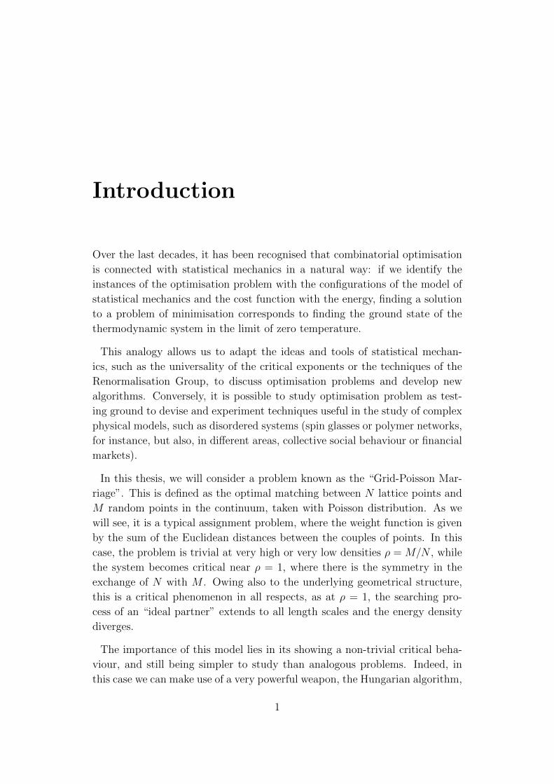
Figure 2.1: An example of a simple random walk of 200 steps in dimension 1.
interarrival process. If all r.v.’s Zn are independent and identically distributed,
then ZN , n ≥ 0 is called a renewal process or a recurrent process. From
Eq. (2.8), we see that
Tn = Z1 + Z2 + · · ·+ Zn (2.9)
where Tn denotes the time from the beginning until the occurrence of the nth
event. Thus, Tn, n ≥ 0 is sometimes called an arrival process.
A continuous-time stochastic process X(t), t ≥ 0 with values in the state
space Ω = (0, 1, 2, . . . ) is called a counting process if X(t), for any t, represents
the total number of “events” that have occurred during the time period [0, t].
A counting process X(t), t ≥ 0 is said to be a Poisson process with rate
λ > 0 if:
1. X(0) = 0
2. X(t) is a process with independent increments
3. the number of events in any interval of length t is Poisson distributed
with rate λt, that is, for all s, t ≥ 0,
PX(t+ s)−X(s) = x = e−λt(λt)x
x!, x = 0, 1, 2, . . . (2.10)
Equivalently2, a counting process X(t), t ≥ 0 is said to be a Poisson process
with rate λ > 0 if:
2For a proof, see e.g. [8]

22 CHAPTER 2. THE GRID-POISSON MARRIAGE
1. X(0) = 0
2. X(t) is a process with independent and stationary increments
3. the following relations hold:
PX(t+ h)−X(t) = 1 = Xh+ o(h) (2.11)
PX(t+ h)−X(t) ≥ 2 = o(h), (2.12)
(where a function f(x) is said to be of order o(h) if limh→0 f(h)/h = 0.)
It is possible to show that if X(t), t ≥ 0 is a Poisson process with rate
λ, the corresponding sequence of successive interarrival times tn, n ≥ 1 are
independent identically distributed r.v.’s obeying an exponential density with
mean λ−1. The proof is given, e.g., in [8], but it is straightforward to see that
the probability law for first interarrival time is
Pt1 > τ = PX(τ) = 0 = e−λ (2.13)
as the event t1 > τ occurs if and only if no Poisson event has occurred in
the interval [0, t].
2.2.3 Point processes
The definition of our model relies on the concept of point process on a compact
subset of Rn.
Let E be a subset of Rn. We assume3 that Xn, n ≥ 0 are random elements
of E, which represent points in the state space E. Next, we define an indicator
random variable 1Xn by
1Xn(A) =
1, if Xn ∈ A
0, if Xn /∈ A(2.14)
Note, therefore, that 1Xn is a function whose domain is the subsets of E, and
whose range is 0, 1, and that it takes the value one whenever Xn is in the
subset of interest. Other common notations for an indicator random variable
are I and χ.
3Here, we are following [12]

2.3. THE MODEL 23
Next, we note that by taking the sum over n, we find the total number of
the points Xn contained in the set A. Therefore, we define the counting
measure N by
N :=∑n
1Xn (2.15)
so that for A ⊂ E,
N(A) :=∑n
1Xn(A) (2.16)
gives the total number of points in A ⊂ E.
The function N is called a point process, and Xn are called the points. If
the Xn’s are almost surely distinct, then the point process is known as simple.
We note that as N depends explicitly on the values of the points, Xn, it is
natural to call such an object a random measure.
We will make the running assumption that bounded regions of A must always
contain a finite number of points with a probability of one. That is, for any
bounded set A, PN(A) <∞ = 1.
The simplest example of a point process (and the one that will be used in
our work) is the Poisson point process, which is a spatial generalisation of the
Poisson process described above. Namely, we say that a point process N is a
(homogeneous) Poisson point process or a Poisson random measure if the joint
distributions of the counts N(Ai) on bounded disjoint sets Ai satisfy
P [N(Ai) = ki, i = 1, . . . n] =∏i
e−λµ(Ai)(λµ(Ai))
ki
ki!. (2.17)
where k1, . . . , kn are non-negative integers and µ denotes the Lebesgue meas-
ure. The constant λ is called the intensity or rate of the Poisson point process.
An inhomogeneous Poisson point process is defined as above but by replacing
λµ(Ai) with∫Aiλ(x)dx where λ is a non-negative function on Rd.
2.3 The model
Consider the hypercube4 [0, L]d ⊂ Rd, with L ∈ Z+, with the Euclidean
distance dist(a, b) = [(xb1 − xa1)2 + (xb2 − xa2)2 + . . .+ (xbd − xad)2]1/2.
4Note that, in this work, d will either be 1 or 2, therefore we will consider only intervalsin R or squares on the plane.

24 CHAPTER 2. THE GRID-POISSON MARRIAGE
We will call grid points the discrete subset of points of the hypercube, defined
by
G = (i1−0.5, i2−0.5, . . . , id−0.5) ∈ [0, L]d,with ik = 1, 2, . . . , L (2.18)
The number of grid points is N = |G| = Ld.
Let P be a simple point process of finite intensity ρ in [0, L]d. The support
of P is the discrete random set
P := ~x ∈ Rd : P(~x) = 1. (2.19)
We define P as an instance of Poisson points. The coordinates of the Pois-
son points are independent and identically distributed random variables with
uniform distribution in [0, L].
We define M as the number of Poisson points, M = |P|.
Figure 2.2: Left: grid points on the square [0, L]× [0, L], with L = 12. Right:an example of an instance of 144 Poisson points on the same square.
Given an instance of Poisson points, we define a marriage between grid and
Poisson points as a function π : G ′ ⊂ G −→ P , with |G ′| = min(N,M), that
matches a grid point to a Poisson point, in such a way that every Poisson
point is “married” to no more than one grid point. In the terminology of
graph theory, a marriage is a maximum bipartite matching between G and P(i.e. a maximum matching of G ∪ P where all the edges are from G to P).

2.3. THE MODEL 25
We define a weight function on the edges of the matching as the length of
the edge. The energy associated with a marriage π is then defined as the sum
of the distances between matched pairs:
HP(π) :=N∑i=1
dist(i, π(i)) (2.20)
We will call πopt the marriage with minimum energy and we define the energy
(or cost) of an instance of Poisson points as the energy of πopt
H(P) := HP(πopt) = minπHP(π) (2.21)
If the instance has a single marriage π with minimum energy, we say that it
is non-degenerate, otherwise it is degenerate.
Again, if we consider the complete bipartite, this time weighed, graph KN,M ,
with V (KN,M) = G ∪P and weight function w(i, j) = dist(i, j), what we want
to find is the optimal maximum matching of KN,M .
Figure 2.3: The optimal marriage for the points in Fig. 2.2.
On the other hand, in the lexicon of combinatorial optimisation, the GPM is
a particular case of assignment problem. The space of possible configurations

26 CHAPTER 2. THE GRID-POISSON MARRIAGE
is the set of all possible marriages (if |G| = |P| = N , the number of possible
marriages is N !), and the cost function to minimise is the energy HP(π).
However, in this case, the costs εij are not independent from each other, as
they were in the problem job-workers, and they cannot, for example, be chosen
randomly, but are subject to geometrical constraints. It is clear that, if A, B
an C are three points on the plane, then dist(A,B) cannot be independent
from dist(A,C) and dist(C,B). These constraints make it difficult to perform
statistical averages and prevent us from using powerful tools like mean field
theory or the cavity method. And not only does this make the analysis more
difficult, but also changes the characteristics of the problem. In the random
assignment problem, it has been shown [7] that as N →∞ the energy becomes
a constant, while, as we will see in Chap. 5, in the GPM (like in the Poisson-
Poisson marriage) the energy grows faster than the number of couples.

3The marriage problem in onedimension
3.1 Exact solution for the correlation function
at density one
We want to describe the characteristics of the optimal marriage on a linear
lattice at density ρ = 1.
In our numerical simulations, we can only have a discrete system with a
finite number of points. However, for simplicity of calculation, we deal with
the problem in the continuum limit, that is we imagine to take the lattice
spacing to zero while holding the density fixed. The real system will hopefully
tend to this model as the number of points increases.
With this premise in mind, we start by introducing some mathematical tools
we will need in our analysis.
3.1.1 Definitions
Wiener process
A standard one-dimensional Wiener process (also called Brownian motion pro-
cess, as it was first introduced to describe the natural phenomenon of the same
name) is a stochastic process W (t): t ∈ R, t ≥ 0, with the following properties:
(1) W (0) = 0
27

28 CHAPTER 3. THE MARRIAGE PROBLEM IN ONE DIMENSION
(2) The function t→ W (t) is almost surely continuous
(3) The process W (t) has stationary, independent increments
(4) The increment W (t) −W (s) is normally distributed with expected value
0 and variance t− s
Basic properties of the Wiener process
W (t) is a Gaussian process, that is for all n and times t1, . . . , tn, the
linear combination of W (t1), . . . ,W (tn) is normally distributed
The unconditional probability density function at a fixed time t is given
by
pW (t)(x) =1√2πt
e−x2
2t (3.1)
∀t, the expectation is zero:
E[W (t)] = 0 (3.2)
The variance:
var[W (t)] = E[W 2(t)]− E2[W (t)] = E[W 2(t)] = t (3.3)
The covariance1:
cov[W (s),W (t)] = min(s, t) (3.4)
The area of a Wiener process, defined by
W (−1)(t) :=
∫ t
0
dsW (s), (3.5)
1To see this, let us suppose s ≤ t. Then
cov[W (s),W (t)] = E[(W (s)− E[(W (s)]) · (W (t)− E[(W (t)])]
= E[W (s) ·W (t)] = E[W (s) · ((W (t)−W (s)) +W (s))]
= E[W (s) · (W (t)−W (s))] + E[W 2(s)] = s

3.1. EXACT SOLUTION FOR THE CORRELATION FUNCTION. . . 29
is itself a Wiener process (as a linear combination of Wiener processes) char-
acterised by its expected value and variance:
E[W (−1)(t)] =
∫ t
0
dsE[W (s)] = 0 (3.6)
var[W (−1)(t)] = E
[∫ t
0
ds
∫ t
0
ds′W (s)W (s′)
]=
∫ t
0
ds
∫ t
0
ds′ cov(Ws,W′s)
=
∫ t
0
ds
(∫ s
0
ds′ min(s, s′) +
∫ t
s
ds′ min(s, s′)
)=t3
3.
(3.7)
Brownian bridge
A standard Brownian bridge B(t) over the interval [0, 1] is a standard Wiener
process conditioned to have B(1) = B(0) = 0.
Now, if we have a Wiener process W (t), the linear combination
B(t) := W (t)− tW (1) (3.8)
is a Brownian bridge with expectation, variance and covariance:
E[B(t)] = 0 (3.9)
var[B(t)] = E[(W (t)− tW (1))2]
= E[W 2(t)]− 2tE[W (1) ·W (t)] + t2E[W 2(1)]
= t(1− t) (3.10)
cov[B(t), B(s)] = E[(W (t)− tW (1)) · (W (s)− sW (1))]
= min(t, s)− ts (3.11)
The area of a Brownian bridge, defined by
B(−1)(t) :=
∫ t
0
dsB(s), (3.12)
is, again, a Gaussian variable (as a linear combination of Wiener processes)
characterised by its expected value and variance:
E[B(−1)(t)] =
∫ t
0
dsE[B(s)] = 0 (3.13)

30 CHAPTER 3. THE MARRIAGE PROBLEM IN ONE DIMENSION
var[B(−1)(t)] =
∫ t
0
ds
∫ t
0
ds′ cov[B(s), B(s′)]
=
∫ t
0
ds
∫ t
0
ds′ (min(s, s′)− ss′)
=t3
3− t4
4. (3.14)
In particular, if t = 1,
var[B(−1)(1)] =1
12(3.15)
and the covariance between B(−1)(1) and B(t) is
cov[B(−1)(1), B(t)] =
∫ 1
0
ds cov[B(s), B(t)] =
∫ 1
0
ds (min(s, t)− st)
=1
2t(1− t). (3.16)
Let us consider two Brownian bridges, B(s) and B(t), and let us assume that
s ≤ t. The covariance matrix is then
C =
s(1− s) s(1− t)
s(1− t) t(1− t)
. (3.17)
The distribution is Gaussian, which means the density function is given by
pA(x1, x2) =√
detAe−
12
∑2i=1 xiAijxj
2π, (3.18)
with (see, for example, [9])
A = C−1 =
ts(t−s) − 1
t−s
− 1t−s
1−s(1−t)(t−s)
. (3.19)
3.1.2 Open boundary conditions
In our problem, we consider a linear lattice of size L and parameter 1, or,
equivalently, a linear lattice of size 1 and parameter 1/L, and we generate L
random points uniformly distributed on the interval [0, L] (equivalently, [0, 1]).

3.1. EXACT SOLUTION FOR THE CORRELATION FUNCTION. . . 31
In dimension one, for open boundary conditions, the optimal marriage is
a forced choice, as the first point of the grid must clearly be matched with
the first random point, the second with the second and so on. That is to
say, for all n, the nth point of the grid will be matched with the nth random
point and, as the random points are uniformly distributed, the (1-dimensional)
vector connecting the couple will be a random variable with zero mean and
variance = n.
In the limit L → ∞, this situation can be represented by a Wiener process
W (t). More precisely, as there are no points for t > 1, we can describe it as a
Brownian bridge B(t) over the interval [0, 1].
Figure 3.1: An example of Brownian bridge B(t) over the interval [0, 1] withintermediate times s and t
Now, let us consider two intermediate times, s and t, with 0 < s < t < 1.
The probability that the process started at the origin arrives at x after a time

32 CHAPTER 3. THE MARRIAGE PROBLEM IN ONE DIMENSION
s is Gaussian with zero mean and variance = s:
pW (s)(x) =1√2πs
e−x2
2s . (3.20)
Similarly, to move from x to y in the interval (t− s):
pW (t−s)(y − x) =1√
2π(t− s)e−
(y−x)22(t−s) (3.21)
and, finally, to move from y to 0 in the interval (1− t):
pW (1−t)(y) =1√
2π(1− t)e−
y2
2(1−t) . (3.22)
By a change of parameters, if we consider the three segments of length
a = sb = t− sc = 1− t,
(3.23)
the matrix A in (3.19) becomes
A =
1a
+ 1b−1b
−1b
1c
+ 1b
. (3.24)
In general, since the distribution is Gaussian, we know from (3.18) that
√detA
2π
∫ ∫dx dy e−
x2
2a− (x−y)2
2b− y
2
2c = 1, (3.25)
with
detA =a+ b+ c
abc. (3.26)
The joint probability distribution for the random variables x and y is then
pa,b,c(x, y) =√
2π√a+ b+ c
e−x2
2a− (x−y)2
2b− y
2
2c
√2πa√
2πb√
2πc. (3.27)

3.1. EXACT SOLUTION FOR THE CORRELATION FUNCTION. . . 33
Correlation function
Given an instance of Poisson points and found the optimal marriage as seen,
we can define the quantity ϕ(t) as the distance between the grid point in t and
the Poisson point associated to it by the marriage. If we define a correlation
function between two point s and t as
G1(s, t) =ϕ(s) · ϕ(t)
|ϕ(s)| · |ϕ(t)|, (3.28)
its value is obviously
G1(s, t) = sgn(ϕ(s)) · sgn(ϕ(t)) = sgn(ϕ(s) · ϕ(t)). (3.29)
Therefore, the quantity we want to calculate is the expected value of the sign
function under the measure (3.27). That is, with the substitution (3.23),
G2(a, b, c) =
∫ ∫dx dy pa,b,c(x, y) sgn(x · y)
=
∫ ∫dx dy
√2π√a+ b+ c
e−x2
2a− (x−y)2
2b− y
2
2c
√2πa√
2πb√
2πcsgn(x · y)
(3.30)
If we define
α(a, b, c) :=
∫x≥0
∫y≥0
dx dy pa,b,c(x, y) (3.31)
and
β(a, b, c) :=
∫x≥0
∫y≤0
dx dy pa,b,c(x, y), (3.32)
then
G2(a, b, c) = 2α(a, b, c)− 2β(a, b, c). (3.33)
In addition, since pa,b,c(x, y) is Gaussian, we know that
2α(a, b, c) + 2β(a, b, c) = 1, (3.34)
then
G2(a, b, c) = 4α(a, b, c)− 1. (3.35)

34 CHAPTER 3. THE MARRIAGE PROBLEM IN ONE DIMENSION
By performing the integral (3.31), we find
α(a, b, c) =1
4+
1
2πarctan
√ac
b(a+ b+ c), (3.36)
and then
G2(a, b, c) =2
πarctan
√ac
b(a+ b+ c), (3.37)
with, in this case,
a, b, c ≥ 0
a+ b+ c = 1.
(3.38)
If we keep the distance b between the two points constant, and we calculate
the mean over the interval [0, 1], we finally obtain
Gobc(b) =2
π
1
1− b
∫ 1−b
0
da arctan
√a(1− a− b)
b=
1−√b
1 +√b. (3.39)
Figure 3.2: The theoretical correlation function in one dimension for openboundary conditions.
3.1. EXACT SOLUTION FOR THE CORRELATION FUNCTION. . . 35
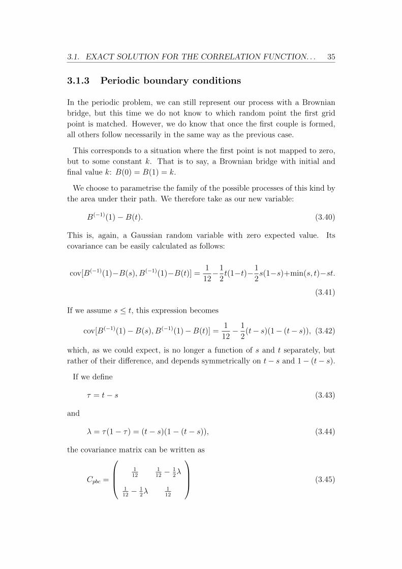
3.1.3 Periodic boundary conditions
In the periodic problem, we can still represent our process with a Brownian
bridge, but this time we do not know to which random point the first grid
point is matched. However, we do know that once the first couple is formed,
all others follow necessarily in the same way as the previous case.
This corresponds to a situation where the first point is not mapped to zero,
but to some constant k. That is to say, a Brownian bridge with initial and
final value k: B(0) = B(1) = k.
We choose to parametrise the family of the possible processes of this kind by
the area under their path. We therefore take as our new variable:
B(−1)(1)−B(t). (3.40)
This is, again, a Gaussian random variable with zero expected value. Its
covariance can be easily calculated as follows:
cov[B(−1)(1)−B(s), B(−1)(1)−B(t)] =1
12−1
2t(1−t)−1
2s(1−s)+min(s, t)−st.
(3.41)
If we assume s ≤ t, this expression becomes
cov[B(−1)(1)−B(s), B(−1)(1)−B(t)] =1
12− 1
2(t− s)(1− (t− s)), (3.42)
which, as we could expect, is no longer a function of s and t separately, but
rather of their difference, and depends symmetrically on t− s and 1− (t− s).
If we define
τ = t− s (3.43)
and
λ = τ(1− τ) = (t− s)(1− (t− s)), (3.44)
the covariance matrix can be written as
Cpbc =
112
112− 1
2λ
112− 1
2λ 1
12
(3.45)
36 CHAPTER 3. THE MARRIAGE PROBLEM IN ONE DIMENSION
and therefore
Apbc = C−1pbc =
1
λ(1− 3λ)
1 −1 + 6λ
−1 + 6λ 1
. (3.46)
By comparing (3.19) with (3.46), we find
b = λ(1−3λ)1−6λ
a = c = 1−3λ6.
(3.47)
The important difference with respect to the non-periodic case is that
a+ b+ c =(1− 3λ)2
3(1− 6λ), (3.48)
which is in general 6= 1. Moreover, b and a + b + c can now have a negative
sign:
b < 0a+ b+ c < 0
if λ >1
6. (3.49)
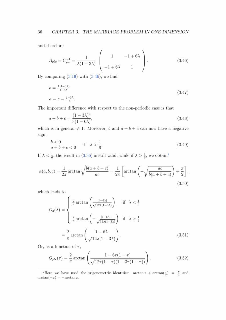
If λ < 16, the result in (3.36) is still valid, while if λ > 1
6, we obtain2
α(a, b, c) =1
2πarctan
√b(a+ b+ c)
ac=
1
2π
[arctan
(−√
ac
b(a+ b+ c)
)+π
2
],
(3.50)
which leads to
G3(λ) =
2π
arctan
(|1−6λ|√
12λ(1−3λ)
)if λ < 1
6
2π
arctan
(− |1−6λ|√
12λ(1−3λ)
)if λ > 1
6
=2
πarctan
(1− 6λ√
12λ(1− 3λ)
). (3.51)
Or, as a function of τ ,
Gpbc(τ) =2
πarctan
(1− 6τ(1− τ)√
12τ(1− τ)(1− 3τ(1− τ))
). (3.52)
2Here we have used the trigonometric identities: arctanx + arctan( 1x ) = π
2 andarctan(−x) = − arctanx.

3.2. NUMERICAL SIMULATIONS 37
Figure 3.3: The theoretical correlation function in one dimension for periodicboundary conditions.
3.2 Numerical simulations
3.2.1 Choice of the weight function
As we explained in Sect. 2.3, in two dimensions the optimal marriage we
have considered is the one which minimises the sum of the distances between
matched pairs.
However, in one dimension it was necessary to make a different choice and
minimise the sum of the squares of those distances. We had two reasons for
doing so.
The first is non-uniqueness in the definition of the optimal matching itself.
In one dimension, by using the distances as weights, it is far from exceptional
to meet with situations in which two or more matchings have the same energy,
that is, to have degenerate instances. To clarify this concept we have shown a
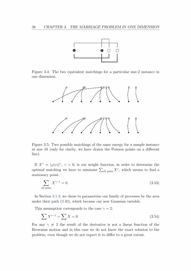
couple of examples in Figures 3.4 and 3.5.
Although this ambiguity itself does not affect the quantitative results for the
correlation function, it does affect other properties of the problem (such as the
distribution of the edge lengths, see Chap. 5).
The second and more important reason for minimising the sum of the squares
arises in the case of periodic boundary conditions and lies in the assumptions
we have made.
38 CHAPTER 3. THE MARRIAGE PROBLEM IN ONE DIMENSION
Figure 3.4: The two equivalent matchings for a particular size-2 instance inone dimension.
Figure 3.5: Two possible matchings of the same energy for a sample instanceat size 10 (only for clarity, we have drawn the Poisson points on a differentline).
If Xγ = |ϕ(x)|γ, γ > 0, is our weight function, in order to determine the
optimal matching we have to minimise∑
all pairsXγ, which means to find a
stationary point:∑all pairs
Xγ−1 = 0. (3.53)
In Section 3.1.3, we chose to parametrise our family of processes by the area
under their path (3.40), which became our new Gaussian variable.
This assumption corresponds to the case γ = 2:∑Xγ−1 =
∑X = 0 (3.54)
For any γ 6= 2 the result of the derivative is not a linear function of the
Brownian motion and in this case we do not know the exact solution to the
problem, even though we do not expect it to differ to a great extent.
3.2. NUMERICAL SIMULATIONS 39
3.2.2 Numerical results at the critical point
We show the results of our simulations for open (Fig. 3.6) and periodic (Fig. 3.7)
boundary conditions. The curves in colour represent the experimental data for
the correlation function, while the black ones are the plot of the theoretical
functions for different values of the system size.
We found that the experimental curves, both for open and periodic boundary
conditions, are in good agreement with the theoretical predictions, even at sizes
as small as L = 100.
Comparison for different weight functions
In Figure 3.8 we show the difference between the correlation function for the
optimal marriages obtained by minimising∑Xγ, with γ = 1, 2, 3, 4. We see
that the theoretical solution found is in agreement with experimental data for
γ = 2.
3.2.3 Near the critical point
We could not find an exact solution for the correlation function at ρ 6= 1 and
we do not have an ansatz on how it may be like. However, in Fig. 3.9 and
Fig. 3.10 we wish to show the qualitative behaviour of the curve as derived
from our simulations.
We see that both in the case of open and periodic boundary conditions, the
curves move up as the density increases, reach a peak at ρ = 1 and then move
down again.
Moreover, the shape and position of the curves are similar for the same value
of |t| = |ρ− 1|, regardless of the sign of t.
Finally, we observe that this function presents two ranges of behaviour. If
|t| < t, with t ≈ 0.01, the function is strictly decreasing with x, and has
a minimum at x = L, for open boundary conditions, or x = L2
fo periodic
bundary conditions. On the other hand, if |t| > t, the shape is different. It
reaches a minimum at an intermediate value x′, then goes up again approaching
zero as x→ L, or x→ L2
(depending on the boundary conditions).
If we define x as the point where the curve has a zero, we find that x(ρ) has
a maximum at density ρ = 1 (see Fig. 3.11).

40 CHAPTER 3. THE MARRIAGE PROBLEM IN ONE DIMENSION
Figure 3.6: The mean of the experimental correlation function over 104 in-stances of the optimal marriage in dimension one with open boundary con-ditions. Top: increasing sizes are represented from red (L = 100) to blue(L = 6500); Bottom: the same experimental curves, rescaled to show theagreement with the theoretical function, regardless of the size.
The value of xL/L at (t = 0) is known for all L, as in this case we have an

3.2. NUMERICAL SIMULATIONS 41
Figure 3.7: The mean of the experimental correlation function over 104 in-stances of the optimal marriage in dimension one with periodic boundary con-ditions. Top: increasing sizes are represented from red (L = 100) to blue(L = 6500); Bottom: the same experimental curves, rescaled to show theagreement with the theoretical function, regardless of the size.
exact solution.xL(t = 0)
L= 0.211325. (3.55)

42 CHAPTER 3. THE MARRIAGE PROBLEM IN ONE DIMENSION
Figure 3.8: Comparison of the correlation function at ρ = 1 for the optimalmarriages obtained by minimising
∑Xγ, with different values of γ (L = 5000).
From red to purple, γ = 1, 2, 3, 4 (green is γ = 2). Each curve is the meanover 103 instances of optimal marriage. The black thinner curve is the plot ofthe theoretical function.

3.2. NUMERICAL SIMULATIONS 43
Figure 3.9: The correlation function near the critical point at size 6000 withopen boundary conditions.Top: from red to cyan, ρ = 0.9, 0.91, 0.92, 0.93, 0.94, 0.95, 0.96, 0.97, 0.98,0.99, 0.991, 0.992, 0.993, 0.994, 0.995, 0.996, 0.997, 0.998, 0.999, 1.Bottom: from cyan to purple, ρ =1, 1.001, 1.002, 1.003, 1.004, 1.005, 1.006,1.007, 1.008, 1.009, 1.01, 1.02, 1.03, 1.04, 1.05, 1.06, 1.07, 1.08, 1.09, 1.1. Eachcurve is the mean over 103 instances of optimal marriage.

44 CHAPTER 3. THE MARRIAGE PROBLEM IN ONE DIMENSION
Figure 3.10: The correlation function near the critical point at size 6000 withperiodic boundary conditions.Top: from red to cyan, ρ = 0.9, 0.91, 0.92, 0.93, 0.94, 0.95, 0.96, 0.97, 0.98,0.99, 0.991, 0.992, 0.993, 0.994, 0.995, 0.996, 0.997, 0.998, 0.999, 1.Bottom: from cyan to purple, ρ =1, 1.001, 1.002, 1.003, 1.004, 1.005, 1.006,1.007, 1.008, 1.009, 1.01, 1.02, 1.03, 1.04, 1.05, 1.06, 1.07, 1.08, 1.09, 1.1. Eachcurve is the mean over 103 instances of optimal marriage.

3.2. NUMERICAL SIMULATIONS 45
Figure 3.11: The experimental rescaled intersection with the x-axis(xL/L) as a function of the density (ρ). From orange to blue, L =500, 1000, 2000, 3000, 4000, 6000. For all L, xL(t = 0)/L ≈ 0.211325.

46 CHAPTER 3. THE MARRIAGE PROBLEM IN ONE DIMENSION

4Finite-Size Scaling in twodimensions
Over the last decades, the widening availability of more and more powerful
computers and specially-designed processors has led to an ever-increasing role
of numerical simulations in studies of equilibrium and non-equilibrium prob-
lems of statistical mechanics.
In addition, it has become clear that for complex models such as those of
critical phenomena, analytic determinations are particularly difficult to achieve
and numerical results can bring about a great amount of useful qualitative and
quantitative information.
However, no matter how powerful the technology gets, computers will always
be able to deal only with a finite number of elements. Consequently, it is
possible to work only on lattices of finite sizes, while we know from statistical
mechanics that a phase transition can only occur in the thermodynamic limit,
that is, for systems where the number of particles tends to infinity.
Here comes into play the theory of finite-size scaling (FSS), which provides
a powerful technique to extrapolate to the thermodynamic limit from finite-
size results, which can be obtained from computer simulations. In this way
the behaviour of large systems can be inferred from the known behaviour of
relatively small systems.
The ideas of FSS were first introduced by Fisher [17], and Fisher and Barber
(see [14]), in the early seventies, and thoroughly studied in ensuing papers.
In the next section, we will give a brief introduction to the theory of FSS,
partly following [16]. Our description will be limited to the concepts necessary
to our purposes, while for a complete coverage and theoretical justification, we
refer to [13] and [14].
47

48 CHAPTER 4. FINITE-SIZE SCALING IN TWO DIMENSIONS
4.1 Theory of finite-size scaling
We shall consider the framework of second-order phase transitions, and a sys-
tem controlled by a single scalar parameter T (which is usually assimilated to
a temperature, while in our problem will correspond to a density).
4.1.1 Thermodynamic limit
We shall assume it is possible to give a thermodynamic description of our model
on a discrete lattice in a finite box Λ. That is to say, given any observable O,
we can calculate its value on the thermodynamic state determined by T and
Λ as
OΛ(T ) := 〈O〉Λ(T )
where 〈·〉Λ(T ) is the appropriate averaging. In addition, we shall assume the
existence of a thermodynamic limit. Usually, a model is taken to the ther-
modynamic limit by increasing the volume together with the particle number
while keeping the particle number density constant. A common way of doing
so is to consider an increasing sequence of boxes, Λnn. The value of the
observable in the infinite-volume is then given by
O∞ = limn→∞
OΛn(T )
This limit exists in a wide range of cases and usually does not depend on the
shape of the boxes. Only in the thermodynamic limit can the singularities
in the thermodynamic functions associated with a critical point occur. In
this case, in systems characterized by short-range interactions, if we define a
(connected) correlation function of the order parameter φ(x) as
Gφ,∞(x) := 〈φ(x);φ(0)〉∞ = 〈φ(0)φ(x)〉∞ − 〈φ(0)〉∞〈φ(x)〉∞,
we expect Gφ,∞(x) to show an exponential decay at long distances
Gφ,∞(x) ∼x→∞
e−|x|ξ∞
As we saw in Chap. 1, the length scale governing this exponential decay is
the correlation length ξ∞:
ξ∞ := − lim|x|→∞
|x|log |Gφ,∞(x)|

4.1. THEORY OF FINITE-SIZE SCALING 49
In principle, the correlation length may depend on the direction along wich
this limit is taken. However, for simplicity, in the following we shall only take
into consideration systems in which ξ does not depend on this direction and
are thus said to undergo an isotropic phase transition. In this case, we shall
consider boxes of size L in all directions. We shall also only consider the case
of zero external ordering field: H = 0.
4.1.2 Scaling hypothesis
In the proximity of the critical point at t = 0, where we have defined the
reduced temperature
t :=T − TcTc
(4.1)
(Tc being the critical temperature, at which the second-order phase transition
occurs), several thermodynamic quantities diverge. Their bulk (L = ∞) crit-
ical behaviour is given by
O∞(t) ∼ |t|−xO for t→ 0, (4.2)
where ∼ means that limt→0O∞(t)/|t|−xO is finite, and xO is the critical expo-
nent of O. As seen, the critical exponent of the correlation length is tradition-
ally denoted by ν:
ξ∞ ∼ |t|−ν for t→ 0, (4.3)
As we have already pointed out, a phase transition is only possible in the
thermodynamic limit, that is, for infinite volumes. This means that
limt→0
limL→∞
OL(t)/|t|−xO 6= limL→∞
limt→0OL(t)/|t|−xO = 0, (4.4)
if, for example, xO > 0.
The finite-size scaling theory predicts the behaviour of the function OL(t)
near Tc and for L large enough compared to the lattice spacing. In this region,
called the critical region, it is possible to write OL(t) as a function of ξ∞ and
L:
OL(t) ≈ fO(ξ∞(t), L),
where ≈ means that we are omitting lower-order terms as L→∞.

50 CHAPTER 4. FINITE-SIZE SCALING IN TWO DIMENSIONS
As ξ∞(t) and L are the only dimensionful quantities, the function fO(x, y)
must be a homogeneous function of its arguments, then
OL(t) ≈ fO(ξ∞(t), L) = ξ∞(t)yOF(1)O
(ξ∞(t)
L
)(4.5)
or, equivalently,
OL(t) ≈ LyOF(2)O
(ξ∞(t)
L
)(4.6)
The exponent yO, that is the degree of the homogeneous function, can be
determined as xO/ν, since1
O∞(t) = limL→∞
OL(t) = ξ∞(t)yOF(1)O (0) ∼ |t|−νyO
In this way, for a good definition of the finite-size correlation length, we must
have
ξL(t) ≈ L · g(ξ∞(t)
L
), (4.7)
since, in this case, xξ = ν.
4.1.3 Asymptotic form of FSS
At this point, we can replace the unknown quantity ξ∞ with known parameters
wich can be tuned in experiments: t and L.
OL(t) ≈ LxO/νF(2)O
(ξ∞(t)
L
)≈ LxO/νF
(2)O
(t−ν
L
)= LxO/νGO
(tL1/ν
)(4.8)
The function GO(z) is finite and non-vanishing in zero, and should satisfy
GO(z) ∼ |z|−xO for z →∞. (4.9)
This simple form of the FSS hypothesis heavily relies on the assumption that
the bulk critical temperature is known or can be evaluated. In addition, the
unknown critical exponent of ξ∞ is still present.
1We wish to point out that the existence of a finite limit for F(1)O (z) for z → 0 is based
on the hypotheses of the existence of a thermodynamic limit for OL and the possibility tointerchange this limit with the FSS limit. We will assume these are verified. For a deeperanalysis on this subject, we refer to [16].
4.1. THEORY OF FINITE-SIZE SCALING 51
An important consequence of (4.8) is that, once we get to know Tc, it tells
us that there is a well defined functional dependence between OL(t)/LxO/ν
and tL1/ν over the critical region. This suggests the possibility of estimating
xO and ν by carrying out experiments at different sizes and temperatures and
plotting the results with different values of the exponents until the set of points
collapse into a single curve.
4.1.4 Extrapolating to infinite volume
As explained in [15], there is another strategy to take advantage of FSS re-
lations in such a way as to obtain a relation which can be profitably used in
numerical experiments.
In the critical region, for any fixed t, (4.7) can be written as
ξLL≈ g
(ξ∞L
)or, by inverting the functional relation,
ξ∞L≈ h
(ξLL
). (4.10)
This means that
OL(t) ≈ LxO/νF(3)O
(ξL(t)
L
)(4.11)
and therefore, if we take the ratio of OL(t) at two different sizes L and αL, we
have
OαL(t)
OL(t)≈ FO
(ξL(t)
L
), (4.12)
where the critical exponents disappear and only measurable quantities of the
finite system are present.
In particular, this relation is valid for the correlation length. At fixed t
ξαL(t)
ξL(t)≈ Fξ
(ξL(t)
L
), (4.13)
As a result, we find that in a regime where FSS is proved to hold, there must be
a universal function which, if we are able to estimate it, allows us to extrapolate

52 CHAPTER 4. FINITE-SIZE SCALING IN TWO DIMENSIONS
values of ξαnL and OαnL for arbitrary n, until we get to the limiting values ξ∞and O∞ (save, of course, for systematic and statistical errors).
The idea is that we make numerical experiments at finite L and we want to
extrapolate to L→∞. However, we do not want to do so in some naıve way
(that is, simply extrapolating from a series of points), but we want to avail
ourselves of this structure. By doing so, we are really capable of extrapolating
to much larger values of L than we can simulate, and we are using a finer
approach.
Clearly, these expressions are not exact. The corrections can be evaluated
by means of the techniques of the Renormalization Group, but this is beyond
the scope of this work.
4.2 Numerical simulations
In the following, we will apply the FSS theory to the marriage problem in two
dimensions and verify whether the scaling relations (especially (4.8)) hold in
this context.
Firstly, we need to define the order parameter and the corresponding correl-
ation function we want to analyse.
4.2.1 Definitions
Let us consider the GPM problem on a square lattice of side L. Given an
instance of Poisson points and found the optimal marriage as seen (see 2.3),
we can define a map ~ϕ that relates each matched grid point of coordinates ~x
to a vector ~ϕ(~x) with the tail in ~x and the head in the matched Poisson point.
We then define a finite-size correlation function between two grid points ~x
and ~x′ as2
Gpp(~x, ~x′) =
~ϕ(~x) · ~ϕ(~x′)
|~ϕ(~x)| ·∣∣∣~ϕ(~x′)
∣∣∣ = cos θ(~ϕ(~x), ~ϕ(~x′)), (4.14)
2In the following, we will imply that we are taking the average over the probabilitydistribution of the Poisson points 〈·〉P . In concrete terms, we will be averaging over from103 to 5 · 104 instances of Poisson points.

4.2. NUMERICAL SIMULATIONS 53
(where θ(~ϕ, ~ϕ′
)is the angle between the two vectors), and a finite-size cor-
relation function at distance ~r:
G(~r) =
⟨~ϕ(~x) · ~ϕ(~x+ ~r)
|~ϕ(~x)| · |~ϕ(~x+ ~r)|
⟩~x
, (4.15)
where 〈·〉~x means we are taking the average over the coordinates ~x of all
matched grid points.
The wall-to-wall correlation function
In this work, we have focused our attention on the wall-to-wall correlation func-
tion, which describes the correlation of all points that belong to the columns
(rows) at a fixed horizontal (vertical) distance z (z ∈ [0, L− 1], z ∈ N).
More precisely, we define the horizontal wall-to-wall correlation function as
GhL(x, z) =
⟨~ϕ(x, y) · ~ϕ(x+ z, y′)
|~ϕ(x, y)| · |~ϕ(x+ z, y′)|
⟩yy′, (4.16)
where ~x = (x, y), and 〈·〉yy′ means we are taking the average over the vertical
coordinates y and y′ of the matched pairs in the columns.
In a more operative form
GhL(x, z) =
1
n
L∑y,y′=1
y,y′ of matched pairs
~ϕ(x, y) · ~ϕ(x+ z, y′)
|~ϕ(x, y)| · |~ϕ(x+ z, y′)|, (4.17)
where n = L2 if all grid points in the columns are matched.
The vertical wall-to-wall correlation function GvL(y, z) is defined equivalently.
The quantity we studied was the symmetrisation at distance z of the average
of the horizontal and vertical wall-to-wall function over all coordinates x and
y:
G(z, L) =1
2
(〈Gh
L(x, z)〉x + 〈GvL(y, z)〉y
)(4.18)
The reason why we chose to study this function, instead of (4.15) is that it
is easier to handle, as it is a function of only one integer variable.
In addition, we have decided to focus only on the case of periodic boundary
conditions (that is to say, on a torus), in order to avoid border effects.

54 CHAPTER 4. FINITE-SIZE SCALING IN TWO DIMENSIONS
Our function will then depend on two parameters, the side of lattice L and
the reduced temperature t = ρ−ρcρc
= ρ− 1, and one variable x.
Moreover, by construction, it will be symmetric in the exchange of x with
L− x:
G(x, L, t) = G(L− x, L, t) (4.19)
and consequently, only values of x in [0, L2] will be considered.
4.2.2 Qualitative behaviour of the correlation function
In Fig. 4.1, we show the behaviour of the curves for a sample side L = 60 at
different values of the parameter t.
Similarly to what we found in one dimension, we can see that there are
essentially two ranges of behaviour:
· if |t| < t, with t ≈ 0.01, the function is strictly decreasing with x, and
has a minimum at x = L2.
· if |t| > t, on the other hand, the shape is different. It reaches a minimum
at an intermediate value x′ (0 < x′ < L2), then goes up again and presents
a maximum at x = L2.
We are interested in the critical behaviour, that is, near t = 0. Therefore in
the following we will only consider the smallest values of |t|, where the curves
are of the first type.
Moreover, we see that the experimental value of G as we have defined it
is to some extent altered at x = 0 by the presence in the sum of the terms
of self-correlation, Gpp(~x, ~x) = 1, which raise abnormally the figure. For this
reason, in our following analyses, we will not consider this point.
By looking at the curves in Fig. 4.1 and Fig. 4.2, we also observe that, on
first approximation, the shape of the curve depends on the absolute value of
t, but is very similar for positive and negative signs.
As a last preliminary note, we see that the point of intersection of the curves
and the x-axis increases with t for t < 0, has a maximum at t = 0 and then
decreases with t for t > 0.

4.2. NUMERICAL SIMULATIONS 55
Figure 4.1: The wall-to-wall correlation function at side L = 60 for differentvalues of the density.Top: from red to cyan, ρ = 0.9, 0.91, 0.92, 0.93, 0.94, 0.95, 0.96, 0.97, 0.98,0.986, 0.99, 0.991, 0.992, 0.993, 0.994, 0.996, 0.997, 0.998, 0.999, 1.Bottom: from cyan to purple, ρ = 1, 1.001, 1.002, 1.003, 1.004, 1.006, 1.007,1.008, 1.009, 1.01, 1.015, 1.02, 1.03, 1.04, 1.05, 1.06, 1.07, 1.08, 1.09, 1.1.
4.2.3 Curve-fitting ansatz
We want to make an educated guess about what mathematical function can
describe the behaviour we expect from the system and be best in accordance

56 CHAPTER 4. FINITE-SIZE SCALING IN TWO DIMENSIONS
Figure 4.2: Comparison of the wall-to-wall correlation function at t =±0.001,±0.003,±0.006,±0.008 and t = ±0.01 (L = 60).
with the experimental data. In particular, we are looking for a function which
shows an exponential decay with the distance, x, but is symmetric in the
exchange x↔ L− x.
Our first choice is then the hyperbolic cosine:
G(x, L, t) = a · cosh
[c ·(x− L
2
)]+ b, (4.20)
where a = a(L, t), b = b(L, t) and c = c(L, t) are the fitting parameters we
would like to estimate.
For small values of |t|, t 6= 0, the experimental points are fitted well by this
function, as we show in Fig. 4.3.
On the contrary, at precisely t = 0 it has been impossible to find a clear fit
with the function (4.20), as the parameter c tends to vanish.
Since for small values of its argument, the hyperbolic cosine can be approx-
imated by a parabola, on the critical point we chose to fit our data to the
function:
G(x, L, t = 0) = a ·(x− L
2
)2
+ b, (4.21)
with a = a(L, t) and b = b(L, t) (see Fig. 4.4).

4.2. NUMERICAL SIMULATIONS 57
Figure 4.3: The experimental points for the correlation function for L = 60near t = 0 shown together with their respective fitted curves (hyperbolic co-sines).
Figure 4.4: The experimental points for the correlation function at t = 0shown together with the respective fitted curves (parabolas). From red topurple, L = 12, 16, 20, . . . , 96, 100.
58 CHAPTER 4. FINITE-SIZE SCALING IN TWO DIMENSIONS
We would like to observe that, similarly to what happened with the function
we found as an exact solution in one dimension with periodic boundary condi-
tions (see Sect. 3.1.3), in this context the dependence on the rescaled distancexL
is through an expression which depends symmetrically on xL
and (1− xL
), as
it is easily seen:(L
2− x)2
= L2
(1
4− x
L
(1− x
L
)), (4.22)
4.2.4 Scaling ansatz at the critical point
If t is small enough, theory tells us there must be scaling. This means that
G(x, L, t) must be a homogeneous function, for instance3:
G(x, L, t) ≈ LαF(xL, tL1/ν
)(4.23)
where, in the notation of the previous sections, α = xG/ν (cf (4.8)).
We are interested in knowing what the function F is like and the values of
the parameters α and ν. However, in this form, G can be difficult to study,
as it depends on two arguments. For this reason, in the first place, we have
studied the behaviour of this function at t = 0, as we do not meet with any
difficulties in performing simulations exactly on the critical point.
It is clear that, on first approximation, if t = 0,
G(x, L, t = 0) ≈ Lαf(xL
). (4.24)
where f(z) is a universal function.
4.2.5 Determination of the parameter α
We see that in (4.24) the exponent ν is no longer present. We can then focus
on finding an estimate for α.
3In general, F depends on x/Lβ , but we will see in the following that our simplifiedassumption in this case holds.

4.2. NUMERICAL SIMULATIONS 59
First estimate of α
A very simple way of determining the parameter α is the following. Let us
consider a certain fixed value of x such that G(x, L, t = 0) is not too close to
zero (any value, except x = 0 for the reason stated above). For instance, let
us take the point x = L2. We can therefore write
G(x =L
2, L, t = 0) ≈ Lαf
(1
2
). (4.25)
valid for all even L. Then
log
[−G
(L
2, L, 0
)]≈ log
[Lα(−f(
1
2
))]
≈ α logL+ log
[−f(
1
2
)](4.26)
In this way, if we plot log[−G
(L2, L, 0
)]against logL and calculate the
parameter of the linear fit (Fig. 4.5), this gives us a first rough estimate for α
as
α ≈ −0.176. (4.27)
In order to have an idea of the range of sides L in which this result is (ap-
proximately) correct, we plot G(L2, L, 0
)/Lα against L (see Fig. 4.6).
There are some fluctuations in these values, but for the time being we do not
see any well-defined systematic trends.
A preliminary test of our ansatz comes from the simple procedure of plotting
G (x, L, 0) /Lα as a function of xL
(see Fig. 4.7). As we hoped, all points collapse
into a single curve, regardless of the value of L. This curve is, as already seen
(Sect. 4.2.3), a parabola.
G(x, L, 0) = a(L) ·(x− L
2
)2
+ b(L) ≈ Lαf(xL
), (4.28)
which means that
f(xL
)≈ A
(x
L− 1
2
)2
+B, (4.29)

60 CHAPTER 4. FINITE-SIZE SCALING IN TWO DIMENSIONS
Figure 4.5: Plot of log[−G
(L2, L, 0
)]as a function of logL together with the
fitted line.
Figure 4.6: Plot of G(L2, L, 0
)/Lα as a function of L.
with a(L) = ALα−2 and b(L) = BLα.
There is a gap for small x and small L, which was expected and suggests it
can be appropriate to add some corrections to the (4.24).
It is important to observe that any estimate of α is affected by errors of two
different natures: statistical and systematic. The first component comes from

4.2. NUMERICAL SIMULATIONS 61
Figure 4.7: Plot of G (x, L, 0) /Lα as a function of x/L. In black, the plot of
f(x) = a ·(x− 1
2
)2+ b, with a = −0.06997 and b = 0.8452.
the statistical fluctuations that our points exhibit and it can be reduced by
making a larger number of simulations. The second component, on the other
hand, is due to the ansatz we are making about the formula. By using different
curves, we can try to better fit our data, and for this reason in the following
we will make some assumptions about the shape of f(xL
).
Ansatz on the corrections
The hypothesis we make on the form of the correction is the following:
G(x, L, 0) ≈ Lαf(xL
)+ Lα−2h
(xL
), (4.30)
First of all, we make a test at the point x = L/2.
G(L/2, L, 0) ≈ Lαf
(1
2
)+ Lα−2h
(1
2
)= Lα(B +QL−2), (4.31)
We found α = −0.1766, B = −0.07011 andQ = 0.01494. If we plotG(L/2, L, 0)
as a function of L with the fitted curve, we can verify whether our assumption
was correct (Fig. 4.8).

62 CHAPTER 4. FINITE-SIZE SCALING IN TWO DIMENSIONS
Figure 4.8: Plot of G(L2, L, 0
)against L for all L, together with the graph of
the fitted curve y(L) = Lα(B +QL−2), with α = −0.1766, B = −0.07011 andQ = 0.01494.
Investigation on the shape of the corrections
We want to make a basic estimate of the shape of h(xL
). In order to do so,
we fix the parameter α at the approximate value we have found in (4.27) and
consider G(x, L, 0) at different values of x = mL, m ∈(0, 1
2
]. For each m, we
take G(mL,L, 0) at different L (those L such that mL is integer) and make a
fit
G(mL,L, 0) = aLα + bLα−2 (4.32)
where the fit parameters we are computing are the values of f and h at the
point m.
Finally, we plot the results so obtained as m changes and examine the graphs
(Fig. 4.9 and Fig. 4.10).
For f(m), we find again the parabola we expected (Fig. 4.9), while the graph
obtained for h(m) is as shown in Fig. 4.10. We see that these points also lie
approximately on a curve of the shape of a parabola having vertex at m = 12.
We then write
f(xL
)= A
(x
L− 1
2
)2
+B (4.33)
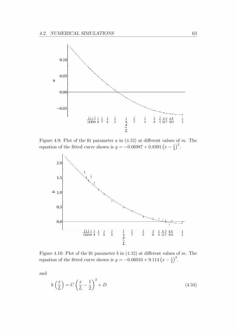
4.2. NUMERICAL SIMULATIONS 63
Figure 4.9: Plot of the fit parameter a in (4.32) at different values of m. The
equation of the fitted curve shown is y = −0.06987 + 0.8391(x− 1
2
)2.
Figure 4.10: Plot of the fit parameter b in (4.32) at different values of m. The
equation of the fitted curve shown is y = −0.06010 + 9.114(x− 1
2
)2.
and
h(xL
)= C
(x
L− 1
2
)2
+D (4.34)

64 CHAPTER 4. FINITE-SIZE SCALING IN TWO DIMENSIONS
Final ansatz on the form of the correlation function and calculationof the fit parameters
At this stage, we can write a second ansatz that takes into account the previous
correction.
G(x, L, 0) ≈ Lαf(xL
)+ Lα−2h
(xL
)≈ Lα
[A
(x
L− 1
2
)2
+B + L−2
(C
(x
L− 1
2
)2
+D
)].
(4.35)
In order to get the best estimate for all parameters at play in (4.35), the
last step is to put together all the information gathered so far and make a
non-linear fit for our correlation function with all available data, that is for all
x and L.
In Tab. 4.1, we present the values obtained from the fit with the two func-
tions:
f1
(xL
)= Lα
[A
(x
L− 1
2
)2
+B
](4.36)
f2
(xL
)= Lα
[A
(x
L− 1
2
)2
+B + L−2
(C
(x
L− 1
2
)2
+D
)](4.37)
with their respective χ2 tests.
The data we have analysed come from simulations on 5 · 104 instances of
optimal marriage for all L, 10 ≤ L ≤ 80, and 2 · 104 instances for all L,
81 ≤ L ≤ 102.
Our final estimate of the parameter α is then
α = −0.1752± 0.0003. (4.38)
In Fig. 4.11 we show the three-dimensional plot of the points at all x and
L (blue), together with the graph of the fitted curves for the two functions
considered (red).

4.2. NUMERICAL SIMULATIONS 65
f1 f2
α −0.1862± 0.00016 −0.1752± 0.0003
A 0.8805± 0.0006 0.837± 0.001
B −0.07294± 0.00005 −0.0697± 0.0001
C – 10.2± 0.1
D – −0.12± 0.01
χ2 18.73 2.63
Table 4.1: Table of the fit parameters for the functions in (4.36) and (4.37).
4.2.6 Behaviour near the critical point: definition andstudy of the correlation length
We want to give a good definition of the correlation length ξL at finite size
L and analyse its behaviour in the proximity of the critical point in order to
verify whether the FSS relations hold.
The first candidate of a correlation length we have examined is the inverse of
the fit parameter c in the equation of the correlation function as a hyperbolic
cosine:
G(x, L, t) = a · cosh
[c ·(x− L
2
)]+ b (4.39)
where a = a(L, t), b = b(L, t) and c = c(L, t).
ξ1(L, t) = (c(L, t))−1 (4.40)
As we observed, this definition is not applicable at t = 0 since the parameter
c tend to vanish as the curve becomes a parabola, and then a different approach
becomes necessary.
No matter what definition we choose, the bulk correlation length must be
such as to diverge for t → ∞. Moreover, as explained in Sect. 4.1.4, we
can replace the dependence of a generic observable OL(t) on ξ∞(t) with the

66 CHAPTER 4. FINITE-SIZE SCALING IN TWO DIMENSIONS
Figure 4.11: 3-D plot of the points at all x and L (blue), together with thegraph of the fitted curves (red) for f1
(xL
)(top) and f2
(xL
)(bottom).

4.2. NUMERICAL SIMULATIONS 67
dependence on ξL(t), where ξL(t) is any appropriate correlation length at finite
size L.
We then observe that in all the experimental curves, there is one (and only
one) point x such that
G(x, L, t) = 0 (4.41)
If the scaling ansatz holds, (4.41) is equivalent to
F(x
L,ξ∞L
)= 0 (4.42)
or
F(x
L,ξLL
)= 0 (4.43)
That is, xL
is a function of ξ∞L
or ξLL
x
L= H
(ξ∞L
)= K
(ξLL
)(4.44)
and therefore we can take x as a definition of correlation length at finite size.
The value of x is determined in the following way. We select the experimental
point nearest to zero, one point to its immediate left and one point to its
immediate right. We then make a fit of these three points with a polynomial
of degree two and take the intersection of the resulting curve with the x-axis.
By making use of the value of x and some properties of the curves, we can
give another estimate of the correlation length 4.40, independent from the
fitted curve. We proceed as follows. We consider a slightly, but equivalent,
parametrisation of the function 4.39, that is:
G(x, L, t) = a
cosh
[1
ξ
(x− L
2
)]− b. (4.45)
We then observe that the curves have zero integral (we see this by analysing
the experimental data), then:∫ L
0
G(x, L, t) = a
[2
(sinh
L
2ξ
)ξ − bL
]= 0 (4.46)
and use this property to write
b =2ξ
Lsinh
L
2ξ. (4.47)

68 CHAPTER 4. FINITE-SIZE SCALING IN TWO DIMENSIONS
Moreover, we have defined x as the point where G(x, L, t) = 0, then
cosh
(x
ξ− L
2ξ
)= b, (4.48)
which leads to the new definition of correlation length ξ2:
ξ2(L, t) =
ξ | L
2− ξ arccosh
[2ξ
Lsinh
(L
2ξ
)]= x
(4.49)
In Fig. 4.12 we show the ratio between the two definitions of correlation
length. We see that they are approximately equivalent.
Figure 4.12: The ratio between ξ2 and ξ1 as a function of t. From red to purple,L = 20, 22, 24, 26, 28, 30, 32, 36, 40, 44, 48, 52, 56, 60, 64.
In Fig. 4.13 and Fig. 4.14 we show the dependence of x/L and L/ξ2 on t,
while in Fig. 4.15 we show the ratio between x(L, t) and ξ2(L, t).
At the critical point t = 0
In Fig. 4.16 we show x(t = 0)/L as a function of L. The correlation length is
a typical size of the problem and at t = 0 must diverge for L→∞. We found
that
x ∼ L for L→∞ (4.50)

4.2. NUMERICAL SIMULATIONS 69
Figure 4.13: x(L, t)/L as a function of t. From red to purple, L = 20, 22, 24,26, 28, 30, 32, 36, 40, 44, 48, 52, 56, 60, 64.
Moreover, we observe that as L tends to∞, the ratio x/L tends to a quantity
very close to the value of the intersection with the x-axis of the exact solution
at t = 0 in one dimension, as calculated in 3.1.3 (cf (3.55)).
x
L→ k =
xdim1
L= 0.211325 for L→∞ (4.51)
Near the critical point, t ∼ 0, t 6= 0
Firstly, we use the (4.10) to replace ξ∞/L with x/L in (4.6) and write
G(x, L, t) = LαFG
(x
L,x(L, t)
L
). (4.52)
Now we can look at what happens at x = L/2 by plotting G(L/2, L, t)/Lα
against x(L, t)/L, with α as calculated in Sect. 4.2.5. In Fig. 4.17 we see that
the points fall approximately on the same curve, regardless of L. There are
some fluctuations within the data for the same L at different t.
Next, following Eq. (4.8), we plot G(L/2, L, t)/Lα against tL1/ν for different
values of ν. When all points collapse into a single curve regardless of L, we

70 CHAPTER 4. FINITE-SIZE SCALING IN TWO DIMENSIONS
Figure 4.14: L/ξ2(L, t) as a function of t. From red to purple, L = 20, 22, 24,26, 28, 30, 32, 36, 40, 44, 48, 52, 56, 60, 64.
Figure 4.15: x(L, t)/ξ2(L, t) as a function of t. From red to blue, L = 20, 22,24, 26, 28, 30, 32, 36, 40, 44, 48, 52, 56, 60, 64.
have found the correct value of ν. The results are shown in Fig. 4.18 and seem

4.2. NUMERICAL SIMULATIONS 71
Figure 4.16: x(t = 0)/L as a function of L. The line shown is at k = 0.211325and represents the value of the intersection with the x-axis of the theoreticalcurve at t = 0 in one dimension.
Figure 4.17: G(L/2, L, t)/Lα as a function of x(L, t)/L. From red to blue, L =20, 22, 24, 26, 28, 30, 32, 36, 40, 44, 48, 52, 56, 60, 64.
to suggest a value of the critical exponent ν of
ν ≈ 1. (4.53)

72 CHAPTER 4. FINITE-SIZE SCALING IN TWO DIMENSIONS
Figure 4.18: G(L/2, L, t)/Lα as a function of tL1/ν , for different values of ν.From red to purple, L = 20, 22, 24, 26, 28, 30, 32, 36, 40, 44, 48, 52, 56, 60,64.
Another test to find ν is by plotting x/L as a function of tL1/ν , as (4.42) is
equivalent to
F( xL, tL1/ν
)= 0. (4.54)

4.2. NUMERICAL SIMULATIONS 73
We show the results in Fig. 4.19.
Figure 4.19: x/L as a function of tL1/ν , for different values of ν. From red toblue, L = 20, 22, 24, 26, 28, 30, 32, 36, 40, 44, 48, 52, 56, 60, 64.
Similarly, in Fig. 4.20, we show the plots of L/ξ2 = L/ξ2(L, t) as a function
of tL1/ν .

74 CHAPTER 4. FINITE-SIZE SCALING IN TWO DIMENSIONS
Figure 4.20: L/ξ2 as a function of tL1/ν , for different values of ν. From red toblue, L = 20, 22, 24, 26, 28, 30, 32, 36, 40, 44, 48, 52, 56, 60, 64.
We see that the data for x and ξ2 are still very noisy and this does not allow
us to extract from them useful information on the correlation length. Further
investigation is necessary in this area.

5Probability density of thedistance between matched pairs
In this chapter we shall give an overall phenomenological description of the
behaviour of the length of the vectors that link each grid point to its respective
matched Poisson point. That is to say, the quantity that in the previous
chapters was referred to as |~ϕ(~x)|. For simplicity, in the following we will
merely call it “X”:
X = |~ϕ(~x)| .
This problem has already been addressed theoretically (for example, by Hol-
royd et al. [19]) for a generic perfect matching (bipartite or not), and also for
the stable marriage and other matching schemes, while many papers have been
written on the mean distance between matched pairs (see below, Sect. 5.1.1).
Here, we will focus on a numerical analysis in the specific case of the optimal
marriage as described in Chap. 2.
All data presented come from samples of 103 instances of optimal marriage,
and, as a consequence of the large amount of information produced in our nu-
merical experiments, it would be difficult (and not very significant) to consider
every single value of the quantity X. For this reason we decided, instead, to
focus on the probability density function, and to do so by making a histogram
of our data.
In the following graphics, the point at x = X represents the number of
vectors whose module falls between X and X + ∆, where ∆ is the width of
the bins. In two dimensions, the width we considered was a hundredth of the
75

76 CHAPTER 5. PROBABILITY DENSITY OF THE DISTANCE...
lattice constant: ∆2 = 1/100, while in one dimension, where, as we shall see,
the edge lengths tend to fall in a wider interval, we had to take a bin width of
one tenth of the lattice constant: ∆1 = 1/10.
We also want to point out that, as already explained in Chap. 3, the optimal
marriage considered in one dimension is the one which minimises the sum of
the squares of the edge lengths, instead of the usual edge lengths.
5.1 Numerical results in two dimensions
5.1.1 At the critical point
In Fig. 5.1 we show the histogram of our measurements at density ρ = 1 for
different sizes L of the system with a bin width of ∆2 = 1/100. We also show
the cumulative distribution function, that is p(X > r) (Fig. 5.2).
Figure 5.1: Normalised histogram of the edge length at density ρ = 1. Fromred to purple, all L between 10 and 102.
We see that the distribution has a well-defined peak that typically falls
between 0.4 and 0.5 and does not seem to depend on the value of L (Fig. 5.3).

5.1. NUMERICAL RESULTS IN TWO DIMENSIONS 77
Figure 5.2: Cumulative distribution function. From red to purple, all Lbetween 10 and 102.
Figure 5.3: Position of the peak of the previous curves as a function of the sizeof the system L.
The distribution tends to widen as L increases, as can be estimated by the
growth of the mean value of X and the variance1 σ2 = 〈X2〉−〈X〉2. (Fig. 5.4).
Finally, we observe the presence of small bends in the curves at precise points.
1In order to get a more precise number, the mean values of X and X2 were calculatedas the average over every single measure of X, rather than from the histogram.

78 CHAPTER 5. PROBABILITY DENSITY OF THE DISTANCE...
Figure 5.4: Mean value of X, 〈X〉, and variance σ2 = 〈X2〉−〈X〉2 as a functionof the size of the system L.
They can be explained by the characteristics of the grid: the distance X =√i,
i ∈ Z+, corresponds to the position of another grid point, which is a strong
“attractor” for Poisson points in the immediate neighbourhood.
Mean edge length
Studying the mean edge length is clearly the same as studying the energy or,
in other words, the transportation cost of the matching, defined as
TN =i=N∑i=1
Xi, (5.1)
where N = L2, is the number of pairs, Xi is the edge length of the ith matched
pair, and, obviously, 〈X〉 = TN/N .
This problem has been profusely treated in the past (see, for example, [21],
[22], [23], [24], and, for the related problem of the minimax matching length,
[25]) and it has been proved ([21]) that, for N couples in the unit square, there
exist two constant c, C such that2,
c(N logN)1/2 < TN < C(N logN)1/2 (5.2)
or, equivalently,
〈X〉 = O(√
logN/N). (5.3)
2The proof is given for two collections of random points, instead of a set of random pointsand a set of grid points, but this changes only constant multiplicative factors, as shown in[22].

5.1. NUMERICAL RESULTS IN TWO DIMENSIONS 79
The above result is related to a 1 × 1 square. By rescaling to L × L, we can
finally write:
〈X〉 = O(√
logL2) (5.4)
In order to verify this assumptions, we made a fit of our experimental data
with f(L) = a√
logL2 + b. The result is
〈X〉 = 0.202√
logL2 + 0.216, (5.5)
and the fitted curve is shown in Fig. 5.5.
Figure 5.5: Mean value of X, 〈X〉, as a function of the size of the systemL, together with the fitted curve f(L) = a
√logL2 + b, with a = 0.202 and
b = 0.216.
Tail behaviour
We want to analyse how the probability density function p(X) decreases as X
increases. In order to do so, we take the logarithm of p(X) and examine the
resulting curves.
We see that, at some distance from the peak, the logarithm of the curve
becomes, on first approximation, a linear function of X:
log(pL(X)) = AL +BLX (5.6)

80 CHAPTER 5. PROBABILITY DENSITY OF THE DISTANCE...
Figure 5.6: Logarithm of the probability density, shown with the fitted lines.From red to purple, all L between 10 and 102.
In Fig. 5.6 we show the points together with the fitted lines.
At different sizes L, the slope of the line changes, and this can be quantit-
atively evaluated by considering the value of the parameter BL of the fitting
function y = AL + BLx, with y = log(pL(X)), x = X, and AL = A(L, ρ = 1),
BL = B(L, ρ = 1).
We found that, on first approximation, the behaviour of BL as a function of
L can be described by (see Fig. 5.7)
B(L, ρ = 1) = −C −D logL
L. (5.7)
with C = 1.290 and D = 6.58.
Similarly, for AL (see Fig. 5.8):
A(L, ρ = 1) = F +GlogL
L. (5.8)
with F = 0.388 and G = 7.83.
By taking into account both results, we found that, if X is far enough from
the position of the peak (X & 1.5), the probability density function behaves
approximately as
p(X,L, ρ = 1) = F ′L1L
(G−DX)e−CX . (5.9)

5.1. NUMERICAL RESULTS IN TWO DIMENSIONS 81
Figure 5.7: The fit parameter BL as a function of L with the fitted curveC +D log(L)/L, with C = 1.290 and D = 6.58.
Figure 5.8: The fit parameter AL as a function of L with the fitted curveF +G log(L)/L, with F = 0.388 and G = 7.83.
A fit of all available data with the function in (5.9) gives the following results
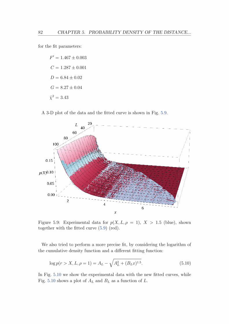
82 CHAPTER 5. PROBABILITY DENSITY OF THE DISTANCE...
for the fit parameters:
F ′ = 1.467± 0.003
C = 1.287± 0.001
D = 6.84± 0.02
G = 8.27± 0.04
χ2 = 3.43
A 3-D plot of the data and the fitted curve is shown in Fig. 5.9.
Figure 5.9: Experimental data for p(X,L, ρ = 1), X > 1.5 (blue), showntogether with the fitted curve (5.9) (red).
We also tried to perform a more precise fit, by considering the logarithm of
the cumulative density function and a different fitting function:
log p(r > X,L, ρ = 1) = AL −√A2L + (BLx)1.5. (5.10)
In Fig. 5.10 we show the experimental data with the new fitted curves, while
Fig. 5.10 shows a plot of AL and BL as a function of L.

5.1. NUMERICAL RESULTS IN TWO DIMENSIONS 83
Figure 5.10: Experimental data for log p(r > X,L, ρ = 1) (in colour), togetherwith the fitted curves (5.10) (black).
By plotting 1/AL and 1/BL as a function of logL (Fig. 5.10), we have estim-
ated:
1
AL= α0 + α1 logL (5.11)
1
BL
= β0 + β1 logL (5.12)
with α0 = −0.3233, α1 = 0.1537, β0 = −0.1247 and β1 = 0.0808 (Figures 5.11,
5.12 and 5.13).
Shape for small X
We want to have a closer look at the first points of the histogram, and try to
give a first estimate of the shape of the curves.
If we consider small distances from a certain grid point, we expect that,
if there is a Poisson point, probably it will be matched to the grid point
considered. As random points are distributed according to a Poisson point
process, if we consider the radial distribution we have
d p(rmin = r) = d r 2π r e−π r2
(5.13)

84 CHAPTER 5. PROBABILITY DENSITY OF THE DISTANCE...
Figure 5.11: 1/AL as a function of logL, with the fitted curve (5.11).
Figure 5.12: 1/BL as a function of logL, with the fitted curve (5.12).
and then we expect the cdf to be, on first approximation:
p(rmin > r) =
∫ ∞r
d r′ 2π r′ e−π r′2
= e−π r2
(5.14)
However, the situation described does not happen in all cases. If there are
many long edges, and one of them passes near the potential couple, it may be
energetically favourable to have two medium-length edges than a very small
and a very long one. If we look at Fig. 5.14, we see that the dashed-line
matching becomes preferable over the solid-line one when A+B+2ε > C+D,
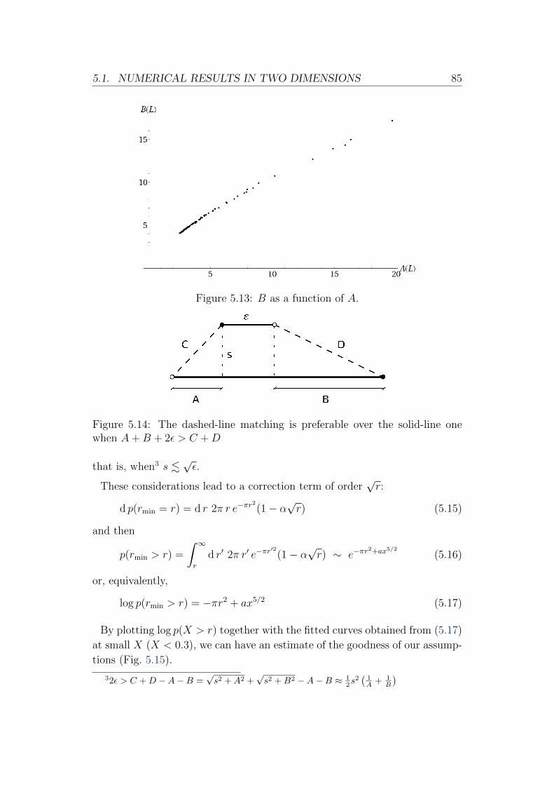
5.1. NUMERICAL RESULTS IN TWO DIMENSIONS 85
Figure 5.13: B as a function of A.
Figure 5.14: The dashed-line matching is preferable over the solid-line onewhen A+B + 2ε > C +D
that is, when3 s .√ε.
These considerations lead to a correction term of order√r:
d p(rmin = r) = d r 2π r e−πr2
(1− α√r) (5.15)
and then
p(rmin > r) =
∫ ∞r
d r′ 2π r′ e−πr′2
(1− α√r) ∼ e−πr
2+ax5/2 (5.16)
or, equivalently,
log p(rmin > r) = −πr2 + ax5/2 (5.17)
By plotting log p(X > r) together with the fitted curves obtained from (5.17)
at small X (X < 0.3), we can have an estimate of the goodness of our assump-
tions (Fig. 5.15).
32ε > C +D −A−B =√s2 +A2 +
√s2 +B2 −A−B ≈ 1
2s2(1A + 1
B
)

86 CHAPTER 5. PROBABILITY DENSITY OF THE DISTANCE...
In Fig. 5.16 we show a plot of the parameter a as a function of L. The fitted
curve shown is a(L) = b− c√
logLL
, with b = 2.872 and c = 3.045.
Figure 5.15: log p(X > r) with the fitted curves (5.17). In black, the plot ofy = −πr2.
Figure 5.16: The parameter a in (5.17) as a function of L with the fitted curve
a(L) = 2.872− 3.045√
logLL
.

5.1. NUMERICAL RESULTS IN TWO DIMENSIONS 87
5.1.2 Near the critical point
As the density ρ grows away from ρ = 1, we expect the distance between
matched points, on average, to decrease. For ρ 1, every grid point will
simply tend to be matched to the closest Poisson point, and the other way
round for ρ 1.
In Fig. 5.17 we show the probability density for the sample case L = 60 at
different values of the density ρ . We see that, as expected, the curves are more
Figure 5.17: pL=60,ρ(X), for different values of ρ. Top: from red to green, ρ =0.9, 0.91, 0.92, 0.93, 0.94, 0.95, 0.96, 0.97, 0.98, 0.986, 0.99, 0.991, 0.992, 0.993,0.994, 0.996, 0.997, 0.998, 0.999, 1.Bottom: from green to purple, ρ = 1, 1.001, 1.002, 1.003, 1.004, 1.006, 1.007,1.008, 1.009, 1.01, 1.016, 1.02, 1.03, 1.04, 1.05, 1.06, 1.07, 1.08, 1.09, 1.1.

88 CHAPTER 5. PROBABILITY DENSITY OF THE DISTANCE...
and more peaked as ρ grows away from 1. Moreover, if ρ > 1, the position of
the peak tends to get closer to zero as ρ increases (Fig. 5.18).
Figure 5.18: Position of the peak as a function of ρ (L=60).
Fig. 5.19 shows the mean and variance for X at different values of ρ, for
L = 60 fixed.
Figure 5.19: 〈X〉 (left) and σ2 = 〈X2〉−〈X〉2 (right) as a function of ρ (L=60).
The limit values we expect for 〈X〉 are4:
〈X〉 → 0 as ρ→∞
〈X〉 → 0.3825 as ρ→ 0.
To test this property we computed the mean value of X at L = 10, for different
densities from ρ = 0.01 to ρ = 110. The results are shown in Fig. 5.20.
4In the limit of one Poisson point in the lattice, the nearest grid point will be, on average,
at distance∫ 1/2
−1/2∫ 1/2
−1/2 dx dy√x2 + y2 = 0.3825.

5.1. NUMERICAL RESULTS IN TWO DIMENSIONS 89
Figure 5.20: 〈X〉 as a function of ρ. Left: ρ from 0.01 to 2. Right: ρ from 1to 110.
Tail behaviour
Also in this case, we examine the logarithm of the curves for X & 1.5 and we
make a fit with a line y = Aρ + Bρx, with y = log(pρ(X)), x = X. This time
L = L is fixed and Aρ = A(L, ρ), Bρ = B(L, ρ).
If we plot the values of the fit parameters as a function of ρ, we see that, on
first approximation, both AL=L(ρ) and BL=L(ρ) can be fitted by a polynomial
of degree 2 in the module of the reduced temperature |t| = |ρ−1|. In Fig. 5.22
we show the fitted curves for, as an example, L = 60.
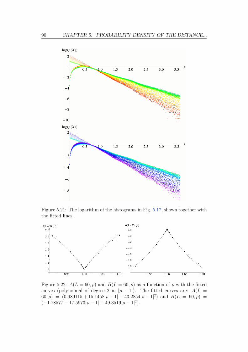
90 CHAPTER 5. PROBABILITY DENSITY OF THE DISTANCE...
Figure 5.21: The logarithm of the histograms in Fig. 5.17, shown together withthe fitted lines.
Figure 5.22: A(L = 60, ρ) and B(L = 60, ρ) as a function of ρ with the fittedcurves (polynomial of degree 2 in |ρ − 1|). The fitted curves are: A(L =60, ρ) = (0.989115 + 15.1458|ρ− 1| − 43.2854|ρ− 1|2) and B(L = 60, ρ) =(−1.78577− 17.5973|ρ− 1|+ 49.3519|ρ− 1|2).

5.2. NUMERICAL RESULTS IN ONE DIMENSION 91
5.2 Numerical results in one dimension
As previously mentioned, we found that in one dimension the distribution of
the lengths between matched points is considerably larger than in two dimen-
sions. For this reason, in this case we shall consider a broader histogram bin,
specifically, one tenth of the lattice parameter: ∆1 = 1/10. In addition, we
observe that these results have been obtained by minimising the sum of the
squares of the distance between matched pairs.
5.2.1 At the critical point
In Figures 5.23 and 5.24 we show the experimental curves at density ρ = 1 for
different sizes of the system. Again, the distribution tends to widen as the
Figure 5.23: Normalised histograms of the edge length at density ρ = 1. Fromred to purple, L =100, 200, 300, 400, 500, 600, 700, 800, 900, 1000, 1500, 2000,2500, 3000, 3500, 4000, 4500, 5000, 5500, 6000, 6500.
size, L, increases (in Fig. 5.25, 〈X〉 and σ2), while we cannot determine with
precision the position of the peak, as it appears to fall in the first bin of the
histogram. It may be possible to establish its value by considering narrower
bins.

92 CHAPTER 5. PROBABILITY DENSITY OF THE DISTANCE...
Figure 5.24: Cumulative distribution function. From red to purple, L between100 and 6500.
Figure 5.25: Mean value of X and variance σ2 = 〈X2〉 − 〈X〉2 as a function ofthe size of the system L.
Tail behaviour
Similarly to what we did in 2 dimensions, we take the logarithm of the prob-
ability density, but this time we find a different behaviour (Fig. 5.26).
Therefore, we try taking the squares of the abscissas, and in this way the
resulting curves become linear functions of X2 (Fig. 5.27):
log(pL(X)) = AL +BLX2 (5.18)
In Fig. 5.28. we show a plot of A(L) and B(L) as a function of L. This time
we could not find a suitable function to fit these points.

5.2. NUMERICAL RESULTS IN ONE DIMENSION 93
Figure 5.26: Logarithm of the probability distribution. From red to purple,L =100, 200, 300, 400, 500, 600, 700, 800, 900, 1000, 1500, 2000, 2500, 3000,3500, 4000, 4500, 5000, 5500, 6000, 6500.
Figure 5.27: Logarithm of the probability distribution as a function of X2.

94 CHAPTER 5. PROBABILITY DENSITY OF THE DISTANCE...
Figure 5.28: The fit parameters AL and BL in log pL(X) = AL + BLX2 as a
function of L.
5.2.2 Near the critical point
The comments we made for two dimensions hold also in one, and we expect the
mean edge length to decrease and the curves to narrow as the density grows
farther from ρ = 1 (see Fig. 5.29). In this case, the limit values we expect for
Figure 5.29: 〈X〉 (left) and σ2 = 〈X2〉 − 〈X〉2 (right) as a function of ρ(L=4000).
the mean edge length are:
〈X〉 → 0 as ρ→∞
〈X〉 → 0.25 as ρ→ 0,
as we have verified in Fig. 5.30.
In Fig. 5.31 we show the probability density for the sample case L = 4000
at different values of the density ρ, with 0.8 < ρ < 1.2. We then focus only
on the values closest to the critical point: 0.99 < ρ < 1.01 (Fig. 5.32). We
see that, as expected, the curves are more and more peaked as ρ grows away
from 1.

5.2. NUMERICAL RESULTS IN ONE DIMENSION 95
Figure 5.30: 〈X〉 as a function of ρ for L = 100. Left: ρ from 0.01 to 2. Right:ρ from 1 to 92.5.
Fig. 5.33 shows the logarithm of the previous curves and, similarly to what
already done at ρ = 1, by taking the squares of the abscissas, the resulting
curves become linear functions of X2 (Fig. 5.34):
Finally, in Fig. 5.35 we plot the values of the fit parameters and we find that,
again, they seem to be approximately a function of |t| = |ρ− 1|, even though
the dependence is significantly less precise than in the previous case.

96 CHAPTER 5. PROBABILITY DENSITY OF THE DISTANCE...
Figure 5.31: pL=4000,ρ(X), at different values of ρ. Top: from red to green,ρ = 0.8, 0.85, 0.9, 0.91, 0.92, 0.93, 0.94, 0.95, 0.96, 0.97, 0.98, 0.99, 0.991,0.992, 0.993, 0.994, 0.995, 0.996, 0.997, 0.998, 0.999, 1. Bottom: from green topurple, ρ = 1.001, 1.002, 1.003, 1.004, 1.005, 1.006, 1.007, 1.008, 1.009, 1.01,1.02, 1.03, 1.04, 1.05, 1.06, 1.07, 1.08, 1.09, 1.1, 1.15, 1.2.

5.2. NUMERICAL RESULTS IN ONE DIMENSION 97
Figure 5.32: pL=4000,ρ(X), at different values of ρ. From red to green, ρ = 0.99,0.991, 0.992, 0.993, 0.994, 0.995, 0.996, 0.997, 0.998, 0.999, 1. From green topurple, ρ = 1, 1.001, 1.002, 1.003, 1.004, 1.005, 1.006, 1.007, 1.008, 1.009, 1.01.
Figure 5.33: Logarithm of the curves above.

98 CHAPTER 5. PROBABILITY DENSITY OF THE DISTANCE...
Figure 5.34: Logarithm of the probability distribution as a function of X2,together with the fitted lines.
Figure 5.35: The fit parameters A = A(L, ρ) andB = B(L, ρ) for log(pL(X)) =A+BX2 as a function of ρ (L = 4000 fixed).

Conclusions and futuredevelopments
In this thesis, we have focused in particular on the behaviour of the Grid-
Poisson Marriage on the critical point, that is at ρ = 1.
Regarding the study of the correlation function, we have arrived at the exact
solution in one dimension at ρ = 1, and, by means of the theory of Finite-
Size Scaling, we have given an estimate of how this function scales in two
dimensions.
The results at ρ 6= 1, are less definite, particularly in one dimension, where
we do not have an ansatz for the form of the correlation function.
In two dimensions, despite having such an ansatz, the numerical simulations
have not enabled us to have precise numeric details on the correlation length,
which would have allowed us to use more sophisticated techniques for the
determination of the critical exponents.
In this sense, the question of a definition of correlation function convenient
from the point of view of a numerical determination, is still open to new ideas
and research.
Concerning the study of the length of the edges of the optimal matching, the
theoretical predictions about the mean value have been confirmed numerically,
to the best of our knowledge, for the first time, and we have come to an estimate
of the scaling of the energy with the number of couples for the two-dimensional
GPM on the critical point.
We have also given a preliminary description of the density distribution,
whose characteristics still need to be further investigated.
In conclusion, in this work the tools of statistical mechanics, and in particular
the techniques of the Finite-Size Scaling, have been profitably put into use in
the study of a problem of combinatorial optimisation, so confirming the strong
link between these two areas of study.
99


ATechnical tools
As the backbone of our work was the computer simulations we devised to
examine the statistical properties of our model, in this appendix we wish to
give a brief description of the main technical tools we have used.
We also want to point out that all the simulations performed for this thesis,
including the necessary tests and inevitable dead ends, add up to 233800 hours
of CPU process time.
A.1 Hardware
We were only able to carry out this large number of complex simulations thanks
to the facilities of the Laboratorio di Calcolo e Multimedia, that is to say, the
computer laboratory of the Physics Department of the University of Milan.
We could make use of a cluster of 13 client machines and a main server,
which performs two kinds of services: networking and computing1.
Networking services
NFS/Cluster diskless-root – The operating system is not present on the
client nodes. Instead, it is mounted remotely through the Network File
System protocol.
1The following information has been kindly provided by S. Mandelli, staff member of thelaboratory.
101

102 APPENDIX A. TECHNICAL TOOLS
DHCP – The Dynamic Host Configuration Protocol is used to assign an
IP address to any client that makes a request.
PXE – The Preboot eXecution Environment enables the server to re-
motely provide the clients with the kernel they need in order to boot.
BIND – The DNS server is needed to resolve the names of the nodes into
their IP addresses.
Computing services
PBS – The Portable Batch System is a service that performs job schedul-
ing. This task is accomplished by means of two programs:
· Torque 3.0.4, a distributed resource manager providing control over
batch jobs and distributed nodes.
· Maui 3.3, a cluster job scheduler.
Recently, five nodes have been added to an InfiniBand (very high speed)
subnetwork in order to enhance the simulations with MPI/OpenMPI
(Message Passing Interface), which require the utilization of several nodes
in parallel.
General notes on the cluster
The operating system on both the server and the nodes is Debian Linux
Stable (Squeeze 6.0).
All nodes are Dell PowerEdge.
All processors are Intel Xeon. In particular, there are four X5650, while
the least powerful are some X5450.
On the whole, by summing up the resources of all nodes, we get
· number of CPUs: 208
· total memory (RAM): 293 GB

A.2. SOFTWARE 103
A.2 Software
The programs we run were written in the C programming language. As a
starting-point, we took the source files by Elia Zarinelli, whose work of thesis [1]
was the basis for our own, modifying them as it was necessary for our purposes.
This code makes use in its core function of the implementation in C written
by Donald E. Knuth [3] of the Hungarian algorithm.
All data analyses and calculations have been performed by means of the
mathematical software program Wolfram Mathematica v. 8.0.
Finally, this thesis has been written using the LATEX 2ε typesetting system
and all original images have been created or modified either by the above-
mentioned Mathematica program or with the GIMP graphics editor.

104 APPENDIX A. TECHNICAL TOOLS

BBasic concepts of graph theory
B.1 Graphs and subgraphs
Let V be a finite set, and refer to the subsets of two (not necessarily distinct)
elements of V as
E(V ) = u, v|u, v ∈ V .
A pair G = (V,E) with E ⊆ E(V ) is called a graph (on V).
The elements of V are called the vertices (or nodes, or points) of G, and those
of E the edges (or lines, or arcs) of G.
We denote by V (G) the vertex set of G, and by E(G) the edge set. Their
cardinalities |V (G)| and |E(G)| are called, respectively, the order and the size
of the graph.
An edge with endvertices u and v is denoted by uv. The edge uv is said to
be incident to its ends u and v. Vertices u and v are adjacent or neighbours, if
uv ∈ G. If the endpoints are distinct, the edge is called a link, otherwise, it is
called a loop.
If the graph G contains loops vv and parallel (or multiple) edges between
vertices, it is called a multigraph, otherwise it is a simple graph.
In graphical representations, a vertex is usually drawn as a node or a dot,
while an edge is drawn as a line connecting two vertices.
If the pairs u, v are ordered (that is, E ⊆ V × V ), G(V,E) is called a
directed graph, or digraph. In this case, uv 6= vu. The directed edge is drawn
105
106 APPENDIX B. BASIC CONCEPTS OF GRAPH THEORY
as an arrow between the endpoints, and for this reason they are called the
tail and head of the edge. A digraph can contain edges uv and vu of opposite
directions.
Let v ∈ G be a vertex of a graph G. The neighbourhood of v is the set
NG(v) = u ∈ G|vu ∈ G.
The degree (or valency) of v is the number of its neighbours:
dG(v) = |NG(v)|.
If dG(v) = 0, then v is said to be isolated in G, and if dG(v) = 1, then v is a
leaf of the graph.
It is also possible to consider graphs with infinitely many vertices or edges
or both. In this case the graph is said to be infinite. An infinite graph where
every vertex has finite degree is called locally finite.
The graph G = KV is the complete graph on V, if every two vertices are
adjacent. All complete graphs of order n are isomorphic with each other, and
they are denoted by Kn.
A graph G is said to be regular, if every vertex of G has the same degree. If
this degree is equal to r, then G is r-regular or regular of degree r. A complete
graph Kn is (n− 1)-regular.
We can also we define a weight function w : E(G) → R, which assign a
“weight” ∈ R to each edge of the graph. In this case, we say that the graph is
(edge-)weighted.
A graph G is called bipartite, if VG has a partition to two subsets X and Y
such that each edge uv ∈ G connects a vertex of X and a vertex of Y . In this
case, G is said to be (X, Y )-bipartite.
A bipartite graph G is complete (m, k)-bipartite, if |X| = m, |Y | = k, and
uv ∈ G for all u ∈ X and v ∈ Y . All complete (m, k)-bipartite graphs are
isomorphic and denoted as Km,k.
A graph H is a subgraph of a graph G, denoted by H ⊆ G, if VH ⊆ VG and
EH ⊆ EG. A subgraph H ⊆ G spans G (and H is a spanning subgraph of G),
if every vertex of G is in H, that is, VH = VG.
For a graph G, a subset M ⊆ EG is a matching of G, if M contains no
adjacent edges. The two ends of an edge e ∈ M are matched under M . A
matching M is a maximum matching, if for no matching M ′, |M | < |M ′|.A matching M saturates v ∈ G, if v is an end of an edge in M . Also, M
saturates A ⊆ VG , if it saturates every v ∈ A. If M saturates VG , then M is
a perfect matching.

B.2. PATHS AND CYCLES 107
B.2 Paths and cycles
Let ei = uiui+1 ∈ G be (adjacent) edges of G for i ∈ [1, k]. The sequence
W = e1, e2, . . . ek is a walk of length k from u1 to uk+1.
W is said to be
· closed (or a loop), if u1 = uk+1
· a path, if ui 6= uj for all i 6= j
· a cycle, if it is closed, k ≥ 2, and ui 6= uj for i 6= j except that u1 = uk+1
A graph G is said to be connected, if for all u, v ∈ V (G), u and v can be
connected by a walk; otherwise, it is disconnected. The maximal connected
subgraphs of G are its connected components.
If we denote with c(G) the number of connected components of G, and with
L(G) the number of independent loops, then
|V (G)| − |E(G)|+ L(G) = c(G),
which is known as Euler’s formula.
A vertex v ∈ G is a cut vertex, if c(G−v) > c(G), that is, when it is removed
from G the graph becomes disconnected. Analogously, a cut edge or bridge is
an edge whose removal disconnects a graph.
A subset of arcs is called a cut if it is such that when these arcs are removed
from G, the graph becomes disconnected.
If a graph contains no cycles, it is said to be acyclic, or a forest. A connected
acyclic graph is a tree.

108 APPENDIX B. BASIC CONCEPTS OF GRAPH THEORY
CDistribution functions ofrandom variables
C.1 Distribution functions
Let X be a random variable.
The cumulative distribution function (cdf) of X is the function defined by
FX(x) = P (X ≤ x) −∞ < x <∞. (C.1)
We have
0 ≤ FX(x) ≤ 1
FX(x1) ≤ FX(x2) if x1 < x2
limx→∞
FX(x) = 1
limx→−∞
FX(x) = 0
limx→a+
FX(x) = FX(a)
P (a < X ≤ b) = FX(b)− FX(a)
P (X > a) = 1− FX(a)
P (X < b) = FX(b−) b− = lim0<ε→0
b− ε
Let X be a discrete random variable. If we define
pX(x) = P (X = x), (C.2)
pX(x) is called the probability mass function (pmf) of the discrete random
variable X, and
109

110APPENDIX C. DISTRIBUTION FUNCTIONS OF RANDOM
VARIABLES
0 ≤ pX(xk) ≤ 1 k = 1, 2, . . .
pX(x) = 0 if x 6= xk(k = 1, 2, . . .)
∑k
pX(xk) = 1
FX(x) = P (X ≤ x) =∑xk≤x
pX(xk)
Let X be a continuous r.v. and fX(x) =dFX(x)
dx. The function fX(x) is
called the probability density function (pdf) of X, and it has the following
properties
fX(x) ≥ 0
∞∫−∞
fX(x)dx = 1
fX(x) is piecewise continuous
FX(x) = P (X ≤ x) =x∫−∞
fX(x′)dx′
P (a < X ≤ b) =b∫a
fX(x)dx = FX(b)− FX(a)
Let ~X : Ω → Rd, ~X = (X1, X2, . . . , Xd). The (d-variate) distribution func-
tion of ~X or the joint distribution function of X1, X2, . . . , Xd is defined by
F (x1, . . . , xd) = PX1 ≤ x1, . . . , Xd ≤ xd (C.3)
for d ≥ 1, xk ∈ R, 1 ≤ k ≤ d.
If f(x1, . . . , xd) = ∂dF/(∂x1 . . . ∂xd) exists for all (x1, . . . , xd) ∈ Rd, then the
function f(x1, . . . , xd) is called the joint density function of F (x1, . . . , xd) or
(X1, X2, . . . , Xd), and
F (x1, . . . , xd) =
∫ x1
−∞. . .
∫ xd
−∞f(x′1, . . . , x
′d) dx
′d . . . dx
′1 (C.4)
C.2 Mean, variance and covariance
The mean (or expected value) of a r.v. X, denoted by µX or E[X], is
defined by
µX = E[X] =
∑
k xkpk(xk) X : discrete∫∞−∞ xfX(x)dx X : continuous
(C.5)

C.3. SOME SPECIAL DISTRIBUTIONS 111
The variance, denote by σ2X or var[X], is defined by
σ2X = var[X] = E[(X − E[X])2] (C.6)
and therefore
σ2X =
∑
k(xk − µk)2pk(xk) X : discrete∫∞−∞(x− µX)2fX(x)dx X : continuous
(C.7)
For any two random variables X and Y with finite variances σ2X and
σ2Y , the correlation of X and Y is defined by E[XY ], and the covariance
cov(X, Y ) is defined by
cov(X, Y ) = E[(X − µX)(Y − µY )] (C.8)
C.3 Some special distributions
Uniform distribution A r.v. X is called a uniform r.v. over the interval
(a, b) if its pdf is given by
fX(x) =
1b−a a < x < b
0 otherwise
(C.9)
Normal (or Gaussian) distribution A r.v. X is called a normal or Gaus-
sian r.v. if its pdf is given by
fX(x) =1√2πσ
e−(x−µ)2
2σ2 (C.10)
The mean and variance are
µX = E[X] = µ
σ2X = var[X] = σ2
It is customary to write N(µ;σ2) to denote a r.v. which is normal with
mean µ and variance σ2.
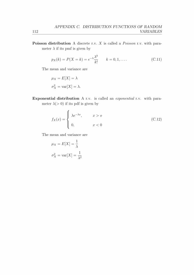
112APPENDIX C. DISTRIBUTION FUNCTIONS OF RANDOM
VARIABLES
Poisson distribution A discrete r.v. X is called a Poisson r.v. with para-
meter λ if its pmf is given by
pX(k) = P (X = k) = e−λλk
k!k = 0, 1, . . . . (C.11)
The mean and variance are
µX = E[X] = λ
σ2X = var[X] = λ.
Exponential distribution A r.v. is called an exponential r.v. with para-
meter λ(> 0) if its pdf is given by
fX(x) =
λe−λx, x > o
0, x < 0
(C.12)
The mean and variance are
µX = E[X] =1
λ
σ2X = var[X] =
1
λ2

Riassunto in italiano
Il lavoro svolto in questa tesi concerne le proprieta statistiche di un proble-
ma di ottimizzazione combinatoria conosciuto come “Grid-Poisson Marriage”
(GPM), ovvero il matching ottimale fra N punti di un reticolo e M punti scelti
a caso nel continuo con distribuzione Poissoniana.
Negli ultimi decenni si e compreso come i problemi di ottimizzazione sia-
no connessi a quelli di meccanica statistica in modo naturale: identificando
la funzione costo con l’energia, si tratta di trovare lo stato fondamentale a
temperatura nulla di un sistema a molti gradi di liberta. Questa analogia ci
permette di adattare le idee e gli strumenti della meccanica statistica, andando
nel limite di temperatura zero, al fine di affrontare problemi di ottimizzazione.
Il modello da noi considerato e un tipico problema di assegnazione in cui la
funzione peso e data dalla somma delle distanze euclidee fra le coppie di punti.
In questo caso, il problema e banale per densita ρ = M/N molto grandi o
molto piccole, mentre il sistema diventa critico intorno a ρ = 1, dove abbiamo
la simmetria nello scambio di N con M . Questo e un fenomeno critico a tutti
gli effetti, in quanto a ρ = 1 il processo di “ricerca del partner ideale” propaga
a tutte le scale di lunghezza e la densita di energia diverge.
In questa tesi abbiamo studiato alcune caratteristiche del GPM dal punto
di vista teorico e le abbiamo confrontate con i dati ottenuti da simulazioni
numeriche su reticoli di diverse taglie e con diverse densita di punti casuali.
Schema della tesi
Capitolo 1
Richiamiamo i concetti fondamentali di meccanica statistica e di ottimizzazione
combinatoria e spieghiamo il legame fra questi due ambiti di studio.
113

114 RIASSUNTO IN ITALIANO
Capitolo 2
Diamo le definizioni essenziali sui processi stocastici che ci serviranno nel
seguito e definiamo il modello oggetto di studio di questa tesi.
Capitolo 3
L’osservabile su cui ci concentriamo inizialmente e il versore che unisce i punti
accoppiati, mentre la funzione di correlazione che prendiamo in considerazione
e il loro prodotto scalare.
Per prima cosa, arriviamo alla soluzione esatta a densita ρ = 1 per la fun-
zione di correlazione in dimensione 1, che in questo caso si riduce al prodotto
dei segni. Modellizzando il comportamento del parametro d’ordine come un
ponte Browniano e mediando opportunamente sulla distribuzione di probabi-
lita cosı ricavata, otteniamo per la la funzione di correlazione G(x), nel caso
di condizioni al contorno aperte, l’espressione:
Gcca(x) =1−√x
1 +√x
mentre nel caso di condizioni al contorno periodiche:
Gccp(x) =2
πarctan
(1− 6x(1− x)√
12x(1− x)(1− 3x(1− x))
).
Consideriamo alcune variazioni della funzione peso e mostriamo come la so-
luzione analitica proposta sia in ottimo accordo con i risultati ottenuti dal-
le simulazioni numeriche, a patto di scegliere come funzione peso da mini-
mizzare la somma dei quadrati delle distanze fra i punti. Descriviamo poi
qualitativamente le curve numeriche nel caso ρ 6= 1.
Capitolo 4
Nel caso del GPM bidimensionale, applichiamo le idee fondamentali della teoria
del Finite-Size Scaling dei sistemi termodinamici allo studio della funzione di
correlazione wall-to-wall per scriverla come
G(x, L, t) ≈ LαF(xL, tL1/ν
),
dove L e la taglia del sistema e t = ρ− 1.

RIASSUNTO IN ITALIANO 115
Attraverso simulazioni sul punto critico t = 0, diamo una stima numerica del
valore di α.
Fuori dal punto critico, mostriamo numericamente l’andamento della funzio-
ne di correlazione. Diamo due possibili definizioni di lunghezza di correlazione
e ne esaminiamo il comportamento.
Capitolo 5
Infine, prendiamo in considerazione il modulo del vettore che unisce le coppie
e ne studiamo la distribuzione di probabilita ottenuta dalle simulazioni, per
diverse taglie del sistema e a diverse densita. Inoltre, esaminando la media 〈X〉di queste lunghezze in funzione della taglia del sistema, verifichiamo i risultati
presenti in letteratura: 〈X〉 = O(√
logN/N), che corrisponde a un andamento
dell’energia come: E = O(√N logN).

116 RIASSUNTO IN ITALIANO

Ringraziamenti
Primo fra tutti, vorrei ringraziare il Professor Caracciolo, non solo per tutto
cio che mi ha insegnato e su cui mi ha spinto a riflettere, ma anche per la sua
infinita gentilezza e pazienza, e per le molte parole di incoraggiamento che mi
ha rivolto nel corso di questi mesi.
Un ringraziamento particolare devo anche al Dottor Sportiello, per la sua
disponibilita, il suo competente aiuto e il suo contagioso entusiasmo.
Vorrei inoltre ringraziare Marco Gherardi per i suoi suggerimenti, e gli am-
ministratori del Laboratorio di Calcolo e Multimedia, in particolare Stefano
Mandelli e Roberto Palazzi, per l’assistenza che mi hanno fornito nell’utilizzo
della farm.
A livello personale, devo molto al supporto e all’incoraggiamento di alcune
persone. Fra questi, vorrei citare la mia cara amica Santa, che mi ha appog-
giato nei momenti difficili, e Monica e Roberto, con i quali ho condiviso molte
stimolanti conversazioni. Un grazie gigante anche a Tiziano, per il suo aiuto e
i suoi preziosi consigli.
Ultimi, ma non ultimi per importanza, ringrazio Simone per aver sopportato
cosı a lungo la mia lontananza, e i miei genitori, senza il supporto dei quali
non avrei potuto completare questo percorso.
117


Bibliography
[1] E. Zarinelli, Statistical properties of the random 2-dimensional euclidean
Grid-Poisson Marriage problem, Master’s Thesis, Universita degli Studi
di Milano, 2007-2008.
[2] D. Gale and L. Shapley, College admissions and stability of marriage,
Amer. Math. Monthly, 69(1): 9–15, 1962.
[3] D. E. Knuth, The Stanford GraphBase: A Platform for the Combinatorial
computing, Addison-Wesley, 1993.
[4] D. E. Knuth, Mariages Stables et leurs relations avec d’autres problemes
combinatoires, Montreal, Les Presses de l’Universite de Montreal, 1976.
[5] Gaspard Monge, Memoire sur la theorie des deblais et des remblais, in
Histoire de l’Academie Royale des Sciences, Annee MDCCLXXXI. Avec
les Memoires de Mathematiques et de Physique pour la meme annee, Paris,
1784.
[6] H. Kuhn, The Hungarian Method for the assignment problem, Naval Re-
search Logistics Quarterly, 2:83–97, 1955.
[7] M. Mezard, G. Parisi, M. A. Virasoro, Spin Glass Theory and Beyond,
Word Scientic, Singapore, 1987.
[8] D. Kannan, An Introduction to Stochastic Processes, North Holland, New
York, 1979.
[9] R. Durrett, Probability: Theory and Examples, 4th Edition, Cambridge
University Press, 2010.
[10] Hwei P. Hsu, Schaum’s Outline of Theory and Problems of Probability,
Random Variables, and Random Processes, McGraw-Hill, 1997.
[11] J. Chang, Stochastic Processes, book in preparation, retrieved from http:
//www.stat.yale.edu/~jtc5/251/stochastic-processes.pdf on 17th
April, 2012.
119

120 BIBLIOGRAPHY
[12] D. F. Anderson, Introduction to Stochastic Processes with Applica-
tions in the Biosciences, Lecture notes, University of Wisconsin at
Madison, 2011. Available at http://www.math.wisc.edu/~anderson/
605F11/Notes/StochBio.pdf.
[13] V. Privman (editor), Finite Size Scaling and Numerical Simulation of
Statistical Systems, World Scientific, Singapore, 1990.
[14] J. L. Cardy (editor), Finite-Size Scaling, North-Holland, Amsterdam,
1988.
[15] S. Caracciolo, R. G. Edwards, S. J. Ferreira, A. Pelissetto, and A. D.
Sokal, Extrapolating Monte Carlo Simulations to Infinite Volume: Finite-
Size Scaling at ξL 1, Phys. Rev. Lett. 74, 2969, 1995, e-print hep-
lat/9409004.
[16] M. Gubinelli, Finite-Size Scaling in Non-Equilibrium Critical Phenomena,
Ph.D. Thesis, Universita degli Studi di Pisa, 2002.
[17] M. E. Fisher, in: Critical Phenomena, Proc. 51st “Enrico Fermi” Summer
School, Varenna, Italy, edited by M. S. Green, Academic Press, New York,
1972.
[18] D. Fichera, Cavity Methods in Optimization Problems: Exact and Ap-
proximated Algorithms, Ph.D. Thesis, Universita degli Studi di Milano,
2007-2008.
[19] A. Holroyd, R. Pemantle, Y. Peres, O. Schramm, Poisson Matching,
arXiv:0712.1867v, 2007.
[20] C. Hoffman, A. Holroyd, Y. Peres, A stable marriage of Poisson
and Lebesgue, Annals of Probability 2006, Vol. 34, No. 4, 1241–1272;
arXiv:math/0505668v4 [math.PR].
[21] M. Ajtai, J. Komlos and G. Tusnady, On optimal matchings, Combinat-
orica, Vol. 4, No. 4, 259–264, 1984.
[22] P. W. Shor, Random Planar Matching and Bin Packing, Ph.D. thesis,
MIT, September 1985
[23] P. W. Shor and J. E. Yukich, Minimax grid matching and empirical meas-
ures, Annals of Probability, 19, 1338–1348, 1991.
[24] J. E. Yukich, Optimal Matching and Empirical Measures, Proceedings
of the American Mathematical Society, Vol. 107, No. 4, pp. 1051–1059,
December 1989.

BIBLIOGRAPHY 121
[25] T. Leighton and P. Shor, Tight bounds for minimax grid matching with
applications to the average case analysis of algorithms, Combinatorica,
Vol. 9, No. 2, 161–187, 1989.
[26] T. Harju, Lecture Notes on Graph Theory, Department of Mathematics,
University of Turku, Finland, 1994-2011. Available at http://users.
utu.fi/harju/graphtheory/graphtheory.pdf.