Dynamics of Musical Success: A Bayesian Nonparametric Approach

Khaled Boughanmi1

Asim Ansari

Rajeev Kohli

(Preliminary Draft)

October 01, 2018

1This paper is based on the first essay of Khaled Boughnami’s dissertation. Khaled Boughanmi is aPhD candidate in Marketing, Columbia Business School. Asim Ansari is the William T. Dillard Professor ofMarketing, Columbia Business School. Rajeev Kohli is the Ira Leon Rennert Professor of Business, ColumbiaBusiness School. We thank Prof. Michael Mauskapf for his insightful suggestions about the music industry.We also thank the Deming Center, Columbia University, for generous funding to support this research.

Abstract

We model the dynamics of musical success of albums over the last half century with a view towardsconstructing musically well-balanced playlists. We develop a novel nonparametric Bayesianmodeling framework that combines data of different modalities (e.g. metadata, acoustic andtextual data) to infer the correlates of album success. We then show how artists, music platforms,and label houses can use the model estimates to compile new albums and playlists. Our empiricalinvestigation uses a unique dataset which we collected using different online sources. The modelingframework integrates different types of nonparametrics. One component uses a supervisedhierarchical Dirichlet process to summarize the perceptual information in crowd-sourced textualtags and another time-varying component uses dynamic penalized splines to capture how differentacoustical features of music have shaped album success over the years. Our results illuminate thebroad patterns in the rise and decline of different musical genres, and in the emergence of newforms of music. They also characterize how various subjective and objective acoustic measureshave waxed and waned in importance over the years. We uncover a number of themes thatcategorize albums in terms of sub-genres, consumption contexts, emotions, nostalgia and otheraspects of the musical experience. We show how the parameters of our model can be used toconstruct music compilations and playlists that are likely to appeal to listeners with differentpreferences and requirements.

Keywords: Music Industry, Success Dynamics, Experiential Design, Product Recommendations,Probabilistic Machine Learning, Bayesian Nonparametrics, Supervised Hierarchical DirichletProcess.

1 Introduction

Global revenues from the sale of music reached $17.3 billion in 2017, the third straight year of

growth after fifteen years of decline.1 Fifty four percent of this revenue was earned from digital

sales and the rest from the sales of physical formats. For the first time, streaming has become the

single largest source of revenue. The growth of music platforms, such as Spotify and Soundcloud,

has resulted in new ways of delivering music and has opened the possibility of customizing music

to suit different tastes and preferences.

Despite its resemblance with other industries, recorded music remains a very particular and

distinguished domain. Music is usually produced and consumed in bundles —albums and playlists—

which balance different acoustic features and organize songs around themes. Artists use albums

to not only entertain but to also speak about their own lives and reflect the world in which they

live. Music consumption is an experience that can evoke a variety of emotions and feelings. As a

result, evaluating music is subjective and difficult. Musical success is uncertain but there can be

substantial costs of producing and selling music. Major labels alone release about 11,000 albums

annually. Less than 10% of these become profitable; fewer than 100 sell more than half-million

units. In contrast, about 30% of new movies succeed (Vogel 2014). An album can cost between

$250,000 to $400,000 to produce. Marketing costs for a well-known artist can exceed another half

a million dollars. Despite the obvious importance of the music industry, relatively little work has

been done in the marketing literature to model the determinants of musical success.

Music has been mainly produced, marketed, and consumed using playlists. Bonnin and Jannach

(2015) define a playlist as “a sequence of tracks (audio recordings).” Playlists come in many different

forms. These include amateur playlists containing songs compiled by nonprofessional music lovers.

Over the decades, albums and “compilation tracks” have been the most produced and consumed

form of playlists. These are carefully compiled and constructed by music professionals, artists,

label houses, and A&R directors to embody a sequence of songs that reflect a coherent musical

idea (Platt et al. 2002). Nowadays, online platforms such as Spotify or Pandora are changing

the way we consume music. In 2017, 1.1 billion songs were streamed daily on average2. The

growth of these music platforms has resulted in new ways of delivering music and has opened the

1See http://www.ifpi.org/news/IFPI-GLOBAL-MUSIC-REPORT-20182http://www.buzzanglemusic.com/wp-content/uploads/BuzzAngle-Music-2017-US-Report.pdf

1

possibility of customizing music to suit different tastes and preferences. Modern playlists are either

personalized to suit the tastes of specific listeners, or are bundles of songs that reflect particular

themes. Statistics indicate that 54% of online listeners have substituted albums with personalized

and/or curated playlists3. Some curated playlists on Spotify have reached an astronomical number

of followers. For example, Hot Country, a curated playlist on Spotify, has 5 million followers,

RapCaviar has 10 million followers, and Today’s Top Hits 21 million followers.

Constructing a successful song compilation (e.g. album, playlist) is a difficult task. First,

the selected songs need to be carefully chosen to balance different acoustic features and elicit a

harmonious listening experience. Second, perceptions regarding musical harmony have evolved

over the years. Thus different generations of listeners have grown up listening to particular

musical styles that were successful during their youth. Finally, it is difficult for listeners of one

generation to find music of another generation appealing, as music preferences gel during early

adulthood (Holbrook and Schindler 1989). Musical preferences of an individual also appear to

remain remarkably stable. For instance, neuroscientist Daniel Levitin states “If we had relatively

narrow tastes in our developing years, this is more difficult to do because we lack the appropriate

schemas, or templates, with which to process and ultimately to understand new musical forms.”4

In this paper, we develop a modeling framework to examine the success of American popular

music over the last half century with a view towards constructing curated playlists that are likely

to have popular appeal. One purpose of developing our model is to understand the changes that

have occurred in patterns of musical success. Another is to examine the extent to which various

acoustic features, feelings, and emotions influence success and how their impact has evolved over

time. A final objective is to predict musical success and leverage the patterns of musical success

for bundling and re-bundling music that could appeal to different generations of listeners.

Our research builds on the previous literature on music within marketing. It is related to

work by Bradlow and Fader (2001), who modeled the movements of songs on the charts. It is

also related to a model by Lee et al. (2003), which uses a Bayesian approach to forecast the

sales of new albums before their release. Other marketing research has considered the effect of

unbundling songs on online sales of albums. Elberse (2010) found that the sales of an album are

3https://dima.org/wp-content/uploads/2018/04/DiMA-Streaming-Forward-Report.pdf4https://www.elitedaily.com/life/culture/determines-music-taste/641213

2

less affected if its producer has a strong reputation and/or its songs have similar appeal. Ocasio

et al. (2016) examined the development of music marketing and the effects of technology on the

ongoing changes in the music industry. Papies and van Heerde (2017) studied the dynamic interplay

between recorded music and live concerts. They also examined the role of piracy, unbundling and

artist characteristic on the demand elasticities for concerts and recorded music. Datta et al. (2017)

studied how the adoption of music streaming alters the listening behavior of online users. Using

a recommendation context, Chung et al. (2009) proposed an adaptive personalization system that

automatically downloads songs on a personalized playlist into a digital device. At a broader level,

our research is also related to work done in other experiential contexts such as the motion picture

industry (Eliashberg et al. 2000).

On the behavioral front, Holbrook and Hirschman (1982) and Schmitt (2010) focus on the

experiential aspects of consumption. Holbrook and Schindler (1989) proposed that preference for

popular music reflects the tastes we acquire in late adolescence or early adulthood. Bruner (1990)

examined the effects of emotional music expressionism as a mood influencer and Holbrook and

Anand (1990) examined how musical tempo affects perceptions of activity, affective responses and

situational arousal. Juslin and Laukka (2004) and Juslin and Vastfjall (2008) described a framework

and reviewed mechanisms for understanding how music evokes emotions. Nave et al. (2018) show

the link between personality traits and musical preferences.

We measure the success of an album by a score used by Billboard magazine to rank the

most successful albums each year. This score combines album sales, track-equivalent albums and

streaming-equivalent albums.5 We do not use data on playlists for three reasons. First, unlike

albums, data is not easily obtained on playlists over the duration of interest (radio stations have

long used such playlists, but we do not have access to these). Second, modern playlists do not reflect

patterns in the evolution of music. Third, unlike albums, we do not have consistent and objective

measures of playlist success. The Billboard data used in our study covers the 54 years between 1963

and 2016. It includes all genres, major musical artists and historically significant albums. Ninety

percent of the 17,259 albums in our dataset appeared on Billboard 200. The remaining were added

to include a sample of albums that did not appear on Billboard 200 and were recorded by some of

the same artists who appeared on this list.

5See https://www.billboard.com/charts/billboard-200

3

We develop a novel and flexible Bayesian nonparametric state-space approach to model the

dynamics of album success. The dependent variable in the model is a (censored) score reflecting

music success. We use three sets of independent variables. The first type are objective (standard)

variables — musical genre and the past success of an artist or band. We do not have information

on expenditures for marketing albums. However, this information is partly reflected in a variable

that distinguishes between major and minor production houses, which have different resources

for marketing albums (Rossman 2012). The second type of independent variables are various

acoustic fingerprints (features). Some of these variables have objective measures (loudness, tempo,

mode, key and time signature). Others have subjective measures (valence, energy, danceability,

explicitness, instrumentalness, speechiness, liveness and acousticness). These variables are defined

in the Appendix. We use the Spotify web API to collect the data on these measures, which

are produced by The Echo Nest. The third type of independent variables include automatically

generated groupings (themes) of user-generated tags associated with albums. We used the Last.fm

web API to collect these tags.

Our model combines different forms of nonparametric components to flexibly model the impact

of these covariates. We use time-varying penalized splines to capture the dynamic impact of the

acoustical covariates. Nonparametrics are essential here as we do not have prior knowledge about

the functional forms of these effects. We use a supervised hierarchical Dirichlet process to combine

tags into themes representing subjective aspects of popular music. The inferred themes not only

provide a mixed membership representation of the albums but also predict success. The hierarchical

Dirichlet process allows the albums to share a common set of themes and it automatically infers

the number of such themes. While Bayesian nonparametrics have been used in marketing for

various purposes (Shively et al. 2000; Ansari and Mela 2003; Wedel and Zhang 2004; Ansari and

Iyengar 2006; Kim et al. 2007; Li and Ansari 2013; Rossi 2014; Dew and Ansari 2018), to the

best of our knowledge, this is the first use of supervised hierarchical Dirichlet processes in the

field. In addition, our model that integrates state-space dynamics and different types of Bayesian

nonparametrics appears to be also new to the statistical and machine learning literature. We note

that the present model does not allow us to make causal claims. For example, we cannot say if an

album was successful because a certain type of music was in demand, or if the music in an album

changed the nature of consumption. Similarly, we cannot say that an album launched at one time

4

would necessarily be successful in another. But we can say that the musical features of an album

are more or less similar to those of successful albums in another era.

We use the model to answer the following questions.

1. How has the popularity of different music genres changed over time?

2. To what extent do musical content and perceptual data explain album success?

3. How are good music compilations in one year different from those in another?

4. How does the appeal of an album differ across different generations of listeners?

5. How can music platform and record houses use our model to recommend albums and curate

playlists that could appeal to different types of listeners?

We briefly summarize our results.

(i) The popularity of musical genres has evolved differently over the years. For example, rock

music has generally declined in popularity over the last fifty years in the United States, where as,

hip hop has gained popularity since the 1980s. Similarly, the pattern of coevolution of popular

appeal also differs across different pairs of genres. For example, rock music has been more popular

when other forms of music were not (e.g., reggae, classical, hip hop) and the popularity of hip hop

has been synchronous with that of other forms of music, except rock.

(ii) Characteristics of successful albums have changed over time. For example, live recordings,

which capture the live experience of a concert, were most popular in the 1960s; and “speechy” music

had its heyday in the rap music of the 1990s. Popular albums mostly had slower tempo but this

changed after 2010 with the music of such artists like Gwen Stefani, Taylor Swift and Nickelback.

Finally, on average, albums with longer songs tend to be less popular, but greater variation in song

duration within an album has yielded more success in the recent years.

(iii) The appeal of a number of subjective factors has also changed over time. For example,

from the 1960s to the 1980s, successful albums tended to have music with high energy and low

valence — singers like Bob Dylan and Bruce Springsteen gave voice to the social turmoil and angst

of their times. Today, successful music has low energy and low valence with singers like Adele

expressing personal loss and yearning. And we now prefer albums that mix high and low energy

songs and have some “optimal” level of diversity in valence.

5

(iv) Themes, identified from user generated tags, characterize albums along multiple dimensions

and are useful for predicting album success. Some, like those that emphasize the gender of a singer

or the era of the album’s music, provide additional information that is not directly available in our

data. Other themes provide fine grained description of attributes that affect album success, such as

sub-genres (e.g., alternative rock, hard rock, progressive rock, Christian rock etc.). Other themes

contrast different experiential aspects, such as love songs by female vocalists versus beach songs by

male bands, and easy listening albums.

(v) The preceding results suggest that there are certain characteristics that a record label or

an artist might consider when producing an album or a playlist. The results can also be used to

assess how similar an album is to successful albums in different eras. For example, Taylor Swift

launched her album 1989 in 2014. She said that the inspiration for the album came from listening

to 80’s pop. Our model indicates that the music of this album is indeed similar to the successful

music of the late 80’s. Our results could also be used by music platforms like Spotify and Pandora

to construct playlists targeting different generation of listeners. We illustrate how this can be done

by using song tracks from Adele’s albums to construct playlists for today’s youth and for people

who grew up in the 1970s. We find that these playlists exhibit different acoustics. For instance, the

1970s playlist contains more songs with major modes, lower tempo, and higher diversity in their

time signature when compared to a playlist designed for a 2016 audience.

Organization of the paper. Section 2 describes the types of data and data-collection

methods. Section 3 develops the proposed model. Section 4 presents results, discusses qualitative

insights, and compares the predictions of the present model to a set of benchmark models. Section

5 uses the model to recommend albums consistent with the musical style associated with different

eras and to compile playlists from a collections of songs.

2 Data Description

We used different online sources to assemble a polymorphic dataset of American popular music,

spanning the 54 years from 1963 and 2016. Below, we describe the types and sources of the data.

6

2.1 Album Success: The Billboard 200

Billboard 200 is a weekly ranking of the 200 best performing musical albums. We scraped The

Billboard magazine’s website to obtain these data for the 1963–2016 period. Since 1991, Billboard

magazine has used sales data obtained principally from Nielsen Soundscan. Starting 2014, sales

have included purchases of digital albums and tracks and revenue from online streaming.

Billboard rankings reflect the reception of albums in the weeks and months following their

release (Bradlow and Fader 2001). They are an industry standard and have been extensively used

for research on popular music (Alexander 1996; Anand and Peterson 2000; Bradlow and Fader 2001;

Dowd 2004; Lena 2006; Lena and Pachucki 2013; Peterson and Berger 1975). Researchers have used

the rankings to construct different measures of success, including the highest rank achieved by an

album in any week of a year (peak rank), and the number of weeks it has been on the charts in a

year (week count); see Askin and Mauskapf (2017). We use an inverse-point system that combines

peak rank and week count into a year-end score. This measure was also used by Billboard before it

began using sales data from Nielsen Soundscan. We assign a score of 200 to an album that has the

highest sales in a week, 199 to an album with the second-highest sales, and so on. The lowest score

of 1 is assigned to an album ranked 200 in a week. We add an album’s weekly points to obtain an

annual score, which is a mixture of its peak success and longevity on the charts. Table 1 shows the

albums with the ten highest year-end scores. Michael Jackson’s Thriller, which sold an estimated

66 million copies to become the best-selling album of all time, has the highest score. It is followed

by Jagged Little Pill by Maverick (33 million copies sold) and 1989 by Taylor Swift (10 million

copies sold since its release in 2014).

We augmented the data from Billboard 200 by selecting 50 albums per year that did not appear

on the charts. We collected the full discography (the catalog of an artist’s musical recordings for all

the artists in our data) and identified albums that did not appear on Billboard 200. For each year

between 1963 and 2016, we identified those albums in this collection that were released within the

preceding three years (this is a sufficiently long duration because a significant majority of albums

stay on the charts for a year at most). We selected 50 randomly selected albums from this set for

inclusion in our data. Altogether, we obtained 25,571 observations across 17,259 unique albums

that were created by 5,598 unique artists or groups. Among the observations are 23,166 that appear

7

Table 1: Top Ten Albums with the Highest Scores.

Album Artist Label Year Score

Thriller Michael Jackson Epic 1983 10526Jagged Little Pill (U.S. Version) Alanis Morissette Maverick 1996 102331989 Taylor Swift Big Machine Records, LLC 2015 10181Cracked Rear View Hootie & The Blowfish Atlantic Records 1995 10111Fearless Taylor Swift Big Machine Records, LLC 2009 10080Breakaway Kelly Clarkson RCA Records Label 2005 10044Human Clay Creed The Bicycle Music Company 2000 1004421 Adele XL Recordings/Columbia 2012 10036Backstreet Boys Backstreet Boys Jive 1998 10021Crazysexycool TLC Arista/LaFace Records 1995 10016

on the Billboard 200 and 2,405 that do not.

2.2 Standard Covariates

To capture the stylistic and objective aspects of album production, we augmented the Billboard

data with the following album metadata.

Superstardom: Artists who have more previous albums on Billboard 200 are bigger stars. We

call the number of albums on the charts for each artist in a given year a measure of an artist’s

superstardom. Bigger stars have more fans, receive more support from record houses and are more

visible in the media (e.g., they appear in television shows, movies and advertisements). As Krueger

(2005) and Giles (2007) observe, superstardom can have a spillover effect on the success of new

albums. By this measure, Barbara Streisand is the biggest superstar in our dataset. She is the

only artists whose every album appeared on Billboard 200, the latest of which was Encore: Movie

Partners Sing Broadway in 2016, her thirty-fifth entry on the charts. Five of her albums reached

the top rank.

Major and minor labels: Albums launched by major labels usually have several advantages

over those launched by Indie productions or independent artists. They have better production

teams, newer and more innovative technology, larger budgets for recruiting big stars and training

new talent, better connections with media outlets and bigger marketing budgets (Rossman 2012).

Major labels also reserve a larger proportion of their revenues for Artist & Repertoire (A&R), a

division of a record label that is responsible for finding talent, overseeing the recording process,

and assisting with marketing and promotion.

8

Ro

ck

Po

p

Fu

nk

So

ul

Hip

Ho

p

Fo

lkW

orld

Co

un

try

Ele

ctr

on

ic

Ja

zz

Blu

es

La

tin

Sta

ge

&S

cre

en

Cla

ssic

al

Ra

gg

ae

No

nM

usic

Ch

ildre

ns

Bra

ss

Mili

tary

0

2000

4000

6000

8000

No

.o

fA

lbu

ms

Figure 1: The Distribution of Genres of All the Observations across the Years.

We used the Spotify web API to identify each album’s record house label. Our dataset has 2,402

unique production houses (labels). Following Askin and Mauskapf (2017), we define major labels

as production houses that account for the top 75% of albums in our dataset; the others are minor

labels. Major labels released 84% of the albums in our dataset. The most frequent major label

is The Island Def Jam Music Group with 741 albums. It has collaborated with many renowned

artists, including as U2, Kayne West, Bon Jovi, Johnny Cash and Perl Jam.

Genres: Genres are conventional categories that represent different musical styles. We used the

API for Discogs, a crowd-sourced database with comprehensive audio recordings, to identify the

genre of each album. An album can belong to multiple genres if, for example, it intentionally

fuses genres (e.g. electronic and rock are combined into electronic-rock), track songs have different

genres, or artists from different backgrounds collaborate. Figure 1 shows that Rock and Pop are

the most represented among the 15 genres in our dataset.

The production and the popularity of genres has changed over the years. Jazz and Pop were

dominant genres until Rock took over in 1965. Since then, Rock comprises at least a third of all

albums released. Hip-Hop albums emerged in the early 70s and peaked in the 90s. Funk/Soul

peaked in the 70s and held steam till the early 80s. Folk, World & Country music has peaked

twice, in the 60s and the 90s. Electronic music peaked in the mid 70s. The other genres have

9

appeared infrequently on the Billboard list over the years.

Number of artists: We used the Spotify API to obtain a count of the number of artists featured

in each album. Most of the albums in our dataset feature only one artist/group. A few albums are

album collaborations. These can appeal to a larger group of fans but can also suffer from lack of

cohesiveness.

2.3 Acoustic Fingerprints

It is difficult to measure the effect of a song on the listening experience. Acoustic fingerprints, which

are condensed digital summaries of a song’s phonic features, are the best available measures for

capturing the effect a song has on a listener. Acoustic features encapsulate the creative experience

on multiple dimensions, capture the underlying artistic style and relate to the type of instruments

and technologies used for producing music. They are the primitives of musical innovation and

characterize the music genome.

Some acoustical fingerprints are objective (key, loudness, mode, tempo and time-signature);

others are more subjective (acousticness, danceability, energy, instrumentalness, liveness,

speechiness and valence) and their values are calculated using algorithms. The Appendix describes

each of the twelve acoustic features used in the paper. We also consider track duration and the

explicitness of lyrics to be acoustic features of an album.

Previous research has used acoustic features to compare and recommend songs and construct

playlists (Bertin-Mahieux et al. 2008). A community of researchers and (music) information

retrieval professionals uses acoustic features to develop more effective recommendation algorithms

and to understand innovation diffusion and creativity in popular music (Askin and Mauskapf 2017).

We used the Spotify API to collect information on the acoustic features of the songs in each albums.

These fingerprints are produced by The Echo Nest, an online provider of music intelligence that was

acquired by Spotify in 2014. We use the mean and standard deviation of each acoustic fingerprint

across an album’s tracks to predict album success. The mean allows us to assess the effect of an

average acoustic level, and the standard deviation the effect of its variation on an album’s success

(Bradlow and Rao 2000; Farquhar and Rao 1976).

10

albums_i_owncountry

1001_albums_you_must_hear_before_you_die

classic_rock

female_vocalistsrock

alternative_rocksinger-songwriterprogressive_rock

hard_rock

popfavorite_albums

favourite_albums

heavy_metal

i_have_this_album

flashback_alternatives

alternative

latin_grammy_nominated

souleasy_listening

christmas

contemporary_christian

hip-hop

post-hardcorealternative_metal

grammy_nominated

male_vocalists

smooth_jazzjazzchristian_rock

female_vocalist

hip_hop blues_rock

southern_rock

pop_rockpsychedelic

vinyl_i_own

indie_rock

thrash_metal pop_punk

80s

new_wavepunk_rock

own_on_vinyl

electronic

experimental

instrumental

folk_rock

rap

soundtrack

christian

jazz_fusion

2014

soft_rock

nu_metal

rock_n_roll

americana

laptop

comedy

70s

metalcoreindie_pop

funk

reggae

rnb

american

hardcore

top_cd

blues

gospel

oldies

favorites

2015

2012

acoustic

dance

2013

90s

punk

metal

guitar

indie

2011

grunge

2010

60s

british

vinyl

folk

00s

disco

2016

2008

2009

usa

2007

10s

r&b

live

...

Figure 2: Wordcloud of All the Unique Tags

2.4 User-Generated Tags

User generated tags reflect how listeners categorize and perceive different albums. We download

these tags using the API of the Last.fm, an online music platform that records the listening habits

of its subscribers, provides them with music recommendations, and allows its members to add

descriptive tags to the music they listen. Last.fm has data on tags starting 2002. We obtained

these tags for all albums in our dataset. These tags contain a mix of factual and perceptual

information about the albums.

Bag of Tags Representation: One drawback of the Last.fm data is that it only reports the use

of tags for a particular album. For example, the tag (Romantic, 95) means that 95% of the listeners

who tagged the album used the word “Romantic.” We used this weighting information to construct

a bag-of-words representation of size 100 for each album.6 We chose the top V tags using their term

frequency-inverse document frequency (tf-idf) values (Ullman 2011) to both prune the vocabulary

and retain only those tags that are important in distinguishing each album. We deleted the bottom

0.1% of the tags based on tf-idf scores and retained the remaining 12,949 unique tags. This process

resulted in 2,403,186 tag applications across all the albums for all the years of observation. After

tf-idf pruning, our procedure resulted in a reasonable number of tags per album. An album in our

dataset has a minimum of 9 and an average of 93 tag applications. Fewer than 1% of the albums

have less than 61 tag applications.

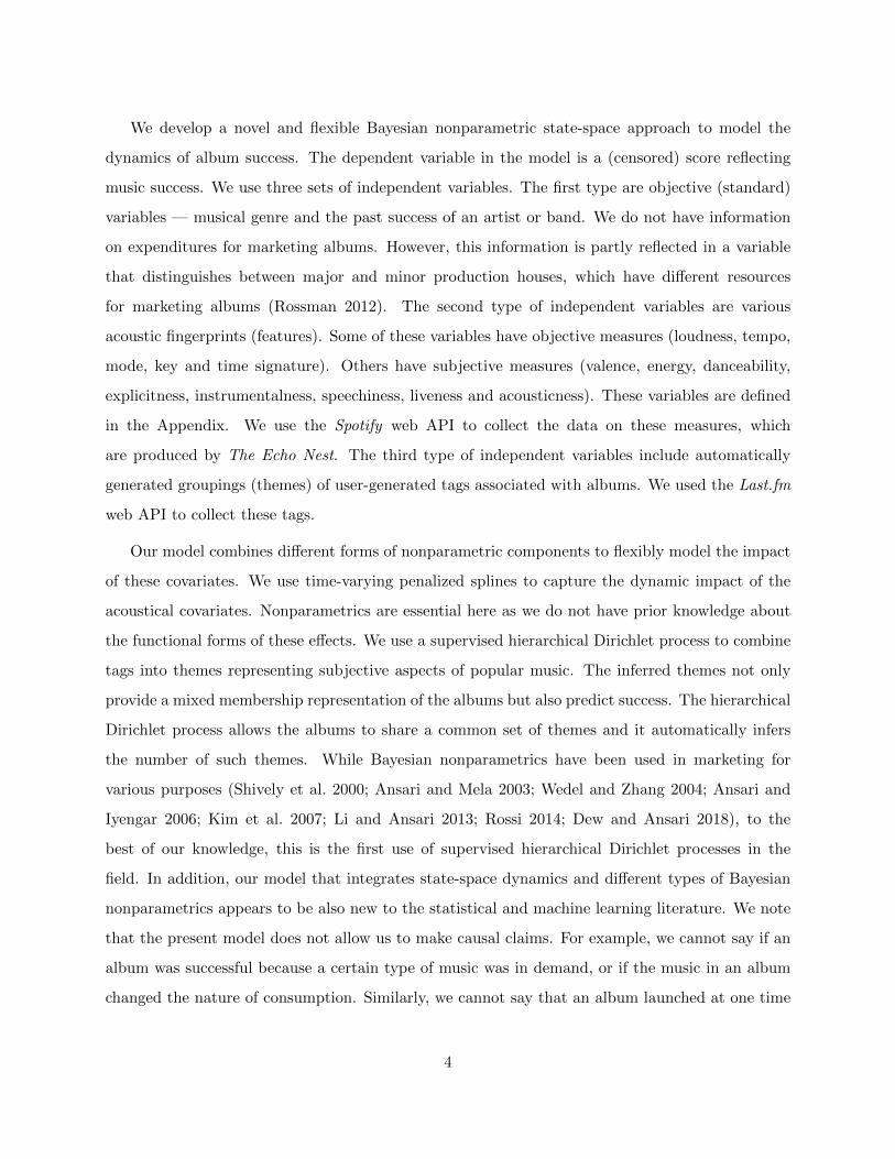
Figure 2 shows a word cloud of all the unique tags in our data. Figure 3 Shows the tags

6For example, if an album has the following weighted tags (Female Singer, 100), (Love, 80) and (Guitar, 20), thenits bag of tags includes 100/(100 + 80 + 20) = 50 replications of the tag “Female Singer”, 80/(100 + 80 + 20) = 40replications of the tag “Love” and 20/(100 + 80 + 20) = 10 replications of the tag “Guitar”.

11

Figure 3: Wordcloud for the Tags of: (left) Thriller (1982) Michael Jackson, (middle) 25 (2015) Adele and(right) 1985 (2014) Taylor Swift.

associated with the albums Thriller, 25 and 1989. Tags displayed with larger fonts have higher

weights. Each album has unique and common tags. For example, the unique tags are “male

vocalists”, “halloween” and “classic” for Thriller ; “british”, “blue”, and “epic” for 25 ; and “love

at first listen”, “electropop” and “synthpop” for 1989. The tags common to the three albums are

“pop” and “albums I own.”

3 Modeling Framework

We now develop a novel Bayesian modeling framework that flexibly and nonparametrically

integrates the different data types (genres, acoustic features, tags and marketing variables) to

explain and predict album success. We index the albums by i = 1, . . . , I, with I being the total

number of albums in the dataset. An album can appear on the charts for multiple years and the

albums differ in the number of years they are represented in our data. Let yij be the success score

of the i-th album in its j-th year within the data, where j ∈ {1, . . . Ji}. Also, let t = 1, . . . T index

calendar time in years. We can then link the observations of an album to their calendar year via a

variable t(ij) such that t(ij) = t, if the jth observation for album i is in calendar year t.

In mathematically specifying our framework, it is easier to distinguish among sets of variables

by how they affect success. We model discrete variables in a linear fashion but allow for flexible

nonlinear effects for the continuous variables, and we incorporate the tags via a rich set of latent

probability distributions, which we call as themes. Specifically, for observation j of album i, we

use 1) xij to represent a K-vector of binary variables. These include the genre dummies and other

discrete variables that specify marketing features, such as major label etc., 2) aij to represent a

12

L-vector of continuous variables, where each component takes a value on a compact interval of

the real line. These continuous variables include the acoustical fingerprints and other variables

that are available on a continuous scale (e.g., the number of previous releases of an artist) and 3)

wi = {win}Nin=1 to label the collection of the Ni tags of the album.

3.1 Censored Success Score

Our measure of album success has a discrete-continuous nature due to the limited number of albums

featured on the charts (a maximum of 200 per week). While different measures of album success

(such as peak rank and week count) are observed for the albums that appear on the charts, success

measures for the less fortunate releases that do not make it to the charts are not observable. We

handle this censorship by assuming that the measure yij is a manifestation of an underlying latent

variable y∗ij (Tobin 1958) that characterizes the true score of the album. This partially latent

score is observable for albums that make it to the charts but is latent for the other albums. The

relationship between the observed and the true score is given by

yij =

{y∗ij , if y∗ij ≥ 0,

0, if y∗ij < 0.(1)

We then model the partially latent variable y∗ij . Our model in its most generic form can be specified

as follows:

y∗ij = Ft(ij) (xij ,aij ,wi) + εij , (2)

where Ft(ij) is a time-varying functional that links the latent success variable with the different

types of the covariates of the album, and εij ∼ N(0, σ2ε) is an idiosyncratic error term that follows

a normal distribution. We now describe the link function in greater detail.

3.2 The Link Function

The link function Ft(ij) flexibly captures the impact of the different types of album features and

latent variables on success via an additive specification

Ft(ij) (xij ,aij ,wi) = x>ijβt(ij) + ft(ij)(aij) + gij(wi), (3)

where βt(ij) is a time-varying coefficient vector that captures the impact of the discrete variables,

ft(ij)(.) is a time-varying unknown multivariate function that capture the effect of the continuous

13

variables and gij(.) is a function that quantifies the thematic information in the tags. We now focus

on each component separately.

3.2.1 Dynamic Linear Effects

The effects of the discrete variables are specified linearly as x>ijβt(ij). We use a state-space

specification to model the temporal changes in the influence of these variables. Specifically, we

assume that the coefficients βt for calendar year, t follow a random-walk,

βt = βt−1 + ωβt , (4)

where the residual vector ωβt is normally distributed, N (0,Σβ), with Σβ = Diag(σ2β1, . . . ,σ2

βJ)

being a diagonal covariance matrix. The variance components σ2βj for j = 1, . . . , J, capture the

volatility of these coefficients over time, with larger values implying greater volatility.

3.2.2 Dynamic Nonparametric Effects

The effects of the continuous covariates (e.g. acoustic fingerprints) are modeled in a dynamic and

nonparametric manner through calendar time specific functions ft(ij)(aij). We use an additive

specification,

ft(ij)(aij) =L∑`=1

h`t(ij)(aij`),

where, h`t(ij)(.) is a smooth function for continuous variable `. We model these unknown functions

using penalized splines (Wand and Ormerod 2008). Such a nonparametric specification allows us

to flexibly specify these effects, as it is not possible to a priori hypothesize how these covariates

influence album success. The use of penalized splines allows us to seamlessly trade-off the flexibility

and smoothness of the inferred functions.

We assume that for a given calendar year t, each component h`t(.) is a piecewise polynomial

function of degree two, represented as

h`t(ait`) = ψ`t0 +ψ`t1ait` +ψ`t2a2it` +

Q∑q=1

ψ`κq(ait` − κ`q)2+, (5)

where, {ψt0,ψ`t = [ψ`tr]2r=1,ψ

`κ = [ψ`κq]

Qq=1} are parameter coefficients to be estimated, and κ`1 <

· · · < κ`Q are fixed knots. In the above, we use quadratic basis splines involving the second-degree

14

truncated basis function

(aij` − κ)2+ = (aij` − κ)2δaij`≥κ, (6)

where, δaij`≥κ = 1, if ait` ≥ κ, and 0, otherwise, and κ is a fixed knot in the compact support of

aij`. Usually a tradeoff exists between using a large number of knots to increase the fidelity to the

data and the smoothness of the resulting function. A roughness penalty is then used to adequately

resolve this trade off. We use a fixed number of knots with known positions but constrain their

influence via the use of Bayesian priors.

Additive Model Summing over all L additive nonlinear effects, the functional ft(.) can be

written as

ft(ait) = ψt0 +L∑`=1

2∑r=1

ψ`trarit` +

Q∑q=1

ψ`κq(ait` − κ`q)2+

, (7)

where ψt0 =∑L

`=1 ψ`t0 is a non-identified intercept, which we fix to zero. Sun et al. (1999) showed

that the above setup in Equation 7 can be represented as a mixed model with additional covariate-

specific hierarchical variance components σ2ψκ` that control the amount of smoothing for the basis

coefficients by assuming that ψ`κq ∼ N (0, σ2ψκ`).

Under this representation, the polynomial coefficients ψ`tr, the basis coefficients ψ`κq, and the

prior variances σ2ψκ are all inferred from the data. In particular, as σ2ψκ is estimated, the implicit

regularization that it induces ensures that only the important knots parameters are given significant

weights. Small values of σ2ψκ diminish the effect of the truncated basis, whereas, larger values allow

the basis coefficients to significantly deviate from zero and thus allow a greater effect of the truncated

basis. Till now we focused on the nonlinear effects for a given calendar year. We now show how

these vary across the years.

Function Dynamics We again use a state-space approach to allow the nonparametric functions

to vary across the calendar years. This ensures that functions for neighboring years are more

similar than for years that are temporally far apart. We specify these function dynamics via the

time-varying polynomial coefficients ψt = {ψ`t1,ψ`t2, ∀`}. Specifically, we assume that ψt follows a

random walk

ψt = ψt−1 + ωψt , (8)

15

where ωψt ∼ N (0,Σψ) with a diagonal covariance matrix Σψ = diag(σ2ψ11, . . . ,σ2

ψL2). Smaller

values of the variances in Σψ imply a smoother temporal evolution of these calendar-time-specific

functions. Having discussed the first two components of Equation 3, we now focus on the last

component that incorporates the perceptual tags.

3.2.3 Nonparametric Themes

Apart from the discrete (e.g. genre) and the continuous variables (e.g. acoustic fingerprints),

album success can also be explained in terms of the tags. Due to their very large number, it is

difficult to account for all the tags directly in the model. Instead, we incorporate their effects via a

thematic categorization of the albums. In inferring these themes, we ensure that we only uncover

those themes that are predictive of album success. We model these themes using a supervised

hierarchical Dirichlet process specification. We begin by describing what we mean by themes.

Themes We define a theme as a discrete probability distribution over the entire vocabulary of

tags. We index each tag in the vocabulary by v ∈ {1, . . . , V }, where V is the total number of

unique tags. A theme is more formally described by φw = [φwv ]Vv=1 with∑V

v=1 φwv = 1. The theme,

therefore, resides in the V − 1 dimensional simplex, where φv refers to the probability with which

tag v appears in the theme. Note that all the tags appear in all the themes but with different

occurrence probabilities (possibly null), which means that the themes are differentiated by the

weights they place on each of the V tags. As the number of themes is unknown a priori, we

consider a nonparametric framework where we assume that there is a countably infinite number of

themes [φwk ]∞k=1 that are shared across all the albums. For each theme φwk , we assign a scalar φyk

that indicates the contribution of the theme to the success of an album. Thus, each “augmented”

theme is fully defined by the tuple φk = (φwk , φyk).

Albums as a Mixture of Themes The collection of tags of an album can be considered as

a mixture of the themes [φk]∞k=1. The albums differ in the weights they place on these themes.

We assume that album i on its jth year draws its themes from an unknown discrete distribution

Gij that is defined over the themes [φk]∞k=1. Let θijn = (θwijn, θ

yijn) denote the augmented theme

associated with the n-th tag, win, of album i on observation j, where θwijn is equal to one of the

16

probability vectors in [φwk ]∞k=1 and θyijn is its corresponding success score. Then,

θijn|Gij ∼ Gij .

The tags within an album probabilistically originate from specific themes. In particular, each

tag win is a random multinomial (categorical) draw, given the chosen theme, i.e.,

win|θwitn ∼ Categorical(θwitn). (9)

Note that the set wi of the Ni tokens within the album can contain many replications of the same

tag from different users, and that two replicates of the same tags can come from different themes.

Finally, the themes relate to overall album success via the component gij(wi) in Equation 3. This

component is given by the average of the success coefficients of the underlying themes for its tags,

gij(wi) =1

Ni

Ni∑n=1

θyijn. (10)

The above shows how the themes differ across albums via the album-specific distributions, and how

the tags as well as album success scores inform the inference of the themes. However, given that

the Gij vary across albums, it is important to ensure that these distributions all share the same

set of themes. This requires that the album-specific distributions are discrete and share the same

atoms. This can be achieved via a supervised hierarchical Dirichlet process (SHDP) specification,

which we now describe.

Supervised Hierarchical Dirichlet Process As the distributions Gij are unknown, we assume

that these come from a Dirichlet process, i.e.,

Gij ∼ DP (α0, G0),

with a baseline distribution G0 and a precision parameter α0 > 0. The Dirichlet process is

a distribution over distributions that is used as a prior in Bayesian nonparametrics to model

uncertainty about the functional form of an unknown distribution. Random draws from the DP

are discrete measures with probability one. The Dirichlet process has been used in marketing

primarily to flexibly represent unobserved heterogeneity via nonparametric population distributions

over coefficients; see Ansari and Iyengar (2006) and Li and Ansari (2013).

17

The fact that a DP generates discrete distributions is by itself not sufficient in our context. It is

also necessary that the album-specific distributions all have support on the same set of themes. This

can be achieved by restricting the baseline distribution G0 to be discrete. Note that if G0 were to

be continuous, then any two distinct distributions drawn from DP (α0, G0) would necessarily have

different atoms. We therefore specify an additional layer of hierarchy by assuming that G0 itself

comes from another Dirichlet process, i.e.,

G0|γ,H ∼ DP(γ,H), (11)

where the baseline distribution, H = Hw × Hy is a joint continuous probability measure on the

themes and their corresponding success coefficients, and γ > 0 is the precision parameter. The

baseline distribution H represents the mean of the process and sets its location, while γ controls the

dispersion of the DP realizations, around H. As realizations of the DP are discrete distributions,

assuming a Dirichlet process prior DP(γ,H) over G0 guarantees a discrete support for G0 such

that it places its mass over a countably infinite collection of probability vectors and their success

coefficients, Φ = [φk]∞k=1. In this way, G0 initializes the infinite collection of themes that will be

shared across the albums.

The clustering properties of the DP depend upon its precision parameter. In the limit, when γ

tends to zero, the realizations of the DP are concentrated on a single point, whereas for large γ the

realizations mimic the baseline distribution H. We infer γ from the data and are therefore able to

automatically determine the number of themes that are relevant in our context. To complete the

hierarchy, we set Hw = Dir(1/V ), a symmetric Dirichlet distribution, over the entire vocabulary

of tags. This is a non-informative prior that does not discriminate among the themes, and Hy =

N(0, 100), a diffuse normal distribution over the success coefficients for the themes.

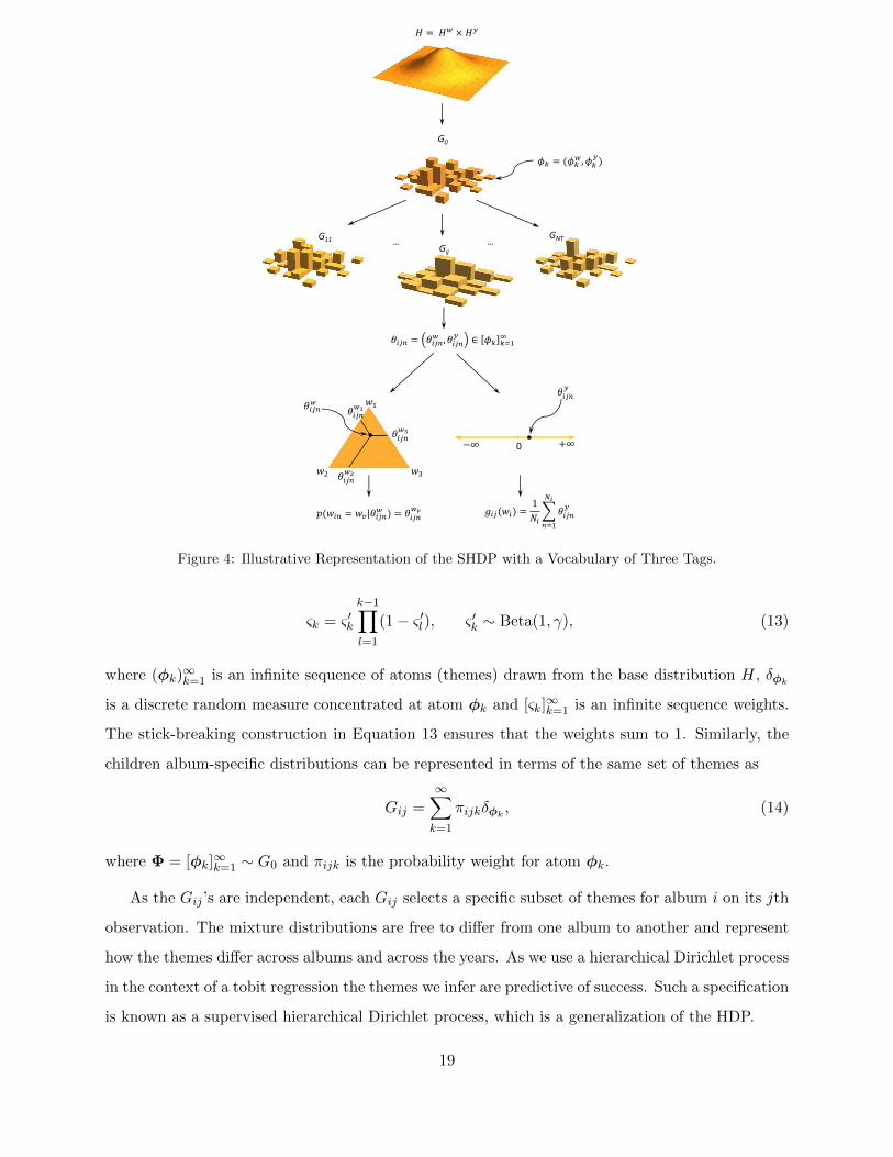
Relationships among the Distributions in the Hierarchy Figure 4 represents the SHDP

with a simplified vocabulary of three tags. Because the mother distribution G0 and the album-

specific distributions that stem from it are discrete, they share the atoms generated from

G0. Sethuraman (1994) showed that a DP can be alternatively construed via a stick-breaking

construction. According to his representation, G0|γ,H ∼ DP(γ,H) can be written as

G0 =∞∑k=1

ςkδφk , φk ∼ H, (12)

18

G11

Gij

GNT

𝜙𝑘 = (𝜙𝑘𝑤 , 𝜙𝑘𝑦)

𝐻 = 𝐻𝑤 × 𝐻𝑦

G0

𝑤1

𝑤2 𝑤3

𝜃𝑖𝑗𝑛𝑤

−∞ +∞

𝜃𝑖𝑗𝑛𝑦

… …

0

𝑝(𝑤𝑖𝑛 = 𝑤𝑣|𝜃𝑖𝑗𝑛𝑤 ) = 𝜃𝑖𝑗𝑛

𝑤𝑣 𝑔𝑖𝑗(𝑤𝑖) =1

𝑁𝑖

𝑛=1

𝑁𝑖

𝜃𝑖𝑗𝑛𝑦

𝜃𝑖𝑗𝑛𝑤1

𝜃𝑖𝑗𝑛𝑤3

𝜃𝑖𝑗𝑛𝑤2

𝜃𝑖𝑗𝑛 = 𝜃𝑖𝑗𝑛𝑤 , 𝜃𝑖𝑗𝑛

𝑦∈ 𝜙𝑘 𝑘=1

∞

Figure 4: Illustrative Representation of the SHDP with a Vocabulary of Three Tags.

ςk = ς ′k

k−1∏l=1

(1− ς ′l), ς ′k ∼ Beta(1, γ), (13)

where (φk)∞k=1 is an infinite sequence of atoms (themes) drawn from the base distribution H, δφk

is a discrete random measure concentrated at atom φk and [ςk]∞k=1 is an infinite sequence weights.

The stick-breaking construction in Equation 13 ensures that the weights sum to 1. Similarly, the

children album-specific distributions can be represented in terms of the same set of themes as

Gij =∞∑k=1

πijkδφk , (14)

where Φ = [φk]∞k=1 ∼ G0 and πijk is the probability weight for atom φk.

As the Gij ’s are independent, each Gij selects a specific subset of themes for album i on its jth

observation. The mixture distributions are free to differ from one album to another and represent

how the themes differ across albums and across the years. As we use a hierarchical Dirichlet process

in the context of a tobit regression the themes we infer are predictive of success. Such a specification

is known as a supervised hierarchical Dirichlet process, which is a generalization of the HDP.

19

3.3 Generative Process

We combine together the success measure, the standard covariates, the linear variables and the tag

applications to jointly uncover the correlates of album success. Given the previous descriptions our

model can be specified using the following generative process.

1. Draw hyper-distribution of themes and their success coefficients, G0 ∼ DP(γ,H)

2. Draw the truncated basis coefficients of the non-linear effects, ψκ ∼ N (0, σ2ψκI)

3. For each year t,

(a) Draw linear effects coefficients, βt ∼ N (βt−1,Σβ)

(b) Draw the linear coefficients of the non-linear effects , ψt ∼ N (ψt−1,Σψ)

4. For each observation j of album i, appearing in year t(ij),

(a) Draw thematic mixture Gij ∼ DP(α0, G0)

(b) For each tag application n,

i. Draw theme θijn = (θwijn,θyijn) ∼ Gij

ii. Draw tag win ∼ Categorical(θwijn)

(c) Draw score yij ∼ N (Ft(xit,ait(ij),wi

), σε)

3.4 Posterior Inference via MCMC methods

We use a fully Bayesian approach to infer the unknowns in our model specification. Let Γ =

{y∗ij},β0:T ,Σβ,ψ0:T ,Σψ,ψκ, σ2ψκ, {θijn}, α0, γ, σ

2ε} contain all the random variables to be estimated.

Then the joint distribution of the data and unknowns can be written as

p({yij},{y∗ij},w1:I ,Γ) =I∏i=1

∏j∈Ti

p(yij |y∗ij)p(y∗ij |βtij ,ψtij ,ψκ,wi, {θijn})

×T∏t=1

p(βt|βt−1,Σβ)p(ψt|βt−1,Σψ)p(ψκ|σ2ψκ)×I∏i=1

∏i∈Ti

Ni∏n=1

p(win|θijn)p(θijn|α0, γ)

×p(σ2ε)p(β0)p(ψ0)p(Σβ)p(Σψ)p(σ2ψκ). (15)

Note that we integrate over the mixture distributions Gij and G0 and perform direct inference on

the albums themes θijn. As the full posterior distribution p(Γ|{yij},wi) does not have a closed

form formulation we use MCMC methods to summarize the posterior. We use conjugate priors

20

and therefore all the full conditional distributions are available analytically. We use backward-

filtering forward-smoothing to sample the dynamic linear coefficients and the parameters of the

linear component of the penalized splines. The integration of the HDP priors specifically leads to

a collapsed Gibbs sampling scheme for the inference regarding the themes. We use the algorithm

based on direct assignment of the tags that is described in more details by Teh et al. (2005).

The inference algorithm was implemented in Python. Our big data context requires efficient

computation; hence, we use numba to compile the code to processor language. More details about

the full conditionals can be obtained upon request, and the code itself is available from the first

author’s website.

4 Results

We first compare the preceding model with a set of benchmark models on a number of predictive

metrics. Then we highlight the qualitative insights obtained from the model.

4.1 Model estimation and comparison

We estimated three benchmark models. Model M1 used artist superstardom, major label, number

of previous years on the charts and number of artists on the album as predictor variables. Model M2

added album genre to the variables in M1; and model M3 added acoustic features to the variables

in M2. We label the proposed model M4; it includes the variables in M3 and the user generated

tags. We introduced time dynamics in each model via state-space specifications and nonparametric

functional forms for the continuous covariates.

We estimated each model using MCMC methods. The Markov chains converged with 4,000

iterations for models M1, M2 and M3. We report their results using the last 2,000 MCMC draws

after burn-in. Model M4, which includes textual data, required more iterations. We ran the

chain for 50,000 iterations and retained the last 5,000 iterations after burn-in. We normalized all

continuous variables (e.g., acoustic features) to a scale between zero and one to allow meaningful

comparisons across variables. We log-transformed the year end score so as to stabilize numerical

computations.

We split the dataset into calibration and holdout samples, the latter containing a random

21

Table 2: Measures of Predictive Performance.

Sample Metric M1 M2 M3 M4

Calibration

AUC 0.61 0.71 0.80 0.82RMSE 6.85 6.10 5.39 5.21Correlation 0.25 0.37 0.50 0.52Predictive R2 0.06 0.13 0.23 0.25

Holdout

AUC 0.59 0.68 0.76 0.77RMSE 6.91 6.64 6.26 6.07Correlation 0.22 0.30 0.40 0.44Predictive R2 0.04 0.07 0.13 0.15

sample of 10% albums available for each year. The calibration sample has 23,036 observations and

the holdout sample has 2,535 observations. We re-estimated all models on the calibration data and

used the estimated parameters to make the holdout predictions. These predictions were made using

a semi-supervised approach: the holdout albums were used in model calibration but without their

success scores. This allowed the use of tags for the validation albums to be used for estimating the

themes.

Predictive performance We assessed the predictive performance of the models in terms of (1)

the probability of an album appearing on the charts and (2) the album rank, conditional on it

making the charts. To assess how well the predicted probability tracks the actual probability of

making the charts, we used the Area Under the Curve (AUC) of a model’s Receiver Operating

Characteristic (ROC) curve (Swets, 1996). The best-performing model has the highest AUC. We

validated the prediction of album rank by using the root mean square error (RMSE) and the

correlation of the observed and estimated success scores for an album. Table 2 reports the values

of these predictive measures for in-sample and holdout data. For both in-sample and out-of-sample

data, the full model, M4, predicts the probability of making the charts and the rank on the charts

better than the competing models. The total explained variance can be decomposed between the

different sets of covariates. Based on the predictive R2 values, genre explain about 28% of the total

variance, acoustic fingerprints 40%, tags 10% and the marketing and superstardom variables about

22%.

22

4.2 Qualitative Insights

We divide the discussion of the results into four sections. First, we discuss how the popularity

of different genres has fluctuated and changed over time. Second, we examine how the level and

variability in acoustic features affects its success. Third, we examine how the perceptual and

experiential aspects of music, reflected in the crowd-sourced tags, affect album success. Fourth, we

discuss the temporal effects of the marketing and superstardom variables on album success.

4.2.1 The Dynamics of Genre Popularity

The figure in Table 3 shows how the appeal of different genres has changed over time. The vertical

axis in each of the plots indicates the estimate predictor of success for each genre.

Rock: Rock music is the most produced genre in our dataset. The “British invasion” of American

popular music coincides with the peak of rock music in the 60s. Classic albums of the period include

the following by the Beatles: Sgt. Pepper’s Lonely Hearts Club Band, Revolver and The Beatles.

Albums like Pink Floyd’s The Dark Side of the Moon drove Rock music to another peak in the 70s.

Since then, the popularity of Rock music has declined while Pop and Hip Hop have risen; and Rock

music itself has fragmented into specialized forms. The recent resurgence since 2010s has been led

by albums like Blurryface by Twenty One Pilots.

Pop: Pop music has had significant periods of popularity. The 60s peak saw the release of More

of the Monkeys by the Monkeys and Herb Alpert’s Whipped Cream & Other Delights. New styles

of Pop emerged in the 80s, the most notable being Michael Jackson’s Thriller and Prince’s 1999.

Recently, Pop has again shown a positive trend in popularity with the launch of albums like Taylor

Swift’s 1989, Adele’s 21, and Ed Sheeran’s x.

Funk & Soul: Funk & Soul music has had two previous peaks. The first, in the 70s, coincided with

the release of albums like I Never Loved A Man The Way I Love You by Aretha Franklin. The

second, in the 80s, coincided with the releases of Prince’s Purple Rain and Wham!’s Make It Big.

The genre has witnessed an increase in popularity since the 90s, with the release of albums like 25

by Adele and TRAPSOUL by Bryson Tiler.

23

Tab

le3:

Patt

ern

sof

Gen

res

Pop

ula

rity

acr

oss

Tim

e.

Pea

kAlbum

Name

Pea

kAlbum

Name

TheDark

Sideofth

eMoon,PinkFloyd(1973)

Crazy

sexyco

ol,TLC

(1995)

1Summer

Breeze,

Sea

lsandCrofts(1973)

9II,BoyzII

Men

(1995)

Don’t

ShootMeI’m

Only

ThePianoPlayer,EltonJohn(1973)

Brandy,

Brandy(1995)

Blurryface,Twen

tyOnePilots

(2016)

LoveAngel

MusicBaby,

Gwen

Stefani(2005)

2Montevallo,Sam

Hunt(2016)

10

Goodies,

Ciara

(2005)

Immortalized,Distu

rbed

(2016)

TheMassacre,

50Cen

t(2005)

More

OfTheMonkees,TheMonkees(1967)

TheVeryBestofPeter,PaulandMary,Peter,PaulandMary

(1964)

3W

hipped

Cream

&Oth

erDelights,HerbAlpert&

TheTijuanaBrass

(1967)

11

Today,

TheNew

ChristyMinstrels

(1964)

WhatNow

MyLove,

HerbAlpert&

TheTijuanaBrass

(1967)

JoanBaez,JoanBaez

(1964)

Thriller,Michael

Jack

son(1983)

August

AndEveryth

ingAfter,CountingCrows(1994)

41999,Prince

(1983)

12

NotA

Momen

tTooSoon,Tim

McG

raw

(1994)

KissingToBeClever,Culture

Club(1983)

Reb

aMcE

ntire’s

Greatest

Hits,

VolumeTwo,Reb

aMcE

ntire

(1994)

1989,TaylorSwift(2015)

BeHere,

Keith

Urb

an(2005)

5x,EdSheeran(2015)

13

HereForTheParty,

Gretchen

Wilson(2005)

Montevallo,Sam

Hunt(2015)

TobyKeith

35BiggestHits,

TobyKeith

(2005)

INev

erLoved

AManTheW

ayILoveYou,Areth

aFranklin(1967)

Honey

InTheHorn

,AlHirt(1964)

6HereW

hereThereIs

Love,

DionneW

arw

ick(1967)

14

TheThirdAlbum,Barb

raStreisand(1964)

LouRawls

LiveAtTheCen

tury

Plaza

,LouRawls

(1967)

ThePinkPanth

er(O

riginalMotionPictu

reSoun...,Hen

ryMancini(1964)

MakeIt

Big,W

ham!(1985)

What’sNew

,LindaRonstadt(1984)

7BreakOut,

ThePointerSisters

(1985)

15

BodyAndSoul,JoeJack

son(1984)

Purp

leRain,Prince

(1985)

Back

street,David

Sanborn

(1984)

25,Adele(2016)

ComeAwayW

ithMe,

NorahJones

(2004)

8T

RA

PSO

UL,BrysonTiller(2016)

16

Feels

LikeHome,

NorahJones

(2004)

Bea

uty

Beh

indTheMadness,

TheW

eeknd(2016)

ThreeDaysGrace

(DeluxeVersion),

ThreeDaysGrace

(2004)

24

Hip Hop: Hip Hop music is an American form of music that was developed in the 70s. It includes

rhythmic melodies often accompanied with rapping. Hip Hop’s popularity peaked in the 90s with

the release of albums like Crazysexycool by TLC and II by Boys II Men’s. It has maintained its

popularity, with albums like The Massacre by 50 Cent receiving great success.

Folk, Country & World: The 1960s was a golden era for Folk and Country music. Hit albums

included The Very Best of Peter, Paul and Mary and The Freewheelin’ Bob Dylan. The rise of

American folk-music contributed to the development of Country, Jazz, and Rock’n’Roll. The appeal

of Folk and Country music diminished during the 70s and 80s. It made a comeback in the 90s with

modern folk and country styles introduced in the albums The Woman In Me by Shania Twain,

Rumor Has It and For My Broken Heart by Reba McEntire, and Not A Moment Too Soon by

Tim McGraw. The peak in the 2000s saw the emergence of new styles of Country and Folk music,

with albums like Whoa, Nelly! by Nelly Furtado, Be Here by Keith Urban, and Fearless by Taylor

Swift.

Jazz: Jazz has waxed and waned over the years. A peak in the 60s saw successful albums like Honey

in The Horn by Al Hirt and The Third Album by Barbra Streisand. Jazz regained popularity in

the 80s when Linda Rondstadt introduced What’s New. The most recent peak occurred in the

2000s, when Come Away With Me and Feels Like Home were released by Norah Jones.

It is interesting to see how these genres coevolved over the decades. Figure 5 shows the

correlation in the time-varying coefficients βt of the genre dummies for different pairs of genres.

It is clear from the figure that certain genres behaved like substitutes, as can be seen from the

negative correlation between Rock and Hip Hop, or Pop and Electronic. Other genre pairs exhibit

positive correlations, as they grew or declined together, as for example, Funk and Soul and Pop,

or Reggae and Hip Hop.

4.2.2 Acoustic Features and Album Success

We examine how the success of an album is related to the average levels of the acoustic features

and their variances across the songs in an album. As noted, we distinguish between “objective”

and “subjective” acoustic features. Objective features refer to technical characteristics of the music

itself and subjective features pertain to the experiential aspects of music. Recall that album-level

acoustic measures have a nonlinear relation with album success within any given year, and the

25

Figure 5: Correlations of the Time-Varying Genre Coefficients.

pattern of nonlinearity can vary across the years. Figures 6 and 7 show the dynamics of these

nonlinear effects for both the average acoustic levels and their standard deviations

Objective Features

Loudness: Loudness, the physical strength of the sound in an album, is positively associated with

success over the years. The appeal of loud music peaked during the 80s and 90s and has recently

diminished slightly. Serra et al. (2012) found that popular songs have been getting louder over the

years. A significant effect of the standard deviation of loudness suggests that mixing louder and

softer songs adds to an album’s appeal as a uniformly loud album can irritate a listener.

Tempo: Tempo characterizes the speed of the music. Albums with slow tracks on average were

more successful in most years. The exceptions were the early 1960s (rock’n’roll days), early 1980s

(emergence of new rock genres like punk and heavy metal) and the recent 2000s. Since the 2000s,

26

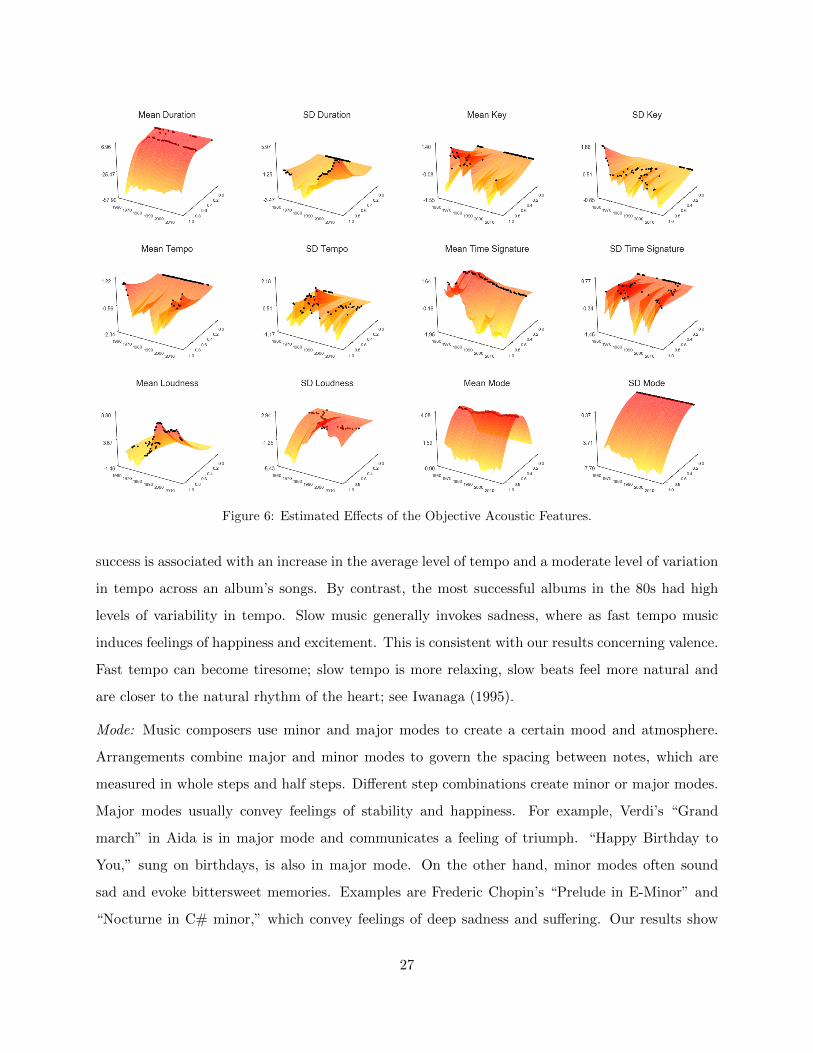
Figure 6: Estimated Effects of the Objective Acoustic Features.

success is associated with an increase in the average level of tempo and a moderate level of variation

in tempo across an album’s songs. By contrast, the most successful albums in the 80s had high

levels of variability in tempo. Slow music generally invokes sadness, where as fast tempo music

induces feelings of happiness and excitement. This is consistent with our results concerning valence.

Fast tempo can become tiresome; slow tempo is more relaxing, slow beats feel more natural and

are closer to the natural rhythm of the heart; see Iwanaga (1995).

Mode: Music composers use minor and major modes to create a certain mood and atmosphere.

Arrangements combine major and minor modes to govern the spacing between notes, which are

measured in whole steps and half steps. Different step combinations create minor or major modes.

Major modes usually convey feelings of stability and happiness. For example, Verdi’s “Grand

march” in Aida is in major mode and communicates a feeling of triumph. “Happy Birthday to

You,” sung on birthdays, is also in major mode. On the other hand, minor modes often sound

sad and evoke bittersweet memories. Examples are Frederic Chopin’s “Prelude in E-Minor” and

“Nocturne in C# minor,” which convey feelings of deep sadness and suffering. Our results show

27

that across the years, successful albums typically combine these two modes in equal proportions

(an average mode around 0.5 and a small variance of modes).

Keys: The major and minor modes are associated with 12 basic notes represented by an integer from

0 to 11 with the note C=0, C]=1, and so on until we reach B = 11. These combinations are called

keys; they map a song to its corresponding pitch and allow us to judge a song as “high” or “low.”

Some keys are more convenient than others for composing music on certain instruments, allowing

more freedom for the melody to evolve. Low keys (mainly E, C and G) are more convenient for

composition on a piano or a guitar. Our results show that, except in the 1970s and 1980s, successful

albums had low keys. Variability of the keys across album tracks is appealing for most of the years

in our dataset. However, this appears to have flipped in the last few years where successful albums

have songs in low keys and low variance in the keys.

Time signature: Time signature characterizes the number of beats in a bar. The common time

signatures in Western music are: 4/4, 3/4, 2/4 and 6/8. A listener experiences the time signature

in a song’s rhythm. The most common time signature is 4/4. Some musical styles, mainly jazz,

experiment with other odd rhythms. Our results show that successful albums have a dominant low

average time signature over time. The exception is popular music in the 1960s and 1970s, which

inherited aspects of 50s jazz music. Successful albums across the years exhibit different variations

of time signatures. In the 1970s, 1990s and the 2010s, albums with high variation in time signatures

were more successful; in the 1960s, 1980s and 2000s, albums with lower variation in time signature

variance were more appealing.

Subjective Features

Valence: Focusing on Figure 7, the subplots associated with valence show that albums with an

average negative valence (i.e., sad or angry) have been more successful on the charts. Our results

also indicate that an emotional balance within the album is preferred to having only happy or sad

songs. This is consistent with Koelsch et al. (2006) who found that although sad music necessarily

evokes sadness, it is also more enjoyable as it activates other positive emotions and has a greater

aesthetic appeal (Scherer 2004; Zentner et al. 2008).

Acousticness: Recall that acousticness predicts the extent to which a song contains natural sounds

(e.g., guitar or harmonica) as opposed to the addition of electronic (i.e., computer derived) sounds.

28

Figure 7: Estimated Effects of the Subjective Acoustic Features.

We see that successful albums became less acoustic over the years, as with the advent of synthesizers,

new technologically innovated sounds were incorporated in music production (Starr and Waterman

2018). We also see that in the recent years albums that contain high variability of acoustic and

non-acoustic songs have tended to be more successful.

Energy: The energy measure indicates the experienced strength of a song. For example, a smooth

jazz song has less “energy” than a rock metal track. Our results indicate an interesting pattern.

We see that albums with high average energy were more successful before 1980 and that this trend

has gradually reversed since then. The early success in the 60s can be explained by the popularity

of energetic genres such as rock and dance-oriented music. The peak in the 70s stemmed from the

29

popularity of disco and rock, with the rise of Led Zeppelin and Stevie Wonder. We also see that

the effect for the standard deviation mirrors that of the average level.

Danceability: One of the most important features of music is that it invokes the willingness to

dance. Our results indicate that danceable albums have been more successful across all the years.

There were peaks before 1990s when the market demanded danceable songs due to the expansion

of dance clubs. This trend started with the twist craze of the late 1960s and the disco craze of the

1970s. Again, we see that success is associated with a balance between highly danceable and less

dance focused songs within an album.

Explicitness: Albums with an appropriate level of explicitness are more appealing than the albums

with no explicit songs or exclusively explicit songs. This effect is consistent through the decades.

Albums with high variation in their explicitness are less popular than those with low variability.

Instrumentalness: Albums that have low instrumentalness, i.e., albums that contain vocals, are

more successful than albums that contain instrumental only tracks. High levels of diversity in

instrumentalness is more successful except very recently when lower levels of variability on this

feature appears to be more popular.

Speechiness: Words in music can convey emotions, tell stories and give messages. Albums

containing many lyrical songs or poetry have been more successful since the 1960s. This effect

peaked in the 1990s with the emergence of rap music. The effect of speechiness on album success

has since diminished but we still prefer albums with songs that have spoken words. High variability

in the speechiness of songs characterized successful albums in the 1960s and 1970. This effect, too,

has since diminished. Since the 2000s we prefer album with an “ideal” level of variability in

speechiness.

Liveness: Live recordings convey the energy and the experience lived during a concert or a live

performance of an artist or a band. Albums containing many songs that are recorded live were

more successful in the years of rock bands, particularly the 1960s and 1970s. This trend reversed;

since the 80s, albums featuring live recordings have been less successful.

30

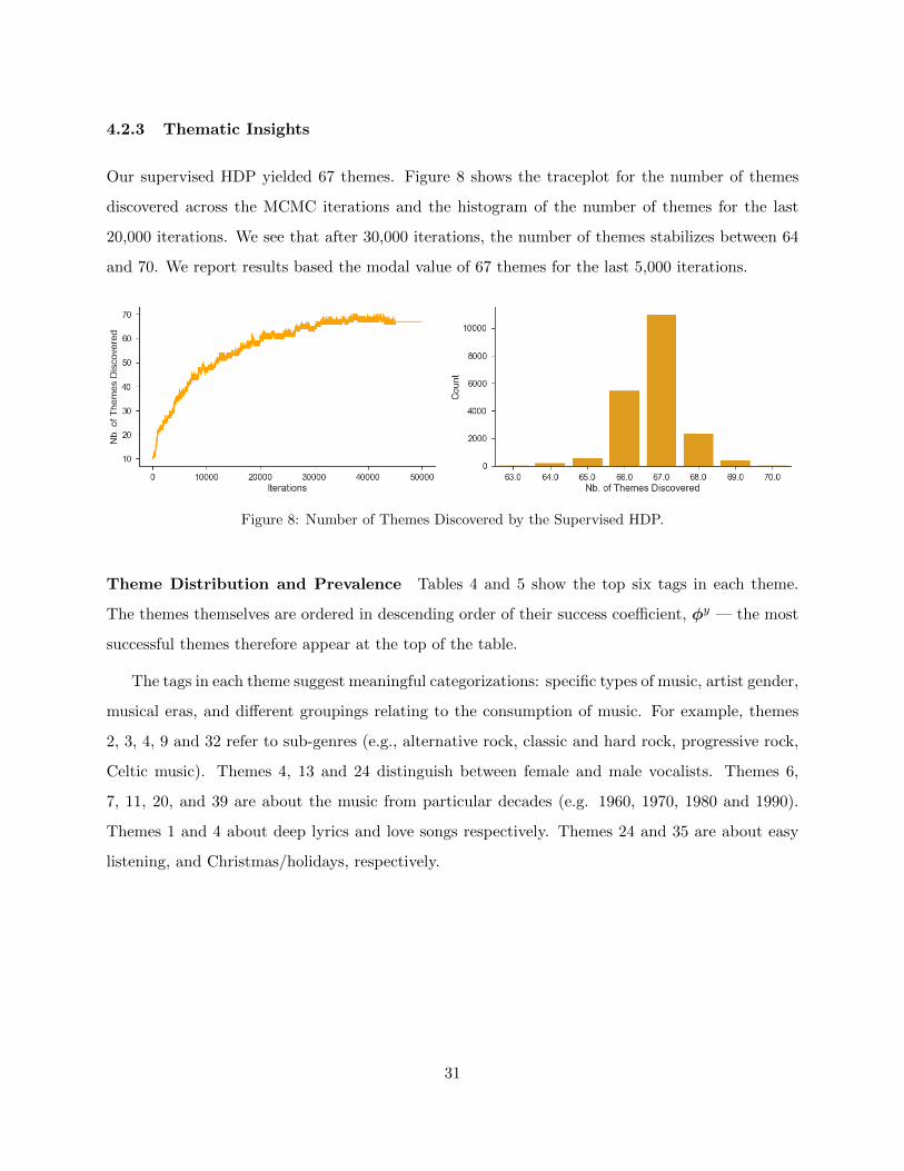
4.2.3 Thematic Insights

Our supervised HDP yielded 67 themes. Figure 8 shows the traceplot for the number of themes

discovered across the MCMC iterations and the histogram of the number of themes for the last

20,000 iterations. We see that after 30,000 iterations, the number of themes stabilizes between 64

and 70. We report results based the modal value of 67 themes for the last 5,000 iterations.

Figure 8: Number of Themes Discovered by the Supervised HDP.

Theme Distribution and Prevalence Tables 4 and 5 show the top six tags in each theme.

The themes themselves are ordered in descending order of their success coefficient, φy — the most

successful themes therefore appear at the top of the table.

The tags in each theme suggest meaningful categorizations: specific types of music, artist gender,

musical eras, and different groupings relating to the consumption of music. For example, themes

2, 3, 4, 9 and 32 refer to sub-genres (e.g., alternative rock, classic and hard rock, progressive rock,

Celtic music). Themes 4, 13 and 24 distinguish between female and male vocalists. Themes 6,

7, 11, 20, and 39 are about the music from particular decades (e.g. 1960, 1970, 1980 and 1990).

Themes 1 and 4 about deep lyrics and love songs respectively. Themes 24 and 35 are about easy

listening, and Christmas/holidays, respectively.

31

Tab

le4:

Top

Six

Tags

Ass

oci

ate

dw

ith

Th

emes

1to

33.

Th

eme

Top

6T

ags

1ro

ber

titu

sgl

obal

,fu

nkyra

m,

legi

t,d

eep

lyri

cs,

1990

s,am

bie

nt

ram

2al

bu

ms

iow

n,

rock

,al

tern

ativ

ero

ck,

alte

rnat

ive,

favo

rite

alb

um

s,fa

vou

rite

alb

um

s3

cou

ntr

y,cl

assi

cco

untr

y,m

od

ern

cou

ntr

y,co

untr

yp

op,

outl

awco

untr

y,av

aila

ble

on

emu

sic

4p

op,

fem

ale

voca

list

s,p

opro

ck,

dan

ce,

fem

ale

voca

list

,lo

veso

ngs

5in

stru

men

tal,

pia

no,

new

age,

celt

ic,

iris

h,

win

dh

amh

ill

reco

rds

620

12,

2011

,20

10,

ind

ie,

ind

iero

ck,

10s

7al

bu

ms

iow

n,

00s,

ind

ie,

2008

,20

07,

ind

iero

ck8

cros

sfad

e,al

bu

ms

ih

ave

dow

nlo

aded

,ei

ghth

grad

ero

cked

,re

lax,

dis

cove

rock

ult

,b

est

alb

um

s9

rock

,cl

assi

cro

ck,

har

dro

ck,

vin

yl

iow

n,

soft

-rock

,al

bu

mro

ck10

cou

ntr

yro

ck,

awes

ome,

favo

rite

,m

mfw

cl,

goth

ic,

goth

icro

ck11

90s,

gru

nge

,19

93,

1990

,19

94,

1996

12so

un

dci

ty,

hav

eth

is,

f,m

isc,

1,80

’s13

fem

ale

voca

ls,

won

der

ful

wom

en,

iow

n,

wie

alle

sb

egan

n,

ben

atar

,fe

mal

evo

cal

14ra

p,

hip

-hop

,h

iphop

,ga

ngs

tara

p,

wes

tco

ast

rap

,ea

stco

ast

rap

15h

ard

rock

,h

eavy

met

al,

met

al,

alte

rnat

ive

met

al,

thra

shm

etal

,nu

met

al16

amer

ican

idol

,al

bu

ms

of20

10,

alb

um

siow

n,

pu

rch

ased

2011

,p

urc

has

ed20

10,

love

at

firs

tli

sten

17so

ul,

rnb

,fu

nk,

r&b

,m

otow

n,

neo

-sou

l18

vin

yl,

lati

n,

own

onvin

yl,

cd,

lati

np

op,

regg

aeto

n19

my

alb

um

s,b

each

mu

sic,

seen

live

,vic

kie

mar

ieh

all,

ken

ny

ches

ney

,b

oyb

and

s20

70s,

1001

alb

um

syo

um

ust

hea

rb

efor

eyou

die

,d

isco

,19

73,

1971

,19

7521

2013

,fo

lk,

sin

ger-

songw

rite

r,fo

lkro

ck,

acou

stic

,am

eric

ana

22ja

m,

vir

alb

rain

dea

th,

wb

reco

rdin

g,gr

eate

sth

its,

jam

ban

d,

cdi

own

23al

bu

ms

inm

yco

llec

tion

,al

bu

ms

iw

ant,

alb

um

si

wor

ked

on,

step

han

iem

ills

,r

an

db,

live

wir

e24

easy

list

enin

g,so

un

dtr

ack,

clas

sica

l,voca

l,m

ale

voca

list

,op

era

25la

pto

p,

ih

ave

this

alb

um

,u

sa,

mal

esi

nge

rso

ngw

rite

r,so

ftro

ck,

amer

ican

mu

sici

an

2680

s,n

eww

ave,

1982

,gr

amm

ynom

inat

ed,

pos

t-p

un

k,

1983

2720

14,

2015

,p

ost-

har

dco

re,

met

alco

re,

har

dco

re,

kil

lfor

pea

ce28

top

cd,

my

favo

rite

s,le

apsa

nd

80sa

lbu

ms,

elec

tric

guit

ar,

gram

use

lsfa

vou

rite

s,m

ein

ealb

en29

chri

stia

n,

chri

stia

nro

ck,

gosp

el,

conte

mp

orar

ych

rist

ian

,w

orsh

ip,

pra

ise

30co

med

y,w

eall

geto

ld,

bet

tem

idle

r,sp

oken

wor

d,

sym

pat

hy68

,st

and

-up

31fu

nk,

2009

,li

ve,

pop

pu

nk,

pu

nk

rock

,p

un

k32

pro

gres

sive

rock

,p

rogr

essi

vem

etal

,ex

per

imen

tal,

pro

gres

sive

,lo

ve,

art

rock

33re

ggae

,fa

vor

ites

,sk

a,co

vers

,co

ver,

1970

32

Tab

le5:

Top

Six

Tags

Ass

oci

ate

dw

ith

Th

emes

34

to67.

Th

eme

Top

6T

ags

34p

arto

n,

bes

tcd

,m

ich

ael

bol

ton

,ad

ult

conte

mp

orar

y,ra

p-a

-lot

reco

rds,

alb

um

si

own

on

cd35

chri

stm

as,

2016

,co

untr

ych

rist

mas

,h

olid

ay,

xm

as,

chri

stm

asm

usi

c36

elec

tron

ic,

dan

ce,

elec

tron

ica,

ind

ust

rial

,sy

nth

pop

,h

ouse

37b

lues

,b

lues

rock

,so

uth

ern

rock

,gu

itar

,ro

ckn

roll

,gu

itar

vir

tuos

o38

jazz

,sm

oot

hja

zz,

flas

hb

ack

alte

rnat

ives

,sa

xop

hon

e,sw

ing,

jazz

voca

l39

60s,

old

ies,

1969

,m

ale

voca

list

s,19

67,

1968

40m

emp

his

rap

,b

ern

stei

n,

albu

ms

iow

np

hysi

call

y,p

arty

,m

aria

chi,

dee

41ca

nad

ian

,d

uet

s,si

nge

r-so

ngw

rite

r,ca

nad

a,w

ood

stock

gen

erat

ion

,b

alla

ds

42kid

s,t

tuck

er,

chil

dre

n,

ysa

bol

sca

rtoon

skid

stv

and

kid

s,am

azin

g,b

aby

43e

har

ris,

bra

ssb

alls

,d

eser

tis

lan

dd

iscs

,fa

vor

ite

alb

um

,n

ew,

bes

tal

bu

ms

ever

4420

04,

grea

tal

bu

ms,

aust

rali

an,

nos

talg

ic,

tw

yn

ette

,u

sher

45ja

zz,

jazz

fusi

on,

fusi

on,

fun

k,

jazz

-fu

nk,

inst

rum

enta

l46

deu

tzia

,n

eed

toge

t,fu

nk

folk

,h

ip-h

opso

ul,

pos

t-b

lack

met

al,

own

onca

sset

te47

1979

,m

yw

hol

ed

amn

coll

ecti

on,

1980

,su

nd

aym

ix,

deb

ut,

full

yst

ream

able

alb

um

s48

1986

stu

dio

alb

um

,la

pis

lazu

li,

ener

geti

c,ja

gged

edge

,b

riti

shfo

lk,

rad

iora

dio

rad

io49

jaso

nm

ich

ael

carr

oll,

the

asto

rs,

pop

pu

nk,

albu

ms

ilo

ved

,fi

refl

ight,

chil

dh

ood

favou

rite

50gl

amro

ck,

psy

ched

elic

,ga

rage

rock

,p

ower

pop

,p

sych

edel

icro

ck,

pow

erp

op51

ind

ie-r

ock

,d

avid

lind

ley,

slid

egu

itar

,ro

oms

and

bu

ild

ings

,b

low

the

roof

,p

salm

150

52re

gin

e-d

isc,

glen

cam

pb

ell,

eigh

ties

,m

otow

nta

g,su

mm

er,

awso

me

guit

ar53

pos

tp

un

k,

ngr

iffith

,n

anci

-gri

ffith

,u

nsu

ng

and

sop

hom

orel

ess,

rock

and

roll

par

ty,

jon

ny

lan

g54

mar

coan

ton

ioso

lis,

met

alic

a,m

oja

do,

troz

osd

em

ial

ma,

blu

eey

edso

ul,

alte

rnai

ve55

un

clas

sifi

able

,ro

cken

esp

ano,

shock

valu

eii

,ca

pri

corn

reco

rds,

md

na,

terr

ible

alb

um

cove

r56

rke

lly,

mr

kell

y,r.

kell

y,ro

ryga

llag

her

,b

lack

ston

e55,

toch

eck

out

57la

tin

jazz

,b

ossa

nov

a,d

ay,

bra

zili

an,

jfu

zz,

bas

s58

big

ban

d,

caly

pso

,cr

oon

er,

swin

g,vo

cal

jazz

grea

ts,

gram

my,

bes

tfe

mal

ep

opvo

cal

per

form

an

cen

om

inee

59on

cein

my

coll

ecti

onof

dat

a,em

i,p

aust

in,

rock

-sym

ph

onie

s,ch

ris

dav

e,dig

it60

mik

ih

owar

d,

ten

oxsa

xra

dio

mix

,al

exb

ugn

on,

smoot

hso

ul,

–get

–,fa

vor

ite

com

edy

alb

um

s61

tom

wai

ts,

dar

kca

bar

et,

tom

jon

es,

colu

mb

ia,

cree

py,

tom

62u

ltra

mag

net

ic,

bro

nx,

boom

bap

,fu

nny,

gold

enag

e,al

tern

ativ

e-co

untr

y63

con

nie

smit

h,

csm

ith

,b

lak,

5ti

mes

orle

ss,

favo

rite

alb

um

s20

05,

sass

jord

an64

my

gan

g11

,li

onel

rich

ie,

pla

yli

st,

lib

pla

yed

,p

opm

usi

cta

g,kic

kass

65ri

char

dth

omp

son

,ch

arli

eh

all,

meg

abu

y30

-10-

17,

the

alb

um

si

list

ened

toso

man

yti

mes

66tw

o-to

ne,

bes

tb

uff

ett,

fbts

um

mer

,le

ave

the

ligh

ton

,h

ayst

ak,

lon

don

67h

er,

arro

nti

pp

in,

mem

orab

le,

alb

um

sth

ati

own

,al

lti

me

bes

t,li

veal

bu

ms

33

Figure 9: Theme Proportions per Decade.

Figure 9 shows the prevalence of these themes across the decades. It shows the average theme

proportion of all the albums within each decade. A darker cell means that the corresponding theme

had a higher proportion in the decade. Themes in Tables 4 and 5 that are specialized in particular

decades have a higher density in the corresponding row in Figure 9. For example, Theme 39 which

has “60s”, “1967”, “1968” and “1969” as the top tags in Table 5 peaks exactly during the 1960s.

This is true for each of the decade related themes, e.g., Theme 6 (2010s), Theme 7 (2000s), Theme

11 (1990s), Theme 26 (1980s) and Theme 20 (1970s).

Themes corresponding to different styles and listening experiences in Tables 4 and 5 also appear

in the relevant years in Figure 9. For example, Theme 2 (rock and alternative rock) was more

prevalent in the 1990s and 2000s. Theme 9 (classic rock, hard rock and soft rock) appears more

in albums of 1970s and 1980s. This was driven by the British invasion (Beatles, Rolling Stone) of

American pop music in the 60s; hard rock became mainstream with the success of bands like Iron

Maiden, Saxon, and Def Leppard. Theme 38 (jazz, smooth jazz and swing) appears more in the

albums of the 1960s; this is consistent with the success of vocal jazz and swing bands in the 50s.

Top Albums Associated with a Theme We can use the vector of themes proportions to

identify the top albums associated with each theme. Tables 6 and 7 show the top two albums that

have the largest proportions associated with each theme. We can identify the meaning of these

themes and how they relate to the different albums by combining the Tables 4, 5, 6 and 7. For

example, the top albums for Theme 4, which is related to female vocalist and live songs, are Kiki

Dee by Kiki Dee and Drinking Again by Dinah Washington. The top two albums of Theme 14,

which is related to rap music, are Encore by Eminem and Lunitik Muzik by Luniz.

34

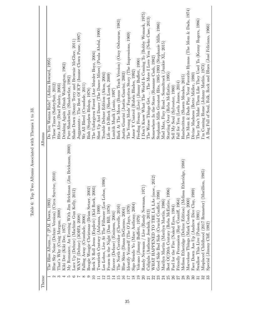
Tab

le6:

Top

Tw

oA

lbu

ms

Ass

oci

ate

dw

ith

Th

emes

1to

33.

Th

eme

Alb

um

s

1T

he

Bli

ssA

lbu

m..

.?(P

.M.

Daw

n,

1993)

Do

You

Wan

na

Rid

e?(A

din

aH

oward

,1995)

2B

lue

Sky

Noi

se(D

elu

xe

Ver

sion

)(C

irca

Su

rviv

e,2010)

Th

ese

Tim

es(S

afe

tyS

uit

,201

2)

3T

hat

’sW

hy

(Cra

igM

orga

n,

2008)

Hit

sA

live

(Bra

dP

ais

ley,

2003)

4K

iki

Dee

(Kik

iD

ee,

1977

)D

rin

kin

gA

gain

(Din

ah

Wash

ingto

n,

1962)

5M

yR

oman

ce,

An

Eve

nin

gW

ith

Jim

Bri

ckm

an

(Jim

Bri

ckm

an

,2000)

Pure

Sh

ad

owfa

x(S

had

owfa

x,

1982)

6L

ace

Up

(Del

uxe)

(Mac

hin

eG

un

Kel

ly,

2012)

Sh

ake

Dow

n(S

on

ny

Ter

ryan

dB

row

nie

McG

hee

,2011)

7W

AN

T(D

elu

xe)

(3O

H!3

,20

08)

Ju

ggan

au

ts-

Th

eB

est

Of

ICP

(In

san

eC

low

nP

oss

e,1997)

8F

alli

ng

Aw

ay(C

ross

fad

e,20

06)

We

All

Ble

ed(C

ross

fad

e,2011)

9B

oog

ieW

oog

ieC

hri

stm

as(B

rian

Set

zer,

2002)

Bis

h(S

tep

hen

Bis

hop

,1978)

10R

ock

NR

oll

Jes

us

(Exp

lici

t)(K

idR

ock

,2003)

Th

eU

nfo

rgiv

enF

ore

st(A

xe

Mu

rder

Boy

z,2004)

11T

wen

tiet

hC

entu

ry(A

lab

ama,

1999)

Shu

tU

pA

nd

Dan

ce(T

he

Dan

ceM

ixes

)(P

au

laA

bd

ul,

1990)

12L

osL

obos

,L

ive

At

Th

eF

illm

ore

(Los

Lob

os,

1990)

Tro

ub

leD

elu

xe

Ed

itio

n(A

kon

,2004)

13F

roze

nin

the

Nig

ht

(Dan

Hil

l,1978)

Lif

eon

D-B

lock

(Sh

eek

Lou

ch,

2009)

14E

nco

re(D

elu

xe)

(Em

inem

,20

04)

Lun

itik

Mu

zik

(Lu

niz

,1997)

15T

he

Nor

thC

orri

dor

(Ch

evel

le,

2016)

Bark

At

Th

eM

oon

(Bonu

sT

rack

Ver

sion

)(O

zzy

Osb

ou

rne,

1983)

16B

lue

Skie

s(D

ian

aD

eGar

mo,

2004)

Ju

stin

Gu

ari

ni

(Ju

stin

Gu

ari

ni,

2003)

17Id

enti

fyY

ours

elf

(Th

eO

’Jay

s,1979)

Th

eY

ou

ng

Mod

s’F

org

ott

enS

tory

(Th

eIm

pre

ssio

ns,

1969)

18S

igo

Sie

nd

oY

o(M

arc

Anth

ony,

2004)

Am

or

YC

ontr

ol

(Ru

ben

Bla

des

,1992)

19V

olca

no

(Jim

my

Bu

ffet

t,19

79)

Fee

din

gF

ren

zy(L

ive)

(Jim

my

Bu

ffet

t,1990)

20R

and

yN

ewm

an/

Liv

e(R

andy

New

man

,1971)

ID

on

’tK

now

Wh

at

Th

eW

orl

dIs

Com

ing

To

(Bob

by

Wom

ack

,1975)

21C

alig

ula

(Anth

ony

Jes

eln

ik,

2013

)T

he

Wors

eT

hin

gs

Get

,..

.T

he

More

IL

ove

You

(Nek

oC

ase

,2013)

22W

HA

TH

AP

PE

NE

DT

OT

HE

LA

LA

s(m

oe.

,2012)

Som

ewh

ere

Inth

eS

tars

(Rosa

nn

eC

ash

,1982)

23G

ood

Sid

eB

adS

ide

(Cru

cial

Con

flic

t,1998)

Ste

ph

an

ieM

ills

Gre

ate

stH

its,

1985-1

993

(Ste

ph

anie

Mil

ls,

1986)

24M

aril

yn

Mar

tin

(Mar

ilyn

Mar

tin

,1986)

Mad

Max,

Fu

ryR

oad

-S

ou

nd

track

(Ju

nkie

XL

,2015)

25B

est

Of/

20th

Cen

tury

(Reb

aM

cEnti

re,

1996)

Sta

rtin

gO

ver

(Reb

aM

cEnti

re,

1995)

26F

uel

for

the

Fir

e(N

aked

Eyes

,1984)

Sel

lM

yS

ou

l(S

ylv

este

r,1980

)27

Fri

end

lyP

ersu

asio

n(R

ayC

onn

iff,

1964)

Fall

for

You

(Lee

laJam

es,

2014)

28M

elis

saE

ther

idge

(Del

uxe

Ed

itio

n)

(Mel

issa

Eth

erid

ge,

1988)

Han

dw

ritt

en(S

haw

nM

end

es,

2015)

29M

arve

lou

sT

hin

gs(M

ark

Con

don

,2000)

Th

eM

om

&D

ad

sP

lay

You

rF

avori

teH

ym

ns

(Th

eM

om

&D

ad

s,1974)

30F

ace

Dow

nA

ssU

p(A

nd

rew

Dic

eC

lay,

1989)

Div

ine

Mad

nes

s(B

ette

Mid

ler,

1980)

31S

wal

low

Th

isL

ive

(Poi

son

,19

91)

Th

eyD

on

’tM

ake

Th

emL

ike

Th

eyU

sed

To

(Ken

ny

Roger

s,1986)

32M

isp

lace

dC

hil

dh

ood

(201

7R

emast

er)

(Mari

llio

n,

1985)

I’m

Com

ing

Hom

e(J

oh

nny

Math

is,

1973)

33S

pec

ial

(Jim

my

Cli

ff,

1982

)A

Bag

Fu

llof

Sou

l,F

olk

,R

ock

and

Blu

es(J

ose

Fel

icia

no,

1966)

35

Tab

le7:

Top

Tw

oA

lbu

ms

Ass

oci

ate

dw

ith

Th

emes

34

to67.

Th

eme

Alb

um

s

34T

imel

ess

(Th

eC

lass

ics)

(Mic

hae

lB

olt

on

,1992)

Th

eE

ssen

tial

Port

erW

agon

er&

Doll

yP

art

on

(Port

erW

agon

er,

2015)

35M

erry

Ch

rist

mas

To

You

(Sid

ewalk

Pro

ph

ets,

2013)

Hav

eY

ou

rsel

fA

Tra

ctors

Ch

rist

mas

(Th

eT

ract

ors

,1995)

36T

he

Mid

dle

Of

Now

her

e(U

Sve

rsio

n)

(Orb

ital,

1999)

Th

eT

emp

leof

I&

I(T

hie

very

Corp

ora

tion

,1969)

37R

ock

Th

erap

y(S

tray

Cat

s,19

86)

Fre

ebir

dT

he

Mov

ie(L

ynyrd

Skynyrd

,1996)

38T

he

Bes

tO

fN

aje

e(N

aje

e,19

88)

Joy

rid

e(P

iece

sO

fA

Dre

am

,1986)

39W

elco

me

toM

yW

orld

(Dea

nM

art

in,

1967)

Rea

liza

tion

(Joh

nny

Riv

ers,

1968)

40D

oub

leD

ose

(Tel

a,20

02)

Fav

ori

teO

vert

ure

s(L

eon

ard

Ber

nst

ein

,1965)

41D

on’t

Fig

ht

It(R

edR

ider

,19

80)

Back

for

An

oth

erT

ast

e(H

elix

,1990)

42H

appy

Hol

iday

sL

ove,

Bar

ney

(Barn

ey,

1997)

50

Sil

lyS

on

gs

(Th

eC

ou

ntd

own

Kid

s,2009)

43W

hit

eS

hoes

(Em

mylo

uH

arri

s,1983)

Hic

kory

Win

d(E

mm

ylo

uH

arri

s,2001)

4425

(Cry

stal

Lew

is,

2014

)S

tori

esT

oT

ell

(Dav

eB

arn

es,

2012)

45T

rop

ea(J

ohn

Tro

pea

,19

75)

Pri

cele

ssJazz

Coll

ecti

on

13

,Y

ello

wja

cket

s(Y

ello

wja

cket

s,1998)

46T

he

Wal

kin

gW

oun

ded

(Gol

dE

dit

ion

)(B

aysi

de,

2007)

Lov

erb

oy(B

rett

Den

nen

,2011)

47C

oncr

ete

Lov

e(J

uli

aF

ord

ham

,2002)

Tw

ille

yD

on

’tM

ind

(Dw

ight

Tw

ille

yB

an

d,

1977)

48S

tree

tL

angu

age

(Rod

ney

Cro

wel

l,1986)

Wh

eel

Of

Tale

nt

(Th

eF

lesh

ton

es,

2014)

49W

eT

he

Kin

gs(W

eT

he

Kin

gs,

2007)

Lec

hu

za(F

enix

TX

,2001)

50W

ipe

Ou

t(T

he

Su

rfar

is,

1963

)W

ipe

Ou

t(T

he

Su

rfari

s,1963

)51

Nin

eT

yp

esof

Lig

ht

(Del

uxe)

(TV

On

Th

eR

ad

io,

2011)

Ver

yG

reasy

(Dav

idL

ind

ley

&E

lR

ayo-X

,1988)

52W

illi

e...

Lis

ten

...D

ance

(Wil

lie

Mit

chel

l,1981)

See

You

Th

ere

(Gle

nC

am

pb

ell,

2013)

53T

he

Com

ple

teM

CA

Stu

dio

Rec

ord

ings

(Nan

ciG

riffi

th,

1989)

Sold

Ou

t(T

he

Kin

gst

on

Tri

o,

1960)

54T

rozo

sD

eM

iA

lma

2(M

arco

Anto

nio

Solı

s,2006)

Tro

zos

De

Mi

Alm

a2

(Marc

oA

nto

nio

Solı

s,2006)

55T

he

Ven

ture

sP

lay

Th

eC

ountr

yC

lass

ics

(Th

eV

entu

res,

1963)

Bye

Bye

Rio

s,R

ock

Hast

ael

Fin

al

(Mig

uel

Rio

s,2011)

56B

lack

Pan

ties

(Del

uxe

Ver

sion

)(R

.K

elly

,2013)

Bla

ckP

anti

es(D

elu

xe

Ver

sion

)(R

.K

elly

,2013)

57L

aB

amb

a(M

ongo

San

tam

aria

,1965)

AD

ayA

tT

he

Mov

ies

(Dori

sD

ay,

1978)

58T

he

Mid

nig

ht

Sp

ecia

l(H

arry

Bel

afo

nte

,1962)

Th

eM

idn

ight

Sp

ecia

l(H

arr

yB

elafo

nte

,1962)

59A

Lit

tle

Bit

Moor

e,T

he

Mag

icof

Mel

ba

Moore

(Mel

ba

Moore

,1976)

Lov

eIs

Gon

na

Get

cha

(Patt

iA

ust

in,

1990)

60C

ome

Sh

are

My

Lov

e(M

iki

How

ard

,1986)

Mik

iH

oward

(Mik

iH

oward

,1989)

61T

he

Bla

ckR

ider

(Tom

Wai

ts,

1993)

Tu

gO

fW

ar

(Pau

lM

cCart

ney

,1982)

62P

enic

illi

nO

nW

ax(T

imD

og,

1991)

Rath

erR

ipp

ed(S

on

icY

ou

th,

2006)

63F

icti

onF

amil

y(F

icti

onF

amil

y,2009)

Born

toS

ing

(Con

nie

Sm

ith

,1966)

64E

nco

re(L

ion

elR

ich

ie,

2002

)R

enais

san

ce(L

ion

elR

ich

ie,

2000)

65F

lyin

gIn

toD

ayb

reak

(Ch

arli

eH

all,

2006)

Ind

ust

ry(R

ich

ard

Th

om

pso

n,

1997)

66F

un

Boy

Thre

e(F

un

Boy

Th

ree,

1982)

Som

ewh

ere

Ove

rC

hin

a(J

imm

yB

uff

ett,

1982)

67W

hat

Th

isC

ountr

yN

eed

s(A

aron

Tip

pin

,1998)

Bet

ter

Moto

rhea

dT

han

Dea

d-

Liv

eat

Ham

mer

smit

h(M

oto

rhea

d,

2007)

36

Figure 10: Theme Proportions of 21 of Adele.

Themes proportion for a Given Album Bag-of-tags representation of an album draws from

different themes. Figure 10 shows the themes proportions for 21 by Adele — the theme proportions

provide a striking description of her (second studio album). Themes 4, 6 and 17, are strongly

associated with this album. Theme 4 is about female vocalists and love songs (the album displays a

range of emotions — bitterness, loneliness, regret — after a broken relationship). Theme 17 refers

to soul, r&b and funky soul. It also refers to Motown which is one of the influences of Adele’s

previous album 19 and exhibits both gospel and soul music inflections that are very present in 21.

Themes Associated with Artists Figure 11 shows how the albums of three artists — Beyonce,

Taylor Swift, and Bruce Springsteen — are associated with different themes. Beyonce’s albums

draw predominantly from Themes 2, 4, 6, 7 and 17; Theme 2 has tags associated with favorite

albums; Theme 4 is about female vocalists and love songs; Themes 6 and 7 refer to the years

associated with the appearance of her albums; and Theme 17 is about r&b and funk, her musical

style and genre.

Taylor Swift scores high on Themes 3, 4, and 7. Themes 4 is about pop female vocalists; Theme

7 is associated with her music decade; Theme 3 is about country music, the genre in which she

made her debut.

37

Figure 11: Average Theme Proportions for Beyonce (top), Taylor Swift (middle) and Bruce Springsteen(bottom).

38

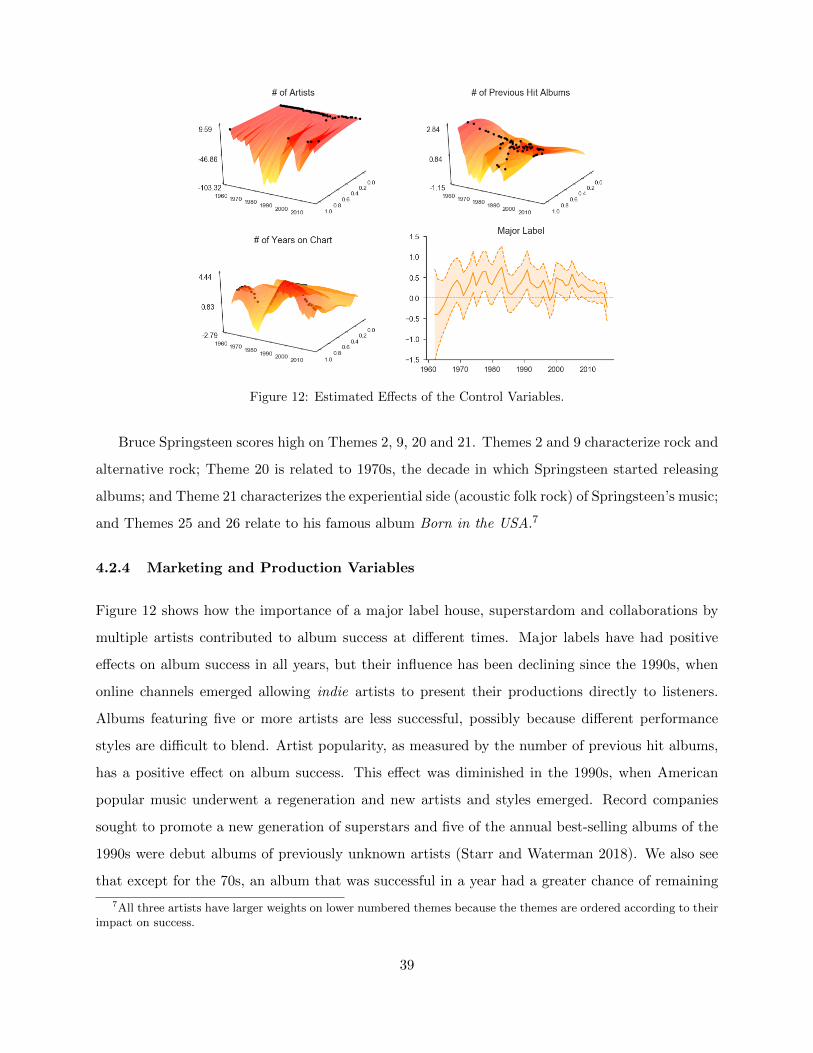
Figure 12: Estimated Effects of the Control Variables.

Bruce Springsteen scores high on Themes 2, 9, 20 and 21. Themes 2 and 9 characterize rock and

alternative rock; Theme 20 is related to 1970s, the decade in which Springsteen started releasing

albums; and Theme 21 characterizes the experiential side (acoustic folk rock) of Springsteen’s music;

and Themes 25 and 26 relate to his famous album Born in the USA.7

4.2.4 Marketing and Production Variables

Figure 12 shows how the importance of a major label house, superstardom and collaborations by

multiple artists contributed to album success at different times. Major labels have had positive

effects on album success in all years, but their influence has been declining since the 1990s, when

online channels emerged allowing indie artists to present their productions directly to listeners.

Albums featuring five or more artists are less successful, possibly because different performance

styles are difficult to blend. Artist popularity, as measured by the number of previous hit albums,

has a positive effect on album success. This effect was diminished in the 1990s, when American

popular music underwent a regeneration and new artists and styles emerged. Record companies

sought to promote a new generation of superstars and five of the annual best-selling albums of the

1990s were debut albums of previously unknown artists (Starr and Waterman 2018). We also see

that except for the 70s, an album that was successful in a year had a greater chance of remaining

7All three artists have larger weights on lower numbered themes because the themes are ordered according to theirimpact on success.

39

popular in subsequent years.

5 Album Recommendation and Playlist Design

We use our model to recommend albums that are congruent with the styles associated with specific

eras and to compile playlists that meet different design objectives. We now illustrate these uses.

Recommending Albums Holbrook and Schindler (1989) found that preferences for popular

music form around adolescence or early adulthood. How might we design albums for people of

different generations? One way is to base these recommendations on the dynamics of genres (x>i βt)

and the acoustical features (ft(ij)(aij)) in our model. According to our model, an album will score

differently across the years. We can therefore identify time periods (other than when it was released)

in which the album is predicted to have popular appeal. Figure 13 shows the predicted appeal of

three iconic albums in different years before and after their release: 1989 by Taylor Swift, Thriller

by Michael Jackson and Sgt. Pepper’s Lonely Hearts Club Band by the Beatles.

According to our model, 1989 reflects the tastes of the 80s and would have been successful if

it had launched in the late 80s and early 90. At least there is face validity for this prediction. In

an ABC news interview, Taylor Swift said that “The inspiration behind this record, I was listening

to a lot of late 80’s pop ... I really loved the chances they were taking, how bold it was . . . It was

apparently a time of limitless potential, the idea you could do what you want be what you want ...

the idea of endless possibility was kind of a theme in the last two years of my life.”

Thriller is considered as one of the best albums in music history. According to our model,

its musical style was most consistent with successful albums between 1970 and 1990. Thus it is

likely to be popular among listeners who grew up in this generation. The figure also shows that

it is unlikely to be as popular among people who grew up subsequently. Similarly, Sgt. Pepper’s

Lonely Hearts Club Band is also recognized to be one of the greatest albums of all time. Our model

suggests that todays successful music is not consistent with its style. Of course, it could continue

to appeal to the generation that grew up with it.

As an additional illustration, we take all albums that were released after 1995 and rank order

them based on their predicted score using the preference parameters for the year 1985. Table 8

40

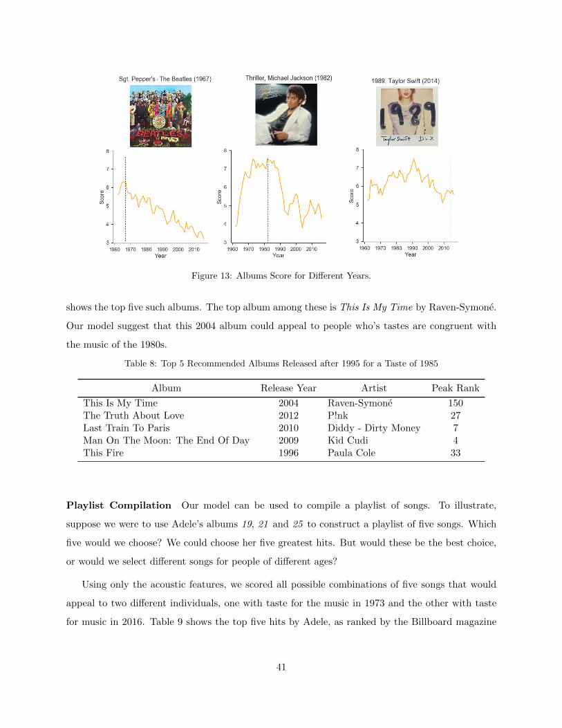
Figure 13: Albums Score for Different Years.

shows the top five such albums. The top album among these is This Is My Time by Raven-Symone.

Our model suggest that this 2004 album could appeal to people who’s tastes are congruent with

the music of the 1980s.

Table 8: Top 5 Recommended Albums Released after 1995 for a Taste of 1985

Album Release Year Artist Peak Rank

This Is My Time 2004 Raven-Symone 150The Truth About Love 2012 P!nk 27Last Train To Paris 2010 Diddy - Dirty Money 7Man On The Moon: The End Of Day 2009 Kid Cudi 4This Fire 1996 Paula Cole 33

Playlist Compilation Our model can be used to compile a playlist of songs. To illustrate,

suppose we were to use Adele’s albums 19, 21 and 25 to construct a playlist of five songs. Which

five would we choose? We could choose her five greatest hits. But would these be the best choice,

or would we select different songs for people of different ages?

Using only the acoustic features, we scored all possible combinations of five songs that would

appeal to two different individuals, one with taste for the music in 1973 and the other with taste

for music in 2016. Table 9 shows the top five hits by Adele, as ranked by the Billboard magazine

41

Figure 14: Acoustic Differences Between the Two Playlists: the Mean (a) and the Standard Deviation (b)of Each Acoustic.

critics8. It also shows the playlists our model recommends for the two individuals. The 1973 playlist

only has one song from Adele’s top five (Rolling in the Deep); the 2016 playlist has none. And the

playlists for 1973 and 2016 are also completely different. Figure 14 shows the means and standard

Table 9: Billboard’s Top 5 and Year Based Model Generated Compilations of Adele’s Songs.

Billboard’s Top 5 Songs Model Generated Compilations

– 1973 2016

Album Song Album Song Album Song

21 Rolling In The Deep 19 Cold Shoulder 19 First Love19 Chasing Pavements 19 Make You Feel My Love 25 Million Years Ago21 Someone Like You 19 Tired 21 Don’t You Remember25 Hello 25 Love in the Dark 21 He Won’t Go19 Hometown Glory 21 Rolling in the Deep 21 Lovesong

deviation of each acoustic fingerprint for the 1973 and 2016 playlists. The 1973 has longer songs,

and higher energy, key and mode compared to the 2016 playlist. It also contains a more diverse

collection of songs in terms of danceability, energy and time signature. The 2016 playlist has a

higher average acousticness, danceability, tempo and time signature.

8https://www.billboard.com/articles/columns/pop/8448730/adele-songs-best-ranked-critics-picks

42

6 Conclusion

In this paper, we developed a modeling framework to study the correlates of music success over the

past five decades. We used the model on data containing the genres, acoustical features, and crowd-

sourced tags of albums to understand how the impact of these variables have changed over the years.

The proposed model uses Bayesian nonparametric components of different types, including time-

varying penalized splines and a supervised hierarchical Dirichlet process, which flexibly capture the

impact of the acoustical features and tags, respectively. We found that all three sets of covariates

are important in explaining the relative success of albums.

Our model uncovered a number of interesting insights about the evolution of American popular

music. Some of our findings relate to broad trends in the popularity and decline of different genres

and the emergence of new forms of music. For instance, we found that Rock has remained the most

successful form of music in America, although its popularity has steadily declined, pop music is

almost as successful as hip hop, which took off in the early 80s and appears to have peaked in the

2000s. Rock music has tended to be more popular in periods when other forms of music were not;

hip hop’s success is positively correlated with most other types of music, except rock.

Focusing on the state-space dynamics associated with the acoustic signature of the albums, we

found that louder music has become more successful over time, with a peak occurring in the 80s.

Albums with slower tempo used to be more successful, but this changed after 2010 with the success

of artists like Taylor Swift, Gwen Stefani and Nickelback. Albums with songs that were recorded

in higher keys were more successful in the 60s; today, lower keys are more successful, as are fewer

key variations. Successful albums today have simpler compositions (lower average time signature)

and combine a few complex songs with several simple ones. Albums with longer songs have always

been less successful, but in recent years albums have done better if they have songs of different

lengths. Successful albums had music with high energy and low valence in the 60s, 70s and 80s,

when singers like Bob Dylan and Bruce Springsteen gave voice to the social turmoil and angst of

their times. Successful albums today have lower energy and low valence.

The supervised hierarchical Dirichlet process component of our model uncovered a number of

themes. These themes are probability distributions over the tags and represent how listeners

perceive and experience the albums. Themes emphasize different types of tags and can be

43

characterized as focusing on sub-genres (e.g., soft rock, new soul, jazz vocal), consumption contexts

(e.g., holiday, worship, party), emotions (e.g., love, anger), intensity (e.g., relaxing, kill for peace,

must hear), nostalgia (e.g., oldies, good times), mood (e.g., smooth, energetic, ambient), quality of

listening experience (e.g., virtuoso, deep lyrics, easy listening), type of experience (e.g., seen live,

own on vinyl) and other interesting aspects of music.

The time-varying parameters associated with the genres and acoustics are needed for describing

the evolution of tastes. They are also very important for recommending music and constructing

playlists. We used both the average levels and standard deviations of song acoustics to predict

the popularity of different compilation of songs. We showed how the model parameters can be

leveraged to predict the congruency of an album with the successful musical style of a particular

era. For instance, our model suggests that Taylor Swift’s 1989, produced in 2014, indeed reflects

the acoustical traits of successful albums of 1989. Such analysis can be useful for recommending

music to people who grew up in different times. We showed how our model can be useful for

compiling albums and playlists that take into account the acoustical balance of the collection. For

example, for someone interested in Adele’s songs, merely collecting (say) her top five hits would not

be as good as using songs that have the right acoustical balance. Similarly, playlists constructed

for today’s youth and people with the sensibility of the 70s would have different songs.

On the methodological level, we developed a novel nonparametric framework that captures the

information contained in data of different modalities. Our use of a supervised hierarchical Dirichlet

process for modeling text is new to the marketing literature, and our integration of different styles

of nonparametrics in a single model is a contribution to the relevant literatures is statistics and

computer science. Although constructed specifically for music, our model can also be used in other

experiential contexts where multi-modal data are available.

While we generated a number of substantive insights, it is also important to acknowledge some

limitations of our research. Our results describe how the music industry has evolved over time, but

we cannot assert causality about the effects of covariates because we used observational data. We

have also not tested the efficacy of our recommendations in real-life contexts. Finally, although our

model can be used for constructing playlists for listeners with different types of preferences, we did

not use individual-level playlist data and hence are unable to make individualized recommendations

that leverage user-specific parameters. Methodologically, we used MCMC methods for inference

44

because this allows proper quantification of uncertainty. But this can also be time consuming;

developing more scalable inference methods can be useful. We look forward to exploring these

opportunities and hope that researchers will use our model in other experiential contexts.

References

Alexander, Peter J (1996), ‘Entropy and popular culture: product diversity in the popular music

recording industry’, American Sociological Review 61(1), 171–174.

Anand, Narasimhan and Richard A Peterson (2000), ‘When market information constitutes fields:

Sensemaking of markets in the commercial music industry’, Organization Science 11(3), 270–284.

Ansari, Asim and Carl F Mela (2003), ‘E-customization’, Journal of marketing research 40(2), 131–

145.

Ansari, Asim and Raghuram Iyengar (2006), ‘Semiparametric thurstonian models for recurrent

choices: A bayesian analysis’, Psychometrika 71(4), 631.

Askin, Noah and Michael Mauskapf (2017), ‘What makes popular culture popular? product features

and optimal differentiation in music’, American Sociological Review 82(5), 910–944.

Bertin-Mahieux, Thierry, Douglas Eck, Francois Maillet and Paul Lamere (2008), ‘Autotagger: A

model for predicting social tags from acoustic features on large music databases’, Journal of New

Music Research 37(2), 115–135.

Bonnin, Geoffray and Dietmar Jannach (2015), ‘Automated generation of music playlists: Survey

and experiments’, ACM Computing Surveys (CSUR) 47(2), 26.

Bradlow, Eric T and Peter S Fader (2001), ‘A bayesian lifetime model for the “hot 100” billboard

songs’, Journal of the American Statistical Association 96(454), 368–381.

Bradlow, Eric T and Vithala R Rao (2000), ‘A hierarchical bayes model for assortment choice’,

Journal of Marketing Research 37(2), 259–268.

Bruner, Gordon C (1990), ‘Music, mood, and marketing’, The journal of Marketing pp. 94–104.

Chung, Tuck Siong, Roland T Rust and Michel Wedel (2009), ‘My mobile music: An adaptive

personalization system for digital audio players’, Marketing Science 28(1), 52–68.

Datta, Hannes, George Knox and Bart J Bronnenberg (2017), ‘Changing their tune: How

consumers’ adoption of online streaming affects music consumption and discovery’, Marketing

Science .

Dew, Ryan and Asim Ansari (2018), ‘Bayesian nonparametric customer base analysis with model-

based visualizations’, Marketing Science .

45

Dowd, Timothy J (2004), ‘Concentration and diversity revisited: Production logics and the us

mainstream recording market, 1940–1990’, Social forces 82(4), 1411–1455.

Elberse, Anita (2010), ‘Bye-bye bundles: The unbundling of music in digital channels’, Journal of

Marketing 74(3), 107–123.

Eliashberg, Jehoshua, Jedid-Jah Jonker, Mohanbir S Sawhney and Berend Wierenga (2000),

‘Moviemod: An implementable decision-support system for prerelease market evaluation of

motion pictures’, Marketing Science 19(3), 226–243.

Farquhar, Peter H and Vithala R Rao (1976), ‘A balance model for evaluating subsets of

multiattributed items’, Management Science 22(5), 528–539.

Giles, David E (2007), ‘Increasing returns to information in the us popular music industry’, Applied

Economics Letters 14(5), 327–331.

Hartman, WM (1997), ‘Signals, sound and sensation: Woodbury’, NY: American Institute of

Physics .

Holbrook, Morris B and Elizabeth C Hirschman (1982), ‘The experiential aspects of consumption:

Consumer fantasies, feelings, and fun’, Journal of consumer research 9(2), 132–140.

Holbrook, Morris B and Punam Anand (1990), ‘Effects of tempo and situational arousal on the

listener’s perceptual and affective responses to music’, Psychology of Music 18(2), 150–162.

Holbrook, Morris B and Robert M Schindler (1989), ‘Some exploratory findings on the development

of musical tastes’, Journal of Consumer Research 16(1), 119–124.

Iwanaga, Makoto (1995), ‘Relationship between heart rate and preference for tempo of music’,

Perceptual and motor skills 81(2), 435–440.

Juslin, Patrik N and Daniel Vastfjall (2008), ‘All emotions are not created equal: Reaching beyond

the traditional disputes’, Behavioral and Brain Sciences 31(5), 600–621.

Juslin, Patrik N and Petri Laukka (2004), ‘Expression, perception, and induction of musical

emotions: A review and a questionnaire study of everyday listening’, Journal of New Music

Research 33(3), 217–238.

Kim, Jin Gyo, Ulrich Menzefricke and Fred M Feinberg (2007), ‘Capturing flexible heterogeneous

utility curves: A bayesian spline approach’, Management Science 53(2), 340–354.

Koelsch, Stefan, Thomas Fritz, D Yves v. Cramon, Karsten Muller and Angela D Friederici (2006),

‘Investigating emotion with music: an fmri study’, Human brain mapping 27(3), 239–250.

Krueger, Alan B (2005), ‘The economics of real superstars: The market for rock concerts in the

material world’, Journal of Labor Economics 23(1), 1–30.

46

Lee, Jonathan, Peter Boatwright and Wagner A Kamakura (2003), ‘A bayesian model for prelaunch

sales forecasting of recorded music’, Management Science 49(2), 179–196.

Lena, Jennifer C (2006), ‘Social context and musical content of rap music, 1979–1995’, Social Forces

85(1), 479–495.

Lena, Jennifer C and Mark C Pachucki (2013), ‘The sincerest form of flattery: Innovation,

repetition, and status in an art movement’, Poetics 41(3), 236–264.

Li, Yang and Asim Ansari (2013), ‘A bayesian semiparametric approach for endogeneity and

heterogeneity in choice models’, Management Science 60(5), 1161–1179.

Nave, Gideon, Juri Minxha, David M Greenberg, Michal Kosinski, David Stillwell and Jason

Rentfrow (2018), ‘Musical preferences predict personality: evidence from active listening and

facebook likes’, Psychological science p. 0956797618761659.

Ocasio, William, Michael Mauskapf and Christopher WJ Steele (2016), ‘History, society, and

institutions: The role of collective memory in the emergence and evolution of societal logics’,

Academy of Management Review 41(4), 676–699.

Papies, Dominik and Harald J van Heerde (2017), ‘The dynamic interplay between recorded music

and live concerts: The role of piracy, unbundling, and artist characteristics’, Journal of Marketing

81(4), 67–87.

Peterson, Richard A and David G Berger (1975), ‘Cycles in symbol production: The case of popular

music’, American sociological review pp. 158–173.

Platt, John C, Christopher JC Burges, Steven Swenson, Christopher Weare and Alice Zheng (2002),

Learning a gaussian process prior for automatically generating music playlists, in ‘Advances in

neural information processing systems’, pp. 1425–1432.

Rossi, Peter (2014), Bayesian non-and semi-parametric methods and applications, Princeton

University Press.

Rossman, Gabriel (2012), Climbing the charts: What radio airplay tells us about the diffusion of

innovation, Princeton University Press.

Scherer, Klaus R (2004), ‘Which emotions can be induced by music? what are the underlying

mechanisms? and how can we measure them?’, Journal of new music research 33(3), 239–251.

Schmitt, Bernd H (2010), Customer experience management: A revolutionary approach to

connecting with your customers, John Wiley & Sons.

Serra, Joan, Alvaro Corral, Marian Boguna, Martın Haro and Josep Ll Arcos (2012), ‘Measuring

the evolution of contemporary western popular music’, Scientific reports 2, 521.

47

Sethuraman, Jayaram (1994), ‘A constructive definition of dirichlet priors’, Statistica sinica pp. 639–

650.

Shively, Thomas S, Greg M Allenby and Robert Kohn (2000), ‘A nonparametric approach to

identifying latent relationships in hierarchical models’, Marketing Science 19(2), 149–162.

Starr, Larry and Christopher Alan Waterman (2018), American popular music from minstrelsy to

MP3, Oxford University Press, USA.

Sun, Dongchu, Robert K Tsutakawa and Paul L Speckman (1999), ‘Posterior distribution of

hierarchical models using car (1) distributions’, Biometrika 86(2), 341–350.

Teh, Yee W, Michael I Jordan, Matthew J Beal and David M Blei (2005), Sharing clusters among

related groups: Hierarchical dirichlet processes, in ‘Advances in neural information processing

systems’, pp. 1385–1392.

Tobin, James (1958), ‘Estimation of relationships for limited dependent variables’, Econometrica:

journal of the Econometric Society pp. 24–36.

Ullman, Jeffrey David (2011), Mining of massive datasets, Cambridge University Press.

Vogel, Harold L (2014), Entertainment industry economics: A guide for financial analysis,

Cambridge University Press.

Wand, MP and JT Ormerod (2008), ‘On semiparametric regression with o’sullivan penalized

splines’, Australian & New Zealand Journal of Statistics 50(2), 179–198.

Wedel, Michel and Jie Zhang (2004), ‘Analyzing brand competition across subcategories’, Journal

of marketing research 41(4), 448–456.

Zentner, Marcel, Didier Grandjean and Klaus R Scherer (2008), ‘Emotions evoked by the sound of

music: characterization, classification, and measurement.’, Emotion 8(4), 494.

48

A Acoustic Fingerprints

We introduce each one of the acoustic fingerprints and provide a description of their meaning. The

objective acoustic measures are:

- Key: is an integer that maps a song to its corresponding pitch. A pitch is a property of

sound that allows to judge it as “high” or “low”. It is determined by the frequency of sound

wave vibration. It relates the fundamental frequency of a sound to a real number such that

the key can be represented by an integer from 0 to 11 with the note C=0, C]=1, and so on

till B = 11. The study of pitch perception has been a central entity in psychoacoustics that is

essential for representing, processing and perceiving sounds in the auditory system (Hartman

1997).

- Loudness: is a measure of the loudness of a track in decibels (dB). The loudness of a track

is the quality of sound that psychologically correlates with the physical strength of the song

(sound amplitude). Values of loudness range between 0 and -60dB with 0dB louder than

-60dB.

- Mode: is a dummy variable that indicates the modality of a song. 0 refers to the minor

modes and 1 to the major modes. Each mode is characterized by a musical scale of certain

melodic behaviors.

- Tempo: is the overall estimated tempo of a track in beats per second. The tempo

characterizes the speed and the pace of a given piece of music.

- Time signature: specifies how many beats are in each bar.

The subjective acoustic measures include:

- Acousticness: is a continuous measure between 0 and 1 that indicates how acoustic a song

is. Tracks with acousticness will consist mostly of natural acoustic sounds (e.g. guitar, piano,

orchestra, unprocessed human voice. Songs with low acousticness consist mostly of electric

sounds (e.g. electric guitar, synthesizers, etc.).

49

- Danceability: is a continuous measure between 0 and 1 that describes how suitable is a song

for dancing. The score is based on multiple musical elements including the song tempo and

its stability, beat strength and overall regularity.

- Energy: is a continuous measure between 0 and 1 that gives a level of confidence about the

intensity of a song. Songs with high energy are energetic tracks with fast pace, loud and

noisy.

- Instrumentalness: is a continuous measure that reports the confidence about the presence

of spoken words in a song. For example, Rap music has a low instrumentalness measure while

instrumental classical music has a high instrumentalness score.

- Liveness: is a probability measure that reports if a song was performed live.

- Speechiness: is a continuous measure that reports the confidence about the presence of

spoken words in a song. Audio books or poetry recordings have a score that is close to 1.

When a track has a speechiness score between 0.33 and 0.66, it indicates that the recording

may contain both spoken words and music (in parallel or in sections).

- Valence: is a continuous measure between 0 and 1that describes the positiveness of the

music that is conveyed by the song. Songs with high valence are more likely to convey more

positive emotions (e.g. happiness, joy, euphoria) while songs with low valence are more likely

to convey more negative emotions (e.g. anger, sadness, depression).

50