Journal of Sound and Vibration (1999) 222(1), 19–47Article No. jsvi.1998.1986, available online at http://www.idealibrary.com on

DYNAMIC STABILITY OF A ROTATING SHAFTDRIVEN THROUGH A UNIVERSAL JOINT

A. J. M J

Department of Mechanical Engineering and Applied Mechanics,The University of Michigan, G044 W.E. Lay Automotive Laboratory,

1231 Beal Avenue, Ann Arbor, MI, 48109-2121, U.S.A.

A. A

Department of Mechanical Engineering, The University of Michigan—Dearborn,4901 Evergreen Rd, Dearborn, MI, 48128-1491, U.S.A.

R. A. S

Department of Mechanical Engineering and Applied Mechanics,The University of Michigan, G044 W.E. Lay Automotive Laboratory,

1231 Beal Avenue, Ann Arbor, MI, 48109-2121, U.S.A.

(Received 11 May 1998, and in final form 21 September 1998)

The dynamic stability of a system composed of driving and driven shaftsconnected by a universal joint is investigated. Due to the characteristics of thejoint, even if the driving shaft experiences constant torque and rotational speed,the driven shaft experiences fluctuating rotational speed, bending moments andtorque. These are sources of potential parametric, forced and flutter typeinstabilities. The focus of this work is on the lateral instabilities of the driven shaft.Two distinct models are developed, namely, a rigid body model (linear andnon-linear) and a flexible model (linear). The driven shaft is taken to be pinnedat the joint end and to be resting on a compliant damped bearing at the otherend. Both models lead to sets of differential equations with time dependentcoefficients. For both rigid (linear and non-linear) and flexible models, flutterinstabilities were found but occurred outside the practical range of operation(rotational speed and torque) for lightly damped systems. Parametric instabilitycharts were obtained by using the monodromy matrix technique for both rigid andflexible linear models. The transmitted bending moments were found to causestrong parametric instabilities in the system. By comparing the results from thetwo linear models, it is shown that the inclusion of flexibility leads to new zonesof instability, not predicted by previous models. These zones, depending on thephysical parameters of the system, can occur for practical conditions of operation.Using direct numerical integration for a few sets of specific parameter values,forced resonances were found when the rotational speed reached a value equal toa natural frequency of the system divided by two.

7 1999 Academic Press

0022–460X/99/160019+29 $30.00/0 7 1999 Academic Press

. . .20

1. INTRODUCTION

Universal joints, commonly referred to as U-Joints, are widely used in rotarymachines when transmission of torque or power is needed between two shafts thatare not collinear. Although a non-constant velocity joint, the U-Joint is extensivelyused in preference to other types of joints. The principal advantages of it are itsrelatively low manufacturing cost, simple and rugged construction, long life, andease of serviceability. Also, in addition to providing the necessary torque capacityin a limited operating space, the U-Joint has the capability to withstand relativelyhigh externally imposed axial forces and relatively high operational speeds.

In systems driven by U-Joints, instabilities of several types can occur, forexample, flutter, parametric, and forced. To fully analyze these instabilitiesmechanical models involving U-Joints and rotating shafts need to be developedincorporating the physics which produce the instabilities.

The present work deals with the dynamic stability of rigid and flexible shaftsmounted in a compliant damped support and driven through a U-Joint. The focusis on the lateral instabilities of the shaft, and the effects of bearing compliance anddamping and system geometric parameters.

A brief review of the salient literature will now be given.The literature on rotating shafts is very extensive, because of the numerous

technical applications. Citations to early work can be found in H. P. Lee et al.[1], in their paper on a rotating Timoshenko shaft. The recent work of C. W. Leeand Yun [2] should also be noted. Guidelines to some of the modelling employedhere were obtained from the work of Eshleman and Eubanks [3] on the criticalspeeds of rotating shafts.

The literature on stability, and the use of follower and non-follower forces andmoments, is equally extensive. The classic works of Ziegler [4] and Leipholz [5]contain numerous instructive examples. The field continues to be fruitful, as theworks of Khader [6] on follower loads, Plaut and Wauer [7] on parametric,external and combination resonances, and the text by C. W. Lee [8] attest.

Work on drive systems containing U-Joints is not so extensive. Lateral andtorsional vibrations of a rotating shaft driven by a universal joint were investigatedby Ota et al. [9, 10]. There the moment applied by the U-Joint to the driven shaftwas modelled as a non-follower one. The driven shaft was taken to be a masslessflexible shaft with an off-center symmetric rotor. The flexibility of the shaft wasincluded in the formulation as a lumped stiffness, rather than distributed.Parametric resonances were found to be possible when the angular velocity of thedriving shaft was close to an even integer (or sub-multiple) of a torsional or lateralnatural frequency of the driven shaft. In a later work [11] Kato and Otainvestigated the lateral vibrations of a rotating shaft driven by a U-Joint withfriction, the moment due to the friction being modelled as a non-follower one.

The effects of joint angles and joint friction in a double universal joint systemwere investigated by Sheu et al. [12]. Using Rayleigh beam theory they found thatthe values of the critical speeds for the intermediate shaft are affected by the axialtorques, which depend on viscous friction coefficients and joint angles.

Saigo et al. [13] considered the dynamics of a multi shaft, multi U-Joint system.They showed that Coulomb friction in one of the U-Joints could lead to unstable

21

motions. However, the shafts were treated as rigid and the fluctuations ofrotational speeds due to the U-Joint were taken to be negligible. Also, theirmodelling is such that time dependent coefficients do not appear in the equationsof motion so parametric instabilities can not be addressed.

Torsional instabilities, due to fluctuating angular velocity, in a drivelineimcorporating a U-Joint were investigated by Asokanthan and Hwang [14] andAsokanthan and Wang [15]. The system was modelled as a two-degree-of-freedomsystem with damping. Analytical conditions for the onset of parametric instabilitywere derived and the occurrence of combination resonance of the sum type wasidentified while the combination resonance of the difference type was shown to beabsent. Damping was found to stabilize the system in the sub-harmonic case andto destabilize the system in the combination case. For a given joint angle thecritical speed ranges to be avoided for stable operation were obtained. Based onthese works it is seen that both torsional and lateral instabilities can occur inU-Joint systems. In the present work the focus is on shafts whose properties aresuch that the bending natural frequencies are much less than the torsional naturalfrequencies. Hence, torsional motions are neglected.

The influence of joint angle on the critical speed behavior of a shaft driventhrough a U-Joint was investigated by Rosenberg [16]. In that work the shaft wasmodelled as a massless uniform elastic shaft with a concentrated mass at itsmidpoint. The transmitted torque was taken to be a follower one. There the onlybending moments considered were those due to bending components of thefollower torque, whereas a U-Joint also produces direct bending components. Itwas found that when the joint angle was different from zero, parametricinstabilities could arise.

Transverse vibrations and stability of a rigid driven shaft in a U-Jointsystem with springs and dampers and zero initial joint angles were analyzedby Iwatsubo and Saigo [17]. It was found that parametric and flutter typeinstabilities could arise. The relative role of system damping and stiffness wasinvestigated.

Several possibly important issues have not so far been addressed in theliterature, to the authors’ knowledge. Most importantly, the effects of distributedshaft flexibility and inertia on parametric resonances have not been explored. Also,effects of non-zero initial joint angles and system non-linearities need to beassessed. These issues are explored in this paper, with the major emphasis beingon the role of distributed shaft flexibility and inertia.

The plan for the paper is as follows. Section 2 introduces a model, similarto Iwatsubo and Saigo’s model, in which the driven shaft is regarded asrigid. However, the initial joint angles are taken to be non-zero and somenon-linear effects are taken into account. In Section 3 a flexible model (linear) forthe driven shaft is developed. Galerkin’s method is applied to the equations ofmotion for the flexible model in Section 4. In sections 5 and 6 flutter typeinstabilities and parametric type instabilities are examined for both models.Section 7 gives some preliminary results for the rigid non-linear model, obtainedusing direct numerical integration, and in section 8 forced resonances areinvestigated.

Driven shaftDriving shaft

Connector (Yoke)

Cross piece

A

Z

X

l

Y

C

B

. . .22

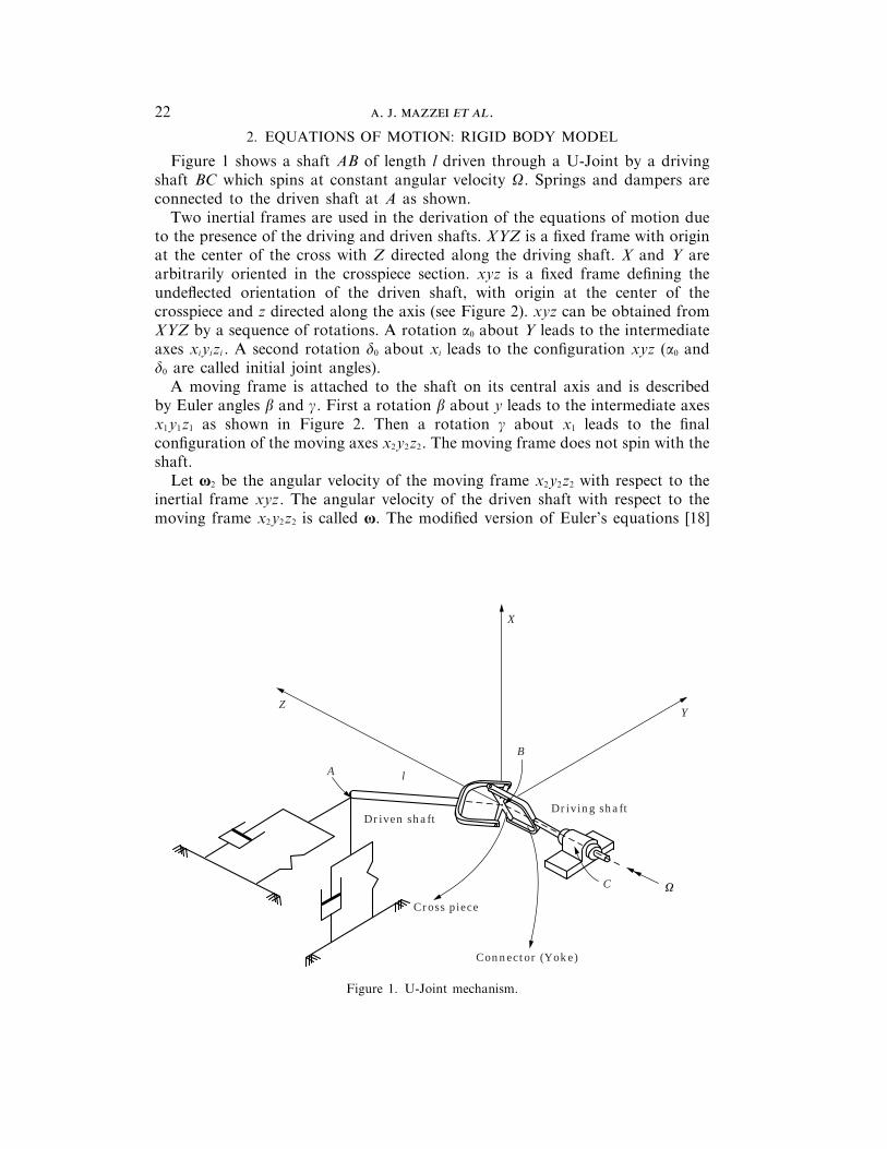
2. EQUATIONS OF MOTION: RIGID BODY MODEL

Figure 1 shows a shaft AB of length l driven through a U-Joint by a drivingshaft BC which spins at constant angular velocity V. Springs and dampers areconnected to the driven shaft at A as shown.

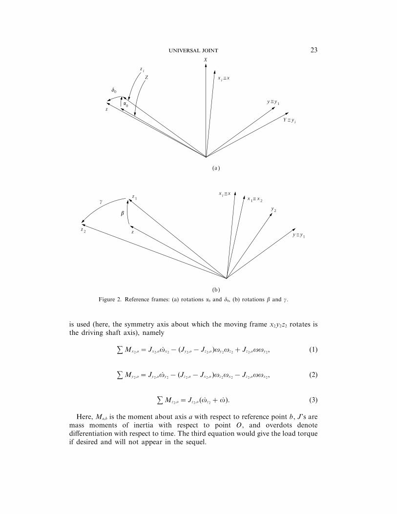
Two inertial frames are used in the derivation of the equations of motion dueto the presence of the driving and driven shafts. XYZ is a fixed frame with originat the center of the cross with Z directed along the driving shaft. X and Y arearbitrarily oriented in the crosspiece section. xyz is a fixed frame defining theundeflected orientation of the driven shaft, with origin at the center of thecrosspiece and z directed along the axis (see Figure 2). xyz can be obtained fromXYZ by a sequence of rotations. A rotation a0 about Y leads to the intermediateaxes xiyizi . A second rotation d0 about xi leads to the configuration xyz (a0 andd0 are called initial joint angles).

A moving frame is attached to the shaft on its central axis and is describedby Euler angles b and g. First a rotation b about y leads to the intermediate axesx1y1z1 as shown in Figure 2. Then a rotation g about x1 leads to the finalconfiguration of the moving axes x2y2z2. The moving frame does not spin with theshaft.

Let v2 be the angular velocity of the moving frame x2y2z2 with respect to theinertial frame xyz. The angular velocity of the driven shaft with respect to themoving frame x2y2z2 is called v. The modified version of Euler’s equations [18]

Figure 1. U-Joint mechanism.

zi

Z

z

X

xi x=

y y1=

Y yi=

0

0

(a)

zz2

z1xi x=

x1 x2=

y2

y y1=

(b)

23

Figure 2. Reference frames: (a) rotations a0 and d0, (b) rotations b and g.

is used (here, the symmetry axis about which the moving frame x2y2z2 rotates isthe driving shaft axis), namely

s Mx2,o = Jx2,ovx2 − (Jy2,o − Jz2,o )vy2vz2 + Jz2,ovvy2, (1)

s My2,o = Jy2,ovy2 − (Jz2,o − Jx2,o )vz2vx2 − Jz2,ovvx2, (2)

s Mz2,o = Jz2,o (vz2 + v). (3)

Here, Ma,b is the moment about axis a with respect to reference point b, J’s aremass moments of inertia with respect to point O, and overdots denotedifferentiation with respect to time. The third equation would give the load torqueif desired and will not appear in the sequel.

. . .24

Here,

v2 = b� cos (g)j 2 − b� sin (g)k 2 + gi 2 (4)

and

v2 = gi 2 + (b� cos (g)− b� g sin (g))j 2 − (b� sin (g)+ b� g cos (g))k 2, (5)

where i 2, j 2 and k 2 denote unit vectors in the x2, y2, and z2 directions, respectively.Assuming that the initial joint angles are small, such as usually occurs in

practice, the rotational speed of the driven shaft can be written as (see, forexample, reference [19]):

v0Vp2(t)=V$1−a2

0

2(1−cos (2Vt))−

d20

2(1+cos (2Vt))− a0d0 sin (2Vt)%,

(6)

where V is the rotational speed of the driving shaft.Substitution of equations (4), (5) and (6) into equations (1) and (2) leads to

s Mx2,o = Jx2,og+(Jy2,o − Jz2,o )b�2 cos (g) sin (g)+ Jz2,ob� cos (g)Vp2(t), (7)

s My2,o = Jy2,o (b� cos (g)− b� g sin (g))+ (Jz2,o − Jx2,o )b� g sin (g)− Jz2,ogVp2(t).

(8)

The next step is to calculate the moments resolved on the moving system. Herethe driven shaft is taken to be pinned at the end coinciding with the U-Joint centerand to rest on a compliant bearing at the other end. The bearing is modelled bypairs of springs and dampers (see Figure 1).

In the model used here the spring and damper forces are given by

Fs =−Kxl sin (b)i 2 +Kyl sin (g) cos (b)j 2, (9)

Fd =−Cxlb� cos (g)i 2 +Cylgj 2, (10)

where K stands for spring stiffness and C stands for the viscous dampingcoefficient.

For two perpendicular springs (Kx , Ky ) and two perpendicular dampers (Cx , Cy )directed along x and y, respectively, the moments that arise at the center of theU-Joint can be expressed as

Mso =−(l2Ky sin (g) cos (b))i 2 − (l2Kx sin (b))j 2, (11)

Mdo =−(l2Cyg)i 2 − (l2Cxb� cos (g))j 2. (12)

25

The next step is to obtain the components of the moment transmitted by theU-Joint. The transmitted moment acts along the normal unit vector to thecrosspiece (see, for example, reference [19]) which is given by

en = enx2i 2 + eny2j 2 + enz2k 2, (13)

where

enx2 =−1o

[cos (t)b−cos (t)a0gd0 + cos (t)a0 − sin (t)g−sin (t)d0]

× [cos (t)− cos (t)ba0 + sin (t)ba0], (14)

eny2 =−1o

[cos (t)b−cos (t)a0gd0 + cos (t)a0 − sin (t)g− sin (t)d0]

× [cos (t)gb+cos (t)a0d0 + cos (t)a0g+sin (t)− sin (t)gd0], (15)

enz2 0 o=X[cos (t)gb+cos (t)a0d0 + cos (t)a0g+sin (t)− sin (t)gd0]2

+ [cos (t)− cos (t)ba0 + sin (t)bd0]2(16)

and t=Vt.The moment that the U-Joint applies to the driven shaft is

M=Men , (17)

where M can be shown to be related to the torque that acts on the driving shaft,T0, by

M=T0

en · K, (18)

in which K denotes the unit vector in the Z direction.Substitution of equations (4), (5), (11), (12), (17) and (18) in equations (1) and

(2) leads to the following set of non-linear ordinary differential equations:

n2g� +(1− h)b� 2n2 cos (g) sin (g)+ hb� n2 cos (g)p2(t)

= M x2 −K y sin (g) cos (b)−C yng, (19)

n2b� cos (g)+ (h−2)b� gn2 sin (g)− hgn2p2(t)= My2 −K x sin (b)−C ynb� cos (g),

(20)

where the following non-dimensional quantities have been introduced: n=V/V0;V0 being a reference frequency (taken as the first bending frequency of anon-rotating beam pinned at both ends, for facility of comparison with the flexiblemodel). The overdot now stands for d/dt, h= Jz2,o /J, J= Jx2,o = Jy2,o , p2(t) isobtained from equation (6) and K x = l2Kx /(JV2

0 ), K y = l2Ky /(JV20 ), C x = l2Cx /(JV0),

C y = l2Cy /(JV0), M x2 =Mx2/(JV20 ), M y2 =My2/(JV2

0 ). M x2 and M y2 are verycomplicated functions and details are not given. They are handled using MAPLE[20] in the results given later using the non-linear model.

. . .26

Assuming that the deflections at the bearings are small, one can use small angleapproximations. The following linear model is then obtained:

n26gb� 7+ n$ C y2

−hnp2(t)hnp2(t)

C x2 %6gb� 7+$K y

00K x%6gb7+G$ 0

−110%6gb7

+ G sin (2t)$−10

01%6gb7+G cos (2t)$01 1

0%6gb7= G$ sin (2t)

1−cos (2t)−(1+cos (2t))

−sin (2t) %6d0

a07, (21)

where G=T0/(2JV20 ).

An analysis of these equations reveals the presence of the direct bendingmoments transmitted by the U-Joint. They appear on the fourth, fifth and sixthterms of the set of equations. The fifth and sixth terms involve time dependentcoefficients and can lead to parametric resonances. The fourth term can lead toflutter type instabilities. The right-hand sides of the equations are due to theinclusion of the initial joint angles in the formulation and can lead to forcedmotion resonances.

The homogeneous parts of equations (21) lead to a model similar to oneobtained by Iwatsubo and Saigo [17], if one neglects second order effects such asa2

0 , d20 and a0d0. Iwatsubo and Saigo’s model does not contain these second order

effects because the fluctuation of the angular velocity of the driven shaft was nottaken into account (which is the same as using the approximation p2(t)=1).Moreover, since in their work the initial joint angles are not included, the forcingterms that are present in equations (21) do not appear.

In the sequel the numerical results presented are for the linear model, exceptwhere otherwise noted.

3. EQUATIONS OF MOTION: FLEXIBLE MODEL

Here the equations of motion are developed with respect to an inertial frame,namely the frame xyz of section 2. This is essentially the ‘‘shadow beam’’approach, with the z-axis directed along the shaft (treated as rigid) axis. The mainmodelling features are as follows.

The Rayleigh beam theory is used (in the sequel only slender shafts are treated,so shear deformations are taken to be negligible). Elastic transverse deformationsu and v of the neutral axis are measured with respect to xyz. If the driven shaftwere rigid it would rotate at an angular velocity v about its axis. In Rayleigh beamtheory kinematics, a cross-sectional area disk (disk of thickness Dz andcross-sectional area A) is treated as rigid. The angular velocity of that disk is takento be

vD =−12v

1z 1ti +

12u1z 1t

j +vk .

27

Axial and torsional displacements are neglected, since the associated frequenciesare much higher than the bending frequencies for the examples studied.

A major issue is the treatment of the moment M transmitted by the U-Joint tothe driven shaft. This moment is known to be along the normal vector to thecrosspiece, which in turn depends on the orientation of the driven shaft. If oneincludes the instantaneous slopes due to deformation at the U-Joint end, one canwrite ( f denotes a functional form; a0 and d0 are the initial joint angles)

M=Men = f 0a0 +1u1z bz=0

, d0 −1v1z bz=01. (22)

Resolving M along the xyz axes, leads to two bending moments Mx and My andone twisting torque Mz . At this juncture several approaches are possible, namely

(1) The slopes 1u/1z=z=0, 1v/1z=z=0 could be neglected in equation (22). This canbe shown to lead to a forced motion problem only. The bending momentswould not cause any parametric instabilities.

(2) The torque could be treated as acting along the deformed configuration (asdone by Rosenberg [16]), with the bending moments handled as described in(1). It was found that this approach led only to weak parametric instabilities.Since the parametric instabilities in an actual laboratory model (specificationsgiven later) were quite strong, this approach was abandoned.

(3) The deformation slopes in equation (22) are retained. This, as the sequel willshow, leads to the physically observed feature of strong parametricresonances. Thus, approach (3) is used. Also, following Rosenberg’s work,the torque was taken to act along the deformed configuration. Note that thebending moments are incorporated into the model by treating them as pointcouples acting at the U-Joint, handled mathematically by Dirac deltafunctions.

Less problematical modelling features are: the springs (bearings) are treated bythe appropriate choice of Galerkin functions; the dampers (bearings) are modelledas linear viscous dampers, treated as point forces handled mathematically by Diracdelta functions.

With the above assumptions the non-dimensional equations of motion can beshown to be (see reference [19]):

EI14u1z4 + rA

12u1t2 +Fdx +

1Mby

1z+T

13v1z3 =

14

rAR2 0 14u1z2 1t2 +2v

13v1z2 1t1, (23)

EI14v1z4 + rA

12v1t2 +Fdy −

1Mbx

1z−T

13u1z3 =

14

rAR2 0 14v1z2 1t2 −2v

13u1z2 1t1, (24)

where Fdx , Fdy are external damping forces per unit length, Mbx and Mby are externalbending moments per unit length, v is the angular velocity of the driven shaft(treated as rigid) and is given by equation (6). Also, E denotes Young’s modulus,

. . .28

I the area moment of inertia, r the mass density, A the cross-sectional area andR the cross-sectional radius.

These equations are subjected to the boundary conditions

u= v= u0= v0=0, z=0; u0= v0=0, z= l;

EIu1=Kxu, z= l; EIv1=Kyv, z= l. (25)

The bending moments transmitted by the U-Joint are given by

Mx =T0

2 $0d0 −1v1z bz=01 sin (2Vt)−0a0 +

1u1z bz=01(1+cos (2Vt))%, (26)

My =T0

2 $0d0 −1v1z bz=01(1−cos (2Vt)−0a0 +

1u1z bz=01 sin (2Vt))%. (27)

Consequently,

Mbx =MxD(z), Mby =MyD(z),

where D stands for the Dirac delta function.The transmitted torque is given by (the magnitude is taken to be constant along

the shaft)

T=T0p1(t)=T0$1+a2

0

2(1−cos (2Vt))+

d20

2(1+cos (2Vt))+ a0d0 sin (2Vt)%.

(28)

Also

Fdx =Cx1u1t bz= l

D(z− l), Fdy =Cy1v1t bz= l

D(z− l).

Introducing the dimensionless variables and parameters: U= u/l, V= v/l,Z= z/l, L(Z)= lD(z), n=V/V0, V0 = (p2/l2)zEI/(rA) (the lowest bendingfrequency of a non-rotating pinned–pinned Euler–Bernoulli beam), G1 =T0/(rAV2

0 l3), X2 =EI/(rAV20 l4), X3 =R2/(4l2), X4 =2X3, d1 =Cx /(rAV0l), d2 =Cy /

(rAV0l), then, using equations (26), (27) and (28), equations (23) and (24) become

X214U1Z4 + n2 12U

1t2 + d1n1U1t bZ=1

L(Z−1)+G113V1Z3 p1(t)−X3n

2 14U1Z2 1t2

−X4n2p2(t)

13V1Z2 1t

−G1

21V1Z bZ=0

(1−cos (2t))d(L(Z))

dZ−

G1

21U1Z bZ=0

× sin (2t)d(L(Z))

dZ=

G1

2d(L(Z))

dZ[a0 sin (2t)− d0(1−cos (2t))], (29)

29

X214V1Z4 + n2 12V

1t2 + d2n1V1t bZ=1

L(Z−1)−G113U1Z3 p1(t)−X3n

2 14V1Z2 1t2

+X4n2p2(t)

13U1Z2 1t

+G1

21U1Z bZ=0

(1+cos (2t))d(L(Z))

dZ+

G1

21V1Z bZ=0

× sin (2t)d(L(Z))

dZ=

G1

2d(L(Z))

dZ[d0 sin (2t)− a0(1+cos (2t))]. (30)

4. GALERKIN’S METHOD

The solutions are assumed to have the following form

U= sa

i=1

Fi (Z)Fi (t), V= sa

i=1

Ci (Z)Gi (t).

Application of Galerkin’s method leads to

n2$[g1mi ]−X3[l1mi ][0]

[0][g2mi ]−X3[l2mi ]%6{F� i}{G� i}7

+ n$ d1[j1mi ]np2(t)X4[l4mi ]

−np2(t)X4[l3mi ]d2[j2mi ] %6{F� i}{G� i}7

+$X2[a1mi ][0]

[0]X2[a2mi ]%6{Fi}

{Gi}7+G1$ [0]

−[d2mi ]− p1(t)[b2mi ][d3mi ]+ p1(t)[b1mi ]

[0] %6{Fi}{Gi}7

+G1 sin (2t)$[d1mi ][0]

[0]−[d4mi ]%6{Fi}

{Gi}7+G1 cos (2t)$ [0]

−[d2mi ]−[d3mi ]

[0] %6{Fi}{Gi}7

=

G1

2(d0(1−cos (2t))− a0 sin (2t)){F'm (0)}

G1

2(a0(1+cos (2t))− d0 sin (2t)){C'm (0)}

,gG

G

F

fhG

G

J

j

i=1, 2, 3, . . . , a, m=1, 2, 3, . . . , a. (31)

The coefficients in the above equations are listed in Appendix A.

. . .30

The first matrix on the left-hand side of equation (31) is the ‘‘mass’’ matrix andhas constant coefficients. The second matrix is due to the damping in the system(main diagonal terms) and to gyroscopic effects (cross diagonal terms). Asevidenced by the presence of p2(t), each gyroscopic term has a constant part plusa part that is a function of time. The third matrix is the ‘‘stiffness’’ matrix andhas constant coefficients. The fourth matrix has constant and time dependentelements. The time dependent coefficients are contained in the term p1(t) (seeequation (28)) and are second order effects. The constant parts of these elementsare due to the constant parts of the bending moments from the U-Joint and thefollower torque. This matrix can lead to flutter type instabilities and to parametricinstabilities (due to p1(t)). The fifth and sixth matrices of equation (31) arefunctions of time. These terms can lead to strong parametric resonances (as willemerge). The forcing term on the right-hand side of equation (31) is due to theinclusion of the initial joint angles (a0 and d0) in the formulation and can lead toforced motion type resonances.

The choice of Galerkin functions will now be discussed. Recall that the dampingforces and the moments applied by the U-Joint do not arise in the boundaryconditions. They are incorporated in the equations of motion via Dirac deltafunctions. However, as seen in equation (25), the spring forces do arise in theboundary conditions. Consequently, the Galerkin functions chosen are the modeshapes of a non-rotating Euler–Bernoulli beam pinned at one end and springsupported at the other end. Thus, the functions for the xz and yz planes are,respectively,

Fi (Z)= sinh (H(x)iZ)+sinh (H(x)i )sin (H(x)i )

sin (H(x)iZ), (32)

Ci (Z)= sinh (H(y)iZ)+sinh (H(y)i )sin (H(y)i )

sin (H(y)iZ), (33)

where H(x)i and H(y)i are the positive solutions of the following transcendentalequation:

H3[tan (H)− tanh (H)]−2KL3

EItanh (H) tan (H)=0, (34)

for K=Kx and K=Ky , respectively. Note that these Galerkin functions satisfyall the conditions (25).

The Galerkin coefficients involve integrals containing products of hyperbolicfunctions and are calculated by a MAPLE routine for a given value of N (the seriestruncation value). Direct use of equations (32) and (33) led to numerical problemsin MAPLE because of excessively large values of the integrands. This problem wasresolved by using a set of normalized functions:

F*i (Z)=Fi (Z)

Fi (Z)=Z=1, C*i (Z)=

Ci (Z)Ci (Z)=Z=1

.

31

5. FLUTTER INSTABILITIES

Neglecting the time dependent coefficients and using the approximation p2 3 1(since a0 and d0 are small), the homogeneous part of equation (21), for the rigidbody model, reduces to

n26gb� 7+ n$ C y2

−hn

hn

C x2%6gb� 7+$ K y

−G

G

K x%6gb7=6007. (35)

Similarly, for the flexible model, the homogeneous part of equation (31) reducesto

.. .n2[M ]{Q }+ n[D ]{Q }+[S ]{Q }= {0}, (36)

where

[M ]=$[g1mi ]−X3[l1mi ][0]

[0][g2mi ]−X3[l2mi ]%, [D ]=$ d1[j1mi ]

nX4[l4mi ]−nX4[l3mi ]

d2[j2mi ] %,[S ]=$ X2[a1mi ]

−G1[d2mi ]−G1[b2mi ]G1[d3mi ]+G1[b1mi ]

X2[a2mi ] %, {Q }=6{Fi}{Gi}7. (37)

Both equations (35) and (36) are approximate equations which permit fairlysimple, non-computationally intensive methods to be employed for exploringflutter instabilities. It will be shown later that the results so obtained are highlyaccurate, as seen by comparisons with the results obtained by the monodromymatrix method, which is exact.

Flutter instabilities occur whenever the associated eigenvalues of equations (35)or (36) have a positive real part.

During some numerical simulations it was discovered that both systems areunstable for all values of rotational speed and torque if the damping is zero. Thisis a rather alarming result at first glance but, as will be shown shortly, it is of nopractical consequence. Note that this also occurs in the model developed byIwatsubo and Saigo [17].

The instability for C=0 can be readily seen in the case C x =C y =C andK x =K y =K . For the rigid body case, taking solutions of the form

g= g0 elt, b= b0 elt,

equation (35) leads to a root for l:

l=12n

[−C + hnI+z(C 2 − n2h2 −4K )+ (4G−2C nh)I]

where I=z−1. When C =0, the real part of this complex number is alwayspositive and so the system is unstable in the entire parameter space of n and G.

Consider now the case where C $ 0. A numerical illustration will be given,hereafter referred to as the ‘‘laboratory model’’ (the terminology is based on anactual model that was built). The parameter values are a0 = d0 =10°,

0.0045

0.0040

0.0035

0.0030

0.0025

0.0020

0.0015

0.0010

0.0005

0.00004 5 6 73210

Non-dimensional rotational speed,

No

n-d

imen

sio

na

l to

rqu

e,

0.0045

0.0040

0.0035

0.0030

0.0025

0.0020

0.0015

0.0010

0.0005

0.00004 5 6 73210

Non-dimensional rotational speed,

No

n-d

imen

sio

na

l to

rqu

e (s

am

e a

s ri

gid

mo

del

),

. . .32

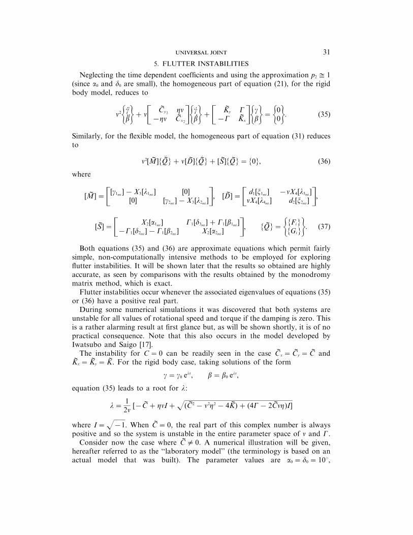
Figure 3. Flutter instability: rigid body laboratory model.

l=4·6×10−1 m, E=2·07×1011 N/m2, r=7·83×103 kg/m3, R=2·40 ×10−3 m, h=3·96×10−5, I=2·53×10−11 m4 (Ixx = Iyy = I= pR4/4), Kx =25·17 N/m and Ky =7·74 N/m. For this model a value of Cx =Cy =1×10−3 N/(m/s) was assumed. By direct numerical integration of equation (35), subjected tosome initial conditions, a logarithmic decrement procedure led to z1 1 z2 =0·001(z1, z2 are the non-dimensional damping ratios associated with g and b,respectively).

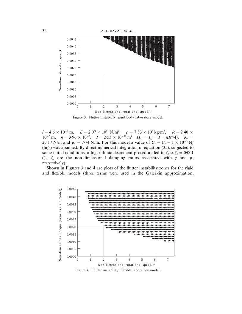
Shown in Figures 3 and 4 are plots of the flutter instability zones for the rigidand flexible models (three terms were used in the Galerkin approximation,

Figure 4. Flutter instability: flexible laboratory model.

33

sufficient for convergence) in torque-rotational speed space. Limits of practicaloperation are also shown as boxes in the lower left-hand corners of Figures 3 and4. The maximum attainable rotational speed of the laboratory model is judged tobe 5000 rpm, which gives n=2·0. The value (non-dimensional) of the staticallyapplied torque which would cause the shaft to yield (static yielding) is G=0·0042.The static torque which would cause a 10° angle of twist is G=0·0021 and thisis chosen as the limit of the practical torque range.

The main conclusion to be drawn is that the very light damping used moves theflutter instability zones outside the range of practical operation for both models.Similar results were found for other sets of parameter values.

6. PARAMETRIC INSTABILITIES

When the forcing terms are neglected, equations (21) and (31) are sets ofMathieu–Hill equations. Several approaches for the determination of the regionsof parametric instability of such equations exist in the literature.

Throughout this work the regions of instability are obtained by a numericaltechnique based on the so-called monodromy matrix (see reference [21]). Themonodromy matrix technique is very computationally intensive, but offers someadvantages over perturbation techniques and Hill’s infinite determinant. Forinstance, the method does not involve any approximations and is able to captureall instabilities within a parameter range (to within numerical accuracy).

Very briefly put, the technique is as follows. The equations of motion are castinto a first order form:

{q(t)}=[A(t)]{q(t)}, (38)

where the matrix [A(t)] is T*-periodic. The fundamental matrix is denoted by

[U(T*)]= [{q1(T*)}, {q2(T*)}, . . . , {qn (T*)}],

where {q1(t)}, {q2(t)}, . . . , {qn (t)} are any n linearly independent solutions of thesystem. Integrating equation (38) n times from 0 to T* with the n initial conditions

1 0 · · · 0

0 1 · · · 0GG

G

K

k

GG

G

L

l

[U(0)]= ······

· · ····

= [I]

0 0 · · · 1

generates a matrix [S], the monodromy matrix, given by [S]= [U(T*)]. Then theeigenvalues of [S], sj , are determined. The system is stable when >sj>E 1,j=1, 2, . . . , n. The process is repeated for every pair of n and G to cover the entireparameter space of interest.

In the zero damping case, parametric resonances are expected to emanate at zerotorque (G=0), from (so-called principal zones)

n=nni

j, i=1, 2, 3 . . . , j=1, 2, 3 . . . , (39)

0.0012

0.0010

0.0008

0.0006

0.0004

0.0002

0.00000.08 0.10 0.12 0.140.060.040.020.00

Non-dimensional rotational speed,

No

n-d

imen

sio

na

l to

rqu

e,

IV

I III II

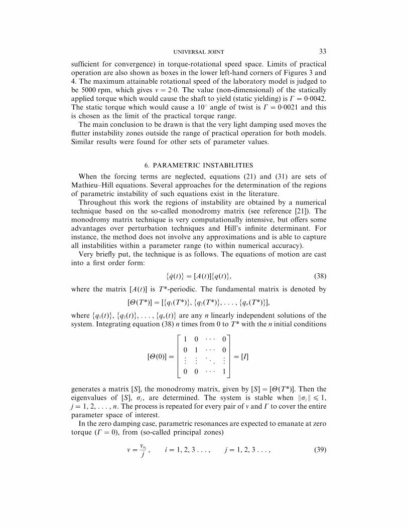
. . .34

Figure 5. Parametric instability: rigid body laboratory model.

where the nni’s are the non-dimensional natural frequencies of the rotating shaft(nn =Vn /V0, the Vn being the natural frequencies of the rotating shaft).

Combination parametric resonances may also occur. These emanate, at G=0,from the points (for zero damping)

n= bnni 2 nnj

2k b, i=1, 2, 3 . . . , j=1, 2, 3 . . . , k=1, 2, 3 . . . . (40)

Note that damping will shift the points of emanation to values of Gq 0.In general, the rigid body model has two natural frequencies; these correspond

to the shaft bouncing on the springs in two planes. These frequencies are functionsof the shaft’s rotational speed. Specifically, one frequency increases with therotational speed and is called the forward precessional frequency, and the seconddecreases with the rotational speed and is called the backward precessionalfrequency. Note that for the examples treated here the difference between therotating and non-rotating frequencies is negligible. In the flexible model thefrequencies will also be influenced by rotation but, again, the differences werefound to be negligible. The first two modes of the flexible system are nearlyidentical to the rigid body modes since the spring stiffness is very small comparedto the shaft stiffness. These two modes will be referred to as ‘‘predominantly rigidmodes’’. The additional frequencies stem from the flexibility of the shaft.

For the flexible model, convergence was checked by comparing correspondingzones of instability obtained by using increasing numbers of Galerkin functions.In all results convergence was achieved by using less than four Galerkin functions.

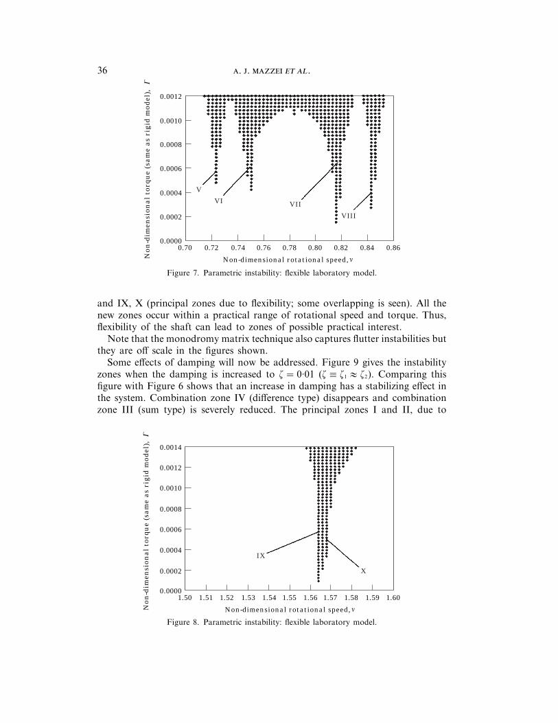
As a first example consider the laboratory model treated previously in section5. The natural frequencies corresponding to predominantly rigid modes for thissystem are nn1 =0·067 and nn2 =0·121. The first two natural frequencies associatedwith shaft flexibility for this system are nn3 =1·564 and nn4 =1·569. Figures 5 and

0.0012

0.0010

0.0008

0.0006

0.0004

0.0002

0.00000.08 0.10 0.12 0.140.060.040.020.00

Non-dimensional rotational speed,

No

n-d

imen

sio

na

l to

rqu

e (s

am

e a

s ri

gid

mo

del

),

IV

IIII

II

35

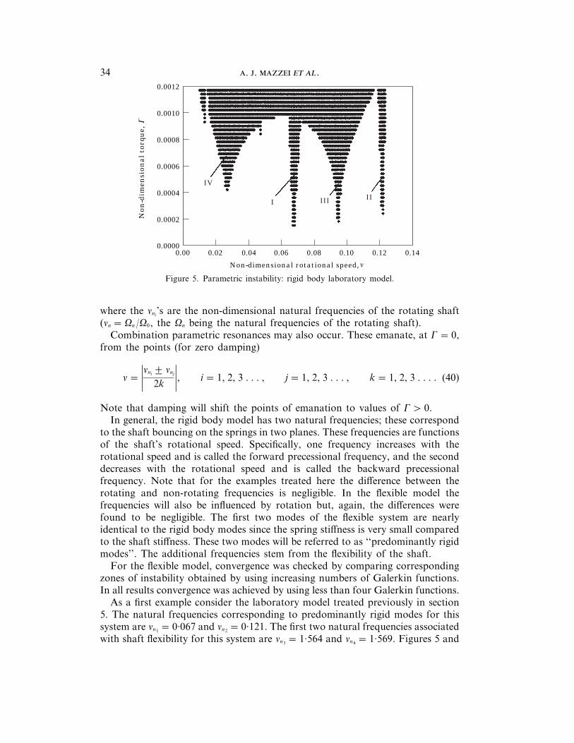
6 give plots of the instability zones (hashed zones indicate instability) as functionsof non-dimensional torque G and non-dimensional rotational speed n for the rigidbody model and for the flexible model, respectively (in Figure 6 the zones ofinstability corresponding to the shaft flexibility are off scale). In the figures, zonesI and II are principal zones emanating from nn1 =0·067 and nn2 =0·121,respectively, and zones III and IV are combination zones emanating from(nn1 + nn2)/2=0·094 (III) and (nn2 − nn1)/2=0·027 (IV). Note that the values of n

and G are within practical range. On the plots the rotational speeds range from,approximately, n=0·02 to 0·14 (54 to 376 rpm). The largest value of torque shownis G=0·0012 (0·84 Nm, which is approximately 29% of the value required foryielding).

It is seen that there is an excellent agreement between the zones predicted bythe two different models and so shaft flexibility does not influence the rigidinstability zones in this case. This is not surprising since the ‘‘rigid’’ frequenciesand ‘‘flexible’’ frequencies differ significantly. It is anticipated that flexibility willonly influence the ‘‘rigid’’ zones when the rigid and flexible natural frequencies areclose.

Note that the width of the zones is significant. For example, for a torqueG=0·0008 (19% of the yield torque) the shaft will cross four zones of instability.These are zone IV (about 47 rpm or 65% of the operating speed), zone I (about18 rpm or 10% of the operating speed), zone III (about 54 rpm or 21% of theoperating speed) and zone II (about 11 rpm or 3·4% of the operating speed). Notefurther that increasing the torque increases the width of the zones, thusdestabilizing the sytem.

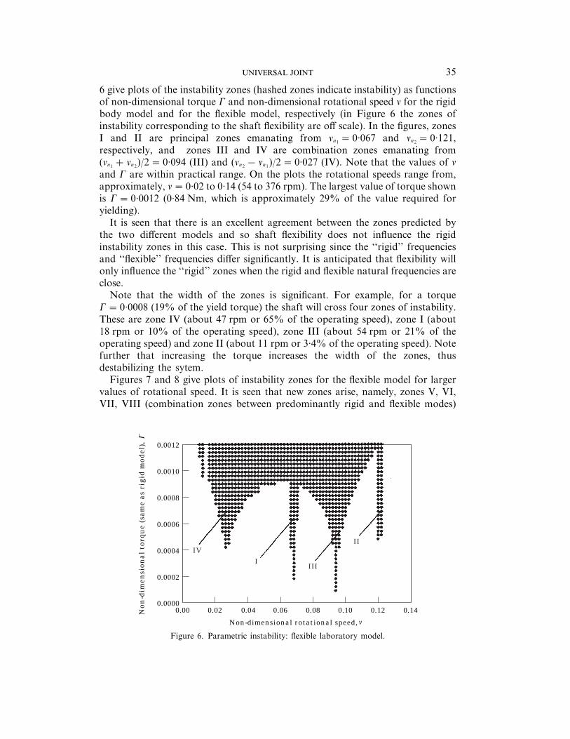
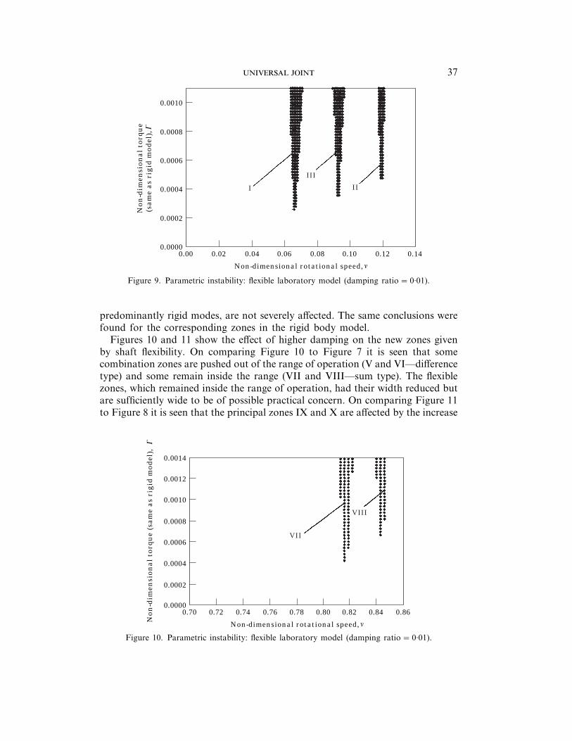
Figures 7 and 8 give plots of instability zones for the flexible model for largervalues of rotational speed. It is seen that new zones arise, namely, zones V, VI,VII, VIII (combination zones between predominantly rigid and flexible modes)

Figure 6. Parametric instability: flexible laboratory model.

0.0012

0.0010

0.0008

0.0006

0.0004

0.0002

0.00000.78 0.80 0.82 0.84 0.860.760.740.720.70

Non-dimensional rotational speed,No

n-d

imen

sio

na

l to

rqu

e (s

am

e a

s ri

gid

mo

del

),

V

VI VII

VIII

0.0014

0.0010

0.0012

0.0008

0.0006

0.0004

0.0002

0.00001.56 1.57 1.58 1.59 1.601.551.541.51 1.521.50

Non-dimensional rotational speed,No

n-d

imen

sio

na

l to

rqu

e (s

am

e a

s ri

gid

mo

del

),

1.53

IX

X

. . .36

Figure 7. Parametric instability: flexible laboratory model.

and IX, X (principal zones due to flexibility; some overlapping is seen). All thenew zones occur within a practical range of rotational speed and torque. Thus,flexibility of the shaft can lead to zones of possible practical interest.

Note that the monodromy matrix technique also captures flutter instabilities butthey are off scale in the figures shown.

Some effects of damping will now be addressed. Figure 9 gives the instabilityzones when the damping is increased to z=0·01 (z0 z1 1 z2). Comparing thisfigure with Figure 6 shows that an increase in damping has a stabilizing effect inthe system. Combination zone IV (difference type) disappears and combinationzone III (sum type) is severely reduced. The principal zones I and II, due to

Figure 8. Parametric instability: flexible laboratory model.

0.0008

0.0010

0.0006

0.0004

0.0002

0.00000.08 0.10 0.12 0.140.060.040.020.00

Non-dimensional rotational speed,

N

on

-dim

ensi

on

al

torq

ue

(sa

me

as

rig

id m

od

el),

III

III

0.0014

0.0010

0.0012

0.0008

0.0006

0.0004

0.0002

0.00000.80 0.82 0.84 0.860.780.760.72 0.740.70

Non-dimensional rotational speed,

No

n-d

imen

sio

na

l to

rqu

e (s

am

e a

s ri

gid

mo

del

),

VII

VIII

37

Figure 9. Parametric instability: flexible laboratory model (damping ratio=0·01).

predominantly rigid modes, are not severely affected. The same conclusions werefound for the corresponding zones in the rigid body model.

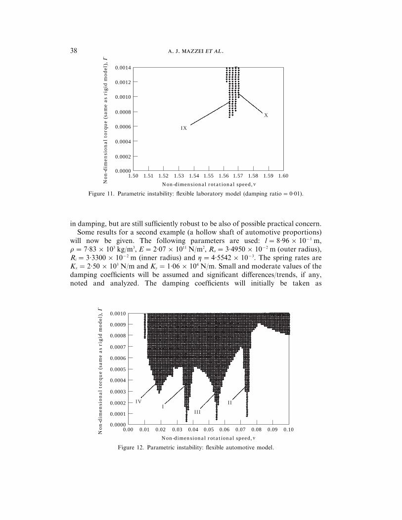
Figures 10 and 11 show the effect of higher damping on the new zones givenby shaft flexibility. On comparing Figure 10 to Figure 7 it is seen that somecombination zones are pushed out of the range of operation (V and VI—differencetype) and some remain inside the range (VII and VIII—sum type). The flexiblezones, which remained inside the range of operation, had their width reduced butare sufficiently wide to be of possible practical concern. On comparing Figure 11to Figure 8 it is seen that the principal zones IX and X are affected by the increase

Figure 10. Parametric instability: flexible laboratory model (damping ratio=0·01).

0.0014

0.0010

0.0012

0.0008

0.0006

0.0004

0.0002

0.00001.56 1.57 1.58 1.59 1.601.551.541.51 1.521.50

Non-dimensional rotational speed,No

n-d

imen

sio

na

l to

rqu

e (s

am

e a

s ri

gid

mo

del

),

1.53

IX

X

0.0010

0.0006

0.0007

0.0008

0.0009

0.0005

0.0004

0.0003

0.0001

0.0002

0.00000.06 0.07 0.08 0.09 0.100.050.040.01 0.020.00

Non-dimensional rotational speed,

No

n-d

imen

sio

na

l to

rqu

e (s

am

e a

s ri

gid

mo

del

),

0.03

IVI

III

II

. . .38

Figure 11. Parametric instability: flexible laboratory model (damping ratio=0·01).

in damping, but are still sufficiently robust to be also of possible practical concern.Some results for a second example (a hollow shaft of automotive proportions)

will now be given. The following parameters are used: l=8·96×10−1 m,r=7·83×103 kg/m3, E=2·07×1011 N/m2, Ro =3·4950×10−2 m (outer radius),Ri =3·3300×10−2 m (inner radius) and h=4·5542×10−3. The spring rates areKx =2·50×103 N/m and Ky =1·06×104 N/m. Small and moderate values of thedamping coefficients will be assumed and significant differences/trends, if any,noted and analyzed. The damping coefficients will initially be taken as

Figure 12. Parametric instability: flexible automotive model.

0.0011

0.0007

0.0009

0.0008

0.0010

0.0006

0.0005

0.0004

0.0003

0.0002

0.0001

0.00000.6 0.7 0.8 0.9 1.00.50.40.1 0.20.0

Non-dimensional rotational speed,

No

n-d

imen

sio

na

l to

rqu

e (s

am

e a

s ri

gid

mo

del

),

0.3

XI

VVI

39

Figure 13. Dynamic instability: flexible automotive model.

Cx =Cy =5·0×10−1 N/(m/s). The corresponding damping ratios are approxi-mately z1 =0·007 and z2 =0·003.

For this shaft static yielding will occur when the torque reaches approximately1·7×103 Nm (G=0·0005). The first four non-dimensional natural frequencies forthis system are: nn1 =0·036, nn2 =0·074 (predominantly rigid body modes),nn3 =1·563 and nn4 =1·565 (flexible modes).

Figure 12 shows the zones of parametric instabilities, given by the flexible model,for this system. Note the principal zones I (nn1) and II (nn2) and the combinationzones III ((nn1 + nn2)/2) and IV ((nn2 − nn1)/2). As in the laboratory model example,it is seen that the width of the zones can be of practical concern. For example,for rotational speeds ranging from 0 to 1500 rpm and for a level of torque around40% of the torque necessary to cause static yielding of the shaft (G=0·0002), thesystem will cross three zones of instability. These are: zone I (width of 101 rpm,roughly 18% of operating speed), zone III (width of 76 rpm, 9% of operatingspeed) and zone II (width of 25 rpm, 2% of operating speed).

Note also that, as in the previous example, an increase in torque leads to anincrease in the width of the zones (destabilizing effect on the system).

A comparison between Figure 12 and corresponding results using the rigid bodymodel revealed, as in the laboratory case, no significant differences.

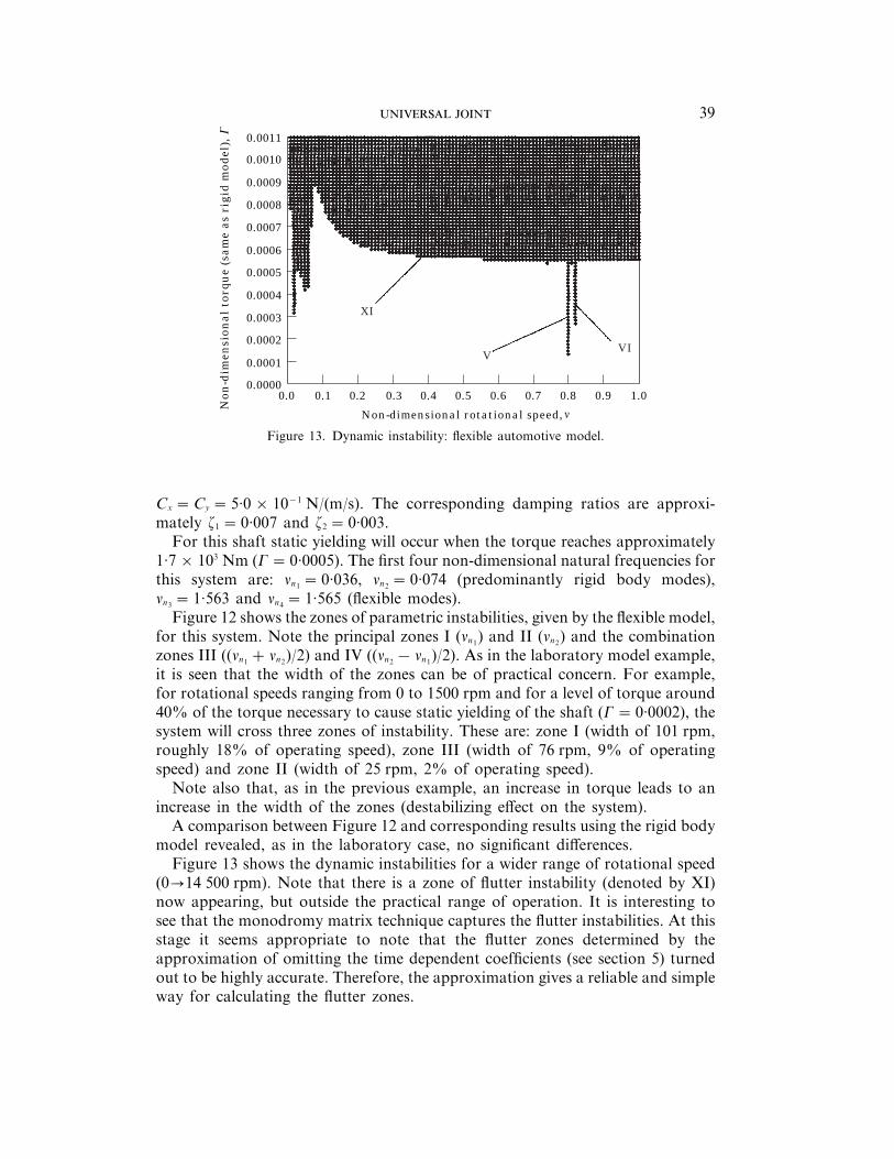
Figure 13 shows the dynamic instabilities for a wider range of rotational speed(0:14 500 rpm). Note that there is a zone of flutter instability (denoted by XI)now appearing, but outside the practical range of operation. It is interesting tosee that the monodromy matrix technique captures the flutter instabilities. At thisstage it seems appropriate to note that the flutter zones determined by theapproximation of omitting the time dependent coefficients (see section 5) turnedout to be highly accurate. Therefore, the approximation gives a reliable and simpleway for calculating the flutter zones.

0.0010

0.0007

0.0009

0.0008

0.0006

0.0005

0.0004

0.0003

0.0002

0.0001

0.00000.06 0.07 0.08 0.09 0.100.050.040.01 0.020.00

Non-dimensional rotational speed,

No

n-d

imen

sio

na

l to

rqu

e,

0.03

IV

I

III

II

Yield

. . .40

In addition to the predominantly rigid modes zones, Figure 13 shows twocombination zones between flexible and rigid modes, namely, zone V ((nn3 + nn1)/2)and zone VI ((nn4 + nn2)/2). In contrast to the laboratory model, here thesecombination zones are not of practical importance. The reason for that is the valueof the rotational speed for which they occur. These speeds are close to 11 650 rpm(n3 0·8) which is not practical for this system. Consequently, the parametricinstabilities of practical concern here are due to the predominantly rigid modesonly, in contrast to the laboratory model. Figure 13 does not include the instabilityzones due to flexibility since these occur at unreasonable values of rotational speed.Pure flexible zones are not important for the automotive shaft model, again incontrast to the laboratory model.

In summary the automotive shaft, either using the rigid body model or theflexible model, exhibits parametric instabilities under normal conditions ofoperation.

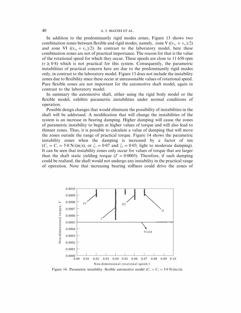
Possible design changes that would eliminate the possibility of instabilities in theshaft will be addressed. A modification that will change the instabilities of thesystem is an increase in bearing damping. Higher damping will cause the zonesof parametric instability to begin at higher values of torque and will also lead tothinner zones. Thus, it is possible to calculate a value of damping that will movethe zones outside the range of practical torque. Figure 14 shows the parametricinstability zones when the damping is increased by a factor of ten(Cx =Cy =5·0 N/(m/s), or z1 =0·07 and z2 =0·03; light to moderate damping).It can be seen that instability zones only occur for values of torque that are largerthan the shaft static yielding torque (G=0·0005). Therefore, if such dampingcould be realized, the shaft would not undergo any instability in the practical rangeof operation. Note that increasing bearing stiffness could drive the zones of

Figure 14. Parametric instability: flexible automotive model (Cx =Cy =5·0 N/(m/s)).

0.75

0.25

0.50

–0.50

–0.25

0.00

–0.751500 200010005000

Non-dimensional time,

Ga

mm

a (

rad

),

41

parametric instability outside the range of practical rotational speeds. However,the necessary increase in stiffness was found to be impractical.

7. NON-LINEAR MODEL

To conclude the work on instabilities of the homogeneous system, some resultsusing the non-linear rigid body model will now be presented. These results wereobtained using direct numerical integration of the equations of motion, subjectedto non-zero initial conditions. The laboratory model was employed in all cases.

One question that could be raised is whether the fact that flutter instabilitiesexist in the entire parameter space of n and G, for C=0, is due to the linearizationof the model. The answer was found to be no. The non-linear model, for theparameter values studied, also led to flutter instabilities everywhere for zerodamping.

Another issue is whether for C$ 0, the non-linear model would move the flutterinstability zones into regions of practical significance. The answer was found tobe no. Consider the example illustrated in Figure 3. Taking a point just inside andjust outside the boundary given there leads to the same conclusions as before.

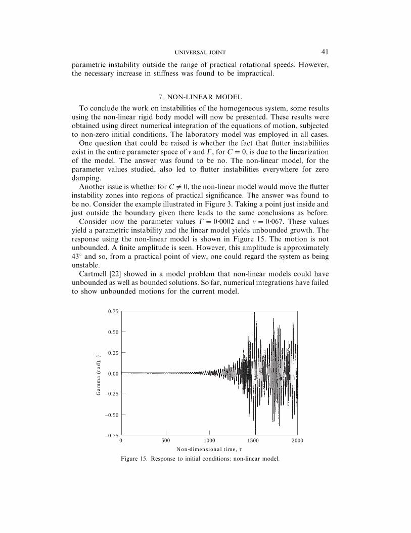
Consider now the parameter values G=0·0002 and n=0·067. These valuesyield a parametric instability and the linear model yields unbounded growth. Theresponse using the non-linear model is shown in Figure 15. The motion is notunbounded. A finite amplitude is seen. However, this amplitude is approximately43° and so, from a practical point of view, one could regard the system as beingunstable.

Cartmell [22] showed in a model problem that non-linear models could haveunbounded as well as bounded solutions. So far, numerical integrations have failedto show unbounded motions for the current model.

Figure 15. Response to initial conditions: non-linear model.

0.6

0.2

0.4

–0.4

–0.2

0.0

–0.64000 50002000 300010000

Non-dimensional time,

Bet

a (

rad

),

. . .42

For stable points the linear and non-linear models were found to be in excellentagreement.

8. FORCED MOTIONS

In this section forced instabilities of the systems described by equations (21)(rigid) and (31) (flexible) will be investigated.

Forced motions of ordinary differential equations with time dependentcoefficients have been studied extensively. See, for example, the recent work ofKang et al. [23]. Here a few observations will be made that are in no way meantto be exhaustive.

Of primary concern is whether new types of instability can occur. For example,Beale [24], using an extension of Hsu’s method [25], showed resonancescharacterized by linear growth were possible when the forcing frequency V isrelated to the natural frequencies Vn by

V=Vni

j, i=1, 2, 3 . . . , j=1, 2, 3 . . . .

For the current models, this condition translates, in dimensionless terms, to

n=nni

2j, i=1, 2, 3 . . . , j=1, 2, 3 . . . . (41)

No asymptotic solutions exist for the present models. Also the presence ofdamping makes the applicability of equation (41) to the present systemquestionable. Nonetheless, resonance points predicted by equation (41) wereexplored numerically for a few cases. The results were obtained using direct

Figure 16. Response of forced system: rigid body linear model (G=0·0002, n=0·0605—candi-date point for forced resonance).

0.6

0.2

0.4

–0.4

–0.2

0.0

–0.64000 50002000 300010000

Non-dimensional time,

Bet

a (

rad

),

2e–5

1e–5

–1e–5

0e+0

–2e–5400 500200 3001000

Non-dimensional time,

Bet

a (

rad

),

43

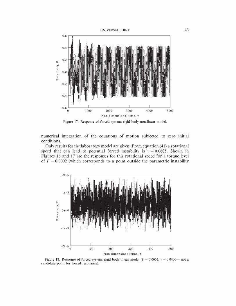
Figure 17. Response of forced system: rigid body non-linear model.

numerical integration of the equations of motion subjected to zero initialconditions.

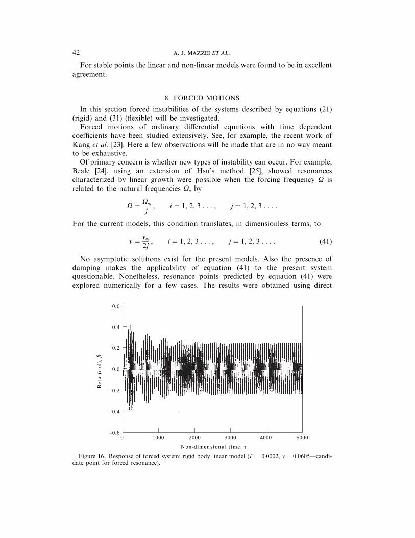
Only results for the laboratory model are given. From equation (41) a rotationalspeed that can lead to potential forced instability is n=0·0605. Shown inFigures 16 and 17 are the responses for this rotational speed for a torque levelof G=0·0002 (which corresponds to a point outside the parametric instability

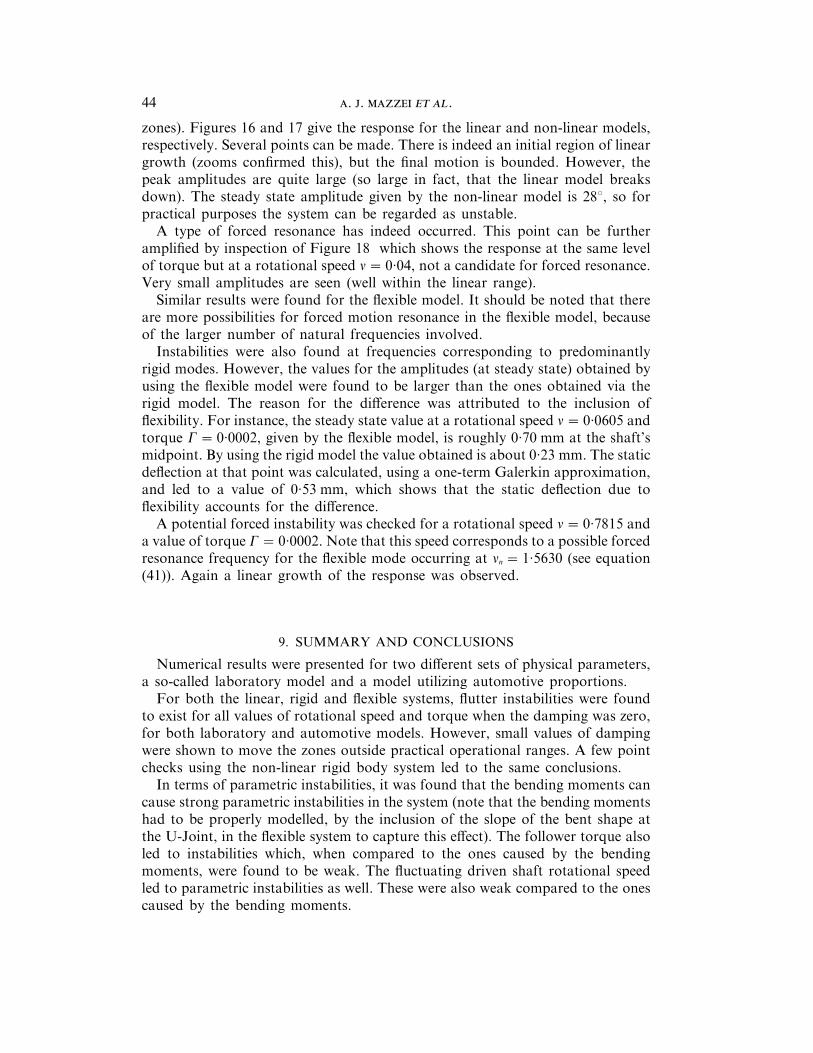
Figure 18. Response of forced system: rigid body linear model (G=0·0002, n=0·0400— not acandidate point for forced resonance).

. . .44

zones). Figures 16 and 17 give the response for the linear and non-linear models,respectively. Several points can be made. There is indeed an initial region of lineargrowth (zooms confirmed this), but the final motion is bounded. However, thepeak amplitudes are quite large (so large in fact, that the linear model breaksdown). The steady state amplitude given by the non-linear model is 28°, so forpractical purposes the system can be regarded as unstable.

A type of forced resonance has indeed occurred. This point can be furtheramplified by inspection of Figure 18 which shows the response at the same levelof torque but at a rotational speed n=0·04, not a candidate for forced resonance.Very small amplitudes are seen (well within the linear range).

Similar results were found for the flexible model. It should be noted that thereare more possibilities for forced motion resonance in the flexible model, becauseof the larger number of natural frequencies involved.

Instabilities were also found at frequencies corresponding to predominantlyrigid modes. However, the values for the amplitudes (at steady state) obtained byusing the flexible model were found to be larger than the ones obtained via therigid model. The reason for the difference was attributed to the inclusion offlexibility. For instance, the steady state value at a rotational speed n=0·0605 andtorque G=0·0002, given by the flexible model, is roughly 0·70 mm at the shaft’smidpoint. By using the rigid model the value obtained is about 0·23 mm. The staticdeflection at that point was calculated, using a one-term Galerkin approximation,and led to a value of 0·53 mm, which shows that the static deflection due toflexibility accounts for the difference.

A potential forced instability was checked for a rotational speed n=0·7815 anda value of torque G=0·0002. Note that this speed corresponds to a possible forcedresonance frequency for the flexible mode occurring at nn =1·5630 (see equation(41)). Again a linear growth of the response was observed.

9. SUMMARY AND CONCLUSIONS

Numerical results were presented for two different sets of physical parameters,a so-called laboratory model and a model utilizing automotive proportions.

For both the linear, rigid and flexible systems, flutter instabilities were foundto exist for all values of rotational speed and torque when the damping was zero,for both laboratory and automotive models. However, small values of dampingwere shown to move the zones outside practical operational ranges. A few pointchecks using the non-linear rigid body system led to the same conclusions.

In terms of parametric instabilities, it was found that the bending moments cancause strong parametric instabilities in the system (note that the bending momentshad to be properly modelled, by the inclusion of the slope of the bent shape atthe U-Joint, in the flexible system to capture this effect). The follower torque alsoled to instabilities which, when compared to the ones caused by the bendingmoments, were found to be weak. The fluctuating driven shaft rotational speedled to parametric instabilities as well. These were also weak compared to the onescaused by the bending moments.

45

Several types of parametric instability zones were found to exist in the models.These are zones of principal parametric instability, sum-type combination zonesand difference-type combination zones, involving rigid modes (the shaft bouncingon the bearing springs), flexible modes and combination of the predominantly rigidand flexible modes.

The parametric zones involving predominantly rigid modes were found to beof significant size and to occur at practical operating conditions in the laboratoryand automotive models. Parametric zones involving flexible modes (andcombination with predominantly rigid modes) were also found to occur in apractical range of operational conditions for the laboratory model. For theautomotive example, the zones due to flexibility and combination flexible–predom-inantly rigid modes occurred outside the range of operation. It should be notedthat the inclusion of flexibility in the modelling did not affect the parametric zonesdue to the predominantly rigid modes.

An increase in bearing damping will stabilize the system since the zones ofparametric instability occur for higher values of torque as the damping increases.For the laboratory model, an increase in damping more severely affected thedifference combination type zones of parametric instability. Sum-type zones andprincipal zones were also affected but to a lesser degree. A procedure was suggestedin order to reduce or eliminate the parametric instabilities. In the automotive casethe current models suggest that values of Cx =Cy =5·0 N/(m/s) for the dampingcoefficients would eliminate parametric instabilities from the practical range ofoperation. Whether such damping levels can be physically attained remains to beexplored.

In terms of forced instabilities, forced resonances were found to be possible, inboth models, when the rotational speed reached a value corresponding to anatural frequency of the system divided by two. Also, it was found thatflexibility was important in terms of the final steady state value for the forcedresponse of the driven shaft. In using the flexible model, the steady statevalues of the displacements are larger than the ones obtained by using the rigidmodel.

REFERENCES

1. H. P. L, T. H. T and S. B. L 1997 Journal of Sound and Vibration 199,401–415. Dynamic stability of spinning Timoshenko shafts with a time–dependent spinrate.

2. C. W. L and J. S. Y 1996 Journal of Sound and Vibration 192, 439–452. Dynamicanalysis of flexible rotors subjected to torque and force.

3. R. L. E and R. A. E 1969 ASME Journal of Engineering for Industry91, 1180–1188. On the critical speeds of a continuous rotor.

4. H. Z 1968 Principles of Structural Stability. Waltham, MA: Blaisdell PublishingCompany.

5. H. L 1987 Stability Theory—An introduction to the Stability of DynamicStystems and Rigid Bodies. New York: Wiley.

6. N. K 1997 Journal of Sound and Vibration 207, 287–299. Stability analysis forthe dynamic design of rotors.

. . .46

7. R. H. P and J. W 1995 Journal of Sound and Vibration 183, 889–897.Parametric, external and combination resonances in coupled flexural and torsionaloscillations of an unbalanced rotating shaft.

8. C.-W. L 1993 Vibration Analysis of Rotors. Boston, MA: Kluwer Academic Press.9. H. O and M. K 1984 Bulletin of JSME 27, 2002–2007. Lateral vibrations of a

rotating shaft driven by a universal joint—1st report.10. H. O, M. K and H. S 1985 Bulletin of JSME 28, 1749–1755. Lateral

vibrations of a rotating shaft driven by a universal joint—2nd report.11. M. K and H. O 1990 Journal of Vibration and Acoustics 112, 298–303. Lateral

excitation of a rotating shaft driven by a universal joint with friction.12. P.-P. S, W.-H. C and A.-C. L 1996 Journal of Vibration and Acoustics 118,

88–99. Modeling and analysis of the intermediate shaft between two universal joints.13. M. S, Y. O and K. O 1997 Journal of Vibration and Acoustics 119,

221–229. Self-excited vibration caused by internal friction in universal joints and itsstabilizing method.

14. S. F. A and M. C. H 1996 Journal of Vibration and Acoustics 118,368–374. Torsional instabilities in a system incorporating a Hooke’s joint.

15. S. F. A and X. H. W 1996 Journal of Sound and Vibration 194, 83–91.Characterization of torsional instabilities in a Hooke’s joint driven system via maximalLyapunov exponents.

16. R. M. R 1958 ASME Journal of Applied Mechanics 25, 47–51. On thedynamical behavior of rotating shafts driven by universal (Hooke) couplings.

17. T. I and M. S 1984 Journal of Sound and Vibration 95, 9–18. Transversevibration of a rotor system driven by a Cardan joint.

18. D. T. G 1988 Principles of Dynamics. Englewood Cliffs, NJ: Prentice–Hall.19. A. J. M, J. 1998 Doctoral Thesis, The University of Michigan, Ann Arbor.

Dynamic stability of a flexible spring mounted shaft driven through a universal joint.20. K. M. H, M. L. H and K. M. R 1996 Maple V—Learning Guide. New

York: Springer–Verlag.21. L. M 1970 Methods of Analytical Dynamics. New York: McGraw–Hill.22. M. C 1990 Introduction to Linear, Parametric and Nonlinear Vibrations. New

York: Chapman & Hall.23. Y. K, Y.-P. C and S.-C. J 1998 Journal of Sound and Vibration 209,

473–492. Strongly non-linear oscillations of winding machines, part I: mode-lockingmotion and routes to chaos.

24. D. G. B 1988 Doctoral Thesis, The University of Michigan, Ann Arbor. A studyof the motion of a flexible rod in a quick return mechanism.

25. C. S. H 1963 Journal of Applied Mechanics 30, 367–372. On parametric excitationof a dynamical system having multiple degrees of freedom.

26. M. D. G 1978 Foundations of Applied Mechanics. Englewood Cliffs, NJ:Prentice–Hall.

APPENDIX A: GALERKIN COEFFICIENTS

g1

0

d4Fm

dZ4 (Z)Fi (Z) dZ= a1mi , g1

0

d4Cm

dZ4 (Z)Ci (Z) dZ= a2mi ,

g1

0

Fm (Z)Fi (Z) dZ= g1mi , g1

0

Cm (Z)Ci (Z) dZ= g2mi ,

47

g1

0

Fm (Z)=Z=1Fi (Z)L(Z−1) dZ=Fm (Z)=Z=1Fi (Z)=Z=1 = j1mi ,

g1

0

Cm (Z)=Z=1Ci (Z)L(Z−1) dZ=Cm (Z)=Z=1Ci (Z)=Z=1 = j2mi ,

g1

0

dCm (Z)dZ bz=0

Fi (Z)dL(Z)

dZdZ=−

dCm (Z)dZ bz=0

dFi (Z)dZ bz=0

=−2d3mi ,

g1

0

dFm (Z)dZ bz=0

Ci (Z)dL(Z)

dZdZ=−

dFm (Z)dZ bz=0

dCi (Z)dZ bz=0

=−2d2mi ,

g1

0

dFm (Z)dZ bz=0

Fi (Z)dL(Z)

dZdZ=−

dFm (Z)dZ bz=0

dFi (Z)dZ bz=0

=−2d1mi ,

g1

0

dCm (Z)dZ bz=0

Ci (Z)dL(Z)

dZdZ=−

dCm (Z)dZ bz=0

dCi (Z)dZ bz=0

=−2d4mi ,

g1

0

d3Cm

dZ3 (Z)Fi (Z) dZ= b1mi , g1

0

d3Fm

dZ3 (Z)Ci (Z) dZ= b2mi ,

g1

0

d2Fm

dZ2 (Z)Fi (Z) dZ= l1mi , g1

0

d2Cm

dZ2 (Z)Ci (Z) dZ= l2mi ,

g1

0

d2Cm

dZ2 (Z)Fi (Z) dZ= l3mi , g1

0

d2Fm

dZ2 (Z)Ci (Z) dZ= l4mi ,

g1

0

Fm(Z)dL(Z)

dZdZ=−F'm (0), g

1

0

Cm (Z)dL(Z)

dZdZ=−C'm (0).

The following properties of the Dirac delta function were used [26] in derivingsome of the above results:

gb

a

D(Z− w)g(Z) dZ= g(w), gb

a

dD(Z− w)dZ

g(Z) dZ=−dg(Z)dZ bZ= w

,

aQ wQ b.