DYNAMIC RISK ANALYSIS OF OFFSHORE FACILITIES IN HARSH

ENVIRONMENTS

by

© Jinjie Fu

A thesis submitted to the

School of Graduate Studies

in partial fulfillment of the requirement for the degree of

Master of Engineering

Faculty of Engineering and Applied Science

Memorial University of Newfoundland

May 2020

St. John’s Newfoundland and Labrador

i

Abstract

With the frequent occurrence of extreme weather conditions, the safe operation of

offshore facilities has been seriously challenged. Previous research attempted to

simulate hydrodynamic performance or structure dynamic analysis to single

environmental load. The present thesis proposes two methodologies to assess the

operational risk quantitatively with combined wind and wave loads in a harsh

environment considering the dependence structure between the real-time

environmental parameters.

The first developed model calculates the environmental loads using wind load

response modeling, the Morison model and the ultimate limit states method. Then

physical reliability models and joint probability functions derive the probabilities

of failure at the level of structural components corresponding to combined loads.

BN integrates the root probabilities according to the unit configuration to calculate

the failure probability of the Semi-submersible Mobile Unit (SMU). The model is

examined with a case study of the Ocean Ranger capsizing accident on Feb 15,

1982. The model uses the prevailing weather conditions and calculates a very high

probability of failure 0.7812, which proves the robustness and effectiveness of the

proposed model.

The second proposed model is the copula-based bivariate operational failure

assessment function, which assesses the dependencies among the real-time

environmental parameters. Dependence function is described by the parameter δ

from the wave data and concurrent meteorological observation data which are

obtained from the Department of Fisheries and Oceans Canada (DFO). Then, the

true model is selected with the help of Akaike’s information criterion (AIC)

ii

differences and Akaike weight. Comparing the results from the proposed approach

and the traditional approach, it is shown that operational failure probabilities

considering dependence are noteworthy higher and deserve attention. In other

words, the traditional approach underestimates the operational risk of offshore

facilities, especially in harsh environments.

Keywords: Operational failure; Semi-submersible mobile unit; Physical reliability

model; Dependence; Copula function; Bayesian network; Environmental loads

iii

Acknowledgements

Studying at the Memorial University of Newfoundland with my supervisor Dr.

Faisal Khan is an unforgettable and wonderful period in my life. His excellent

attitude and rich academic background deeply impress me every time when we

discuss the research problems. In the academy, his meticulous attitude and high

standards urge me to keep forward. In life, he is more like a father, always

advising me on where my life should head to at the right time. I really appreciate

him for the patient guidance in the past two years of graduate study.

I also thankfully acknowledge the financial support from the Natural Science and

Engineering Council of Canada (NSERC) and the Canada Research Chair (CRC)

Tier I Program in Offshore Safety and Risk Engineering. I would like to thank

Chuanqi Guo and Guozheng Song, Ruochen Yang, and Xi Chen and all the

research fellows of Centre for Risk, Integrity, and Safety Engineering (C-RISE)

for their encouragement and constructive suggestions.

I am grateful to Daqian Zhang and Fan Zhang, Jin Gao and other friends, who

accompany and motivate me all the time in St. John’s. They make me feel that life

is colorful and full of sunshine. Last but not least, I am indebted to my beloved

parents for their love, constant support and encouragement. It is they who have

cheered me up and helped me through the hard times during the past twenty-four

years. Sureness, confidence, and kindness are the most important gifts they give

me. I dedicate this work to them.

iv

Table of Contents

Abstract ............................................................................................................................ i

Acknowledgements ........................................................................................................ iii

Table of Contents ........................................................................................................... iv

List of Tables .................................................................................................................. vi

List of Figures .............................................................................................................. viii

List of Abbreviations ....................................................................................................... x

Co-authorship Statement ............................................................................................... xii

Chapter 1. Introduction and Overview ................................................................. 1

Research on the evaluation impact of the environmental loads ........................... 1 1.1

Dynamic Risk Assessment ................................................................................... 3 1.2

Copula-based Dependency Analysis .................................................................... 6 1.3

Research objective of the thesis ........................................................................... 8 1.4

Thesis structure .................................................................................................... 9 1.5

References.......................................................................................................... 11 1.6

Chapter 2. Operational Failure Model for Semi-submersible Mobile

Units in Harsh Environments ........................................................................................ 17

Introduction........................................................................................................ 19 2.1

Methodology to Develop the Operational Failure Model .................................. 22 2.2

Identify relevant characteristics: physical and environmental ................... 23 2.2.1

Sections’ division and estimate components’ environmental loads ........... 25 2.2.2

Derive components’ probabilities of failure under combined loads .......... 27 2.2.3

Estimate the overall probability of failure using the BN ........................... 32 2.2.4

Testing of the model - the Ocean Ranger Disaster ............................................ 36 2.3

Identify SMU’s physical characteristics and weather condition ................ 37 2.3.1

Divide components’ sections and calculate corresponding environmental 2.3.2

loads 39

Derive components’ probabilities of failure under combined loads .......... 40 2.3.3

BN establishment and overall probabilities of failure estimation .............. 42 2.3.4

v

Results and Discussion ...................................................................................... 43 2.4

Conclusions........................................................................................................ 47 2.5

References.......................................................................................................... 49 2.6

Appendix ........................................................................................................... 53 2.7

Chapter 3. Monitoring and Modeling of Environmental Load

Considering Dependence and Its Impact on the Failure Probability ......................... 59

Introduction........................................................................................................ 61 3.1

The Proposed Methodology ............................................................................... 63 3.2

3.2.1 Step 1: Real-time weather observation....................................................... 65

3.2.2 Step 2: Environmental load calculation ..................................................... 65

3.2.3 Step 3: Define dependence calculated using data in Step 1 ...................... 67

3.2.4 Step 4: Failure probability calculation ....................................................... 72

3.2.5 Step 5: Compare and consider the maximum probability of failure .......... 74

Application of the proposed methodology ......................................................... 78 3.3

3.3.1 Steps 1-2: Real-time weather observation and environmental load

calculation ................................................................................................................. 78

3.3.2 Step 3: Define dependence calculated using data in Step 1 ....................... 80

3.3.3 Step 4-5: Failure probability calculation and comparison ......................... 82

Results and Discussion ...................................................................................... 84 3.4

Conclusions........................................................................................................ 88 3.5

References.......................................................................................................... 90 3.6

Chapter 4. Summary............................................................................................. 94

Conclusions........................................................................................................ 94 4.1

Recommendation ............................................................................................... 95 4.2

vi

List of Tables

Table 2-1 Main dimensions of the example SMU ................................................ 24

Table 2-2 Load calculation models ....................................................................... 26

Table 2-3 Nodes illustration in generic BN ........................................................... 34

Table 2-4 Physical characteristics of the Ocean Ranger (US Coast Guard, 1983) 37

Table 2-5 Nodes illustrations in Operational Failure Modeling of the Ocean

Ranger ................................................................................................................... 44

Table 2-6 The CPT of section #2, #3 and #4 for the derrick ................................. 53

Table 2-7 The CPT for the derrick ........................................................................ 53

Table 2-8 The CPT for the deck ............................................................................ 54

Table 2-9 The CPT of section #2, #3 and #4 for the corner column ..................... 54

Table 2-10 The CPT for the corner column .......................................................... 54

Table 2-11 The CPT for the supporting system..................................................... 55

Table 2-12 The CPT of section #2, #3 and #4 for the middle column .................. 55

Table 2-13 The CPT for the middle column ......................................................... 55

Table 2-14 The CPT for the chainlocker room and the ballast valves system ...... 56

Table 2-15 The CPT for the onboard liquid .......................................................... 56

Table 2-16 The CPT for the drilling water capacity and ballast water capacity ... 56

Table 2-17 The CPT for the fuel tank capacity and section #1 for the pontoon ... 56

Table 2-18 The CPT of section #2 for the pontoon ............................................... 57

Table 2-19 The CPT of section #3 and #4 for the pontoon ................................... 57

Table 2-20 The CPT for the pontoon .................................................................... 57

Table 2-21 The CPT for the pumping system ....................................................... 58

Table 2-22 The CPT for the Ocean Ranger ........................................................... 58

vii

Table 3-1 Physical characteristics of the sample object ........................................ 66

Table 3-2 CML and model selection calculation results ....................................... 71

Table 3-3 Environmental loads for the sample object ........................................... 74

Table 3-4 Failure probabilities using the example sample data ............................ 75

Table 3-5 Physical characteristics of the SMU ..................................................... 79

Table 3-6 CML and model selection calculation results for 1000 sets of data from

the buoy: Banquereau – 44139 .............................................................................. 81

Table 3-7 Environmental loads for the SMU ........................................................ 85

Table 3-8 Nodes probabilities of the Bayesian network ....................................... 86

viii

List of Figures

Figure 1-1. Flow diagram of the thesis structure .................................................. 10

Figure 2-1. Framework of operational failure modeling ....................................... 23

Figure 2-2. Schematic diagram for derrick (a), column (b) and pontoon (c) of the

example SMU with generated sections ................................................................. 25

Figure 2-3. (a) Random weather conditions and nodes' response; (b) Node's

physical maximum bearable corresponding wind speed/wave height .................. 29

Figure 2-4. Node's physical maximum bearable response corresponding Wind

speed/wave height ................................................................................................. 30

Figure 2-5. Generic BN of operational failure modeling ...................................... 34

Figure 2-6. Wind speed decay matching tendency model dependent on weather

data on the scene (US Coast Guard, 1983) ........................................................... 38

Figure 2-7. Schematic of the Ocean Ranger: derrick (a), middle and corner

column (b) and pontoon (c) with generated sections ............................................ 39

Figure 2-8. BN of operational failure modeling of the Ocean Ranger.................. 42

Figure 3-1. Real-time operational failure assessment methodology with copula-

based dependence .................................................................................................. 64

Figure 3-2. Scatter plot of the wind speed and wave height example................... 65

Figure 3-3. Schematic of the sample object with different sections ..................... 66

Figure 3-4. Scatter plot of wind speed and wave height after uniform

transformation ....................................................................................................... 70

Figure 3-5. Node's resistance response to environmental loads with different CVs

............................................................................................................................... 73

Figure 3-6. BN for the sample object .................................................................... 75

ix

Figure 3-7. Failure probability of section #2 (column) with dependent and

independent loads .................................................................................................. 77

Figure 3-8. Scatter plot of wind speed and wave height for Banquereau – 44139 78

Figure 3-9. Schematic of the typical SMU with generated sections ..................... 80

Figure 3-10. Scatter plot of wind speed and wave height after uniform

transformation for Banquereau – 44139 ............................................................... 81

Figure 3-11. Tailored BN for the SMU ................................................................. 83

Figure 3-12. Failure probabilities of section #1 and section #2 of the column with

dependent loads and independent loads ................................................................ 87

x

List of Abbreviations

ABS American Bureau of Shipping

AIC Akaike’s Information Criterion

BN Bayesian Network

BT Bow-tie

CBBN Copula-based Bayesian Network

CML Canonical Maximum Likelihood

COV/CV Coefficient of Variation

CPT Conditional Probability Table

DFO Department of Fisheries and Oceans

DRA Dynamic Risk Assessment

EML Exact Maximum Likelihood

ETA Event Tree Analysis

FSU Floating Storage Unit

FTA Fault Tree Analysis

IFM Inference Functions for Margins

IMS Improved Mixture Simulation

LLF Log-likelihood Function

MODU Mobile Offshore Drilling Unit

NOAA National Oceanic and Atmospheric

Administration

PDF Probability Density Function

PoF Probability of Failure

xi

QRA Quantitative Risk Assessment

SMU Semi-submersible Mobile Unit

TLP Tension Leg Platform

USNRC United State Nuclear Regulatory

Commission

xii

Co-authorship Statement

Jinjie Fu is the principal author of all the papers presented in the thesis. My

supervisor Dr. Faisal Khan identified the research gap and assisted Jinjie Fu to

determine the research topic. Then Jinjie Fu conducted an extensive literature

review and proposed related methodologies aiming to analysis operational risk in

terms of the combined environmental loads. Dr. Faisal Khan provided a solid

theoretical orientation in the research process. Furthermore, the calculation and

discussion of the results were finished by Jinjie Fu under the direct supervision of

Dr. Faisal Khan. Jinjie Fu prepared and revised the drafts of manuscripts based on

the suggestions of co-author Dr. Faisal Khan and the feedback from peer review.

1

Chapter 1. Introduction and Overview

As the source power of economic growth, energy plays a crucial role in national

living and industrial production, among which oil and natural gas occupy a

significant proportion. Offshore oil and gas reservoirs are increasingly attracting

people’s attention from conventional land-based reservoirs well drilling and

production to offshore hydrocarbon exploration and exploitation. However, it is

worth noting that the fickle and inclement ocean weather seriously threatens the

safe operation of the offshore facilities [1-2]. For instance, it reveals that the 2005

Atlantic hurricane season was the most active of record which includes the most

number of tropical storms (28) and the most number of hurricanes (15) according

to the annual summary from NOAA [3]. A tremendous amount of drilling and

production platforms were damaged or destroyed by hurricanes [4]. Therefore, the

rigorous situation underscores the urgent need for a suitable model to assess the

operational failure to guide and coordinate safety production.

Research on the evaluation impact of the environmental loads 1.1

To study the impact on the offshore facilities of the environmental loads, many

previous attempts have been conducted. Guan et al. [5] combined the finite

element method and wind field test to assess the derrick stress concentration of an

offshore module drilling rig under wind loads. Bea et al. [6] proposed an

integrated approach using the Morison model to calculate the wave impact loads

on the deck, validated by laboratory tests. Lee et al. [7] studied the derrick

performance considering gravity and wind pressure, based on the backpropagation

2

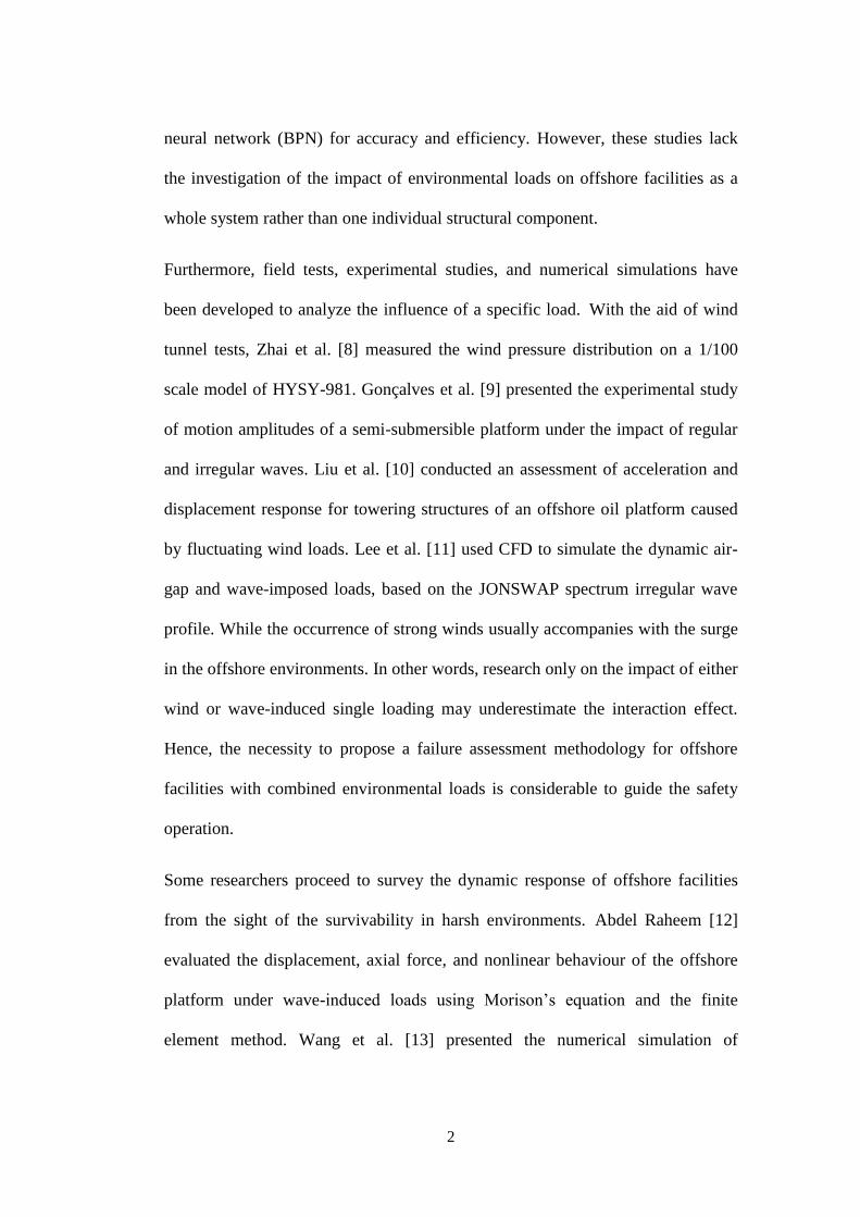
neural network (BPN) for accuracy and efficiency. However, these studies lack

the investigation of the impact of environmental loads on offshore facilities as a

whole system rather than one individual structural component.

Furthermore, field tests, experimental studies, and numerical simulations have

been developed to analyze the influence of a specific load. With the aid of wind

tunnel tests, Zhai et al. [8] measured the wind pressure distribution on a 1/100

scale model of HYSY-981. Gonçalves et al. [9] presented the experimental study

of motion amplitudes of a semi-submersible platform under the impact of regular

and irregular waves. Liu et al. [10] conducted an assessment of acceleration and

displacement response for towering structures of an offshore oil platform caused

by fluctuating wind loads. Lee et al. [11] used CFD to simulate the dynamic air-

gap and wave-imposed loads, based on the JONSWAP spectrum irregular wave

profile. While the occurrence of strong winds usually accompanies with the surge

in the offshore environments. In other words, research only on the impact of either

wind or wave-induced single loading may underestimate the interaction effect.

Hence, the necessity to propose a failure assessment methodology for offshore

facilities with combined environmental loads is considerable to guide the safety

operation.

Some researchers proceed to survey the dynamic response of offshore facilities

from the sight of the survivability in harsh environments. Abdel Raheem [12]

evaluated the displacement, axial force, and nonlinear behaviour of the offshore

platform under wave-induced loads using Morison’s equation and the finite

element method. Wang et al. [13] presented the numerical simulation of

3

hydrodynamic characteristics investigation of a semi-submersible platform with

nonsymmetrical pontoons under different wave directions. Zhu and Ou [14]

conducted a series of experiments to calculate the maximum horizontal

displacement of a semi-submersible platform with a mooring system. Using the

weather conditions of the South China Sea, Li et al. [15] discussed the motion

performance of the semi-submersible, tension leg platform (TLP), and Truss Spar.

These studies mainly focus on either the six-degree maximum motion behaviours

(pitch, yaw, sway, surge, heave and roll) or the stress, deformation and

acceleration response instead of ascertaining the anticipate operational risk

quantitatively. Therefore, this thesis proposes an integrated framework to assess

the operational risk quantitatively with combined wind and wave loads.

Dynamic Risk Assessment 1.2

To evaluate the operational risk of the offshore facilities, the risk assessment is the

most necessary part. As explained by Crowl and Louvar [16], the goal of the risk

assessment is to estimate the occurrence probabilities with the potential

consequences for accidents. Many researchers have proposed many related

methodologies that are successfully applied in the industrial circle. In general, two

main categories are able to represent the previous efforts: (1) Qualitative methods

and (2) Quantitative methods. The differences between the two above methods are

list as follows.

Method (1) is usually used as a screening process that tends to be applied to a

large group of process systems because it provides a relative risk result. In

contrast, method (2) is more comprehensive aiming at individual components or

4

technological processes and first developed by the USNRC (United States Nuclear

Regulatory Commission). Either deterministic or probabilistic results calculate the

risk for the target components or technological process with a concrete value.

Dynamic Risk Assessment (DRA) can guide the decision-making process for

systems due to its nature, the basis of which is the risk analysis approach. The

most popular and sophisticated approaches are the Bow-tie (BT) and the Bayesian

network (BN). BT consists of two sub approaches which are Fault Tree Analysis

(FTA) and Event Tree Analysis (ETA) according to the logic sequence. BT relies

on the ability to analyze the basic events which are the failures of the components

or operational process to form the intermediate events which further lead to the

top event. Then the various combination of the failure of safety barriers eventually

causes different accident scenarios. BT is widely applied in many fields [17-21]

because of the easily adopted feature and simplicity.

BT has the limitation to express the complex accident causation with traditional

logic gates, such as AND & OR gates, the applications of which are not enough to

be further expanded. Bayesian network (BN) receives researchers’ attention due to

the reason that conditional probability tables (CPT) solve the problems. BN is a

directed acyclic graphic model, which has the ability to use nodes and arcs to

represent variables and relationships among them along with the conditional

probability tables [22].

Khakzad et al. [23] illustrated the algorithm of how to map BT with BN with the

application of probability updating and probability adapting. BN is capable of

depicting the complex logic order of events and incorporating the probability of

failures (PoF) at the level of subsystems to the overall system. BN also has the

5

advantage of performing probability updating and adapting [23-24] because of the

unique characteristics for applying Bayes’ theorem in nature.

With the advantages, BN is applied by many scholars in different industrial fields,

especially in the offshore operation field. Bouejla et al. [25] developed a BN

which consisted of environmental limitations, threat characteristics and targets

under attack to assess the risks of piracy attacking offshore oil fields. Khakzad et

al. [26] used hierarchical Bayesian analysis to estimate the probability of failure

for offshore blowouts in the Gulf of Mexico, which can be applied to prevent

major accidents. Abimbola et al. [27] analyzed the high safety risk proposed by

MPD using BN with the intrinsic characteristics of dependencies modeling and

precursor data updating.

Many attempts have been made to apply other methods to improve BN. For

example, Guo et al. [24] proposed an innovative copula-based BN model that

developed joint non-linear relationships of process variables for decommissioning

process risk assessment. Khakzad et al. [28] employed an object-oriented BN risk

model considering time dependencies and physical parameters to quantify

offshore drilling operation risk.

In this thesis, the BN is applied and served as a robust tool to integrate the

probabilities of failure at the level of components’ sections calculated by the

physical reliability model to the level of components. Then, the failure probability

of the systems (offshore facilities) is estimated by incorporating the probabilities

of failure of essence structural components based on the units’ configuration. The

conditional probability tables stand for the mutual influence which reflects the

damage caused by the falling debris from the adjacent sections and components.

6

Copula-based Dependency Analysis 1.3

As mentioned in the previous section, researchers and engineers have applied

related standards to calculate environmental loads in order to study the dynamic

response or to better design the structural configuration of the offshore facilities.

These standards are usually recommended by some authoritative classification

societies, such as those used by DNV GL [29] and the American Bureau of

Shipping (ABS) [30]. For example, DNV GL standards were used by Suja-

Thauvin et al. [31] to compare the results of numerical simulation and the

experimental data of the monopile offshore wind turbine. To optimize design the

configuration of the 7th generation semi-submersible drilling unit (CSDU), Li et

al. [32] calculated hydrodynamic loads with the aid of the ABS rules.

However, it is obvious that the traditional approaches assess the operational safety

and risk for offshore facilities without considering the dependency among

parameters to calculate the environmental loads. In contrast, the harsh offshore

weather conditions may pose a risk to these facilities that are several higher than

expected. As a result, the occurrences of catastrophic accidents could be triggered

causing great loss and damage to crewmember lives, property, and environment.

Therefore, the research should be done to investigate the dependence structure to

prevent potential accidents to the greatest extent possible.

When it comes to dependence measurement, the Pearson linear correlation is the

most commonly used parameter because of the simple calculation procedure [33].

However, it needs to be clarified that the Pearson linear correlation parameter

7

follows the assumption of the corresponding elliptical multivariate distribution

[34]. It suits for examples like the bivariate normal distribution, which is far from

being as realistic as possible. More complex dependence structures call for a more

sophisticated approach.

Instead of relying on the linear correlation, copula functions address the limitation

to simulate complicated dependencies with the help of rank correlation. Kendall’s

tau and Spearman’s rho are two typical rank correlation parameters which are a

kind of concordance measure. Due to the natural scalar measure of the rank

correlation, monotonically transformations of the marginal random distributed

variables fail to change the dependencies. In other words, the scale-invariant

dependence measures of the rank correlation determine the marginal distribution-

free characteristic of the copula functions [35].

The most widely applied copulas are broadly divided into two main categories,

which are known as the explicit copulas and the implicit copulas [36]. The

implicit copulas are also called elliptical copulas which are derived from

multivariate distribution functions without closed-form integral solutions, such as

the Gaussian copula and the Student’s t-copula. However, the explicit copulas,

such as the Clayton copula, the Gumbel copula and the Frank copula which are

members of the Archimedian copula family, have simple closed forms that are

usually applied to low-dimensional systems [37].

Several available methods have been put forward to estimate the parameters of the

copula models. Manner [38] summarized five mature methods of the copula

parameter estimation which are known as the exact maximum likelihood (EML)

method, inference functions for margins (IFM) method, canonical maximum

8

likelihood method (CML) and two nonparametric estimation methods. The EML

and IFM are two parametric estimation methods while the CML is a

semiparametric estimation method.

Copula was first applied by economists to assess the financial risk because of its

ability to simulate complex tail dependencies. Manner [38] applied copulas to

simulate the exchange rate returns of Latin American currencies against the euro.

Melo et al. [39] used copulas to investigate the dependence behaviour of crude oil

and gasoline prices aiming to maximize the portfolio return. The copula gradually

comes into the application of the system safety and risk analysis with its potential

prevailing advantages. Pariyani et al. [40] applied the multivariate normal copula

and the Cuadras–Augé copula to study the interdependencies among the failure

probabilities of the safety, quality and operability systems. Hashemi et al. [37]

developed multivariate loss functions for process facilities operational loss

modeling that linked the marginal univariate loss functions with copula functions.

In this thesis, dependence functions among parameters to calculate the

environmental loads are described by the copulas.

Research objective of the thesis 1.4

The objective of this thesis is to analyze the operational risk of offshore facilities

in harsh environments. To be more specific, the research is implemented to fulfill

the following academic goals:

To assess the operational risk of the Semi-submersible Mobile Unit (SMU)

quantitatively with combined wind and wave loads in a harsh environment.

To investigate the influence of the dependence function among real-time

9

parameters to calculate environmental loads in terms of the impact on the

failure probability.

The first objective of this research is the development of the procedure to estimate

the anticipated operational risk of the SMU under combined loads. As mentioned

before, an operational risk calculation model overcomes the limitation of lacking

safety operation envelope reference for decision-makers. This procedure

associates related environmental loads calculation model and physical reliability

model which transfers the dynamic loads into probabilities of failure (POF). In

addition, the Bayesian network (BN) serves as a tool to integrate POF at the level

of the SMU.

The second objective of this thesis is the demystification of the effect of

dependence structure among real-time observed parameters to calculate the

environmental loads, which is a further extension of the first objective. As an

obvious fact that environmental parameters such as wind speed and wave heights

interact with each other. However, classification societies’ standards lack the

consideration of the non-linear dependencies. Therefore, in-situ wave and

concurrent meteorological observation data available online from the Department

of Fisheries and Oceans Canada (DFO) should be employed to simulate the loads

and impact on the failure probabilities of the system.

.

Thesis structure 1.5

This thesis is written in the manuscript format. It includes two peer-reviewed

journal manuscripts, one of which shown in Chapter 2 is accepted and published

on the Ocean Engineering journal and the other one presented in Chapter 3 is

10

submitted to the Ocean Engineering journal, as well. The outlines of the

aforementioned chapters are introduced as follows and shown in Figure 1-1.

Chapter 1 briefly introduces the previous research on the simulations of the

dynamic response of the offshore facilities and standards applications based on the

classification societies such as those used by DNV GL and the American Bureau

of Shipping (ABS). Furthermore, the latest applications of the BN and copula

models are covered in this chapter.

Figure 1-1. Flow diagram of the thesis structure

Chapter 2 includes a manuscript published in the Ocean Engineering journal in

2019. It proposes a methodology which recommends a rigorous procedure to

assess the anticipated operational risk of the SMU in harsh environments. With

the aid of DNVGL standards and physical reliability model, the probabilities of

failure at the level of structural sections are captured, which are further

incorporated by the BN. Then a well-known case application – the Ocean Ranger

11

confirms the effectiveness of the model, which helps to promote safe and reliable

offshore development.

Chapter 3 presents a manuscript submitted to the Ocean Engineering journal. A

robust copula-based bivariate operational failure assessment model which

considers the dependence functions among parameters to calculate the

environmental loads is proposed in this study. Wave and concurrent

meteorological observation data are accessed from the buoy: Banquereau – 44139

(available online from the Department of Fisheries and Oceans Canada (DFO)).

The comparison study of the proposed approach with the traditional approach

considering independence validates the robustness of the proposed risk analysis

model,

Chapter 5 summarizes the conclusions of the thesis and points several potential

research improvements and directions.

References 1.6

[1] Kaiser, M. J., & Yu, Y. (2010). The impact of Hurricanes Gustav and Ike on

offshore oil and gas production in the Gulf of Mexico. Applied

Energy, 87(1), 284-297.

[2] Cruz, A. M., & Krausmann, E. (2009). Hazardous-materials releases from

offshore oil and gas facilities and emergency response following

Hurricanes Katrina and Rita. Journal of Loss Prevention in the Process

Industries, 22(1), 59-65.

[3] Beven, J. L., Avila, L. A., Blake, E. S., Brown, D. P., Franklin, J. L., Knabb, R.

12

D., ... & Stewart, S. R. (2007). Annual summary: Atlantic hurricane season

of 2005. Monthly Weather Review, 136, 1109-1173.

[4] Cruz, A. M., & Krausmann, E. (2008). Damage to offshore oil and gas

facilities following hurricanes Katrina and Rita: An overview. Journal of

Loss Prevention in the Process Industries, 21(6), 620-626.

[5] Guan, F., Zhou, C., Wei, S., Wu, W., & Yi, X. (2014). Load-Carrying

Capacity Analysis on Derrick of Offshore Module Drilling Rig. Open

Petroleum Engineering Journal, 7, 29-40.

[6] Bea, R., Iversen, R., Xu, T., (2001). Wave-in-deck forces on offshore

platforms. Journal of offshore mechanics and arctic engineering, 123 (1),

10-21.

[7] Lee, J.-c., Jeong, J.-h., Wilson, P., Lee, S.-s., Lee, T.-k., Lee, J.-H., Shin, S.-c.,

(2018). A study on multi-objective optimal design of derrick structure:

Case study. International Journal of Naval Architecture and Ocean

Engineering, 10 (6), 661-669.

[8] Zhu, H., & Ou, J. (2011). Dynamic performance of a semi-submersible

platform subject to wind and waves. Journal of Ocean University of

China, 10(2), 127-134.

[9] Gonçalves, R. T., Rosetti, G. F., Fujarra, A. L., & Oliveira, A. C. (2013).

Experimental study on vortex-induced motions of a semi-submersible

platform with four square columns, Part II: Effects of surface waves,

external damping and draft condition. Ocean engineering, 62, 10-24.

[10] Liu, H., Chen, G., Lyu, T., Lin, H., Zhu, B., & Huang, A. (2016). Wind-

induced response of large offshore oil platform. Petroleum Exploration

13

and Development, 43(4), 708-716.

[11] Lee, S. K., Yu, K., & Huang, S. C. (2014). CFD study of air-gap and wave

impact load on semisubmersible under hurricane conditions. Paper

presented at the ASME 2014 33rd International Conference on Ocean,

Offshore and Arctic Engineering. San Francisco, USA

[12] Abdel Raheem, S. E. (2016). Nonlinear behaviour of steel fixed offshore

platform under environmental loads. Ships and Offshore Structures, 11(1),

1-15.

[13] Wang, S., Cao, Y., Fu, Q., & Li, H. (2015). Hydrodynamic performance of a

novel semi-submersible platform with nonsymmetrical pontoons. Ocean

Engineering, 110, 106-115.

[14] Zhu, H., & Ou, J. (2011). Dynamic performance of a semi-submersible

platform subject to wind and waves. Journal of Ocean University of

China, 10(2), 127-134.

[15] Li, B., Liu, K., Yan, G., & Ou, J. (2011). Hydrodynamic comparison of a

semi-submersible, TLP, and Spar: Numerical study in the South China Sea

environment. Journal of Marine Science and Application, 10(3), 306.

[16] Crowl, D. A., & Louvar, J. F. (2011). Chemical Process Safety-Fundamentals

with Applications. Process Safety Progress, 30(4), 408-409.

[17] Ferdous, R., Khan, F., Sadiq, R., Amyotte, P., & Veitch, B. (2013).

Analyzing system safety and risks under uncertainty using a bow-tie

diagram: An innovative approach. Process Safety and Environmental

Protection, 91(1-2), 1-18.

14

[18] Lu, L., Liang, W., Zhang, L., Zhang, H., Lu, Z., Shan, J., (2015). A

comprehensive risk evaluation method for natural gas pipelines by

combining a risk matrix with a bow-tie model. Journal of Natural Gas

Science and Engineering 25, 124-133.

[19] Abimbola, M., Khan, F., & Khakzad, N. (2014). Dynamic safety risk analysis

of offshore drilling. Journal of Loss Prevention in the Process Industries,

30, 74-85.

[20] Khakzad, N., Khan, F., & Amyotte, P. (2012). Dynamic risk analysis using

bow-tie approach. Reliability Engineering & System Safety, 104, 36-44.

[21] Yuan, Z., Khakzad, N., Khan, F., Amyotte, P., & Reniers, G. (2013). Risk-

based design of safety measures to prevent and mitigate dust explosion

hazards. Industrial & engineering chemistry research, 52(50), 18095-

18108.

[22] Yeo, C., Bhandari, J., Abbassi, R., Garaniya, V., Chai, S., Shomali, B.,

(2016). Dynamic risk analysis of offloading process in floating liquefied

natural gas (FLNG) platform using Bayesian Network. Journal of Loss

Prevention in the Process Industries 41, 259-269.

[23] Khakzad, N., Khan, F., & Amyotte, P. (2013). Dynamic safety analysis of

process systems by mapping bow-tie into Bayesian network. Process

Safety and Environmental Protection, 91(1-2), 46-53

[24] Guo, C., Khan, F., & Imtiaz, S. (2019). Copula-based Bayesian Network

Model for Process System Risk Assessment. Process Safety and

Environmental Protection.

15

[25]Bouejla, A., Chaze, X., Guarnieri, F., & Napoli, A. (2014). A Bayesian

network to manage risks of maritime piracy against offshore oil fields.

Safety science, 68, 222-230.

[26] Khakzad, N., Khakzad, S., & Khan, F. (2014). Probabilistic risk assessment

of major accidents: application to offshore blowouts in the Gulf of Mexico.

Natural Hazards, 74(3), 1759-1771.

[27] Abimbola, M., Khan, F., Khakzad, N., & Butt, S. (2015). Safety and risk

analysis of managed pressure drilling operation using Bayesian

network. Safety science, 76, 133-144.

[28] Khakzad, N., Khan, F., & Amyotte, P. (2013). Quantitative risk analysis of

offshore drilling operations: A Bayesian approach. Safety science, 57,

108-117.

[29] DNVGL-RP-C205, Enviromental conditions and enviromental loads. August

2017. DNV GL

[30] American Bureau of Shipping (ABS), Rules for building and Classing

Mobile Offshore Drilling Units. 2019

[31] Suja-Thauvin, L., Krokstad, J. R., & Bachynski, E. E. (2018). Critical

assessment of non-linear hydrodynamic load models for a fully flexible

monopile offshore wind turbine. Ocean Engineering, 164, 87-104.

[32] Li, D. J., Fu, Q., Du, Z. F., Xiao, Y., Han, R. G., & Sun, H. H. (2018).

Structural Configuration Selection and Optimization of 7th Generation

Semi-Submersible Drilling Unit. Paper presented at the ASME 2018 37th

International Conference on Ocean, Offshore and Arctic Engineering.

Madrid, Spain.

16

[33] Klaus, M. (2013) Multivariate Dependence Modeling using Copulas. Master

Thesis. Charles University in Prague.

[34] Hashemi, S. J., Ahmed, S., & Khan, F. I. (2015). Correlation and dependency

in multivariate process risk assessment. Paper Presented at the IFAC

SAFEPROCESS 2015: 9th IFAC Symposium on Fault

Detection, Supervision and Safety for Technical Processes, Paris, France.

[35] Nelsen, R.b., (2006). An introduction to Copulas, second ed. Springer, New

York, NY.

[36] Hashemi, S.J., (2016). Dynamic multivariate loss and risk assessment of

process facilities. Doctoral (PhD) thesis, Memorial University of

Newfoundland.

[37] Hashemi, S. J., Ahmed, S., & Khan, F. (2015). Operational loss modelling

for process facilities using multivariate loss functions. Chemical

Engineering Research and Design, 104, 333-345.

[38] Manner, H. (2007). Estimation and model selection of copulas with an

application to exchange rates. (METEOR Research Memorandum; No.

056). Maastricht: METEOR, Maastricht University School of Business

and Economics

[39] Melo, R., Accioly, S., & Aiube, F. A. L. (2008). Analysis of crude oil and

gasoline prices through copulas. Cadernos do IME-Série Estatística, 24(1),

15.

[40] Pariyani, A., Seider, W. D., Oktem, U. G., & Soroush, M. (2012). Dynamic

risk analysis using alarm databases to improve process safety and product

quality: Part II—Bayesian analysis. AIChE Journal, 58(3), 826-841.

17

Chapter 2. Operational Failure Model for Semi-submersible

Mobile Units in Harsh Environments1

Jinjie Fu and Faisal Khan*

Centre for Risk, Integrity and Safety Engineering (C-RISE),

Faculty of Engineering and Applied Science,

Memorial University of Newfoundland, St. John’s, NL, A1B 3X5, Canada

Abstract

The Semi-submersible Mobile Unit (SMU) plays a vital role in the development

of offshore oil and gas fields. Extreme weather conditions such as high winds,

waves, and icy conditions impose an extraordinary load on the platform. This

paper presents a detailed operational failure model considering the wind and wave

combined loading of extreme weather conditions. The model is developed in a

probabilistic framework using the Bayesian network (BN) to assess the

operational risk quantitatively. The BN represents conditional dependencies of the

weather effects and the operational characteristics of the SMU. The proposed

model is tested and validated using a well-known accident - the Ocean Ranger.

The model predicts a very high probability of operational failure (capsizing) in the

prevailing weather conditions, which is confirmed by the fateful event on Feb 15,

1982. The proposed model is a useful and reliable tool to develop and monitor the

1 Fu, J., & Khan, F. (2019). Operational failure model for semi-submersible mobile units in harsh

environments. Ocean Engineering, 191, 106332.

18

operational failure envelope of the SMU in given environmental conditions. This

work helps to promote safe and reliable offshore development.

Keywords: Operational failure; Bayesian network; Physical reliability model;

Semi-submersible unit; Wind and wave load; Offshore failure model

19

Introduction 2.1

With the acceleration of urbanization, land based oil exploitation alone cannot

meet people's growing demand for energy. Attention has therefore shifted to

offshore reservoirs, which contain tremendous oil and gas resources. However,

due to the complex and changeable marine environment, offshore drilling

accidents have occurred frequently in the last few decades. Through the analysis

of public records and reports, Ismail et al. (2014) stated that 15.1% of offshore

drilling accidents are caused by storms and hurricanes, second only to blowouts

over the last 56 years.

Previous research attempted to simulate the single environmental impact load on

the SMU. Ma et al. (2017b) developed a numerical simulation model to capture

the dynamic stress response of the derrick under random wind loads. Lee et al.

(2018) studied derrick performance, considering gravity and wind pressure.

Instead of taking the SMU as a whole system, only one or several structural

components have been analyzed. Note that all the elements working as a

harmonious integration interact with the complicated marine environment. Liu et

al. (2018) addressed performance-based analysis for the offshore jacket platform

subject to wind loads. Banks and Abdussamie (2017) developed wave and semi-

submersible interaction experiments using a piston-type wavemaker. However,

these models only analyzed the influence of a specific load with either wind or

wave-induced loading through numerical simulation, model experiments, or field

tests. Gomathinayagam et al. (2000) identified that wind load only accounts for 20%

- 25% of total loads in cyclonic winds. Especially during extreme weather

20

conditions, any components of the offshore structure may fail subject to wind and

wave combined impacts which potentially trigger a series of chain reactions.

Therefore, it is crucial to establish a damage assessment framework for the whole

SMU system which combines the predominant environmental loads, wind and

wave loads, simultaneously.

Research has been conducted to investigate the survivability of offshore platform

structure from external loading. Ma et al. (2017a) applied ANSYS and AQWA to

estimate structure and motion responses subjected to environmental loads. Ma et

al. (2019) put forward an Improved Mixture Simulation (IMS) method aiming to

describe stress responses and structural displacement of a semi-submersible

offshore platform. 3-D radiation and diffraction theory are employed to determine

the frequence and time response of a semi-submersible platform for the 100-year

return period of environmental loads (Ghafari and Dardel, 2018). Yu et al. (2018)

conducted hydrodynamic behaviour studies of TLP applying the JOHNSWAP

wave type. The aforementioned evaluation indicators pay more attention to either

external hydrodynamic performance or internal structure dynamic analysis rather

than assessing the operational risk quantitatively. Under the practical

circumstance, the operators want to ascertain the anticipate risk in the harsh

environments to guide the further decision. Consequently, how to evaluate the risk

posed by rogue waves and violent winds quantitatively appears to be particularly

important.

When it comes to employing risk analysis, quantitative risk assessment (QRA) is

a widely used effective technique. Especially in offshore operational fields

21

(Leimeister and Kolios, 2018) the Bayesian network (BN) is recommended for

risk assessment. As a graphic model, it uses nodes and arcs to represent variables

and relationships among them along with the conditional probability tables

(CPTs). The conditional dependencies are determined by either direct data or

subjective expert systems to reduce uncertainty(Yeo et al., 2016). Abaei et al.

(2018b) applied the BN to manage the risk arising from the storm of Floating

Storage Unit (FSU) based on the hydrodynamic accident load model. Barua et al.

(2016) mapped a dynamic fault tree into the Bayesian network to perform a

dynamic operational risk assessment with time-dependent characteristics. Song et

al. (2016) employed a BN model to investigate occupational risks for offshore

operations in harsh environments. Abaei et al. (2018a) integrated hydrodynamic

analysis and failure modeling using BN to assess the reliability of marine floating

structures. As a result, it can be concluded that BN is capable of estimating the

overall operational probability of failure of an offshore structure based on

conditional dependencies and subsystems’ failure probabilities in harsh

environments.

Accordingly, this work aims to propose a robust and reliable operational failure

model with the application of the BN for an SMU considering wave and wind

combined loads in a harsh environment. To begin with, environmental loads are

calculated with the help of wind load response modeling (DNVGL-RP-C205,

2017), the Morison model (DNVGL-RP-C205, 2017) and the ultimate limit states

method (DNVGL-RP-C103, 2015). Furthermore, structural components’

probabilities of failure are gathered thanks to different physical reliability models

and joint probability functions which combine the dynamic probabilistic response

22

to wind and wave loads. With the application of BN, the present study considers

the weather on site and the unit configuration to estimate the overall probability of

failure of an SMU, which provides an anticipated operational safety reference

value for decision making. This paper is organized as follows: Section 2.2

develops a methodology for operational failure modeling along with a simple case

example. The applicability is demonstrated with a case study in Section 2.3.

Section 2.4 briefly explains the impact of the operational state and the combined

loads, and Section 2.5 concludes the study.

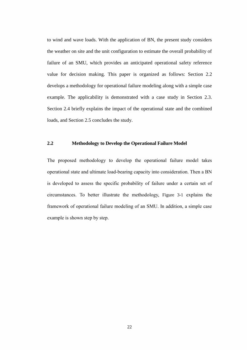
Methodology to Develop the Operational Failure Model 2.2

The proposed methodology to develop the operational failure model takes

operational state and ultimate load-bearing capacity into consideration. Then a BN

is developed to assess the specific probability of failure under a certain set of

circumstances. To better illustrate the methodology, Figure 3-1 explains the

framework of operational failure modeling of an SMU. In addition, a simple case

example is shown step by step.

23

Figure 2-1. Framework of operational failure modeling

Identify relevant characteristics: physical and environmental 2.2.1

The first step of the methodology is to identify the physical characteristics, which

include the fundamental configuration, operational state, and ultimate

environmental conditions. Subsequently, weather conditions on the scene should

be clarified through related weather forecasts. A simplified case is used to

demonstrate the operational risk assessment model for the SMU. Table 2-1 shows

24

the geometric dimensions of the example SMU. For the sake of simplicity, the aim

is to assess the operational probability of failure under the harsh weather

conditions of 80 knots wind speed and 70 ft wave height. Holmes (2015)

developed the power law profile to describe the wind speed above the ground. The

profile used a reference mean wind speed for 10 minutes at 10 m height above

ground.

(𝑧)𝑈− = (𝐻)(

𝑧

𝐻)𝑧0

𝑈− ( 2.1 )

where z is the height, (H)U− is the reference mean wind speed for 10 minutes, H is

the reference height equal to 10m and z0 is the terrain roughness parameter.

Table 2-1 Main dimensions of the example SMU

Component Dimension Component Dimension

Length of pontoons 200 ft Upper deck 150 ft

Height of pontoons 20 ft Lower deck 120 ft

Width of pontoons 20 ft Operational draft 80 ft

Diameter of columns 30 ft Height of derrick 160 ft

Height of columns 100 ft Affordable wind speed 100 knots

Number of columns 4 Affordable wave height 100 ft

Wave fluid particle speed and acceleration are derived from the derivative of the

wave velocity potential concerning displacement and then time, respectively. The

formulae involved for fluid particle velocity and acceleration of the corresponding

second-order Stokes wave theory are provided in DNVGL-RP-C205 (2017).

25

Sections’ division and estimate components’ environmental loads 2.2.2

According to the offshore structure design standard (DNVGL-OS-C201 2017;

DNVGL-OS-C101 2019; DNVGL-OS-C201, 2017), it is essential to take

environmental loads, wind and hydrodynamic loads induced by waves into

consideration for mobile offshore units operating under harsh environmental

conditions.

Figure 2-2. Schematic diagram for derrick (a), column (b) and pontoon (c) of the

example SMU with generated sections

The SMU is a widely deployed engineering equipment for offshore deep-water oil

26

and gas development, which mainly consists of a derrick, deck, columns, and

pontoons. In order to better assess the response of structural components’

probabilities of failure in detail, the main components of the unit, consisting of the

derrick, pontoons, and columns, are divided into four generated sections (from

section #1 to #4) as indicated in Figure 2-2. Every section includes many nodes

which are statistically finite. To be noticed, these sections are also developed to

form root nodes of the BN. As a result, wind and wave characteristics are

determined through a wind speed profile and second-order Stokes wave theory.

Accordingly, Table 2-2 presents wind, wave load, and sea pressure, which are

calculated for sections through wind load response modeling, the Morison model

and the ultimate limit states method.

Table 2-2 Load calculation models

Load Model

Wind load Wind load response modeling (DNVGL-RP-C205, 2017)

Wave load Morison model (DNVGL-RP-C205, 2017)

Sea pressure Ultimate limit states method (DNVGL-RP-C103, 2015)

Although the vertical wave loads sometimes exceed horizontal wave loads for the

SMU, buoyancy force and gravitational force partially counteract the effects of

the waves’ force. Additionally, the deck is usually designed as grated and open

(non-plated) to reduce all kinds of contamination in the deck area, and to avoid

slip/fall accidents. Bea et al. (2001) insisted that vertical force is negligible

compared to horizontal force on open, grated decks. Technically, the crux of the

27

proposed methodology is to capture the probability of failure by incorporating the

ultimate load and operational load, regardless of the direction, into the physical

reliability model. Hence, only the horizontal wave load and sea pressure are

discussed in this paper. The permissible loads and actual loads on the basis of real

weather on the scene are presented in Table 2-3.

Derive components’ probabilities of failure under combined loads 2.2.3

The physical reliability model assumed that reliability is independent of the time

parameter (Khakzad et al., 2012). In this model, the relationship between stress

and strength is analyzed through a given distribution of the variables. The

probability of failure can be quantified by integrating the stress or strength

distribution. Intuitively, the loads are randomly distributed because of random

weather conditions in nature, as reflected in part (a) of Figure 2-3. However, every

section presented in Figure 2-2 includes many nodes, which are statistically finite,

as mentioned. Every black line in part (a) of Figure 2-3 represents various nodes’

resistance to loads, which involve their specific responses owing to stress

concentration, unit configuration, and so on, to different loads. For a particular

node, there exists a unique probabilistic response for dynamic external loads.

Then, it is assumed that the dynamic probabilistic response of all nodes in an

individual section follows lognormal distribution, for mathematical convenience,

with location parameter 𝑡𝑚𝑒𝑑 and shape parameter as shown in part (b) in Figure

2-3. The x-coordinate represents the corresponding maximum bearable weather

response index such as wind speed or wave height, for all nodes in a certain

28

section, instead of the physical properties of materials.

𝑃(𝑅 < 𝐿) = ∫ 𝑓𝑟(𝑟)𝐿

0𝑑𝑟 = 𝛷(

1

𝑠𝑙𝑛

𝐿

𝑡𝑚𝑒𝑑) ( 2.2 )

The next step is to determine the shape parameter and location parameter in

Equation (2.2). It is worth mentioning that both parameters can be related to mean

µ and standard deviation σ through mathematical transformation. A reasonable

coefficient of variation (COV) helps to solve them. In the work of Cheng and

Yeung (2002), there is nearly 99% certainty that the COV is between 0.05 and

0.20 based on the available wind speed statistical data in 143 weather stations in

the United States. Because the marine environment of the SMU is relatively harsh,

the COV should be adjusted appropriately to between 0.01 and 0.5. Generally

speaking, COV stands for the degree of data concentration and dispersion as

shown in Figure 2-4. Compared to the red case, the blue case has a higher COV,

which is quite more even and scattered. With the environmental loads producing

small variations, the resistance response of the blue case tends to change

dramatically due to stronger sensitivity generated by a greater COV. In an

interview (Zhang, 2017), Robert Bea, a professor emeritus in civil engineering at

the University of California, Berkeley said “The pressures generated in those

wave crests can exceed several thousand pounds per square inch,”. He argues that

“Offshore platforms can generally deal with wind and rainfall okay, but cresting

waves will do real damage.” Therefore, it is assumed that COV is 0.074 for every

section’s statistically distributed wind resistance response and 0.1 for statistically

distributed wave resistance response for the example SMU.

DNVGL-OS-C101 (2019) suggested that the probability of exceedance for wind

and wave induced loads should be no more than 10−2 under the maximum design

29

loads. Once the ultimate load-bearing capacity for each section (loads produced

by 100 knots wind speed and 100 ft wave height in the example, respectively) is

calculated with load calculation models, L and P are substituted into Equation

(2.2) with above loads separately (the first step is to obtain the probability of

failure under single load impact) and10−2 . By combinations of simultaneous

COV equations, shape and location parameters can be solved to determine the

probability of failure under any weather conditions on the scene for non-specific

sections against a single load.

Figure 2-3. (a) Random weather conditions and nodes' response; (b) Node's

physical maximum bearable corresponding wind speed/wave height

30

Figure 2-4. Node's physical maximum bearable response corresponding Wind

speed/wave height

It is known that the SMU has to deal with multivariate site-specific environmental

loads in a harsh environment. For example, wind and wave induced loads affect

deck and columns above the draft. Additionally, pontoons and columns below the

draft suffer the damage of sea pressure and wave induced loads. In spite of the

fact that the probabilistic response for a non-specific section against a single load

is solved, sections’ different probabilistic responses regarding the different loads

need to be combined. In this paper, the sections’ response for wind and wave loads

are treated differently rather than using simple mathematical addition. As a

consequence, a joint probability distribution can be applied to assess the

components’ probability of failure.

Joint probability functions (Forbes et al., 2011) are known as multivariate

distributions, which can describe the distribution of multiple random variances

concerning regions of N-dimensional space. Moreover, the probability of a set of

31

random variables can be obtained through marginalization. A bivariate lognormal

distribution is adapted, owing to the fact that not only are there positive values for

loads without a clear increasing tendency, but also because the marginal

probability distribution follows a lognormal distribution. The probability density

function (PDF) of joint and marginal distributions of random variables X and Y is:

𝑓(𝑥, 𝑦) =1

2𝜋𝜎𝑥𝜎𝑦𝑥𝑦√1−𝜌2exp {−

1

2(1−𝜌2)[(

𝑙𝑛𝑥−𝜇𝑥

𝜎𝑥)

2− 2𝜌 (

𝑙𝑛𝑥−𝜇𝑥

𝜎𝑥) (

𝑙𝑛𝑦−𝜇𝑦

𝜎𝑦) + (

𝑙𝑛𝑦−𝜇𝑦

𝜎𝑦)

2

]}

(𝑥 > 0, 𝑦 > 0, −1 < 𝜌 < 1) ( 2.3 )

𝑓(𝑥) =1

√2𝜋𝜎𝑥𝑥𝑒𝑥𝑝 (−

1

2𝜎𝑥2 (𝑙𝑛

𝑥

𝑒𝜇𝑥)2) , (𝑥 > 0) ( 2.4 )

𝑓(𝑦) =1

√2𝜋𝜎𝑦𝑦𝑒𝑥𝑝 (−

1

2𝜎𝑥2 (𝑙𝑛

𝑦

𝑒𝜇𝑦)2), (𝑦 > 0) ( 2.5 )

where ρ is the correlation coefficient, 𝜎𝑥 , 𝜎𝑦 are the standard deviation and 𝜇𝑥 ,

𝜇𝑦 are the mean of ln 𝑋, ln 𝑌.

To conclude, operationally safe wind and wave loads can be calculated using the

design with affordable wind speed and wave height as provided in the SMU safe

operation manual, respectively. Then, the annual probability of exceedance is

10−2 for the operational safety wind and wave loads, as stipulated by DNVGL-

OS-C101 (2019). In addition, marginal probability distribution parameters for

every section under a single designed and manufactured maximum load response

are calculated combining the assumed simultaneous COV equations. Ultimately,

the joint bivariate lognormal distribution is applied to determine the probability of

failure for every analytical section under combined loads (X = wind loads and Y =

wave loads at sections level). Parameters of the joint bivariate lognormal

distribution are from the marginal distributions which are the components’

32

response to a single load. In this paper, it is assumed that wind load and wave load

are independent of each other. Consequently, the correlation coefficient ρ in the

joint probability functions equals 0. Under these conditions, the probabilities of

failure at components’ levels under combined wind and wave induced loading are

completed.

During the monitor period in operation, the maximum wind speed and wave

height can be observed which are used to gain real time environmental load. Then

the loads are substituted into the solved bivariate log-normal distribution to assess

the real time operational risk. Table 2-3 summarizes the probabilities of failure for

each section of the principal components. Next step is to estimate the overall

probability of failure with the aid of the BN.

Estimate the overall probability of failure using the BN 2.2.4

A BN is a directed acyclic graphical model (Weber et al., 2012), which is

composed of random variables that represent root causes, arcs that clarify

dependencies between parent nodes and child nodes, and the conditional

probability that quantifies forward predictive inference.

𝑃(𝐴) = ∑ 𝑃(𝐴|𝐵𝑖)𝑃(𝐵𝑖)𝑛𝑖=1 ( 2.6 )

where 𝑃(𝐴|𝐵𝑖) is conditional probability and 𝑃(𝐵𝑖) is the probability of the ith

variable.

Conditional probability tables (CPT) of BNs are achieved according to the

weights of events, which come from the survey with prior probabilities of primary

events or subjective belief. The weight of an event refers to the likelihood of

33

occurrence of its upper events, given the event’s occurrence. In this paper,

subjective opinions satisfy the primary purpose of assessing the probabilities of

operational failure in a harsh environment. The sixth generation of the deep water

SMU mainly consists of a derrick, deck, columns, and pontoons. The deck houses

all drilling machinery, including the derrick, material storage, and living facilities.

Columns are located between the deck and pontoons, supporting the unit with four

to eight vertical cylinders. Pontoons composed of oil tanks, ballast water tanks

and drill water tanks provide flotation to the system. In the demonstration

example, only corner columns are considered. Figure 2-5 illustrates the general

BN assessing the probability of failure of an example SMU. The root nodes are

from the sections of each structural component. DS 1 - 4 represent sections #1 to

#4 of the derrick. Similarly, CS 1 – 4 and PS 1 - 4 represent sections #1 to #4 of

the corner columns and pontoons, as illustrated in Figure 2-2.

In order to distinguish the damage caused by the section itself (response to

environmental loads) and the adjacent section, the suffix ‘S’ is applied. For

example, DS3 indicates the damage caused by environmental loads to section #3

of the derrick directly and DS3S expresses the damage caused by both

environmental loads directly and collateral debris from section #2 of the derrick.

Because of the unit configuration, it is assumed that only two adjacent sections

interact with the debris trajectory. In short, the greater the height of the section,

the greater the mutual influence factor is, since the uppermost section has the

strongest potential of both kinetic and gravitational failure. In this paper, failure of

any component (derrick, deck, column and pontoon) triggers the damage to the

overall platform. Finally, BN combines all the structural components to estimate

34

the overall probability of failure (PoF) under the weather on the scene to create a

general assessing framework. The results of the operational probabilities of failure

for components and the platform are presented in Table 2-3.

Figure 2-5. Generic BN of operational failure modeling

Table 2-3 Nodes illustration in generic BN

Permissible Load Actual Load

PoF Component Wind

103 Pa

Wave

104 Pa

Sea pressure

105 Pa

Wind

103 Pa

Wave

104 Pa

Sea pressure

105 Pa

Derrick - - - - - - 4.00×10-4

Section #1 3.42 - - 2.19 - - 1.07 ×10-4

35

Section #2 3.25 - - 2.08 - - 1.04×10-4

Section #3 3.04 - - 1.95 - - 1.17 ×10-4

Section #4 2.79 - - 1.78 - - 8.79×10-5

Deck 2.47 7.60 - 1.58 3.23 - 1.64×10-5

Columns - - - - - - 7.07×10-5

Section #1 2.14 3.43 - 1.37 2.41 - 1.23×10-5

Section #2 1.57 3.05 - 1.00 2.17 - 1.15×10-5

Section #3 - 2.65 4.16 - 1.90 3.82 2.91×10-8

Section #4 - 2.25 5.13 - 1.62 4.8 4.69×10-5

Pontoons - - - - - - 7.00×10-5

Section #1 - 1.52 5.95 - 1.05 5.61 1.60×10-5

Section #2 - 1.52 5.95 - 1.05 5.61 1.60×10-5

Section #3 - 1.52 5.95 - 1.05 5.61 1.60×10-5

Section #4 - 1.52 5.95 - 1.05 5.61 1.60×10-5

SMU - - - - - - 6.00×10-4

The simulation results in Table 2-3 show that the platform will bear a tolerable

probability of failure if it operates under 80 knots of wind and a 70 ft wave height

simultaneously. Generally, in accordance with DNVGL-OS-C101 (2019), the

operational failure envelope of in situ operational probability of failure can be

defined as [10-2

, 1]. The explanation for the operational failure envelope is that the

higher the failure probability of the system, the greater the destructive potential.

Once the result of operational failure modeling based on weather data on the scene

is calculated, further recommendations are suggested to avoid catastrophic

disaster. If the estimated probability of failure falls in the operational failure

envelope, it is recommended to terminate the operation and drag the SMU back to

36

the harbour to reduce risk. In contrast, it is allowed to continue operating if the

proper procedure is followed and real-time conditions are monitored in case of

rapidly changing weather conditions. As an anticipated risk estimation model, the

proposed operational failure model is capable of capturing real-time weather data

on the scene and the current operational state to provide a safety operational

perspective.

Testing of the model - the Ocean Ranger Disaster 2.3

To verify the proposed methodology, a case study was conducted. The aim of the

case study was to model the prevailing conditions during the Ocean Ranger oil rig

disaster. The accident occurred off the coast of Newfoundland on Feb 15, 1982.

Heising and Grenzebach (1989) earlier studied this accident using a fault tree with

a beta factor to assess the capsize probability of the Ocean Ranger. Several core

components, including pumps, valves, and onboard liquids, were utilized to

analyze the failure probability using common cause failure. According to the

Marine Casualty Report - Mobile Offshore Drilling Unit (MODU) Ocean Ranger

(US Coast Guard, 1983), rogue waves which were still in the acceptable height

range attacked the Ocean Ranger. Due to the design flaw, the ballast control room

with the open deadlight was located close to the drilling draft water line. As a

result, the rig capsized and sank in the Grand Banks area, 267 kilometers east of

St. John’s, Newfoundland (US Coast Guard, 1983).

37

Identify SMU’s physical characteristics and weather condition 2.3.1

To begin, Table 2-4 illustrates the geometric scale parameters of the Ocean

Ranger. According to the final report by the US Coast Guard (1983), the Ocean

Ranger was able to withstand 100-knot winds and 110-ft waves at the same time.

Subsequently, the wind speed predictive development model is the basis of the

entire risk assessment process, owing to the fact that both the wind’s inflicted

destruction potential and wind-induced wave damage are dominated by wind

speed. Thus, a simple empirical database derived hurricane wind model is adapted

for predicting the maximum wind of tropical cyclones (Kaplan and DeMaria,

1995).

Table 2-4 Physical characteristics of the Ocean Ranger (US Coast Guard, 1983)

Component Dimension Component Dimension

Length of pontoons 398.6 ft Drilling draft 80 ft

Height of pontoons 24 ft Height of derrick 185.4 ft

Width of pontoons 62 ft Diameter of corner columns 36 ft

Upper deck 151.6 ft Diameter of middle columns 25 ft

Lower deck 134 ft Height of ballast control room 108 ft

Height of columns 110 ft Affordable wind speed 100 knots

Number of columns 8 Affordable wave height 110 ft

38

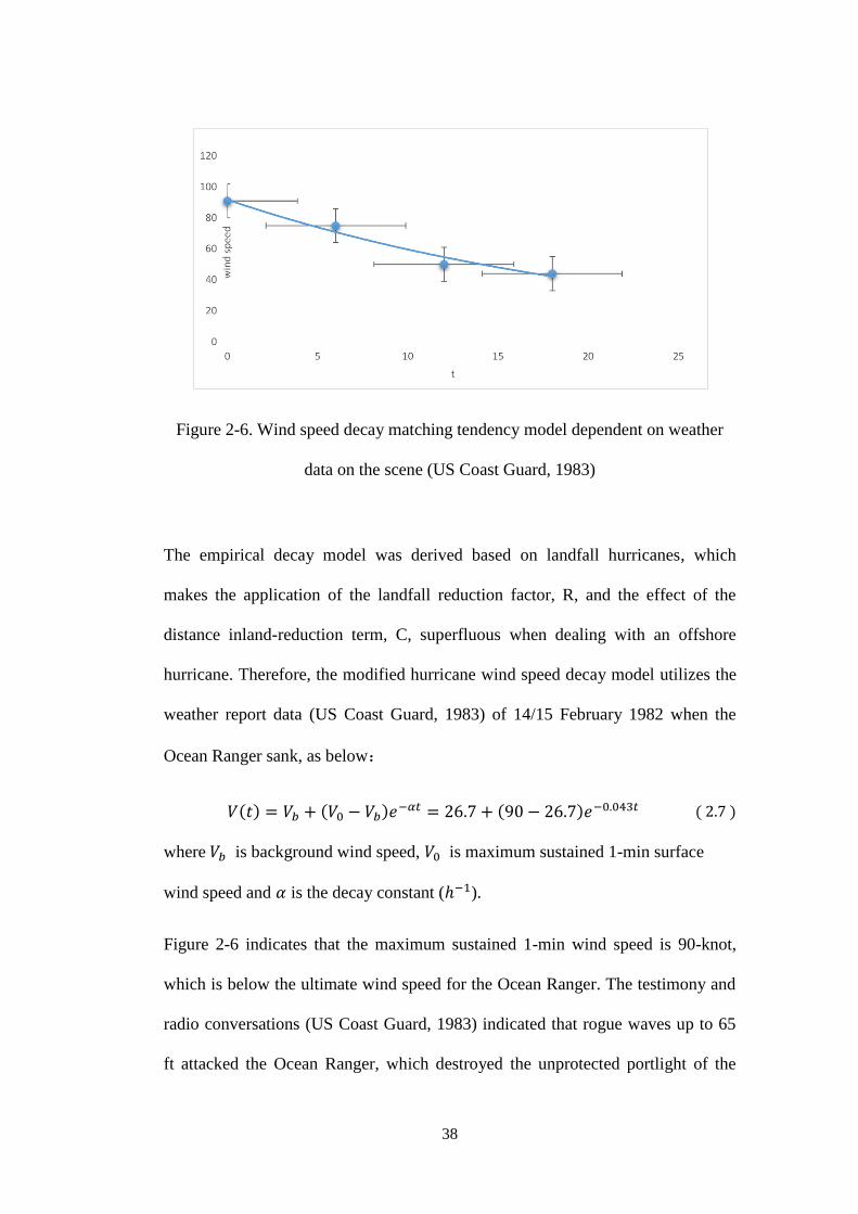
Figure 2-6. Wind speed decay matching tendency model dependent on weather

data on the scene (US Coast Guard, 1983)

The empirical decay model was derived based on landfall hurricanes, which

makes the application of the landfall reduction factor, R, and the effect of the

distance inland-reduction term, C, superfluous when dealing with an offshore

hurricane. Therefore, the modified hurricane wind speed decay model utilizes the

weather report data (US Coast Guard, 1983) of 14/15 February 1982 when the

Ocean Ranger sank, as below：

𝑉(𝑡) = 𝑉𝑏 + (𝑉0 − 𝑉𝑏)𝑒−𝛼𝑡 = 26.7 + (90 − 26.7)𝑒−0.043𝑡 ( 2.7 )

where 𝑉𝑏 is background wind speed, 𝑉0 is maximum sustained 1-min surface

wind speed and 𝛼 is the decay constant (ℎ−1).

Figure 2-6 indicates that the maximum sustained 1-min wind speed is 90-knot,

which is below the ultimate wind speed for the Ocean Ranger. The testimony and

radio conversations (US Coast Guard, 1983) indicated that rogue waves up to 65

ft attacked the Ocean Ranger, which destroyed the unprotected portlight of the

39

ballast control room.

Divide components’ sections and calculate corresponding 2.3.2

environmental loads

Figure 2-7. Schematic of the Ocean Ranger: derrick (a), middle and corner

column (b) and pontoon (c) with generated sections

As a semi-submersible offshore drilling unit, the Ocean Ranger consisted of

pontoons, derrick, supporting columns and main deck. Two pontoons, which

contained drill water, ballast water and fuel, provided floatation and rig power for

the unit. A total of eight columns consisting of four corner columns and four

middle columns supported the deck, and were located port and starboard,

40

respectively. The ballast control room was in the starboard middle column 28 ft

above the drilling draft, protected by deadlights. Two deck layers provided the

living space for crew and work areas, above which was the 185.4-ft high drilling

derrick. Figure 2-7 represents the generated structural units of the derrick, middle

and corner columns, and pontoons. Similar to the demonstration example, four

different sections are divided for derrick, corner column, and pontoons, while the

Ocean Ranger had four more middle columns and the ballast control room was

located at one of the middle columns. Noted that different components carry a

diverse combination of loads, except for the derrick. In this paper, it is clarified

that pontoons and columns under the operational draft suffer simultaneously from

the damage of wave load and sea pressure. Columns above the water line and deck

are buffeted by the combined impact of wave and wind loads. Ideally, the derrick

should only be exposed to wind attacks. Results of a variety of loads for design,

manufactured permissible condition and actual operating state are summarized in

Table 2-5.

Derive components’ probabilities of failure under combined loads 2.3.3

Probabilities of failure at components’ levels under single loads can be solved by

simultaneous equations of COV and substituting P and L in Equation (2.2) with an

annual probability of exceedance 10−2 and operational payload (loads of

affordable wind speed and wave height), respectively. It is assumed that the COV

of every section statistically distributed wind resistance response is 0.036 and the

COVs of statistically distributed wave resistance responses of corner column,

41

pontoon, deck and middle column are 0.15, 0.15, 0.30 and 0.20, respectively. The

sea pressure acting on the pontoon is higher than columns due to deeper water, the

COV of statistically distributed sea pressure resistance response of pontoon

(0.014) is smaller than columns (0.017) for the sake of manufacture safety

standards. Subsequently, Equation (2.3) uses the shape and location parameters of

Equation (2.2) with the assumed correlation coefficient ρ = 0 (wind and wave

independent assumption) to derive joint probabilities of failure for the joint

combined load. The probabilities of failure for every component section are

captured in Table 2-5.

As mentioned in the report (US Coast Guard, 1983), the deadlights, which should

have protected the porthole from wave impact, were open because of improper

operation. For this case, the strength reduction coefficient is introduced to model

the damage probability of the portlight. At first, the portlights and the deadlights

were regarded as a unit, designed and built to withstand 110-ft waves and 100-

knot winds simultaneously. Because of the improper operation, the portlight was

directly exposed to the harsh environments. Thus, the acceptable wave load of a

portlight should be reassessed. Based on DNVGL-OS-C201 (2017), the specific

minimum yield stress for normal strength steel is 235 MPa. However, the ultimate

permissible load on the protected portlight is 36.92 KPa because of configuration

and stress concentration. The maximum strength reduction coefficient is defined

as the ratio of the specific minimum yield stress to the permissible load.

𝑅𝑚 =𝜎𝑚

𝜎𝑃=

235𝑀𝑃𝑎

36.92 𝐾𝑃𝑎= 6368.56 ( 2.8 )

where 𝜎𝑚 is the specific minimum yield stress and 𝜎𝑃 is the permissible load.

42

The R𝑚 is 6,368.56 for deadlights. For the sake of reliability and accuracy, 50%

of the R𝑚 is applied to the portlight, which is made of tempered glass. ASTM

International (2018) stipulates the minimum surface compression for fully

tempered glass is 69 MPa. Therefore, the permissible load for a portlight is

2.17 × 104 Pa, as is shown in Table 2-5.

BN establishment and overall probabilities of failure estimation 2.3.4

Figure 2-8. BN of operational failure modeling of the Ocean Ranger

It is worth pointing out that middle columns are taken into consideration because

of the difference between the Ocean Ranger and the demonstration example. MS 1

– 4 represent the probabilities of failure of sections #1 to #4 of the middle column

43

caused by combined loads directly. MS2S represents both the direct damage and

collateral debris damage from adjacent section #1 of the middle column. Damage

to the derrick can destroy the deck due to objects falling from high altitudes.

Furthermore, without the support of middle and corner columns, the supporting

system cannot reinforce the deck. Columns are installed above the pontoons,

which explains that once the sections of columns connected to the pontoons fails,

related pontoon sections inevitably rupture. Then onboard liquid is influenced

because it is stored in the pontoon which further manages the buoyancy of the

SMU. Owing to a design flaw and improper operation, the ballast control room

where the portlights are installed is under the height of wave crests, which leads to

the failure of the deballast system. If the portlights are destroyed by a rogue wave,

seawater can inundate the ballast control room, causing the panel malfunction.

The panel which is protected by the portlight controls the pumping system and the

ballast valves system, which thereby control the onboard liquid.

Finally, damage probability modeling of the Ocean Ranger considering stability

and operational components is tailored in Figure 2-8 and Table 2-5 with CPTs

provided in the Appendix. The probabilities of failure (PoF) of several

aforementioned root nodes (Heising and Grenzebach, 1989), including valves,

pumps, ballast water, drilling water, and fuel, were utilized to analyze failure

probability using HUGIN 8.6 (http://www.hugin.com).

Results and Discussion 2.4

As can be seen from Table 2-5, wind load rises significantly along with the

increase of height, which is calculated as 3.51 kPa for section #1 of the derrick,

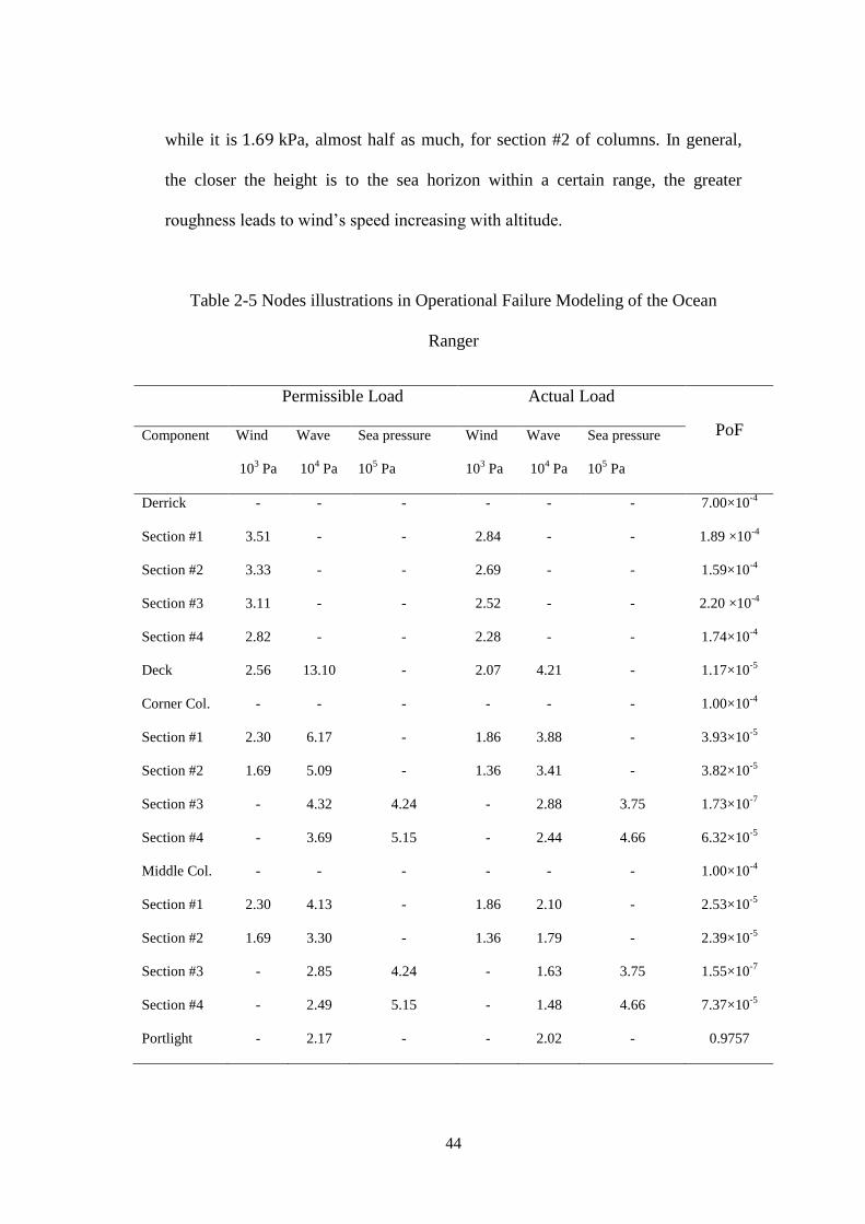
44

while it is 1.69 kPa, almost half as much, for section #2 of columns. In general,

the closer the height is to the sea horizon within a certain range, the greater

roughness leads to wind’s speed increasing with altitude.

Table 2-5 Nodes illustrations in Operational Failure Modeling of the Ocean

Ranger

Permissible Load Actual Load

PoF Component Wind

103 Pa

Wave

104 Pa

Sea pressure

105 Pa

Wind

103 Pa

Wave

104 Pa

Sea pressure

105 Pa

Derrick - - - - - - 7.00×10-4

Section #1 3.51 - - 2.84 - - 1.89 ×10-4

Section #2 3.33 - - 2.69 - - 1.59×10-4

Section #3 3.11 - - 2.52 - - 2.20 ×10-4

Section #4 2.82 - - 2.28 - - 1.74×10-4

Deck 2.56 13.10 - 2.07 4.21 - 1.17×10-5

Corner Col. - - - - - - 1.00×10-4

Section #1 2.30 6.17 - 1.86 3.88 - 3.93×10-5

Section #2 1.69 5.09 - 1.36 3.41 - 3.82×10-5

Section #3 - 4.32 4.24 - 2.88 3.75 1.73×10-7

Section #4 - 3.69 5.15 - 2.44 4.66 6.32×10-5

Middle Col. - - - - - - 1.00×10-4

Section #1 2.30 4.13 - 1.86 2.10 - 2.53×10-5

Section #2 1.69 3.30 - 1.36 1.79 - 2.39×10-5

Section #3 - 2.85 4.24 - 1.63 3.75 1.55×10-7

Section #4 - 2.49 5.15 - 1.48 4.66 7.37×10-5

Portlight - 2.17 - - 2.02 - 0.9757

45

Pontoons - - - - - - 2.00×10-4

Section #1 - 5.58 6.00 - 3.67 5.51 2.74×10-5

Section #2 - 5.58 6.00 - 3.67 5.51 2.74×10-5

Section #3 - 5.58 6.00 - 3.67 5.51 2.74×10-5

Section #4 - 5.58 6.00 - 3.67 5.51 2.74×10-5

Ocean Ranger - - - - - - 0.7812

Moreover, the average failure probability of sections for the derrick is 1.86 ×

10−4 . However, the average failure probabilities of sections for the deck,

columns, and pontoons are approximately 1.17 × 10−5 , 3.30 × 10−5 and

2.74 × 10−5 . In this regard, derrick section experienced a relatively high

probability of failure by almost one order of magnitude when compared to the

other structural components. In spite of the mutual interaction of adjacent sections

owing to the debris trajectory, the failure probability of the derrick, 7 × 10−4, is

still higher than for columns, 1 × 10−4, and pontoons, 2 × 10−4. The explanation

for this phenomenon can be found through the application of bivariate joint

probability distribution associated with the physical reliability model. Two

different indicators are combined, which is more accordant with the actual

situation than combining various types of loads directly. In other words, it is

dominated by the parameter which is closer to the maximum value and influenced

by the other one. In fact, deck, columns and pontoons suffer the impact from

either the wind-wave combined load or wave-sea pressure combined load. Ideally,

the derrick bears only the wind-induced load. In this case, the wind speed was 90

knots, which reached 90% of the maximum critical value and the wave height

was 65 ft, only accounting for 59% of the limit. Thus, wind speed in the

46

prevailing conditions was the dominant indicator resulting in the derrick having a

considerably high failure probability, while the wave height that was far beyond

the limit was the influenced parameter. Therefore, components that bore either the

load caused by the wave itself or the indirect dynamic sea pressure of each section

were less likely to fail.

Along with this line of consideration, the simulation results in Table 2-5 indicate

that the Ocean Ranger operated with an incredible probability of failure of 0.7812.

This is around 78 times as large as the lower limit of the operational failure

envelope. Logically speaking, if the estimated failure probability in the envelope

fell dramatically, termination of the operation to cease the risk should have been

adopted. On the contrary, probabilities of failure for the main structural

components such as the derrick, middle and corner columns, pontoons, etc. were

about 10−4. The calculated failure probability was still acceptable, which proved

that the Ocean Ranger could have survived the storm.

Nevertheless, due to inappropriate manual operations, the hurricane on 14/15

February 1982 destroyed the Ocean Ranger, unfortunately. As an improper

operating procedure, the deadlights, which should have protected the porthole

from wave impact, were open. As revealed by the reduction coefficient, the

permissible load of the portlight decreased significantly from 3.30 × 104 Pa to

2.17 × 104 Pa. What is even worse, the actual imposed load was 2.02 × 104 Pa,

which led ineluctably to the increase of probability of failure. The failure

probability of the exposed portlight was derived as 0.9757, which is nearly 41,000

times greater than is the case under protection. Subsequently, the branch which

follows the panel malfunction, failure of the pumping system and ballast valves,

47

severe listing, flooding of the chain locker and failure of the support system

occurred naturally. Because of the unexpected flooding of the chain locker room,

the failure probability of the supporting system rose sharply from 2 × 10−4 to

0.7810.

It is highlighted that the damage to the portlight which lacked the protection of

deadlights initiated the chain of events, in agreement with the Marine Casualty

Report (US Coast Guard, 1983). This signifies that in the actual operational

process, not only do the design and manufacturing characteristics of the platform

need to be taken into consideration, but also that human operation practices can

add considerable additional risk to the platform. Aiming to lower the damage

caused by improper manual operation from the inherent design to emergency

actions is essential. If feasible, it is recommended to strengthen the training,

knowledge, and instruction for proper operational procedures to enhance

reliability and mitigate potential hazards.

Conclusions 2.5

The proposed operational failure model is able to capture real-time weather data

and their impact on safe operation, which helps to promote safe and reliable

offshore development. It is highlighted that this study assesses the operational risk

of the semi-submersible mobile unit (SMU) quantitatively under combined wind

and wave induced loads with a probabilistic Bayesian network (BN) framework,

which represents conditional dependencies of the weather’s effect. More

specifically, it presents a detailed operational failure model considering the

48

combined loading of extreme weather conditions and the operational

characteristics of the SMU. Consistent and reliable results are provided, as

evidenced by the case study. As an anticipated risk estimation model, it is proved

that the proposed model is a useful and reliable tool to develop and monitor an

operational failure envelope of the SMU in given environmental conditions. For

the sake of improvement, it is recommended that more environmental loads such

as currents and sea ice induced loads should be taken into consideration to

simulate the operational disturbance for further research.

This paper has demonstrated the application of wind load response modeling, the

Morison model and the ultimate limit states method to estimate the combined

loading of extreme weather conditions imposed on the SMU. A physical

reliability model and joint probability distribution function have been

incorporated, which provide a deeper insight to capture the risk response. Along

with reducing the estimated failure probability through the implementation of BN

with the operational failure envelope in given environmental conditions, further

operational recommendations are suggested in order to avoid catastrophic disaster.

49

References 2.6

Abaei, M.M., Abbassi, R., Garaniya, V., Chai, S., Khan, F., 2018. Reliability

assessment of marine floating structures using Bayesian network. Applied Ocean

Research 76, 51-60.

Abaei, M.M., Arzaghi, E., Abbassi, R., Garaniya, V., Chai, S., Khan, F., 2018. A

robust risk assessment methodology for safety analysis of marine structures under

storm conditions. Ocean Engineering 156, 167-178.

ASTM International, 2018. ASTM C1048-18 Standard Specification for Heat-

Strengthened and Fully Tempered Flat Glass. ASTM International.

https://doi.org/10.1520/C1048-18.

Banks, M., Abdussamie, N., 2017. The response of a semisubmersible model

under focused wave groups: Experimental investigation. Journal of Ocean

Engineering and Science 2 (3), 161-171.

Barua, S., Gao, X., Pasman, H., Mannan, M.S., 2016. Bayesian network based

dynamic operational risk assessment. Journal of Loss Prevention in the Process

Industries 41, 399-410.

Bea, R., Iversen, R., Xu, T., 2001. Wave-in-deck forces on offshore platforms.

Journal of offshore mechanics and arctic engineering 123 (1), 10-21.

Cheng, E., Yeung, C., 2002. Generalized extreme gust wind speeds distributions.

Journal of Wind Engineering and Industrial Aerodynamics 90 (12-15), 1657-1669.

DNVGL-OS-C101, Design of offshore steel structures, general - LRFD method.

July 2019. DNV GL

50

DNVGL-OS-C201, Structural design of offshore units - WSD method. July 2017.

DNV GL

DNVGL-RP-C103, Column-Stabilised Units. July 2015. DNV GL

DNVGL-RP-C205, Enviromental conditions and enviromental loads. August

2017. DNV GL

Forbes, C., Evans, M., Hastings, N., Peacock, B., 2011. Statistical distributions.

4th ed. John Wiley & Sons, New Jersey, USA.

Ghafari, H., Dardel, M., 2018. Parametric study of catenary mooring system on

the dynamic response of the semi-submersible platform. Ocean Engineering 153,

319-332.

Gomathinayagam, S., Vendhan, C., Shanmugasundaram, J., 2000. Dynamic

effects of wind loads on offshore deck structures—a critical evaluation of

provisions and practices. Journal of Wind Engineering and Industrial

Aerodynamics 84 (3), 345-367.

Heising, C.D., Grenzebach, W.S., 1989. The ocean ranger oil rig disaster: A risk

analysis. Risk analysis 9 (1), 55-62.

Holmes, J.D., 2015. Wind loading of structures. CRC press, 3rd ed, Florida, USA.

HUGIN Expert Software Version 8.6, 2017. http://www.hugin.com.

Ismail, Z., Kong, K.K., Othman, S.Z., Law, K.H., Khoo, S.Y., Ong, Z.C., Shirazi,

S.M., 2014. Evaluating accidents in the offshore drilling of petroleum: Regional

picture and reducing impact. Measurement 51, 18-33.

Kaplan, J., DeMaria, M., 1995. A simple empirical model for predicting the decay

of tropical cyclone winds after landfall. Journal of applied meteorology 34 (11),

2499-2512.

51

Khakzad, N., Khan, F., Amyotte, P., 2012. Dynamic risk analysis using bow-tie

approach. Reliability Engineering & System Safety 104, 36-44.

Lee, J.-c., Jeong, J.-h., Wilson, P., Lee, S.-s., Lee, T.-k., Lee, J.-H., Shin, S.-c.,

2018. A study on multi-objective optimal design of derrick structure: Case study.

International Journal of Naval Architecture and Ocean Engineering 10 (6), 661-

669.

Leimeister, M., Kolios, A., 2018. A review of reliability-based methods for risk

analysis and their application in the offshore wind industry. Renewable and

Sustainable Energy Reviews 91, 1065-1076.

Liu, H., Sun, L., Huang, A., Zhao, Y., Chen, G., 2018. Performance-Based

Analysis of Wind-Survivability for Large Offshore Jacket Platforms Subject to

Hurricane, Paper Presented at the ASME 2018 37th International Conference on

Ocean, Offshore and Arctic Engineering. American Society of Mechanical

Engineers, Madrid, Spain.

Ma, J., Zhou, D., Han, Z., 2017. Wind and waves induced dynamic effects of a

semi-submersible platform, Paper Presented at the 27th International Ocean and

Polar Engineering Conference. International Society of Offshore and Polar

Engineers, San Francisco, USA.

Ma, J., Zhou, D., Han, Z., Zhang, K., Bao, Y., Dong, L., 2019. Fluctuating wind

and wave simulations and its application in structural analysis of a semi-

submersible offshore platform. International Journal of Naval Architecture and

Ocean Engineering 11 (1), 624-637.

Ma, J., Zhou, D., Han, Z., Zhang, K., Nguyen, J., Lu, J., Bao, Y., 2017. Numerical

simulation of fluctuating wind effects on an offshore deck structure. Shock and

52

Vibration. p. 3210271.

Song, G., Khan, F., Wang, H., Leighton, S., Yuan, Z., Liu, H., 2016. Dynamic

occupational risk model for offshore operations in harsh environments. Reliability

Engineering & System Safety 150, 58-64.

US Coast Guard, 1983. Marine Casualty Report: Mobile Offshore Drilling Unit

(MODU) Ocean Ranger, o.n. 615641 Capsizing and Sinking in the Atlantic Ocean,

on 15 February 1982 with Multiple Loss of life (No. USCG 16732/0001). U.S.

Department of Transportation, Washington, D.C.

Weber, P., Medina-Oliva, G., Simon, C., Iung, B., 2012. Overview on Bayesian

networks applications for dependability, risk analysis and maintenance areas.

Engineering Applications of Artificial Intelligence 25 (4), 671-682.

Yeo, C., Bhandari, J., Abbassi, R., Garaniya, V., Chai, S., Shomali, B., 2016.

Dynamic risk analysis of offloading process in floating liquefied natural gas

(FLNG) platform using Bayesian Network. Journal of Loss Prevention in the

Process Industries 41, 259-269.

Yu, Y., Hardowar, A., Yu, J., Hao, S., Gao, X., 2018. Investigation of TLP's

hydrodynamic response with different tendon connection angles. Theoretical and

Applied Mechanics Letters 8 (4), 291-297.

Zhang, S. (2017, August 25). When a hurricane hits an offshore oil platform:

Harvey could seriously damage oil and gas operations in the Gulf of Mexico. The

Atlantic: Science Edition Retrieved from: https://www.theatlantic.com/science/

archive/2017/08/harvey-offshore-platform-oil-gas/537960/

53

Appendix 2.7

The subjective belief is adapted to assign CPTs to reduce uncertainty, which is

sufficient to estimate the anticipated operational probability of failure for the

purpose of a safety reference. In short, the greater the height of the section, the

greater the mutual influence factor is, since the uppermost section has a strongest

potential of both kinetic and gravitational. Furthermore, it is assumed that only

two adjacent sections interact with the debris trajectory. As a consequence, Table

2-6 - Table 2-22 show the CPTs of the developed BN ( 𝑥�̅� represents the

damage/occurrence of component 𝑥𝑖 and W represents working condition, F

represents failure).

Table 2-6 The CPT of section #2, #3 and #4 for the derrick

#2 DS1 DS1̅̅ ̅̅ ̅ #3 DS2S DS2S̅̅ ̅̅ ̅̅ ̅ #4 DS3S DS3S̅̅ ̅̅ ̅̅ ̅

DS2 DS2̅̅ ̅̅ ̅ DS2 DS2̅̅ ̅̅ ̅ DS3 DS3̅̅ ̅̅ ̅ DS3 DS3̅̅ ̅̅ ̅ DS4 DS4̅̅ ̅̅ ̅ DS4 DS4̅̅ ̅̅ ̅

DS2S 1 0 0.49 0 DS3S 1 0 0.57 0 DS4S 1 0 0.65 0

DS2S̅̅ ̅̅ ̅̅ ̅ 0 1 0.51 1 DS3S̅̅ ̅̅ ̅̅ ̅ 0 1 0.43 1 DS4S̅̅ ̅̅ ̅̅ ̅ 0 1 0.35 1

Table 2-7 The CPT for the derrick

DS1 DS1̅̅ ̅̅ ̅

DS2S DS2S̅̅ ̅̅ ̅̅ ̅ DS2S DS2S̅̅ ̅̅ ̅̅ ̅

DS3S DS3S̅̅ ̅̅ ̅̅ ̅ DS3S DS3S̅̅ ̅̅ ̅̅ ̅ DS3S DS3S̅̅ ̅̅ ̅̅ ̅ DS3S DS3S̅̅ ̅̅ ̅̅ ̅

DS4S w F w F w F w F w F w F w F w F

Derrick 1 0 0 0 0 0 0 0 0 0 0 0 0 0 0 0

Derrick̅̅ ̅̅ ̅̅ ̅̅ ̅̅ 0 1 1 1 1 1 1 1 1 1 1 1 1 1 1 1

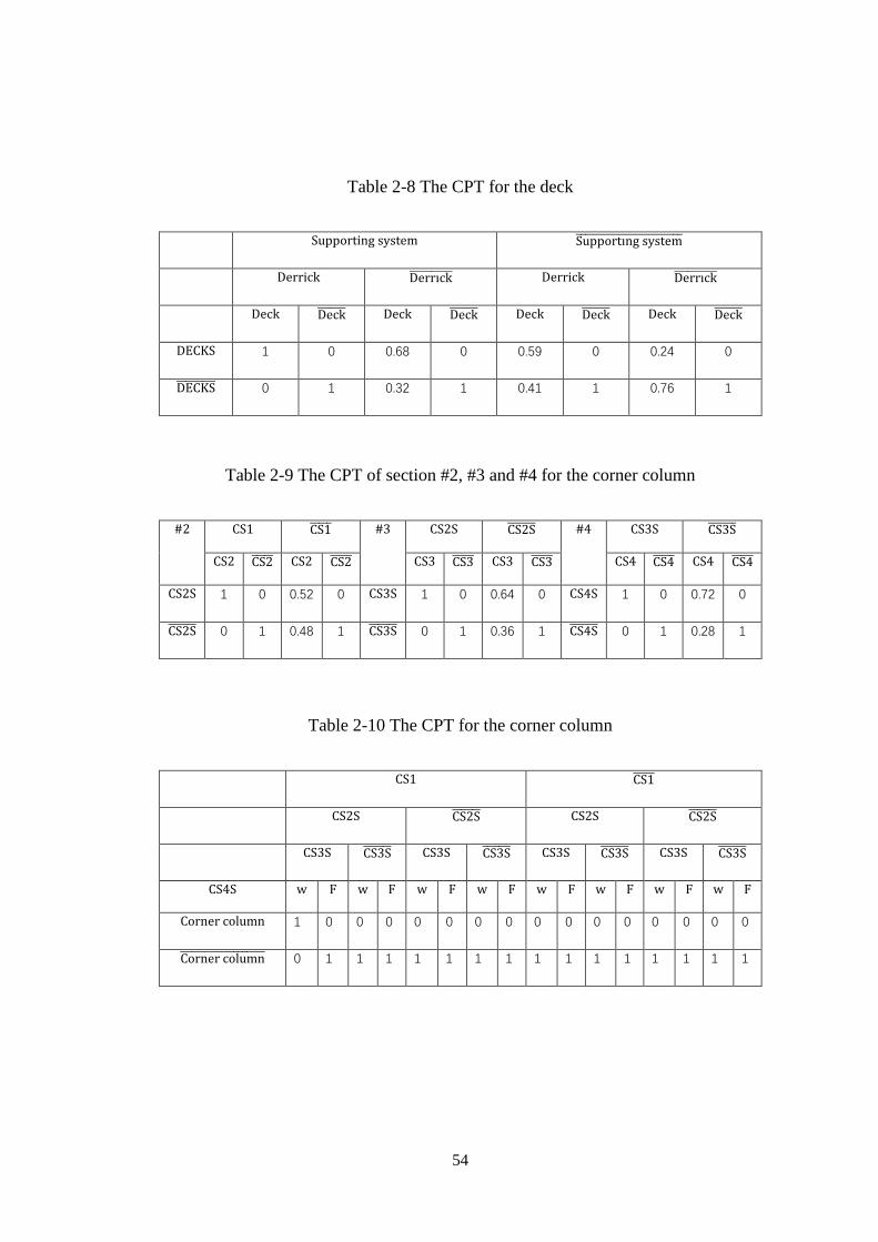
54

Table 2-8 The CPT for the deck

Supporting system Supporting system̅̅ ̅̅ ̅̅ ̅̅ ̅̅ ̅̅ ̅̅ ̅̅ ̅̅ ̅̅ ̅̅ ̅̅

Derrick Derrick̅̅ ̅̅ ̅̅ ̅̅ ̅̅ Derrick Derrick̅̅ ̅̅ ̅̅ ̅̅ ̅̅

Deck Deck̅̅ ̅̅ ̅̅ ̅ Deck Deck̅̅ ̅̅ ̅̅ ̅ Deck Deck̅̅ ̅̅ ̅̅ ̅ Deck Deck̅̅ ̅̅ ̅̅ ̅

DECKS 1 0 0.68 0 0.59 0 0.24 0

DECKS̅̅ ̅̅ ̅̅ ̅̅ ̅ 0 1 0.32 1 0.41 1 0.76 1

Table 2-9 The CPT of section #2, #3 and #4 for the corner column

#2 CS1 CS1̅̅ ̅̅ ̅ #3 CS2S CS2S̅̅ ̅̅ ̅̅ ̅ #4 CS3S CS3S̅̅ ̅̅ ̅̅ ̅

CS2 CS2̅̅ ̅̅ ̅ CS2 CS2̅̅ ̅̅ ̅ CS3 CS3̅̅ ̅̅ ̅ CS3 CS3̅̅ ̅̅ ̅ CS4 CS4̅̅ ̅̅ ̅ CS4 CS4̅̅ ̅̅ ̅

CS2S 1 0 0.52 0 CS3S 1 0 0.64 0 CS4S 1 0 0.72 0

CS2S̅̅ ̅̅ ̅̅ ̅ 0 1 0.48 1 CS3S̅̅ ̅̅ ̅̅ ̅ 0 1 0.36 1 CS4S̅̅ ̅̅ ̅̅ ̅ 0 1 0.28 1

Table 2-10 The CPT for the corner column

CS1 CS1̅̅ ̅̅ ̅

CS2S CS2S̅̅ ̅̅ ̅̅ ̅ CS2S CS2S̅̅ ̅̅ ̅̅ ̅

CS3S CS3S̅̅ ̅̅ ̅̅ ̅ CS3S CS3S̅̅ ̅̅ ̅̅ ̅ CS3S CS3S̅̅ ̅̅ ̅̅ ̅ CS3S CS3S̅̅ ̅̅ ̅̅ ̅

CS4S w F w F w F w F w F w F w F w F

Corner column 1 0 0 0 0 0 0 0 0 0 0 0 0 0 0 0

Corner column̅̅ ̅̅ ̅̅ ̅̅ ̅̅ ̅̅ ̅̅ ̅̅ ̅̅ ̅ 0 1 1 1 1 1 1 1 1 1 1 1 1 1 1 1

55

Table 2-11 The CPT for the supporting system

Chainlocker room Chainlocker room̅̅ ̅̅ ̅̅ ̅̅ ̅̅ ̅̅ ̅̅ ̅̅ ̅̅ ̅̅ ̅̅ ̅

Middle column Middle column̅̅ ̅̅ ̅̅ ̅̅ ̅̅ ̅̅ ̅̅ ̅̅ ̅̅ ̅ Middle column Middle column̅̅ ̅̅ ̅̅ ̅̅ ̅̅ ̅̅ ̅̅ ̅̅ ̅̅ ̅

Corner column w F w F w F w F

Supporting system 1 0 0 0 0 0 0 0

Supporting system̅̅ ̅̅ ̅̅ ̅̅ ̅̅ ̅̅ ̅̅ ̅̅ ̅̅ ̅̅ ̅̅ ̅̅ 0 1 1 1 1 1 1 1

Table 2-12 The CPT of section #2, #3 and #4 for the middle column

#2 MS1 MS1̅̅ ̅̅ ̅̅ #3 MS2S MS2S̅̅ ̅̅ ̅̅ ̅ #4 MS3S MS3S̅̅ ̅̅ ̅̅ ̅

MS2 MS2̅̅ ̅̅ ̅̅ MS2 MS2̅̅ ̅̅ ̅̅ MS3 MS3̅̅ ̅̅ ̅̅ MS3 MS3̅̅ ̅̅ ̅̅ MS4 MS4̅̅ ̅̅ ̅̅ MS4 MS4̅̅ ̅̅ ̅̅

MS2S 1 0 0.54 0 MS3S 1 0 0.66 0 MS4S 1 0 0.74 0

MS2S̅̅ ̅̅ ̅̅ ̅ 0 1 0.46 1 MS3S̅̅ ̅̅ ̅̅ ̅ 0 1 0.34 1 MS4S̅̅ ̅̅ ̅̅ ̅ 0 1 0.26 1

Table 2-13 The CPT for the middle column

MS1 MS1̅̅ ̅̅ ̅̅

MS2S MS2S̅̅ ̅̅ ̅̅ ̅ MS2S MS2S̅̅ ̅̅ ̅̅ ̅

MS3S MS3S̅̅ ̅̅ ̅̅ ̅ MS3S MS3S̅̅ ̅̅ ̅̅ ̅ MS3S MS3S̅̅ ̅̅ ̅̅ ̅ MS3S MS3S̅̅ ̅̅ ̅̅ ̅

MS4S w F w F w F w F w F w F w F w F

Middle column 1 0 0 0 0 0 0 0 0 0 0 0 0 0 0 0

Midle column̅̅ ̅̅ ̅̅ ̅̅ ̅̅ ̅̅ ̅̅ ̅̅ ̅̅ 0 1 1 1 1 1 1 1 1 1 1 1 1 1 1 1

56

Table 2-14 The CPT for the chainlocker room and the ballast valves system

Chainlocker room Corner column Corner column̅̅ ̅̅ ̅̅ ̅̅ ̅̅ ̅̅ ̅̅ ̅̅ ̅̅ ̅ Ballast valves system Ballast valves Ballast valves̅̅ ̅̅ ̅̅ ̅̅ ̅̅ ̅̅ ̅̅ ̅̅ ̅̅

List list̅̅ ̅̅ List list̅̅ ̅̅ Panel Panel̅̅ ̅̅ ̅̅ ̅ Panel Panel̅̅ ̅̅ ̅̅ ̅

Chainlocker room 1 0 0 0 Ballast valves system 1 0 0 0

Chainlocker room̅̅ ̅̅ ̅̅ ̅̅ ̅̅ ̅̅ ̅̅ ̅̅ ̅̅ ̅̅ ̅̅ ̅ 0 1 1 1 Ballast valves system̅̅ ̅̅ ̅̅ ̅̅ ̅̅ ̅̅ ̅̅ ̅̅ ̅̅ ̅̅ ̅̅ ̅̅ ̅̅ ̅ 0 1 1 1

Table 2-15 The CPT for the onboard liquid

Ballast valves system Ballast valves system̅̅ ̅̅ ̅̅ ̅̅ ̅̅ ̅̅ ̅̅ ̅̅ ̅̅ ̅̅ ̅̅ ̅̅ ̅̅ ̅

Ballast water capacity w F w F

Fuel tank capacity w F w F w F w F

Drilling water capacity w F w F w F w F w F w F w F w F

Onboard liquid 1 0 0 0 0 0 0 0 0 0 0 0 0 0 0 0

Onboard liquid̅̅ ̅̅ ̅̅ ̅̅ ̅̅ ̅̅ ̅̅ ̅̅ ̅̅ ̅̅ 0 1 1 1 1 1 1 1 1 1 1 1 1 1 1 1

Table 2-16 The CPT for the drilling water capacity and ballast water capacity

Pontoon Pontoon̅̅ ̅̅ ̅̅ ̅̅ ̅̅ ̅ Pontoon Pontoon̅̅ ̅̅ ̅̅ ̅̅ ̅̅ ̅

Ballast water Ballast water̅̅ ̅̅ ̅̅ ̅̅ ̅̅ ̅̅ ̅̅ ̅̅ ̅ Ballast water Ballast water̅̅ ̅̅ ̅̅ ̅̅ ̅̅ ̅̅ ̅̅ ̅̅ ̅ Drilling water Drilling water̅̅ ̅̅ ̅̅ ̅̅ ̅̅ ̅̅ ̅̅ ̅̅ ̅̅ Drilling water Drilling water̅̅ ̅̅ ̅̅ ̅̅ ̅̅ ̅̅ ̅̅ ̅̅ ̅̅

BWC 1 0 0 0 DWC 1 0 0 0

BWC̅̅ ̅̅ ̅̅ 0 1 1 1 DWC̅̅ ̅̅ ̅̅ ̅ 0 1 1 1

Table 2-17 The CPT for the fuel tank capacity and section #1 for the pontoon

Pontoon Pontoon̅̅ ̅̅ ̅̅ ̅̅ ̅̅ ̅ CC4S CC4S̅̅ ̅̅ ̅̅ ̅

Fuel Fuel̅̅ ̅̅ ̅̅ Fuel Fuel̅̅ ̅̅ ̅̅ PS1 PS1̅̅ ̅̅ ̅ PS1 PS1̅̅ ̅̅ ̅

57

Fuel tank capacity 1 0 0 0 PS1S 1 0 0.55 0

Fuel tank capacity̅̅ ̅̅ ̅̅ ̅̅ ̅̅ ̅̅ ̅̅ ̅̅ ̅̅ ̅̅ ̅̅ ̅ 0 1 1 1 PS1S̅̅ ̅̅ ̅̅ ̅ 0 1 0.45 1

Table 2-18 The CPT of section #2 for the pontoon

MC4S MC4S̅̅ ̅̅ ̅̅ ̅

PS1S PS1S̅̅ ̅̅ ̅̅ ̅ PS1S PS1S̅̅ ̅̅ ̅̅ ̅

PS2 PS2̅̅ ̅̅ ̅ PS2 PS2̅̅ ̅̅ ̅ PS2 PS2̅̅ ̅̅ ̅ PS2 PS2̅̅ ̅̅ ̅

PS2S 1 0 0.48 0 0.67 0 0.25 0

PS2S̅̅ ̅̅ ̅̅ ̅ 0 1 0.52 1 0.33 1 0.75 1

Table 2-19 The CPT of section #3 and #4 for the pontoon

#3 MC4S MC4S̅̅ ̅̅ ̅̅ ̅ #4 CC4S CC4S̅̅ ̅̅ ̅̅ ̅

PS2S PS2S̅̅ ̅̅ ̅̅ ̅ PS2S PS2S̅̅ ̅̅ ̅̅ ̅ PS3S PS3S̅̅ ̅̅ ̅̅ ̅ PS3S PS3S̅̅ ̅̅ ̅̅ ̅

PS3 PS3̅̅ ̅̅ ̅ PS3 PS3̅̅ ̅̅ ̅ PS3 PS3̅̅ ̅̅ ̅ PS3 PS3̅̅ ̅̅ ̅ PS4 PS4̅̅ ̅̅ ̅ PS4 PS4̅̅ ̅̅ ̅ PS4 PS4̅̅ ̅̅ ̅ PS4 PS4̅̅ ̅̅ ̅

PS3S 1 0 0.48 0 0.67 0 0.25 0 PS4S 1 0 0.48 0 0.55 0 0.08 0

PS3S̅̅ ̅̅ ̅̅ ̅ 0 1 0.52 1 0.33 1 0.75 1 PS4S̅̅ ̅̅ ̅̅ ̅ 0 1 0.52 1 0.45 1 0.92 1

Table 2-20 The CPT for the pontoon

PS1S PS1S̅̅ ̅̅ ̅̅ ̅

PS2S PS2S̅̅ ̅̅ ̅̅ ̅ PS2S PS2S̅̅ ̅̅ ̅̅ ̅

PS3S PS3S̅̅ ̅̅ ̅̅ ̅ PS3S PS3S̅̅ ̅̅ ̅̅ ̅ PS3S PS3S̅̅ ̅̅ ̅̅ ̅ PS3S PS3S̅̅ ̅̅ ̅̅ ̅

PS4S w F w F w F w F w F w F w F w F

Pontoon 1 0 0 0 0 0 0 0 0 0 0 0 0 0 0 0

Pontoon̅̅ ̅̅ ̅̅ ̅̅ ̅̅ ̅ 0 1 1 1 1 1 1 1 1 1 1 1 1 1 1 1

58

Table 2-21 The CPT for the pumping system

Panel Panel̅̅ ̅̅ ̅̅ ̅

Pump 1 Pump 1̅̅ ̅̅ ̅̅ ̅̅ ̅̅ Pump 1 Pump 1̅̅ ̅̅ ̅̅ ̅̅ ̅̅

Pump 2 Pump2̅̅ ̅̅ ̅̅ ̅̅ ̅ Pump 2 Pump2̅̅ ̅̅ ̅̅ ̅̅ ̅ Pump 2 Pump2̅̅ ̅̅ ̅̅ ̅̅ ̅ Pump 2 Pump2̅̅ ̅̅ ̅̅ ̅̅ ̅

Pumping system 1 1 1 0 0 0 0 0

Pumping system̅̅ ̅̅ ̅̅ ̅̅ ̅̅ ̅̅ ̅̅ ̅̅ ̅̅ ̅̅ ̅ 0 0 0 1 1 1 1 1

Table 2-22 The CPT for the Ocean Ranger

Pontoon Pontoon̅̅ ̅̅ ̅̅ ̅̅ ̅̅ ̅

Supporting system w F w F

Derrick w F w F w F w F

Deck system w F w F w F w F w F w F w F w F

Ocean ranger 1 0 0 0 0 0 0 0 0 0 0 0 0 0 0 0

Ocear ranger̅̅ ̅̅ ̅̅ ̅̅ ̅̅ ̅̅ ̅̅ ̅̅ ̅ 0 1 1 1 1 1 1 1 1 1 1 1 1 1 1 1

59

Chapter 3. Monitoring and Modeling of Environmental Load

Considering Dependence and Its Impact on the Failure

Probability2

Jinjie Fu and Faisal Khan*

Centre for Risk, Integrity and Safety Engineering (C-RISE),

Faculty of Engineering and Applied Science,

Memorial University of Newfoundland, St. John’s, NL, A1B 3X5, Canada

Abstract

Extreme weather conditions put heavy environmental loads on systems and may

cause catastrophic failure. Classification societies such as Lloyd’s Register, DNV

GL and the American Bureau of Shipping recommend methods for environmental

load calculations. These methods do not consider dependencies among parameters

when calculating environmental loads. This paper proposes a novel methodology

to consider the copula-based bivariate failure function to evaluate the dependence

structure of parameters and minimize uncertainty in load calculations. It also

presents a robust operational failure assessment model that considers real-time

environmental parameters along with their dependencies. The proposed

methodology and models are tested on a semi-submersible mobile unit (SMU).

2 Fu, J., & Khan, F. Monitoring and modeling of environmental load considering dependence and

its impact on the failure probability. Submitted to Ocean Engineering.

60

The failure probability corresponding to the wind and wave loads imposed on the

SMU is calculated using a physical reliability model and Bayesian network. The

copula-based bivariate failure function defines the dependence using the

parameters 𝛿 , which are estimated using maximum likelihood estimation. A

detailed case study illustrates the advantage of the proposed methodology. The

proposed method is of vital significance to developing a safe operating envelope

for offshore assets likely to face extreme weather conditions.

Keywords: Operational failure; Environmental loads; Dependence; Copula

function; Maximum likelihood estimation

61

Introduction 3.1

Hurricanes have become more frequent in the past few decades. In the 2005

Atlantic hurricane season, for example, the number of hurricanes recorded that

year, 15, broke the annual record set in 1969 [1]. The property damage and

economic losses that result from the landfall of hurricanes have also become more

severe. For example, Hurricane Katrina destroyed 44 offshore platforms [2] and

shut down many of the oil and gas production facilities located in the Gulf of

Mexico. Hence, research on environmental loads and their impact on the failure of

systems is of great importance to avoiding personal injury and property loss.

Classification societies suggest employing standards to calculate environmental

loads, such as those used by DNV GL [3] and the American Bureau of

Shipping (ABS) [4]. These standards provide effective and accurate results, are

widely applied, and have been proven to be effective in numerous engineering

practices. Suja-Thauvin et al. [5] used DNV GL standards to develop a

hydrodynamic load model that analyzes the mode response of a monopile offshore

wind turbine. Caille et al. [6] adopted and validated a hydrodynamics model based

on DNV GL methods for a tension leg platform (TLP) with inclined legs. Flis [7]

applied the provisions of the ABS and calculated the environmental loads for

cooling skid units. Li et al. [8] calculated wave loads in accordance with the ABS

rules of a 7th generation semi-submersible drilling unit (CSDU) to optimize its

structural configuration. However, the assessment of the dependencies among the

parameters to calculate environmental loads is lacking. In the case of actual

operation, these weather parameters have a certain interaction relationship,

62

particularly in harsh environments. This paper examines whether it underestimates

or overestimates the impact on the failure of the system.

In regard to dependence construction, the copula function is an emerging model.

Due to the complex interactions that occur in nature, the linear correlation

coefficient lacks the ability to ascertain the dependence among real-time

environmental parameters. The copulas overcome this limitation through the

capacity to model any dependence structures, and they have been widely used in

the field of financial investment, portfolio construction, and so on [9]. Recently,

scholars have applied the copula function to system safety and reliability

assessments [10-14]. Hashemi et al. [12] proposed a multivariate loss function

that combined the marginal loss functions with copulas for process facilities risk

analysis. Guo et al. [13] conducted a copula-based Bayesian network (CBBN)

model to analyze the process system that addressed the limitations of non-linear

dependence structures. Shen et al. [14] developed a mixed copula function to

acquire the dependence details among failure modes to analyze the reliability of a

gear door lock system. Here, the copula function is considered to propose an

innovative operational failure assessment model because of its flexibility.

This work calculates environmental loads using real-time weather data and

estimates the operational failure probability of the system. The dependence

structure between the real-time environmental parameters is described with copula

functions. The dependence parameters δ of the candidate copula models are

estimated using maximum likelihood estimation. Then, the Akaike’s information

criterion (AIC) differences and Akaike weight are used to select the best copula

63

model to depict the dependence structure between the parameters to calculate the

environmental loads. The comparison results of the case study demonstrate the

flexibility and significance of the proposed model.

The structure of this paper is described as follows. Section 3.2 explains the

procedure of the proposed real-time environmental load and its impact

considering the dependence model with a simple illustrative example. Then,

Section 3.3 applies the proposed model to a typical semi-submersible mobile unit

(SMU) as a case study to demonstrate its general applicability. The results of the

copula-based bivariate failure function and independent load failure function are

compared and discussed in Section 3.4. The main findings of the study are

summarized in Section 3.5.

The Proposed Methodology 3.2

The practical applicability of operational failure assessment with real-time

weather observation is highlighted using a copula-based dependence function. The

copula function defines the dependence between the parameters to calculate

environmental loads in this paper. Figure 3-1 shows the details of the proposed

methodology. The steps of the proposed methodology are explained with a simple

example.

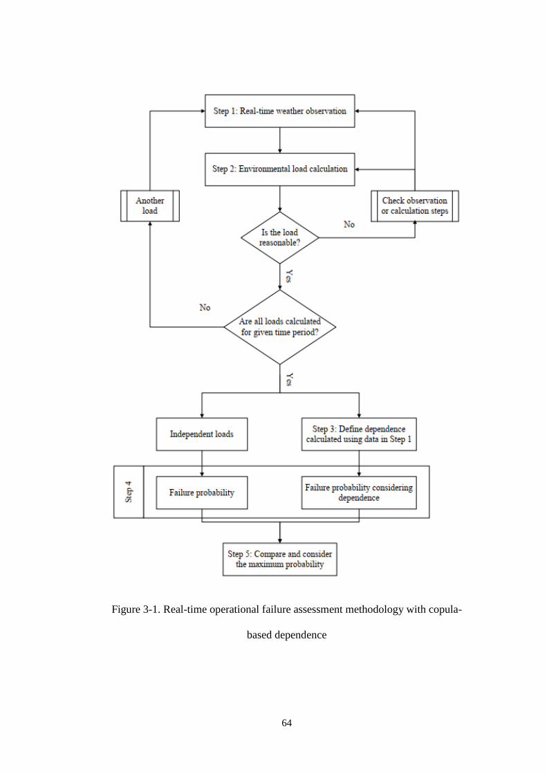
64

Figure 3-1. Real-time operational failure assessment methodology with copula-

based dependence

65

3.2.1 Step 1: Real-time weather observation

As the basis of the proposed model, the first step is to gain access to real-time

weather data. The environmental loads calculated in this paper are wind loads and

wave loads. Therefore, 500 sets of wave data and concurrent meteorological

observation data were obtained from wave data available online from the

Department of Fisheries and Oceans Canada (DFO) [15]. Figure 3-2 plots an

example with wind speed and wave height.

Figure 3-2. Scatter plot of the wind speed and wave height example

3.2.2 Step 2: Environmental load calculation

Once the real-time weather data are obtained, the environmental loads are

calculated with the corresponding model. It is suggested from DNVGL-RP-C205

[3] that the wind and wave-induced loads are estimated from the wind load

modeling and Morison wave load model, respectively.

0

2

4

6

8

10

12

14

16

0 5 10 15 20 25

Wav

e H

eigh

t (m

)

Wind Speed (m/s)

66

Figure 3-3. Schematic of the sample object with different sections

Table 3-1 shows the physical characteristics of the sample object. As revealed in

Figure 3-3, the sample object is used to demonstrate the proposed methodology.

The sample object consists of a pontoon and a column. The pontoon provides

flotation to the system and supports other functional structure components, which

are simplified as a column on the top of it. To further evaluate the impact of the

environmental loads on the failure of the system, each structural component is

divided into several sections that form the root causes of the Bayesian network

(BN).

Table 3-1 Physical characteristics of the sample object

Component Parameter Value Component Parameter Value

Column

Height 24 m

Pontoon

Height 8 m

Diameter 10 m Length 45 m

67

Waterline Depth 16 m Width 15 m

Winds Maximum 30 m/s Waves Maximum 30 m

The sections for the column are trisected according to the height, as presented in

Figure 3-3. Similarly, generated sections #1, #2 and #3 of the pontoon are divided

by the length.

3.2.3 Step 3: Define dependence calculated using data in Step 1

Along this line of consideration, the procedure followed is the dependence

assessment. The copula was first proposed by Sklar [16] in 1959 and is known as

the theorem of Sklar. It has been shown that copula is a robust tool for assessing

the dependence among random variables by establishing the joint distribution.

Because it is a marginal distribution-free model, it is capable of capturing the

dependence directly from the sample data. In other words, copula-based

dependence assessment allows the combination of a variety of types of d-

dimensional marginal distributions.

Here, the bivariate case is used to analyze the dependence structure between wind

speed and wave height, which are the dominant parameters used to calculate the

wind loads and wave loads, respectively.

𝐹(𝑥1, 𝑥2) = 𝐶(𝐹1(𝑥1), 𝐹2(𝑥2)) (3.1)

The joint distribution function is expressed in Equation (3.1). Two random

variables are represented as x1and x2. Then, the copula function C is written in

Equation (3.2).

68

𝐶(𝜇1, 𝜇2) = 𝐹(𝐹1−1(𝜇1), 𝐹2

−1(𝜇2)) = ∫ ∫ 𝑐(𝑥, 𝑦)𝑑𝑥𝑑𝑦𝜇2

−∞

𝜇1

−∞ (3.2)

Where, c(x, y) is the density of the copula.

Compared with implicit copulas such as Gaussian copula, Archimedean copula

family [17] are defined as explicit copulas with simple closed forms. This makes

them suitable for low-dimensional joint distribution. Three examples of

Archimedean copulas [18] are the Clayton copula, the Frank copula and the

Gumbel copula.

𝐶𝐶𝑙𝑎𝑦𝑡𝑜𝑛(𝜇1, 𝜇2) = (𝜇1−𝛿 + 𝜇2

−𝛿 − 1)−

1

𝛿 (3.3)

Where, δ ∈ [−1, ∞) \ {0}.

𝐶𝐹𝑟𝑎𝑛𝑘(𝜇1, 𝜇2) = −1

𝛿𝑙𝑛 (1 +

(𝑒−𝛿𝜇1−1)(𝑒−𝛿𝜇2−1)

𝑒−𝛿−1) (3.4)

Where, δ ∈ (−∞, ∞) \ {0}.

𝐶𝐺𝑢𝑚𝑏𝑒𝑙(𝜇1, 𝜇2) = 𝑒𝑥𝑝 {−((− 𝑙𝑛(𝜇1))𝛿 + (− 𝑙𝑛(𝜇2))𝛿)1

𝛿} (3.5)

Where, δ ∈ [1, ∞).

δ explains the dependence information between the random variables μ1 and μ2.

The Clayton copula, the Frank copula, and the Gumbel copula have lower tail

dependence, radial symmetry, and upper tail dependence, respectively. Therefore,

nearly all the tail dependences can be estimated by the three copula candidate

models.

Logically, the next thing to do is to determine the parameters δ efficiently and

precisely. The canonical maximum likelihood method (CML) [19] is introduced

here. The main advantage of the copula function is that the error caused by the

69

improper choice of the marginal distributions can be avoided. The semiparametric

method CML satisfies the goal of estimating the parameters δ directly from the

data sets.

The copula density is used to calculate the pseudo log-likelihood function.

Symbolic expressions of the bivariate copula density for the three candidate

models are addressed with the help of MATLAB [20]. For example, the copula

density for the Clayton copula is shown in Equation (3.6).

𝑐(𝜇1, 𝜇2) =𝜕2𝐶𝐶𝑙𝑎𝑦𝑡𝑜𝑛(𝜇1,𝜇2)

𝜕𝜇1𝜕𝜇2= (1 + 𝛿)(𝜇1𝜇2)−𝛿−1(𝜇1

−𝛿 + 𝜇2−𝛿 − 1)

−1

𝛿−2

(3.6)

Following this, μ1 and μ2 are the uniform marginal variates. It can be solved by

the rescaled empirical distribution function by means of the indicator function, as

is shown in Equation (3.7).

𝜇 = 𝐹(𝑥) =∑ 1(𝑋𝑖≤𝑥)𝑛

𝑖=1

𝑛+1 (3.7)

Where n is the sample data size.

Ultimately, the parameter δ is confirmed by forming and maximizing the pseudo

log-likelihood function (LLF), which is written in Equation (3.8).

𝛿 = 𝑎𝑟𝑔 𝑚𝑎𝑥 𝐿𝐿𝐹(𝛿) = ∑ 𝑙𝑛 (𝑐(𝜇1, 𝜇2))𝑛𝑖=1 (3.8)

For the sake of method demonstration, the dependence function between the wind

speed and wave height in Figure 3-2 is used as an example application. Figure 3-4

presents the transformed data sample results using the rescaled empirical

distribution function.

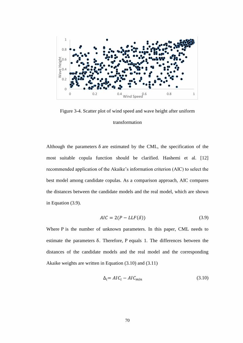
70

Figure 3-4. Scatter plot of wind speed and wave height after uniform

transformation

Although the parameters δ are estimated by the CML, the specification of the

most suitable copula function should be clarified. Hashemi et al. [12]

recommended application of the Akaike’s information criterion (AIC) to select the

best model among candidate copulas. As a comparison approach, AIC compares

the distances between the candidate models and the real model, which are shown

in Equation (3.9).

𝐴𝐼𝐶 = 2(𝑃 − 𝐿𝐿𝐹(𝛿)) (3.9)

Where P is the number of unknown parameters. In this paper, CML needs to

estimate the parameters δ. Therefore, P equals 1. The differences between the

distances of the candidate models and the real model and the corresponding

Akaike weights are written in Equation (3.10) and (3.11)

∆𝑖= 𝐴𝐼𝐶𝑖 − 𝐴𝐼𝐶𝑚𝑖𝑛 (3.10)

0

0.2

0.4

0.6

0.8

1

0 0.2 0.4 0.6 0.8 1

Wav

e H

eigh

t

Wind Speed

71

It is natural that the candidate model with the smallest ∆i is the most suitable

model. In other words, the greater the ∆i, the further the distance between the

candidate model and the best model.

𝑤𝑖 =𝑒𝑥𝑝 (−0.5∆𝑖)

∑ 𝑒𝑥𝑝 (−0.5∆𝑟)𝑅𝑟=1

(3.11)

Another alternative selection method [21] is the Akaike weight wi, where R is the

number of candidate copulas. Thus, the weight wi is influenced by the candidate

number. The larger the wi, the more evident it is that the corresponding model is

the exact model.

Table 3-2 CML and model selection calculation results

Copula 𝜹 𝑳𝑳𝑭(𝜹) 𝐀𝐈𝐂 ∆𝒊 𝒘𝒊

Clayton 0.568 35.177 -68.354 144.878 0

Frank 3.786 80.878 -159.756 53.476 0

Gumbel 1.617 107.616 -213.232 0 1

Table 3-2 shows the example results calculated from the maximum log-likelihood

function and best model selection methods: AIC differences and Akaike weights.

As can be seen, the AIC differences and the Akaike weights show substantial

evidence that the Gumbel copula model is sufficient to describe the dependence

structure between the 500-set example for wind speed and wave height.

Accordingly, the CML and AIC with associated AIC differences and Akaike

weights are able to capture the dependence function among bivariate distributed

72

random variables. Therefore, it is suitable for assessing the dependence structure

between the parameters to calculate the loads induced by wind and waves.

3.2.4 Step 4: Failure probability calculation

From Steps 1 to 3, the environmental loads and dependence structure between

parameters used to calculate the environmental loads are clarified. Therefore, how

to evaluate the imposed environmental loads of each section quantitatively with

probabilities is of great significance.

Ebeling [22] put forward the physical reliability model, which can assess the

failure probability of structures, mechanical facilities and so on. It is assumed that

either stress or strengthen or both of them follow specific types of distributions.

Each divided section is made up of many nodes, each of which has different

resistances to wind-induced loads and wave-induced loads. The resistances should

be no less than zero. Thus, it is assumed that both resistances to wind-induced

loads and wave-induced loads of a particular section follow the lognormal

distributions.

𝑃(𝑓𝑎𝑖𝑙𝑢𝑟𝑒) = ∫ 𝑓𝑟(𝑟)𝐿

0𝑑𝑟 = 𝛷(

1

𝑠𝑙𝑛

𝐿

𝑡𝑚𝑒𝑑) (3. 12)

Equation (3.12) explains that the failure probability is calculated through the

integration of the resistance from zero to the load. When the wind speed is

30 m/s or the wave height is 30 m (maximum design and manufactured

environmental parameters for the sample object), the wind or wave loads

correspond to the failure probabilities 10−2, as recommended by DNVGL-OS-

C101 [23]. The coefficient of variation (CV) is also used to derive the unknown

73

parameters of the lognormal distribution.

Figure 3-5. Node's resistance response to environmental loads with different CVs

Figure 3-5 shows the influence of the CV. Intuitively, the higher the CV, the more

sensitive to the loads the section is. Robert Bea (a professor emeritus at the

University of California, Berkeley) observed [24] that “cresting waves will do real

damage” when compared to wind and rainfall. Thus, the CV of wave load

resistance is greater than the CV of wind load resistance for the section under the

impact of combined loads. In this example case, it is assumed that the CV of wave

load resistance is 0.132 and the CV of wind load resistance is 0.108 for section #2

of the column. When compared to the pontoon and section #3 of the column, the

wave forces imposed on section #3 are smaller. From the perspective of operation,

the sample object has the ability to withstand the designed maximum wave height

as a whole system, which means the column and pontoon are all in normal

operating conditions. Therefore, the failure probabilities should be at a similar

magnitude. It is assumed that the CV of wave load resistances for the pontoon and

74

section #3 of the column are 0.083 and 0.068, respectively, and the CV of wind

load resistance for section #1 of the column is 0.101 for the sake of manufacture

safety standards.

Table 3-3 Environmental loads for the sample object

Structure Level

Maximum Bearable

Loads

Example loads

Component

Section

Number

Wind

102 Pa

Wave

104 Pa

Wind

102 Pa

Wave

104Pa

Column

#1 7.75 5.36 4.06 -

#2 5.69 4.53 2.98 3.01

#3 - 3.83 - 2.48

Pontoon

#1 - 5.17 - 3.05

#2 - 5.17 - 3.05

#3 - 5.17 - 3.05

Sample data (wind speed 21.7 m/s, wave height 14.3 m) from Figure 3-2 are

used as example environmental parameters to calculate the environmental loads

and failure probabilities. The results are shown in Table 3-3 and Table 3-4.

3.2.5 Step 5: Compare and consider the maximum probability of failure

The failure probabilities for every section are calculated through the physical

reliability model, and the next step is to derive the failure probabilities from the

75

level of sections to the level of components and from the level of components to

the system. Bayesian network (BN) is a causal inference model capable of

integrating the overall probability with the help of nodes, arcs and conditional

probability tables (CPTs) [25]. It is demonstrated in Figure 3-6 that root causes

represent the failure probabilities from the level of sections. The arcs represent the

causal relationships among nodes that are achieved mathematically by the CPTs.

Figure 3-6. BN for the sample object

As mentioned before, the main structural components of the sample object include

a column and pontoon. As shown in Figure 3-3, the pontoon and column have

three sections, which are represented as PS1 – 3 and CS1 - 3. The suffix “S” refers

to damage caused by debris from adjacent sections.

Table 3-4 Failure probabilities using the example sample data

Node Probability Node Probability

76

Column

Independent 7.12 × 10−5 Pontoon 9.25 × 10−5

Column

Copula Dependent 6.00 × 10−4 Section #1 2.68 × 10−5

Section #1 2.18 × 10−5 Section #2 2.68 × 10−5

Section #2

Independent 2.58 × 10−5 Section #3 2.68 × 10−5

Section #2

Copula Dependent 5.96 × 10−4

Sample Object

Independent 2.00 × 10−4

Section #3 2.36 × 10−5

Sample Object Copula

Dependent 8.00 × 10−4

Clearly, both wind load and wave load act on the sections #2 (column) of the

sample object. The failure probability considering dependent loads (the

dependence between the parameters to calculate the environmental loads is

defined in Step 3) should be addressed by the copula-based bivariate failure

function in Equation (3.13). On the contrary, the failure probability assuming

independent loads is calculated by the bivariate lognormal distribution with

correlation coefficient 𝜌 equals to 0.

𝐵𝐹𝐹(𝑃1, 𝑃2) = 𝑓1(𝑃1) × 𝑓2(𝑃2) × 𝑐(𝐹1(𝑃1), 𝐹2(𝑃2)) (3.13)

Where BFF(P1, P2) is the bivariate failure density function, P1 and P2 are

parameters to calculate wind loads and wave loads, 𝑓(𝑃) is the load calculation

model and physical reliability model, and c(F1(𝑃1), 𝐹2(𝑃2)) is the copula-based

dependence function.

77

Figure 3-7. Failure probability of section #2 (column) with dependent and

independent loads

The failure probabilities of the components and the sample object are presented in

Table 3-4. The failure probabilities of section #2 of the column are shown in

Figure 3-7. The failure probability considering dependent loads is greater than the

failure probability with independent loads assumption. It is calculated in Step 3

that the dependence between the wind speed and wave height for the example data

sample is established by the Gumbel copula. The results reveal that the failure

probability estimated considering independent environmental loads is an

underestimation. It is therefore crucial to take dependence into consideration to

provide a safety operational envelope using the copula-based bivariate failure

function.

2.5

8E-

05

5.9

6E-

04

SECTION #2

Independent

Copula dependent

78

Application of the proposed methodology 3.3

The proposed methodology is applied to a typical semi-submersible mobile unit

(SMU) operating in the Grand Banks to identify a safety operating envelope. The

results are compared with the traditional approach.

3.3.1 Steps 1-2: Real-time weather observation and environmental load

calculation

In this paper, 1000 sets of wave data and concurrent meteorological observation

data from the buoy: Banquereau – 44139 are used from the wave data available

on-line from the Department of Fisheries and Oceans Canada (DFO) [15]. Figure

3-8 presents the wind speed and wave height observed from Banquereau – 44139.

Figure 3-8. Scatter plot of wind speed and wave height for Banquereau – 44139

As the basis of the proposed modelling, it is necessary to clarify the geometric

0

2

4

6

8

10

12

14

16

0 5 10 15 20 25

Wav

e H

eigh

t (m

)

Wind Speed (m/s)

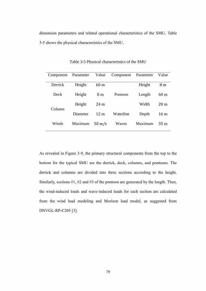
79

dimension parameters and related operational characteristics of the SMU. Table

3-5 shows the physical characteristics of the SMU.

Table 3-5 Physical characteristics of the SMU

Component Parameter Value Component Parameter Value

Derrick Height 60 m

Pontoon

Height 8 m

Deck Height 8 m Length 60 m

Column

Height 24 m Width 20 m

Diameter 12 m Waterline Depth 16 m

Winds Maximum 50 m/s Waves Maximum 35 m

As revealed in Figure 3-9, the primary structural components from the top to the

bottom for the typical SMU are the derrick, deck, columns, and pontoons. The

derrick and columns are divided into three sections according to the height.

Similarly, sections #1, #2 and #3 of the pontoon are generated by the length. Then,

the wind-induced loads and wave-induced loads for each section are calculated

from the wind load modeling and Morison load model, as suggested from

DNVGL-RP-C205 [3].

80

Figure 3-9. Schematic of the typical SMU with generated sections

3.3.2 Step 3: Define dependence calculated using data in Step 1

The crux of the proposed methodology is to deduce the dependence function

between the parameters to calculate the environmental loads. In practical

situations, the occurrence of the surge is usually related to extreme wind. Hence, it

is of considerable significance to consider the dependence to construct the

bivariate failure function.

81

Figure 3-10. Scatter plot of wind speed and wave height after uniform

transformation for Banquereau – 44139

Following the rescaled empirical distribution function in Equation (3.7), the

uniform transformed marginals of wind speed and wave height are shown in

Figure 3-10. To describe the dependence structure to the greatest extent possible,

three copula models from the Archimedean family are filtered out as potential

candidates for their ability to reflect lower tail dependence, radial symmetry, and

upper tail dependence.

Table 3-6 CML and model selection calculation results for 1000 sets of data from

the buoy: Banquereau – 44139

Copula 𝜹 𝑳𝑳𝑭(𝜹) 𝐀𝐈𝐂 ∆𝒊 𝒘𝒊

Clayton 0.498 57.591 -113.182 284.378 0

Frank 3.475 138.265 -274.530 123.030 0

Gumbel 1.573 199.780 -397.560 0.000 1

0

0.2

0.4

0.6

0.8

1

0 0.2 0.4 0.6 0.8 1

Wav

e H

eigh

t

Wind Speed

82

Then, the uniform marginals are substituted into the copula density, which is

processed using MATLAB. The dependence parameters δ are calculated using

maximum likelihood estimation with Equation (3.8). Afterward, the AIC value,

AIC difference ∆i and Akaike weights wi are presented in Table 3-6.

In view of the best model selection criteria, convincing evidence is shown that the

Gumbel copula is the closest model to the true model. Generally speaking, the

larger AIC difference ∆𝑖 is, the smaller the Akaike weight 𝑤𝑖 is, and the farther

the distance between the candidate model and the true model. Based on the rules

of thumb proposed by Burnham and Anderson [21], the level of support for the

candidate model is essentially none if ∆𝑖is larger than 10. The Gumbel copula is

selected to describe the dependence structure between the parameters to calculate

the environmental loads. It is also apparent from Figure 3-8 and Figure 3-10 that

the occurrence of strong winds is always accompanied with rogue waves. In

summary, the upper tail dependence between the wind speed and wave height is

captured by the Gumbel copula.

3.3.3 Step 4-5: Failure probability calculation and comparison

As mentioned before, the main structural components of the SMU include the

derrick, deck, columns and pontoons. The derrick raises and lowers drilling tools,

while the deck stores the generator room, machine equipment and so on. Due to

the support of columns that connect the deck and pontoons (the sources of the

83

floatation), the SMU is a column-stabilized mobile unit.

Figure 3-11. Tailored BN for the SMU

Consequently, the construction of the BN follows the unit configuration logic as

shown in Figure 3-11 . In general, the tailored BN consists of four parts, which

illustrate the four subsystems: the pontoon, column, derrick, and deck. As shown

in Figure 3-9 , the pontoon, column and derrick have three sections, which are

represented as PS1 – 3, CS1 – 3, and DS1 – 3 in the BN. Apart from the necessary

sections, the mutual dependences are considered as distinguished with the suffix

“S”. Due to the fact that falling debris may destroy the adjacent sections, the

lower sections suffer damage from environmental loads directly and debris from

adjacent higher sections. The damage dependences are adopted from the CPTs in

Fu’s research [26]. Without the stabilization of the columns, the deck could not

bear the derrick. In addition, falling debris from the derrick may hit the deck,

which would further threaten the integrity of the deck. The subsystem of the

84

pontoon is responsible for floatation. Accordingly, failure of any one of the

abovementioned components would result in the failure of the SMU.

To display the advantage of the operational failure assessment for the SMU

considering dependent environmental loads, a comparison study is conducted

using one sample of data (wind speed 25 m/s, wave height 16.1 m) as a case

example. The maximum bearable environmental loads for the SMU are calculated

with the design and manufactured maximum allowable parameters: wind speed

50 m/s, wave height 35 m. It is recommended by DNVGL-OS-C101 [23] that the

corresponding failure probabilities be 10−2. For the sake of simplicity, the CVs

for the sections impacted by combined environmental loads are assumed as 0.295

for the wave load resistances and 0.222 for the wind load resistances. Table 3-7

shows the results of the maximum bearable environmental loads and the case

example loads for the SMU.

As can be seen, sections #1 and #2 of the column are impacted by wind loads and

wave loads simultaneously using the example case data. The copula-based

bivariate failure function as expressed in Equation (3.13) is used to calculate the

failure probability considering dependent loads. For the purpose of comparison,

the failure probability assuming the independent loads is solved by the joint

bivariate lognormal distribution (𝜌 = 0). In brief, the probabilities of the nodes in

the Bayesian network are summarized in Table 3-8 . The comparison results are

shown in Figure 3-12.

Results and Discussion 3.4

Table 3-7 shows that the actual environmental loads are less than the maximum

85

bearable loads because of the small wind speed and low wave height. Following

this, the failure probabilities in Table 3-8 reveal that the SMU operates within the

bounds of safety permission under the circumstances of wind speed 25 m/s and

wave height 16.1 m, as the corresponding failure probability is merely 3.00 ×

10−4. The failure probability for the component derrick is 7.75 × 10−5 under the

impact of wind load only. The failure probabilities of the column and pontoon are

7.74 × 10−5 and 8.02 × 10−5 , respectively, which are nearly at the same

magnitude.

Table 3-7 Environmental loads for the SMU

Structure Level

Maximum Bearable

Loads

Case Example

loads

Component

Section

Number

Wind

103 Pa

Wave

104 Pa

Wind

102 Pa

Wave

104Pa

Derrick

#1 3.34 - 8.36 -

#2 3.10 - 7.74 -

#3 2.77 - 6.92 -

Deck - 2.44 13.8 6.10 -

Column

#1 2.15 7.02 5.38 4.53

#2 1.58 5.99 3.95 4.07

#3 - 5.11 - 3.35

Pontoon

#1 - 7.74 - 4.58

#2 - 7.74 - 4.58

86

#3 - 7.74 - 4.58

However, Figure 3-12 demonstrates the superiority of assessing the load impact

on the failure of the system considering the dependence among parameters to

calculate environmental loads. As is shown in Figure 3-12, the failure

probabilities of sections #1 and #2 calculated by the copula-based bivariate failure

function are approximately fifty times larger than the one with the independent

loads assumption. The failure probability of the SMU is integrated with the aid of

the BN. Consequently, the failure probability of the SMU considering dependent

loads is 10 times greater than the one without taking dependence into account (𝜌 =

0).

Table 3-8 Nodes probabilities of the Bayesian network

Node Probability Node Probability

Derrick 7.75 × 10−5

Section #2

Independent 2.77 × 10−5

Section #1 2.66 × 10−5

Section #2

Copula Dependent 1.42 × 10−3

Section #2 2.53 × 10−5 Section #3 2.31 × 10−5

Section #3 2.56 × 10−5 Pontoon 8.02 × 10−5

Deck 2.60 × 10−5 Section #1 2.26 × 10−5

Column

Independent 7.74 × 10−5 Section #2 2.26 × 10−5

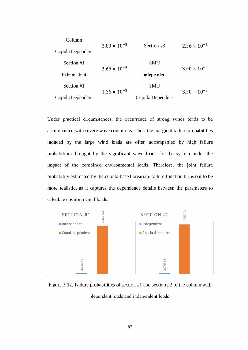
87

Column

Copula Dependent 2.80 × 10−3 Section #3 2.26 × 10−5

Section #1

Independent 2.66 × 10−5

SMU

Independent 3.00 × 10−4

Section #1

Copula Dependent 1.36 × 10−3

SMU

Copula Dependent 3.20 × 10−3

Under practical circumstances, the occurrence of strong winds tends to be

accompanied with severe wave conditions. Thus, the marginal failure probabilities

induced by the large wind loads are often accompanied by high failure

probabilities brought by the significant wave loads for the system under the

impact of the combined environmental loads. Therefore, the joint failure

probability estimated by the copula-based bivariate failure function turns out to be

more realistic, as it captures the dependence details between the parameters to

calculate environmental loads.

Figure 3-12. Failure probabilities of section #1 and section #2 of the column with

dependent loads and independent loads

2.6

6E-

05

1.3

6E-

03

SECTION #1

Independent

Copula dependent

2.7

7E-

05

1.4

2E-

03

SECTION #2

Independent

Copula dependent

88

On the other hand, Figure 3-10 and the selected Gumbel copula show the upper

tail dependence character. This clearly shows that the stronger wind speed and

higher wave height have more substantial dependence. On the basis of the copula-

based bivariate failure function in Equation (3.13), the larger the dependency, the

greater the value of the failure probability. Therefore, it is vital to take dependence

into consideration in extreme weather conditions.

In conclusion, consideration of the dependence structure between the parameters

to calculate the environmental loads for operational failure assessment is

necessary for the sake of safety production, especially in harsh environments. It

allows the failure probability to be much closer to reality. If feasible, it is

recommended that the historical wave and meteorological data of the operational

location be thoroughly investigated.

Conclusions 3.5

This paper proposes a novel methodology and robust model that consider real-

time weather observation and estimate the operational failure probability of the

system. The methodology is explained with a simple example. The developed

robust model is tested and applied to a detailed case study. The novelty of this

paper is the consideration of dependence between the parameters to calculate

environmental loads. The dependence is considered using the copula-based

bivariate failure function. The dependence parameters are estimated by

maximizing the pseudo log-likelihood functions. The selection of the best model

among all candidate copula models is accomplished with the aid of Akaike’s

89

information criterion (AIC). AIC differences and Akaike weight measure the

distances between the best model and candidate model and the level of empirical

support.

The comparison of the proposed approach with the traditional approach

considering independence demonstrates the advantage of the operational failure

assessment model considering the copula function. The failure probability

considering dependent loads calculated by the copula-based bivariate failure

function is noticeably higher and closer to the real-life situation. This observation

emphasizes the vital significance of considering dependence when defining safe

operation envelopes under extreme weather conditions. This work will help

decision-makers make informed operational decisions for the system.

It is important to note that one copula may not define all environmental parameter

conditions. The accuracy of copula selection strongly depends on the set of data

(in terms of the frequency and broader range). It is recommended that a proper

copula function be defined considering a wide range of data so both temporal and

spatial variations are captured in defining the dependency.

90

References 3.6

[1] Beven, J. L., Avila, L. A., Blake, E. S., Brown, D. P., Franklin, J. L., Knabb, R.

D., ... & Stewart, S. R. (2007). Annual summary: Atlantic hurricane season

of 2005. Monthly Weather Review, 136, 1109-1173.

[2] Cruz, A. M., & Krausmann, E. (2008). Damage to offshore oil and gas

facilities following hurricanes Katrina and Rita: An overview. Journal of

Loss Prevention in the Process Industries, 21(6), 620-626.

[3] DNVGL-RP-C205, Enviromental conditions and enviromental loads. August

2017. DNV GL

[4] American Bureau of Shipping (ABS), Rules for building and Classing Mobile

Offshore Drilling Units. 2019

[5] Suja-Thauvin, L., Krokstad, J. R., & Bachynski, E. E. (2018). Critical

assessment of non-linear hydrodynamic load models for a fully flexible

monopile offshore wind turbine. Ocean Engineering, 164, 87-104.

[6] Caille, F, Bozonnet, P, Melis, C, Poirette, Y, Perdrizet, P (2017). Model test

and simulation comparison for an inclined-leg TLP dedicated to floating

wind. Paper Presented at the ASME 2017 36th International Conference

on Ocean, Offshore and Arctic Engineering. San Francisco, CA, USA,

[7] Flis, L. (2016). Application of the rules of the American Bureau of Shipping

(ABS) to design mobile offshore structures. Scientific Journal of Polish

Naval Academy, 205(2), 17-28.

[8] Li, D. J., Fu, Q., Du, Z. F., Xiao, Y., Han, R. G., & Sun, H. H. (2018).

Structural Configuration Selection and Optimization of 7th Generation

Semi-Submersible Drilling Unit. Paper presented at the ASME 2018 37th

91

International Conference on Ocean, Offshore and Arctic Engineering.

Madrid, Spain.

[9] Durante, F., Sempi, C. (2015), Principles of Copula Theory, CRC Press, Boca

Raton, FL.

[10] Jia, X., Xing, L., & Li, G. (2018). Copula‐based reliability and safety

analysis of safety‐critical systems with dependent failures. Quality and

Reliability Engineering International, 34(5), 928-938.

[11] Zhang, X., & Wilson, A. (2017). System reliability and component

importance under dependence: A copula approach. Technometrics, 59(2),

215-224.

[12] Hashemi, S. J., Ahmed, S., & Khan, F. (2015). Operational loss modelling

for process facilities using multivariate loss functions. Chemical

Engineering Research and Design, 104, 333-345.

[13] Guo, C., Khan, F., & Imtiaz, S. (2019). Copula-based Bayesian network

model for process system risk assessment. Process Safety and

Environmental Protection, 123, 317-326.

[14] Shen, L., Zhang, Y., & Zhuang, X. (2016). Research on Function Reliability

of Gear Door Lock System with Correlated Failure Models Based on

Mixed Copula. Paper Presented at the ASME 2016 International

Mechanical Engineering Congress and Exposition. American Society of

Mechanical Engineers. Phoenix, Arizona, USA.

[15] Department of Fisheries and Oceans Canada (DFO). Wave data available on-

line. Available online: http://isdm-gdsi.gc.ca/isdm-gdsi/waves-

vagues/data-donnes/data-donnees-eng.asp?medsid=C44139.(accessed on

92

05 September 2019).

[16] Sklar, M. (1959). Fonctions de repartition an dimensions et leurs

marges. Publ. inst. statist. univ. Paris, 8, 229-231.

[17] Nelsen, R.b., (2006). An introduction to Copulas, second ed. Springer, New

York, NY.

[18] Melo, R., Accioly, S., & Aiube, F. A. L. (2008). Analysis of crude oil and

gasoline prices through copulas. Cadernos do IME-Série Estatística, 24(1),

15.

[19] Genest, C., & Favre, A. C. (2007). Everything you always wanted to know

about copula modeling but were afraid to ask. Journal of hydrologic

engineering, 12(4), 347-368.

[20] MathWorks, 2017. MATLAB Release 2017b. The MathWorks, Inc., Natick,

Massachusetts, United States.

[21] Burnham, K. P., Anderson, D. R., (2002). Model Selection and Multi-Model

Inference: A Practical Information-Theoretic Approach, 2nded. Springer,

Secaucus, NJ, USA.

[22] Ebeling CE. (1997) An Introduction to Reliability and Maintainability

Engineering.2nd ed. New Delhi: McGraw Hill;

[23] DNVGL-OS-C101, Design of offshore steel structures, general - LRFD

method. July 2019. DNV GL

[24] Zhang, S. (2017, August 25). When a hurricane hits an offshore oil platform:

Harvey could seriously damage oil and gas operations in the Gulf of

Mexico. The Atlantic: Science Edition. Retrieved from:

https://www.theatlantic.com /science/archive/2017/08/harvey-offshore-

93

platform-oil-gas/537960/

[25] Yuan, Z., Khakzad, N., Khan, F., & Amyotte, P. (2015). Risk analysis of dust

explosion scenarios using Bayesian networks. Risk analysis, 35(2), 278-

291.

[26] Fu, J., & Khan, F. (2019). Operational failure model for semi-submersible

mobile units in harsh environments. Ocean Engineering, 191, 106332.

94

Chapter 4. Summary

Keeping the safety operation of the offshore facilities in the harsh environment is

the top priority in meeting the growing demand for energy. Therefore, this thesis

proposes two related methodologies that assess the operational risk quantitatively

with combined environmental loads considering the dependence structure between

the real-time environmental parameters.

Chapter 1 introduces the overview of the current models that are employed to

capture the dynamic response of the offshore facilities under extreme weather

conditions and researchers’ application using related standards recommended by

classification societies to calculate environmental loads.

Chapter 2 presents a novel model that defines the operational failure envelope for

decision-makers’ reference which applies the weather condition and physical

characteristics of the offshore facilities.

Chapter 3 proposes a robust copula-based bivariate operational failure assessment

model which aims to explore the influence of the dependence function among

parameters to calculate the environmental loads.

Chapter 4 concludes the research, illustrates the novelty and highlights the

contribution of the developed methodologies. In the end, further recommendations

and future work are presented here for the sake of improvement.

Conclusions 4.1

Previous popular evaluation indicators mainly focus on either external

hydrodynamic performance or internal structure dynamic analysis instead of

quantitatively analyzing the operational risk. Furthermore, the dependencies

among parameters to calculate environmental loads are ignored which

95

underestimates the impact on the failure of the system. Therefore, this work fills

in the research gaps by assessing the operational risk quantitatively with combined

environmental loads which consider the dependency function.

The physical reliability model and the BN are used for the operational failure

model which is verified with a catastrophe capsizing accident - the Ocean Ranger

as a case application. The proposed model applies the weather conditions on-site

and the unit configuration and estimates a very high probability of failure which

predicts a dangerous prevailing situation. The occurrence of the fateful event

confirms the accuracy and effectiveness. It is demonstrated that the proposed

anticipated risk estimation model is a reliable tool to develop and monitor an

operational failure envelope of the SMU in given environmental conditions.

The copula-based bivariate operational failure assessment model is validated by a

typical semi-submersible mobile unit (SMU) operating in the Grand Banks with

the obtained wave and concurrent meteorological observation data from the buoy:

Banquereau – 44139. The comparison study of the proposed approach with the

traditional approach considering independence demonstrates the advantage of the

operational failure assessment model which takes the copula function into account.

The obvious differences indicate that the proposed model which captures the

dependence details among parameters to calculate the environmental loads is able

to better guide policy-makers for safety operational decisions.

Recommendation 4.2

It is worth mentioning that the environmental loads acting on the offshore

facilities are not only limited to the wind and wave loads under the practical

situation. More complicated and considerable cases such as currents and sea ice

96

induced loads should be taken into consideration to extend the operational

disturbance to a broader scope of contexts.

The following aspects for further research can achieve a deeper insight into the

copula-based bivariate failure model. It is important to note that the accuracy and

precision of copula selection strongly depend on the data set. The broader range

the data sets, the more the dependence details can be reflected. It is recommended

that the proper copula function be defined considering a wide range of data, so

both temporal and spatial variations are captured in defining the dependency.

Therefore, the further research direction is to determine the suitable copula

function facing the widely encountered issue of data paucity.