DYNAMIC NEURAL NETWORK-BASED ROBUST CONTROL …ncr.mae.ufl.edu/dissertations/huyen.pdf · dynamic...

DYNAMIC NEURAL NETWORK-BASED ROBUST CONTROL METHODS FOR

UNCERTAIN NONLINEAR SYSTEMS

By

HUYEN T. DINH

A DISSERTATION PRESENTED TO THE GRADUATE SCHOOL

OF THE UNIVERSITY OF FLORIDA IN PARTIAL FULFILLMENT

OF THE REQUIREMENTS FOR THE DEGREE OF

DOCTOR OF PHILOSOPHY

UNIVERSITY OF FLORIDA

2012

© 2012 Huyen T. Dinh

2

To my beautiful daughter Anh Tran, my loving husband Thong Tran, and my dear parents Hop

Pham and Tung Dinh, for their unwavering support and constant encouragement

3

ACKNOWLEDGMENTS

I would like to express my deepest gratitude to my advisor, Dr. Warren E. Dixon, for his

excellent guidance, caring, patience and support in the four years of my doctoral study. As an

advisor, he exposed me to the vast and exciting research area of nonlinear control and motivated

me to work on Dynamic Neural Network-based control applications. He encouraged me to

explore my own ideas and helped me grow as an independent researcher. I highly appreciate all

his caring and support as an understanding boss during my maternity time.

I would like to extend my gratitude to my committee members, Dr. Prabir Barooah, Dr.

Joshep Wilson, and Dr. Mrinal Kumar, for insightful comments and many valuable suggestions

to improve the presentation and contents of this dissertation.

I would also like to thank all my coworkers at the Nonlinear Controls and Robotics Lab for

their various forms of support during my graduate study. Their warm friendship has enriched my

life.

From the bottom of my heart, I would like to thank my parents for their support and belief in

me. Without their support, encouragement and unconditional love, I would never be able to finish

my dissertation. Also, I would like to thank and apologize to my daughter, who was born before

this dissertation was completed and spend most of her time with my mother to allow me to focus.

I am deeply sorry for the time we spend apart. Finally, I would like to thank my husband for his

constant patience and unwavering love.

4

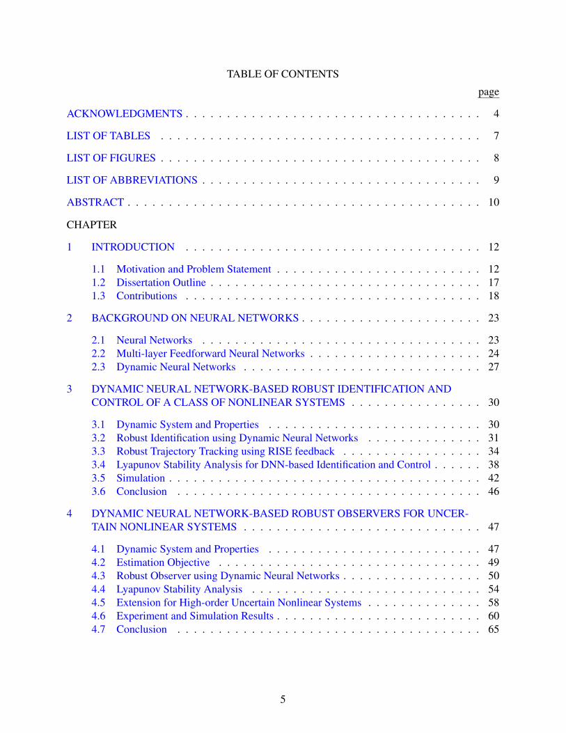
TABLE OF CONTENTS

page

ACKNOWLEDGMENTS . . . . . . . . . . . . . . . . . . . . . . . . . . . . . . . . . . . . 4

LIST OF TABLES . . . . . . . . . . . . . . . . . . . . . . . . . . . . . . . . . . . . . . . 7

LIST OF FIGURES . . . . . . . . . . . . . . . . . . . . . . . . . . . . . . . . . . . . . . . 8

LIST OF ABBREVIATIONS . . . . . . . . . . . . . . . . . . . . . . . . . . . . . . . . . . 9

ABSTRACT . . . . . . . . . . . . . . . . . . . . . . . . . . . . . . . . . . . . . . . . . . . 10

CHAPTER

1 INTRODUCTION . . . . . . . . . . . . . . . . . . . . . . . . . . . . . . . . . . . . 12

1.1 Motivation and Problem Statement . . . . . . . . . . . . . . . . . . . . . . . . . 12

1.2 Dissertation Outline . . . . . . . . . . . . . . . . . . . . . . . . . . . . . . . . . 17

1.3 Contributions . . . . . . . . . . . . . . . . . . . . . . . . . . . . . . . . . . . . 18

2 BACKGROUND ON NEURAL NETWORKS . . . . . . . . . . . . . . . . . . . . . . 23

2.1 Neural Networks . . . . . . . . . . . . . . . . . . . . . . . . . . . . . . . . . . 23

2.2 Multi-layer Feedforward Neural Networks . . . . . . . . . . . . . . . . . . . . . 24

2.3 Dynamic Neural Networks . . . . . . . . . . . . . . . . . . . . . . . . . . . . . 27

3 DYNAMIC NEURAL NETWORK-BASED ROBUST IDENTIFICATION AND

CONTROL OF A CLASS OF NONLINEAR SYSTEMS . . . . . . . . . . . . . . . . 30

3.1 Dynamic System and Properties . . . . . . . . . . . . . . . . . . . . . . . . . . 30

3.2 Robust Identification using Dynamic Neural Networks . . . . . . . . . . . . . . 31

3.3 Robust Trajectory Tracking using RISE feedback . . . . . . . . . . . . . . . . . 34

3.4 Lyapunov Stability Analysis for DNN-based Identification and Control . . . . . . 38

3.5 Simulation . . . . . . . . . . . . . . . . . . . . . . . . . . . . . . . . . . . . . . 42

3.6 Conclusion . . . . . . . . . . . . . . . . . . . . . . . . . . . . . . . . . . . . . 46

4 DYNAMIC NEURAL NETWORK-BASED ROBUST OBSERVERS FOR UNCER-

TAIN NONLINEAR SYSTEMS . . . . . . . . . . . . . . . . . . . . . . . . . . . . . 47


4.2 Estimation Objective . . . . . . . . . . . . . . . . . . . . . . . . . . . . . . . . 49

4.3 Robust Observer using Dynamic Neural Networks . . . . . . . . . . . . . . . . . 50

4.4 Lyapunov Stability Analysis . . . . . . . . . . . . . . . . . . . . . . . . . . . . 54

4.5 Extension for High-order Uncertain Nonlinear Systems . . . . . . . . . . . . . . 58

4.6 Experiment and Simulation Results . . . . . . . . . . . . . . . . . . . . . . . . . 60

4.7 Conclusion . . . . . . . . . . . . . . . . . . . . . . . . . . . . . . . . . . . . . 65

5

5 GLOBAL OUTPUT FEEDBACK TRACKING CONTROL FOR UNCERTAIN SECOND-

ODER NONLINEAR SYSTEMS . . . . . . . . . . . . . . . . . . . . . . . . . . . . 67


5.2 Estimation and Control Objectives . . . . . . . . . . . . . . . . . . . . . . . . . 68

5.3 DNN-based Robust Observer . . . . . . . . . . . . . . . . . . . . . . . . . . . . 69

5.4 Robust Adaptive Tracking Controller . . . . . . . . . . . . . . . . . . . . . . . . 72

5.5 Lyapunov Stability Analysis for DNN-based Observation and Control . . . . . . 75

5.6 Experiment Results . . . . . . . . . . . . . . . . . . . . . . . . . . . . . . . . . 78

5.7 Conclusion . . . . . . . . . . . . . . . . . . . . . . . . . . . . . . . . . . . . . 79

6 OUTPUT FEEDBACK CONTROL FOR AN UNCERTAIN NONLINEAR SYS-

TEMWITH SLOWLY VARYING INPUT DELAY . . . . . . . . . . . . . . . . . . . 82


6.2 Estimation and Control Objectives . . . . . . . . . . . . . . . . . . . . . . . . . 83

6.3 Robust DNN Observer Development . . . . . . . . . . . . . . . . . . . . . . . . 84

6.4 Robust Tracking Control Development . . . . . . . . . . . . . . . . . . . . . . . 86

6.5 Lyapunov Stability Analysis for DNN-based Observation and Control . . . . . . 88

6.6 Simulation Results . . . . . . . . . . . . . . . . . . . . . . . . . . . . . . . . . 93

6.7 Conclusion . . . . . . . . . . . . . . . . . . . . . . . . . . . . . . . . . . . . . 95

7 CONCLUSION AND FUTURE WORKS . . . . . . . . . . . . . . . . . . . . . . . . 97

7.1 Dissertation Summary . . . . . . . . . . . . . . . . . . . . . . . . . . . . . . . . 97

7.2 Future Work . . . . . . . . . . . . . . . . . . . . . . . . . . . . . . . . . . . . . 99

APPENDIX

A DYNAMIC NEURAL NETWORK-BASED ROBUST IDENTIFICATION AND

CONTROL OF A CLASS OF NONLINEAR SYSTEMS . . . . . . . . . . . . . . . . 101

A.1 Proof of the Inequality in Eq. (3–12) . . . . . . . . . . . . . . . . . . . . . . . . 101


A.3 Proof of the Inequality in Eqs. (3–25) and (3–26) . . . . . . . . . . . . . . . . . 102


B DYNAMIC NEURAL NETWORK-BASED GLOBAL OUTPUT FEEDBACK TRACK-

ING CONTROL FOR UNCERTAIN SECOND-ODER NONLINEAR SYSTEMS . . . 105

REFERENCES . . . . . . . . . . . . . . . . . . . . . . . . . . . . . . . . . . . . . . . . . 107

BIOGRAPHICAL SKETCH . . . . . . . . . . . . . . . . . . . . . . . . . . . . . . . . . . 114

6

LIST OF TABLES

Table page

4-1 Transient (t = 0− 1 sec) and steady state (t = 1− 10 sec) velocity estimation errors˙x(t) for different velocity estimation methods in presence of noise 50dB. . . . . . . . . 65

5-1 Steady-state RMS errors and torques for each of the analyzed control designs. . . . . . 79

6-1 Link1 and Link 2 RMS tracking errors and RMS estimation errors. . . . . . . . . . . . 95

6-2 RMS errors for cases of uncertainty in time-varying delay seen by the plant as com-

pared to the delay of the controller. . . . . . . . . . . . . . . . . . . . . . . . . . . . . 95

7

LIST OF FIGURES

Figure page

2-1 Nonlinear model of a neuron . . . . . . . . . . . . . . . . . . . . . . . . . . . . . . . 24

2-2 Two-layer NN . . . . . . . . . . . . . . . . . . . . . . . . . . . . . . . . . . . . . . 25

2-3 Hopfield DNN circuit structure . . . . . . . . . . . . . . . . . . . . . . . . . . . . . . 27

3-1 The architecture of the MLDNN. . . . . . . . . . . . . . . . . . . . . . . . . . . . . . 32

3-2 Robust identification-based trajectory tracking control. . . . . . . . . . . . . . . . . . 36

3-3 Link 1 and link 2 tracking errors. . . . . . . . . . . . . . . . . . . . . . . . . . . . . . 44

3-4 Link 1 and Link 2 position identification errors. . . . . . . . . . . . . . . . . . . . . . 44

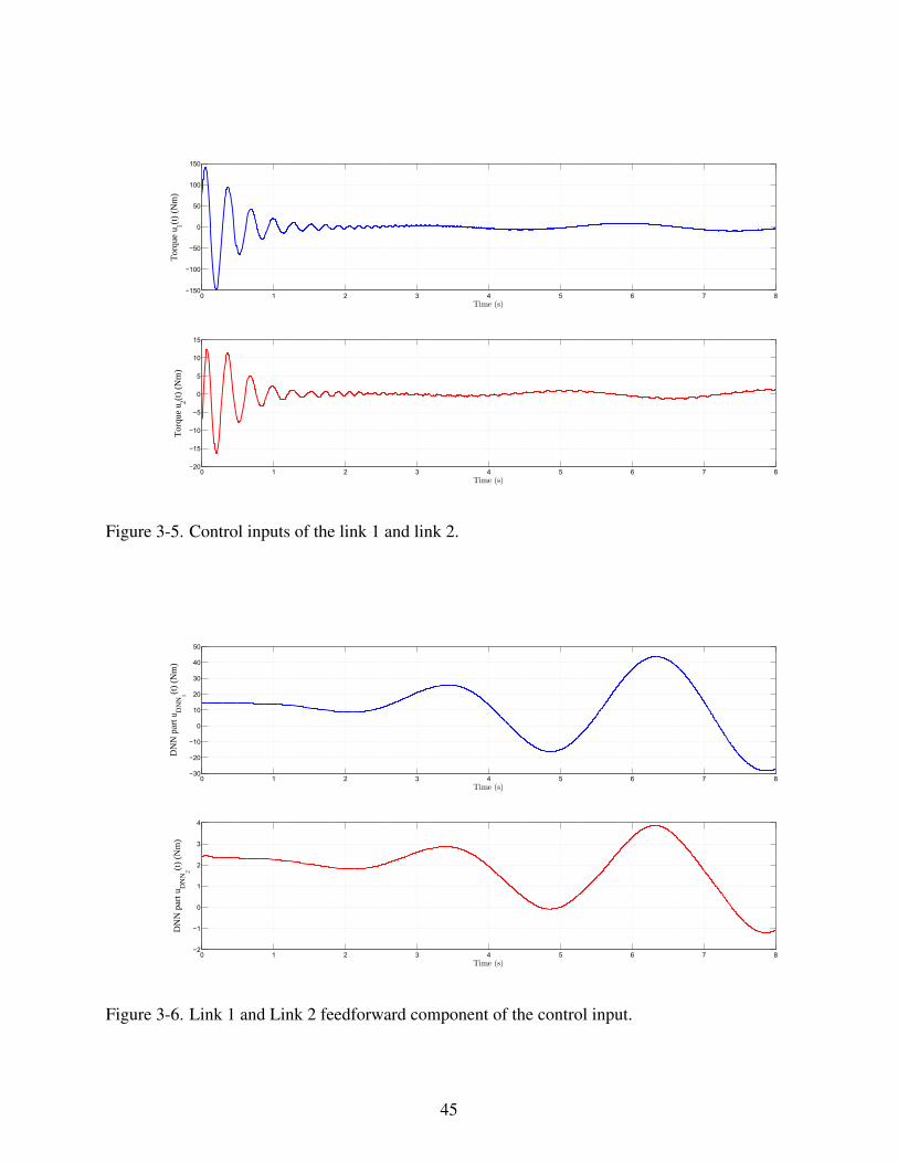
3-5 Control inputs of the link 1 and link 2. . . . . . . . . . . . . . . . . . . . . . . . . . . 45

3-6 Link 1 and Link 2 feedforward component of the control input. . . . . . . . . . . . . . 45

4-1 The experimental testbed consists of a two-link robot. The links are mounted on two

NSK direct-drive switched reluctance motors. . . . . . . . . . . . . . . . . . . . . . . 60

4-2 Velocity estimate ˙x(t) using (a) [1], (b) [2], (c) the proposed method, and (d) the cen-ter difference method on a two-link experiment testbed. . . . . . . . . . . . . . . . . 62

4-3 The steady-state velocity estimate ˙x(t) using (a) [1], (b) [2], (c) the proposed method,and (d) the center difference method on a two-link experiment testbed. . . . . . . . . . 63

4-4 Frequency analysis of velocity estimation ˙x(t) using (a) [1], (b) [2], (c) the proposedmethod, and (d) the center difference method on a two-link experiment testbed. . . . . 63

4-5 The steady-state velocity estimation error ˙x(t) using (a) [1], (b) [2], (c) the proposedmethod, and (d) the center difference method on simulations, in presence of sensor

noise (SNR 60dB). The right figures (e)-(h) indicate the respective frequency analysis

of velocity estimation ˙x(t). . . . . . . . . . . . . . . . . . . . . . . . . . . . . . . . . 65

5-1 The tracking errors e(t) of (a) Link 1 and (b) Link 2 using classical PID, robust dis-continuous OFB controller [1], and proposed controller. . . . . . . . . . . . . . . . . . 79

5-2 Control inputs for Link 1 and Link 2 using (a), (b) classical PID, (c), (d) robust dis-

continuous OFB controller [1], and (e), (f) the proposed controller. . . . . . . . . . . . 80

5-3 Velocity estimation x(t) using (a) DNN-based observer and (b) numerical backwardsdifference. . . . . . . . . . . . . . . . . . . . . . . . . . . . . . . . . . . . . . . . . . 81

6-1 Simulation results with 10% magnitude and 10% offset variance in time-delay . . . . . 96

8

LIST OF ABBREVIATIONS

DNN Dynamic Neural Network

LK Lyapunov-Krasovskii

LP Linear-in-parameter

MLNN Multi-layer Neural Network

NN Neural Network

OFB Output Feedback

RISE Robust Integral of the Sign of the Error

RMS Root Mean Squares

UUB Uniformly Ultimately Bounded

9

Abstract of Dissertation Presented to the Graduate School

of the University of Florida in Partial Fulfillment of the

Requirements for the Degree of Doctor of Philosophy

DYNAMIC NEURAL NETWORK-BASED ROBUST CONTROL METHODS FOR

UNCERTAIN NONLINEAR SYSTEMS

By

Huyen T. Dinh

August 2012

Chair: Warren E. Dixon

Major: Mechanical Engineering

Neural networks (NNs) have proven to be effective tools for identification, estimation and

control of complex uncertain nonlinear systems. As a natural extension of feedforward NNs

with the capability to approximate nonlinear functions, dynamic neural networks (DNNs) can

be used to approximate the behavior of dynamic systems. DNNs distinguish themselves from

static feedforward NNs in that they have at least one feedback loop and their representation is

described by differential equations. Because of internal state feedback, DNNs are known to

provide faster learning and exhibit improved computational capability in comparison to static

feedforward NNs.

In this dissertation, a DNN architecture is utilized to approximate uncertain nonlinear

systems as a means to develop identification methods and observers for estimation and control.

In Chapter 3, an identification-based control method is presented, wherein a multilayer DNN

is used in conjunction with a sliding mode term to approximate the input-output behavior of a

plant while simultaneously tracking a desired trajectory. This result is achieved by combining

the DNN-identification strategy with a RISE (Robust Integral of the Sign of the Error) controller.

In Chapters 4 and 5, a class of second-order uncertain nonlinear systems with partially unmea-

surable states is considered. A DNN-based observer is developed to estimate the missing states

in Chapter 4, and the DNN-based observer is developed for an output feedback (OFB) tracking

control method in Chapter 5. In Chapter 6, an OFB control method is developed for uncertain

nonlinear systems with time-varying input delays. In all developed approaches, weights of the

10

DNN can be adjusted on-line: no off-line weight update phase is required. Chapter 7 concludes

the proposal by summarizing the work and discussing some future problems that could be further

investigated.

11

CHAPTER 1

INTRODUCTION

1.1 Motivation and Problem Statement

Based on their approximation properties, NNs have proven to be effective tools for identifi-

cation, estimation and control of complex uncertain nonlinear systems. Feedforward NNs have

been extensively used for adaptive control: NNs are cascaded into the controlled system and the

NN weights are directly adjusted through an adaptive update law that is a function of the tracking

error [3–5]. Contrary to feedforward NNs, the neurons of DNNs receive not only external input

(e.g., tracking error) but also internal state feedback. Feedforward and feedback connections al-

low information in DNNs to propagate in two directions: from input neurons to outputs and vice

versa [6]. Since DNNs exhibit dynamic behavior, they can be used as dynamic models to repre-

sent nonlinear systems, unlike feedforward NNs which can only approximate nonlinear functions

in a system. From a computational perspective, a DNN with state feedback may provide more

computational advantages than a static feedforward NN [7]. Funahashi and Nakamura [8] and

Polycarpou [9] proved that DNNs could approximate the input-output behavior of a plant with

arbitrary accuracy.

Narendra [10] proposed the idea of using DNNs for identification of nonlinear systems,

wherein the identification models (DNNs) have the same structure as the plant but contain

NNs with adjustable weights. The DNN-based learning paradigm involves the identification

of the input-output behavior of the plant and the use of the resulting identification model to

adjust the parameters of the controller [10]. In [11], recurrent higher order NNs are used for

identification of nonlinear systems, where the dynamical neurons are distributed throughout

the network. Rovithakis and Christodoulou [12] used singular perturbation to investigate the

stability and robustness properties of the DNN identifier, and designed a state feedback law to

track a reference model. In [13], a Hopfield-type DNN is used to identify a single input/single

output (SISO) system, and the identifier is used in the controller to feedback linearize the system,

which is then controlled using a PID controller. Poznyak used a parallel Hopfield-type NN for

12

identification and trajectory tracking [14, 15] and proved bounded Lyapunov stability of the

identification and tracking errors in presence of modeling errors. Ren et al. [16] proposed a

DNN structure for identification and control of nonlinear systems by using just the input/output

measurements. The Hopfield-type DNN is widely used because of its simple structure and

desirable stability properties [7, 17]. However, its structure only includes the single-layer NN,

so its approximation capability is limited in comparison with a multi-layer DNN. A multi-layer

DNN with stable learning laws is used in [18] for nonlinear system identification. However,

all of the previous DNN methods are limited to uniformly ultimately bounded results, because

of the residual function approximation error. In contrast, Chapter 3 proposes a modified DNN

identifier structure to prove that the identification error is asymptotically regulated with only

typical gradient weight update laws, and a controller including a DNN-identifier term and a

robust feedback term (RISE) is used to ensure asymptotic tracking of the system along a desired

trajectory. Both asymptotic identification and asymptotic tracking are achieved simultaneously

while the DNN weights are adapted on-line.

Typical identification-based control approaches [12, 16, 19, 20] require the system states

to be completely measurable. However, full state feedback is not always available in many

practical systems. In the absence of sensors, the requirement of full-state feedback for the

controller is typically fulfilled by using ad hoc numerical differentiation techniques, which can

aggravate the problem of noise, leading to unusable state estimates. Several nonlinear observers

are proposed in literature to estimate unmeasurable states. For instance, sliding mode observers

were designed for general nonlinear systems by Slotine et al. in [21], for robot manipulators

by Canudas de Wit et al. in [22], and for mechanical systems subject to impacts by Mohamed

et al. in [23]. However, all these observers require exact model knowledge to compensate for

nonlinearities in the system. Model-based observers are also proposed in [24] and [25] which

require a high-gain to guarantee convergence of the estimation error to zero. The observers

introduced in [26] and [27] are both applied for Lagrangian dynamic systems to estimate the

velocity, and asymptotic convergence to the true velocity is obtained. However, the symmetric

13

positive-definiteness of the inertia matrix and the skew-symmetric property of the Coriolis matrix

are required. Model knowledge is required in [26] and a partial differential equation needs

to be solved to compute the observers. In [27], the system dynamics must be expressed in a

non-minimal model and only mass and inertia parameters are unknown in the system.

The design of robust observers for uncertain nonlinear systems is considered in [1, 28, 29].

In [28], a second-order sliding mode observer for uncertain systems using a super-twisting

algorithm is developed, where a nominal model of the system is assumed to be available and

estimation errors are proven to converge in finite-time to a bounded set around the origin.

In [29], the proposed observer can guarantee that the state estimates converge exponentially

fast to the actual state, if there exists a vector function satisfying a complex set of matching

conditions. In [1], one of the first asymptotic velocity observers is developed for general second-

order systems, where the estimation error is proven to asymptotically converge. However,

all nonlinear uncertainties in [1] are damped out by a sliding mode term resulting in high

frequency state estimates. A NN approach that uses the universal approximation property is

investigated for use in an adaptive observer design in [30]. However, estimation errors in [30]

are only guaranteed to be bounded due to function reconstruction inaccuracies. Inspired by [1]

and [30], a robust adaptive DNN-based observer is introduced in Chapter 4, where the DNN

is used to approximate the uncertain system, a dynamic filter works in junction with the DNN

to reconstruct the unmeasurable state, and a sliding mode term is added to the observer to

compensate for the approximation error and exogenous disturbance. Asymptotic estimation is

proven by a Lyapunov-based stability analysis and illustrated by experiments and simulations.

In addition to OFB observers, various OFB controllers have also been developed. OFB

controllers using model-based observers were developed in [31–33]. In [31], Berghuis et al.

designed an observer and a controller for robot models using a passivity approach for both

positioning and tracking objectives based on the condition that the system dynamics are exactly

known. Do et al. in [32] considered observer-based OFB control for unicycle-type mobile

robots to stabilize the system and track a desired trajectory. In [33], a controller based on an

14

observer-based integrator backstepping technique was proposed for a revolute manipulator with

known dynamics, and a semi-global exponential stability result for the link position tracking

error and the velocity observation error was achieved. A disadvantage of these approaches is the

requirement of exact model knowledge. OFB control for systems with parametric uncertainties

has been developed in [34–37]. A linear observer is used in [34] to estimate the angular velocity

of a rigid robot arm which is required to satisfy the linear-in-parameters (LP) condition, and

uniform ultimate boundedness of the tracking and observation errors is obtained. Adaptive

OFB control for robot manipulators satisfying the LP condition which achieves semi-global

asymptotic tracking results is considered in [35–37]. The difference between these approaches

is the joint velocity is estimated by an observer in [35], while a filter is used for velocity

estimation in [36] and [37]. An extension of [36] and [37] to obtain a global asymptotic tracking

result was introduced in [38]. However, a limitation of such previous adaptive OFB control

approaches is that only LP uncertainties are considered. As a result, if uncertainties in the system

do not satisfy the LP condition or if the system is affected by disturbances, the results will

reduce to a uniformly ultimately bounded (UUB) result. The condition of linear dependence

upon unknown parameters can be relaxed by introducing a NN or fuzzy logic in the observer

structure as in [30, 39–43]; however, both estimation and tracking errors are only guaranteed

to be bounded due to the existence of reconstruction errors. The first semi-global asymptotic

OFB tracking result for second-order dynamic systems under the condition that uncertain

dynamics are first-order differentiable was introduced in [1] with a novel filter design. All of

the uncertain nonlinearities in [1] are damped out by a sliding mode term, so the discontinuous

controller requires high-gain. The OFB control approach in Chapter 5 is motivated by [1] and the

observer design in Chapter 4. In this approach, the DNN-based observer is used to estimate the

unmeasurable state of the system; the controller, including the state estimation, NN, and sliding

mode terms are used to yield trajectory tracking. Both asymptotic estimation of the unmeasurable

state and asymptotic tracking of the desired trajectory are achieved simultaneously. Experiments

demonstrate the performance of the developed approach.

15

For many practical systems, time delay is inevitable. The torque generated by an internal

combustion engine can be delayed due to fuel-air mixing, ignition delays, cylinder pressure

force propagation (see, e.g., [44, 45]), or communication delays in remote control applications

where time is required to transmit information used for feedback control (see, e.g., master-slave

teleoperation of robot in [46–50]). Unfortunately, time delay is a source of instability and can

decrease system performance.

Delay in the control input (i.e, actuator delay) is an issue that has attracted significant

attention. Various stability analysis methods and control design techniques have been developed

for systems with input delays. For nonlinear systems, Lyapunov-Krasovskii (LK) functional-

based methods (cf. [51–53]) and Lyapunov-Razumikhin methods (cf. [54–56]) are the most

widely used tools to investigate the stability of a system affected by time delays. Compared with

frequency domain methods that check if all roots of the characteristic equation of a retarded or

neutral partial differential equation have negative real parts [57, 58], limiting its applicability

to only linear time-invariant systems with exact model knowledge, the Krasovskii-type and

Razumikhin-type approaches can be applied for uncertain nonlinear systems with time-varying

delays. Comparing between the Razumikhin-type and LK functional-type techniques reveals

that the Razumikhin methods can be considered as a particular but more conservative case of

Krasovskii methods, where Razumikhin methods can be applied to arbitrarily large, bounded

time-varying delays (0≤ τ(t)< ∞) , whereas the Krasovskii methods require a bounded

derivative of the delays (τ(t)≤ ϕ < 1). However, the Razumikhin approach requires input-to-

state stability of the nominal system without delay.

Various full-state feedback controllers have been developed that are based on LK or

Razumikhin stability criterion for nonlinear systems with input delays. Approaches in [59–63]

provide control methods for uncertain nonlinear systems with known and unknown constant

time-delays. However, time-delays are likely to vary in practice. Several methods for nonlinear

systems with time-varying input delays have been recently investigated. Linearized controllers

in [64, 65] are only valid within a region around the linearization point. A controller developed

16

in [66], which is an extension of [61, 67], deals with forward complete nonlinear systems with

time-varying input delay under an assumption that the plant is asymptotically stable in the

absence of the input delay. In [66], an invertible infinite dimensional backstepping transformation

is used to yield an asymptotically stable system. An Euler-Lagrange system with a slowly

varying input delay is considered in [68], where full state feedback is required. However, if only

system output is available for feedback, how to design a controller to handle both the lack of the

state and the time-varying delay of the input is rarely investigated. Studies in [69–71] address the

OFB control problem for nonlinear systems with constant input delay by linearization method. A

spacecraft, flexible-joint robot and rigid robot with constant time delay are considered in [69–71],

respectively, where the objectives are to design OFB controllers to stabilize the systems around

a set point. The controllers are first designed for delay-free linearized systems, then robustness

to the delay is proven provided certain delay dependent conditions hold true. To the author’s

knowledge, an OFB control method for nonlinear systems with time-varying input delay and

tracking control objectives is still an open problem.

1.2 Dissertation Outline

Chapter 1 serves as an introduction. The motivation, problem statement, literature review,

the contributions and the proposed research plan of the dissertation are discussed in this chapter.

Chapter 2 provides a background discussion on NNs, reviewing multi-layer neural network

(MLNN) and DNN structures, their learning laws, and their approximation properties.

Chapter 3 provides a methodology for DNN-based identification and tracking control.

The identifier structure is modified by adding a robust sliding mode term to account for the

reconstruction error, hence the input-output behavior of the identifier is proven to asymptotically

track the input-output behavior of the system. The controller, including information from the

identifier and the RISE feedback term is proposed to guarantee asymptotic tracking of the system

to the desired trajectory. The performance of the identification and control is illustrated through

simulations.

17

Chapter 4 illustrates a novel robust adaptive observer design for second-order uncertain non-

linear systems. The observer is designed based on a DNN to approximate the uncertain system,

a dynamic filter to provide a surrogate for the unmeasurable state, and a sliding mode term to

cancel out the approximation error and exogenous disturbance. The asymptotic estimation result

is proven by Lyapunov-based stability analysis and illustrated by experiments and simulations.

Chapter 5 develops an OFB control approach for second-order uncertain nonlinear systems,

where the DNN-based observer is used to estimate the unmeasurable state of the system and

the controller includes the state estimation, NN, and sliding mode terms to force the system to

track a desired trajectory. Both asymptotic estimation of the unmeasurable state and asymptotic

tracking of the desired trajectory are achieved simultaneously. Experiment results demonstrate

the performance of the developed approach.

Chapter 6 considers OFB control method for uncertain nonlinear systems affected by time-

varying input delays and additive disturbances. The delay is assumed to be bounded and slowly

varying. The DNN-based observer works in junction with the controller to provide an estimate

for the unmeasurable state. UUB estimation of the unmeasurable state and UUB tracking in the

presence of model uncertainty, disturbances, and time delays are proven by a Lyapunov-based

stability analysis.

Chapter 7 describes the possible directions that could extend the outcomes of the work in

this dissertation.

1.3 Contributions

The contributions in this dissertation are provided in Chapters 3-6.

Chapter 3: DNN-based robust identification and control of a class of nonlinear sys-

tems: The focus of this chapter is the development of an indirect control strategy (identification-

based control) for a class of uncertain nonlinear systems. A modified DNN structure is proposed

where a multi-layer DNN is combined with an identification error-based sliding mode term.

Unlike most DNN results which consider a single-layer Hopfield-type series-parallel configura-

tion of the DNN, this method considers a parallel multi-layer DNN configuration, which has the

18

advantage of providing better approximation accuracy [15]. The additional sliding mode term is

used to robustly account for exogenous bounded disturbances, modeling errors, and the function

reconstruction errors of the DNN. This modified DNN structure allows identification of uncertain

nonlinear systems while ensuring robustness to external disturbances. The idea of robust identifi-

cation of nonlinear systems was first proposed by Poznyak [72], who used a sliding mode term in

the algebraic weight update laws and ensured regulation of the identification error to zero. Huang

and Lewis [73] used a high gain robustifying term in the DNN structure to prove UUB stability

of nonlinear systems with time-delay. However, the proposed use of the sliding mode term in the

DNN structure is novel and advantageous since it provides robustness to matched disturbances

in the system without the need to modify the weight update laws. Asymptotic convergence of

the identification error is also guaranteed. The identifier is developed to facilitate the design of

the controller for the purpose of trajectory tracking. The controller consists of a DNN-identifier

term and a robust feedback term (RISE) [74, 75] to ensure asymptotic tracking of the system

along a desired trajectory. Asymptotic tracking is a contribution over previous results, where

only bounded stability of the tracking error could be proven due to the presence of modeling and

function reconstruction errors of the DNN. The use of the continuous RISE term is preferred

over the sliding mode term in the feedback controller to avoid chattering and other side-effects

associated with using a discontinuous control strategy. One of the assumptions in the use of the

RISE feedback technique is that the disturbance terms are bounded by known constants and their

derivatives be bounded by either a constant or a linear combination of the states. To satisfy these

boundedness assumptions, a bounded, user-defined sample state is introduced in the design of

the weight update laws for the DNN. No offline identification stage is required, and both the

controller and the identifier operate simultaneously in real-time.

Chapter 4: DNN-based robust observers for second-order uncertain nonlinear sys-

tems: The challenge to obtain asymptotic estimation stems from the fact that to robustly account

for disturbances, feedback of the unmeasurable error and its estimate are required. Typically,

feedback of the unmeasurable error is derived by taking the derivative of the measurable state

19

and manipulating the resulting dynamics (e.g., this is the approach used in methods such as [1]

and [30]). However, such an approach provides a linear feedback term of the unmeasurable state.

Hence, a sliding mode term could not be simply added to the NN structure of the result in [30]

to yield an asymptotic result, because it would require the signum of the unmeasurable state, and

it does not seem clear how this nonlinear function of the unmeasurable state can be injected in

the closed-loop error system using traditional methods. Likewise, it is not clear how to simply

add a NN-based feedforward estimation of the nonlinearities in results such as [1] because of

the need to inject nonlinear functions of the unmeasurable state. The novel approach used in this

chapter avoids this issue by using nonlinear (sliding mode) feedback of the measurable state, and

then exploiting the recurrent nature of a DNN structure to inject terms that cancel cross terms

associated with the unmeasurable state. The approach is facilitated by using the filter structure of

the controller in [1] and a novel stability analysis. The stability analysis is based on the idea of

segregating the nonlinear uncertainties into terms which can be upper-bounded by constants and

terms which can be upper-bounded by states. The terms upper-bounded by states can be canceled

by linear feedback of the measurable errors, while the terms upper-bounded by constants are

partially rejected by the sign feedback (of the measurable state) and partially eliminated by the

novel DNN-based weight update laws. The contribution of this chapter over previous results is

that the observer is designed for uncertain nonlinear systems, and the on-line approximation of

the unmeasurable uncertain nonlinearities via the DNN structure should heuristically improve

the performance of methods that only use high-gain feedback. Asymptotic convergence of

the estimated states to the real states is proven using a Lyapunov-based analysis for a general

second-order system. An extension of the proposed observer for a high-order system is shown,

whereas, the output of the nth order system is assumed to be measurable up to n− 1 derivatives.The developed observer can be used separately from the controller even if the relative degree

between the control input and the output is arbitrary. Simulation and experiment results on a

two-link robot manipulator show the effectiveness of the proposed observer when compared with

20

a standard numerical central differentiation algorithm, the high gain observer proposed in [2],

and the observer in [1].

Chapter 5: DNN-based global output feedback tracking control for second-order

uncertain nonlinear systems: In this chapter, a DNN-based observer-controller is proposed

for uncertain nonlinear systems affected by bounded external disturbances, to achieve a two-

fold result: asymptotic estimation of unmeasurable states and asymptotic tracking control.

Asymptotic estimation of unmeasurable states is exploited from DNN-based observer design

introduced in Chapter 4; however, asymptotic tracking is not simply obtained by replacing

the estimation state with the unmeasurable state in the control law. The challenge is that the

disturbances are again included in the open-loop tracking error system. To robustly account for

disturbances, both linear and nonlinear feedback of the unmeasurable tracking error are required.

The linear feedback is utilized from the linear feedback of unmeasurable estimation error, as

in Chapter 4. However, it is not clear how to inject the nonlinear feedback of the unmeasurable

tracking error from the measurable state and the estimation state. The approach used in Chapter 5

avoids this issue by using the sliding mode feedback of the measurable tracking error combined

with the novel stability analysis. A modified version of the filter introduced in [1] is used to

estimate the output derivative. Modification in the definition of the filtered estimation and

tracking errors is utilized. A combination of a NN feedforward term, along with estimated state

feedback and sliding mode terms are designed for the controller. The DNN observer adapts

on-line for nonlinear uncertainties and should heuristically perform better than a robust feedback

observer. New weight update laws for the DNN based on the estimation error, tracking error and

filter output are proposed. Asymptotic regulation of the estimation error and asymptotic tracking

are achieved.

Chapter 6: Output Feedback Control for an Uncertain Nonlinear System with

Slowly Varying Input Delay: The challenge to design an OFB control for uncertain nonlinear

systems with time-varying input delays stems from two questions: how to inject the negative

feedback of the state through the delayed input, and how to account for the delayed state which is

21

introduced into the closed-loop system by the input. Normally, with full-state feedback methods

as in [63, 68], the answer for the first question is the use of a predictor term which can provide a

free delay input to the system and the solution for the second question is the use of an auxiliary

LK functional, which is the integral over a delay time interval of the norm square of the state,

hence, the time derivative of the LK functional can provide a negative feedback term of the norm

square of the delayed state which itself cancels all state delay terms. However, with OFB control,

the difficulty is that the corresponding state is unmeasurable so it can not indirectly feedback into

the system via the predictor term. The approach to solve the issue in this chapter is motivated

from the use of a DNN-based observer in [76] and [77] to include a negative feedback of an

unmeasurable estimation error signal into the closed-loop system via a dynamic filter, then a

controller is designed based on the difference residual between the unmeasurable state with

the unmeasurable error signal, where this residual is measurable. Hence, finally through the

predictor term, the residual without delay is added to the closed-loop system along with the error

signal to form the negative feedback of the unmeasurable state. To deal with the delayed residual

injected to the system, similarly, an auxiliary LK functional including the norm square of the

residual term is used, then UUB tracking and estimation results are proven by Lyapunov-based

techniques.

In this chapter, an OFB control for a second-order uncertain nonlinear system with addi-

tive disturbances is developed to compensate for both the inaccessibility of all states and the

time-varying delay of the input. The delay is assumed to be bounded and slowly varying. A

DNN-based observer with on-line update algorithms is used to provide a surrogate for the un-

measurable state, a predictor term is utilized to inject a delay free control into the analysis, and

LK functionals are used to facilitate the design and stability analysis. The developed controller

achieves simultaneously UUB estimation of the unmeasurable state and UUB tracking results,

despite the lack of full state feedback, the time-varying input delay, uncertainties, and exogenous

disturbances in the plant dynamics. A numerical simulation for a two-link robot manipulator is

provided to examine the performance of the proposed method.

22

CHAPTER 2

BACKGROUND ON NEURAL NETWORKS

2.1 Neural Networks

In this chapter, a brief background on artificial NNs is provided. NN structures, learning

methods, and approximation properties are included. The structures of both multilayer NNs and

DNNs are described.

A NN is a massively parallel distributed processor composed of simple processing units that

have a natural propensity for storing experiential knowledge and making it available for use. A

NN resembles the brain in two respects [78]:

1. Knowledge is acquired by the network from its environment through a learning process.

2. Interneuron connection strengths, known as synaptic weights, are used to store the acquired

knowledge.

The procedure for the learning process is called a learning algorithm. Its function is to modify

the synaptic weights of the network to attain a desired design objective. The weight modification

equips the method for NN design and implementation. Facilitating identification, estimation,

and control for a wide class of nonlinear systems, NNs offer several useful properties and

capabilities:

1. NONLINEARITY. A NN is constructed from an interconnection of nonlinear neurons, so it

is itself nonlinear. This is an important property, especially if the underlying mechanism is

inherently nonlinear.

2. INPUT-OUTPUT MAPPING. The synaptic weights (free parameters) of the network are

modified to minimize the difference between the desired response and the actual response

of the network produced by the input signal in accordance with appropriate criterion.

Hence, the NN can adapt to construct the desired input - output mapping.

3. ADAPTIVITY. NNs have a built-in capability to adapt their weights based on design

criterion. The on-line learning algorithm can lead the network to adapt in real time.

23

Figure 2-1. Nonlinear model of a neuron

A neuron is the fundamental unit for the operation of a NN. Its model is shown in Fig. 2-1 with

three basic elements:

1. A set of synapses links, with each element characterized by its own weight,

2. An adder for summing the input signals multiplied by their respective weights,

3. A nonlinear activation function transforming the adder output into the output of the neuron.

In mathematical terms, the neuron can be described as

y j = σ

(n

∑i=1

wi jxi +b j

),

where x1, x2, ..., xn are the input signals, w1 j, w2 j, .., wn j are the respective synaptic weights of

neuron j, b j is the bias, σ(·) is the activation function, and y j is the output signal of the neuron.

The activation function σ(·) is often chosen as hard limit, linear threshold, sigmoid, hyperbolictangent, augmented ratio of squares, or radial basis functions.

The way in which neurons of a NN are interconnected determines its structure. In the

following, the structure for a multilayer feedforward neural network (MLNN) and the structure

for a DNN are considered.

2.2 Multi-layer Feedforward Neural Networks

Multi-layer feedforward NNs distinguishes itself by the presence of one or more hidden

layers in addition to input and output layers. The neurons in each layer have the output of the

preceding layer as their inputs. If each neuron in each layer is connected to every neuron in the

24

Figure 2-2. Two-layer NN

adjacent forward layer, then the NN is fully connected. The most common structure of MLNNs

is a two-layer NN, shown in Fig. 2-2.

A mathematical formula describing a two-layer NN is given by

yi =L

∑j=1

[wi jσ

(n

∑k=1

v jkxk +θv j

)+θwi

], i = 1,2, ...m.

The NN can be rewritten in matrix form as

y =W T σ(V T x),

where the output vector is y = [y1 y2 . . .ym]T ∈ R

m, the input vector is x = [1 x1 x2 . . .xn]T ∈ R

n+1,

the activation vector defined for a vector ξ = [ξ1 ξ2 . . .ξL]Tis σ(ξ ) = [1σ(ξ1)σ(ξ2) . . .σ(ξL)]

T ∈

25

RL+1, and the weight matricesW, V contain the thresholds in the first columns as

W =

⎡⎢⎢⎢⎢⎢⎢⎢⎣

θw1 w11 . . . w1L

θw2 w21 . . . w2L...

......

θwm wm1 . . . wmL

⎤⎥⎥⎥⎥⎥⎥⎥⎦

T

∈ R(L+1)×m, V =

⎡⎢⎢⎢⎢⎢⎢⎢⎣

θv1 v11 . . . v1n

θv2 v21 . . . v2n...

......

θvL vL1 . . . wLn

⎤⎥⎥⎥⎥⎥⎥⎥⎦

T

∈ R(n+1)×L.

The weights of NNs can be tuned by many techniques. A common weight-tuning algo-

rithm is the gradient algorithm based on the backpropagated error. A continuous version of

backpropagation tuning is given by

W = Γwσ(V T xd)ET , V = Γvxd(σ ′TWE)T ,

where Γw, Γv are the design gains, the backpropagated error E = yd − y, with yd ∈ Rm is the

desired NN output in response to the reference input xd ∈ Rn, and y ∈ R

m is the actual NN

output. The term σ ′(·) is the derivative of the activation function σ(·), which can be calculatedeasily. For example, if the activation function is chosen as the sigmoid function, the term σ ′(·) isequal to

σ ′ ≡ diag{

σ(V T xd)}[

I−diag{

σ(V T xd)}]

.

Approximation using two-layer NNs:

Let f (x) be a general smooth function from Rn to Rm. As long as x is restricted to a

compact set S of Rn, there exist NN weights and thresholds such that

f (x) =W T σ(V T x)+ ε,

for some number L of hidden-layer neurons. The universal function approximation property

holds for a large class of activation functions and the functional reconstruction error ε can be

made arbitrarily small by increasing the number of nodes in the network structure. Generally, ε

decreases as L increases. In fact, for any positive number εN , there exist weights and an L such

that ‖ε‖< εN , for all x ∈ S. Further details are provided in [78] and [46].

26

Figure 2-3. Hopfield DNN circuit structure

2.3 Dynamic Neural Networks

DNNs distinguish themselves from other types of NNs (static MLNNs) in that they have at

least one feedback loop. The feedback loops result in a nonlinear dynamical behavior of DNNs.

A DNN structure that contains state feedback may provide more computational advantages than

a static neural structure, which contains only a feedforward neural structure. In general, a small

feedback system is equivalent to a large and possibly infinite feedforward system [79]. A very

well known DNN structure is the Hopfield structure [17, 80], which can be implemented by

an electronic circuit. A continuous-time Hopfield DNN containing n units is described by the

following differential equations [7]:

State equation :Cidxi(t)

dt=−xi(t)

Ri+

n

∑j=1

wi jy j(t)+ si(t), i = 1,2, . . . ,n,

Out put equation : yi(t) = σi(xi(t)).

This nonlinear system can be implemented by an analog RC (resistance-capacitance) network

circuit as shown in Fig. 2-3, where ui = xi is the input voltage of the ith amplifier, Vi = σi(ui) is

27

the output of the ith amplifier, the parameter Ri is defined as

1

Ri=1

ρi+

n

∑j=1

1

Ri j,

and the weight parameter wi j as

wi j =

⎧⎪⎪⎨⎪⎪⎩+ 1

Ri j, Ri j is connected to Vj

− 1Ri j

, Ri j is connected to −Vj

.

This system can be written in matrix form as

dxdt

= Ax+W1σ(x)+W2u,

where

x = [x1 x2 . . .xn]T ,

σ(x) = [σ(x1)σ(x2) . . .σ(x2)]T ,

u = [s1 s2 . . .sn]T ,

and

A =

⎡⎢⎢⎢⎢⎢⎢⎢⎣

− 1R1C1

0 · · · 0

0 − 1R2C2

· · · 0

......

...

0 0 . . . − 1RnCn

⎤⎥⎥⎥⎥⎥⎥⎥⎦, W1 =

⎡⎢⎢⎢⎢⎢⎢⎢⎣

w11C1

w12C1

· · · w1nC1

w21C2

w22C2

· · · w2nC2

......

...

wn1Cn

wn2Cn

. . . wnnCn

⎤⎥⎥⎥⎥⎥⎥⎥⎦,

W2 =

⎡⎢⎢⎢⎢⎢⎢⎢⎣

1C1

0 · · · 0

0 1C2

· · · 0

......

...

0 0 . . . 1Cn

⎤⎥⎥⎥⎥⎥⎥⎥⎦.

Approximation using DNNs:

28

The approximation capability for nonlinear system behaviors with DNNs is documented in

literature. The first proof based on natural extension of the function approximation properties

of static NNs is shown in [81] and [8], hence the input of DNNs is limited for time belonging

to a closed set. The second proof uses a system representation operator to derive conditions for

the approximation validity by a DNN. It has been extensively analyzed by I. W. Sandberg, both

for continuous and discrete time [82–84]. All approaches introduced in Chapters 3 - 6 prove

the approximation capability of DNNs based on the extension of the function approximation

properties of NNs and Lyapunov stability analysis.

29

CHAPTER 3

DYNAMIC NEURAL NETWORK-BASED ROBUST IDENTIFICATION AND CONTROL OF

A CLASS OF NONLINEAR SYSTEMS

A methodology for DNN identification-based control of uncertain nonlinear systems is

proposed. The multi-layer DNN structure is modified by the addition of a sliding mode term

to robustly account for exogenous disturbances and DNN reconstruction errors. Weight update

laws are proposed which guarantee asymptotic regulation of the identification error. A recently

developed robust feedback technique (RISE) is used in conjunction with the DNN identifier

for asymptotic tracking of a desired trajectory. Both the identifier and the controller operate

simultaneously in real time. Numerical simulations for a two-link robot are provided to examine

the stability and performance of the developed method.

3.1 Dynamic System and Properties

Consider a control-affine nonlinear system of the form

x = f (x)+g(x)u(t)+d(t), (3–1)

where x(t) ∈ Rn is the measurable state with a finite initial condition x(0) = x0, u(t) ∈ R

m is the

control input, f (x) ∈ Rn is an unknownC1 function, locally Lipschitz in x, g(x) ∈ R

n×m, and

d(t) ∈ Rn is an exogenous disturbance. The following assumptions about the system in (3–1) will

be utilized in the subsequent development.

Assumption 3.1. The input matrix g(x) is known, bounded and has full-row rank.

Assumption 3.2. The disturbance d(t) and its first and second time derivatives are bounded, i.e.

d(t), d(t), d(t) ∈L∞.

The universal approximation property of the MLNN states that given any continuous

function F : S→ Rn, where S is a compact set, there exist ideal weights θ ∗, such that the

output of the NN, F(·,θ) approximates F(·) to an arbitrary accuracy [85]. Hence, the unknownnonlinearity in (3–1) can be replaced by a MLNN, and the system can be represented as

x = Asx+W T σ(V T x)+ ε +gu+d, (3–2)

30

where the universal approximation property of the MLNNs [86, 87] is used to approximate the

function f (x)−Asx as

f (x)−Asx =W T σ(V T x)+ ε.

In (4–3), As ∈ Rn×n is Hurwitz,W ∈ R

N×n and V ∈ Rn×N are bounded constant ideal weight

matrices of the DNN having N hidden layer neurons, σ(·) ∈ RN is the activation function

(sigmoid, hyperbolic tangent etc.), and ε(x) ∈ Rn is the function reconstruction error. The

feedback of the state x(t) as the input of the MLNNW T σ(V T x) makes the whole system in the

structure of a multi-layer DNN. The following assumptions on the DNN model of the system in

(3–2) will be utilized for the stability analysis.

Assumption 3.3. The ideal NN weights are bounded by known positive constants [46] i.e.

‖W‖ ≤ W and ‖V‖ ≤ V .

Assumption 3.4. The activation function σ(·) and its derivatives with respect to its arguments

are bounded [46].

Assumption 3.5. The function reconstruction errors and its first and second derivatives are

bounded [46], as ‖ε(x)‖ ≤ ε1, ‖ε(x, x)‖ ≤ ε2, ‖ε(x, x, x)‖ ≤ ε3.

Since the initial state x0 is assumed to be bounded and the continuous controller u(t) is

subsequently designed to guarantee that the system state x(t) is always bounded, the function

f (x)−Asx can be defined on a compact set; hence the NN universal approximation property

holds. With the selection of the activation function as the sigmoid and/or hyperbolic tangent

functions, Assumption 3.4 is satisfied.

3.2 Robust Identification using Dynamic Neural Networks

To identify the unknown nonlinear system in (3–1), the following MLDNN architecture is

proposed·x = Asx+Wσ(V T x)+gu+ kx+β sgn(x), (3–3)

31

Figure 3-1. The architecture of the MLDNN.

where x(t) ∈ Rn is the state of the DNN, W (t) ∈ R

N×n and V (t) ∈ Rn×N are the weight estimates,

β ∈ R is a positive constant control gain, and x(t) ∈ Rn is the identification error defined as

x � x− x. (3–4)

The architecture of the DNN is shown in Fig. 3-1.

Considering d � 0 in (3–1), [9] proved that for some finite initial condition and u∈U ⊂Rm,

where U is some compact set, then for a finite T > 0, there exists ideal weightsW, V such that

for all u ∈U the DNN state and the state of the plant satisfy

maxt∈[0,T ]

‖x(t)− x(t)‖ ≤ εx,

where εx ∈ R is a positive constant. A contribution of this chapter is the addition of a robust

sliding mode term to the classical DNN structure [9, 15, 17], which robustly accounts for the

bounded disturbance d(t) and the NN function reconstruction error ε (x) to guarantee asymptotic

convergence of the identification error to zero, as seen from the subsequent stability analysis.

The identification objective is to prove that the input-output behavior of the DNN ap-

proximates the input-output behavior of the plant. Quantitatively, the aim is to regulate the

32

identification error in (3–4). The closed-loop dynamics of the identification error in (3–4) are

obtained by using (3–2) and (3–3) as

·x = x−

·x (3–5)

= Asx+W T σ(V T x)−W T σ(V T x)+ ε +d−β sgn(x).

Adding and subtracting the termW T σ(V T x) yields

·x = Asx+W T σ(V T x)−W T σ(V T x)+W T σ(V T x)+ ε +d−β sgn(x), (3–6)

where W (t)�W −W (t) ∈ RN×n is the estimate mismatch for the ideal NN weight.

To facilitate the subsequent analysis, the termW T σ(V T x∗) is added and subtracted to (3–6),

where x∗(t) ∈ Rn is a sample state selected such that x∗(i)(t) ∈L∞, i = 0,1,2, where (·)(i) (t)

denotes the ith derivative with respect to time. Based on the fact that the Taylor series of the

vector function σ(V T x∗) in the neighborhood of V T x∗ is

σ(V T x∗) = σ(V T x∗)+σ ′(V T x∗)V T x∗+O(V T x∗)2, (3–7)

where σ ′(V T x∗) ≡ dσ(ξ )/d(ξ )|ξ=V T x∗ , V (t) � V − V (t) ∈ Rn×N and O(V T x∗)2 is the higher

order term, (3–6) can be represented as

·x = Asx+W T σ1+W T σ2+W T σ ′(V T x∗)V T x∗+W T O(V T x∗)2

+W T σ(V T x)+ ε +d−β sgn(x), (3–8)

where the terms σ1 and σ2 are defined as σ1 � σ(V T x)−σ(V T x∗), σ2 � σ(V T x∗)−σ(V T x).

Rearranging the terms in (3–8) yields

·x = Asx+W T σ ′(V T x∗)V T x∗+W T σ(V T x)+h−β sgn(x), (3–9)

where h(x,x∗, x,W ,V ,ε,d) ∈ Rn can be considered as a disturbance term defined as

h �W T σ1+W T σ2+W T O(V T x∗)2+ ε +d +W T σ ′(V T x∗)V T x∗. (3–10)

33

The weight update laws for the DNN are designed using the subsequent stability analysis as

·W = Γ1pro j

[σ(V T x)xT ] ,

·V = Γ2pro j

[x∗xTW T σ ′(V T x∗)

], (3–11)

where Γ1 ∈ RN×N and Γ2 ∈ R

n×n are constant symmetric positive-definite adaptation gains, and

pro j(·) is a smooth projection operator [88, 89] used to guarantee that the weight estimates W (t)

and V (t) remain bounded.

Remark 3.1. The sample state x∗(t) is introduced in the weight update laws (3–11) to satisfy the

assumptions required for the subsequently designed RISE-based controller (3–16). The RISE

feedback term requires that the disturbance terms be bounded by known constants and their

derivatives be bounded by either a constant or a linear combination of the states [75]. These

assumptions are satisfied if there is a bounded signal, with bounded derivatives (like x∗(t))

in (3–11), rather than x(t) or x(t) which cannot be proven to be bounded prior to the stability

analysis.

Using Assumptions 3.2, 3.3-3.5, the Taylor series expansion in (3–7), and the pro j(·)algorithm in (3–11), the disturbance term h(·) in (3–10) can be bounded as1

‖h‖ ≤ h, (3–12)

where h is a known constant.

3.3 Robust Trajectory Tracking using RISE feedback

The control objective is to force the system state x(t) to asymptotically track a desired time-

varying trajectory xd(t) ∈ Rn, despite uncertainties and external disturbances in the system. The

desired trajectory xd(t) is assumed to be bounded such that x(i)d (t) ∈L∞, i = 0,1,2. To quantify

1 See Appendix A.1 for detail

34

the tracking objective, the tracking error e(t) ∈ Rn is defined as

e � x− xd. (3–13)

The filtered tracking error r(t) ∈ Rn for (3–13) is defined as

r = e+αe, (3–14)

where α ∈ R denotes a positive constant. Since r(t) contains acceleration terms, it is unmeasur-

able. Substituting the system dynamics from (3–2) and using (3–13) and (3–14), the following

expression is obtained

r = (As +αI)e+W T σ(V T x)+ ε +d +gu− xd +Asxd, (3–15)

where I ∈ Rn×n is an identity matrix. The control input u(t) is now designed as a composition of

the DNN term and the RISE feedback term as

u = g+(xd−Asxd−W T σ(V T xd)−μ), (3–16)

where g(x)+ is the right Moore-Penrose pseudoinverse of the matrix g(x), and μ(t) ∈ Rn is the

RISE term defined as the generalized solution to [90]

μ � (ktr + kμ)r+β1sgn(e), (3–17)

where ktr, kμ , β1 ∈ R are constant positive control gains and sgn(·) denotes the signum functiondefined as

sgn(e)� [sgn(e1) sgn(e2)... sgn(en)]T .

Remark 3.2. Since the input matrix g(x) is assumed to be known, bounded and full-row rank

(Assumption 3.1), the right pseudoinverse g(x)+ is calculated as g(x)+ = g(x)T (g(x)g(x)T )−1

and satisfies g(x)g(x)+ = I, where I is the identity matrix.

The controller in (3–16) and the DNN identifier developed in (3–3) operate simultaneously

in real-time. A block diagram of the identifier-controller system is shown in Fig. 3-2.

35

Figure 3-2. Robust identification-based trajectory tracking control.

Substituting the control (3–16) into (3–15), the closed-loop system becomes

r = (As +αI)e+W T σ(V T x)−W T σ(V T xd)+ ε +d−μ. (3–18)

To facilitate the subsequent stability analysis, the time derivative of (3–18) is calculated as

r = (As +αI)e+W T σ ′(V T x)V T x−·

W T σ(V T xd)−W T σ ′(V T xd)·

V T xd

−W T σ ′(V T xd)V T xd + ε + d− (ktr + kμ)r−β1sgn(e). (3–19)

Rearranging the terms in (3–19) yields

r = N +N− e− (ktr + kμ)r−β1sgn(e), (3–20)

where the auxiliary function N(e,r,W ,V , t) ∈ Rn is defined as

N = (As +αI)(r−αe)+W T σ ′(V T x)V T (r−αe)

−·

W T σ(V T xd)−W T σ ′(V T xd)·

V T xd + e, (3–21)

and N(x,W ,V , t) ∈ Rn is segregated into two parts as

N = ND +NB, (3–22)

36

where ND(t) ∈ Rn is defined as

ND = d + ε,

and NB(x,W ,V , t) ∈ Rn is defined as

NB =W T σ ′(V T x)V T xd−W T σ ′(V T xd)V T xd.

The function N(·) in (3–21) can be upper bounded as2

∥∥N∥∥≤ ζ1 ‖z‖ , (3–23)

where z(x,e,r) ∈ R3n is defined as

z � [xT eT rT ]T , (3–24)

and the bounding function ρ(·) ∈ R is a positive, globally invertible, non-decreasing function.

Based on Assumptions 3.2, 3.3-3.5, and (3–11), the following bounds can be developed3

‖ND‖ ≤ ζ2, ‖NB‖ ≤ ζ3,

‖N‖ ≤ ζ2+ζ3. (3–25)

Further, the bounds for the time derivatives of ND(·) and NB(·) are developed as∥∥ND

∥∥≤ ζ4,∥∥NB

∥∥≤ ζ5+ζ6 ‖z‖ , (3–26)

where ζi ∈ R, (i = 1,2, .,6) are computable positive constants. To facilitate the subsequent

stability analysis, y(z,P,Q) ∈ R3n+2 is defined as

y � [zT√

P√

Q]T . (3–27)

2 See Appendix A.2 for proof

3 See Appendix A.3 for detail

37

In (3–27), the auxiliary function P(t) ∈ R is defined as

P � β1n

∑j=1

∣∣ej(0)∣∣− eT (0)N (0)−L+L(0), (3–28)

where the subscript j = 1,2, ..,n denotes the jth element of e(0), and the auxiliary function

L(z,N) ∈ R is generated as

L � rT (N−β1sgn(e))−β2 ‖z‖2 , (3–29)

where β1,β2 ∈ R are positive constants chosen according to the sufficient conditions

β1 > ζ2+ζ3+ζ4α

+ζ5α

β2 > ζ6. (3–30)

The derivative P(t) ∈ R can be expressed as

P =−L =−rT (N−β1sgn(e))+β2 ‖z‖2 . (3–31)

Provided the sufficient conditions in (3–30) are satisfied, the following inequality can be obtained

L≤ β1n

∑j=1

∣∣ej(0)∣∣− eT (0)N (0)+L(0), (3–32)

which can be used to conclude that P(t) ≥ 04 . The auxiliary function Q(W ,V ) ∈ R in (3–27) is

defined as

Q � 1

2tr(W T Γ−11 W )+

1

2tr(V T Γ−12 V ). (3–33)

Since Γ1 and Γ2 are constant, symmetric, and positive definite matrix, Q(·)≥ 0.3.4 Lyapunov Stability Analysis for DNN-based Identification and Control

Theorem 3.1. The DNN-based identifier and controller proposed in (3–3) and (3–16), respec-

tively, and the weight update laws for the DNN designed in (3–11) ensure that all system signals

4 See Appendix A.4 for proof

38

are bounded and that the identification and tracking errors are regulated in the sense that

‖x(t)‖→ 0, ‖e(t)‖→ 0 as t → ∞,

provided the control gains ktr, kμ introduced in (3–17) are selected sufficiently large, the gain

conditions in (3–30) are satisfied, and the following sufficient gain conditions are satisfied

β > h λ > β2+ζ 214ktr

, (3–34)

where β , h, ζ1, β2, and λ are introduced in (3–3), (3–12), (3–23), (3–29), and (3–41), respec-

tively.

Proof. Consider the Lyapunov candidate function VL(y, t) : R3n+2× [0,∞)→ R, which is a

positive definite function defined as

VL � 1

2xT x+

1

2rT r+

1

2eT e+P+Q, (3–35)

and satisfies the following inequalities:

U1(y)≤VL(y, t)≤U2(y),

where the continuous positive definite functionsU1(y),U2(y) ∈ R are defined as

U1(y)�1

2‖y‖2 , U2(y)� ‖y‖2 .

Let y = h(y, t) represent the closed-loop differential equations in (3–9), (3–14), (3–20), (3–

31), where h(y, t) ∈ R3n+2 denotes the right-hand side of the closed-loop error signals.

Using Filippov’s theory of differential inclusion [91–94], the existence of solutions can be

established for y ∈ K[h](y, t), where K[h] � ∩δ>0

∩μM=0

coh(B(y,δ )−M, t), where ∩μM=0

de-

notes the intersection of all setsM of Lebesgue measure zero, co denotes convex closure, and

B(y,δ ) ={

w ∈ R4n+2|‖y−w‖< δ}. The right hand side of the differential equation, h(y, t),

is continuous except for the Lebesgue measure zero set of times t ∈ [t0, t f]when e(t) = 0 or

x(t) = 0. Hence, the set of time instances for which y(t) is not defined is Lebesgue negligible.

39

The absolutely continuous solution y(t) = y(t0)+´ t

t0y(t)dt does not depend on the value of y(t)

on a Lebesgue negligible set of time-instances [95]. Under Filippov’s framework, a generalized

Lyapunov stability theory can be used (see [94, 96–98] for further details) to establish strong

stability of the closed-loop system y = h(y, t). The generalized time derivative of (3–35) exists

almost everywhere (a.e.), i.e. for almost all t ∈ [t0, t f], and VL(y) ∈a.e.

·V L(y) where

·VL = ∩

ξ∈∂VL(y)ξ T K

[˙xT eT rT 1

2P−

12 P1

2Q−

12 Q]T

, (3–36)

where ∂VL is the generalized gradient of VL(y) [96]. Since VL(y) is locally Lipschitz continuous

regular and smooth in y, (3–36) can be simplified as [97]

˙VL = ∇V TL K

[˙xT eT rT 1

2P−

12 P1

2Q−

12 Q]T

=[xT eT rT 2P

12 2Q

12

]K[˙xT eT rT 1

2P−

12 P1

2Q−

12 Q]T

.

Using the calculus for K [·] from [98] (Theorem 1, Properties 2,5,7), and substituting thedynamics from (3–9), (3–14), (3–20), (3–31) and (3–33),

·VL(y) can be rewritten as

·VL ⊂ xT (Asx+W T σ ′(V T x∗)V T x∗+W T σ(V T x)+h−β sgn(x))

+ rT (N +N− e− (ktr + kμ)r−β1sgn(e))+ eT (r−αe) (3–37)

− rT (N−β1sgn(e))+β2 ‖z‖2− tr(W T Γ−11·

W )− tr(V T Γ−12·

V ).

Using the fact that K[sgn(e)] = SGN(e) [98], such that SGN(ei) = 1 if ei > 0, [−1,1] if ei = 0,

and −1 if ei < 0, (the subscript i denotes the ith element), and similarly K[sgn(x)] = SGN(x), the

set in (3–37) reduces to the scalar inequality, since the RHS is continuous a.e., i.e., the RHS is

continuous except for the Lebesgue measure zero set of times when ei(t) = 0 or xi(t) = 0 for any

i = 1,2, . . . ,n. Substituting the weight update laws in (3–11) and canceling common terms, the

above expression is simplified as

·VL

a.e.≤ xT Asx+ xT h−β xT sgn(x)+ rT N− rT (ktr + kμ)r−αeT e+β2 ‖z‖2 . (3–38)

40

Taking the upper bound of (3–38), the following expression is obtained

·VL

a.e.≤ −kμ ‖r‖2−α ‖e‖2+λmin{As}‖x‖2− ktr ‖r‖2

+ h‖x‖−βn

∑j=1

∣∣x j

∣∣+∥∥N∥∥‖r‖+β2 ‖z‖2 ,

where λmin{·} is the minimum eigenvalue of a matrix. Now, using the fact thatn∑j=1

∣∣x j

∣∣ ≥ ‖x‖ ,and (3–23),

·VL can be further upper bounded as

·VL

a.e.≤ −kμ ‖r‖2−α ‖e‖2+λmin{As}‖x‖2

−[ktr ‖r‖2−ζ1 ‖z‖‖r‖

]+β2 ‖z‖2−

(β − h

)‖x‖ . (3–39)

Choosing β to satisfy the condition in (3–34), and completing the squares on the bracketed terms,

the expression in (3–39) can be further upper bound as

·VL

a.e.≤ −(

λ −β2− ζ 214ktr

)‖z‖2 , (3–40)

where

λ �min{kμ ,α,−λmin{As}}. (3–41)

Based on (3–40), we can state that

VLa.e.≤ −U(y) (3–42)

whereU(y) = c‖z‖2, for some positive constant c ∈ R, is a continuous positive semi-definite

function. From (3–35) and (3–42), VL(y, t) ∈L∞; hence, x(t), e(t), r(t), P(t), and Q(t) ∈L∞;

since e(t), r(t)∈L∞, using (3–14), e(t)∈L∞. Moreover, since xd(t), xd(t)∈L∞ by assumption,

and e(t), e(t) ∈L∞, so x(t), x(t) ∈L∞ by using (3–13). Since x(t), x(t), f (x), d(t) ∈L∞, from

(3–1), u(t) ∈ L∞. The fact that u(t) ∈ L∞ and W (t), σ(·) ∈ L∞ by the pro j(·) algorithm,indicates μ(t) ∈ L∞ by (3–16). Similarly, since both x(t), x(t) ∈ L∞ so x(t) ∈ L∞ by using

(3–4); moreover, by using (3–3),·x(t) ∈L∞; hence,

·x(t) ∈L∞ from (3–5). Using d(t), ε(t) ∈L∞

by Assumptions 3.2, 3.5,·

W (t),·

V (t) ∈ L∞ by using the update laws (3–11),W , V ∈ L∞

by Assumption 3.3, and the boundedness of the function σ(·) and sgn(·), we can prove that

41

r(t) ∈L∞ from (3–19); then z(t) = [·x

TeT rT ]T ∈L∞. Hence,U(y) is uniformly continuous. It

can be concluded that

c‖z‖2→ 0 as t → ∞.

Based on the definition of z(t), both the identification error x(t)→ 0 and the tracking error

e(t)→ 0 as t → ∞.

3.5 Simulation

The following dynamics of a two link robot manipulator are considered for the simulations:

M(q)q+Vm(q, q)q+Fdq+ τd(t) = u(t), (3–43)

where q = [q1 q2]T are the angular positions (rad) and q =

[q1 q2

]T

are the angular velocities

(rad/s) of the two links respectively. M(q) is the inertia matrix and Vm(q, q) is the centripetal-

Coriolis matrix, defined as

M �

⎡⎢⎣ p1+2p3c2 p2+ p3c2

p2+ p3c2 p2

⎤⎥⎦ ,

Vm �

⎡⎢⎣ −p3s2q2 −p3s2 (q1+ q2)

p3s2q1 0

⎤⎥⎦ ,

where p1 = 3.473 kg ·m2, p2 = 0.196 kg ·m2, p3 = 0.242 kg ·m2, c2 = cos(x2), s2 = sin(x2),

Fd = diag{5.3,1.1}Nm · sec are the models for dynamic and static friction, respectively, and

τd is the external disturbance. The matrixM(q) is assumed to be known, and other matrices

Vm(q, q), Fd are unknown.

The system (3–43) is represented to the form of the considered systems (3–1) as

x = Asx+B f (x)−BM(x)−1τd +BM(x)−1u, (3–44)

where the new measurable state vector x ∈ R4 defined as x � [qT qT ]T , a constant matrix B �

[02×2 I2×2]T ∈R4×2 with In×n, 0n×n are the n×n dimensional identity matrix and zero matrix, the

42

unknown vector function f (x) ∈R2 is defined as f (x)�−A1q−A2q−M(q)−1 {Vm(q, q)q+Fdq}

with A1, A2 ∈ R2×2 are known constant matrices such that the matrix As ∈ R

4×4 defined as

As �

⎡⎢⎣ 02×2 I2×2

A1 A2

⎤⎥⎦ is Hurwitz. The proposed DNN identifier is in the form as

˙x = Asx+BWσ(V T x)+BM(x)−1u+β sgn(x).

The objective of two links is to track desired trajectories given as

q1d = 0.52sin(2t)(1− exp(−0.01t3)) rad,

q2d = q1d rad.

To quantify the tracking objective, the tracking error e1(t) ∈ R2 is defined as e1 � q−qd , where

qd(t) � [q1d q2d]T , and filtered tracking errors, denoted by e2(t), r(t) ∈ R

2 are also defined

as e2 � e1+αe1, r � e2+αe2. The relationship between r(t), x(t), and xd(t) �[qT

d qTd

]Tis

rtr = Λ{x− xd +α (x− xd)} , where Λ = [�In×n In×n]. The controller u(t) ∈ R2 is designed as

u � M(x){

Λ(xd−Asxd)−W T σ(V T xd)−μ}

with μ(t) ∈ R2 is the RISE term defined as the generalized solution to μ(t)� kr+β1sgn(e2).

The control gains are chosen as k = diag([10 15]), α = diag([10 35 25 5]), β1 = 25,

β = diag([1 1 30 35]), and Γw = I15×15, Γv = I2×2, where In×n denotes an identity matrix of

appropriate dimensions. The NNs are designed to have 15 hidden layer neurons and the NN

weights are initialized as uniformly distributed random numbers in the interval [−0.1,0.1]. Theinitial conditions of the system and the identifier are chosen as q0 = [−0.3 0.2]T , q0 = [0 0]T , and

x0 = [0 000]T , respectively.

Figures 3-3 and 3-4 show the tracking errors and state identification errors for link 1 and

link 2 during a 8s simulation period respectively. Both tracking and identification errors have

good transient responses and converge to zero quickly. The control input is shown in Fig. 3-5, the

43

0 1 2 3 4 5 6 7 8−0.3

−0.25

−0.2

−0.15

−0.1

−0.05

0

0.05

0.1

Time (s)

Tra

ckin

g E

rror

e1(t

) (r

ad)

0 1 2 3 4 5 6 7 8−0.05

0

0.05

0.1

0.15

0.2

Time (s)

Tra

ckin

g E

rror

e2(t

) (r

ad)

Figure 3-3. Link 1 and link 2 tracking errors.

0 1 2 3 4 5 6 7 8−0.3

−0.25

−0.2

−0.15

−0.1

−0.05

0

0.05

Time (s)

Iden

tificationErrorq 1(t)(rad)

0 1 2 3 4 5 6 7 8−0.05

0

0.05

0.1

0.15

0.2

Time (s)

Iden

tificationErrorq 2(t)(rad)

Figure 3-4. Link 1 and Link 2 position identification errors.

44

0 1 2 3 4 5 6 7 8−150

−100

−50

0

50

100

150

Time (s)

Torq

ue u 1(t)

(Nm

)

0 1 2 3 4 5 6 7 8−20

−15

−10

−5

0

5

10

15

Time (s)

Torq

ue u 2(t)

(Nm

)

Figure 3-5. Control inputs of the link 1 and link 2.

0 1 2 3 4 5 6 7 8−30

−20

−10

0

10

20

30

40

50

Time (s)

DN

N p

art u

DN

N1(t)

(Nm

)

0 1 2 3 4 5 6 7 8−2

−1

0

1

2

3

4

Time (s)

DN

N p

art u

DN

N2(t)

(Nm

)

Figure 3-6. Link 1 and Link 2 feedforward component of the control input.

45

control input is a continuous signal. Fig. 3-6 shows the NN feedforward part in the control input.

Both control input u(t) and the NN feedforward part are bounded.

3.6 Conclusion

A DNN-based robust identification and control method for a family of control-affine

nonlinear systems is proposed. The novel use of the sliding mode term in the DNN structure

guarantees asymptotic convergence of the DNN state to the state of the plant. The controller is

comprised of a DNN identifier term to account for uncertain nonlinearities in the system and

a continuous RISE feedback term to account for external disturbances. Asymptotic trajectory

tracking is achieved, unlike previous results in literature where only bounded stability is obtained

due to DNN reconstruction errors.

46

CHAPTER 4

DYNAMIC NEURAL NETWORK-BASED ROBUST OBSERVERS FOR UNCERTAIN

NONLINEAR SYSTEMS

A DNN-based robust observer for uncertain nonlinear systems is developed in this chapter.

The observer structure consists of a DNN to estimate the system dynamics on-line, a dynamic

filter to estimate the unmeasurable state and a sliding mode feedback term to account for

modeling errors and exogenous disturbances. The observed states are proven to asymptotically

converge to the system states of second-order systems though a Lyapunov-based analysis.

Similar results are extended to higher-order systems. Simulations and experiments on a two-link

robot manipulator are performed to show the effectiveness of the proposed method in comparison

to several other state estimation methods.


Consider a second order control affine nonlinear system given in MIMO Brunovsky form as

x1 = x2,

x2 = f (x)+G(x)u+d, (4–1)

y = x1,

where y(t) ∈ Rn is the measurable output with a finite initial condition y(0) = y0, u(t) ∈ R

m is the

control input, x(t) = [x1(t)T x2(t)T ]T ∈ R2n is the state of the system, f (x) : R2n → R

n, G(x) :

R2n → R

n×m are unknown continuous functions, and d(t) ∈ Rn is an external disturbance. The

following assumptions about the system in (4–1) will be utilized in the observer development.

Assumption 4.1. The state x(t) is bounded, i.e, x1(t),x2(t) ∈L∞, and is partially measurable,

i.e, only x1(t) is measurable.

Assumption 4.2. The unknown functions f (x),G(x) and the control input u(t) are C1, and

u(t), u(t) ∈L∞.

Assumption 4.3. The disturbance d(t) is differentiable, and d(t), d(t) ∈L∞.

47

Based of the universal approximation property of MLNNs, the unknown functions

f (x),G(x) in (4–1) can be replaced by MLNNs as

f (x) =W Tf σ f (V T

f1x1+V Tf2x2)+ ε f (x) ,

gi(x) =W Tgi σgi(V T

gi1x1+V Tgi2x2)+ εgi (x) , (4–2)

whereWf ∈ RL f+1×n, Vf1 ,Vf2 ∈ R

n×L f are unknown ideal weight matrices of the MLNN

having L f hidden layer neurons, gi(x) is the ith column of the matrix G(x), Wgi ∈ RLgi+1×n,

Vgi1 ,Vgi2 ∈ Rn×Lgi are also unknown ideal weight matrices of the MLNN having Lgi hidden

layer neurons, i = 1...m, σ f (t) ∈ RL f+1 and σgi(t) ∈ R

Lgi+1 defined as σ f � σ f (V Tf1x1+V T

f2x2),

σgi � σgi(V Tgi1x1+V T

gi2x2) are the activation functions (sigmoid, hyperbolic tangent, etc.), and

ε f (x),εgi (x) ∈ Rn, i = 1...m are the function reconstruction errors. Using (4–2) and Assumption

4.2, the system in (4–1) can be represented as

x1 = x2, (4–3)

x2 =W Tf σ f + ε f +d +

m

∑i=1

[W T

gi σgi + εgi]

ui,

where ui(t) ∈R is the ith element of the control input vector u(t). The following assumptions will

be used in the observer development and stability analysis.

Assumption 4.4. The ideal NN weights are bounded by known positive constants [46], i.e.∥∥Wf∥∥≤ Wf ,

∥∥Vf1

∥∥≤ Vf1 ,∥∥Vf2

∥∥≤ Vf2 ,∥∥Wgi

∥∥≤ Wgi,∥∥Vgi1

∥∥≤ Vgi1 , and∥∥Vgi2

∥∥≤ Vgi2 , i = 1...m,

where ‖·‖ denotes Frobenius norm for a matrix and Euclidean norm for a vector.

Assumption 4.5. The activation functions σ f (·),σgi(·) and their derivatives with respect to its

arguments, σ ′f (·),σ ′gi(·), σ ′′f (·),σ ′′gi(·), i = 1...m, are bounded [46].

Assumption 4.6. The function reconstruction errors ε f (·),εgi (·) , and its first derivatives with

respect to their arguments are bounded, with i = 1...m [46].

48

4.2 Estimation Objective

The estimation objective is to prove that the estimated state x(t) converges to the system

state x(t). To facilitate the subsequent analysis, the estimation error x(t) ∈ Rn is defined as

x � x1− x1. (4–4)

To compensate for the lack of direct measurements of x2(t), an auxiliary estimation error is

defined as

r �·x+α x+η , (4–5)

where α ∈ R is a positive constant control gain, and η(t) ∈ Rn is an output of the dynamic

filter [1]

η = p− (k+α)x, (4–6)

p =−(k+2α)p− x f +((k+α)2+1)x, (4–7)

·x f = p−α x f − (k+α)x, (4–8)

p(0) = (k+α)x(0), x f (0) = 0,

where x f (t) ∈Rn is an auxiliary output of the filter, p(t) ∈R

n is used as an internal filter variable,

and k ∈ R is a positive constant gain. The estimation error r(t) is not measurable, since the

expression in (4–5) depends on x(t). The second order dynamic filter to estimate the system

velocity was first proposed for the OFB control in [1]. The filter in (4–6)-(4–8) admits the

estimation error x(t) as its input and produces two signal outputs x f (t) and η(t). The auxiliary

signal p(t) is utilized to only generate the signal η(t) without involving the derivative of the

estimation error·x(t) which is unmeasurable. Hence, the filter can be physically implemented. A

difficulty to obtain asymptotic estimation is that the filtered estimation error r(t) is not available

for feedback. The relation between two filter outputs is η =·x f +α x f , and this relationship

is utilized to generate the feedback of r(t). Since taking time derivative of r(t), the term x f (t)

49

appears implicitly inside η(t), and consequently, the unmeasurable term·x(t) which can be

replaced by r(t) is introduced.

4.3 Robust Observer using Dynamic Neural Networks

The following MLDNN architecture is proposed to observe the system in (4–1)

·x1 = x2,

·x2 = W T

f σ f +m

∑i=1

W Tgi σgiui + v, (4–9)

where x(t)=[x1(t)T x2(t)T ]T ∈ R2n is the state of the DNN observer, Wf (t) ∈ R

L f+1×n,

Vf1(t),Vf2(t) ∈ Rn×L f ,Wgi(t) ∈ R

Lgi+1×n, Vgi1(t),Vgi2(t) ∈ Rn×Lgi , i = 1...m, are the

weight estimates, σ f (t) ∈ RL f+1, and σgi(t) ∈ R

Lgi+1 defined as σ f � σ f (V Tf1 x1+ V T

f2 x2),

σgi � σgi(V Tgi1 x1+ V T

gi2 x2), and v(t) ∈ Rn is a function to be determined to provide robustness

to account for the function reconstruction errors and external disturbances. In (4–9), the feed-

forward NN terms Wf (t)T σ f (t),Wgi(t)T σgi(t) use internal feedback of the observer states x(t),

hence this observer has a DNN structure. The DNN has a recurrent feedback loop, and is proven

to be able to approximate dynamic systems with any arbitrary degree of accuracy [8], [9]. This

property motivates the DNN-based observer design. The DNN is automatically trained to esti-

mate system dynamics by the weight update laws based on the state, weight estimates, and the

filter output.

Taking the derivative of (4–6) and using the definitions (4–5)-(4–8) yields

η =−(k+α)r−αη + x− x f . (4–10)

The closed-loop dynamics of the derivative of the filtered estimation error in (4–5) is determined

from (4–3)-(4–5) and (4–10) as

r =W Tf σ f −W T

f σ f +m

∑i=1

[W Tgi σgi−W T

gi σgi]ui + ε f +m

∑i=1

εgiui

+d− v+α(r−α x−η)− (k+α)r−αη + x− x f . (4–11)

50

The robust disturbance rejection term v(t) is designed based on the subsequent analysis as

v =−[γ(k+α)+2α]η +(γ−α2)x+β1sgn(x+ x f ), (4–12)

where γ,β1 ∈ R are positive constant control gains. Adding and subtractingW Tf σ f (V T

f1x1+

V Tf2x2)+W T

f σ f (V Tf1x1+ V T

f2x2)+∑mi=1[W

Tgi σgi(V T

gi1x1+ V Tgi2x2)+W T

gi σgi(V Tgi1x1+ V T

gi2x2)]ui and

substituting v(t) from (4–12), the expression in (4–11) can be rewritten as

r = N +N− kr−β1sgn(x+ x f )+ γ(k+α)η− γ x, (4–13)

where the auxiliary function N(x1,x2, x1, x2, x f ,Wf ,Vf1 ,Vf2 ,Wgi,Vgi1 ,Vgi2 , t) ∈ Rn is defined as

N � W Tf [σ f (V T

f1x1+V Tf2x2)− σ f ]+ x− x f +

m

∑i=1

W Tgi [σgi(V T

gi1x1+V Tgi2x2)− σgi]ui, (4–14)

and N(x1,x2,Wf ,Vf1 ,Vf2 ,Wgi,Vgi1 ,Vgi2 , t) ∈ Rn is segregated into two parts as

N � N1+N2. (4–15)

In (4–15), N1(x1,x2,Wf ,Vf1 ,Vf2 ,Wgi,Vgi1 ,Vgi2 , t), N2(x1,x2,Wf ,Vf1 ,Vf2 ,Wgi,Vgi1 ,Vgi2 , t) ∈ Rn are

defined as

N1 � W Tf σ ′f [V

Tf1x1+V T

f2x2]+W Tf O(V T

f1x1+V Tf2x2)

2+ ε f +d +m

∑i=1

εgiui

+m

∑i=1

W Tgi σ

′gi[V

Tgi1x1+V T

gi2x2]ui +m

∑i=1

W Tgi O(V T

gi1x1+V Tgi2x2)

2ui,

N2 � W Tf σ f (V T

f1x1+V Tf2x2)+W T

f σ ′f [VTf1x1+V T

f2x2]

+m

∑i=1

W Tgi σgi(V T

gi1x1+V Tgi2x2)ui +

m

∑i=1

W Tgi σ

′gi[V

Tgi1x1+V T

gi2x2]ui, (4–16)

where Wf (t) � Wf −Wf (t) ∈ RL f+1×n, Vf1(t) � Vf1 − Vf1(t) ∈ R

n×L f , Vf2(t) � Vf2 − Vf2(t) ∈R

n×L f , Wgi(t)�Wgi−Wgi(t)∈RLgi+1×n, Vgi1(t)�Vgi1−Vgi1(t)∈R

n×Lgi , Vgi2(t)�Vgi2−Vgi2(t)∈R

n×Lgi , i = 1...m, are the estimate mismatches for the ideal NN weights; O(V Tf1x1+ V T

f2x2)2(t) ∈

RL f+1, O(V T

gi1x1+V Tgi2x2)

2(t)∈RLgi+1 are the higher order terms in the Taylor series of the vector

51

functions σ f (·), σgi(·) in the neighborhood of V Tf1x1+V T

f2x2 and V Tgi1x1+V T

gi2x2, respectively, as

σ f = σ f (V Tf1x1+V T

f2x2)+σ ′f [VTf1x1+V T

f2x2]+O(V Tf1x1+V T

f2x2)2,

σgi = σgi(V Tgi1x1+V T

gi2x2)+σ ′gi[VTgi1x1+V T

gi2x2]+O(V Tgi1x1+V T

gi2x2)2, (4–17)

where the terms σ ′f (t), σ ′gi(t) are defined as σ ′f � σ ′f (VTf1x1+ V T

f2x2) = dσ f (θ)/dθ |θ=V Tf1

x1+V Tf2

x2

and σ ′gi � σ ′gi(VTgi1x1+V T

gi2x2) = dσgi(θ)/dθ |θ=V Tgi1

x1+V Tgi2

x2 . To facilitate the subsequent analysis,

an auxiliary function N2(x1, x2,Wf ,Vf1 ,Vf2 ,Wgi,Vgi1 ,Vgi2 , t) ∈ Rn is defined by replacing terms

x1(t),x2(t) in N2(·) by x1(t), x2(t), respectively.

The weight update laws for the DNN in (4–9) are developed based on the subsequent

stability analysis as

·W f = pro j[Γw f σ f (x+ x f )

T ],

·V f1 = pro j[Γv f1 x1(x+ x f )

TW Tf σ ′f ],

·V f2 = pro j[Γv f2 x2(x+ x f )

TW Tf σ ′f ], (4–18)

·W gi = pro j[Γwgiσgiui(x+ x f )

T ], i = 1...m·

V gi1 = pro j[Γvgi1 x1ui(x+ x f )TW T

gi σ′gi], i = 1...m

·V gi2 = pro j[Γvgi2 x2ui(x+ x f )

TW Tgi σ

′gi], i = 1...m

where Γw f ∈ R(L f+1)×(L f+1), Γwgi ∈ R

(Lgi+1)×(Lgi+1), Γv f1 ,Γv f2 ,Γvgi1 ,Γvgi2 ∈ Rn×n, are con-

stant symmetric positive-definite adaptation gains, the terms σ ′f (t), σ′gi(t) are defined as σ ′f �

σ ′f (VTf1 x1+V T

f2 x2)= dσ f (θ)/dθ |θ=V Tf1

x1+V Tf2

x2 , σ′gi �σ ′gi(V

Tgi1 x1+V T

gi2 x2)= dσgi(θ)/dθ |θ=V Tgi1

x1+V Tgi2

x2 ,

and pro j(·) is a smooth projection operator [88], [89] used to guarantee that the weight estimatesWf (t),Vf1(t),Vf2(t),Wgi(t),Vgi1(t), and Vgi2(t) remain bounded.

Using (4–4)-(4–8), Assumptions 4.1-4.2 and 4.4-4.5, the pro j(·) algorithm in (4–18) and theMean Value Theorem, the auxiliary function N(·) in (4–14) can be upper-bounded as

∥∥N∥∥≤ ζ1 ‖z‖ , (4–19)

52

where z(x, x f ,η ,r) ∈ R4n is defined as

z � [xT xTf ηT rT ]T . (4–20)

Based on (4–4)-(4–8), Assumptions 4.1-4.6, the Taylor series expansion in (4–17) and the weight

update laws in (4–18), the following bounds can be developed

‖N1‖ ≤ ζ2, ‖N2‖ ≤ ζ3,∥∥N∥∥≤ ζ4+ρ(‖z‖)‖z‖ , (4–21)∥∥N2∥∥≤ ζ5 ‖z‖ ,

where ζi ∈ R, i = 1...5, are computable positive constants, ρ(·) ∈ R is a positive, globally

invertible, non-decreasing function, and N2(x,·x,Wf ,Vf1 ,Vf2 ,Wgi,Vgi1 ,Vgi2 ,u)� N2(·)− N2(·).

To facilitate the subsequent stability analysis, let D ⊂ R4n+2 be a domain containing

y(z,P,Q) = 0, where y(z,P,Q) ∈ R4n+2 is defined as

y � [zT√

P√

Q]T . (4–22)

In (4–22), the auxiliary function P(t) ∈ R is the Filippov solution to the differential equation

P �−L, (4–23)

P(0)� β1n

∑j=1

∣∣∣x j(0)+ x f j(0)∣∣∣− (x(0)+ x f (0))

T N (0) ,

where the subscript j = 1,2, ..,n denotes the jth element of x(0) or x f (0), and the auxiliary

function L(z,N1,N2) ∈ R is defined as

L � rT (N1−β1sgn(x+ x f ))+(·x+

·x f )

T N2−√2ρ(‖z‖)‖z‖2 , (4–24)

where β1 ∈ R is a positive constant chosen according to the sufficient condition

β1 >max(ζ2+ζ3,ζ2+ζ4α), (4–25)

53

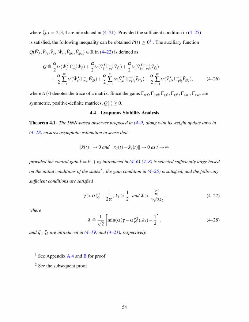
where ζi, i = 2,3,4 are introduced in (4–21). Provided the sufficient condition in (4–25)

is satisfied, the following inequality can be obtained P(t) ≥ 01 . The auxiliary functionQ(Wf ,Vf1 ,Vf2 ,Wgi,Vgi1 ,Vgi2) ∈ R in (4–22) is defined as

Q � α2

tr(W Tf Γ−1w f Wf )+

α2

tr(V Tf1Γ

−1v f1Vf1)+

α2

tr(V Tf2Γ

−1v f2Vf2)

+α2

m

∑i=1

tr(W Tgi Γ

−1wgi

Wgi)+α2

m

∑i=1

tr(V Tgi1Γ

−1vgi1Vgi1)+

α2

m

∑i=1

tr(V Tgi2Γ

−1vgi2Vgi2), (4–26)

where tr(·) denotes the trace of a matrix. Since the gains Γw f ,Γwgi,Γv f1 ,Γv f2 ,Γvgi1 ,Γvgi2 are

symmetric, positive-definite matrices, Q(·)≥ 0.4.4 Lyapunov Stability Analysis

Theorem 4.1. The DNN-based observer proposed in (4–9) along with its weight update laws in

(4–18) ensures asymptotic estimation in sense that

‖x(t)‖→ 0 and ‖x2(t)− x2(t)‖→ 0 as t → ∞

provided the control gain k = k1+k2 introduced in (4–6)-(4–8) is selected sufficiently large based

on the initial conditions of the states2 , the gain condition in (4–25) is satisfied, and the following

sufficient conditions are satisfied

γ > αζ 25 +1

2α, k1 >

1

2, and λ >

ζ 214√2k2

, (4–27)

where

λ � 1√2

[min(α(γ−αζ 25 ),k1)−

1

2

], (4–28)

and ζ1,ζ5 are introduced in (4–19) and (4–21), respectively.

1 See Appendix A.4 and B for proof

2 See the subsequent proof

54

Proof. Consider the Lyapunov candidate function VL(y) : D → R, which is a Lipschitz continu-

ous regular positive definite function defined as

VL � γ2

xT x+γ2

xTf x f +

γ2

ηT η +1

2rT r+P+Q, (4–29)

which satisfies the following inequalities:

U1(y)≤VL(y)≤U2(y). (4–30)

In (4–30),U1(y),U2(y) ∈ R are continuous positive definite functions defined as

U1(y)�min(γ2,1

2)‖y‖2 ,

U2(y)�max(γ2,1)‖y‖2 .

The generalized time derivative of (4–29) exists almost everywhere (a.e.), and VL(y) ∈a.e.·

V L(y)

(see Chapter 3 for further details) where

·VL = ∩

ξ∈∂VL(y)ξ T K

[ ·x

T ·x

T

f ηT rT 1

2P−

12 P1

2Q−

12 Q]T

, (4–31)

where ∂VL is the generalized gradient of VL(y) [96]. Since VL(y) is locally Lipschitz continuous

regular and smooth in y, (4–31) can be simplified as [97]

·VL = ∇V T

L K[ ·

xT ·

xT

f ηT rT 1

2P−

12 P1

2Q−

12 Q]T

=[γ xT γ xT

f γηT rT 2P12 2Q

12

]K [Ψ]T ,

where

Ψ �[ ·

xT ·

xT

f ηT rT 1

2P−

12 P1

2Q−

12 Q].

Using the calculus for K [·] from [98] (Theorem 1, Properties 2,5,7), and substituting the dy-namics from (4–5), (4–7)-(4–10), (4–13), (4–23), (4–24) and (4–26) and adding and subtracting

55

α(x+ x f )T N2 and using (4–16),

·VL(y) can be rewritten as

·VL ⊂ γ xT (r−α x−η)+ γ xT

f (η−α x f )+ γηT [−(k+α)r−αη + x− x f]

+ rT [N +N−β1K[sgn(x+ x f )

]− kr+ γ(k+α)η]

− γrT x− rT (N1−β1K[sgn(x+ x f )

])− (·x+

·x f )

T N2+√2ρ(‖z‖)‖z‖2

−α(x+ x f )T N2+α(x+ x f )

T {W Tf σ f +W T

f σ ′f [VTf1 x1+V T

f2 x2]

+m

∑i=1

W Tgi σgiui +

m

∑i=1

W Tgi σ

′gi[V

Tgi1 x1+V T

gi2 x2]ui

}

−αtr(W Tf Γ−1w f

·W f )−αtr(V T

f1Γ−1v f1

·V f1)−αtr(V T

f2Γ−1v f2

·V f2) (4–32)

−αm

∑i=1

tr(W Tgi Γ

−1wg

·W gi)−α

m

∑i=1

tr(V Tgi1Γ

−1vgi1

·V gi1)−α

m

∑i=1

tr(V Tgi2Γ

−1vgi2

·V gi2).

Using the fact that K[sgn(x+ x f )] = SGN(x+ x f ) (see Chapter 3 for further details), the set in

(4–32) can reduce to the scalar inequality. Substituting the weight update laws in (4–18) and

canceling common terms, the above expression can be upper bounded as

·VL

a.e.≤ −αγ xT x−αγ xTf x f −αγηT η− krT r

+α(x+ x f )T N2+ rT N +

√2ρ(‖z‖)‖z‖2 . (4–33)

Using (4–19), (4–21), the fact that

αζ5∥∥x+ x f

∥∥‖z‖ ≤ α2ζ 25 ‖x‖2+α2ζ 25∥∥x f∥∥2+ 1

2‖z‖2 ,

substituting k = k1+ k2, and completing the squares, the expression in (4–33) can be further

bounded as

·VL

a.e.≤ −α(γ−αζ 25 )‖x‖2−α(γ−αζ 25 )∥∥x f∥∥2−αγ ‖η‖2

− k1 ‖r‖2+(1

2+

ζ 214k2

+√2ρ(‖z‖)

)‖z‖2 .

56

Provided the sufficient conditions in (4–27) are satisfied, the above expression can be rewritten as

·V

a.e.≤ −√2(λ − ζ 21

4√2k2

−ρ(‖z‖))‖z‖2 a.e.≤ −U(y) ∀y ∈D , (4–34)

where λ is defined in (4–28) andU(y) = c‖z‖2, for some positive constant c, is a continuous

positive semi-definite function which is defined on the domain

D �{

y(t) ∈ R4n+2|‖y(t)‖ ≤ ρ−1(λ − ζ 214√2k2

)

}.

The size of the domain D can be increased by increasing the gains k and α . The inequalities

in (4–30) and (4–34) show that V (y) ∈L∞ in the domain D ; hence, x(t), x f (t),η(t),r(t),P(t)

and Q(t) ∈ L∞ in D ; (4–5)-(4–10) are used to show that·x(t),

·x f (t), η(t) ∈ L∞ in D . Since

x1(t),x2(t) ∈L∞ by Assumption 4.1, x1(t), x2(t) ∈L∞ in D using (4–4). Since x(t), x f (t),η(t) ∈L∞ in D , using (4–12), v(t) ∈ L∞ in D . SinceWf ,Wgi,σ f (·),σgi(·),ε f (·),εgi(·) ∈ L∞, i =

1...m, by Assumptions 4.4-4.6, the control input u(t) and the disturbance d(t) are bounded by

Assumptions 4.2-4.3, and Wf (t),Wgi(t) ∈ L∞, i = 1...m, by the use of the pro j(·) algorithm,from (4–11), r(t) ∈L∞ in D ; then z(t) ∈L∞ in D , by using (4–20). Hence,U(y) is uniformly

continuous in D . Let S⊂D denote a set defined as

S �{

y(t) ∈D |U2(y(t))< ε1(ρ−1(λ − ζ 214√2k2

))2}. (4–35)

The region of attraction in (4–35) can be made arbitrarily large to include any initial condition by

increasing the control gains k and α (i.e., a semi-global type of stability result), and hence

c‖z‖2→ 0 as t → ∞ ∀y(0) ∈S .

Based on the definition of z(t) the following result can be proven

‖x(t)‖ ,‖η(t)‖ ,‖r(t)‖→ 0 as t → ∞ ∀y(0) ∈S .

57

From (4–5), it can be further shown that

∥∥∥∥ ·x(t)∥∥∥∥→ 0 as t → ∞ ∀y(0) ∈S .

4.5 Extension for High-order Uncertain Nonlinear Systems

The proposed method can be extended for a Nth order uncertain nonlinear system as

x1 = x2,

...

xN−1 = xN , (4–36)

xN = f (x)+G(x)u+d,

y = x1,

where x(t) =[xT1 (t) xT

2 (t) . . .xTN(t)

]T∈ RNn is the system state, the system output y(t) ∈ R

n is

measurable up to N− 1th derivatives, i.e. xi(t), i = 1,2..,N− 1 are measurable, and xN(t) is

unmeasurable, and the unknown functions f (x),G(x), the control input u(t) and the disturbance

d(t) are introduced in (4–1).

Given the system in (4–36), the observer in (4–9) can be extended as

˙x1 = x2,

...

˙xN−1 = xN , (4–37)

˙xN = W Tf σ f +

m

∑i=1

W Tgi σgiui + v,

where x(t)=[xT1 (t) xT

2 (t) . . . xTN(t)

]T∈ RNn is the state of the DNN observer, Wf (t), Vf j(t), Wgi(t),

Vgi j(t), i = 1...m, j = 1 . . .N, and σ f (t), σgi(t) are introduced in (4–9) and the robust control term

58

v(t) ∈ Rn is modified as

v �− [γK +2αN−1]η +(γ−α2N−1)xN−1+β1sgn(xN−1+ x f ). (4–38)

In (4–38), K,γ,αN−1,β1 ∈ R are positive constant gains, and x f (t),η(t) ∈ Rn are outputs of the

modified dynamic filter

η = p−KxN−1,

p =−(K +αN−1)p− x f +(K2+1)xN−1, (4–39)

·x f = p−αN−1x f −KxN−1,

p(0) = KxN−1(0), x f (0) = 0.

The estimation error x1(t) ∈ Rn and the following filtered estimation errors xi(t) ∈ R

n, i =

1, . . . ,N−1 are defined as

x1 � x1− x1,

x2 � ˙x1+α1x1,

xi � ˙xi−1+αi−1xi−1+ xi−2, i = 3, . . . ,N−1,

r � ˙xN−1+αN−1xN−1+η , (4–40)

where αi ∈ R, i = 1,2, . . . ,N − 2, are positive constant control gains. Note that the signalsxi(t), i = 1, . . . ,N− 1 are measurable, whereas, the filtered estimation error r(t) in (4–40) is

not measurable, since it depends on xN(t). The weight update laws for the DNN in (4–37) are

developed as

·W f = pro j[Γw f σ f (xN−1+ x f )

T ],

·V f j = pro j[Γv f j x j(xN−1+ x f )

TW Tf σ ′f ],

·W gi = pro j[Γwgiσgiui(xN−1+ x f )

T ],

·V gi j = pro j[Γvgi j x jui(xN−1+ x f )

TW Tgi σ

′gi],

59

Figure 4-1. The experimental testbed consists of a two-link robot. The links are mounted on two

NSK direct-drive switched reluctance motors.

where i = 1...m, j = 1 . . .N, Γw f , Γwgi, Γv f j , Γvgi j , σ ′f (t), σ ′gi(t) are introduced in (4–18).

A similar stability analysis can be used to prove that

‖xi(t)‖ ,‖η(t)‖ ,‖r(t)‖→ 0 as t → ∞, i = 1,2, . . . ,N−1.

From (4–40), it can be further shown that

∥∥∥x(N)1 (t)− x(N)

1 (t)∥∥∥→ 0 as t → ∞.

4.6 Experiment and Simulation Results

Experiments and simulations on a two-link robot manipulator (Fig. 4-1) are performed to

compare the proposed method with several other estimation methods. The testbed is composed

of a two-link direct drive revolute robot consisting of two aluminum links. The motor encoders

provide position measurements with a resolution of 614400 pulses/revolution. Two aluminum

links are mounted on a 240 Nm (first link) and a 20 Nm (second link) switched reluctance

motor. Data acquisition and control implementation were performed in real-time using QNX at a

60

frequency of 1.0 kHz. The two-link revolute robot is modeled with the following dynamics:

M(x)x+Vm(x, x)x+Fdx+Fs(x) = u(t), (4–41)

where x =

[x1 x2

]T

are the angular positions (rad) and x =

[x1 x2

]T

are the angular

velocities (rad/s) of the two links respectively. In (4–41),M(x) is the inertia matrix and Vm(x, x)

is the centripetal-Coriolis matrix, defined as

M �

⎡⎢⎣ p1+2p3c2 p2+ p3c2

p2+ p3c2 p2

⎤⎥⎦ ,

Vm �

⎡⎢⎣ −p3s2x2 −p3s2 (x1+ x2)

p3s2x1 0

⎤⎥⎦ . (4–42)

In (4–41) and (4–42), parameters for simulation are chosen as the best-guess of the testbed model

as p1 = 3.473 kg ·m2, p2 = 0.196 kg ·m2, p3 = 0.242 kg ·m2, c2 = cos(x2), s2 = sin(x2).

Fd = diag{5.3,1.1}Nm · sec and Fs(x) = diag{8.45tanh(x1),2.35tanh(x2)}Nm are the models

for dynamic and static friction, respectively. The system in (4–41) can be rewritten as

x = f (x, x)+G(x, x)u+d,

where d(t) ∈ R2 is the additive exogenous disturbance and f (x, x) ∈ R

2, and G(x, x) ∈ R2×2 are

defined as

f (x, x) = M−1 (−Vm−Fd) x−Fs, G(x, x) = M−1.

The control input is chosen as a PD controller to track a desired trajectory xd(t) =

[0.5sin(2t) 0.5cos(2t)]T , as u(t) = 20(x(t)− xd(t)) + 10(x(t)− xd(t)), where the angular

velocity x(t) used only in the control law is determined numerically by a standard backwards

difference algorithm. The objective is to design an observer ˙x(t) to asymptotically estimate the

angular velocities x(t) using only the measurements of angular positions x(t). The control gains

for the experiment are chosen as k = 7, α = 7, γ = 8, β1 = 6, and Γw f = Γwg1 = Γwg2 = 3I8×8,

61

5 5.1 5.2 5.3 5.4 5.5 5.6 5.7 5.8 5.9 6−50

0

50

100

˙ x(t)(deg/s)

(a) Velocity Estimation at Steady State (Xian observer)

5 5.1 5.2 5.3 5.4 5.5 5.6 5.7 5.8 5.9 6−50

0

50

100

˙ x(t)(deg/s)

(b) Velocity Estimation at Steady State (High gain observer)

5 5.1 5.2 5.3 5.4 5.5 5.6 5.7 5.8 5.9 6−50

0

50

100

˙ x(t)(deg/s)

(c) Velocity Estimation at Steady State (Proposed)

5 5.1 5.2 5.3 5.4 5.5 5.6 5.7 5.8 5.9 6−50

0

50

100

time (s)

˙ x(t)(deg/s)

(d) Velocity Estimation at Steady State (Central Difference)

Figure 4-2. Velocity estimate ˙x(t) using (a) [1], (b) [2], (c) the proposed method, and (d) thecenter difference method on a two-link experiment testbed.

Γv f = Γvg1 = Γvg2 = 3I2×2, where In×n denotes an identity matrix of appropriate dimensions.

The NNs are designed to have seven hidden layer neurons and the NN weights are initialized as

uniformly distributed random numbers in the interval [−1,1]. The initial conditions of the systemand the identifier are chosen as x(t) = [0 0]T , x(t) = [0 0]T and x(t) = ˙x(t) = [0 0]T , respectively.

A global asymptotic velocity observer for uncertain nonlinear systems was developed by

Xian et al. [1] as

˙x = p+K0x, p = K1sgn(x)+K2x,

and a high gain (HG) observer that is asymptotic as the gain goes to infinity was developed in [2]

˙x = zh +αh1

εh1x, zh =

αh2

εh2x.

Both these designs are based on a purely robust feedback strategy. A contribution of this work is

the addition of a feed-forward adaptive component to compensate for the uncertain dynamics. To

gauge the benefit of this approach, the proposed observer is compared with the observers in [1]

and [2]. Control gains for the observer in [1] are chosen as K0 = 10, K1 = 6, and K2 = 10, and

control gains for the HG observer are chosen as α1 = 0.6, α2 = 25, ε1 = 0.01, and ε2 = 0.015.

62

5 5.1 5.2 5.3 5.4 5.5 5.6 5.7 5.8 5.9 6−50

0

50

100

˙ x(t)(deg/s)

(a) Velocity Estimation at Steady State (Xian observer)

5 5.1 5.2 5.3 5.4 5.5 5.6 5.7 5.8 5.9 6−50

0

50

100˙ x(t)(deg/s)

(b) Velocity Estimation at Steady State (High gain observer)

5 5.1 5.2 5.3 5.4 5.5 5.6 5.7 5.8 5.9 6−50

0

50

100

˙ x(t)(deg/s)

(c) Velocity Estimation at Steady State (Proposed)

5 5.1 5.2 5.3 5.4 5.5 5.6 5.7 5.8 5.9 6−50

0

50

100

time (s)

˙ x(t)(deg/s)

(d) Velocity Estimation at Steady State (Central Difference)

Figure 4-3. The steady-state velocity estimate ˙x(t) using (a) [1], (b) [2], (c) the proposed method,and (d) the center difference method on a two-link experiment testbed.

0 10 20 30 40 50 60 700

0.02

0.04

Magnitude

(a) Frequency Analysis (Xian observer)

0 10 20 30 40 50 60 700

0.02

0.04

Magnitude

(b) Frequency Analysis (High gain observer)

0 10 20 30 40 50 60 700

0.02

0.04

Magnitude

(c) Frequency Analysis (Proposed)

0 10 20 30 40 50 60 700

0.02

0.04

frequency (Hz)

Magnitude

(d) Frequency Analysis (Central difference)

Figure 4-4. Frequency analysis of velocity estimation ˙x(t) using (a) [1], (b) [2], (c) the proposedmethod, and (d) the center difference method on a two-link experiment testbed.

63

To make the comparison feasible, the gains of all observers are tuned to get the steady state root

mean squares (RMS) of position estimation errors to be approximately equal 0.17 for a settling

time of 1 second. The experiment results for the velocity estimators in [1], [2], and the proposed

method are compared with the central difference algorithm. The results are shown in Figs. 4-2

and 4-3. It is observed that the velocity estimates of the proposed observer and observer in [2]

look similar, but the transient response of the proposed method is improved over the observer

in [2]; moreover, both methods lower frequency content than the observer in [1] and the central

difference method. To illustrate the lower frequency response of the proposed method compared

to [1] and the central difference method, the frequency analysis plots of the experiment results

are shown in Fig. 4-4. Fig. 4-4 illustrates that the velocity estimation using [1] and central

difference methods include higher frequency signals than the proposed method or the approach

in [2].

Given the lack of velocity sensors in the two-link experiment testbed to verify the velocity

estimates, a simulation was performed using the dynamics in (4–41). To examine the effect of

noise, white Gaussian noise with SNR 60 dB is added to the position measurements. Fig. 4-5

shows the simulation results for the steady-state velocity estimation errors and the respective

frequency analysis for the velocity estimate of the observer in [1], the observer in [2], the

developed method, and the central difference method. Table 4-1 gives a comparison of the

transient and steady state RMS velocity estimation errors for these different methods. Results

of the standard numerical central differentiation algorithm are significantly worse than the other

methods in the presence of noise as seen from Fig. 4-5 and Table 4-1. Although, simulation

results for [2] and the developed method are comparable, differences exist in the structure of

the observers and proof of convergence of the estimates. The observer in [2] is a purely robust

feedback technique and the estimation result is proven to be asymptotic as the gains tend to

infinity. On the other hand, the proposed method is a robust adaptive observer with a DNN

structure to learn the system uncertainties, combining a dynamic filter and a robust sliding mode

structure, thus guaranteeing asymptotic convergence with finite gains. Further, the observer in [1]

64

1 1.5 2 2.5 3−0.2

0

0.2

˙ x(t)(rad/s)

(a) Estimation Error at Steady−state (Xian observer)

1 1.5 2 2.5 3−0.2

0

0.2

˙ x(t)(rad/s)

(b) Estimation Error at Steady−state (High gain observer)

1 1.5 2 2.5 3−0.2

0

0.2

˙ x(t)(rad/s)

(c) Estimation Error at Steady−state (Proposed)

1 1.5 2 2.5 3−20

0

20

Time (s)

˙ x(t)(rad/s)

(d) Estimation Error at Steady−state (Central Difference)

0 20 40 60 80 1000

0.005

0.01

0.015

Magnitude

(e) Frequency Analysis (Xian observer)

0 20 40 60 80 1000

0.005

0.01

0.015

Magnitude

(f) Frequency Analysis (High gain observer)

0 20 40 60 80 1000

0.005

0.01

0.015

Magnitude

(g) Frequency Analysis (Proposed)

0 20 40 60 80 1000

1

2

3

frequency (Hz)

Magnitude

(h) Frequency Analysis (Central difference)

Figure 4-5. The steady-state velocity estimation error ˙x(t) using (a) [1], (b) [2], (c) the proposedmethod, and (d) the center difference method on simulations, in presence of sensor

noise (SNR 60dB). The right figures (e)-(h) indicate the respective frequency analysis

of velocity estimation ˙x(t).

is also a purely robust feedback method, where all uncertainties are damped out by a sliding

mode term resulting in higher frequency velocity estimates than the developed observer, as seen

from both experiment and simulation results.

4.7 Conclusion

A novel design of an adaptive observer using DNNs for uncertain nonlinear systems is

proposed. The DNN works in conjunction with a dynamic filter without any off-line training

Table 4-1. Transient (t = 0−1 sec) and steady state (t = 1−10 sec) velocity estimation errors˙x(t) for different velocity estimation methods in presence of noise 50dB.

Central difference Method in [1] Method in [2] Proposed

Transient RMS Error 66.2682 0.1780 0.1040 0.1309

Steady State RMS Error 8.1608 0.0565 0.0538 0.0504

65

phase. A sliding feedback term is added to the DNN structure to account for reconstruction

errors and external disturbances. The observation states are proven to asymptotically converge

to the system states and a similar observer structure is extended to high-order uncertain systems.

Simulations and experiments show the improvement of the proposed method in comparison to

several other estimation methods.

66

CHAPTER 5

GLOBAL OUTPUT FEEDBACK TRACKING CONTROL FOR UNCERTAIN

SECOND-ODER NONLINEAR SYSTEMS

A DNN observer-based OFB controller for uncertain nonlinear systems with bounded

disturbances is developed. A two-fold objective, asymptotic estimation of unmeasurable states

and asymptotic tracking control, is set up. The asymptotic estimation of the unmeasurable state

is achieved by exploiting the DNN-based observer in Chapter 4, wherein the dynamic filter

and the weight update laws are modified for the new objective. A robust controller includes a

NN feedforward term, along with the estimated state feedback and sliding mode terms through

the Lyapunov-based stability analysis to yield an asymptotic tracking result. The developed

method yields the first OFB technique simultaneously achieving asymptotic tracking and

asymptotic estimation of unmeasurable states for the class of uncertain nonlinear systems with

bounded disturbances. Experiments on a two-link robot manipulator are used to investigate the

performance of the proposed control approach.


Consider a control-affine second order Euler-Lagrange like nonlinear system of the form

x = f (x, x)+G(x)u+d, (5–1)

where x(t) ∈ Rn is the measurable output with a finite initial condition x(0) = x0, u(t) ∈ R

n

is the control input, f (x, x) ∈ Rn,G(x) ∈ R

n×n are continuous functions, and d(t) ∈ Rn is an

exogenous disturbance. The following assumptions about the system in (5–1) will be utilized in

the subsequent development.

Assumption 5.1. The time derivatives of the system output x(t), x(t) are unmeasurable.

Assumption 5.2. The unknown function f (x, x) is C1, and the function G(x) is known, invertible

and the matrix inverse G−1(x) is bounded.

Assumption 5.3. The disturbance d(t) is differentiable, and d(t), d(t) ∈L∞.

67

Based on the universal approximation property of MLNNs, the unknown function f (x, x) in

(5–1) can be replaced by a MLNN, and the system can be represented as

x =W T σ(V T1 x+V T

2 x)+ ε +Gu+d, (5–2)

whereW ∈ RN+1×n, V1,V2 ∈ R

n×N are unknown ideal weight matrices of the MLNN having N

hidden layer neurons, σ(t) � σ(V T1 x(t)+V T

2 x(t)) ∈ RN+1 is the activation function (sigmoid,

hyperbolic tangent etc.), and ε(x, x) ∈ Rn is a function reconstruction error. The following

assumptions will be used in the DNN-based observer and controller development and stability

analysis.

Assumption 5.4. The ideal NN weights are bounded by known positive constants [46], i.e.

‖W‖ ≤ W , ‖V1‖ ≤ V1, ‖V2‖ ≤ V2.

Assumption 5.5. The activation function σ(·) and its partial derivatives σ ′(·), σ ′′(·) are

bounded [46]. This assumption is satisfied for typical activation functions (e.g., sigmoid,

hyperbolic tangent).

Assumption 5.6. The function reconstruction error ε(x, x), and its first time derivative are

bounded [46], as ‖ε(x, x)‖ ≤ ε1, ‖ε(x, x, x)‖ ≤ ε2, where ε1, ε2 are known positive constants.

5.2 Estimation and Control Objectives

The contribution in this chapter is the development of a robust DNN-based observer

such that the estimated states asymptotically converge to the states of the system (5–1), and a

discontinuous controller enables the system state to asymptotically track a desired time-varying

trajectory xd(t) ∈ Rn, despite uncertainties and disturbances in the system. To quantify these

objectives, an estimation error x(t) ∈ Rn and a tracking error e(t) ∈ R

n are defined as

x � x− x, (5–3)

e � x− xd, (5–4)

where x(t) ∈ Rn is the state of the DNN observer which is introduced in the subsequent develop-

ment. The desired trajectory xd(t) and its derivatives x(i)d (t) (i = 1,2), are assumed to exist and be

68

bounded. To compensate for the lack of direct measurements of x(t), the filtered estimation error

res(t) ∈ Rn and the filtered tracking error rtr(t) ∈ R

n are defined as

res �·x+α x+η , (5–5)

rtr �·e+αe+η , (5–6)

where α ∈ R is a positive constant gain, and η(t) ∈ Rn is an output of the dynamic filter

η = p− (k+α)x,

p =−(k+2α)p−ν +((k+α)2+1)x+ e,

ν = p−αν− (k+α)x, (5–7)

p(0) = (k+α)x(0), ν(0) = 0,

where ν(t) ∈ Rn is another output of the filter, p(t) ∈ R

n is used as an internal filter variable,

and k ∈ R is a positive constant control gain. The filtered estimation error res(t) and the filtered

tracking error rtr(t) are not measurable since the expressions in (5–5) and (5–6) depend on x(t).

5.3 DNN-based Robust Observer

The MLDNN architecture is developed to observe the system in (5–1)

··x = W T σ +Gu− (k+3α)η +β1sgn(x+ν), (5–8)

where

[x(t)T

·x(t)T

]T

∈ R2n are the states of the DNN observer, W (t) ∈ R

N+1×n, V1(t),V2(t) ∈

Rn×N are the weight estimates, σ(t) � σ(V1(t)T x(t)+ V2(t)T

·x(t)) ∈ R

N+1 and β1 ∈ R is a

positive constant control gain.

69



·W = Γw pro j[σd(x+ e+2ν)T ],

·V 1 = Γv1pro j[xd(x+ e+2ν)TW T σ ′d], (5–9)

·V 2 = Γv2pro j[xd(x+ e+2ν)TW T σ ′d],

where Γw ∈ R(N+1)×(N+1), Γv1,Γv2 ∈ R

n×n, are constant symmetric positive-definite adaptation

gains, the terms σd(t), σ ′d(t) are defined as σd(t) � σ(V1(t)T xd(t) + V2(t)T xd(t)), σ ′d(t) �

dσ(ς)/dς |ς=V T1 xd+V T

2 xd, and pro j(·) is a smooth projection operator [88], [89] used to guarantee

that the weight estimates W (t),V1(t),V2(t) remain bounded.

To facilitate the subsequent analysis, (5–5) and (5–7) can be used to express the time

derivative of η(t) as

η =−(k+α)res−αη + x+ e−ν . (5–10)

The closed-loop dynamics of the filtered estimation error in (5–5) can be determined by using

(5–2), (5–3), (5–5), (5–8) and (5–10) as

res =W T σ −W T σ + ε +d +(k+3α)η−β1sgn(x+ν)

+α(res−α x−η)− (k+α)res−αη + x+ e−ν . (5–11)

Adding and subtractingW T σd +W T σd +W T σd where σd(t) � σ(V T1 xd(t)+V T

2 xd(t)), the

expression in (5–11) can be rewritten as

res = N1+N− kres−β1sgn(x+ν)+(k+α)η− x, (5–12)

where the auxiliary function N1(e, x,ν ,res,rtr,W ,V1,V2, t) ∈ Rn is defined as

N1 �W T (σ −σd)−W T (σ − σd)− (α2−2)x−ν + e, (5–13)

70

and N(xd,·xd,W ,V1,V2, t) ∈ R

n is segregated into two parts as

N � ND +NB. (5–14)

In (5–14), ND(t), NB(W ,V1,V2, t) ∈ Rn are defined as

ND � ε +d, (5–15)

and

NB � NB1+NB2 . (5–16)

In (5–16), NB1(W ,V1,V2, t),NB2(W ,V1,V2, t) ∈ Rn are defined as

NB1 �W T O(V T1 xd +V T

2 xd)2+W T σ ′d(V

T1 xd +V T

2 xd),

NB2 � W T σd +W T σ ′d(VT1 xd +V T

2 xd), (5–17)

where W (t)�W −W (t) ∈RN+1×n, V1(t)�V1−V1(t) ∈R

n×N , V2(t)�V2−V2(t) ∈Rn×N are the

estimate mismatches for the ideal NN weights, and O(V T1 xd + V T

2 xd)2 ∈ R

N+1 is the higher order

term in the Taylor series of the vector functions σd(·) in the neighborhood of V T1 xd +V T

2 xd as

σd = σd + σ ′d(VT1 xd +V T

2 xd)+O(V T1 xd +V T

2 xd)2. (5–18)

Motivation for segregating the terms in (5–12), (5–14) and (5–16) is derived from the fact that

different terms have different bounds. The term N1(·) includes all terms which can be upperbounded by states, whereas N(·) includes all terms which can be upper bounded by constants.The difference between the terms ND(·) and NB(·) in (5–14) which both can be upper-bounded byconstants is that the first time derivative of ND(·) is further upper-bounded by a constant, whereasthe term NB(·) is state dependent. The term NB(·) is further segregated as (5–16) to aid in theweight update law design for the DNN in (5–9). In subsequent stability analysis, the term NB1(·)is cancelled by the error feedback and the sliding mode term, while the term NB2(·) is partiallycompensated for by the weight update laws and partially cancelled by the error feedback and the

sliding mode term.

71

Using (5–3)-(5–6), Assumptions 5.4-5.5, the pro j(·) algorithm in (5–9) and the Mean ValueTheorem, the auxiliary function N1(t) in (5–13) can be upper-bounded as

∥∥N1∥∥≤ ζ1 ‖z‖ , (5–19)

where ζ1 ∈ R is a computable positive constant, and z(x,e,res,rtr,ν ,η) ∈ R6n is defined as

z � [xT eT rTes rT

tr νT ηT ]T . (5–20)

Based on Assumptions 5.3-5.6, the Taylor series expansion in (5–18), and the weight update laws

in (5–9), the following bounds can be developed

‖ND‖ ≤ ζ2, ‖NB1‖ ≤ ζ3, ‖NB2‖ ≤ ζ4, (5–21)∥∥ND∥∥≤ ζ5,

∥∥NB∥∥≤ ζ6+ζ7 ‖z‖ ,

where ζi ∈ R, i = 2,3, ...,7, are computable positive constants.

5.4 Robust Adaptive Tracking Controller

The control objective is to force the system state to asymptotically track the desired

trajectory xd(t), despite the uncertainties and disturbances in the system. Quantitatively, this

objective is to regulate the filtered tracking controller rtr(t) to zero. Using (5–2), (5–4), (5–6)

and (5–10), the open-loop dynamics of the derivative of the filtered tracking error in (5–6) is

expressed as

rtr =W T σ +G(x)u+ ε +d− xd +α(rtr−αe−η)

− (k+α)res−αη + x+ e−ν . (5–22)

The control input u(t) is now designed as a composition of the DNN term, the estimated states

x(t),·x(t), and the sliding mode term as

u(t) = G−1[xd−W T σd− (k+α)(·e+α e)−β2sgn(e+ν)], (5–23)

72

where β2 ∈ R is a positive constant control gain and the tracking error estimate e(t) ∈ Rn is

defined as

e � x− xd.

Based on the fact that the estimated states are measurable, the tracking error estimate e(t) and its

derivative·e(t) are measurable; moreover, the filtered tracking error rtr(t) is related to the filtered

estimation error res(t) via the tracking error estimate e(t) as

rtr = res +·e+α e. (5–24)

Hence, adding and subtractingW T σd +W T σd and using (5–22)-(5–24), the closed-loop error

system becomes

rtr = N2+N− krtr−β2sgn(e+ν)− e, (5–25)

where the auxiliary function N2(e, x,η ,ν ,rtr, t) ∈ Rn is defined as

N2 �W T (σ −σd)− (α2−2)e−ν + x−2αη , (5–26)

and the function N(·) is introduced in (5–14). Similarly, using (5–4), (5–6), Assumptions 5.4-5.5,the pro j(·) algorithm in (5–9), and the Mean Value Theorem [74], the auxiliary function N2(·) in(5–26) can be upper-bounded as ∥∥N2

∥∥≤ ζ8 ‖z‖ , (5–27)

where ζ8 ∈ R is a computable positive constant.

To facilitate the subsequent stability analysis, let y(z,P,Q) ∈ R6n+2 be defined as

y � [zT√

P√

Q]T . (5–28)

73

In (5–28), the auxiliary function P(res,rtr, x,e,ν ,·x, e, ν , t) ∈ R is the Filippov solution to the

differential equation

P � L, (5–29)

P0 � P(x(0),e(0),ν(0),0)

= β1n

∑j=1

∣∣x j(0)+ν j(0)∣∣+β2

n

∑j=1

∣∣ej(0)+ν j(0)∣∣− (x(0)+ e(0)+2ν(0))T N (0) ,

where the subscript j = 1,2, ..,n denotes the jth element of x(0), e(0) or ν(0), and the auxiliary

function L(res,rtr, x,e,ν ,·x, e, ν , t) ∈ R is defined as

L �−rTes(ND +NB1−β1sgn(x+ν))− rT

tr(ND +NB1−β2sgn(e+ν))

− (·x+ e+2ν)T NB2+β3 ‖z‖2 , (5–30)

where β1, β2 are introduced in (5–8) and (5–23), and β3 ∈ R is a positive constant. The control

gains βi, i = 1,2,3 are chosen according to the sufficient conditions

β1,β2 >max(ζ2+ζ3+ζ4,ζ2+ζ3+ζ5α

+ζ6α), β3 > 2ζ7, (5–31)

where ζi, i = 1,2, ...,7 are introduced in (5–19) and (5–21). Provided the sufficient conditions in

(5–31) are satisfied, the following inequality can be obtained P(·) ≥ 01 . The auxiliary functionQ(W ,V1,V2) ∈ R in (5–28) is defined as

Q(t)� α2

tr(W T Γ−1w W )+α2

tr(V T1 Γ−1v1 V1)+

α2

tr(V T2 Γ−1v2 V2), (5–32)

where tr(·) denotes the trace of a matrix. Since the gains Γw,Γv1,Γv2 are symmetric, positive-

definite matrices, Q(·)≥ 0.

1 See Appendix B for proof

74

5.5 Lyapunov Stability Analysis for DNN-based Observation and Control

Theorem 5.1. The DNN-based observer and controller proposed in (5–8) and (5–23), respec-

tively, along with the weight update laws in (5–9) ensure asymptotic estimation and tracking in

sense that

‖x(t)‖→ 0 and∥∥∥∥ ·x(t)

∥∥∥∥→ 0 as t → ∞,

‖e(t)‖→ 0 and ‖e(t)‖→ 0 as t → ∞,

provided the gain conditions in (5–31) are satisfied, and the control gains α and k = k1+ k2

introduced in (5–5)-(5–7) are selected as

λ �min(α,k1)>ζ 21 +ζ 284k2

+β3, (5–33)

whereζ1,ζ8,β3 are introduced in (5–19), (5–27), and (5–30), respectively.

Proof. Consider the Lyapunov candidate function VL(y, t) : D×(0,∞)→ R, which is a Lipschitz

continuous regular positive definite function defined as

VL � 1

2xT x+

1

2eT e+

1

2νT ν +

1

2ηT η +

1

2rT

esres +1

2rTtrrtr +P+Q, (5–34)


U1(y)≤VL(y, t)≤U2(y). (5–35)

In (5–35),U1(y),U2(y) ∈ R are continuous positive definite functions defined as

U1(y)�1

2‖y‖2 , U2(y)� ‖y‖2 .

The generalized time derivative of (5–34) exists almost everywhere (a.e.), and VL(y) ∈a.e.·

V L(y)

(see Chapter 3 for further details) where

·VL = ∩

ξ∈∂VL(y)ξ T K

[ ·x

TeT νT ηT rT

es rTtr1

2P−

12 P1

2Q−

12 Q]T

, (5–36)

75

where ∂VL is the generalized gradient of VL(y) [96]. Since VL(y) is a locally Lipschitz continuous

regular function that is smooth in y, (5–36) can be simplified as [97]

·VL = ∇V T K

[ ·x

TeT νT ηT rT

es rTtr1

2P−

12 P1

2Q−

12 Q]T

=[xT eT νT ηT rT

es rTtr 2P

12 2Q

12

]K [Ψ]T ,

where

Ψ �[ ·

xT

eT νT ηT rTes rT

tr1

2P−

12 P1

2Q−

12 Q].

Using the calculus for K [·] from [98] (Theorem 1, Properties 2,5,7), and substituting thedynamics from (5–5)-(5–7), (5–10), (5–12), (5–25), (5–29), (5–30) and (5–32),

·V L(y) can be

rewritten as

·VL ⊂ xT (res−α x−η)+ eT (rtr−αe−η)+ηT [−(k+α)res−αη + x+ e−ν ]

+νT (η−αν)+ rTes{

N1+N− kres−β1K[sgn(x+ν)]+(k+α)η− x}

+ rTtr{

N2+N− krtr−β2K[sgn(e+ν)]− e}− rT

es {ND +NB1−β1K[sgn(x+ν)]}

− rTtr {ND +NB1−β2K[sgn(e+ν)]}+β3 ‖z‖2− (

·x+ e+2ν)T NB2

−αtr(W T Γ−1w

·W )−αtr(V T

1 Γ−1v1

·V 1)−αtr(V T

2 Γ−1v2

·V 2). (5–37)

Using the fact that K[sgn(e+ν)] = SGN(e+ν) and K[sgn(x+ν)] = SGN(x+ν) (see Chapter

3 for further details), the set in (5–37) can reduce to the scalar inequality. Substituting the weight

update laws in (5–9) and canceling common terms, the above expression can be upper bounded

as

·VL

a.e.≤ −α xT x−αeT e−ανT ν−αηT η− krTesres− krT

trrtr + rTesN1+ rT

trN2+β3 ‖z‖2 . (5–38)

76

Using (5–19) and (5–27), substituting k = k1+ k2, and completing the squares, the expression in

(5–38) can be further bounded as

·VL

a.e.≤ −α ‖x‖2−α ‖e‖2−α ‖ν‖2−α ‖η‖2− k1 ‖res‖2− k1 ‖rtr‖2+(

ζ 21 +ζ 284k2

+β3)‖z‖2

a.e.≤ −(λ − ζ 21 +ζ 284k2

−β3)‖z‖2a.e.≤ −U(y), (5–39)

whereU(y) = c‖z‖2, for some positive constant c, is a continuous positive semi-definite function,

and λ is defined in (5–33). The inequalities in (5–35) and (5–39) show that VL(y) ∈L∞; hence,

x(t), e(t),ν(t), η(t), res(t), rtr(t), P(t) and Q(t) ∈L∞. Using (5–5) and (5–6), it can be shown

that·x(t), e(t) ∈ L∞. Based on the assumption that xd(t), xd(t) ∈ L∞, and e(t), e(t) ∈ L∞,

x(t), x(t) ∈L∞ by (5–4); moreover, using (5–3) and x(t),·x(t) ∈L∞, x(t),

·x(t) ∈L∞. Based on

Assumptions 5.2 and 5.5, the projection algorithm in (5–9), the boundedness of the sgn(·) andσ(·) functions, and xd(t), xd(t), x(t),

·x(t) ∈L∞, the control input u(t) is bounded from (5–23).

Similarly, ν(t), η(t), res(t), rtr(t) ∈L∞ by using (5–7), (5–10), (5–11), (5–25); hence z(t) ∈L∞,

using (5–20); hence,U(y) is uniformly continuous. It can be concluded that

c‖z‖2→ 0 as t → ∞,

and using the definition of z(t) in (5–20), the following result can be shown

‖x‖ ,‖e‖→ 0 as t → ∞,

‖res‖ ,‖rtr‖ ,‖ν‖ ,‖η‖→ 0 as t → ∞.

Using (5–5) and (5–6), and standard linear analysis, it can be further shown that

∥∥∥∥ ·x∥∥∥∥ ,‖e‖→ 0 as t → ∞.

77

5.6 Experiment Results

The performance of the proposed OFB control method is tested on a two-link robot

manipulator depicted in Fig. 4-1, where the dynamics given by (4–41). The desired trajectory for

each link of the manipulator is given as (in degrees)

x1d = 30sin(1.5t)(1− exp(−0.01t3)),

x2d = 30sin(2.0t)(1− exp(−0.05t3)).

The control gains are chosen as k = diag(25, 90), α = diag(22, 30), β1 = 0.2, β2 = 0.2

and, Γw = 0.2I8×8, Γv1 = Γv2 = 0.2I2×2, where In×n denotes an identity matrix of appropriate

dimensions. The NNs was implemented with 7 hidden layer neurons and the NN weights

are initialized as uniformly distributed random numbers in the interval [0.1,0.3]. The initial

conditions of the system and the observer were selected as x(t) = [0 0]T , x(t) = [0 0]T , and

x(t) = ˙x(t) = [0 0]T , respectively.

The performance of the proposed OFB controller is compared with two controllers: a

classical PID controller, and the discontinuous OFB controller in [1]. A standard backwards

difference algorithm is used to numerically determine velocity from the encoder readings to

implement the PID controller. Control gains for the discontinuous controller in [1] were selected

as K1 = 0.2, K2 = diag(410, 38), and control gains for the PID controller were selected as

Kd = diag(120, 30), Kp = diag(750, 90), and Ki = diag(650, 100). The tracking errors and

control torques for all controllers are illustrated in Figs. 5-1 and 5-2, respectively. Table 5-1

shows the RMS errors and RMS torques at steady-state for all methods. The developed controller

is shown to exhibit lower tracking errors with less control authority than the comparative

controllers. Moreover, the DNN-based observer yields a better velocity estimation in comparison

with the high frequency content results from a backwards difference method as depicted in Fig.

5-3. Hence, the experiments illustrate that using the velocity estimation from a DNN-based

observer, which adaptively compensates for unknown uncertainties in the system, results in

78

0 2 4 6 8 10 12 14 16 18 20−0.8

−0.6

−0.4

−0.2

0

0.2

0.4

0.6

0.8

Time (s)

Trackingerror(deg)

(a) Link 1 tracking error

PIDRobust OFBProposed

0 2 4 6 8 10 12 14 16 18 20−0.8

−0.6

−0.4

−0.2

0

0.2

0.4

0.6

0.8

Time (s)

Trackingerror(deg)

(b) Link 2 tracking error

PIDRobust OFBProposed

Figure 5-1. The tracking errors e(t) of (a) Link 1 and (b) Link 2 using classical PID, robustdiscontinuous OFB controller [1], and proposed controller.

Table 5-1. Steady-state RMS errors and torques for each of the analyzed control designs.

SSRMS Error 1 SSRMS Error 2 SSRMS Torque 1 SSRMS Torque 2

Classical PID 0.4538 0.2700 6.5805 2.4133

Robust OFB [1] 0.3552 0.2947 8.6509 1.2585

Proposed 0.1743 0.1740 6.3484 0.6944

improved control performance with lower frequency content in comparison to the compared

methods.

5.7 Conclusion

A DNN observer-based OFB control of a class of second-order nonlinear uncertain systems

is developed. The DNN-based observer works in conjunction with a dynamic filter to estimate

the unmeasurable state. The DNN is updated on-line by weight update laws based on the

estimation error, tracking error, and filter output. The controller is a combination of the NN

feedforward term, and the estimated state feedback and sliding mode terms. Global asymptotic

estimation of the unmeasurable state and global asymptotic tracking results are achieved,

79

0 5 10 15 20−30

−20

−10

0

10

20

30

Torque(N

m)

(a) Link 1 control input (PID controller)

0 5 10 15 20−30

−20

−10

0

10

20

30

Torque(N

m)

(c) Link 1 control input (Robust OFB controller)

0 5 10 15 20−30

−20

−10

0

10

20

30

Time (s)

Torque(N

m)

(e) Link 1 control input (proposed)

0 5 10 15 20−10

−5

0

5

10

Torque(N

m)

(b) Link 2 control input (PID controller)

0 5 10 15 20−10

−5

0

5

10

Torque(N

m)

(d) Link 2 control input (Robust OFB controller)

0 5 10 15 20−10

−5

0

5

10

Time (s)

Torque(N

m)

(f) Link 2 control input (proposed)

Figure 5-2. Control inputs for Link 1 and Link 2 using (a), (b) classical PID, (c), (d) robust

discontinuous OFB controller [1], and (e), (f) the proposed controller.

80

0 2 4 6 8 10 12 14 16 18 20−80

−60

−40

−20

0

20

40

60

80

Time (s)

Velocity

Estim

ation(deg/s)

(a) Velocity Estimation by DNN observer

Link 1Link 2

0 2 4 6 8 10 12 14 16 18 20−80

−60

−40

−20

0

20

40

60

80

Time (s)

Velocity

Estim

ation(deg/s)

(b) Velocity Estimation by Backwards Difference

Link 1Link 2

Figure 5-3. Velocity estimation x(t) using (a) DNN-based observer and (b) numerical backwardsdifference.

simultaneously. Results from an experiment using a two-link robot manipulator demonstrate the

performance of the proposed OFB controller.

81

CHAPTER 6

OUTPUT FEEDBACK CONTROL FOR AN UNCERTAIN NONLINEAR SYSTEMWITH

SLOWLY VARYING INPUT DELAY

OFB control for a nonlinear system with time-varying actuator delay is a challenging

problem because of both the need to compensate for the lack of the system state and the need

to develop some form of prediction of the nonlinear dynamics. In this chapter, an OFB tracking

controller is developed for a general second-order system with time-varying input delay,

uncertainties, and additive bounded disturbances. The developed controller is a modified

PD controller working in association with an integral component. The PD components are

formulated using the difference between a desired trajectory and an estimated state acquired from

a DNN based observer to compensate the inaccessibility of the true system state. The integral

component is a predictor-like feedback term to compensate for the input delay. A stability

analysis using Lyapunov-Krasovskii functionals is provided to prove UUB tracking and UUB

estimation of the unavailable state. A simulation of a two-link robot manipulator is provided to

illustrate the effectiveness of the proposed control strategy.


Consider a control-affine second order nonlinear system of the form

x = f (x, x)+G(x)u(t− τ(t))+d(t), (6–1)

where x(t) ∈ Rn is a measurable output with a finite initial condition x(0) = x0, u(t− τ(t)) ∈ R

n

represents a generalized delayed control input, where τ(t) ∈ R is a non-negative time-varying

delay, f (x, x) ∈ Rn, G(x) ∈ R

n×n are unknown continuous functions, and d(t) ∈ Rn is an

exogenous disturbance. The subsequent development is based on the assumptions that the state

x(t) is measurable, the time-varying input delay τ(t) is known, and the control input vector

and its past values (i.e., u(t−θ) ∀θ ∈ [0, τ(t)]) are measurable. Throughout the chapter, a

time dependent delayed function is denoted as ξ (t− τ(t)) or ξτ . Additionally, the following

assumptions will be exploited.

Assumption 6.1. The unknown function f (x, x) is C1.

82

Assumption 6.2. The time delay is bounded such that 0 ≤ τ(t) ≤ ϕ1, and ‖τ(t)‖ < 13 where

ϕ1 ∈ R+ is a known constant.

Based on the universal approximation property of MLNNs, the unknown function f (x, x) in

(6–1) can be replaced by a MLNN, and the system can be represented as

x =W T σ(V T1 x+V T

2 x)+ ε +Guτ +d, (6–2)

whereW ∈ RN+1×n, V1,V2 ∈ R

n×N are unknown ideal weight matrices of the MLNN having N

hidden layer neurons, σ(t) � σ(V T1 x(t)+V T

2 x(t)) ∈ RN+1 is an activation function (sigmoid,

hyperbolic tangent, etc.), and ε(x, x) ∈ Rn is a function reconstruction error. Assumptions 5.3-5.6

will be also exploited in the DNN-based observer and controller development, and the stability

analysis.

6.2 Estimation and Control Objectives

A contribution of this chapter is the development of a continuous DNN-based observer to

estimate the unmeasurable state x(t) of the input-delayed system in (6–1). Based on this estimate,

a continuous controller is designed so that the system state x(t) tracks a desired time-varying

trajectory xd(t) ∈ Rn, despite uncertainties and disturbances in the system. To quantify these

objectives, an estimation error x(t) ∈ Rn and a tracking error e(t) ∈ R

n are defined as

x � x− x, (6–3)

e � x− xd, (6–4)

where x(t) ∈ Rn is a state of the DNN observer which is introduced in the subsequent develop-

ment. The desired trajectory xd(t) and its derivatives x(i)d (t) (i = 1,2), are assumed to exist and be

bounded. To compensate for the lack of direct measurements of x(t), a filtered estimation error

res(t) ∈ Rn and a filtered tracking error rtr(t) ∈ R

n are defined as

res � ˙x+α x+η , (6–5)

rtr � e+αe+Bez +η , (6–6)

83

where α ∈ R+ is a positive constant gain, and ez(t) ∈ R

n is an auxiliary time-delayed signal

defined as

ez �ˆ t

t−τ(t)u(θ)dθ . (6–7)

The term ez(t) is a predictor-like term in sense that ez(t) transforms the input delayed system

into an input delay free system (see the subsequent analysis). In (6–6), B ∈ Rn×n is a known,

symmetric, positive-definite, constant gain matrix that satisfies the following inequality

b1 ≤ ‖B‖ ≤ b2,

where b1, b2 ∈ R+ are known constants. The error between B and G(x) is denoted by χ(x) ∈

Rn×n, which is defined as

χ � G−B, (6–8)

and satisfies the following assumption

‖χ‖ ≤ χ, (6–9)

where χ ∈ R+ is a known constant. In (6–5) and (6–6), η(t) ∈ R

n is an output of the dynamic

filter in (5–7). The filtered estimation error res(t) and the filtered tracking error rtr(t) are not

measurable since the expressions in (6–5) and (6–6) depend on x(t).

6.3 Robust DNN Observer Development

The following MLDNN architecture is proposed to observe the system in (6–1)

··x = W T σ +Buτ − (k+3α)η , (6–10)

where

[x(t)T

·x(t)T

]T

∈ R2n are the states of the DNN observer, W (t) ∈ R

N+1×n, V1(t), V2(t) ∈

Rn×N are weight estimates, and σ(t)� σ(V1(t)T x(t)+V2(t)T

·x(t)) ∈ R

N+1.

84



·W = Γw pro j[σ(α x+η)T ],

·V 1 = Γv1pro j[x(α x+η)TW T σ ′], (6–11)

·V 2 = Γv2pro j[ ˙x(α x+η)TW T σ ′],

where Γw ∈ R(N+1)×(N+1), Γv1,Γv2 ∈ R

n×n are constant symmetric positive-definite adaptation

gains, the term σ ′(t) is defined as σ ′ � dσ(ς)/dς |ς=V T1 x+V T

2˙x, and pro j(·) is a smooth projection

operator (cf. [88], [89]) used to guarantee that the weight estimates W (t),V1(t),V2(t) remain

bounded.

To facilitate the subsequent analysis, (5–7) and (6–5) can be used to express the time

derivative of η(t) as

η =−(k+α)res−αη + x+ e−ν . (6–12)

The closed-loop dynamics of the filtered estimation error in (6–5) can be determined by using

(6–2), (6–3), (6–5), (6–8), (6–10) and (6–12) as

res =W T σ −W T σ + ε +d +χuτ +(k+3α)η+

+α(res−α x−η)− (k+α)res−αη + x+ e−ν . (6–13)

After some algebraic manipulation, the closed-loop dynamics of the filtered estimation error

res(t) can be further expressed as

res = N1+N2− kres +χuτ +(k+α)η− x, (6–14)

where the auxiliary function N1(x, ˙x,W ,V1,V2) ∈ Rn is

N1 � W T σ +W T σ ′[V T1 x+V T

2˙x], (6–15)

85

and N2(e, x,ν ,res,rtr,ez,W ,V1,V2, t) ∈ Rn is

N2 �W T (σ −σ(V T1 x+V T

2˙x))

+W T σ ′[V T1 x+V T

2˙x]

+W T O(V T1 x+V T

2˙x)2− (α2−2)x−ν + e+ ε +d, (6–16)

where W (t) � W −W (t) ∈ RN+1×n, V1(t) � V1− V1(t) ∈ R

n×N , V2(t) � V2− V2(t) ∈ Rn×N are

estimate mismatches for the ideal NN weights, and O(V T1 x+ V T

2˙x)2 ∈ R

N+1 represents a higher

order term in the Taylor series of the vector function σ(V T1 x(t)+V T

2˙x(t))in the neighborhood of

V T1 x+V T

2˙x as

σ(V T1 x+V T

2˙x)= σ + σ ′[V T

1 x+V T2˙x]+O(V T

1 x+V T2˙x)2. (6–17)

Using (6–3)-(6–6), Assumptions 5.3-5.6, the pro j(·) algorithm in (6–11), the Taylor seriesexpansion in (6–17) and the Mean Value Theorem, the auxiliary functions N1(·) in (6–15) andN2(·) in (6–16) can be upper-bounded as

‖N1‖ ≤ ζ1 ‖z‖+ζ2,

‖N2‖ ≤ ζ3 ‖z‖+ζ4, (6–18)

where ζi ∈ R+, i = 1, . . . ,4 are computable positive constants, and z(x,e,res,rtr,ν ,η ,ez) ∈ R

7n is

defined as

z � [xT eT rTes rT

tr νT ηT eTz ]

T . (6–19)

6.4 Robust Tracking Control Development

The control objective is to force the system state to track the desired trajectory xd(t), despite

the uncertainties, disturbances, and time-delays in the system. Quantitatively, this objective is to

regulate the tracking error e(t) to zero. Using (6–2), (6–4), (6–6)-(6–8) and (6–12), the open-loop

dynamics of the filtered tracking error in (6–6) can be expressed as

rtr =W T σ +Guτ + ε +d− xd +α(rtr−αe−η−Bez)

+Bez− (k+α)res−αη + x+ e−ν . (6–20)

86

Based on the error system formulation in (6–7), the time derivative of ez(t) can be calculated as

ez = u−uτ +uτ τ. (6–21)

Hence, the open-loop error system in (6–20) contains a delay-free control input. Based on (6–20)

and the subsequent stability analysis, the control input is designed as

u(t) =−B−1(k+α)( ˙e+α e+Bez), (6–22)

where the tracking error estimate e(t) ∈ Rn is defined as

e � x− xd.

Based on the fact that the estimated states x(t), ˙x(t) are measurable, the tracking error estimates

e(t) and its derivative ˙e(t) are measurable; moreover, the filtered tracking error rtr(t) is related to

the filtered estimation error res(t) via the tracking error estimate e(t) as

rtr = res + ˙e+α e+Bez. (6–23)

The relation in (6–23) shows that eventhough both the filtered tracking error rtr(t) and the

filtered estimation error res(t) are unmeasurable, the difference between rtr(t) and res(t) is

measurable. The DNN observer provides negative feedback of the filtered estimation error res(t)

to guarantee the convergence of the estimated states, and the controller in (6–22) compensates

for the difference between res(t) and rtr(t) to obtain the negative feedback of the filtered tracking

error rtr(t); hence the convergence of the tracking error can be achieved.

Using (6–20)-(6–23), the closed-loop error system becomes

rtr = N3− krtr +χuτ +Buτ τ− e, (6–24)

where the auxiliary function N3(e, x,η ,ν ,ez,rtr, t) ∈ Rn is defined

N3 �W T σ − (α2−2)e−ν + x−2αη−αBez + ε +d− xd. (6–25)

87

Similarly, using (6–4), (6–6), Assumptions 5.3-5.6, the condition (6–9) and the pro j(·) algorithmin (6–11), the auxiliary function N3(·) in (6–25) can be upper-bounded as

‖N3‖ ≤ ζ5 ‖z‖+ζ6, (6–26)

where ζ5,ζ6∈ R+ are computable positive constants.

To facilitate the subsequent stability analysis, let y(z,P,Q,R) ∈ R7n+3 be defined as

y � [zT√

P√

Q√

R]T , (6–27)

where P(u, t,τ), Q(res,rtr, t,τ, τ) ∈ R denote positive-definite LK functionals defined as

P � ωˆ t

t−τ(t)

(ˆ t

s‖u(θ)‖2 dθ

)ds, (6–28)

Q � (6χ +b1)(k+α)

4b1

ˆ t

t−τ(t)‖res(θ)− rtr(θ)‖2 dθ , (6–29)

and ω ∈ R+ is a known constant. Additionally, the auxiliary function R(W ,V1,V2) ∈ R in (6–27)

is defined as

R � 1

2tr(W T Γ−1w W )+

1

2tr(V T

1 Γ−1v1 V1)+1

2tr(V T

2 Γ−1v2 V2), (6–30)

where tr(·) denotes the trace of a matrix. Since the gains Γw,Γv1,Γv2 are symmetric, positive-

definite matrices, R(·) ≥ 0. Using Assumption 5.4 and the pro j(·) algorithm in (6–11), R(·) canbe upper bounded as

R(t)≤ R, (6–31)

where R ∈ R+ is a known constant. Moreover, the update laws in (6–11) are designed such that

R+(α x+η)T N1 = 0. (6–32)

6.5 Lyapunov Stability Analysis for DNN-based Observation and Control

Theorem 6.1. The DNN-based observer and controller proposed in (6–10) and (6–22), re-

spectively, along with the weight update laws in (6–11) ensure uniformly ultimately bounded

88

estimation and tracking in sense that

∥∥ ˙x(t)∥∥≤ ε1 exp(−ε2t)+ ε3,

‖e(t)‖ ≤ ε4 exp(−ε5t)+ ε6, (6–33)

where εi ∈ R+, i = 1,2, . . . ,6 are known constants, provided τ (t) and τ (t) are sufficiently small,

the approximation matrix B are selected sufficiently close to G(x), and the following sufficient

conditions are satisfied

ω > supτ,τ

(2τ

(1− τ)

(1

2ψ2+2ζ1ζ7

)), α >

b22ψ2

2+2ζ1ζ7, (6–34)

k1 > supτ,τ

((k+α)

( |τ|+12

+7χ2b1

+2ωτ(k+α)

))+2ζ1ζ7,

where ψ ∈ R+ is a known gain constant, and k1 ∈ R

+ is introduced in (6–45).

Proof. Consider the Lyapunov candidate function VL(y, t) : D×(0,∞)→ R, which is a Lipschitz

continuous positive-definite functional defined as

VL � 1

2xT x+

1

2eT e+

1

2νT ν +

1

2ηT η +

1

2rT

esres +1

2rTtrrtr +P+Q+R, (6–35)


U1(y)≤VL(y, t)≤U2(y). (6–36)

In (6–36),U1(y),U2(y) ∈ R are continuous positive-definite functions defined as

U1(y)�1

2‖y‖2 , U2(y)� ‖y‖2 .

89

Using (6–5)-(6–7), (6–12), (6–14), and (6–24), and by applying the Leibniz Rule to determine

the time derivative of (6–28) and (6–29), the time derivative of (6–35) can be calculated as

VL = xT (res−α x−η)+ eT (rtr−αe−η−Bez)+νT (η−αν)

+ηT (−(k+α)res−αη + x+ e−ν)+ rTtr (N3− krtr +χuτ +Buτ τ− e)

+ rTes (N1+N2− kres +χuτ +(k+α)η− x)+ R+ωτ ‖u‖2

−ω(1− τ)ˆ t

t−τ(t)‖u(θ)‖2 dθ +

(6χ +b1)(k+α)

4b1‖res− rtr‖2

− (1− τ)(6χ +b1)(k+α)

4b1‖resτ − rtrτ‖2 . (6–37)

Using (6–32), canceling common terms, and utilizing the relationship between the controller u(t)

with the unmeasurable errors res(t), rtr(t) as

u(t) = (k+α)B−1(res− rtr), (6–38)

the expression in (6–37) can be expanded and regrouped as

VL =−α xT x−αeT e− eT Bez−ανT ν−αηT η− krTesres− krT

trrtr + ˙xT N1

+ rTesN2+(k+α)(res + rtr)

T χB−1(resτ − rtrτ )+ τ(k+α)rTtr(resτ − rtrτ )

+ rTtrN3+ωτ(k+α)2 ‖res− rtr‖2−ω(1− τ)

ˆ t

t−τ(t)‖u(θ)‖2 dθ

+(6χ +b1)(k+α)

4b1‖res− rtr‖2− (1− τ)

(6χ +b1)(k+α)

4b1‖resτ − rtrτ‖2 . (6–39)

Young’s inequality can be used to upper bound select terms in (6–39) as

‖e‖‖B‖‖ez‖ ≤ b22ψ2

2‖e‖2+ 1

2ψ2‖ez‖2 ,

‖rtr‖‖resτ − rtrτ‖ ≤ 1

2‖rtr‖2+ 1

2‖resτ − rtrτ‖2 , (6–40)

‖res− rtr‖2 ≤ 2‖rtr‖2+2‖res‖2 .

90

Using (6–38), (6–40), and Assumption 6.2, (6–39) can be upper bounded as

VL ≤−α ‖x‖2−(

α− b22ψ2

2

)‖e‖2+ 1

2ψ2‖ez‖2−α ‖ν‖2−α ‖η‖2

− k‖res‖2− k‖rtr‖2+∥∥ ˙x∥∥‖N1‖+‖res‖‖N2‖+‖rtr‖‖N3‖

+χ (k+α)

2b1

(‖res‖2+‖rtr‖2+2‖resτ − rtrτ‖2

)

+|τ|(k+α)

2

(‖rtr‖2+‖resτ − rtrτ‖2

)−ω(1− τ)

ˆ t

t−τ(t)‖u(θ)‖2 dθ (6–41)

+

(2ωτ(k+α)2+

(6χ +b1)(k+α)

2b1

)(‖rtr‖2+‖res‖2

)

− (1− τ)(k+α)

(3χ2b1

+1

4

)‖resτ − rtrτ‖2 .

Utilizing Assumption 6.2 yields

|τ|(k+α)

2≤ (1− τ)(k+α)

4,

χ (k+α)

b1≤ 3χ (k+α)(1− τ)

2b1, (6–42)

and using the Cauchy-Schwartz inequality, and (6–7), the integral term in (6–41) can be upper

bounded as

−ω (1− τ)ˆ t

t−τ‖u(θ)‖2 dθ ≤−ω (1− τ)

2τ‖ez‖2− ω (1− τ)

2

ˆ t

t−τ‖u(θ)‖2 dθ . (6–43)

Utilizing (6–18), (6–26), (6–42), (6–43), and the fact that∥∥ ˙x∥∥≤ ζ7 ‖z‖ , where ζ7 ∈R

+ is defined

as ζ7 � max(1,α), the inequality in (6–41) can be expressed as

VL ≤−α ‖x‖2−(

α− b22ψ2

2

)‖e‖2−

(ω (1− τ)2τ

− 1

2ψ2

)‖ez‖2−α ‖ν‖2

−α ‖η‖2− k‖res‖2− k‖rtr‖2+ζ7 (ζ1 ‖z‖+ζ2)‖z‖+(ζ3 ‖z‖+ζ4)‖res‖

+(ζ5 ‖z‖+ζ6)‖rtr‖+ |τ|(k+α)

2‖rtr‖2− ω (1− τ)

2

ˆ t

t−τ(t)‖u(θ)‖2 dθ (6–44)

+

(2ωτ(k+α)2+

(7χ +b1)(k+α)

2b1

)(‖rtr‖2+‖res‖2

).

91

Let k, introduced in (5–7), be defined as

k � k1+ k2+ k3, (6–45)

where k1,k2,k3 ∈ R+ are positive control gains, and let the auxiliary constants β , λ ∈ R

+ be

defined as

β � 1

2min

[α− b22ψ

2

2, inf

τ,τ

(ω(1− τ)2τ

− 1

2ψ2

),

infτ,τ

(k1− (k+α)

( |τ|+12

+7χ2b1

+2ωτ(k+α)

))],

λ �(ζ 24 +ζ 26

)4k3

+ζ 22 ζ 274β

, (6–46)

where ζ2, ζ4, ζ6 are introduced in (6–18) and (6–26). Using (6–45), (6–46), and completing the

squares, the expression in (6–44) can be further upper bounded as

VL ≤−2β ‖z‖2+ζ7 (ζ1 ‖z‖+ζ2)‖z‖+(ζ 23 +ζ 25

)‖z‖24k2

+

(ζ 24 +ζ 26

)4k3

− ω (1− τ)2

ˆ t

t−τ(t)‖u(θ)‖2 dθ . (6–47)

Using the inequality [63]

ˆ t

t−τ(t)

(ˆ t

s‖u(θ)‖2 dθ

)ds≤ τ sup

s∈[t−τ,t]

[ˆ t

s‖u(θ)‖2 dθ

]= τˆ t

t−τ(t)‖u(θ)‖2 dθ ,

and completing the squares, the expression in (6–47) can be upper bounded as

VL ≤−(

β −(ζ 23 +ζ 25

)4k2

−ζ1ζ7

)‖z‖2+λ

− ω (1− τ)4

ˆ t

t−τ(t)‖u(θ)‖2 dθ − ω (1− τ)

4τ

ˆ t

t−τ(t)

(ˆ t

s‖u(θ)‖2 dθ

)ds. (6–48)

By further utilizing (6–28)-(6–31) and (6–38), the inequality in (6–48) can be written as

VL ≤ −(

β −(ζ 23 +ζ 25

)4k2

−ζ1ζ7

)‖z‖2+λ −R+ R− ω (1− τ)(k+α)2

4b22Q− (1− τ)

4τP

≤ −β2 ‖y‖2+λ + R, (6–49)

92

where β2 ∈ R+ is defined as

β2 �min[(

β −(ζ 23 +ζ 25

)4k2

−ζ1ζ7

), inf

τ,τ

(ω (1− τ)(k+α)2

4b22

), inf

τ,τ

((1− τ)4τ

),1

].

Using (6–36), the inequality in (6–49) can be written as

VL ≤−β2VL +λ + R, (6–50)

where the linear differential inequality in (6–50) can be solved as

VL(y, t)≤ e−β2tVL(0)+β−12 (λ + R)[1− e−β2t

], ∀t ≥ 0. (6–51)

Based on (6–35) and (6–51), it can be concluded that e(t), x(t), res(t), rtr(t), η(t), ν(t) ∈L∞,

hence using the definition of res(t) in (6–5) and the relation between u(t), res(t) and rtr(t) in

(6–38), ˙x(t),u(t) ∈L∞.

6.6 Simulation Results

The following dynamics of a two link robot manipulator are considered for the simulations:

M(x)x+Vm(x, x)x+Fdx+ τd(t) = uτ(t), (6–52)

where x =

[x1 x2

]T

are the angular positions (rad) and x =

[x1 x2

]T

are the angular

velocities (rad/s) of the two links, respectively, M(x) is the inertia matrix and Vm(x, x) is the

centripetal-Coriolis matrix, defined as

M =

⎡⎢⎣ p1+2p3c2 p2+ p3c2

p2+ p3c2 p2

⎤⎥⎦

Vm =

⎡⎢⎣ −p3s2x2 −p3s2 (x1+ x2)

p3s2x1 0

⎤⎥⎦ ,

where p1 = 3.473 kg ·m2, p2 = 0.196 kg ·m2, p3 = 0.242 kg ·m2, c2 = cos(x2), s2 = sin(x2),

and Fd = diag{5.3,1.1}Nm · sec denotes friction coefficients. An additive exogenous disturbance

is applied as τd(t) =[0.2sin

( t2

)0.1sin

( t4

)]T. The desired trajectories for Links 1 and 2 for all

93

simulations are selected as

xd1(t) = 40sin(1.5t)(1− e−0.01t

3)

deg,

xd2(t) = 20sin(1.5t)(1− e−0.01t

3)

deg.

The initial conditions of the system and the observer are chosen as x(t) = [0 0]T , x(t) = [0 0]T

and x(t) = ˙x(t) = [0 0]T , respectively. The controller in (6–22) assumes that the inertia matrix

M(x) is unknown, hence, a best guess estimate of the inertia matrix is selected as

B =

⎡⎢⎣ 3.5 0.2

0.2 0.2

⎤⎥⎦−1

.

To illustrate performance of the developed method, simulations are executed using various time-

varying delays. The time delays are selected as sinusoidal functions with increasing magnitudes,

increasing varying speeds and increasing displacement offsets. For each case, Link 1 and Link 2

RMS tracking errors and RMS estimation errors are shown in Table 6-1, respectively. The results

clearly show that the system performance is better with small and slowly varying time-delays.

In the theoretical analysis, the time-delay is assumed to be exactly known. However, to

examine the robustness of the developed controller with respective to the time-delay parameters,

the input delay entering the plant is varied from the delay used in the controller feedback.

The feedback delay of the controller is kept as the sinusoid function with a offset of 10ms as

τ(t) = 2sin( t10

)+ 10ms. Table 6-2 presents simulation results where magnitudes and/or offsets

of plant delays are varied from the conresponding parameters of the controller delay. The results

suggest that the controller is robust to variances in delay magnitude and offset. However, the

smaller variances result in better performance. Figure 6-1 illustrates the time-delay, tracking,

and estimation errors and control torques associated with the +10% magnitude and +10% offset

variance case. The developed approach has been proven for the exact knowledge of the time

delay, but the simulation results also illustrate some robustness with regard to uncertainties in

94

Table 6-1. Link1 and Link 2 RMS tracking errors and RMS estimation errors.

RMS Tracking (deg) RMS Estimation (deg/s)

Time-Delay τ(t) (ms) Link1 Link2 Link 1 Link2

2sin( t10

)+5 0.1346 0.1820 0.0366 0.1257

2sin( t10

)+10 0.2278 0.3024 0.0491 0.2050

5sin( t2

)+10 0.2351 0.3463 0.0546 0.2350

5sin( t2

)+20 0.9134 0.9350 0.2097 0.6255

Table 6-2. RMS errors for cases of uncertainty in time-varying delay seen by the plant as

compared to the delay of the controller.

RMS Tracking (deg) RMS Estimation (deg/s)

Time-Delay Variance in Plant Link1 Link2 Link 1 Link2

-30% magnitude 0.2237 0.2567 0.0470 0.1722

-10% magnitude 0.2278 0.2710 0.0491 0.1818

0% magnitude 0.2278 0.3024 0.0491 0.2050

10% magnitude 0.2322 0.3040 0.0516 0.2053

30% magnitude 0.2342 0.3119 0.0531 0.2105

10% offset 0.2429 0.3489 0.0577 0.2350

30% offset 0.2783 0.4815 0.0705 0.3288

10% magnitude, 10% offset 0.2641 0.3023 0.0626 0.2021

the time delay. Future studies will consider the development of OFB controllers for uncertain

nonlinear systems with unknown time-varying input delays.

6.7 Conclusion

A continuous OFB controller is developed for uncertain second-order nonlinear systems

affected by time-varying input delays and additive bounded disturbances. The delay is assumed

to be bounded and slowly varying. A DNN-based observer works in junction with the controller

to provide an estimate of the unmeasurable state. A Lyapunov-based stability analysis utilizing

LK functionals is used to prove simultaneously UUB estimation of the unmeasurable state and

UUB tracking in the presence of model uncertainty, disturbances and time delays. Numerical

simulations demonstrate the performance of the proposed method.

95

0 10 20 30 40 50 60 70 80 90 1000.008

0.01

0.012

0.014

τ1(t)vsτ2(t)(s)

(a) Time−delay in seconds vs time.

τ1(t)

τ2(t)

0 10 20 30 40 50 60 70 80 90 100−0.5

0

0.5

e(t)

(deg)

(b) Tracking errors (deg) vs time.

Link 1Link 2

0 10 20 30 40 50 60 70 80 90 100

−0.2

0

0.2

˙ x(t)(deg/s)

(c) Velocity estimation errors (deg/s) vs time.

Link 1Link 2

0 10 20 30 40 50 60 70 80 90 100−10

0

10

u(t)(N

m)

(d) Control Input (Nm) vs time

Link 1Link 2

Figure 6-1. Simulation results with 10% magnitude and 10% offset variance in time-delay

96

CHAPTER 7

CONCLUSION AND FUTURE WORKS

This chapter concludes the dissertation by discussing the main contributions developed in

each chapter. Limitations and implementation issues of the work are discussed to open possible

future research directions.

7.1 Dissertation Summary

This work focuses on various applications of DNNs to control continuous-time nonlinear

systems. The universal approximation property of DNNs, equipped with the ability to approx-

imate dynamic systems, enable new opportunities to embed DNNs in control structures. The

structural design and update laws for DNNs depend on each particular application. In Chapter 3,

a DNN is designed as an identifier, but in Chapters 4-6, an observer design based on DNNs has

been used. All DNNs are trained online to approximate system uncertainties by weight update

laws developed based on the stability analysis. For disturbance rejection purposes, DNNs can

be modified with the addition of some pure robust terms. Identification/estimation and tracking

control objectives are considered in each chapter.

The focus of Chapter 3 is to develop an identification based adaptive tracking controller

for a class of continuous-time uncertain nonlinear systems with additive bounded disturbances.

This work overcomes the limitation of previous works where controllers are either discrete-

time and/or yield a UUB stability result due to the presence of disturbances and unknown

approximation errors. A DNN is used to approximate the nonlinear uncertain dynamics, a sliding

mode included in the DNN structure accounts for the disturbances and reconstruction errors

to obtain an asymptotic identification result. In addition, the DNN identifier is trained online.

The asymptotic tracking result is made possible by combining a continuous RISE feedback

term with a NN feedforward term. A simulation demonstrates the performance of the proposed

identifier and controller. Although the proposed method guarantees asymptotic identification and

asymptotic tracking, a limitation of the controller is that the input gain matrix is required to be

exactly known, and system states are completely measurable.

97

The development of the observer in Chapter 4 is motivated by the need to estimate inac-

cessible system states when full state feedback is not available. In contrast to purely robust

feedback methods in literature, a DNN-based robust adaptive approach is developed. The ob-

server structure consists of a DNN to estimate the system dynamics on-line, a dynamic filter to

estimate the unmeasurable state and a sliding mode feedback term to account for modeling errors

and exogenous disturbances. The observed states are proven to asymptotically converge to the

system states though Lyapunov-based analysis. Simulations and experiments on a two-link robot

manipulator are performed to show the effectiveness of the proposed method in comparison to

several other state estimation methods. The developed observer in Chapter 4 motivated the OFB

control development illustrated in Chapters 5 and 6.

In Chapter 5, a DNN-based observer-controller is developed for uncertain nonlinear systems

affected by bounded external disturbances, to achieve a two-fold result: asymptotic estimation

of unmeasurable states and asymptotic tracking control. A combination of a NN feedforward

term, along with estimated state feedback and sliding mode terms are designed for the controller.

This method is an adaptive robust OFB method which is shown by experiments to reduce high-

frequency content signals and improve tracking results in comparison with compared purely

robust methods. Limitations of the method, however, are the requirement of the knowledge of the

input gain matrix and the discontinuity of the controller.

An OFB control method for uncertain nonlinear systems with exogenous disturbances and

time-varying input delays are presented in Chapter 6. To develop this approach, both the need

to compensate for the lack of the system state and the need to develop some form of prediction

of the nonlinear dynamics are required simultaneously. The delay is assumed to be bounded and

slowly varying. A DNN-based observer is used to provide a surrogate for the inaccessible state, a

predictor is utilized to inject a delay free control into the analysis, and a Lyapunov-based stability

analysis facilitated by LK functionals is used to prove UUB estimation of the unmeasurable

state and UUB tracking results. A continuous controller is developed, and the requirement of

knowledge of the input gain matrix in Chapters 3 and 5 is relaxed in this chapter.

98

7.2 Future Work

This work illustrates that DNNs can be successfully applied to feedback control. While

the developed methods are fairly general and applicable to a wide range of systems, several

limitations still exist. This section discusses the open theoretical problems, implementation

issues, and future research directions.

1. In all nonlinear systems considered in this dissertation, disturbances are assumed to be

bounded and sufficiently smooth. A practically motivated problem is how to apply DNNs

to design nonlinear identifiers, observers, controllers for nonlinear systems affected by

stochastic disturbances. The parallels of the developed results to stochastic nonlinear

systems should be pursued.

2. In Chapter 6, time-varying delays are assumed to be bounded, continuous, slowly varying

and exactly known. Future efforts should try to relax these assumptions by considering the

case where time delays are random, unknown, and/or the delay appears both in the control

input and system states.

3. In Chapter 5, the developed OFB controller is a discontinuous controller which can cause

chattering and requires infinite control bandwidth. How to design a continuous controller

to obtain asymptotic results for uncertain nonlinear systems affected by exogenous

bounded disturbances and the lack of full-state feedback remains an open problem.

4. In Chapters 3 and 5, the input gain matrix is assumed to be exactly known to obtain

an asymptotic error convergence. Under suitable conditions, is the asymptotic error

convergence achievable without the knowledge of the input gain matrix?

5. To the best of author’s knowledge, all controllers in literature for uncertain nonlinear

systems with a time-varying input delay only obtain UUB results. A potential full-state

feedback or OFB controller for these systems to achieve an asymptotic result is still an

open problem.

6. In Chapter 4, an extension of the DNN-based observer for nth order nonlinear sys-

tems is introduced. In this method, however, full access to system states except for the

99

highest-order state is required. Relaxing this assumption while still obtaining asymptotic

estimation remains an open problem.

7. The gain condition in (6–34) can be satisfied only if the time delay is sufficiently small

and slowly varying and the approximation of the input gain matrix is sufficiently good. Is

the system still stable and is the tracking objective achieved if the delayed time is long and

fast changing or no enough knowledge to make a sufficient good guess for the input gain

matrix? Can the approximation matrix adaptively approximate for the unknown input gain

matrix? All of these questions could be explored in future efforts.

100

APPENDIX A

DYNAMIC NEURAL NETWORK-BASED ROBUST IDENTIFICATION AND CONTROL OF

A CLASS OF NONLINEAR SYSTEMS

A.1 Proof of the Inequality in Eq. (3–12)

Using Eq. (3–7) and the triangle inequality in Eq. (3–10) yields

‖h‖ ≤ ‖W‖(‖σ1‖+‖σ2‖)+‖W‖∥∥σ(V T x∗)−σ(V T x∗)−σ ′(V T x∗)V T x∗

∥∥+‖ε‖+‖d‖+∥∥W

∥∥∥∥σ ′(V T x∗)∥∥∥∥V

∥∥‖x∗‖≤ ‖W‖(‖σ1‖+‖σ2‖+∥∥σ(V T x∗)−σ(V T x∗)

∥∥+∥∥σ ′(V T x∗)V T x∗∥∥) (A–1)

+‖ε‖+‖d‖+ (‖W‖+∥∥W∥∥)∥∥σ ′(V T x∗)

∥∥(‖V‖+∥∥V∥∥)‖x∗‖

≤ h

where Assumptions 3.2, 3.3 - 3.5, the properties of the sample state x∗(t), the projection bounds

on the weight estimates in Eq. (3–11) are used. The bound h ∈ R is computed by using the upper

bounds of all terms in Eq. (A–1).


Using the update laws designing in Eq. (3–11) and the triangle inequality in Eq. (3–21)

yields

∥∥N∥∥≤ ‖As +αI‖(‖r‖+α ‖e‖)+‖W‖∥∥σ(V T x)

∥∥‖V‖(‖r‖+α ‖e‖)

+

∥∥∥∥ ·W∥∥∥∥∥∥σ(V T xd)

∥∥+∥∥W∥∥∥∥σ ′(V T xd)

∥∥∥∥∥∥ ·V∥∥∥∥‖xd‖+‖e‖

≤ ‖As +αI‖(‖r‖+α ‖e‖)+‖W‖∥∥σ(V T x)∥∥‖V‖(‖r‖+α ‖e‖)+‖e‖ (A–2)

+‖x‖(‖Γ1‖

∥∥σ(V T x)∥∥∥∥σ(V T xd)

∥∥+‖Γ2‖∥∥W∥∥2∥∥σ ′(V T xd)

∥∥∥∥σ ′(V T x∗)∥∥‖xd‖‖x∗‖

)

101

Using the definition of z(t) in Eq. (3–24) and the fact that ‖x‖ ≤ ‖z‖ , ‖e‖ ≤ ‖z‖ , ‖r‖ ≤ ‖z‖, theexpression in (A–2) can be rewritten as

∥∥N∥∥≤ [(λmax (As +αI)+‖W‖∥∥σ(V T x)

∥∥‖V‖)(α +1)+1]‖z‖

+‖z‖(‖Γ1‖

∥∥σ(V T x)∥∥∥∥σ(V T xd)

∥∥+‖Γ2‖∥∥W∥∥2∥∥σ ′(V T xd)

∥∥∥∥σ ′(V T x∗)∥∥‖xd‖‖x∗‖

)≤ ζ1 ‖z‖ (A–3)

where Assumptions 3.3 - 3.5, the properties of the sample state x∗(t), the projection bounds on

the weight estimates in Eq. (3–11) are used. The bound ζ1 ∈ R is computed by using the upper

bounds of all terms in Eq. (A–3).

A.3 Proof of the Inequality in Eqs. (3–25) and (3–26)

Using the triangle inequality for the following equation yields

ND = d + ε,

‖ND‖ ≤∥∥d∥∥+‖ε‖ ≤ ζ2,∥∥ND

∥∥≤ ∥∥d∥∥+‖ε‖ ≤ ζ4,

where Assumptions 3.2 and 3.5 are used. The bound ζ2, ζ4 ∈ R are computed by using the

upper bounds of the first and second derivatives of the disturbance and the reconstruction error.

Similarly, the term NB(t) and its derivative can be upper-bounded as follow

NB =W T σ ′(V T x)V T xd−W T σ ′(V T xd)V T xd,

‖NB‖ ≤ ‖W‖∥∥σ ′(V T x)

∥∥‖V‖‖xd‖+∥∥W∥∥∥∥σ ′(V T xd)

∥∥∥∥V∥∥‖xd‖ ≤ ζ3,

NB =W T σ ′(V T x)V T xd +W T σ ′(V T x)V T xd− ˙W T σ ′(V T xd)V T xd

−W T σ ′(V T xd)V T xd−W T σ ′(V T xd)˙V T xd−W T σ ′(V T xd)V T xd

102

∥∥NB∥∥≤ ‖W‖∥∥σ ′(V T x)

∥∥‖V‖‖xd‖+‖W‖∥∥σ ′(V T x)

∥∥‖V‖‖xd‖

+∥∥∥ ˙W∥∥∥∥∥σ ′(V T xd)

∥∥∥∥V∥∥‖xd‖+

∥∥W∥∥∥∥σ ′(V T xd)

∥∥∥∥V∥∥‖xd‖

+∥∥W∥∥∥∥σ ′(V T xd)

∥∥∥∥∥ ˙V∥∥∥‖xd‖+∥∥W∥∥∥∥σ ′(V T xd)

∥∥∥∥V∥∥‖xd‖ (A–4)

Using the Eq. (3–11), the following upper-bounds are obtained

∥∥∥∥ ·W∥∥∥∥≤ ‖Γ1‖∥∥σ(V T x)

∥∥‖x‖ ≤ c1 ‖z‖ ,∥∥∥∥ ·V∥∥∥∥≤ ‖Γ2‖‖x∗‖‖x‖∥∥W

∥∥∥∥σ ′(V T x∗)∥∥≤ c2 ‖z‖ ,

and

∥∥σ ′(V T x)∥∥≤ ∥∥σ ′′(V T x)

∥∥‖V‖‖x‖= ∥∥σ ′′(V T x)∥∥‖V‖‖r−αe+ xd‖ ≤ c3+ c4 ‖z‖ ,

∥∥σ ′(V T xd)∥∥≤ ∥∥σ ′′(V T xd)

∥∥(∥∥∥ ˙V∥∥∥‖xd‖+∥∥V∥∥‖xd‖

)≤ c5+ c6 ‖z‖ ,

where ci ∈ R, (i = 1,2, .,6) are computable positive constants. Finally, the inequality (A–4) can

be rewritten as ∥∥NB∥∥≤ ζ5+ζ6 ‖z‖ ,

where the bounds ζ5, ζ6 ∈ R are computed based on the constants ci, (i = 1,2, .,6), and the

upper-bounds of all other terms in the right side of (A–4).


Integrating (3–29) and using (3–22) yields

L(t) =ˆ t

0

(rT (ND +NB−β1sgn(e))−β2 ‖z‖2

)dτ +L(0).

Using the fact that r = e+αe yields

L(t) =ˆ t

0

eT (ND +NB)dτ−ˆ t

0

eT β1sgn(e)dτ

+

ˆ t

0

αeT (ND +NB−β1sgn(e))dτ−ˆ t

0

β2 ‖z‖2 dτ +L(0).

103

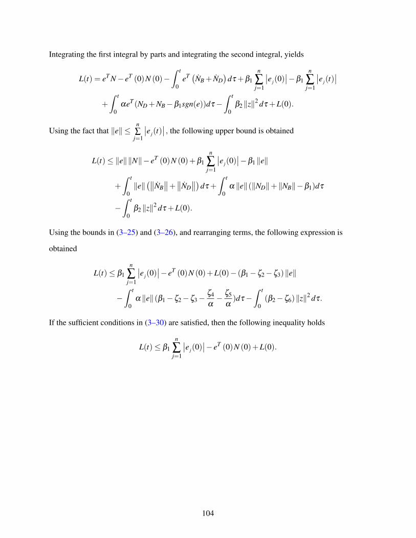
Integrating the first integral by parts and integrating the second integral, yields

L(t) = eT N− eT (0)N (0)−ˆ t

0

eT (NB + ND)

dτ +β1n

∑j=1

∣∣ej(0)∣∣−β1

n

∑j=1

∣∣ej(t)∣∣

+

ˆ t

0

αeT (ND +NB−β1sgn(e))dτ−ˆ t

0

β2 ‖z‖2 dτ +L(0).

Using the fact that ‖e‖ ≤n∑j=1

∣∣ej(t)∣∣ , the following upper bound is obtained

L(t)≤ ‖e‖‖N‖− eT (0)N (0)+β1n

∑j=1

∣∣ej(0)∣∣−β1 ‖e‖

+

ˆ t

0

‖e‖(∥∥NB∥∥+∥∥ND

∥∥)dτ +ˆ t

0

α ‖e‖(‖ND‖+‖NB‖−β1)dτ

−ˆ t

0

β2 ‖z‖2 dτ +L(0).

Using the bounds in (3–25) and (3–26), and rearranging terms, the following expression is

obtained

L(t)≤ β1n

∑j=1

∣∣ej(0)∣∣− eT (0)N (0)+L(0)− (β1−ζ2−ζ3)‖e‖

−ˆ t

0

α ‖e‖(β1−ζ2−ζ3− ζ4α− ζ5

α)dτ−

ˆ t

0

(β2−ζ6)‖z‖2 dτ.

If the sufficient conditions in (3–30) are satisfied, then the following inequality holds

L(t)≤ β1n

∑j=1

∣∣ej(0)∣∣− eT (0)N (0)+L(0).

104

APPENDIX B

DYNAMIC NEURAL NETWORK-BASED GLOBAL OUTPUT FEEDBACK TRACKING

CONTROL FOR UNCERTAIN SECOND-ODER NONLINEAR SYSTEMS

Proof of the Inequality in (5–31)

Integrating (5–30) and using (5–14) yields

H =

ˆ t

0

Ldτ =

ˆ t

0

(rT

es(ND +NB1−β1sgn(x+ν))+ rTtr(ND +NB1−β2sgn(e+ν))

+(·x+ e+2ν)T NB2−β3 ‖z‖2

)dτ.

Using the fact that res =·x+ ν +α(x+ν) and rtr = e+ ν +α(e+ν) yields

H =

ˆ t

0

( ·x+ e+2ν

)T

(ND +NB1+NB2)dτ−ˆ t

0

(·x+ ν)T β1sgn(x+ν)dτ

−ˆ t

0

(e+ ν)T β2sgn(e+ν)dτ +ˆ t

0

α(x+ν)T (ND +NB1−β1sgn(x+ν))dτ

+

ˆ t

0

α(e+ν)T (ND +NB1−β2sgn(e+ν))dτ−ˆ t

0

β3 ‖z‖2 dτ.

Integrating the first integral by parts, and integrating the second and third integrals yields

H = (x+ e+2ν)T N− [x(0)+ e(0)+2ν(0)]T N (0)

+β1n

∑j=1

[∣∣x j(0)+ν j(0)∣∣− ∣∣x j +ν j

∣∣]−ˆ t

0

(x+ e+2ν)T (ND + NB)

dτ

+β2n

∑j=1

[∣∣ej(0)+ν j(0)∣∣− ∣∣ej +ν j

∣∣]−ˆ t

0

β3 ‖z‖2 dτ

+

ˆ t

0

α(e+ν)T [ND +NB1−β2sgn(e+ν)]dτ.

105

Using the fact that ‖x+ν‖ ≤n∑j=1

∣∣x j +ν j∣∣ and ‖e+ν‖ ≤

n∑j=1

∣∣ej +ν j∣∣ , the following upper bound

is obtained

H ≤ ‖x+ e+2ν‖‖N‖− (x(0)+ e(0)+2ν(0))T N (0)

+β1n

∑j=1

∣∣x j(0)+ν j(0)∣∣−β1 ‖x+ν‖

+β2n

∑j=1

∣∣ej(0)+ν j(0)∣∣−β2 ‖e+ν‖

+

ˆ t

0

α ‖x+ν‖∥∥∥∥ND +NB1+

Nα−β1

∥∥∥∥dτ

+

ˆ t

0

α ‖e+ν‖∥∥∥∥ND +NB1+

Nα−β2

∥∥∥∥dτ−ˆ t

0

β3 ‖z‖2 dτ.

Using the bounds in (5–31), based on the fact that ‖x+ e+2ν‖ ≤ ‖x+ν‖+ ‖e+ν‖, andrearranging terms, the following expression is obtained

H ≤ β1n

∑j=1

∣∣x j(0)+ν j(0)∣∣+β2

n

∑j=1

∣∣ej(0)+ν j(0)∣∣

− (x(0)+ e(0)+2ν(0))T N (0)− (β1−ζ2−ζ3−ζ4)‖x+ν‖

− (β2−ζ2−ζ3−ζ4)‖e+ν‖−ˆ t

0

α ‖x+ν‖(β1−ζ2−ζ3− ζ5α− ζ6

α)dτ

−ˆ t

0

α ‖e+ν‖(β2−ζ2−ζ3− ζ5α− ζ6

α)dτ−

ˆ t

0

(β3−2ζ7)‖z‖2 dτ.

If the sufficient conditions in (5–31) are satisfied, then the following inequality holds

H ≤ β1n

∑j=1

∣∣x j(0)+ν j(0)∣∣+β2

n

∑j=1

∣∣ej(0)+ν j(0)∣∣

− (x(0)+ e(0)+2ν(0))T N(0),

H =

ˆ t

0

Ldτ ≤ P(0). (B–1)

Hence, using (5–29) and (B–1), it can be shown that

P(t)≥ 0.

106

REFERENCES

[1] B. Xian, M. S. de Queiroz, D. M. Dawson, and M. McIntyre, “A discontinuous output

feedback controller and velocity observer for nonlinear mechanical systems,” Automatica,vol. 40, no. 4, pp. 695–700, 2004.

[2] L. Vasiljevic and H. Khalil, “Error bounds in differentiation of noisy signals by high-gain

observers,” Systems & Control Letters, vol. 57, no. 10, pp. 856–862, 2008.

[3] D. White and D. Sofge, Handbook of intelligent control: neural, fuzzy, and adaptiveapproaches. Van Nostrand Reinhold Company, 1992.

[4] W. T. Miller, R. Sutton, and P. Werbos, Neural Networks for Control. MIT Press, 1990.

[5] F. L. Lewis, “Nonlinear network structures for feedback control,” Asian J. Control, vol. 1,no. 4, pp. 205–228, 1999.

[6] D. Pham and X. Liu, “Dynamic system identification using partially recurrent neural

networks,” J. Syst. Eng., vol. 2, no. 2, pp. 90–97, 1992.

[7] M. Gupta, L. Jin, and N. Homma, Static and dynamic neural networks: from fundamentalsto advanced theory. Wiley-IEEE Press, 2003.

[8] K. Funahashi and Y. Nakamura, “Approximation of dynamic systems by continuous-time

recurrent neural networks,” Neural Networks, vol. 6, pp. 801–806, 1993.

[9] M. Polycarpou and P. Ioannou, “Identification and control of nonlinear systems using neural

network models: Design and stability analysis,” Systems Report 91-09-01, University ofSouthern California, 1991.

[10] K. Narendra and K. Parthasarathy, “Identification and control of dynamical systems using

neural networks,” IEEE Trans. Neural Networks, vol. 1, no. 1, pp. 4–27, 1990.

[11] E. Kosmatopoulos, M. Polycarpou, M. Christodoulou, and P. Ioannou, “High-order neural

network structures for identification of dynamical systems,” IEEE Trans. Neural Networks,vol. 6, no. 2, pp. 422 – 431, 1995.

[12] G. A. Rovithakis and M. A. Christodoulou, “Adaptive control of unknown plants using

dynamical neural networks,” IEEE Trans. Syst. Man Cybern., vol. 24, pp. 400–412, 1994.

[13] A. Delgado, C. Kambhampati, and K. Warwick, “Dynamic recurrent neural network

for system identification andcontrol,” IEE Proc. Contr. Theor. Appl., vol. 142, no. 4, pp.307–314, 1995.

[14] A. S. Poznyak, W. Yu, E. N. Sanchez, and J. P. Perez, “Nonlinear adaptive trajectory

tracking using dynamic neural networks,” IEEE Trans. Neural Networks, vol. 10, no. 6, pp.1402–1411, Nov 1999.

107

[15] A. Poznyak, E. Sanchez, and W. Yu, Differential neural networks for robust nonlinearcontrol: identification, state estimation and trajectory tracking. World Scientific Pub Co

Inc, 2001.

[16] X. Ren, A. Rad, P. Chan, and W. Lo, “Identification and control of continuous-time

nonlinear systems via dynamic neural networks,” IEEE Trans. Ind. Electron., vol. 50, no. 3,pp. 478–486, 2003.

[17] J. Hopfield, “Neurons with graded response have collective computational properties like

those of two-state neurons,” Proc. Nat. Acad. Sci. U.S.A., vol. 81, no. 10, p. 3088, 1984.

[18] X. Li and W. Yu, “Dynamic system identification via recurrent multilayer perceptrons,” Inf.Sci. Inf. Comput. Sci., vol. 147, pp. 45–63, 2002.

[19] H. Dinh, S. Bhasin, and W. E. Dixon, “Dynamic neural network-based robust identification

and control of a class of nonlinear systems,” in Proc. IEEE Conf. Decis. Control, Atlanta,GA, 2010, pp. 5536–5541.

[20] S. Bhasin, M. Johnson, and W. E. Dixon, “A model-free robust policy iteration algorithm

for optimal control of nonlinear systems,” in Proc. IEEE Conf. Decis. Control, Atlanta, GA,2010, pp. 3060–3065.

[21] J.-J. Slotine, J. Hedrick, and E. A. Misawa, “On sliding observers for nonlinear systems,” in

American Control Conf., 1986, pp. 1794–1800.

[22] C. Canudas De Wit and J.-J. Slotine, “Sliding observers for robot manipulators,” Automat-ica, vol. 27, pp. 859–864, 1991.

[23] M. Mohamed, T. Karim, and B. Safya, “Sliding mode observer for nonlinear mechanical

systems subject to nonsmooth impacts,” in Int. Multi-Conf. Syst. Signals Devices, 2010.

[24] K. W. Lee and H. K. Khalil, “Adaptive output feedback control of robot manipulators using

high-gain observer,” INT. J. CONTROL, vol. 67, pp. 869–886, 1997.

[25] E. Shin and K. Lee, “Robust output feedback control of robot manipulators using high-gain

observer,” in IEEE Int. Conf. on Control and Appl., 1999.

[26] A. Astolfi, R. Ortega, and A. Venkatraman, “A globally exponentially convergent immer-

sion and invariance speed observer for n degrees of freedom mechanical systems,” in Proc.Chin. Control Conf., 2009.

[27] N. Lotfi and M. Namvar, “Global adaptive estimation of joint velocities in robotic manipu-

lators,” IET Control Theory Appl., vol. 4, pp. 2672–2681, 2010.

[28] J. Davila, L. Fridman, and A. Levant, “Second-order sliding-mode observer for mechanical

systems,” IEEE Trans. Autom. Control, vol. 50, pp. 1785–1789, 2005.

[29] D. Dawson, Z.Qu, and J. Carroll, “On the state observation and output feedback problems

for nonlinear uncertain dynamic systems,” Syst. Contr. Lett., vol. 18, pp. 217–222, 1992.

108

[30] Y. H. Kim and F. L. Lewis, “Neural network output feedback control of robot manipula-

tors,” IEEE Trans. Robot. Autom., vol. 15, pp. 301–309, 1999.

[31] H. Berghuis and H. Nijmeijer, “A passivity approach to controller-observer design for

robots,” IEEE Trans. Robot. Autom., vol. 9, pp. 740–754, 1993.

[32] K. D. Do, Z. Jiang, and J. Pan, “A global output-feedback controller for simultaneous

tracking and stabilization for unicycle-type mobile robots,” IEEE Trans. Robot. Autom.,vol. 20, pp. 589–594, 2004.

[33] S. Y. Lim, D. M. Dawson, and K. Anderson, “Re-examining the nicosia-tomei robot

observer-controller for a backstepping perspective,” IEEE Trans. Control Syst. Technol.,vol. 4, pp. 304–310, 1996.

[34] M. A. Arteaga and R. Kelly, “Robot control without velocity measurements: New theory

and experiment results,” IEEE Trans. Robot. Autom., vol. 20, pp. 297–308, 2004.

[35] K. Kaneko and R. Horowitz, “Repetitive and adaptive control of robot manipulators with

velocity estimation,” IEEE Trans. Robot. Autom., vol. 12, pp. 204–217, 1997.

[36] T. Burg, D. Dawson, J. Hu, and M. de Queiroz, “An adaptive partial state feedback

controller for rled robot manipulators,” IEEE Trans. Autom. Control, vol. 41, pp. 1024–1031, 1996.

[37] T. Burg, D. M. Dawson, and P. Vedagarbha, “A redesigned dcal controller without velocity

measurements: Theory and demonstration,” Robotica, vol. 15, no. 4, pp. 337–346, 1997.

[38] F. Zhang, D. M. Dawson, M. S. de Queiroz, and W. E. Dixon, “Global adaptive output

feedback tracking control of robot manipulators,” IEEE Trans. Automat. Control, vol. 45,pp. 1203–1208, 2000.

[39] S. Seshagiri and H. Khalil, “Output feedback control of nonlinear systems using rbf neural

networks,” IEEE Trans. Neural Netw., vol. 11, pp. 69–79, 2000.

[40] J. Y. Choi and J. A. Farrell, “Adaptive observer backstepping control using neural network,”

IEEE Trans. Neural Netw., vol. 12, pp. 1103–1112, 2001.

[41] A. J. Calise, N. Hovakimyan, and M. Idan, “Adaptive output feedback control of nonlinear

systems using neural networks,” Automatica, vol. 37, no. 8, pp. 1201–1211, 2001.

[42] N. Hovakimyan, F. Nardi, A. Calise, and N. Kim, “Adaptive output feedback control of

uncertain nonlinear systems using single-hidden-layer neural networks,” IEEE Trans.Neural Networks, vol. 13, no. 6, pp. 1420–1431, Nov. 2002.

[43] S. Islam and P. Liu, “Robust adaptive fuzzy output feedback control system for robot

manipulators,” IEEE/ASME Trans. Mechatron., vol. 16, pp. 288–296, 2011.

[44] J. A. Cook and B. K. Powell, “Modeling of an internal combustion engine for control

analysis,” IEEE Control Syst. Mag, pp. 20–25, 1988.

109

[45] M. Kao and J. J. Moskwa, “Turbocharged diesel engine modeling for nonlinear engine

control and state estimation,” ASME J. Dyn. Syst., Meas., Control, vol. 117, pp. 20–30,1995.

[46] F. L. Lewis, R. Selmic, and J. Campos, Neuro-Fuzzy Control of Industrial Systems withActuator Nonlinearities. Philadelphia, PA, USA: Society for Industrial and Applied

Mathematics, 2002.

[47] G. Niemeyer and J.-J. Slotine, “Telemanipulation with time delays,” Int. J. Robot. Res.,vol. 23, pp. 873–890, 2004.

[48] A. Aziminejad, M. Tavakoli, R. V. Patel, and M. Moallem, “Stability and performance in

delayed bilateral teleoperation: Theory and experiments,” Control Eng. Pract., vol. 16, pp.1329–1343, 2008.

[49] Y. Gu, C. Zhang, and K. T. Chong, “Adaptive passive control with varying time delay,”

Simul. Model. Pract. Theory, vol. 18, pp. 1–8, 2010.

[50] F. Hashemzadeh, I. Hassanzadeh, M. Tavakoli, and G. Alizadeh, “Adaptive control for

state synchronization of nonlinear haptic telerobotic systems with asymmetric varying time

delays,” J. Intell. Robot. Syst., 2012.

[51] N. N. Krasovskii, Stability of motion. Stanford University Press, 1963.

[52] X. Li and C. de Souza, “Delay-dependent robust stability and stabilization of uncertain

linear delay systems: a linear matrix inequality approach,” IEEE Trans. Autom. Control,vol. 42, no. 8, pp. 1144–1148, Aug 1997.

[53] V. B. Kolmanovskii, S.-I. Niculescu, and J.-P. Richard, “On the liapunov-krasovskii

functionals for stability analysis of linear delay systems,” Int. J. Control, vol. 72, pp. 374 –384, 1999.

[54] B. S. Razumikhin, “On the stability of systems with a delay,” Prikl. Mat. Meh, vol. 20, pp.500–512, 1956.

[55] ——, “Application of liapunov’s method to problems in the stability of systems with a

delay,” Automat. i Telemeh, vol. 21, pp. 740–749, 1960.

[56] M. Jankovic, “Control Lyapunov-Razumikhin functions and robust stabilization of time

delay systems,” IEEE Trans. Autom. Control, vol. 46, no. 7, pp. 1048–1060, 2001.

[57] R. Bellman and K. L. Cooke, Differential- Difference Equations. Academic Press, 1963.

[58] L. E. Elsgolts and S. B. Norkin, Introduction to the theory and application of differentialequations with deviating arguments. Academic Press, 1973, vol. 105.

[59] F. Mazenc, S. Mondie, R. Francisco, P. Conge, I. Lorraine, and F. Metz, “Global asymptotic

stabilization of feedforward systems with delay in the input,” IEEE Trans. Autom. Control,vol. 49, (5), pp. 844–850, 2004.

110

[60] B. Chen, X. Liu, and S. Tong, “Robust fuzzy control of nonlinear systems with input delay,”

Chaos, Solitons & Fractals, vol. 37, no. 3, pp. 894–901, 2008.

[61] M. Krstic, “Input delay compensation for forward complete and strict-feedforward

nonlinear systems,” IEEE Trans. Autom. Control, vol. 55, pp. 287–303, feb. 2010.

[62] B. Castillo-Toledo, S. Di Gennaro, and G. Castro, “Stability analisys for a class of sampled

nonlinear systems with time-delay,” in Proc. IEEE Conf. Decis. Control, 2010, pp. 1575–1580.

[63] N. Sharma, S. Bhasin, Q. Wang, and W. E. Dixon, “Predictor-based control for an uncertain

Euler-Lagrange system with input delay,” Automatica, vol. 47, no. 11, pp. 2332–2342,2011.

[64] L. Guo, “H infin; output feedback control for delay systems with nonlinear and parametric

uncertainties,” Proc. IEE Control Theory Appl., vol. 149, no. 3, pp. 226 –236, 2002.

[65] W. Li, Y. Dong, and X. Wang, “Robust h infin; control of uncertain nonlinear systems

with state and input time-varying delays,” in Proc. Chin. Control Decis. Conf., 2010, pp.317–321.

[66] N. Bekiaris-Liberis and M. Krstic, “Compensation of time-varying input delay for nonlinear

systems,” inMediterr. Conf. Control and Autom., Corfu, Greece, 2011.

[67] M. Krstic, “Lyapunov stability of linear predictor feedback for time-varying input delay,”

IEEE Trans. Autom. Control, vol. 55, pp. 554–559, 2010.

[68] N. Fischer, R. Kamalapurkar, N. Fitz-Coy, and W. E. Dixon, “Lyapunov-based control of

an uncertain Euler-Lagrange system with time-varying input delay,” in American ControlConference, Montréal, Canada, June 2012, pp. 3919–3924.

[69] A. Ailon and M. Gil, “Stability analysis of a rigid robot with output-based controller and

time delay,” Systems & Control Letters, vol. 40, no. 1, pp. 31–35, 2000.

[70] A. Ailon, R. Segev, and S. Arogeti, “A simple velocity-free controller for attitude regulation

of a spacecraft with delayed feedback,” IEEE Trans. Autom. Control, vol. 49, no. 1, pp.125–130, 2004.

[71] A. Ailon, “Asymptotic stability in a flexible-joint robot with model uncertainty and multiple

time delays in feedback,” J. Franklin Inst., vol. 341, no. 6, pp. 519–531, 2004.

[72] A. Poznyak, W. Yu, E. Sanchez, and H. Sira-Ramirez, “Robust identification by dynamic

neural networks using sliding mode learning,” Appl. Math. Comput. Sci., vol. 8, pp. 135–144, 1998.

[73] J. Huang and F. Lewis, “Neural-network predictive control for nonlinear dynamic systems

with time-delay,” IEEE Trans. Neural Networks, vol. 14, no. 2, pp. 377–389, 2003.

111

[74] B. Xian, D. M. Dawson, M. S. de Queiroz, and J. Chen, “A continuous asymptotic tracking

control strategy for uncertain nonlinear systems,” IEEE Trans. Autom. Control, vol. 49, pp.1206–1211, 2004.

[75] P. M. Patre, W. MacKunis, K. Kaiser, and W. E. Dixon, “Asymptotic tracking for uncertain

dynamic systems via a multilayer neural network feedforward and RISE feedback control

structure,” IEEE Trans. Automat. Control, vol. 53, no. 9, pp. 2180–2185, 2008.

[76] H. T. Dinh, R. Kamalapurkar, S. Bhasin, and W. E. Dixon, “Dynamic neural network-based

robust observers for second-order uncertain nonlinear systems,” in Proc. IEEE Conf. Decis.Control, Orlando, FL, 2011, pp. 7543–7548.

[77] H. T. Dinh, S. Bhasin, D. Kim, and W. E. Dixon, “Dynamic neural network-based global

output feedback tracking control for uncertain second-order nonlinear systems,” in AmericanControl Conference, Montréal, Canada, June 2012, pp. 6418–6423.

[78] S. Haykin, Neural Networks and Learning Machines, 3rd ed. Upper Saddle River, NJ:

Prentice Hall, 2008.

[79] D. R. Hush and B. G. Horne, “Progress in supervised neural networks,” IEEE SignalProcess. Mag., vol. 10, no. 1, pp. 8–39, 1993.

[80] J. Hopfield, “Neural networks and physical systems with emergent collective computational

abilities,” in Proc. Nat. Acad. Sci. USA, vol. 79, 1982, pp. 2554–2558.

[81] E. Sontag, “Neural nets as system models and controllers,” in Proc. 7th Yale workshop onAdaptive and Learning Systems, 1992, pp. 73–79.

[82] I. Sandberg, “Approximation theorems for discrete-time systems,” IEEE Trans. on Circuitsand Syst., vol. 38, pp. 564–566, 1991.

[83] ——, “Uniform approximation and the circle criterion,” IEEE Trans. on Autom. Control,vol. 38, pp. 1450–1458, 1993.

[84] ——, “Uniform approximation of multidimensional myopic maps,” IEEE Trans. on Circuitsand Syst., vol. 44, pp. 477–485, 1997.

[85] K. Hornick, “Approximation capabilities of multilayer feedforward networks,” NeuralNetworks, vol. 4, pp. 251–257, 1991.

[86] G. Cybenko, “Approximation by superpositions of a sigmoidal function,” Math. ControlSignals Syst., vol. 2, pp. 303–314, 1989.

[87] A. Barron, “Universal approximation bounds for superpositions of a sigmoidal function,”

IEEE Trans. Inf. Theory, vol. 39, no. 3, pp. 930–945, 1993.

[88] W. E. Dixon, A. Behal, D. M. Dawson, and S. Nagarkatti, Nonlinear Control of EngineeringSystems: A Lyapunov-Based Approach. Birkhäuser: Boston, 2003.

112

[89] M. Krstic, P. V. Kokotovic, and I. Kanellakopoulos, Nonlinear and Adaptive Control Design.John Wiley & Sons, 1995.

[90] P. M. Patre, W. Mackunis, C. Makkar, and W. E. Dixon, “Asymptotic tracking for systems

with structured and unstructured uncertainties,” IEEE Trans. Control Syst. Technol., vol. 16,pp. 373–379, 2008.

[91] A. Filippov, “Differential equations with discontinuous right-hand side,” Am. Math. Soc.Transl., vol. 42 no. 2, pp. 199–231, 1964.

[92] A. F. Filippov, Differential Equations with Discontinuous Right-hand Sides. Kluwer

Academic Publishers, 1988.

[93] G. V. Smirnov, Introduction to the theory of differential inclusions. American MathematicalSociety, 2002.

[94] J. P. Aubin and H. Frankowska, Set-valued analysis. Birkhäuser, 2008.

[95] R. Leine and N. van de Wouw, “Non-smooth dynamical systems,” in Stability andConvergence of Mechanical Systems with Unilateral Constraints, ser. Lecture Notes inApplied and Computational Mechanics. Springer Berlin / Heidelberg, 2008, vol. 36, pp.

59–77.

[96] F. H. Clarke, Optimization and nonsmooth analysis. SIAM, 1990.

[97] D. Shevitz and B. Paden, “Lyapunov stability theory of nonsmooth systems,” IEEE Trans.Autom. Control, vol. 39 no. 9, pp. 1910–1914, 1994.

[98] B. Paden and S. Sastry, “A calculus for computing Filippov’s differential inclusion with

application to the variable structure control of robot manipulators,” IEEE Trans. CircuitsSyst., vol. 34 no. 1, pp. 73–82, 1987.

113

BIOGRAPHICAL SKETCH

Huyen T. Dinh was born in April, 1984 in Thai Nguyen, Vietnam. She received her

Bachelor of Engineering degree in Mechatronic Engineering in 2006 from Hanoi University of

Technology (HUT), Vietnam. She worked as a lecturer in Mechanical Engineering department of

University of Transport and Communications, Vietnam from September 2006. She then joined

the Nonlinear Controls and Robotics (NCR) research group at the University of Florida (UF)

to pursue her doctoral research under the advisement of Dr. Warren Dixon since August 2008

and completed her Ph.D. in August 2012. From September 2012 onward she will be an assistant

professor in the University of Transport and Communications, Vietnam.

114

DYNAMIC NEURAL NETWORK-BASED ROBUST CONTROL …ncr.mae.ufl.edu/dissertations/huyen.pdf · dynamic...

Documents

Transcript of DYNAMIC NEURAL NETWORK-BASED ROBUST CONTROL …ncr.mae.ufl.edu/dissertations/huyen.pdf · dynamic...