The University of Maine The University of Maine

DigitalCommons@UMaine DigitalCommons@UMaine

Honors College

Spring 5-2016

Dynamic Modeling of a Catamaran Using a Lagrangian Approach Dynamic Modeling of a Catamaran Using a Lagrangian Approach

Tamara R. Thomson

Follow this and additional works at: https://digitalcommons.library.umaine.edu/honors

Part of the Mechanical Engineering Commons

Recommended Citation Recommended Citation Thomson, Tamara R., "Dynamic Modeling of a Catamaran Using a Lagrangian Approach" (2016). Honors College. 419. https://digitalcommons.library.umaine.edu/honors/419

This Honors Thesis is brought to you for free and open access by DigitalCommons@UMaine. It has been accepted for inclusion in Honors College by an authorized administrator of DigitalCommons@UMaine. For more information, please contact um.library.technical.services@maine.edu.

DYNAMIC MODELING OF A CATAMARAN USING A LAGRANGIAN APPROACH

by

Tamara R. Thomson

A Thesis Submitted in Partial Fulfillment

of the Requirements for a Degree with Honors (Mechanical Engineering)

The Honors College

University of Maine

May 2016

Advisory Committee: Michael “Mick” Peterson, Professor of Mechanical Engineering Sergey Lvin, PhD, Lecturer of Mathematics Margaret O. Killinger, PhD, Associate Professor and Rezendes Preceptor for the Arts Murray Callaway, Lecturer of English Zhihe Jin, PhD, Associate Professor of Mechanical Engineering

© 2016 Tamara Thomson All Rights Reserved

Abstract

In this thesis, the development and application of a dynamic model of the 2016

Autonomous Boat Team’s catamaran are discussed. The model is two dimensional and

describes the motion of the boat in a calm freshwater environment. The linear and

rotational equations of motion used in the model were derived by employing Lagrangian

dynamics, and the thrust of the motors and drag of the hulls were found through

experimentation. The resulting equations are  𝑚𝑎 = !!∙ 𝜌 ∙ 𝑥!𝐶!"𝐴 + 2𝐹 and 𝐼𝛼 = !

!"∙ 𝜌 ∙

𝜃!𝐶!"𝐴 + 𝐹! ∙!!− 𝐹! ∙

!!. The thrust and drag here vary with respect to voltage and

velocity.

The following document is organized to first supply the reader with background

information sufficient to understand the project’s purpose and merits and then discuss the

experiments and derivations necessary for completing the objectives. Next, the resulting

model is presented and discussed at length followed by a section about the applications

and future work suggestions for this project.

vi

This thesis is dedicated to my family, Stacy, Randall, and

Anthony Thomson.

vii

Acknowledgements

I would like to acknowledge the contributions made by my entire thesis

committee, most notably Dr. Mick Peterson, my thesis advisor. Thank you for all the

help and support you’ve given me throughout my undergraduate experience.

Additionally, I’d like to acknowledge the work contributed by my capstone team

that was critical for the completion of this thesis. Riley Mattor, Chris Derr, and Ben

Dickinson were extremely helpful and surprisingly willing to assist me at every stage of

this project. Thank you.

viii

Table of Contents

Abstract ................................................................................................................................ 3

Introduction ......................................................................................................................... 1 Objectives ........................................................................................................................ 2 Scope of Project ............................................................................................................... 2 Dynamics – History and Options ..................................................................................... 5

Methods and Analysis ......................................................................................................... 7 Derivation of the Equations of Derivation of the Equations of Motion .......................... 8 Conducting the Drag Experiment .................................................................................. 11 Conducting the Thrust Curve Experiment ..................................................................... 13 Constructing the Model .................................................................................................. 16

Results ............................................................................................................................... 17 Equations of Motion ...................................................................................................... 17 Drag ................................................................................................................................ 17 Thrust Curves ................................................................................................................. 20 Model ............................................................................................................................. 22

Conclusions and Future Work ........................................................................................... 24

Bibliography ...................................................................................................................... 26

APPENDIX A .................................................................................................................... 27

APPENDIX B .................................................................................................................... 28

APPENDIX C .................................................................................................................... 29

APPENDIX D .................................................................................................................... 30

Author’s Biography ........................................................................................................... 31

ix

Table of Figures Figure 1 SolidWorks diagram of catamaran ........................................................................ 1

Figure 4 Diagram of drag testing setup ............................................................................. 12

Figure 5 Minn Kota motor with trim lever secured open and load cell in line with tether14

Figure 6 Free body diagram of trolling motor during test ................................................. 15

Figure 7 Predicted drag curve depicting the drag calculated using Equation 15 for each velocity ...................................................................................................................... 18

Figure 8 Drag curve using measured data ......................................................................... 18

Figure 9 Forward thrust curve for motor 1 ........................................................................ 20

Figure 10 Forward thrust curve for motor 2 ...................................................................... 20

Figure 11 Reverse thrust curve for motor 1 ....................................................................... 21

Figure 12 Reverse thrust curve for motor 2 ....................................................................... 21

Figure 13 Predicted linear velocity of the catamaran ........................................................ 23

Figure 14 Predicted angular velocity of the catamaran ..................................................... 23

1

Introduction

This thesis describes the efforts employed in the development of a model to

predict the movement of a catamaran in a calm freshwater environment and displays the

results. To help reader understand the scope of the undertaking this was, the thesis

begins with a description of the catamaran in question. The catamaran whose motion is

described with this model is the 2016 Autonomous Boat Team’s capstone project. It is

16.5 feet in length and 8.5 feet wide, measured from the points of the pontoons. The

catamaran is driven by two Minn Kota trolling motors (model number C2 30) attached

directly behind the pontoons. A labeled diagram of the catamaran is displayed below in

Figure 1.

Figure 1 SolidWorks diagram of catamaran

16.5’ 8.5’

Motors

2

Objectives

The overall objective of this undertaking was to create a dynamic model of a

catamaran. In order to complete this model, several intermediate objectives had to be

met. Those objectives are listed below.

• Analytically determine the equations of motion for the catamaran using

Lagrangian dynamics.

• Experimentally determine the drag coefficient associated with the catamaran in

fresh water.

• Create thrust curves for the motors using experimental data.

• Determine the moment of inertia of the catamaran using a SolidWorks model.

Each of the objectives listed above was essential for the completion of the model.

Without accurately measured criteria, the model would be inaccurate, and without

correctly derived equations of motion, even the most accurate experimental data is moot.

Scope of Project

This thesis is a portion of a larger capstone project that was undertaken

simultaneously by the 2016 Autonomous Boat Team. In order to clarify the value of

completing a dynamic model of the catamaran, it is necessary to explain the background

of the capstone project itself.

Hydroelectric energy is the largest form of renewable energy in the United States,

providing approximately 96% of the renewable energy consumed by our country in 2005

[1]. New sources of hydroelectric energy are continually being sought. Generators placed

in dams are reliable and effective energy sources, but damming flowing water is not

always a viable option in populated or protected regions.

3

The ocean presents an enormous amount of harnessable energy in its tides.

Unlike sources of solar and wind energy, tidal energy is very dependable; the tides

operate on reliable schedules all year long. It is widely known that the tides are largely

caused by the gravitational attraction between the earth and the moon, meaning that tidal

energy cannot be overdrawn and will not fail.

Maine has some of the largest tidal ranges in the world. The highest recorded on

earth are in the Bay of Fundy which is located in the Gulf of Maine. Here, the tidal range

reaches up to 50 feet [2]. Tidal ranges such as this are uncommon, but other areas on the

coast of Maine have relatively high tidal ranges as well. The tidal range in Cobscook

Bay, a shallow estuary in Downeast Maine, averages 24 feet [3], which is much smaller

than that of the Bay of Fundy, but is eight time the average world-wide [2]. Bays with

high tidal ranges produce large currents, providing the potential for collection of large

amounts of energy. Ocean Renewable Power Company (ORPC) recognized this potential

and developed and installed a tidal turbine in Cobscook Bay. However, several factors

had to be considered before installation was possible.

The Cobscook Bay area is home to about 7,000 people, many of whom are

fishermen that depend on the health of the fishery for their livelihoods [3]. The

population of fish is not only crucial to the inhabitants in the area. It is also vital to the

fragile ecosystem in Cobscook Bay and the entire Gulf of Maine that the fish remain

unharmed. As Michael Johnson writes,

4

The area is home to important fish species such as Atlantic herring, winter flounder, Atlantic cod, and haddock, as well as anadromous fish including alewife, blueback herring, and rainbow smelt. These anadromous fish live within the Cobscook Bay estuary until they reach maturity, and then make annual spawning migrations into the freshwater rivers and streams that flow into the bay. They serve as food for larger species, including Atlantic cod, haddock, bluefin tuna, bluefish, sea birds, and marine mammals like seals. Cobscook Bay is also a vital center for Maine’s aquaculture because it provides prime habitat for sea scallops, sea urchins, and soft-shelled clams.

[3]

Such valuable ecological resources need to be protected both for the good of the local

economy and the environment. Understanding this, ORPC placed in Cobscook Bay a

platform designed by the Northeastern Regional Association of Coastal Ocean Observing

Systems (NERACOOS), equipped with hydro-acoustic sensors to monitor the movements

and migration patterns of the indigenous community of fish. The goal was to collect data

to determine if a turbine could be installed without harming wildlife in the bay. More

specifically, the intent was to determine if the installation would negatively impact the

population of fish. Activity in the area directly around the NERACOOS platform would

compare multi-year base line data with data obtained after the installation of ORPC’s

turbine. An adaptive management plan would then require mitigation of the impact or

even removal of the turbine if its effects were excessive. The data set required for this

effort is significant because because of the influence of annual variations in the fish

population. The cost and complexity of this monitoring is a significant barrier to the

adoption of tidal energy generation. The large amount of hydro-acoustic data obtained

from the monitoring would require large amounts of data to be obtained over long periods

of time.

5

The goal of the 2016 Autonomous Boat Team’s capstone project was to design,

build, and program a prototype of a boat that could autonomously navigate to the GPS

coordinates of the NERACOOS platform and make a physical connection with an

offshoot buoy, collecting the data and providing power when necessary. The physical

connection was essential because of the large amounts of data being collected by the

hydro-acoustic sensors weekly – several terabytes. It is also essential because the boat is

intended to help recharge the batteries to supply the high power demand of the platform.

This is especially necessary during periods of the year when solar power is limited. The

completion of this boat would provide relief for workers collecting data year round. This

would also significantly reduce the cost of collecting the data from the offshore platform.

Any vehicle is difficult to automate, and this catamaran was no exception. It was

essential to understand how the catamaran reacted when voltage was supplied to its

motors so it could be programmed to navigate to the NERACOOS platform unmanned.

The model created for the completion of this thesis was designed to describe the motion

of the boat in calm water, which is a stepping stone to the creation of a model that would

describe the motion of the catamaran at sea, with applied waves and currents. The model

described here was implemented in the catamaran prototype which was merely a proof of

concept never intended to be operated in choppy water or without supervision.

Dynamics – History and Options

Dynamics is the study of moving bodies. Lagrangian mechanics has been

employed to create the model presented in this thesis. In an effort to shed some light on

6

the decision to use Lagrangian mechanics, a brief explanation of the development of

Newtonian and Lagrangian dynamics will be provided in this section.

As Sir Isaac Newton said in the preface to the Principia, “mechanics will be the science

of motion resulting from any forces whatsoever, and of the forces required to produce

any motion” [4]. This quote gives the reader an idea of the breadth and value of

dynamics.

Newton is the father of Newtonian dynamics, also called vectorial mechanics and

the direct approach, which is commonly taught in undergraduate classrooms today.

Newtonian dynamics relies on Newton’s famous three laws. Jakob Bernoulli later

discovered that solutions to dynamic problems could be solved for by balancing forces

and moments. It was Euler who first recognized and wrote these equations: 𝐹! =

𝑚𝑎!,    𝐹! = 𝑚𝑎!,    𝐹! = 𝑚𝑎!. Later, Euler discovered and published his First and Second

Axioms, which defined linear and angular momentum. With this advancement, finally

classical mechanics was born, and it has changed very little since 1776 [5].

Another approach based on energy and work exists, Lagrangian dynamics. This

approach is also called the indirect approach and analytical dynamics. Famous German

mathematician and philosopher Gottfried Leibniz was the first recorded believer in the

indirect method. In the 1600’s Leibniz theorized that there were “living” and “dead”

forces, and he believed that changes in these forces could be related to work done in a

system. Nearly two centuries later, Lagrange and Euler studied the principle of least

7

action and developed hypotheses about kinetic and potential energy. In 1788, Lagrange

published Mecanique Analytique, giving birth to Lagrangian mechanics [5].

The histories of these two methods are enlightening. They outline the work that

went into their development and touch on some important aspects of the two methods that

should be considered before deciding which is best applied to certain systems. Both

approaches generate the same answers, but more steps are often required for problem

solving in Newtonian mechanics. Newtonian mechanics is a more intuitive process; the

effects of forces and moments can be observed. Energy, on the other hand, is a nebulous

concept until it is fully grasped. The beauty of this indirect method, though, is that all

components are scalar, giving Lagrangian mechanics the hefty advantage of having

generalized coordinates. No matter how the coordinates of a system are oriented or how

they change, Lagrange’s methods do not vary. It is for this reason that Lagrangian

dynamics was selected for derivation of this model. In this case the combined angular

and linear motion of the boat is easily combined into two equations of motion.

Methods and Analysis

This thesis combines analysis and experimental testing. Finding the equations of

motion of the catamaran required an analytical derivation using Lagrangian dynamics.

The thrust curves of the engines were then

found experimentally, as was the drag

force on the boat. The coefficient of drag,

Figure 2 Flowchart of inputs for model

8

necessary to predict the drag induced by traveling at a range of velocities, was then found

from additional analysis. Figure 3 shows a schematic flowchart of the experimental and

analytical results and how they relate to the model. The process by which each of these

components were developed is outlined in the following sections of the document.

Derivation of the Equations of Derivation of the Equations of Motion

The application of a Lagrangian formulation of the

equations of motion using linear and rotational terms was

relatively simple. The methodology was easily able to

address the complexities of the problem. This thesis work

included learning how to derive the equations of motion

using a Lagrangian method which is not a part of the

undergraduate engineering curriculum at UMaine. It was

necessary to build a foundation of knowledge of the

process with less complex problems prior to tackling this one. This previous study

provided a clear understanding of the proper steps necessary to complete the derivation of

the equations of motion. Before analysis began, a free body diagram (FBD) of the

system was drawn (Figure 3).

To complete this solution, the steps in Fundamentals of Applied Dynamics were followed

[6]. The first step in this process was to define the generalized coordinates used in the

system. This is done below.

Figure 3 FBD of catamaran

9

𝜉! = 𝑥,𝜃                      𝜕𝜉 = 𝜕𝑥,𝜕𝜃

The next step is to define generalized forces. The system analyzed here, the catamaran,

does not include any conservative forces. The generalized forces nonconservative work

is

𝜕𝑊|!" = !!𝜕𝜃 𝐷! + 𝐹! 𝜕𝑥

!!𝐷!! − 𝐹! 𝜕𝑥 !

!𝐷!! + (𝐹! + 𝐹!)𝜕𝑥 (Eq. 1)

where 𝑊|!" is the nonconservative work completed by the forces acting on the

catamaran. The rotational coordinate is  𝜃, and 𝑥 is the translational coordinate. The

distance between the pontoons is 𝑏. 𝐷!! is the force of drag induced by pontoon two

moving backward, and 𝐷!! is the force of drag induced by pontoon one moving forward.

The entire drag induced when the boat is turning is 𝐷! = !!(𝐷!! + 𝐷!!). Thrust of the

motors is represented by  𝐹! and 𝐹!, respectively.

The equation for drag (Equation 2) is commonplace and can be referenced from any fluid

mechanics book. The author references Fundamentals of Fluid Mechanics [7].

𝐷! =!!𝜌 ∙ 𝑉! ∙ 𝐶! ∙ 𝐴 (Eq. 2)

In Equation 2, 𝜌 is the density of water, 65.55 !!"!"!

[7], 𝑉 is the velocity of the catamaran,

𝐶! is the drag coefficient of the pontoons, and 𝐴 is the cross-sectional area of the

pontoons.

The drag equation can be expanded by elaborating on velocity.

𝐷! =!!𝜌 ∙ (!

!𝜃)! ∙ 𝐶! ∙ 𝐴 (Eq. 3)

10

Inserting Equation 3 into Equation 1 yields Equation 4.

𝜕𝑊|!" =𝑏2 𝜕𝜃

12𝜌 ∙

𝑏2 𝜃

!

∙ 𝐶! ∙ 𝐴 + 𝐹! 𝜕𝑥𝑏2 𝐷!! −

(𝐹!)(𝜕𝑥)(!!)𝐷!! + (𝐹! + 𝐹!)𝜕𝑥 (Eq. 4)

The next step outlined by Williams is to define the Lagrangian term. The Lagrangian is

defined as the kinetic energy of a system, 𝑇, minus the potential, 𝑈. For this application,

there is no potential energy. Therefore, 𝑈 = 0. The kinetic energy of this system is

shown in Equation 5.

𝑇 = !!∙ 𝐼 ∙ 𝜃! + !

!𝑚 ∙ 𝑥! (Eq. 5)

𝐼 is the moment of inertia, 𝜃 is the rotational velocity, 𝑚 is the mass of the catamaran,

and 𝑥 is the linear velocity.

The resulting Lagrangian then is the kinetic energy of the system. This is shown in

Equation 6.

ℒ = !!∙ 𝐼 ∙ 𝜃! + !

!𝑚 ∙ 𝑥! (Eq. 6)

Next is step four, employing Lagrange’s equation. Lagrange’s equation is seen below in

Equation 7.

!!"

!ℒ!!!+ !ℒ

�!!= Ξ! (Eq. 7)

Remembering back to the generalized coordinate definitions, 𝜕𝜉 = 𝜕𝑥,𝜕𝜃. Now,

Lagrange’s equation can be evaluated for the two generalized coordinates of this system.

!!"

!ℒ!!+ !ℒ

!"= Ξ! = 𝑚𝑥 = !

!∙ 𝜌 ∙ 𝑥!𝐶!"𝐴 + 2𝐹 (Eq. 8)

!!"

!ℒ!!+ !ℒ

!"= Ξ! = 𝐼𝜃 = !

!"∙ 𝜌 ∙ 𝜃!𝐶!"𝐴 + 𝐹! ∙

!!− 𝐹! ∙

!! (Eq. 9)

The partial derivative of nonconservative work can be defined as shown in Equation 10.

11

𝜕𝑊|!" = Ξ! ∙ 𝜕𝑥 + Ξ! ∙ 𝜕𝜃 (Eq. 10)

Expanding by inserting Ξ! and Ξ! yields Equation 11.

𝜕𝑊|!" = (!!∙ 𝜌 ∙ 𝑥!𝐶!"𝐴 + 2𝐹) ∙ 𝜕𝑥 + (

!!"∙ 𝜌 ∙ 𝜃!𝐶!"𝐴 + 𝐹! ∙

!!− 𝐹! ∙

!!) ∙ 𝜕𝜃 (Eq. 11)

Since 𝑥 is linear acceleration, and 𝜃 is angular acceleration, the translational and

rotational components can be rewritten:

𝑚𝑎 = !!∙ 𝜌 ∙ 𝑥!𝐶!"𝐴 + 2𝐹 (Eq. 12)

𝐼𝛼 = !!"∙ 𝜌 ∙ 𝜃!𝐶!"𝐴 + 𝐹! ∙

!!− 𝐹! ∙

!! (Eq. 13)

Equation 12 and 13 are the equations of motion which describe the system.

Conducting the Drag Experiment

There are several kinds of drag: form drag, pressure drag, and frictional drag. For

the purposes of this project, all significant forms of drag were lumped together to create

one drag term that could be measured.

To find the drag force on the catamaran, the catamaran was launched in a body of

water and tied behind another boat. A spring scale was attached in line between the

catamaran and the towing boat in such a way as to allow for a member of the group to

collect measurements from it. A GPS was located on the towing boat and was used to

collect the speed of the two crafts during the experiment. A diagram of the testing setup

is included below in Figure 4 for clarity.

12

Figure 2 Diagram of drag testing setup

Before testing began, the speed of the current was determined using the GPS by

allowing the boat to float downstream with no motor activity. The current speed was

found to be 0.4 mph, and from this point on data were collected only while the catamaran

was being towed upstream.

To find the drag force, the catamaran was towed through the water at a constant

speed which was documented along with the measurement given by the spring scale for

each run. This was repeated ten times. The raw data collected during the test are

displayed in Appendix A.

To evaluate the validity of the calculations, the drag force was also measured

while varying the boat speed. Using the same method described above, the drag on the

pontoons was observed while varying the velocity from 1 mph to 5 mph. The raw data

collected during this portion of testing are included in Appendix A.

Data analysis began with a correction for the velocity of the current. Since the catamaran

was always being towed upstream, the current of the river was added to the velocity of

each run.

The drag force was created by towing the boat at one speed which was measured

during the experiment. In order to be able to predict the drag force at different velocities

13

for use in a dynamic model. A coefficient of drag must be determined. Using the drag

force and speed measured during the experiment the drag coefficient was determined.

The force is defined using Equation 14.

𝐹! =!!∙ 𝜌 ∙ 𝐴 ∙ 𝐶! ∙ 𝑉! (Eq. 14)

In this application 𝐹! is the drag force which was collected experimentally using a spring

scale, 𝐴 is the cross-sectional area of the pontoons in 𝑓𝑡!, 𝐶! is the coefficient of drag,

which is dimensionless, and 𝑉 is the velocity at which the boat is travelling in !"!

.

Because the cross-sectional area of the boat and the drag coefficient do not

change, they can be combined to form one constant that will be defined as 𝐶!". Thus, the

equation is slightly simplified. It is displayed below as Equation 15.

𝐹! =!!∙ 𝜌 ∙ 𝐶!" ∙ 𝑉! (Eq. 15)

Since every term in Equation 15 is known, it is possible to solve for 𝐶!". The combined

coefficient of drag and cross-sectional area is used to calculate an array of drag forces by

varying the velocity of the catamaran. The final equation for the coefficient of drag is

Equation 16.

𝐶!" =!∙!!!∙!!

(Eq. 16)

Conducting the Thrust Curve Experiment

The goal of this experiment was to generate thrust curves for the two Minn Kota

motors used for the 2016 Autonomous Boat. Each motor was tested individually. The

test began with the motor suspended from an immobile gantry over a tank of water. The

14

lever that allows rotation of the motor around its mount was fixed in the open position,

and the shaft of the motor was tethered to a rigid beam. An Omega LCCD-100 load cell

was secured in line between the rigid beam and the motor shaft. The data sheet for the

Omega LCCD-100 is in Appendix B. The distances between the pivot point and the load

cell and the load cell and the propeller along the shaft were measured and recorded. As

voltage is supplied to the motor, the propeller spins creating thrust, and a force can be

measured by the load cell. Figure 5 is a diagram of the motor setup.

Figure 3 Minn Kota motor with trim lever secured open and load cell in line with tether

The load cell was wired to an Omega DP25-S-A display that displayed the measured

force in lbf based on a voltage output from the load cell.

15

Each of the motors was wired though a Sabertooth 2X60 motor controller to an Arduino.

When the Arduino emitted a Pulse Width Modulation (PWM) signal between 0 and 256,

the motor controller converted that PWM signal to a voltage that was sent to the motor.

The experiment was conducted by increasing the PWM signal from 0 to 256 in

increments of 10. This signal and the corresponding force displayed on the Omega

DP25-S-A were recorded for each point. The raw data collected are displayed in

Appendix C

Analysis began by finding the thrust produced by the motors. The diagram

below, Figure 6, helps explain why the thrust force, 𝐹!, is not equal to the force measured

in this experiment, 𝐹!.

Figure 4 Free body diagram of trolling motor during test

This is a static system, so the thrust for each motor can be found by summing the

moments about point O and setting them equal to zero. An example calculation is

displayed below.

!"

!#

$%

$&

O

16

↶ 𝑀! = 𝐹!𝑙! − 𝐹!𝑙! (Eq. 17)

0 = 𝐹!𝑙! − 𝐹!𝑙!

From here, the thrust can be isolated and solved for.

𝐹! =!!!!𝐹! (Eq. 18)

Equation 18 was used on the raw data, and the resulting forces for each motor were

graphed against the PWM signals emitted by the Arduino.

Constructing the Model

With the equations of motion derived and the relationships between thrust and

PWM signal and drag and velocity known, the final model could be completed. To do

this, each of the equations of motion were rearranged to isolate the velocity assuming no

acceleration. Equation 19 and 20 are the results.

𝑉 = −2𝐹

12 ∙ 𝜌 ∙ 𝐶!"𝐴

Eq. 19

𝜔 =−𝐹! ∙

𝑏2 + 𝐹! ∙

𝑏2

𝑏16 ∙ 𝜌 ∙ 𝐶!"𝐴

Eq. 20

In the equations above, 𝑉 is the linear velocity, and 𝜔 is the rotational velocity of the

catamaran.

A program was written in Matlab_R2015b to generate graphs of the linear and

rotational velocities given the full range of PWM signals (0 to 256). The full program

has been included in Appendix D.

17

Results

While the dynamic model was the focus of study a number of outcomes resulted

from the thesis. The equations of motion as well as drag and thrust curves were

intermediate results which are of general utility in the design of the autonomous boat.

The results section is organized in the same manner as the methods and analysis.

Equations of Motion

The equations that describe the motion of this catamaran were successfully

derived. The linear equation of motion is 𝑚𝑎 = !!∙ 𝜌 ∙ 𝑥!𝐶!"𝐴 + 2𝐹, and the rotational is

𝐼𝛼 = !!"∙ 𝜌 ∙ 𝜃!𝐶!"𝐴 + 𝐹! ∙

!!− 𝐹! ∙

!! .

Drag

The combined drag coefficient and area term, C!" was found to be 0.01946𝑓𝑡!.

Given a target velocity of 5 mph, this would induce a drag force of 40 lbf.

Two drag curves were generated for display and can be seen in Figure 7 and 8 below.

Figure 8 displays the predicted drag curve which was calculated using Equation 15. This

curve displays calculated drag data well beyond the desired speed of the catamaran.

18

Figure 5 Predicted drag curve depicting the drag calculated using Equation 15 for each velocity

The second curve, shown in Figure 9, displays the measured data collected during the

experiment.

Figure 6 Drag curve using measured data

0  

20  

40  

60  

80  

100  

120  

140  

160  

0   2   4   6   8   10   12   14   16  

Cal

cula

ted

Dra

g Fo

rce

(lbf)

Velocity (ft/second)

Predicted Drag Curve

0  

5  

10  

15  

20  

25  

30  

35  

40  

45  

50  

0   1   2   3   4   5   6   7   8   9  

Dra

g Fo

rce

(lbf)

Velocity (ft/second)

Measured Drag Curve

19

The predicted and measured data differ by about 10%. See Appendix A for complete

data and analysis.

The desired result of this experiment for use in the dynamic model, an array of

predicted drag forces produced by varying the velocity of the catamaran, was also

generated. It is displayed below in Table 1.

Table 1 Predicted drag data

Velocity (ft/s) Calculated drag (lbf) 1 0.64 2 2.55 3 5.74 4 10.20 5 15.94 6 22.96 7 31.25 8 40.81 9 51.65 10 63.77 12 91.83 15 143.48

20

Thrust Curves

The results of the thrust experiments can be displayed graphically and in tabulated

values. The graphs of the forward thrust curves for each motor, corresponding to PWM

signals 1 to 100, are included below as Figures 9 and 10.

Figure 7 Forward thrust curve for motor 1

Figure 8 Forward thrust curve for motor 2

y = 6.639E-04x2 - 7.715E-02x

0.0

5.0

10.0

15.0

20.0

25.0

-140 -120 -100 -80 -60 -40 -20 0

Thru

st (l

bf)

PWM Signal

Motor 1 Forward Thrust Curve

y = 6.174E-04x2 - 7.651E-02x

0.0

5.0

10.0

15.0

20.0

25.0

-140 -120 -100 -80 -60 -40 -20 0

Thru

st (l

bf)

PWM Signal

Motor 2 Forward Thrust Curve

21

The graphs of the reverse thrust curves for each motor, corresponding to PWM signals

170 to 255, are included below as Figures 11 and 12.

Figure 9 Reverse thrust curve for motor 1

Figure 10 Reverse thrust curve for motor 2

Tabulated values were also needed to complete the model. A table of data was corrected

and displayed below in Table 2.

y  =  3.267E-­‐06x3  -­‐  8.498E-­‐04x2  +  7.905E-­‐02x  

0.0  

0.5  

1.0  

1.5  

2.0  

2.5  

3.0  

3.5  

0   20   40   60   80   100   120   140  

Thru

st (l

bf)

PWM Signal

Motor 1 Reverse Thrust curve

y = 4.791E-06x3 - 1.259E-03x2 + 1.076E-01x

-3.5 -2.5 -1.5 -0.5 0.5 1.5 2.5 3.5 4.5

0 20 40 60 80 100 120 140 Thru

st (l

bf)

PWM Signal

Motor 2 Reverse Thrust Curve

22

Table 2 Experimental thrust curve data

Motor 1 Motor 2 PWM Signal Corrected Thrust

(lbf) PWM Signal Corrected Thrust

(lbf) 255 3 255 3.1125 250 2.925 250 3.075 240 2.8125 240 3.075 230 2.7375 230 3.075 220 2.625 220 3 210 2.5125 210 2.925 200 2.475 200 2.925 190 2.4 190 2.8875 180 2.325 180 2.85 100 2.1 100 2.5875 90 3.225 90 3.225 80 5.2875 80 4.6875 70 6.45 70 6.4875 60 8.7 60 7.9875 50 9.6 50 9.7875 40 12.75 40 11.9625 30 14.625 30 14.25 20 16.5 20 15.75 10 18 10 17.625 5 18.75 5 17.2875 1 20.625 1 20.25

Model

A model was successfully completed. The resulting model utilizes the equations

of motion and the thrust and drag coefficient which was calculated for this purpose. That

model has been used to predict the linear and rotational velocity with different PWM

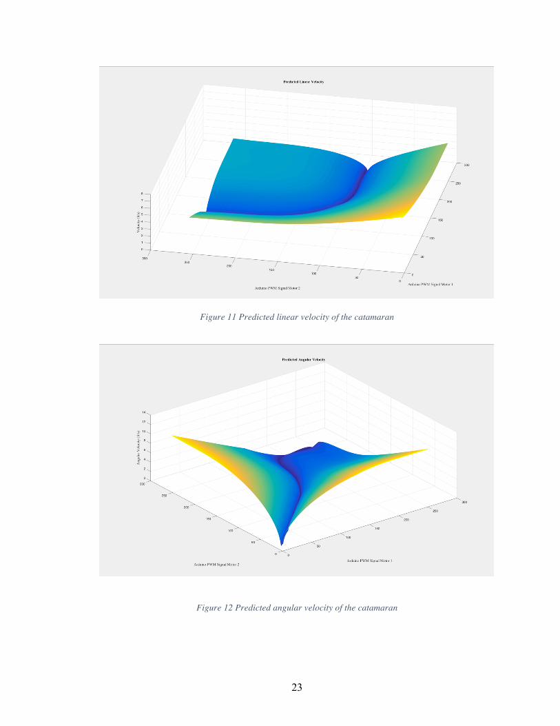
signal inputs. The results can be seen graphically in Figures 13 and 14 below.

23

Figure 11 Predicted linear velocity of the catamaran

Figure 12 Predicted angular velocity of the catamaran

24

Each of the resulting graphs has three axes. The PWM signals for each of the motors are

displayed in two of them, and the linear or angular velocity resulting from the pair is the

third axis.

The linear velocity graph is Figure 13. PWM signals of zero to both motors

produces a peak velocity represented by the yellow portion of the graph. This represents

forward motion. PWM signals of 255 to both motors produces another region of high

velocity. This represents reverse motion. The low region on the graph is the area where

the motors are working against each other and forward and reverse thrust are matched.

The angular velocity graph (Figure 14) is slightly less intuitive. On either side is

a region of intense yellow, this is high velocity. It represents a situation when one motor

is producing forward thrust and the other is producing negative thrust. The low region on

the graph is the area where the motion is completely linear, so the thrust of the motors is

equal. There is a pronounced curve in this region which is present because the thrust

curves of the engines are not identical.

Conclusions and Future Work

The objective of this thesis was to create a dynamic model, and that objective was

met. A system of equations was derived to predict the motion of the 2016 Autonomous

Boat Team’s catamaran, and the drag coefficient and thrust force were determined so the

model could be used.

The equations of motion are 𝑚𝑎 = !!∙ 𝜌 ∙ 𝑥!𝐶!"𝐴 + 2𝐹 and 𝐼𝛼 = !

!"∙ 𝜌 ∙

𝜃!𝐶!"𝐴 + 𝐹! ∙!!− 𝐹! ∙

!!. The combined drag and area coefficient was found, and the

25

drag forces calculated using it were found to have 10.6% error from the measured values.

Thrust curves were generated, and they convey the inability of the engines to produce

negative thrust. This means that the boat cannot travel backwards and cannot turn

effectively with the current propeller design.

The results of this thesis clearly show opportunities for future work on both the

model and the autonomous catamaran. The next step for the catamaran is to add two

more motors mounted in the opposite direction of the first two. With four motors, the

catamaran would be nimbler. The thrust curves for the two additional motors should then

be generated, and the two extra forces should be added to the model.

Though there are many improvements left to be made on this model, I do not want to

understate its merits or undervalue the results that have been produced for the completion

of this project. The thrust curves allowed for the thrust of the motors to be matched,

which is crucial for in making the boat travel forward. The drag curve will be of

significant use for sizing new motors, and with a few modifications to include a third axis

as well as wave and current, hopefully the entire model will prove useful to help the 2017

Autonomous Boat Team make a seaworthy prototype.

26

Bibliography

1. Hydroelectric Power: Managing Water In The West. 1st ed. 2005. Web. 8 Feb. 2016.

2. "Circulation » Gulf Of Maine Census". Gulfofmaine-census.org. N.p., 2016. Web. 13 Mar. 2016.

3. "Cobscook Bay: An Extraordinary Estuary With “Boiling Tides” :: NOAA

Fisheries". Greateratlantic.fisheries.noaa.gov. N.p., 2016. Web. 14 Mar. 2016.

4. Newton, Isaac, William Thomson Kelvin, and Hugh Blackburn. Sir Isaac

Newton's Principia. Glasgow: J. Maclehose, 1871. Print.

5. Ross, Andrew. "A Rudimentary History Of Dynamics". MIC 30.4 (2009): 223-

235. Web.

6. Williams, James H. Fundamentals Of Applied Dynamics. New York: J. Wiley,

1996. Print.

7. Munson, Bruce Roy, Donald F Young, and T. H Okiishi. Fundamentals Of Fluid

Mechanics. New York: Wiley, 1994. Print.

27

APPENDIX A Table 3 Measured velocity and measured and calculated drag

Velocity (ft/sec)

Calculated drag (lbf)

Measured Drag (lbf)

Measured-Calculated Error

2.053 2.688 3.5 0.811 0.231 2.786 4.951 6 1.048 0.174

3.52 7.901 9 1.098 0.122 3.96 10 11.5 1.5 0.130

6.16 24.197 23 -1.197 0.052 6.453 26.556 27 0.443 0.016

7.92 40 40.5 0.5 0.012 TOTAL 0.105

28

APPENDIX B

29

APPENDIX C

Table 4 Raw and processed data collected during experiment

Motor 1 Motor 2 PWM Signal

Raw Force (lbf) Thrust (lbf) Raw Force

(lbf) Thrust (lbf)

255 8 3.0 8.3 3.1 250 7.8 2.9 8.2 3.1 240 7.5 2.8 8.2 3.1 230 7.3 2.7 8.2 3.1 220 7 2.6 8 3.0 210 6.7 2.5 7.8 2.9 200 6.6 2.5 7.8 2.9 190 6.4 2.4 7.7 2.9 180 6.2 2.3 7.6 2.9 100 5.6 2.1 6.9 2.6 90 8.6 3.2 8.6 3.2 80 14.1 5.3 12.5 4.7 70 17.2 6.5 17.3 6.5 60 23.2 8.7 21.3 8.0 50 25.6 9.6 26.1 9.8 40 34 12.8 31.9 12.0 30 39 14.6 38 14.3 20 44 16.5 42 15.8 10 48 18.0 47 17.6 5 50 18.8 46.1 17.3 1 55 20.6 54 20.3

30

APPENDIX D %********************************************************************** %********************************************************************** %*************** Dynamic Model of a Catamaran **************** %*************** By Tamara Thomson **************** %*************** Revised May 5, 2016 **************** %********************************************************************** %********************************************************************** clc, clear all, close all rho=65.55; CdA=.01946; step = 1; b=8.5 for PWM1=1:255/step; for PWM2=1:255/step; if (PWM1<=128/step); F1 = 6.639e-4*(PWM1-128)^2-7.715e-2*(PWM1-128); end if(PWM1 > 128/step) F1 = -1*(3.267e-6*(PWM1-128)^3-8.498e-4*(PWM1-128)^2+7.905e-2*(PWM1-128)); end if (PWM2 <= 128/step); F2 = 6.174e-4*(PWM2-128)^2-7.651e-2*(PWM2-128); end if(PWM2 > 128/step) F2 = -1*(4.791e-6*(PWM2-128)^3-1.259e-3*(PWM2-128)^2+1.076e-1*(PWM2-128)) end V(PWM1,PWM2) = (abs(F1+F2)/(.5*rho*CdA)).^(1/2); %no acceleration w(PWM1,PWM2) = (abs(-F2*b/2+F1*b/2)/(b/16*rho*CdA)).^(1/2); %no acceleration end end V figure hSurf = surf(V,'EdgeColor','none','LineStyle','none','FaceLighting','phong'); figure hSurf = surf(w,'EdgeColor','none','LineStyle','none','FaceLighting','phong');

31

Author’s Biography Tamara R. Thomson was born in Harlingen, Texas on December 12, 1993. She attended

Woodland High School in Baileyville, Maine where she graduated at the top of her class

in 2012. Tamara will graduate from the University of Maine in May of 2016 with a

degree in mechanical engineering and a minor in mathematics. She is a member of Pi

Tau Sigma Honor Society and chapter Vice President of the Society of Women

Engineers.

After graduation, Tamara plans to backpack the Camino de Santiago before beginning a

career with General Motors in July of 2016. Within the first few years of beginning

work, she plans to pursue an advanced degree in engineering.