Dynamic Modeling and Simulation of an Autonomous ...

Dynamic Modeling and Simulation of an Autonomous

Underwater Vehicle (AUV)

A Thesis

SUBMITTED TO THE FACULTY OF THE

UNIVERSITY OF MINNESOTA

BY

Kevin Orpen

IN PARTIAL FULFILLMENT OF THE REQUIREMENTS

FOR THE DEGREE OF

Bachelor of Aerospace Engineering and Mechanics

With Honors

Faculty Adviser: Professor Junaed Sattar, PhD

May 2021

Copyright Page

Copyright © 2021 by Kevin Orpen

i

Acknowledgements

This thesis, and my overall experience with the world of underwater robotics, would not

have been possible without my adviser, Professor Junaed Sattar. I want to thank you for

welcoming me into the Interactive Robotics and Vision Laboratory with open arms. You

have always been such a strong advocate of mine and supported my learning throughout

these past years, and for that, I will forever be grateful.

I would also like to thank Professors Maziar Hemati and Yohannes Ketema for serving on

my thesis committee. Your support and dedication to my research has greatly helped me

refine my work and make this final product a reality.

ii

Abstract

Autonomous Underwater Vehicles (AUVs) have been in development in recent decades to

address the difficulties and high costs of oceanic exploration, with applications including

marine life monitoring, search and rescue operations, and wreck inspection. An underwater

robot developed by the Interactive Robotics and Vision (IRV) Laboratory at the University

of Minnesota is LoCO, a Low Cost Open-Source AUV. LoCO seeks to assist in a number

of underwater applications while reducing the current high cost of entry into underwater

robotics. One aspect of this underwater vehicle that is integral to its capacity as an AUV is

the modeling of its dynamics, and each new AUV comes with unique geometries spanning

various propulsion control methods for specializing in different underwater tasks. This

thesis seeks to establish an underwater dynamic model for the robot, implement the model

in a simulated setting so as to provide testing opportunities before field deployment, and

compare the effectivity of the model to collected experimental data. This, in turn, will lead

to the efficient development of its autonomous systems and capability to assist in

underwater operations. Within this research, the dynamic models have been produced and

geometry-dependent coefficients have been derived for LoCO. A simulator for the robot

has also been developed that can interface with onboard software. Though the simulation

agrees relatively well with experimental data collected for LoCO’s forward motion, there

are still other motion modes that require further investigation. Overall, this dynamic

foundation will provide for future control system and other autonomous development to

further its underwater capabilities.

iii

Table of Contents

List of Tables ..................................................................................................................... vi

List of Figures ................................................................................................................... vii

Chapter 1 Introduction ................................................................................................... 1

1.1. Background .......................................................................................................... 1

1.2. LoCO Design........................................................................................................ 2

1.3. Thesis Objective ................................................................................................... 3

1.4. Overview .............................................................................................................. 4

Chapter 2 Derivation of Dynamic Equations ................................................................ 5

2.1. Introduction .......................................................................................................... 5

2.2. Body Frame Definition......................................................................................... 5

2.3. Relationship Between Inertial and Body Coordinate Frames .............................. 8

2.4. Rigid Body 6-Degrees of Freedom Equations of Motion .................................. 10

2.5. Forces and Moments .......................................................................................... 12

2.5.1. Environmental Forces ................................................................................. 12

2.5.2. Propulsion ................................................................................................... 13

2.5.3. Restoring Forces ......................................................................................... 14

2.5.4. Added Mass ................................................................................................ 14

iv

2.5.5. Hydrodynamic Damping ............................................................................. 17

2.6. Overall Kinetics Equations................................................................................. 19

2.7. Conclusion .......................................................................................................... 20

Chapter 3 Estimation of LoCO Dynamic Parameters ................................................. 21

3.1. Introduction ........................................................................................................ 21

3.2. Buoyancy ............................................................................................................ 21

3.3. Mass and Moments of Inertia ............................................................................. 23

3.4. Added Mass Coefficients ................................................................................... 26

3.5. Hydrodynamic Damping Coefficients ............................................................... 36

3.6. Dynamic Equations for LoCO............................................................................ 42

3.7. Conclusion .......................................................................................................... 44

Chapter 4 Simulation ................................................................................................... 46

4.1. Introduction ........................................................................................................ 46

4.2. Modeling and Visualization ............................................................................... 46

4.3. Physics ................................................................................................................ 48

4.4. Simulation Architecture and Control ................................................................. 49

4.5. Quaternions and Force Application.................................................................... 50

4.6. Conclusion .......................................................................................................... 51

Chapter 5 Experimental Data and Comparison with Simulation ................................ 53

v

5.1. Introduction ........................................................................................................ 53

5.2. Experiment and Data Analysis ........................................................................... 53

5.3. Simulation Data Comparison ............................................................................. 55

5.4. Conclusion .......................................................................................................... 57

Chapter 6 Conclusion .................................................................................................. 58

6.1. Review ................................................................................................................ 58

6.2. Conclusions ........................................................................................................ 58

6.3. Future Work ....................................................................................................... 59

References ......................................................................................................................... 60

Appendix A ....................................................................................................................... 63

vi

List of Tables

Table 1: Vehicle buoyancy analysis summary................................................................. 22

Table 2: Vehicle mass and moments of inertia analysis summary. ................................. 25

Table 3: Table of components and corresponding variable names for geometric LoCO

models. .............................................................................................................................. 29

Table 4: Added mass analysis values. .............................................................................. 36

Table 5: Summary of component coefficients of drag..................................................... 38

Table 6: Summary of component drag reference areas. .................................................. 38

Table 7: Summary of hydrodynamic damping analysis results. ...................................... 42

Table 8: Relevant dynamic model parameters from analysis and estimation. ................. 43

Table 9: LoCO Component Matrix for mass and moment of inertia determination. ...... 64

vii

List of Figures

Figure 1: LoCO in untethered deployment in the Caribbean Sea near Barbados [4]. ....... 2

Figure 2: LoCO CAD model in SolidWorks. .................................................................... 2

Figure 3: LoCO body-fixed coordinate frame definition overall view. ............................. 6

Figure 4: LoCO body-fixed coordinate frame definition section views. ........................... 7

Figure 5: Relationship between body frame and inertial frame. ........................................ 8

Figure 6: Example of notation for rectangular prism of square cross section rotating

about one end (rotation about the dashed line). ................................................................ 18

Figure 7: Moments of inertia for hollow cylinder and rectangular prism [20]. ............... 24

Figure 8: Parallel axis theorem example, where m is mass of the object. ....................... 25

Figure 9: Geometric approximation for LoCO flow in x-direction – “X-Model”. .......... 28

Figure 10: Geometric approximation for LoCO flow in y-direction – “Y-Model”. ........ 28

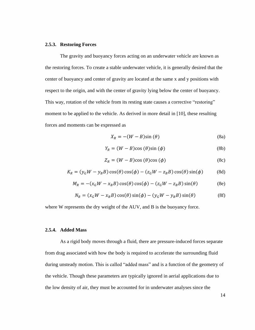
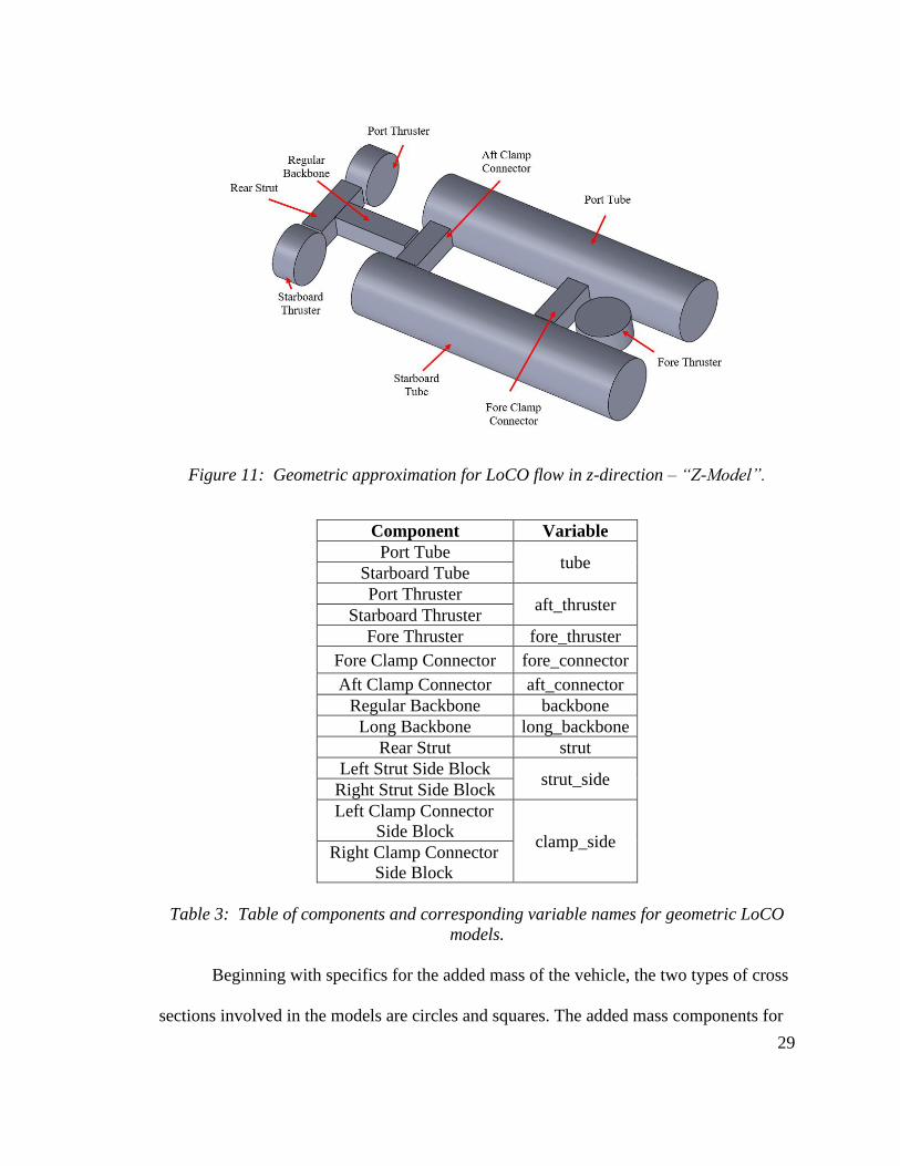
Figure 11: Geometric approximation for LoCO flow in z-direction – “Z-Model”.......... 29

Figure 12: Added mass parameters for a circle and a square [13], [21]. ......................... 30

Figure 13: LoCO in a simulated Gazebo world. .............................................................. 47

Figure 14: ROS program nodes and messages used to run the simulation. ..................... 50

Figure 15: Thruster force versus PWM input [28]........................................................... 54

Figure 16: Velocity versus forward thrust applied for a straight line, horizontal path in a

pool. .................................................................................................................................. 55

Figure 17: Velocity versus full forward thrust applied for a straight line, horizontal path.

........................................................................................................................................... 56

viii

Figure 18: Clockwise penetrator numbering convention. ................................................ 64

1

Chapter 1

Introduction

1.1. Background

Ocean exploration began in the late 19th century with the search for a greater

understanding of how the Earth works and the life it holds. Since then, discoveries across

the span of 71% of the Earth’s surface have yielded entirely new fields of study and

revolutionary findings in areas such as geology, marine biology, and environmental

science. However, the majority of Earth’s oceans remain unexplored, due in part to high

resource and economic costs [1]. This, along with the quest to explore deep sea areas

extremely difficult for humans to reach, has spurred the field of underwater robotics.

Autonomous Underwater Vehicles (AUVs) have been in development in recent decades

to address the high cost of underwater exploration. Other applications of these

technologies include marine life monitoring, mineral exploration, global environment

evaluation, wreck inspection, and search and rescue operations. The dynamic underwater

environment comes with a host of new challenges though, ranging from navigation where

GPS does not function to environments of operation prone to unpredictable disturbances

[2]. An example of underwater robotics development for oceanography research can be

found with the Seaglider [3], where the AUV is designed to operate for long periods of

time to gather ocean data at a fraction of the cost of manned expeditions. Though

research in underwater robotics has greatly progressed, the sensors and equipment

required for accurate navigation and reliable operation in underwater environments often

come at high costs.

2

1.2. LoCO Design

An AUV developed by the Interactive Robotics and Vision (IRV) Laboratory at

the University of Minnesota is LoCO. LoCO AUV is a Low-Cost, Open-Source,

Autonomous Underwater Vehicle. It is vision-guided and rated to a depth of 100 meters,

capable of being deployed by a single person in the field [4]. A picture of LoCO in an

ocean deployment can be seen below, along with the corresponding Computer Aided

Design (CAD) model in SolidWorks. This underwater vehicle seeks to assist personnel in

numerous underwater applications in a more cost-effective manner than previous robots.

Figure 1: LoCO in untethered deployment in the Caribbean Sea near Barbados [4].

Figure 2: LoCO CAD model in SolidWorks.

3

One aspect of LoCO that is integral to its capacity as an AUV is the modeling of

its dynamics. For a reliable control system to be developed that enables autonomous

operation, a foundation in the dynamics of the robot must be established. Though a

number of studies have been conducted on the modeling of AUVs in an underwater

environment [5], [6], and the governing equations for marine hydrodynamics have been

established, each new AUV comes with unique geometries. Further, AUV designs boast

various propulsion control methods for the underwater tasks they are primarily designed

for.

1.3. Thesis Objective

This thesis seeks to evaluate the known properties common to any underwater

environment and apply foundational components to characterize the underwater

dynamics of the LoCO AUV. Work is performed to implement these dynamics in a

simulated environment, able to be integrated with onboard robot systems, in order to

provide a mode of testing software before resource-costly field trials. Experimental

testing data is compared to the simulation implementation of the dynamic model. These

outcomes, in turn, will lead to the efficient development of future control systems to

assist in underwater research including trash detection development, vision system

development, and human-robot interaction research [7].

4

1.4. Overview

The content discussed herein serves to first provide a foundation in the governing

dynamics and various definitions for LoCO in Chapter 2. A number of assumptions are

previewed before a brief description of the relation between dynamics derived in the

frame of a rigid body and the corresponding motion in an inertial frame. The general

dynamic equations for a 6-Degrees-of-Freedom (DoF) body are derived and associated

forces for the underwater robot are discussed. Chapter 3 takes these general equations and

describes the various estimation methods used to evaluate the coefficient parameters in

the dynamic equations specific to the vehicle. A final list of estimated parameters is

presented along with the resulting simplified dynamic equations. Chapter 4 discusses the

simulation component of the thesis, including its program architecture and application of

forces. Chapter 5 looks at how the simulation is utilized to compare the dynamic model to

experimental data collected. Finally, Chapter 6 summarizes the thesis in conclusion of the

work.

5

Chapter 2

Derivation of Dynamic Equations

2.1. Introduction

Before any specific dynamic estimates regarding LoCO can be made, the dynamic

framework and general equations of motion must be derived. Though these derivations

can be found in a number of texts [8]–[10], they are included within this thesis so that the

document may be self-sufficient. Governing assumptions that are being made for this

dynamic model will be explained in each of the appropriate sections, but are listed below

as an overview [8]:

1) The AUV can be treated as a rigid body of a constant mass.

2) The earth’s rotation is negligible for acceleration components of the vehicle’s

center of mass.

3) The thrusters are assumed to be a constant source of thrust.

4) The underwater vehicle is sufficiently submerged in an unbounded and ideal fluid.

5) The AUV does not experience underwater currents.

6) The AUV is assumed to not be a streamlined body due to external irregularities

such as clamps.

2.2. Body Frame Definition

There are often two frames of reference used in expressing the equations of

motion for an underwater vehicle. One of these is a “body” coordinate frame, which is

fixed to the body of the marine vehicle. It is beneficial in many other applications to

6

attach the origin of the coordinate system to the center of gravity of the vehicle.

However, especially with a vehicle that can be modified such as LoCO, the center of

gravity may change throughout the design cycle of the vehicle. Along with modeling

benefits explained later regarding body-fixed origin placement along lines of symmetry,

it is common to define the body-fixed coordinate frame origin at a location other than the

center of gravity. The coordinate system for LoCO can be seen below in Fig. 3. In marine

engineering, velocities in the x, y, and z directions are defined as surge (u), sway (v), and

heave (w), respectively, with overall forces along the axes noted as X, Y, and Z.

Similarly, angular velocities about those same axes are defined as roll (p), pitch (q), and

yaw (r), respectively, with overall moments along the axes noted as K, M, and N.

Figure 3: LoCO body-fixed coordinate frame definition overall view.

7

Figure 4: LoCO body-fixed coordinate frame definition section views.

As can be seen in Figs. 3 and 4, LoCO has geometric planes of symmetry about

the x-z plane and x-y plane. For the case of this analysis, the body frame origin for LoCO

is located at the intersection of these two planes and along the x axis to the back face of

the rear end cap. This way, the characteristics of the robot can change with minimal

effect to the dynamic framework of the thesis. More will be discussed on the force-

related advantages to this origin location as well.

8

2.3. Relationship Between Inertial and Body Coordinate Frames

The second frame used as reference for these equations of motion is an inertial

frame that the underwater vehicle operates in. For this analysis, an Earth-fixed inertial

system will be used called “NED”, or “North-East-Down” [10]. In this case, the x

direction of the coordinate system points North, the y direction points East, and the z

direction therefore points downwards.

Though much of this thesis is devoted to the analysis of motion and forces in the

body-fixed frame defined above, for any mission with an underwater vehicle, it is critical

to relate the state of the vehicle back to the overall frame of reference. A visual depiction

of the relation between the Earth-fixed frame and the body-fixed frame is given below in

Fig. 5. The position of the vehicle in relation to the Earth frame is often given in terms of

XE, YE, and ZE, along their respective axes. The angle of rotation about each of these axes

is denoted as ϕ, θ, and ψ, respectively.

Figure 5: Relationship between body frame and inertial frame.

9

Euler angles give a way of relating the orientation of a rigid body in three-

dimensional space with reference to an original reference frame through three single-axis

rotations. Though there are multiple possible conventions for achieving this, one example

is the Euler “3-2-1”, or “Z-Y-X”, sequence. Each rotation is represented by a 3 x 3

matrix, with the first rotation about the original z-axis by the yaw angle, denoted as

Rz(ψ). Then, a rotation about the following y-axis by the pitch angle is performed, and

finally a rotation about the following x-axis by the roll angle. More detail on these

rotation matrices and Euler angles can be found in various sources such as [11], [12].

Overall, a final relationship between the velocity of the underwater vehicle in Earth frame

coordinates and body frame coordinates can then be represented as

[𝑢𝑣𝑤

] = 𝑅𝑥(𝜙)𝑅𝑦(θ)𝑅𝑧(ψ) [

𝑋�̇�

𝑌�̇�

𝑍�̇�

]

= [

1 0 00 cos (𝜙) sin (𝜙)0 −sin (𝜙) cos (𝜙)

] [cos (𝜃) 0 −sin (𝜃)

0 1 0sin (𝜃) 0 cos (𝜃)

] [cos (𝜓) sin (𝜓) 0−sin (𝜓) cos (𝜓) 0

0 0 1

] [

𝑋�̇�

𝑌�̇�

𝑍�̇�

]

= [

cos (𝜃)cos (𝜓)

− sin(𝜓) cos(𝜙) + sin (𝜙)sin (𝜃)cos (𝜓)

sin(𝜙) sin(𝜓) + cos (𝜙)cos (𝜓)sin (𝜃)…

cos (𝜃)sin (𝜓)

cos(𝜙) cos(𝜓) + sin (𝜙)sin (𝜃)sin (𝜓)

− sin(𝜙) cos(𝜓) + cos (𝜙)sin (𝜃)sin (𝜓)…

−sin (𝜃)sin (𝜙)cos (𝜃)cos (𝜙)cos (𝜃)

] [

𝑋�̇�

𝑌�̇�

𝑍�̇�

] (1)

10

To achieve a similar transformation for angular velocities, each Euler angle

derivative must be addressed separately since they are not independent orthogonal

elements. So,

[𝑝𝑞𝑟] = 𝑅𝑥(ϕ)𝑅𝑦(θ)𝑅𝑧(ψ) [

00�̇�

] + 𝑅𝑥(ϕ)𝑅𝑦(θ) [0�̇�0] + 𝑅𝑥(ϕ) [

�̇�00

]

𝑝 = �̇� − sin (𝜃)�̇� (2a)

𝑞 = sin(𝜙) cos(𝜃) �̇� + 𝑐𝑜𝑠(𝜙)�̇� (2b)

𝑟 = cos (𝜙)cos (𝜃)�̇� − sin(𝜙)�̇� (2c)

One drawback of Euler angle representation of the motion of the vehicle is what is

known as “gimbal lock”, or when there is a singularity in the equations of motion, such as

that caused by a pitch value of 90 degrees. For the sake of expressing the relationships as

most commonly used in marine dynamics, the resulting equations of motion as derived

above hold their value since large pitch angles are usually avoided with submarines or

other streamlined underwater vehicles [9]. An alternate way to express rotations are

quaternions. Though they can be more complicated than expressions with Euler angles,

they eliminate the issue with singularity and provide computationally easier ways to work

with rotations. Quaternions, and how they are implemented in simulation, are discussed

later.

2.4. Rigid Body 6-Degrees of Freedom Equations of Motion

As given in the first two assumptions, the equations of motion for LoCO can be

derived as those for a rigid body with constant mass and six degrees of freedom. The

11

following set of equations applies to a body-fixed coordinate frame in which the center of

gravity is not necessarily the center of the coordinate system, derived within Newton-

Euler framework. This can be seen defined in Figs. 3 and 4 for LoCO, where the forces

and moments of the following derivation are taken about the origin of the body system.

Beginning with an expression of Newton’s second law, the forces on the body are

equivalent to the time derivative of linear momentum. When dealing with rotating

coordinate frames inside an overall inertial frame, rotational effects on changes in

momentum must be compensated for besides linear acceleration. This leads to

𝑭 =𝑑

𝑑𝑡(𝑚𝑼) = 𝑚 (�̇� + 𝝎 × 𝑼 + 𝜶 × 𝒓𝑮 + 𝝎 × (𝝎 × 𝒓𝑮)) (3)

where bold notation indicates vectors, in which U is linear velocity of the vehicle origin,

ω is the angular velocity of the body system, α is the angular acceleration, and rG is the

position vector from the origin of the coordinate frame to the vehicle center of gravity. In

this equation, the first term in the translational acceleration, the second is the Coriolis

term, the third is the azimuthal acceleration, and the final term is the centripetal

acceleration.

Now for the moments on the vehicle, the sum of these is equivalent to the time

derivative of angular momentum. Similar to dealing with a rotating frame in equation 3,

𝑴 =𝑑

𝑑𝑡(𝑰𝝎) = 𝑰 ∙ 𝜶 + 𝝎 × (𝑰 ∙ 𝝎) + 𝑚 ∙ 𝒓𝑮 × (�̇� + 𝝎 × 𝑼) (4)

where the same notation is used from equation 3, and I is the moment of inertia matrix

for the body given with the matrix,

𝑰 = [

𝐼𝑥 −𝐼𝑥𝑦 −𝐼𝑥𝑧

−𝐼𝑦𝑥 𝐼𝑦 −𝐼𝑦𝑧

−𝐼𝑧𝑥 −𝐼𝑧𝑦 𝐼𝑧

] (5)

12

More in-depth derivations of these equations of motion can be found in sources

such as [8]–[10]. Evaluating equation 3 for the axial force, lateral force, and vertical force

equations,

𝑋 = 𝑚(�̇� − 𝑣𝑟 + 𝑤𝑞 − 𝑥𝐺(𝑞2 + 𝑟2) + 𝑦𝐺(𝑝𝑞 − �̇�) + 𝑧𝐺(𝑝𝑟 − �̇�)) (6a)

𝑌 = 𝑚(�̇� − 𝑤𝑝 + 𝑢𝑟 + 𝑥𝐺(𝑞𝑝 + �̇�) − 𝑦𝐺(𝑟2 + 𝑝2) + 𝑧𝐺(𝑞𝑟 − �̇�)) (6b)

𝑍 = 𝑚(�̇� − 𝑢𝑞 + 𝑣𝑝 + 𝑥𝐺(𝑟𝑝 − �̇�) + 𝑦𝐺(𝑟𝑞 + �̇�) − 𝑧𝐺(𝑝2 + 𝑞2)) (6c)

Evaluating equation 4 for the moment about the roll moment, pitch moment, and

yaw moment,

𝐾 = 𝐼𝑥�̇� + (𝐼𝑧 − 𝐼𝑦)𝑞𝑟 − (�̇� + 𝑝𝑞)𝐼𝑥𝑧 + (𝑟2 − 𝑞2)𝐼𝑦𝑧 + (𝑝𝑟 − �̇�)𝐼𝑥𝑦 …

+ 𝑚(𝑦𝐺(�̇� − 𝑢𝑞 + 𝑣𝑝) − 𝑧𝐺(�̇� − 𝑤𝑝 + 𝑢𝑟)) (6d)

𝑀 = 𝐼𝑦�̇� + (𝐼𝑥 − 𝐼𝑧)𝑟𝑝 − (�̇� + 𝑞𝑟)𝐼𝑥𝑦 + (𝑝2 − 𝑟2)𝐼𝑥𝑧 + (𝑞𝑝 − �̇�)𝐼𝑦𝑧 …

+ 𝑚(𝑧𝐺(�̇� − 𝑣𝑟 + 𝑤𝑞) − 𝑥𝐺(�̇� − 𝑢𝑞 + 𝑣𝑝)) (6e)

𝑁 = 𝐼𝑧�̇� + (𝐼𝑦 − 𝐼𝑥)𝑝𝑞 − (�̇� + 𝑟𝑝)𝐼𝑦𝑧 + (𝑞2 − 𝑝2)𝐼𝑥𝑦 + (𝑟𝑞 − �̇�)𝐼𝑥𝑧 …

+ 𝑚(𝑥𝐺(�̇� − 𝑤𝑝 + 𝑢𝑟) − 𝑦𝐺(�̇� − 𝑣𝑟 + 𝑤𝑞)) (6f)

2.5. Forces and Moments

2.5.1. Environmental Forces

One of the primary assumptions for this dynamic analysis lies with the

environmental forces. In a full seakeeping analysis of an underwater vehicle, surface

effects, radiation-induced damping, and other wave effects are taken into account. These

variables can come to be very dependent upon the situation involved for the vehicle.

Since LoCO is designed to operate in a range of environments, these wave-dependent

13

effects and surface effects are ignored with the assumption that the AUV is sufficiently

submerged underwater.

2.5.2. Propulsion

The propulsion for LoCO is governed with three thrusters. The rear port and

starboard thrusters control movement in the horizontal plane, while the vertical thruster

adds control in the vertical plane. Each thruster is referred to as “port”, “stbd”, and

“fore”, respectively. One assumption regarding the analysis with the thrusters is that they

act as point forces at the center of the thruster propellers. Though the actual thrusters

have inherent propeller dynamics, the point force simplification has been made for this

analysis as a reasonable approximation. As for the reaction torques of each thruster, the

port and starboard thrusters have propellers that provide the same forward thrust while

spinning in opposite directions, so the moments cancel each other. It also assumed that

the moment produced by the force thruster is negligible with respect to the larger vehicle

dynamics and is ignored. With this, the forces and moments created by the thrusters can

be expressed with the same conventions as established in section 2.4.

𝑋𝑃 = 𝑇𝑝𝑜𝑟𝑡 + 𝑇𝑠𝑡𝑏𝑑 (7a)

𝑌𝑃 = 0 (7b)

𝑍𝑃 = 𝑇𝑓𝑜𝑟𝑒 (7c)

𝐾𝑃 = 0 (7d)

𝑀𝑃 = −𝑇𝑓𝑜𝑟𝑒 𝑥𝑓𝑜𝑟𝑒 (7e)

𝑁𝑃 = −𝑇𝑝𝑜𝑟𝑡 𝑦𝑝𝑜𝑟𝑡 − 𝑇𝑠𝑡𝑏𝑑 𝑦𝑠𝑡𝑏𝑑 (7f)

14

2.5.3. Restoring Forces

The gravity and buoyancy forces acting on an underwater vehicle are known as

the restoring forces. To create a stable underwater vehicle, it is generally desired that the

center of buoyancy and center of gravity are located at the same x and y positions with

respect to the origin, and with the center of gravity lying below the center of buoyancy.

This way, rotation of the vehicle from its resting state causes a corrective “restoring”

moment to be applied to the vehicle. As derived in more detail in [10], these resulting

forces and moments can be expressed as

𝑋𝑅 = −(𝑊 − 𝐵)sin (𝜃) (8a)

𝑌𝑅 = (𝑊 − 𝐵)cos (𝜃)sin (𝜙) (8b)

𝑍𝑅 = (𝑊 − 𝐵)cos (𝜃)cos (𝜙) (8c)

𝐾𝑅 = (𝑦𝐺𝑊 − 𝑦𝐵𝐵) cos(𝜃) cos(𝜙) − (𝑧𝐺𝑊 − 𝑧𝐵𝐵) cos(𝜃) sin(𝜙) (8d)

𝑀𝑅 = −(𝑥𝐺𝑊 − 𝑥𝐵𝐵) cos(𝜃) cos(𝜙) − (𝑧𝐺𝑊 − 𝑧𝐵𝐵) sin(𝜃) (8e)

𝑁𝑅 = (𝑥𝐺𝑊 − 𝑥𝐵𝐵) cos(𝜃) sin(𝜙) − (𝑦𝐺𝑊 − 𝑦𝐵𝐵) sin(𝜃) (8f)

where W represents the dry weight of the AUV, and B is the buoyancy force.

2.5.4. Added Mass

As a rigid body moves through a fluid, there are pressure-induced forces separate

from drag associated with how the body is required to accelerate the surrounding fluid

during unsteady motion. This is called “added mass” and is a function of the geometry of

the vehicle. Though these parameters are typically ignored in aerial applications due to

the low density of air, they must be accounted for in underwater analyses since the

15

density of the fluid is much higher and on the same order as that of the rigid body. The

forces and moments are expressed as described in [13]

𝐹𝑗 = −�̇�𝑖𝑚𝑖𝑗 − 𝜀𝑗𝑘𝑙𝑈𝑖𝜔𝑘𝑚𝑙𝑖 (9a)

𝑀𝑗 = −�̇�𝑖𝑚𝑗+3,𝑖 − 𝜀𝑗𝑘𝑙𝑈𝑖𝜔𝑘𝑚𝑙+3,𝑖 − 𝜀𝑗𝑘𝑙𝑈𝑘𝑈𝑖𝑚𝑙𝑖 (9b)

where j denotes the direction of the force, i=1, 2, 3, 4, 5, 6 and j, k, l = 1, 2, 3. εjkl is the

alternating tensor where

𝜀𝑗𝑘𝑙 = {

0; if any pair of the indices j, k, l are equal1; if j, k, l are in cyclic order−1; if j, k, l are in anti − cyclic order

(10)

The overall effect of this added mass is more commonly condensed into an

symmetrical added mass or inertia matrix using Society of Naval Architects and Marine

Engineers (SNAME) notation [14] as

𝑀𝐴 =

[ 𝑋�̇� 𝑋�̇� 𝑋�̇�

𝑌�̇� 𝑌�̇� 𝑌�̇�

𝑍�̇� 𝑍�̇� 𝑍�̇�

𝑋�̇� 𝑋�̇� 𝑋�̇�

𝑌�̇� 𝑌�̇� 𝑌�̇�

𝑍�̇� 𝑍�̇� 𝑍�̇�

𝐾�̇� 𝐾�̇� 𝐾�̇�

𝑀�̇� 𝑀�̇� 𝑀�̇�

𝑁�̇� 𝑁�̇� 𝑁�̇�

𝐾�̇� 𝐾�̇� 𝐾�̇�

𝑀�̇� 𝑀�̇� 𝑀�̇�

𝑁�̇� 𝑁�̇� 𝑁�̇� ]

(11)

Overall, the expanded equations for forces and moments on the rigid body due to

the added mass terms can be expressed as derived by Imlay [15],

𝑋𝐴 = 𝑋�̇��̇� + 𝑋�̇�(�̇� + 𝑢𝑞) + 𝑋�̇��̇� + 𝑍�̇�𝑤𝑞 + 𝑍�̇�𝑞2

+𝑋�̇��̇� + 𝑋�̇��̇� + 𝑋�̇��̇� − 𝑌�̇�𝑣𝑟 − 𝑌�̇�𝑟𝑝 − 𝑌�̇�𝑟2

−𝑋�̇�𝑢𝑟 − 𝑌�̇�𝑤𝑟

+𝑌�̇�𝑣𝑞 + 𝑍�̇�𝑝𝑞 − (𝑌�̇� − 𝑍�̇�)𝑞𝑟 (12a)

16

𝑌𝐴 = 𝑋�̇��̇� + 𝑌�̇��̇� + 𝑌�̇��̇�

+𝑌�̇��̇� + 𝑌�̇��̇� + 𝑌�̇��̇� + 𝑋�̇�𝑣𝑟 − 𝑌�̇�𝑣𝑝 + 𝑋�̇�𝑟2 + (𝑋�̇� − 𝑍�̇�)𝑟𝑝 − 𝑍�̇�𝑝2

−𝑋�̇�(𝑢𝑝 − 𝑤𝑟) + 𝑋�̇�𝑢𝑟 − 𝑍�̇�𝑤𝑝

−𝑍�̇�𝑝𝑞 + 𝑋�̇�𝑞𝑟 (12b)

𝑍𝐴 = 𝑋�̇�(�̇� − 𝑤𝑞) + 𝑍�̇��̇� + 𝑍�̇��̇� − 𝑋�̇�𝑢𝑞 − 𝑋�̇�𝑞2

+𝑌�̇��̇� + 𝑍�̇��̇� + 𝑍�̇��̇� + 𝑌�̇�𝑣𝑝 + 𝑌�̇�𝑟𝑝 + 𝑌�̇�𝑝2

+𝑋�̇�𝑢𝑝 + 𝑌�̇�𝑤𝑝

−𝑋�̇�𝑣𝑞 − (𝑋�̇� − 𝑌�̇�)𝑝𝑞 − 𝑋�̇�𝑞𝑟 (12c)

𝐾𝐴 = 𝑋�̇��̇� + 𝑍�̇��̇� + 𝐾�̇��̇� − 𝑋�̇�𝑤𝑢 + 𝑋�̇�𝑢𝑞 − 𝑌�̇�𝑤2 − (𝑌�̇� − 𝑍�̇�)𝑤𝑞 + 𝑀�̇�𝑞2

+𝑌�̇��̇� + 𝐾�̇��̇� + 𝐾�̇��̇� + 𝑌�̇�𝑣2 − (𝑌�̇� − 𝑍�̇�)𝑣𝑟 + 𝑍�̇�𝑣𝑝 − 𝑀�̇�𝑟2 − 𝐾�̇�𝑟𝑝

+𝑋�̇�𝑢𝑣 − (𝑌�̇� − 𝑍�̇�)𝑣𝑤 − (𝑌�̇� + 𝑍�̇�)𝑤𝑟 − 𝑌�̇�𝑤𝑝 − 𝑋�̇�𝑢𝑟

+(𝑌�̇� + 𝑍�̇�)𝑣𝑞 + 𝐾�̇�𝑝𝑞 − (𝑀�̇� − 𝑁�̇�)𝑞𝑟 (12d)

𝑀𝐴 = 𝑋�̇�(�̇� + 𝑤𝑞) + 𝑍�̇�(�̇� − 𝑢𝑞) + 𝑀�̇��̇� − 𝑋�̇�(𝑢2 − 𝑤2) − (𝑍�̇� − 𝑋�̇�)𝑤𝑢

+𝑌�̇��̇� + 𝐾�̇��̇� + 𝑀�̇��̇� + 𝑌�̇�𝑣𝑟 − 𝑌�̇�𝑣𝑝 − 𝐾�̇�(𝑝2 − 𝑟2) + (𝐾�̇� − 𝑁�̇�)𝑟𝑝

−𝑌�̇�𝑢𝑣 + 𝑋�̇�𝑣𝑤 − (𝑋�̇� + 𝑍�̇�)(𝑢𝑝 − 𝑤𝑟) + (𝑋�̇� − 𝑍�̇�)(𝑤𝑝 + 𝑢𝑟)

−𝑀�̇�𝑝𝑞 + 𝐾�̇�𝑞𝑟 (12e)

𝑁𝐴 = 𝑋�̇��̇� + 𝑍�̇��̇� + 𝑀�̇��̇� + 𝑋�̇�𝑢2 + 𝑌�̇�𝑤𝑢 − (𝑋�̇� − 𝑌�̇�)𝑢𝑞 − 𝑍�̇�𝑤𝑞 − 𝐾�̇�𝑞

2

+𝑌�̇��̇� + 𝐾�̇��̇� + 𝑁�̇��̇� − 𝑋�̇�𝑣2 − 𝑋�̇�𝑣𝑟 − (𝑋�̇� − 𝑌�̇�)𝑣𝑝 + 𝑀�̇�𝑟𝑝 + 𝐾�̇�𝑝

2

−(𝑋�̇� − 𝑌�̇�)𝑢𝑣 − 𝑋�̇�𝑣𝑤 + (𝑋�̇� + 𝑌�̇�)𝑢𝑝 + 𝑌�̇�𝑢𝑟 + 𝑍�̇�𝑤𝑝

−(𝑋�̇� + 𝑌�̇�)𝑣𝑞 − (𝐾�̇� − 𝑀�̇�)𝑝𝑞 − 𝐾�̇�𝑞𝑟 (12f)

17

The equations were formatted by Imlay [15] so that the longitudinal components

are on the first line, lateral components are on the second line, mixed terms involving u or

w are on the third line, and mixed second order terms that are sometimes neglected are

placed on the fourth line.

2.5.5. Hydrodynamic Damping

The final set of forces being considered in this analysis is the hydrodynamic

damping forces. The main damping force is the viscous damping force due to vortex

shedding, given by the general equation

𝐹𝐷 = −1

2𝜌𝐶𝐷(𝑅𝑛)𝐴|𝑢|𝑢 (13)

where ρ is the fluid density, CD is the coefficient of drag that is dependent upon the

Reynolds number, Rn, A is the corresponding reference area to the applied coefficient of

drag, and u is the velocity of the vehicle. The equation for the Reynolds number of a

given geometry is

𝑅𝑛 =𝑢𝐷

𝜈 (14)

where D is the characteristic length of the geometry and 𝜈 (“nu”, not “v”) is the kinematic

viscosity for the surrounding fluid [16].

The drag on a body rotating in a fluid can be related to the linear damping using

the following equation

𝜔 ∙ 𝑟 = 𝑢 (15)

where ω is the instantaneous angular velocity of the rotating body, and r is the distance

from the axis of rotation to a specific cross section of the body. In this case, the

18

corresponding linear force would be multiplied by that same distance from the axis of

rotation to obtain the moment. This moment arm must be integrated due to the face that

each successive cross section of a body with a given damping coefficient may lie a

different distance away from the axis of rotation.

Overall, the drag moment can be approximated as

𝑀𝐷 = ∫(𝐹𝐷 ⊥ 𝑟) = −1

2𝜌𝐶𝐷(𝑅𝑛) ∫ (𝑏 ∙ 𝑑𝑟) ∙ |𝜔 ∙ 𝑟| ∙ (𝜔 ∙ 𝑟)

𝑟2

𝑟1∙ 𝑟

= −1

2𝜌𝐶𝐷(𝑅𝑛)𝑏|𝜔|𝜔 ∙ ∫ 𝑟2|𝑟|𝑑𝑟

𝑟2

𝑟1 (16)

where the variable “b” is introduced to represent the reference area length of each

successive cross section that is parallel to the axis of rotation. An example of this is given

in the diagram below in Fig. 6 for a rectangular prism of square cross section being

rotated about its end. It should be noted that some of the general dynamics nomenclature

when addressing damping equations overlaps with that addressing the other marine

dynamics nomenclature, such as “r”. The notation with hydrodynamic damping can be

considered isolated from other nomenclature unless specifically noted in the text.

Figure 6: Example of notation for rectangular prism of square cross section rotating

about one end (rotation about the dashed line).

Where the damping due to vortex shedding, or pressure drag, often uses the

reference area of the body perpendicular to the flow, nonlinear skin friction across the

19

surface area of the vehicle is also taken into account. This is notated with a skin friction

coefficient of drag using equation 13, with CF instead of CD. There can also be lift forces

associated with vortex shedding, especially with streamlined bodies or ones generally

shaped as airfoils [16]. With the many irregularities on LoCO’s surface, it is generally not

being considered a streamlined body and it is assumed that any lift forces generated by

the vehicle are negligible in comparison to drag forces.

The non-velocity terms are typically condensed into a single coefficient, with the

subscript indicating the direction of motion causing the force. Also due to asymmetry,

there will be a net pitching moment generated by linear movement in the vertical

direction, and a net yawing moment generated by linear movement in the lateral

direction. Overall, the expanded equations for forces and moments on the rigid body due

to the hydrodynamic damping terms [17] can be expressed as

𝑋𝐷 = 𝑋𝑢|𝑢|𝑢|𝑢| (17a)

𝑌𝐷 = 𝑌𝑣|𝑣|𝑣|𝑣| (17b)

𝑍𝐷 = 𝑍𝑤|𝑤|𝑤|𝑤| (17c)

𝐾𝐷 = 𝐾𝑝|𝑝|𝑝|𝑝| (17d)

𝑀𝐷 = 𝑀𝑞|𝑞|𝑞|𝑞|+𝑀𝑤|𝑤|𝑤|𝑤| (17e)

𝑁𝐷 = 𝑁𝑟|𝑟|𝑟|𝑟|+𝑁𝑣|𝑣|𝑣|𝑣| (17f)

2.6. Overall Kinetics Equations

Tying together each of the force and moment components acting on the AUV,

𝑋 = 𝑋𝑃 + 𝑋𝑅 + 𝑋𝐷 − 𝑋𝐴 (18a)

20

𝑌 = 𝑌𝑃 + 𝑌𝑅 + 𝑌𝐷 − 𝑌𝐴 (18b)

𝑍 = 𝑍𝑃 + 𝑍𝑅 + 𝑍𝐷 − 𝑍𝐴 (18c)

𝐾 = 𝐾𝑃 + 𝐾𝑅 + 𝐾𝐷 − 𝐾𝐴 (18d)

𝑀 = 𝑀𝑃 + 𝑀𝑅 + 𝑀𝐷 − 𝑀𝐴 (18e)

𝑁 = 𝑁𝑃 + 𝑁𝑅 + 𝑁𝐷 − 𝑁𝐴 (18f)

2.7. Conclusion

In this chapter, a body-fixed reference frame is defined for the underwater vehicle

and parameters for motion along these body axes are related back to the overall inertial

frame. The 6-degrees-of-freedom equations of motion for such a rigid body are listed.

External force and moment equations are addressed for environmental forces, propulsion,

restoring forces, added mass, and drag. Assumptions being applied to the dynamic

analysis of LoCO are explained with the corresponding type of external force.

21

Chapter 3

Estimation of LoCO Dynamic Parameters

3.1. Introduction

Now that the governing dynamic equations have been established for LoCO, the

various constants related to the underwater vehicle must be determined. The general

derivation of each parameter is given in each section, but in an effort to maintain the most

accurate approximations possible, most simplifying assumptions are left to the end of

each section in order to validate those assumptions. A majority of the external and

internal components of LoCO are modeled in a Computer-Aided Design (CAD) program

called SolidWorks. Ballasting is excluded from this modeling. Overall, a combination of

physical measurements, analytical formulas, and SolidWorks measurements are used to

estimate these parameters.

3.2. Buoyancy

One of the foundational parameters for an underwater vehicle is its buoyancy. The

overall buoyancy is determined as the equivalent weight of fluid that is occupied by the

vehicle when underwater. The density of water is assumed to be approximately 1000

kg/m3 throughout the estimation of parameters. Gravity is assumed to be 9.80665 m/s2

throughout the estimation as well. Also, the center of buoyancy needs to be calculated in

relation to the body frame origin. For a composite body such as LoCO, this is done by

using the center of buoyancy and volume of each component

22

𝑪𝑩 =∑ 𝑪𝑩𝑖∙𝑉𝑖

𝑛𝑖=1

∑ ∙𝑉𝑖𝑛𝑖=1

(19)

where CB denotes the center of buoyancy position vector, V is the volume, and the

summations are taken for each contributing component of LoCO.

A comprehensive table of components with their corresponding center of

buoyancy and volume used to equate the overall buoyancy for the vehicle can be found in

Table 9 in Appendix A. For simple shapes like the main tubes or the tube penetrators

approximated as solid cylinders, the volume and center of buoyancy were determined

analytically according to their positions in the CAD model. For more complicated shapes

such as the clamp connectors or the thrusters, the SolidWorks Mass Analysis tool allows

for an automated computation of total volume and center of buoyancy. The center of

buoyancy in this case is equivalent to the center of gravity of the object assuming

constant density, which is valid since the geometries are displacing a fluid of constant

density. Overall, Table 1 below gives the summary of this analysis.

Parameter Description Variable Value Units

Water Density ρ 1000 kg/m3

Vehicle Displacement Volume V 0.012545 m3

Buoyancy Force B 123.02 N

Center of Buoyancy

CBx 0.2417 m

CBy -4.836E-09 m

CBz 5.166E-05 m

Table 1: Vehicle buoyancy analysis summary.

For the purpose of simplifying the governing dynamic equation for LoCO, the

small values for the y and z positions of the center of buoyancy can be assumed to be 0

from this analysis.

23

3.3. Mass and Moments of Inertia

Next, the mass and moments of inertia for LoCO must be approximated. The

moments of inertia and center of mass location for LoCO are calculated based on placing

the body-fixed coordinate frame origin centrally between the rear faces of each tube as

described in section 2.2. To accomplish this, the same previous component matrix

comprised of 67 items is used and can be found in Table 9 of Appendix A.

Where possible, such as with the Pixhawk inertial measurement unit, Blue

Robotics components, and the batteries, component masses were obtained from vendor

sites. For the polycarbonate tubes, 3D-printed components, and ballast weights, manual

mass measurements were taken. Due to their relatively insignificant masses, 3D-printed

components smaller than the clamp connectors bridging the two polycarbonate tubes

were neglected. With how LoCO is manually ballasted in order to maintain neutral

buoyancy with the equipment currently onboard and checked with each field deployment,

the location and number of ballasts are not maintained within the CAD model. Though

not displayed, the ballasts are still taken into account and listed in the component matrix.

Other items assumed to be negligible relative to the overall mass of the vehicle are the

cameras, electrical wires and connections, the reed switch, bolts, and nuts. The mass for

each medium-density fiber mounting board was approximated based on its volume

obtained from the SolidWorks Mass Analysis tool and an average density of the material

[18]. The mass approximation for each penetrator was made similarly based on their

volume and the density of Aluminum T6061 [19].

For geometric approximations of center of gravity and moments of inertia, the

batteries, ballast weights, and internal computational and power components are

24

approximated as rectangular prisms. The tubes and tube clamp sets are approximated as

hollow cylinders. The moments of inertia for these two shapes are given in the diagram

below in Fig. 7 [20]. For the remaining components of more complex geometries, the

SolidWorks Mass Analysis tool is used to compute the center of gravity and moments of

inertia of each component assuming constant density.

Hollow Cylinder

𝐼𝑍 = 1/2 𝑚 (𝑟12 + 𝑟2

2) (20a)

𝐼𝑋 = 𝐼𝑌 = 1/12 𝑚 (3(𝑟12 + 𝑟2

2) + ℎ2) (20b)

where r1 is inner radius, r2 is outer radius,

and h is height.

Rectangular Prism

𝐼𝑑 = 1/12 𝑚 (ℎ2 + 𝑤2) (21)

Figure 7: Moments of inertia for hollow cylinder and rectangular prism [20].

To determine the composite moments of inertia for the underwater vehicle, the

moments of inertia for each component are required to be translated into the body-fixed

coordinate frame. This can be done using the parallel-axis theorem for moments of

inertia. An example of this for translating these component inertias into the body frame

so they can be summed into the total vehicle moments of inertia are given below.

Y

Z X

h

r1

r2

d

w h

25

𝐼𝑌′ = 𝐼𝑌 + 𝑚 ∙ 𝑑2 (22)

Figure 8: Parallel axis theorem example, where m is mass of the object.

Similar to the buoyancy analysis, the full component matrix is not included

directly in the text, but a summary of results is given below in Table 2.


Mass m 12.320 kg

Weight W 120.82 N

Center of Gravity

CGx 0.2538 m

CGy 0.0010191 m

CGz 0.002130 m

Moments of Inertia

Ix 0.19094 kg m2

Iy 1.2050 kg m2

Iz 1.3465 kg m2

Ixy 0.002257 kg m2

Iyz -0.0002695 kg m2

Ixz 0.005911 kg m2

Table 2: Vehicle mass and moments of inertia analysis summary.

The results of this analysis serve to validate a number of dynamic assumptions.

The estimated weight of the vehicle is only approximately 2 N less than the buoyancy

force. For a neutrally buoyant vehicle where theoretically, these values are equal, this

shows that the components ignored in the mass analysis were indeed negligible. For the

center of gravity estimate, relative to the center of buoyancy calculated in the previous

analysis, the center of gravity is shifted by approximately 1 cm in the x direction, 1 mm

IY d

Y’

26

in the y direction, and 2 mm in the z direction. As mentioned in Chapter 2, it is often

desired to design and ballast underwater vehicles so that the center of buoyancy is located

directly above the center of gravity when the vehicle is in a stationary horizontal, flat

position. The mass analysis appears to corroborate this desired stability design in LoCO

as well. Since the displacements from the center of buoyancy are so small relative to the

overall vehicle, and it has been observed in field trials that LoCO does maintain a stable,

flat position in water, it can be approximated that the center of gravity is equal to the

established center of buoyancy that is likely to be much more accurate than the sum of

mass approximations.

For the moments of inertia of the vehicle, the moment of inertia in the x direction

is lower than the other principal moments of inertia as expected due to the more

elongated nature of LoCO’s design. From the location of the coordinate frame origin,

there is an observable geometric symmetry in the x-z and x-y planes. With the design and

ballasting of LoCO, if the symmetries were to hold true for the mass distribution of the

vehicle, the products of inertia would all be equal to 0. Due to the small values of the

products of inertia, this can be assumed the case for LoCO and further simplifies the

governing dynamic equations.

3.4. Added Mass Coefficients

For surface vessels and more complex analyses of ship dynamics, the estimation

of added mass parameters for vehicles is done using computational methods. If solving

for added mass analytically such as in this thesis, the two most common ways of doing

this are approximating the shape of the underwater vehicle as an ellipsoid or using a

27

method known as “strip theory”. Strip theory employs the use of solutions for the added

mass of 2-dimensional shapes and integrates the results into three dimensions. This

section on added mass uses external computational findings and strip theory to

approximate the added mass coefficients for LoCO.

Analytical estimation of these parameters requires a simplification of the

underwater vehicle geometry. Overall, the geometries included are for the tubes,

thrusters, clamp connectors, and backbone. Three different models were created for

assessing the added mass of the vehicle since in certain directions of motion, certain

components are removed. These approximations are done in order to best approximate

and not over-estimate the added mass of the vehicle, as each added mass approximation

is technically that of an independent three-dimensional object. For example, in forward

motion, the forward clamp connector resides in the wake of the fluid flowing over the

vertical thruster and not in an open fluid, so its actual contribution to added mass is

assumed to be negligible. The geometric approximations for each linear direction of

travel are given below in Figs. 9-11.

28

Figure 9: Geometric approximation for LoCO flow in x-direction – “X-Model”.

Figure 10: Geometric approximation for LoCO flow in y-direction – “Y-Model”.

29

Figure 11: Geometric approximation for LoCO flow in z-direction – “Z-Model”.

Component Variable

Port Tube tube

Starboard Tube

Port Thruster aft_thruster

Starboard Thruster

Fore Thruster fore_thruster

Fore Clamp Connector fore_connector

Aft Clamp Connector aft_connector

Regular Backbone backbone

Long Backbone long_backbone

Rear Strut strut

Left Strut Side Block strut_side

Right Strut Side Block

Left Clamp Connector

Side Block clamp_side

Right Clamp Connector

Side Block

Table 3: Table of components and corresponding variable names for geometric LoCO

models.

Beginning with specifics for the added mass of the vehicle, the two types of cross

sections involved in the models are circles and squares. The added mass components for

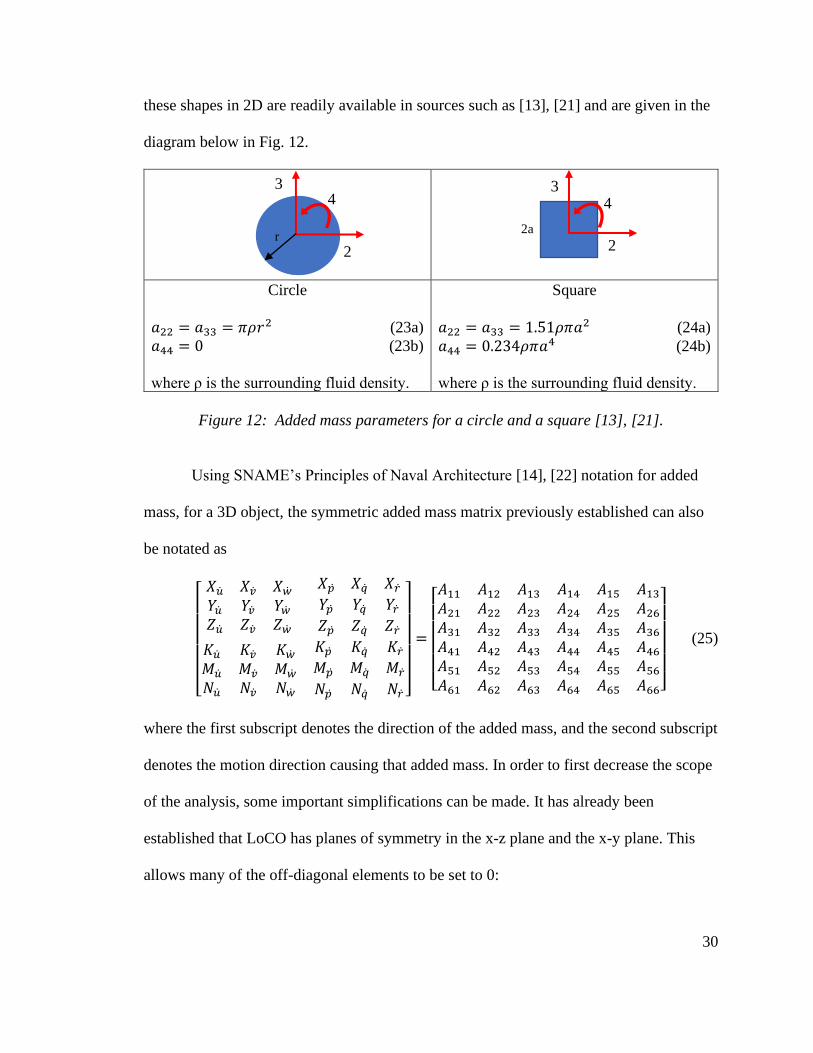
30

these shapes in 2D are readily available in sources such as [13], [21] and are given in the

diagram below in Fig. 12.

Circle

𝑎22 = 𝑎33 = 𝜋𝜌𝑟2 (23a)

𝑎44 = 0 (23b)

where ρ is the surrounding fluid density.

Square

𝑎22 = 𝑎33 = 1.51𝜌𝜋𝑎2 (24a)

𝑎44 = 0.234𝜌𝜋𝑎4 (24b)

where ρ is the surrounding fluid density.

Figure 12: Added mass parameters for a circle and a square [13], [21].

Using SNAME’s Principles of Naval Architecture [14], [22] notation for added

mass, for a 3D object, the symmetric added mass matrix previously established can also

be notated as

[ 𝑋�̇� 𝑋�̇� 𝑋�̇�

𝑌�̇� 𝑌�̇� 𝑌�̇�

𝑍�̇� 𝑍�̇� 𝑍�̇�

𝑋�̇� 𝑋�̇� 𝑋�̇�

𝑌�̇� 𝑌�̇� 𝑌�̇�

𝑍�̇� 𝑍�̇� 𝑍�̇�

𝐾�̇� 𝐾�̇� 𝐾�̇�

𝑀�̇� 𝑀�̇� 𝑀�̇�

𝑁�̇� 𝑁�̇� 𝑁�̇�

𝐾�̇� 𝐾�̇� 𝐾�̇�

𝑀�̇� 𝑀�̇� 𝑀�̇�

𝑁�̇� 𝑁�̇� 𝑁�̇� ]

=

[ 𝐴11 𝐴12 𝐴13

𝐴21 𝐴22 𝐴23

𝐴31 𝐴32 𝐴33

𝐴14 𝐴15 𝐴13

𝐴24 𝐴25 𝐴26

𝐴34 𝐴35 𝐴36

𝐴41 𝐴42 𝐴43

𝐴51 𝐴52 𝐴53

𝐴61 𝐴62 𝐴63

𝐴44 𝐴45 𝐴46

𝐴54 𝐴55 𝐴56

𝐴64 𝐴65 𝐴66]

(25)

where the first subscript denotes the direction of the added mass, and the second subscript

denotes the motion direction causing that added mass. In order to first decrease the scope

of the analysis, some important simplifications can be made. It has already been

established that LoCO has planes of symmetry in the x-z plane and the x-y plane. This

allows many of the off-diagonal elements to be set to 0:

3

2

4 3

2

4

2a r

31

𝑀𝐴 =

[ 𝑋�̇� 0 00 𝑌�̇� 00 0 𝑍�̇�

0 0 00 0 𝑌�̇�

0 𝑍�̇� 0

0 0 00 0 𝑀�̇�

0 𝑁�̇� 0

𝐾�̇� 0 0

0 𝑀�̇� 0

0 0 𝑁�̇�]

(26)

Again from the Principles of Naval Architecture [22], these 3D coefficients can

be obtained from the 2D added mass parameters integrated over the length of the object,

𝐴11 = ∫𝑎11 𝑑𝑥 (27a)

𝐴22 = ∫𝑎22 𝑑𝑥 (27b)

𝐴33 = ∫𝑎33 𝑑𝑥 (27c)

𝐴44 = ∫𝑎44 𝑑𝑥 (27d)

𝐴55 = ∫𝑥2 𝑎33 𝑑𝑥 (27e)

𝐴66 = ∫𝑥2 𝑎22 𝑑𝑥 (27f)

𝐴26 = 𝐴62 = ∫𝑥 𝑎22 𝑑𝑥 (27g)

𝐴35 = 𝐴53 = −∫𝑥 𝑎33 𝑑𝑥 (27h)

Though strip theory makes evaluating added mass parameters in cross flow

possible, axial flow against these cross sections does not have the same sort of available

solutions. One way of estimating this axial added mass due to acceleration along the

same axis is using the approximation for a streamlined body, where such an added mass

is approximately 5 to 10 percent of the mass of the displaced fluid. However, LoCO

cannot necessarily be assumed to be a streamlined body, especially taking the individual

added mass of each thruster into account where those cylinder approximations are more

related to a bluff body.

32

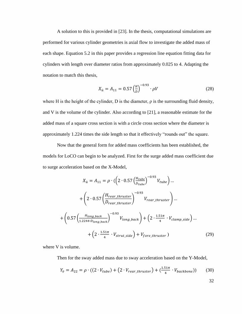
A solution to this is provided in [23]. In the thesis, computational simulations are

performed for various cylinder geometries is axial flow to investigate the added mass of

each shape. Equation 5.2 in this paper provides a regression line equation fitting data for

cylinders with length over diameter ratios from approximately 0.025 to 4. Adapting the

notation to match this thesis,

𝑋�̇� = 𝐴11 = 0.57 (𝐻

𝐷)−0.93

∙ 𝜌𝑉 (28)

where H is the height of the cylinder, D is the diameter, ρ is the surrounding fluid density,

and V is the volume of the cylinder. Also according to [21], a reasonable estimate for the

added mass of a square cross section is with a circle cross section where the diameter is

approximately 1.224 times the side length so that it effectively “rounds out” the square.

Now that the general form for added mass coefficients has been established, the

models for LoCO can begin to be analyzed. First for the surge added mass coefficient due

to surge acceleration based on the X-Model,

𝑋�̇� = 𝐴11 = 𝜌 ∙ ((2 ∙ 0.57 (𝐻𝑡𝑢𝑏𝑒

𝐷𝑡𝑢𝑏𝑒)−0.93

𝑉𝑡𝑢𝑏𝑒)…

+(2 ∙ 0.57 (𝐻𝑟𝑒𝑎𝑟_𝑡ℎ𝑟𝑢𝑠𝑡𝑒𝑟

𝐷𝑟𝑒𝑎𝑟_𝑡ℎ𝑟𝑢𝑠𝑡𝑒𝑟)

−0.93

𝑉𝑟𝑒𝑎𝑟_𝑡ℎ𝑟𝑢𝑠𝑡𝑒𝑟)…

+(0.57 (𝐻𝑙𝑜𝑛𝑔_𝑏𝑎𝑐𝑘

1.2244∙𝐷𝑙𝑜𝑛𝑔_𝑏𝑎𝑐𝑘)−0.93

𝑉𝑙𝑜𝑛𝑔_𝑏𝑎𝑐𝑘) + (2 ∙1.51𝜋

4 ∙ 𝑉𝑐𝑙𝑎𝑚𝑝_𝑠𝑖𝑑𝑒)…

+(2 ∙1.51𝜋

4 ∙ 𝑉𝑠𝑡𝑟𝑢𝑡_𝑠𝑖𝑑𝑒) + 𝑉𝑓𝑜𝑟𝑒_𝑡ℎ𝑟𝑢𝑠𝑡𝑒𝑟 ) (29)

where V is volume.

Then for the sway added mass due to sway acceleration based on the Y-Model,

𝑌�̇� = 𝐴22 = 𝜌 ∙ ((2 ∙ 𝑉𝑡𝑢𝑏𝑒) + (2 ∙ 𝑉𝑟𝑒𝑎𝑟_𝑡ℎ𝑟𝑢𝑠𝑡𝑒𝑟) + (1.51𝜋

4 ∙ 𝑉𝑏𝑎𝑐𝑘𝑏𝑜𝑛𝑒)) (30)

33

and for the heave added mass due to heave acceleration based on the Z-Model,

𝑍�̇� = 𝐴33 = 𝜌 ∙ ((2 ∙ 𝑉𝑡𝑢𝑏𝑒) + (2 ∙ 𝑉𝑟𝑒𝑎𝑟_𝑡ℎ𝑟𝑢𝑠𝑡𝑒𝑟) + (1.51𝜋

4 ∙ 𝑉𝑏𝑎𝑐𝑘𝑏𝑜𝑛𝑒)…

+(1.51𝜋

4 ∙ 𝑉𝑓𝑜𝑟𝑒_𝑐𝑜𝑛𝑛𝑒𝑐𝑡𝑜𝑟) + (

1.51𝜋

4 ∙ 𝑉𝑎𝑓𝑡_𝑐𝑜𝑛𝑛𝑒𝑐𝑡𝑜𝑟)…

+1.51𝜋

4 ∙ 𝑉𝑠𝑡𝑟𝑢𝑡 + (0.57 (

𝐻𝑟𝑒𝑎𝑟_𝑡ℎ𝑟𝑢𝑠𝑡𝑒𝑟

𝐷𝑟𝑒𝑎𝑟_𝑡ℎ𝑟𝑢𝑠𝑡𝑒𝑟)−0.93

𝑉𝑡ℎ𝑟𝑢𝑠𝑡𝑒𝑟) (31)

For the roll added mass coefficient due to roll acceleration, the Z-Model is used

since roll motion offset from the central axis leads to dealing with instantaneous vertical

motion of the individual components. For the backbone, there is already a coefficient a44

that can be applied and integrated over the backbone. For the connectors, strut, and

vertical thruster, roll for the overall underwater vehicle can be expressed equivalent to

pitch about the central axis for each of the components, leading to using equation 27e as

∫ 𝑥2𝑎33𝑑𝑥𝐿𝑒𝑛𝑔𝑡ℎ/2

−𝐿𝑒𝑛𝑔𝑡ℎ/2. The roll added mass for the tubes and rear thrusters can account for

their offset from the roll axis with an appropriate modification of equation 27d, similar to

that of equation 27e,

𝐴44 = ∫𝑟2𝑎33 𝑑𝑥 (32)

where r, in this case, is the perpendicular distance from the central axis to the center of

the cylinders. Using these expressions then,

𝐾�̇� = 𝐴44 = 𝜌 ∙ ((2 ∙ 𝑦𝑐𝑡𝑢𝑏𝑒2 ∙ 𝑉𝑡𝑢𝑏𝑒) + (2 ∙ 𝑦𝑐𝑟𝑒𝑎𝑟_𝑡ℎ𝑟𝑢𝑠𝑡𝑒𝑟

2 ∙ 𝑉𝑟𝑒𝑎𝑟_𝑡ℎ𝑟𝑢𝑠𝑡𝑒𝑟)…

+(𝐻𝑓𝑜𝑟𝑒_𝑡ℎ𝑟𝑢𝑠𝑡𝑒𝑟

2

12∙ 𝑉𝑓𝑜𝑟𝑒_𝑡ℎ𝑟𝑢𝑠𝑡𝑒𝑟) + (

1.51𝜋

4 ∙ 𝑉𝑓𝑜𝑟𝑒_𝑐𝑜𝑛𝑛𝑒𝑐𝑡𝑜𝑟) + (

1.51𝜋


+(1.51𝜋

4 ∙ 𝑉𝑠𝑡𝑟𝑢𝑡 ∙

𝑙𝑒𝑛𝑔𝑡ℎ𝑠𝑡𝑟𝑢𝑡2

12) +

0.234𝜋

4∙ (

𝑤𝑖𝑑𝑡ℎ𝑏𝑎𝑐𝑘𝑏𝑜𝑛𝑒

2)2

∙ 𝑉𝑏𝑎𝑐𝑘𝑏𝑜𝑛𝑒 ) (33)

34

where yc is the geometric center offset in the y direction, length is the length along the

longest axis of the component, and width is the side length of the square cross section.

For the pitch added mass coefficient due to pitch acceleration, the Z-Model is the

most accurate to use again. The added mass coefficients for the tubes, rear thrusters, and

backbone can be determined using the basic formula in equation 27e. For the vertical

thruster, clamp connectors, and rear strut, a modified version of the same equation must

be used considering cross-section propagation is a constant perpendicular distance from

the axis of rotation:

𝐴55 = 𝑟2 ∫𝑎33 𝑑𝑥 (34)

where r in this case is again the perpendicular distance from the axis of rotation to the

corresponding centerline of the rotating component. Overall, then,

𝑀�̇� = 𝐴55 = 𝜌 ∙ ((2 ∙(𝑥2𝑡𝑢𝑏𝑒

3 −𝑥1𝑡𝑢𝑏𝑒3 )

3∙ 𝑆𝑡𝑢𝑏𝑒) …

+(2 ∙(𝑥2𝑟𝑒𝑎𝑟_𝑡ℎ𝑟𝑢𝑠𝑡𝑒𝑟

3 −𝑥1𝑟𝑒𝑎𝑟_𝑡ℎ𝑟𝑢𝑠𝑡𝑒𝑟3 )

3∙ 𝑆𝑟𝑒𝑎𝑟_𝑡ℎ𝑟𝑢𝑠𝑡𝑒𝑟)…

+(0.57 (𝐻𝑡ℎ𝑟𝑢𝑠𝑡𝑒𝑟

𝐷𝑡ℎ𝑟𝑢𝑠𝑡𝑒𝑟)−0.93

∙ 𝑥𝑐𝑓𝑜𝑟𝑒_𝑡ℎ𝑟𝑢𝑠𝑡𝑒𝑟2 ∙ 𝑉𝑓𝑜𝑟𝑒_𝑡ℎ𝑟𝑢𝑠𝑡𝑒𝑟)…

+(1.51𝜋

4 ∙ 𝑥𝑐𝑓𝑜𝑟𝑒_𝑐𝑜𝑛𝑛𝑒𝑐𝑡𝑜𝑟

2 ∙ 𝑉𝑓𝑜𝑟𝑒_𝑐𝑜𝑛𝑛𝑒𝑐𝑡𝑜𝑟)+(1.51𝜋

4 ∙ 𝑥𝑐𝑎𝑓𝑡_𝑐𝑜𝑛𝑛𝑒𝑐𝑡𝑜𝑟


+(1.51𝜋

4 ∙ 𝑥𝑐𝑠𝑡𝑟𝑢𝑡

2 ∙ 𝑉𝑠𝑡𝑟𝑢𝑡) + ((𝑥2𝑏𝑎𝑐𝑘𝑏𝑜𝑛𝑒

3 −𝑥1𝑏𝑎𝑐𝑘𝑏𝑜𝑛𝑒3 )

3∙ 𝑆𝑏𝑎𝑐𝑘𝑏𝑜𝑛𝑒)

where S denotes the cross-sectional reference area, xc is the is the geometric center offset

in the x direction, and x1 and x2 represent the limits of integration performed in the x

direction (from x1 to x2).

For the yaw added mass due to yaw acceleration, the Y-Model is utilized. Though

some components are offset in both the x and y directions, it is assumed that

35

instantaneously, crossflow over the geometry due to yaw is in the y direction since

components are generally more offset from the origin in the x direction than the y

direction. All components for the yaw added mass are computed this way.

𝑁�̇� = 𝐴66 = 𝜌 ∙ ((2 ∙(𝑥2𝑡𝑢𝑏𝑒






+((𝑥2𝑏𝑎𝑐𝑘𝑏𝑜𝑛𝑒


3∙ 𝑆𝑏𝑎𝑐𝑘𝑏𝑜𝑛𝑒) (35)

Now, the off-diagonal elements must be formulated. For the yaw added mass due

to sway acceleration and sway added mass due to yaw acceleration,

𝑌�̇� = 𝑁�̇� = 𝐴26 = 𝜌 ∙ ((2 ∙(𝑥2𝑡𝑢𝑏𝑒






+((𝑥2𝑏𝑎𝑐𝑘𝑏𝑜𝑛𝑒



and with a similar derivation for the heave added mass due to pitch acceleration and pitch

added mass due to heave acceleration,

𝑍�̇� = 𝑀�̇� = 𝐴35 = 𝜌 ∙ ((2 ∙(𝑥2𝑡𝑢𝑏𝑒





2∙ 𝑆𝑡ℎ𝑟𝑢𝑠𝑡𝑒𝑟)…

+(0.57 (𝐻𝑡ℎ𝑟𝑢𝑠𝑡𝑒𝑟

𝐷𝑡ℎ𝑟𝑢𝑠𝑡𝑒𝑟)−0.93

∙ 𝑥𝑐𝑓𝑜𝑟𝑒_𝑡ℎ𝑟𝑢𝑠𝑡𝑒𝑟 ∙ 𝑉𝑟𝑒𝑎𝑟_𝑡ℎ𝑟𝑢𝑠𝑡𝑒𝑟)…

+(1.51𝜋

4 ∙ 𝑥𝑐𝑓𝑜𝑟𝑒_𝑐𝑜𝑛𝑛𝑒𝑐𝑡𝑜𝑟 ∙ 𝑉𝑓𝑜𝑟𝑒_𝑐𝑜𝑛𝑛𝑒𝑐𝑡𝑜𝑟)+(

1.51𝜋

4 ∙ 𝑥𝑐𝑎𝑓𝑡_𝑐𝑜𝑛𝑛𝑒𝑐𝑡𝑜𝑟 ∙ 𝑉𝑎𝑓𝑡_𝑐𝑜𝑛𝑛𝑒𝑐𝑡𝑜𝑟)…

+(1.51𝜋

4 ∙ 𝑥𝑐𝑠𝑡𝑟𝑢𝑡 ∙ 𝑉𝑠𝑡𝑟𝑢𝑡) + (

(𝑥2𝑏𝑎𝑐𝑘𝑏𝑜𝑛𝑒2 −𝑥1𝑏𝑎𝑐𝑘𝑏𝑜𝑛𝑒

2 )


36

Inserting values and solving for each of the parameters gives the following

displayed in Table 4.



Added Mass

𝑋�̇� 2.899 kg

𝑌�̇� 11.855 kg

𝑍�̇� 12.915 kg

𝐾�̇� 0.13557 kg m2

𝑀�̇� 1.4260 kg m2

𝑁�̇� 1.0667 kg m2

𝑍�̇� -3.562 kg m

𝑀�̇� -3.562 kg m

𝑌�̇� 2.818 kg m

𝑁�̇� 2.818 kg m

Table 4: Added mass analysis values.

3.5. Hydrodynamic Damping Coefficients

The first step in determining the hydrodynamic damping parameters on the

underwater vehicle is to determine the relevant coefficients of drag for each geometric

shape involved. Similar to the added mass, in order to analytically approximate the

composite damping coefficients for the vehicle, geometric assumptions must be made.

The X-Model, Y-Model, and Z-Model are used in this analysis as they were with the

added mass.

With a forward top speed of approximately 1.5 meters per second, an overall

length of 0.73 meters, and with the kinematic viscosity of water at 20 degrees Celsius as

1.004*10-6 m2/s [24], the overall Reynolds number of LoCO in forward motion is

𝑅𝑛 =𝑢𝐷

𝜈=

1.5∙0.73

1.004∙10−6 ≈ 106 (38)

37

Intuitively, this value brings the laminar-turbulent flow transition region into question for

evaluating coefficient of drag parameters, since this lies above the typical critical

Reynolds number of ≈ 5 ∙ 105 for a sphere or cylinder in cross flow (See Figs. 11 and 12

in [16]). However, since shorter, individual pieces are being evaluated for drag, and flow

in all directions is not expected to be as high as the very top speed for LoCO, the drag

parameters for the vehicle are assumed to be in the subcritical Reynolds number region.

First, the individual coefficients of drag must be found for each component.

Hoerner [16] is used to provide approximations for all the geometric shapes used, and

figures referenced below are from the same text. As mentioned in the previous section,

the length to diameter ratio for the long tubes is approximately 5, and for the thruster

approximations is about 0.5. Hoerner Figure 3-21 for axial flow across cylindrical bodies

can be used to approximate the total coefficients of drag for these two shapes in axial

flow. This total drag coefficient given includes skin friction effects. This provides an

axial drag coefficient of about 0.8258 for the tubes using the blunt nose line. Though the

thrusters are approximated in shape as blunt cylinders, they do have a short, rounded

portion on either side. In an attempt to account for this, the average of the blunt nose and

streamlined head forms is taken and provides a total axial drag coefficient of

approximately 0.75 for the thrusters. For flow across these same cylinders normal to their

center axis, Hoerner Figure 3-12 for the drag coefficient of a circular cylinder in the same

flow conditions can be used where the 1.2 approximation just before the transition point

is used. Since there is relatively low surface area, skin friction effects are neglected.

The sectional drag coefficient values for the rectangular prisms can be obtained

using Hoerner Figures 3-22 and 3-23. For axial flow with all rectangular prisms, the

38

length to thickness ratio is approximately or above 2.5. So, from Hoerner Figure 3-22, the

total drag coefficient in axial flow is approximately 1 and includes skin friction effects. In

cross flow, the 3D-printed parts have a slight radius on the edges. This ratio of radius to

width of the cross section is about 0.1, so the sectional drag coefficient is approximately

2. Again, as these are bluff bodies in cross flow, the skin friction is considered negligible.

A summary of these drag coefficients are given in Table 5 below.

Component Axial Total CD Cross Flow Total CD

Tube 0.8258 1.2

Thruster 0.75 1.2

Long Backbone 1 Not Needed

Any Square Rectangular Prism (“rect”) Not Needed 2

Table 5: Summary of component coefficients of drag.

Another useful table to express parameters used in determining drag are the

reference areas applicable to the coefficients of drag used in Table 5. Using the

component geometries listed in Table 6,

Component Arefaxial (m2) Cross Flow Arefcross (m2)

Tube 0.010136 0.06109

Thruster 0.007322 0.004291

Long Backbone 0.0017564 Not Needed

Clamp Connectors Not Needed 0.004287

Connector Side Block Not Needed 0.0012655

Strut Side Block Not Needed 0.0016500

Long Backbone Not Needed 0.006094

Rear Strut Not Needed 0.005056

Table 6: Summary of component drag reference areas.

Beginning with the equation for linear drag in the x direction with the X-Model,

39

𝑋𝑢|𝑢| = −1

2 𝜌 (2 ∙ 𝐶𝐷𝑎𝑥𝑖𝑎𝑙𝑡𝑢𝑏𝑒

∙ 𝐴𝑟𝑒𝑓𝑎𝑥𝑖𝑎𝑙𝑡𝑢𝑏𝑒+ 2 ∙ 𝐶𝐷_𝑎𝑥𝑖𝑎𝑙𝑡ℎ𝑟𝑢𝑠𝑡𝑒𝑟

∙ 𝐴𝑟𝑒𝑓𝑎𝑥𝑖𝑎𝑙𝑡ℎ𝑟𝑢𝑠𝑡𝑒𝑟…

+𝐶𝐷𝑐𝑟𝑜𝑠𝑠𝑡ℎ𝑟𝑢𝑠𝑡𝑒𝑟∙ 𝐴𝑟𝑒𝑓𝑐𝑟𝑜𝑠𝑠𝑡ℎ𝑟𝑢𝑠𝑡𝑒𝑟

+𝐶𝐷𝑎𝑥𝑖𝑎𝑙𝑙𝑜𝑛𝑔_𝑏𝑎𝑐𝑘∙ 𝐴𝑟𝑒𝑓𝑎𝑥𝑖𝑎𝑙𝑙𝑜𝑛𝑔_𝑏𝑎𝑐𝑘

…

+2 ∙ 𝐶𝐷𝑐𝑟𝑜𝑠𝑠𝑟𝑒𝑐𝑡∙ 𝐴𝑟𝑒𝑓𝑐𝑟𝑜𝑠𝑠𝑐𝑜𝑛𝑛𝑒𝑐𝑡𝑜𝑟_𝑠𝑖𝑑𝑒

…

+2 ∙ 𝐶𝐷𝑐𝑟𝑜𝑠𝑠𝑟𝑒𝑐𝑡∙ 𝐴𝑟𝑒𝑓𝑐𝑟𝑜𝑠𝑠𝑠𝑡𝑟𝑢𝑡_𝑠𝑖𝑑𝑒

) (39)

Due to symmetry, drag caused by motion in the x direction does not also cause a

net yaw moment on the model. Then for the lateral direction with the Y-Model,

𝑌𝑣|𝑣| = −1

2 𝜌 (2 ∙ 𝐶𝐷𝑐𝑟𝑜𝑠𝑠𝑡𝑢𝑏𝑒

∙ 𝐴𝑟𝑒𝑓𝑐𝑟𝑜𝑠𝑠𝑡𝑢𝑏𝑒+ 2 ∙ 𝐶𝐷_𝑐𝑟𝑜𝑠𝑠𝑡ℎ𝑟𝑢𝑠𝑡𝑒𝑟

∙ 𝐴𝑟𝑒𝑓𝑐𝑟𝑜𝑠𝑠𝑡ℎ𝑟𝑢𝑠𝑡𝑒𝑟…

+𝐶𝐷𝑐𝑟𝑜𝑠𝑠𝑏𝑎𝑐𝑘𝑏𝑜𝑛𝑒∙ 𝐴𝑟𝑒𝑓𝑐𝑟𝑜𝑠𝑠𝑏𝑎𝑐𝑘𝑏𝑜𝑛𝑒

) (40)

With this, there is also a net yaw drag moment caused by linear motion in the y

direction. With each coefficient tied to a force in the y direction, the coefficient for each

component can be multiplied by its center offset in the x direction causing rotation about

the yaw axis,

𝑁𝑣|𝑣| =1

2 𝜌 (−2 ∙ 𝐶𝐷𝑐𝑟𝑜𝑠𝑠𝑡𝑢𝑏𝑒

∙ 𝐴𝑟𝑒𝑓𝑐𝑟𝑜𝑠𝑠𝑡𝑢𝑏𝑒∙ 𝑥𝑐𝑡𝑢𝑏𝑒 …

+2 ∙ 𝐶𝐷_𝑐𝑟𝑜𝑠𝑠𝑡ℎ𝑟𝑢𝑠𝑡𝑒𝑟∙ 𝐴𝑟𝑒𝑓𝑐𝑟𝑜𝑠𝑠𝑡ℎ𝑟𝑢𝑠𝑡𝑒𝑟

∙ 𝑥𝑐𝑟𝑒𝑎𝑟_𝑡ℎ𝑟𝑢𝑠𝑡𝑒𝑟 …


∙ 𝑥𝑐𝑏𝑎𝑐𝑘𝑏𝑜𝑛𝑒) (41)

And finally in the vertical direction using the Z-Model,

𝑍𝑤|𝑤| = −1


∙ 𝐴𝑟𝑒𝑓𝑐𝑟𝑜𝑠𝑠𝑡𝑢𝑏𝑒+ 𝐶𝐷𝑎𝑥𝑖𝑎𝑙𝑡ℎ𝑟𝑢𝑠𝑡𝑒𝑟

∙ 𝐴𝑟𝑒𝑓𝑎𝑥𝑖𝑎𝑙𝑡ℎ𝑟𝑢𝑠𝑡𝑒𝑟…

+2 ∙ 𝐶𝐷𝑐𝑟𝑜𝑠𝑠𝑡ℎ𝑟𝑢𝑠𝑡𝑒𝑟∙ 𝐴𝑟𝑒𝑓𝑐𝑟𝑜𝑠𝑠𝑡ℎ𝑟𝑢𝑠𝑡𝑒𝑟


…

+2 ∙ 𝐶𝐷𝑐𝑟𝑜𝑠𝑠𝑐𝑜𝑛𝑛𝑒𝑐𝑡𝑜𝑟∙ 𝐴𝑟𝑒𝑓𝑐𝑟𝑜𝑠𝑠𝑐𝑜𝑛𝑛𝑒𝑐𝑡𝑜𝑟

…

+𝐶𝐷𝑐𝑟𝑜𝑠𝑠𝑠𝑡𝑟𝑢𝑡∙ 𝐴𝑟𝑒𝑓𝑐𝑟𝑜𝑠𝑠𝑠𝑡𝑟𝑢𝑡

) (42)

40

There is also a net pitch drag moment caused by linear motion in the z direction.

With each coefficient tied to a force in the z direction, the coefficient for each component

can be multiplied by its center offset in the x direction causing rotation about the pitch

axis,

𝑀𝑤|𝑤| =1


∙ 𝐴𝑟𝑒𝑓𝑐𝑟𝑜𝑠𝑠𝑡𝑢𝑏𝑒∙ 𝑥𝑐𝑡𝑢𝑏𝑒 …

+𝐶𝐷𝑎𝑥𝑖𝑎𝑙𝑡ℎ𝑟𝑢𝑠𝑡𝑒𝑟∙ 𝐴𝑟𝑒𝑓𝑎𝑥𝑖𝑎𝑙𝑡ℎ𝑟𝑢𝑠𝑡𝑒𝑟

∙ 𝑥𝑐𝑓𝑜𝑟𝑒_𝑡ℎ𝑟𝑢𝑠𝑡𝑒𝑟 …


∙ 𝑥𝑐𝑟𝑒𝑎𝑟_𝑡ℎ𝑟𝑢𝑠𝑡𝑒𝑟 …


∙ 𝑥𝑐𝑏𝑎𝑐𝑘𝑏𝑜𝑛𝑒 …

+2 ∙ 𝐶𝐷𝑐𝑟𝑜𝑠𝑠𝑐𝑜𝑛𝑛𝑒𝑐𝑡𝑜𝑟∙ 𝐴𝑟𝑒𝑓𝑐𝑟𝑜𝑠𝑠𝑐𝑜𝑛𝑛𝑒𝑐𝑡𝑜𝑟

∙ 𝑥𝑐𝑐𝑜𝑛𝑛𝑒𝑐𝑡𝑜𝑟 …

+𝐶𝐷𝑐𝑟𝑜𝑠𝑠𝑠𝑡𝑟𝑢𝑡∙ 𝐴𝑟𝑒𝑓𝑐𝑟𝑜𝑠𝑠𝑠𝑡𝑟𝑢𝑡

∙ 𝑥𝑐𝑠𝑡𝑟𝑢𝑡) (43)

Now the moment damping coefficients must be determined. For roll damping, the

Z-Model can be used. The damping with the rotation of the backbone and vertical

thruster through their center axes may be neglected. For the tubes and rear thrusters, a roll

motion can be approximated as instantaneously vertical motion at a distance away from

the roll axis. Rather than the typical integral expression in equation 16 that will be used

for the clamp connectors and the rear strut, this moment damping can be expressed as

𝑀𝐷 = 𝐹𝐷 ⊥ 𝑟 = −1

2𝜌𝐶𝐷(𝑅𝑛)𝐴𝑟𝑒𝑓|𝜔|𝜔 ∙ 𝑟2|𝑟| (44)

where r is the perpendicular distance from the axis of rotation. Expressing the roll

damping coefficient,

𝐾𝑝|𝑝| = −1


∙ 𝐴𝑟𝑒𝑓𝑐𝑟𝑜𝑠𝑠𝑡𝑢𝑏𝑒∙ 𝑦𝑐𝑡𝑢𝑏𝑒

3 …


∙ 𝑦𝑐𝑟𝑒𝑎𝑟_𝑡ℎ𝑟𝑢𝑠𝑡𝑒𝑟3 …

41

+𝐶𝐷𝑐𝑟𝑜𝑠𝑠𝑐𝑜𝑛𝑛𝑒𝑐𝑡𝑜𝑟∙ 𝑤𝑖𝑑𝑡ℎ𝑐𝑜𝑛𝑛𝑒𝑐𝑡𝑜𝑟 ∙

(𝑙𝑒𝑛𝑔𝑡ℎ𝑐𝑜𝑛𝑛𝑒𝑐𝑡𝑜𝑟/2)4

4…

+𝐶𝐷𝑐𝑟𝑜𝑠𝑠𝑠𝑡𝑟𝑢𝑡∙ 𝑤𝑖𝑑𝑡ℎ𝑠𝑡𝑟𝑢𝑡 ∙

(𝑙𝑒𝑛𝑔𝑡ℎ𝑠𝑡𝑟𝑢𝑡/2)4

4 ) (45)

Next is the pitch damping coefficient for the underwater vehicle using the Z-

Model. In this motion, the moments for the tubes, rear thrusters, and backbone must be

integrated as in equation 16, but the remaining components utilize the modified equation

44.

𝑀𝑞|𝑞| = −1

2 𝜌 ∙ ((2 ∙ 𝐶𝐷𝑐𝑟𝑜𝑠𝑠𝑡𝑢𝑏𝑒

∙ 𝑤𝑖𝑑𝑡ℎ𝑡𝑢𝑏𝑒 ∙(𝑥2𝑡𝑢𝑏𝑒

3 |𝑥2𝑡𝑢𝑏𝑒|−𝑥1𝑡𝑢𝑏𝑒3 |𝑥1𝑡𝑢𝑏𝑒|)

4) …

+(2 ∙ 𝐶𝐷𝑐𝑟𝑜𝑠𝑠𝑡ℎ𝑟𝑢𝑠𝑡𝑒𝑟∙ 𝐻𝑡ℎ𝑟𝑢𝑠𝑡𝑒𝑟 ∙

(𝑥2𝑟𝑒𝑎𝑟_𝑡ℎ𝑟𝑢𝑠𝑡𝑒𝑟3 |𝑥2𝑟𝑒𝑎𝑟_𝑡ℎ𝑟𝑢𝑠𝑡𝑒𝑟|−𝑥1𝑟𝑒𝑎𝑟_𝑡ℎ𝑟𝑢𝑠𝑡𝑒𝑟

3 |𝑥1𝑟𝑒𝑎𝑟_𝑡ℎ𝑟𝑢𝑠𝑡𝑒𝑟|)

4)…

+(𝐶𝐷𝑐𝑟𝑜𝑠𝑠𝑏𝑎𝑐𝑘𝑏𝑜𝑛𝑒∙ 𝑙𝑒𝑛𝑔𝑡ℎ𝑏𝑎𝑐𝑘𝑏𝑜𝑛𝑒 ∙

(𝑥2𝑏𝑎𝑐𝑘𝑏𝑜𝑛𝑒3 |𝑥2𝑏𝑎𝑐𝑘𝑏𝑜𝑛𝑒|−𝑥1𝑏𝑎𝑐𝑘𝑏𝑜𝑛𝑒

3 |𝑥1𝑏𝑎𝑐𝑘𝑏𝑜𝑛𝑒|)

4)…

+(𝐶𝐷𝑎𝑥𝑖𝑎𝑙𝑡ℎ𝑟𝑢𝑠𝑡𝑒𝑟∙ 𝐴𝑟𝑒𝑓𝑎𝑥𝑖𝑎𝑙𝑡ℎ𝑟𝑢𝑠𝑡𝑒𝑟

∙ 𝑥𝑐𝑓𝑜𝑟𝑒_𝑡ℎ𝑟𝑢𝑠𝑡𝑒𝑟3 )…

+(𝐶𝐷𝑐𝑟𝑜𝑠𝑠𝑐𝑜𝑛𝑛𝑒𝑐𝑡𝑜𝑟∙ 𝐴𝑟𝑒𝑓𝑐𝑟𝑜𝑠𝑠𝑐𝑜𝑛𝑛𝑒𝑐𝑡𝑜𝑟

∙ 𝑥𝑐𝑓𝑜𝑟𝑒_𝑐𝑜𝑛𝑛𝑒𝑐𝑡𝑜𝑟3 )…

+(𝐶𝐷𝑐𝑟𝑜𝑠𝑠𝑐𝑜𝑛𝑛𝑒𝑐𝑡𝑜𝑟∙ 𝐴𝑟𝑒𝑓𝑐𝑟𝑜𝑠𝑠𝑐𝑜𝑛𝑛𝑒𝑐𝑡𝑜𝑟

∙ 𝑥𝑐𝑎𝑓𝑡_𝑐𝑜𝑛𝑛𝑒𝑐𝑡𝑜𝑟3 )…

+(𝐶𝐷𝑐𝑟𝑜𝑠𝑠𝑠𝑡𝑟𝑢𝑡∙ 𝐴𝑟𝑒𝑓𝑐𝑟𝑜𝑠𝑠𝑠𝑡𝑟𝑢𝑡

∙ |𝑥𝑐𝑠𝑡𝑟𝑢𝑡3 |) (46)

Finally for the yaw damping coefficient using the Y-Model, all components must

be integrated using equation 16. As explained with the yaw added mass, it is assumed

that yaw motion produces an instantaneous velocity in the y direction, so component

offsets in the x direction cancel and are not considered.

43

Mass m 12.545 kg

Weight W 123.02 N

Center of Gravity

CGx 0.2417 m

CGy 0 m

CGz 0 m

Moments of Inertia

Ix 0.19094 kg m2

Iy 1.2050 kg m2

Iz 1.3465 kg m2

Ixy 0 kg m2

Iyz 0 kg m2

Ixz 0 kg m2

Added Mass

𝑋�̇� 2.899 kg

𝑌�̇� 11.855 kg

𝑍�̇� 12.915 kg

𝐾�̇� 0.13557 kg m2

𝑀�̇� 1.4260 kg m2

𝑁�̇� 1.0667 kg m2

𝑍�̇� -3.562 kg m

𝑀�̇� -3.562 kg m

𝑌�̇� 2.818 kg m

𝑁�̇� 2.818 kg m

Hydrodynamic Damping

Coefficients

𝑋𝑢|𝑢| -23.14 kg/m

𝑌𝑣|𝑣| -84.56 kg/m

𝑍𝑤|𝑤| -100.93 kg/m

𝐾𝑝|𝑝| -0.09952 kg m2

𝑀𝑞|𝑞| -3.237 kg m2

𝑁𝑟|𝑟| -2.831 kg m2

𝑀𝑤|𝑤| 20.55 kg

𝑁𝑣|𝑣| -18.60 kg

Relevant Thruster Offsets

xcfore 0.4156 m

ycport -0.10932 m

ycstarboard 0.10932 m

Table 8: Relevant dynamic model parameters from analysis and estimation.

Expressing the final dynamic equations for LoCO,

Surge

𝑚(�̇� − 𝑣𝑟 + 𝑤𝑞 − 𝑥𝐺(𝑞2 + 𝑟2)) = 𝑇𝑝𝑜𝑟𝑡 + 𝑇𝑠𝑡𝑏𝑑 + 𝑋𝑢|𝑢|𝑢|𝑢|…

−(𝑋�̇��̇� + 𝑍�̇�𝑤𝑞 + 𝑍�̇�𝑞2 − 𝑌�̇�𝑣𝑟 − 𝑌�̇�𝑟

2) (48a)

44

Sway

𝑚(�̇� − 𝑤𝑝 + 𝑢𝑟 + 𝑥𝐺(𝑞𝑝 + �̇�)) = 𝑌𝑣|𝑣|𝑣|𝑣|…

−(𝑌�̇��̇� + 𝑌�̇��̇� + 𝑋�̇�𝑢𝑟 − 𝑍�̇�𝑤𝑝−𝑍�̇�𝑝𝑞) (48b)

Heave

𝑚(�̇� − 𝑢𝑞 + 𝑣𝑝 + 𝑥𝐺(𝑟𝑝 − �̇�)) = 𝑇𝑓𝑜𝑟𝑒 + 𝑍𝑤|𝑤|𝑤|𝑤|…

−(𝑍�̇��̇� + 𝑍�̇��̇� − 𝑋�̇�𝑢𝑞 + 𝑌�̇�𝑣𝑝 + 𝑌�̇�𝑟𝑝) (48c)

Roll

𝐼𝑥�̇� + (𝐼𝑧 − 𝐼𝑦)𝑞𝑟 = 𝐾𝑝|𝑝|𝑝|𝑝|…

−(𝐾�̇��̇� − (𝑌�̇� − 𝑍�̇�)𝑣𝑤 − (𝑌�̇� + 𝑍�̇�)𝑤𝑟 + (𝑌�̇� + 𝑍�̇�)𝑣𝑞 − (𝑀�̇� − 𝑁�̇�)𝑞𝑟) (48d)

Pitch

𝐼𝑦�̇� + (𝐼𝑥 − 𝐼𝑧)𝑟𝑝 + 𝑚(−𝑥𝐺(�̇� − 𝑢𝑞 + 𝑣𝑝)) = −𝑇𝑓𝑜𝑟𝑒 𝑥𝑐𝑓𝑜𝑟𝑒 …

+𝑀𝑞|𝑞|𝑞|𝑞|+𝑀𝑤|𝑤|𝑤|𝑤| − (𝑍�̇�(�̇� − 𝑢𝑞) + 𝑀�̇��̇� − (𝑍�̇� − 𝑋�̇�)𝑤𝑢 …

−𝑌�̇�𝑣𝑝 + (𝐾�̇� − 𝑁�̇�)𝑟𝑝) (48e)

Yaw

𝐼𝑧�̇� + (𝐼𝑦 − 𝐼𝑥)𝑝𝑞 + 𝑚(𝑥𝐺(�̇� − 𝑤𝑝 + 𝑢𝑟)) = −𝑇𝑝𝑜𝑟𝑡 𝑦𝑐𝑝𝑜𝑟𝑡 − 𝑇𝑠𝑡𝑏𝑑 𝑦𝑐𝑠𝑡𝑏𝑑 …

+𝑁𝑟|𝑟|𝑟|𝑟|+𝑁𝑣|𝑣|𝑣|𝑣| − (𝑌�̇��̇� + 𝑁�̇��̇� − (𝑋�̇� − 𝑌�̇�)𝑢𝑣 + 𝑌�̇�𝑢𝑟 + 𝑍�̇�𝑤𝑝…

−(𝐾�̇� − 𝑀�̇�)𝑝𝑞) (48f)

3.7. Conclusion

In this chapter, the various physical and hydrodynamic values for LoCO have

been determined. Parameters relating to buoyancy were determined using analytical

methods and the CAD model of LoCO. Mass and moment of inertia values were also

45

obtained using the CAD model of LoCO along with computational estimation, analytical

methods, and physical measurements. General assumptions have been made for each of

these cases in order to simplify the governing dynamic models of the underwater vehicle.

The more complex geometry of LoCO was simplified into three different geometric

models that attempt to approximate added mass and hydrodynamic damping measures

based on a composite makeup of simpler shapes. Final parametrized dynamic equations

for LoCO are presented that allow the next step in simulating the AUV.

46

Chapter 4

Simulation

4.1. Introduction

There are a number of different simulation software programs that can be used in

a dynamic simulation of a rigid body, such as Matlab or Unreal Engine. However, a

simulation program that is able to directly interface with LoCO’s software and Robot

Operating System (ROS) framework is Gazebo [25]. Like ROS, Gazebo is an open-

source platform for robotics and other software development that enables the

visualization and physics simulation of robots without requiring real-world testing. This

is especially valuable in the field of underwater robotics with a relatively unforgiving

environment in the case of equipment failures.

4.2. Modeling and Visualization

The modeling and visualization of LoCO in the simulation software is based on

the SolidWorks CAD design model as seen earlier in the thesis. It is used as the template

for creating the Universal Robotic Description Format (URDF) file for the robot, which is

an XML-based file format for representing the model of a robot. Components of the robot

are connected to the main robot frame or other components through “links”, like the

linkages of a robot arm. The inertial matrix for LoCO is based on the estimates made in

Chapter 3, along with its mass. In order to improve the efficiency of the simulation

without affecting the physics engine, the mesh file generated by SolidWorks to provide

the visual representation of LoCO does not include internal components. This physical

47

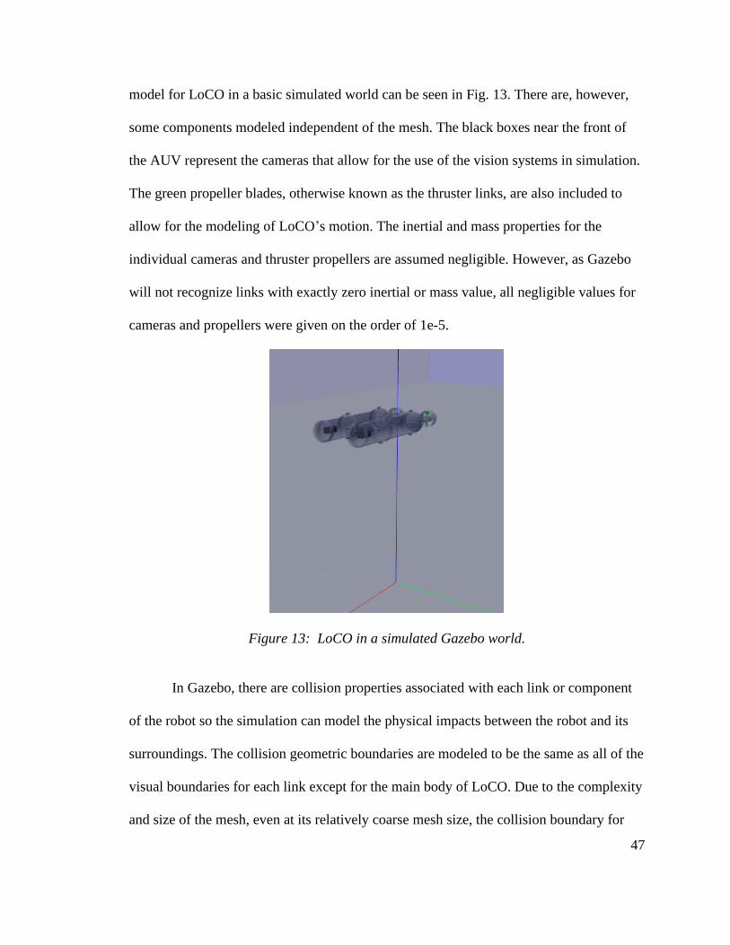
model for LoCO in a basic simulated world can be seen in Fig. 13. There are, however,

some components modeled independent of the mesh. The black boxes near the front of

the AUV represent the cameras that allow for the use of the vision systems in simulation.

The green propeller blades, otherwise known as the thruster links, are also included to

allow for the modeling of LoCO’s motion. The inertial and mass properties for the

individual cameras and thruster propellers are assumed negligible. However, as Gazebo

will not recognize links with exactly zero inertial or mass value, all negligible values for

cameras and propellers were given on the order of 1e-5.

Figure 13: LoCO in a simulated Gazebo world.

In Gazebo, there are collision properties associated with each link or component

of the robot so the simulation can model the physical impacts between the robot and its

surroundings. The collision geometric boundaries are modeled to be the same as all of the

visual boundaries for each link except for the main body of LoCO. Due to the complexity

and size of the mesh, even at its relatively coarse mesh size, the collision boundary for

48

the main body is modeled as a box so as to lower the computational requirements of the

simulation. The GazeboRosControl plugin is also incorporated in the URDF file to load

appropriate hardware interfaces, control managers, and transmission tags into Gazebo for

simulation.

4.3. Physics

The physics engine implemented in Gazebo is the Open Dynamics Engine (ODE)

[26]. Fluid mechanics and other real-world forces are not directly simulated in Gazebo.

Instead, the hydrodynamic forces must be calculated within a ROS node then applied to

the underwater vehicle model. First, in general, the ODE physics engine automatically

applies a standard gravitational force to the model. With LoCO neutrally buoyant, a

Gazebo plugin called “BuoyancyPlugin” applies the appropriate buoyancy force based on

the specified water density and volume of the model. Although the displacement volume

of LoCO has already been estimated, a volume made to match the collision bounding box

is set in the model to achieve neutral buoyancy.

There are a number of ways to simulate LoCO’s propeller propulsion. For

example, there is the Gazebo LiftDragPlugin that computes the thrust generated by

spinning airfoils of given properties, or there are direct ROS Twist messages that can be

sent to the simulation that directly control the velocity of the thrusters. However, with the

established assumption that the thrusters provide point forces, the GazeboRosForce

plugin was implemented to directly apply thruster forces to each of the thrusters. The

simple physical models for the propellers have been left in the simulation in the case of

future propeller dynamics integration. The underwater thrust force data for the T100

49

thruster from Blue Robotics is readily available on their website and discussed further in

Chapter 5.

However, issues with ROS communication arose with this approach. Messages

sent to the simulation to apply forces to the thrusters are only sent one at a time.

Theoretically, the messages are all sent simultaneously, but even with only slight

computation delay, certain LoCO motions cause a buildup in robot movement error. So, it

was determined that all forces and moments on the robot would be summed and applied

to vehicle frame origin through the same GazeboRosForce plugin as described in Chapter

3.

4.4. Simulation Architecture and Control

This ROS node graph in Fig. 14 shows the main working parts of the simulation,

but the three critical aspects are the teleop keyboard program on the left, the sim control

node program in the middle, and the Gazebo simulation on the right. The teleop keyboard

is a program that sends the simulated robot thruster commands based on keyboard input.

The Gazebo component on the far right is the actual simulation, where force commands

and physics are applied to the robot. The sim control node highlighted in red is what

bridges existing LoCO software with the simulation. It reads in the commands from the

teleop node, reads in the state of the robot from Gazebo, then performs the necessary

rotations to the force vectors and applies these to the simulation model.

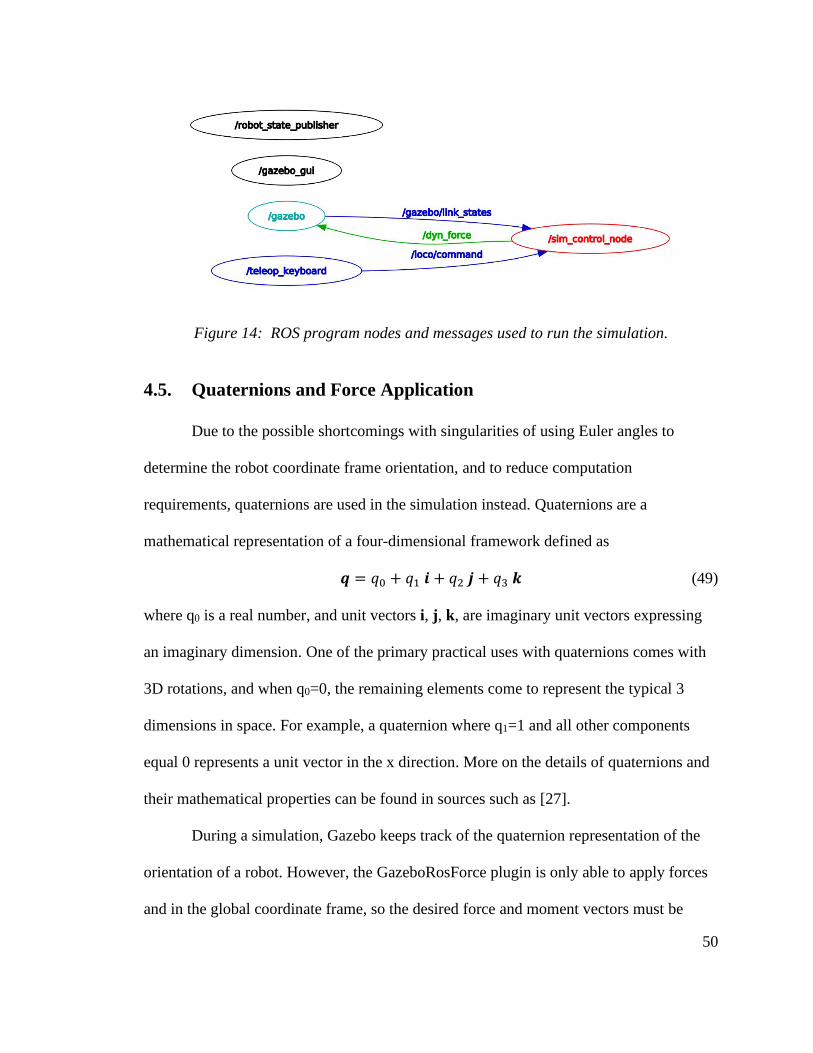
50

Figure 14: ROS program nodes and messages used to run the simulation.

4.5. Quaternions and Force Application

Due to the possible shortcomings with singularities of using Euler angles to

determine the robot coordinate frame orientation, and to reduce computation

requirements, quaternions are used in the simulation instead. Quaternions are a

mathematical representation of a four-dimensional framework defined as

𝒒 = 𝑞0 + 𝑞1 𝒊 + 𝑞2 𝒋 + 𝑞3 𝒌 (49)

where q0 is a real number, and unit vectors i, j, k, are imaginary unit vectors expressing

an imaginary dimension. One of the primary practical uses with quaternions comes with

3D rotations, and when q0=0, the remaining elements come to represent the typical 3

dimensions in space. For example, a quaternion where q1=1 and all other components

equal 0 represents a unit vector in the x direction. More on the details of quaternions and

their mathematical properties can be found in sources such as [27].

During a simulation, Gazebo keeps track of the quaternion representation of the

orientation of a robot. However, the GazeboRosForce plugin is only able to apply forces

and in the global coordinate frame, so the desired force and moment vectors must be

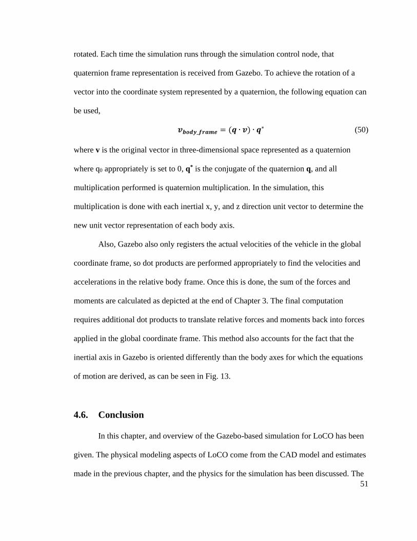
51

rotated. Each time the simulation runs through the simulation control node, that

quaternion frame representation is received from Gazebo. To achieve the rotation of a

vector into the coordinate system represented by a quaternion, the following equation can

be used,

𝒗𝒃𝒐𝒅𝒚_𝒇𝒓𝒂𝒎𝒆 = (𝒒 ∙ 𝒗) ∙ 𝒒∗ (50)

where v is the original vector in three-dimensional space represented as a quaternion

where q0 appropriately is set to 0, q* is the conjugate of the quaternion q, and all

multiplication performed is quaternion multiplication. In the simulation, this

multiplication is done with each inertial x, y, and z direction unit vector to determine the

new unit vector representation of each body axis.

Also, Gazebo also only registers the actual velocities of the vehicle in the global

coordinate frame, so dot products are performed appropriately to find the velocities and

accelerations in the relative body frame. Once this is done, the sum of the forces and

moments are calculated as depicted at the end of Chapter 3. The final computation

requires additional dot products to translate relative forces and moments back into forces

applied in the global coordinate frame. This method also accounts for the fact that the

inertial axis in Gazebo is oriented differently than the body axes for which the equations

of motion are derived, as can be seen in Fig. 13.

4.6. Conclusion

In this chapter, and overview of the Gazebo-based simulation for LoCO has been

given. The physical modeling aspects of LoCO come from the CAD model and estimates

made in the previous chapter, and the physics for the simulation has been discussed. The

52

basic control framework for the simulation is based on ROS nodes and is made to allow

an interface between existing LoCO software and the simulation world. Finally,

quaternion rotations are used to correctly apply forces to the robot model for

computational efficiency and regardless of the model state.

53

Chapter 5

Experimental Data and Comparison with Simulation

5.1. Introduction

Though analytical modeling and simulations can be performed to approximate the

dynamic properties of a vehicle, real world testing is still critical. For full scale ships,

dynamic characterization is often performed on a scale model in a tow tank that can

maintain a given set of motions. The experimental testing with LoCO, however, occurred

within a pool setting during a regular trial period. The currently available motion set of

data is for straight line, horizontal motion at various thruster throttle commands.

5.2. Experiment and Data Analysis

Since the forward motion of an underwater vehicle is arguably the most critical

and simplest motion to test, this serves as the starting point for experimental data. Inertial

measurement unit (IMU) data was collected at various equal rear thruster forces to

provide a range of steady state velocities for LoCO. Each test case was repeated and

averaged in order to confirm results.

The test cases for the experiment were based on throttle command, or a proportion

of the maximum pulse width modulator (PWM) input to the electronic speed controller.

The published thrust data for the T100 Blue Robotics thrusters can be seen below in Fig.

15 [28]. Throttle commands range from -1 to 1, with a command of 0 centered at an input

of 1500 μs. For example, a throttle command of 0.5 translates to 1700 μs. This

54

relationship was used to translate throttle command data into an axial force exerted by the

thrusters on the robot.

Figure 15: Thruster force versus PWM input [28].

IMU data was logged with the Pixhawk through the Mavros ROS package.

Though tests were designed to be straight and horizontal, there was inevitably some

variability in the robot motion, primarily a slight net pitching moment due to water

seeping into some of the rear 3D printed components at the time. Conveniently, the

Mavros package also provides the quaternion coordinate frame state of the robot on top

of the acceleration data. So, like the frame rotations described in Section 4.5, any effect

of the acceleration due to gravity on acceleration in the relative forward direction of the

robot is filtered out. Maximum forward velocity for each throttle case was determined

through trapezoidal integration of IMU acceleration data from the test start through the

55

point where steady state was reached. The results of this data analysis are shown in the

following section.

5.3. Simulation Data Comparison

With experimental data gathered for the forward motion case, the simulation can

be compared to real data. Tests equivalent to the ones performed in the pool were

performed in simulation for horizontal, straight line LoCO motion.

Figure 16: Velocity versus forward thrust applied for a straight line, horizontal path in a

pool.

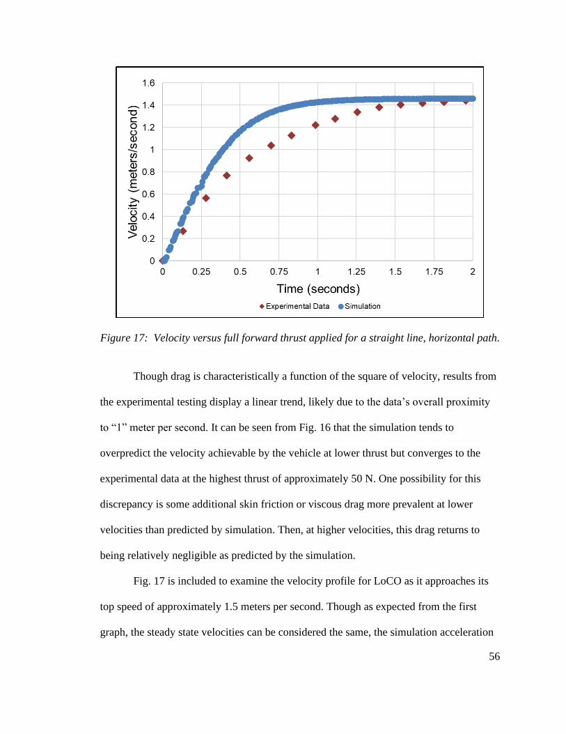
56

Figure 17: Velocity versus full forward thrust applied for a straight line, horizontal path.

Though drag is characteristically a function of the square of velocity, results from

the experimental testing display a linear trend, likely due to the data’s overall proximity

to “1” meter per second. It can be seen from Fig. 16 that the simulation tends to

overpredict the velocity achievable by the vehicle at lower thrust but converges to the

experimental data at the highest thrust of approximately 50 N. One possibility for this

discrepancy is some additional skin friction or viscous drag more prevalent at lower

velocities than predicted by simulation. Then, at higher velocities, this drag returns to

being relatively negligible as predicted by the simulation.

Fig. 17 is included to examine the velocity profile for LoCO as it approaches its

top speed of approximately 1.5 meters per second. Though as expected from the first

graph, the steady state velocities can be considered the same, the simulation acceleration

57

is higher than the experimental data. Part of this may be due to the higher drag than

expected at lower velocities as seen in the Fig. 15. Another possibility is that the added

mass estimates made from Equation 28 resulting from computational fluid dynamics

simulations in [23] could tend to be lower than actual results. A higher added mass would

also effectively decrease the acceleration of the vehicle and bring the simulation curve

down to the experimental data.

Since experimental data was only gathered for surge motion, comparisons are not

able to be made between the dynamic model and real-word data for other motions, such

as yaw or pitching in the vertical plane. Further analysis and testing are required to verify

the presented dynamic modeling for LoCO.

5.4. Conclusion

Experimental trials have been run for LoCO’s motion in horizontal, straight paths.

Forward acceleration relative to the vehicle was isolated during analysis by filtering data

with quaternion rotation. This testing has established a maximum speed of approximately

1.5 meters per second and provided overall estimates on forward velocity profiles.

Simulation data for the same type of motion has been gathered and compared to the

experimental results. Though the maximum velocity for LoCO in simulation correlates

well to real data, the simulation typically leads to higher predicted velocities at lower

thrusts than seen in experiments. This leads to suspected drag forces at lower velocities

not currently accounted for tin the simulation. Further testing is required in order to

validate the dynamic modeling for other LoCO motions, such as pitch and yaw.

58

Chapter 6

Conclusion

6.1. Review

In this thesis, the dynamic modeling and simulation of the LoCO AUV has been

presented. An introduction to LoCO is given, following by the establishment of a

foundation for dynamic derivations. The equations of motion for LoCO in 6 DOF are

derived, and the corresponding forces are brought to attention in Chapter 2. The

following chapter goes on to evaluate the presented coefficients and constants associated

with the geometry of LoCO. The resulting finalized dynamic equations are implemented

in a Gazebo-based simulator that is able to interface with onboard robot software.

Chapter 5 presents the testing performed to obtain experimental surge data for LoCO’s

motion. An overview of the data analysis is given and compared to equivalent simulation

experiment data.

6.2. Conclusions

Overall, this thesis sought to derive the dynamic equations for an underwater

vehicle such as LoCO and evaluate the geometric-dependent parameters using established

assumptions. Further, the model was to be implemented in a simulation and compared

with experimental data obtained in a pool trial. The thesis has been primarily successful

in all these points, but more analysis and real-world testing is required to firmly validate

the full dynamic model for the vehicle.

59

6.3. Future Work

From this work, the foundation for dynamic characterization of the vehicle is

established. Autonomous behavior and control system development can use the

developed models to improve LoCO’s ability to perform underwater operations and assist

personnel. Also, the dynamic models have been derived with respect to the rear of the

tubes on the robot, rather than the center of gravity, which can certainly change as the

robot development is continued. This allows for the easiest possible future modification

of the dynamic models presented herein as the robot changes and additional equipment or

sensors are implemented.

60

References

[1] A. B. Rechnitzer and J. D. Baker, “Undersea exploration,” Encyclopedia

Britannica. 2017.

[2] M. Sahi, “Challenges for Underwater Robotics,” 2015. [Online]. Available:

https://www.tractica.com/automation-robotics/challenges-for-underwater-robots/.

[Accessed: 12-Oct-2019].

[3] C. C. Eriksen et al., “Seaglider : A Long-Range Autonomous Underwater Vehicle

for Oceanographic Research,” IEEE J. Ocean. Eng., vol. 26, no. 4, pp. 424–436,

2001.

[4] C. Edge et al., “Design and experiments with LoCO AUV: A low cost open-source

autonomous underwater vehicle,” IEEE Int. Conf. Intell. Robot. Syst., pp. 1761–

1768, 2020.

[5] S. Heshmati-alamdari, “Cooperative and Interaction Control for Underwater

Robotic Vehicles,” National Technical University of Athens, 2018.

[6] T. Prestero, “Verification of a Six-Degree of Freedom Simulation Model for the

REMUS Autonomous Underwater Vehicle,” Massachusetts Institute of

Technology, Woods Hole Oceanographic Institution, 2001.

[7] M. Fulton, M. Ahmed, and J. Sattar, “By Land, Air, or Sea: Multi-Domain Robot

Communication Via Motion,” no. March, 2019.

[8] C. Hajiyev, “Autonomous Vehicles: Intelligent Transport Systems and Smart

Technologies,” 2014, pp. 81–111.

[9] G. D. Watt, “Deeply Submerged Hydrodynamic , Control , Propulsion , and

61

Dynamic Change Models for Underwater Vehicle Simulation,” no. November,

2019.

[10] T. Fossen, Handbook of Marine Craft Hydrodynamics and Motion Control. John

Wiley & Sons Ltd, 2011.

[11] J. Peraire, “Lecture L29 - 3D Rigid-Body Dynamics.” Massachusetts Institute of

Technology: MIT OpenCourseWare, 2009.

[12] H. A. Ardakani and T. J. Bridges, “Review of the 3-2-1 Euler Angles : a yaw –

pitch – roll sequence,” pp. 1–9, 2010.

[13] A. Techet, “2.016 Hydrodynamics.” Massachusetts Institute of Technology: MIT

OpenCourseWare, 2005.

[14] SNAME The Society of Naval Architects and Marine Engineers, “Nomenclature

for Treating the Motion of a Submerged Body Through a Fluid,” Technical and

Research Bulletin, vol. 1–5. 1950.

[15] F. Imlay, “The complete expressions for added mass of a rigid body moving in an

ideal fluid,” 1961.

[16] S. Hoerner, Fluid-Dynamic Drag. Sighard Hoerner, 1965.

[17] S. C. Tang, “Modeling and Simulation of the Autonomous Underwater Vehicle,

Autolycus,” MASSACHUSETTS INSTITUTE OF TECHNOLOGY, 1999.

[18] American National Standard, “Medium Density Fiberboard (MDF) For Interior

Applications.” American National Standard, 2002.

[19] MatWeb, “Aluminum 6061-T6; 6061-T651,” 2021. [Online]. Available:

http://www.matweb.com/search/DataSheet.aspx?MatGUID=b8d536e0b9b54bd7b6

9e4124d8f1d20a&ckck=1.

62

[20] The_University_of_Tennessee, “4-3: Mass Moment of Inertia.” [Online].

Available: https://efcms.engr.utk.edu/ef151-2019-08/sys.php?f=bolt/bolt-

main&c=class-4-3&p=mmi.

[21] M. I. of T. M. OpenCourseWare, “2.20 - Marine Hydrodynamics Lecture 13.”

Massachusetts Institute of Technology: MIT OpenCourseWare, 2005.

[22] E. V Lewis, Principles of Naval Architecture Second Revision Volume III Motions

in Waves and Controllability, vol. 3. 1989.

[23] M. Elgabaili, “HYDRODYNAMIC MASS OF BLUFF BODIES WITH AND

WITHOUT CAVITY,” CALIFORNIA STATE UNIVERSITY, NORTHRIDGE,

2012.

[24] E. Edge, “Water - Density Viscosity Specific Weight,” 2021. [Online]. Available:

https://www.engineersedge.com/physics/water__density_viscosity_specific_weigh

t_13146.htm.

[25] Open_Source_Robotics_Foundation, “Gazebo,” 2014. [Online]. Available:

http://gazebosim.org/.

[26] R. Smith, “Open Dynamics Engine,” 2004. [Online]. Available:

https://www.ode.org/.

[27] E. Weisstein, “Quaternion,” Wolfram MathWorld, 2021. [Online]. Available:

https://mathworld.wolfram.com/Quaternion.html.

[28] B. Robotics, “T100 Thruster,” 2015. [Online]. Available:

https://bluerobotics.com/store/retired/t100-thruster/.

63

Appendix A

Description Mass (kg)

CG X

Displacement

(m)

CG Y

Displacement

(m)

CG Z

Displacement

(m)

Ixx Iyy Izz Ixy Iyz Ixz

Left Tube

Left Battery* 0.5650 0.3242 -0.1205 -0.0114 0.0004 0.0028 0.0025 0.0000 0.0000 0.0000

Right Battery* 0.5650 0.3242 -0.0955 -0.0114 0.0004 0.0028 0.0025 0.0000 0.0000 0.0000

Polycarbonate Tube* 2.0412 0.2660 -0.1080 0.0000 0.0029 0.0230 0.0230 0.0000 0.0000 0.0000

Front End Cap 0.1590 0.4752 -0.1080 0.0000 0.0017 0.0008 0.0009 0.0000 0.0000 0.0000

Front Flange Seal 0.1440 0.5150 -0.1080 0.0000 0.0024 0.0013 0.0013 0.0000 0.0000 0.0000

Rear Flange Seal 0.1440 0.0170 -0.1080 0.0000 0.0024 0.0013 0.0013 0.0000 0.0000 0.0000

MDF Base 0.2037 0.2723 -0.1080 0.0253 0.0006 0.0207 0.0214 0.0000 0.0000 0.0000

Raspberry Pi 4* 0.0499 0.1782 -0.1090 0.0195 0.0003 0.0006 0.0009 0.0000 0.0000 0.0000

Pixhawk Assembly* 0.0371 0.1815 -0.1112 -0.0098 0.0002 0.0006 0.0008 0.0000 0.0000 0.0000

PDB Assembly* 0.0110 0.0869 -0.1080 0.0125 0.0001 0.0001 0.0002 0.0000 0.0000 0.0000

Rear End Cap 0.1590 0.0030 -0.1080 0.0000 0.0017 0.0008 0.0009 0.0000 0.0000 0.0000

Penetrator Bolt-Nut Assembly 1 0.0151 0.0029 -0.0934 -0.0275 0.0000 0.0001 0.0001 0.0000 0.0000 0.0000


Penetrator Bolt-Nut Assembly 3 0.0151 0.0029 -0.0788 0.0110 0.0000 0.0001 0.0001 0.0000 0.0000 0.0000








Bottom Ballast Weight 1* 0.1843 0.2168 -0.1080 0.0347 0.0002 0.0001 0.0003 0.0000 0.0000 0.0000



Large Weight Camera Left* 0.1843 0.4732 -0.1454 0.0034 0.0001 0.0003 0.0002 0.0000 0.0000 0.0000

Large Weight Camera Right* 0.1843 0.4732 -0.0705 0.0034 0.0001 0.0003 0.0002 0.0000 0.0000 0.0000

Small Weight* 0.0283 0.1264 -0.0813 0.0193 0.0001 0.0000 0.0001 0.0000 0.0000 0.0000

Right Tube

Right Battery* 0.5650 0.3242 0.1205 -0.0114 0.0004 0.0028 0.0025 0.0000 0.0000 0.0000

Left Battery* 0.5650 0.3242 0.0955 -0.0114 0.0004 0.0028 0.0025 0.0000 0.0000 0.0000

Polycarbonate Tube* 2.0412 0.2660 0.1080 0.0000 0.0029 0.0230 0.0230 0.0000 0.0000 0.0000

Front End Cap 0.1590 0.4752 0.1080 0.0000 0.0017 0.0008 0.0009 0.0000 0.0000 0.0000

Front Flange Seal 0.1440 0.5150 0.1080 0.0000 0.0024 0.0013 0.0013 0.0000 0.0000 0.0000

Rear Flange Seal 0.1440 0.0170 0.1080 0.0000 0.0024 0.0013 0.0013 0.0000 0.0000 0.0000

MDF Base 0.2038 0.2721 0.1079 0.0253 0.0006 0.0207 0.0213 0.0000 0.0000 0.0000

OLED Assembly* 0.0220 0.4587 0.1080 0.0260 0.0006 0.0003 0.0009 0.0000 0.0000 0.0000

Jetson Orbitty Carrier Board* 0.0410 0.1747 0.1191 0.0023 0.0002 0.0006 0.0008 0.0000 0.0000 0.0000

Jetson TX2* 0.0850 0.1747 0.1191 -0.0073 0.0002 0.0006 0.0008 0.0000 0.0000 0.0000

Jetson Fan* 0.0590 0.1747 0.1191 -0.0223 0.0002 0.0007 0.0008 0.0000 0.0000 0.0000

PDB Assembly* 0.0110 0.0869 0.1080 0.0125 0.0001 0.0001 0.0002 0.0000 0.0000 0.0000

Rear End Cap 0.1590 0.0030 0.1080 0.0000 0.0017 0.0008 0.0009 0.0000 0.0000 0.0000

Penetrator Bolt-Nut Assembly 1 0.0151 0.0029 0.1225 -0.0275 0.0000 0.0001 0.0001 0.0000 0.0000 0.0000


Penetrator Bolt-Nut Assembly 3 0.0151 0.0029 0.1371 0.0110 0.0000 0.0001 0.0001 0.0000 0.0000 0.0000








Bottom Ballast Weight 1* 0.1843 0.1930 0.1080 0.0347 0.0002 0.0001 0.0003 0.0000 0.0000 0.0000



Large Weight Camera Left* 0.1843 0.4732 0.0705 0.0034 0.0001 0.0003 0.0002 0.0000 0.0000 0.0000

Large Weight Camera Right* 0.1843 0.4732 0.1454 0.0034 0.0001 0.0003 0.0002 0.0000 0.0000 0.0000

Local Moment of Inertia per kg (*If Derived Analytically)

64

Table 9: LoCO Component Matrix for mass and moment of inertia determination.

Figure 18: Clockwise penetrator numbering convention.

Externals

Front Clamp Connector 0.0567 0.3278 0.0000 0.0000 0.0009 0.0003 0.0010 0.0000 0.0000 0.0000

Rear Clamp Connector 0.0567 0.0398 0.0000 0.0000 0.0009 0.0003 0.0010 0.0000 0.0000 0.0000

Back Thruster Support 0.1417 -0.0808 0.0000 0.0006 0.0004 0.0035 0.0036 0.0000 0.0000 0.0000

Clamp Set Left Rear* 0.1680 0.0398 -0.1080 0.0000 0.0037 0.0019 0.0019 0.0000 0.0000 0.0000

Clamp Set Left Front* 0.1680 0.3278 -0.1080 0.0000 0.0037 0.0019 0.0019 0.0000 0.0000 0.0000

Clamp Set Right Rear* 0.1680 0.0398 0.1080 0.0000 0.0037 0.0019 0.0019 0.0000 0.0000 0.0000

Clamp Set Right Front* 0.1680 0.3278 0.1080 0.0000 0.0037 0.0019 0.0019 0.0000 0.0000 0.0000

Left Thruster* 0.2950 -0.1414 -0.1001 0.0006 0.0009 0.0008 0.0008 0.0000 0.0000 0.0000

Mid Thruster 0.2950 0.4063 0.0000 0.0006 0.0008 0.0008 0.0009 0.0000 0.0000 0.0000

Right Thruster 0.2950 -0.1414 0.1001 0.0006 0.0009 0.0008 0.0008 0.0000 0.0000 0.0000

Small Weight Left* 0.0283 0.3278 -0.1778 0.0000 0.0001 0.0001 0.0000 0.0000 0.0000 0.0000

Small Weight Right* 0.0283 0.3278 0.1778 0.0000 0.0001 0.0001 0.0000 0.0000 0.0000 0.0000

TOTAL 12.3201 0.2538 0.0010 0.0021 0.1909 1.2050 1.3465 0.0023 -0.0003 0.0059

Dynamic Modeling and Simulation of an Autonomous ...

Documents

Transcript of Dynamic Modeling and Simulation of an Autonomous ...