DYNAMIC MECHANICAL ANALYSIS - Freenguyen.hong.hai.free.fr/EBOOKS/SCIENCE AND...Vol. 9 DYNAMIC...

Vol. 9 DYNAMIC MECHANICAL ANALYSIS 563

DYNAMIC MECHANICALANALYSIS

Introduction

Dynamic mechanical analysis (DMA) is the technique of applying a stress or strainto a sample and analyzing the response to obtain phase angle and deformationdata. The data collected allow the calculation of dynamic mechanical propertieslike the damping or tan delta (δ) as well as complex modulus and viscosity data.Modulus data in the form of the storage modulus is conceptually equivalent tothat collected from traditional mechanical tests and gives a measurement of thestrength and stiffness of the material. Viscosity information on how the materialflows under stress can be obtained from the complex viscosity. The ratio of thestorage to loss modulus is called damping or tan δ and is calculated directly fromthe phase angle δ. Damping is a measure of the internal friction of the materialand indicates the amount of energy loss in the material as dissipated heat. Thisallows DMA to be used to predict how good a material is at acoustical or vibrationaldamping. Normally, DMA data for solids is displayed as storage modulus anddamping versus temperature, with multicurve used to show frequency effects.Melt data is often shown against frequency like classical rheological data. Twoapproaches are used: (1) forced frequency, where the signal is applied at a setfrequency and (2) free resonance, where the material is perturbed and allowedto exhibit free resonance decay. Most DMAs are of the former type while thetorsional braid analyzer (TBA) is of the latter. In both approaches, the techniqueis very sensitive to the motions of the polymer chains and it is a powerful tool formeasuring transitions in polymers. It is estimated to be 100 times more sensitiveto the glass transition than differential scanning calorimetry (DSC) and it resolvesother more localized transitions not detected in DSC. In addition, the technique

Encyclopedia of Polymer Science and Technology. Copyright John Wiley & Sons, Inc. All rights reserved.

564 DYNAMIC MECHANICAL ANALYSIS Vol. 9

allows the rapid scanning of a material’s modulus and viscosity as a function oftemperature or frequency.

Theory and Operation of DMA

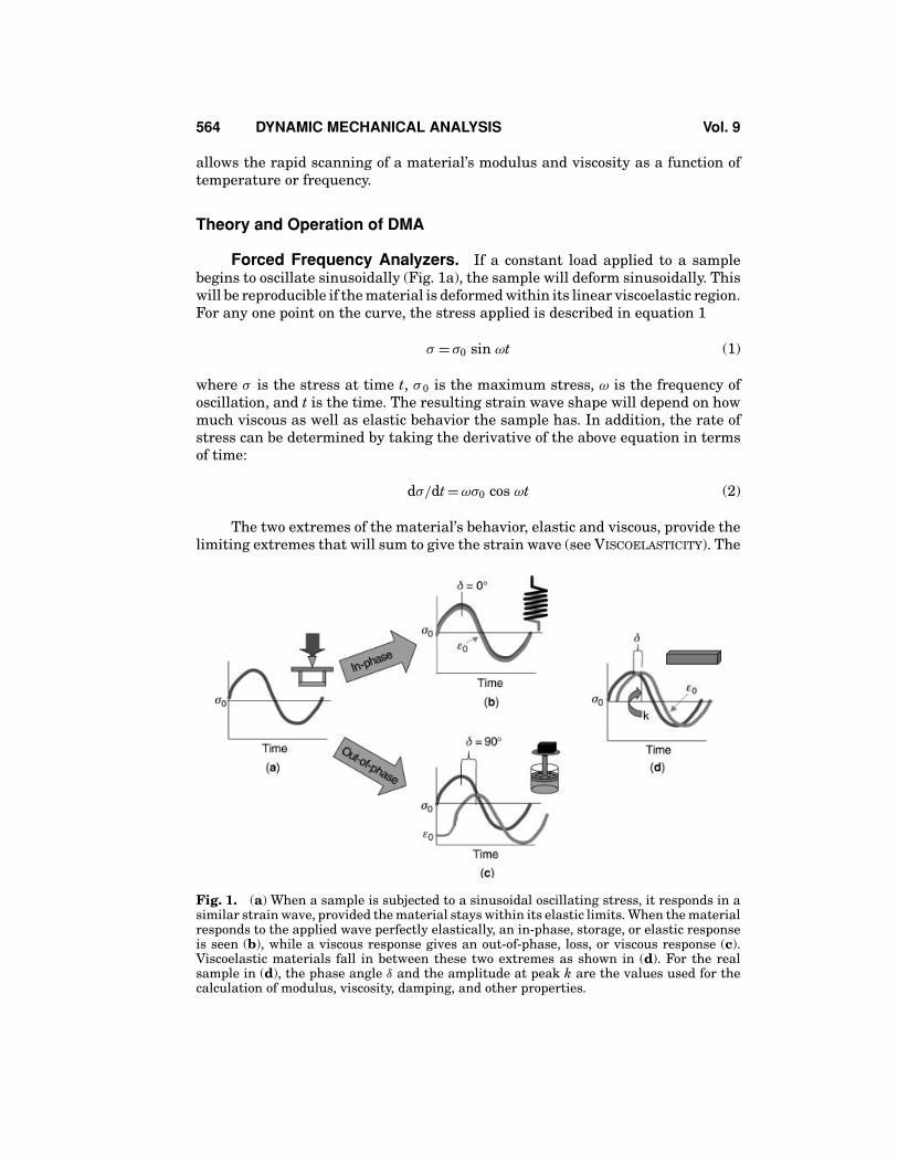
Forced Frequency Analyzers. If a constant load applied to a samplebegins to oscillate sinusoidally (Fig. 1a), the sample will deform sinusoidally. Thiswill be reproducible if the material is deformed within its linear viscoelastic region.For any one point on the curve, the stress applied is described in equation 1

σ = σ0 sin ωt (1)

where σ is the stress at time t, σ 0 is the maximum stress, ω is the frequency ofoscillation, and t is the time. The resulting strain wave shape will depend on howmuch viscous as well as elastic behavior the sample has. In addition, the rate ofstress can be determined by taking the derivative of the above equation in termsof time:

dσ/dt = ωσ0 cos ωt (2)

The two extremes of the material’s behavior, elastic and viscous, provide thelimiting extremes that will sum to give the strain wave (see VISCOELASTICITY). The

Fig. 1. (a) When a sample is subjected to a sinusoidal oscillating stress, it responds in asimilar strain wave, provided the material stays within its elastic limits. When the materialresponds to the applied wave perfectly elastically, an in-phase, storage, or elastic responseis seen (b), while a viscous response gives an out-of-phase, loss, or viscous response (c).Viscoelastic materials fall in between these two extremes as shown in (d). For the realsample in (d), the phase angle δ and the amplitude at peak k are the values used for thecalculation of modulus, viscosity, damping, and other properties.


behavior can be understood by evaluating each of the two extremes. The materialat the spring-like or Hookean limit will respond elastically with the oscillatingstress. The strain at any time can be written as

ε(t) = Eσ0 sin(ωt) (3)

where ε(t) is the strain at any time t, E is the modulus, σ 0 is the maximum stressat the peak of the sine wave, and ω is the frequency. Since in the linear region σ

and ε are linearly related by E, the relationship is

ε(t) = ε0 sin(ωt) (4)

where ε0 is the strain at the maximum stress. This curve shown in Figure 1b hasno phase lag (or no time difference from the stress curve) and is called the in-phaseportion of the curve.

The viscous limit was expressed as the stress being proportional to the strainrate, which is the first derivative of the strain. This is best modeled by a dashpot,and for that element, the term for the viscous response in terms of strain rate isdescribed as

ε(t) = η dσ0/dt = ηωσ0 cos(ωt) (5)

or

ε(t) = ηωσ0 sin(ωt + π/2) (6)

where the terms are as above and η is the viscosity. Substituting terms as abovemakes the equation

ε(t) = ωσ0 cos(ωt) = ωσ0 sin(ωt + π/2) (7)

This curve is shown in Figure 1c. Now, take the behavior of the material thatlies between these two limits. The difference between the applied stress and theresultant strain is an angle δ, and this must be added to equations. So the elasticresponse at any time can now be written as

ε(t) = ε0 sin(ωt + δ) (8)

Using trigonometry this can be rewritten as

ε(t) = ε0[sin(ωt)cos δ + cos(ωt) sin δ] (9)

This equation, corresponding to the curve in Figure 1d, can be separatedinto the in-phase and out-of-phase strains that correspond to curves like those in


Figure1b and 1c, respectively. These are the in-phase and out-phase moduli andare

ε′ = ε0 sin(δ) (10)

ε′′ = ε0 cos(δ) (11)

and the vector sum of these two components gives the overall or complex strainon the sample:

ε∗ = ε′′ + iε′′ (12)

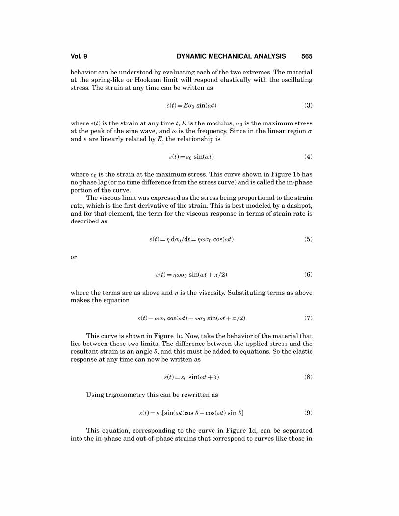
Free Resonance Analyzers. If a suspended sample is allowed to swingfreely, it will oscillate like a harp string as the oscillations gradually come toa stop. The naturally occurring damping of the material controls the decay ofthe oscillations. This produces a wave, shown in Figure 2, which is a series ofsine waves decreasing in amplitude and frequency. Several methods exist to ana-lyze these waves and are covered in the review by Gillham (2,3). These methodshave also been successfully applied to the recovery portion of a creep-recoverycurve where the sample goes into free resonance on removal of the creep force (4).From the decay curve, the period T and the logarithmic decrement � can be cal-culated. Both manual and digital processing methods have been reported (2,3,5).Fuller details of the following may be found in References 2,3, and 5. The decayof the amplitude is evaluated over as many swings as possible to reduce errorReferences:

� = 1/j ln(An/An + j) (13)

Fig. 2. The decay wave from a free resonance analyzer shows the decreasing amplitudeof signal with time. Reprinted with permission from Ref. 1. Copyright (1999) CRC Press.


where j is the number of swings and An is the amplitude of the nth swing. For oneswing, where j = 1, the equation becomes

� = ln(An/An + j) (14)

For a low value of � where An/An+1 is approximately 1, the equation can berewritten as

� ≈ 12

{(A2

n − A2n + 1

)/A2

n

}(15)

From this, since the square of the amplitude is proportional to the storedenergy �W/Wst and the stored energy can be expressed as 2π tan δ, the equationbecomes

� ≈ 12 (�W/Wst) = π tan δ (16)

which gives us the phase angle δ. The time of the oscillations, the period T, canbe found using the following equation:

T = 2π

√M�1

√1 + �

4π2

2

(17)

where �1 is the torque for one cycle and M is the moment of inertia around thecentral axis. Alternatively, T can be calculated directly from the plotted decaycurve as

T = (2/n)(tn − t0) (18)

where n is the number of cycles and t is time. From this, the shear modulus G canbe calculated, which for a rod of length L and radius r is

G =(

4π2MLNT2

)(1 + �2

4π2

)−

(mgr12N

)(19)

where m is the mass of the sample, g the gravitational constant, and N is a geo-metric factor. In the same system, the storage modulus G′ can be calculated as

G′ = (I/T2)(8πML/r4) (20)

where I is the moment of inertia for the system. Having the storage modulusand the tangent of the phase angle, the remaining dynamic properties can becalculated.

Free resonance analyzers normally are limited to rod or rectangular samplesor materials that can be impregnated onto a braid. This last approach is how thecuring studies on epoxy and other resin systems were done in torsion and givesthese instruments the name of torsional braid analyzers (TBA).


Instrumentation. One of the biggest choices made in selecting a DMAis to decide whether to choose stress (force) or strain (displacement) control forapplying the deforming load to the sample. Strain-controlled analyzers, whetherfor simple static testing or for DMA, move the probe a set distance and use a forcebalance transducer or load cell to measure the stress. These parts are typicallylocated on different shafts. The simplest version of this is a screw-driven tester,where the sample is pulled one turn. This requires very large motors so thatthe available force always exceeds what is needed. They normally have bettershort-time response for low viscosity materials and can normally perform stressrelaxation experiments easily. They also usually can measure normal forces if theyare arranged in torsion. A major disadvantage is their transducers may drift atlong times or with low signals.

Stress-controlled analyzers are cheaper to make because there is only oneshaft, but somewhat trickier to use. Many of the difficulties have been allevi-ated by software and many strain-controlled analyzers on the market are reallystress-controlled instruments with feedback loops making them act as if theywere strain-controlled. In stress control, a set force is applied to the sample. Astemperature, time, or frequency varies, the applied force remains the same. Thismay or may not be the same stress: in extension for example, the stretching andnecking of a sample will change the applied stress seen during the run. How-ever, this constant stress is a more natural situation in many cases and it maybe more sensitive to material changes. Good low force control means they are lesslikely to destroy any structure in the sample. Long relaxation times or long creepstudies are more easily performed on these instruments. Their biggest disadvan-tage is that their short-time responses are limited by inertia with low viscositysamples.

Since most DMA experiments are run at very low strains (∼0.5% maximum)to stay well within a polymer’s linear region, it has been reported that both theanalyzers give the same results. However, when one gets to the nonlinear region,the difference becomes significant, as stress and strain are no longer linearlyrelated. Stress control can be said to duplicate real-life conditions more accuratelysince most applications of polymers involve resisting a load.

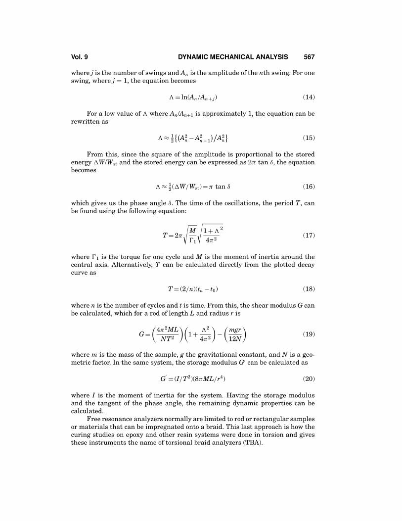
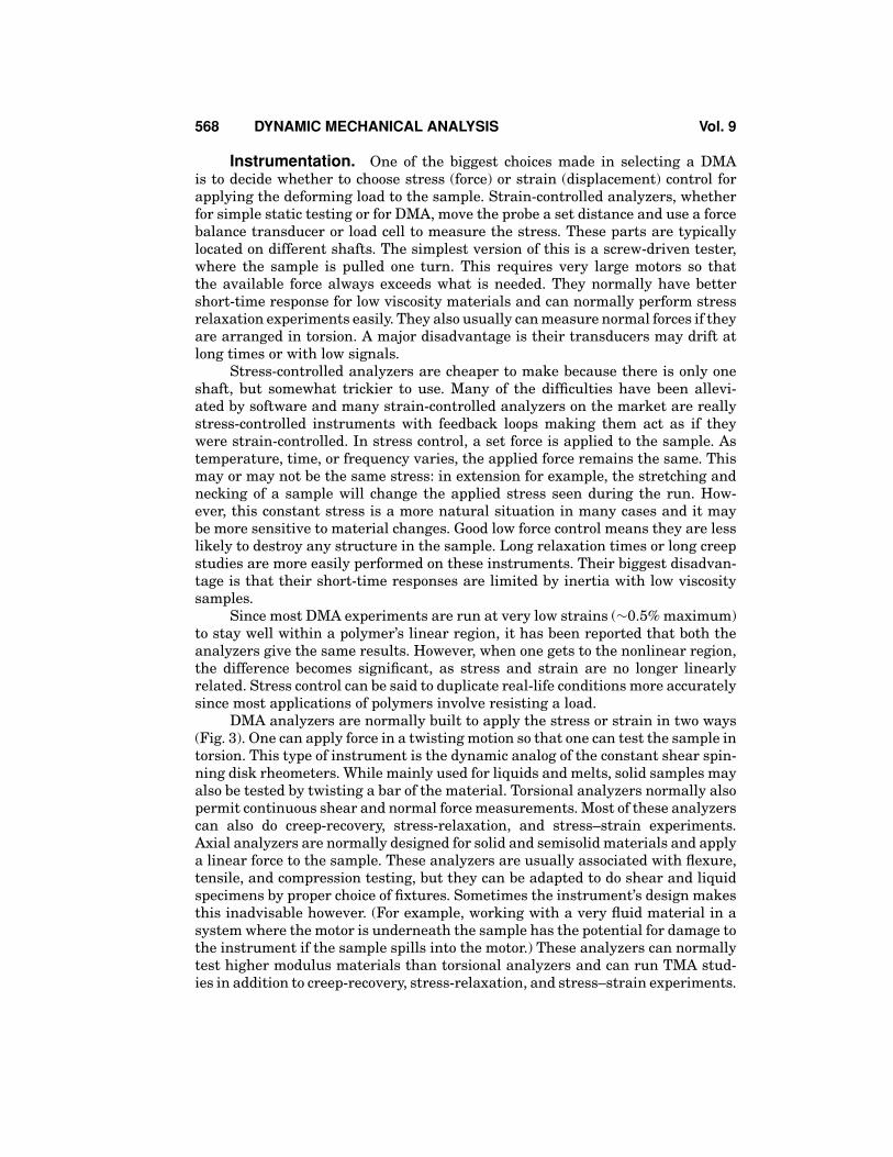
DMA analyzers are normally built to apply the stress or strain in two ways(Fig. 3). One can apply force in a twisting motion so that one can test the sample intorsion. This type of instrument is the dynamic analog of the constant shear spin-ning disk rheometers. While mainly used for liquids and melts, solid samples mayalso be tested by twisting a bar of the material. Torsional analyzers normally alsopermit continuous shear and normal force measurements. Most of these analyzerscan also do creep-recovery, stress-relaxation, and stress–strain experiments.Axial analyzers are normally designed for solid and semisolid materials and applya linear force to the sample. These analyzers are usually associated with flexure,tensile, and compression testing, but they can be adapted to do shear and liquidspecimens by proper choice of fixtures. Sometimes the instrument’s design makesthis inadvisable however. (For example, working with a very fluid material in asystem where the motor is underneath the sample has the potential for damage tothe instrument if the sample spills into the motor.) These analyzers can normallytest higher modulus materials than torsional analyzers and can run TMA stud-ies in addition to creep-recovery, stress-relaxation, and stress–strain experiments.


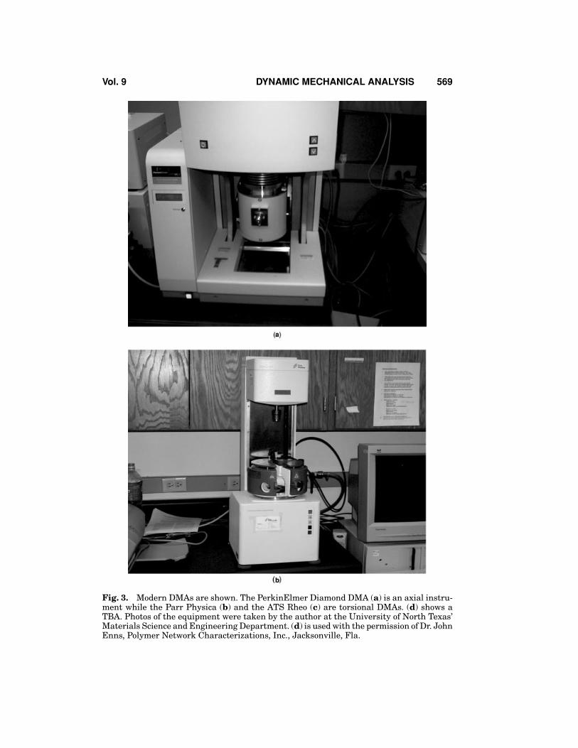
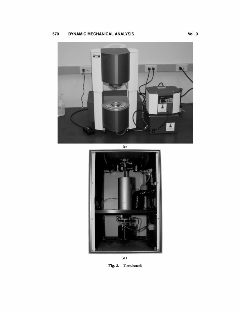
Fig. 3. Modern DMAs are shown. The PerkinElmer Diamond DMA (a) is an axial instru-ment while the Parr Physica (b) and the ATS Rheo (c) are torsional DMAs. (d) shows aTBA. Photos of the equipment were taken by the author at the University of North Texas’Materials Science and Engineering Department. (d) is used with the permission of Dr. JohnEnns, Polymer Network Characterizations, Inc., Jacksonville, Fla.


Fig. 3. (Continued)


There is considerable overlap between the type of samples run by axial and tor-sional instruments. With the proper choice of sample geometry and good fixtures,both types can handle similar samples, as shown by the extensive use of bothtypes to study the curing of neat resins. Normally, axial analyzers cannot handlefluid samples below about 500 Pa · s.

Applications for Thermoplastic Solids and Cured Thermosets

As mentioned above, the thermal transitions in polymers can be described interms of either free volume changes (6) or relaxation times. A simple approachto looking at free volume, which is popular in explaining DMA responses, is thecrankshaft mechanism, where the molecule is imagined as a series of jointedsegments. From this model, it is possible to simply describe the various transitionsseen in a polymer. Other models exist that allow for more precision in describingbehavior; the best seems to be the Doi–Edwards model (7). Aklonis and Knight (8)give a good summary of the available models, as does Rohn (9).

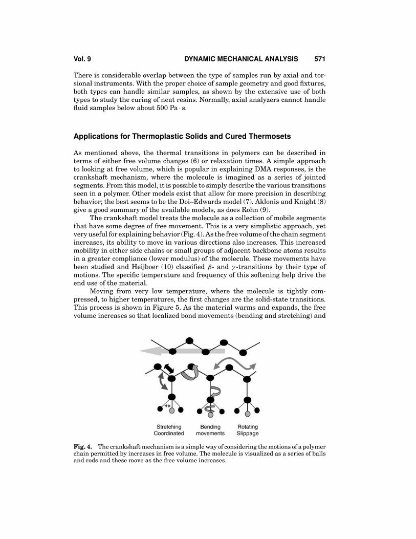
The crankshaft model treats the molecule as a collection of mobile segmentsthat have some degree of free movement. This is a very simplistic approach, yetvery useful for explaining behavior (Fig. 4). As the free volume of the chain segmentincreases, its ability to move in various directions also increases. This increasedmobility in either side chains or small groups of adjacent backbone atoms resultsin a greater compliance (lower modulus) of the molecule. These movements havebeen studied and Heijboer (10) classified β- and γ -transitions by their type ofmotions. The specific temperature and frequency of this softening help drive theend use of the material.

Moving from very low temperature, where the molecule is tightly com-pressed, to higher temperatures, the first changes are the solid-state transitions.This process is shown in Figure 5. As the material warms and expands, the freevolume increases so that localized bond movements (bending and stretching) and

Fig. 4. The crankshaft mechanism is a simple way of considering the motions of a polymerchain permitted by increases in free volume. The molecule is visualized as a series of ballsand rods and these move as the free volume increases.


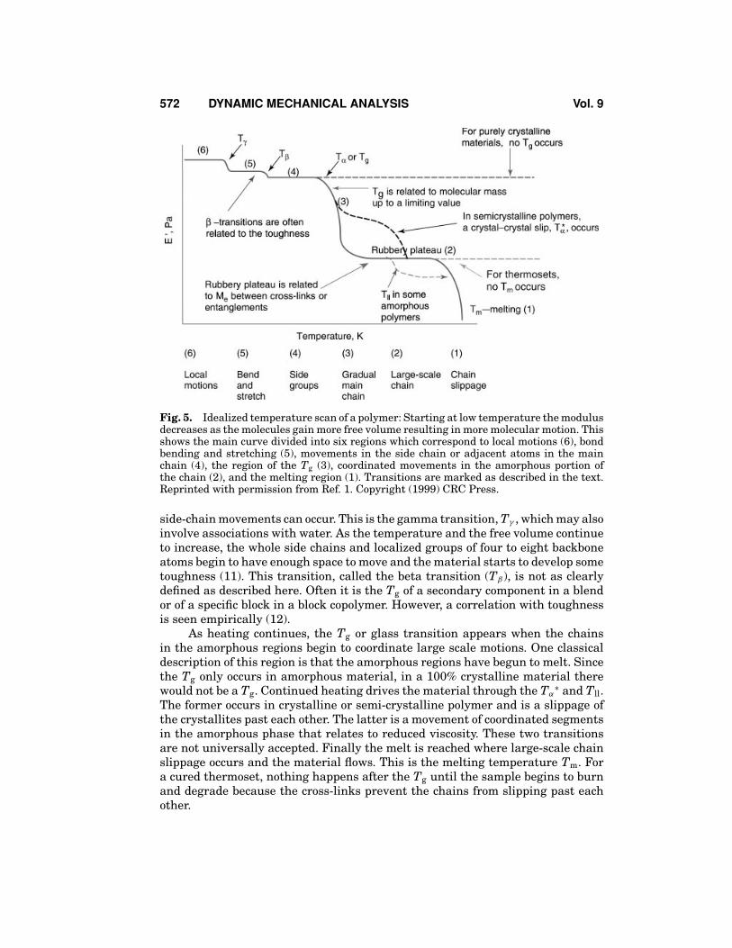
Fig. 5. Idealized temperature scan of a polymer: Starting at low temperature the modulusdecreases as the molecules gain more free volume resulting in more molecular motion. Thisshows the main curve divided into six regions which correspond to local motions (6), bondbending and stretching (5), movements in the side chain or adjacent atoms in the mainchain (4), the region of the Tg (3), coordinated movements in the amorphous portion ofthe chain (2), and the melting region (1). Transitions are marked as described in the text.Reprinted with permission from Ref. 1. Copyright (1999) CRC Press.

side-chain movements can occur. This is the gamma transition, Tγ , which may alsoinvolve associations with water. As the temperature and the free volume continueto increase, the whole side chains and localized groups of four to eight backboneatoms begin to have enough space to move and the material starts to develop sometoughness (11). This transition, called the beta transition (Tβ), is not as clearlydefined as described here. Often it is the Tg of a secondary component in a blendor of a specific block in a block copolymer. However, a correlation with toughnessis seen empirically (12).

As heating continues, the Tg or glass transition appears when the chainsin the amorphous regions begin to coordinate large scale motions. One classicaldescription of this region is that the amorphous regions have begun to melt. Sincethe Tg only occurs in amorphous material, in a 100% crystalline material therewould not be a Tg. Continued heating drives the material through the Tα

∗ and Tll.The former occurs in crystalline or semi-crystalline polymer and is a slippage ofthe crystallites past each other. The latter is a movement of coordinated segmentsin the amorphous phase that relates to reduced viscosity. These two transitionsare not universally accepted. Finally the melt is reached where large-scale chainslippage occurs and the material flows. This is the melting temperature Tm. Fora cured thermoset, nothing happens after the Tg until the sample begins to burnand degrade because the cross-links prevent the chains from slipping past eachother.


This quick overview provides an idea of how an idealized polymer responds.Now a more detailed description of these transitions can be provided with someexamples of their applications. The best general collection of this information isstill McCrum’s 1967 text.

Sub T g Transitions. The area of sub-Tg or higher order transitions hasbeen heavily studied (10,13–19) as these transitions have been associated with me-chanical properties. These transitions can sometimes be seen by DSC and TMA,but they are normally too weak or too broad for determination by these methods.DMA, DEA (dielectric analysis), and similar techniques are usually required (20).Some authors have also called these types of transitions (9,10) second order tran-sitions to differentiate them from the primary transitions of Tm and Tg, whichinvolve large sections of the main chains. Boyer reviewed the Tβ in 1968 (11) andpointed out that while a correlation often exists, the Tβ is not always an indicatorof toughness. Bershtein (21) has reported that this transition can be considered the“activation barrier” for solid-phase reactions, deformation, flow or creep, acousticdamping, physical aging changes, and gas diffusion into polymers as the activationenergies for the transition and these processes are usually similar. The strengthof these transitions is related to how strongly a polymer responses to those pro-cesses. These sub-Tg transitions are associated with the materials properties inthe glassy state. In paints, for example, peel strength (adhesion) can be estimatedfrom the strength and frequency dependence of the sub-ambient beta transition(22). For example, nylon-6,6 shows a decreasing toughness, measured as impactresistance, with declining area under the Tβ peak in the tan δ curve. It has beenshown, particularly in cured thermosets, that increased freedom of movement inside chains increases the strength of the transition. Cheng (15) reports in rigid rodpolyimides that the beta transition is caused by the non-coordinated movement ofthe diamine groups although the link to physical properties was not investigated.Johari has reported in both mechanical (14) and dielectric studies (13) that boththe β- and γ -transitions in bisphenol A based thermosets depend on the side chainsand unreacted ends, and that both are affected by physical aging and postcure.Nelson (23) has reported that these transitions can be related to vibration damp-ing. This is also true for acoustical damping (24). In both of this cases, the strengthof the beta transition is taken as a measurement of how effectively a polymer willabsorb vibrations. There is a frequency dependence in this transitions and this isdiscussed below.

Heijober (10) and Boyer (11) showed that this information needs to be con-sidered with care as not all beta transitions correlate with toughness or otherproperties. This can be due to misidentification of the transition or that the tran-sition does sufficiently disperse energy. A working rule of thumb (10,16,25,26) isthat the beta transition must be related to either localized movement in the mainchain or very large side chain movement to sufficiently absorb enough energy.The relationship of large side chain movement and toughness has been exten-sively studied in polycarbonate by Yee (27) as well as in many other tough glassypolymers (28).

Less use is made of the Tγ transitions and they are mainly studied to un-derstand the movements occurring in polymers. Wendorff (29) reports that thistransition in polyarylates is limited to inter- and intramolecular motions withinthe scale of a single repeat unit. Both McCrum (5) and Boyd (18) similarly limited


the Tγ and Tδ to very small motions either within the molecule or with boundwater. The use of what is called two-dimensional IR, which couples at FTIR anda DMA to study these motions, is a topic of current interest (30,31).

The Glass Transition (T g or T α). As the free volume continues to in-crease with increasing temperature, the glass transition Tg occurs where largesegments of the chain start moving. This transition is also called the α- transi-tion, Tα. The Tg is very dependent on the degree of polymerization up to a valueknown as the critical Tg or the critical molecular weight. Above this value, theTg typically becomes independent of molecular weight (32). The Tg representsa major transition for many polymers, as physical properties change drasticallyas the material goes from a hard glassy to a rubbery state. It defines one endof the temperature range over which the polymer can be used, often called theoperating range of the polymer. For where strength and stiffness are needed, itis normally the upper limit for use. In rubbers and some semicrystalline mate-rials like polyethylene and polypropylene, it is the lower operating temperature.Changes in the temperature of the Tg are commonly used to monitor changes inthe polymer such as plasticizing by environmental solvents and increased cross-linking from thermal or UV aging (see GLASS TRANSITION).

The Tg of cured materials or thin coatings is often difficult to measure byother methods, and more often than not the initial cost justification for a DMA ismeasuring a hard-to-find Tg. While estimates of the relative sensitivity of DMA toDSC or DTA (differential thermal analysis) vary, it appears that DMA is 10–100times more sensitive to the changes occurring at the Tg. The Tg in highly cross-linked materials can easily be seen long after the Tg has become too flat and broadto be seen in DSC. This is also a problem with certain materials like medical gradeurethanes and very highly crystalline polyethylenes.

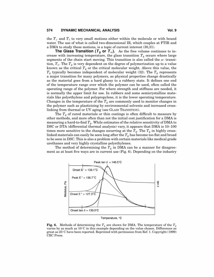
The method of determining the Tg in DMA can be a manner for disagree-ment as at least five ways are in current use (Fig. 6). Depending on the industry

Fig. 6. Methods of determining the Tg are shown for DMA. The temperature of the Tgvaries by as much as 10◦C in this example depending on the value chosen. Differences asgreat as 25◦C have been reported. Reprinted with permission from Ref. 1. Copyright (1999)CRC Press.


standards or background of the operator, the peak or onset of the tan δ curve,the onset of the E′ drop, or the onset or peak of the E′′ curve may be used. Thevalues obtained from these methods can differ up to 25◦C from each other on thesame run. In addition, a 10–20◦C difference from the DSC is also seen in manymaterials. In practice, it is important to specify exactly how the Tg should be de-termined. For DMA, this means defining the heating rate, applied stresses (orstrains), the frequency used, and the method of determining the Tg. For example,the sample will be run at 10◦C◦ min− 1 under 0.05% strain at 1 Hz in nitrogenpurge (20 cc · min− 1) and the Tg determined from the peak of the tan δ curve.

It is not unusual to see a peak or hump on the storage modulus directlypreceding the drop that corresponds to the Tg. This is also seen in DSC and DTAand corresponds to a rearrangement in the material to relieve stresses frozen inbelow the Tg by the processing method. These stresses are trapped in the materialuntil enough mobility is obtained at the Tg to allow the chains to move to a lowerenergy state. Often a material will be annealed by heating it above the Tg and thenslowly cooling it to remove this effect. For similar reasons, some experimenterswill run a material twice or use a heat–cool–heat cycle to eliminate processingeffects.

The Rubbery Plateau, T α∗ and T ll. The area above the Tg and below the

melt is known as the rubbery plateau and its length as well as viscosity are depen-dent on the molecular weight between entanglements (Me) (33) or cross-links. Themolecular weight between entanglements is normally calculated during a stress-relaxation experiment but similar behavior is observed in DMA. The modulus inthe plateau region is proportional to either the number of cross-links or the chainlength between entanglements. This is often expressed in shear as

G′ ∼= (ρRT)/Me (21)

where G′ is the shear storage modulus of the plateau region at a specific tempera-ture, ρ is the polymer density, and Me is the molecular weight between entangle-ments. In practice, the relative modulus of the plateau region shows the relativechanges in Me or the number of cross-links compared to a standard material.

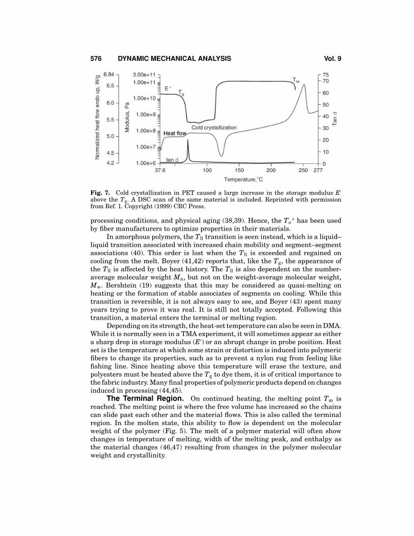
The rubbery plateau is also related to the degree of crystallinity in a material,although DSC is a better method for characterizing crystallinity than DMA (34,35). Also as in the DSC, there is evidence of cold crystallization in the temperaturerange above the Tg (Fig. 7). That is one of several transitions that can be seen inthe rubbery plateau region. This crystallization occurs when the polymer chainshave been quenched (quickly cooled) into a highly disordered state. On heatingabove the Tg, these chains gain enough mobility to rearrange into crystallites,which causes a sometimes-dramatic increase in modulus. DSC or its temperature-modulated variant, StepScanTM Differential Scanning Calorimetry, can be usedto confirm this (36). The alpha star transition Tα

∗, the liquid–liquid transitionTll, the heat-set temperature, and the cold crystallization peak are all transitionsthat can appear on the rubbery plateau. In some crystalline and semicrystallinepolymer, a transition is seen here called the Tα

∗ (18,37). The alpha star transitionis associated with the slippage between crystallites and helps extend the operatingrange of a material above the Tg. This transition is very susceptible to processinginduced changes and can be enlarged or decreased by the applied heat history,


Fig. 7. Cold crystallization in PET caused a large increase in the storage modulus E′

above the Tg. A DSC scan of the same material is included. Reprinted with permissionfrom Ref. 1. Copyright (1999) CRC Press.

processing conditions, and physical aging (38,39). Hence, the Tα∗ has been used

by fiber manufacturers to optimize properties in their materials.In amorphous polymers, the Tll transition is seen instead, which is a liquid–

liquid transition associated with increased chain mobility and segment–segmentassociations (40). This order is lost when the Tll is exceeded and regained oncooling from the melt. Boyer (41,42) reports that, like the Tg, the appearance ofthe Tll is affected by the heat history. The Tll is also dependent on the number-average molecular weight Mn, but not on the weight-average molecular weight,Mw. Bershtein (19) suggests that this may be considered as quasi-melting onheating or the formation of stable associates of segments on cooling. While thistransition is reversible, it is not always easy to see, and Boyer (43) spent manyyears trying to prove it was real. It is still not totally accepted. Following thistransition, a material enters the terminal or melting region.

Depending on its strength, the heat-set temperature can also be seen in DMA.While it is normally seen in a TMA experiment, it will sometimes appear as eithera sharp drop in storage modulus (E′) or an abrupt change in probe position. Heatset is the temperature at which some strain or distortion is induced into polymericfibers to change its properties, such as to prevent a nylon rug from feeling likefishing line. Since heating above this temperature will erase the texture, andpolyesters must be heated above the Tg to dye them, it is of critical importance tothe fabric industry. Many final properties of polymeric products depend on changesinduced in processing (44,45).

The Terminal Region. On continued heating, the melting point Tm isreached. The melting point is where the free volume has increased so the chainscan slide past each other and the material flows. This is also called the terminalregion. In the molten state, this ability to flow is dependent on the molecularweight of the polymer (Fig. 5). The melt of a polymer material will often showchanges in temperature of melting, width of the melting peak, and enthalpy asthe material changes (46,47) resulting from changes in the polymer molecularweight and crystallinity.


Degradation, polymer structure, and environmental effects all influencewhat changes occur. Polymers that degrade by cross-linking will look very dif-ferent from those that exhibit chain scission. Very highly cross-linked polymerswill not melt as they are unable to flow.

The study of polymer melts and especially their elasticity was one of theareas that drove the development of commercial DMAs. Although a decrease inthe melt viscosity is seen with temperature increases, the DMA is most commonlyused to measure the frequency dependence of the molten polymer as well as itselasticity. The latter property, especially when expressed as the normal forces, isvery important in polymer processing.

Frequency Dependencies in Transition Studies. The choice of a test-ing frequency or its effect on the resulting data must be addressed. A short dis-cussion of how frequencies are chosen and how they affect the measurement oftransitions is in order. Considering that higher frequencies induce more elastic-like behavior, there is some concern that a material will act stiffer than it really isif the test frequency is chosen to be too high. Frequencies for testing are normallychosen by one of three methods. The most scientific method would be to use thefrequency of the stress or strain that the material is exposed to in the real world.However, this is often outside of the range of the available instrumentation. Insome cases, the test method or the industry standard sets a certain frequency andthis frequency is used. Ideally a standard method like this is chosen so that thedata collected on various commercial instruments can be shown to be compatible.Some of the ASTM methods for TMA (thermomechanical analysis) and DMA arelisted in Table 1. Many industries have their own standards so it is important to

Table 1. ASTM test for DMA

D3386 CTE of electrical insulating materials by TMAD4065 Determining DMA properties terminologya

D4092 Terminology for DMA testsD4440 Measurement of polymer meltsD4473 Cure of thermosetting resinsD5023 DMA in three-point bending testsD5024 DMA in compressionD5026 DMA in tensionD5279 DMA of plastics in tensionD5418 DMA in dual cantileverD5934 DMA tensile modulus under constant loadingD6382 DMA testing on waterproof roffing materialsD228-95 CTE by TMA with silica dilatometerE473-94 Terminology for thermal analyusisE831-93 CTE of solids by TMAE1363-97 Temperature calibration for TMAE1545-95(a) Tg by TMAE1640-99 Tg by DMAE1824-96 Tg by TMA in tensionE1867-01 Temperature calibration for DMAE2254-03 Storage moldulus calibration for DMAaThis standard qualifies a DMA as a acceptable for all ASTM DMAstandards.


know whether the data is expected to match a Mil-spec, an ASTM standard, or aspecific industrial test. Finally, one can arbitrarily pick a frequency. This is donemore often than not, so that 1 Hz and 10 rad · s− 1 are often used. As long as thedata are run under the proper conditions, they can be compared to highlight mate-rial differences. This requires that frequency, stresses, and the thermal programbe the same for all samples in the data set.

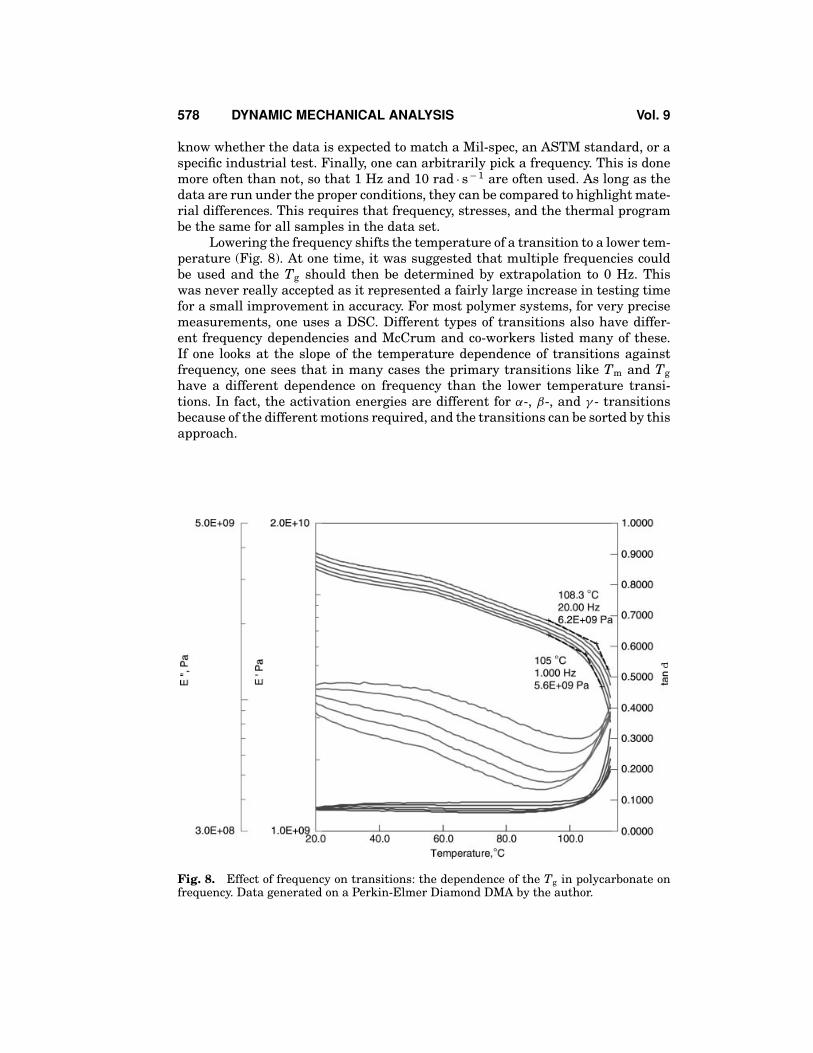
Lowering the frequency shifts the temperature of a transition to a lower tem-perature (Fig. 8). At one time, it was suggested that multiple frequencies couldbe used and the Tg should then be determined by extrapolation to 0 Hz. Thiswas never really accepted as it represented a fairly large increase in testing timefor a small improvement in accuracy. For most polymer systems, for very precisemeasurements, one uses a DSC. Different types of transitions also have differ-ent frequency dependencies and McCrum and co-workers listed many of these.If one looks at the slope of the temperature dependence of transitions againstfrequency, one sees that in many cases the primary transitions like Tm and Tghave a different dependence on frequency than the lower temperature transi-tions. In fact, the activation energies are different for α-, β-, and γ - transitionsbecause of the different motions required, and the transitions can be sorted by thisapproach.

Fig. 8. Effect of frequency on transitions: the dependence of the Tg in polycarbonate onfrequency. Data generated on a Perkin-Elmer Diamond DMA by the author.


Polymer Melts and Solutions, Applications

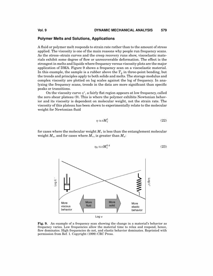
A fluid or polymer melt responds to strain rate rather than to the amount of stressapplied. The viscosity is one of the main reasons why people run frequency scans.As the stress–strain curves and the creep recovery runs show, viscoelastic mate-rials exhibit some degree of flow or unrecoverable deformation. The effect is thestrongest in melts and liquids where frequency versus viscosity plots are the majorapplication of DMA. Figure 9 shows a frequency scan on a viscoelastic material.In this example, the sample is a rubber above the Tg in three-point bending, butthe trends and principles apply to both solids and melts. The storage modulus andcomplex viscosity are plotted on log scales against the log of frequency. In ana-lyzing the frequency scans, trends in the data are more significant than specificpeaks or transitions.

On the viscosity curve η∗, a fairly flat region appears at low frequency, calledthe zero shear plateau (9). This is where the polymer exhibits Newtonian behav-ior and its viscosity is dependent on molecular weight, not the strain rate. Theviscosity of this plateau has been shown to experimentally relate to the molecularweight for Newtonian fluid

η ∝ cM1v (22)

for cases where the molecular weight Mv is less than the entanglement molecularweight Me, and for cases where Mv, is greater than Me:

η0 ∝ cM3.4v (23)

Fig. 9. An example of a frequency scan showing the change in a material’s behavior asfrequency varies. Low frequencies allow the material time to relax and respond, hence,flow dominates. High frequencies do not, and elastic behavior dominates. Reprinted withpermission from Ref. 1. Copyright (1999) CRC Press.


where η0 is the viscosity of the initial Newtonian plateau, c is a material con-stant, and Mv the viscosity average molecular weight. This relationship can bewritten in general terms, replacing the exponential term with the Mark-Houwinkconstant a. Equation 23 can be used as a method of approximating the molecularweight of a polymer. The value obtained is closest to the viscosity-average molec-ular weight obtained by osmometry (48). In comparison with the weight-averagedata obtained by gel permeation chromatography, the viscosity-average molecu-lar weight would be between the number-average and weight-average molecularweights, but closer to the latter (49). This was originally developed for steadyshear viscosity but applies to complex viscosity as well. The relationship betweensteady shear and complex viscosity is fairly well established. Cox and Merz (50)found that an empirical relationship exists between complex viscosity and steadyshear viscosity when the shear rates are the same. The Cox–Merz rule is statedbelow:

|η(ω)| = η(γ̇ )|γ̇ = ω (24)

where η is the constant shear viscosity, η∗ is the complex viscosity, ω the frequencyof the dynamic test, and dγ /dt the shear rate of the constant shear test. This rule ofthumb seems to hold for most materials to within about ±10%. Another approachis the Gleissile (51) Mirror Relationship that states the following:

ηγ̇ = η+ (t)|t = 1/γ̇ (25)

when η+(t) is the limiting value of the viscosity as the shear rate γ̇ approacheszero.

The low frequency range is where viscous or liquid-like behavior predomi-nates. If a material is stressed over long enough times, some flow occurs. As timeis the inverse of frequency, this means materials are expected to flow more at lowfrequency. As the frequency increases, the material will act in a more and moreelastic fashion. Silly Putty (Billy and Smith, Inc.), the children’s toy, shows thisclearly. At low frequency, Silly Putty flows like a liquid, while at high frequency itbounces like a rubber ball. This behavior is also similar to what happens with tem-perature changes. A polymer becomes softer and more fluid as it is heated and itgoes through transitions that increase the available space for molecular motions.Over long enough time periods, or small enough frequencies, similar changes oc-cur. So one can move a polymer across a transition by changing the frequency. Thisrelationship is also expressed as the idea of time–temperature equivalence (52).Often stated, as low temperature is equivalent to short times or high frequency,it is a fundamental rule of thumb in understanding polymer behavior.

As the frequency is increased in a frequency scan, the Newtonian regionis exceeded and a new relationship develops between the rate of strain, or thefrequency, and the viscosity of the material. This region is often called the powerlaw zone and can be modeled by

η∗ ∼= η(γ̇ ) = cγ̇ n − 1 (26)


where η∗ is the complex viscosity, γ̇ is the shear rate, and the exponent term n isdetermined by the fit of the data. This can also be written as

σ ∼= η(γ̇ ) = cγ̇ n (27)

where σ is the stress and η is the viscosity. The exponential relationship is whythe viscosity versus frequency plot is traditionally plotted on a log scale. Withmodern curve fitting programs, the use of log–log plots has declined and is abit anachronistic. The power law region of polymers shows shear thickening orthinning behavior. This is also the region in which the E′–η∗ or the E′–E′′ crossoverpoint is found. As frequency increases and shear thinning occurs, the viscosity (η∗)decreases. At the same time, increasing the frequency increases the elasticity (E′).This is shown in Figure 9. The E′–η∗ crossover point is used an indicator of themolecular weight and molecular weight distribution (53). Changes in its positionare used as a quick method of detecting changes in the molecular weight anddistribution of a material. After the power law region, another plateau is seen,the infinite shear plateau.

This second Newtonian region corresponds to where the shear rate is so highthat the polymer no longer shows a response to increases in the shear rate. At thevery high shear rates associated with this region, the polymer chains are no longerentangled. This region is seldom seen in DMA experiments and usually avoidedin use because of the damage done to the chains. It can be reached in commercialextruders and can cause degradation of the polymer, which causes the poorerproperties associated with regrind.

As the curve in Figure 9 shows, the modulus also varies as a function of thefrequency. A material exhibits more elastic-like behavior as the testing frequencyincreases, and the storage modulus tends to slope upwards toward higher fre-quency. The storage modulus’ change with frequency depends on the transitionsinvolved. Above the Tg, the storage modulus tends to be fairly flat, with a slight in-crease with increasing frequency as it is on the rubbery plateau. The change in theregion of a transition is greater. If one can generate a modulus scan over a wideenough frequency range, the plot of storage modulus versus frequency appearslike the reverse of a temperature scan. The same time–temperature equivalencediscussed above also applies to modulus, as well as compliance, tan δ, and otherproperties.

The frequency scan is used for several purposes that will be discussed in thissection. One very important use, that is very straightforward, is to survey thematerial’s response over various shear rates. This is important because many ma-terials are used under different conditions. For example adhesives, whether tape,Band-Aids, or hot melts, are normally applied under conditions of low frequencyand this property is referred to as tack. When they are removed, the removaloften occurs under conditions of high frequency called peel. Different propertiesare required at these regimes and to optimize one property may require chemicalchanges that harm the other. Similarly, changes in polymer structure can showthese kinds of differences in the frequency scan. For example, branching affectsdifferent frequencies (9).

In a tape adhesive, for example, sufficient flow under pressure at low fre-quency is desired to fill the pores of the material to obtain a good mechanical


bond. When the laminate is later subjected to peel, the material needs to be veryelastic so that it will not pull out of the pores (54,55). The frequency scan allowsmeasurement of these properties in one scan thus ensuring that tuning one prop-erty does not degrade another. This type of testing is not limited to adhesives asmany materials see multiple frequencies in the actual use. Viscosity versus fre-quency plots are used extensively to study how changes in polymer structure orformulations affect the behavior of the melt. Often changes in materials, especiallyin uncured thermosetting resins and molten materials, effect a limited frequencyrange and testing at a specific frequency can miss the problem.

It should be noted that since the material is scanned across a frequencyrange, there are some conditions where the material–instrument system acts likea guitar string and begins to resonate when certain frequencies are reached. Thesefrequencies are either the natural resonance frequency of the sample–instrumentsystem or one of its harmonics. When the harmonics occur, the sample–instrumentsystem oscillates like a guitar string and the desired information about the sampleis obscured. Since there is no way to change this resonance behavior (and in afree resonance analyzer, this effect is necessary to obtain data), it is required toredesign the experiment by changing sample dimensions or geometry to escapethe problem. Using a sample with much different dimensions, which change themass, or changing from extension to three-point bending geometry changes thenatural oscillation frequency of the sample and hopefully solves this problem.

Thermosets, Applications

The DMA’s ability to give viscosity and modulus values for each point in a tem-perature scan allows the estimation of kinetic behavior as a function of viscosity.This has the advantage of describing how viscous the material is at any giventime, so as to determine the best time to apply pressure, what design of tooling touse, and when the material can be removed from the mold. Recent reviews havesummarized this approach for epoxy systems (56).

Curing. The simplest way to analyze a resin system is to run a plain tem-perature ramp from ambient to some elevated temperature (57,58). This “cure pro-file” allows collection of several vital pieces of information as shown in Figure 10.Samples may be run “neat” or impregnated into fabrics in techniques that arereferred to as torsional braid. There are some problems with this technique, astemperature increases will cause an apparent curing of nondrying oils as thermalexpansion increases friction. However, the “soaking of resin into a shoelace,” asthis technique has been called, allows one to handle difficult specimens underconditions where the pure resin is impossible to run in bulk (due to viscosity orevolved volatiles). Composite materials like graphite–epoxy composites are some-times studied in industrial situations as the composite rather than the “neat” orpure resin because of the concern that the kinetics may be significantly different.In terms of ease of handling and sample, the composite is a better sample. Anotherarea of concern is paints and coatings (59) where the material is used in a thinlayer. This can be addressed experimentally by either a braid as above or coatingthe material on a thin sheet of metal. The metal is often run first and its scan


Fig. 10. The DMA cure profile of a two-part epoxy showing the typical analysis for mini-mum viscosity, gel time, vitrification time, and estimation of the action energy (see discus-sion in text). Reprinted with permission from Ref. 1. Copyright (1999) CRC Press.

subtracted from the coated sheet’s scan to leave only the scan of the coating. Thisis also done with thin films and adhesive coatings.

From the cure profile seen in Figure 10, it is possible to determine the mini-mum viscosity (η∗

min), the time to η∗min and the length of time it stays there, the

onset of cure, the point of gelation where the material changes from a viscousliquid to a viscoelastic solid, and the beginning of vitrification. The minimum vis-cosity is seen in the complex viscosity curve and is where the resin viscosity isthe lowest. A given resin’s minimum viscosity is determined by the resin’s chem-istry, the previous heat history of the resin, the rate at which the temperature isincreased, and the amount for stress or strain applied. Increasing the rate of thetemperature ramp is known to decrease the η∗

min, the time to η∗min, and the gel

time. The resin gets softer faster, but also cures faster. The degree of flow limitsthe type of mold design and when as well as how much pressure can be appliedto the sample. The time spent at the minimum viscosity plateau is the result of acompetitive relationship between the material’s softening or melting as it heatsand its rate of curing. At some point, the material begins curing faster than itsoftens, and that is where the viscosity starts to increase.

As the viscosity begins to climb, an inversion is seen of the E′′ and E′ valuesas the material becomes more solid-like. This crossover point also corresponds towhere the tan δ equals 1 (since E′ = E′′ at the crossover). This is taken to be the gelpoint, (60) where the cross-links have progressed to forming an “infinitely” longnetwork across the specimen. At this point, the sample will no longer dissolve insolvent. While the gel point correlates fairly often with this crossover, it doesn’talways. For example, for low initiator levels in chain addition thermosets, thegel point precedes the modulus crossover (61). A temperature dependence for thepresence of the crossover has also been reported (57,58). In some cases, wherepowder compacts and melts before curing, there may be several crossovers (62).


Then, the one following the η∗min is usually the one of interest. Some researchers

(63,64) believe that the true gel point is best detected by measuring the frequencydependence of the crossover point. This is done either by multiple runs at differentfrequencies or by multiplexing frequencies during the cure. At the gel point, thefrequency dependence disappears (64). This value is usually only a few degreesdifferent from the one obtained in a normal scan and in most cases not worth theadditional time. During this rapid climb of viscosity in the cure, the slope for η∗

increase can be used to calculate an estimated Ea (activation energy) (65). Thiswill be discussed below, but the fact that the slope of the curve here is a function ofEa is important. Above the gel temperature, some workers estimate the molecularweight, Mc, between cross-links as

G′ = RTρ/Mc (28)

where R is the gas constant, T is the temperature in Kelvin, and ρ is the density. Atsome point the curve begins to level off and this is often taken as the vitrificationpoint, Tvf.

The vitrification point is where the cure rate slows because the material hasbecome so viscous that the bulk reaction has stopped. At this point, the rate of cureslows significantly. The apparent Tvf however is not always real: any analyzer inthe world has an upper force limit. When that force limit is reached, the “toppingout” of the analyzer can pass as the Tvf. Use of a combined technique like DMA–DEA DEA is dielectric analysis, where an oscillating electrical signal is appliedto a sample. From this signal, the ion mobility can be calculated, which is thenconverted to a viscosity (see Ref. 5 for details). DEA will measure to significantlyhigher viscosities than DMA to see the higher viscosities or the removal of asample from parallel plate and sectioning it into a flexure beam is often necessaryto see the true vitrification point. Vitrification may also be seen in the DSC if amodulated temperature technique like StepScan is used (66). A reaction can alsocompletely cure without vitrifying and will level off the same way. One shouldbe aware that reaching vitrification or complete cure too quickly could be as badas too slowly. Often an overly aggressive cure cycle will cause a weaker materialas it does not allow for as much network development, but gives a series of hard(highly cross-linked) areas among softer (lightly cross-linked) areas. On the way tovitrification, an important value is 106 Pa · s. This is the viscosity of bitumen (67)and is often used as a rule of thumb for where a material is stiff enough to supportits own weight. This is a rather arbitrary point, but is chosen to allow the removalof materials from a mold and the cure is then continued as a post-cure step. Thecure profile is both a good predictor of performance as well as a sensitive probeof processing conditions. As discussed above under TMA applications, a volumechange occurs during the cure (68). This shrinkage of the resin is important andcan be studied by monitoring the probe position of some DMA’s as well as by TMAand dilatometry.

The above is based on using a simple temperature ramp to see how a ma-terial responds to heating. In actual use, many thermosets are actually curedusing more complex cure cycles to optimize the tradeoff between the processing


time and the final product’s properties (69). The use of two-stage cure cyclesis known to develop stronger laminates in the aerospace industry. Exception-ally thick laminates often also require multiple stage cycles in order to developstrength without porosity. As thermosets shrink on curing, careful developmentof a proper cure cycle to prevent or minimize internal voids is necessary. Onereason for the use of multistage cures is to drive reactions to completion. An-other is to extend the minimum viscosity range to allow greater control in form-ing or shaping of the material. The development of a cure cycle with multipleramps and holds would be very expensive if done with full-sized parts in pro-duction facilities. The use of the DMA gives a faster and cheaper way of op-timizing the cure cycle to generate the most efficient and tolerant processingconditions.

Because of the limits of industrial equipment and cost constraints, curingis done at a constant temperature for a period of time. This can be done bothto initially cure the material or to “post-cure” it. (The kinetic models discussedin the next section also require data collected under isothermal conditions.) It isalso how rubber samples are cross-linked, how initiated reactions are run, andhow bulk polymerizations are performed. Industrially, continuous processes, asopposed to batch, often require an isothermal approach. UV light and other formsof nonthermal initiation also use isothermal studies for examining the cure at aconstant temperature.

Photocuring. A photocure in the DMA is run by applying a UV light sourceto a sample (held a specific temperature or subjected to a specific thermal cycle)(70). Photocuring is done for dental resin, contact adhesives, and contact lenses.UV-exposure studies are also run on cured and thermoplastic samples by thesame techniques as photocuring to study UV degradation. The cure profile of aphotocure is very similar to that of a cake or epoxy cement. The same analysisis used and the same types of kinetics developed as is done for thermal curingstudies.

The major practical difficulty in running photocures in the DMA is the cur-rent lack of a commercially available photocuring accessory, comparable to thephotocalorimeters on the market. One normally has to adapt a commercial DMA torun these experiments. The Perkin-Elmer DMA-7e has been successfully adapted(71) to use quartz fixtures and commercial UV source from EFOS, triggered fromthe DMA’s software. This is a fairly easy process and other instruments like theRheoSciTM DMTA (dynamic mechanical thermal analyzer) Mark 5 have also beenadapted.

Curing Kinetics by DMA. Several approaches have been developed tostudying the chemorheology of thermosetting systems. MacKay and Halley (72)reviewed chemorheology and the more common kinetic models. A fundamentalmethod is the Williams–Landel–Ferry (WLF) model, (73) which looks at the vari-ation of Tg with degree of cure. This has been used and modified extensively (74).A common empirical model for curing has been proposed by Roller (75,76). In thelatter approach, samples of the thermoset are run isothermally as described aboveand the viscosity versus time data collected. This is plotted as log (versus time inseconds, where a change in slope is apparent in the curve. This break in the dataindicates the sample is approaching the gel time. From these curves, the initialviscosity, η0 and the apparent kinetic factor k can be determined. By plotting the


log viscosity versus time for each isothermal run, the slope k, and the viscosity att = 0 are apparent. The initial viscosity and k can be expressed ase

η0 = η∞ e�Eη/RT (29)

k = k∞ e�Ek/RT (30)

Combining these allows setup of the equation for viscosity under isothermal con-ditions as

ln η(t) = ln η∞ + �Ek/RT + tk∞e�Ek/RT (31)

By replacing the last term with an expression that treats temperature as afunction of time, the equation becomes

ln η(T, t) = ln η∞ +�Eη/RT +∫ t

0k∞ e�Ek/RT dt (32)

This equation can be used to describe viscosity–time profiles for any runwhere the temperature can be expressed as a function of time. The activation en-ergies can now be calculated. The plots of the natural log of the initial viscosity(determined above) versus 1/T and the natural log of the apparent rate constantk versus 1/T are used to give us the activation energies �Eη and �Ek. Compari-son of these values to the k and �E to those calculated by DSC shows that thismodel gives larger values (59). The DSC data is faster to obtain, but it does notinclude the needed viscosity information. Several corrections have been proposed,addressing different orders of reaction (77) (the above assumes first order) andmodifications to the equations (78,79). Many of these adjustments are reportedin Roller’s 1986 review (76) of curing kinetics. It is noted that these equations donot work well above the gel temperature. This same equation has been used topredict the degradation of properties in thermoplastics successfully (80).

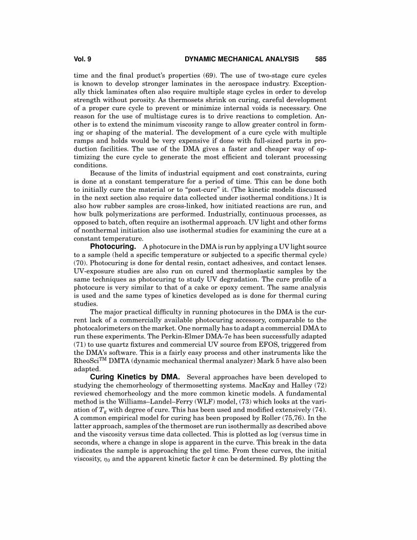
The Gillham–Enns Diagram. The most complete approach to studyingthe behavior of a thermoset was developed by Gillham (81,82) and is analogous tothe phase diagrams used by metallurgists. The time–temperature–transformationdiagram (TTT) or the Gillham–Enns diagram (after its creators) is used to trackthe effects of temperature and time on the physical state of a thermosetting mate-rial. Figure 11 shows an example. Running isothermal studies of a resin at varioustemperatures and recording the changes as a function of time can do this. Onehas to choose values for the various regions and Gillham has done an excellentjob of detailing how one picks the Tg, the glass, the gel, the rubbery, and the char-ring regions (3,83). These diagrams are also generated from DSC data (84), andseveral variants, (85) like the continuous heating transformation and conversion–temperature–property diagrams, have been reported. While easy to develop anduse, TTT diagrams have not yet been accepted in industry despite their obviousutility. This may be due to the fact that they take some time to generate. A recentreview (3) will hopefully increase the use of this approach.


Fig. 11. An example of the Gillham–Enns diagram generated by the author on a com-mercial epoxy resin system. The lines of gelation and vitrification are marked.

BIBLIOGRAPHY

“Dynamic Mechanical Properties” in EPSE 2nd ed., Vol. 5, pp. 299–329, by T. Murayama,Monsanto Co.

1. K. Menard, Dynamic Mechanical Analysis: A Practical Introduction, CRC Press, BocaRaton, Fla., 1999.

2. J. Gillham, in J. Dworkins, ed., Developments in Polymer Characterizations, Vol. 3,Applied Science Publishers, Princeton, N.J., 1982, pp. 159–227.

3. J. Gillham and J. Enns, Trends Polym. Sci. 2, 406 (1994).4. U. Zolzer and H.-F. Eicke, Rheol. Acta 32, 104 (1993).5. N. McCrum, B. E. Read, and G. Williams, Anelastic and Dielectric Properties of Poly-

meric Solids, Dover, New York, 1991, pp. 192–200.6. P. Flory, Principles of Polymer Chemistry, Cornell University Press, Ithaca, N.Y., 1953.7. M. Doi and S. Edwards, The Dynamics of Polymer Chains, Oxford University Press,

New York, 1986.8. J. J. Aklonis and W. J. MacKnight, Introduction to Viscoelasticity, John Wiley & Sons,

Inc., New York, 1983.9. C. L. Rohn, Analytical Polymer Rheology, Hanser-Gardener, New York, 1995.

10. J. Heijboer, Int. J. Polym. Mater. 6, 11 (1977).11. R. F. Boyer, Polym. Eng. Sci. 8(3), 161, (1968).12. Ref. 9, pp. 279–283.13. M. Mangion and G. Johari, J. Polym. Sci., Part B: Polym. Phys. 29, 437 (1991).14. G. Johari and G. Mikoljaczak, J. Cavaille, Polym. 28, 2023 (1987).15. F. Arnold, M. Eashoo, D. Shen, C. Lee, K. Bruno, and S. Cheng, Polym. Sci. Eng. 33,

373 (1993).16. G. Johari, Lect. Notes Phys. 277, 90 (1987).


17. R. Daiz-Calleja and E. Riande, Rheol. Acta 34, 58 (1995).18. R. Boyd, Polym. 26, 323 (1985).19. V. Bershtien, V. Egorov, L. Egorova, and V. Ryzhov, Thermochim. Acta 238, 41 (1994).20. B. Twombly, Proc. NATAS 20, 63 (1991).21. V. Bershtien and V. Egorov, Differential Scanning Calorimetery in the Physical Chem-

istry of Polymers, Ellis Horwood, Chichester, U.K., 1993.22. B. Coxton, private communication, 1996.23. F. C. Nelson, Shock, and Vibration, Digest 26(2), 11 & 24 (1994).24. W. Brostow, private communication, 1998.25. J. Heijboer, in J. Prins, ed., Physics of Non-Crystalline Solids, Wiley-Interscience, New

York, 1965.26. J. Heijboer, J. Polym. Sci., Part C 1 6, 3755 (1968); L. Nielsen and R. Landel, J.

Macromol. Sci., Phys. 9, 239 (1974); S. Wu, J. Appl. Polym. Sci. 46, 619 (1986).27. A. Yee and S. Smith, Macromolecules 14, 54 (1981).28. G. Gordon, J. Polym. Sci., Part A 2, 9, 1693 (1984).29. J. Wendorff and B. Schartel, Polym. 36, 899 (1995).30. I. Noda, Appl. Spectrosc. 44, 550 (1990).31. V. Kien, in Proc. 6th Sympos. Radiation Chem., Vol. 6, Issue 2, 1987, p. 463.32. L. H. Sperling, Introduction to Physical Polym. Science, 2nd ed., John Wiley & Sons,

Inc., New York, 1992.33. C. Macosko, Rheology, VCH Publishers, New York, 1994.34. T. Hatakeyama and F. Quinn, Thermal Analysis, John Wiley & Sons, Inc., New York,

1994.35. B. Wunderlich, Thermal Analysis, Academic Press, New York, 1990.36. J. Schawe, Thermochim. Acta 261, 183 (1995); J. Schawe, Thermochim. Acta 260, 1

(1995); J. Schawe, Thermochim. Acta 271, 1 (1995); B. Wunderlich, A. Boller, and Y.Jin, J. Therm. Anal. 42, 949 (1994).

37. R. H. Boyd, Polym. 26, 1123 (1985).38. S. Godber, private communication.39. M. Ahmed, Polypropylene Fiber—Science and Technology, Elsevier, New York, 1982.40. A. Lobanov, Polym. Sci. (U.S.S.R.) 22, 1150 (1980).41. R. Boyer, J. Polym. Sci., Part B: Polym. Phys. 30, 1177 (1992); J. K. Gillham, R. Boyer,

and S. Standnicki, J. Appl. Polym. Sci. 20, 1245 (1976).42. J. B. Enns and R. Boyer, Encyclopedia of Polym. Science, Vol. 17, 1989, pp. 23–47.43. C. M. Warner, Evaluation of the DSC for Observation of the Liquid–Liquid Transition,

Master thesis, Central Michigan State University, 1988.44. J. Dealy and K. Wissbrun, Melt Rheology and Its Role in Plastic Processing, Van Nos-

trand Reinhold Co., Toronto, 1990.45. N. Chereminsinoff, An Introduction to Polym. Rheology and Processing, CRC Press,

Boca Raton, Fla., 1993.46. E. Turi, ed., Thermal Characterization of Polymeric Materials, Academic Press, Boston,

1981.47. E. Turi, ed., Thermal Analysis in Polymer Characterization, Heydon, London,

1981.48. M. Miller, The Structure of Polymers, Reinhold, New York, 1966, pp. 611–612.49. S. Rosen, Fundamantal Principles of Polymeric Materials, Wiley-Interscience, New

York, 1993, pp. 53–77 and 258–259.50. W. Cox and E. Merz, J. Polym. Sci. 28, 619 (1958); P. Leblans, H. Booij, J. Palmen, and

G. Tiemersma-Thone, J. Polym. Sci. 21, 1703 (1983).51. W. Gleissele, in G. Astarita and E. Astarita, eds., Rheology, Vol. 2, Plenum Press, New

York, 1980, p. 457.52. D. W. Van Krevelin, Properties of Polymers, Elsevier, New York, 1987, p. 289.


53. C. Macosko, Rheology, VCH Publishers, New York, 1994, pp. 120–127.54. L.-H. Lee, ed., Adhesive Bonding, Plenum Press, New York, 1991.55. L.-H. Lee, ed., Fundamentals of Adhesion, Plenum Press, New York, 1991.56. W. Brostow, B. Bilyeu, and K. Menard, J. Mater. Educ. 21, 281 (1999); 22, 107 (2000);

23, 189 (2001).57. G. Martin, A. Tungare, and J. Gotro, in C. Craver and T. Provder, eds., Polymer Char-

acterization, American Chemical Society, Washington, D.C., 1990.58. M. Ryan, ANTEC Proc. 32, 187 (1973); C. Gramelt, Am. Lab. Jan. 26 (1984); S. Etoh,

SAMPE J. 3, 6 (1985); F. Hurwitz, Polym. Composites 4(2), 89 (1983).59. M. Roller, Polym. Eng. Sci. 19, 692 (1979); M. Roller, J. Coating Technol. 50, 57 (1978).60. G. Martin, M. Heise, and J. Gotro, Polym. Eng. Sci. 30, 83 (1990); K. O’Driscoll, J.

Dionisio, H. Mahabad, E. Abuir, and A. Lissi, J. Polym. Sci.: Polym. Chem. 17, 1891(1979); O. Okay, Polym. 35, 2613 (1994).

61. M. Heise, G. Martin, and J. Gotro, Polym. Eng. Sci. 30(2), 83 (1990).62. K. Wissbrun and K. DeKee, J. Coating Technol 48, 42 (1976).63. F. Champon, J. Rheol. 31, 683 (1987); H. Winter, Polym. Eng. Sci. 27, 1698 (1987).64. C. Michon, Rheol. Acta 32, 94 (1993).65. I. Kalnin, in C. Mays, ed., Epoxy Resins, Marcel Dekker, New York, 1987.66. B. Bilyeu, W. Brostow, and K. Menard, in A. T. Riga and L. H. Judovits, eds., Ma-

terials Characterization by Dynamic and Modulated Thermal Analytical Techniques,ASTM STP 1402, American Society for Testing and Materials, West Conshohocken, Pa.,2001.

67. H. Banes, K. Walters, and J. Hutton, An Introduction to Rheology, Elsevier, New York,1989.

68. A. W. Snow and J. Armistead, J. Appl. Polym. Sci. 52, 401 (1994).69. R. Geimer, G. Meyers, A. Christiansen, J. Koutsky, and R. Follenbee, J. Appl. Polym.

Sci. 47, 1481 (1993); R. Roberts, SAMPE J. 5, 28 (1987).70. T. Renault, NATAS Notes 25, 44 (1994); H. L. Xuan and C. Decker, J. Polym. Sci., Part

A 31, 769 (1993); W. Shi and B. Ranby, J. Appl. Polym. Sci. 51, 1129 (1994).71. J. Enns, private communication, 1999.72. P. J. Halley and M. E. MacKay, Polym. Eng. Sci. 36, 593 (1996).73. J. Ferry, Viscoelastic Properties of Polymers, 3rd ed., John Wiley & Sons, Inc., New York,

1980.74. J. Mijovic and A. Koutsky, J. Comp. Met. 23, 163 (1989); J. Mijovic and A. Koutsky,

SAMPE J. 23, 51 (1990).75. M. Roller, Met. Finishing 78, 28 (1980); M. Roller, ANTEC Proc. 24, 9 (1978); J.

Gilham, ACS Symp. Ser. 78, 53 (1978); M. Roller, ANTEC Proc. 21, 212 (1975); M.Roller, Polym. Eng. Sci. 15, 406 (1975).

76. M. Roller, Polym. Eng. Sci. 26, 432 (1986).77. C. Rohn, Problem Solving for Thermosetting Plastics, Rheometrics, Austin, 1989.78. J. Seferis, in C. May, ed., Chemorheology of Thermosetting Polymers, American Chem-

ical Society, Washington, D.C., 1983, p. 201.79. P. R. Patel, W. Pinnello, and Y. Li, J. Therm. Anal. 39, 229 (1993).80. M. Roller, private communication, 1998.81. J. Gillham and J. Enns, Polym. Composites 1, 97 (1980); J. Gillham and J. Enns, J.

Appl. Polym. Sci. 28, 2567 (1983); L. C. Chan, H. Nae, and J. Gillham, J. Appl. Polym.Sci. 29, 3307 (1984); J. Gillham and G. Palmese, Polym. Eng. Sci. 26, 1429 (1986); S.Simon and J. Gillham, J. Appl. Polym. Sci. 51, 1741 (1994); G. Palmese and J. Gillham,J. Appl. Polym. Sci. 34, 1925 (1987).

82. J. Gillham and J. Enns, in C. Craver, ed., Polymer Characterization, American ChemicalSociety, Washington, D.C., 1983.

83. J. Gillham and S. Simon, J. Appl. Polym. Sci. 53, 709 (1994).


84. A. Otereo, N. Clavaguera, M. Clavaguera-Mora, S. Surinach, and M. Baro, Thermochim.Acta 203, 379 (1992).

85. J. Gillham and G. Wisanrakkitt, J. Appl. Polym. Sci. 42, 2453 (1991); B. Osinski,Polymers 34, 752 (1993).

KEVIN P. MENARD

University of North Texas Materials Science Department

Nomenclature

δ phase angletan δ tangent of the phase angle, also called the dampingσ stressγ shear strainε tensile strainsγ̇ shear strain rateε̇ strain rateη viscosityη∗ complex viscosityη′ storage viscosityη′′ loss viscosityE∗ complex ModulusE′ storage ModulusE′′ loss ModulusJ compliancek deformationT periodρ densityG shear modulusMe entanglement molecular weightMc molecular weight between cross-linksMw molecular weightf frequencyω frequency in Hertzk Rate constantEa Activation Energyvf free volumeTαβ,γ transition (subscript type)� logarithmic decrement� torque

DYNAMIC MECHANICAL ANALYSIS - Freenguyen.hong.hai.free.fr/EBOOKS/SCIENCE AND...Vol. 9 DYNAMIC...

Documents

Transcript of DYNAMIC MECHANICAL ANALYSIS - Freenguyen.hong.hai.free.fr/EBOOKS/SCIENCE AND...Vol. 9 DYNAMIC...