Dynamic Hedging of Foreign Exchange Riskusing Stochastic Model Predictive Control

Farzad Noorian, Philip H. W. LeongComputer Engineering Laboratory

School of Electrical and Information EngineeringThe University of Sydney, NSW, 2006 Australia

Email: {farzad.noorian, philip.leong}@sydney.edu.au

Abstract—A risk management system for foreign exchange(FX) brokers is described. Stochastic model predictive control(SMPC) is used to reduce positions in foreign holdings over areceding horizon, while minimising a mean-variance cost func-tion. Computation of the broker’s position incorporates elementswhich model client flow, transaction costs, market impact, andexchange rate. Using both synthetic and historical data, thetechnique is shown to outperform two simple hedging strategieson a risk-cost Pareto frontier. Prediction of client and marketbehaviour are shown to further enhance the hedging outcome.

I. INTRODUCTION

The foreign exchange (FX) market plays an important rolein international trade, most transactions being made by majorbanks and financial institutions. Unpredictable variations inexchange rates, combined with an accumulation of large trans-actions being made on behalf of clients, creates a significantrisk for FX brokers. Such risk is routinely mitigated viafinancial derivatives, bid-ask spreads, and actions to reduceaccumulated positions in foreign currencies over time.

While exposure to exchange rate volatility can be minimisedby reducing positions, this conflicts with a desire to minimisetransaction costs. In this paper, we formalize a methodologyto manage FX risk by increasing or decreasing the broker’sposition subject to the current positions and market conditions.

To address the FX hedging problem, stochastic modelpredictive control (SMPC) is applied. We define a quadratictransaction cost model for the inter-bank trades and riskcaused by exchange rate volatility. A stochastic formulationis used to describe exchange rate and client flow dynamics.A mean-variance optimization is then performed to minimisea combination of cost and risk over a receding horizon. Theresult is that, through a series of hedging actions, the broker’sposition can be reduced to almost zero at a given time, whileminimising cost and risk. Results with both synthetic andhistorical data are used to demonstrate the effectiveness ofthis technique and it is shown that by improving the quality ofprediction, the cost-risk frontier can be considerably improved.

The technique only requires controlling current holdings ofthe broker, and therefore does not impose additional infrastruc-ture costs. To the best of our knowledge, this method has notbeen published publicly before, and implementing this methodwill lead to reduction of transaction costs for the broker’sclients while increasing market competitivity.

The rest of this paper is as follows. Section II explores thebackground on hedging, FX risk management and SMPC. Insection III, a formal definition of the problem is given and costfunctions are defined. Our SMPC formulation is introduced insection IV, followed by numerical results is section V.

II. RELATED WORK

FX order flow risk management of market intermediariesare described in [1], explaining how they engage in selectivehedging, either hedging their risk in a derivatives market(namely FX forwards) or holding their excessive inventoriesif they are compensated with a risk premium.

Ullrich [2] suggested an ad-hoc algorithm for changinghedging intensity based on predicting the high frequencyFX rate. Evans and Lyons [3], Bates [4] and Dellacorte [5]investigated using additional information including customerorder flow to predict high frequency FX rate changes. Theyclaimed that order flow information can explain FX ratemovements, although critical studies reveal that these methodsare not successful in obtaining results better than a randomwalk benchmark [6], [7].

Model predictive control (MPC) and SMPC have recentlybecome of interest in finance, especially in portfolio selection[8] and option pricing [9]. MPC is also known as recedinghorizon control (RHC). At each time-step a finite horizonoptimization is performed to obtain the optimum controlsequence, but only the first action of this sequence is applied.As time moves forward, the model is updated based on theobservations, and the finite horizon optimization repeated.Feedback allows better control of the system in presence ofexternal disturbance and model deficiencies, at the expenseof computational power required for optimization at eachtime step. SMPC use stochastic optimization, which is moreversatile in cases where a deterministic model of the under-lying system is unfeasible. Stochastic optimisation has beensuccessfully applied to hedging problems since it is a naturalway to model the non-deterministic manner in which assetschange over time [10], [11].

Primb’s work on option hedging [12], [13] used SMPC witha linear quadratic cost function. Recent works by Bemporadet al. [14]–[16], have shown that a stochastic model predictivecontrol can perform extremely well, with performance ap-proaching that of prescient MPC models for European options

441

hedging.To the best of our knowledge, MPC has not been applied to

the specific area of hedging foreign exchange risk, the subjectof this paper. As will be demonstrated, this problem has itsunique challenges.

III. PROBLEM FORMULATION

In this section, we define a FX broker acting as an interme-diary between different clients and the interbank market.

A. Broker position

At any t, the broker holds position xk(t) for currencyk, starting with xk(0). This is affected by client initiatedtrades fk(t) and hedging actions hk(t) which are initiatedby the broker and usually occur in the inter-bank market.For simplicity, we only allow trades at discrete timeslotst 2 [0, 1, ..., N ] and use a discrete notation for all functions.Therefore the dynamics are formulated as

xk(t + 1) = xk(t) + hk(t) + fk(t) (1)

The broker must clear all positions at the end of tradingsession (e.g. daily or weekly), therefore xk(N + 1) = 0, 8kwhere N is the end-of-trading session time. This is commonpractice to avoid carrying an open position’s risk duringclosing hours [17]. Assuming no client trades at the last time-step, i.e. fk(N) = 0, the last hedging action becomes:

hk(N) = �xk(N) (2)

Profit and loss of the broker is made by three major sources:1) Transaction cost received from clients.2) Hedging action transaction cost paid to other banks.3) Market volatility.

As the profit from client-initiated trades is not affected byhedging, it is not used in this study.

At time t, the cumulative transaction cost Ck(t) paid bybroker for hedging is:

Ck(t) =tX

i=0

fcost(hk(i), i, k) (3)

where fcost is a time dependent cost function based on the bid-ask spread quoted for hk(t). This spread is known to be highlyvolatile, and is affected by market impact (increasing with thesize of hk(t)), market conditions (e.g. the spread decreasesin liquid markets), and the history of trades between counter-parties.

In our model, we use a quadratic cost function based on afixed spread:

fcost(hk(t), t) = (�khk(t))2 (4)

where �k is the bid-ask half spread for currency k. Thequadratic has the advantage of taking the market into account,as larger trades generally cost more under real market condi-tions.

To avoid the market impact and risk of larger trades, weadd an additional constraint on the size of hedging actions:

|hk(t)| hk,max (5)

Exchange rate volatility changes the value of positions,causing profit and loss:

Lk(t) =tX

i=1

xk(i)rk(i) (6)

where Lk(t) is the profit and loss due to changes in exchangerate and rk(t) is the exchange rate returns for currency k.

B. Control problemA broker wishes to reduce his cost and risk at the end of

trading period, subject to the dynamics and constraints definedin section III-A. This is formulated as a mean-variance opti-mization E[C(N)]+�Var[L(N)] where � is the risk aversionfactor. The following equation, considering the probabilisticnature of client flow and exchange rate, formalizes the broker’starget:

argminh

k

(i); 8i,k

E

"

mX

k=1

NX

i=0

�2

kh2

k(i)

#

+ �Var

"

mX

k=1

NX

i=1

xk(i)rk(i)

#

subject to xk(t + 1) = xk(t) + hk(t) + fk(t)

xk(N + 1) = 0

|hk(i)| hk,max

(7)

where m is the number of currencies in the portfolio.

C. Exchange Rate ModelIn this paper, the following stochastic differential equation

is used to model the exchange rate:

dp(⌧) = j(⌧) + µp(⌧)d⌧ + v(⌧)dW (⌧) (8)

where p(⌧) is the exchange rate for the continues time ⌧ , j(⌧)is the jump component influenced by events and announce-ments, µ is risk free interest, W (⌧) is the Wiener process andv(⌧) is the drift (volatility).

Here, we assume µ ⇡ 0 as the optimization horizon is tooshort for the interest rate to be effective. The jump componentis defined as:

j(⌧) =

(

I(⌧) ⌧ 2 A

0 else(9)

where A is the set of announced time of events known inadvance and I is a random variable determining the intensityof the jump.

We model the returns r(t) as the following discrete timeequation:

r(t) = p(t�⌧)� p((t� 1)�⌧) (10)

where �⌧ is the time-steps used in MPC optimization.

442

This model can be extended to a multivariate form, ac-counting for correlation between different exchange rates. Fora given correlation matrix C, the following equation willgenerate correlated random variables:

W = Wi.i.d.L (11)

where L is obtained from a Cholesky decomposition C =LL⇤, Wi.i.d. is a matrix of independent and identicallydistributed random variables, and W is the resulting matrixof correlated random variables.

Using (11), correlated Wiener processes can be generatedwhich are then replaced in (8). Addition of events or drift areperformed in a manner analogous to the univariate case.

IV. DYNAMIC HEDGING OF FX RISK

Based on the model defined in section III-B, the problemcan be solved using stochastic control theory. Stochastic modelpredictive control, assumes that a state-space model is defined,which can be used to predict the system’s behaviour.

Based on (7), the cost function is defined as:

J =E

"

mX

k=1

N�1

X

i=0

�2

khk(i)2+

mX

k=1

�2

k

N�1

X

i=0

hk(i) +N�1

X

i=0

fk(i) + xk(0)

!

2

#

+

�Var

2

4

mX

k=1

NX

i=1

rk(i)i�1

X

j=0

(hk(j) + fk(j) + xk(0))

3

5

(12)

To simplify notation, we consider each vector to be aconcatenation of multiple currencies, e.g. for 3 currenciesUSD, EUR and GBP:

F (t) = [fUSD(t) fEUR(t) fGBP (t)] (13a)H(t) = [hUSD(t) hEUR(t) hGBP (t)] (13b)R(t) = [rUSD(t) rEUR(t) rGBP (t)] (13c)

� = [�USD �EUR �GBP ], (13d)

and define the vector representing them as:

F(t) = [F (0) F (1) ... F (N � 1)] (14a)H(t) = [H(0) H(1) ... H(N � 1)] (14b)R(t) = [R(1) R(2) ... R(N)] (14c)

Therefore (12) can be rewritten as:

J =Eh

HT�HT +

(⌥T H +⌥T F + X0

)T�(⌥T H +⌥T F + X0

)Ti

+

�Varh

(⌥X0

+ H + F)T Ri

=Eh

HT (�+ Q)H + 2HT (QF +⌥DX0

) +�

FT QF + 2FT⌥DX0

+ XT0

DX0

�

i

+

�Varh

HT T R + UT Ri

(15)

where X0

= X(0) is the starting position and

= Im⇥m ⌦ SN⇥N =

2

6

6

6

4

S 0 · · · 00 S · · · 0...

.... . .

...0 0 · · · S

3

7

7

7

5

(16)

�mN⇥mN =diag(�m⇥1

⌦ ~1N⇥1

)T

diag(�m⇥1

⌦ ~1N⇥1

)(17)

⌥mN⇥m = Im⇥m ⌦ ~1N⇥1

(18)Dm⇥m = diag(�)T diag(�) (19)

Q = ⌥D⌥T (20)U = F +⌥X

0

(21)

and S is lower triangular matrix of 1s, ~1N⇥1

is [1 1 . . . 1]N⇥1

,I is the identity matrix, m is the number of different curren-cies, diag(x) creates a diagonal matrix from vector x and ⌦is the Kronecker product.

The problem of minimising (15) is a stochastic optimisationproblem which can be reduced to quadratic optimization. Here,E[ ] and Var[ ] operators are replaced by their definitionsE[x] = x = 1

n (Pn

i=1

x(i)) and Var[x] = 1

n (Pn

i=1

(x(i)� x)2).Also, random variables F and R are replaced with ⌘ scenarios,giving F(1),F(2), . . . ,F(⌘) and R(1),R(2), . . . ,R(⌘), gener-ated by Monte-Carlo methods and/or prediction. The resultingcost function is:

J =HT AH + 2HT B + C

A =�+ Q + � T

1

⌘

⌘X

i=1

R(i)R(i)T

!

B =QF +⌥DX0

+ � T

1

⌘

⌘X

i=1

R(i)Y(i)

!

C =

1

⌘

⌘X

i=1

F(i)T QF(i)

!

+ 2FT⌥DX0

+

XT0

DX0

+ �

1

⌘

⌘X

i=1

Y(i)T Y(i)

!

(22)

where

F =1

⌘

⌘X

i=1

F(i) (23)

R(i) = R(i) � 1

⌘

⌘X

j=1

R(j) (24)

Y(i) = R(i)T U(i) � 1

⌘

⌘X

j=1

R(j)T U(j) (25)

Numerical quadratic programming algorithms can effi-ciently minimize (22) with the constraint �hk,max hk(i) hk,max. One can use a receding horizon scheme to controlthe hedging actions, with client flow and FX rate models

443

Hedging Action

Management

Transaction

Cost

Broker’s

Position

Monte-Carlo

Scenario Generator

Exchange

Rate

Client

Flow

Profit

&

Loss

Stochastic

Optimizer

Flow

Model

FX

Model

Risk Management

System

Fig. 1. The proposed FX risk management system.

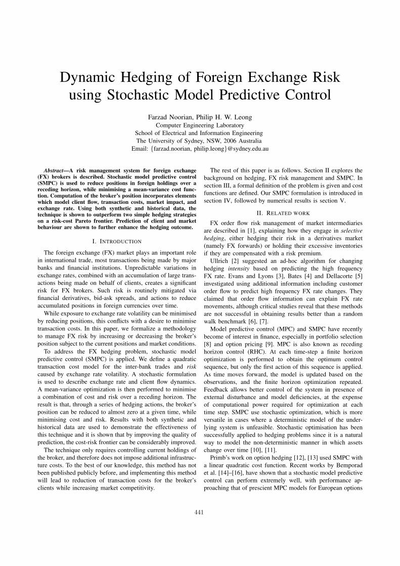
being updated at each time step based on observed marketconditions. The Monte-Carlo simulator generates scenariosbased on the models, which are then given to the stochasticoptimizer to obtain the optimal hedging action H. The firstvalue of H is hedged, which adds to the transaction cost.At the next time-step, FX rate changes cause changes in thevalue of broker’s open positions, generating profit or loss. Theprocess continues until the end-of-trading time is reached.

Fig. 1 illustrates the relationship of the proposed risk man-agement system to the rest of model. The hedging algorithmis summarised in algorithm 1.

Algorithm 1 SMPC Hedging Algorithmi 1while i N do

Update client flow model from historic dataUpdate FX rate model from market conditionsGenerate ⌘ scenarios for F and R for time t 2 [i, ..., N ]Compute the optimal H(i : n)Hedge by H(i)i i + 1

end while

V. RESULTS

In this section, two numerical examples are provided tocompare the SMPC hedging with two benchmark strategies,both of which consider the exchange rate and client flow asbeing unpredictable and therefore do not use this information.

The first benchmark strategy sets a hard limit xmax for thebroker’s position:

h(t) =

8

>

<

>

:

xmax � (x(t) + f(t)) x(t) + f(t) > xmax

x(t) + f(t)� xmax x(t) + f(t) < �xmax

0 otherwise(26)

By changing this limit, the strategy tries to move fromminimum risk (xmax = 0) to minimum cost (xmax = 1);however, as the limit passes a certain threshold, the transaction

●

●

●

●●●

●●●●

●●

●●

●●●

●

●

●

●

●

●

●

●●●●●

●●

●02

46

810

12

14

Hour of day

Clie

nt flo

w S

tandard

Devi

atio

n

7:00 11:00 15:00 19:00 23:00

Fig. 2. The synthetic client flow standard deviation vs. time.

cost caused by large end-of-trading session clearance imposesan additional cost to the broker.

The second strategy divides hedging instalments over allremaining trading hours to avoid market impact effects andadditional transaction costs; this is further parametrized by �as a risk aversion parameter:

h(t) = �(x(t) + f(t))(N � t)� + 1

N � t + 1(27)

where � = 1 gives the minimum risk and � = 0 results in theminimum cost.

It must be noted that the minimum cost is only for variationsof � 2 [0, 1] and not the global minima for transaction cost.Given full knowledge of client flow, one can use the followingequation to obtain the minimum theoretical transaction cost:

Cmin =NX

i=1

(�f)2 (28)

where f = 1

N

PNi=1

f(i). Minimum risk, in any case, is 0when h(t) = �f(t).

The experiments were implemented in the R programminglanguage [18] and used quadprog package [19] for quadraticprogramming.

A. Synthetic test and results

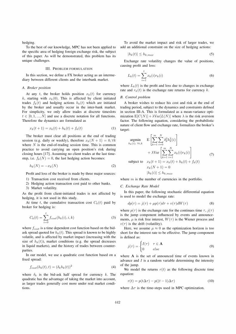
It has been observed that the clients exhibit a certainseasonality, e.g. more trades happen mid-day rather than atthe end-of-day hours. Therefore the client flow is modelled asa zero-mean heteroskedastic process, with a time-dependentvariance �2:

f(t) ⇠ N (0, �2(t)) (29)

We assume that f(i) and f(j) are independent for 8i 6= j.The client flow standard deviation, �(t), for synthetic data isshown in Fig. 2.

444

●●

●

●

●

●

●

●

●

●

●

●

●

●

●

●

●

●

●

●

●

●

●●

●

● ●●

●

●● ●

−3e+

07

−1e+

07

1e+

07

3e+

07

Hour of day

Em

ula

ted c

lient flo

w

7:00 11:00 15:00 19:00 23:00

●

●

●

●● ●

●

●

●

●

●

●

●

●

●●

●

●

●

●

●

●

● ●● ● ●

●● ●

●●

●

● ●

●

●

●

●

●

●

●

●

●

●

●

●

●

●

●

●

●

● ●●

●

●●

● ●●

●

● ●● ●

●

●

●

●

●

● ●

●

●

●

●

●

●

●

●

●

●

●

●

●

●

●

●●

●●

●

● ● ●●

●

●

●

●

●

●

●

●

●

●

●

●

●

● ●

●

●

● ●

●

●

●

●

●

●●

●

● ● ● ●●

●

●

●

●

●

●

●

●

●

●

●

●

●

●

●

●●

●

●

●

●

● ●●

●

●●

● ● ● ●

●

●

●

●

●

●

●

●

●

●

●●

●

●

●

●

●

●

●

●

●

●●

● ●

●

● ●●

● ● ●

●

●

●

●

●

●

●

●

●

●

●

●

●

●

●

●

●

●

●

●

●

●●

●

●●

●●

●

● ●●

●

●

●

●

●●

●

●

●

●

●

●

●

●

●

●

●

●

●

●

●

●

●

● ●

● ● ●●

●● ●

●

●

●

●

●

●

●

●

● ●

●

●

●

●

●

●

●

●

●

● ● ●

●

●

●●

●●

● ●

●●

●● ● ●

●●

●● ● ●

● ●

●

●●

●

●● ● ● ●

●●

●●

●● ●

● ● ●●

0.9

85

0.9

90

0.9

95

1.0

00

1.0

05

1.0

10

Hour of day

Em

ula

ted F

X r

ate

7:00 11:00 15:00 19:00 23:00

● ● ● ●●

● ●● ●

● ●● ● ●

● ●

● ● ●●

● ● ● ● ● ● ● ● ●

●

● ●

● ● ●● ● ●

●●

● ●● ●

● ●●

●

● ● ●● ● ●

●●

●●

●●

●●

● ●

●● ●

●● ●

●●

●● ●

●●

●● ●

●

●●

● ●● ●

●●

●●

● ●● ●

●

● ●●

● ●● ● ●

●●

●●

●●

●●

●● ●

●●

● ● ● ●● ●

● ●●

●●

●● ●

●● ● ● ●

●● ● ● ●

● ●●

●

●●

●●

●●

●

●●

● ●●

● ●●

● ●● ● ●

● ●● ●

●● ●

● ● ● ●

● ● ● ● ●●

● ● ● ● ●●

● ●

●●

●● ●

●● ● ● ● ●

●

●●

● ●

●●

● ●●

●●

●

●● ●

●● ●

●● ●

●

● ●●

● ● ●

●●

● ● ● ●● ● ● ●

●

●●

●●

●●

● ● ● ●● ●

● ● ●

● ●●

●●

● ● ● ●●

● ●● ●

● ●

●●

● ● ●● ●

●●

●

● ● ● ● ●

●

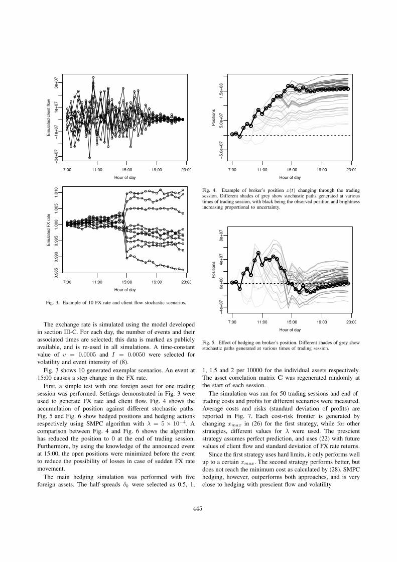
Fig. 3. Example of 10 FX rate and client flow stochastic scenarios.

The exchange rate is simulated using the model developedin section III-C. For each day, the number of events and theirassociated times are selected; this data is marked as publiclyavailable, and is re-used in all simulations. A time-constantvalue of v = 0.0005 and I = 0.0050 were selected forvolatility and event intensity of (8).

Fig. 3 shows 10 generated exemplar scenarios. An event at15:00 causes a step change in the FX rate.

First, a simple test with one foreign asset for one tradingsession was performed. Settings demonstrated in Fig. 3 wereused to generate FX rate and client flow. Fig. 4 shows theaccumulation of position against different stochastic paths.Fig. 5 and Fig. 6 show hedged positions and hedging actionsrespectively using SMPC algorithm with � = 5 ⇥ 10�4. Acomparison between Fig. 4 and Fig. 6 shows the algorithmhas reduced the position to 0 at the end of trading session.Furthermore, by using the knowledge of the announced eventat 15:00, the open positions were minimized before the eventto reduce the possibility of losses in case of sudden FX ratemovement.

The main hedging simulation was performed with fiveforeign assets. The half-spreads �k were selected as 0.5, 1,

●●●

●●

●

●

●●

●●

●●●

●

●●●●

●●●●●●●●●●●●●

−5.0

e+

07

5.0

e+

07

1.5

e+

08

Hour of day

Posi

tions

7:00 11:00 15:00 19:00 23:00

●●●

●●

●

●

●●

●●

●●●

●

●●●●

●●●●●●●●●●●●●

Fig. 4. Example of broker’s position x(t) changing through the tradingsession. Different shades of grey show stochastic paths generated at varioustimes of trading session, with black being the observed position and brightnessincreasing proportional to uncertainty.

●●

●

●

●

●

●

●

●

●●●

●

●●

●●

●●

●

●●●●●●●●●●●●

−4e+

07

0e+

00

4e+

07

8e+

07

Hour of day

Posi

tions

7:00 11:00 15:00 19:00 23:00

●●

●

●

●

●

●

●

●

●●●

●

●●

●●

●●

●

●●●●●●●●●●●●

Fig. 5. Effect of hedging on broker’s position. Different shades of grey showstochastic paths generated at various times of trading session.

1, 1.5 and 2 per 10000 for the individual assets respectively.The asset correlation matrix C was regenerated randomly atthe start of each session.

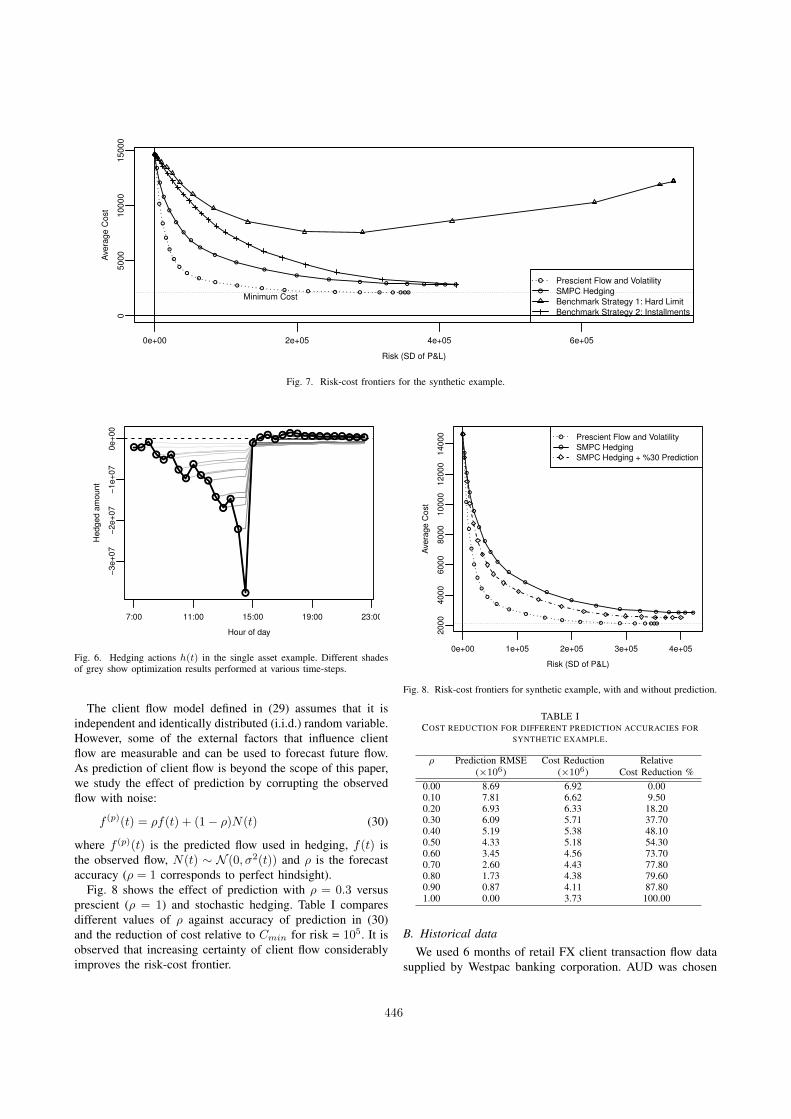
The simulation was ran for 50 trading sessions and end-of-trading costs and profits for different scenarios were measured.Average costs and risks (standard deviation of profits) arereported in Fig. 7. Each cost-risk frontier is generated bychanging xmax in (26) for the first strategy, while for otherstrategies, different values for � were used. The prescientstrategy assumes perfect prediction, and uses (22) with futurevalues of client flow and standard deviation of FX rate returns.

Since the first strategy uses hard limits, it only performs wellup to a certain xmax. The second strategy performs better, butdoes not reach the minimum cost as calculated by (28). SMPChedging, however, outperforms both approaches, and is veryclose to hedging with prescient flow and volatility.

445

●

0e+00 2e+05 4e+05 6e+05

05

00

01

00

00

15

00

0

Risk (SD of P&L)

Ave

rag

e C

ost

●●●●●●●●●●

●●

●

●

●

●

●

●

●

●

●

●●●●●●●●

●

●

●

●

●

●

●

●

●

●

●

●

●

Minimum Cost

●

●

Prescient Flow and VolatilitySMPC HedgingBenchmark Strategy 1: Hard LimitBenchmark Strategy 2: Installments

Fig. 7. Risk-cost frontiers for the synthetic example.

●●●

●●

●

●●

●

●●

●

●

●

●

●

●●●

●●●●●●●●●●●●●

−3e+

07

−2e+

07

−1e+

07

0e+

00

Hour of day

Hedged a

mount

7:00 11:00 15:00 19:00 23:00

●●●

●●

●

●●

●

●●

●

●

●

●

●

●●●

●●●●●●●●●●●●●

Fig. 6. Hedging actions h(t) in the single asset example. Different shadesof grey show optimization results performed at various time-steps.

The client flow model defined in (29) assumes that it isindependent and identically distributed (i.i.d.) random variable.However, some of the external factors that influence clientflow are measurable and can be used to forecast future flow.As prediction of client flow is beyond the scope of this paper,we study the effect of prediction by corrupting the observedflow with noise:

f (p)(t) = ⇢f(t) + (1� ⇢)N(t) (30)

where f (p)(t) is the predicted flow used in hedging, f(t) isthe observed flow, N(t) ⇠ N (0, �2(t)) and ⇢ is the forecastaccuracy (⇢ = 1 corresponds to perfect hindsight).

Fig. 8 shows the effect of prediction with ⇢ = 0.3 versusprescient (⇢ = 1) and stochastic hedging. Table I comparesdifferent values of ⇢ against accuracy of prediction in (30)and the reduction of cost relative to Cmin for risk = 105. It isobserved that increasing certainty of client flow considerablyimproves the risk-cost frontier.

●●●●●●●●●●

●

●

●

●

●

●

●

●

●

●

●

0e+00 1e+05 2e+05 3e+05 4e+05

2000

4000

6000

8000

10000

12000

14000

Risk (SD of P&L)

Ave

rage C

ost

●●●●●●●●●●

●

●

●

●

●

●

●

●

●

●

●

●●●●●●●

●

●

●

●

●

●

●

●

●

●

●

●

●

●●

●

Prescient Flow and VolatilitySMPC HedgingSMPC Hedging + %30 Prediction

Fig. 8. Risk-cost frontiers for synthetic example, with and without prediction.

TABLE ICOST REDUCTION FOR DIFFERENT PREDICTION ACCURACIES FOR

SYNTHETIC EXAMPLE.

⇢ Prediction RMSE Cost Reduction Relative(⇥10

6) (⇥10

6) Cost Reduction %0.00 8.69 6.92 0.000.10 7.81 6.62 9.500.20 6.93 6.33 18.200.30 6.09 5.71 37.700.40 5.19 5.38 48.100.50 4.33 5.18 54.300.60 3.45 4.56 73.700.70 2.60 4.43 77.800.80 1.73 4.38 79.600.90 0.87 4.11 87.801.00 0.00 3.73 100.00

B. Historical dataWe used 6 months of retail FX client transaction flow data

supplied by Westpac banking corporation. AUD was chosen

446

as the home currency and USD, EUR, NZD and JPY wereselected as foreign assets.

The client flow was filtered and aggregated to create 32half-hourly values per day. The first 2 month of data was usedto obtain model parameters of (29), and the next 4 monthswere used for outsample testing.

The exchange rate simulation was performed by fittinghistorical FX rates to the model of section III-C. Individualvariances v and correlation matrix C were computed from co-variances of the previous day, and jump component timingswere extracted from the publically available DailyFX eventcalendar [20]. Jump intensity was set to I = 10v. Only eventsclassified as high impact were considered in this simulationand the rest were discarded. The half-spread � for eachcurrency was selected as 0.5, 1, 2 and 1 per 10000 for USD,EUR, NZD and JPY respectively.

Two hundred (⌘ = 200) scenarios were generated perday for SMPC simulation. Cost and profit and loss werecomputed according to (3) and (6) respectively and werenormalized by the daily total value of transactions

P |f(i)|.The average normalized cost is reported on the vertical axisand the standard deviation of profit and loss is reported onhorizontal axis as risk. Run-time of the algorithm for eachtime-step was less than a second on a 3.4 GHz Intel Core-i7 machine, making it suitable for deployment in real-timesystems.

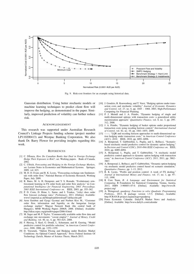
The average risk-cost curves for a simulation over 50 daysare shown in Fig. 9. Although SMPC hedging outperformsboth benchmark hedging algorithms, there is a significant gapbetween SMPC results and the prescient curve. This problemcan be traced to client modelling, where the simple model of(29) is not able to capture certain features such as the fat-taileddistribution of flow, and dependencies between adjacent timeperiods.

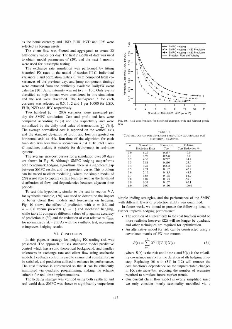
To test this hypothesis, similar to the test in section V-Afor synthetic example, (30) was used to determine the impactof better client flow models and forecasting on hedging.Fig. 10 shows the effect of prediction with ⇢ = 0.3 and⇢ = 0.6 versus prescient (⇢ = 1) and stochastic hedging,while table II compares different values of ⇢ against accuracyof prediction in (30) and the reduction of cost relative to Cmin

for normalized risk = 2.5. As with the synthetic test, increasing⇢ improves hedging results.

VI. CONCLUSION

In this paper, a strategy for hedging FX trading risk waspresented. The approach utilises stochastic model predictivecontrol which has a solid theoretical background, and handlesunknowns in exchange rate and client flow using stochasticmodels. Feedback control is used to ensure that constraints canbe satisfied, and prediction utilised to enhance its performance.The cost function is constructed so that it can be efficientlyminimised via quadratic programming, making the schemesuitable for real-time implementations.

The hedging strategy was verified using both synthetic andreal-world data. SMPC was shown to significantly outperform

0 2 4 6 8 10 12 14

0.1

00.1

50.2

00.2

50.3

00.3

50.4

0

Normalized Risk (0.0001 AUD per AUD)

Norm

aliz

ed C

ost

(0.0

001 A

UD

per

AU

D)

●●●●●

●

●

●

●

●

●

●

●

●

●

●

●●●●●

●●●●●●●●●

●

●

●

●

●

●

●

●

●

●

●

●●

●

SMPC HedgingSMPC Hedging + %30 PredictionSMPC Hedging + %60 PredictionPrescient Flow and Volatility

Fig. 10. Risk-cost frontiers for historical example, with and without predic-tion.

TABLE IICOST REDUCTION FOR DIFFERENT PREDICTION ACCURACIES FOR

HISTORICAL EXAMPLE.

⇢ Normalized Normalized RelativePrediction Error Cost Cost Reduction %

0.0 5.29 0.237 0.00.1 4.92 0.228 8.00.2 4.36 0.222 14.20.3 3.81 0.210 25.00.4 3.27 0.202 32.40.5 2.71 0.192 42.20.6 2.16 0.185 48.30.7 1.63 0.178 54.90.8 1.09 0.173 59.90.9 0.54 0.167 65.11.0 0.00 0.130 100.0

simple trading strategies, and the performance of the SMPCwith different levels of prediction ability was quantified.

In future work, we intend to pursue the following ideas tofurther improve hedging performance:

• The addition of a linear term to the cost function would bemore realistic; however (22) will no longer be quadraticand other techniques are required for optimization.

• An alternative model for risk can be constructed using acovariance matrix of FX rate returns:

R(t) =tX

i=1

XT (i)V (i)X(i) (31)

where R(t) is the risk until time t and V (i) is the volatil-ity covariance matrix for the duration of ith hedging time-step. Replacing (6) with (31) in (12) will remove thecost function’s dependence on the unpredictable changesin FX rate direction, reducing the number of scenariosrequired to simulate future market trends.

• Our current client flow model is overly simplified sincewe only consider hourly seasonality modelled via a

447

0 5 10 15 20 25

0.0

0.1

0.2

0.3

0.4

Normalized Risk (0.0001 AUD per AUD)

No

rma

lize

d C

ost

(0

.00

01

AU

D p

er

AU

D)

●●●●●●●●●●

●

●

●

●

●

●

●

●

●

●

●

●●●●●●

●

●

●

●

●

●

●

●

●

●

●●●●●

Minimum Cost●

●

Prescient Flow and VolatilitySMPC HedgingBenchmark Strategy 1: Hard LimitBenchmark Strategy 2: Installments

Fig. 9. Risk-cost frontiers for an example using historical data.

Gaussian distribution. Using better stochastic models ormachine learning techniques to predict client flow willimprove the hedging, as demonstrated in the paper. Simi-larly, improved prediction of volatility can further reducerisk.

ACKNOWLEDGEMENT

This research was supported under Australian ResearchCouncil’s Linkage Projects funding scheme (project numberLP110200413) and Westpac Banking Corporation. We alsothank Dr. Barry Flower for providing insights regarding thiswork.

REFERENCES

[1] C. DSouza, How Do Canadian Banks that Deal in Foreign ExchangeHedge Their Exposure to Risk?, ser. Working papers. Bank of Canada,2002.

[2] C. Ullrich, Forecasting and Hedging in the Foreign Exchange Markets,ser. Lecture Notes in Economics and Mathematical Systems. Springer,2009, vol. 623.

[3] M. D. D. Evans and R. K. Lyons, “Forecasting exchange rate fundamen-tals with order flow,” National Bureau of Economic Research, WorkingPaper, July 2009.

[4] R. Bates, M. A. H. Dempster, and Y. S. Romahi, “Evolutionary rein-forcement learning in FX order book and order flow analysis,” in Com-putational Intelligence for Financial Engineering, 2003. Proceedings.2003 IEEE International Conference on. IEEE, 2003, pp. 355–362.

[5] P. D. Corte, D. Rime, L. Sarno, and I. Tsiakas, “(why) does orderflow forecast exchange rates,” Preliminary, 2011. [Online]. Available:www3.imperial.ac.uk/fileupload/download/7.dellacorte.pdf

[6] Aron Gereben and Gyrgy Gyomai and Norbert Kiss M., “Customerorder flow, information and liquidity on the hungarian foreignexchange market,” Magyar Nemzeti Bank (the central bank ofHungary), MNB Working Papers 2006/8, 2006. [Online]. Available:http://ideas.repec.org/p/mnb/wpaper/2006-8.html

[7] M. Sager and M. P. Taylor, “Commercially available order flow data andexchange rate movements: ”caveat emptor”,” Journal of Money, Creditand Banking, vol. 40, no. 4, pp. 583–625, 2008.

[8] F. Herzog, S. Keel, G. Dondi, L. Schumann, and H. Geering, “Modelpredictive control for portfolio selection,” in American Control Confer-ence, 2006, 2006, pp. 1252–1259.

[9] D. Voesenek, “Option Pricing and Hedging under Realistic MarketConditions An Optimal Control Approach,” Swiss Federal Institute OfTechnology Zurich, Master of Science Thesis, March 2013.

[10] J. Gondzio, R. Kouwenberg, and T. Vorst, “Hedging options under trans-action costs and stochastic volatility,” Journal of Economic Dynamicsand Control, vol. 27, no. 6, pp. 1045 – 1068, 2003, High-PerformanceComputing for Financial Planning.

[11] P. J. Meindl and J. A. Primbs, “Dynamic hedging of single andmulti-dimensional options with transaction costs: a generalized utilitymaximization approach,” Quantitative Finance, vol. 8, no. 3, pp. 299–312, 2008.

[12] J. A. Primbs, “Dynamic hedging of basket options under proportionaltransaction costs using receding horizon control,” International Journalof Control, vol. 82, no. 10, pp. 1841–1855, 2009.

[13] ——, “LQR and receding horizon approaches to multi-dimensional op-tion hedging under transaction costs,” in American Control Conference(ACC), 2010. IEEE, 2010, pp. 6891–6896.

[14] A. Bemporad, T. Gabbriellini, L. Puglia, and L. Bellucci, “Scenario-based stochastic model predictive control for dynamic option hedging,”in Decision and Control (CDC), 2010 49th IEEE Conference on. IEEE,2010, pp. 6089–6094.

[15] A. Bemporad, L. Puglia, and T. Gabbriellini, “A stochastic modelpredictive control approach to dynamic option hedging with transactioncosts,” in American Control Conference (ACC), 2011, 2011, pp. 3862–3867.

[16] A. Bemporad, L. Bellucci, and T. Gabbriellini, “Dynamic option hedgingvia stochastic model predictive control based on scenario simulation,”Quantitative Finance, pp. 1–13, 2012.

[17] R. K. Lyons, “Profits and position control: A week of FX dealing,”Journal of International Money and Finance, vol. 17, no. 1, pp. 97–115, 1998.

[18] R Core Team, R: A Language and Environment for StatisticalComputing, R Foundation for Statistical Computing, Vienna, Austria,2013, ISBN 3-900051-07-0. [Online]. Available: http://www.R-project.org/

[19] A. Weingessel, quadprog: Functions to solve Quadratic ProgrammingProblems., 2013, R package version 1.5-5. [Online]. Available:http://CRAN.R-project.org/package=quadprog

[20] Forex Economic Calendar. DailyFX Market News and Analysis.[Online]. Available: http://www.dailyfx.com/calendar

448