Dynamic Games - darp.lse.ac.ukdarp.lse.ac.uk/pdf/EC202/Lecture_7_8.pdf · Dynamic Games All games...

Dynamic GamesEC202 Lectures VII & VIII

Francesco Nava

London School of Economics

January 2011

Nava (LSE) EC202 — Lectures VII & VIII Jan 2011 1 / 30

Summary

Dynamic Games:

Definitions:

Extensive Form GameInformation Sets and BeliefsBehavioral StrategySubgame

Solution Concepts:

Nash EquilibriumSubgame Perfect EquilibriumPerfect Bayesian Equilibrium

Examples: Imperfect Competition


Dynamic Games

All games discussed in previous lectures were static. That is:

A set of players taking decisions simultaneously

or not being able to observe the choices made by others

Today we relax such assumption by modeling the timing of decisions

In common instances the rules of the game explicitly define:

the order in which players move

the information available to them when they take their decisions

A way of representing such dynamic games is in their Extensive Form

The following definitions are helpful to define such notion


Basic Graph Theory

A graph consists of a set of nodes and of a set of branches

Each branch connects a pair of nodes

A branch is identified by the two nodes it connects

A path is a set of branches:

xk , xk+1 |k = 1, ...,m

where m > 1 and every xk is a different node of the graph.

A tree is a graph in which any pair of nodes is connected by exactlyone path

A rooted tree is a tree in which a special nodes designated as the root

A terminal node is a node connected by only one branch


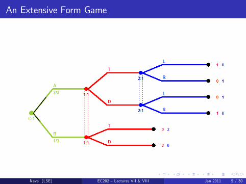
An Extensive Form Game


Extensive Form Games

An extensive form game is a rooted tree together with functions assigninglabels to nodes and branches such that:

1. Each non-terminal node has a player-label in C , 1, ..., n1, ..., n are the players in the gameNodes assigned to label C are chance nodesNodes assigned to label i 6= C are decision nodes controlled by i

2. Each alternative at a chance node has a label specifying itsprobability:

Chance probabilities are nonnegative and add to 1

3. Each node controlled by player i > 0 has a second label specifying i’sinformation state:

Thus nodes labeled i .s are controlled by i with information sTwo nodes belong to i .s iff i cannot distinguish them


Extensive Form Games

4. Each alternative at a decision node has move label:

If two nodes x , y belong to the same information set, for anyalternative at x there must be exactly one alternative at y with thesame move label

5. Each terminal node y has a label that specifies a vector of n numbersui (y)i∈1,...,n such that:

The number ui (y) specifies the payoff to i if the game ends at node y

6. All players have perfect recall of the moves they chose


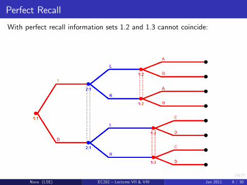
Perfect Recall

With perfect recall information sets 1.2 and 1.3 cannot coincide:


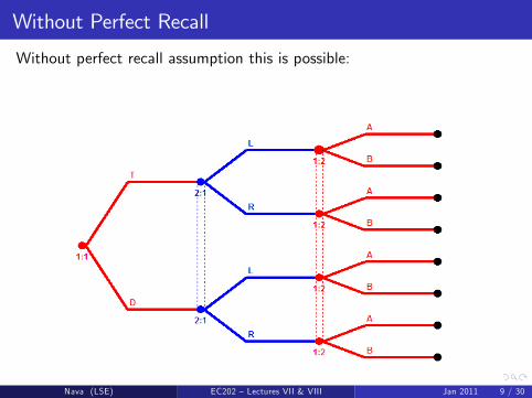
Without Perfect Recall

Without perfect recall assumption this is possible:


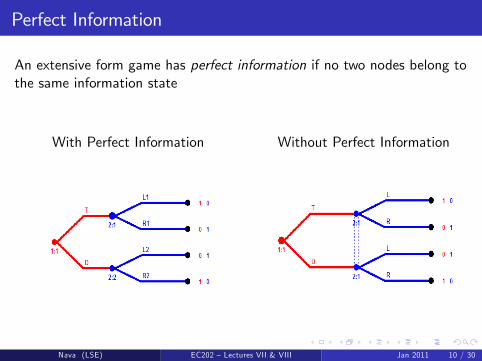
Perfect Information

An extensive form game has perfect information if no two nodes belong tothe same information state

With Perfect Information Without Perfect Information


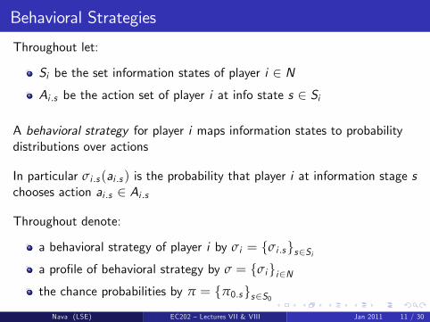
Behavioral Strategies

Throughout let:

Si be the set information states of player i ∈ NAi .s be the action set of player i at info state s ∈ Si

A behavioral strategy for player i maps information states to probabilitydistributions over actions

In particular σi .s (ai .s ) is the probability that player i at information stage schooses action ai .s ∈ Ai .s

Throughout denote:

a behavioral strategy of player i by σi = σi .ss∈Sia profile of behavioral strategy by σ = σii∈Nthe chance probabilities by π = π0.ss∈S0


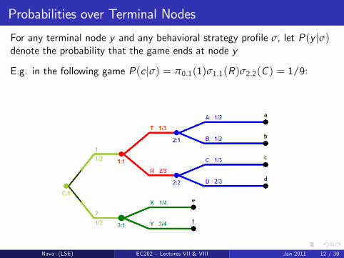
Probabilities over Terminal Nodes

For any terminal node y and any behavioral strategy profile σ, let P(y |σ)denote the probability that the game ends at node y

E.g. in the following game P(c |σ) = π0.1(1)σ1.1(R)σ2.2(C ) = 1/9:


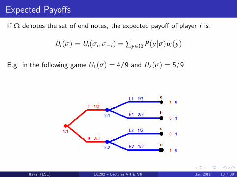
Expected Payoffs

If Ω denotes the set of end notes, the expected payoff of player i is:

Ui (σ) = Ui (σi , σ−i ) = ∑y∈Ω P(y |σ)ui (y)

E.g. in the following game U1(σ) = 4/9 and U2(σ) = 5/9


Nash Equilibrium

Definition (Nash Equilibrium —NE)A Nash Equilibrium of an extensive form game is any profile of behavioralstrategies such that:

Ui (σ) ≥ Ui (σ′i , σ−i ) for any σ′i ∈ ×s∈Si ∆(Ai .s )

Recall that σ′i is any mapping from information sets to probabilitydistributions over available actions

The definition of NE is as in strategic form games

What differs is the strategy (behavioral) that is expressed at every singledecision stage and not on profiles of decisions for every individual


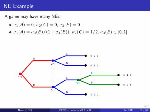
NE Example

A game may have many NEs:

σ1(A) = 0, σ2(C ) = 0, σ3(E ) = 0

σ1(A) = σ3(E )/(1+ σ3(E )), σ2(C ) = 1/2, σ3(E ) ∈ [0, 1]


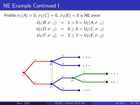
NE Example Continued I

Profile σ1(A) = 0, σ2(C ) = 0, σ3(E ) = 0 is NE since:

U1(B, σ−1) = 1 > 0 = U1(A, σ−1)

U2(D, σ−2) = 0 ≥ 0 = U2(C , σ−2)U3(F , σ−3) = 2 ≥ 2 = U3(E , σ−3)


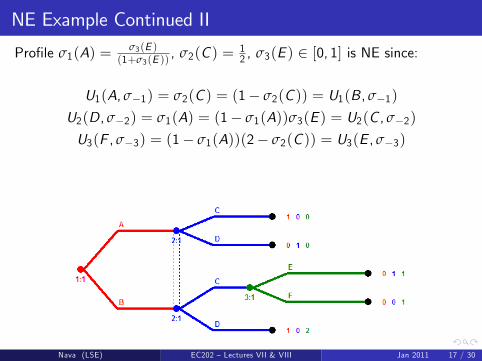
NE Example Continued II

Profile σ1(A) =σ3(E )

(1+σ3(E )), σ2(C ) = 1

2 , σ3(E ) ∈ [0, 1] is NE since:

U1(A, σ−1) = σ2(C ) = (1− σ2(C )) = U1(B, σ−1)

U2(D, σ−2) = σ1(A) = (1− σ1(A))σ3(E ) = U2(C , σ−2)

U3(F , σ−3) = (1− σ1(A))(2− σ2(C )) = U3(E , σ−3)


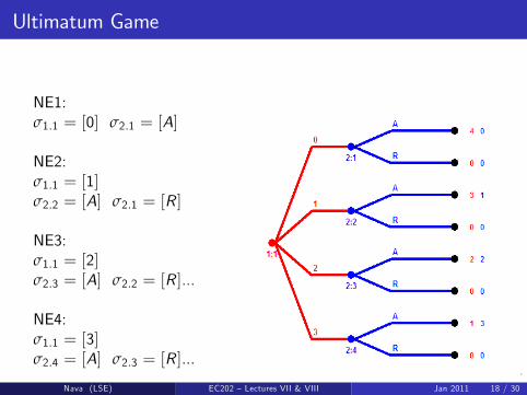
Ultimatum Game

NE1:σ1.1 = [0] σ2.1 = [A]

NE2:σ1.1 = [1]σ2.2 = [A] σ2.1 = [R ]

NE3:σ1.1 = [2]σ2.3 = [A] σ2.2 = [R ]...

NE4:σ1.1 = [3]σ2.4 = [A] σ2.3 = [R ]...


Ultimatum Game

Strategy σ1.1 = [0], σ2.1 = [A] is NE for any (σ2.2, σ2.3, σ2.4) since:

U1(0, σ2) = 4 > U1(a1, σ2) for any a1 ∈ 1, 2, 3U2(σ2, 0) = 0 = U2(a2, 0) for any a2 ∈ A,R4

Strategy σ1.1 = [0], σ2.2 = [A], σ2.1 = [R ] is NE for any (σ2.3, σ2.4) since:

U1(1, σ2) = 3 > U1(a1, σ2) for any a1 ∈ 0, 2, 3U2(σ2, 1) = 1 ≥ U2(a2, 1) for any a2 ∈ A,R4

A similar argument works for the other two proposed equilibria

Only the first two equilibria, however, involve threats that are credible,since player 2 would never want to refuse and offer worth at least 1$


Subgame Perfect Equilibrium

A successor of a node x is a node that can be reached from x for anappropriate profile of actions

Definition (Subgame)A subgame is a subset of an extensive form game such that:

1 It begins at a single node2 It contains all successors3 If a game contains an information set with multiple nodes then eitherall of these nodes belong to the subset or none does

Definition (Subgame Perfect Equilibrium —SPE)A subgame perfect equilibrium is any NE such that for every subgame therestriction of strategies to this subgame is also a NE of the subgame.


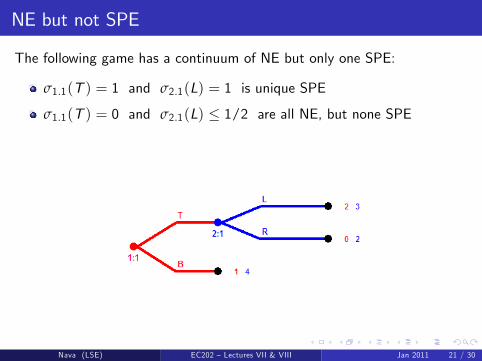
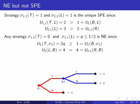
NE but not SPE

The following game has a continuum of NE but only one SPE:

σ1.1(T ) = 1 and σ2.1(L) = 1 is unique SPE

σ1.1(T ) = 0 and σ2.1(L) ≤ 1/2 are all NE, but none SPE


NE but not SPE

Strategy σ1.1(T ) = 1 and σ2.1(L) = 1 is the unique SPE since:

U1.1(T , L) = 2 > 1 = U1(B, L)

U2.1(L) = 3 > 2 = U2.1(R)

Any strategy σ1.1(T ) = 0 and σ2.1(L) = q ≤ 1/2 is NE since:

U1(T , σ2) = 2q ≥ 1 = U1(B, σ2)

U2(L,B) = 4 = 4 = U2.1(R,B)


Computing SPE —Backward Induction

Definition of SPE is demanding because it imposes discipline on behavioreven in subgames that one expects not to be reached

SPE however is easy to compute in perfect information games

Backward-induction algorithm provides a simple way:

At every node leading only to terminal nodes players pick actions thatare optimal for them if that node is reached

At all preceding nodes players pick an actions that optimal for them ifthat node is reached knowing how all their successors behave

And so on until the root of the tree is reached

A pure strategy SPE exists in any perfect information game


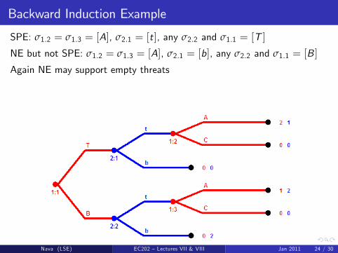
Backward Induction Example

SPE: σ1.2 = σ1.3 = [A], σ2.1 = [t], any σ2.2 and σ1.1 = [T ]

NE but not SPE: σ1.2 = σ1.3 = [A], σ2.1 = [b], any σ2.2 and σ1.1 = [B ]

Again NE may support empty threats


Duopoly: Stackelberg Competition

Implicit to both Cournot and Bertrand models was the assumption that noproducer could observe actions chosen by others before making a decision

In the Stackelberg duopoly model however:

Players choose how many goods to supply to the market (as Cournot)

One player moves first (the leader)

While the other player moves after having observed the decision ofthe leader (the follower)

Both players account for the distortions that their output choiceshave on equilibrium prices

To avoid empty threats restrict attention to the SPE of the dynamic game


Duopoly: Stackelberg Competition

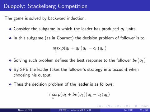
The game is solved by backward induction:

Consider the subgame in which the leader has produced qL units

In this subgame (as in Cournot) the decision problem of follower is to:

maxqFp(qL + qF )qF − cF (qF )

Solving such problem defines the best response to the follower bF (qL)

By SPE the leader takes the follower’s strategy into account whenchoosing his output

Thus the decision problem of the leader is as follows:

maxqLp(qL + bF (qL))qL − cL(qL)


Stackelberg Example

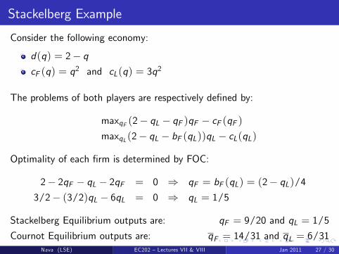
Consider the following economy:

d(q) = 2− qcF (q) = q2 and cL(q) = 3q2

The problems of both players are respectively defined by:

maxqF (2− qL − qF )qF − cF (qF )maxqL (2− qL − bF (qL))qL − cL(qL)

Optimality of each firm is determined by FOC:

2− 2qF − qL − 2qF = 0 ⇒ qF = bF (qL) = (2− qL)/43/2− (3/2)qL − 6qL = 0 ⇒ qL = 1/5

Stackelberg Equilibrium outputs are: qF = 9/20 and qL = 1/5Cournot Equilibrium outputs are: qF = 14/31 and qL = 6/31


Duopoly: Market Entry

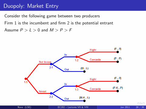
Consider the following game between two producers

Firm 1 is the incumbent and firm 2 is the potential entrant

Assume P > L > 0 and M > P > F


Duopoly: Market Entry

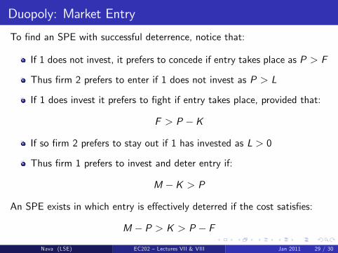
To find an SPE with successful deterrence, notice that:

If 1 does not invest, it prefers to concede if entry takes place as P > F

Thus firm 2 prefers to enter if 1 does not invest as P > L

If 1 does invest it prefers to fight if entry takes place, provided that:

F > P −K

If so firm 2 prefers to stay out if 1 has invested as L > 0

Thus firm 1 prefers to invest and deter entry if:

M −K > P

An SPE exists in which entry is effectively deterred if the cost satisfies:

M − P > K > P − F


Extra: Dynamics and Uncertainty

If an extensive form game does not display perfect information, subgameperfection cannot be imposed at every information set, but only onsubgames

In such games a further equilibrium refinement may help to highlight therelevant equilibria of the game by selecting those which Bayes rule

Definition (Perfect Bayesian Equilibrium —PBE)A perfect Bayesian equilibrium of an extensive form game consists of aprofile of behavioral strategies and of beliefs at each information set of thegame such that:

1 strategies form an SPE given the beliefs2 beliefs are updated using Bayes rule at each information set reachedwith positive probability


Dynamic Games - darp.lse.ac.ukdarp.lse.ac.uk/pdf/EC202/Lecture_7_8.pdf · Dynamic Games All games...

Documents

Transcript of Dynamic Games - darp.lse.ac.ukdarp.lse.ac.uk/pdf/EC202/Lecture_7_8.pdf · Dynamic Games All games...