DYNAMIC DECISION MODELS FOR MANAGING

THE MAJOR COMPLICATIONS OF DIABETES

by

Murat Kurt

B.S., Bogazici University, 2005

M.S. I.E., University of Pittsburgh, 2007

Submitted to the Graduate Faculty of

the Swanson School of Engineering in partial fulfillment

of the requirements for the degree of

Doctor of Philosophy

University of Pittsburgh

2012

UNIVERSITY OF PITTSBURGH

SWANSON SCHOOL OF ENGINEERING

This dissertation was presented

by

Murat Kurt

It was defended on

November 9, 2012

and approved by

Andrew J. Schaefer, PhD, Professor, Department of Industrial Engineering

M. Utku Unver, PhD, Professor, Department of Economics, Boston College

Mark S. Roberts, MD, MPP, Professor, Department of Health Policy and Management

Lisa M. Maillart, PhD, Associate Professor, Department of Industrial Engineering

Mustafa Akan, PhD, Assistant Professor, Tepper School of Business, Carnegie Mellon

University

Denis R. Saure, PhD, Assistant Professor, Department of Industrial Engineering

Dissertation Director: Andrew J. Schaefer, PhD, Professor, Department of Industrial

Engineering

ii

Copyright c© by Murat Kurt

2012

iii

DYNAMIC DECISION MODELS FOR MANAGING THE MAJOR

COMPLICATIONS OF DIABETES

Murat Kurt, PhD

University of Pittsburgh, 2012

Diabetes is the sixth-leading cause of death and a major cause of cardiovascular and renal

diseases in the U.S. In this dissertation, we consider the major complications of diabetes

and develop dynamic decision models for two important timing problems: Transplantation

in prearranged paired kidney exchanges (PKEs) and statin initiation.

Transplantation is the most viable renal replacement therapy for end-stage renal disease

(ESRD) patients, but there is a severe disparity between the demand and supply of kidneys

for transplantation. PKE, a cross-exchange of kidneys between incompatible patient-donor

pairs, overcomes many difficulties in matching patients with incompatible donors. In a typ-

ical PKE, transplantation surgeries take place simultaneously so that no donor may renege

after her intended recipient receives the kidney. We consider two autonomous patients with

probabilistically evolving health statuses in a PKE and model their transplant timing deci-

sions as a discrete-time non-zero-sum stochastic game. We explore necessary and sufficient

conditions for patients’ decisions to form a stationary-perfect equilibrium, and formulate a

mixed-integer linear programming (MIP) representation of equilibrium constraints to char-

acterize a socially optimal stationary-perfect equilibrium. We calibrate our model using

large scale clinical data. We quantify the social welfare loss due to patient autonomy and

demonstrate that the objective of maximizing the number of transplants may be undesirable.

Patients with Type 2 diabetes have higher risk of heart attack and stroke, and if not

treated these risks are confounded by lipid abnormalities. Statins can be used to treat such

abnormalities, but their use may lead to adverse outcomes. We consider the question of when

iv

to initiate statin therapy for patients with Type 2 diabetes. We formulate a Markov decision

process (MDP) to maximize the patient’s quality-adjusted life years (QALYs) prior to the

first heart attack or stroke. We derive sufficient conditions for the optimality of control-limit

policies with respect to patient’s lipid-ratio (LR) levels and age, and parameterize our model

using clinical data. We compute the optimal treatment policies and illustrate the importance

of individualized treatment factors by comparing their performance to those of the guidelines

in use in the U.S.

v

TABLE OF CONTENTS

1.0 INTRODUCTION . . . . . . . . . . . . . . . . . . . . . . . . . . . . . . . . . 1

1.1 Chronic and End-Stage Renal Diseases (ESRD) . . . . . . . . . . . . . . . . 2

1.2 Diabetes . . . . . . . . . . . . . . . . . . . . . . . . . . . . . . . . . . . . . . 6

1.3 Paired Kidney Exchanges . . . . . . . . . . . . . . . . . . . . . . . . . . . . 9

1.4 Relation Between Diabetes, ESRD and Cardiovascular Diseases . . . . . . . 10

1.5 Problem Statements and Contributions . . . . . . . . . . . . . . . . . . . . . 12

2.0 LITERATURE REVIEW . . . . . . . . . . . . . . . . . . . . . . . . . . . . . 15

2.1 Stochastic Games . . . . . . . . . . . . . . . . . . . . . . . . . . . . . . . . . 15

2.2 Game-Theoretic Applications in Healthcare . . . . . . . . . . . . . . . . . . 17

2.3 Kidney Exchanges and Organ Transplantation . . . . . . . . . . . . . . . . . 19

2.4 Operations Research Applications for Type 2 Diabetes . . . . . . . . . . . . 21

3.0 THE TIMING OF PREARRANGED PAIRED KIDNEY EXCHANGES

FOR SELF-INTERESTED PATIENTS . . . . . . . . . . . . . . . . . . . . 22

3.1 Model Formulation . . . . . . . . . . . . . . . . . . . . . . . . . . . . . . . . 23

3.2 Equilibrium Analyses . . . . . . . . . . . . . . . . . . . . . . . . . . . . . . 26

3.3 Numerical Experiments . . . . . . . . . . . . . . . . . . . . . . . . . . . . . 45

3.3.1 Data Sources and Parameter Estimation . . . . . . . . . . . . . . . . . 45

3.3.2 Welfare Loss Due to Patient Autonomy and Equilibrium Selection . . 50

3.3.3 Valuing Exchanges: An Example . . . . . . . . . . . . . . . . . . . . . 53

3.4 Conclusions . . . . . . . . . . . . . . . . . . . . . . . . . . . . . . . . . . . . 55

vi

4.0 THE OPTIMAL TIMING OF STATIN INITIATION FOR PATIENTS

WITH TYPE 2 DIABETES . . . . . . . . . . . . . . . . . . . . . . . . . . . 56

4.1 Model Formulation . . . . . . . . . . . . . . . . . . . . . . . . . . . . . . . . 57

4.2 Structural Properties . . . . . . . . . . . . . . . . . . . . . . . . . . . . . . . 62

4.3 Numerical Study . . . . . . . . . . . . . . . . . . . . . . . . . . . . . . . . . 76

4.3.1 Estimating Treatment-Effect and Transition Probabilities . . . . . . . 76

4.3.2 Estimating CHD and Stroke Probabilities . . . . . . . . . . . . . . . . 79

4.3.3 Numerical Results . . . . . . . . . . . . . . . . . . . . . . . . . . . . . 80

4.3.4 Sensitivity Analysis . . . . . . . . . . . . . . . . . . . . . . . . . . . . 82

4.3.5 Measuring the Violations of the Assumptions . . . . . . . . . . . . . . 84

4.3.6 Comparison with Current Treatment Guidelines . . . . . . . . . . . . 86

4.4 Conclusions . . . . . . . . . . . . . . . . . . . . . . . . . . . . . . . . . . . . 90

5.0 LIMITATIONS AND FUTURE RESEARCH . . . . . . . . . . . . . . . . 91

BIBLIOGRAPHY . . . . . . . . . . . . . . . . . . . . . . . . . . . . . . . . . . . . 95

vii

LIST OF TABLES

3.1 Boundaries of GFR ranges (in mL/min/1.73 m2) for numerical experiments. . 47

3.2 Patients’ maximum welfare losses from following a socially optimal equilibrium. 53

4.1 LR-range boundaries. . . . . . . . . . . . . . . . . . . . . . . . . . . . . . . . 78

4.2 Gender-specific LR-Range averages (LR`) . . . . . . . . . . . . . . . . . . . . 80

4.3 Patients’ maximum expected QALYs prior to their first terminal events. . . . 81

4.4 Patients’ QALY gains at the time of diagnosis when ω increases from 0.17 to

0.23. . . . . . . . . . . . . . . . . . . . . . . . . . . . . . . . . . . . . . . . . . 85

4.5 Patients’ QALY gains at the time of diagnosis when σ decreases from 0.05 to

0.01. . . . . . . . . . . . . . . . . . . . . . . . . . . . . . . . . . . . . . . . . . 85

4.6 Description of ATP III guidelines. . . . . . . . . . . . . . . . . . . . . . . . . 86

4.7 Patients’ expected QALY losses due to immediate initiation of treatment rather

than following the optimal policy of our model. . . . . . . . . . . . . . . . . . 88

4.8 Patients’ expected QALY losses due to following ATP III guidelines rather

than the optimal policy of our model. . . . . . . . . . . . . . . . . . . . . . . 89

4.9 Patients’ expected QALY losses due to following modified ATP III guidelines

rather than the optimal policy of our model. . . . . . . . . . . . . . . . . . . 89

viii

LIST OF FIGURES

1.1 Recent trend in demand and supply of kidneys for transplantation in the U.S.

[216]. . . . . . . . . . . . . . . . . . . . . . . . . . . . . . . . . . . . . . . . . 3

1.2 Graft and patient survival rates from kidney transplantation [216]. . . . . . . 4

1.3 Average median times on the waiting list with respect to blood-type [216]. . . 6

1.4 An illustration of a PKE. . . . . . . . . . . . . . . . . . . . . . . . . . . . . . 9

3.1 The data sources and references used in estimating daily-based health transi-

tion matrices. . . . . . . . . . . . . . . . . . . . . . . . . . . . . . . . . . . . 46

3.2 Social welfare loss and patients’ individual welfare losses due to patient autonomy. 51

3.3 Patient-donor characteristics for the matching example . . . . . . . . . . . . . 54

4.1 Division of the decision horizon into non-stationary and stationary subhorizons. 60

4.2 State transition diagram at epoch t ∈ T ′ under treatment status m ∈M. . . 61

4.3 Optimal LR-range thresholds (`∗t ) to initiate statin treatment for the base case. 82

4.4 Sensitivity of the male patient’s optimal policy with respect to σ for the base

case value of ω. . . . . . . . . . . . . . . . . . . . . . . . . . . . . . . . . . . . 83

4.5 Sensitivity of the female patient’s optimal policy with respect to σ for the base

case value of ω. . . . . . . . . . . . . . . . . . . . . . . . . . . . . . . . . . . . 83

4.6 Sensitivity of patients’ optimal policies with respect to ω for the base case

value of σ. . . . . . . . . . . . . . . . . . . . . . . . . . . . . . . . . . . . . . 84

ix

ACKNOWLEDGMENTS

in memory of Dr. Seth Bonder...

to my parents...

It has been a long journey. I would like to thank all my friends in Pittsburgh for making this

journey an enjoyable experience for me. I am grateful to the former and current wonderful

staff of the department, especially to Richard Brown, George Harvey, Minerva Pilachowski

and Jim Segneff, for providing immediate administrative and technical support throughout

my graduate studies.

Throughout my PhD study, I had the opportunity to collaborate with several great pro-

fessors from various disciplines. I am grateful to Professors Utku Unver, Brian Denton and

Jeffrey Kharoufeh for their guidance, unconditional motivational support, and excellent tech-

nical and editorial advice. I also thank Professors Mustafa Akan and Denis Saure for serving

on my dissertation committee, and Professors Lisa Maillart, Mark Roberts, Mainak Mazum-

dar, Matt Bailey, Brady Hunsaker and Oleg Prokopyev for enriching my knowledge during

my graduate studies and preparing me towards a successful dissertation. I am especially in-

debted to Professor Bopaya Bidanda for welcoming me into his office and patiently listening

to me on several occasions. His warm support was instrumental for me to circumvent my

times of confusion.

Last, but most, no words can describe how thankful I am to my advisor, Professor Andrew

Schaefer. I would like to express my sincere gratitude for his guidance, encouragement and

generous financial support. His remarkable enthusiasm on my research was a prominent

factor motivating me towards my goals. His flexibility, understanding and patience as a

mentor are beyond the limits of my appreciation and I feel very lucky to have his support

behind me.

x

1.0 INTRODUCTION

Healthcare is the largest single industry in the U.S. Elevated healthcare costs pose major

social and economic problems in the U.S. and force several cost-saving measures by state

and private agencies. Total national health expenditures accounted for 17.6% of the Gross

Domestic Product in 2010 and this share is expected to grow to 19.8% by 2020 [34]. National

health expenditure per person of the U.S., which exceeded $8,000 in 2009, is the highest

among all member states of the World Health Organization [233], and is expected to be

around $14,000 by 2020 with the aging population [34].

Increasing healthcare costs and economic challenges have received considerable attention

from academics and the media, and motivated a significant amount of research over the last

two decades. Operations Research (OR) techniques have found a variety of applications in

healthcare. These applications help develop new methodologies while improving the state

of the art in modeling and optimization techniques. They also inform practitioners on how

to make use of raw data to make better decisions and to address public policy concerns.

Examples of OR applications in healthcare include demand forecasting, hospital capacity

planning, patient and workforce scheduling, staffing emergency departments, locating emer-

gency service facilities, immunization and vaccine selection, organ allocation, and cancer

treatment planning, among several others. Earlier and more recent surveys summarize the

vast literature of OR applications in healthcare and highlight contemporary issues at the

intersection of OR and healthcare along with current challenges and emerging research ac-

tivities [24, 52, 68, 85, 110, 116, 127, 145, 147, 154, 162, 190].

1

1.1 CHRONIC AND END-STAGE RENAL DISEASES (ESRD)

In a healthy patient, kidneys perform key functions such as monitoring and regulating body

fluids, balancing electrolytes and filtering the blood. Chronic kidney disease (CKD) is the

progressive and irreversible loss of renal functionality over a period of months or years and

divided into five stages of severity [207].

ESRD, the last stage of CKD, typically occurs when the kidneys’ functionality is less

than 10 % of normal. It is the ninth-leading cause of death in the U.S. and has grown

alarmingly in the last decade [207]. Currently, more than 500,000 Americans have ESRD

and more than 26 million Americans are at increased risk of developing the disease [41]. The

size of the ESRD population is projected to grow to 2.24 million by 2030 and each year more

than 100,000 people experience a kidney failure in the U.S. [203, 210]. The total cost of

ESRD in the U.S. was around $30 billion in 2009 [209].

ESRD can result in death if not treated. There are three viable treatment alternatives

for ESRD patients: Hemodialysis, peritoneal dialysis and transplantation. Hemodialysis

is the most common renal replacement therapy and typically requires a patient to visit a

clinical center several times a week to have her blood cleaned. Although the procedure is

safe, several complications such as hypotension, cardiac arrhythmias and muscle cramps can

occur during the process of filtering blood [44].

In peritoneal dialysis, a filtering fluid is embedded into the patient’s body [150]. Peri-

toneal dialysis is cheaper than hemodialysis but yields almost equal survival rates as hemodial-

ysis. Especially for nondiabetic and young diabetic ESRD patients, it may have a lower risk

of death because of its superior preservation of residual kidney functionality. Despite such

advantages, the use of peritoneal dialysis is less common compared to hemodialysis [115, 128].

Due to insufficient supply of kidneys for transplantation, dialysis is a common interme-

diary step for ESRD patients. However, transplantation is the preferred choice of treatment

as it allows patients resume their regular activities with a higher quality of life than dialysis

by providing improved long-term survival rates [112, 228, 229].

2

In the U.S., an ESRD patient must join a waiting list administered by the United Network

for Organ Sharing (UNOS), a scientific and educational nonprofit organization, to be eligible

for a cadaveric kidney transplantation [215]. The current policy has been active for more

than two decades and prioritizes patients based on a scoring rule which takes several factors

into account, including the waiting time on the list and the quality of the match. Details

for the current cadaveric kidney allocation policy can be found in Organ Procurement and

Transplantation Network (OPTN) website [160]. As clear from Figure 1.1, the supply of

kidneys for transplantation is far below the waiting list additions. Currently, more than

90,000 patients in the U.S. are awaiting a kidney transplant, but in 2010, 4850 patients died

while waiting on the list and only 16,900 patients received transplants, 6,200 of which were

from living-donors [216].

0

5,000

10,000

15,000

20,000

25,000

30,000

35,000

40,000

1995 1998 2001 2004 2007 2010

Deaths while Waiting

Waiting List Additions

Cadaveric Transplants

Living-donor Transplants

Year

Figure 1.1: Recent trend in demand and supply of kidneys for transplantation in the U.S.

[216].

Because people can function normally on only one kidney, it is also possible for an

ESRD patient to receive an organ from a living-donor and transplants from such donors

generally yield better survival outcomes than those from cadaveric transplants (see Figure

3

65

70

75

80

85

90

95

100

Surv

ival

Rat

e (

%)

1-year

3-year

5-year

Graft Patient

Cadaveric Transplants Living-donor Transplants

Graft Patient

Figure 1.2: Graft and patient survival rates from kidney transplantation [216].

1.2). In fact there is a universal agreement in the transplant community that a living-donor

kidney transplant is the preferred course of treatment for ESRD patients [80, 205]. A kidney

transplanted from a living-donor is much preferred to a cadaveric kidney. In general, a

cadaveric kidney transplant may be subject to some degree of trauma and this trauma may

negatively affect the time between the moment the kidney stops functioning in the donor

and begins functioning in the transplant recipient. In some extreme cases, it may take a

few weeks for a cadaveric kidney transplant to function properly and the patient may need

dialysis until then. There are additional benefits of living-donor transplants, too. A living

kidney donation from a close relative, such as a sister or a brother, can yield an excellent

tissue-type match for the recipient thereby reducing the risk of kidney rejection. Also, a

living kidney donation gives the patient, donor, and possibly their families the flexibility to

plan the timing of surgery conveniently [208].

4

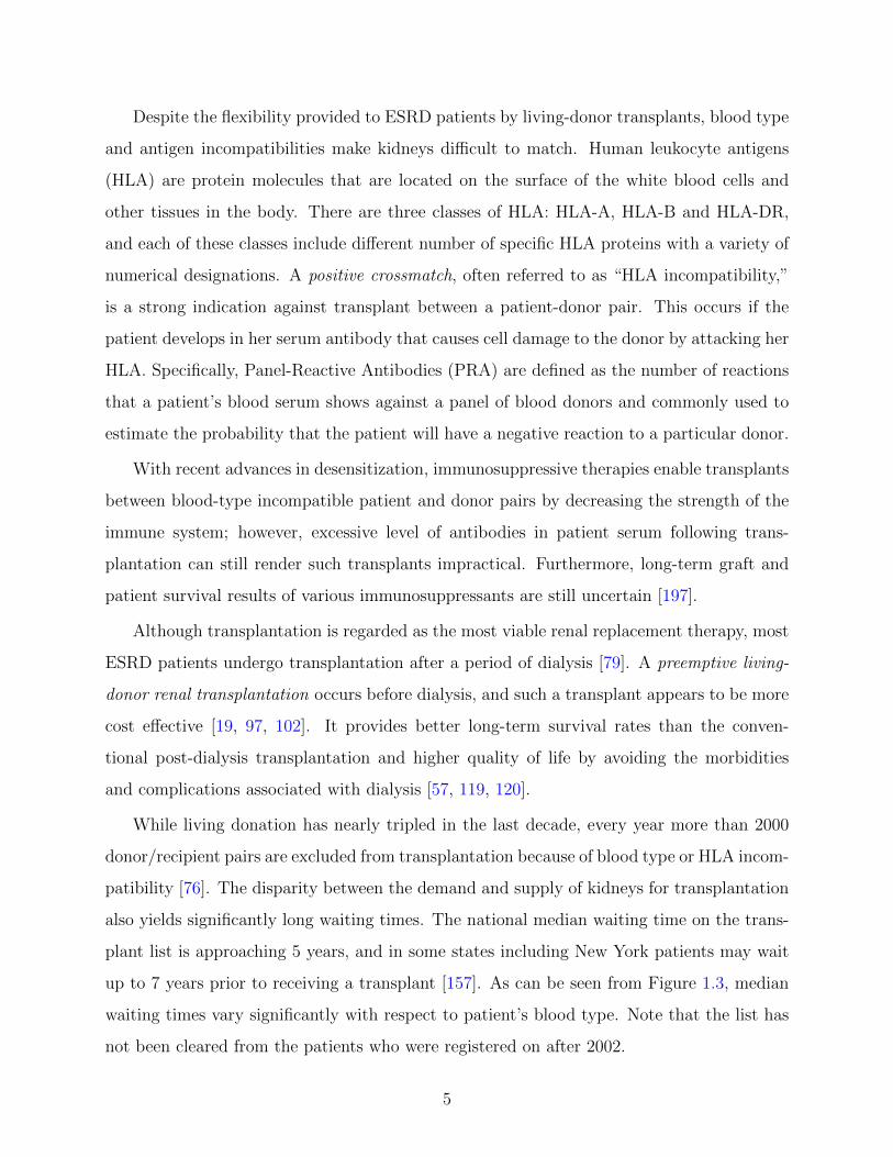
Despite the flexibility provided to ESRD patients by living-donor transplants, blood type

and antigen incompatibilities make kidneys difficult to match. Human leukocyte antigens

(HLA) are protein molecules that are located on the surface of the white blood cells and

other tissues in the body. There are three classes of HLA: HLA-A, HLA-B and HLA-DR,

and each of these classes include different number of specific HLA proteins with a variety of

numerical designations. A positive crossmatch, often referred to as “HLA incompatibility,”

is a strong indication against transplant between a patient-donor pair. This occurs if the

patient develops in her serum antibody that causes cell damage to the donor by attacking her

HLA. Specifically, Panel-Reactive Antibodies (PRA) are defined as the number of reactions

that a patient’s blood serum shows against a panel of blood donors and commonly used to

estimate the probability that the patient will have a negative reaction to a particular donor.

With recent advances in desensitization, immunosuppressive therapies enable transplants

between blood-type incompatible patient and donor pairs by decreasing the strength of the

immune system; however, excessive level of antibodies in patient serum following trans-

plantation can still render such transplants impractical. Furthermore, long-term graft and

patient survival results of various immunosuppressants are still uncertain [197].

Although transplantation is regarded as the most viable renal replacement therapy, most

ESRD patients undergo transplantation after a period of dialysis [79]. A preemptive living-

donor renal transplantation occurs before dialysis, and such a transplant appears to be more

cost effective [19, 97, 102]. It provides better long-term survival rates than the conven-

tional post-dialysis transplantation and higher quality of life by avoiding the morbidities

and complications associated with dialysis [57, 119, 120].

While living donation has nearly tripled in the last decade, every year more than 2000

donor/recipient pairs are excluded from transplantation because of blood type or HLA incom-

patibility [76]. The disparity between the demand and supply of kidneys for transplantation

also yields significantly long waiting times. The national median waiting time on the trans-

plant list is approaching 5 years, and in some states including New York patients may wait

up to 7 years prior to receiving a transplant [157]. As can be seen from Figure 1.3, median

waiting times vary significantly with respect to patient’s blood type. Note that the list has

not been cleared from the patients who were registered on after 2002.

5

0

500

1000

1500

2000

2500

Me

dia

n W

aiti

ng

Tim

e o

n t

he

Wai

tin

g Li

st (

in d

ays)

Blood Type

2000

2001

2002

O A B AB

Figure 1.3: Average median times on the waiting list with respect to blood-type [216].

Because the sale and acquisition of organs are illegal under the National Organ Transplant

Act of 1984 and the Uniform Anatomical Gift Act of 1987 [50], the difficulties in matching

patient-donor pairs motivated new clinical strategies to alleviate the shortage of kidneys and

to reduce the productivity losses due to long waiting times on dialysis [131, 144, 179, 232].

1.2 DIABETES

Diabetes mellitus, usually called diabetes, is the sixth-leading cause of death and a major

underlying cause of cardiovascular complications in the U.S. [134]. According to Ameri-

can Diabetes Association (ADA), there are currently more than 20 million Americans with

diabetes [15], and this number is expected to grow to 39 million by 2050 [91].

6

There are two types of diabetes: Type 1 and Type 2. Type 1 diabetes, also known as

insulin-dependent diabetes, occurs when pancreas produces very little or no insulin. On

the other hand, Type 2 diabetes, which is also called non insulin-dependent diabetes, occurs

with insulin resistance combined with relative insulin deficiency. In Type 2 diabetes although

pancreas produces insulin, body cannot use it properly. Because of this inefficiency, patients

often have difficulty in maintaining their blood glucose levels within healthy ranges. While

Type 1 diabetes usually occurs in children, Type 2 diabetes is more common among adults,

especially those over 40. In the U.S., approximately 90% of the diabetes cases are of Type

2 [16].

Type 2 diabetes has several significant complications, including coronary heart disease

(CHD), stroke, kidney failure, amputation, and blindness, all of which can result in disabil-

ities and work losses leading to poor productivity levels [143, 163]. These complications not

only affect the patients’ health-related quality of life but also account for a sizable portion

of the total healthcare costs to society [42, 206]. Of these complications, CHD and stroke

represent the leading causes of diabetic deaths in the U.S. [15]. Because Type 2 diabetes

can increase the patient’s CHD and stroke risks by a factor of five, they carry significant

importance for physicians in making treatment decisions [22, 106, 121, 196].

Lipid abnormalities increase the risk of CHD and stroke in patients with Type 2 diabetes

[108, 218]. The cholesterol profile of a patient is usually assessed by her triglycerides and three

types of cholesterol: Total cholesterol (TC), low-density lipoproteins (LDL) and high-density

lipoproteins (HDL). Among these, triglycerides are the main form of fat in bloodstream and

considered to be a positive risk factor for CHD. Elevated TC and LDL, which is the main

source of artery clogging plaque and referred to as “bad cholesterol,” increase the overall

risk of CHD and stroke. In contrast, HDL, which is also called “good cholesterol,” works

to extract cholesterol from the artery walls and dispose them through the liver. Therefore,

high levels of HDL are more desirable to reduce the risk of CHD. Elevated TC and depressed

HDL have been reported in clinical trials to increase the overall risk of CHD and stroke.

The ratio of TC to HDL, defined as the “lipid ratio” (LR), is a strong predictor of CHD and

stroke risks, but this ratio can vary significantly and unpredictably over time [75, 222, 226].

7

Several published risk models try to predict CHD and stroke probabilities for patients

with Type 2 diabetes based on their cholesterol levels and other risk factors. The most

widely used of these models was calibrated on data from the United Kingdom Prospective

Diabetes Study (UKPDS) [107, 198, 213]. The UKPDS model is based on a 20-year surveil-

lance of over 5,000 patients in the U.K and it predicts CHD and stroke probabilities over

time using several risk factors, including age, gender, ethnicity, smoking status, cholesterol,

systolic blood pressure (SBP) and glycated hemoglobin (HbA1c) levels. While other pre-

dictive models have been developed, e.g. the Framingham model [17] and the Archimedes

model [60, 61], the UKPDS model is unique in proposing risk equations specific to patients

with Type 2 diabetes.

Clinical trials have shown that cholesterol management using statins reduces CHD and

stroke risks [27, 37, 39, 40, 58]. A primary goal of managing Type 2 diabetes has been

the control of blood glucose levels, however more recently the importance of cardiovascular

risk has been emphasized [192, 214] and the complexity of treatment decisions has led to

the development of several national treatment guidelines with differing recommendations

[28, 67, 135, 136, 137, 141] (See Shah et al. [186] for a comparative effectiveness of these

guidelines). For instance, current U.S. guidelines, which is also known as Adult Treatment

Panel (ATP) III, and its variants [136] classify the patients with respect to their 10-year

CHD risks and set a specific treatment target for LDL levels in each of these categories.

Alternatively, the U.K. guidelines [28] recommend initiating lipid lowering agents such as

statins when the patient’s 10-year CHD risk exceeds 20%, and New Zealand guidelines

[141] make the same recommendation when the patient’s 5-year CHD risk exceeds 15%.

Conservatively, some recent U.S. guidelines [15, 192] recommend initiating statins in all

patients with Type 2 diabetes irrespective of their long-term CHD risks. Despite the effects

of cholesterol build-up in the arteries on a patient’s stroke risk, in addition to the differences

among the guidelines’ treatment policies, it is also notable that there is no guideline in

practice that takes the patient’s stroke risk into account for its treatment recommendations.

Although statin treatment reduces the risks of CHD and stroke, it can have serious side

effects, including muscle diseases, myopathy and liver problems. Other effects have also

been reported, such as headaches, nausea, fever, fatigue, shortness of breath, memory loss,

8

sexual dysfunction, skin problems, irritability, and effects on nervous and immunity systems

[151, 152, 153, 211]. Therefore, treatment guidelines should weigh the benefits of using

statins in reducing CHD and stroke risks against its side effects in making recommendations

and identifying the groups that would benefit most from the treatment.

1.3 PAIRED KIDNEY EXCHANGES

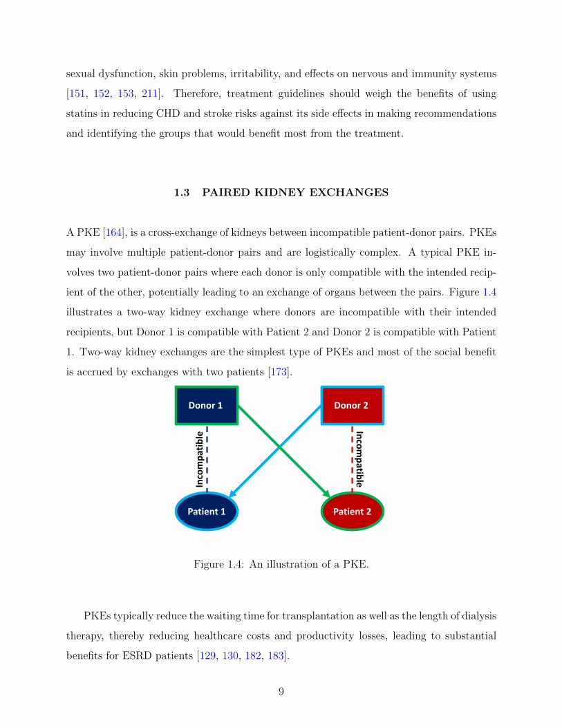
A PKE [164], is a cross-exchange of kidneys between incompatible patient-donor pairs. PKEs

may involve multiple patient-donor pairs and are logistically complex. A typical PKE in-

volves two patient-donor pairs where each donor is only compatible with the intended recip-

ient of the other, potentially leading to an exchange of organs between the pairs. Figure 1.4

illustrates a two-way kidney exchange where donors are incompatible with their intended

recipients, but Donor 1 is compatible with Patient 2 and Donor 2 is compatible with Patient

1. Two-way kidney exchanges are the simplest type of PKEs and most of the social benefit

is accrued by exchanges with two patients [173].

Patient 1 Patient 2

Inco

mp

atib

leIn

com

patib

le

Donor 1 Donor 2

Figure 1.4: An illustration of a PKE.

PKEs typically reduce the waiting time for transplantation as well as the length of dialysis

therapy, thereby reducing healthcare costs and productivity losses, leading to substantial

benefits for ESRD patients [129, 130, 182, 183].

9

PKEs have grown rapidly over the last two decades to overcome the difficulties in match-

ing kidneys [184] and it has been estimated that they can raise the number of transplants

by up to 90 % [173].

Since their conceptual proposal in late 80s, PKEs have attracted considerable focus from

media and the scientific community. The significant potential of PKEs [171, 184, 185] has

led to the establishment of several regional kidney exchange clearinghouses in the U.S.,

Korea [148, 149] and the Netherlands [49] to organize the registry of patients and donors

[13, 140]. These consortia expand the pool of living-donors and develop programs under

which incompatible patient-donor pairs are identified and cross-matched to other pairs and

altruistic donors [118]. Building such programs has compelled the development of advanced

algorithms to match patients with donors [100, 103] and it has been estimated that includ-

ing even compatible patient-donor pairs in the expansion pools can yield remarkably better

matching rates [77]. More recently, a national pilot kidney exchange program joining all

UNOS-approved kidney exchange clearinghouses has been launched to facilitate a more ef-

ficient network for exchanges between incompatible patient-donor pairs [158, 159]. Despite

all efforts PKEs have been grossly underutilized in the U.S. [43, 184, 231].

Another approach to the kidney shortage is an indirect kidney exchange or paired list

exchange [78, 133]. In such an exchange, a patient is given a higher priority on the cadaveric

kidney waiting list in exchange for her donor agreeing to donate a kidney to another patient

on the waiting list. There are ethical objections to indirect exchanges because of the potential

harm to patients without living-donors and those with O blood type, who are in fact the

hardest to match [4, 168, 169, 220, 238].

1.4 RELATION BETWEEN DIABETES, ESRD AND CARDIOVASCULAR

DISEASES

Because of the vascular abnormalities, diabetes is the leading cause of ESRD in the U.S.

and accounts for more than 44 % of new ESRD cases every year [33] and more than 50,000

diabetic patients in the U.S. are expected to experience ESRD eventually [32].

10

Kidneys contain thousands of nephrons which synthesize several proteins including al-

bumin. In the presence of diabetes, the small blood vessels in the kidneys are injured, and

high levels of blood sugar make the kidneys filter too much blood. With this extra filtering,

the nephrons thicken and become scarred, and the kidneys begin releasing small quantitites

of albumin into the urine. As the quantities of albumin become larger than normal, the

patient develops renal disease. Diabetes can also cause difficulty in emptying the bladder

and pressure resulting from a full bladder can injure the kidneys [138].

Tests can often detect signs of renal disease in the early stages and patients are recom-

mended to have a urine test at least once a year [14]. Because the urine test seeks small

quantitites of albumin in the urine, it is also called microalbuminuria test. If there is any

doubt, urine test can be followed by a kidney biopsy to confirm the diagnosis; however,

biopsy is not recommended as the first line of screening [86].

CKD and cardiovascular complications of diabetes are strongly related to each other in

that cardiovascular diseases (CVDs) can lead to CKD, and CKD can result in cardiovascular

complications. While CVDs are most effective in the early stages of CKD, majority of the

ESRD patients die because of a cardiovascular complication. Several abnormalities common

to ESRD also play a key role in patient’s development of a CVD, high blood pressure, high

blood cholesterol, excessive parathyroid hormone, to name a few [38]. Although there is no

way to cure renal disease and CVDs, they are often treatable during the early stages through

a systematic control of blood glucose and blood pressure. Usually, lowering blood pressure

with ACE inhibitors and angiotensin receptor blockers (ARBs) is the best way of protecting

kidneys from damage. Following a healthy low-fat diet and exercising regularly also help

slow down the progression of CKD and CVDs [72].

Even when diabetes is controlled, it can lead to kidney failure. People with diabetes used

to be excluded from dialysis and kidney transplantation, because the disease was increasing

the risk of bacterial and fungal infections in transplant recipients and the damage caused by

the disease was offsetting the benefits of dialysis and transplantation. Recently, with better

control of diabetes, doctors do not hesitate to offer dialysis and transplantation to diabetic

patients [104].

11

Diabetic patients who approach ESRD are not only subject to traditional cardiovascular

risk factors such as high blood pressure and high blood glucose, but also kidney disease-

related risk factors, such as anemia, uremia toxins, abnormal mineral metabolism, inflam-

mation and malnutrition [224]. Combination of such risk factors may further aggravate the

adverse cardiovascular risk profile. Therefore, although post-transplant graft survivals are

about the same in diabetic and nondiabetic patients, diabetic patients who are eligible to

receive a kidney transplant are recommended to transplant preemptively before initiating

dialysis [23, 56, 194].

1.5 PROBLEM STATEMENTS AND CONTRIBUTIONS

This dissertation concentrates on the timing of prearranged PKEs for autonomous and self-

interested patients with uncertain and dynamic health, and the timing of the initiation of

statin therapy for patients with Type 2 diabetes.

Current practice in PKE aims to maximize only the number of transplants and favors

immediate exchange. However, an early transplantation may fail to maximize the residual

renal functionality. Due to ethical barriers, in a typical PKE, transplantation surgeries take

place simultaneously so that no donor can withdraw her consent after her intended recipient

receives the kidney from the other donor. Therefore, the timing of the exchange requires some

form of an agreement between the pairs and determining proper edge weights that consider

the timing aspect of the exchange requires a decision model with two self-interested patients.

The optimization of the timing of a transplant for a single patient has been well studied in

the literature as reviewed in Chapter 2, however the models existing in the literature do not

apply to the timing of PKEs.

In Chapter 3, our contribution to the literature is two-fold. First, following current

clinical practice, we assume simultaneous transplantation surgeries and develop a competitive

decision model for the patients’ transplant timing decisions in prearranged PKEs. Second,

we analyze the resulting Nash equilibria in time-homogeneous strategies. While a complete

characterization of such equilibria is computationally prohibitive, we consider the issue of

12

equilibrium selection from a central-decision maker’s point of view and develop MIP models

for a systematic computation of the socially optimal equilibria and welfare loss borne by

patient autonomy.

Lipid abnormalities increase the risk of CHD and stroke in patients with Type 2 dia-

betes. Statins can be used to treat these abnormalities, but may have adverse side effects.

Cardiovascular risk models serve as a guide to clinicians for selecting the type of intervention

and the aggressiveness of treatment. However, their use in practice has focused on providing

raw information about the risk of complications and there has been little direction on how

to use this information to make treatment decisions that balance the trade-off between the

benefits of statins in cardiovascular risk reduction with the side effects of treatment.

In Chapter 4, our contribution to the literature is two-fold. First, we address the trade-off

between the benefits and side effects of statin treatment through a dynamic decision model.

More precisely, we develop an MDP model to optimize the start time of a statin therapy as

a function of time and the patient’s LR level. The treatment policies that we provide offer

individualized guidelines and may motivate the patients to adhere to prescribed treatment

regimens. The implications of our model may enhance the results of various clinical trials

and help physicians design more patient-focused cholesterol treatment guidelines through

explicit consideration of disutility of using statins. Second, we derive sufficient conditions

for the patient’s optimal policy to exhibit a threshold structure, and characterize how such

limits change with respect to patient’s age. These conditions have two important character-

istics. First, they provide analytical evidence to the structure of the treatment guidelines in

practice. Second, they relax some of the strong assumptions of earlier studies that derive

similar conditions to prove the existence of threshold-structured optimal policies in differing

contexts. Note that much of the content in Chapter 4 originally appeared in Kurt et al.

[111], and is reproduced with kind permission from the Institute of Industrial Engineers.

QALYs are commonly used for treatment evaluation and health policy investigations and

in Chapters 3 and 4 we use QALYs to account for the reduction in quality of life associated

with side effects from dialysis and statin treatment, respectively (For an extensive review on

the use of QALYs see Gold et al. [83]).

13

One important feature of this dissertation is model parameterization based on clinical

data. We calibrate our models using clinical data and perform extensive numerical ex-

periments. We investigate the influence of the severity of ESRD on matching pairs with

incompatible donors and the influence of the progression of a Type 2 diabetes patient’s

cholesterol levels on the initiation timing of statins. We also compare the welfare outcomes

of our models to the practice. For PKEs, we illustrate the welfare loss due to maximizing

the number of transplants rather than maximizing the total life expectancy. For Type 2

diabetes patients, we illustrate the welfare loss due to following the current ADA and ATP

III guidelines rather than the policies suggested by our model.

14

2.0 LITERATURE REVIEW

In this chapter we review the literature related to the applications and methodologies dis-

cussed in this dissertation. Section 2.1 briefly reviews the literature on stochastic games.

Section 2.2 reviews the recent applications at the crossroads of healthcare and game theory.

Section 2.3 summarizes the focuses of several disciplines on PKEs. Section 2.4 summarizes

the studies that approach Type 2 diabetes from an OR point of view.

2.1 STOCHASTIC GAMES

Stochastic games, also known as competitive MDPs, introduced by Shapley, represent dy-

namic repeated interactions between multiple players in multiple states under probabilistic

transitions [188]. They fit into modeling of several economic situations and find a variety

of applications in economics, biology, computer networks, admission and service control,

and industrial organizations. They have also been studied by operations researchers in var-

ious contexts [191, 221]. For an extensive review of theory of stochastic games and their

applications see Neyman and Sorin [142].

A stochastic game is a generalization of an MDP into multi-player domain where the

play periodically moves among a set of states according to Markovian transition probabilities

which are jointly controlled by the players. After each move each player gains a possibly

state-specific reward which is again jointly determined by the players’ action choices [65].

Stochastic games are also extension of matrix games to multiple states where each subgame

in a state denotes a matrix game with the payoffs for each joint action. More precisely, similar

to an MDP, a stochastic game consists of 6 sets of components: States, actions, rewards,

15

discount factors, transition probabilities and payoff functions, among which rewards and/or

transition probabilities are coupled by the actions of the players.

Nash equilibrium is the most commonly used solution concept to analyze the outcomes of

noncooperative games [69, 123, 165]. In a Nash equilibrium, each player’s strategy is a best

response to the others’. For instance, in a two-player game, Player 1’s strategy is optimal

when Player 2 keeps her strategy unchanged and Player 2’s strategy is optimal when Player

1 keeps her strategy unchanged. Non-zero-sum stochastic games typically admit a large

number of Nash equilibria in nonstationary strategies, which may be hard to implement

in practice due to their time nonhomogeneous structure. On the other hand, stationary

strategies prescribe state-contingent actions which are easier to analyze and implement as

they reduce the number of parameters to be estimated and/or simulated.

Shapley [188] shows that every two-player zero-sum discounted stochastic game with

finite state space has a Nash equilibirum in stationary strategies. Fink [66] and Takahashi

[204] concurrently generalize this result to multiplayer games with countably many states.

Rieder [166] extends Fink’s result to the case of countably many players. Unfortunately,

these equilibria are typically mixed, i.e., has randomized strategies, where a player chooses a

probability distribution over the actions. Although mixed strategies have limited acceptance

in economics, pure strategy equilibria may not always exist and in such cases mixed equilibria

are the only means of analyses.

While certain classes of stochastic games, such as zero-sum games and symmetric games,

are easier to analyze, in general, stochastic games are extremely hard to solve [74]. Al-

though they share similarities with single player MDPs, solution methods that are com-

monly employed for single player MDPs such as value iteration, policy iteration and linear

programming often fail to produce an equilibrium for stochastic games. In general, equilibria

of non-zero-sum discounted stochastic games with finite state/action spaces can be charac-

terized by mathematical programs. The problem of computing an equilibrium of a finite

discounted stochastic game is equivalent to finding the global optima of certain nonlinear

programs with linear constraints [26, 63, 64]. The computation of the global optima of such

mathematical programs requires the construction of algorithms that are free of convergence

problems [25, 89, 90, 146]. However, for general non-zero-sum discounted stochastic games

16

there is no known way of selecting or computing a best equilibrium with respect to a given

optimality criteria, short of enumeration. Therefore, algorithmically, characterizing an opti-

mal equilibrium requires an elaborate modeling of equilibrium conditions that can be solved

to optimality.

2.2 GAME-THEORETIC APPLICATIONS IN HEALTHCARE

Game-theoretic decision models have not been widely studied in healthcare, but have at-

tracted some attention recently. In this section we review recent papers with competitive

decision models that have found or may find applications in healthcare.

The competition between the firms on service delivery, pricing, and research and devel-

opment in pharmaceutical markets have hosted several game-theoretic models. Abramson

et al. [3] considers an industry with a number of firms competing in a fixed market and

investigates the influence of the competitors’ availability on their strategic decisions. The

authors illustrate the application of the model through several experiments for a price setting

game in healthcare. Lee et al. [113] examines the applicability of a dynamic competitive

decision model to entry deterrence decisions in U.K. pathology services market. Arora and

Ceccagnoli [18] studies the relationship between technology licensing and patent protection

and presents competitive decision models for the research and development among pharma-

ceutical companies. In another study focusing on the competition between pharmaceutical

firms in duopoly markets, Bala and Bhardwaj [20] considers the trade-off between targeting

physicians and end customers, and develops game-theoretical models to help firms allocate

their resources in advertising. Similarly, Ganuza et al. [73] addresses the competition be-

tween the innovations in pharmaceutical industry and develops a decision model to analyze

the impact of various marketing efforts on research and development incentives. Zhang and

Zenios [239] addresses information asymmetry by multiperiod principal-agent models that

find numerous applications in healthcare contracts and resource allocation in drug discovery.

Problems in the context of influenza and vaccination have been approached by com-

petitive decision models. Among these, Chick et al. [35] considers the incentives in the

17

coordination of influenza vaccine supply chain and formulates the hierarchical decision mak-

ing process between the government and the vaccine manufacturers as a sequential game.

In another closely related study, Deo and Corbett [54] proposes a two-stage oligopolistic

decision model to optimize the vaccine manufacturer’s entry decisions to the market and

production levels under yield uncertainty. Lastly, Cho [36] studies the firms’ product up-

grade and production decisions so as to optimize the composition of the annual influenza

vaccine in a sequential competitive setting.

Disaster planning is another area creating incentives to decision-makers with self- and

collective-interests such as hospitals and countries in their preparedness tactics and have

introduced several problems that can be modeled in a game-theoretic setting. Among these

Adida et al. [5] considers the competition between the hospitals in their pre-disaster stock-

piling decisions and develop a noncooperative strategic game to analyze the resulting policy

outcomes. Sun et al. [202] considers the allocation of drug stockpiles at the onset of an inter-

national influenza pandemic and presents a game-theoretic model for the resulting problem

among the countries. Similarly, Wang et al. [225] models the resource allocation decisions

of self-interested countries in a competitive setting. The authors provide conditions under

which competition has no effect on the number of infected people in a centralized setting.

Conflicting interests between different units of an organization in operations and purchas-

ing processes of medical devices and service in healthcare industry have led to competitive

decision models. Deo and Gurvich [55] develops a game-theoretic queueing model for the

ambulance diversion of two emergency deparments and discusses the social efficiency and

the stability of the equilibria they characterize through numerical experiments. Fuloria and

Zenios [70] captures the conflicting objectives of the purchaser and the provider of a med-

ical service through a dynamic principal agent model in a particular health-care delivery

system and presents an illustrative application for the dialysis delivery system. Hu et al.

[94] formulates two noncooperative games to answer several questions on the effects of group

purchasing organizations on a single healthcare-product’s supply chain.

18

Within the context of organ allocation, Su an Zenios [199, 200] balance the conflicting

objectives of patients and the society. In these studies, the authors develop sophisticated

queueing and sequential stochastic assignment models to reduce the inefficiency in kidney

allocation created by organ refusals and examine the effects of patient choice on social welfare

in various kidney allocation schemes.

2.3 KIDNEY EXCHANGES AND ORGAN TRANSPLANTATION

Mechanism design, a branch of game theory, seeks procedures that produce well-defined out-

comes when agents autonomously reveal their preferences to the system with good incentive

properties. PKEs have been on the focus of several studies mainly in the economics litera-

ture, but have been analyzed as a mechanism design problem [95, 96] to answer the question

of how to match incompatible patient-donor pairs in an efficient and incentive compatible

manner. Roth, Sonmez and Unver [170] first formulates the PKE problem as a matching

mechanism design problem. The underlying theory in this paper is an extension of the lit-

erature on housing markets [1, 187]. They make an analogy between the housing markets

with indivisible goods and PKEs by introducing a new mechanism inspired by Gale’s top

trading cycles mechanism [71] and its generalization for the house allocation mechanism for

student housing on college campuses. Their simulation study shows that proposed exchange

mechanism can substantially increase the number of exchanges. Roth, Sonmez and Unver

[172] considers a restriction to two-way kidney exchanges by imposing 0-1 patient prefer-

ences over compatible donors. Under binary preferences, they design efficient mechanisms

by analyzing the PKE problem as a maximum cardinality matching problem. They use

Edmonds’ matching algorithm [62] to find maximal exchanges, which were then integrated

into the mechanisms they design. Roth, Sonmez and Unver [171] also proposes the establish-

ment of the first clearinghouse in the U.S. to implement matching mechanisms in practice.

Roth, Sonmez and Unver [173] finds that larger exchanges may be beneficial, but that when

preferences are 0-1, almost all societal benefit is accrued by exchanges with no more than

4 patients. Recently, Sonmez and Unver [195] introduces mechanisms which supersede the

19

earlier work with altruistic donors, and Unver [217] formulates the PKE mechanism design

problem with a dynamicly evolving patient pool. In an alternative approach, Zenios [235]

addresses the dynamics of a PKE and the design of an optimal policy in a queuing framework

in continuous time, but does not explicitly model the matching aspects of the problem. More

recently, Abraham, Blum and Sandholm [2] develops computationally efficient and scalable

online algorithms for large-scale cycle-length constrained maximum weight kidney exchange

problem.

There have also been various efforts in the medical literature to weigh the relative merits

and shortcomings of the current practice on PKEs. These studies not only evaluate differ-

ent exchange regimes but also compare outcomes from clinical trials and simulation-based

computational experiments to provide predictions on waiting times for transplantation and

identify possible directions for further improvement [51, 76, 77, 132, 174, 175, 182]. Among

these, in an effort to optimize the use of living donor organs in PKEs Saidman et al. [175]

employs matching algorithms similar to those of Roth, Sonmez and Unver [172], and corrob-

orates the benefits of using such algorithms in a national kidney exchange program.

Although it is beyond the scope of this dissertation, various researchers have considered

the effects of indirect kidney exchanges through simulation and queueing theory [169, 174,

236]. A common goal of these studies is to reduce the inequity borne by patients with O blood

type. In the OR literature, Zenios [235] considers the optimal control of a dynamicly evolving

indirect paired exchange program, but uses a stylized setting that ignores matching features

of the patients. Recently, Unver [217] considers a dynamic queueing model of exchange

markets and derives optimal Markovian mechanisms to conduct kidney exchanges.

The OR literature on modeling organ allocation decisions can be classified in three main

streams. Research from an individual patient’s perspective focuses on how an individual

patient should act within a given allocation scheme [7, 10, 11, 12, 45, 92, 93, 177, 178].

Research from the societal perspective seeks organ allocation schemes to maximize one or

more societal objectives [46, 47, 167, 234, 235, 236, 237]. Lastly, the joint perspective recog-

nizes the conflicting interests of the society and individual patients, and aims to maximize

the societal welfare while providing an equity among the patients [199, 200, 201]. Among

these, there are only few studies that capture the competition among the patients in organ

20

allocation, but there has not been any discussion of the timing of transplantation in kidney

exchanges. For an extensive review of the literature on organ transplantation and allocation

see Sandıkcı [176], which also provides a wide review of MDPs and their applications in

healthcare.

2.4 OPERATIONS RESEARCH APPLICATIONS FOR TYPE 2 DIABETES

Although Type 2 diabetes is the sixth leading cause of death in the U.S. and a pressing health

concern worldwide, it has not attracted enough focus from OR literature. Here, we provide

a brief review of the few papers at the intersection of OR and Type 2 diabetes. Denton et al.

[53] studies the optimal timing of statin initiation, but in contrast to patient-focused work in

Chapter 4, they consider the problem from a societal perspective. Specifically, they use the

monetary value of a life-year and develop a finite-horizon MDP model to minimize the total

expected cost due to major cardiovascular complications of the disease and treatment. They

compute the optimal treatment policies under the UKPDS, Framingham and Archimedes

risk models, and discuss the influence of the risk model on the start time of the therapy.

Mason et al. [126] extends the modeling framework of Denton et al. [53] to investigate the

influence of suboptimal adherence to the therapy on the timing of initiation. They find that

adherence can delay the optimal time to initiate statins significantly and predict the benefit

of adherence-improving interventions. With a different focus than Mason et al. [126], Mason

and Denton [125] develops an inverse-MDP model to estimate the monetary value of a life

year for a Type 2 diabetes patient under the ATP III guidelines.

21

3.0 THE TIMING OF PREARRANGED PAIRED KIDNEY EXCHANGES

FOR SELF-INTERESTED PATIENTS

Current literature on PKEs concentrates on maximizing the number of transplants assuming

static patient health and ignores the transplant timing decisions. In this chapter, unlike the

majority of the PKE literature, we consider the timing of an exchange for autonomous

patients. We emphasize the timing by introducing dynamic patient health. Although our

focus is on the timing rather than the matching itself, we develop a model that can be used

to calculate life expectancy-based edge weights in kidney exchange pools. Specifically, we

incorporate patient autonomy into the exchange process in a prearranged PKE and model

the transplant timing decisions under probabilistic health transitions from self-interested

patients’ perspectives. We derive necessary and sufficient conditions for patients’ decisions

to be a stationary-perfect equilibrium of the resulting dynamic repeated game and enforce

them as constraints in an MIP to compute a socially efficient stationary-perfect equilibrium.

We calibrate our model using large scale clinical data to illustrate the clinical implications.

We outline the rest of this chapter as follows. In Section 3.1, we describe the model

components in detail and define the patients’ payoff functions. In Section 3.2, we present

our equilibrium analyses and develop mathematical programming formulations for character-

ization and selection of equilibria. We illustrate socially efficient equilibria of the game and

discuss several clinical implications in Section 3.3. We conclude the chapter in Section 3.4 by

summarizing our contributions and the limitations of our model and numerical experiments.

22

3.1 MODEL FORMULATION

In this section, we assume the exchange surgeries between the pairs occur simultane-

ously and model the transplant timing decisions faced by patients in a prearranged PKE as

a noncooperative stochastic game. Since patients do not share a fixed resource, the resulting

game is non-zero-sum. In our model, periodically, each patient (or a physician acting on

behalf of the patient) decides whether to offer to exchange or wait, as her health evolves

stochastically, and an exchange occurs only if both patients offer to exchange. After making

the decision, each patient receives a reward that depends on her current health status. If an

exchange occurs, each patient receives a lump-sum terminal reward (e.g. quality-adjusted

post-transplant survival) and terminates the process; otherwise, each patient accrues an in-

termediate reward and revisits the same decision subsequently. We assume the donors are

not altruistic; that is, once a patient dies, her donor will not donate her kidney, rendering an

exchange for the other patient infeasible. We also assume the kidney quality of each donor

is static over time and patients do not receive organs from the waiting list. Therefore, if a

patient dies prior to an exchange, the other patient will never receive a transplant.

We consider an infinite decision horizon with discrete, equidistant time periods (e.g.

daily or weekly). We represent the set of patients in the exchange by N =

1, 2

, and for

each i ∈ N , we let subscript −i refer to j ∈ N \ i. We denote the resulting game between

the pairs by G and describe its components in detail as follows:

States : The state of the system is an ordered pair of the patients’ individual health

states, s = (s1, s2) ∈ S , where for each i ∈ N , si ∈ Ω denotes the health state of Patient i,

Ω = 1, ..., S (with S <∞) refers to the set of health states for each individual patient, and

S = Ω2 is the system’s state space. For any patient i ∈ N , si = S refers to the (absorbing)

death state and Φ = Ω \ S represents the set of living states including being on dialysis.

We denote the set of states in which at least one of the patients is dead by D = S \ Φ2.

Strategies : Stationary strategies restrict the patients’ dynamic interactions by con-

straining each of them to choose her actions in a time-independent manner, and are more

consistent with clinical practice. Therefore, we restrict our focus to stationary strategies

only, but our equilibrium analyses also consider nonstationary deviations. In our model,

23

strategies or policies are defined in terms of patients’ individual state-specific actions, and

to allow randomization actions are their probabilities of offering to exchange. Specifically,

when Patient i follows strategy ai =[ai(s)

]s∈S

, ai(s) ∈ [0, 1] refers to the probability that

she offers to exchange in state s ∈ S and A = (a1, a2) represents the resulting strategy

profile.

Rewards : We have two types of rewards in our model: Immediate rewards and post-

transplant rewards. We define ui(s, 0) to be the immediate reward of Patient i (e.g quality-

adjusted life days or weeks) accrued in state s ∈ S given an exchange does not occur.

We also define ui(s, 1) as the post-transplant reward (e.g. expected quality-adjusted post-

transplant survival) of Patient i ∈ N given an exchange occurs in s ∈ S . Note that for

each patient i ∈ N and state s ∈ S , ui(s, 1) is a one-time lump-sum reward, where for each

i ∈ N , ui(s, 1) = 0 for all s ∈ D as there is no possibility for an exchange in such states for

the surviving patient, if there is any. Moreover, for each s ∈ D , ui(s, 0) = 0 for the dead

patient(s).

Probabilities : The state of the game evolves stochastically until an exchange occurs, or

at least one of the patients dies, whichever occurs sooner, where each patient’s health evolves

according to a discrete-time finite-state Markov chain independent of the other. Given that

an exchange does not occur in state s ∈ S , the system moves to state s′ ∈ S at the next

decision epoch with probability P(s′|s). Since patients’ health statuses evolve independently,

state transitions of the system are described in terms of the product of their individual

transitions; that is, for s = (s1, s2) ∈ S and s′ = (s′1, s′2) ∈ S , P(s′|s) = P1(s′1|s1)P2(s′2|s2),

where Pi(s′i|si) denotes the probability that Patient i will be in health state s′i ∈ Ω at epoch

t+ 1 given she is in state si ∈ Ω at epoch t.

We assume that each patient i ∈ N discounts her future rewards by a factor λi ∈ (0, 1),

but note that as long as the death state S is reachable from every other state s ∈ Ω for each

patient, our analyses extend to the case λi = 1 for at least one of the patients.

Throughout this chapter, we let the terms in bold refer to a vector of |Ω|×|Ω|matrix, i.e.,

v refers to value matrix[v(s)

]s∈S

. We also represent componentwise relations between two

matrices in matrix notation. For instance, given v1 and v2, v1 = v2 refers to v1(s) = v2(s)

for all s ∈ S . Also, for convenience, we let v1v2 represent the sum of the componentwise

24

products of the matrices v1 and v2; that is, v1v2 =∑

s′∈S v1(s′)v2(s′). Finally, we define 0

and 1 as |Ω| × |Ω| matrices of 0’s and 1’s respectively.

For convenience, for each patient i ∈ N , given a real-valued matrix v and state s ∈ S ,

we let Fi(s,v) = ui(s, 0) +λi∑

s′∈S P(s′|s)v(s′). We interpret Fi(s,v) as the total expected

discounted reward or expected payoff-to-go of Patient i given an exchange does not occur

starting in state s ∈ S and the underlying strategy profile induces v as her expected rewards.

We assume that game G is of perfect recall so that each patient has a perfect memory of

her previous actions and those of the other patient. We also assume that each patient has a

complete knowledge of the rewards, discount factor and transition probabilities of the other

patient and is assumed to behave rationally only for her self-interests during the course of

the game. More explicitly, each patient seeks to maximize her own expected payoffs.

For each patient, the total expected payoff is a function of the current state of the

game, her own strategy and the strategy of the other patient. We define gi(s, a1, a2) as the

total expected discounted payoff (e.g. total discounted quality-adjusted life expectancy) for

Patient i ∈ N starting in state s ∈ S under strategy profile A = (a1, a2). Recall that

patients decide simultaneously and independent from each other, and an exchange occurs

only if both patients offer to exchange. Therefore, the expected payoffs can be defined as

a convex combination of the post-transplant rewards and the expected payoff-to-go terms

where the weights are the exchange occurrence probabilities. Then, under a strategy profile

A = (a1, a2), because an exchange occurs in state s ∈ S with probability a1(s)a2(s) and

Fi(s,gi(a1, a2)

)represents Patient i’s expected payoff-to-go starting from state s ∈ S when

exchange does not occur, the payoffs of the game are recursively defined as follows:

gi(s, a1, a2) = a1(s)a2(s)ui(s, 1) +[1− a1(s)a2(s)

]Fi(s,gi(a1, a2)

)for s ∈ S , i ∈ N . (3.1)

Because λi < 1 for both i ∈ N , for every strategy profile A, recursion (3.1) represents

a stationary, infinite-horizon Markov reward chain, and since |S | < ∞ and rewards are

nonnegative and finite, each strategy profile A yields a unique, nonnegative and finite payoff

profile [161]. Moreover, while strategies a1 and a2 are fixed, value iteration algorithm can

be applied to recursion (3.1) to successively compute gi(a1, a2) with a certain precision level.

25

For each patient i ∈ N , if we let gni (a1, a2) be the value matrix at iteration n ≥ 0, the value

iteration algorithm for (3.1) can be described as follows:

gn+1i (s, a1, a2) = a1(s)a2(s)ui(s, 1) +

[1− a1(s)a2(s)

]Fi(s,gni (a1, a2)

)for s ∈ S , i ∈ N . (3.2)

For any Patient i, whenever the initial value matrix is g0i (a1, a2) is finite, the value iterates

gni (a1, a2) defined by (3.2) converge to gi(a1, a2); that is limn→∞

gni (a1, a2) = gi(a1, a2) [161].

3.2 EQUILIBRIUM ANALYSES

In this section, we present our analytical results for the equilibria of game G. In our context,

in a Nash equilibrium, each patient is assumed to have perfect knowledge of the equilibrium

strategy of the other patient and no patient may increase life expectancy by just changing

her own strategy unilaterally. Because the game between the patients may occupy different

states dynamically, we consider the strategies that are Nash equilibria in all possible states of

the game, which are also called sub-game perfect equilibria in economics literature. Moreover,

because our focus is on stationary strategies we characterize such equilibria only in stationary

strategies.

Definition 3.1. A strategy profile A is a stationary equilibrium of game G if:

g1(a1, a2) ≥ g1(a′1, a2) for all a′1 and g2(a1, a2) ≥ g2(a1, a′2) for all a′2. (3.3)

A strategy profile satisfying (3.3) is a Nash equilibrium of game G independent from the

initial state of the game, i.e., neither of the patients can be better off in any state s ∈ S by

only changing her strategy unilaterally. Therefore, strategy profiles satisfying (3.3) are also

known as stationary-perfect equilibria in the economics literature [124].

It is well known that every discounted stochastic game with finite-state action pairs

admits a stationary equilibrium, that is, for every discounted stochastic game with finite

state/action pairs there exists a stationary best response to a stationary strategy [66, 193].

26

Note that this does not mean that nonstationary deviations from a stationary strategy profile

are not allowed, but such deviations can be ignored [90]. In the remainder of this chapter,

unless otherwise stated, we let the terms “strategy” and “equilibrium” refer to “stationary

strategy” and “stationary or equivalently stationary-perfect equilibrium,” respectively.

In this section, we identify necessary and sufficient conditions for a strategy profile to

be an equilibrium of game G and refine them to characterize a pure equilibrium. Because a

complete characterization of the equilibria of game G is computationally intractable, we also

consider the issue of equilibrium selection. To compute a socially optimal equilibrium, we

formulate an MIP representation of the equilibrium conditions which we further constrain

to optimize over the set of pure equilibria.

In game G, a single patient can not affect the exchange outcome in state s ∈ S as long as

the other patient chooses to wait in that particular state. Intuitively, for Patient i, when the

strategy of Patient −i is fixed, actions a−i(s) can be treated as parameters of the recursion

(3.1) and the problem of maximizing expected payoffs reduces to the following optimization

problem:

ϑi,a−i(s) = max

ai(s)∈[0,1]

a1(s)a2(s)ui(s, 1) +

[1− a1(s)a2(s)

]Fi(s,ϑi,a−i

)

for s ∈ S . (3.4)

In (3.4), ϑi,a−i(s) represents the maximum total expected payoff for Patient i in state s ∈ S

when Patient −i follows strategy a−i. Since a−i is fixed in (3.4) and 0 ≤ ai ≤ 1, recursion

(3.4) represents Bellman’s optimality equations for an infinite-horizon MDP with stationary

rewards and transition probabilities, where actions can be randomized between 0 and 1 in

each state s ∈ S . Since every infinite-horizon MDP with stationary rewards and transition

probabilities has a unique optimal solution and an optimal policy in deterministic strategies

[161], ϑi,a−isatisfies the following recursion:

ϑi,a−i(s) = max

a−i(s)ui(s, 1) +

[1− a−i(s)

]Fi(s,ϑi,a−i

), Fi(s,ϑi,a−i)

for s ∈ S .

Thus, Patient i’s response to strategy a−i is best only if it yields ϑi,a−i. Since an equilibrium

is the collection of strategies which are best response to each other, Theorem 3.1 provides

necessary and sufficient conditions for a strategy profile to be an equilibrium of game G.

27

Theorem 3.1. A strategy profile A is an equilibrium of game G if and only if for all s ∈ S

and i ∈ N :

gi(s, a1, a2) = max

a−i(s)ui(s, 1) +

[1− a−i(s)

]Fi(s,gi(a1, a2)

), Fi(s,gi(a1, a2)

). (3.5)

Proof. (⇐) Suppose (3.5) holds for all s ∈ S and i ∈ N under the strategy profile A.

Fix i = 1. Let a∗1 be a best response to a2. As a∗1 and a2 are fixed, suppose we apply

value iteration defined by (3.2) to g1(a∗1, a2). By induction on n ≥ 0, we will show that

gn1 (a∗1, a2) ≤ g1(a1, a2) for all n ≥ 0. Let g01(a∗1, a2) = g1(a1, a2), and for some m ≥ 0,

suppose gm1 (a∗1, a2) ≤ g1(a1, a2), so that F1

(s,gm1 (a∗1, a2)

)≤ F1

(s,g1(a1, a2)

)for all s ∈ S .

Now, choose an arbitrary s ∈ S and consider the following possible cases for gm+11 (s, a∗1, a2):

1. If u1(s, 1) ≤ F1

(s,gm1 (a∗1, a2)

), then

gm+11 (s, a∗1, a2) = a∗1(s)a2(s)u1(s, 1) +

[1− a∗1(s)a2(s)

]F1

(s,gm1 (a∗1, a2)

)≤ F1

(s,gm1 (a∗1, a2)

)≤ F1

(s,g1(a1, a2)

)≤ g1(s, a1, a2),

where the last inequality is implied by the assumption that (3.5) holds for all s ∈ S and

i ∈ N under A.

2. If u1(s, 1) > F1

(s,gm1 (a∗1, a2)

), then

gm+11 (s,a∗1, a2) = a∗1(s)a2(s)u1(s, 1) +

[1− a∗1(s)a2(s)

]F1

(s,gm1 (a∗1, a2)

)≤ a∗1(s)a2(s)u1(s, 1) +

[1− a∗1(s)a2(s)

]F1

(s,gm1 (a∗1, a2)

)+ a2(s)

[1− a∗1(s)

][u1(s, 1)− F1

(s,gm1 (a∗1, a2)

)](3.6a)

= a2(s)u1(s, 1) +[1− a2(s)

]F1

(s,gm1 (a∗1, a2)

)≤ a2(s)u1(s, 1) +

[1− a2(s)

]F1

(s,g1(a1, a2)

)≤ g1(s, a1, a2), (3.6b)

where (3.6a) is implied by u1(s, 1) > F1

(s,gm1 (a∗1, a2)

)and a∗1(s), a2(s) ∈ [0, 1], and the

inequality in (3.6b) follows from the assumption that (3.5) holds for all s ∈ S and i ∈ N

under A.

28

Thus, gm+11 (a∗1, a2) ≤ g1(a1, a2). Then, by induction, the convergence of value iteration

implies g1(a∗1, a2) ≤ g1(a1, a2). Since a∗1 is a best response to a2, a1 must be a best-response

to a2.

(⇒) The proof is similar to that of (⇐), and omitted.

While Nash equilibria eliminates all possible gains by patients’ unilateral deviations and a

single patient can not change the transplant outcome if the other patient chooses to offer with

probability 0, game G may admit a large number of pathological equilibria that make little

or no clinical sense. For instance, when both patients offer to exchange with probability 0 in

state s ∈ S , no unilateral deviation can change the nonoccurrence of the exchange in that

particular state. Therefore, the strategy profile under which both patients offer to exchange

with probability 0 in every state s ∈ S , i.e., (a1, a2) = (0,0), denotes an equilibrium of

game G. Since (a1, a2) = (0,0) is a pure strategy profile, we also provide a formal proof of

this fact to establish the existence of a pure equilibrium for game G by Corollary 3.1.

Corollary 3.1. A pure equilibrium always exists for game G.

Proof. Let A = (a1, a2) = (0,0) so that (3.1) defines the payoffs as follows;

gi(s, a1, a2) = Fi(s,gi(a1, a2)

)for all s ∈ S and i ∈ N . (3.7)

Since ai = 0 for both i ∈ N ,

Fi(s,gi(a1, a2)

)= a−i(s)ui(s, 1) +

[1− a−i(s)

]Fi(s,gi(a1, a2)

)for all s ∈ S and i ∈ N . (3.8)

By (3.7) and (3.8), (3.5) holds for all s ∈ S and i ∈ N . Therefore, by Theorem 3.1, A is

an equilibrium of game G.

In our context, the initial state of the game, which we denote by s, may represent the

patients’ individual health information when they are matched to each other and differ-

ent equilibria may yield different payoff outcomes across the state space depending on the

initial state of the game. Because the number of strategies increase exponentially as a func-

tion of the number of states, game G can admit a vast number of equilibria a complete

29

characterization of which can be computationally prohibitive even for practical sizes of the

problem. Therefore, we consider the equilibrium selection problem and motivate the follow-

ing question: Given the game starts in state s ∈ S , which equilibrium maximizes the social

welfare, i.e., the sum of the patients’ total expected payoffs? Specifically, we let Γ denote

the set of equilibria of game G, and seek an equilibrium of game G that represents an opti-

mal solution to the following welfare maximizing equilibrium selection problem (WMESP):

maxA∈Γ

[∑i∈N gi(s, a1, a2)

]. In the remainder of this chapter, we will refer to a social wel-

fare maximizing equilibrium a “socially optimal equilibrium.” Given society’s wish is to

maximize the sum of the patients’ expected payoffs, an optimal solution to WMESP also

represents an equilibrium with minimum welfare loss borne by patient autonomy among all

equilibria of game G.

Next, we will derive two key structural properties of the equilibria of game G to gain

deeper insights into the selection of a socially optimal equilibrium. Lemma 3.1 (i) states that

in an equilibrium of game G, an exchange can not occur in a particular state s ∈ S as long

as there is a patient who is better off waiting in that state. Therefore, by Lemma 3.1 (ii),

in an equilibrium, a patient strictly randomizes between waiting and offering to exchange in

state s ∈ S only when she is indifferent between her post-transplant reward and expected

payoff-to-go and the other patient offers to exchange with some positive probability in that

particular state.

Lemma 3.1. Suppose A ∈ Γ. Then the following hold.

(i) For any s ∈ S , if maxi∈N

[gi(s, a1, a2)− ui(s, 1)

]> 0 then a1(s)a2(s) = 0.

(ii) For any s ∈ S and i ∈ N , if a1(s)a2(s) ∈ (0, 1) and ai(s) ∈ (0, 1), then

gi(s, a1, a2) = ui(s, 1) = Fi(s,gi(a1, a2)

).

Proof. (i): For Patient 1, suppose g1(s, a1, a2) > u1(s, 1) for some s ∈ S . Then, since

a1(s)a2(s) ∈ [0, 1], by (3.1), g1(s, a1, a2) ≤ maxu1(s, 1), F1

(s,g1(a1, a2)

). Then, since

g1(s, a1, a2) > u1(s, 1), we must have F1

(s,g1(a1, a2)

)> u1(s, 1). Because A ∈ Γ, by The-

orem 3.1, (3.5) is satisfied for (s, i) = (s, j). These imply g1(s, a1, a2) = F1

(s,g1(a1, a2)

)>

u1(s, 1). Therefore, by (3.1), we must have a1(s)a2(s) = 0.

30

(ii) First, we will show that for any s ∈ S and i ∈ N :

If ui(s, 1) > Fi(s,gi(a1, a2)

)and a−i(s) > 0, then ai(s) = 1. (3.9)

Consider Patient 1. For some s ∈ S with u1(s, 1) > F1

(s,g1(a1, a2)

)and a2(s) > 0 suppose

that a1(s) < 1. While a2 is fixed, suppose Patient 1 follows strategy a′1, where a′1(s) = 1

and a′1(s) = a1(s) for s ∈ S \ s. As strategies a′1 and a2 are fixed, suppose we apply

value iteration defined by (3.2) to g1(a′1, a2). By induction on n ≥ 0, we will show that the

following hold for all n ≥ 0.

gn1 (a′1, a2) ≥ g1(a1, a2) and gn1 (s, a′1, a2) > g1(s, a1, a2). (3.10)

For some finite ε > 0, let g01(s, a′1, a2) = g1(s, a1, a2) + ε for all s ∈ S , and suppose (3.10)

holds for some n = m ≥ 0, so that F1

(s,gm1 (a′1, a2)

)≥ F1

(s,g1(a1, a2)

)for all s ∈ S . Then,

in an arbitrary state s ∈ S consider the following possible cases for gm+11 (s, a′1, a2).

1. If s 6= s, then

gm+11 (s, a′1, a2) = a′1(s)a2(s)u1(s, 1) +

[1− a′1(s)a2(s)

]F1

(s,gm1 (a′1, a2)

)≥ a′1(s)a2(s)u1(s, 1) +

[1− a′1(s)a2(s)

]F1

(s,g1(a1, a2)

)= a1(s)a2(s)u1(s, 1) +

[1− a1(s)a2(s)

]F1

(s,g1(a1, a2)

)= g1(s, a1, a2),

where the inequality follows from the fact that F1

(s,gm1 (a′1, a2)

)≥ F1

(s,g1(a1, a2)

)and

the equality after that is because a′1(s) = a1(s).

2. If s = s, then

gm+11 (s, a′1, a2) = a2(s)u1(s, 1) +

[1− a2(s)

]F1

(s,gm1 (a′1, a2)

)≥a2(s)u1(s, 1) +

[1− a2(s)

]F1

(s,g1(a1, a2)

)=a1(s)a2(s)u1(s, 1) +

[1− a1(s)

]a2(s)u1(s, 1) +

[1− a2(s)

]F1

(s,g1(a1, a2)

). (3.11)

Since u1(s, 1) > F1

(s,g1(a1, a2)

), a1(s) < 1 and a2(s) > 0, we have

[1− a1(s)

]a2(s)u1(s, 1) >

[1− a1(s)

]a2(s)F1

(s,g1(a1, a2)

).

31

By (3.11) this implies:

gm+11 (s, a′1, a2) >a1(s)a2(s)u1(s, 1) +

([1− a1(s)

]a2(s) +

[1− a2(s)

])F1

(s,g1(a1, a2)

)=a1(s)a2(s)u1(s, 1) +

[1− a1(s)a2(s)

]F1

(s,g1(a1, a2)

)= g1(s, a1, a2).

Thus, (3.10) holds for n = m + 1. Then, by induction, the convergence of value itera-

tion implies g1(a′1, a2) ≥ g1(a1, a2) and g1(s, a′1, a2) > g1(s, a1, a2), which contradicts the

assumption that A ∈ Γ. Therefore, a1(s) = 1 and (3.9) holds in state s for Patient 1.

Next, for some s ∈ S , suppose a1(s)a2(s) ∈ (0, 1) implying the existence of a Patient j,

where aj(s) ∈ (0, 1). Since a1(s)a2(s) > 0, by part (i),

gj(s, a1, a2) ≤ uj(s, 1). (3.12)

Also, since a−j(s) > 0, aj(s) < 1, by (3.9) we must have

uj(s, 1) ≤ Fj(s,gj(a1, a2)

). (3.13)

Since A ∈ Γ, by Theorem 3.1,

gj(s, a1, a2) ≥ Fj(s,gj(a1, a2)

). (3.14)

By (3.12)-(3.14), we must have gj(s, a1, a2) = Fj(s,gj(a1, a2)

)= uj(s, 1).

Next, we present a family of MIP models to choose among equilibria. The constraints

of these models represent necessary and sufficient equilibrium conditions over a set of de-

cision variables which enable the exact computation of a socially optimal randomized or

pure equilibria, but we will consider pure and randomized equilibrium selection separately.

As an aside, our MIP models can also optimize over other objectives that are linear in the

patients’ expected payoffs. We consider another such objective in Section 3.3. Our mod-

els require the set of hypermatrices V1 and V2, where for each patient i ∈ N , Vi(s) =

max ui(s, 1), Fi(s,Vi) for s ∈ S . The payoff matrix Vi represents the optimal payoff

function of Patient i when the autonomy of the other patient is suppressed over the course

of the game; that is, Vi(s) denotes the maximum expected discounted reward of Patient i

when she rules the game to optimize the timing of the exchange assuming Patient −i will

adhere to the resulting policy. Therefore it denotes an upper bound for Patient i’s payoffs,

which we formally state in Lemma 3.2.

32

Lemma 3.2. For any i ∈ N , Vi ≥ gi(a1, a2) for all A ∈ Γ.

Proof. Fix i = 1. While strategies a1 and a2 are fixed, suppose we apply value iteration

described by (3.2) to g1(a1, a2). By induction on n ≥ 0, we will show that gn1 (a1, a2) ≤ V1

for all n ≥ 0. Let g01(a1, a2) = V1, and for some m ≥ 0 suppose gm1 (a1, a2) ≤ V1 implying

that F1

(s,gm1 (a1, a2)

)≤ F1(s,V1) for all s ∈ S . Then, for any s ∈ S :

gm1 (s, a1, a2) = a1(s)a2(s)u1(s, 1) +[1− a1(s)a2(s)

]F1

(s,gm1 (a1, a2)

)≤ max

u1(s, 1), F1

(s,gm1 (a1, a2)

)(3.15)

≤ max u1(s, 1), F1(s,V1) = V1(s),

where (3.15) is implied by the fact that 0 ≤ a1(s)a2(s) ≤ 1. Thus, gm+11 (a1, a2) ≤ V1 and

by induction the result follows from the convergence of value iteration.

For the decision variables w =w1,w2

, x and y =

y1,y2

, we consider the following

set of mixed-integer inequalities:

wi(s) ≥ Fi(s,wi) ∀s ∈ S , i ∈ N , (3.16a)

wi(s) ≤ Fi(s,wi) + ui(s, 1)yi(s) ∀s ∈ S , i ∈ N , (3.16b)

wi(s) ≥ ui(s, 1)y−i(s) ∀s ∈ S , i ∈ N , (3.16c)

wi(s) ≤ ui(s, 1)x(s) + Vi(s)[1− x(s)

]∀s ∈ S , i ∈ N , (3.16d)

x(s) ≥ yi(s) ∀s ∈ S , i ∈ N , (3.16e)

yi(s) ∈ 0, 1 ∀s ∈ S , i ∈ N , (3.16f)

x(s) ≤ 1 ∀s ∈ S , (3.16g)

wi(s) ≥ 0 ∀s ∈ S , i ∈ N . (3.16h)

Note that Fi(s,wi) is a linear function of wi for all s ∈ S and i ∈ N . Therefore, constraints

(3.16a)-(3.16h) are linear in decision variables. We define Λ :=

(w,x,y)|(3.16a)−(3.16h)

.

Given a feasible solution (w, x, y) to Λ, we interpret the values of the variables and their

implications through constraints (3.16a)-(3.16h) as follows: The variable w denotes a payoff

profile, so that Fi(s, wi) denotes the expected payoff-to-go for Patient i ∈ N starting in state

s ∈ S . The variable y denotes statewise randomization indicators; that is, in a particular

33

state s ∈ S , yi(s) = ` for both i ∈ N means the exchange occurrence probability is equal

to ` in that state. Otherwise, i.e., if y1(s) 6= y2(s), then Patient i ∈ N with yi(s) = 1 offers

to exchange with some positive probability whereas the other patient randomizes between

waiting and offering to exchange. The variable x drives logical relationships between y1 and

y2.

In a particular state s ∈ S constraint (3.16a) ensures that no patient receives no less than

her expected payoff-to-go. When yi(s) = 0 for both i ∈ N , because the exchange occurrence

probability is 0, constraints (3.16a)-(3.16b) ensure that each patient receives her expected

payoff-to-go. When yi(s) = 1 for both i ∈ N , because the exchange occurrence probability

is 1, constraints (3.16a) ensure that no patient is better-off waiting, and constraints (3.16c)-

(3.16e) and (3.16g) guarantee that each patient receives her post-transplant reward. When,

y1(s) 6= y2(s) constraints (3.16a)-(3.16e) and (3.16g) ensure the patient who randomizes

between waiting and offering to exchange is indifferent between her post-transplant reward

and expected payoff-to-go(by Lemma 3.1 (ii)

). By Theorem 3.1 and Lemma 3.1 (i), the

expected reward of the patient who is offering to exchange with a positive probability should

be no less than her expected payoff-to-go and no more than her post-transplant reward,

which we ensure by constraints (3.16a), (3.16d), (3.16e) and (3.16g).

Theorem 3.2 (i) reveals the relationship between equilibria of game G and feasible solu-

tions to Λ. Specifically, for any set of vectors (w, x, y) satisfying constraints (3.16a)−(3.16h)

one can construct an equilibrium A of game G from w and y with a payoff profile equivalent

to w. Likewise, given an equilibrium A of game G, one can construct a solution (w, x, y)

feasible to Λ from strategies a1 and a2, where w represents the payoff profile of A. As a

consequence of Theorem 3.2 (i), Theorem 3.2 (ii) states that an optimal equilibrium with

respect to a given criteria which is linear in patients’ payoffs can be exactly characterized as

an optimal solution to an MIP.

In our model, exchange occurrence probabilities are sufficient to unfold the expected

payoffs. If they are known in each state s ∈ S , then the expected payoffs can be calculated

for each patient. Despite this fact, a solution (w, x, y) to Λ involves the payoff profile of

an equilibrium but not the strategies necessarily. In Theorem 3.2 (i), for a feasible solution

(w, x, y) to Λ, while w represents the payoff profile of the equilibrium that (w, x, y) induces,

34

as y involve only binary values, it may not necessarily represent the strategies of the resulting

equilibrium. More explicitly, a feasible solution (w, x, y) to Λ can be transformed into pos-

sibly a randomized equilibrium of game G with a payoff profile equivalent to w. However as

such a feasible solution doesn’t involve continuous variables other than w1 and w2, patients’

strategies in the resulting randomized equilibrium can only be implicitly derived from the

payoff matrices w1 and w2 using Theorem 3.1 and Lemma 3.1. For instance, in state s ∈ S ,

if y1(s) = y2(s) then an exchange occurs with probability y1(s). Otherwise, the patient for

whom yi(s) = 1 offers to exchange with probability 1 while the other patient strictly ran-

domizes between waiting and offering to exchange with probabilities

(ui(s, 1)− wi(s)

ui(s, 1)− Fi(s, wi)

)and

(wi(s)− Fi(s, wi)

ui(s, 1)− Fi(s, wi)

), respectively.

Theorem 3.2. (i) (w, x, y) ∈ Λ if and only if there exists A ∈ Γ with wi = gi(a1, a2) for

both i ∈ N .

(ii) Given real-valued vectors c1 and c2,

maxA∈Γ

[c1g1(a1, a2) + c2g2(a1, a2)

]= max

(w,x,y)∈Λ

[c1w1 + c2w2

].

Proof. (i) (⇐) For convenience let B` =s ∈ S |a1(s)a2(s) = `

for ` ∈ 0, 1 so that

B0 represents the set of states in which at least one of the patients offers to exchange

with probability 0, B1 represents the set of states in which both patients offer to exchange

with probability 1. Also, define C = S \(B0 ∪ B1

)as the set of states in which both

patients offer to exchange with some positive probability and at least one of the patients

strictly randomizes between waiting and offering to exchange under strategy profile A. By

the definition of C , Lemma 3.1 (ii) implies that for each state s ∈ C there exists i ∈ N

with gi(s, a1, a2) = ui(s, 1) = Fi(s,gi(a1, a2)

). Therefore, for s ∈ C , let τ(s) = min

i ∈

N|gi(s, a1, a2) = ui(s, 1) = Fi(s,gi(a1, a2)

). Now, we will construct a solution (w, x, y)

satisfying constraints (3.16a)-(3.16h). Let

wi = gi(a1, a2) for both i ∈ N . (3.17)

35

As an immediate consequence of (3.17):

Fi(s,gi(a1, a2)

)= Fi(s, wi) for all s ∈ S and i ∈ N . (3.18)

Also, consider x and y defined as follows:

• For ` ∈ 0, 1, s ∈ S and i ∈ N , let yi(s) = ` if s ∈ B`;

• For s ∈ C , let yi(s) = 0 if i = τ(s), and yi(s) = 1 otherwise.

• For s ∈ S , let x(s) = 0 if s ∈ B0 and x(s) = 1 otherwise.

By the construction of x and y, constraints (3.16e)-(3.16g) are satisfied. Because A ∈ Γ,

by Theorem 3.1, gi(s, a1, a2) ≥ Fi(s,gi(a1, a2)

)for all s ∈ S and i ∈ N . By (3.17) and

(3.18), this implies that constraints (3.16a) are satisfied. Since gi(a1, a2) ≥ 0 for both i ∈ N ,

(3.17) also imply that constraints (3.16h) are satisfied. Next, we will show that (w, x, y)

satisfy constraints (3.16b)-(3.16d). For Patient 1, consider the following possible cases for

an arbitrary s ∈ S :

1. If s ∈ B0, then since a1(s)a2(s) = 0, by (3.1), g1(s, a1, a2) = F1

(s,g1(a1, a2)

). Therefore,

by (3.17) and (3.18), y1(s) = 0 implies that constraint (3.16b) is satisfied. Because

y2(s) = 0 and w1(s) ≥ 0, constraint (3.16c) is satisfied. Also, since x(s) = 0, by (3.17)

and Lemma 3.2, constraint (3.16d) is satisfied.

2. If s ∈ B1, then since a1(s)a2(s) = 1, by (3.1), g1(s, a1, a2) = u1(s, 1). Therefore, by

(3.17), w1(s) = u1(s, 1). Then, since y1(s) = 1 and F1

(s,g1(a1, a2)

)≥ 0, (3.18) implies

that constraint (3.16b) is satisfied. Because x(s) = y2(s) = 1, constraints (3.16c) and

(3.16d) are also satisfied by w1(s) = u1(s, 1).

3. If s ∈ C , then since a1(s)a2(s) ∈ (0, 1), by Lemma 3.1 (i), g1(s, a1, a2) ≤ u1(s, 1). There-

fore, by (3.17), w1(s) ≤ u1(s, 1). By definition, V1(s) ≥ u1(s, 1). Therefore, constraint

(3.16d) is satisfied. Now, consider the following two possible cases for τ(s).

a. If τ(s) 6= 1, then because y1(s) = 1, w1(s) ≤ u1(s, 1) and F1

(s,g1(a1, a2)

)≥ 0, (3.18)

implies that constraint (3.16b) is satisfied. Also, because y2(s) = 0 and w1(s) ≥ 0,

constraint (3.16c) is satisfied.

36

b. If τ(s) = 1, then since g1(s, a1, a2) = u1(s, 1) = F1

(s,g1(a1, a2)

)and y1(s) = 0, by

(3.17) and (3.18), constraint (3.16b) is satisfied. Furthermore, because y2(s) = 1, by

(3.17), constraint (3.16c) is also satisfied.

Thus, (w, x, y) ∈ Λ.

(⇒) For ` ∈ 0, 1, let W` =s ∈ S |y1(s) = y2(s) = `

and for i ∈ N let Ri =

s ∈

S |yi(s) = 0, y−i(s) = 1

and Zi =s ∈ Ri|u−i(s, 1) = F−i(s, w−i)

. Note that constraints

(3.16a) hold, but in particular:

For any i ∈ N : w−i(s) ≥ F−i(s, w−i) for s ∈ Ri. (3.19)

Also by constraints (3.16d), (3.16e) and (3.16g)

For any i ∈ N : u−i(s, 1) ≥ w−i(s) for s ∈ Ri. (3.20)

By (3.19) and (3.20), and the definition of Zi:

For any i ∈ N : u−i(s, 1) > F−i(s, w−i) for s ∈ Ri \Zi. (3.21)

Thus, by (3.19)-(3.21), for any i ∈ N ,

w−i(s)− F−i(s, w−i)u−i(s, 1)− F−i(s, w−i)

∈ [0, 1] andu−i(s, 1)− w−i(s)

u−i(s, 1)− F−i(s, w−i)∈ [0, 1]

for all s ∈ Ri \Zi. (3.22)

Now, for each i ∈ N , consider the strategy ai defined by:

ai(s) =

0 for s ∈ W0 ∪Zi,

1 for s ∈ W1 ∪R−i,

w−i(s)− F−i(s, w−i)u−i(s, 1)− F−i(s, w−i)

for s ∈ Ri \Zi.

(3.23)

By (3.23), for the product a1(s)a2(s) we have:

a1(s)a2(s) =

0 for s ∈ W0 ∪Z1 ∪Z2,

1 for s ∈ W1,

w−i(s)− F−i(s, w−i)u−i(s, 1)− F−i(s, w−i)

for s ∈ Ri \Zi, i ∈ N .

(3.24)

37

Consider Patient 1. First, we will show that w1 = g1(a1, a2). By (3.24), (3.1) defines the

payoffs g1(a1, a2) as:

g1(s, a1, a2) =

F1

(s,g1(a1, a2)

)for s ∈ W0 ∪Z1 ∪Z2,

u1(s, 1) for s ∈ W1,(w2(s)− F2(s, w2)

u2(s, 1)− F2(s, w2)

)u1(s, 1) +

(u2(s, 1)− w2(s)

u2(s, 1)− F2(s, w2)

)F1

(s,g1(a1, a2)

)for s ∈ R1 \Z1,(

w1(s)− F1(s, w1)

u1(s, 1)− F1(s, w1)

)u1(s, 1) +

(u1(s, 1)− w1(s)

u1(s, 1)− F1(s, w1)

)F1

(s,g1(a1, a2)

)for s ∈ R2 \Z2.

(3.25)

By constraints (3.16a) and (3.16b):

w1(s) = F1(s, w1) for s ∈ W0. (3.26)

By the definition of Z2, F1(s, w1) = u1(s, 1) for all s ∈ Z2. Because Z2 ⊆ R2, by (3.19) and

(3.20), this implies:

w1(s) = F1(s, w1) for s ∈ Z2. (3.27)

By constraints (3.16a), (3.16c)-(3.16e) and (3.16g):

w1(s) = u1(s, 1) ≥ F1(s, w1) for s ∈ W1. (3.28)

Also, by constraints (3.16a)-(3.16e) and (3.16g):

w1(s) = F1(s, w1) = u1(s, 1) for s ∈ R1. (3.29)

Then, becausew2(s)− F2(s, w2)

u2(s, 1)− F2(s, w2)+

u2(s, 1)− w2(s)

u2(s, 1)− F2(s, w2)= 1 for all s ∈ R1, by (3.22), (3.29)

implies:

w1(s) =

(w2(s)− F2(s, w2)

u2(s, 1)− F2(s, w2)

)u1(s, 1)

+

(u2(s, 1)− w2(s)

u2(s, 1)− F2(s, w2)

)F1(s, w1) for all s ∈ R1. (3.30)

38

Thus, by (3.26)-(3.30), w1 satisfies the following recursion:

w1(s) =

F1(s, w1) for s ∈ W0 ∪Z1 ∪Z2,

u1(s, 1) for s ∈ W1,(w2(s)− F2(s, w2)

u2(s, 1)− F2(s, w2)

)u1(s, 1) +

(u2(s, 1)− w2(s)

u2(s, 1)− F2(s, w2)

)F1(s, w1)

for s ∈ R1 \Z1,(w1(s)− F1(s, w1)

u1(s, 1)− F1(s, w1)

)u1(s, 1) +

(u1(s, 1)− w1(s)

u1(s, 1)− F1(s, w1)

)F1(s, w1)

for s ∈ R2 \Z2.

(3.31)

By (3.25) and (3.31), it is clear that g1(a1, a2) = w1. Next, we will prove that A ∈ Γ. Since

g1(a1, a2) = w1 and F1

(s,g1(a1, a2)

)= F1(s, w1) for s ∈ S , by Theorem 3.1, it is sufficient

to show that the following holds for all s ∈ S .

w1(s) = maxa2(s)u1(s, 1) +

[1− a2(s)

]F1(s, w1), F1(s, w1)

. (3.32)

Choose an arbitrary s ∈ S and consider the following possible cases for w1(s):

1. If s ∈ W0, then by (3.26), w1(s) = F1(s, w1). Then, since a2(s) = 0, (3.32) is satisfied.

2. If s ∈ W1∪R1, then by (3.28) and (3.29), w1(s) = maxu1(s, 1), F1(s, w1)

. Then, since

a2(s) = 1, (3.32) holds.

3. If s ∈ Z2, then since u1(s, 1) = F1(s, w1), by (3.27) (3.32) is satisfied independent of the

value of a2(s).

4. If s ∈ R2 \Z2, then since a2(s) =w1(s)− F1(s, w1)

u1(s, 1)− F1(s, w1)by (3.23), we have:

w1(s) =

(w1(s)− F1(s, w1)

u1(s, 1)− F1(s, w1)

)u1(s, 1) +

(u1(s, 1)− w1(s)

u1(s, 1)− F1(s, w1)

)F1(s, w1)

= a2(s)u1(s, 1) +[1− a2(s)

]F1(s, w1). (3.33)

Since s ∈ R2 \Z2, by (3.21), u1(s, 1) > F1(s, w1). By (3.33) and the fact that a2(s) ∈

[0, 1], this implies that (3.32) holds.

(ii) The result immediately follows from part (i), and the proof is omitted.

39

Randomized strategies introduce unpredictability into the strategies and may help pa-

tients gain from competition. However, they involve the selection of statewise probability

distributions over waiting and offering to exchange and because patients may not be willing

to leave the transplant outcome to chance they lack both behavioral and cognitive sup-

port. In contrast, pure strategies specify deterministic actions in each state and have a more

intuitive appeal to patients and physicians.

For the remainder of this section, we switch our focus to pure strategies and pure equi-

libria. As a consequence of Theorem 3.1, Theorem 3.3 (i) derives necessary and sufficient

conditions for a strategy profile to be a pure equilibrium of game G. Theorem 3.3 (ii)

draws on Theorem 3.2 (i) and Theorem 3.3 (i), and refines the set of solutions to the con-

straints (3.16a)-(3.16h) by a set of constraints to consider the issue of equilibrium selection

within the class of pure equilibria. Then, Theorem 3.3 (iii) states that an optimal pure

equilibrium with respect to a given criteria (which is linear in patients’ expected payoffs)

can be characterized as an optimal solution to this refinement. Lastly, Theorem 3.3 (iv)

reveals the influence of patient autonomy on patients’ payoffs in a socially optimal equilib-

rium. It states that in a socially optimal pure equilibrium, either an immediate exchange

is optimal or at least one of the patients benefits from delaying the exchange in the initial

state of the game. In the rest of this chapter, we let Π denote the set of pure equilib-

ria of game G, that is, Π :=A ∈ Γ|ai(s) ∈ 0, 1 for s ∈ S and i ∈ N

. We also let

Υ :=

(w,x,y) ∈ Λ|y1 = y2

.

Theorem 3.3. (i) A strategy profile A is a pure equilibrium of game G if and only if for all

s ∈ S and i ∈ N ,

ai(s) ∈

1 if a−i(s) = 1 and ui(s, 1) > Fi

(s,gi(a1, a2)

),

0 if a−i(s) = 1 and ui(s, 1) < Fi(s,gi(a1, a2)

),

0, 1 otherwise.

(3.34)

(ii) (w, x, y) ∈ Υ if and only if there exists A ∈ Π with wi = gi(a1, a2) for both i ∈ N .

(iii) Given real-valued vectors c1 and c2,

maxA∈Π

[c1g1(a1, a2) + c2g2(a1, a2)

]= max

(w,y,z)∈Υ

[c1w1 + c2w2

].

40

(iv) Given s ∈ S , let A∗ ∈ arg maxA∈Π

[g1(s, a1, a2) + g2(s, a1, a2)

]. Then, either gi(s, a

∗1, a∗2) =

ui(s, 1) for both i ∈ N or maxi∈N

[gi(s, a

∗1, a∗2)− ui(s, 1)

]> 0.

Proof. (i) By Theorem 3.1, A is a pure equilibrium of game G if and only if the following

holds for all s ∈ S and i ∈ N :

gi(s, a1, a2) =

maxui(s, 1), Fi

(s,gi(a1, a2)

)if a−i(s) = 1,

Fi(s,gi(a1, a2)

)otherwise.

(3.35)

(⇐) Consider Patient 1. Since ai(s) ∈ 0, 1 for all s ∈ S and i ∈ N , by (3.1), the payoffs

g1(a1, a2) are defined as follows:

g1(s, a1, a2) =

u1(s, 1) if a1(s) = a2(s) = 1,

F1

(s,g1(a1, a2)

)otherwise.

(3.36)

Note that by (3.34), when a2(s) = 1:

maxu1(s, 1), F1

(s,g1(a1, a2)

)=

u1(s, 1) if a1(s) = 1,

F1

(s,g1(a1, a2)

)if a1(s) = 0.

(3.37)

By (3.36), (3.37) implies that recursion (3.35) holds for Patient 1 for all s ∈ S .

(⇒) Consider Patient 1. Since A ∈ Γ, by Theorem 3.1, (3.35) holds for all s ∈ S and i = 1.

Now, choose an arbitrary s ∈ S and for the two possible cases of a2(s), consider a1(s).

1. If a2(s) = 0, then by (3.1) and (3.35), we must have

F1

(s,g1(a1, a2)

)=[1− a1(s)0

]F1

(s,g1(a1, a2)

).

Therefore, with no restriction, either a1(s) = 0 or a1(s) = 1.

2. If a2(s) = 1, then by (3.1) and (3.35), we must have

maxu1(s, 1), F1

(s,g1(a1, a2)

)= a1(s)u1(s, 1) +

[1− a1(s)

]F1

(s,g1(a1, a2)

). (3.38)

Since a1(s) ∈ 0, 1, by (3.38), it must satisfy the following:

a1(s) ∈

0 if u1(s, 1) < F1

(s,g1(a1, a2)

),

1 if u1(s, 1) > F1

(s,g1(a1, a2)

),

0, 1 otherwise.

41

Thus, for Patient 1, (3.34) is satisfied for all s ∈ S .

(ii) (⇐) Let ai = yi for both i ∈ N . By Theorem 3.1, it is sufficient to show that recursion

(3.5) is satisfied for all s ∈ S and i ∈ N under the strategy profile A. Consider Patient 1.

Since y1 = y2, a2(s) = a1(s)a2(s) for all s ∈ S so that the payoffs g1(a1, a2) are defined as

follows:

g1(s, a1, a2) =

F1

(s,g1(a1, a2)

)if a2(s) = 0,

u1(s, 1) if a2(s) = 1.(3.39)

Since ai = yi for both i ∈ N and y1 = y2, by constraints (3.16a) and (3.16b),

w1(s) = F1(s, w1) if a2(s) = 0; (3.40)

and, by constraints (3.16a), (3.16c)-(3.16e) and (3.16g):

w1(s) = u1(s, 1) ≥ F1(s, w1) if a2(s) = 1. (3.41)

By (3.39) - (3.41), it is clear that g1(a1, a2) = w1. Therefore, F1

(s,g1(a1, a2)

)= F1(s, w1)

for all s ∈ S . By (3.39)-(3.41), for Patient 1, this implies that (3.5) is satisfied for all s ∈ S .

(⇒) Given A ∈ Π, after setting x(s) = yi(s) = a1(s)a2(s) for all s ∈ S and i ∈ N , and

wi = gi(a1, a2) for both i ∈ N , similar to the proof of (⇐) it can be easily shown that

(w, x, y) ∈ Υ.

(iii) The result immediately follows from part (ii).

(iv) We will establish the result in three steps. Let Γs =A ∈ Γ|a1(s)a2(s) = 1

and for

each i ∈ N , define di(s) = Fi(s,di) for s ∈ S so that di(s) represents Patient i’s total

expected reward starting in state s ∈ S when the other patient is dead. First, we will show

that

For any A ∈ Γ : gi(a1, a2) ≥ di for both i ∈ N . (3.42)

Given A ∈ Γ, consider Patient 1. By Theorem 3.1, recursion (3.5) holds for all s ∈ S

and i = 1 under A. As strategies a1 and a2 are fixed, recursion (3.5) defines a stationary,

infinite-horizon Markov reward chain. Suppose we apply value iteration to this recursion.

42

Let gn1 (a1, a2) be the associated value matrix at iteration n ≥ 0. More explicitly, for n ≥ 0

and s ∈ S :

gn+11 (s, a1, a2) = max

a2(s)u1(s, 1) +

[1− a2(s)

]F1

(s,gn1 (a1, a2)

), F1

(s,gn1 (a1, a2)

).

By induction on n ≥ 0, we will show that gn1 (a1, a2) ≥ d1 for all n ≥ 0. Let g01(a1, a2) = d1,

and for some m ≥ 0, suppose gm1 (a1, a2) ≥ d1, so that F1

(s,gm1 (a1, a2)

)≥ F1(s,d1) for all

s ∈ S . By the definition of the payoffs gm+11 (a1, a2) and d1, we also have gm+1

1 (s, a1, a2) ≥

F1

(s,gm1 (a1, a2)

)and d1(s) = F1(s,d1) for s ∈ S . Therefore, gm+1

1 (a1, a2) ≥ d1. Because

the immediate rewards are finite and λ1 < 1, d1 is finite implying that limn→∞

gn1 (a1, a2) =

g1(a1, a2). Therefore, by induction g1(a1, a2) ≥ d1.

Secondly, we will show that if ui(s, 1) ≥ di(s) for both i ∈ N then Γs 6= ∅. Construct

the strategy profile A as follows: For s ∈ S and i ∈ N , let ai(s) = 1 if s = s, and ai(s) = 0

otherwise. By Theorem 3.1, it is sufficient to show that recursion (3.5) is satisfied for all

s ∈ S and i ∈ N under A. Consider Patient 1. By the construction of A, (3.1) defines the

payoffs g1(a1, a2) as:

g1(s, a1, a2) =

u1(s, 1) if s = s,

F1

(s,g1(a1, a2)

)otherwise.

(3.43)

Let β = u1(s, 1)− d1(s). First, we will show that

g1(s, a1, a2) ∈[d1(s), d1(s) + β

]for all s ∈ S . (3.44)

As A is fixed, recursion (3.43) defines a stationary, infinite-horizon Markov reward chain.

Now, suppose we apply value iteration to recursion (3.43). Let gn1 (a1, a2) be the associated

value matrix at iteration n ≥ 0. Specifically, for n ≥ 0 and s ∈ S :

gn+11 (s, a1, a2) =

u1(s, 1) if s = s,

F1

(s,gn1 (a1, a2)

)otherwise.

By induction on n ≥ 0, we will show that the following holds for all n ≥ 0.

gn1 (s, a1, a2) ∈[d1(s), d1(s) + β

]for all s ∈ S . (3.45)

Let g01(a1, a2) = d1. Since β ≥ 0, this implies that (3.45) holds for n = 0. Now, suppose

(3.45) holds for some n = m ≥ 0, and for an arbitrary s ∈ S consider gm+11 (s, a1, a2)−d1(s).

43

1. If s 6= s, then gm+11 (s, a1, a2) − d1(s) = λ1

∑s′∈S P(s′|s)

[gm1 (s′, a1, a2) − d1(s′)

]. Since∑

s′∈S P(s′|s) = 1, λ1 < 1 and β ≥ 0, by the induction hypothesis, this implies that[gm+1

1 (s, a1, a2)− d1(s)]∈[0, β].

2. If s = s, then gm+11 (s, a1, a2)− d1(s) = u1(s, 1)− d1(s) = β ≥ 0.

Thus, (3.45) holds for n = m + 1. Since d1 is finite implying that limn→∞

gn1 (a1, a2) =

g1(a1, a2). Therefore, by induction (3.44) holds. Next, we will show that u1(s, 1) ≥ F1

(s,g1(a1, a2)

).

u1(s, 1)− F1

(s,g1(a1, a2)

)= u1(s, 1)− F1

(s,g1(a1, a2)

)− d1(s) + F1(s,d1)

= β − λ1

∑s′∈S

P(s′|s)[g1(s′, a1, a2)− d1(s′)

]≥ β − λ1

∑s′∈S

P(s′|s)β = (1− λ1)β ≥ 0,

where the first inequality follows from the fact that g1(s′, a1, a2) ≤ d1(s′) + β for all s′ ∈ S(by (3.44)

)and the second inequality is implied by λ1 < 1 and β ≥ 0.

Thus, u1(s, 1) ≥ F1

(s,g1(a1, a2)

). Then, by (3.43), the payoffs g1(a1, a2) can be restated

as:

g1(s, a1, a2) =

maxu1(s, 1), F1

(s,g1(a1, a2)

)if s = s,

F1

(s,g1(a1, a2)

)otherwise.

By the construction of A, for Patient 1, this implies that recursion (3.5) is satisfied for

all s ∈ S . Now, we will establish the main result. Consider the two possible cases for

maxi∈N

[di(s)− ui(s, 1)

].

1. If maxi∈N

[di(s)− ui(s, 1)

]> 0, then by (3.42), max

i∈N

[gi(s, a

∗1, a∗2)− ui(s, 1)

]> 0.

2. If maxi∈N

[di(s)− ui(s, 1)

]≤ 0, then since Γs 6= ∅,

∑i∈N gi(s, a

∗1, a∗2) ≥

∑i∈N ui(s, 1). Now,

consider the following subcases:

a. If∑

i∈N gi(s, a∗1, a∗2) >

∑i∈N ui(s, 1), then max

i∈N

[gi(s, a

∗1, a∗2)− ui(s, 1)

]> 0.

b. If∑

i∈N gi(s, a∗1, a∗2) =

∑i∈N ui(s, 1), then either gi(s, a

∗1, a∗2) = ui(s, 1) for both

i ∈ N or gi(s, a∗1, a∗2) 6= ui(s, 1) for some i ∈ N . Because

∑i∈N gi(s, a

∗1, a∗2) =∑

i∈N ui(s, 1), in the latter case there must exist some j ∈ N with gj(s, a∗1, a∗2) >

uj(s, 1) so that maxi∈N

[gi(s, a

∗1, a∗2)− ui(s, 1)

]> 0.

44

In Theorem 3.3, we can interpret (3.34) as follows. In a pure equilibrium of game G, for

Patient i there are two possible scenarios in each state s ∈ S : If the other patient wants to

wait, then because the decision of Patient i will not affect the occurrence of the exchange,

she is indifferent between waiting and offering to exchange. Otherwise, Patient i offers to

exchange as well only if she benefits from the exchange, i.e., her post-transplant reward

exceeds her expected payoff-to-go.

In set Λ, if y1(s) 6= y2(s) for some s ∈ S , then one of the patients must be strictly ran-

domizing between waiting and offering to exchange in that particular state. As Υ represents

a refinement of Λ where binary variables y1(s) and y2(s) are not allowed to differ in value,

in contrast to Λ, for any feasible solution (w, x, y) to Υ, yi represents the actual strategy

of Patient i in the pure equilibrium that (w, x, y) induces. In fact, in any feasible solution

(w, x, y) to Υ, for any i ∈ N , yi also represents the exchange occurrence probabilities in the

equilibrium that (w, x, y) induces.

3.3 NUMERICAL EXPERIMENTS

In this section we illustrate our model using clinical data. While maximizing the social

objective, we estimate the cost of restricting our attention to pure equilibria, rather than

randomized equilibria. After demonstrating that this cost appears to be negligible, we con-

sider pure strategies for the rest of the experiments. We also compare the socially optimal

equilibria to each patient’s individually optimal equilibria, i.e., the equilibria that maximizes

the life expectancy of a particular patient. We then estimate the social welfare loss borne

by patient autonomy. Finally, we provide an example that demonstrates the importance of

disease severity and the timing of transplantation in kidney matching mechanisms.

3.3.1 Data Sources and Parameter Estimation

In this section, we estimate the transition probabilities and post-transplant rewards, based

on clinical data. There is a broad consensus among clinicians that glomerular filtration rate

45

(GFR) is the best measure of remaining kidney functionality for CKD patients and can be

estimated by using the patient’s blood level of creatinine, age and sex. CKD is clinically

defined as a GFR of less than 60 mL/min/1.73m2 body surface area, with or without evidence

of kidney damage. The stages of CKD are mainly based on measured or estimated GFR

and higher GFR levels indicate healthier kidneys. ESRD represents GFR levels less than 15

mL/min/1.73m2 [139].

GFR

D

ea

th

0

Dialysis

Dialysis to Death

USRDS (2009)

Dialysis Death

GFR

D

ialysis

Irrecoverable Functionality

GFR GFR

UPMC Data Set Go et al. (2004)

Figure 3.1: The data sources and references used in estimating daily-based health transition

matrices.

It appears that no stochastic model of pre-dialysis GFR progression has been described

in the literature. We use GFR levels and the patient’s dialysis status to represent her

health. To calibrate a Markovian progression model of pre-dialysis GFR levels, we use a

data set from The Thomas E. Starzl Transplantation Institute at the University of Pittsburgh

Medical Center (UPMC), one of the largest transplantation centers nationwide. This data

provide a detailed set of laboratory measurements for more than 60,000 diabetic ESRD

patients. Race and gender of the patient are felt to be among the most important clinical

46

factors in estimating the patient’s post-transplant survival [210], however due to limited data

availability, we restrict our focus to Caucasian and African-American patients. We discretize

the continuous range of GFR levels into 10 ranges, the boundaries of which we present in

Table 3.1.

Table 3.1: Boundaries of GFR ranges (in mL/min/1.73 m2) for numerical experiments.

GFR Range

Boundary 1 2 3 4 5 6 7 8 9 10

Lower Bound 60 50 40 30 25 22.5 20 17.5 15 0

Upper Bound ∞ 60 50 40 30 25 22.5 20 17.5 15

Consistent with national guidelines, we assume that the patient gets on dialysis whenever

her GFR falls below 15 mL/min/1.73 m2. We also assume that once the patient initiates

dialysis she cannot recover her renal functionality prior to receiving a transplant [6, 117].

We add the absorbing death state to the set of GFR ranges so that Ω = 1, 2, ..., 11 refers

to the set of health states for each individual patient. Because the UPMC data set has

sparsely available GFR data, in an approach similar to Shechter [189], for each patient we

use a shape-preserving piecewise Hermitian cubic spline to interpolate her missing laboratory

measurements on a daily basis [98]. We let Ns(s′) denote the number of patients whose GFR

moves from range s ∈ Φ into s′ ∈ Φ on any two successive days. Then, we define q(s′|s) to

be the patient’s probability of having a GFR in range s′ ∈ Φ on day h + 1 given she had a

GFR in range s ∈ Φ on day h. Because the patient does not recover her kidney functionality

after dialysis, q(s′|S − 1) = 0 for all s′ ∈ Φ \ S − 1 and q(S − 1|S − 1) = 1. We calculate

the probability of moving from a pre-dialysis GFR range s ∈ Φ into GFR range s′ ∈ Φ as

q(s′|s) = Ns(s′)(∑

s′∈ΦNs(s′))−1

. Note that the UPMC data set does not have complete

patient mortality information. Therefore, we caution that the probabilities q(s′|s)s,s′∈Φ

are conditional on the patient’s survival. We denote the patient’s death probability in GFR

range s ∈ Φ by ϕ(s). We use United States Renal Data System (USRDS) [210] to estimate

the patient’s death probability in dialysis and GFR-based mortality rates from Go et al.

[81] to estimate the patient’s death probabilities in pre-dialysis stage (see Figure 3.1 for a

47

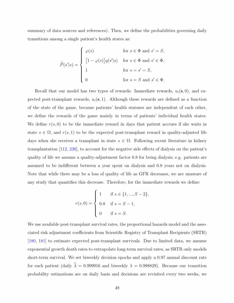
summary of data sources and references). Then, we define the probabilities governing daily

transitions among a single patient’s health states as:

P (s′|s) =

ϕ(s) for s ∈ Φ and s′ = S,[1− ϕ(s)

]q(s′|s) for s ∈ Φ and s′ ∈ Φ,

1 for s = s′ = S,

0 for s = S and s′ ∈ Φ.

Recall that our model has two types of rewards: Immediate rewards, ui(s, 0), and ex-

pected post-transplant rewards, ui(s, 1). Although these rewards are defined as a function

of the state of the game, because patients’ health statuses are independent of each other,

we define the rewards of the game mainly in terms of patients’ individual health states.

We define r(s, 0) to be the immediate reward in days that patient accrues if she waits in

state s ∈ Ω, and r(s, 1) to be the expected post-transplant reward in quality-adjusted life

days when she receives a transplant in state s ∈ Ω. Following recent literature in kidney

transplantation [112, 230], to account for the negative side effects of dialysis on the patient’s

quality of life we assume a quality-adjustment factor 0.8 for being dialysis; e.g. patients are

assumed to be indifferent between a year spent on dialysis and 0.8 years not on dialysis.

Note that while there may be a loss of quality of life as GFR decreases, we are unaware of

any study that quantifies this decrease. Therefore, for the immediate rewards we define:

r(s, 0) =

1 if s ∈ 1, ..., S − 2,

0.8 if s = S − 1,

0 if s = S.

We use available post-transplant survival rates, the proportional hazards model and the asso-

ciated risk adjustment coefficients from Scientific Registry of Transplant Recipients (SRTR)

[180, 181] to estimate expected post-transplant survivals. Due to limited data, we assume

exponential growth death rates to extrapolate long-term survival rates, as SRTR only models

short-term survival. We set biweekly decision epochs and apply a 0.97 annual discount rate

for each patient (daily λ = 0.999916 and biweekly λ = 0.998829). Because our transition

probability estimations are on daily basis and decisions are revisited every two weeks, we

48

adjust the daily parameters to a biweekly basis. We denote the matrix that governs biweekly

GFR transitions by P = P14. We also define ψt(s) as the total expected discounted imme-

diate reward in quality-adjusted life days that will be accrued in the last 14− t days of the

current stage, and recursively calculate it as:

ψt(s) =

r(s, 0) + λ

∑s′∈Ω

P (s′|s)ψt+1(s′) for s ∈ Ω and t = 0, ..., 13,

0 for s ∈ Ω and t = 14.

After we discount the expected post-transplant rewards and specify them by a subscript for

Patient i, we define the rewards of the game as follows:

ui(s,m) =

ri(si, 1) for s = (s1, s2) ∈ S \D and m = 1,

0 for s = (s1, s2) ∈ D and m = 1,

ψ0i (si) for s = (s1, s2) ∈ S and m = 0.

For our experiments, we simulate 2500 exchange cases by using the 10-year average frequency

of patient-donor characteristics in living-donor kidney transplantations that are available

from SRTR for the years 1998-2007. Following the proportional hazards model that we use

to estimate the expected post-transplant rewards, our simulations consider donor’s age and

gender; patient’s age, gender and race, and the antigen mismatch status between patient-

donor pairs as independent risk factors on patients’ expected post-transplant survivals. We

assume that patients are of same ethnicity with their incompatible donors, and unrelated

to the donor in the exchange who is compatible with her. We simulate the patients’ initial

GFR ranges uniformly over Φ.

49

3.3.2 Welfare Loss Due to Patient Autonomy and Equilibrium Selection

We solve our MIP models to characterize socially optimal mixed and pure equilibria. Through-

out the rest of this section, we let a socially optimal mixed (pure) equilibrium refer to the

equilibrium that maximizes the sum of the patients expected payoffs over the space of mixed

(pure) equilibria starting from the initial state of the game. For each case we solve the

mathematical programs

max(w,x,y)∈Λ

(∑i∈N

wi(s)

)and max

(w,x,y)∈Υ

(∑i∈N

wi(s)

),

to estimate the cost of restricting our attention to pure strategies in terms of the total number

of expected quality-adjusted life days. Note that because Υ ⊆ Λ, (i.e., the MIP that allows

randomized equilibria is a relaxation of the MIP that considers only pure equilibria), these

mathematical programs may share the same optimal solution. By Theorems 3.2 and 3.3,

max(w,x,y)∈Λ

[∑i∈N wi(s)

]− max(w,x,y)∈Υ

[∑i∈N wi(s)

]quantifies the aforementioned cost

exactly. Our experiments reveal that a socially optimal pure equilibrium is only negligibly

worse than a socially randomized optimal equilibrium. In all our instances, it is no more

than 0.01%. Therefore, as randomized strategies are less applicable than pure strategies,

we narrow our focus to pure equilibria and quantify the social welfare loss borne by patient

autonomy. In the rest of this section, we let A∗ refer to a socially optimal pure equilibrium.

We consider a central decision-maker who acts on behalf of both pairs for the society’s

interest. Provided that transplantation surgeries occur simultaneously and λ ∈ (0, 1) is the

social discount factor, the socially optimal policy from this decision-maker’s perspective may

be modeled as a discrete-time infinite horizon MDP. We assume this decision-maker revisits

her decisions periodically at the same frequency that the patients do in the game. We define

W (s) as the maximum total expected reward that the whole exchange cycle can gain in this

model when the system starts in state s ∈ S which we recursively calculate as:

W (s) = max

∑i∈N

ui(s, 1),∑i∈N

ui(s, 0) + λ∑s′∈S

P(s′|s)W (s′)

for s ∈ S . (3.46)

We let X denote the set of states in which exchange is an optimal decision in this model,

i.e., X =s ∈ S |W (s) =

∑i∈N ui(s, 1)

, and define ϑi(s) as the expected survival of

50

Patient i ∈ N starting in state s ∈ S under a socially optimal policy, which we recursively

calculate as follows:

ϑi(s) =

ui(s, 1) for s ∈X ,

Fi(s,ϑi) otherwise.(3.47)

Because A∗ is a socially optimal pure equilibrium, gi(s, a∗i , a∗−i)−ϑi(s) denotes the welfare

loss for Patient i ∈ N , and∑

i∈N[gi(s, a

∗i , a∗−i)− ϑi(s)

]denotes the minimum social welfare

loss due to patient autonomy. Note that the socially optimal policy may not be an equilibrium

of game G. In our experiments, we set λ = 0.998829.

15.3 13.7 8.5 -1.8 -10.4-30.7

-54.4-56.2 -57.8

16

19.7 25.9 3550.8

72

112.6

167.4

192

199.1

32.2 35 39.5 43.549 61.6

81.9

112.9 126.8141.3

-10

0

10

20

30

40

50

0 1 2 3 4 5 6 7 8 9

Difference in Patients' GFR ranges

Healthier Patient

Sicker Patient

Total

Welfare Loss (%)

Figure 3.2: Social welfare loss and patients’ individual welfare losses due to patient autonomy.

We treat the difference in the patients’ GFR ranges in the initial state of the game

(|s1− s2|) as a measure of conflict between their self-interests. We also consider the patients

seperately as healthier and sicker. Because lower GFR levels which indicate sicker conditions

are represented by higher state indices, Patient i refers to sicker patient if si ≥ s−i, and

healthier patient otherwise. For each case, we calculate the minimum social welfare loss and

51

the patients’ individual welfare losses in absolute (in quality-adjusted life-weeks) and relative

terms as a function of the difference in their GFR ranges. We present the average welfare

losses across our numerical experiments in Figure 3.2. In the figure, the number next to each

data label indicates the loss in quality-adjusted life weeks.

From the figure, social welfare loss does not decrease as the patients’ health statuses

diverge, which we interpret as follows: Because the central decision-maker acts solely for the

society’s interest and the death of one patient leaves the other untransplanted, as one of the

patients gets sicker, the central decision-maker becomes more likely to recommend exchange

as an optimal decision. On the other hand, when patients are autonomous, the healthier

patient can force the sicker patient to wait, although the sicker patient’s death would render

the exchange infeasible. Also, the sicker patient benefits from the central decision-maker’s

decisions, and the impact of patient autonomy on her welfare is more dramatic in absolute

and relative terms.

As the society’s interest may conflict with patients’ self-interests, a socially optimal

equilibrium strategy may not be an optimal equilibrium strategy that a patient can play.

Therefore, for each individual patient we calculate the cost of playing the socially optimal

equilibrium strategy rather than any other equilibrium strategy. We let iA∗ = (ia∗1,i a∗2)

denote a pure equilibrium that maximizes Patient i’s total expected payoff, i.e., iA∗ ∈

arg maxA∈Π gi(s, a1, a2). Then, gi(s,i a∗1,

i a∗2)− gi(s, a∗1, a∗2) provides an upper bound for Pa-

tient i’s cost of playing a socially optimal equilibrium strategy rather than any other equi-

librium strategy. For each Patient i ∈ N , by Theorem 3.3 (iii), we calculate gi(s,i a∗1,

i a∗2)

by solving the mathematical program max(w,y,z)∈Υwi(s).

From Table 3.2, as patients’ health statuses diverge, a socially optimal equilibrium consid-

ers the sicker patient’s interests more, that is, playing a socially optimal equilibrium strategy

costs less to the sicker patient. Irrespective of the difference in patients’ GFR ranges, a so-

cially optimal equilibrium deviates more from the healthier patient’s individually optimal

equilibrium than it does from the sicker’s. In our experiments, the sicker patient under

the socially optimal equilibrium is usually very close to her individually optimal equilib-

rium. Specifically, in 72% of the cases, the sicker patient’s individually optimal equilibrium

52

Table 3.2: Patients’ maximum welfare losses from following a socially optimal equilibrium.

Difference in Patients’ GFR Ranges

Loss Patient 0 1 2 3 4 5 6 7 8 9

RelativeHealthier 0.76 1.20 1.49 2.11 2.40 3.00 3.54 3.61 3.78 3.82

Sicker 0.89 0.80 0.71 0.68 0.61 0.58 0.57 0.50 0.26 0.00

AbsoluteHealthier 7.43 9.69 12.20 17.08 19.64 24.96 29.73 26.88 28.64 31.13

Sicker 7.43 6.57 5.75 5.28 6.04 4.15 3.41 2.67 1.26 0.00

Relative losses are in % and absolute losses are in quality-adjusted life weeks.

is within 1% of the socially optimal equilibrium, and in 90% of the cases her individually

optimal equilibrium is within 3% of the socially optimal equilibrium.

3.3.3 Valuing Exchanges: An Example

In this section, we elucidate how the patients’ quality-adjusted life expectancies from

our model can be used to calibrate edge-weights in graphs used to form patient-donor pairs.

We create an example graph of patient-donor pairs for which maximizing the total number

of transplants may imply adverse welfare outcomes. In Figure 3.3, we have 4 patient-donor

pairs with specified characteristics.

For the set of patient-donor pairs in Figure 3.3, we have two possible matching

scenarios: In Scenario 1, Patient 1 is matched to Donor 2, Patient 2 is matched to Donor

1, Patient 3 is matched to Donor 4, and Patient 4 is matched to Donor 3. In Scenario 2,

Patient 2 is matched to Donor 3, Patient 3 is matched to Donor 2, and Patients 1 and 4

remain untransplanted. Although Scenario 1 maximizes the number of transplants, when we

compare the social outcomes under such scenarios, we observe the following: In Scenario 1, an

immediate exchange yields a total of 53.27 QALYs. When the patients behave autonomously

in each of the matchings, the socially optimal equilibria yields 50.49 QALYs in total. In

53

P2

D2 D3

D1 D4

P3

P1 P4

Age = 50

Age = 65

Age = 55

Age = 50

0 ABDR mismatchnon-0 ABDR, 2DR mismatch

Female, Age = 45, GFR = 60 Male, Age = 50, GFR = 50

Male, Age = 70, GFR = 16 Female, Age = 65, GFR = 20

Figure 3.3: Patient-donor characteristics for the matching example

Scenario 2, an immediate exchange yields 52.76 QALYs. Because Patients 1 and 4 are

untransplanted, when Patients 2 and 3 behave autonomously, a socially optimal equilibria

yield 54.27 QALYs. Note that in this case, because we assume Patients 1 and 4 will never

receive a transplant, we calculate their remaining life expectancies by two separate Markov

reward chains(see d1 as an example in the proof of Theorem 3.3 (iv)

). Thus, if the patients

are autonomous and the edge weight of each possible matching is modeled as the patients’

total life expectancies in a socially optimal equilibrium of the game played in that particular

matching, then Scenario 2 is optimal although it has fewer transplants than Scenario 1.

Note that in Scenario 2, the socially optimal equilibrium provides considerably higher social

welfare than that of immediate exchange. Intuitively, when patients behave autonomously, if

they are at closer stages of disease, because they conflict less, their matchings yield superior

welfare outcomes compared to matchings involving patients at different stages.

54

3.4 CONCLUSIONS

Kidney exchanges have been formulated as finding matchings in a graph, the timing of ex-

change has not been addressed yet. In this chapter, we propose a weighting scheme to

value kidney exchanges for self-interested and autonomous patients with dynamic health.

We model the patients’ transplant timing decisions as a non-zero-sum stochastic game and

analyze the resulting equilibria of the game. Because a complete characterization of the

equilibria is computationally intractable, we develop mathematical programming represen-

tations of the resulting equilibrium conditions and analyze the equilibrium selection problem

from a societal point of view. The MIP formulation that we develop for pure equilibrium

selection can be easily extended to the multi-pair cyclic kidney exchanges such as 3- and

4-way kidney exhanges. Our numerical experiments indicate that matching patients based

on 0-1 preferences ignoring the timing of the exchange under patient autonomy may result in

socially suboptimal circumstances. We assess the importance of disease progression in timing

of an exchange and demonstrate that matching patients at similar stages of CKD provides

more preferable outcomes in terms of the social welfare gained by matching patients based

on their life expectancies and the social welfare lost by patient autonomy. Because patients

may exchange their kidneys prior to initiation of dialysis, our model and results also shed

light on the welfare consequences of preemptive PKEs which are recommended but not very

common in practice.

55

4.0 THE OPTIMAL TIMING OF STATIN INITIATION FOR PATIENTS

WITH TYPE 2 DIABETES

In this chapter we consider the question of when to initiate statin treatment to maximize

a Type 2 diabetes patient’s expected QALYs prior to the occurrence of the first CHD or

stroke event, or death from all other causes. We refer to these three outcomes collectively as

terminal events. Prevention of cardiovascular events is one of the primary goals of the ATP

III guidelines and the goal of maximizing QALYs prior to a first terminal event is consistent

with this goal.

We summarize the contributions of this chapter as follows. First, we develop a model

that can guide physicians and patients in the use of statins for the primary prevention of

cardiovascular events. Specifically, we formulate the statin initiation problem as a discrete-

time infinite-horizon MDP. We derive sufficient conditions for the resulting optimal policy

to be of control-limit type, and analyze how these limits change with respect to patient’s

age. Second, we present numerical results based on a large longitudinal data set from the

Mayo Clinic in Rochester, MN. Finally, we compare the performance of the published U.S.

guidelines to the optimal policies generated by our model.

The remainder of this chapter is organized as follows: In Section 4.1, we describe our

MDP model in detail. In Section 4.2 we analyze the structure of the underlying optimal

policies of our model. In Section 4.3 we support our analytical results by a series of numerical

experiments and present several policy implications. In Section 4.4 we present conclusions

and summarize the limitations of our model and numerical experiments.

56

4.1 MODEL FORMULATION

In this section, we formulate a discrete-time, infinite-horizon MDP model for the optimal

timing of statin initiation for patients with Type 2 diabetes. Once a patient with Type

2 diabetes initiates statin treatment, for the long-term benefit of the treatment, clinical

guidelines recommend that she should take statins for the remainder of her life [192, 222].

Assuming there are no severe side effects of the therapy, if we consider the clinical intent

for those patients who can tolerate the treatment, we can view statin initiation as a one-

time irreversible decision [192]. Therefore, the decision we consider is when to initiate statin

treatment over the course of the patient’s lifetime based on her CHD and stroke risk profile.

The objective of the MDP model is to maximize the patient’s QALYs prior to the first

terminal event.

Following the UKPDS risk model, we describe the patient’s CHD and stroke risk profile

by her cholesterol, SBP, HbA1c, age, gender, ethnicity and smoking status at diagnosis.

Of these risk factors, patient’s age, cholesterol, SBP and HbA1c levels are dynamic. We

incorporate the effect of the patient’s age on the CHD and stroke risk profile by a time

index. Consistent with other studies in the medical literature, we model the evolution of the

patient’s SBP and HbA1c levels deterministically as a function of time [29, 30, 87, 99, 105].

We model the progression of the patient’s on- and off-treatment LR levels stochastically

as a finite-state discrete-time Markov chain. We describe the components of our MDP model

in detail as follows:

Time Horizon : We assume the treatment decision is revisited periodically (e.g. annual

visits to an endocrinologist) over the patient’s lifetime prior to the occurrence of the first

terminal event. Because the time to first terminal event is random, our model has two

separate but back to back decision horizons as non-stationary and stationary (See Figure 4.1

for the division of the decision horizon into two subhorizons). The non-stationary decision

horizon is finite and precedes the stationary decision horizon. On the other hand, stationary

decision horizon is infinite long. We define T = 0, 1, 2, ..., N as the set of decision epochs,

where T ′ = T \ N represents the set of epochs in the non-stationary horizon. We assume

the problem parameters at epoch N − 1 remain stationary beyond epoch N − 1. Therefore,

57

epochs beyond N − 1 are not differentiated from each other and are represented by N .

This division and modeling of the decision horizon reflect the non-stationary nature of risk

with respect to age, and provides an approximation framework for the patient’s remaining

expected QALYs prior to the first terminal event over the time horizon for which there is

insufficient medical data due to low sample sizes at high ages. Finally, we let stage t refer

to time interval between epochs t and t + 1 and without loss of generality, we assume the

length of each stage is τ > 0 years.

States : We discretize the continuous range of LR values by a finite set of states L′ =

1, 2, ..., L where each ` ∈ L′ corresponds to a pre-specified LR-range and lower indexed

ranges indicate lower values of LR. We add an absorbing state L+ 1 to the set of LR-ranges

to denote a terminal event, and let L = L′ ∪ L + 1. Note that our state description also

involves static risk factors, including age, gender, smoking status, and dynamic but non-

stochastic risk factors: SBP, HbA1C. Because these factors are not affected by the patient’s

treatment status in our model, for notational convenience we suppress the dependency on

them.

Actions : In each state ` ∈ L there are two possible actions and the action is chosen from

the set W, I, where W represents waiting for one more stage and I stands for initiating

treatment immediately. We assume that using statins reduces the patient’s LR level by a

factor ω which we call the patient’s treatment-effect factor. We define the treatment status

of the patient by a binary indicator m ∈ M = 0, 1, where “0” and “1” refer to not using

and using statins, respectively. Because statin initiation is a one-time irreversible decision,

once treatment is initiated m switches from 0 to 1 and remains as such.

Probabilities : We have four types of probabilities in our model: The probabilities of non-

CHD or stroke-related death, CHD and stroke probabilities, and the transition probabilities

among the LR-ranges. At epoch t ∈ T ′, a non-CHD or stroke-related death occurs with

probability dt. Otherwise, if the patient is in state ` ∈ L′ under treatment status m ∈ M,

a CHD event occurs with probability πCt (`,m) and a stroke event occurs with probability

πSt (`,m) (See Section 4.3.2 for details on how we estimate CHD and stroke probabilities).

Assuming that CHD and stroke events are mutually exclusive, i.e. they do not occur simul-

taneously at the same time in any particular stage, we let π5t (`,m) = πCt (`,m) + πSt (`,m)

58

denote the patient’s probability of having a CHD or a stroke event in state ` ∈ L′ under

treatment status m ∈M in stage t.

Given the patient is in state ` ∈ L under treatment status m ∈ M at epoch t ∈ T ′, the

probability of moving into the absorbing state L+1 at epoch t+1 is denoted by pmt (L+1|`),

where pmt (L + 1|`) = dt + [1 − dt]π5t (`,m) for (`,m) ∈ L′ ×M and pmt (L + 1|L + 1) = 1

for both m ∈ M. Given the patient is in state ` ∈ L′ at epoch t ∈ T ′ and does not incur

a terminal event in stage t, the probability of being in state `′ ∈ L′ at the next epoch is

denoted by q(`′|`). Note that probabilities q(`′|`) are conditional on patient’s survival from

a terminal event. Then, we define pmt (`′|`) to be the patient’s probability of being in state

`′ ∈ L at epoch t + 1 given she is in state ` ∈ L under treatment status m ∈ M at epoch

t ∈ T ′, which we write as:

pmt (`′|`) =

[1− pmt (L+ 1|`)

]q(`′|`) if `, `′ ∈ L′,

pmt (L+ 1|`) if ` ∈ L′, `′ = L+ 1,

1 if ` = `′ = L+ 1,

0 otherwise.

(4.1)

For convenience we let Q = [q(`′|`)] denote the patient’s conditional LR-range transition

probability matrix and Pm(t) = [pmt (`′|`)] denote the patient’s unconditional transition prob-

ability matrix under treatment status m ∈M at epoch t ∈ T ′.

Rewards : Studies on statin treatment incorporate the health-related quality of life adjust-

ment due to negative side effects of statins by means of a disutility coefficient [155, 212]. We

define rm(`) = τ(1 − mσ) to be the immediate reward in QALYs accrued in state ` ∈ L′,

under treatment status m ∈ M, where the parameter σ ∈ [0, 1] is referred to as the utility

decrement or disutility and represents the reduction in quality of life during a year of life due

to side effects from medication. Since our objective is to maximize the patient’s QALYs prior

to the first terminal event, we set all the immediate rewards associated with the absorbing

state L + 1 to zero, i.e., rm(L + 1) = 0 for both m ∈ M. Figure 4.2 illustrates the states,

transitions and rewards for a particular stage t. The single node on the left represents the

patient’s current LR-range at epoch t. The nodes on the right are partitioned into states as

LR-ranges and terminal events.

59

Figure 4.1: Division of the decision horizon into non-stationary and stationary subhorizons.

Pm(t) denotes the probability matrix that governs the transitions in stage t ∈ T for m = 0 (off-treatment)and m = 1 (on-treatment).

For notational convenience, in the rest of this chapter, except the transition probability

matrices, we let the terms in bold refer to a real-valued L+1 dimensional vector, i.e., v refers

to the vector[v(`)

]`∈L. For convenience, given v ∈ RL+1, ` ∈ L, m ∈ 0, 1 and t ∈ T ′,

we define Fmt (`,v) = λ

∑`′∈L p

mt (`′|`)v(`′). We also represent componentwise operations and

relations between two vectors in vector notation. For instance, given v1 =[v1(`)

]`∈L and

v2 =[v2(`)

]`∈L, v1 = v2 refers to v1(`) = v2(`) for all ` ∈ L.

In our model, the patient continues to accumulate rewards prior to her first CHD or

stroke event. Once she incurs a terminal event she transitions into state L + 1, which is

absorbing and provides no rewards. Therefore, upon occurrence of a terminal event, the

accumulation of rewards stops and the patient terminates the process. We define µt(`) as

the patient’s expected post-treatment reward if the treatment is initiated in state ` ∈ L at

epoch t ∈ T . Since statin initiation is a one-time decision and the patient uses statins from

the time of initiation to the end of her life, the expected post-treatment rewards can be

60

Figure 4.2: State transition diagram at epoch t ∈ T ′ under treatment status m ∈M.

recursively defined as:

µt(`) =

r1(`) + F 1t (`,µt+1) for ` ∈ L and t ∈ T ′,

r1(`) + F 1t−1(`,µt) for ` ∈ L and t = N ;

(4.2)

where λ ∈ (0, 1) is the discount factor per stage [59, 82].

For a patient with no history of CHD or stroke in state ` ∈ L at epoch t ∈ T , we let

ut(`) denote the maximum total expected discounted QALYs prior to the first terminal event

and we define at(`) as the corresponding optimal action, which we determine by solving the

following optimality equations:

ut(`) =

max r0(`) + F 0t (`,ut+1), µt(`) for ` ∈ L and t ∈ T ′,

maxr0(`) + F 0

t−1(`,ut), µt(`)

for ` ∈ L and t = N .(4.3)

Specifically, in state ` ∈ L of epoch t ∈ T , if ut(`) = µt(`), then it is optimal to initiate

treatment, i.e. at(`) = I. Otherwise, it is optimal to wait, i.e. at(`) = W . Note that the

61

expected post-treatment rewards in (4.3) are determined by a separate Markov reward chain

in which the patient is on statins. Therefore, they are fixed composite parameters of the

model.

4.2 STRUCTURAL PROPERTIES

In this section we derive structural results of the MDP model that we developed in section

4.1. While MDP models have been applied in several other clinical contexts (for an extensive

review of discrete-time Markov models in health care see [9, 10, 52, 125, 176]), we provide sev-

eral extensions. Specifically, within the context of living-donor liver transplantation, Alagoz

et al. [10] provides sufficient conditions to prove the existence of an optimal control-limit

policy for an infinite-horizon optimal stopping time model. Although reasonable for liver

transplant decisions this assumption is not appropriate for long-term chronic diseases, such

as diabetes and heart disease, for which the risk of complications and comorbidities changes

significantly with age [31]. We provide weaker and more intuitive conditions to establish the

optimality of control-limit policies in both stationary and non-stationary contexts. Since

most U.S. guidelines do not acknowledge age as an explicit risk factor in treating patients

with diabetes we also analyze the time-behavior of the resulting control-limits to investigate

the influence of age in treatment design.

We begin our analyses by defining the notion of an “increasing failure rate” (IFR) tran-

sition probability matrix, which has been shown to be useful in proving the structural prop-

erties of MDPs in maintenance and reliability theory and appears to match clinical data

closely in varying contexts [10, 109, 219].

Definition 4.1. [21] An n × n stochastic matrix H =[h(j|i)

]is said to have the IFR

property if∑k

j=1 h(j|i) is nonincreasing in i for all k = 1, ..., n.

In our model, under treatment status m ∈ M at epoch t ∈ T ′, if the matrix Pm(t) is

IFR, an intuitive explanation is as follows: The higher the LR the patient has at epoch t

under treatment status m, the more likely she is to have a higher LR or to incur a terminal

62

event at epoch t+1. By Proposition 4.1, given the patient’s on- and off-treatment transition

probabilities have the IFR property at each epoch, the maximum expected QALYs prior to

the first terminal event does not increase in LR.

Proposition 4.1. If Pm(t) is IFR for all m ∈ M and t ∈ T ′, then the optimal value

function, ut(`), is nonincreasing in ` ∈ L for all t ∈ T .

Proof. Because P1(N − 1) is IFR for all t ∈ T ′ and r1(`) is nonincreasing in ` ∈ L, by

the infinite-horizon extension of Theorem 4.7.3 of Puterman [161], µN(`) is nonincreasing in

` ∈ L. Then, because P1(t) is IFR for all t ∈ T ′, Theorem 4.7.3 of Puterman [161] itself

implies that µt(`) is nonincreasing in ` ∈ L for all t ∈ T ′. Because r0(`) is nonincreasing in

` ∈ L and µt(`) is nonincreasing in ` ∈ L for all t ∈ T , the proof of the monotonicity of ut(`)

is similar by applying Theorem 4.7.3 of Puterman [161] and its infinite-horizon extension.

Next, we define an expected benefit loss function which we use to express our main

theoretical results. We let Bt(`) denote the patient’s expected benefit loss in QALYs from

delaying the initiation of treatment to the next epoch in LR-range ` ∈ L of epoch t ∈ T ′,

and define it as Bt(`) = µt(`)− F 0t (`,µt+1).

In our problem context, we define a control-limit policy as follows: A patient should initi-

ate treatment if and only if her LR is above some threshold. Note that many published lipid

management guidelines, including well known U.S. guidelines, have a control-limit structure

depending on the risk factors they use to define the patient’s risk profile. Theorem 4.1 pro-

vides sufficient conditions for the existence of an optimal control-limit policy. Specifically,

it relates the existence of such a policy to the IFR property of the off-treatment transition

probability matrices and the monotonicity of the expected benefit loss function. Intuitively

a non-decreasing benefit loss with respect to age and LR can be interpreted to mean the

benefit of delaying the initiation of treatment does not get smaller as patient gets older, or

as her health becomes worse.

Theorem 4.1. Suppose P0(t) is IFR for all t ∈ T ′ and Bt(`) is nondecreasing in ` ∈ L′ for

all t ∈ T ′. Then, there exists an LR threshold `∗t ∈ L′ for each t ∈ T such that the optimal

action in state ` at epoch t is to initiate treatment if and only if ` ≥ `∗t , i.e., at(`) = I for

all ` ≥ `∗t , and at(`) = W otherwise.

63

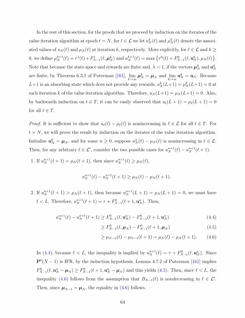
In the rest of this section, for the proofs that we proceed by induction on the iterates of the

value iteration algorithm at epoch t = N , for ` ∈ L we let ukN(`) and µkN(`) denote the associ-

ated values of uN(`) and µN(`) at iteration k, respectively. More explicitly, for ` ∈ L and k ≥

0, we define µk+1N (`) = r1(`) +F 1

N−1(`,µkN) and uk+1N (`) = max

r0(`) + F 0

N−1(`,ukN), µN(`)

.

Note that because the state space and rewards are finite and, λ < 1, if the vectors µ0N and u0

N

are finite, by Theorem 6.3.1 of Puterman [161], limk→∞

µkN = µN and limk→∞

ukN = uN . Because

L+1 is an absorbing state which does not provide any rewards, ukN(L+1) = µkN(L+1) = 0 at

each iteration k of the value iteration algorithm. Therefore, uN(L+1) = µN(L+1) = 0. Also,

by backwards induction on t ∈ T , it can be easily observed that ut(L + 1) = µt(L + 1) = 0

for all t ∈ T .

Proof. It is sufficient to show that ut(`) − µt(`) is nonincreasing in ` ∈ L for all t ∈ T . For

t = N , we will prove the result by induction on the iterates of the value iteration algorithm.

Initialize u0N = µN , and for some n ≥ 0, suppose unN(`) − µN(`) is nonincreasing in ` ∈ L.

Then, for any arbitrary ` ∈ L′, consider the two possible cases for un+1N (`)− un+1

N (`+ 1).

1. If un+1N (`+ 1) = µN(`+ 1), then since un+1

N (`) ≥ µN(`),

un+1N (`)− un+1

N (`+ 1) ≥ µN(`)− µN(`+ 1).

2. If un+1N (` + 1) > µN(` + 1), then because un+1

N (L + 1) = µN(L + 1) = 0, we must have

` < L. Therefore, un+1N (`+ 1) = τ + F 0

N−1(`+ 1,unN). Then,

un+1N (`)− un+1

N (`+ 1) ≥ F 0N−1(`,unN)− F 0

N−1(`+ 1,unN) (4.4)

≥ F 0N−1(`,µN)− F 0

N−1(`+ 1,µN) (4.5)

≥ µN−1(`)− µN−1(`+ 1) = µN(`)− µN(`+ 1). (4.6)

In (4.4), because ` < L, the inequality is implied by un+1N (`) = τ + F 0

N−1(`,unN). Since

P0(N − 1) is IFR, by the induction hypothesis, Lemma 4.7.2 of Puterman [161] implies

F 0N−1(`,unN −µN) ≥ F 0

N−1(`+ 1,unN −µN) and this yields (4.5). Then, since ` < L, the

inequality (4.6) follows from the assumption that BN−1(`) is nondecreasing in ` ∈ L′.

Then, since µN−1 = µN , the equality in (4.6) follows.

64

Thus, un+1N (`) − µN(`) is nonincreasing in ` ∈ L. Then, by induction, the convergence

of the algorithm implies that uN(`) − µN(`) is nonincreasing in ` ∈ L. The proof of the

monotonicity of ut(`)− µt(`) in ` ∈ L for t < N is similar by backwards induction on t and

omitted.

Next, we focus on how the optimal policy changes with respect to age. It is well established

that age is a positive risk factor for CHD and stroke. The mortality data published by the

National Center for Health Statistics (NCHS) also state that patient’s non-CHD or stroke-

related death probability increases by age [134]. Therefore, in the rest of this chapter, for our

analyses, we assume that dt is nondecreasing in t ∈ T ′. By the definition of the transition

probabilities, this assumption has the following implication:

pmt+1(L+ 1|`) ≥ pmt (L+ 1|`) for all ` ∈ L, m ∈M, t ∈ T ′ \ N − 1. (4.7)

Proposition 4.2 expresses the time-monotonicity of the patient’s value function.

Proposition 4.2. The optimal value function vector, ut, is nonincreasing in t ∈ T .

Proof. First, by backwards induction on t ∈ T , we will show that µt is nonincreasing in t ∈ T .

By definition, we have µN−1 = µN . For some k + 1 < N − 1, assume that µk+1 ≥ µk+2.

Then, for an arbitrary ` ∈ L′:

µk(`)− µk+1(`) = F 1k (`,µk+1)− F 1

k+1(`,µk+2) ≥ F 1k+1(`,µk+1 − µk+2) ≥ 0. (4.8)

Since p1k+1(L + 1|`) ≥ p1

k(L + 1|`), by definition, p1k(`′|`) ≥ p1

k+1(`′|`) for all `′ ∈ L′ and

the first inequality in (4.8) follows. Then, the second inequality in (4.8) follows from the

induction hypothesis. Hence, µk ≥ µk+1, and by induction µt is nonincreasing in t ∈ T .

Using the time-monotonicity of µt, the proof of the monotonicity of ut in t ∈ T is similar to

that of µt by backwards induction on t and omitted.

According to Proposition 4.2, the optimal value function does not increase with age; that is,

the patient’s expected QALYs prior to the first terminal event do not increase as she ages.

Theorem 4.2 defines the structure of the optimal policy with respect to age.

65

Theorem 4.2. If Bt is nondecreasing in t ∈ T ′, then for any ` ∈ L and t ∈ T ′, at(`) = I

implies at+1(`) = I.

Proof. It is sufficient to show that ut(`)−µt(`) is nonincreasing in t ∈ T for all ` ∈ L, which

we will prove by backwards induction on t. By definition, µN−1 = µN and uN−1 = uN .

Therefore, uN − µN = uN−1 − µN−1. As the induction hypothesis, for some k + 1 < N ,

suppose uk+1 − µk+1 ≥ uk+2 − µk+2. Now, for fixed ` ∈ L consider the possible cases for

uk(`)− uk+1(`).

1. If uk+1(`) = µk+1(`), then because uk(`) ≥ µk(`),

uk(`)− uk+1(`) ≥ µk(`)− µk+1(`).

2. If uk+1(`) > µk+1(`), then

uk(`)− uk+1(`) ≥ F 0k (`,uk+1)− F 0

k+1(`,uk+2) (4.9)

≥ F 0k+1(`,uk+1 − uk+2) ≥ F 0

k+1(`,µk+1 − µk+2), (4.10)

where (4.9) is implied by uk(`) = r0(`) + F 0k (`,uk+1). Since p0

k+1(L+ 1|`) ≥ p0k(L+ 1|`),

by definition, p0k(`′|`) ≥ p0

k+1(`′|`) for all `′ ∈ L′, and this yields the first inequality in

(4.10). Then, the second inequality in (4.10) is implied by the induction hypothesis.

Since Bk+1(`) ≥ Bk(`), (4.10) implies uk(`)− uk+1(`) ≥ µk(`)− µk+1(`).

Thus, uk − µk ≥ uk+1 − µk+1, and the result follows by induction on t.

Theorem 4.2 states that if the patient’s expected benefit loss from delaying the initiation

of treatment to the next epoch does not decrease over time then the patient becomes more

likely to initiate treatment at the same LR level as she ages. Therefore, if there exists an

optimal control-limit policy, the thresholds for treatment do not increase and the patient

maintains tighter control of her LR to avoid treatment as she ages.

In the remainder of this section, we will explore the sensitivity of the patient’s optimal

value function and policy with respect to quality-adjustment and treatment-effect factors.

To this end, Proposition 4.3 compares two patients who are identical except for their quality-

adjustment and/or treatment-effect factors. The relationship between treatment design and

66

patient’s response to treatment has been widely discussed in the medical literature [240].

Proposition 4.3 formalizes this relationship by stating that if it is optimal to initiate treat-

ment at a given LR level, it must be optimal to do so at the same level as the patient’s

disutility of using statins decreases, and/or the treatment effect factor increases.

In the rest of the chapter, when we compare two patients, for Patient i = 1, 2, we specify

the problem parameters, the value functions and the optimal actions by a pre-superscript,

i = 1, 2.

Proposition 4.3. Consider two patients who are identical except 2σ ≥ 1σ and/or 1ω ≥ 2ω.

Then, for any ` ∈ L and t ∈ T , 2at(`) = I implies 1at(`) = I.

Proof. Note that if we consider m continuous, 0 ≤ m ≤ 1, because ω < 1, it can be easily

shown that∂πCt (`,m)

∂mand

∂πSt (`,m)

∂mare both nonpositive for all ` ∈ L′

(See section 4.3.2

for the mathematical definition of the CHD and stroke probabilities, πCt (`,m) and πSt (`,m)).

Then, by definition (4.1), it is easy to see that p0t (`′|`) ≤ p1

t (`′|`) for all `, `′ ∈ L′ and t ∈ T ′.

Also, given two patients with quality-adjustment factors 1σ ≤ 2σ, if 1p1t (`′|`) ≥ 2p1

t (`′|`) for

`, `′ ∈ L′ and t ∈ T ′, then it is straightforward to show that 1µt ≥ 2µt for all t ∈ T .

First, we will establish an auxiliary result. Given two patients with 1σ ≤ 2σ, if

1p0t (`′|`) ≤ 2p0

t (`′|`), and 1p1

t (`′|`) ≥ 2p1

t (`′|`) for all `, `′ ∈ L′ and t ∈ T ′, (4.11)

then for any ` ∈ L and t ∈ T , 2at(`) = I implies 1at(`) = I. To prove the claim, it is

sufficient to show that 1ut − 1µt ≤ 2ut − 2µt for all t ∈ T . To establish this result for

t = N , we will proceed by induction on the iterates of the value iteration algorithm. We

will apply the algorithm to iuN simultaneously for both i = 1, 2. By the convergence of the

algorithm it is sufficient to show that 1ukN − 1µN ≤ 2ukN − 2µN for all k ≥ 0. Initialize

iu0N = iµN for i = 1, 2 and for some n ≥ 0, suppose 1unN − 1µN ≤ 2unN − 2µN . Now, for

an arbitrary ` ∈ L consider the possible cases for 2un+1N (`)− 1un+1

N (`).

1. If 1un+1N (`) = 1µN(`), then because 2un+1

N (`) ≥ 2µN(`),

2un+1N (`)− 1un+1

N (`) ≥ 2µN(`)− 1µN(`).

67

2. If 1un+1N (`) > 1µN(`), then

2un+1N (`)− 1un+1

N (`) ≥ 2F 0N−1(`, 2unN)− 1F 0

N−1(`, 1unN) (4.12)

= 2F 0N−1(`, 2unN − 2µN) + 2F 0

N−1(`, 2µN)

− 1F 0N−1(`, 1unN − 1µN)− 1F 0

N−1(`, 1µN) (4.13)

≥ 2F 0N−1(`,1 unN − 1µN)− 1F 0

N−1(`,1 unN − 1µN) + 2F 0N−1(`, 2µN)

− 1F 0N−1(`, 1µN) (4.14)

≥ 2F 0N−1(`, 2µN)− 1F 0

N−1(`, 1µN) (4.15)

≥ 2F 1N−1(`, 2µN)− 1F 1

N−1(`, 1µN) + τ(1σ − 2σ) = 2µN(`)− 1µN(`), (4.16)

where (4.12) follows from the fact that 2un+1N (`) ≥ r0(`) + 2F 0

N−1(`, 2unN). Then, (4.13)

is by adding and subtracting 1F 0N−1(`, 1µN) and 2F 0

N−1(`, 2µN) and (4.14) is implied

by the induction hypothesis. Since 2p0N−1(`′|`) ≥ 1p0

N−1(`′|`) for all `′ ∈ L′, 1unN ≥ 1µN

and 1unN(L + 1) = 1µN(L + 1) = 0, (4.15) is implied by 2F 0N−1(`, 1unN − 1µN) ≥

1F 0N−1(`, 1unN − 1µN). Finally, we show the inequality in (4.16) as follows: By (4.11),

1p1N−1(`′|`) − 1p0

N−1(`′|`) ≥ 2p1N−1(`′|`) − 2p0

N−1(`′|`) for all `′ ∈ L′. Also, because

1σ ≤ 2σ and (4.11) holds, 1µN ≥ 2µN . Then, since iµN(L + 1) = 0 for both i = 1, 2,

1F 1N−1(`, 1µN)− 1F 0

N−1(`, 1µN) ≥ 2F 1N−1(`, 2µN)− 2F 0

N−1(`, 2µN). By the fact that

1σ ≤ 2σ, this yields the inequality in (4.16).

Thus, 1un+1N − 1µN ≤ 2un+1

N − 2µN , and by the convergence of the algorithm the result

for t = N follows by induction on n. Then the proof of the fact that 1ut− 1µt ≤ 2ut− 2µt

for t ∈ T is similar by backwards induction on t, and omitted.

Now, we will treat each “or” case separately. We will omit the proof of the “and” case

since it is similar. If the patients are identical except 1σ ≤ 2σ, then the result directly follows

from the auxiliary result that has been shown above. Otherwise, if the patients are identical

except 1ω ≥ 2ω, by (4.43a)-(4.44c), 1π5t (`, 0) = 2π5t (`, 0) and 1π5t (`, 1) ≤ 2π5t (`, 1) for

all ` ∈ L′ and t ∈ T ′. Then, since 1Q = 2Q and 1dt = 2dt for all t ∈ T ′, by definition (4.1),

we have 1p1t (`′|`) ≥ 2p1

t (`′|`) and 1p0

t (`′|`) = 2p0

t (`′|`) for all `, `′ ∈ L′ and t ∈ T ′, and the

result follows from the auxiliary result that has been shown above.

68

Next, Proposition 4.4 establishes the sensitivity of the patient’s optimal value function

with respect to simultaneous changes in quality-adjustment and treatment-effect factors. It

states that the lower the quality-adjustment factor the patient has, the higher the benefit

she gains as the treatment-effect increases. Intuitively, by Proposition 4.3, as the quality-

adjustment factor decreases the patient uses statins more often by initiating therapy in a

wider set of states. Then, because the treatment reduces the patient’s CHD and stroke risks

in a more number of states, an increase in treatment-effect factor yields a greater increase

in patient’s QALYs prior to a terminal event.

Proposition 4.4. Consider two patients who are identical except 1ω ≥ 2ω. Let σ1 and σ2 be

two quality-adjustment factors with σ1 ≥ σ2, and let i,jut(`) specify iut(`) when the quality-

adjustment factor is σj, for ` ∈ L, t ∈ T and i, j = 1, 2. Then, 1,2ut − 1,1ut ≥ 2,2ut − 2,1ut

for all t ∈ T .

Proof. For brevity, we will establish the result only for t = N . Let i,jµN(`) denote the

expected post-treatment reward of patient i, i = 1, 2, in state ` ∈ L at epoch t = N when

her quality-adjustment factor is σj, j = 1, 2. First, we will show that 1,2µN − 1,1µN ≥2,2µN− 2,1µN . We will proceed by induction on the iterates of the value iteration algorithm.

We will apply the algorithm to 1,jµN for both j = 1, 2. Initialize 1,jµ0N = 2,jµN for j = 1, 2.

As the induction hypothesis, for some n ≥ 0, suppose 1,2µnN − 1,1µnN ≥ 2,2µN − 2,1µN .

Note that 1,2µn+1N (L + 1) = 1,1µn+1

N (L + 1) = 2,2µN(L + 1) = 2,1µN(L + 1) = 0. Then, for

an arbitrary ` ∈ L′,

1,2µn+1N (`)− 1,1µn+1

N (`)−[

2,2µN(`)− 2,1µN(`)]

= 1F 1N−1(`, 1,2µnN − 1,1µnN)− 2F 1

N−1(`, 2,2µN − 2,1µN)

≥ 1F 1N−1(`, 1,2µnN − 1,1µnN − 2,2µN + 2,1µN) ≥ 0. (4.17)

Because the patients are identical except 1ω ≥ 2ω:

1p1N−1(`′|`) ≥ 2p1

N−1(`′|`) and 1p0N−1(`′|`) = 2p0

N−1(`′|`) for all `, `′ ∈ L′. (4.18)

Now, because σ1 ≥ σ2, 2,2µN ≥ 2,1µN . Because 2,2µN(L + 1) = 2,1µN(L + 1) = 0, by

(4.18) this implies 1F 1N−1(`, 2,2µN − 2,1µN) ≥ 2F 1

N−1(`, 2,2µN − 2,1µN), yielding the

69

first inequality in (4.17). The second inequality in (4.17) directly follows from the induction

hypothesis. Thus, 1,2µn+1N − 1,1µn+1

N ≥ 2,2µN − 2,1µN . Then, by induction the convergence

of the algorithm yields

1,2µN − 1,1µN ≥ 2,2µN − 2,1µN . (4.19)

Next, for t = N , we will apply the value iteration algorithm simultaneously to i,juN for

i, j = 1, 2 to show that 1,2uN − 1,1uN ≥ 2,2uN − 2,1uN . We will proceed by induction on

the iterates of the algorithm. Initialize i,ju0N = i,jµN for i, j = 1, 2. By (4.19), this implies

1,2u0N − 1,1u0

N ≥ 2,2u0N − 2,1u0

N . As the induction hypothesis, for some n ≥ 0, suppose

1,2unN − 1,1unN ≥ 2,2unN − 2,1unN . We will make use of the following set of auxiliary results

to establish 1,2un+1N − 1,1un+1

N ≥ 2,2un+1N − 2,1un+1

N .

• Since σ1 ≥ σ2, by treating each patient as two identical patients with different quality-

adjustment factors we have,

i,1unN − i,1µN ≥ i,2unN − i,2µN for i = 1, 2. (4.20)

Similarly, since (4.18) is satisfied,

2,junN − 2,jµN ≥ 1,junN − 1,jµN for j = 1, 2. (4.21)

(The proofs of (4.20) and (4.21) are given in the proof of Proposition 4.3).

• Define i,jU(`) = r0(`) + iF 0N−1(`, i,junN) for ` ∈ L and i, j = 1, 2. For an arbitrary ` ∈ L,

consider 1,2U(`)− 1,1U(`)− [2,2U(`)− 2,1U(`)].

1,2U(`)− 1,1U(`)−[

2,2U(`)− 2,1U(`)]

= 1F 0N−1(`, 1,2unN − 1,1unN)− 2F 0

N−1(`, 2,2unN − 2,1unN) ≥ 0,

where the inequality is implied by the fact that 2p0N−1(`′|`) = 1p0

N−1(`′|`) for all `′ ∈ L

and the induction hypothesis. Thus,

1,2U− 1,1U ≥ 2,2U− 2,1U. (4.22)

70

• For fixed ` ∈ L, consider 1,2µN(`)− 2,2µN(`).

1,2µN(`)− 2,2µN(`) = 1F 1N−1(`, 1,2µN)− 2F 1

N−1(`, 2,2µN)

≥ 1F 0N−1(`, 1,2µN)− 2F 0

N−1(`, 2,2µN) (4.23)

≥ 1F 0N−1(`, 1,2unN)− 2F 0

N−1(`, 2,2unN) = 1,2U(`)− 2,2U(`). (4.24)

By the on-treatment transition probabilities in (4.18) it can be easily shown that 1,2µN ≥2,2µN . Also,

(by (4.18)

), because 1p1

N−1(`′|`)− 1p0N−1(`′|`) ≥ 2p1

N−1(`′|`)− 2p0N−1(`′|`) ≥

0 for all `′ ∈ L′ and 1,2µN(L+ 1) = 2,2µN(L+ 1) = 0,

1F 1N−1(`, 1,2µN)− 1F 0

N−1(`, 1,2µN) ≥ 2F 1N−1(`, 2,2µN)− 2F 0

N−1(`, 2,2µN),

and this yields (4.23). Then, the inequality in (4.24) is implied by 1F 0N−1(`, 1,2µN −

1,2unN) ≥ 2F 0N−1(`, 2,2µN− 2,2unN) which follows from (4.21) and the fact that 1p0

N−1(`′|`) =

2p0N−1(`′|`) for all `′ ∈ L. Thus,

1,2µN − 2,2µN ≥ 1,2U− 2,2U. (4.25)

Next, for an arbitrary ` ∈ L consider the possible cases for 1,2un+1N (`)− 2,2un+1

N (`). Note

that i,jun+1N (`) = max

i,jU(`),i,j µN(`)

for ` ∈ L and i, j = 1, 2.

1. If 1,1un+1N (`) = 1,1µN(`), then by (4.20), 1,2un+1

N (`) ≤ 1,2µN(`). By the definition of

1,2un+1N (`), we also have 1,2un+1

N (`) ≥ 1,2µN(`). These imply 1,2un+1N (`) = 1,2µN(`). Then,

1,2un+1N (`)− 1,1un+1

N (`)−[

2,2un+1N (`)− 2,1un+1

N (`)]

= 1,2µN(`)− 1,1µN(`)−[

2,2un+1N (`)− 2,1un+1

N (`)]

≥ 1,2µN(`)− 1,1µN(`)− 2,2µN(`) + 2,1µN(`) ≥ 0, (4.26)

where the first inequality in (4.26) is implied by (4.20) and the second inequality follows

from (4.19).

2. If 1,1un+1N (`) = 1,1U(`), then by (4.21), 2,1un+1

N (`) = 2,1U(`). Now, consider the possible

subcases:

71

a. If 2,2un+1N (`) = 2,2µN(`), then by (4.21), 1,2un+1

N (`) ≤ 1,2µN(`). By the definition of

1,2un+1N (`), we also have 1,2un+1

N (`) ≥ 1,2µN(`). These imply 1,2un+1N (`) = 1,2µN(`).

Then,

1,2un+1N (`)− 1,1un+1

N (`)−[

2,2un+1N (`)− 2,1un+1

N (`)]

= 1,2µN(`)− 1,1U(`)− 2,2µN(`) + 2,1U(`)

≥ 1,2U(`)− 1,1U(`)− 2,2U(`) + 2,1U(`) ≥ 0, (4.27)

where the first inequality in (4.27) is implied by (4.25) and the second inequality

follows from (4.22).

b. If 2,2un+1N (`) = 2,2UN(`), then because 1,2un+1

N (`) ≥ 1,2U(`), (4.22) implies

1,2un+1N (`)− 1,1un+1

N (`)−[

2,2un+1N (`)− 2,1un+1

N (`)]

≥ 1,2U(`)− 1,1U(`)−[

2,2U(`)− 2,1U(`)]≥ 0.

Thus, 1,2un+1N − 1,1un+1

N ≥ 2,2un+1N − 2,1un+1

N . Then, by induction, the convergence

of the algorithm yields 1,2uN − 1,1uN ≥ 2,2uN − 2,1uN . The proof of the fact that

1,2ut − 1,1ut ≥ 2,2ut − 2,1ut for t ∈ T ′ is similar by backwards induction on t ∈ T and

omitted.

Note that by Proposition 4.4, the patient’s optimal value function does not decrease as

σ decreases and/or ω increases.

Finally, we show that our conditions for Theorem 4.1 are less restrictive than those of

Alagoz et al. [10] which provides sufficient conditions to discover the existence of a threshold-

structured optimal policy for an infinite-horizon optimal stopping time model. In our model,

because the optimal policy remains stationary beyond epoch N−1, the optimality equations

72

at epoch N represent a similar infinite-horizon optimal stopping time model. The following

conditions are the equivalents of Alagoz et al. [10] in our context at epoch N .

PN−1(0) is IFR. (4.28)

r0(`) is nonincreasing in ` ∈ L′. (4.29)

µN(`) is nonincreasing in ` ∈ L′. (4.30)

L∑k=j

p0N−1(k|`) ≤

L∑k=j

p0N−1(k|`+ 1) for all j = `+ 1, ..., L and ` = L′ \ L. (4.31)

µN(`)− µN(`+ 1)

µN(`)≤ λ

[p0N−1(L+ 1|`+ 1)− p0

N−1(L+ 1|`)]

for ` = L′ \ L. (4.32)

By the definition of the immediate rewards, (4.29) holds immediately. By Theorem 4.1, to

have an LR-based optimal control-limit policy, in addition to (4.28), instead of (4.30)-(4.32)

we require the monotonicity of BN−1(`) with respect to ` ∈ L′. Next, we will show that it is

less restrictive than satisfying (4.30)-(4.32).

Proposition 4.5. Given PN−1(0) is IFR, if (4.30)-(4.32) hold then BN−1(`) is nondecreas-

ing in ` ∈ L′.

The proof of Proposition 4.5 is preceded by the following result of Alagoz et al. [10].

Lemma 4.1. : Let H =[H(j|i)

], i, j = 1, 2, . . . , n, be an n × n IFR transition probability

matrix and f :

1, ..., n→ R be a nonincreasing function in i ∈

1, ..., n

. Then, for

i = 1, 2, . . . , n− 1,

(i)i∑

j=1

[H(j|i)−H(j|i+ 1)

]f(j) ≥ f(i)

i∑j=1

[H(j|i)−H(j|i+ 1)

],

(ii)n∑

j=i+1

[H(j|i)−H(j|i+ 1)

]f(j) ≥ f(i+ 1)

n∑j=i+1

[H(j|i)−H(j|i+ 1)

].

73

Proof. Note that by (4.2), µN−1 = µN . Therefore, the expected benefit loss function BN−1(·)

can be restated as:

BN−1(`) = µN(`)− F 0N−1(`,µN) for ` ∈ L′. (4.33)

Also note that, since r1(L+ 1) = 0 and p1N−1(L+ 1|L+ 1) = 1, by (4.2), µN(L+ 1) = 0.

Now, suppose (4.30)-(4.32) hold. Fix ` ∈ L′ \ L and consider the quantity

∑`′=1

[p0N−1(`′|`)− p0

N−1(`′|`+ 1)]µN(`′).

Since PN−1(0) is IFR and µN(`′) is nonincreasing in `′ ∈ L, Lemma 4.1 (i) implies

∑`′=1

[p0N−1(`′|`)− p0

N−1(`′|`+ 1)]µN(`′) ≥ µN(`)

∑`′=1

[p0N−1(`′|`)− p0

N−1(`′|`+ 1)]. (4.34)

Likewise, because (4.31) holds and µN(`′) is nonincreasing in `′ ∈ L, Lemma 4.1 (ii) implies

L∑`′=`+1

[p0N−1(`′|`)− p0

N−1(`′|`+ 1)]µN(`′)

≥ µN(`+ 1)L∑

`′=`+1

[p0N−1(`′|`)− p0

N−1(`′|`+ 1)]. (4.35)

Note that by the identity,

∑`′=1

[p0N−1(`′|`)− p0

N−1(`′|`+ 1)]

=L+1∑`′=`+1

[p0N−1(`′|`+ 1)− p0

N−1(`′|`)]

= p0N−1(L+ 1|`+ 1)− p0

N−1(L+ 1|`) +L∑

`′=`+1

[p0N−1(`′|`+ 1)− p0

N−1(`′|`)].

the right-hand side of (4.34) can be restated as:

µN(`)∑`′=1

[p0N−1(`′|`)− p0

N−1(`′|`+ 1)]

= µN(`)

(p0N−1(L+ 1|`+ 1)− p0

N−1(L+ 1|`)

+L∑

`′=`+1

[p0N−1(`′|`+ 1)− p0

N−1(`′|`)]). (4.36)

74

By (4.35) and (4.36), we have

λL+1∑`′=1

[p0N−1(`′|`)− p0

N−1(`′|`+ 1)]µN(`′)

≥ µN(`)[p0N−1(L+ 1|`+ 1)− p0

N−1(L+ 1|`)]

+[µN(`)− µN(`+ 1)

]( L∑`′=`+1

[p0N−1(`′|`+ 1)− p0

N−1(`′|`)])

. (4.37)

Since (4.31) holds and µN(`) ≥ µN(`+ 1),

[µN(`)− µN(`+ 1)

]( L∑`′=`+1

[p0N−1(`′|`+ 1)− p0

N−1(`′|`)])≥ 0. (4.38)

By (4.37), (4.38) implies

λL+1∑`′=1

[p0N−1(`′|`)− p0

N−1(`′|`+ 1)]µN(`′)

≥ λµN(`)[p0N−1(L+ 1|`+ 1)− p0

N−1(L+ 1|`)]. (4.39)

Then, since (4.32) holds, (4.39) yields:

λ

L+1∑`′=1

[p0N−1(`′|`)− p0

N−1(`′|`+ 1)]µN(`′) ≥ µN(`)− µN(`+ 1). (4.40)

By (4.33), (4.40) implies BN−1(`+ 1) ≥ BN−1(`).

Note that BN−1(`) may be nondecreasing in ` ∈ L′ without the monotonicity of the

expected post-treatment rewards. Also, because the conditions that we provide depend

on the IFR property of the off-treatment transition probability matrices but not on the

monotonicity of the immediate rewards, the resulting optimal value function may not be

monotone to have an optimal control-limit policy.

75

4.3 NUMERICAL STUDY

In this section, we present numerical results to illustrate our model. We estimate the transi-

tion probabilities of our MDP model using the Mayo Clinic Diabetes Electronic Management

System (DEMS) data [84], the UKPDS risk models [107, 198], and the NCHS mortality rate

tables [134]. DEMS data consist of patients with Type 2 diabetes at the Mayo Clinic in

Rochester, MN and maintains longitudinal medical records. The patient data in DEMS are

available quarterly with detailed treatment information and laboratory measurements for

TC, HDL, SBP, HbA1c and triglycerides levels. The majority of the patients in DEMS are

non-smoker Caucasian patients who had no atrial fibrillation at the age of diagnosis, and no

prior CHD or stroke. We include patients with data in the years 1993-2005 with at least 10

years of continuous care and this creates a cohort of 663 patients.

For our numerical experiments, we define two patient profiles, one for each gender and

present the resulting optimal treatment policies and the maximum expected QALYs prior

to the first terminal event for these two profiles. Specifically, we consider a male patient

and a female patient who are Caucasian, do not smoke and were diagnosed with Type 2

diabetes at age 40 with no history of CHD, stroke or atrial fibrillation. Our data set provides

insufficient observations for patients older than 80. Therefore, we set annual decision epochs

for a 40-year non-stationary decision horizon starting at age 40 so that treatment decisions

are age-dependent prior to age 79 and remain stationary after age 79, i.e., τ = 1, k = 0 and

N = 40.

4.3.1 Estimating Treatment-Effect and Transition Probabilities

We maximize the utilization of sparsely available data and estimate the incomplete data

points to obtain complete sequences of quarterly available TC and HDL levels. We fit cubic

splines to each patient’s sequence of TC and HDL measurements in an approach similar to

Alagoz et al. [8] and Shechter [189].

The effects of using statins on the patient’s LR levels have been reported as relative

reductions in patients’ TC and HDL levels in clinical trials [88, 122]. Therefore, we estimate

76

the patients’ treatment effect factors implicitly through relative reductions in their TC and

HDL levels. We assume that using statins changes the patients’ current TC and HDL levels

by factors c and h, respectively, where 0 < c < 1 and h > 1. To estimate c and h, since

the decision of initiating treatment is revisited annually, we observe the treatment’s impact

on TC and HDL levels by focusing on 6-month intervals before and after the initiation of

treatment. Although it is not clinically recommended for the intended long-term benefit

of statin therapy [192, 222], in the DEMS data set we observe some patients who initiated

treatment more than once after giving up using statins. We consider all initiations and

re-initiations during estimating the factors c and h. We let K(i) denote the number of

times that patient i initiated treatment for i = 1, ...,M , where M = 663 denotes the size of

the cohort. Then we let the pairs [viTC(j, k, 0), viHDL(j, k, 0)] and [viTC(j, k, 1), viHDL(j, k, 1)]

denote the ith patient’s total cholesterol and HDL levels j quarters before and after the

kth initiation of treatment, respectively, for i = 1, ...,M , j = 1, 2, and k = 1, ..., K(i), and

estimate c and h by the following formulae:

c =

M∑i=1

1

K(i)

K(i)∑k=1

∑2j=1 v

iTC(j, k, 1)∑2

j=1 viTC(j, k, 0)

Mand h =

M∑i=1

1

K(i)

K(i)∑k=1

∑2j=1 v

iHDL(j, k, 1)∑2

j=1 viHDL(j, k, 0)

M. (4.41)

In (4.41), each ratio term within the inner sum of the numerator corresponds to the ratio

of the average TC or HDL level within 6 months after an initiation of treatment to that

within 6 months before that initiation. Using (4.41) over the spline-fitted data we estimate

c = 0.86026 and h = 1.07284, respectively, which imply a 19.815 % reduction in LR levels

by treatment, i.e., ω = 1− c/h = 0.19815.

To estimate the conditional transition probabilities among the LR-ranges for each gender,

we use the patients’ off-treatment LR levels. We calculate a corresponding off-treatment LR

level for each spline-fitted on-treatment LR level. We assume 1/c and 1/h denote the factors

for the inverse effects of treatment on TC and HDL levels; that is, stopping using statins

changes the TC level by a factor of 1/c, and the HDL level by a factor of 1/h. By using

the estimates 1/c and 1/h, we normalize the patients’ spline-fitted on-treatment TC and

HDL levels so that we obtain sequences of TC and HDL estimates in which all patients are

assumed to be off-treatment. We calculate the off-treatment LR levels over these sequences

77

and discretize the continuous range of LR levels into L = 13 ranges. We let state ` ∈ L′ refer

to interval[LBLR(`), UBLR(`)

), where LBLR(`) and UBLR(`) denote the lower and upper

bounds of the LR-range `.

Table 4.1: LR-range boundaries.

LR-Range (`)

Boundary 1 2 3 4 5 6 7 8 9 10 11 12 13

Lower Bound(LBLR(`)

)0 3 3.5 4 4.5 5 5.5 6 6.5 7 7.5 8 8.5

Upper Bound(UBLR(`)

)3 3.5 4 4.5 5 5.5 6 6.5 7 7.5 8 8.5 ∞

Ranges are exclusive of their upper bounds.

Based on this discretization, for each patient, we calculate the total number of off-

treatment LR estimates in each LR-range in all quarters and ages. Then, we count the

number of transitions from each range to all other ranges between the same quarters of

successive ages, and compute the gender-specific conditional LR transition probabilities. We

formalize this process for male patients as follows: We let biTC(t, j) and biHDL(t, j) denote the

off-treatment TC and HDL values of male patient i in the jth quarter of age t for i = 1, ..., Nm,

j = 1, ..., 4 and t = 40, ..., 80, respectively, where Nm is the number of male patients in the

data set. We define two indicator functions: ψ(z) =` ∈ L′ : z ∈

[LBLR(`), UBLR(`)

),

and

I it,j(`) =

1 if ψ(biTC(t, j)/biHDL(t, j)

)= `,

0 otherwise,(4.42)

for i = 1, ..., Nm, j = 1, ..., 4, t = 40, ..., 80 and `, `′ ∈ L′. Then the transition probability

between ranges `, `′ ∈ L′ is estimated as follows:

q(`′|`) =Nm∑i=1

4∑j=1

79∑t=40

I it,j(`)Iit+1,j(`

′)

/(Nm∑i=1

4∑j=1

79∑t=40

∑`′∈L′

I it,j(`)Iit+1,j(`

′)

).

Finally, we use the NCHS mortality rate tables [134] to estimate the patients’ non-

CHD or stroke-related death probabilities. We estimate the values of dt by subtracting the

probability of death due to a CHD or a stroke event from the probability of death due to all

reasons.

78

4.3.2 Estimating CHD and Stroke Probabilities

In this section we briefly explain how the UKPDS risk model predicts the CHD and stroke

probabilities of a patient who was diagnosed with Type 2 diabetes k years before epoch 0.

We use the CHD probability equation of Stevens et al. [198] and stroke probability equation

of Kothari et al. [107]. For (`,m) ∈ L′×M and t ∈ T ′, we define the probabilities πCt (`,m)

and πSt (`,m) by the following equations:

πCt (`,m) = 1− exp

−ηCt (`,m)(δC)k+tτ

(1− (δC)τ

1− δC

), (4.43a)

πSt (`,m) = 1− exp

−ηSt (`,m)(δS)k+tτ

(1− (δS)τ

1− δS

); (4.43b)

where, δC ≥ 0 and δS ≥ 0 are constant and identical for all patients, and

ζt = β0β(Age−55)1 βGender2 βEthnicity3 βSmoking4 β

HbA1c(t)−6.725 β

[SBP (t)−135.7]/106 , (4.44a)

ηCt (`,m) = ζtβln[(1−mω)LR`]−1.597 , (4.44b)

ηSt (`,m) = γ0γ(Age−55)1 γGender2 γSmoking3 γAF4 γ

[SBP (t)−135.5]/105 γ

(1−mω)LR`−5.116 . (4.44c)

In (4.44a)-(4.44c), β0 and γ0 are called intercepts, and each βi, i = 1, ..., 7, and γj,

j = 1, ..., 6, is a nonnegative parameter and called the risk ratio for the risk factor appearing

as its exponent. Of these risk factors, LR` denotes the patient’s off-treatment LR in state

` ∈ L′, and HbA1c(t) (in %) and SBP(t) (in mmHg) denote the patient’s HbA1c and SBP

levels at epoch t, respectively, and Age, Gender, Ethnicity, Smoking and AF are static

variables with values determined as follows:

• Age: Age of the patient when diagnosed.

• Gender : 1 for female; 0 for male.

• Ethnicity : Ethnicity of the patient; 1 for Afro-Caribbean; 0 for Caucasian or Asian-

Indian.

• Smoking : Smoking status at diagnosis; 1 for a smoker at diagnosis of the disease; 0,

otherwise.

• AF : Presence of an atrial fibrillation when diagnosed; 1 if the patient had atrial fibrilla-

tion at diagnosis of the disease; 0, otherwise.

79

We assume that LR is a positive risk factor for a CHD or a stroke event, i.e., β7, γ6 ≥ 1,

that is, given all factors other than the patient’s cholesterol levels are fixed, an increase in the

patient’s LR levels do not lead to a decrease in her CHD and stroke probabilities. Note that

this assumption is consistent with the results of randomized clinical trials and the parameter

estimates of Stevens et al. [198] and Kothari et al. [107].

Because we assume a single value, LR`, to denote the patient’s off-treatment LR in range

` ∈ L′, we calculate gender-specific off-treatment LR averages in each range and assign them

as the corresponding values of LR`.

Table 4.2: Gender-specific LR-Range averages (LR`)

LR-Range (`)

Patient 1 2 3 4 5 6 7 8 9 10 11 12 13

Female 2.61 3.26 3.75 4.24 4.74 5.24 5.73 6.22 6.73 7.24 7.73 8.22 9.97Male 2.63 3.29 3.77 4.25 4.75 5.25 5.73 6.24 6.73 7.24 7.74 8.24 10.87

Finally, because our model assumes deterministic evolution of the patient’s SBP and

HbA1c levels, we use gender-specific SBP and HbA1c estimates from Denton et al. [53].

4.3.3 Numerical Results

We solve our MDP model to find the optimal treatment policies and illustrate the sensitivity

of the patients’ optimal value functions and policies with respect to their quality-adjustment

and treatment-effect factors. We also evaluate and compare the three most common U.S.

guidelines against optimal policies of our model.

We assume σ = 0.02 as our base case [155, 212]. In all numerical experiments we use

an annual discount factor λ = 0.97 which is commonly the standard in health policy and

economics literature [82]. Because the patients’ optimal value functions and actions remain

stationary beyond age 79, we use 80+ in figures and tables to refer to all ages beyond 79.

In Table 4.3, we present the patients’ maximum expected QALYs to their first terminal

events from ages 40, 50, 60, 70 and 80, respectively. Table 4.3 confirms that the patients’

optimal value functions are monotonically nonincreasing in both LR and age. In Table

80

4.3, the differences between the optimal value functions range from 2.09 to 2.69 QALYs

depending on the age of the patient. Pathophysiological processes affect CHD and stroke

risks differently in men and women [156] and the differences in the expected QALYs of the

male and the female patient prior to their first terminal events are closely related to such

gender-based differences in CHD and stroke risks.

Table 4.3: Patients’ maximum expected QALYs prior to their first terminal events.

LR-Range

Age Gender 1 2 3 4 5 6 7 8 9 10 11 12 13

80+ Male 5.93 5.69 5.47 5.29 5.08 4.92 4.74 4.59 4.47 4.35 4.26 4.01 3.65

Female 8.41 8.13 7.92 7.66 7.45 7.22 7.05 6.89 6.73 6.52 6.40 6.18 5.74

70 Male 7.60 7.41 7.22 7.07 6.89 6.76 6.60 6.47 6.37 6.28 6.21 5.99 5.73

Female 10.07 9.85 9.69 9.48 9.31 9.12 8.99 8.87 8.74 8.58 8.49 8.31 7.98

60 Male 11.10 10.94 10.78 10.65 10.50 10.38 10.24 10.14 10.05 9.97 9.92 9.73 9.52

Female 13.65 13.49 13.37 13.22 13.10 12.96 12.86 12.78 12.69 12.57 12.51 12.37 12.14

50 Male 14.87 14.75 14.63 14.54 14.42 14.34 14.23 14.16 14.10 14.04 14.01 13.87 13.73

Female 17.43 17.32 17.23 17.12 17.04 16.94 16.88 16.82 16.76 16.69 16.65 16.56 16.41

40 Male 18.44 18.36 18.26 18.19 18.11 18.05 17.98 17.93 17.89 17.86 17.84 17.75 17.67

Female 20.82 20.75 20.69 20.62 20.56 20.50 20.45 20.42 20.38 20.32 20.29 20.23 20.13

From Table 4.3, it is clear that the difference between the patients’ optimal value func-

tions in two different LR-ranges increases as they age. The optimal value function of the

male patient has a range of 0.77 QALYs at age 40 and 2.58 QALYs at age 80 and beyond.

Similarly, the optimal value function of the female patient has a range of 0.69 QALYs at age

40 and increases up to 2.67 QALYs by age 80. Consistent with clinical trials and published

risk models, these imply that higher LR levels are more risky in that they affect the patient’s

QALYs more significantly as she ages.

Figure 4.3 depicts the optimal LR thresholds to initiate treatment for each patient. For

instance, the optimal policy at age 40 can be interpreted as follows: Treatment should be

initiated for the male patient if his LR level falls into any range that is higher than 6. On

the other hand, treatment is not recommended at any LR level for the female patient at age

40. By Theorem 4.2, the optimal LR thresholds are nonincreasing in age for both patients,

which implies that the patients are more likely initiate treatment as they get older. Also,

note that the male patient’s optimal LR thresholds are never higher than those of the female

patient, and the deviation between their optimal LR thresholds are more significant at earlier

81

Figure 4.3: Optimal LR-range thresholds (`∗t ) to initiate statin treatment for the base case.

ages. These results are consistent with a recent epidemiological study that has shown that

cardiovascular risk reduction by treatment is lower for female patients than it is for male

patients [101]. Moreover, they also confirm a meta-analysis of clinical trials for lipid-lowering

treatment agents which has demonstrated lesser benefit of treatment for female patients than

for male patients [223].

4.3.4 Sensitivity Analysis

To evaluate the effects of disutility and the treatment-effect factor on patients’ expected

QALYs to first terminal event and optimal policies, we perform one- and two-way sensitivity

analyses. Figures 4.4 and 4.5 present the optimal treatment policies under various quality-

adjustment factors, and illustrate the fact that the threshold for treatment decreases as the

82

disutility of statins decreases. It is clear that the optimal time to initiate statin treatment

is quite sensitive to disutility of treatment. However, the thresholds of the male patient are

never higher than those of the female patient at the same disutility level.

Figure 4.4: Sensitivity of the male patient’s

optimal policy with respect to σ for the base

case value of ω.

Figure 4.5: Sensitivity of the female patient’s

optimal policy with respect to σ for the base

case value of ω.

In Figure 4.6, we illustrate the sensitivity of the optimal policies with respect to treatment-

effect factor, within a ±3% region around the point estimate. We intuitively observe that

the thresholds decrease as treatment effect increases. It is notable that the male patient has

a lower treatment threshold than the female patient even when his response to treatment is

worse than that of the female.

In Tables 4.4 and 4.5, we present the results from our two-way sensitivity analyses. From

Table 4.4, an increase in the efficacy of treatment has greater impact on the optimal value

function when the disutility of using statins is lower. When both patients have the same

quality-adjustment factor, an increase in the treatment efficacy increases the QALYs of the

male patient more than the female patient. From Table 4.4, regardless of the efficacy of

83

Figure 4.6: Sensitivity of patients’ optimal policies with respect to ω for the base case value

of σ.

treatment, when the disutility of using statins decreases, the male patient gains more than

the female patient. Since increases in expected QALYs with increasing treatment-effect

and/or decreasing quality-adjustment factors are greater for higher LR levels, patients that

are relatively at higher risks of CHD and stroke benefit more from such changes.

4.3.5 Measuring the Violations of the Assumptions

In this section we evaluate the maximum violations of the assumptions and the conditions

presented in Section 4.2. We let a+ = maxa, 0 for a ∈ R and quantify the magnitudes of

the maximum violations of the assumptions by the metrics below.

• For Pm(t) being IFR, ε1 = max`∈L\L+1,k∈L, m∈M, t∈T ′

[∑k`′=1

[pmt (`′|`+ 1)− pmt (`′|`)

]+

.

84

Table 4.4: Patients’ QALY gains at the time of diagnosis when ω increases from 0.17 to 0.23.

LR-Range

σ Gender 1 2 3 4 5 6 7 8 9 10 11 12 13

0.01 Male 0.182 0.190 0.196 0.201 0.205 0.209 0.213 0.217 0.219 0.221 0.223 0.228 0.232

Female 0.153 0.158 0.163 0.170 0.177 0.184 0.188 0.190 0.192 0.196 0.197 0.201 0.205

0.02 Male 0.154 0.159 0.167 0.174 0.183 0.193 0.204 0.211 0.217 0.219 0.220 0.225 0.228

Female 0.125 0.128 0.130 0.133 0.136 0.140 0.143 0.145 0.148 0.153 0.155 0.161 0.175

0.03 Male 0.122 0.125 0.130 0.133 0.138 0.142 0.148 0.153 0.157 0.160 0.163 0.180 0.191

Female 0.099 0.101 0.102 0.103 0.105 0.106 0.107 0.108 0.109 0.110 0.111 0.112 0.115

Table 4.5: Patients’ QALY gains at the time of diagnosis when σ decreases from 0.05 to

0.01.

LR-Range

ω Gender 1 2 3 4 5 6 7 8 9 10 11 12 13

0.17 Male 0.284 0.296 0.312 0.325 0.339 0.350 0.363 0.373 0.381 0.387 0.391 0.406 0.414

Female 0.225 0.231 0.236 0.244 0.250 0.259 0.265 0.272 0.279 0.289 0.294 0.304 0.318

0.19815 Male 0.341 0.358 0.376 0.390 0.407 0.420 0.435 0.446 0.455 0.462 0.467 0.484 0.493

Female 0.270 0.278 0.285 0.296 0.305 0.318 0.327 0.335 0.343 0.354 0.359 0.371 0.388

0.23 Male 0.399 0.419 0.440 0.455 0.475 0.489 0.506 0.519 0.529 0.537 0.543 0.561 0.573

Female 0.317 0.328 0.337 0.352 0.366 0.381 0.391 0.400 0.410 0.422 0.428 0.442 0.461

• For Bt(`) being nondecreasing in ` ∈ L′, ε2 = max`∈L′\L, t∈T ′

[Bt(`)−Bt(`+ 1)]+.

• For the time-monotonicity of the terminal event probabilities,

ε3 = max`∈L′, m∈M, t∈T ′\N−1

[pmt (L+ 1|`)− pmt+1(L+ 1|`)

]+.

• For Bt(`) being nondecreasing in t ∈ T ′, ε4 = max`∈L, t∈T ′\N−1

[Bt(`)−Bt+1(`)]+.

For our data set, the maximum value of the metrics ε1 − ε3 are observed as follows: ε1 =

0.0243, ε2 = 0.0245 and ε3 = 0.0171. We also observe that Bt(`) is nondecreasing in t ∈ T ′

for all ` ∈ L in all of our instances; that is, ε4 = 0 across our experiments.

85

4.3.6 Comparison with Current Treatment Guidelines

In the remainder of this section, we evaluate the performances of three of the U.S. guidelines

and compare them with the optimal policy that our model yields. We consider the ADA

guidelines, general national ATP III guidelines and its variant specific to diabetes patients.

ATP III guidelines specify treatment decisions based on patients’ long-term CHD risks and

LDL levels. For instance, if the patient’s 10-year CHD risk is below 10% and her LDL is above

100 mg/dL, then she should initiate using lipid-lowering agents. Diabetes-specific modifi-

cation of the ATP III guidelines sets risk independent but tighter LDL thresholds. Below,

Table 4.6 summarizes the ATP III guidelines. More conservatively, recent recommendations

from the ADA call for immediate initiation of statins after diagnosis [15].

Table 4.6: Description of ATP III guidelines.

Guideline Treatment Policy

ATP III Treat based on long-term risk-level-based LDL targets

10-year CHD Risk ≥ 20 % and LDL > 100 mg/dL,

10-year CHD Risk in between 10− 20 % and LDL > 160 mg/dL,

10-year CHD Risk < 10 % and LDL > 190 mg/dL

Modified ATP III Consider diabetes as a cardiovascular risk equivalent for treatment

Consider everyone as high risk and,

Treat if LDL exceeds 100 mg/dL

To estimate the patients’ expected QALYs prior to their first terminal events under the

ATP III guidelines we need to assess their off-treatment 10-year CHD probabilities and LDL

levels. We let ϕt(`) denote the patient’s probability of incurring a CHD event in within the

next 10 years when she is in state ` ∈ L′ of epoch t ∈ T ′ and calculate it as:

ϕt(`) = 1− exp

−ηCt (`, 0)(δC)k+tτ

(1− (δC)10

1− δC

),

where ηCt (`, 0) is defined by (4.44a) and (4.44b) [198].

86

In general, physicians do not measure the patients’ LDL levels directly, but rather them

it implicitly by the Friedewald’s equation using levels of other types of cholesterol such as

TC, HDL and triglycerides [227]. Because LR is defined only in terms of the patient’s TC

and HDL levels, we estimate the patients’ triglycerides levels only as a function of age.

Specifically, as in the process of estimating the patients’ incomplete TC and HDL measure-

ments, we estimate the patients’ yearly triglycerides levels by first fitting cubic splines to

their incomplete data and taking the average observation of each age over the spline-fitted

data of the whole cohort. We let TRt denote the patient’s triglycerides level at epoch t ∈ T ′.

Because the patient’s HDL can’t be predicted only from her LR level, we define an LR-

range-specific probability mass function for her HDL. We discretize the continuous range

of HDL levels into H = 14 ranges and let h ∈ H = 1, 2, ..., 14 refer to HDL-range[LBHDL(h), UBHDL(h)

). We define D(h|`) to be the patient’s probability of having an

HDL in range h ∈ H given her LR is in range ` ∈ L′. Because LR is the ratio of the

patient’s TC to her HDL, we count the total number of HDL estimates in each HDL-range

corresponding to each LR-range and estimate the probability D(h|`) by dividing the num-

ber of HDL estimates in HDL-range h ∈ H to the number of total HDL estimates in all

HDL-ranges corresponding to LR-range ` ∈ L′. The formalization of this process is similar

to that of estimating the conditional LR-transition probabilities. To calculate the patients’

LR-range-specific LDL levels, we also assign a single off-treatment HDL value, HDLh, to

each HDL-range h ∈ H. We calculate gender-specific HDL averages in each HDL-range and

assign them as the corresponding values of HDLh. Then, we let LDLt(`, h) denote the LDL

of a patient with an LR in range ` ∈ L′ and HDL in range h ∈ H at epoch t ∈ T ′, and

calculate it by the Friedewald’s equation as LDLt(`, h) = HDLh(LR` − 1) − 0.2TRt for

` ∈ L′, h ∈ H and t ∈ T ′. To compute the patients’ expected QALYs prior to their first

terminal events under ATP III and modified ATP III guidelines, we define zt(`, h) to be the

decision recommended by the guideline in LDL-range ` ∈ L′ and HDL-range h ∈ H at epoch

t ∈ T ′. Specifically:

zt(`, h) =

I if ϕt(`) ≥ 0.2 and LDLt(`, h) ≥ 100 mg/dL, or

ϕt(`) ≥ 0.1 and LDLt(`, h) ≥ 160 mg/dL, or LDLt(`, h) ≥ 190 mg/dL,

W otherwise,

87

for the ATP III guidelines and,

zt(`, h) =

I if LDLt(`, h) ≥ 100 mg/dL,

W otherwise;

for the modified ATP III guidelines.

Since the patient’s HDL-range is implicit with respect to her LR-range, in our modeling

framework, the decision recommended by the guidelines is probabilistic with respect to her

LR-range. We define αt(`) =∑h:zt(`,h)=ID(h|`) as the probability of initiating treatment

in LR-range ` ∈ L′ at epoch t ∈ T ′ under each of the aforementioned guidelines. Then, for

each of the guidelines, we let ϑt(`) denote the patient’s expected QALYs prior to her first

terminal event in LR-range ` ∈ L′ of epoch t ∈ T ′ and recursively calculate it as:

ϑt(`) =

αt(`)µt(`) +

[1− αt(`)

][r0(`) + F 0

t (`,ϑt+1)]

for ` ∈ L′, t < N,

αt−1(`)µt(`) +[1− αt−1(`)

][r0(`) + F 0

t−1(`,ϑt)]

for ` ∈ L′, t = N .

Based on our numerical experiments, from Table 4.7, when σ = 0.01, there is a loss of

less than 0.02 QALYs if statins are immediately initiated rather than following the optimal

treatment policy. However, as the disutility of using statins increases, these losses become

significant.

Table 4.7: Patients’ expected QALY losses due to immediate initiation of treatment rather

than following the optimal policy of our model.

LR-Range

σ Gender 1 2 3 4 5 6 7 8 9 10 11 12 13

0.01 Male ∗ ∗ ∗ ∗ ∗ ∗ ∗ ∗ ∗ ∗ ∗ ∗ ∗

Female 0.017 0.011 0.006 0.002 ∗ ∗ ∗ ∗ ∗ ∗ ∗ ∗ ∗

0.02 Male 0.044 0.033 0.023 0.015 0.007 ∗ ∗ ∗ ∗ ∗ ∗ ∗ ∗

Female 0.110 0.098 0.089 0.077 0.068 0.058 0.051 0.045 0.038 0.030 0.026 0.018 0.004

0.03 Male 0.136 0.120 0.104 0.091 0.075 0.064 0.051 0.042 0.034 0.028 0.024 0.013 0.000

Female 0.249 0.234 0.223 0.208 0.196 0.183 0.174 0.166 0.157 0.145 0.139 0.126 0.104

0.04 Male 0.413 0.397 0.385 0.368 0.355 0.340 0.330 0.321 0.312 0.299 0.292 0.278 0.253

Female 0.262 0.244 0.224 0.208 0.189 0.176 0.159 0.146 0.136 0.127 0.121 0.098 0.075

0.05 Male 0.411 0.390 0.369 0.352 0.332 0.317 0.298 0.285 0.274 0.264 0.258 0.233 0.209

Female 0.592 0.576 0.563 0.545 0.531 0.516 0.505 0.496 0.486 0.472 0.465 0.450 0.424

∗ denotes values < 0.001.

88

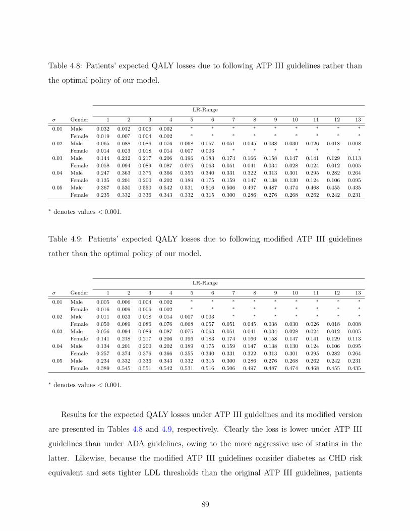
Table 4.8: Patients’ expected QALY losses due to following ATP III guidelines rather than

the optimal policy of our model.

LR-Range

σ Gender 1 2 3 4 5 6 7 8 9 10 11 12 13

0.01 Male 0.032 0.012 0.006 0.002 ∗ ∗ ∗ ∗ ∗ ∗ ∗ ∗ ∗

Female 0.019 0.007 0.004 0.002 ∗ ∗ ∗ ∗ ∗ ∗ ∗ ∗ ∗

0.02 Male 0.065 0.088 0.086 0.076 0.068 0.057 0.051 0.045 0.038 0.030 0.026 0.018 0.008

Female 0.014 0.023 0.018 0.014 0.007 0.003 ∗ ∗ ∗ ∗ ∗ ∗ ∗

0.03 Male 0.144 0.212 0.217 0.206 0.196 0.183 0.174 0.166 0.158 0.147 0.141 0.129 0.113

Female 0.058 0.094 0.089 0.087 0.075 0.063 0.051 0.041 0.034 0.028 0.024 0.012 0.005

0.04 Male 0.247 0.363 0.375 0.366 0.355 0.340 0.331 0.322 0.313 0.301 0.295 0.282 0.264

Female 0.135 0.201 0.200 0.202 0.189 0.175 0.159 0.147 0.138 0.130 0.124 0.106 0.095

0.05 Male 0.367 0.530 0.550 0.542 0.531 0.516 0.506 0.497 0.487 0.474 0.468 0.455 0.435

Female 0.235 0.332 0.336 0.343 0.332 0.315 0.300 0.286 0.276 0.268 0.262 0.242 0.231

∗ denotes values < 0.001.

Table 4.9: Patients’ expected QALY losses due to following modified ATP III guidelines

rather than the optimal policy of our model.

LR-Range

σ Gender 1 2 3 4 5 6 7 8 9 10 11 12 13

0.01 Male 0.005 0.006 0.004 0.002 ∗ ∗ ∗ ∗ ∗ ∗ ∗ ∗ ∗

Female 0.016 0.009 0.006 0.002 ∗ ∗ ∗ ∗ ∗ ∗ ∗ ∗ ∗

0.02 Male 0.011 0.023 0.018 0.014 0.007 0.003 ∗ ∗ ∗ ∗ ∗ ∗ ∗

Female 0.050 0.089 0.086 0.076 0.068 0.057 0.051 0.045 0.038 0.030 0.026 0.018 0.008

0.03 Male 0.056 0.094 0.089 0.087 0.075 0.063 0.051 0.041 0.034 0.028 0.024 0.012 0.005

Female 0.141 0.218 0.217 0.206 0.196 0.183 0.174 0.166 0.158 0.147 0.141 0.129 0.113

0.04 Male 0.134 0.201 0.200 0.202 0.189 0.175 0.159 0.147 0.138 0.130 0.124 0.106 0.095

Female 0.257 0.374 0.376 0.366 0.355 0.340 0.331 0.322 0.313 0.301 0.295 0.282 0.264

0.05 Male 0.234 0.332 0.336 0.343 0.332 0.315 0.300 0.286 0.276 0.268 0.262 0.242 0.231

Female 0.389 0.545 0.551 0.542 0.531 0.516 0.506 0.497 0.487 0.474 0.468 0.455 0.435

∗ denotes values < 0.001.

Results for the expected QALY losses under ATP III guidelines and its modified version

are presented in Tables 4.8 and 4.9, respectively. Clearly the loss is lower under ATP III

guidelines than under ADA guidelines, owing to the more aggressive use of statins in the

latter. Likewise, because the modified ATP III guidelines consider diabetes as CHD risk

equivalent and sets tighter LDL thresholds than the original ATP III guidelines, patients

89

lose more QALYs under the modified version. From Tables 4.7, 4.8 and 4.9, we observe

the QALY loss is more for the male patient; which can be attributed to the earlier onset of

cardiovascular risk.

4.4 CONCLUSIONS

Current lipid management guidelines use long-term CHD risk to make treatment recom-

mendations but do not differentiate patients on the basis of disutility of using statins. In

this chapter we empirically show the importance of tailoring guidelines to short-term CHD

and stroke probabilities, individual patient preferences and patients’ responses to statins.

We gain insights into the effect of medication side effects on treatment decisions and show

that treatment disutility can significantly affect the decision of if and when to initiate statin

treatment. Our numerical results empirically confirm the theoretical results which provide

scientific evidence to help support the practice of threshold-structured treatment policies.

We also illustrate the importance of individualized treatment factors by estimating the pa-

tients’ QALY gains using our customized policies rather than the current U.S. guidelines.

Our experiments indicate that current guidelines may set aggressive thresholds which may

lead up to 0.6 QALY loss per patient.

90

5.0 LIMITATIONS AND FUTURE RESEARCH

This dissertation focuses on two emerging timing problems for diabetes and ESRD patients.

It presents the first stochastic game application in healthcare and the first model in the

literature that aims to balance the trade-off between the benefits and adverse side effects of

statins.

With an ultimate goal of valuing a kidney matching, in Chapter 3 we introduce the

timing of an exchange in a prearranged PKE and formulate the problem resulting between

the patients as a stochastic game. We analyze the underlying equilibria of the game in detail.

In general, showing the existence of a pure equilibrium for stochastic games is challenging.

We use the fact that an exchange does not occur unless both patients offer to exchange

to show that a pure equilibrium always exists for our model. While our model considers

the timing for autonomous and self-interested patients, we recognize the society’s objective

in equilibrium selection. We develop mathematically tractable MIP models to characterize

socially optimal equilibria of the game. We illustrate our analytical results and discuss

their policy implications using clinical data. We observe that randomized strategies perform

negligibly better than pure strategies. We also quantify the social welfare loss due to patient

autonomy and demonstrate that maximizing the number of transplants may be undesirable.

Our numerical study shows that patients may exchange their kidneys prior to the initiation

of dialysis. Therefore, we also shed light on the welfare consequences of preemptive PKEs

which are not common in practice. We believe the model and analyses in this chapter may

also lay the groundwork for exchanges of other organs such as liver and bone marrow, for

which exchanges are not common but matches are difficult to find [48].

The model and analyses in Chapter 3 have some limitations. First, the model does not

consider the arrivals of cadaveric kidneys to any of the patients. In practice because living

91

donors are preferred to cadaveric donors, when patients are both alive they would prefer

the exchange to a cadaveric kidney. In our model, because patient autonomy may delay

the timing of an exchange and one of the patients may die before an exchange occurs, the

surviving patient is assumed to receive no kidneys from the waiting list in the remainder of

her life. However, upon a kidney failure, patients initiate dialysis and register to waiting

list for a cadaveric kidney. We can easily incorporate the effects of possibility of receiving

a cadaveric kidney from the waiting list into the model by modifying the patients’ payoff

functions in (3.1) for s ∈ S and i ∈ N as follows:

gi(s, a1, a2) =

a1(s)a2(s)ui(s, 1) +[1− a1(s)a2(s)

]Fi(s,gi(a1, a2)

)if s ∈ S \D ,

hi(s) otherwise.(5.1)

In (5.1), hi(s) is a one-time termination payoff and represents Patient i’s expected QALYs

when the game terminates in state s due to a death before an exchange occurs and may

include the possibility of receiving a cadaveric kidney from the waiting list after initiating

dialysis. Note that it is a lump-sum reward and equal to 0 if Patient i is dead in state s.

An immediate future research direction would estimate the rewards hi(s) by calibrating

an explicit or implicit waiting list model for ESRD patients and investigate their effects

on patients’ strategies in timing the exchange. In such an extension, because the expected

payoffs in states s ∈ D do not depend on patients’ strategies and rewards hi(s) are

externally estimated, most of our equilibrium conditions would remain valid in all living

states s ∈ S \D and be translated into MIP formulations similar to those of Chapter 3 for

equilibrium selection.

Second, our model treats dialysis initiation as an exogenous probabilistic decision, so

that patients initiate dialysis at practical rates. Dialysis initiation is a complex subject

[114], and requires a more detailed physiological model which may be mathematically in-

tractable and computationally prohibitive within a game-theoretic framework. Third, as

Nash equilibrium eliminates only unilateral deviations, our analyses implicitly assume that

patients can’t collude. Therefore, it ignores the resistance of an equilibrium against patients’

joint deviations. Extension of our analyses to stability-oriented refinements of ordinary Nash

equilibria is a promising future research direction. Last, but not least, our model assumes

92

risk-neutral patients and, our equilibrium analyses and numerical study primarily focus on

welfare-maximizing equilibrium selection. However, patients, especially those with failed

kidneys and severe health progression, may exhibit highly risk-averse behavior in practice

whenever they have a kidney available for transplant. Another promising extension would

incorporate risk-sensitivity into the payoffs and/or consider equilibrium selection for risk-

averse patients, however such an extension would require more sophisticated mathematical

programming representations of the resulting equilibrium conditions.

In Chapter 4 we approach the optimal timing of statin initiation problem by an infinite-

horizon MDP. We derive several structural properties of the resulting optimal policies and

empirically support them using clinical data. We assess the influence of age- and gender-

based risk on the timing of initiation. We also investigate the sensitivity of the resulting

policies with respect to disutility of using statins and the reduction in cholesterol levels by

treatment. We compare the performance of the resulting policies to that of the ATP III

guidelines and show that patients experiencing higher disutility from treatment benefit more

from following the policy suggested by our model than the ATP III guidelines.

The model and the numerical study in Chapter 4 have some limitations. First, the

source data that we use to estimate the progression of LR levels belong to a single medical

center, and the population that the data is drawn from is likely to be healthier than a typical

population that may not receive continuous access to healthcare. Second, a limitation for

our numerical experiments is that we focus only on Caucasian non-smoker patients due to

limited availability of clinical data.

We primarily focus on managing cholesterol levels for Type 2 diabetes and assume that

SBP and HbA1c levels change deterministically as a function of time. In practice statin

treatment may be supported with blood glucose and blood pressure control medications.

An immediate future research would extend the current model in two directions. First, in

addition to LR, it may consider stochastically changing SBP and HbA1c levels. Second,

it may consider the optimization of multiple treatments for each of the aforementioned

risk factors. Note that progressions of LR, SBP and HbA1c are all interrelated as high

blood sugar triggers bad cholesterol and increase in bad cholesterol results in an increase in

blood pressure. Therefore, such a multi-treatment extension would need the joint transition

93

functions of LR, SBP and HbA1c, the estimation of which would be computationally more

sophisticated and need more data for the reliability of the estimates. Moreover, as state

and action spaces will grow exponentially these extensions may suffer from the curse of

dimensionality and necessitate the development of approximation algorithms.

Because a Type 2 diabetes patient’s CHD and stroke risks can be assessed by various

risk models, another future research direction would focus on a robust decision model by

considering the risk model-based ambiguities in the transition probabilities. Such a model

can be further enhanced by incorporating the ambiguities in transitions among LR, SBP and

HbA1c levels that are inherent to estimation under limited data.

94

BIBLIOGRAPHY

[1] A. Abdulkadiroglu and T. Sonmez. House allocation with existing tenants. Journal ofEconomic Theory, 88(2):233–260, 1999.

[2] D. J. Abraham, A. Blum, and T. Sandholm. Clearing algorithms for barter exchangemarkets: Enabling nationwide kidney exchanges. Proceedings of the 8th ACM Confer-ence on Electronic Commerce, 6(4):295–304, 2007.

[3] C. Abramson, I. S. Currim, and R. Sarin. An experimental investigation of the impactof information on competitive decision making. Management Science, 51(2):195–207,2005.

[4] P. D. Ackerman, J. R. Thistlethwaite, and L. F. Ross. Attitudes of minority patientswith end-stage renal disease regarding ABO-incompatible list-paired exchanges. Amer-ican Journal of Transplantation, 6(1):83–88, 2006.

[5] E. Adida, P. C. DeLaurentis, and M. A. Lawley. Hospital stockpiling for disasterplanning. IIE Transactions, 43(5):348–362, 2011.

[6] M. Agraharkar, V. Nair, and M. Patlovany. Recovery of renal function in dialysispatients. BMC Nephrology, 4(9):1–5, 2003.

[7] J. H. Ahn and J. C. Hornberger. Involving patients in the cadaveric kidney transplantallocation process: A decision-theoretic perspective. Management Science, 42(5):629–641, 1996.

[8] O. Alagoz, C. L. Bryce, S. M. Shechter, A. J. Schaefer, C. C. H. Chang, D. C. Angus,and M. S. Roberts. Incorporating biological natural history in simulation models: Em-piric estimates of the progression of end-stage liver disease. Medical Decision Making,25(6):620–632, 2005.

[9] O. Alagoz, H. Hsu, A. J. Schaefer, and M. S. Roberts. Markov decision processes:A tool for sequential decision making under uncertainty. Medical Decision Making,30(4):474–483, 2010.

[10] O. Alagoz, L. M. Maillart, A. J. Schaefer, and M. S. Roberts. The optimal timing ofliving-donor liver transplantation. Management Science, 50(10):1420–1430, 2004.

95

[11] O. Alagoz, L. M. Maillart, A. J. Schaefer, and M. S. Roberts. Choosing among living-donor and cadaveric livers. Management Science, 53(11):1702–1715, 2007.

[12] O. Alagoz, L. M. Maillart, A. J. Schaefer, and M. S. Roberts. Determining the ac-ceptance of cadaveric livers using an implicit model of the waiting list. OperationsResearch, 55(1):24–36, 2007.

[13] Alliance for Paired Donation, 2009. Available from http://www.paireddonation.org.

[14] American Diabetes Association. Standards of medical care in diabetes. Diabetes Care,30(1):S4–S41, 2007.

[15] American Diabetes Association, 2008. Available from http://www.diabetes.org.

[16] American Diabetes Association. Diabetes Fact Sheet, 2012. Available fromhttp://main.diabetes.org/stepup/diabetes facts.pdf. Accessed October 1, 2012.

[17] K. A. Anderson, P. M. Odel, P. W. F. Wilson, and W. B. Kannel. Cardiovasculardisease risk profiles. American Heart Journal, 121(2):293–298, 1991.

[18] A. Arora and M. Ceccagnoli. Patent protection, complementary assets, and firmsincentives for technology licensing. Management Science, 52(2):293–308, 2006.

[19] A. Asderakis, T. Augustine, P. Dyer, C. Short, B. Campbell, N. R. Parrott, andR. W. G. Johnson. Preemptive kidney transplantation: The attractive alternative.Nephrology Dialysis Transplantation, 13(7):1799–1803, 1998.

[20] R. Bala and P. Bhardwaj. Detailing vs. direct-to-consumer advertising in the prescrip-tion pharmaceutical industry. Management Science, 56(1):148–160, 2010.

[21] R. E. Barlow and F. Proschan. Mathematical Theory of Reliability. John Wiley &Sons, New York, NY, 1965.

[22] E. L. Barrett-Connor, B. A. Cohn, D. L. Wingard, and S. L. Edelstein. Why is diabetesmellitus a stronger risk factor for fatal ischemic heart disease in women than in men?Journal of the American Medical Association, 265(5):627–631, 1991.

[23] B. N. Becker, S. H. Rush, D. M. Dykstra, Y. T. Becker, and F. K. Port. Preemptivetransplantation for patients with diabetes-related kidney disease. Archives of InternalMedicine, 166(1):44–48, 2006.

[24] M. L. Brandeau, F. Sainfort, and W. P. Pierskalla. Operations Research and HealthCare: A Handbook of Methods and Applications. Kluwer Academic Publishers, Mas-sachusetts, MA, 2004.

[25] M. Breton. Algorithms for stochastic games. In T. E. S. Raghavan, T. S. Ferguson,T. Parthasarathy, and O. J. Vrieze, editors, Stochastic Games and Related Topics:In Honor of Professor L. S. Shapley, Theory and Decision Library C: Game Theory,

96

Mathematical Programming and Operations Research, pages 45–57. Kluwer AcademicPublishers, 1991.

[26] M. Breton, J. A. Filar, A. Haurie, and T. A. Schultz. On the computation of equi-libria in discounted games. In T. Basar, editor, Dynamic Games and Applications inEconomics, Lecture Notes on Economics and Mathematical Systems. Springer-Verlag,1986.

[27] M. Briel, M. Studer, T. R. Glass, and H. C. Bucher. Effects of statins on strokeprevention in patients with and without coronary heart disease: A meta-analysis ofrandomized controlled trials. American Journal of Medicine, 117(8):596 – 606, 2004.

[28] British Cardiac Society, British Hypertension Society, Diabetes UK, HEART UK, Pri-mary Care Cardiovascular Society and The Stroke Association. JBS 2: Joint BritishSocieties’ guidelines on prevention of cardiovascular disease in clinical practice. Heart,91(S5):1–52, 2005.

[29] V. L. Burt, P. Whelton, E. J. Roccella, C. Brown, J. A. Cutler, M. Higgins, M. J.Horan, and D. Labarthe. Prevalence of hypertension in the U.S. adult population:Results from the 3rd National Health and Nutrition Examination Survey, 1988–1991.Hypertension, 25(3):305–313, 1995.

[30] T. Carrera, L. Bonamusa, L. Almirall, and J. M. Navarro. Should age and sex betaken into account in the determination of HbA1c reference range? Diabetes Care,21(12):2193–2194, 1998.

[31] W. P. Castelli. Epidemiology of coronary heart disease: The Framingham study. TheAmerican Journal of Medicine, 76(2A):4–12, 1984.

[32] Centers for Disease Control. National Chronic Kidney Disease Fact Sheet, 2010. Avail-able from http://www.cdc.gov/diabetes/pubs/pdf/kidney Factsheet.pdf. Accessed Oc-tober 1, 2012.

[33] Centers for Disease Control. National Diabetes Fact Sheet, 2011. Available fromhttp://www.cdc.gov/diabetes/pubs/pdf/ndfs 2011.pdf. Accessed October 1, 2012.

[34] Centers for Medicare and Medicaid Services. NationalHealth Expenditure Projections, 2010. Available fromhttps://www.cms.gov/Research-Statistics-Data-and-Systems/Statistics-Trends-and-Reports/NationalHealthExpendData/downloads/proj2010.pdf. Accessed October1, 2012.

[35] S. E. Chick, H. Mamani, and D. Simchi-Levi. Supply chain coordination and influenzavaccination. Operations Research, 56(6):1493–1506, 2008.

[36] S. H. Cho. The optimal composition of influenza vaccines subject to random productionyields. Manufacturing & Service Operations Management, 12(2):256–277, 2010.

97

[37] H. Colhoun, D. J. Betteridge, P. N. Durrington, G. A. Hitman, H. A. Neil, S. J.Livingstone, M. J. Thomason, M. I. Mackness, V. Charlton-Menys, and J. H. Fuller.Primary prevention of cardiovascular disease with atorvastatin in Type 2 diabetesin the Collaborative Atorvastatin Diabetes Study (CARDS): Multicentre randomisedplacebo-controlled trial. Lancet, 364(9435):685–696, 2004.

[38] A. J. Collins, S. Li, J. Z. Ma, and C. Herzog. Cardiovascular disease in end-stage renaldisease patients. American Journal of Kidney Diseases, 38(4):S26–S29, 2001.

[39] R. Collins, J. Armitage, S. Parish, P. Sleight, and R. Peto. MRC/BHF heart protec-tion study of cholesterol lowering with simvastatin in 20,536 high-risk individuals: Arandomised placebo-controlled trial. Lancet, 360(9426):7–22, 2002.

[40] R. Collins, J. Armitage, S. Parish, P. Sleight, and R. Peto. MRC/BHF heart protec-tion study of cholesterol-lowering with simvastatin in 5963 people with diabetes: Arandomised placebo-controlled trial. Lancet, 361(9374):2005–2016, 2003.

[41] J. Coresh, E. Selvin, L. A. Stevens, J. Manzi, J. W. Kusek, P. Eggers, F. V. Lente,and A. S. Levey. Prevalence of chronic kidney disease in the United States. Journal ofthe American Medical Association, 298(17):2038–2047, 2007.

[42] B. Costa, J. Arroyo, and A. Sabate. The economics of pharmacotherapy for diabetesmellitus. Pharmacoeconomics, 11(2):139–158, 1997.

[43] G. M. Danovitch, D. J. Cohen, M. R. Weir, P. G. Stock, W. M. Bennett, L. L. Chris-tensen, and R. S. Sung. Current status of kidney and pancreas transplantation in theUnited States, 1994-2003. American Journal of Transplantation, 5(2):914–915, 2005.

[44] A. Davenport. Intradialytic complications during hemodialysis. Hemodialysis Interna-tional, 10(2):162–167, 2006.

[45] I. David and U. Yechiali. A time-dependent stopping problem with application to liveorgan transplants. Operations Research, 33(3):491–504, 1985.

[46] I. David and U. Yechiali. Sequential assignment match processes with arrivals of candi-dates and offers. Probability in the Engineering and Informational Sciences, 4(4):413–430, 1990.

[47] I. David and U. Yechiali. One-attribute sequential assignment match processes indiscrete time. Operations Research, 43(5):879–884, 1995.

[48] S. M. Davies, X. O. Shu, B. R. Blazar, A. H. Filipovich, J. H. Kersey, W. Krivit,N. K. C. McCullough, J. Miller, W.J. Ramsay, M. Segall, J. E. Wagner, D. J. Weisdorf,and P. B. McGlave. Unrelated donor bone marrow transplantation: Influence of hlaa and b incompatibility on outcome. RAND Journal of Economics, 86(4):1636–1642,1995.

98

[49] M. de Klerk, K. M. Keizer, F. H. J. Claas, M. Witvliet, B. J. Haase-Kromwijk, andW. Weimar. The Dutch national living-donor kidney exchange program. AmericanJournal of Transplantation, 5(9):2302–2305, 2005.

[50] F. L. Delmonico, R. Arnold, N. Scheper-Hughes, L. A. Siminoff, J. Kahn, and S. J.Youngner. Ethical incentives – not payment – for organ donation. The New EnglandJournal of Medicine, 346(25):2002–2005, 2002.

[51] F. L. Delmonico, P. E. Morrissey, G. S. Lipkowitz, J. S. Stoff, J. Himmelfarb, W. Har-mon, M. Pavlakis, H. Mah, J. Goguen, R. Luskin, E. Milford, G. Basadonna, M. Choba-nian, B. Bouthot, M. Lorber, and R. J. Rohrer. Donor kidney exchanges. AmericanJournal of Transplantation, 4(10):1628–1634, 2004.

[52] B. T. Denton, O. Alagoz, A. Holder, and E. K. Lee. Medical decision making: Openresearch challenges. IIE Transactions on Healthcare Systems Engineering, 1(3):161–167, 2011.

[53] B. T. Denton, M. Kurt, N. D. Shah, S. C. Bryant, and S. A. Smith. Optimizingthe start time of statin therapy for patients with diabetes. Medical Decision Making,29(3):351–368, 2009.

[54] S. Deo and C. J. Corbett. Cournot competition under yield uncertainty: The case ofthe U.S. influenza vaccine market. IIE Transactions, 11(4):563–576, 2009.

[55] S. Deo and I. Gurvich. Centralized vs. decentralized ambulance diversion: A networkperspective. Management Science, 57(7):1300–1319, 2009.

[56] R. Dinavahi and E. Akalin. Preemptive kidney transplantation in patients with diabetesmellitus. Endocrinology and Metabolism Clinics of North America, 36(4):1039–1049,2007.

[57] P. Donnelly, P. Oman, R. Henderson, and G. Opelz. Living-donor kidney transplanta-tion in predialysis patients: Experience of marginal donors in Europe and the UnitedStates. Transplantation Proceedings, 28(6):3566–3570, 1996.

[58] J. R. Downs, M. Clearfield, S. Weis, E. Whitney, D. R. Shapiro, P.A. Beere, and AirForce/Texas Coronary Atherosclerosis Prevention Study Group. Primary preventionof acute coronary events with lovastatin in men and women with average cholesterollevels: Results of AFCAPS/TexCAPS. Journal of the American Medical Association,279(20):1615–1622, 1998.

[59] M. F. Drummond, B. O’Brien, G. L. Stoddart, and G. W. Torrance. Methods for theEconomic Evaluation of Health Care Programmes. Oxford University Press, Oxford,England, 2005.

[60] D. M. Eddy and L. Schlessinger. Archimedes - a trial-validated model of diabetes.Diabetes Care, 26(11):3093–3101, 2003.

99

[61] D. M. Eddy and L. Schlessinger. Validation of the Archimedes diabetes model. DiabetesCare, 26(11):3102–3110, 2003.

[62] J. Edmonds. Paths, trees, and flowers. Canadian Journal of Mathematics, 17:449–467,1965.

[63] J. A. Filar and T. A. Schultz. Nonlinear programming and stationary strategies instochastic games. Mathematical Programming, 34(2):243–247, 1986.

[64] J. A. Filar, T. A. Schultz, F. Thuijsman, and O. J. Vrieze. Nonlinear programming andstationary equilibria in stochastic games. Mathematical Programming, 50(2):227–237,1991.

[65] J. A. Filar and K. Vrieze. Competitive Markov Decision Processes. Springer, NewYork, NY, 1996.

[66] A. M. Fink. Equilibrium in a stochastic N -person game. Journal of Science of theHiroshima University, 28(1):89–93, 1964.

[67] Fourth Joint Task Force of the European Society of Cardiology. European guidelineson cardiovascular disease prevention in clinical practice: Executive summary. EuropeanHeart Journal, 194(1):1–45, 2007.

[68] B. E. Fries. Bibliography of operations research in health-care systems. OperationsResearch, 24(5):801–814, 1976.

[69] D. Fudenberg and J. Tirole. Game Theory. MIT Press, Cambridge, MA, 1990.

[70] P. C. Fuloria and S. A. Zenios. Outcomes-adjusted reimbursement in a health-caredelivery system. Management Science, 47(6):735–751, 2001.

[71] D. Gale and L. S. Shapley. College admissions and the stability of marriage. TheAmerican Mathematical Monthly, 69(1):9–15, 1962.

[72] A. Ganesh and K. Lee. Management of chronic kidney disease and end-stage renaldisease in diabetes. The University of British Columbia Medical Journal, 3(1):13–16,2011.

[73] J. J. Ganuza, G. Llobet, and B. Domnguez. R&D in the pharmaceutical industry: Aworld of small innovations. Management Science, 55(4):539–551, 2009.

[74] S. Ganzfried and T. Sandholm. Computing equilibria in multiplayer stochastic gamesof imperfect information. In Proceedings of the 21st International Joint Conference onArtifical Intelligence, IJCAI’09, pages 140–146, 2009.

[75] A.R. Garber, R.A. Olshen, H. Zhang, and E.S. Venatraman. Predicting high riskcholesterol levels. International Statistical Review, 62(2):203–228, 1994.

100

[76] S. E. Gentry, D. L. Segev, and R. A. Montgomery. A comparison of populations servedby kidney paired donation and list-paired donation. American Journal of Transplan-tation, 5(8):1914–1921, 2005.

[77] S. E. Gentry, D. L. Segev, M. Simmerling, and R. A. Montgomery. Expanding kid-ney paired donation through participation by compatible pairs. American Journal ofTransplantation, 7(10):2361–2370, 2007.

[78] J. Gilbert, L. Brigham, D. S. Batty, and R. M. Veatch. The nondirected living-donorprogram: A model for cooperative donation, recovery and allocation of living-donorkidneys. American Journal of Transplantation, 5(1):167–174, 2005.

[79] J. S. Gill, M. Tonelli, N. Johnson, and B. J. G. Pereira. Why do preemptive kidneytransplant recipients have an allograft survival advantage? Transplantation, 78(6):873–887, 2004.

[80] D. W. Gjertson and J. M. Cecka. Living unrelated donor kidney transplantation.Kidney International, 58(2):491–499, 2000.

[81] A. S. Go, G. M. Chertow, D. Fan, C. E. McCulloch, and C. Hsu. Chronic kidneydisease and the risks of death, cardiovascular events, and hospitalization. The NewEngland Journal of Medicine, 351(13):1296–1305, 2004.

[82] M. R. Gold, D. L. Patrick, G. W. Torrance, D. G. Fryback, D. C. Hadorn, M. S.Kamlet, N. Daniels, and M. C. Weinstein. Identifying and valuing outcomes. In M. R.Gold, J. E. Siegel, L. B. Russell, and M. C. Weinstein, editors, Cost-Effectiveness inHealth and Medicine, pages 82–134. Oxford University Press, 1996.

[83] M. R. Gold, D. Stevenson, and D.G. Fryback. HALYs and QALYs and DALYs, ohmy: Similarities and differences in summary measures of population health. AnnualReview of Public Health, 23:115–134, 2002.

[84] C. A. Gorman, B. R. Zimmerman, S. A. Smith, S. F. Dinneen, J. B. Knudsen, D. Holm,B. Jorgensen, S. Bjornsen, K. Planet, P. Hanson, and R. A. Rizza. DEMS - a secondgeneration diabetes electronic management system. Computer Methods and Programsin Biomedicine, 62(2):127–140, 2000.

[85] M. Gray. Value: Operations research and the new health care paradigm. OperationsResearch for Health Care, 1(1):20–21, 2012.

[86] J. L. Gross, M. J. De Azevedo, S. P. Silveiro, L. H. Canani, M. L. Caramori, andT. Zelmanovitz. Diabetic nephropathy: Diagnosis, prevention, and treatment. DiabetesCare, 28(1):164–176, 2005.

[87] I. Hajjar and T. A. Kotchen. Trends in prevalence, awareness, treatment, and controlof hypertension in the United States, 1988–2000. Journal of the American MedicalAssociation, 290(2):199–206, 2003.

101

[88] P. R. Hebert, J. M. Gaziano, K. S. Chan, and C. H. Hennekens. Cholesterol loweringwith statin drugs, risk of stroke, and total mortality - an overview of randomized trials.Journal of the American Medical Association, 278(4):313–321, 1997.

[89] P. J. J. Herings and R. J. A. P. Peeters. Equilibrium selection in stochastic games.International Game Theory Review, 5(1):307–326, 2003.

[90] P. J. J. Herings and R. J. A. P. Peeters. Stationary equilibria in stochastic games:Structure, selection, and computation. Journal of Economic Theory, 118(1):32–60,2004.

[91] A. A. Honeycutt, J. P. Boyle, K. R. Broglio, T. J. Thompson, T. J. Hoerger, L. S.Geiss, and K. M. Venkat Narayan. A dynamic Markov model for forecasting dia-betes prevalence in the United States through 2050. Health Care Management Science,6(3):155–164, 2003.

[92] J. C. Hornberger and J. H. Ahn. Deciding eligibility for transplantation when a donorkidney becomes available. Medical Decision Making, 17(2):160–170, 1997.

[93] D. H. Howard. Why do transplant surgeons turn down organs? A model of theaccept/reject decision. Journal of Health Economics, 21(6):957–969, 2002.

[94] Q. Hu, L. B. Schwarz, and N. A. Uhan. The impact of group purchasing organizationson healthcare-product supply chains. Manufacturing & Service Operations Manage-ment, 14(1):9–23, 2012.

[95] L. Hurwicz. Optimality and informational efficiency in resource allocation processes.In K. J. Arrow, S. Karlin, and P. Suppes, editors, Mathematical Methods in the SocialSciences, pages 27–46. Stanford University Press, 1960.

[96] M. Jackson. Mechanism theory. In U. Derigs, editor, The Encyclopedia of Life SupportSystems. EOLSS Publishers, 2003.

[97] A. G. John, M. Rao, and C. K. Jacob. Preemptive live-related renal transplantation.Transplantation, 66(2):204–209, 1998.

[98] D. Kahaner, C. Moler, and S. Nash. Numerical Methods and Software. Prentice Hall,Upper Saddle River, NJ, 1989.

[99] W. B. Kannel. Blood pressure as a cardiovascular risk factor. Journal of the AmericanMedical Association, 275(20):1571 – 1576, 1996.

[100] I. Kaplan, J. A. Houp, M. S. Leffell, J. M. Hart, and A. A. Zachary. A computermatch program for paired and unconventional kidney exchanges. American Journal ofTransplantation, 5(9):2306–2308, 2005.

[101] I. Karp, S. F. Chen, and L. Pilote. Sex differences in the effectiveness of statins aftermyocardial infarction. Canadian Medical Association Journal, 176(3):333–338, 2007.

102

[102] B. L. Kasiske, D. Cohen, M. R. Lucey, and J. F. Neylan. Payment for immunosuppres-sion after organ transplantation. The Journal of the American Medical Association,283(18):2445–2450, 2000.

[103] K. M. Keizer, M. de Klerk, B. J. Haase-Kromwijk, and W. Weimar. The Dutchalgorithm for allocation in living-donor kidney exchange. Transplantation Proceedings,37(2):589–591, 2005.

[104] Kidney and Urology Foundation of America. Kid-ney Disease of Diabetes, 2012. Available fromhttp://www.kidneyurology.org/Library/Kidney Health/Kidney Disease of Diabetes.php.Accessed October 1, 2012.

[105] E. S. Kilpatrick, M. H. Dominiczak, and M. Small. The effects of ageing on glycationand the interpretation of glycaemic control in Type 2 diabetes. The Quarterly Journalof Medicine: An International Journal of Medicine, 89(4):307–312, 1996.

[106] P. Koskinen, M. Manttari, V. Manninen, J. K. Huttunen, O. P. Heinonen, and M. H.Frick. Coronary heart disease incidence in NIDDM patients in the Helsinki HeartStudy. Diabetes Care, 15(7):820–825, 1992.

[107] V. Kothari, R. J. Stevens, A. I. Adler, I. M. Stratton, S. E. Manley, H.A. Neil, andR. R. Holman. UKPDS 60 - risk of stroke in Type 2 diabetes estimated by the UKProspective Diabetes Study risk engine. Stroke, 33(7):1776–1781, 2002.

[108] R. M. Krauss. Lipids and lipoproteins in patients with type 2 diabetes. Diabetes Care,27(6):1496–1504, 2004.

[109] J. E. Kreke, M. D. Bailey, A. J. Schaefer, M. S. Roberts, and D. C. Angus. Modelinghospital discharge policies for patients with pneumonia-related sepsis. IIE Transac-tions, 40(9):861–869, 2008.

[110] V. Kulkarni. Stochastic Models in Health Care, 2012. Available fromhttp://www.unc.edu/~vkulkarn/STOR892-2012/notes.pdf. Accessed October 27,2012.

[111] M. Kurt, B. T. Denton, A. J. Schaefer, N. D. Shah, and S. A. Smith. The structureof optimal statin initiation policies for patients with type 2 diabetes. IIE Transactionson Healthcare Systems Engineering, 1(1):49–65, 2011.

[112] A. Laupacis, P. Keown, N. Pus, H. Krueger, B. Ferguson, C. Wong, and N. Muir-head. A study of the quality of life and cost-utility of renal transplantation. KidneyInternational, 50(1):235–242, 1996.

[113] C. B. Lee, W. D. Murphy, L. R. Fletcher, and J. M. Binner. Dynamic entry deter-rence in the UK pathology services market. European Journal of Operational Research,105(2):296–307, 1998.

103

[114] C. P. Lee, G. M. Chertow, and S. A. Zenios. Optimal initiation and management ofdialysis therapy. Operations Research, 56(6):1428–1449, 2008.

[115] H. Lee, B. Manns, K. Taub, W. A. Ghali, S. Dean, D. Johnson, and C. Donaldson.Cost analysis of ongoing care of patients with end-stage renal disease: The impact ofdialysis modality and dialysis access. American Journal of Kidney Diseases, 40(3):611–622, 2002.

[116] G. Lim and E. K. Lee. Optimization in Medicine and Biology. Auerbach Publications,Boca Raton, FL, 2008.

[117] J. A. Macdonald, S. P. McDonald, C. M. Hawley, J. Rosman, F. Brown, K. J. Wig-gins1, K. Bannister, and D. W. Johnson. Recovery of renal function in end-stage renalfailure-comparison between peritoneal dialysis and hemodialysis. Nephrology DialysisTransplantation, 24(9):2825–2831, 2009.

[118] A. O. Mahendran and P. S. Veitch. Paired exchange programmes can expand the livekidney donor pool. British Journal of Surgery, 94(6):657–664, 2007.

[119] K. C. Mange, M. M. Joffe, and H. I. Feldman. Effect of the use or nonuse of long-termdialysis on the subsequent survival of renal transplants from living-donors. The NewEngland Journal of Medicine, 344(10):726–731, 2001.

[120] K. C. Mange and M. R. Weir. Preemptive renal transplantation: Why not? AmericanJournal of Transplantation, 3(11):1336–1340, 2003.

[121] J. A. E. Manson, G. A. Colditz, M. J. Stampfer, W. C. Willett, A. S. Krolewski,B. Rosner, R. A. Arky, F. E. Speizer, and C. H. A. Hennekens. A prospective studyof maturity-onset diabetes mellitus and risk of coronary heart disease and stroke inwomen. Annals of Internal Medicine, 151(6):1141–1147, 1991.

[122] D. J. Maron, S. Fazio, and M. F. Linton. Current perspectives on statins. Circulation,101(2):207–213, 2000.

[123] A. Mas-Colell, M. D. Whinston, and J. R. Green. Microeconomic Theory. OxfordUniversity Press, New York, NY, 1995.

[124] E. Maskin and J. Tirole. Markov perfect equilibrium: I. Observable actions. Journalof Economic Theory, 100(2):191–219, 2001.

[125] J. Mason and B. T. Denton. A comparison of decision maker perspectives for optimalcholesterol treatment. To appear in IBM Journal on Research and Development.

[126] J. E. Mason, D. England, B. T. Denton, S. A. Smith, M. Kurt, and N. D. Shah.Optimizing statin treatment decisions in the presence of uncertain future adherence.Medical Decision Making, 32(1):154–166, 2012.

104

[127] D. B. McLaughlin and J. M. Hays. Healthcare Operations Management. Health Ad-ministration Press, Chicago, IL, 2008.

[128] R. Mehrotra, Y. W. Chiu, K. K. Zadeh, J. Bargman, and E. Vonesh. Similar outcomeswith hemodialysis and peritoneal dialysis in patients with end-stage renal disease.Archives of Internal Medicine, 171(2):162–167, 2011.

[129] H. U. Meier-Kriesche and B. Kaplan. Waiting time on dialysis as the strongest modifi-able risk factor for renal transplant outcomes: A paired donor kidney analysis. Trans-plantation, 74(23):1377–1381, 2002.

[130] H. U. Meier-Kriesche, F. K. Port, A. O. Ojo, S. M. Rudich, J. A. Hanson, D. M. Cibrik,A. B. Leichtman, and B. Kaplan. Effect of waiting time on renal transplant outcome.Kidney International, 58(3):1311–1317, 2000.

[131] R. A. Montgomery, C. E. Simpkins, and D. L. Segev. New options for patients withdonor incompatibilities. Transplantation, 82(2):164–165, 2006.

[132] R. A. Montgomery, A. A. Zachary, L. E. Ratner, D. L. Segev, J. M. Hiller, J. Houp,M. Cooper, L. Kavoussi, T. Jarrett, J. Burdick, W. R. Maley, J. K. Melancon, T. Ko-zlowski, C. E. Simpkins, M. Phillips, A. Desai, B. Reeb, E. Kraus, H. Rabb, M. S.Leffell, and D. S. Warren. Clinical results from transplanting incompatible live kid-ney donor/recipient pairs using kidney paired donation. The Journal of the AmericanMedical Association, 294(13):1655–1663, 2005.

[133] P. E. Morrissey. In support of list-paired exchange. American Journal of Transplanta-tion, 6(2):434–435, 2006.

[134] National Center for Health Statistics (NCHS). Mortality data from the National VitalStatistics System, 2005. Available from http://www.cdc.gov/nchs/deaths.htm. Ac-cessed November 1, 2009.

[135] National Cholesterol Education Program. Executive summary of the 2nd report of theNCEP expert panel on detection, evaluation, and treatment of high blood cholesterolin adults (Adult Treatment Panel II). Circulation, 89(3):1329–1445, 1994.

[136] National Cholesterol Education Program. Executive summary of the 3rd report of theNCEP expert panel on detection, evaluation, and treatment of high blood cholesterolin adults (Adult Treatment Panel III). Journal of the American Medical Association,285(19):2486–2497, 2001.

[137] National Heart Foundation of Australia, and The Cardiac Society of Australia and NewZealand. Lipid management guidelines supplement. The Medical Journal of Australia,175:s57–s88, 2001.

105

[138] National Kidney and Urologic Diseases Information Clearinghouse. Kidney Diseaseof Diabetes, 2012. Available from http://kidney.niddk.nih.gov/kudiseases/pubs/kdd/.Accessed October 1, 2012.

[139] National Kidney Foundation, 2010. Available from http://www.kidney.org.

[140] New England Program for Kidney Exchange, 2009. Available fromhttp://www.nepke.org.

[141] New Zealand Guidelines Group. The assessment and management of cardiovascularrisk, 2003. Available from http://www.nzgg.org.nz. Accessed May 1, 2009.

[142] A. Neyman and S. Sorin. Stochastic Games and Applications. Kluwer Academic Pub-lishers, Dordrecht, The Netherlands, 2003.

[143] Y. C. Ng, P. Jacobs, and J. A. Johnson. Productivity losses associated with diabetesin the U.S. Diabetes Care, 24(2):257–261, 2001.

[144] G. Opelz. HLA compatibility and kidney grafts from unrelated live donors. Transplan-tation Proceedings, 30(3):704–705, 1998.

[145] Y. A. Ozcan. Quantitative Methods in Health Care Management: Techniques andApplications. Jossey-Bass, San Francisco, CA, 2005.

[146] A. Pakes and P. McGuire. Stochastic algorithms, symmetric Markov perfect equilib-rium, and the curse of dimensionality. Econometrica, 69(5):1261–1281, 2001.

[147] P. M. Pardalos and H. E. Romeijn. Handbook of Optimization in Medicine. Springer-Verlag, New York, NY, 2008.

[148] K. Park, J. H. Lee, K. H. Huh, S. I. Kim, and Y. S. Kim. Exchange living-donor kidneytransplantation: Diminution of donor organ shortage. Transplantation Proceedings,36(10):2949–2951, 2004.

[149] K. Park, J. I. Moon, S. I. Kim, and Y. S. Kim. Exchange donor program in kidneytransplantation. Transplantation, 67(1):336–338, 1999.

[150] S. Pastan and J. Bailey. Dialysis therapy. The New England Journal of Medicine,338(20):1428–1437, 1998.

[151] R. C. Pasternak, S. C. Smith, Jr. C. N. Bairey-Merz, S. M. Grundy, J. I. Cleeman,and C. Lenfant. ACC/AHA/NHLBI clinical advisory on the use and safety of statins.Journal of the American College of Cardiology, 40(3):567–572, 2002.

[152] T. Phan, J. G. MeLeod, J. D. Pollard, O. Peiris, A. Rohan, and J. P. Halpern. Pe-ripheral neuropathy associated with simvastatin. Journal of the American MedicalAssociation, 58(1):625–628, 1995.

106

[153] P. S. Phillips, R. H. Haas, S. Bannykh, N. L. Hathaway, S. Gray, and B. J. Kimura.Statin-associated myopathy with normal creatine kinase levels. Annals of InternalMedicine, 137(7):581–585, 2002.

[154] W. P. Pierskalla and D. J. Brailer. Applications of Operations Research in HealthcareDelivery. In: Handbooks in Operations Research and Management Science, 6: Op-erations Research and the Public Sector, S. M. Pollock, M. H. Rothkopf, A. Barnett(Eds.), Elsevier, Amsterdam, The Netherlands, 1994.

[155] M. Pignone, S. Earnshaw, J. A. Tice, and M. J. Pletcher. Aspirin, statins, or bothdrugs for the primary prevention of coronary heart disease events in men: A cost-utilityanalysis. Annals of Internal Medicine, 144(5):326–336, 2006.

[156] L. Pilote, K. Dasgupta, V. Guru, K. H. Humphries, J. McGrath, C. Norris, D. Rabi,J. Tremblay, A. Alamian, T. Barnett, J. Cox, W. A. Ghali, S. Grace, P. Hamet, T. Ho,S. Kirkland, M. Lambert, D. Libersan, J. O’Loughlin, G. Paradis, M. Petrovich, andV. Tagalakis. A comprehensive view of sex-specific issues related to cardiovasculardisease. Canadian Medical Association Journal, 176(6):S1–44, 2007.

[157] Organ Procurement and Transplantation Network. 2009 OPTN / SRTRAnnual Report: Transplant Data 1999-2008, 2011. Available fromhttp://optn.transplant.hrsa.gov/ar2009. Accessed June 15, 2011.

[158] Organ Procurement and Transplantation Network. Kidney paired do-nation pilot program operational guidelines, 2011. Available fromhttp://optn.transplant.hrsa.gov/resources/KPDPP.asp. Accessed June 15, 2011.

[159] Organ Procurement and Transplantation Network. National KPD pilot program pro-posal, 2011. Available from http://optn.transplant.hrsa.gov/resources/KPDPP.asp.Accessed June 15, 2011.

[160] Organ Procurement and Transplantation Network. Organ distri-bution: Allocation of deceased kidneys, 2011. Available fromhttp://optn.transplant.hrsa.gov/PoliciesandBylaws2/policies/pdfs. Accessed June15, 2011.

[161] M. L. Puterman. Markov Decision Processes: Discrete Stochastic Dynamic Program-ming. John Wiley & Sons, New York, NY, 1994.

[162] A. Rais and A. Viana. Operations research in healthcare: A survey. InternationalTransactions in Operational research, 18(1):1–31, 2011.

[163] S. Ramsey, K. H. Summers, S. A. Leong, H. G. Birnbaum, J. E. Kemner, and P. Green-berg. Productivity and medical costs of diabetes in a large employer population. Dia-betes Care, 25(1):23–29, 2002.

107

[164] F. T. Rapaport. The case for a living emotionally related international kidney donorexchange registry. Transplantation Proceedings, 18(3):5–9, 1986.

[165] E. Rasmusen. Games and Information: An introduction to Game Theory. Wiley-Blackwell, Malden, MA, 2001.

[166] U. Rieder. Equilibrium plans for non-zero sum markov games. In O. Moeshlin andD. Pallaschke, editors, Game Theory and Related Topics, pages 91–101. North-HollandPublishing Company, 1979.

[167] R. Righter. A resource allocation problem in a random environment. OperationsResearch, 37(2):329–338, 1989.

[168] L. F. Ross and E. S. Woodle. Ethical issues in increasing living kidney donations byexpanding kidney paired exchange programs. Transplantation, 69(8):1539–1543, 2000.

[169] L. F. Ross and S. A. Zenios. Restricting living-donor-cadaver-donor exchanges toensure that standard blood type O wait-list candidates benefit. American Journal ofTransplantation, 78(5):641–646, 2004.

[170] A. E. Roth, T. Sonmez, and M. U. Unver. Kidney exchange. Quarterly Journal ofEconomics, 119(2):457–488, 2004.

[171] A. E. Roth, T. Sonmez, and M. U. Unver. A kidney exchange clearinghouse in NewEngland. American Economic Review, 95(2):376–380, 2005.

[172] A. E. Roth, T. Sonmez, and M. U. Unver. Pairwise kidney exchange. Journal ofEconomic Theory, 125(2):151–188, 2005.

[173] A. E. Roth, T. Sonmez, and M. U. Unver. Efficient kidney exchange: Coincidence ofwants in markets with compatibility-based preferences. American Economic Review,97(3):828–851, 2007.

[174] A. E. Roth, T. Sonmez, M. U. Unver, L. F. Delmonico, and S. L. Saidman. Utilizinglist exchange and undirected good Samaritan donation through ‘chain’ paired kidneyexchanges. American Journal of Transplantation, 6(11):2694–2705, 2006.

[175] S. L. Saidman, A. E. Roth, T. Sonmez, M. U. Unver, and F. L. Delmonico. Increasingthe opportunity of live kidney donation by matching for two and three way exchanges.Transplantation, 81(5):773–782, 2006.

[176] B. Sandıkcı. Estimating the price of privacy in liver transplantation, 2008. Ph.DDissertation, University of Pittsburgh.

[177] B. Sandıkcı, L. M. Maillart, A. J. Schaefer, O. Alagoz, and M. S. Roberts. Estimatingthe patient’s price of privacy in liver transplantation. Operations Research, 56(6):1393–1410, 2008.

108

[178] M. A. Schnitzler, J. F. Whiting, D. C. Brennan, G. Lin, W. Chapman, J. Lowell,S. Boxerman, K. L. Hardinger, and Z. Kalo. The expanded criteria donor dilemma incadaveric renal transplantations. Transplantation, 75(12):1940–1945, 2003.

[179] J. Schwartz, M. D. Stegall, W. K. Kremers, and J. Gloor. Complications, resourceutilization, and cost of ABO incompatible living-donor kidney transplantation. Trans-plantation, 82(2):155–163, 2000.

[180] Scientific Registry of Transplant Recipients. Extrapolation methods: Approximatingthe median survival time beyond the duration of follow-up based on geometric andlinear growth in death rates, 2007. Working paper.

[181] Scientific Registry of Transplant Recipients, 2009. Available fromhttp://www.ustransplant.org.

[182] D. L. Segev, S. E. Gentry, J. K. Melancon, and R. A. Montgomery. Characterizationof waiting times in a simulation of kidney paired donation. American Journal ofTransplantation, 5(10):2448 – 2455, 2005.

[183] D. L. Segev, S. E. Gentry, and R. A. Montgomery. Association between waiting timesfor kidney transplantation and rates of live donation. American Journal of Transplan-tation, 7(10):2406–2413, 2007.

[184] D. L. Segev, L. M. Kucirka, S. E. Gentry, and R. A. Montgomery. Utilization andoutcomes of kidney paired donation in the United States. Transplantation, 86(4):502–510, 2008.

[185] R. A. Sells, L. F. Ross, E. S. Woodle, and M. Siegler. Paired kidney exchange programs.The New England Journal of Medicine, 337(19):1392–1393, 2005.

[186] N. D. Shah, B. T. Denton, M. Kurt, A. J. Schaefer, S. A. Smith, and V. M. Montori.Comparative effectiveness of guidelines for the management of hyperlipidemia andhypertension for type 2 diabetes patients. PLoS ONE, 6(1):e16170, 2011.

[187] L. Shapley and H. Scarf. On cores and indivisibilities. Journal of Mathematical Eco-nomics, 1(1):23–27, 1974.

[188] L. S. Shapley. Stochastic games. Proceedings of the National Academy of Sciences,39(10):1095–1100, 1953.

[189] S. Shechter. Optimal scheduling of highly active antiretroviral therapies for H.I.V.patients, 2006. Ph.D Dissertation, University of Pittsburgh.

[190] L. J. Shuman, R. D. Speas, and J. P. Young. Operations Research in Health Care. TheJohns Hopkins University Press, Baltimore, MD, 1975.

[191] J. M. Smith. Evolution and the Theory of Games. Cambridge University Press, NewYork, NY, 1982.

109

[192] V. Snow, M. D. Aronson, E. R. Hornbake, C. Mottur-Pilson, and K. B Weiss. Lipidcontrol in the management of Type 2 diabetes mellitus: A clinical practice guidelinefrom the American College of Physicians. Annals of Internal Medicine, 140(8):644–649,2004.

[193] M. J. Sobel. Noncooperative stochastic games. Annals of Mathematical Statistics,42(6):1930–1935, 1971.

[194] Y. K. Son, J. S. Oh, S. M. Kim, J. M. Jeon, Y. H. Shin, and J. K. Kim. Clini-cal outcome of preemptive kidney transplantation in patients with diabetes mellitus.Transplantation Proceedings, 42(9):3497–3502, 2010.

[195] T. Sonmez and M. U. Unver. House allocation with existing tenants: A characteriza-tion. Games and Economic Behavior, 69(2):425–445, 2010.

[196] J. Stamler, O. Vaccaro, J. D. Neaton, and D. Wentworth. Diabetes, other risk factors,and 12-year cardiovascular mortality for men screened in the Multiple Risk FactorIntervention Trial. Diabetes Care, 16(2):434–444, 1993.

[197] M. D. Stegall, P. G. Dean, and Gloor J. M. ABO-incompatible kidney transplantation.Transplantation, 78(5):635–640, 2004.

[198] R. J. Stevens, V. Kothari, A. I. Adler, I. M. Stratton, and R. R. Holman. The UKPDSrisk engine: A model for the risk of coronary heart disease in Type 2 diabetes (UKPDS56). Clinical Science, 101(6):671–679, 2001.

[199] X. Su and S. A. Zenios. Patient choice in kidney allocation: The role of the queueingdiscipline. Manufacturing & Service Operations Management, 6(4):280–301, 2004.

[200] X. Su and S. A. Zenios. Patient choice in kidney allocation: A sequential stochasticassignment model. Operations Research, 53(3):443–455, 2005.

[201] X. Su and S. A. Zenios. Recipient choice can address the efficiency-equity trade-off in kidney transplantation: A mechanism design model. Management Science,52(11):1647–1660, 2006.

[202] P. Sun, L. Yang, and F. de Vericourt. Selfish drug allocation for containing an in-ternational influenza pandemic at the onset. Operations Research, 57(6):1320–1332,2009.

[203] L. A. Szczech and I. L. Lazar. Projecting the United States ESRD population: Issuesregarding treatment of patients with ESRD. Kidney International, 66(S90):S3–S7,2004.

[204] M. Takahashi. Equilibrium points of stochastic, noncooperative N -person games. Jour-nal of Science of the Hiroshima University, 28(1):95–99, 1964.

110

[205] P. I. Terasaki, J. M. Cecka, D. W. Gjertson, and S. Takemoto. High survival ratesof kidney transplants from spousal and living unrelated donors. The New EnglandJournal of Medicine, 333(6):333–336, 1995.

[206] M. A. Testa and D. C. Simonson. Health economic benefits and quality of life during im-proved glycemic control in patients with Type 2 diabetes mellitus - a randomized, con-trolled, double-blind trial. Journal of the American Medical Association, 280(17):1490–1496, 1998.

[207] The National Kidney Foundation. Diabetes and Chronic Kidney Disease, 2007. Avail-able from http://www.kidney.org/atoz/pdf/diabetes.pdf. Accessed October 1, 2012.

[208] The National Kidney Foundation. Organ Donation and Transplantation, 2012. Avail-able from http://www.kidney.org/transplantation/livingdonors/infoqa.cfm. AccessedOctober 1, 2012.

[209] The United States Renal Data System. Costs of ESRD, 2011. Available fromhttp://www.usrds.org/2011/pdf/v2 ch011 11.pdf. Accessed October 1, 2012.

[210] The USRDS Annual Report, 2009. Available from http://www.usrds.org/adr.htm.

[211] P. D. Thompson, P. Clarkson, and R. H. Karas. Statin-associated myopathy. Journalof the American Medical Association, 289(1):1681–1690, 2003.

[212] J. Tsevat, K. M. Kuntz, E. J. Orav, M. C. Weinstein, F. M. Sacks, and L. Goldman.Cost-effectiveness of pravastatin therapy for survivors of myocardial infarction withaverage cholesterol levels. American Heart Journal, 141(5):727–734, 2001.

[213] R. C. Turner. The UK Prospective Diabetes Study - A review. Diabetes Care, 21:C35–C38, 1998.

[214] UKPDS Group. Intensive blood glucose control with sulphonylureas or insulin com-pared with conventional treatment and risk of complications in patients with Type 2diabetes (UKPDS 33). Lancet, 352(6):837–853, 1998.

[215] United Network for Organ Sharing. Available from http://www.unos.org.

[216] UNOS - The Organ Procurement and Transplantation Network (OPTN) NationalData, 2009. http://www.optn.org/data. Accessed May 1, 2010.

[217] M. U. Unver. Dynamic kidney exchange. Review of Economic Studies, 77(1):372–414,2010.

[218] J. Valabhji. Dyslipidemia in Type 2 diabetes: epidemiology and biochemistry. TheBritish Journal of Diabetes and Vascular Disease, 3(3):184–189, 2003.

111

[219] C. Valdez-Flores and R. M. Feldman. A survey of preventive maintenance models forstochasically deteriorating single-unit systems. Naval Research Logistics, 36(4):419 –446, 1989.

[220] R. M. Veatch. Organ exchanges: Fairness to the O-blood group. American Journal ofTransplantation, 6(1):1–2, 2006.

[221] N. Vieille. Stochastic games: Recent results. In R. J. Aumann and S. Hart, editors,Handbook of Game Theory with Economic Applications, volume 3, pages 1833–1850.Elsevier, 2002.

[222] S. Vijan and R. A. Hayward. Pharmacologic lipid-lowering therapy in Type 2 diabetesmellitus: Background paper for the American College of Physicians. Annals of InternalMedicine, 140(8):650–658, 2004.

[223] J. M. E. Walsh and M. Pignone. Drug treatment of hyperlipidemia in women. Journalof the American Medical Association, 291(18):2243–2252, 2004.

[224] A. Y. M. Wang. Cardiovascular risk in diabetic end-stage renal disease patients. Journalof Diabetes, 3(2):119–131, 2011.

[225] S. Wang, F. de Vericourt, and P. Sun. Decentralized resource allocation to control anepidemic: A game theoretic approach. Mathematical Biosciences, 222(1):1–12, 2009.

[226] S. G. Wannamethee, A. G. Shaper, and S. Ebrahim. HDL-cholesterol, total cholesterol,and the risk of stroke in middle-aged British men. Stroke, 31(8):1882–1888, 2000.

[227] G. R. Warnick, R. H. Knopp, V. Fitzpatrick, and L. Branson. Estimating low-densitylipoprotein cholesterol by the Friedewald equation is adequate for classifying patientson the basis of nationally recommended cutpoints. Clinical Chemistry, 36(1):15 – 19,1990.

[228] W. C. Winkelmayer, M. C. Weinstein, M. A. Mittleman, R. J. Glynn, and J. S. Pliskin.Health economic evaluations: The special case of end-stage renal disease treatment.Medical Decision Making, 22(5):417–430, 2002.

[229] R. A. Wolfe, V. B. Ashby, E. L. Milford, A. O. Ojo, R. E. Ettenger, L. Y. Agodoa,P. J. Held, and F. K. Port. Comparison of mortality in all patients on dialysis, patientson dialysis awaiting transplantation, and recipients of a first cadaveric transplant. TheNew England Journal of Medicine, 341(23):1725–1730, 1999.

[230] R. A. Wolfe, K. P. McCullough, D. E. Schaubel, J. D. Kalbfleisch, S. Murray, M. D.Stegall, and A. B. Leichtman. Calculating life years from transplant (LYFT): Methodsfor kidney and kidney-pancreas candidates. American Journal of Transplantation,8(2):997–1011, 2008.

[231] E. S. Woodle. The potential of paired donation programs: Modeling and reality.American Journal of Transplantation, 5(8):1787–1788, 2005.

112

[232] E. S. Woodle and L. F. Ross. Paired exchanges should be part of the solution to ABOincompatibility in living-donor kidney transplantation. Transplantation, 66(3):406–407,1998.

[233] World Health Organization (WHO). WHO Statistical Informa-tion System. World Health Statistics, 2011. Available fromhttp://www.who.int/whosis/whostat/2011/en/index.html. Accessed June 15, 2011.

[234] S. A. Zenios. Modeling the transplant waiting list: A queuing model with reneging.Queuing Systems, 31(3):239–251, 1999.

[235] S. A. Zenios. Optimal control of a paired kidney exchange program. ManagementScience, 48(3):328–342, 2002.

[236] S. A. Zenios, G. M. Chertow, and L. M. Wein. Dynamic allocation of kidneys tocandidates on the transplant waiting list. Operations Research, 48(4):549–569, 2000.

[237] S. A. Zenios, L. M. Wein, and G. M. Chertow. Evidence-based organ allocation.American Journal of Medicine, 107(1):52–61, 2004.

[238] S. A. Zenios, E. S. Woodle, and L. F. Ross. Primum non nocere: Avoiding harmto vulnerable wait list candidates in an indirect kidney exchange. Transplantation,72(4):648–654, 2001.

[239] H. Zhang and S. A. Zenios. A dynamic principal-agent model with hidden informa-tion: Sequential optimality through truthful state revelation. Operations Research,56(3):681–696, 2008.

[240] I. Zineh. Pharmacogenetic of response to statins. Current Atherosclerosis Reports,9(3):187–194, 2007.

113