DYNAMIC BALANCE OF A SINGLE CYLINDER …2321/datastream/OBJ/...dynamic balance of a single cylinder...
61
DYNAMIC BALANCE OF A SINGLE CYLINDER RECIPROCATING ENGINE WITH OPTICAL ACCESS By Trevor W. Ruckle A THESIS Submitted to Michigan State University in partial fulfillment of the requirements for the degree of Mechanical Engineering – Master of Science 2014
Transcript of DYNAMIC BALANCE OF A SINGLE CYLINDER …2321/datastream/OBJ/...dynamic balance of a single cylinder...

DYNAMIC BALANCE OF A SINGLE CYLINDER RECIPROCATING ENGINE WITH OPTICAL ACCESS
By
Trevor W. Ruckle
A THESIS
Submitted to Michigan State University
in partial fulfillment of the requirements for the degree of
Mechanical Engineering – Master of Science
2014

ABSTRACT
DYNAMIC BALANCE OF A SINGLE CYLINDER RECIPROCATING ENGINE WITH OPTICAL ACCESS
By
Trevor W. Ruckle
The balance within reciprocating engines has always been a concern of engine designers.
Any unbalance within an engine can result in component fatigue and failure, excessive vibration,
and radiated noise (airborne and structural). When an engine is created with optical access, a
Bowditch piston is placed on top a standard piston. This results in the reciprocating mass being
significantly greater, and it greatly increases the reciprocating force.
The components that affect the balance of the engine were identified and different design
aspects within each component that affect the balance were explored. The calculations that were
used to calculate static and dynamic balance of the system and how these affect the design of our
engine were investigated. Practical techniques were demonstrated to validate the balance of each
component after they had been fabricated.
Through testing, the first and second order balance effects were analyzed and the
harmonic resonances within the system were identified. The interactions between the harmonic
resonances and the first and second order forces were also explored.

iii
ACKNOWLEDGEMENTS
I’d like to take this opportunity to thank the many individuals who have, so graciously,
helped me with this research project. I would like to thank Harold Schock for acting as my
advisor and supporting me during my master’s program; Dr. Giles Brereton and Dr. George Zhu
for serving on my advisor committee; Ravi Vedula and David Barrent for all their help collecting
and processing data; my wife, Jessica, and my parents, Larry and Barb, for all their love and
support. I’d also like to thank some of the staff and other students at the Engines Research
Laboratory: Tom Stuecken, Tao Zeng, Jie Yang, Jeff Higel, Jen Higel, Brian Rowley, Gary
Keeney, and Ed Timm. They have all helped me throughout the years to complete this project
and others.

iv
TABLE OF CONTENTS
LIST OF TABLES ........................................................................................................................ vi
LIST OF FIGURES ..................................................................................................................... vii
LIST OF SYMBOLS AND ABBREVIATIONS .......................................................................... ix
CHAPTER 1: INTRODUCTION ...................................................................................................1 1.1 Motivation .................................................................................................................................1 1.2 Previous Work ..........................................................................................................................2 1.3 Vibration and Force Fundamentals ...........................................................................................3
1.3.1 Vibration ....................................................................................................................3 1.3.2 Rotating Balance ........................................................................................................6 1.3.3 Static Balance.............................................................................................................6 1.3.4 Dynamic Balance .......................................................................................................8 1.3.5 Reciprocating Balance .............................................................................................10 1.3.6 Cylinder Pressure-Induced Vibration ......................................................................14
CHAPTER 2: EXPERIMENTAL EQUIPMENT .........................................................................15 2.1 Engine Configurations ............................................................................................................15 2.2 Data Acquisition System Sensors ...........................................................................................17
2.2.1 Data Acquisition System..........................................................................................17 2.2.2 Sensors .....................................................................................................................18
CHAPTER 3: EXPERIMENTAL PROCEDURE .........................................................................20 3.1 Computer-Aided Analysis and Calculations ...........................................................................20
3.1.1 Computer-Aided Crankshaft Design and Balance ...................................................20 3.1.2 First and Second-Order Balance Shafts ...................................................................23 3.1.3 The Connecting Rod ................................................................................................27 3.1.4 Reciprocating Parts ..................................................................................................28
3.2 Physically Measuring the Balance of Individual Components ...............................................29 3.2.1 The Flywheel ...........................................................................................................29 3.2.2 The Crankshaft .........................................................................................................30
3.3 Parts are Physically measured to Verify Accuracy .................................................................32 3.3.1 The Connecting Rod ................................................................................................32 3.3.2 The Balance Shaft and Weights ...............................................................................35
CHAPTER 4: TESTING................................................................................................................36 4.1 Testing Procedure ...................................................................................................................36 4.2 Fast Fourier Transport (FFT) ..................................................................................................37 4.3 Campbell Diagram ..................................................................................................................38 CHAPTER 5: RESULTS AND DISCUSSION .............................................................................40

v
5.1 Second Configuration Test Engine Motoring Results ............................................................40 5.2 Second Configuration Test Engine Firing Results ..................................................................43 5.3 First Configuration Test Engine Motoring Results .................................................................44 CHAPTER 6: CONCLUSIONS ....................................................................................................47 CHAPTER 7: RECOMMENDATIONS........................................................................................49 REFERENCES ..............................................................................................................................50

vi
LIST OF TABLES
Table 1: Calculated differences between the reciprocating forces within a standard single cylinder engine and a single cylinder optical engine. ......................................................................2 Table 2: Static and dynamic balance calculations. ........................................................................23
Table 3: Balance shaft component values used in calculating the reciprocating forces. ...............27

vii
LIST OF FIGURES
Figure 1: Single cylinder engine with a prototype head installed in an optical accessible set-up ...3 Figure 2: An object in static balance with two identical masses placed equal distances from the
axis of rotation. ................................................................................................................7 Figure 3: An object in static balance with unequal masses placed a proportional distance from the
axis of rotation. ................................................................................................................8 Figure 4: The general condition for balance with numerous masses is that the vector sum of all
the moments equates to zero. ..........................................................................................8 Figure 5: Two masses having centrifugal forces produce a rocking couple due to their separation
along the axis of rotation. ................................................................................................9 Figure 6: The addition of two opposite, but otherwise identical masses, removes the rocking
couple and restores dynamic balance. ...........................................................................10 Figure 7: Primary and secondary forces are shown separately and combined. Positive values
represent the reciprocating forces pulling on the connecting rod. ................................12 Figure 8: The connecting rod and piston assembly is assigned as strictly rotating or reciprocating divided in the center. ................................................................................13 Figure 9: Optical engine configuration with no piston pin offset and first-order balance shafts
only. ...............................................................................................................................16 Figure 10: Optical engine configuration with first and second-order balance shafts and piston
offset. ..........................................................................................................................17 Figure 11: A&D Technologies Combustion Analysis System (CAS) ...........................................18
Figure 12: Crankshaft design parameters to consider. ..................................................................21
Figure 13: A computer generated model of the first-order (top) and second-order (bottom) balance shafts.. .............................................................................................................24
Figure 14: The rotation and forces within the engine at TDC ......................................................25
Figure 15: An example model of a connecting rod that is sectioned for analysis. ........................28
Figure 16: The reciprocating components of an optical (left) and a standard (right) configuration. ...............................................................................................................29

viii
Figure 17: Balance Engineering Corporation automatic balance machine ....................................30
Figure 18: Crankshaft balancing machine. ....................................................................................31
Figure 19: Crankshaft mounted on a static balance stand. .............................................................32
Figure 20: A Connecting rod mounted on a mill to measure the mark made by balancing it on a pin. .............................................................................................................................33
Figure 21: A connecting rod being weighed to find the large and small end weights ...................35 Figure 22: The top graph represents a complex time-based signal, and below it is a FFT graph
showing that the complex signal can be broken into two different sine waves of differing frequency and magnitudes ........................................................................... 37
Figure 23: An example of a Campbell diagram showing order lines, natural frequencies, and their
interaction. ...................................................................................................................39 Figure 24: A Campbell diagram generated using the data from the motoring of the second
configuration engine ....................................................................................................42 Figure 25: A FFT Plot generated using the data from the motoring of the second configuration
test engine at 2000 RPM ..............................................................................................43 Figure 26: A FFT Plot generated using the data from combustion testing of the second
configuration test engine at 2000 RPM .......................................................................44 Figure 27: A FFT plot generated using the data from the motoring of the first configuration test
engine at 2000 RPM.....................................................................................................46

ix
LIST OF SYMBOLS AND ABBREVIATIONS
θ Angle
A Fan angle
a Acceleration
cos Cosine
F Force
g Gravity
gr Gram
Hz Hertz
Kg Kilogram
kHz Kilohertz
l Length
mm Millimeter
r Rotational distance
R Radius of counterweight
T Thickness of counterweight
ω Angular speed
3-D Three dimensional
BDC Bottom dead center
CAS Combustion analysis system
CX Dynamic balance term in x direction
CY Dynamic balance term in y direction
FFT Fast Fourier transform

x
RPM Rotations per minute
MSU Michigan State University
TDC Top dead center
WR Weight

1
CHAPTER 1: INTRODUCTION
1.1 Motivation
The balance within reciprocating engines has always been a concern of engine designers.
Any unbalance within an engine can result in component fatigue and failure, excessive vibration,
and radiated noise (airborne and structural). When creating the engine with optical access, a
Bowditch piston is placed on top of a standard piston. This makes the reciprocating mass
significantly greater and greatly increases the reciprocating force. If this reciprocating force is
not addressed, the engine will vibrate excessively. Table 1 depicts the measured differences
between the reciprocating forces within a standard single-cylinder engine and those within a
single-cylinder optical access engine. Balanced multi-cylinder stock engines typically have a
residual imbalance of +\- 1439 gr*mm. In comparison, the residual imbalance is +\-359 gr*mm
for street performance and +\-143 gr*mm for professional racing engines. Table 1 compares the
difference in the reciprocating forces between a standard, single-cylinder engine with a
reciprocating mass of 1216 grams and an optical, single-cylinder engine with a reciprocating
mass of 4304 grams. If these forces are not counteracted by balance shafts it is noticed that the
second-order force of the optical engine is greater than the first-order force of a standard, single-
cylinder engine. This is the primary motivation to implement both first and second-order balance
shafts within optical, single-cylinder engines.

2
Table 1: Calculated differences between the reciprocating forces within a standard single cylinder engine and a single cylinder optical engine.
1.2 Previous Work
In previous years, the Energy and Automotive Research Laboratory (EARL) team at
Michigan State University (MSU) used a commercial single cylinder engine for a variety of
experiments. This engine was designed in a way that allowed for modifications of different
internal engine components such as the crankshaft, connecting rod, piston, piston cylinder liner,
and cylinder head. The engine was used in two different configurations: optical access and
standard. The optical access mode was used for cylinder velocity flow mapping, fuel injector
research, fuel distribution research, and combustion research. The optical configuration can also
be used to visually and mathematically analyze in-cylinder combustion. The standard
configuration was used with prototype heads to obtain power and torque measurements. Figure 1
shows a single cylinder engine with a prototype diesel, direct-injection head installed in the
optical-accessible configuration.
Term Order Formulation Standard Engine Optical EngineFirst Order (mrω^2/g)cos(θ) 54598.4(ω^2/g)cos(θ) 193249.6(ω^2/g)cos(θ)Second Order (mrω^2/g)(r/l)cos(2θ) 16128.0(ω^2/g)cos(2θ) 57084.9(ω^2/g)cos(2θ)Fourth Order (mrω^2/g)(((r/l)^3)/4)cos(4θ) 351.8(ω^2/g)cos(4θ) 1245.2(ω^2/g)cos(4θ)Sixth Order (mrω^2/g)(((r/l)^5)9/128)cos(6θ) 8.6(ω^2/g)cos(6θ) 30.5(ω^2/g)cos(6θ)
r=length of crank throw (r = 44.9mm)l=length of connecting rod (l = 152mm)
θ=crank angle from TDCω=angular speed of crank
m=recipricating mass (m(standard) = 1216g, m(optical) = 4304g)

3
Figure 1: Single Cylinder Engine with a prototype head installed in an optical accessible set-up.
The engine utilized first-order, counter-rotating balance shafts to cancel the force of the
reciprocating components of the engine. Incorporating second-order balance shafts into an
engine reduces engine vibration and improves experimental options. This publication will
explore the implementation of second-order balance shafts and their effect on the engine
operation and will also cover some practical approaches to engine balancing.
1.3 Vibration and Force Fundamentals
1.3.1 Vibration
“Vibration is defined as the response resulting from any force repeatedly
applied to a body. In the case of forces generated within an engine, the
magnitudes will be constant at any given speed and load. Since the frequency of

4
the vibration is determined by the engine speed, it is convenient to define the
vibration order as the vibration frequency relative to the shaft speed. A first-order
vibration is generated by forces that are applied over a cycle defined by one
crankshaft revolution. A second-order vibration occurs twice during every
crankshaft revolution and so on (Hoag, 2006, p.57).”
The main forces acting within a combustion engine are the centrifugal force generated
from the crankshaft, combustion events, and the reciprocating force generated by the piston
moving up and down within the cylinder. For the crankshaft as it spins each element of mass
located at a distance away from the crankshaft centerline generates an outward force calculated
as
𝐹𝑅𝑅𝑅𝑅𝑅𝑅𝑅𝑅𝑅𝑅 = 𝑚𝑅𝑔
= 𝑚𝑚𝜔2
𝑔 (1)
where m is mass, a is the acceleration, r is the rotational distance from the shaft centerline, ω is
the angular velocity (in radians per unit time), and g is the gravitational constant. For a multi-
cylinder engine, each cylinder is addressed separately and superposition is used to calculate each
crankshaft journal’s portion of the force; the forces are then added together. In this research,
single cylinder engines are used; therefore, only one calculation is necessary. For the engines
described in this publication, the crankshaft is dynamically balanced, resulting in the rotating
mass being counterbalanced within the crankshaft. The rotating mass is identified as the mass of
the crankshaft pin and its cheeks, along with the large end of the connecting rod. The allocation
of the mass of the connecting rod, between the large end of the rod and the small end of the rod,
will be discussed later. To balance the crankshaft, counterweights were added to oppose the force

5
generated by the mass of the crankshaft pin and the large end of the connecting rod. The
reciprocating force follows the same general equation as equation 1, but the acceleration will
oscillate from positive to negative as the piston moves from top dead center (TDC) to bottom
dead center (BDC). “Its approximate value can be written as
𝑎 = −𝜔2𝑟(𝑐𝑐𝑐(𝜃) + �𝑚𝑅� 𝑐𝑐𝑐(2𝜃) − �
�𝑟𝑙�3
4� 𝑐𝑐𝑐(4𝜃) + �
9�𝑟𝑙�5
128� 𝑐𝑐𝑐(6𝜃)−. .. (2)
where a is the acceleration, r is the rotational distance from the shaft centerline, ω is the angular
velocity (in radians per unit time), l=length of connecting rod, and θ=crank angle from TDC
(Sharp, 1907, p.86).” Equation 2 demonstrates the breakdown of the acceleration that gives the
first-order through the sixth-order terms of the reciprocating force. The first-order term is:
𝑎 = −𝜔2𝑟(𝑐𝑐𝑐(𝜃) (3)
And the second-order term is:
𝑎 = 𝜔2𝑟 �𝑚𝑅� 𝑐𝑐𝑐(2𝜃) (4)
In fact, an infinite number of higher order terms are introduced into the piston
acceleration. These terms complicate the balancing of an engine. Fortunately, as the terms
increase in order, their magnitude decreases, so they become less significant. In practice, it is
normal to only consider the first and second-order terms when performing balance calculations.
The reciprocating forces with a frequency equal to the engine RPM are known as primary, or
first-order, forces, and the reciprocating forces which cycle at twice the engine speed are known
as secondary, or second-order, forces.

6
1.3.2 Rotating Balance
Any rotating object can produce net rotating unbalanced forces if not
properly balanced. Components that should be addressed include the clutch
assembly, alternator, flywheel, driveshaft, and crankshaft. These unbalanced
forces are due to asymmetrical mass distribution about the rotating axis of the
object in question. There are two aspects of rotating balance which need to be
considered: static and dynamic. It is possible for an object to be statically
balanced while being unbalanced dynamically. The reverse is not true; any object
in dynamic balance is also in static balance. All particles within a spinning object
produce what is commonly called centrifugal force, and this force acts radially
outward from each particle. If the sum of all the centrifugal forces is zero, then
the object is balanced. (Foale, 2007, p.1)
1.3.3 Static Balance
The test for static balance is quite simple. If the object is mounted in low
friction bearings with the axis of rotation horizontal, then the object will remain
stationary regardless of its initial starting position. However, if any static
imbalance exists within the object, the object will tend to come to rest in a position
with the heaviest section at the bottom as shown. When an object has two identical
masses, these masses must simply be placed equal distances from the axis of
rotation (see Figure 2) for the object to be in a state of static balance. (Foale, 2007,
p.1)

7
Figure 2: An object in static balance with two identical masses placed equal distances from the axis of rotation. Reprinted from Some Science of Balance, by T. Foale. Retrieved November, 2014 from http://www.tonyfoale.com/Articles/EngineBalance/EngineBalance.pdf. Copyright 2007 by Tony Foale. Reprinted with permission.
However, often an object possesses components of unequal mass. If an object has two
components of differing mass, than those components must be placed a distance from the
rotating axis that is proportional to the ratio of the masses. For example, if an object has one
component with a mass that is twice that of the other component, then each mass must produce
an equal and opposite moment about the axis in order to achieve static balance. Figure 3 shows
that the lighter mass must be mounted at twice the distance from the axis as the heavier mass in
order to fulfill this condition. If there are multiple components of differing masses, then the
components must be placed in such a way that the vector sum of all the moment arms equals zero
as shown in Figure 4.

8
Figure 3: An object in static balance with unequal masses placed a proportional distance from the axis of rotation. Reprinted from Some Science of Balance, by T. Foale. Retrieved November, 2014 from http://www.tonyfoale.com/Articles/EngineBalance/EngineBalance.pdf. Copyright 2007 by Tony Foale. Reprinted with permission.
Figure 4: The general condition for balance with numerous masses is that the vector sum of all the moments equates to zero. Reprinted from Some Science of Balance, by T. Foale. Retrieved November, 2014 from http://www.tonyfoale.com/Articles/EngineBalance/EngineBalance.pdf. Copyright 2007 by Tony Foale. Reprinted with permission.
1.3.4 Dynamic Balance
Dynamic balance is defined as: “The condition which exists in a rotating body when the
axis about which it is forced to rotate, or to which reference is made, is parallel with a principal
axis of inertia; no products of inertia about the center of gravity of the body exist in relation to
the selected rotational axis (Dynamic Balance, 2003).”

9
The object shown in Figure 5 is in static balance, because the moments of
the two masses balance each other about the spin axis. The offset of the two
masses along the spin axis gives rise to what is often known as a rocking couple.
As such an object rotates, the orientation of this couple also rotates, attempting to
move the axis in a conical manner; this results in a state of dynamic imbalance.
To achieve dynamic balance, the masses must be rearranged so that the rocking
couple disappears (Foale, 2007). This can be achieved by either removing
material from the object or by adding material to the object. Figure 6 shows how
the addition of two extra masses can achieve dynamic balance, which also
guarantees that the object is statically balanced (Foale, 2007). The idea of the
possible generation of a rocking couple is vital to the subject of engine balance
(Foale, 2007).
Figure 5: Two masses having centrifugal forces produce a rocking couple due to their separation along the axis of rotation. Reprinted from Some Science of Balance, by T. Foale. Retrieved November, 2014 from http://www.tonyfoale.com/Articles/EngineBalance/EngineBalance.pdf. Copyright 2007 by Tony Foale. Reprinted with permission.

10
Figure 6: The addition of two opposite, but otherwise identical masses, removes the rocking couple and restores dynamic balance. Reprinted from Some Science of Balance, by T. Foale. Retrieved November, 2014 from http://www.tonyfoale.com/Articles/EngineBalance/EngineBalance.pdf. Copyright 2007 by Tony Foale. Reprinted with permission.
1.3.5 Reciprocating Balance
The piston in an engine moves along a straight line defined by the axis of the
cylinder (Foale, 2007). The acceleration of the piston is continually changing throughout
a cycle, reaching a maximum acceleration at both TDC and BDC. Oscillating forces must
be applied to the piston to cause these alternating accelerations (Foale, 2007). These
oscillating forces must pass through the connecting rod, to the crankshaft, on to the main
bearings, and to the crankcase (Foale, 2007). If the inertia forces are not balanced
internally within an engine, the forces will be transmitted from the crankcase to pass into
the frame of the vehicle through the engine mounts.
The motion of the piston is approximately sinusoidal, therefore, so are the
acceleration forces (Foale, 2007). If the connecting rod was infinitely long, the motion

11
would be truly sinusoidal, but most connecting rods are approximately twice the length of
the crankshaft stroke (Foale, 2007). This relative shortness of the connecting rod means
that, except for the TDC and BDC positions, the rod will not remain in line with the
cylinder axis through a working cycle (Foale, 2007). “The angularity of such a short
connecting rod throughout a complete crankshaft revolution modifies the piston motion
(Foale, 2007, p. 3).” With a very long connecting rod, the maximum velocity of the
piston should occur at 90° of rotation from TDC. With a 2:1 connecting rod length to
stroke ratio, maximum velocity occurs just past 77° of rotation (Foale, 2007). In fact, an
infinite number of higher order harmonics are introduced into the piston acceleration.
These harmonics complicate the balancing of an engine. Fortunately, as the harmonics
increase in order, their magnitude decreases, and so they become less important (Foale,
2007). In practice, it is normal to only consider the first and second harmonics when
performing balance calculations.
The reciprocating forces are due to the change in acceleration of the
piston, piston pin and a portion of the connecting rod. At TDC both primary and
secondary forces act in the same direction resulting in a 25% increase in the total
force, compared to the primary forces alone. At BDC the separate forces oppose
and the peak force is reduced by 25%. For a connecting rod length to stroke ratio
of 2:1, the peak magnitude of the secondary force is one quarter that of the
magnitude of the primary force. Figure 7 illustrates how the primary and
secondary reciprocating forces are combined. Although the primary and
secondary forces combine to produce a single overall effect, it is both convenient
and typical, for analysis purposes, to analyze them separately. The piston is

12
accelerated only in a straight line along the axis of the cylinder, and so the
reciprocating forces only act along the axis of the cylinder. (Foale, 2007, p.3-4)
Figure 7: Primary and secondary forces are shown separately and combined. Positive values represent the reciprocating forces pulling on the connecting rod. Reprinted from Some Science of Balance, by T. Foale. Retrieved November, 2014 from http://www.tonyfoale.com/Articles/EngineBalance/EngineBalance.pdf. Copyright 2007 by Tony Foale. Reprinted with permission.
The connecting rod is also a factor in the reciprocating balance and is a bit
more difficult to analyze. The mass of the small end of the connecting rod
reciprocates in exactly the same manner as the piston and so can be directly added
to the total reciprocating mass of the piston and piston pin. The big end of the
connecting rod rotates with the crankshaft so it can be perfectly balanced by the

13
addition of a counterweight to the crankshaft on the opposite side, but the middle
of the connecting rod will experience a combination of rotational and linear
motion. To enable a simplified balance analysis to be made, part of the connecting
rod mass is assigned as purely rotational and the remaining mass as purely
reciprocating. If the connecting rod and piston assembly are supported at the axes
of the big and small ends (Figure 8), then the weight, as measured at those
supports, is used to represent the relative contributions to each part. Figure 8,
below, demonstrates a simplified approach to the balance analysis that is
commonly used. (Foale, 2007, p.5)
Figure 8: The connecting rod and piston assembly is assigned as strictly rotating or reciprocating divided in the center. Reprinted from Some Science of Balance, by T. Foale. Retrieved November, 2014 from http://www.tonyfoale.com/Articles/EngineBalance/EngineBalance.pdf. Copyright 2007 by Tony Foale. Reprinted with permission.

14
1.3.6 Cylinder Pressure-Induced Vibration
The cylinder pressure varies with time; therefore, the torque produced also
varies. This torque variation can be diminished by the use of high inertia rotating
parts, such as a massive flywheel. However, excess rotation inertia has several
other disadvantages, such as reducing acceleration. This torque variation is
ultimately reacted into a pulsating chain force and pulsating loads on the engine
mountings. In other words, it is a source of vibration for the engine, although
generally of less concern than the forces due to the imbalance discussed before.
The cylinder pressure does not create the vibration but the torque that is produced
from the pressure creates the vibration. (Foale, 2007, p.19)
15
CHAPTER 2: EXPERIMENTAL EQUIPMENT
2.1 Engine Configurations
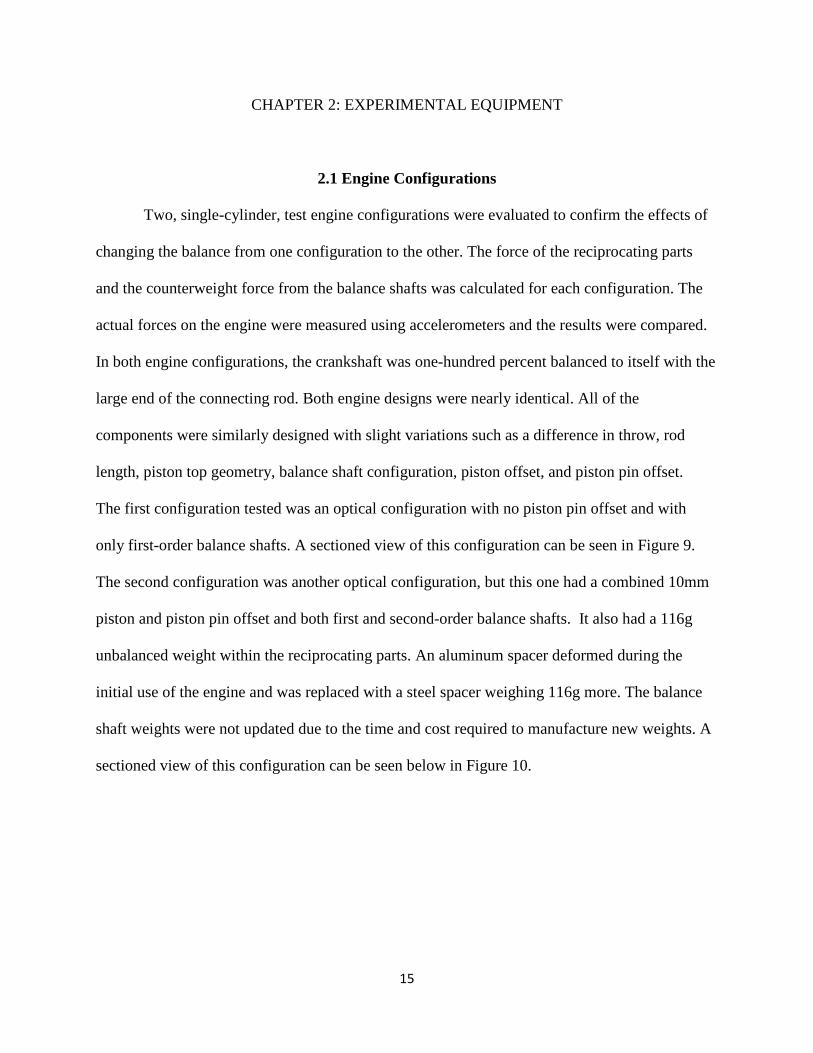
Two, single-cylinder, test engine configurations were evaluated to confirm the effects of
changing the balance from one configuration to the other. The force of the reciprocating parts
and the counterweight force from the balance shafts was calculated for each configuration. The
actual forces on the engine were measured using accelerometers and the results were compared.
In both engine configurations, the crankshaft was one-hundred percent balanced to itself with the
large end of the connecting rod. Both engine designs were nearly identical. All of the
components were similarly designed with slight variations such as a difference in throw, rod
length, piston top geometry, balance shaft configuration, piston offset, and piston pin offset.
The first configuration tested was an optical configuration with no piston pin offset and with
only first-order balance shafts. A sectioned view of this configuration can be seen in Figure 9.
The second configuration was another optical configuration, but this one had a combined 10mm
piston and piston pin offset and both first and second-order balance shafts. It also had a 116g
unbalanced weight within the reciprocating parts. An aluminum spacer deformed during the
initial use of the engine and was replaced with a steel spacer weighing 116g more. The balance
shaft weights were not updated due to the time and cost required to manufacture new weights. A
sectioned view of this configuration can be seen below in Figure 10.

16
Figure 9: Optical engine configuration with no piston pin offset and first-order balance shafts only.

17
Figure 10: Optical engine configuration with first and second-order balance shafts and piston offset.
2.2 Data Acquisition System and Sensors
2.2.1 Data Acquisition System
For the testing of the engines, an A&D Technologies Combustion Analysis System
(CAS) was used to capture the data. It is a high-speed data acquisition module that performs
online combustion analyses. It performs real-time, cycle-by-cycle calculations on combustion

18
data and processed data can be streamed to third party devices for closed loop control, or stored
to memory. User defined cycle-by-cycle calculations are supported, allowing the integration of
proprietary algorithms. Data can be set to acquire based on either crank-angle position or time.
The CAS system stores raw signals in memory and downloads the data to a computer for post-
processing using its own software. It has high speed analog inputs, digital inputs, analog outputs,
and digital outputs. The data acquisition rate is 2 MHz and the analysis rate without missing an
engine cycle is 1.2 MHz. Figure 11, below, shows an A&D CAS system.
Figure 11: A&D Technologies Combustion Analysis System (CAS)
2.2.2 Sensors
Two types of sensors were used to collect data during engine testing. The first sensor is
an accelerometer. The accelerometers that were chosen are top-mount, premium-grade
accelerometers from Omega Engineering. They feature a dynamic sensitivity of +/-5%:

19
100mV/g, acceleration range of 80g peak, and a frequency response of +/-5%. These
accelerometers only measure one direction, so three of them where used. The second sensor that
was used is an incremental, optical, rotary encoder. An incremental encoder produces a series of
square waves as it rotates. The encoder used, produces a wave pattern every degree of rotation
and another wave pattern every 360 degrees of rotation, or every full revolution. The encoder is
mounted on the crankshaft. This encoder provides information regarding the position and speed
of the crankshaft. These readings are used to correlate the data taken with the calculated,
unbalanced force.

20
CHAPTER 3: EXPERIMENTAL PROCEDURE
3.1 Computer-Aided Analysis and Calculations
3.1.1 Computer-Aided Crankshaft Design and Balance
Most manufactured parts are drawn using a 3-D modeling program at some point in the
design process. The 3-D model is used to create blueprints, run stress analysis and used to
compute other difficult computations quickly and easily. For balancing the crankshaft, a 3-D
modeling program was used to find the weights and centers of gravities within the crankshaft to
balance the crankshaft to itself. The crankshaft in an internal combustion engine is a complex
component. It requires intricate machining, and is highly stressed. Within the design of a
crankshaft there are many factors to consider, including bearing loads, oil film thicknesses,
cylinder pressures, rotating weights, and clearances with other parts, just to name a few. This
section focuses on some of the design parameters that are considered in just the balancing
portion of the crankshaft design.
In both of the research engines tested, the crankshaft is balanced with the heavy end of
the connecting rod and it is balance one-hundred percent to itself. When designing a crankshaft,
it should be designed in such a way that it is slightly overbalanced. Within the manufacturing
process a small amount of material will be removed in the final balancing process to achieve the
proper balance. It is always easier to remove material from the counterweights then to add it in
later. It is usually desired that the crankshaft should be 1.5 to 2 kg*mm overbalanced in the
design process to accommodate manufacturing variations (Ron Sears, personal interview,
February 5, 2014). The crankshaft will go through a final dynamic balance as the final step in the
manufacturing process that will remove the overbalance. Some of the parameters which can

21
greatly affect the balance of the crankshaft are, in order of most significant effect: the radius of
the counterweight (R), the thickness of the counterweight (T), the fan angle of the counterweight
(A), and an optional tungsten alloy slug added for additional counterbalance. These parameters
are depicted below in Figure 12. When calculating the effect of the tungsten slug, the weight
added will be the volume of the slug multiplied by the difference in the density between the
tungsten alloy and the steel used in the crankshaft.
Figure 12: Crankshaft design parameters to consider.
During the design process, the balance of the current computer model can be
mathematically calculated. The first step in this process is to divide the crank into sections which
consist of the counterweights, the cheeks, and the pins. Figure 12 depicts these divisions as
indicated by different colors. After the crank is divided into sections, the material properties are
applied within the model. Then, each section is analyzed to obtain the initial input data for the
calculations. The input data that is needed is the weight of each section and the center of gravity
locations in the X, Y, and Z planes shown in Figure 12. Once this data is obtained a table can be
created to organize the procedure. A sample can be seen in Table 2, below, where the areas
Z
T
X
Y
A
R
Slug

22
highlighted in green are the input data which consist of the weight (WR), the X locations of the
center of gravity (X), the Y locations of the center of gravity (Y), and then the Z locations of the
center of gravity (Z). The initial starting datum that the measurements are taken from should be
placed in the center of the first main bearing. The static balance calculation was then performed
by taking the weight (WR) of each part and multiplying it by the X and Y distances for each
component (see Equation 5 and 6). This data is recorded in the WR X, WR Y portion of Table 2.
𝑊𝑊 × 𝑋 = 𝑐𝑠𝑎𝑠𝑠𝑐 𝑝𝑐𝑟𝑠𝑠𝑐𝑝 𝑠𝑝 𝑋 (5)
𝑊𝑊 × 𝑌 = 𝑐𝑠𝑎𝑠𝑠𝑐 𝑝𝑐𝑟𝑠𝑠𝑐𝑝 𝑠𝑝 𝑌 (6)
The static portions in X of each component are summed and will, ideally, equal zero. The static
portions in Y are also summed and should be equal to zero. If the sums do not equate to zero, the
crankshaft should be altered, changing R, T, A, or adding a slug. It should be remembered that
the general condition of balance with numerous masses is that the vector sum of all the moments
equals zero. Along with being statically balanced, the crank also needs to dbe dynamically
balanced. Equations 7 and 8 can be used to find the dynamic portion of each component by
multiplying the static values by the Z distance of its center gravity.
𝑊𝑊 × 𝑋 × 𝑍 = 𝐷𝐷𝑝𝑎𝐷𝑠𝑐 𝑝𝑐𝑟𝑠𝑠𝑐𝑝 𝑠𝑝 𝑋 (7)
𝑊𝑊 × 𝑌 × 𝑍 = 𝐷𝐷𝑝𝑎𝐷𝑠𝑐 𝑝𝑐𝑟𝑠𝑠𝑐𝑝 𝑠𝑝 𝑌 (8)
These values are summed similarly to the static values. Both the static and dynamic calculations
should be figured at the same time and both should be equal to zero. To satisfy this condition, the

23
counterweight that is closest to the initial starting datum will be heavier than the counterweight
that is further away. Usually, the final balancing hole that is used to remove the slight
overbalance of 1.5-2 kg mm designed into the crank for machining variations is drilled in the
counterweight that is furthest from the initial starting datum. The crankshaft should always be
dynamically balanced on a crankshaft balancing machine to achieve the final balance of the part.
Equations 7 and 8 are used to guide the design of the crankshaft and make sure the crank is just
slightly over balanced so the balance machine will have to remove very little from the crank to
balance it.
Table 2: Static and dynamic balance calculations.
3.1.2 First and Second-order Balance Shafts
The MSU EARL team has designed and built numerous single cylinder test engines,
some with just first-order balance shafts and some with first and second-order balance shafts.
The balance shafts within these engines are designed so that the balance of the engine can be
changed as the configuration of the engine changes. This is done by designing the shafts with a
Wr X Y Wr X Wr Y Z CX CYkg mm mm kg mm kg mm mm kg mm2 kg mm2
Balance Hole 1 0.0000 0.0000 0.0000 0.0000 0.0000 38.3443 0.0000 0.0000Counterweight 1 1.8650 0.0348 -58.2207 0.0649 -108.5823 38.3443 2.4878 -4163.5146Cheek 1 2.7743 -0.0356 6.8137 -0.0986 18.9033 39.1488 -3.8619 740.0420Pin 1 1.2003 -0.0003 47.1528 -0.0003 56.5958 79.6191 -0.0249 4506.1057Est. Bob Weight 1 1.8820 0.0000 47.3000 0.0000 89.0186 79.3500 0.0000 7063.6222Oil Weight 0.0147 1.7614 28.2513 0.0258 0.4140 70.9334 1.8308 29.3638Counterweight 2 1.3790 0.0000 -55.2893 0.0000 -76.2440 120.3577 -0.0001 -9176.5508Cheek 2 2.7925 0.0000 7.1265 0.0000 19.9006 118.3353 0.0013 2354.9466Balance Hole 2 0.0000 0.0000 0.0000 0.0000 0.0000 120.3577 0.0000 0.0000
Component
= Static Balance = Dynamic Balance

24
bolt-on weight that can be taken on and off and changed as needed. Figure 13, below, represents
this design where the balance shafts are green and the removable weights are blue.
Figure 13: A computer generated model of the first-order (top) and second-order (bottom) balance shafts.
The purpose of the balance shafts is to generate a force equal to the reciprocating force, but in
the opposite direction. This is accomplished by using pairs of counter-rotating shafts: one pair
for the first-order force and one pair for the second-order force. The first-order shafts will rotate
at the same speed as the crank, and the second-order balance shafts will rotate at twice the speed
of the crank. Figure 14 illustrates this configuration and the forces within the engine. It also
shows the forces of each of the balance shafts along with the force of the recipricating parts. It
shows the rotation of the balance shafts, the axes that the forces act in, and the resultant moment
from the offset of the axes due to the piston and piston pin offset.

25
Figure 14: The rotation and forces within the engine at TDC
For any configuration, whether it be an optical Bowditch configuration or a standard
configuration, the weights for the balance shafts can be calculated. In the design process,
computer-aided models are analyzed to obtain weights of all of the reciprocating parts and the
balance shafts. The weights of the reciprocating parts are summed and then multiplied by the
throw to obtain the force of the reciprocating parts as demonstrated in equations 9 and 10.

26
𝐹𝑓𝑅𝑚𝑓𝑅 𝑅𝑚𝑜𝑜𝑚 = −𝐷𝜔2𝑟(𝑐𝑐𝑐(𝜃)) (9)
𝐹𝑓𝑜𝑠𝑅𝑅𝑜 𝑅𝑚𝑜𝑜𝑚 = �𝑚𝑅�𝐷𝜔2𝑟(𝑐𝑐𝑐(2𝜃)) (10)
In Equations 9 and 10, r is the rotational distance from the shaft centerline, ω is the angular
velocity (in radians per unit time), l is the length of the connecting rod, and θ is the crank angle
from TDC.
For the balance shafts, the mass of each shaft and its bolts is measured as is the distance
of the center of gravity to the axis of rotation. The force that the shaft will exert is equal to its
mass multiplied by the distance between the center of gravity and its axis of rotation. Table 3 is
used along with Equations 7 and 8, from above, to calculate the portion of the first-order and
second-order forces within it and helps organize the numbers. The first-order force of the
reciprocating parts is 49822.3 gr*mm and the first-order balance shaft force is 49814.8 gr*mm
giving a difference of 7.5 gr*mm. The second order force of the reciprocating parts is
15001.4gr*mm and the second order balance shaft force is 14993.8gr*mm giving a difference of
7.6 gr*mm. The sum of the differences is 15.1 gr*mm of residual imbalance, which is very low.
Within the table, the computer generated values are in blue and the measured values of the
manufactured, physical part are in yellow. The computer-generated numbers were used to get
preliminary drawings for the purpose of machining, but in the final calculations the measured
values of the physical part were used. It is helpful to examine both the computer generated value,
and the measured number together to recognize any variations that may indicate flaws or defects
within the computer-aided analysis, the part itself, or the fabrication process. The table below

27
demonstrates that the difference between the measured values and the computer-analyzed values
are almost identical, having a maximum difference of only six grams within any part.
Table 3: Balance shaft component values used in calculating the reciprocating forces.
3.1.3 The Connecting Rod
A portion of the weight of the connecting rod was used in both the crankshaft
calculations and the balance shaft calculations. For these calculations, the weight of the
connecting rod was sectioned into the large and small ends. The large end was used in the
crankshaft calculations because it rotates with the crank and the small end is used in the balance
shaft calculations because it reciprocates with the piston. The division line of the connecting rod
was identified as the center of gravity. All of the bolts and bearings were considered in the
calculations. Within the computer model, the center of gravity and weights of each component
were easily obtained. Figure 15 shows a model of a sectioned connecting rod.
Balance Shaft Components Weight (g) Weight (g)Center of Gravity
Offset (mm)1st order1st order balance shaft mass 5751.9 5751.6 18.71st order balance shaft bolts 236.1 230.9 17.71st order balance shaft top counterweight 3516.9 -24.72nd order 2nd order balance shaft 699.4 694.8 -0.42nd order balance shaft bolts 59.6 59.6 7.82nd order balance shaft counterweight 720.9 10.1
= Computer-Analyzed Data = Physically Measured Data

28
Figure 15: An example model of a connecting rod that is sectioned for analysis.
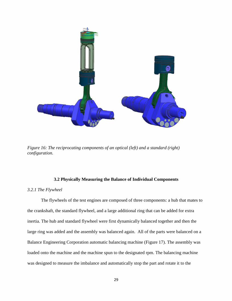
3.1.4 Reciprocating Parts
All of the reciprocating parts were analyzed within the model for the balance shaft weight
calculations. The reciprocating components of the standard configuration consist of the small end
of the connecting rod, the piston pin, the piston, and the piston rings. For an optical
configuration, the reciprocating components consist of the small end of the rod, the piston pin,
base piston, base piston rings, Bowditch piston extension, Bowditch piston bolts, Bowditch
piston top, Bowditch piston rings, an optical window, and seals for the optical window. Figure
16 shows a computer-generated model depicting the standard and optical configurations of the
reciprocating components.
29
Figure 16: The reciprocating components of an optical (left) and a standard (right) configuration.
3.2 Physically Measuring the Balance of Individual Components
3.2.1 The Flywheel
The flywheels of the test engines are composed of three components: a hub that mates to
the crankshaft, the standard flywheel, and a large additional ring that can be added for extra
inertia. The hub and standard flywheel were first dynamically balanced together and then the
large ring was added and the assembly was balanced again. All of the parts were balanced on a
Balance Engineering Corporation automatic balancing machine (Figure 17). The assembly was
loaded onto the machine and the machine spun to the designated rpm. The balancing machine
was designed to measure the imbalance and automatically stop the part and rotate it to the

30
position were a balancing hole needs to be placed then commence to automatically drill the hole,
or holes, if more than one is needed.
Figure 17: Balance Engineering Corporation automatic balance machine.
3.2.2 The Crankshaft
Each crankshaft is dynamically balanced as the final step in the manufacturing process.
To balance the crank, the mass of the large end of the rod must be known and a bob weight of the
same mass as the connecting rod must be placed onto the pin of the crank. The crankshaft is
mounted into the balancing machine (Figure 18) with the bob weights attached, and the locations
of the counterweights are input into the machine. The balancing machine will then spin the
crankshaft and measure the balance of the crank. It will then rotate the crank to the location of
the counter-balance hole locations and indicate the amount of correction that is needed. Material
is then added or removed, as indicated, to achieve proper balance.

31
Figure 18: Crankshaft balancing machine.
As a check, or if the crank, and/or the reciprocating mass, is modified after the
manufacturer’s dynamic balance process, the crankshaft can be statically balanced using a stand,
like that in Figure 19, that is designed to allow for the crankshaft to rotate freely when mounted.
The stand usually consists of large wheels mounted on smooth operating bearings. The proper
bob weight will be attached to the pin. If the crankshaft is balanced, it will not rotate when it is
placed onto the stand. If it does rotate, then the heavier end will rotate to the bottom. If the pin
side is heavy, the counterweights will be increased. If the counterweight is heavy, weight will
remove from the counterweight in the direction of the vector that is pointing directly downward.
This technique can only be used with crankshafts that are one-hundred percent balanced to

32
themselves. To identify the mass to be removed or added the balance refers to the calculations
discussed in section 3.1.1.
Figure 19: Crankshaft mounted on a static balance stand.
3.3 Parts are Physically Measured to Verify Accuracy
3.3.1 The Connecting Rod
There are a several techniques used to check the weight and balance of the connecting
rod. It is always good to weigh every part that is going to be rotating or reciprocating and
compare it to the weight generated by the computer-aided analysis to ensure that they agree. If
there are any discrepancies, the cause of the discrepancies should be investigated and corrected.
Since the center of gravity serves as the separation point between the large and small ends, the

33
center of gravity location must be identified and compared to the computer-analyzed position. To
find the center of gravity, the connecting rod can be balanced on a pin or blade. The pin position
can then be marked on the connecting rod and it can then be measured to verify that it is in the
proper location according to the computer-generated data. Figure 20 shows a picture of a
connecting rod mounted on a mill to measure the mark made by balancing it on a pin. The
position determined by this method was within 0.02 inches from the position calculated from the
3-D computer solid modeling program.
Figure 20: A Connecting rod mounted on a mill to measure the mark made by balancing it on a pin.
Another way of confirming the large end and small end weights of the connecting rod is
to place the connecting rod in a fixture the will allow it to be truly horizontal, and have one end
of the rod suspended while the other end is placed on a scale and can be measured. This method

34
is widely used by performance shops because it is an inexpensive and simplistic way to obtain
both the large and small end weights. A picture of this setup can be seen below in Figure 21. For
one of the connecting rods used in one of the engines, the computer analyzed weight of the large
end was 1015.9 grams, the small end was 657.5 grams, and the total was 1673.4 grams. For the
same connecting rod, the physically measured weight for the large end was 1262.4 grams, the
small end weighed 411.4 grams, and the total weight was 1673.0 grams. Measuring both ends
separately and them combining them, produced a total weight of 1673.8 grams. There was a 0.8
gram discrepancy between this value and the value obtained measuring the weight of the
connecting rod as a whole, and a 0.4 gram difference from the total weight determined by the
computer analysis of the 3-D model. Both methods result in values that agree quite well and the
slight discrepancy is negligible. Investigating the weight of the large end of the rod, 1015.9
grams for the computer analyzed weight and 1262.4 grams for the measured weight, there is a
large difference between how each method distributes the weight between the large end and
small end. For all of the balancing of the other engine components, where either the small end or
large end weights are needed, the computer-analyzed weights were used. The computer-analyzed
weights were used because, in the design process, these weights are needed for the design of the
crankshaft and balance shafts.

35
Figure 21: A connecting rod being weighed to find the large and small end weights.
3.3.2 The Balance Shafts and Weights
For validation, any reciprocating or rotating part was weighed and compared the
computer-analyzed weight of the model. All of the components of the balance shafts went
through this process. The balance shafts themselves, the balance shaft weights, the bolts, and the
keyways are measured with the shafts assembled and then again once they are dismantled. If
there are any discrepancies between the physically measured value and the computer-analyzed
value, the part is assessed and any necessary modifications are made. A high-precision scale is
used to collect the physical measurements of the weight of each component.

36
CHAPTER 4: TESTING
4.1 Testing Procedure
A dynamometer was connected to the engine to motor the engine for testing. The engine
was run from 300 RPM to 2000 RPM in increments of 50 RPM. At each speed, the engine was
motored until the set speed had been reached and was stabilized. Data was then captured from
three accelerometers mounted to the crankcase in the X, Y, and Z directions of the engine. The Z
direction was in the axis of reciprocation. The Y direction was in the axis of crank rotation. The
X direction is perpendicular to the engine’s side. The connecting rod rotates in the X-Z plane.
Data was taken for 15 seconds at a data capture rate of 50 kHz using time-based data acquisition
with a 25 kHz cut-off filter. After all of the data points had been captured, the data was then run
through Matlab and Fast Fourier Transform (FFT) and plots were obtained. The FFT plots were
then assembled into a Campbell diagram for further data analysis. Combustion data was also
taken in a similar manner at 1500 RPM and 2000 RPM.
The first configuration test engine was run at 800, 1000, 1500, and 2000 RPM. At each
speed, the engine was motored until the set speed had been reached and was stabilized. Data was
then captured from three accelerometers mounted to the crank case in the X, Y, and Z directions
of the engine. The Z direction was in the axis of reciprocation. The Y direction was in the axis of
crank rotation. Data was taken crank-angle based, taking a data point at each degree of rotation
of the crankshaft. For each speed the data capture rate is different due to how the data was
captured. The data capture rate for 2000 RPM works out to be 12 kHz and would be slower for
the slower speeds. The data was processed similarly as that of the second configuration test
engine through Matlab to obtain FFT plots.

37
4.2 Fast Fourier Transform (FFT)
Through FFT, time-based data is converted into frequency-based data. The Fourier
Transformation takes any complex signal and breaks it down into an infinite number of distinct
frequency sine waves having different magnitudes. Below, in Figure 23, both the time-based data
and its frequency-based response can be seen. From the frequency response, it can be observed
that the time-based data is made up of two sine waves at different frequencies and two different
magnitudes. The sum of these two sine waves will produces the complex time-based signal. The
FFT allows for the collection of a time-based signal and calculates the frequencies and
magnitudes of the sine waves that are apparent in the time-based data.
Figure 22: The top graph represents a complex time-based signal, and below it is a FFT graph showing that the complex signal can be broken into two different sine waves of differing frequency and magnitudes. Reprinted from Fast Fourier Transform in Wikipedia (2014), Retrieved November 18th, 2014 from http://en.wikipedia.org/wiki/Fast_Fourier_transform.

38
4.3 Campbell Diagram
A Campbell diagram is a 3-D plot that shows the frequency versus speed versus
magnitude of the frequency. Campbell diagrams are commonly used in rotational systems to
analyze critical frequencies, wearing parts, failure modes, and natural harmonics within a system.
For example, within turbines and turbo machinery, the flex and vibration of the turbine blades
can be analyzed. Using a Campbell diagram to investigate a gear box reveals gear interactions,
gear damage, gear wear, and bearing failure. In all cases, natural harmonic frequencies will also
be easily identified with the Campbell diagram. Campbell diagrams show order lines which
represent the reaction of the system to some event related to the rotation of the device. As the
rotational speed increases, so will the frequency at which the event takes place. Figure 24 depicts
an example of a Campbell diagram. The order lines through the graph that increase in frequency
as speed increases can be seen as a light line compared to its surroundings. The order of each line
is labeled on the right side of the graph. The magnitude of the event is color coded from blue to
red; the higher the magnitude of the response, the deeper red it will become. The vertical areas or
lines at certain frequencies are the natural frequencies of the system. They occur at 210 Hz, 300
Hz, 510 Hz, 1140 Hz, and 1440 Hz. The interaction of the orders with the natural frequencies
can be viewed as the natural frequency lines cross order lines. The orders that will excite the
natural frequency more than others can be identified as the higher magnitude areas. The fourth
order excites the 300 Hz natural frequency more than the other orders. From this data, the system
can be either redesigned to change the factor that corresponds with the fourth order event, the
system can be operated in a way to stay below the 300 Hz natural frequency, or the time that the
engine operates within that region can be minimalized.

39
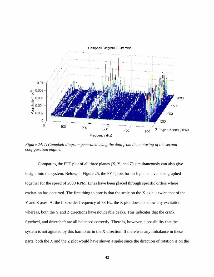
Figure 23: An example of a Campbell diagram showing order lines, natural frequencies, and their interaction. Reprinted from Campbell Diagram, Bing Images (n.d.) Retrieved November, 2014 from http://www.mnoise-software.com/References.3908.0.html Copyright 2014 by Engineering Center Steyr. Reprinted with Permission.

40
CHAPTER 5: RESULTS AND DISCUSSION
5.1 Second Configuration Test Engine Motoring Results
The research relayed in this publication was performed to investigate the reaction of the
system to the addition of second order balance shafts into a single-cylinder optical engine. The
response of the engine was captured using accelerometers. The accelerometers show the reaction
of the system from the point on the engine to which they are mounted. One of the most effective
ways to illustrate these results is to display them in a Campbell diagram. Below, in Figure 24, a
Campbell diagram of the reciprocating axis, the Z direction, is shown.
It is important to identify the natural frequencies of the system so that these ranges can be
avoided in the operation of the engine. These frequencies can be identified easily within the
Campbell diagram and are represented by vertical lines running through the diagram. The natural
frequencies of the system between 0 and 500 Hz are: 60 Hz, 115 Hz, 172 Hz, 187 Hz, 230 Hz,
350 Hz, 457 Hz, and 470 Hz. The harshness of each natural frequency is shown by the
magnitude of the line. The natural frequencies at 457 Hz and 470 Hz are more severe than the
other natural frequencies within the system.
The first and second-order effects within the engine are of the most interest. Within the
Campbell diagram, the order effects can be seen as lines running at an angle through the
diagram. The lower orders start on the left side of the diagram and are nearly vertical at this
initial point. As the order increases, the order lines become more horizontal. Three orders can be
seen in the motoring results of the second configuration test engine through the entire speed
range. These orders are the first-order, second order, and the 5.5 order. At speeds above 1500
RPM, the third order, fourth order, eighth order, and tenth order also begin to show up within the

41
Campbell diagram. The order lines can be identified by looking at the ending frequency of the
line at 2000 RPM. The first order frequency is 33 Hz, second order is 66 Hz, third order is 100
Hz, fourth order is 133 Hz, five and half order is 183 Hz, eighth order is 266 Hz, and the tenth
order is 333 Hz.
The first and second order lines indicate that the magnitude of the response increases with
speed. This implies the presence of an unbalanced mass within the reciprocating parts. For this
configuration there was a 116 g mass within the reciprocating parts that was not balanced by the
balance shafts. This response within the Campbell diagram is due to the rotational speed,
specifically the 𝜔2 term, of the force calculation. For the 5.5 order, the response had the same
magnitude over the full speed range from 300 RPM to 2000 RPM. Through the process of
investigating all of the rotating parts, such as the balance shafts, crankshaft, flywheel, driveshaft,
gears within the geartrain, and bearings, it was discovered that the bearings containing 11 ball-
bearings that were used in four locations in the engine, all rotated at half the frequency of the
crankshaft rotation giving a 5.5 order effect. Two of these bearings were located in the
distributor shaft housing and two more were located in the jack shaft housing. This 5.5 order
frequency showed up in all three planes, and this prevalancy may be due to the fact that the
accelerometers were mounted very near the locations of the bearings. The bearings should be
monitored by re-running the same test and comparing the magnitudes of the response for this
order. If the magnitude of the 5.5 order increased, this would indicate that one of the bearings is
failing and should be replaced. The fourth order excites the harmonic at 115 Hz along with the
eighth order exciting the harmonic at 230 Hz at around 1800 RPM. This is represented by the
very high peak magnitudes within the Campbell diagram.
42
Figure 24: A Campbell diagram generated using the data from the motoring of the second configuration engine. Comparing the FFT plot of all three planes (X, Y, and Z) simultaneously can also give
insight into the system. Below, in Figure 25, the FFT plots for each plane have been graphed
together for the speed of 2000 RPM. Lines have been placed through specific orders where
excitation has occurred. The first thing to note is that the scale on the X-axis is twice that of the
Y and Z axes. At the first-order frequency of 33 Hz, the X plot does not show any excitation
whereas, both the Y and Z directions have noticeable peaks. This indicates that the crank,
flywheel, and driveshaft are all balanced correctly. There is, however, a possibility that the
system is not agitated by this harmonic in the X direction. If there was any imbalance in these
parts, both the X and the Z plot would have shown a spike since the direction of rotation is on the

43
X-Z plane. Some effect at the first-order frequency from the moment created by the piston and
piston pin offset within the X direction would also be expected in the presence of any imbalance.
Since there is no noticeable effect in the X direction, it can be assumed that the moment did not
have a significant effect on the system. Within the plots, the order harmonics, and also the
natural frequency harmonics of the system can be seen. Looking at just the FFT plot without a
Campbell diagram, it is harder to distinguish between order harmonics and natural frequency
harmonics because both harmonics look the same. Using both the FFT plot and the Campbell
diagram together, it is easy to identify the harmonics and to find the values of each peak.
Figure 25: A FFT Plot generated using the data from the motoring of the second configuration test engine at 2000 RPM.
5.2 Second Configuration Test Engine Firing Results
The reaction of the system due to the combustion event within the engine was
investigated. In Figure 26, FFT plots for each direction have been graphed together for the speed
of 2000 RPM at which combustion was occurring. It can be determined, by comparing Figure 25
1 2 3 5.5 8 10

44
and Figure 26, that each of the magnitudes in the combustion data increased by an order of
magnitude. This excitation in the magnitudes may be due to the torque change caused by the
pressure created in the cylinder by combustion. There is also a half-order spike at 16 Hz that
represents the combustion event that occurs once every two revolutions.
Figure 26: A FFT Plot generated using the data from combustion testing of the second configuration test engine at 2000 RPM.
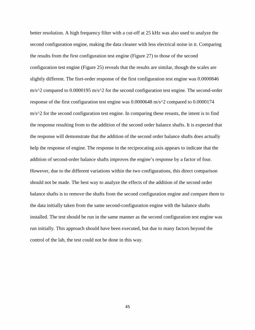
5.3 First Configuration Test Engine Motoring Results
The main differences between the data taken from the first configuration test engine and
the second configuration test engine are due to the fact that the first configuration test engine
does not have second-order balance shafts. Also, the data was captured in a different way. The
data in the first configuration test engine was captured crank-angle based, and the data captured
in the second configuration test engine was time-based. The data captured within the second
configuration test engine was also taken at a higher data capture rate, which produced results at a
45
better resolution. A high frequency filter with a cut-off at 25 kHz was also used to analyze the
second configuration engine, making the data cleaner with less electrical noise in it. Comparing
the results from the first configuration test engine (Figure 27) to those of the second
configuration test engine (Figure 25) reveals that the results are similar, though the scales are
slightly different. The fisrt-order response of the first configuration test engine was 0.0000846
m/s^2 compared to 0.0000195 m/s^2 for the second configuration test engine. The second-order
response of the first configuration test engine was 0.0000648 m/s^2 compared to 0.0000174
m/s^2 for the second configuration test engine. In comparing these resusts, the intent is to find
the response resulting from to the addition of the second order balance shafts. It is expected that
the response will demonstrate that the addition of the second order balance shafts does actually
help the response of engine. The response in the reciprocating axis appears to indicate that the
addition of second-order balance shafts improves the engine’s response by a factor of four.
However, due to the different variations within the two configurations, this direct comparison
should not be made. The best way to analyze the effects of the addition of the second order
balance shafts is to remove the shafts from the second configuration engine and compare them to
the data initially taken from the same second-configuration engine with the balance shafts
installed. The test should be run in the same manner as the second configuration test engine was
run initially. This approach should have been executed, but due to many factors beyond the
control of the lab, the test could not be done in this way.

46
Figure 27: A FFT plot generated using the data from the motoring of the first configuration test engine at 2000 RPM.
1 2

47
CHAPTER 6: CONCLUSIONS
Within this publication, both analytical and physical processes to balance the components
within a single cylinder engine have been identified and discussed. These processes can also be
expanded to be used in multi-cylinder engines. Also, a test procedure has been developed to
evaluate the dynamic response of a single-cylinder test engine along with data processing
techniques that can be used to clearly display the data.
From this research the following conclusions have been reached:
1. The natural frequencies of the second configuration test engine system, between 0 and
500Hz, are: 60 Hz, 115 Hz, 172 Hz, 187 Hz, 230 Hz, 350 Hz, 457 Hz, and 470 Hz.
2. Within the second configuration test engine, the response of the following order
harmonics that are present at 2000 RPM between 0 and 500 Hz have been identified to
be: first order (33 Hz), second order (66 Hz), third order (100 Hz), fourth order (133 Hz),
five and one-half order (183 Hz), eighth order (266 Hz), and tenth order (333 Hz).
3. Noise from the bearings have been identified and could be a sign of initial bearing failure
and should be monitored for replacement.
4. The first and second-order responses of the system are low, utilizing the bearing noise
response as an indicator. The response of the bearing noise within the system should be
very small.
5. The balance of the crankshaft, flywheel, and driveshaft is excellent and the procedure for
dividing the connecting rod within a 3-D model is very effective.
6. Combustion within the second configuration test affects the vibrational response of the
system dramatically.

48
7. The response of the system from the moment created by a combined piston and piston pin
offset of 10mm, within the second configuration test engine, is minimal.

49
CHAPTER 7: RECOMMENDATIONS
There are several other topics that would be interesting to study that are related to this
research. One of which would be the effects of the head on the vibration of the engine. The head
has several moving parts, including valves and camshafts. In high-performance engines it is
becoming popular to also balance the camshafts. This test could be performed by disconnecting
the drive belt from the head in either test configuration engine. Another interesting topic that
arose during this research was how the connecting rod weight is split between the large end of
the rod the small end of the rod. Several engine shops that balance crankshafts were contacted
and they primarily use the physically measured values discussed in 3.3.1, but after performing
the physical measurements it was discovered that there was a large difference in the weight
distribution between the large end and the small end relative to the 3-D analyzed weight
distribution. For the experiments in this publication, the 3-D analyzed weight distribution was
used and the results were excellent. To complete this experiment, the crankshaft would have to
be re-balanced and new balance-shaft weights would have to be manufactured for one of the test
engines. Analyzing the response due to the addition of the second order balance shafts within the
second configuration by first removing the shafts and running the same initial test would be very
beneficial to this research. For any future engine designs that have piston offset or piston pin
offset, the balance shafts should be placed directly under the cylinder so that the moment
discussed in 3.1.2 is not created.

50
REFERENCES

51
REFERENCES
Dynamic Balance. (2003). The Free Dictionary. Retrieved November, 2014 from http://encyclopedia2.thefreedictionary.com/dynamic+balance
Foale, Tom. (2007). Some Science of Balance. Retrieved from http://www.tonyfoale.com/Articles/EngineBalance/EngineBalance.pdf Hoag, Kevin. (2006). Engine Configuration and Balance. In Vehicular Engine Design (Ch. 6).
Retrieved from http://link.springer.com/chapter/10.1007/3-211-37762-X_6#page-1 Sharp, Archibald. (1907). Balancing of Engines Steam, Gas, and Petrol: An Elementary Text-
Book, Using Principally Graphical Methods, for the Use of Students, Draughtsmen, Designers and Buyers of Engines. Retrieved From https://play.google.com/store/books/details/Archibald_Sharp_Balancing_of_Engines_Steam_Gas_and?id=ekYKAAAAIAAJ