Dual Virtual Element Methods for Discrete Fracture MatrixmodelsAlessio Fumagalli*, and Eirik Keilegavlen

Department of Mathematics, University of Bergen, 5007 Bergen, Norway

Received: 5 December 2017 / Accepted: 6 February 2019

Abstract. The accurate description of fluid flow and transport in fractured porous media is of paramountimportance to capture the macroscopic behavior of an oil reservoir, a geothermal system, or a CO2 sequestra-tion site, to name few applications. The construction of accurate simulation models for flow in fractures ischallenging due to the high ratio between a fracture’s length and width. In this paper, we present a mixed-dimensional Darcy problem which can represent the pressure and Darcy velocity in all the dimensions,i.e. in the rock matrix, in the fractures, and in their intersections. Moreover, we present a mixed-dimensionaltransport problem which, given the Darcy velocity, describes advection of a passive scalar into the fracturedporous media. The approach can handle both conducting and blocking fractures. Our computational gridsare created by coarsening of simplex tessellations that conform to the fracture’s surfaces. A suitable choiceof the discrete approximation of the previous model, by virtual finite element and finite volume methods, allowsus to simulate complex problems with a good balance of accuracy and computational cost. We illustrate theperformance of our method by comparing to benchmark studies for two-dimensional fractured porous media,as well as a complex three-dimensional fracture geometry.

1 Introduction

Fractures and faults can strongly influence fluid flow in aporous media, acting, depending on their permeabilityand porosity, as a preferential path or a barrier. As fractureaperture is several orders of magnitude smaller than anyother characteristic size in the domain, fracture modelingis one of the main challenges in subsurface problems.

Geological movements, chemical reaction, or infillingprocesses may substantially alter the local orientation andcomposition of the material present in the fractures, leadingto anisotropies and strong heterogeneities in both fracturesand their intersections. It is thus crucial to be able toinclude also these phenomenological aspects in the concep-tual model.

Applications where fractures can be determinant forreservoir behavior include exploitation of geothermal sys-tem, CO2 storage and sequestration, enhanced oil recovery,and nuclear waste disposal. In these fields the solution maydramatically depend on the presence of fractures, thus acorrect derivation of suitable mathematical models andtheir accurate numerical solution is essential.

Our computational model is based on a DiscreteFracture Matrix (DFM) approach, e.g. [1], which aims to

balance computational cost and modeling accuracy in thepresence of fractures on multiple scales. Small scalefractures are incorporated in the matrix permeability byanalytical or numerical upscaling techniques (e.g. see [2–4]and [5–7]), thus only macroscopic fractures and faults areconsidered and explicitly described. However, thecomputational cost associated with their equi-dimensionalrepresentation in the grid is still prohibitively high. Follow-ing the idea presented, among the others, in references[8–15] fractures and faults are represented as lower-dimen-sional objects embedded in the rock matrix. This approachis commonly denoted reduced models, hybrid-dimensionalmodels, and mixed-dimensional models. In this approach,fracture aperture becomes a coefficient in the equations,instead of a geometrical constraint for grid generation.The flow equations are averaged along the normal directionof the fractures, yielding a new set of reduced modelsthat are suited for the co-dimensional, that is, lower-dimensional, description of fluid flow. Suitable couplingconditions are necessary to exchange information betweenall the objects (rock matrix, fractures, and theirintersections).

The reduction of dimensionality is an essential step toovercome most of the difficulties associated to the problem.However, in the presence of several fractures that togetherform a complex network, more advanced numerical* Corresponding author: alessio.fumagalli1984@gmail.com

This is an Open Access article distributed under the terms of the Creative Commons Attribution License (http://creativecommons.org/licenses/by/4.0),which permits unrestricted use, distribution, and reproduction in any medium, provided the original work is properly cited.

Oil & Gas Science and Technology - Rev. IFP Energies nouvelles 74, 41 (2019) Available online at:�A. Fumagalli & E. Keilegavlen, published by IFP Energies nouvelles, 2019 ogst.ifpenergiesnouvelles.fr

https://doi.org/10.2516/ogst/2019008

Numerical methods and HPCA. Anciaux-Sedrakian and Q. H. Tran (Guest editors)

REGULAR ARTICLEREGULAR ARTICLE

techniques are crucial to obtain an accurate solution in areasonable amount of time. The main aspect is the geomet-rical treatment of the fracture grid with respect to the rockmatrix grid. Popular approaches can be classified accordingto whether the grid in the rock matrix matches the fracturesurfaces or not. The matching case can further be split intomethods that assume full conformity between the rockmatrix and fracture grid, and methods that relaxe thisassumption.

In the class of conforming methods, where fracture gridsare composed by faces of the rock matrix grid, severalnumerical schemes have been considered, including finiteelements [13, 16–19], finite volumes [6, 20–23], MimeticFinite Differences (MFD) [24, 25], and the newly introducedVirtual Finite Elements (VEM) [26–28]. For the latter seealso [29–33] for the non-fractured case. All these methodshighlight specific advantages for example related to localmass conservation, capability to be implemented in stan-dard software packages, or relax some constraints on gridcell shapes to name a few.

In the class of non-conforming discretization, the maintool is a mortar coupling between the rock matrix gridand the fracture grids. The rock mesh is constrained withthe position of the fractures but not strictly with the actualfracture meshes, and vice versa. Some examples arereported in [10, 27, 34] where different type of mortarvariables as well as numerical schemes are considered. Themortar variables allow for a generalized formulation thatunifies conforming and non-conforming approaches [35].

Finally, a fully non-matching coupling among the gridsrequires ad-hoc solutions to establish a communicationbetween the fractures and the rock matrix. One possibilityis the class of eXtended Finite Element Methods (XFEM)[36–41], where a local enrichment with new basis functionsis considered to handle the non-conformity, or the class ofEmbedded Discrete Fracture Matrix Methods (EDFM)[5, 41–43], where approximate formulas for fracture-matrixtransmissibilities are computed based on geometricalconsiderations.

In this paper we consider a conforming discretizationwith the dual virtual element approximation to simulate amixed-dimensional Darcy problem and a finite volume dis-cretization for the mixed-dimensional transport problem.The first choice is motivated by the flexibility of the VEMswith respect to the shape of the grid cells. With this choice itis possible to relax most of the difficulties related with con-forming discretization, e.g. the computational cost associ-ated to resolve, by the rock matrix grid, a complex systemcomposed of several intersecting fractures. Moreover, thisapproximation ensures local mass conservation and is ableto consider heterogeneous and anisotropic permeabilitytensors. The Darcy velocity can thus be used in the mixed-dimensional transport problem. In this case we consider anupwind scheme, extended to handle the mixed-dimensionalnature of the problem.

The paper is structured as follows: In Section 2, we pre-sent both the physical equations and the reduced model,with the interface conditions that couple the matrix-fracture system and the fracture-fracture system for boththe Darcy and transport problems. Section 3 deals with

the weak and integral formulation of the previous physicalprocesses. In Section 4, we present the numerical discretiza-tion of the problem with a highlight on the enrichment ofthe finite element spaces. In Section 5, we present somenumerical experiments to assess the effectiveness of theproposed method. Finally, Section 6 is devoted to conclu-sion and to ongoing work.

2 Mathematical model

In this section, we introduce the mathematical models inthe mixed-dimensional setting, i.e. equations that coupledifferent spatial dimensions and together describe the quan-tities of interest. We present two mathematical modelsuseful for subsurface simulations: the mixed-dimensionalDarcy problem, presented in Section 2.1, to describe theflow and pressure, and the mixed-dimensional transportproblem, presented in Section 2.2, to describe the motionof a passive scalar transported by the Darcy velocity.

The motivation for the mixed-dimensional formulationis the observation that the fracture aperture is orders ofmagnitude smaller than other characteristic sizes of theproblem. Hence, a straightforward mesh construction withthe two fracture surfaces as constraints would produce highnumbers of cells and/or low-quality cells due to high aspectratios or sharp angles. To avoid this geometrical constraint,fractures are represented as lower dimensional objectsembedded in the rock matrix. Fracture intersections, andtheir intersections again, are considered as objects of evenlower dimensions. To be specific, in a three-dimensionaldomain, we consider fracture surfaces as 2d objects, theintersection between two (or more) fractures form a 1d line,and two (or more) intersection lines can meet in a 0d point.The physical processes are described via reduced modelswith suitable coupling conditions among the objects ofdifferent dimensions. The fracture aperture is now part ofthe equations and not any more a geometrical constraint.For more details on the derivation of the reduced modelwe refer to [8–11, 13, 26–28, 37, 39, 40, 44, 45].

In the reduced model, it is a common choice to considerthe reduced scalar variables as averaged and the vectorvariables as integrated along cross section of the fracture.In this work we follow this approach.

In the sequel we indicate by (�,�)A the scalar product inL2 (A). Moreover, the trace operator on a domain A will beindicated by �|A.

2.1 Mixed-dimensional Darcy problem

Let us consider a regular domain X � RN , for N > 0, withouter boundary @X. The domain X is composed by a single,possibly non-connected, equi-dimensional domain XN andseveral lower-dimensional domains Xd for d < N, whichare possibly non-connected. Clearly [d=0,. . .,N Xd ¼ X andXd \ Xd 0 = ; for d 6¼ d 0. However, we indicate withCd = @Xd \ Xd�1, which is geometrically equivalent toXd�1 but it will be more convenient to keep them separate.We have C = [d=0,. . .,N Cd. See Figure 1 as an example ofthe subdivision.

A. Fumagalli and E. Keilegavlen: Oil & Gas Science and Technology - Rev. IFP Energies nouvelles 74, 41 (2019)2

We are interested in the mixed-dimensional Darcy prob-lem which describes the pressure and velocity fields in X.Following the idea presented in [10], we define the pressurecompound p = (p0, . . ., pN) which represents the pressure ineach dimension, indicated as superscript. Similarly, weintroduce the velocity compound u = (0, u1, . . ., uN, 0),which is the velocity field defined in XN or in the tangentialspaces of each dimension d < N. The meaning of the two 0 swill be clarified below. In the following problem, eachdimension is coupled with the lower dimension; we considerthus two normals n associated to a d< N-dimensional man-ifold with respect to its “two sides’’, indicated by n+ andn�. Each disconnected object with dimension d < N whenimmersed in the surrounding d + 1-manifold, it is assumedto be an orientable d-dimensional manifold, with uniquenormal n lying on the tangent space of the d + 1-manifold.This implies n+ = �n�, an illustration is given in Figure 2.In the particular case of T-type intersection only one sidecan be defined and the following equations should be under-stood in this sense. Given a side, by convention the normalvector points from the higher dimensional to the lower-dimensional domain. Moreover, we indicate by the samesubscript �± the restriction of elements in Xd defined on eachside of Cd through a suitable trace operator.

2.1.1 Fixed-dimensional Darcy problem

We consider the Darcy problem for the pressure andvelocity as

u þ Krp ¼ 0

r � �u � su � nt ¼ �finX: ð1aÞ

The � notation means “on the higher dimensional object”and the �� means “on the lower dimensional object”, i.e. fix adimension d the second of (1a) becomes

r � ud � sudþ1 � ndþ1t ¼ f d 0 � d � N :

In the system (1a) thefirst equation and second equations aredefined on domains of the same dimension. For lower dimen-sional objects, the differential operators are defined in thetangent plane of the objects; in the special 0d case theseobjects are void.K represents the effective permeability com-poundK= (1,K1, . . ., KN), which is a collection of symmet-ric and positive defined tensors. For d< N,Kd is interpretedas laying in the tangent plane of the relevant physicalobject. Model (1a) allows for permeability variations both

between all objects considered, and spatially within eachobject. The permeabilities are scaled by the “aperture” ofeach dimension: Denote by �d the length (N � 1), area(N � 2), or cross-sectional volume (N � 3). The permeabil-ity of a lower d-dimensional (d < N) object is then definedas Kd ¼ �d eKd , with eKd the permeability of its equi-dimen-sional representation. The unit of measure of Kd is thus[m4�d/s]. The source or sink term f is defined as the com-pound f = (f 0, . . ., f N), which are scalar functions definedin each dimension. Finally, the jump operatorsu � nt ¼ P

�u � nj� is imposed on each side of Xd�1

viewed as immersed in Xd.The first equation in (1a) is the generalized Darcy law in

each dimension, note that for the 0d case it is simply anidentity. The second equation of (1a) represents conserva-tion of mass: The divergence term prescribes conservationof mass within the dimension, while the jump term repre-sents the inflow/outflow from the higher dimension.Interaction with the lower dimension is incorporated intothe boundary conditions, see Section 2.1.3. Due to the def-inition of the velocity compound, for d = N equation (1a)the inflow/outflow from the “higher dimension” is null.For d = 0 the conservation of mass equation representsthe continuity of the fluxes for the 1-dimensional objectsinvolved in the intersection.

We emphasize that the mixed-dimensional problem onlyconsiders direct interaction between objects one dimen-sion apart. That is, quantities defined on Xd�1 are in com-munication with the quantities defined on Xd, but notdirectly with quantities defined on Xd+1.

2.1.2 Flow between dimensions

The coupling conditions between two subsequent dimen-sions are defined for each side as

u � nj� þ k� �p � pj�Þ ¼ 0 onC :ð ð1bÞThe k� is the effective normal permeability, defined ask� ¼ ðk0�; . . . ; kN�1

� Þ. Clearly, equation (1b) is validbetween dimension d and d + 1 for 0 � d < N. Note thatin equation (1b) it is possible to define different effectivenormal permeability on each side ±, however, to simplifythe notation, we assume only one single value.

(a) (b)

(c)

Fig. 2. Representation of the fracture normal associated withrespect to each “side” (+ and �). (a) A bidimensional domain X2,(b) The fracture is fictitiously enlarged. (c) For a 0d intersection.

Fig. 1. Domain subdivision for N = 2. In gray X2, in red X1, andin blue X0.

A. Fumagalli and E. Keilegavlen: Oil & Gas Science and Technology - Rev. IFP Energies nouvelles 74, 41 (2019) 3

2.1.3 Boundary conditions

To obtain a well-posed problem, boundary conditions mustbe assigned on the external boundary @X and the boundaryof the sub-domains of each dimension, Xd. We indicate byoXd

out the (possibly empty) portion of the boundary of Xd

that intersects the boundary of X, for d > 0. We introducealso oXd

in the portion of boundary of Xd that does not inter-sect with @X, for d > 0. oXd

in is further split into the internalboundaries Cd, which are formed by the embedding ofobjects in Xd�1 into Xd, and the remaining part, oXd

in n Cd .For simplicity we assume only pressure boundary condi-

tions on @Xdout, given as

pd ¼ pd on @Xdout ; ð1cÞ

with pd is a given pressure at the boundary for each d > 0.On the internal boundary Cd, we impose flux conditionsthat represent the inflow and outflow from lower dimen-sions, in accordance with (1b). In practice, this couplesthe flux between dimensions with the pressure in bothdimensions, in what can be interpreted as a Robin-typecondition.

On the remaining internal portion @Xdin n Cd , for d > 0,

we assign the so-called “tip-condition”, namely

ud � nj@Xdin¼ 0 on @Xd

in ; ð1dÞ

where in the previous equation n stands for the outwardunit normal of @Xd

in.

2.1.4 Generalized formulation

Equation (1) is the mixed-dimensional Darcy problem, for-mulated in terms of pressure and velocity. The problem (1)may be recast into a pure pressure formulation, however thenumerical scheme introduced in Section 4 considers explic-itly the pressure and velocity fields as unknowns.

Following the idea presented in [10, 34, 46], we can writeproblem (1) in a more compact form similar to the standardDarcy formulation. To this end, we introduce the followingdivergence operator D� between dimensions as such that

D �w ¼ r � �w�sw � nt;as well as a mixed-dimensional gradient operator D suchthat

Dq ¼ r �q; �q � q�T :�Considering the Darcy velocity composed by u in X andu � n on C, system (1) becomes

u þ KDp ¼ 0 in X C

D � u ¼ f inX: ð1a; 1b-bisÞ

In the previous equation K is defined accordingly to includeboth the effective tangential and normal permeabilities.

2.2 Mixed-dimensional transport problem

Once the problem (1) is solved, the velocity field u can beused to describe the mixed-dimensional transport problem.We consider the same splitting of X as in Section 2.1.

We introduce the concentration compound as c =(0, c1, . . ., cN, 0), with 0 � c � 1 for all d, to describe theportion of a passive tracer in a grid cell. We indicate by tthe time variable and (0, T) the time interval. The proposedmodel extends to multiple fracture networks the model pre-sented in [47] with multi-dimensional treatment of fractureintersections. Other important references on this subject are[20, 22].

2.2.1 Fixed-dimensional transport problem

The model is the following, given u find c such that

�/ �� @ t �cþr � �u�cÞ� su � nct¼ �r in Xð0;T Þ;ð ð2aÞ

where we have indicated with @tc the time derivative of c,while / and r are the porosity and a scalar source/sinkterm in each dimension, represented as compounds.Finally, � represents the “fracture aperture’’ in eachdimension, we have � ¼ ð�0; . . . ; �N�1; 1Þ. We assume that�d > 0 for all 0 � d � N. For simplicity we assume that �does not depend on time.

In (2a), the divergence term models the conservation ofc in the current dimension d and the flow exchange with thelower dimension d – 1. The jump operator describes the flowexchange with the higher dimension d + 1. The couplingconditions, related to the definition of inflow/outflow ofthe lower-dimensional objects, associated to (2a) are

cj� xð Þ ¼ cj� xð Þ if u � nj� 0

�c xð Þ otherwiseon C 0; Tð Þ:

�ð2bÞ

Also in this case, problem (2) couples the concentrationdefined on Xd with Xd�1 and Xd+1, but not directly withXd�2 or Xd+2.

2.2.2 Initial and boundary conditions

With (2a) we need to assign initial condition c for theconcentration c, as

c t ¼ tinið Þ ¼ c on X f0g; ð2cÞ

with tini the initial time. Finally, on the inflow part of theouter boundary we assign a boundary condition c for (2a)

c ¼ c on @Xdout;u�n>0 0; Tð Þ; ð2dÞ

where @Xdout;u�n>0 is the portion of @Xd

out such that aninflow occurs. Equation (2) is the mixed-dimensionaltransport problem.

2.2.3 Generalized formulation

The problem (2) can be condensed, using the formalismintroduce at the end of the previous subsection, as

/�@ tcþD � ucð Þ ¼ r in X ð0; T Þ; ð2a-bisÞ

which is a general form of a conservative equation in themixed-dimensional setting.

A. Fumagalli and E. Keilegavlen: Oil & Gas Science and Technology - Rev. IFP Energies nouvelles 74, 41 (2019)4

3 Weak and integral formulation

In the view of introducing the numerical approximations, inthis part we consider the weak formulation of (1) and theintegral formulation of (2).

3.1 Weak formulation of mixed-dimensional Darcyproblem

We introduce the functional spaces suitable to approximatethe pressure and the velocity. The domains Xd may containcuts or internal interfaces, in this case refer to [17, 34, 48] fora more detailed description of functional setting. Consider-ing a fixed-dimensional domain Xd we have for the pressurepd 2 Qd ¼ L2ðXdÞ, for d > 0, and p0 2 Q0 ¼ R. For thevelocity we consider, for d > 0, the Hilbert space:

V d ¼ v 2 HdivðXdÞ : v � nj� 2 L2ðCd�1Þ� �:

The additional condition in Vd is related to the Robin-typenature of the condition (1b), see [13, 28]. The global spacesQ and V are defined as the union of the local spaces.

We introduce now the bilinear forms associated to theproblem (1). We have adð�; �Þ : V d V d ! R andbdð�; �Þ : V d Qd ! R, defined as

adðw; vÞ ¼ ðK�1w; vÞXd bdðw; qÞ ¼ ðr �w; qÞXd ;

with w,v 2 Vd and q 2 Qd. For the coupling betweendimensions, d > 0, we introduce adð�; �Þ : Vd Vd ! Rand bd;d�1ð�; �Þ : Vd Qd�1 ! R defined as

adðw; vÞ ¼X�

ðgd�w � nj�; v � nj�ÞXd�1 ;

bd;d�1ðw; qÞ ¼X�

ðw � nj�; qÞXd�1 ;

where w; v 2 Vd and q 2 Qd�1. In the previous definitionwe have gd� the inverse of kd� and n the normal of Xd�1 in thetangent space of Xd. The global bilinear forms are definedby að�; �Þ : V V ! R and by bð�; �Þ : V Q ! R as

a w; vð Þ ¼Xd>0

ad wd ; vd� �þ ad wd ; vd

� �;

b w; qð Þ ¼Xd>0

bd wd ; qd� �þ bd;d�1 wd ; qd�1

� �;

with w, v 2 V and q 2 Q. We can introduce the weakformulation of (1), which reads: find ðu; pÞ 2 V Q suchthat

aðu; vÞ þ bðv; pÞ ¼ GðvÞ 8v 2 V

bðu; qÞ ¼ F ðqÞ 8q 2 Q; ð3Þ

where the functionals are defined as

F ðqÞ ¼Xd

ðf d ; qdÞXd GðvÞ ¼ �Xd>0

ðv � nj@Xdout; pdÞ@Xd

out:

3.2 Integral formulation of mixed-dimensionaltransport problem

In Section 4.2 we consider a finite volume approximationof problem (2), thus we introduce here its integralformulation.

Considering a suitable sub-domain of Xd called E, laterwill be a cell of the computational grid, we integrateequation (2) obtaining the following

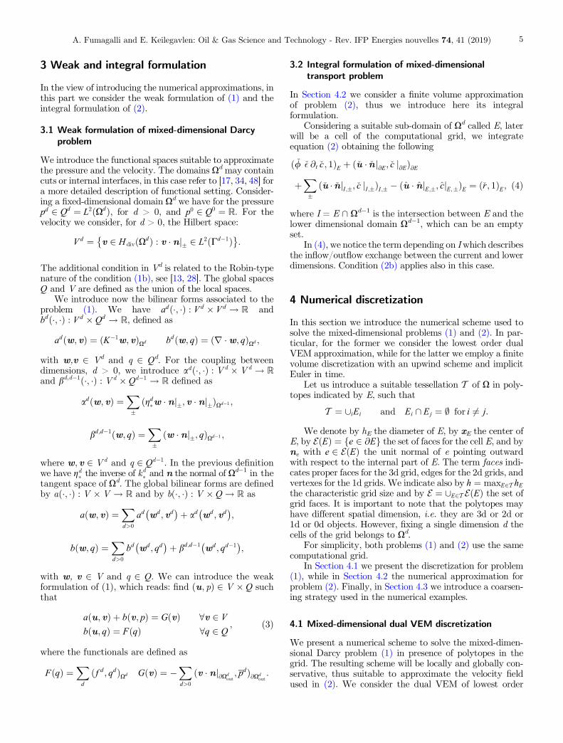
ð �/ �� @t �c; 1ÞE þ ð�u � �n j@E;�c j@EÞ@EþX�

ð�u � �njI;�;�c jI;�ÞI ;� � ðu � njE;�; cjE;�ÞE ¼ ð�r; 1ÞE; ð4Þ

where I = E \ Xd�1 is the intersection between E and thelower dimensional domain Xd�1, which can be an emptyset.

In (4), we notice the term depending on Iwhich describesthe inflow/outflow exchange between the current and lowerdimensions. Condition (2b) applies also in this case.

4 Numerical discretization

In this section we introduce the numerical scheme used tosolve the mixed-dimensional problems (1) and (2). In par-ticular, for the former we consider the lowest order dualVEM approximation, while for the latter we employ a finitevolume discretization with an upwind scheme and implicitEuler in time.

Let us introduce a suitable tessellation T of X in poly-topes indicated by E, such that

T ¼ [iEi and Ei \ Ej ¼ ; for i 6¼ j:

We denote by hE the diameter of E, by xE the center ofE, by EðEÞ ¼ e 2 @Ef g the set of faces for the cell E, and byne with e 2 EðEÞ the unit normal of e pointing outwardwith respect to the internal part of E. The term faces indi-cates proper faces for the 3d grid, edges for the 2d grids, andvertexes for the 1d grids. We indicate also by h ¼ maxE2T hEthe characteristic grid size and by E ¼ [E2T EðEÞ the set ofgrid faces. It is important to note that the polytopes mayhave different spatial dimension, i.e. they are 3d or 2d or1d or 0d objects. However, fixing a single dimension d thecells of the grid belongs to Xd.

For simplicity, both problems (1) and (2) use the samecomputational grid.

In Section 4.1 we present the discretization for problem(1), while in Section 4.2 the numerical approximation forproblem (2). Finally, in Section 4.3 we introduce a coarsen-ing strategy used in the numerical examples.

4.1 Mixed-dimensional dual VEM discretization

We present a numerical scheme to solve the mixed-dimen-sional Darcy problem (1) in presence of polytopes in thegrid. The resulting scheme will be locally and globally con-servative, thus suitable to approximate the velocity fieldused in (2). We consider the dual VEM of lowest order

A. Fumagalli and E. Keilegavlen: Oil & Gas Science and Technology - Rev. IFP Energies nouvelles 74, 41 (2019) 5

degree, for more details on the derivation and on the anal-ysis of the method, see [26–33].

4.1.1 Discrete function spaces

We introduce finite dimensional spaces to approximate theDarcy velocity u and the pressure p in each element of thegrid. For simplicity we consider a single dimension and, ifnot essential, we drop the superscript d to simplify notation.Again, the differential operators are understood to bedefined on the tangential space. Given an element E thelocal discretization space for the pressure is Qd

hðEÞ ¼P0ðEÞ � L2ðEÞ, where PrðEÞ is the space of polynomial oforder r on the domain E. While higher-order dual VEMapproximations are possible, see [31, 32], the solution willoften have low regularity caused by fractures or generalpermeability heterogeneities. We therefore stay with thelowest order formulation, as is common practice in the field.For the velocity we need to introduce the following space:

V dhðEÞ ¼ v 2 HdivðEÞ : v � ne 2 P0ðeÞ8e 2 EðEÞ;f

r � v 2 P0 Eð Þ;r v ¼ 0g:The shape of the functions in V d

hðEÞ is not defined a-prioriand is implicitly defined by V d

hðEÞ. The curl-free condition isnecessary to uniquely define the elements in V d

hðEÞ. Weindicate by V d

h the velocity approximation space in thesame dimensional grid and by Vh the global discretizationspace for the velocity formed by the compoundðV 1

h; :::; VNh Þ. Similarly, Qd

h indicates the pressure approxi-mation space in the same dimension d while Qh is the globaldiscretization space. For the velocity, we impose to the faceswhich are not in contact with different dimensions to be sin-gle value. Otherwise, the degree of freedom is doubled andconnected thorough the coupling condition (1b) to thelower dimensional object. See Figure 3 for an example.

4.1.2 Approximation of bilinear forms

With the previous definition of Qh and Vh it is immediate toapproximate the bilinear form b for all the dimensions as wellas the bilinear forms associatedwith the coupling conditions,ad and bd,d�1. The functionals F and G are discretizedsimilarly. The bilinear forms ad are not immediately com-putable with the degrees of freedom introduced, but requirethe definition of a suitable projection operator. First, weintroduce the local space

VdhðEÞ ¼ v 2 V d

h Eð Þ : v ¼ Krv; for a v 2 P1ðEÞ� �

; ð5Þ

and the projection operator is defined asP0 : Vd

hðEÞ ! VdhðEÞ such that given v 2 Vd

hðEÞ we haveadðv �P0v;wÞ ¼ 0 for all w 2 Vd

hðEÞ. Note that the spaceP1ðEÞ in the definition of Vd

hðEÞ will be approximated by a(tangential) monomial basis. Where we are assuming aconstant value of the permeability in the element E. For(5) to make sense, the permeability must be constant ineach cell. As discussed above, the permeability will inpractice often be spatially varying on all scales due tothe presence of smaller scale heterogeneities. Inclusion ofspatially varying permeabilities within a computational

cell would require corresponding modifications of theapproximation order for pressure and flux. Our preferredapproach to including more permeability variations is tostay with lowest order approximations, but instead refinethe grid.

With the orthogonality property it is possible to splitthe bilinear form ad in a term on Vd

hðEÞ and one on thead-orthogonal space of Vd

hðEÞ, namely

ad u; vð Þ ¼ ad P0u;P0vð Þ þ ad T 0u; T 0vð Þ¼ ðKru;rvÞXd þ adðT 0u; T 0vÞ

;

with T0 = I�P0. The first bilinear form is now fully com-putable with the velocity degrees of freedom introducedbefore and represents a consistency term with respect toad(u,v). The second term is not yet computable and canbe replaced by a stabilization term. Following the ideaspresented in [31–33], we approximate the term by,

ad T 0u; T 0vð Þ � 1sd T 0u; T 0vð Þ;where sd : Vd

hðEÞ VdhðEÞ ! R is the bilinear form asso-

ciated with the stabilization and 1 ¼ 1ðdÞ 2 Rþ is a scal-ing parameter described in the sequel. In details,denoting by u an element of the basis for Vd

hðEÞ, in ourcase we consider

sd T 0ux; T 0uhð Þ ¼XNdof

i¼1

dof i T 0uxð Þdof i T 0uhð Þ;

with Ndof the total number of velocity degrees of freedomof the element E and dof i : Vd

hðEÞ ! R is defined as

dof i uxð Þ ¼ ith degree of freedomof ux ¼ dix:

We introduce the discrete version adh : VdhðEÞ V d

hðEÞ ! Rof the bilinear form ad, defined as

adhðu; vÞ ¼ adðP0u;P0vÞ þ 1sdðT 0u; T 0vÞ;and the discrete version of the weak problem (3), whichreads: find ðu; pÞ 2 Vh Qh such that

ahðu; vÞ þ bðv; pÞ ¼ GðvÞ 8v 2 V h

bðu; qÞ ¼ F ðqÞ 8q 2 Qh

; ð6Þ

Fig. 3. Representation of the degrees of freedom for a 2d and 1dgrid. The pressure dof are represented by circles, red for the 2dgrid and green for the 1d. The velocity dof are depicted by yellowdiamonds for the 2d grid and purple diamonds for the 1d. Thenodes of the 2d grid are moved only for visualization purpose.

A. Fumagalli and E. Keilegavlen: Oil & Gas Science and Technology - Rev. IFP Energies nouvelles 74, 41 (2019)6

where ahðu; vÞ ¼P

d>0adhðud ; vdÞ þ adðwd ; vdÞ. The con-

struction of the discrete problem in term of local matrixcomputations is described in [28, 30].

The stabilization parameter 1 is used to impose thescaling on h of the stabilization term equivalent to theconsistency term. In practice we require that, for a fixeddimension d, there exists i�; i� 2 Rþ, independent fromthe discretization, such that

i�ad v; vð Þ � 1sd v; vð Þ � i�ad v; vð Þ 8 v 2 V dh :

Following [28], by a scaling computation we evaluatethe dependency of 1 from the local grid size hE and obtainthe following relation for a fix dimension d

1ðEÞ ¼ h2�dE :

Note that this expression is local and independent from themaximal dimension N of the problem.

4.1.3 Matrix formulation

We introduce the matrix formulation associated with theproblem (6). Considering the following matrices:

Ad½ �ij ¼ adh uj;ui

� �þ ad uj;ui

� �;

Bd½ �ij ¼ bd uj;wi

� �; Cd ;d�1½ �ij ¼ bd;d�1 uj;wi

� �;

and vectors

Gd½ �i ¼ GðuiÞ; F d½ �i ¼ F wið Þ;where / are basis for the pressure and �½ �i;j indicates theelement (i, j) in the matrix, a similar notation is usedfor vectors. The global problem reads for N = 3, solvethe following linear system

A3 B3 0 C3;2 0 0 0 0

BT3 0 0 0 0 0 0 0

0 0 A2 B2 0 C2;1 0 0

CT3;2 0 BT

2 0 0 0 0 0

0 0 0 0 A1 B1 0 C1;0

0 0 CT2;1 0 BT

1 0 0 0

0 0 0 0 0 0 I 0

0 0 0 0 CT1;0 0 0 0

266666666666664

377777777777775

u3

p3u2

p2u1

p1u0

p0

266666666666664

377777777777775¼

G3

F 3

G2

F 2

G1

F 1

0

0

266666666666664

377777777777775;

where ud and pd represent the vectors associated with thedegrees of freedom of velocity and pressure in each dimen-sion d. We note that the u0 is considered only for clearnessand to preserve the structure of the matrix. In practice, itis possible to remove u0 from the system.

4.2 Mixed-dimensional FV discretization

We consider now the discretization of equation (4). Forsimplicity, we consider a fixed time step Dt such thatT/Dt is an integer number. An implicit Euler is applied intime obtaining the semi-discrete version of (4)

ð �/ ��ð�c nþ1 � �c nÞ; 1ÞE�t

þ ��u � �n��

@E;�c nþ1

��@E

�@E

þX�

�u � �n��

I ;�;�cnþ1

��I ;�

I ;�

� u � n��E;�; c

nþ1��E;�

E

¼ ð�r nþ1; 1ÞE;where the superscript indicates the time step index,and c0 ¼ c. The approximation of the boundary integralsin the previous equation rely on an upwind scheme.We introduce a Kronecker-type delta as

du�n ¼ 1 if u � n 0

0 else

�:

Given a cell face e 2 EðEÞ we have

�u � �n je;�c nþ1je�e

¼ �u � �n je d�u � �n je�c

nþ1ðEÞ þ ð1� d�u � �n jeÞ�c nþ1ðLÞ�;�where the cells K and L share the face e. Given a cell Esuch that one of its faces, e, intersects one side of I, we get

u � nje; cnþ1je� �

e

¼ u � nje du�nje cnþ1 Eð Þ þ 1� du�nje

� ��cnþ1 �eÞð �;�

where �e indicates a cell in the co-dimensional grid which isin communication with the face e. Finally, on side givingan element E of the last term of the semi-discrete problemcan be approximated by

u � njE; cnþ1jE� �

E

¼ u � njE du�nje cnþ1ðEÞ þ ð1� du�njeÞ�c nþ1ðEÞ�;�

where E represents the cell in the higher dimensional gridwhich has a face e in communication with the cell E.The previous condition applies to both the equi- andco-dimensional coupling, see Figure 4 for an example.Note that the chosen discretization is compatible withthe coupling condition (2b).

For the matrix formulation of the transport problem, weintroduce the following matrices

Md½ �ii ¼ð/d�d ; 1Þi

�t; Ud½ �ii ¼

Xj2N ðiÞ;e2i\j

ðud � nd je; dud �nd jeÞe;

Ud½ �ij ¼X

j2N ið Þ;e2i\jðud � nd je; 1� dud �nd jeÞe;

whereN ðEÞ is the set of all neighbor cells of E, i and j indi-cate generic cells and e is a face shared by i and j. For thecoupling between dimensions we have

Ud;d�1½ �ii ¼X

j2N d�1 ið Þðud � nd jj; dud �nd jjÞj;

A. Fumagalli and E. Keilegavlen: Oil & Gas Science and Technology - Rev. IFP Energies nouvelles 74, 41 (2019) 7

Ud;d�1½ �ij ¼X

j2N d�1 ið Þðud � nd jj; 1� dud �nd jjÞj;

where Nd�1ðEÞ is the set of all neighbor cells of E in the

lower-dimensional grid. We obtain also

Ud;dþ1½ �ii ¼ �X

j2N dþ1 ið Þðudþ1 � ndþ1ji; dudþ1�ndþ1jiÞi;

Ud;dþ1½ �ij ¼ �X

j2N dþ1ðiÞðudþ1 � ndþ1ji; 1� dudþ1�ndþ1jiÞi;

where Ndþ1ðEÞ is the set of all neighbor cells of E in the

higher-dimensional grid. We finally obtain the followinglinear system to be inverted

U 3 þM3 U 3;2 0 0

U 2;3 U 2 þM2 U 2;1 0

0 U 1;2 U 1 þM1 U 1;0

0 0 U 0;1 0

2666437775

cnþ13

cnþ12

cnþ11

cnþ10

2666437775 ¼

fn;nþ13

fn;nþ12

fn;nþ11

0

2666437775;

where cd represents the vector associated with the degreesof freedoms of the concentration in each dimension d. Inthe previous linear system fd represents the right-handside, formed as a combination of the source term rnþ1

dand the concentration at the previous time step. We get

fn;nþ1d ¼ Mdcnd þ rnþ1

d :

4.3 Coarsening strategy

The construction of conforming grids in the presence of sev-eral fractures can be a challenging task, especially in 3d. Inthis work, our grids are constructed by the Gmsh mesh gen-erator [49]. In the presence of almost intersecting fracturesor small fracture branches, the grid may contain a highnumber of simplex cells, resulting in a high computational

cost. To overcome this difficulty, we exploit the ability ofVEM to handle cells of arbitrary geometry. To be specific,the theory developed in [30–33] requires star-shaped cells,however the study carry out in [50] shows that the VEMis able to handle also cells with cuts.

Motivated by these observations we introduce a coars-ening scheme that merges small simplex cells into largerpolygons or polyhedra. Starting from a given simplex grid,the algorithm computes the measure (area or volume) of thecells. Given the cell c with the smallest measure, it will bemerged to one or more neighboring cells, based on theirrespective measure, creating a new coarse cell. The cluster-ing stops when a cell measure threshold is reached. The cellsused in discretization are thus general polytopes, formed asunions of simplexes.

The algorithm does not guarantee any regularity of thefinal grid, as illustrated in Figure 5.

We emphasize that as elements are aggregated, a newelement with many faces is generated. The local matriceswill be denser and larger comparing to the original gridand increase the stencil of the global matrix. Nevertheless,the coarsening algorithm will decrease the computationalcost. Other strategies are possible but not considered in thiswork.

Finally, we note that the assumption of a cell-wise con-stant permeability applies also in this case. Thus, mergingof cells with different permeabilities requires the computa-tion of an average permeability. Correspondingly, for highlyheterogeneous media, it may be beneficial to consider alsocell permeability as a parameter in the coarsening algorithm.

5 Applicative examples

We present three examples and test cases to assess the pre-sented models and numerical schemes. The first example,presented in Section 5.1, considers an extensive validationof the mixed-dimensional Darcy problem solved by VEMthrough a benchmark study presented in [51]. The secondtest case, in Section 5.2, considers the transport problemand analyzes the impact of the coarsening strategy on theresults. Finally, in Section 5.3 a realistic 3d example is intro-duced and studied. In all the forthcoming examples weassume unitary porosity and zero source terms for theconcentration and Darcy equations. The other parameterswill be specified.

(a) (b) (c)

Fig. 4. Representation of the coupling between dimension for the upwind discretization scheme. (a) Between two cells in the samedimension d. (b) Between a d-dimensional cell and a d � 1-dimensional cell. (c) Between a d + 1-dimensional cell and a d-dimensionalcell.

A. Fumagalli and E. Keilegavlen: Oil & Gas Science and Technology - Rev. IFP Energies nouvelles 74, 41 (2019)8

In all of the forthcoming examples a “Blue to RedRainbow’’ color map is used.

The examples are part of the PorePy package, which isa simulation tool for fractured and deformable porousmedia written in Python. See [52] and github.com/pmgber-gen/porepy for more details.

5.1 Benchmark comparison

To validate the presentedmodel, we consider the benchmarkstudy presented in [51], specifically cases 1 and 4. The refer-ence solutions pref were computed with a mimetic finite dif-ference method [53] on a very fine grid that is able torepresent the thickness of the fractures by considering theclassical Darcy model. The error is thus evaluated by

err2 ¼ffiffiffiffiffiffiffiffiffiffiffiffiffiffiffiffiffiffiffiffiffiffiffiffiffiffiffiffiffiffiffiffiffiffiffiffiffiffiffiffiffiffiffiffiffiffiffiffiffiffiffiffiffiffiffiffiffiffiffiffiffiffiffiffiffiffiffiffiffiffiffiffiffi

1

jX2j�ref

XE¼Eref\E2

jEj p2jE2 � pref jErefð Þ2s

;

err1 ¼ffiffiffiffiffiffiffiffiffiffiffiffiffiffiffiffiffiffiffiffiffiffiffiffiffiffiffiffiffiffiffiffiffiffiffiffiffiffiffiffiffiffiffiffiffiffiffiffiffiffiffiffiffiffiffiffiffiffiffiffiffiffiffiffiffiffiffiffiffiffiffiffiffi

1

jX1j�ref

XE¼Eref\E1

jEj p1jE1 � pref jErefð Þ2s

;

for the matrix err2 and for the fractures err1, where�ref ¼ ðmax pref �min prefÞ2 and E2 is a cell in themixed-dimensional problem related to the rock matrix,respectively E1 for the fracture. The errors are computedon the reference grid, p1 is assumed constant on thenormal direction of the fracture in the equi-dimensionalsetting.

For more detail of problem setting refer to the aforemen-tioned work.

5.1.1 Benchmark 1: regular fracture network

The problem is inspired by Geiger et al. [54] with differentboundary conditions and material properties. The domainis the unit square containing six fractures, sketched inFigure 6. The matrix permeability is taken as unitary,and the fracture aperture is set equal to 10�4. No fluxboundary conditions are imposed on the top and bottomof the domain, while unitary pressure is imposed onthe right boundary and �1 as flux on the left boundary.

The source term is set to zero. We consider two possibilitiesfor fracture permeability: it is either highly conductive withpermeability 104 and has conductivity with permeability10�4. In the former case the solution obtained with themethod presented previously along with the computationalgrid are presented in Figure 7(a), the latter in (b). Weobserve a good agreement between the computed and refer-ence solutions, the latter is described in [51]. We point outthat some of the elements present in Figure 7 are notconvex.

To obtain a more detailed comparison we consider twoplots over line for the permeable case and one for the block-ing case, shown in Figure 8. From now on, the methodpresented in this paper is labeled as VEM. Also in this case,the agreement between the computed and referencesolutions is comparable to the other methods which are ableto represent blocking fractures. The small oscillations in theline plots are related to grid effects.

Finally, in both cases we consider the error decay forboth the rock matrix and the system of fractures. We con-sider a family of three grids where the coarsening is appliedin all the cases. We obtain again non-convex elements in allthe grids. Figure 9 plots for conductive and blocking frac-tures the error decay. The errors are comparable with thoseof others methods able to represent permeable and blockingfractures. In the latter case we note a stagnation of the

Fig. 6. Domain with fractures (in red) and fracture intersec-tions (in blue) for problem in Section 5.1.1.

(a) (b)

Fig. 5. Example of the coarsening strategy adopted. (a) The computational grid is artificially forced to be finer at the tip of afracture. (b) The resulting grid after the coarsening. Clearly the cell measures are comparable.

A. Fumagalli and E. Keilegavlen: Oil & Gas Science and Technology - Rev. IFP Energies nouvelles 74, 41 (2019) 9

fracture error which bounds the order of converge. Thisphenomenon is common also for other methods presentedin the benchmark study [51].

5.1.2 Benchmark 4: a realistic case

We consider now a complex system of 64 fractures from areal outcrop. The domain is X = (0, 700 m) (0, 600 m),

sketched in Figure 10.We consider constant rock permeabil-ity equal to 10�14 m2, uniform fracture permeability10�8 m2, and fracture aperture 10�2 m2. We impose a pres-sure gradient at the boundary from the left (1 013 250 Pa)to the right (0 Pa), and no flow condition on the top andbottom of the domain. The source term is set to zero. Alsoin this case, a triangular grid is coarsened to reduce the gridcomplexity. The reference grid is composed by 12 472 2d

(a) (b) (c)

Fig. 7. Benchmark 1. (a) Pressure solution (range (1, 1.6)) with conductive fractures and computational grid. (b) Pressure solution(range (1, 3.6)) with blocking fractures and computational grid. (c) Zoom of the grid used.

(a) (b) (c)

Fig. 8. Benchmark 1 with conductive fractures. (a) Pressure along horizontal line at y = 0.7 with permeable fracture. (b) Pressurealong vertical fracture at x = 0.5 with permeable fractures. (c) Pressure along the line (0.0, 0.1)–(0.9, 1.0) with blocking fractures.

Fig. 9. Benchmark 1, error evolution for the matrix and the fractures with conductive and blocking fractures.

A. Fumagalli and E. Keilegavlen: Oil & Gas Science and Technology - Rev. IFP Energies nouvelles 74, 41 (2019)10

cells, 1317 1d cells, and 85 0d cells. The coarse algorithmdecreases the number of 2d cells down to 4703. The totalnumber of degrees of freedom is 19 075 for the coarsegrid.

The computed solution is represented in Figure 12(a),which matches the solution of the others method consideredin [51]. Because of the complexity of the network, conform-ing and non-matching methods may pose a constraint tothe grid generation in particular for close fractures. How-ever, the method presented allows general grid cells, andthus alleviate the computational cost for the simulation.For an illustration of the computational grid, we refer toFigure 11, which zooms in on a region with almost intersect-ing fractures.

As shown in Figure 11, some of the grid cells are non star-shaped or even contains cuts. For a more detailed discussionrefer to [50]. Finally, to validate in more detail the computedsolution we present two plots over line and compare them

with the solutions obtained in the benchmark study, seeFigure 12. The curves for the current method are in goodagreement with the others. Again, the small oscillations thatcan be observed are related to grids effects.

5.2 Passive scalar transport

In this part we consider both mixed-dimensional models (1)and (2) to simulate a passive scalar transport. We considerthe geometry presented in Section 5.1.2 and compare thesolution obtained with both grids in Figure 11 for perme-able and blocking fractures. For the reference grid, the totalnumber of degrees of freedom is 35 578. The aim of this testis to validate the quality of the Darcy velocity on thepassive scalar in presence of the grid coarsening. In the fol-lowing fracture aperture is constant and equal to 10�2 m, apressure gradient from the right to left boundary of thedomain of 3 107 Pa, a final simulation time of 40 years.

5.2.1 Permeable fractures

We consider highly permeable fractures with tangential per-meability of 5 10�6 m2 and normal permeability of2.5 10�9 m2. The matrix permeability is set to 2.5 10�11 m2. Figure 13 compares the solutions obtained onthe reference triangular grid and on the coarse grid. More-over Figure 14(a) presents a comparison of the passive sca-lar production. We notice the good agreement in both thepressure and concentration fields as well as in the produc-tion curve. We can conclude that in this case the grid coars-ening is not affecting the quality of the computed solutions.

Finally, in Figure 14(b) the temporal error decay isreported. The spatial discretization is fixed and we considera sequence of simulation with (10, 20, 40, 80, 160, 320, 640,

(a)

(b)

Fig. 11. Benchmark 4. (a) Original grid composed by 12 302 2d-cells and 35 153 VEM dof and coarsened grid composed by4599 2d-cells and 18 803 VEM dof. (b) A zoom on almost intersecting fractures for the original and coarsened grids, respectively. Thezoom is referred to the small rectangle at position, approximately (360, 350).

Fig. 10. Domain with fractures (in red) for problem inSection 5.1.2.

A. Fumagalli and E. Keilegavlen: Oil & Gas Science and Technology - Rev. IFP Energies nouvelles 74, 41 (2019) 11

1280, 2560, 5120) time steps each. The error is computed asthe L2 difference from a reference solution obtained with 105

time steps after 10 years. A unitary error decay is achieved,coherent with the numerical scheme considered.

5.2.2 Blocking fractures

Next, we consider blocking fractures with tangential andnormal permeability of 7.5 10�16 m2. Matrix permeabilityis set to 7.5 10�11 m2. Figure 15 compares the solutionsobtained on the reference triangular grid and on the coarse

grid. In this case we notice a pickpeak of velocity in the ref-erence case due to small elements close to almost intersect-ing fractures. This may affect an explicit in time solver.Figure 16(a) presents a comparison of the passive scalarproduction. We notice the good agreement in both the pres-sure and concentration fields as well as in the production.We can conclude that also in this case the grid coarseningis not affecting the quality of the computed solutions.

Again, the temporal error decay is reported, seeFigure 16(b). The spatial discretization is fixed and weassign (10, 20, 40, 80, 160, 320, 640, 1280, 2560, 5120) time

(a)

(b)

Fig. 13. Permeable fractures. (a) Reference and coarse solutions for pressure and velocity, as arrows. (b) Reference and coarsesolutions for concentration of the passive scalar.

(a) (b) (c)

Fig. 12. Benchmark 4. (a) Pressure solution computed with VEM. The pressure ranges in [0, 1 013 250] Pa. (b) Pressure alonghorizontal line at y = 500 m. (c) Pressure along vertical line at x = 625 m.

A. Fumagalli and E. Keilegavlen: Oil & Gas Science and Technology - Rev. IFP Energies nouvelles 74, 41 (2019)12

steps, respectively. A unitary error decay is achieved, con-sistent with the numerical scheme considered.

5.3 Passive scalar transport on a realistic 3d-network

In this examplewe consider a realistic geometry for a geother-mal system. We study a partial reconstruction of fracturesfrom test site at Soultz-sous-Forêts in France, for moredetails see [55]. The network is composed by 20 fractures

represented as polygons with 10 edges each. The fractureintersections result in 33 1d objects and 4 0d objects. In thiscase the full model is needed to accurately simulate the fluidflow and transport on the domain. The fracture geometry isrepresented in Figure 17.We assume rock matrix permeabil-ity as 7.5 10�10 m2 and fracture permeability, in both thenormal and tangential direction, equal to 5 10�5 m2. Thefracture aperture is �2 = 10�2 m and, for the lower dimen-sional objects, we consider their “aperture’’ as the square

(a) (b)

Fig. 14. Permeable fractures. (a) Comparison of passive scalar production at the outflow between the reference triangular grid andthe coarse grid. (b) Temporal error decay with reference Oð�tÞ in black.

(a)

(b)

Fig. 15. Blocking fractures. (a) Reference and coarse solutions for pressure and velocity, as arrows. (b) Reference and coarse solutionsfor concentration of the passive scalar.

A. Fumagalli and E. Keilegavlen: Oil & Gas Science and Technology - Rev. IFP Energies nouvelles 74, 41 (2019) 13

and the cube of the fracture aperture, respectively for the 1dand 0d objects. We impose a pressure from the top tobottom of the domain and no flux boundary conditionson the other sides. The reference grid is composed by44 331 tetrahedra, 6197 triangles for the 2d grids, 151 seg-ments for the 1d grids, and 4 point-cells for the 0d grids.After the coarsening algorithm the resulting grid iscomposed by 16 108 polyhedra, and for the lower dimen-sional objects the grids are untouched. See Figure 19(b)for an example of coarse cells. The transport simulationruns for 40 years and, for the implicit Euler scheme, we con-sider 100 time steps.

The objective is to study the robustness of the virtualelements associated with the coarsening strategy and detectif the coarse model gives accurately enough results. Thepressure solution and the concentration of the scalar passiveare depicted in Figures 17 and 18, respectively, for both thereference and coarse case. Both the pressure and concentra-tion profiles for the two grids are in good agreement. Toanalyze the macroscopic behavior of the resulting solution

(a) (b)

Fig. 16. Blocking fractures. (a) Comparison of passive scalar production at the outflow between the reference triangular grid and thecoarse grid. (b) Temporal error decay with reference Oð�tÞ in black.

Fig. 17. On the left representation of the 20 fractures coloredby their identification number. Pressure and velocity for boththe reference and coarse grids. The pressure is scaled between 0and 4.8 107 Pa.

Fig. 18. (a) Three time steps on the reference grid for the concentration. (b) At the same steps, the concentration computed on thecoarse grid.

A. Fumagalli and E. Keilegavlen: Oil & Gas Science and Technology - Rev. IFP Energies nouvelles 74, 41 (2019)14

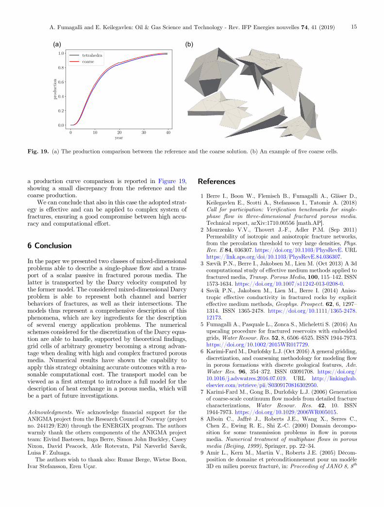
a production curve comparison is reported in Figure 19,showing a small discrepancy from the reference and thecoarse production.

We can conclude that also in this case the adopted strat-egy is effective and can be applied to complex system offractures, ensuring a good compromise between high accu-racy and computational effort.

6 Conclusion

In the paper we presented two classes of mixed-dimensionalproblems able to describe a single-phase flow and a trans-port of a scalar passive in fractured porous media. Thelatter is transported by the Darcy velocity computed bythe former model. The considered mixed-dimensional Darcyproblem is able to represent both channel and barrierbehaviors of fractures, as well as their intersections. Themodels thus represent a comprehensive description of thisphenomena, which are key ingredients for the descriptionof several energy application problems. The numericalschemes considered for the discretization of the Darcy equa-tion are able to handle, supported by theoretical findings,grid cells of arbitrary geometry becoming a strong advan-tage when dealing with high and complex fractured porousmedia. Numerical results have shown the capability toapply this strategy obtaining accurate outcomes with a rea-sonable computational cost. The transport model can beviewed as a first attempt to introduce a full model for thedescription of heat exchange in a porous media, which willbe a part of future investigations.

Acknowledgments. We acknowledge financial support for theANIGMA project from the Research Council of Norway (projectno. 244129/E20) through the ENERGIX program. The authorswarmly thank the others components of the ANIGMA projectteam: Eivind Bastesen, Inga Berre, Simon John Buckley, CaseyNixon, David Peacock, Atle Rotevatn, Pål Næverlid Sævik,Luisa F. Zuluaga.

The authors wish to thank also: Runar Berge, Wietse Boon,Ivar Stefansson, Eren Uçar.

References

1 Berre I., Boon W., Flemisch B., Fumagalli A., Gläser D.,Keilegavlen E., Scotti A., Stefansson I., Tatomir A. (2018)Call for participation: Verification benchmarks for single-phase flow in three-dimensional fractured porous media.Technical report, arXiv:1710.00556 [math.AP].

2 Mourzenko V.V., Thovert J.-F., Adler P.M. (Sep 2011)Permeability of isotropic and anisotropic fracture networks,from the percolation threshold to very large densities, Phys.Rev. E 84, 036307. https://doi.org/10.1103/PhysRevE. URLhttps://link.aps.org/doi/10.1103/PhysRevE.84.036307.

3 Sævik P.N., Berre I., Jakobsen M., Lien M. (Oct 2013) A 3dcomputational study of effective medium methods applied tofractured media, Transp. Porous Media, 100, 115–142. ISSN1573-1634. https://doi.org/10.1007/s11242-013-0208-0.

4 Ssvik P.N., Jakobsen M., Lien M., Berre I. (2014) Aniso-tropic effective conductivity in fractured rocks by expliciteffective medium methods, Geophys. Prospect. 62, 6, 1297–1314. ISSN 1365-2478. https://doi.org/10.1111/1365-2478.12173.

5 Fumagalli A., Pasquale L., Zonca S., Micheletti S. (2016) Anupscaling procedure for fractured reservoirs with embeddedgrids,Water Resour. Res. 52, 8, 6506–6525. ISSN 1944-7973.https://doi.org/10.1002/2015WR017729.

6 Karimi-FardM., Durlofsky L.J. (Oct 2016) A general gridding,discretization, and coarsening methodology for modeling flowin porous formations with discrete geological features, Adv.Water Res. 96, 354–372. ISSN 03091708. https://doi.org/10.1016/j.advwatres.2016.07.019. URL http://linkinghub.elsevier.com/retrieve/pii/S0309170816302950.

7 Karimi-Fard M., Gong B., Durlofsky L.J. (2006) Generationof coarse-scale continuum flow models from detailed fracturecharacterizations, Water Resour. Res. 42, 10. ISSN1944-7973. https://doi.org/10.1029/2006WR005015.

8 Alboin C., Jaffré J., Roberts J.E., Wang X., Serres C.,Chen Z., Ewing R. E., Shi Z.-C. (2000) Domain decompo-sition for some transmission problems in flow in porousmedia. Numerical treatment of multiphase flows in porousmedia (Beijing, 1999), Springer, pp. 22–34.

9 Amir L., Kern M., Martin V., Roberts J.E. (2005) Décom-position de domaine et préconditionnement pour un modèle3D en milieu poreux fracturé, in: Proceeding of JANO 8, 8th

(a) (b)

Fig. 19. (a) The production comparison between the reference and the coarse solution. (b) An example of five coarse cells.

A. Fumagalli and E. Keilegavlen: Oil & Gas Science and Technology - Rev. IFP Energies nouvelles 74, 41 (2019) 15

Conference on Numerical Analysis and Optimization,December 2005.

10 Boon W.M., Nordbotten J.M., Yotov I. (2018) Robustdiscretization of flow in fractured porous media, SIAM J.Numer. Anal. 56, 4, 2203–2233. https://doi.org/10.1137/17M1139102.

11 Faille I., Fumagalli A., Jaffré J., Roberts J.E. (2016) Modelreduction and discretization using hybrid finite volumes offlow in porous media containing faults, Comput. Geosci. 20,2, 317–339. ISSN 15731499. https://doi.org/10.1007/s10596-016-9558-3.

12 Knabner P., Roberts J.E. (2014) Mathematical analysis of adiscrete fracture model coupling Darcy flow in the matrixwith Darcy-Forchheimer flow in the fracture, ESAIM: Math.Model. Numer. Anal. 48, 1451–1472. ISSN 1290-3841.https://doi.org/10.1051/m2an/2014003. URL http://www.esaim-m2an.org/article_S0764583X1400003X.

13 Martin V., Jaffré J., Roberts J.E. (2005) Modeling fracturesand barriers as interfaces for flow in porous media, SIAM J.Sci. Comput. 26, 5, 1667–1691. ISSN 1064-8275. https://doi.org/10.1137/S1064827503429363. URL http://scitation.aip.org/getabs/servlet/GetabsServlet?prog=normal&id=SJ0CE3000026000005001667000001&idtype= cvips&gifs=yes.

14 Schwenck N., Flemisch B., Helmig R., Wohlmuth B.I. (2015)Dimensionally reduced flow models in fractured porousmedia: crossings and boundaries, Comput. Geosci. 19, 6,1219–1230. ISSN 1420-0597. https://doi.org/10.1007/s10596-015-9536-1.

15 Tunc X., Faille I., Gallouet T., Cacas M.C., Havé P. (2012)A model for conductive faults with non-matching grids,Comput. Geosci. 16, 277–296. ISSN 1420-0597. https://doi.org/10.1007/s10596-011-9267-x.

16 Angot P. (2003) A model of fracture for elliptic problems withflux and solution jumps, C. R. Math. 337, 6, 425–430. ISSN1631-073X. https://doi.org/10.1016/S1631-073X(03)00300-5.URL http://www.sciencedirect.com/science/article/pii/S1631073X03003005.

17 Angot P., Boyer F., Hubert F. (2009) Asymptotic andnumerical modelling of flows in fractured porous media,M2AN Math Model. Numer. Anal. 43, 2, 239–275. ISSN0764-583X. https://doi.org/10.1051/m2an/2008052.

18 Chave F.A., Di Pietro D., Formaggia L. (2017) A HybridHigh-Order method for Darcy flows in fractured porousmedia, Technical report, HAL archives, 2017. URL https://hal.archives-ouvertes.fr/hal-01482925.

19 Karimi-Fard M., Firoozabadi A. (2003) Numerical simula-tion of water injection in fractured media using the discrete-fracture model and the Galerkin method, SPE Reserv. Eval.Eng. 6, 02, 117–126.

20 Ahmed R., Edwards M.G., Lamine S., Huisman B.A.H., PalM. (2015) Control-volume distributed multi-point fluxapproximation coupled with a lower-dimensional fracturemodel, J. Comput. Phys. 284, 462–489. ISSN 0021-9991.https://doi.org/10.1016/jjcp.2014.12.047. http://www.sciencedirect.com/science/article/pii/S0021999114008705.

21 Brenner K., Hennicker J., Masson R., Samier P. (September2016) Gradient discretization of hybrid-dimensional Darcy flowin fractured porous media with discontinuous pressures atmatrix-fracture interfaces, IMA J. Numer. Anal. https://doi.org/10.1093/imanum/drw044. URL https://hal.archives-ouvertes.fr/hal-01192740.

22 Brenner K., Hennicker J., Masson R., Samier P. (2018)Hybrid-dimensional modelling of two-phase flow through

fractured porous media with enhanced matrix fracturetransmission conditions, J. Comput. Phys. 357, 100–124.ISSN 0021-9991. https://doi.org/10.1016/j.jcp.2017.12.003.http://www.sciencedirect.com/science/article/pii/S0021999117308781.

23 Brenner K., Groza M., Guichard C., Masson R. (2015)Vertex approximate gradient scheme for hybrid dimensionaltwo-phase Darcy flows in fractured porous media, ESAIM:Math. Model. Numer. Anal. 49, 2, 303–330. https://doi.org/10.1051/m2an/2014034.

24 Antonietti P.F., Formaggia L., Scotti A., Verani M., VerzottiN. (2016) Mimetic finite difference approximation of flows infractured porous media, ESAIM: M2AN 50, 3, 809–832.https://doi.org/10.1051/m2an/2015087.

25 Scotti A., Formaggia L., Sottocasa F. (2017) Analysis of amimetic finite difference approximation of flows in fracturedporous media, ESAIM: M2AN. https://doi.org/10.1051/m2an/2017028.

26 Benedetto M.F., Berrone S., Pieraccini S., Scialò S. (2014) Thevirtual element method for discrete fracture network simula-tions, Comput. Methods Appl. Mech. Eng. 280, 0, 135–156.ISSN 0045-7825. https://doi.org/10.1016/j.cma.2014.07.016.

27 Benedetto M.F., Berrone S., Borio A., Pieraccini S., Scialò S.(2016) A hybrid mortar virtual element method for discretefracture network simulations, J. Comput. Phys. 306,148–166. ISSN 0021-9991. https://doi.org/10.1016/jjcp.2015.11.034. http://www.sciencedirect.com/science/article/pii/S0021999115007743.

28 Fumagalli A., Keilegavlen E. (2018) Dual virtual elementmethod for discrete fractures networks, SIAM J. Sci.Comput. 40, 1, B228–B258. https://doi.org/10.1137/16M1098231.

29 da Veiga L.B., Brezzi F., Cangiani A., Manzini G.,Marini L.D., Russo A. (2013) Basic principles of virtualelement methods, Math. Models Methods Appl. Sci. 23, 01,199–214. https://doi.org/10.1142/S0218202512500492.

30 da Veiga L.B., Brezzi F., Marini L.D., Russo A. (2014) Thehitchhiker’s guide to the virtual element method, Math.Models Methods Appl. Sci. 24, 08, 1541–1573. https://doi.org/10.1142/S021820251440003X.

31 da Veiga L.B., Brezzi F., Marini L.D., Russo A. (Jun 2014) H(div) and H(curl)-conforming VEM, Numer. Math. 133, 2,303–332. ISSN 0945-3245. https://doi.org/10.1007/s00211-015-0746-1.

32 da Veiga L.B., Brezzi F., Marini L.D., Russo A. (2016) Mixedvirtual element methods for general second order ellipticproblems on polygonal meshes, ESAIM: M2AN 50, 3,727–747. https://doi.org/10.1051/m2an/2015067.

33 Brezzi F., Falk R.S., Marini D.L. (2014) Basic principles ofmixed virtual element methods, ESAIM: M2AN 48,1227–1240. https://doi.org/10.1051/m2an/2013138.

34 Frih N., Martin V., Roberts J.E., Saâda A. (2012) Modelingfractures as interfaces with nonmatching grids, Comput.Geosci. 16, 4, 1043–1060. ISSN 1420-0597. https://doi.org/10.1007/s10596-012-9302-6.

35 Nordbotten J.M., Boon W., Fumagalli A., Keilegavlen E.(2018) Unified approach to discretization of flow in fracturedporous media, Comput. Geosci. ISSN 1573-1499. https://doi.org/10.1007/s10596-018-9778-9.

36 Berrone S., Pieraccini S., Scialò S. (2013) On simulations ofdiscrete fracture network flows with an optimization-basedextended finite element method, SIAM J. Sci. Comput. 35, 2,908–935. https://doi.org/10.1137/120882883.

A. Fumagalli and E. Keilegavlen: Oil & Gas Science and Technology - Rev. IFP Energies nouvelles 74, 41 (2019)16

37 D’Angelo C., Scotti A. (2012) A mixed finite element methodfor Darcy flow in fractured porous media with nonmatchinggrids, Math. Model. Numer. Anal. 46, 02, 465–489.https://doi.org/10.1051/m2an/2011148.

38 Del Pra M., Fumagalli A., Scotti A. (2017) Well posedness offully coupled fracture/bulk Darcy flow with XFEM, SIAM J.Numer. Anal. 55, 2, 785–811. https://doi.org/10.1137/15M1022574.

39 Fumagalli A., Scotti A. (2013) A numerical method for two-phase flow in fractured porous media with non-matchinggrids, Adv. Water Res. 62, Part C(0), 454–464. ISSN0309-1708. https://doi.org/10.1016/j.advwatres.2013.04.001.URL https://www.sciencedirect.com/science/article/pii/S0309170813000523. Computational Methods in GeologicCO2 Sequestration.

40 Fumagalli A., Scotti A. (April 2014) An efficient XFEMapproximation of Darcy flows in arbitrarily fractured porousmedia, Oil Gas Sci. Technol. - Rev. IFP Energies nouvelles69, 4, 555–564. https://doi.org/10.2516/ogst/2013192. URLhttps://ogst.ifpenergiesnouvelles.fr/articles/ogst/abs/2014/04/ogst130007/ogst130007.html.

41 Tene M., Al Kobaisi M.S., Hajibeygi H. (2016) Multiscaleprojection-based embedded discrete fracture modelingapproach (f-ams-pedfm), ECMOR XIV-15th EuropeanConference on the Mathematics of Oil Recovery, August29–1 September 2016, Beurs van Berlage, EAGE.https://doi.org/10.3997/2214-4609.201601890.

42 Fumagalli A., Zonca S., Formaggia L. (July 2017) Advances incomputation of local problems for flow-based upscaling infractured reservoirs, Math. Comput. Simul. 137, 299–324.https://doi.org/10.1016/j.matcom.2017.01.007. URL https://www.sciencedirect.com/science/article/pii/S0378475417300320.

43 Li L., Lee S.H. (2008) Efficient field-scale simulation of blackoil in a naturally fractured reservoir through discrete fracturenetworks and homogenized media, SPE Reserv. Eval. Eng.11, 750–758. https://doi.org/10.2118/103901-PA.

44 Berrone S., Pieraccini S., Scialò S. (2013) A PDE-constrainedoptimization formulation for discrete fracture network flows,SIAM J. Sci. Comput., 35, 2, B487–B510. https://doi.org/10.1137/120865884.

45 Formaggia L., Fumagalli A., Scotti A., Ruffo P. (2014) Areduced model for Darcy’s problem in networks of fractures,ESAIM: Math. Model. Numer. Anal. 48, 1089–1116.https://doi.org/10.1051/m2an/2013132. URL https://www.esaim-m2an.org/articles/m2an/abs/2014/04/m2an130132/m2an130132.html.

46 Boon W.M., Nordbotten J.M., Vatne J.E. (2017) Mixeddi-mensional elliptic partial differential equations. Technicalreport, arXiv:1710.00556 [math.AP].

47 Fumagalli A., Scotti A. (2013) A reduced model for flow andtransport in fractured porous media with nonmatching grids,in: Cangiani A., Davidchack R.L., Georgoulis E., GorbanA.N., Levesley J., Tretyakov M.V. (eds), Numerical math-ematics and advanced applications 2011, Berlin, Heidelberg,Springer, pp. 499–507. ISBN 978-3-642-33133-6. https://doi.org/10.1007/978-3-642-33134-3_53.

48 Grisvard P. (1985) Elliptic problems in non-smooth domains,Vol. 24, Monographs and studies in mathematics, Pitman.

49 Geuzaine C., Remacle J.-F. (2009) Gmsh: A 3-d finite elementmesh generator with built-in pre- and post-processing facili-ties, Int. J. Numer. Methods Eng. 79, 11, 1309–1331. ISSN1097-0207. https://doi.org/10.1002/nme.2579.

50 Fumagalli A. (Dec. 2018) Dual virtual element method inpresence of an inclusion, Appl. Math. Lett. 86, 22–29.https://doi.org/10.1016/j.aml.2018.06.004. URL https://www.sciencedirect.com/science/article/pii/S0893965918301812.

51 Flemisch B., Berre I., Boon W., Fumagalli A., Schwenck N.,Scotti A., Stefansson I., Tatomir A. (January 2018) Bench-marks for single-phase flow in fractured porous media, Adv.Water Res. 111, 239–258. https://doi.org/10.1016/j.advwa-tres.2017.10.036. URL https://www.sciencedirect.com/science/article/pii/S0309170817300143.

52 Keilegavlen E., Fumagalli A., Berge R., Stefansson I., Berre I.(2017) Porepy: An open source simulation tool for flow andtransport in deformable fractured rocks. Technical report, arXiv:1712.00460 [cs.CE]. URL https://arxiv.org/abs/1712.00460.

53 Flemisch B., Rainer H. (2008) Numerical investigation of amimetic finite difference method, in: Finite volumes for complexapplications V – Problems and perspectives, Wiley–VCH,Germany, pp. 815–824.

54 Geiger S., Dentz M., Neuweiler I. (2011) A novel multi-ratedual-porosity model for improved simulation of fractured andmultiporosity reservoirs, SPE Reservoir Characterisationand Simulation Conference and Exhibition, 9–11 October,Abu Dhabi.

55 Sausse J., Dezayes C., Dorbath L., Genter A., Place J. (2010)3d model of fracture zones at soultzsous-for Sts based ongeological data, image logs, induced microseismicity andvertical seismic profiles, C. R. Geosci. 342, 7, 531–545.ISSN 1631-0713. doi: http://doi.org/10.1016/j.crte.2010.01.011. URL http://www.sciencedirect.com/science/article/pii/S1631071310000489.

A. Fumagalli and E. Keilegavlen: Oil & Gas Science and Technology - Rev. IFP Energies nouvelles 74, 41 (2019) 17