FSLTH-M-203 4

i Technical Report

Measurements of Tilt Anisoplanat-ismat the Firepond Facility

DTJ R. TGostf E LECTE .A ae

N • JAN 2 5 1983 R.N. Capes, Jr.J.J. Alves

I M.D. Zimmerman

"K AN. Roberts

4-;.

18 November 1988

Lincoln LaboratorN1ASSNICAIUSTTS I\IP•l .V OF TECIINOLOGY

Prepared f•r the Vcpartrmn•'nt o the Air For,:

1 i T1 I I VEri ri~ V: I)6 vorcm m,- (m)

PEPRODUCED FROMB EST AVAILABLE COPY

The work reported in this document was performed at Lincoln Laboratory, a(*,nter for research operated by Massachusetts Institute of Technology. Thiswork was sponsored by the Air Force Weapons Laboratory under Air ForceContract F19628-85-C-0002.

This report may be reproduced to satisfy needs of U.S. Government Agencies.

The views and conclusions contained in this document are those of thecontractor and should not be interpreted as necessarily representing the officialpolicies, either expressed or implied, of the United States Government.

This technical report has been reviewed and is approved for publication.

FOR THE COMMANDER

Hugh L. Southall, Lt. Col., USAFChief, ESD Lincoln Laboratory Project Office

Non-Lincoln Recipients

PLEASE DO NOT RETURN

Permission is given to destroy this documentwhen it is no longer needed.

MASSACHUSETTS INSTITUTE OF TECHNOLOGY

LINCOLN LABORATORY

MEASUREMENTS OF TILT ANISOPLANATISMAT THE FIREPOND FACILITY

R. TEOSTE.Md.D. ZIMMERMAN

Group 55

J.A. DALEY. JR. A.V, ROBERTSR.N. CAPES, JR. Group 76

J.J. ALVES

Group 52

ACce s.; ForTECHNICAL REPORT 815

F B-Ti T:,i •

18 NOVEMBER 1988 U.J -,

Approved for public release; distribution unlimited.

LEXINGTON MASSACHUSETTS

ABSTRACT

Tilt anisoplanatism is the atmosphere-induced differential tilt seen by a commontelescope observing two light sources separated by a very small angle. This reportsummarizes the results of tilt anisoplanatism measurements made at the FirepondFacility in Westford, Massachusetts. Two very precise visible quad trackers were usedto simultaneously track each component of selected binary stars whose angularseparations were in the range of 47 to 107 prad. While the report describes the trackinghardware and its characterization, the major contribution of this work is quantifyingthe tilt anisoplanatism under a variety of seeing conditions. The measurementsshowed that the magnitude of tilt anisoplanatism can be on the order of I-prad rms fora 1.2-m telescope, a value several times larger than previously believed. The frequencydistribution of the differential tilt is extremely variable, but most of the jitter strengthlies below 30 Hz, with almost negligible contributions above 100 Hz. Calculations ofthe tilt anisoplanatism magnitude were made by the Optical Sciences Company usingthe SLC and Hufnagel-Valley turbulence models. The calculations are in generalagreement with the measurements, but accurate predictions require precise atmo-spheric measurements as inputs to the models.

iii

TABLE OF CONTENTS

Abstract iiiList of Illustrations viiList of Tables ix

1. INTRODUCTION AND SUMMARY

1.1 Historical Background I1.2 Experimental Equipment 21.3 Summary of Results 3

2. EQUIPMENT DESCRIPTION 7

2.1 Firepond 1.2-m Telescope System 82.2 The Optical Tracker Package 92.3 The Fast Steering Mirror 122.4 Quad Tracker Electronics 132.5 Track-Data-Acquisition System 152.6 Stellar Scintillometer 17

3. SYSTEM PERFORMANCE 19

3.1 Tracker Noise Sources 193.2 Ultimate Bandwidth and Noise Floor Tests 203.3 Star Tracking Bandwidth Capabilities 233.4 Calibration of the Optical Error Signals 253.5 Angle-of-Arria! Calibration 253.6 Tracker Scale-r-..ctot Balance 26

4. TILT ANISOPLANATISM RESULTS 29

4.1 Description of an Observing Session 294.2 Double-Star Selection 304.3 Summary of Data Runs 314.4 Typical Processing of Results 33

4.4.1 Rotation of Data 344.4.2 Differential Tilt Power Spectral Densities 354.4.3 Determination of System Noise 374.4.4 Normal vs Flipped Differential Tilt 37

4.5 Monitoring of Atmospheric Variables 374.6 Tilt Anisoplanatism Data 42

4.6.1 Tilt Anisoplanatism vs Atmospheric Coherence Length 424.6.2 Tilt Anisoplanatism vs Isoplanatic Angle 43

4.7 Comparison of Firepond Data with Theory 47

4.7.1 Tilt Anisoplanatism vs Double-Star Separation 47

4.7.2 Tilt Anisoplanatism vs Normalized Separation 474.7.3 Longitudinal vs Lateral Component Magnitude 49

4.8 Power Spectral Density of the Differential Tilt 49

5. CONCLUS!ONS 57

ACKNOWLEDGMENTS 59

REFERENCES 61

vi

LIST OF ILLUSTRATIONS

FigureNo. Page

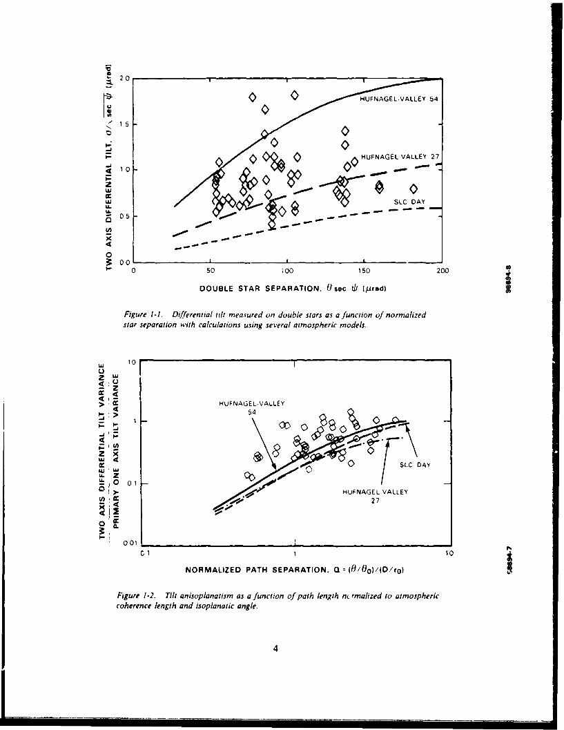
I-I Differential Tilt Measured on Double Stars as a Function ofNormalized Star Separation with Calculations Using SeveralAtmospheric Models 4

1-2 Tilt Anisoplanatism as a Function of Path Length Normalized toAtmospheric Coherence Length and lsolanatic Angle 4

2-1 Tilt Anisoplanatism Measurement Equipment 7

2-2 Firepond 1.2-m-Aperture Telescope with the 60-cm-ApertureFind%.r Telescope

2-3 Firepond 1.2-m-Aperture Telescope with the Binary Star TrackingEquipment Mounted on the Azimuth Axis 9

2-4 Optical Schematic of BinarN Star Tracker 10

2-5 Quad Detector with Four Photomultiplier Tubes I!

2-6 Quad Detector Pyramid and Circular Stop 12

2-7 Construction of the Fast Steering Mirror 13

2-8 Quad [racker Electronics 14

2-9 Data-Acquisition System 16

2-10 Twinkle Meter Schematic 18

3-1 Test Setup for Quad Trackers 20

3-2 Power Spectral Density of Fast Steering Mirror Position DuringHigh-Optical-Turbulence Tracking Tests 21

3-3 Power Spectral Density of Fast Steering Mirror Position DuringOptical Tests with Extremely Low-Turbulence Level 22

3-4 Closed-Loop Response of Fast Steeting Mirror in Caged Mode 23

3-5 Tilt Power Spectral Density on a 2nd-Stellar-Magnitude Star 24

3-6 Tilt Power Spectral Density on a 4.5th-Stellar-Magnitude Star 24

3-7 Tracker Balance While Tracking -yDel 27

4-1 Sormrc Double Stars Visible from the Firepond Site at VariousTimes of the Year 30

vii

FigureNo. Page

4-2 Analog Chart Record of Differential Tilt Measured on -yDel

(48.5-prad Separation) 33

4-3 Determination of Separation Direction of Double-Star -yDel 35

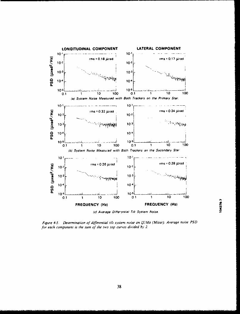
4-4 Samples of Tilt Power Spectral Densities Measured on 4UMa (Mizar) 36

4-5 Determination of Differential Tilt System Noise on 4UMa (Mizar) 38

4-6 Comparison of Differential Tilt Measurements Under Normaland Flipped Conditions 39

4-7 Turbulence Profiles Used for Numerical Calculations 40

4-8 Atmospheric Coherence Length ro Implied from aUMi (Polaris) TiltDuring Five Summer Nights 41

4-9 Isoplanatic Angle 0o at the Firepond Site During Five Summer Nights 43

4-10 Differential Tilt as a Function of Atmospheric Coherence Length 44

4-11 Tilt Anisoplanatism as a Function of Isoplanatic Angle 45

4-12 Tilt Anisoplanatism as a Function of Path Separation Comparedwith Calculations Based on Several Atmospheric Models 46

4-13 Tilt Anisoplanatism as a Function of Path Separation Normalizedto Atmospheric Coherence Length and Isoplanatic Angle 48

4-14 Ratio of Longitudinal and Lateral Components of Tilt Anisoplanatismfor Firepond Data 50

4-15 Location of Albany, Portland, and Chatham Weather Stations withRespect to Firepond 51

4-16 Wind Profiles at Albany, Portland, and Chatham During the Eveningof 10 June 1986 52

4-17 Power Spectral Density of Total Differential Tilt of 4UMa on theEvening of 10 June 1986 Compared with Theoretical Calculations 53

4-18 Typical Power Spectral Densities Taken During the Evening of10 June 1986 on the Double-Star ;UMa (Mizar) 55

4-19 Power Spectral Density tor Three Double-Star Separations forLongitudinal and Lateral Components During the Evening of10 June 1986 56

"Vill

LIST OF TABLES

TableNo. Page

3-1 Tracker Noise Characterization Using Test Source 19

4-1 Summary of Measurements of Double Stars 32

4-2 Atmospheric Parameters for Five Turbulence Models 40

ix

MEASUREMENTS OF TILT ANISOPLANATISMAT THE FIREPOND FACILITY

1. INTRODUCTION AND SUMMARY

The turbulence-induced wavefront aberrations seen by a telescope can differ significantly overtwo propagation paths with only slightly different propagation directions. *rhis is of particularconcern in adaptive optics systems where the beacon which is used to measure the atmosphere-induced aberrations is not viewed in exactly the same direction that compensation is to be per-formed. Friedl has shown that significant degradation in antenna gain is experienced in adaptiveoptics systems if the separation between the sensed path and the corrected path is large as com-pared with the isoplanatic angle, the angle over which the atmosphere irtroduces a constantphase change. The differences in atmospheric aberrations over these paths is known as the phe-nomenon of anisoplanatism.

In this report, we deal with the lowest order of anisoplanatism, that is, the differential tiltinduced by the atmospheric turbulence between two objects separated by a small angle. We callthis tilt anisoplanatism. The tilt anisoplanatism is a random phenomenon. For small path separa-tions its magnitude increases with path separation and it is independent of wavt,.ength. Whilelarger-aperture systems provide some aperture averaging for tilt anisopianatism, it is most bother-some in largc-aperturc short-wavelength systems whose diffraction-limited beam width is small.For instance, tilt anisoplanatism linii's the field-of-view of a high-resolution astronomical guidingsystem where a bright star is tracked to stabilize the telescope close to the dim star which isbeing observed. When working with satellites, laser radars and communications systems areaffected by tilt anisoplanatism because the transmitted beam has to be pointed ahead of thereceived tracker beam in order for the transmitted beam to intercept the satellite.

Lincoln Laboratory has investigated tilt anisoplanatism by observing binary stars (two starsseparated by a very small angle) with the 1.2-m-diam. Firepond telescope and measuring the dif-ferential tilt introduced by the atmosphere. Precision tracking equipment was construced to trackeach of the double stars of a pair. The differential tilt was obtained directly from the differenceof the tracked st.r positions. The results unfortunately show a factor-of-3 higher magnitude oftilt anisoplanatic error than previously believed.

1.1 HISTORICAL BACKGROUND

For over a half-century, astronomers have known of the harmful effects of what is nowcalled tilt anisoplanatism. This effect manifests itself when observing weaker star fields while thetelescope's line-of-sight is stabilized on a brighter guide star. As the radial distance from theguide star increases, there is a gradual decorrelation of the instantaneous position of the starimage. Serious limitations are thus imposed on the usefulness of a high-bandwidth guiding system

to steady all the stars within a wide field-of-view. On the other hand, improvement in the overallresolution of up to a factor-of-2 can result within a small field during planetary and double-starwork. Beyond this so-called isoplanatic patch size, the effectiveness of tilt removal falls away anddiscernible differential motion is present even at the edge of a planetary disk. This can be easilyseen by experienced planetary observers as rapid disk distortions and apparent displacement rip-ples of separate lunar crater images.

Dr. Frank Schlesinger, 2 an early in, estigator in seeing effects, noticed in 1927 that photo-graphic images of trailed stars showed almost parallel motions. This region of high positioncorrelation was referred to as a "parallax field." The small differential displacements observed inhis measurements were dismissed as measurement errors! In 1956, while developing a fast "seeir.gcompensator," J.H. DeWitt, R.H. Hardie, and C.K. Seyfe-t 3 proposed using their new device tomeasure the "coherence of seeing." They proposed to steady the image of Jupiter and observe theposition fluctuations of its satellites at various angular separations from the planet. Unfortu-nately. the results of this proposed measurement could not be found. In any event, the differen-tial motions thev were to measure are quite apparent when visually observing the planet Jupiterand its moons.

The nagnitude of differential tilt is closely related to the turbulence strength at high altitudeswhere the paths to the two stars do not overlap. In the early 1960s, A.H. Mikesell of the USNaval Observatory set out to measure high-altitude turbulence strength. Mikesell 4 used a portablehigh-bandwidth scintillometer which could be easily aimed at stars from an aircraft. His mea-surements demonstrated that, even at 37,000 ft, one-fourth of the twinkle amplitude remains. Thishas bccn confirmed by the fact that balloon flights instrumented for the purpose of high-resolution photography of the sun required altitudes of 80,000 ft and more to get above harmfulseeing disturbances.

Given these findings it was not surprising that, in our early experiments, we observed strongeffects of tilt anisoplanatism for binary stars of only 108-prad separation. While none of the earlyastronomical observations addressed quantitatively the magnitude of these effects, we attemptedto measure directly the magnitude of the differential tilt. These :'litial measurements at thle Fire-pond Facility in Westford, Massachusetts used two existing TV trackers and showed a sizable tiltanisoplanatism, which was much higher than would be predicted by commonly used atmosphericmodels. The accurac) of these measurements was poor and the measurement bandwidth waslimited by the TV frame rate to "-15 Hz, so we decided to buil!d suitable tracking equipment andto repeat the measurements with greater precision. This report describes this experimental systemand the results of the measurements.

1.2 EXPERIMENTAL EQUIPMENT

Two quad trackers were built for measuring tilt anisoplanatism. Each tracker used an opticalpyramid to divide the image into four quadrants, whose intensities were measured with photo-multipliers and combined to generate the beam-position error signals. The error signals were usedto drive a fast steering mirror in front of the optical pyramid to center the star image on the

2

detector system. The sum of the fast steering mirror position and the residual tracker erro,, .,!nalwas used as the estimate of the tilt seen by the tracker. Two similar trackers were constructed tolook through the same telescope, so that the pointing jitter of the telescope would cancel in thesubtraction process to obtain the differential tilt. The remainder of the optical system was con-structed to minimize uncommon jitter, for instance, by paying attention to thermal turbulencearound the optics and stability of the mounts.

The equipment was constructed, functionally checked out, and the first double-star differen-tial tilt measurements were made in the summer of 1985. While these data were of much higherquality than the initial TV measurements, the sensitivity of the system fell short of what wasexpected. Several improvements were made to the tracking system, including modifying the opti-cal setup and reducing the levels of various noise sources. In parallel with these modifications, ascintillometer was designed and constructed so that the isoplanatic angle could be measured dur-ing data taking. These improvements were incorporated into the experimental system in early1986. and the system was ready to collect tilt anisoplanatism data on double stars in the summerof 1986.

Measurement of tilt anisoplanatism requires the measurement of very small differential tiltfrom two stars, and consequently requires sophisticated tilt tracking equipment. Because of this,a considerable portion of this report describes the hardware that was designed and built for thispurpose. Sections 2 and 3 describe the design details and performance of the experimentalequipment. A reader not interested in the details of equipment can proceed directly to Section 4where the experimental results are presented. A brief review of the most-significant findings isgiven belowg.

1.3 SUMMARY OF RESULTS

Figure I-I shows -o-axis differential tilt measured on three binary pairs with separationsranging from 48 to 108 prad. The zenith normalized differential tilt is plotted against the normal-ized star separation. On the same figure are plotted values of tilt anisoplanatism, calculated bythe Optical Sciences Company, using various atmospheric models. We note that all the measureddata are higher than the SLC day model predictions but are bounded on the high side by theHV-5A model calculations, except for a few data points. (The SLC and HV models are described!atet in this ICport.) Note also that the tilt anisoplanatism magnitude is a large fraction of amicroradian for 50-prad star separation. which ii the maximum lead-ahead angle for low-altitudesatellites. This is much iarger than the usually quoted value of 0.3 jurad as calculated by use ofthe SLC models. Since the estimated measurement error is less than 0.2 prad. it cannot accountfor the large difference.

The two-axis differential tilt shown in Figure I-I is made up of unequal components alongand transverse to the star separation direction. Theory predicts that the longitudinal componentis the square root of 3 times greater than the lateral component for weak turbulence strength.Our measurements consistently showed a ratio of approximately 1.2, which would be the trendfor \ery strong turbulence levels.

S20

C) HUFNAGEL-VALLEY 54I°)" 15

A C)O~ C) CHUFNAGEL.VALLEY 27100

Zz SLC DAY

05A 1--- --

S00_ 0 50 _'o 150 200

DOUBLE STAR SEPARATION, Osec U/i (jlrad)

Figure 1-1. Differential tilt measured on double stars as a function of normalizedstar separation with calculations using sev'eral atmospheric models.

101

zw4.0-z:Z Lj

> ~HUF NAGEL VALLEY

I->

45S01

Z x

x= O0 S DAYU." 0 5 0 5 0

> HUFNAGEL-VALLEY(C 27

NORMALIZED PATH SEPARATION. 0 10/0o)/(D/ro) i

Figure 1-2. Tilt anisoplanatism as a function of path length nn rmalized to atmosphericcoherence length and isoplanatic angle.

4

__ _ _ _ _ _ _ __ _ __o_ _ __ _ _ _ _ _ _ _

During an experimental run, we also measured the isoplanatic angle and atmospheric coher-ence length on Polaris by observing its scintillation and angle-of-arrival jitter. Figure 1-2 showsthe tilt anisoplanatism normalized by the tilt variance to a single star of the pair plotted as afunction of star separation normalized by the isoplanatic angle 00, the atmospheric coherencelength ro, and the telescope aperture diameter D. Note that when the theoretical predictions areplotted in this normalized fashion, the curves for all models fall roughly on top of each other.Here, the measured data correlate much better with the predictions based on the various modelsWhile the tilt anisoplanatism values were much higher than predicted, the measured 00 and rocorresponded to a stronger turbulence than modeled. Thus, we must conclude that the turbulencestrength in the vicinity of the Firepond site is much stronger than predicted by the SLC model.

The power spectral density of tilt anisoplanatism is dependent on the high-altitude windvelocity. Our measurements showed that the shape of the power spectral density could changefrom minute to minute. However, the measurements also show that most of the tilt anisoplana-tism energy occurs at frequencies less than 30 Hz and the energy above 100 Hz is almostnegligible.

5

2. EQUIPMENT DESCRIPTION

The overall block diagram of the tracking system is shown in Figure 2-1. The system consistsof the Fircpond mount for following the double-star motion, two trackers (each having a quaddetector and a fast steering mirror), and recording and associated data-gathering equipment.While the Firepond telescope is pointed in the general direction of the double star, each of thetrackers is locked-on to a separate star. The optical bias blocks (prisms) are in the system to shiftthe line-of-sight of each tracker to either of the stars. Since the quadrant detectors have atransfer characteristic which is dependent on the image size (which, in turn, depends on theatmospheric seeing that changes from minute to minute), the system has a fast steering mirror infront of each tracker which was used in a closed loop to track the angle-of-arrival to minimizethe quad detector output. By adding the smafl residual crror indicated by the quad detector out-put to the fast steering mirror position, the quad detector calibration uncertainty due to spot sizeis minimiied. The output of the quad trackers and the fast steering mirror positions are recordedon the computer tape at a 4-kHz rate and processed for ýarIous statistics post-mission.

DOUBLE.........

3": ..... - • "PYRAMID

"BEAM -,PMfS

/i

/ " TV QUAD •

SII ISERVO!

Sb

- FM -IlFSM [SERVO.

S, II I LOOFIREPOND 48 INCH L O "

TELESCOPE BIAS BLOCKS_____

S....COMPUTER/ MAG AND MOUNT -, ..

S( APE DRIVE MIRROR POSITION, QUAD DETECTORSIGNALS, SIGNAL AMPLITUDE

'iRure' 2-1. Jilt arlu.)plafl% ..•u f•l ew'.;r•fl•t f uqn• mot' .I/ /I.S - /'cUtit sp)!I1I'r. F..f /a.i .leering

mflirror, F'M z fold nhurror, PAM -- ;p itoniultiptr /I!'c)

7

2.1 FIREPOND 1.2-m TELESCOPE SYSTEM

The Firepond telescope, shown in Figure 2-2, has a 120-cm aperture and a 13.8-cm secon-dary mirror. The secondary mirror can be tilted in two axes for faster angle tracking to com-pensate for mount dynamic lag and for jitter. The secondary mirror can also be adjusted with aservo to focus at different ranges. The mount angular velocity and acceleration capabilities aregreater than 101:s and 100-s2, which is adequate for tracking low earth-orbit satellites. The Fire-pond telescope is described in Reference 5.

One of the main attributes of the mount is its extremely smooth control system. Both azi-muth and elevation axes are supported by ball bearings and are driven by direct gearless dctorque motors. The mount position, reported by 24-bit optical angle encoders, is subtracted fromthe mount commands in the control computer and the difference, after compensation, is used todrive the mount. The amplification of drive signals is accomplished by controlling the field cur-rent of dc generators driven with a 60-Hz motor. While there are several servo modes, normallythe system is used in Type 11 software compensation mode. In this mode, the closed-loop servobandwidth is -2 Hz in azimuth and '- I Hz in elevation. The secondary mirror tip, tilt servos,whose clcsed-loop bandwidth is '-25 Hz, can be used to widen the pointing bandwidth in severalcascade pointing modes. The secondary mirror is supported by a flexure pivot and tipped andtilted with dc motor-driven lead screws. Secondary position is reported by LVDTs (Linear Vari-able Differential Transformers) with a resolution of ±0.375 jirad.

100

Filzure 2.-2. E-rcpond I -ni-aperiure tele¶iiope A ith the 60--ni-aperture finder tele.icope.

• I I II I I

The telescope is controiied by two Gould SEI, 32 27 computers. Various modes of pointingare available under software control. During the tilt anisoplanatisn, measurements, a FK-4 starcatalogue containing '-1600 stars was used to point the telescope toward a desired double star,and small-angle biases were added through handwheels to position the star in the field-of-view atthe desired spot.

A 60-cm Newtonian finder telescope is mounted on top of the Firepond 120-cm telescope.An I 1-cm-diam. patch of this telescope aperture was used for the scintillometer (described later)which we used to measure the isoplanatic angle during the double-star tracking experiments.

The telescope is housed in a dome which is slaved to the telescope azimuth. The dome pro-vides good protection against disturbances and biases caused by wind and sun loading on thetelescope.

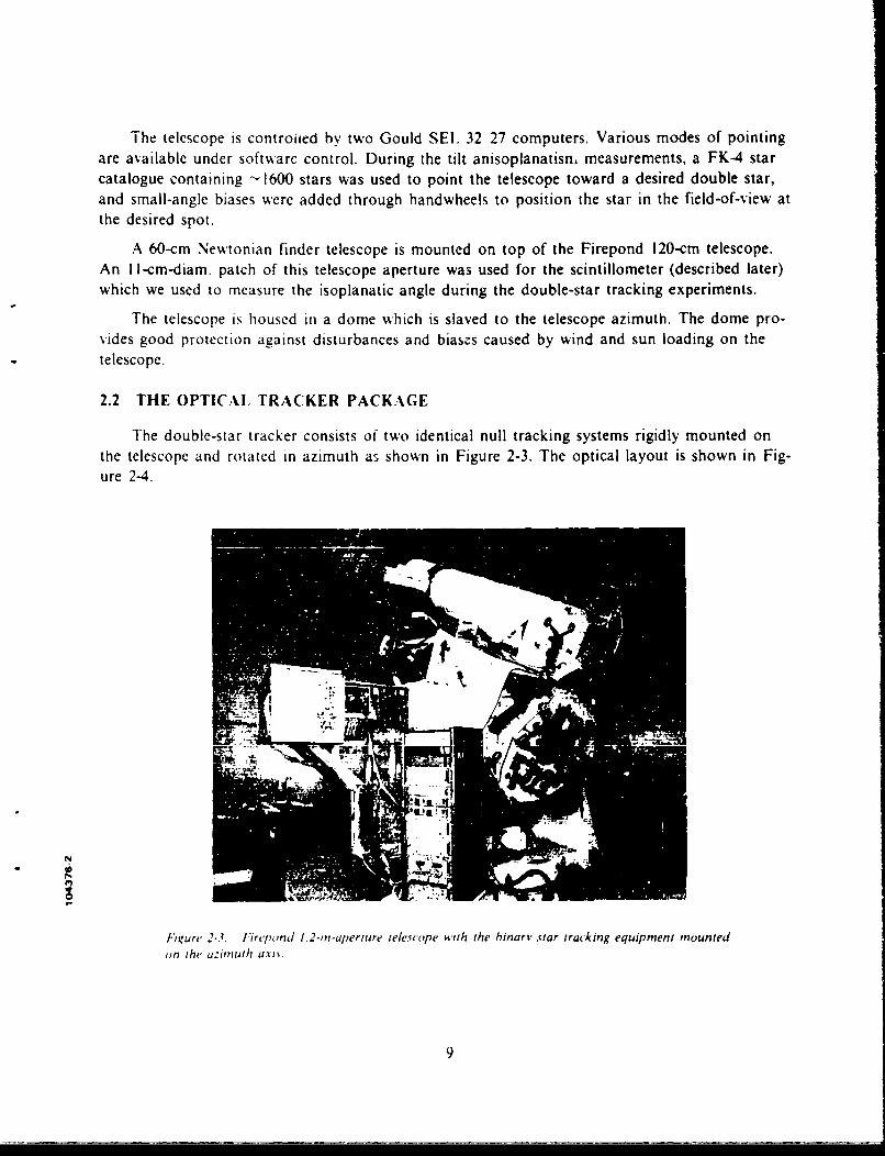
2.2 THE OPTICAl, TRACKER PACKAGE

The double-star tracker consists of two identical null tracking systems rigidly mounted onthe telescope and rotated in azimuth as shown in Figure 2-3. The optical layout is shown in Fig-ure 2-4.

Ni

Ftiure 2-.. Iirepond 12-m-aperture telescope with the binary star tracking equipment mountedon Mhe auonmuth a.xt•.

9

CORRECTORPLATE/

ENTRANCE TV1.2 m TELESCOPE WINDOW

S~~~TRANSFER LENS CLIAO

COLLIMATORMIRROR

45/55 FSM No. 1DIELECTRIC BS FELSTP

FIELD STOPS

F/63 BEAM TRK No. 1

M NPYRAMIDBIAS BLOCKS

F/63 BEAM TRK No. 2

PYRAMID

Figure 2-4. Optical schemnatic of hinarY star tracker.

For this experiment, the Firepond telescope was configured as an f, 32 Cassegrain, which is a

departure from the normally used f. 200 Cassegrainian configuration, with a consequent increase

in spherical aberration introduced by the system. This aberration was corrected with a small

fused silica corrector plate located 47 in before the focus. The corrector was null figured in situ

using Polaris as the test source. The corrector also served as the input window to the thermally

insulated optics package.

The first component in the optical package is a thin-film beam splitter (a pellicle) that

reflects 2.5 percent of the light through a transfer lens into a sensitive intensified silicon intensi-

fier target (ISIT) camera which is used to guide the star image into the field-of-view of the

trackers. This TV also provides the position angle of the binary pair in the tracker coordinates,

so we may identify the longitudinal and lateral measurement axis for data-reduction purposes.

The transmitted divergent beam is collimated by a spherical mirror that also re-images the 1.2-m

entrance pupil into the exit pupil plane well beyond the next element. The astigmatism intro-

duced by the spherical mirror is corrected with a special mounting cell for the spherical mirror

which introduces astigmatism of the opposite sign with sufficient piecision that diffraction-limited

performance was easily achieved.

10

The next element is the 45/'55 beam splitter. From this point in the path, the collimatedbeams proceed to each tracker. Great effort was expended to ensure that the trackers were op-tically identical and to ensure that each would have identical image and magnificationcharacteristics.

The next element in each path is the spherical fast steering mirror with a focal length of92 in. This focal length was chosen to provide a blur circle large compared with the pyramid tipblunting errors, as well as having sufficient depth of focus at the field stop which must be posi-tioned slightly ahead of the prism tip. The convergent beam next passes through the bias blockswhich provide a means of fine steering or offsetting the final lateral position of the focal spot.This is necessary for selecting either the primary or companion of the binary star. The biasblocks are mounted in a roll (position angle) and tilt (separation) servo-driven cage controlled bythe console operator. Typically, both bias blocks were tilted to share the displacement valuemaintaining the best focus. Tilting the blocks introduces only trivial aberrations, 100 timessmaller than the typical seeing disk.

The quad error sensors are shown in Figure 2-i. A highly reflective pyramid, shown in Fig-ure 2-6, divides the focal spot into four beam segments which are directed to four EMI Model9826 photomultipliers. The photomultiplier tubes have a bialkali photocathode which has its peakquantum efficiency at "-0.35-Azm wavelength. The faces of the photomultiplier tubes are tilted atslight angles to prevent reflections into opposite tubes. A circular stop is mounted in front of thepyramid to admit only one star intc each quad sensor. This aperture is drilled to subtend 37 /rad,which is small enough to separate star pairs but large enough to admit the full seeing blur.

.j .. .......... ...

Figure 2-5. Quad detector with four photonultiplier tubes.

II

Vp ..

Figure 2.6. Quad detector pyramid and circular stop.

2.3 THE FAST STEERING MIRROR

The fast steering element is a 5-cm-diam. mirror, mounted on a ring which is supported by

three flexures and driven by three piezoelectric actuators. Four linear variable differential trans-

former (LVDT) sensors are spaced at 900 intervals along the ring to provide elevation and azi-

muth readings of the mirror position. We chose the lead-zirconium titanate (PZT) actuator-driven

fast steering mirror for keeping the target image on boresight, as it most clearly guaranteed a

performance level margin for the experimental program. PZT actuators are capable of high-

frequency response; our mirror and driver can typically achieve a frequency response of 500 Hz

in closed-loop mode.

Construction details of the mirror are shown in Figure 2-7. The mirror is driven by three

PZT units spaced 1200 apart. This arrangement prevents mechanical overconstraint. The 3-axis

motion is resolved into two mutually perpendicular axes electronically.

Four LVDT core pieces, one for each transformer, are bolted to four symmetrically dis-

placed extension tabs on the mirror edge. These tabs are in the plane of the mirror surface. The

coil portion of the LVDTs is mounted to the fixed-mirror support stand and is adjustable along

the measuring axis, thus providing a means of nulling the output voltage at the zero tilt position.

The 5-cm-diam. mirror is machined from a solid aluminum billet, stress relieved, and nickel

plated before optical surfacing and high-reflectivity coating. Since final focusing is accomplished

with these mirrors, they are finished with a shallow concave spherical surface of 184-in radius.

12

PZT ALIGNER/TRANSLATOR

LVDTT

STATOR R

NULL SCREW CORELVDT ••

MIRROR

S( • I•----MIRROR

BURt_FIGH •

ASSY

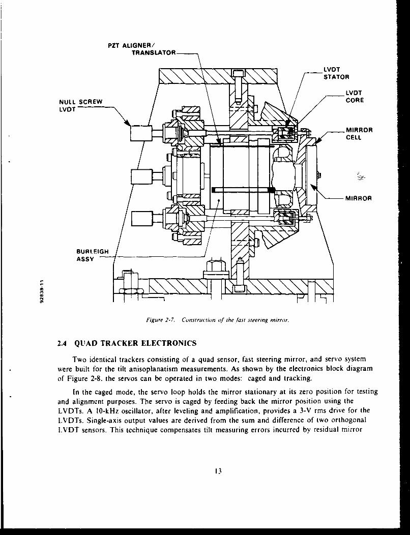
Figure 2-7. Construction of the fast steering mirror.

2.4 QUAD TRACKER ELECTRONICS

Two identical trackers consisting of a quad sensor, fast steering mirror, and servo systemwere built for the tilt anisoplanatism measurements. As shown by the electronics block diagramof Figure 2-8. the servos can be operated in two modes: caged and tracking.

In the caged mode, the servo loop holds the mirror stationary at its zero position for testingand alignment purposes. The servo is caged by feeding back the mirror position using theLVDTs. A 10-kHz oscillator, after leveling and amplification, provides a 3-V rms drive for theLVDTs. Single-axis output values are derived from the sum and difference of two orthogonalLVDT sensors. This technique compensates tilt measuring errors incurred by residual mirror

13

TRANSIMPEDANCEAMPLIFIERS

PIVIT A

1ATPMT 6

PMT C

IF

OSCILLATOR 4 PMT D

P A IMPEDANCE

LEVELER SFIECTOR

SHIF YER

3 V SINE WAVE

LV., A.ýLIFIERS DIFFERENCEAMPLIFIERSDIFF1 RE NVC1 S.'(;YERA.PL AS

PLI11E

CAGE TRACKF1 -tLPF

LPFLVDT

No 3 EAIIUR

A, A, TOOAS

ERRORTO

LVOT OAS -40-41

Lý OFF CONTROL

SYNLHRONOUSDETECTOR

MODE BAN D WIDTHS ELECTOR SELEC70R

INTEGRATORS

PMIF A PMT 6In LVOT No I HIGH VOLTAGE

2TO AXIS AMPLIFIERS'YV RTFR HVA

STK RATE SIK

LvDT No 2 LIMITER EDN-, .4 LVUI No 2 NVA STK

RATE

SIK No I SYK No J LIMITER No 2

7,'ýVA SIK 44

LVOT No 3 RA

MT 0 PMT C 97

I TERMý No ISUALE-GH

DRIVERS C4

Figure 2-8. Quad tracker electronics. (DA S Data-A cquisition S -v-stem, LPF = low-pass filter,L VD T = linear variable differential transformer, PAI T = photomultiplier tube).

14

translation. Synchronous detection of the LVDT outputs allows the magnitude and the direction

of the mirror position to be determined. After filtering and amplification, the detector outputsprovide a voltage proportional to mirror motion with 16.5-mV, prad angular responsivity. These

position signals are fed into the servo system compensation circuits to keep the mirror position atthe nominal zero position. Since the LVDTs produce an azimuth and elevation mirror positionsignal, but the mirror drive is accomplished by three PZT stacks, a 2- to 3-axis converter circuitis used before the rate limiters and high-voltage stack drivers.

In the tracking mode of operation, the error signals are obtained from the quad sensors. Thephotomultiplier tube output currents are converted to voitages by transimpedance amplifiers.Three values of load resistance can be selected to compensate for the variation in stellar bright-ness. Azimuth and elevation position error signals are obtained by combining sum and differencesignals as shown in Figure 2-8. By normalizing the differences with respect to the sum, positionerrors independent of the stellar brightness are obtained.

In either the caged or the tracking mode, the servo tries to null the error. Varying the gainof the amplifiers preceding the integrators in the Type I loop adjusts the bandwidth of the servo

response. The linear control of the servo can provide a maximum safe voltage of 1000 V to theactuators. which corresponds to ±1 18 prad from the mirror center position or ±10 prad in thesky coordinates.

2.5 TRACK-DATA-ACQUISITION SYSTEM

The Firepond control computer collects system status data and records them on magnetictape for post-mission data analysis. Numerous data items are sampled at various data rates andorganized into tenth-second-interval data blocks for recording. The double-star experiment uti-lizes this feature for data collection. Since the normal Firepond real-time sampling rates are not

high enough, a new data-acquisition system was built to collect the tracking data at a 4-kHzsampling rate. This systera samples the mirror positions, quad detector outputs, and star signalamplitude for both trackers.

Figure 2-9 shows the block diagram of the new Data-Acquisition System. The ten channelsof data inputs are smoothed with 5-pole Butterworth low-pass filters with a -3-dB cutoff atI kHz to suppress aliasing. Then, all ten channels are sampled and held simultaneously at a4-kHI rate. Between samplings, an analog multiplexer delivers the data to the 12-bit analog-to-digital converter which feeds its outputs into a FIFO (first-in first-out) memory. The contents ofthe FIFO memory are transmitted to the computer in a direct-memory-access mode via a multi-purpose interface card capable of a throughput of I Mbytejs. The 4000-S,!s per channel samplingrate is well within this capacity. These data are buffered into tenth-second data blocks and re-corded on magnetic tape along with other Firepond system parameters. The start and end of thedigitization and data recording are controlled by the operator.

Various data processing and analysis programs are available for analyzing the Firepondrecorded dmta. These programs were utilized in the double-star data analysis as well. Several new

15

CHIAN. 1 &

DATA /

IPTMPU(R CONV. FIFO DATAI (= OUT

CHAN. 10J

LINE t tt CN.DRIVERRCVR ~ ADDRESS COMML

1 -7,RCVR1 MHz - - -Uj

CLOCK ADDRTESS

MODULO NTOFROM RTP

0 L F0

ONgu E RESE AaaA=Bsln Ssm LF Iwpa~ itr & sml odSHO- T fiOUt-iR firMtoutAeTOR

16S

processing programs wert. required for the processing and analysis of the differential tilt data.The experiment-related software operated in two phases: In the first phase, various statistics andparameters were computed for individual data-collection runs. The second phase entered thesedata into a double-star data base where additional conversions took place in order to present thedata and statistics in a convenient form. The results section gives a reasonable sample of theresults which were obtained by the use of these software.

2.6 STELLAR SCINTILLOMETER

During checkout runs, we observed that on nights when star twinkle was strong, the differ-ential tilt was also large. These observations quickly led to the design and construction of whatwe affectionately call the "twinkle meter." The twinkle meter simply measures the star light scin-tillation with an I l-cm-diam. aperture. Loos and Hogge, 6 have shown that an I l-cm-aperturescintillometer weights the atmospheric structure function (C2) with altitude in approximately thesame manner as the isoplanatic angle. Thus, the scintillation amplitude can be measured andconverted directly to isoplanatic angle, as described in Section 4.5. The twinkle meter shared aportion of the 60-cm Newtonian Finder, which rides atop the main telescope. The field-of-viewof the scintillometer was limited to 100 prad to view only one star.

The block diagram of Figure 2-10 shows how the instrument works. Light falling on thephotomultiplier is converted to an electrical signal which is amplified and separated into its dcand ac components. The true rms-to-dc converter provides a voltage proportional to the ac fluc-tuations of the stellar brightness. The dc component is proportional to the brightness. The ratioof the two components is scaled so that 10 V corresponds to 100-percent modulation.

17

HI rs TOFLUCTUATION

PHOTOMULTIPLIER LN

r_1BRIGHTNESS

APERTURE AMPLIFIER AND

(% Modulation)

> RAW SIGNAL

LINE DRIVERS 'TO RECORDERS

Figure 2-10. Twinkle meter schematic.

18

3. SYSTEM PERFORMANCE

Because the expected values of tilt anisoplanatism are small, its measurement requires a pre-cise and well characterized instrument. The important characteristics which determine the accu-iacy of the measurements are system sensitivity, bandwidth, and angle calibration. This sectionsummarizes the test results of a few of the many tests that were performed. The techniques ofsystem calibration before data-taking sessions are also described.

3.1 TRACKER NOISE SOURCES

A total system noise of 130 nrad (referenced to the sky space) was directly measured for a4th-stellar-magnitide equivalent light source. Table 3-1 shows the measured or estimated magni-tude of tle various sources of noise.

TABLE 3-1

Tracker Noise Characterization Using Test Source(0.5- to 100-Hz Bandwidth)

NoiseError Contributor Method (nrad rms)

Unshared Path Turbulence Measured 24

Total System Electronics Measurec, 9

Pyramid Blunting Computed 20

Focus Error Computed 10

RSS 34

Using a bright point source (about 0th-magnitude equivalent) located at the Cassegrainiantocus with the telescope pointed out in an operational condition, we found that unshared pathdisturbances originating within the optical train contributed 24 nrad. The extra bright sourcereduced other noise sources, such as photomultiplier tube noise, to a negligible value. A veryshort and harmless unshared path region could not be measured. This region is just a few cen-timeters of path before and after focus, where the separate cones of light emerge as separatebeams and form the closely spaced images of the double star and then recombine. Because thispath is sealed with the corrector plate and insulated with the same care as the entire package, wefelt that this region contributed a negligible error.

19

The electronic noise was measured to be 9 nrad by shorting the input to the transimpedanceamplifiers and processing the output noise. The centroid determination errors due to pyramidblunting and defocusing were estimated at 20 nrad.

These measured and estimated noise components are small when compared with total mea-sured system noise of 130 nrad, which implies that the main contributor is the photomultipliernoise. The photomultiplier noise was estimated to be 124 nrad by subtracting the other noisesources from the total measured system noise. We were unable to confirm by calculations thatthese implied noise levels should be expected, because we did not have the exact gain characteris-tics of the photomultiplier tubes and precise knowledge of the optical transmission.

These low noise values were never observed while tracking 4th-magnitude stars because starimages are typically 10- to 15-Mrad diameter and beset with scintillation and high-frequency shapedisturbances. However, the actual noise level under average seeing conditions is low comparedwith the typically measured differential tilt. During the experiment, the noise was estimated fromcontrol measurements (when both trackers tracked the same star) and was subtracted from thedata, as explained later.

3.2 ULTIMATE BANDWIDTH AND NOISE-FLOOR TESTS

Both closed- and open-loop performance testing of the tracker and fast steering mirror sys-tem was performed at our optics test facility where we set up and tested the fast steering mirrorsand electronics as they would be used in the final optics package. Each mirror was, in turn, pro-vided with a collimated input beam and the reflected convergent beam was focused on the quadphotomultiplier error sensor as shown in Figure 3-1.

PYRAMID PRISMFIELD STOP

PLYWOOD BOX

' PMT2 (4) 12" COLLIMATOR

FSM

APE RTU E .f•= u

SELECTABLEAPERTURES (Pinholes) FOCUSING LENS

I/INCANDESCENTS RSOURCE

Figure 3-1. Test setup for quad trackers.

20

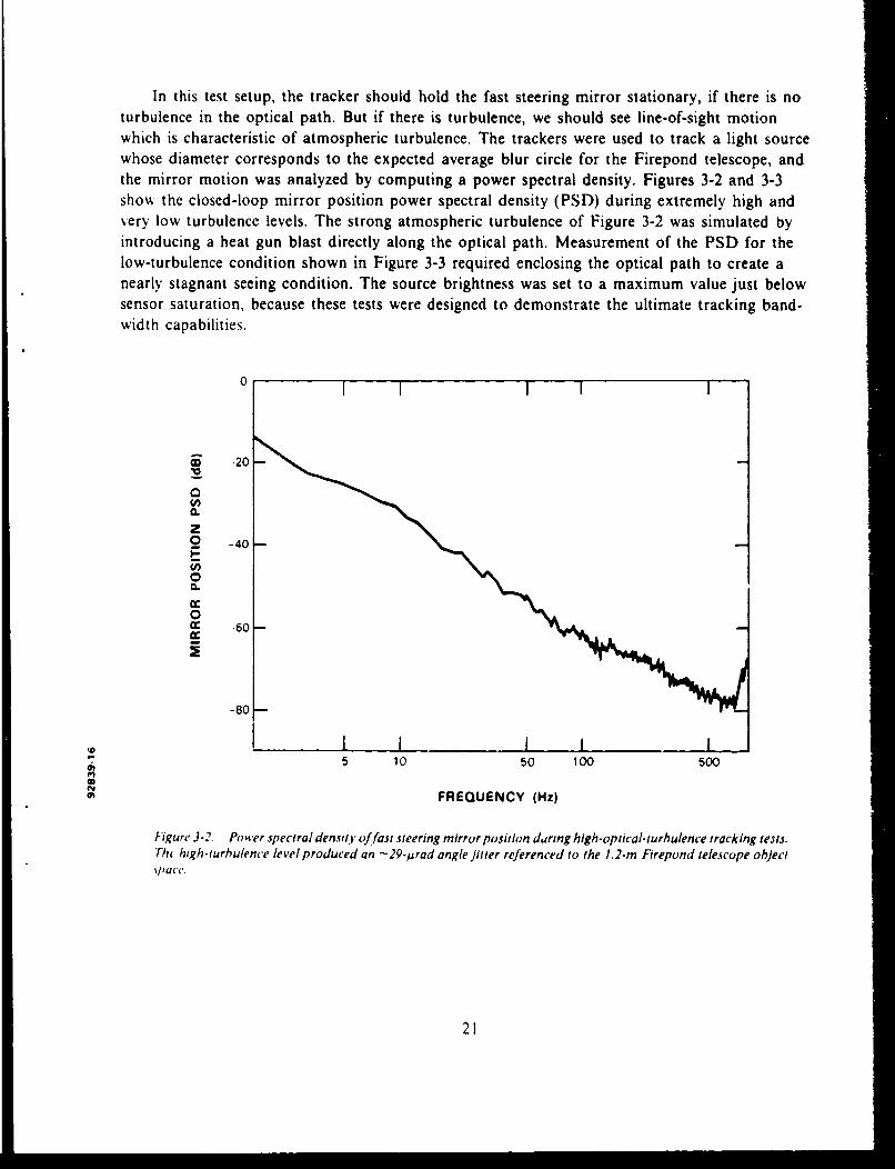
In this test setup, the tracker should hold the fast steering mirror stationary, if there is noturbulence in the optical path. But if there is turbulence, we should see line-of-sight motionwhich is characteristic of atmospheric turbulence. The trackers were used to track a light sourcewhose diameter corresponds to the expected average blur circle for the Firepond telescope, andthe mirror motion was analyzed by computing a power spectral density. Figures 3-2 and 3-3shov, the closed-loop mirror position power spectral density (PSD) during extremely high andvery low turbulence levels. The strong atmospheric turbulence of Figure 3-2 was simulated byintroducing a heat gun blast directly along the optical path. Measurement of the PSD for thelow-turbulence condition shown in Figure 3-3 required enclosing the optical path to create anearly stagnant seeing condition. The source brightness was set to a maximum value just belowsensor saturation, because these tests were designed to demonstrate the ultimate tracking band-width capabilities.

S.20

0

0.

o -40 -

cc

0

cc -60-

-80

.oII I I I

-5 10 50 100 500

FREQUENCY (Hz)

figur' 3-2. Power spectral density offast steering mirror position daring high-optical.turbulence tracking te3ts.Thc high-turbuience level produced an -29-prad angle jitter referenced to the 1.2-m Firepond telescope objectwatc.

21

-40

S-50

0

0

0

07

-80,

1 5 10 50 100

FREQUENCY (Hz)

figure 3-3~ Po wer s~pectral de'nsity of fast steering mirror position during optical tests with extremel "v losv-turhulent v level. This lo v- turhulences .irulat ton produced only -20 nradl of total angle jitter referenced to the1.2-rn Firepond telescope oblect space.

During these tests, the loop gain of the Type I servo was set as high as possible. We wereable to get loop bandwidths as high as 1000 Hz during these high-signal-level conditions. Notefrom Figure 3-2 that the first serious resonance is just beyond 800 Hz which is typical for eachaxis on both trackers. The low-turbulence measurement was performed to demonstrate the ulti-mate closed-loop noise-floor level on a nearly ideal stationary source. Note that the 60-Hz powerline interference which is evident at these low values of mirror motion in Figure 3-3 are hiddenin the high-turbulcnce measurement of Figure 3-2.

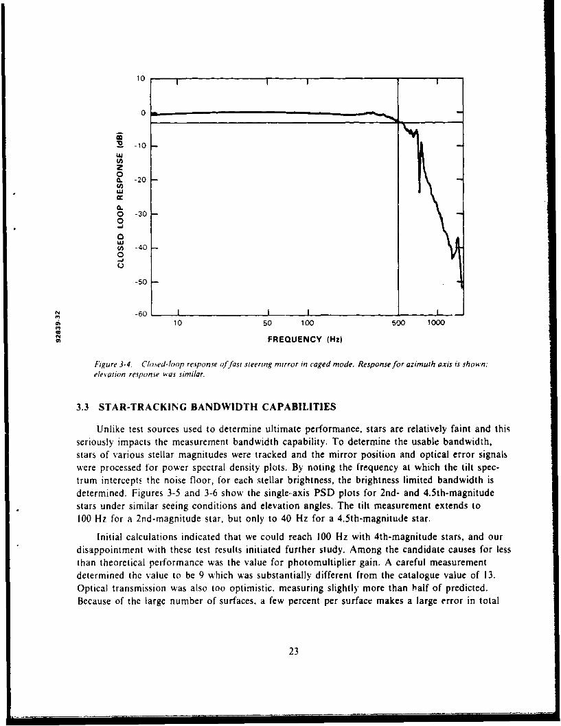
Caged mode tests were performed to meastire the phase shift inherent to this particulartracker. This mcasurcmcnt is important only if the mirrors were to be used in open-loop beam-pointing applications. Since the binary star experiment depends on subtracting one tracker posi-tion from the second tracker, phase errors are unimportant so long as they are closely matchedfor each tracker. It is of some interest that the 450 phase point under open-loop condition occursat 160 Hz. The measured caged mode mirror response curve is shown in Figure 3-4. A HP-3562analyzer was used to compute the transfer function between the fast steering mirror position andthe servo error signal while a random excitation was added to the servo error signal. Note thenear flat spectrum out to 500 HL and again thc resonance at 800 Hz showing, in this case, as adip (it can be either a small dip or peak depending on the exact servo filter characteristic).

22

10

0

S-10'U

0(. -20UC

a-o -300

(A -40 -0

-50 -

N -6I I

h 10 50 100 500 1000

0m FREQUENCY (Hz)

Figure 3-4. ChO.wed-loop response of fast steering mirror in caged mode. Responsefor azimuth axis is shown;elevation response was similar.

3.3 STAR-TRACKING BANDWIDTH CAPABILITIES

Unlike test sources used to determine ultimate performance, stars are relatively faint and thisseriously impacts the measurement bandwidth capability. To determine the usable bandwidth,stars of various stellar magnitudes were tracked and the mirror position and optical error signalswere processed for power spectral density plots. By noting the frequency at which the tilt spec-trum intercept, the noise floor, for each stellar brightness, the brightness limited bandwidth isdetermined. Figures 3-5 and 3-6 show the single-axis PSD plots for 2nd- and 4.5th-magnitudestars under similar seeing conditions and elevation angles. The tilt measurement extends to100 Hz for a 2nd-magnitude star, but only to 40 Hz for a 4.5th-magnitude star.

Initial calculations indicated that we could reach 100 Hz with 4th-magnitude stars, and ourdisappointment with these test results initiated further study. Among the candidate causes for lessthan theoretical performance was the value for photomultiplier gain. A careful measurementdetermined the value to be 9 which was substantially different from the catalogue value of 13.Optical transmission was also too optimistic. measuring slightly more than half of predicted.Because of the large number of surfaces. a few percent per surface makes a large error in total

23

11II

100 ATMOSPHERIC TILT JITTER

ALIASINGS102 FILTER -

".,. RESPONSEV

6 ILI

- 10_4 IflSYSTEM NOISECL -FLOOR

0-6S10-8

0.1 1 10 100 1000 10,000 CD

FREQUENCY (Hz)0.1J

Figure 3-5. Tilt power spectral density on a 2nd-stellar-magnitude star (mirror azimuth position plus residualquad detector error).

100 ATMOSPHERIC TILT JITTER

FILTER RESPONSE

12* -EM NOISE FLOORo 10-4

I-- 0.

10-8

0.1 1 10 100 1000 10,000

FREQUENCY (Hz)

Figure 3.6. Tilt power spectral density on a 4.Sth-stellar.magnitude star (mirror azimuth position plus residualqjiad detector error).

24

throughput estimate. In addition, all the reflectance measurements were made with a HeNe laserat 0.6 3 -Am wavelength, but our photomultiplier system has peak response around 0.35 Am. De-spite these shortcomings, good measurement capabilities eyisted and we proceeded with the data-collection task.

3.4 CALIBRATION OF THE OPTICAL ERROR SIGNALS

The angle-of-arrival to each of the binary stars was obtained during the double-star mea-surements by adding the fast steering mirror position and the residual quad detector sensor out-put. Calibration of both the steering mirror position sensors and the quad detector output signalsis important if precise measurements are to be obtained. Although inclusion of the residual errorsis unimportant at low frequencies, up to about 20 Hz for a 4th-magnitude star, its importanceincreases with wide-bandwidth measurements and is essential for data collection beyond 50 Hz.

Since the slope of the quad detector output voltage vs angle error depends on the size of theimage on the tip of the pyramid, this transfer curve is dependent on the atmospheric seeing con-ditions and must be calibrated for the particular seeing conditions during data-taking. This makesit very difficult to accurately determine the angle-of-arrival error implied by the quad detectoroutput and is the main reason why we used a fast steering mirror in front of the detector, so thatthe bulk of the angle-of-arrival measurement could be obtained from the fast steering mirrorposition and only a very small portion would come from the quad detector output voltages. Ifthe quad detector error signal is poorly calibrated (because the seeing conditions have changed),it will contribute only a small error to the total measured angle.

-1 he optical error voltage was calibrated with the optical tracker in the caged mode. In thismode, the fast steering mirror was electrically positioned stationary and aligned to the opticalaxis. Next, a star image was sinusoidally scanned in x and y across the pyramid tip by scanningthe Firepond telescope secondary mirror, and the error voltages were recorded. These scan testsemployed angle displacements of only a few microradians, since larger scan angles result in aSlightly nonlinear output vs angle. A 2nd-magnitude star (Polaris) was the test source for thesemeasurements. The measuremen, was performed only after the servo gain was adjusted for theparticular seeing condition of the test. This ensured a reliable value for the optical error voltagecalibration as this parameter is normalized (gain adjusted) before each binary star experiment totake into account night-to-night seeing variations. Often the gain had to be reset in a singlenight's run, since the seeing often stepped to a new strength level partway through the night.

3.5 ANGLE-OF-ARRIVAL CALIBRATION

Precise measurement of the differential tilt magnitude requires an exact calibration of thefast steering mirror LVDT voltage as a function of position. rhe angle-of-arrival tilt ctlibrationof the fast steering mirror consisted of five separate techniques, each of which was us( J forangle-of-arrival calibration in various phases of the experimental program. Three of thesemethods involved active optical tracking, and the remaining tests were of a rather indirect nature.

25

Rotating Light Source:- This test consisted of tracking a rotating light source, a small-filament 6-V clear bulb and attached lantern battery. The assembly was rotated at 7 rps using asmall dc motor. The bulb filament center was offset 2.25 cm from the rotation axis, thus produc-ing a circle of - 10-/Arad angular diameter as viewed by the telescope at a distance of 5.4 km. Theaxis of rotation was accurately aligned with the telescope line-of-sight, producing a true circle ofrotation in the telescope field-of-view. Recording and digitizing the peak voltage in each axis(x and y) provided a scale in terms of counts (volts) per microradian in the sky.

Secondary-Mirror Scans on a Star:- This method was an active star tracking test with tiltsintroduced with the calibrated Firepond telescope secondary mirror. Here, the secondary mirroris computer controlled with various optional scan functions such as a circle, raster, or simple xor y motion. These scan motions can be commanded over a wide range of excursions and rates.We operated mostly with a circle to match thM rotating light tests.

Input Focal-Plane Light Source:- In this test a point source, mounted on a precise x,y,ztranslation stage, was located at the input focal plane of the tracker package. The plate scale iscalculated for this point of the optical system providing a value in terms of Aradi'mm. Whileactively tracking the point source, the stage was translated, alternately, in x and in y by 10-pradsteps and the position voltage was recorded as in the previous tests.

Optical Magnification:- The optical magnification method infers the calibration value fromthe optical magnification and the fast steering mirror calibration. The test involved a photo-graphic measurement of the exit pupil diameter (see optical system description) to obtain theoptical magnification. This, when combined with the bench check values of the fast steering mir-ror (volts per microradian in fast steering mirror space) provides the calibration scale in objectspace.

Ray Trace:- A ray trace of the entire system was made to determine the system magnifica-tion which was applied to the bench test scale factors of the fast steering mirror as an additionalcalibration.

All five techniques agreed well, with a peak error of only 10 percent, and provided a nomi-nal calibration constant of 238 mV prad in azimuth and 247 mV prad in elevation at the analog-to-digital converter interface. We depended on the rotating light as our fundamental standard ofcalibration, and adjusted the secondary-mirror scanner values to agree. Routine checks during theexperimental program were performed with the calibrated secondary mirror.

3.6 TRACKER SCALE-FACTOR BALANCE

The two-axis closed-loop tracking method for the differential tilt measurement required thatthe two trackers respond identically to identical input wavefront slope variations. To balance thetracker position outputs, the analog gain was adjusted to equalize the outputs during a single-startracking test in which the secondary mirror was scanned in x and in y at 7 Hz with a peak-to-peak angle of 20 prad. A power spectral density of the mirror position was recorded for eachtracker axis, and the analog gains were adjusted to produce equal output voltages at the 7-Hzfrequency. This method, although providing excellent accuracy for ordinary use (-5 percent), leftresiduals larger than the I-percent design goal.

26

To further refine the tracker balance, the following technique was used. A point source lightpositioned at the input focus and mounted on an x and y translation stage was adjusted, in turn,to the field extremes with the tracker in closed-loop mode. The digitized values (counts) of thefast steering mirror position for each field position were recorded. Software scaling values werethen adjusted and applied to these data to bring both axes to equal counts. The resulting scalefactor was used in the data processing.

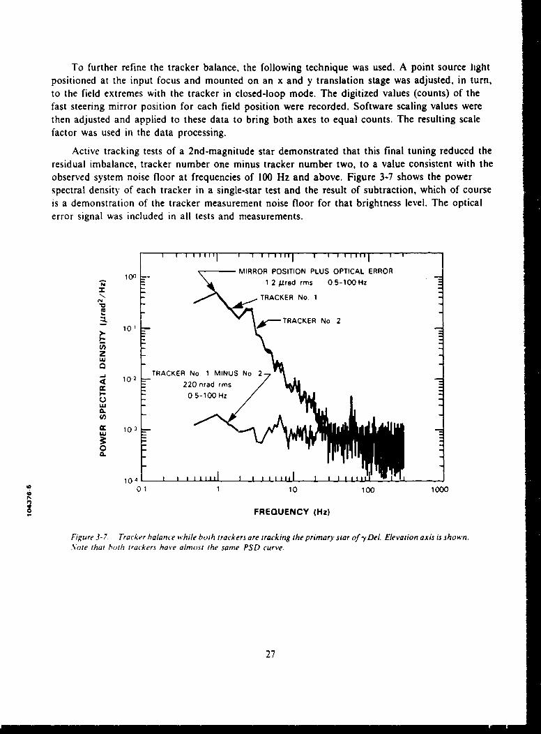
Active tracking tests of a 2nd-magnitude star demonstrated that this final tuning reduced theresidual imbalance, tracker number one minus tracker number two, to a value consistent with theobserved system noise floor at frequencies of 100 Hz and above. Figure 3-7 shows the powerspectral density of each tracker in a single-star test and the result of subtraction, which of courseis a demonstration of the tracker measurement noise floor for that brightness level. The opticalerror signal was included in all tests and measurements.

100- MIRROR POSITION PLUS OPTICAL ERROR

1 2 /p.rad rms 0.5-100 Hz

"N TRACKER No.1

S101 - TRACKER No. 2

Z

102 TRACKER No. 1 MINUS No 2

0 1 .2 -

X._ 220 nrad rms

I'_ 0.5-100 HzLU

0.

(/)

cc 103 -.

00

104 I I I I111 I I fi lS01 1 10 100 1000

FREQUENCY (Hz)

Figure 3-7. Tracker balance while both trackers are tracking the primary star of -y Del. Elevation axis is shown..Note that both trackers have almost the same PSD curve.

27

4. TILT ANISOPLANATISM RESULTS

In this section we will describe the data-collection procedure, give samples of reduced data,and provide the detailed results of the double-star differential tilt measurements.

4.1 DESCRIPTION OF AN OBSERVING SESSION

As an introduction to this section, we will describe a typical observing session for thedoutrle-star measurement program.

The first task during a session was to adjust the servo gain for maximum bandwidth perfor-mance under the prevailing seeing conditions. The telescope was pointed at alUMi (Polaris) andits image was centered precisely on the wide field-of-view (2 X 3 mrad) TV monitor viewingthrough the 60-cm aperture. This pointing usually placed the star within the 300-Mrad field TVcamera viewing through the 1.2-m aperture. Further slight biasing placed the star within the37-prad field of the tracker. When error signals were observed on an x,y oscilloscope, the auto-matic track function was engaged. At that time, the narrow-bandwidth mount follow-up servofunction was also engaged, which eliminated large steady-state biases during the data taking.

The system was focused by using the normal telescope secondary-mirror focusing controls.Fine focusing was performed while observing the angle-of-arrival difference between the twotrackers observing a single star. Because the tracking accuracy improves with a smaller image, thedifferential tilt of the trackers (while tracking the same star) becomes a minimum at best focus. Ifthe boresights of the two trackers had drifted, a strong dc bias was present in the differential tiltwhich was corrected by adjusting the optics manually with the bias blocks at their zero (no tiltand 0' roll angle) position. The amplitude of the angle-of-arrival difference signal was minimizedby operating the telescope secondary-focus controls.

Next, while tracking Polaris a random noise signal was applied to each tracker's summingjunction, and a Hewlett-Packard Model 3562 signal analyzer was used to obtain the servotransfer function and display the servo response. The servo gain was adjusted to flatten theresponse such that the -3-dB point was at 500 Hz. After this adjustment, narrower bandwidth(10 to 500 Hz) could be obtained by thumbwheel settings. At this point a further refinement ofthe focus was performed and, if necessary, the transfer curve was run again.

To provide a measure of the seeing, a I-min sample of tilt tracking was recorded and atwinkle measurement was made using Polaris.

After the Polaris measurement, a double star was seiected and brought into the tracker cap-ture field. Since the field stops are sized to accept one component only, either star could beselected for tracking. The adopted procedure was to track the primary (bright component) first,then the secondary. These two tracks were used to determine the tracking noise floor and seeing-induced tilt for each component. Next, the most important test was made, namely tracking eachstar separately and simultaneously to determine the magnitude of differential tilt. Our standardtechnique was to first track the primary in tracker number one and companion in tracker number

29

two. During these operations, an eight-channel strip-chart recorder displayed the mount servoerror signals for azimuth and elevation, mirror positions for both trackers, and the mirror posi-

tion difference for each axis. The analog chart of the difference graphically showed the magni-tudc of the tilt anisoplanatism effect, it being a peak-to-peak measurement and very dramaticwhen compared with a single-star track. Next, the role of the trackers was reversed, that is, withtracker number one now operating on the companion. We call this the flip measurement. Thiswas done to detect small differences in the trackers themselves, which could be dealt with later indata reduction. During the double-star measurements, one of the fast steering mirror positionswas used to drive the 1.2-m Firepond telescope mount in a low-bandwidth loop, so that the faststeering mirror would not see very low frequencies (less than --0.5 Hz).

This standard measurement set was repeated throughout the night. If a second double roseto a favorable clevation (450), we would switch to the new star to complete the night. Only rarelywould more than three pairs be measured in a single night.

4.2 DOUBLE-STAR SELECTION

Over one-fourth of the observable stars in our galaxy are binarys. However, for our double-star measurements, the stars must be separated by about 50 prad, they must be bright and visibleat high elevation angles from the Firepond site. In order to have sufficient signal-to-noise formeasurements with an adequate bandwidth, a stellar magnitude of 5 or brighter is required,depending somewhat on atmospheric transparency. This consideration reduces the number ofcandidate doubles to ten that satisfy the necessary brightness and angular separation require-ments. For the pairs suitable for observation at our latitude, Figure 4-1 shows the range of

90/ And 3-4.590 'i *485

I. CrB 4 1 50030 3

0i UMa 2 1 .I 2

70I L70 4

X" Leo 20 35 95 Her 49-4 9 05 Ar 4 2-44u- 70 i0209 0379 -.. •'•30 5 Del •4 0-5 0148/

X 60 6 Ser 3 0-4 04 I 01914

f0 Se, 4 0-4 2

"5 Vr 30.30 0107550 • 190C

40 L1~ -_______________JAN FEB MAR APR MAY JUNE JULY AUG SEPT OCT NOV DEC JAN

Figure 4-1. Sorne double star.s visible from the Firepond site at various times of the year. The star name isfollowed by the primary, then the companion. brightness with separation indicated in microradians.

30

elevations over the course of the year. This report describes the measurements on the three starsidentified in the figure. The latest available data for double-star angular spacing in Rference 7were used; these couples show no appreciable changes during the mesurement program period.Couples were chosen with angular separations most closely resembling the lead-ahead angle forlow-earth orbits; however, only two pairs have nearly the exact spacing (48.5 Arad is close tomaximum lead-ahead for low-altitude orbits) and other pairs have separations sufficientlydispersed to obtain data on the effect of spacing. We found that the measurement of doubleswith spacings simulating geosynchronous orbit lead-ahead (-20 Arad) was very difficult and itwas possible only on the best seeing nights. This is because the typical seeing blur is usually inthe range of 20 Arad; thus, spillover and tracker pulling by the brighter component simply con-demned the effort.

4.3 SUMMARY OF DATA RUNS

Table 4-1 lists the measurements which have been analyzed to produce results for this report.Each line of the table corresponds to one measurement on the double star with attendant sup-porting measurements. The duration of each digital recording was approximately 60 s and con-sisted of the following:

(a) Both trackers tracking Polaris providing a measurement of tilt at a constantelevation. These data were used for estimating the atmospheric coherencelength during the measurements.

(b) The control measurements. First, both trackers are pointed at the primarystar of the binary pair and data are recorded. This step is repeated with bothtrackers on the secondary star. These measurements provided an estimate ofsystem noise.

(c) A data measurement for tilt anisoplanatism. One tracker tracks the primarystar, and the other tracks the secondary star.

(d) A data measurement where the tracker roles are reversed (we call this the"flipped" case).

(e) A repeat of the first measurement on Polaris.

(f) Twinkle measurement on Polaris for estimating the isoplanatic angle.

For the data measurements, the orientation of the secondary to the primary is recorded aswell as the local temperature, pressure, wind speed, and wind direction. The percent amplitudemodulation was measured on Polaris for estimating the isoplanatic angle. We attempted to makeall measurements (atmospheric as well as differential tilt) as close in time as possible, but switch-ing back and forth on the stars was quite time consuming and one measurement took close to anhour to complete.

31

TABLE 4-1Summary of Measurements of Double Stars

P:3 TILT Fer I Dnrr r.'Fr DO¼ 04IiF'FN%,-: E I LANTyrE SEP" ANGL' ELE/ AXIS iON, L ATI; A IS LEN,jTH ANGLE

,ATE TAC'ET -K AD DEG ', -mS JFAD r A) Q rL"" LIPA

3/17/E6 MIZAP DE t 7-; - 164 -4 75 5 C ', ,)-. 6 . 1. 5 ?o N/A

_ 17/E. MIZAF LF- 7' -164 54 -I ), . , ý. 9'9 C. 546 N'A

3'2]4/96 M IZA' A-Er 7, 175 ".66 1. 05-4 ' 85"' 1 .85 5. 1.`6 N/A

'"24/6 MIZAP" FL "' 1L '* " 6 " .706 1.164 5, C5 N/A

2 /6G/6 MIZAF DF.. 7' -17. 47 3. Ic. 0.84.4 ''.883 1 . 4.-'7 N/'A2/-4/86 MIZAC" "LF 7' ' 47 , 2'F ' .848 1.-5- 6.315 N/A

:,.:5/3E6 MIA' DZAP 6'- 4 IE.7 -"552 '4, ;). -36 4C.'.I N/ A

2/25'3S MIZAE 7- , ," -1,3(. " 48! '...14 ' 7L 5.£ S1 L N/A

/ 8./ B MIZA DEL 7- 1-., 57. 4E I .%lq !;C,- 7 . E . 780 N'A3/_'51/8E MIZAF ELF 7 -- 6' 4 , . .- E,' N'A4:/..i eE• -IZAF" DbI.t ' : ,, _| 2. 24 ,) 4.' 7.3:, 5 6. 1 ',. N/ A

4 '1 ,/86 M'ZAF 7'L '" ' - - ,.34-

4 , '86 M!?ZAP C'.L 7,- 175 '' -. S:, •c-, I E " ., 1 'S4 _.7EC4 G •/ 6 IM1,ZAG ýL 1 7"" 1 71 4-•E• ) " 6S3 " -'41: 5,. ! 111 ))6_

/8 MIZAr ['rE 7.' -:' ". 1" ..""7 488

41C.-/86 M!ZAc ' ' " ' , 6.:..

5, 8/86 M[I ZEAP r P 7 :D 4. I , , 864 ' 1648'8 MI'AE 7 C - '.78- 4C , 0. 2. 4 676c

" 86 Z A.-- r -P 4, 1 .4 ,,. 5.1 C0. 4 7 '". E.R' '7.81 at"

'/ e , M -ZAP 7- 4-6 S. ''1.V '7 - .8,-: 6.404 )79i.7'8/6 THETA SEE ,. '4 Z,, ' -884-

5 -'/86 T 'TA 34r . 1. 7.77 . 7, 4'-.'3 • lZAP" -.I: 7' -" Fý " 2 2 ,.-. 746. 1.•.; 7'.• 1. . 6". F/

5/6' '-3S MIZA;- rLr 7 6 "' 7.78 11.F/C,2/E6 MlIZA- F- , 45o C694 ._. I -

•/C, 96 MIZA- _F- 1, . .- i') 0.' 4 F''65- 7._C . 1.

'"'4/86 THETA St..; DEL ''", "' 3,, C', . , ' i 4.374 N.'A

E '04 /86 THETA SEF - .F 4- 8 '3...e 1 '"".,. S-

.,/ , / FTA SFFe DEW ''7 .4' 9 .82 81 '' 6.4 1. (. 4.8_2 N!A

6,,:`4/36 .35AN"A D• - R. 44 - . 'i .17 ' .75,' 4.77I z,6/04/86 GAMMA DEL - 4F ,' 81 0. 444 77.1 4.6-1 -64-

6/o '/S6

. IZAF DE'_ 7 7' .......... P. 495 1.5E, 3' /86 MI ZA" Ft.' 7' ' -. - 0 ).61"1 q4 ' . ' -,6, /,86 MIZAF ZPDP. 7 ' - 34 3 ' 1 178 6 .'L31 1 j -:

610""IC86 MIZAP FLF 7 64 1 .8 % P -' 7. ,'5'1-,6 MI .1:. Z P1 "1' " Q

C. ".'8-6 M.ZAF r_; 47- 4 2. 411 / 4, '7

r, I -8 THETA SE' CE E.'' 91 5F/, E6 THETA SEP r 1 6:'8; 77 6

/86 ',A'MA DE:. DI'.. 49 ] , 'i"' 6 3 -52

'Pf. ,AMA DEL FL 6 '.''4- C I

6'1 '" 6 ,AMMA DEL CE'. 48 -11'. 3 U 7._ "'86 GAMMA DEL :'LP 49 -' [' 77: " i

r/ L /5186 MIZAF DE, 70 45 55 . - . I-3 ,, 1. 531 7. 96, 25.-6 MI ZAP ELF 7i- 45 5u S"'. 17', 1. - .Bu 1 F- 6.6,1, 1 .74'4 / -'1/6C MIZAP D ',: E'' . .....-. I 6 4

3L6 ZA ' . II"- 1-

't !'ILA- 5F, ,IE '9 MI ZAF L-- L' 7 .t C.l 571 -'44

','86 THETA SEE D0E. I " e ., 7-,-, 4-7

E8 THETA SEEF DLL '81 .? 5. , 1 7-3'/8I/96 ,AMMA DEL DEL IR -I I '. 1 .. ;-4 . - .ESE " ,

' 86/I GE AMMA DEL r..-- 4p I •',4.- 4, ,7-1 .4 ' .- %"98'9 "/96 THIETA SEP D' r '' - .

"-'8E6 TIF TA SE U_ 4•7 .7C -i-S ''1t T-IETA '3; U&E' ,

'REc-0 'A S " ''3,' '-, ¶HI 'A CC- [.' ,141- . . ' ",

. -t, -',ETA ILF FEL II '' 7W"-I•- : -. Z. E1/ '-3E "AMMA DEL DEL 913 -'' 1 IF.- 4, ' -'L3 _ .481 NA' S/8E. ,AMMA DFC . [hE" .It 1 ý C. .9

-5 ' 9S ,AM.MA DEL- r J 'l t C 671 1 r.-.AMMA !LL LI.1 '

p ', A"' A DEL DE' L..F, .. '

-3 jýAMMA DL' [ -'C

" Z...,'•' .AMMADEL P•L -''3 ::- ' :DT' E'•, AC: '-. ; '3- .4 .155.. 'B/ E .iAfMA Cit DEL 43 "-5 EW 17-. -,. <, ." ' .-1 .54.1

L S96 3 zA MM.A DECL D EL 498 -14 1 '- 1.26 -1"K -4 '2i 1-' 1§:' .96 '-iAMMA DL: DEPL 4E, 23i 4: i-467 ,:. 7 - - '. .71 I'.'.: t..I

32

4.4 TYPICAL PROCESSING OF RESULTS

Figure 4-2 shows a sample of raw data on the double-star -yDel (48.5-prad separation).These differential tilt strip-chart recordings are obtained in real time as the data are collected andare very useful for quick-look evaluation of data quality. The two trackers make measurements inazimuth (horizontal) and elevation (vertical) axes; the strip-chart recordings show the differentialtilt in these two axes for the case of both trackers tracking one star and each tracker trackingseparate stars of the pair.

A R L AZIMUTH AXIS DIFFERENCE POSITION ELEVATION AXIS DIFFERENCED E ST, TRACKING THE TRACKING ANGLE TRACKING THEI TRACKINGEL SAME STAR .LPAIR SAME STAR PAIR

. II • • t• .;..-- i •..... ....

OCT 7 41 60 ---- i ..-- ;-.--- ----- "

OCT 9 630

OCT 1658 0 L8-m- - - ---- 4-------_--- ____"___ ___ ___-'_- -__

OCT 17, 62- I

Figure 4-2. Analog chart record of differential tilt measured on y Del (48.5-prad separation).

33

The chart shows some interesting characteristics of tilt anisoplanatism and the measurementprocess. First, when both trackers are tracking the same star, the difference between the twotrackers is quite small compared with the double-star tilt differences. This small difference is dueto the system noise of the two trackers and gives an indication of the measurement accuracy.Second, while the measurements are made roughly at the same elevation angle, the differential tiltbetween the primary and secondary stars is quite uifferent in magnitude on different days. Mostof the time, the differential tilt is much larger than the system noise measured on one star.Third, when the double-star separation direction lines up approximately with the azimuth axes,the azimuth component is larger than the elevation component; however, when the separationdirection is 450, the two components of differential tilt are approximately equal. The theory alsosuggests that the longitudinal component in the direction of double-star separation should belarger than the latcral component perpendicular to the star separation.

As interesting as these observations are, more detailed quantitative analyses require addi-tional processing. Our double-star tracking data were processed according to the followingprocedure:

(I) The data were scaled using the calibration values discussed in Sections 3.4and 3.5. The tracker mirror positions were summed with their respective opti-cal errors, and the resulting tilt was rotated into longitudinal and lateralcomponents.

(2) The power spectral density (PSD) of the various tilts was -omputed and thedifferential tilt PSD was obtained by subtracting one tracker tilt PSD fromthe other.

(3) Average noise spectrum was determined from the primary and secondary con-trol tracks, and subtracted from the differential tilt.

(4) The rms values of tilt ansoplanatism for the normal and flipped measure-ments were computed, and the values were entered into a data base foranalysis of trends.

Power spectral densities and other data-reduction results have been processed for the mea-surements listed in Table 4-1. The resulting plots constitute several volumes with all pertinentinformation so that further analysis can be carried out at a later date if deemed desirable. Theremainder of this section shows samples of the above processing steps.

4.4.1 Rotation of Data

Since the theory predicts that the magnitude of the longitudinal component of tilt anisoplan-atism is larger than the lateral component, it is more meaningful to look at the data in twocoordinates -- one longitudinal to the double-star separation, and the second lateral to the starseparation.

During a measurement, the double-star pair is observed by a TV camera and displayed on avideo monitor in the same axis as the quad trackers. The direction of star separation is recorded

34

from the monitor screen. Another way to determine the angle is to arbitrarily rotate the differen-tial track data to provide the maximum and minimum components. Figure 4-3 shows a plot ofthe difference between the two resulting components as a function of rotation angle. For this par-ticular data set, the observed angle from the TV screen was recorded to be -60° which is seen toproduce the maximum difference. This type of analysis was conducted on several data runs withconsistent results. Since the TV angle data were recorded for each run, the measured horizontaland vertical components of the track data were rotated by this angle into the longitudinal andlateral components.

C

STRACKERS ON SEPARATE STARS

0

U . .. - - -

wj 0

Ui -100- TRACKERS ON SAME STAR

E -80 -60 -40 -20 0 20 40 60 80

ROTATION ANGLE (dog)

Figure 4-3. Determination of separation direction of double-star -yDel. Note that the correct rotation angleof -600 provided the largest difference.

Figure 4-3 also shows the difference between the two trackers when they are tracking thesame star. The difference is small, <50 nrad, but it changes with the rotation angle. This smalldifference may be due to statistics, imbalance of the tracker scale factors, or different noise levelsin the trackers. Whatever its cause, it is part of the system noise and will be partially compen-sated by the process of noise subtraction which is described later.

4.4.2 Differential Tilt Power Spectral Densities

After thL tracker signals are rotated into the longitudinal and lateral components, powerspectral densities (PSDs) of all tracking signals are computed. Observation of the PSD plots out

35

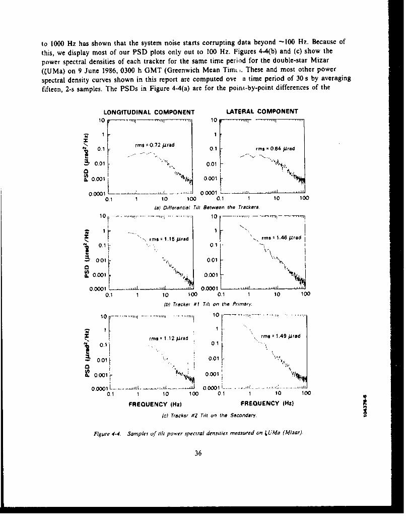
to 1000 Hz has shown that the system noise starts corrupting data beyond -100 Hz. Because of

this, we display most of our PSD plots only out to 100 Hz. Figures 4-4(b) and (c) show the

power spectral densities of each tracker for the same time period for the double-star Mizar

(;UMa) on 9 June 1986, 0300 h GMT (Greenwich Mean Timr,. These and most other power

spectral density curves shown in this report are computed ove a time period of 30 s by averaging

fifteen, 2-s samples. The PSDs in Figure 4-4(a) are for the point-by-point differences of the

LONGITUDINAL COMPONENT LATERAL COMPONENT10 10 r -- Tn,,

"L [ rrns 0.72 M, rad14 0.10 01 rms 0.64 Arad

0.011 - 0.01

tL 0.001 0.001

0 .000. ',•' - - 0 .oo0 1 . . . '" . . .. . . ...I

0.1 1 10 100 0.1 1 10 100

(a) Differential Tilt Between the Trackers10 • -. -.- *-r-.....---' 'i.......: 10 . ...- ,• --. •---

z , , rms 1.15 Atrad 1.. rms: 1.46 Arad

0.1-0.1 -Ooi: 0o1--i\i oo,CL 001 O.C001 I

0.0001 -. _. . .-1[ 0.0001

0.1 1 10 100 0.1 1 10 100

(b) Tracker #1 Tilt on the Primary,

10 i -ml 10 } -- ' - Ii ,

rms: 1.12 lr,,d I rms :1.49 Arad0'. 0 .1 -

""0O-- . . v\-- 0.01 " ... , 0.01 ".

0.0001 L .. .,:. . .... _u 0.0001 i... .. ,. . .. ..... •

0.1 1 10 100 0.1 1 10 100

FREQUENCY (Hz) FREQUENCY (Hz)

(c) Tracker #2 Tilt on the Secondary.

Figure 4.4, Sampler of tilt power spectral densitie. measured on 4UMa (Mizar).

36

rotated tracker signals. This difference is the tilt anisoplanatism spectrum, and its integral overthe frequency domain is the variance of tilt anisoplanatism. Usually, we report the square root ofthe variance, between 0.5 and 100 Hz, and call it rms differential tilt.

4.4.3 Determination of System Noise

The differential tilt shown in Figure 4-4(a) includes tracker system noise which can be calcu-lated and subtracted to give a better estimate of the tilt anisoplanatism. The system noise isapproximated by tracking the primary and secondary stars with both trackers. The differential tiltshould be identically zero for these control cases except for the system noise. Even though thesenoise measurements are made at different times, the system noise should stay the same over shortperiods of time. Assuming that the system noise is statistically independent of the tilt anisoplana-tism, we can subtract the noise PSD directly from the differential tilt PSD. Figure 4-5 shows thenoise power spectral density plots for the same Mizar run as shown on Figure 4-4. Because themeasured noise during the two control measurements is slightly different, as shown by Figure 4-5,we average the two measurements for subtraction. Subtracting this average system noise of Fig-ure 4-5 from the differential tilt of Figure 4-4(a) gives us a somewhat lower value of tilt aniso-planatism, but hardly any difference is detected in the PSDs when the with- and without-noisecurves are overlayed.

4.4.4 Normal vs Flipped Differential Tilt

Since it takes some time ("-5 min) to adjust the boresight with the bias blocks, the normaland flipped measurements are made under different atmospheric conditions and sometimes givequite different results.

Figure 4-6 shows the 2-axis rms tilt anisoplanatism for the double-star measurements undernormal and flipped conditions. The two values are plotted as a function of measurement number.It can be seen that, while many measurements were close to each other, sometimes tilt anisoplan-atism changed considerably during only a few minutes that were required to flip the trackers.Our experience indicated that the change in tilt anisoplanatism was due to atmospheric condi-tions changing, and was not affected by flipping the trackers. Note that in Figure 4-6 no flipmeasurements were made for measurement numbers 28 or greater.

4.5 MONITORING OF ATMOSPHERIC VARIABLES

Tilt anisoplanatism is strongly dependent on the turbulence profile and, in order to be ableto compare theoretical predictions with measurements, it would be desirable to measure theatmospheric structure constant (C2) as a function of altitude. Since it is difficult to measure C2

n ndirectly, we decided to measure something that would be indicative of the turbulence strength athigh and low altitudes. The atmospheric coherence length (r.) and the isoplanatic angle (00) aretwo integrals of the structure function (C2) which weight the structure function with altitude inthe following way (Reference 7):

37

LONGITUDINAL COMPONENT LATERAL COMPONENT10.1 10. - .

rms :0.18 Arad rms :0.17 Arad'. 10-2 10.2.L 10-3 l-o ,

10- J 10.-

0.1 1 10 100 0.1 1 10 100

(a) System Noise Measured with Both Trackers on the Primary Star.

10-1 101[.................1

; rms: 032Arad rms 0.34/.Arad

t "0...-3.. . 10.3I ":"" "

S104~jSa 1024

o o4 i.

0.1 1 10 100 0.1 1 10 100

(b) System Noise Measured with Both Trackers on the Secondary Stat

10 1 10. -

"10.21tirms =0.26 /.rad 0 rms =0.28 AradS10.2 10-2

V '- 1

S104 t, 104 7

o. 10 .5 . .. 1- , • ,• . . . . • 10s l . . ... "51- -.-,•

0.1 1 10 100 01 1 10 100

FREQUENCY (Hz) FREQUENCY (Hz)

1c) Average Differ3ntial Tilt System Noise.

Figure 4-5. Determination of differential tilt system noise on 4 UMa (Mizar). Average noise PSD

for each component is the sum of the two top curves divided by 2.

38

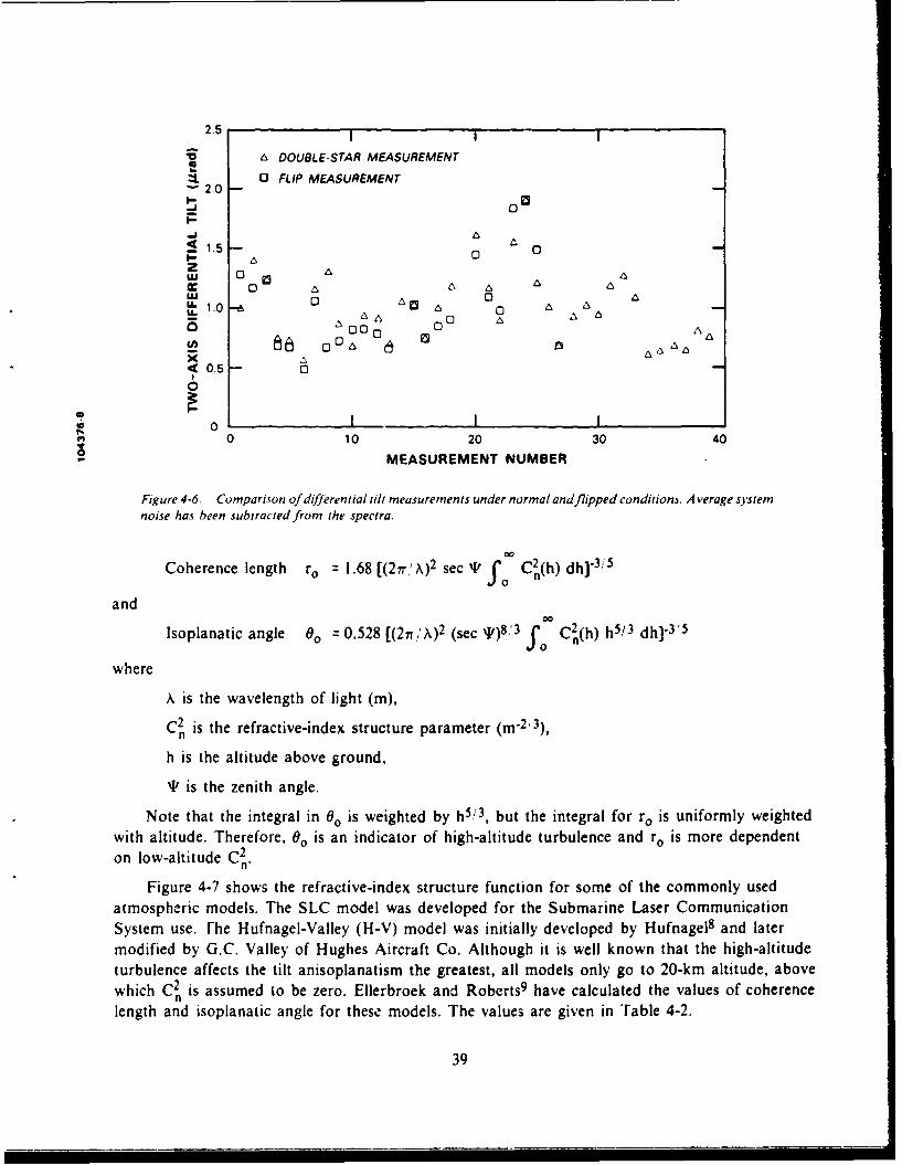
2.5

A DOUBLE-STAR MEASUREMENT

1 2.0 FLIP MEASUREMENT

00I-

A

:5 1.5 0 01.- 0Z

00 0a 0 A" A A Ax A

6 1.0 -.-•6 0 6•.. 6

A 0 0 0 0 A a

40.5 06

"o I I

% 0 10 20 30 40MEASUREMENT NUMBER

Figure 4-6. Comparison of differential tilt measurements under normal andflipped conditiono. Average system

noise has been subtracted from the spectra.

Coherence length ro = 1.68 [( 2 1r'X) 2 sec qI' 3o C2(h) dh]3'i 5

andcc

Isoplanatic angle 00 = 0.528 ((2n,'\)2 (sec 4I')8,'3 3o C2(h) h5/3 dh]-3 '5

where

X is the wavelength of light (m),C2 is the refractive-index structure parameter (m-2 '3),

h is the altitude above ground,

T' is the zenith angle.

Note that the integral in 00 is weighted by h5' 3, but the integral for ro is uniformly weightedwith altitude. Therefore, 00 is an indicator of high-altitude turbulence and r. is more dependenton low-altitude C2

n"

Figure 4-7 shows the refractive-index structure function for some of the commonly usedatmospheric models. The SLC model was developed for the Submarine Laser CommunicationSystem use. rhe Hufnagel-Valley (H-V) model was initially developed by Hufnagel 8 and latermodified by G.C. Valley of Hughes Aircraft Co. Although it is well known that the high-altitudeturbulence affects the tilt anisoplanatism the greatest, all models only go to 20-km altitude, abovewhich C2 is assumed to be zero. Ellerbroek and Roberts 9 have calculated the values of coherencelength and isoplanatic angle for these models. The values are given in Table 4-2.

39

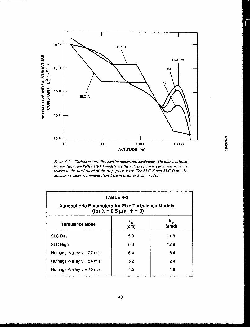
10SLC D

wUH-V 70

• IO• 54

x " 27

? Z 1016

2LITD (m)

I-- 4~-0

U.wj 10"

1010

10 100 1 100 10000

ALTITUDE (in)

Figure4-7 Turbulence profiles usedfor numerical calculations. The numbers listedfor the Hufnagel-Valleley (H- V) models are the values of a free parameter which isrelated to the wind speed of the Iropopause layer. The SLC N and SLC D are theSubmarine Laser Communication System night and day~ models.

TABLE 4-2

Atmospheric Parameters for Five Turbulence Models(for X = 0.5 g.m, P = 0)

Turbulence Model ro 00(cm) (pirod)

SLC Day 5.0 11.8SLC Night 10012.9

Hufnagel-Valley v = 27 mis 6.4 5.4

Hufnagel-Valley v = 54 m's 5.2 2.4

Hufnagel-Valley v = 70 m/s 4.5 1.8

40

We can estimate the atmospheric coherence length from measurements of tilt jitter to a star.The variance of angle-of-arrival jitter due to atmospheric turbulence is related to the coherencediameter by

02 = 0.1675 (Diro)5 / 3 (X; D)2

where

D is the diameter of the telescope aperture (1.2 m for the Firepond telescope), and

X is the wavelength (peak sensitivity of our photomultipliers is at X = 0.35 Am).

While the Firepond measurements are made at 0.35 Mm, we can scale the results to 0.5 ymfor comparison with calculated values given in Table 4-2. The atmospheric coherence length canbe easily calculated from the I-axis tilt a by

r. = 11 0-6 5, where a is in prad rms and ro will be in cm for X = 0.5 Mtm

Figure 4-8 shows the atmospheric coherence length as a function of time of day which wasobtained by converting Polaris tracking data to ro by the above formula. The time is given in

20 1

LOCAL SUNSET LOCAL SUNRISE

16 (o ,o _ ,I i_

I . ,: '..,I

z

1'/ "'

-J

wz 1220

z

0.

o

a~o• GMT HOURS

Figure 4-8. Atmospheric coherence length ro implied from a L"Mi (Polaris) tiltduring five summer nights.

4'

Greenwich Mean Time (GMT) which is 4 h ahead of local daylight savings time in Massachu-setts. Thus, the sunset neutral event should occur slightly after 1200 h GMT, i.e., slightly beforeour measurements.

Loos and Hogge6 suggested that amplitude scintillations measured with an I I-cm-diam. aper-ture provide a good estimate of the isoplanatic angle 00. The instrument which we have built issimilar to the one described by Eaton et al.WO of the Atmospheric Sciences Laboratory (ASL),which has been successfully used at White Sands Missile Range for 00 measurements. Theinstrument measures the percent modulation of the amplitude of the star light. The measuredquantity is the percent modulation as/S, which is related to 00 by

00 K[= n (0 + o2sS2)]-3 5

whereus is the standard deviation of the signal,

S is the average signal amplitude,

K is the calibration constant of the scintillometer (ASL, in Reference 10, has experi-mentally determined that K = 0.9676 .lrad, and the -3/5 exponent should be 0.6387for an Il -cm instrument aperture).

The Firepond instrument has not been calibrated against any other instrument, but appearsto be working well. The values of 00 which are given in this report were derived by use of theASL calibration constants which should be applicable to our instrument. Thus, we used the fol-lowing equation for converting percent modulation to isoplanatic angle:

00 = 0.9676 [in (I + a2i S2)]"0. 6387 for 00 in Mrad for X = 0.5 ym

Figure 4-9 shows the isoplanatic angles determined from the scintillation of Polaris duringthe measurements. An interesting phenomenon, shown in the figure, is the tendency for isopla-natic angle to reach higher values just before dawn. Although our data base is sparse, this per-haps explains why planetary observers have noted best resolution long after midnight towarddawn! More measurements of this effect are needed since it perhaps indicates a time periodwhere beam pointing experiments are better performed.

4.6. TILT ANISOPLANATISM DATA

The data from all the measurements were collected in a data base and plotted in variousforms to get an insight into the trends and nature of tilt anisoplanatism. Here, we show only thetilt anisoplanatism as a function of the atmospheric coherence length and the isoplanatic angle.

4.6.1 Tilt Anisoplanatism vs Atmospheric Coherence Length

Figure 4-10 shows the tilt anisoplanatism data plotted as a function of the atmosphericcoherence length ro. The value of ro was obtained from the total tilt variance of the primary star,

42

8

LOCAL SUNSET LOCAL SUNRISE

6

2 5

2 4

CL.

U, , zx,,5 Ls \ / -j-

.*~. ..... ... .. "

o 20 2 4 6 8 10

GMT HOURS

Figure 4-9. Isoplanatic angle 0,, at the Firepond site daring five summer nights. Obtainedfrom percent amplitude modulation of light from a LIMi (Polaris).

so that the atmospheric coherence length is for the same path and the same time as the tilt anis-oplanatism measurements. Data points are shown for double stars -yDel, 4UMa, and OSer whichhave quite different separations. The scatter of the data points does not appear to give a cleartrend. Even double stars with different separations do riot appear to form different data sets.

4.6.2 Tilt Anisoplanatism vs Isoplanatic Angle

Figure 4-11 shows a plot of tilt anisoplanatism as a function of isoplanatic angle. Here, theoverall trend is somewhat noticeable. As one would expect, the tilt anisoplanatism is much largerfor smaller isoplanatic angles. The isoplanatic angle for this curve was derived from the Polarismeasurements, by adjusting the isoplanatic angle according to the sec T, where I is the zenithangle to the star on which the differential tilt was measured.

In general, this plotting procedure produced no clear trends in these data sets. It was decidedthat the data had to be adjusted according to theoretically predicted formulas to reduce scatter.

43

2.0 I 1

A yDel (48 ,red)

0 WUMe (70 pred)

1.5 0 3 X OSer (708 prad)

~Xo 0

1. o x 3

c 05

W 1.500

2 O

U.

"K X

-6 0 U

a. 1.54 -- x 0Se (18x

' 0

0 0

00_,

3~ 1.0II

0 5 10 15 20

(a) Longitudinal Component.

20

6 'jDel (48 prad)

0 WUMa (70prad)

~.. i~bX OSer (108 prad;IJE

0-j

002 0LU 1.01

wo.X 0C3oX

0

0 5 10 15 20

ATMOSPHERIC COHERENCE LENGTH, ro (cm)

(b) Lateral Component

Figure 4-10. Differential tilt as afunction of atmospheric coherence length. Note that

the data are for three double-star separations but data for each star do not follow aseparate trend.

44

0 2.5 I I 1

a -yDel (48 predl

0 UMa (70 ired)2. 02.0 (X 8Ser (008 iured)

a-

z 00

0 1.5°AI--

2TREND LINE X

1.0 0 a

-3 0 0 oz o 0

I,- 0. 0

0

oI . I I I

0 2 4 6 8 10

(a) Longitudinal Component.

2.51

A y'De/ (48 Aired)

2.0 -0 ZUMa (70 Ai'adJ20 X OSer (708 grad)

15

0.4 1.0 TREND LINE0

00

0 2 4 6 810

ISOPLANATiC ANGLE ADJUSTED TO STAR ELEVATION (prad)

i(bi Lateral Component.

Figure 4-11. Tilt anisoplanatism as a function of isoplanatic angle. Thie trend line was drawnby ey'e to point out the trend that the data appear to follow.

45

6 -yDeI (48 kited)

D0 0 OUa (70 urad)

X OSer (108 jiral)1.5 9

W * 1.0cc1 HUFNAGEL-VALLEY 27

aA a- .- -

2 05 Q0C-L DAY

20

0 -Ie - - - Id

0 50e 100 150 200

200

15 15a-jM

105w x

ccLA.

SLCDA

000101020C057

DOBL-SA SEAAINx ecV pa)11

44

4.7 COMPARISON OF FIREPOND DATA WITH THEORY

While the theory of tilt anisoplanatism is new, several individuals have performed calcula-tions predicting the magnitude of tilt anisoplanatism. We contracted with the Optical SciencesCo. (tOSC) to make specific predictions of differential tilt for the Firepond 1.2-m telescope andnon-nutating quadrant detectors. This report will not describe their theoretical results, but willsimply show the tOSC numerical calculations in comparison with the Firepond measured data.More detailed information on tOSC work can be found in their reports which are referencedherein. B. Ellerbroek has shown mathematically' that a quad detector approximately measuresG-tilt (the aperture averaged gradient of the wavefront) rather than Z-tilt (the best-fit plane tothe measured wavefront). Reference 12 shows that the difference between what a null-trackingquad like ours measures and G-tilt is more than an order-of-magnitude lower than differential tiltunder an interesting range of parameters. Accordingly, all the other tOSC calculations shown inthis report are G-tilt values.

4.7.1 Tilt Anisoplanatism vs Double-Star Separation

When normalizing the tilt anisoplanatism and the double-star separation by the sec 91 func-tions, one obtains the curves of Figure 4-12. The figure also shows computed curves for threeatmospheric models which appear to bracket the measured data. The SLC Day model appears tobe the lower bound of our nighttime measurements. Because tilt anisoplanatism is a high-altitudephenomenon, and because the SLC Day and Night models are the same at high altitudes, theSLC Night model is not shown on the figure but would fall on top of the SLC Day curve. TheHufnagel-Valley models have a free parameter which can be adjusted to provide any strengthturbulence one wishes at high altitudes. For these data, the Hufnagel-Valley 54 model appears tobracket the data on the high side, except for a few anomalous points.

The theoretical computations are made t. ing the atmospheric models described in Sec-tion 4.5. The calculations assumea that the atmospheric structure constant vanishes above 20 kmaltitude. H. Praddaude13 has shown that, when these atmospheric models are used to calculatetilt anisoplanatism, the contribution at 20 km altitude is important. R. Sasiela14 has extcnded themodels to include turbulence above 20 km and has obtained ---25-percent higher values of tiltanisoplanatism than computed by tOSC.

Some data values appear to be anomalous on Figure 4-12. We don't believe this to be ameasurement problem; instead, during these measurements, unusual atmospheric conditions per-sisted. In some cases, the image of the star was very small but danced around with an unusuallylarge magnitude. Other times, the image was quite stationary but its size rapidly pulsated. Weattribute these phenomena to unusual high-altitude atmospheric conditions which are not wellunderstood, but were encountered during our measurements on several occasions.

4.7.2 Tilt Anisoplanatism vs Normalized Separation

So far, we have ploted the tilt anisoplanatism data in various forms and have used theatmospheric models to compute theoretical curves which show that the measured data are reason-able if particular "standard" atmospheric conditions are assumed. During the measurements, we

47

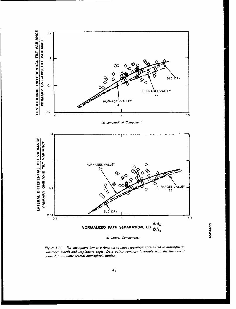
UI 10

Fe .)4x2

> 1

,,4 !J\ ';:0 000"

W' 01I1

LAJ SLC DAYU.

100

4> HUFNAGEL-VALLEY

4 27

0. 54

0 00101 1 10

(a) Longitudinal Component.

10I

z

4 4>

> 1~

U.Ij HUFNAGE L-VLLEY0

00

001j00U;0 01 1 10ELVALE

>D/rIbc <aea Copoen

FiuW 41.Tl nspaaima u iino ahrprto omlzdt topei

computations(b Lsateerlamspei o erls. mpnet

48

also obtained estimates of isoplanatic angle and the atmospheric coherence length, which can beused in predicting the magnitude of tilt anisoplanatism. Glenn Tyler of tOSC has computed thenormalized variance of tilt anisoplanatism for the Firepond telescope as a function of atmo-spheric and system parameters, shown in Figure 4-13, for the SLC and Hufnagel-Valley C2 mod-els (see Reference 9 for details of similar calculations). We also plot the Firepond data on thesame figure, where the vertical axis shows the differential tilt normalized to the total angle-of-arrival tilt, and the horizontal axis shows the value of Q which is defined as follows:

0/00D•"r 0

where

0 is the star separation,

00 is the isoplanatic angle,

D = 1.2 m is the diameter of the telescope aperture,

r. is the atmospheric coherence length.

When the data are normalized in this manner, all models collapse to the same curve forweak turbulence levels or small separations. The values of 00 and r. which were used in Fig-ure 4-13 were measured just before the differential tilt measurements. The isoplanatic angle wasmeasured on Polaris and was adjusted to the double-star's zenith angle.

4.7.3 Longitudinal vs Lateral Component Magnitude

The two components of tilt anisoplanatism are of different magnitude. Comparison of thetheoretical curves of Figures 4-13(a) and (b) and computations by others show that for small sep-arations or weak turbulence conditions the longitudinal component of tilt anisoplanatism in thedirection of the double-star separation is larger than the lateral component in the perpendiculardirection by a factor of square root of 3. For stronger turbulence and larger separation, the ratiobecomes smaller, until at very large separations the two components of tilt anisoplanatismbecome equal. Figure 4-14 shows the ratio of longitudinal component divided by the lateral com-ponent for our measurements; it also shows the range of values which would be expected fromthe actual double-star separation and the measured atmospheric conditions. Clearly, the measuredvalues are lower than theory predicts, indicating stronger turbulence than the models.

4.8 POWER SPECTRAL DENSITY OF THE DIFFERENTIAL TILT

The power spectral density of tilt anisoplanatism is dependent on the cross wind along theline-of-sight, particularly at high altitudes. In order to predict the differential tilt spectrum, thewind velocity has to be known precisely. During our measurements we had no way to measurethe wind-velocity profile. Instead, we relied on the US Weather Service to provide us that infor-mation. Unfortunately, the nearest weather stations to Firepond are in Albany, NY; Portland,ME; and Chatham, MA. The Firepond facility is roughly equidistant from all three stations, asshown on the area map of Figure 4-15.

49

2.01

THEORETI AL PREDICTION O, RATIO FOR OUR VA.UES OF 6irog1- 1.5! (51 D/ro- .s /D< <> 0>

z 0 0 <>88 00 0

I- 1.0 0-J i

0_o osU.

0.5

0 5 10 15 20 25 30

MEASUREMENT NUMBERe,

Figure 4-14. Ratio of longitudinal and lateral components of till anisoplanatism for Firepond data.

50

Rw d PORTLAND ....

C1 00 '(Weni

~* f 1. ~ .~ Portinouth

Y. ....~rý . '* a* . or 'i < _ - FIREPOWIO

Peg.ha~rpionWORCESTERI., ~ -) 0.'3 2* BOSTO

SPIG Fa ScM1I,.1FIELD-kt.

A..

k- I~' CHTA

5'F

Figure 4-16 shows the wind profiles with altitude above the mean sea level for the three sitesfor 10 June 1986 taken at 0 h GMT. As can be seen, the three sites had similar wind profiles,particularly at high altitude. We used the Portland data as being valid at Firepond during thewhole evening of measurements. The actual winds at Firepond were probably quite different atlower altitudes, so the theoretical calculations should not be taken too seriously.

30

.j. 10 -

10 CHATHAM

/ rj PORTLAND

0

0 20 40 60 80 100

WIND SPEED (Knots)

Figure 4-16. Wind profiles at Albany, Portland, and Chatham during the evening of 10 June 1986, 0 h GMT.Wind direction was approximately from the north at all stations. The values for Pot tland were used for pre-dicting power spectral densities at the Firepond site.

52

The Optical Sciences Co. performed calculations valid for the actual elevation angle to thedouble star and detailed wind as measured by the Weather Service at Portland. The wind wasassumed to be in the horizontal direction with zero vertical components. Figure 4-17 shows thecalculated frequency spectra for various atmospheric models. These 2-axis PSD curves are for thedouble-star Mizar with a separation of 70 prad at an elevaticn angle of 730. While agreementbetween the measurements and calculations is quite good, we must point out that the shape ofPSD curves changed substantially from one measurement to the next.

100 1 11111 1 1111111

HUFNAGEL-VALLEY 70 HUFNAGEL-VALLEY 54

101

10-2

~O 10-3

HUFNAGEL-VALLEY 27

0a, 10.4

10-5 .SLC DAY

107

* 01 1 10 100 1000

FREQUENCY (Hz)

Figure 4-17. Power spectral density of total differential tilt of UMa (dashed curve) on the evening of 10 June 1986(02.11:16 GMT) compared with theoretical calculations.

53

Figures 4-18 and 4-19 show some samples of power spectral densities taken during the sameevening. We assume that the winds stayed the same during the whole cvening, so that the differ-cnces in the shape of the PSD curves are due to different atmospheric seeing conditions and per-haps the elevation angles.

Figure 4-18(a) shows the longitudinal and lateral components of the power spectral densityfor reasonably benign conditions. The rms tilt anisoplanatism was well below I Arad. In Fig-ure 4-18(b) we have the power spectral densities for the same star (Mizar) when the tilt aniso-planatism was well above 1.5 ,grad. We note that for the higher tilt anisoplanatism case, the lowfrequencies increase by almost a factor of 10 and also the hump at "-60 Hz which was predictedby the theoretical curves starts appearing.

Figure 4-19 shows the shape of the spectra for three double-star separations. The spectra arequite different for the different separations; however, it is not clear whether the shape changesbecause of the star separation or because of some other condition which has changed. Note thatthe magnitude of the tilt anisoplanatism is quite different for Figures 4--19(a), (b), and (c). Fromthese limited samples and many others thiat were collected at Firepond, one must conclude thatthe shape of the PSD curves can be highly variable. For strong tilt anisoplanatism, most energyis below 20 or 30 Hz and drops off rather quickly. While our system was not able to measure tiltanisoplanatism beyond 100 Hz, the lower-frequency PSD curves appear to indic.-te that the tiltanisoplanatism energy is negligible above 100 Hz.

54

o 100 100

IO_ 10.1

10.2 10Q.2(C4

1'0.z- 10-3.

S 0-4- 10-4

1O-S ........ I 10-601 1 10 100 0.1 1 10 100

(a) 02:11:76 GMT- Longitudinal (Left) and Lateral (Right) Components Are 0.56- and0.53-•rad rms, Respectively. r. 7.2 cm. 8o 4.3 #rad. Elevation- 73'.

10.1 10-1

So10-3

UJ,.L 10 "10.

U~. w 10-'r 101

0.1 1 10 100 0.1 1 10 100

SFREQUENCY (Hz) FREQUENCY (Hz)

(b) 05 55:46 GMT -Longitudinal (Left) and Latera; (Right) Components Are 1.7- and1.4-prad rms, Respectively. ro = 3.b cm, io = 4.5 trad, Elevation = 420.

Figure 4-18. Typical power spectral densities taken during the evening of 10 June 1986on the double-star ýUMa (Mizar).

55

o 100 A 100.

,._j 102., 1.

, .,; . -.,7U V

1o- 10-4ir 10-4.

10-51.

0.1 1 10 100 0.1 1 10 100

(a) "yDel - 48.Mead Separation.

o 100 - . . .. 100

€a. -I • •I- ., I10'

10-100.1

10-2 10-2

Z 103~ 10-3U,, 10.4 t. 1 0.4 ,

0.1 1 10 100 0.1 1 10 100

(b) I4UMa (Mizar) - 70-jsrad Separation.o 100 100

10.1 1010

-tJ•~ Iia) 70- irdSertin

N 102 . 10-2

W 10- 3 : 10.3

O, 10J lO-, lo-.L0. r

10-4 1- n

0o1 1 10 100 .1 1 10 100 cc

FREQUENCY (Hz) FREQUENCY (Hz)

(c) OSer - 108-.rad Separation.

Figure 4-19. Power spectral density for three double-star separations for longitudinal (left)and lateral (right) components during the evening of 10 June 1986.

56

5. CONCLUSIONS

The magnitude of tilt anisoplanatism as a function of angular separation has been measuredwith the Firepond telescope and two precise optical trackers. The precision of the measurementswas demonstrated to be sufficiently fine to measure the relatively small tilt anisoplanatism angles.The major conclusions of these measurements are given in the following paragraphs.

Tilt anisoplanatism is much greater than has been predicted by commonly used SLC models.It is a high-altitude phenomenon which can be modeled appropriately by increasing the freeparameter in the Hufnagel-Valley atmospheric models for the refractive index structure function.

For a star separation of 50 prad, tilt anisoplanatism can typically be between 0.5 and I pradin each axis when using a 1.2-m-diam. telescope aperture. The longitudinal component along thepath separations is slightly larger than the lateral component. That ratio is somewhat lower thanpredicted by theory.

The measured data indicate that it is possible to predict tilt anisoplanatism magnitude fromatmospheric coherence length and the isoplanatic angle. The isoplanatic angle affects the magni-tude of tilt anisoplanatism more than the atmospheric coherence length.

While the shape of the power spectral density of tilt anisoplanatism measured of double starsis extremely variable, most energy lies at lower frequencies (<30 Hz) and is almost negligibleabove 100 Hz.

57

ACKNOWLEDGMENTS

Since many individuals have been involved in the double-star measurements pro-gram, it would be impossible to single out every one who contributed to this work.Here we will recognize the contribution of some, other than the authors, who hadsignificant impact on the project. We would first like to acknowledge the support,encouragement, and review of Leo Sullivan who was particularly instrumental inthe overall system approach and the design and fabrication of the double-starmeasurement hardware. The subject of tilt anisoplanatism has been discussed withmany individuals; among those willing to listen were: H. Praddaude, R. Sasiela,and R. Parenti of Lincoln Laboratory; R. Fugate and R. Cleis of the Air ForceWeapons Laboratory; and G. Tyler, B. Ellerbroek, and D. Fried of the OpticalSciences Company. The Optical Sciences Co. team, under contract to LincolnLaboratory, deserves special recognition for doing most of the numerical calcula-tions which are given in this report and providing us with insight into the tiltanisoplanatism phenomenon. A. Dyer, H. Feinstein, J. Watson, E. Visconti, andM. Mattei participated heavily in the design, construction, and checkout of thedouble-star tracking hardware, and A. Ruscitti was instrumental in accomplishingdata reduction.

59

REFERENCES

I. D.L. Fried, "Anisoplanatism in Adaptive Optics," J. Opt. Soc. Am. 72, 52 (1982).

2. D. Hoffleit, "Seeing," Sky Telescope 9, 57 (1950).

3. J.H. DeWitt, R.H. Hardie, and C.K. Seyfert, "A Seeing Compensator EmployingTelevision Techniques," Sky Telescope 17, 8 (1957).

4. Editors Report, "American Astronomers Re',ort," Sky Telescope 31, 345 (1966).

5. L.J. Sullivan, "Infrared Coherent Radar," CO- Laser Devices and Applications,Proc. SPIE 227, 148 (1980).

6. G.C. Loos and C.B. Hogge, "Turbulence of the Upper Atmosphere and Isoplana-tism," Appl. Opt. 18, 2654 (1979).

7. P. Couteau, Observing Visual Double Stars (MIT Press, Cambridge, MA, 1981).

8. R.E. Hufnagel, "Variations of Atmospheric Turbulence," Digest of TechnicalPapers, Topical Meeting on Optical Propagation Through Turbulence,Optical Society of America, Washington, DC, 1974.

9. B.L. Ellerbroek and P.H. Roberts, "Turbulence-Induced Angular SeparationMeasurement Errors: Expected Values for the SOR-2 Experiment," the Opti-cal Science3 Co., Placentia, CA (December 1984), private communication.

10. F.D. Eaton, W.A. Peterson, J.R. Hines, and G. Fernandez, "Isoplanatic AngleDirect Measurements and Associated Atmospheric Conditions," Appl. Opt. 24,3264 (1985).

II. B.L. Ellerbroek, "The Measurement of Turbulence-Induced Wavefront Tilt Using aNutating Quadrant Detector," the Optical Sciences Co., Placentia, CA, report inpreparation.

12. B.L. Ellerbroek, "Measuring the Apparent Angular Separation of Binary StarsWith a Pair of Quadrant Detectors," the Optical Sciences Co., Placentia, CA,report in preparation.

13. H.C. Praddaude, MIT Lincoln Laboratory, private communication.

14. R.J. Sasiela, MIT Lincoln Laboratory, private communication.

61

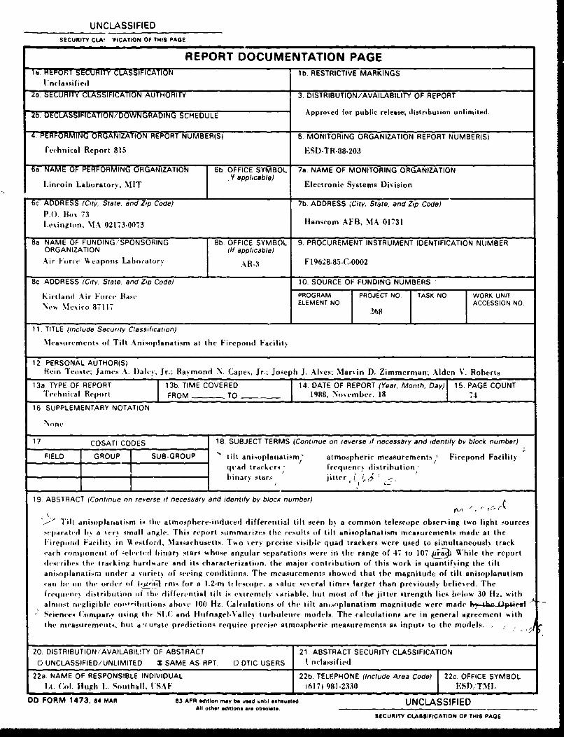
UNCLASSIFIED

SECURITY CLA! 'FICATION OF TH4IS PAGE

REPORT DOCUMENTATION PAGEla lEOTSCRT CASFCTO b. RESTRICTIVE MARKINGS

Unclassi fie d

2a. SECURITIY CLASSIFICATIONY AUTHORITY 3. DISTRIBUTION /AVAILABILITY OF REPORT

Zb ELSIIAINDW AIN SCHEEULE Appro~ed for public release; distribution unlimited.

4. PERFORMING ORGANIZATION4 REPORT NUMBER(S) 5. MONITORING ORGANIZATION REPORT NUMBER(S)

'echnical Report 815 ESI).TR.88.203

6.AMOF PERFORMING ORGANIZATION 6b OFFICE SYMBOL 7a. NAME OF MONITORING ORGANIZATION

inlnLaboratory, MIT ifapial) Electronic Sv stems Div ision

6c. ADDESS (City, State. and Zip Code) 7b. ADDRESS 'City, State. and Zip Code)P.O. Box1 73Lexin~gton, MIA 02173-0073 Hanscom AFB, MIA 017,31

8a NAME OF FUN DING/.SPONSORING I8b. OFFICE SYMBOL 9. PROCUREMENT INSTRUMENT IDENTIFICATION NUMBERORGANIZATION I (If applicable)Air Force \\~ capons Lahoratorv J AR-3 F19628-85-C-0002

8c ADDRESS (City, Stare, and Zip Code) 10. SOURCE OF FUNDING NUMBERS

Kirtland Air Force Ba-c PROGRAM PROJECT No. TASK NO WORK UNITN-Meio87117 ELEMENT NO ACCESSION NO.

11. TITLE (include Security C~assification)

Measurement., of Tilt Anisoplanatism tat the Firepomid Facilitv

12 PERSONAL AUTHOR(S)Rein Teoste. James A. D~ale%. Jr.. Raymond N. Capes, Jr.: Joseph J . Alves, Mariin D. Zimmerman. Alden V. Roberts

13a. TYPE OF REPORT 13b. TIME COVERED 14. DATE OF REPORT (Year, Month, Day 15- PAGE COUNTTechiiical Report 7 1 ROM - TO 1988, November. 18 T 74

16. SUPPLEMENTARY NOTATION

None

17. COSATI CODES 18. SUBJECT TERMS (Continue on reverse if necessary and identity by block number)

FIELD GROUP SUB-GROUP tilt anisoplaitatism' atmospheric measurements IFirepond Facilityq-ad trackers frequency distributionbinar% stars jitter, I I,

19. ABSTRACT (Continue on reverse if necessary and identify by blocg number)

T-1ilt inisoplaiiatism is tilt atmosphere-induced differential tilt seen by a common telescope obseriing two light sourceseparated by a %cry small angle. This report summarizes the results of tilt anisoplanatism measurements made at the

Fireporul Facility in Vestford. MIassachusetts. Twso %ery precise visible quad trackers were used to simnultaneously trackV-ich conmponent of selected binary stars whose angular separations were in the range of 4-7 to 107, 4ýrý hile the reportdescribes the tracking hardware and its characterization, the major contribution of this work is quantifying the tiltaniso)Flanatisn uinder a sariet 'vof geeing conditions. The measurements" showed that the magnitude of tilt anisoplanatismcall be oil the ordler of I 11i'ii1 rmi for a 1.2-in itlescope. a value several times larger than previously believed. Thefrequency dIistrihiition of _IGh differential tilt is estremnel v ariable. but most of Ithe jitter strength 'lies below 30 liz. withalmost ne-gligible co'011rdnatiloiS aboVe 100) HZ. Calculations of the tilt anisoplanatisim magnitude were made 6*-& "-iP4"lI

-Seircince (.omparnv using the SIC and Hlufnagel-Valley. turbuletic models. The calculations are in general agreement wsiththe mcasurt-melits, bilt a - Orat(. prediction,, require precise atmospheric measurements as inputs to the models.

20. DISTRIBUTION,'AVAILABIL!TY OF ABSIRACT 21 ABSTRACT SECURITY CLASSIFICATIONO UNCLASSIFIED/ UNLIMITED 3 SAME AS RPT 0 OTIC USERS ( nclassified

22a. NAME OF RESPONSIBLE INDIVIDUAL 22b. TELEPHONE (Include Area Code) j2 2c OFFICE SYMBOLLt. Col. Hugh L. Southall. I'SAF (6177) 981.2330 1 ESD;TNIL

DD FORM 1473, 84 MAR 83 APR edition masy be used until exhausted UNCLASSIFIEDAll other editions ere obsolete.

SECURITY CLASSIFICATION OF THIS PAGE