DIGITAL SIGNAL PROCESSING [2171003]

Lab Manual 2016

Name:

Enrollment No. :

CONTENTS

Practical

No. Aim

Page

No. Sign.

1(a) w.a.p. to generate sin, cos, sinc and

exponential sequences 3

1(b) w.a.p to generate impulse, unit and ramp

signals. 4

2 w.a.p. for convolution and deconvolution of

given sequence. 5

3 w.a.p. to fold the given sequence. 6

4 w.a.p to find out even and odd function

from the given signal. 7

5(a) w.a.p. to find out transfer function of the

system from zeros and poles. 8

5(b) w.a.p. to find zeros and poles from

Transfer function and plot them on z-

plane.

9

6 w.a.p. to find out z-transform of given

sequences. 11

7 w.a.p. for up sampling and down sampling

of sequence. 12

8 w.a.p. to design IIR filter for analog filter

using butterworth, chebychev1,

chebychev2 and using elliptical.

13

9 Design FIR filter and make use of

(a) Kaiser window

(b) Hamming window

(c) Blackman window

15

10 Design FIR filter using FDA tools. 18

11 To Study Analog to Digital Filter

Transformation. 22

12 To study about TMS320C6713 DSK

processor. 25

Practical No. 1(a)

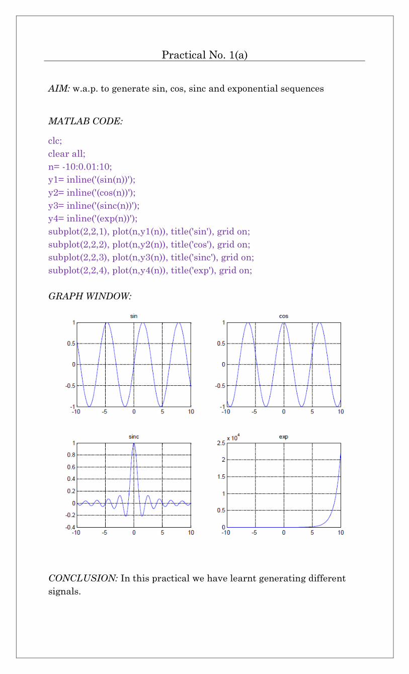
AIM: w.a.p. to generate sin, cos, sinc and exponential sequences

MATLAB CODE:

clc;

clear all;

n= -10:0.01:10;

y1= inline('(sin(n))');

y2= inline('(cos(n))');

y3= inline('(sinc(n))');

y4= inline('(exp(n))');

subplot(2,2,1), plot(n,y1(n)), title('sin'), grid on;

subplot(2,2,2), plot(n,y2(n)), title('cos'), grid on;

subplot(2,2,3), plot(n,y3(n)), title('sinc'), grid on;

subplot(2,2,4), plot(n,y4(n)), title('exp'), grid on;

GRAPH WINDOW:

CONCLUSION: In this practical we have learnt generating different

signals.

Practical No. 1(b)

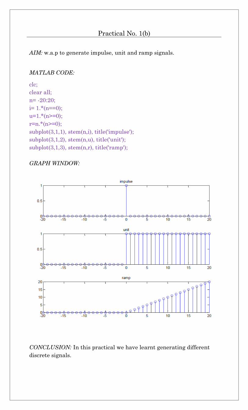
AIM: w.a.p to generate impulse, unit and ramp signals.

MATLAB CODE:

clc;

clear all;

n= -20:20;

i= 1.*(n==0);

u=1.*(n>=0);

r=n.*(n>=0);

subplot(3,1,1), stem(n,i), title('impulse');

subplot(3,1,2), stem(n,u), title('unit');

subplot(3,1,3), stem(n,r), title('ramp');

GRAPH WINDOW:

CONCLUSION: In this practical we have learnt generating different

discrete signals.

Practical No. 2

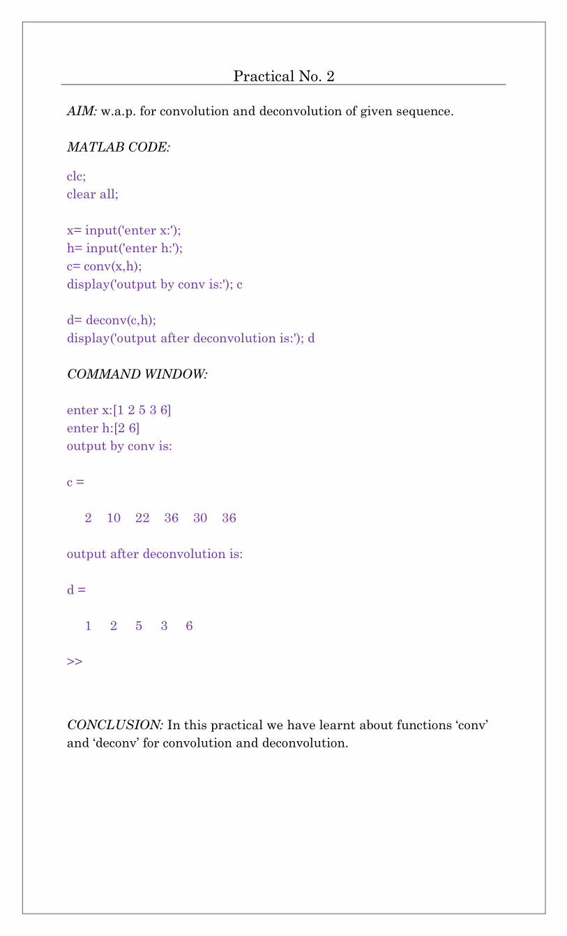
AIM: w.a.p. for convolution and deconvolution of given sequence.

MATLAB CODE:

clc;

clear all;

x= input('enter x:');

h= input('enter h:');

c= conv(x,h);

display('output by conv is:'); c

d= deconv(c,h);

display('output after deconvolution is:'); d

COMMAND WINDOW:

enter x:[1 2 5 3 6]

enter h:[2 6]

output by conv is:

c =

2 10 22 36 30 36

output after deconvolution is:

d =

1 2 5 3 6

>>

CONCLUSION: In this practical we have learnt about functions ‘conv’

and ‘deconv’ for convolution and deconvolution.

Practical No. 3

AIM: w.a.p. to fold the given sequence.

MATLAB CODE:

clc;

clear all;

n= [1 2 3 4 5 6];

a= [4 2 5 6 9 7];

subplot(2,1,1), stem(n,a), grid('on'), title('input');

n1= -fliplr(n);

a1= fliplr(a);

subplot(2,1,2), stem(n1,a1), grid('on'), title('output');

GRAPH WINDOW:

CONCLUSION: In this practical we have learnt about using ‘fliplr’

command for folding of sequences.

Practical No. 4

AIM: w.a.p to find out even and odd function from the given signal.

MATLAB CODE:

clc;

clear all;

n= sym('n');

x= inline('(cos(n))')

display('even function is:')

xe= (x(n)+x(-n))/2

display('odd function is:')

xo= (x(n)-x(-n))/2

COMMAND WINDOW:

x =

Inline function:

x(n) = (cos(n))

even function is:

xe =

cos(n)

odd function is:

xo =

0

>>

CONCLUSION: In this practical we have generated the even and odd

signals of the original signal.

Practical No. 5(a)

AIM: w.a.p. to find out transfer function of the system from zeros and poles.

MATLAB CODE:

clc;

clear all;

z= input('enter zeros as column vector:')

p= input('enter poles as row vector:')

k= input('enter gain in square bracket:')

[num den]=zp2tf(z,p,k);

display('tansfer function is:')

printsys(num,den,'s')

COMMAND WINDOW:

enter zeros as column vector:[1;2]

z =

1

2

enter poles as row vector:[1 3 2]

p =

1 3 2

enter gain in square bracket:[1]

k =

1

tansfer function is:

num/den =

s^2 - 3 s + 2

----------------------

s^3 - 6 s^2 + 11 s - 6

>>

CONCLUSION: In this

practical we have used

command ‘zp2tf’ for getting

transfer function from zeros

and poles.

Practical No. 5(b)

AIM: w.a.p. to find zeros and poles from Transfer function and plot them

on z-plane.

MATLAB CODE:

clc;

clear all

num= input('enter num co-efficient as row vector:');

den= input('enter den co-efficient as row vector:');

[z p k]=tf2zp(num,den)

zplane(num, den)

COMMAND WINDOW:

enter num co-efficient as row vector:[1 2]

enter den co-efficient as row vector:[1 3 2]

z =

-2

p =

-2

-1

k =

1

>>

GRAPH WINDOW:

CONCLUSION: In this practical we have used command ‘tf2zp’ for

getting pole and zeros of transfer function and plotting of them on z-

plane.

Practical No. 6

AIM: w.a.p. to find out z-transform of given sequences.

MATLAB CODE:

clc;

clear all;

n= sym('n');

x= input('enter function in terms of n:')

display('z transform is:')

y= ztrans(x)

COMMAND WINDOW:

enter function in terms of n:2^n

x =

2^n

z transform is:

y =

z/(z - 2)

>>

CONCLUSION: In this practical we have used command ‘ztrans’ for finding

of z-transformation of the sequence.

Practical No. 7

AIM: w.a.p. for up sampling and down sampling of sequence.

MATLAB CODE:

clc;

clear all;

x= input(' enter sequence:')

a= input(' sample factor:')

u= upsample(x,a)

d= downsample(x,a)

COMMAND WINDOW:

enter sequence:[1 7 3 6 4 9]

x =

1 7 3 6 4 9

sample factor:2

a =

2

u =

1 0 7 0 3 0 6 0 4 0 9 0

d =

1 3 4

>>

CONCLUSION: In this practical we have used command ‘upsample’ and

‘downsample’ for up and down sampling of the sequence.

Practical No. 8

AIM: w.a.p. to design IIR filter for analog filter using butterworth,

chebychev1, chebychev2 and using elliptical.

MATLAB CODE:

clc;

clear all;

n = input('enter order of filter:')

f = 2e9;

[zb,pb,kb] = butter(n,2*pi*f,'s');

[bb,ab] = zp2tf(zb,pb,kb);

[hb,wb] = freqs(bb,ab,4096);

[z1,p1,k1] = cheby1(n,3,2*pi*f,'s');

[b1,a1] = zp2tf(z1,p1,k1);

[h1,w1] = freqs(b1,a1,4096);

[z2,p2,k2] = cheby2(n,30,2*pi*f,'s');

[b2,a2] = zp2tf(z2,p2,k2);

[h2,w2] = freqs(b2,a2,4096);

[ze,pe,ke] = ellip(n,3,30,2*pi*f,'s');

[be,ae] = zp2tf(ze,pe,ke);

[he,we] = freqs(be,ae,4096);

plot(wb/(2e9*pi),mag2db(abs(hb)))

hold on

plot(w1/(2e9*pi),mag2db(abs(h1)))

plot(w2/(2e9*pi),mag2db(abs(h2)))

plot(we/(2e9*pi),mag2db(abs(he)))

axis([0 4 -40 5])

grid on

xlabel('Frequency (GHz)')

ylabel('Attenuation (dB)')

legend('butter','cheby1','cheby2','ellip')

COMMAND WINDOW:

enter order of filter:5

n =

5

>>

GRAPH WINDOW:

CONCLUSION: In this practical we have used command ‘butter’, ‘cheby1’,

‘cheby2’ and ‘ellip’ to design IIR filter for analog filter.

Practical No. 9

AIM: Design FIR filter and make use of

(a) Kaiser window

(b) Hamming window

(c) Blackman window

MATLAB CODE:

%FIR FILTER DESIGN

clc;

clear all;

close all;

pr=0.05;sr=0.04;

pf=1500;sf=2000;

f=9000;

wp=2*pf/f;ws=2*sf/f;

%LOW PASS FILTER

N=(-20*log10(sqrt(pr*sr))-13)/(14.6*(sf-pf)/f);

N=ceil(N);

%KAISER WINDOW

beta=5.8;

y=kaiser(N,beta);

b=fir1(N-1,wp,y);

figure(1);

freqz(b,1,256);

title('KAISER WINDOW');

%HAMMING WINDOW

y=hamming(N);

b=fir1(N-1,wp,y);

figure(2);

freqz(b,1,256);

title('HAMMING WINDOW');

%BLACKMAN WINDOW

y=blackman(N);

b=fir1(N-1,wp,y);

figure(3);

freqz(b,1,256);

title('BLACKMAN WINDOW');

GRAPH WINDOW:

CONCLUSION: Here we have designed FIR filter Low pass filter using

Kaiser, hamming and blackman window.

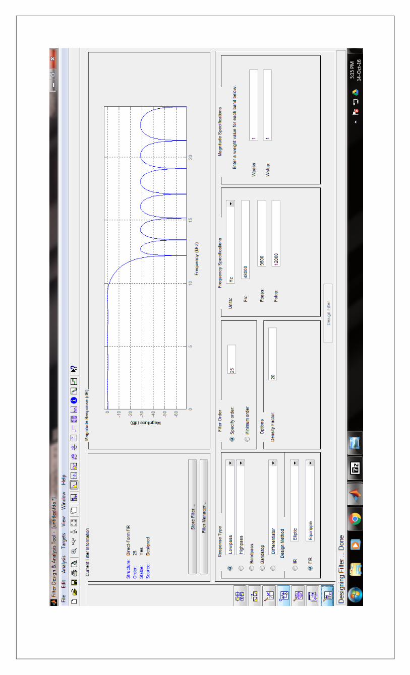
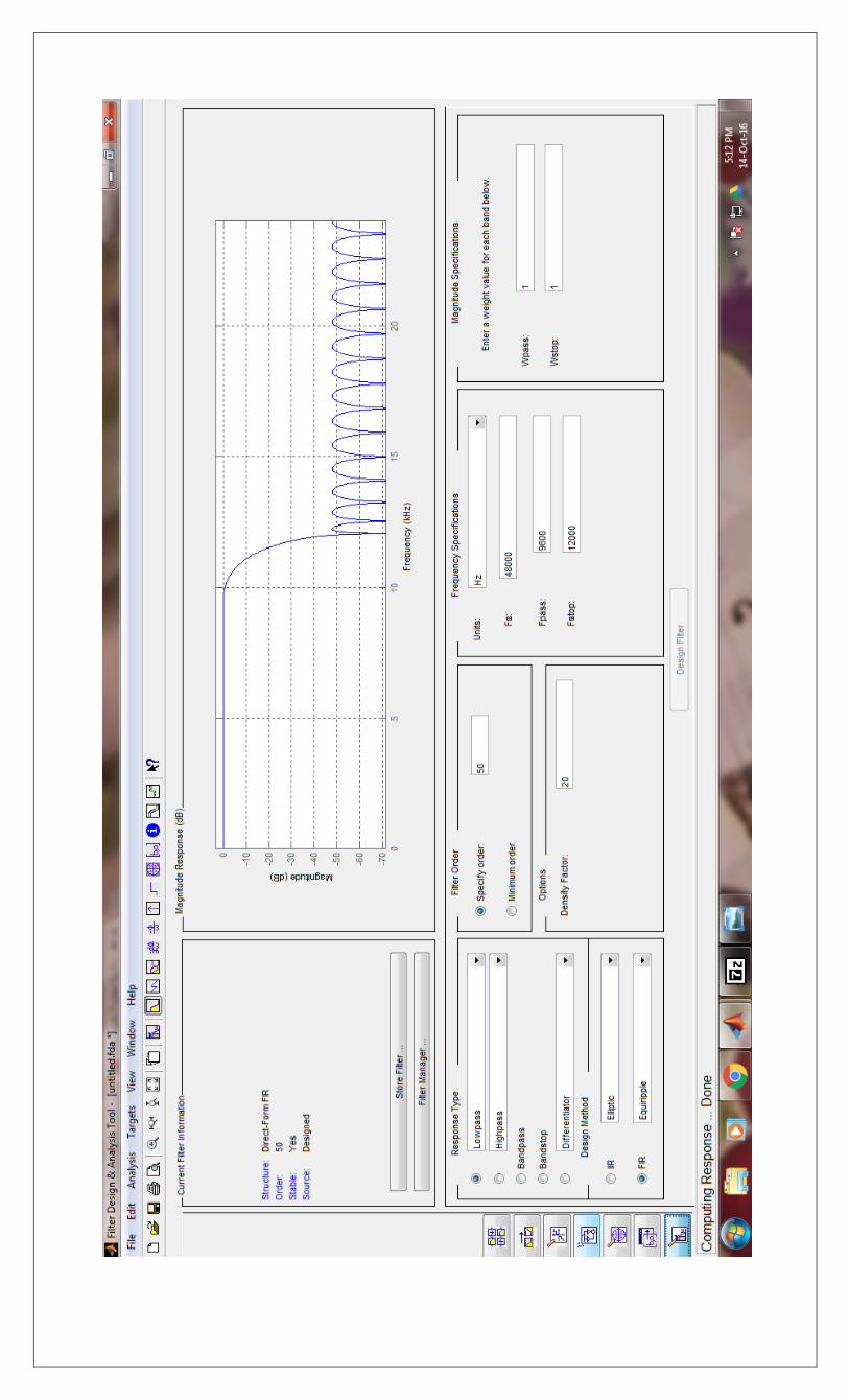
Practical No. 10

AIM: Design FIR filter using FDA tools.

COMMAND WINDOW:

>> fdatool

>>

GRAPH WINDOW:

on next three pages.

CONCLUSION: In this practical we opened fda tool and learnt how to change

filter parameters manually.

EXPERIMENT No.11

AIM: To Study Analog to Digital Filter Transformation. 1) Use impinvar to perform analog to digital filter transformation of

Take T=1s.

2) Use bilinear to perform analog to digital transformation of

Take Ts = 0.1s.

Description:

The classic IIR filter design technique includes the following steps. 1) Find a high pass filter with cutoff frequency of 1 and translate this

prototype filter to the desired band configuration. 2) Transform the filter to the digital domain. 3) Discretize the filter

Matlab functions can be used for filter designing are as below:

1) Impinvar [by, az] = impinvar (b, a, fs) creates a digital filter with numerator and denominator coefficients bz and az, respectively, whose impulse response is equal to the impulse response of the analog filter with coefficients b and a, scaled by 1/fs. If we leave out the argument fs, or specify fs as the empty vector [], it takes the default value of 1 Hz.

2) Bilinear -[numd,dend] = bilinear(num,den,fs) converts an s-domain transfer function given by num and den to a discrete equivalent. Row vectors num and den specify the coefficients of the numerator and denominator, respectively, in descending powers of s. fs is the sampling frequency in hertz. Bilinear returns the discrete equivalent in row vectors numd and dend in descending powers of z (ascending powers of z-1).

Answer:

1) z = [1 0.2];

p = [1 0.4 9.04];

[num den]= impinvar(z,p,1);

sys= filt(num,den,1)

ffplot(sys)

Output:

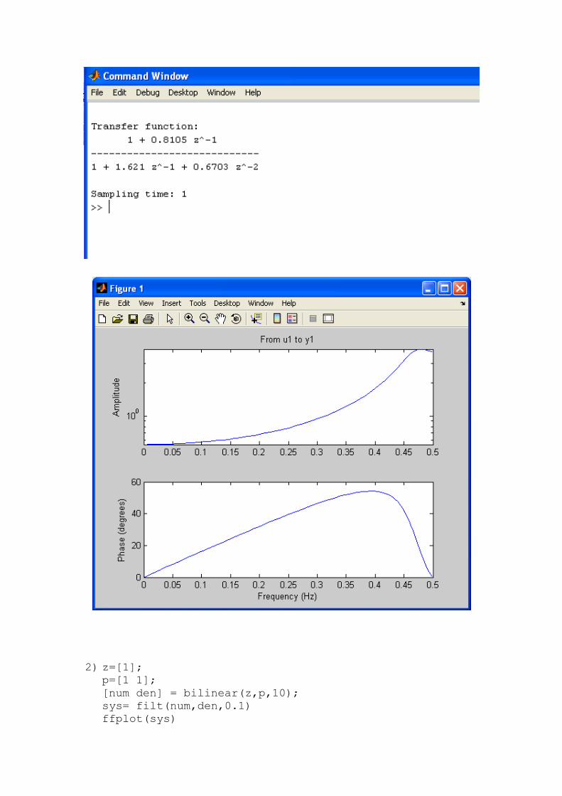
2) z=[1]; p=[1 1];

[num den] = bilinear(z,p,10);

sys= filt(num,den,0.1)

ffplot(sys)

Output

EXPERIMENT 12

Aim: To study about TMS320C6713 DSK processor.

Package Contents

The C6713. DSK builds on TI’s industry-leading line of low cost, easy-to-use DSP Starter Kit (DSK) development boards. The high-performance board features the TMS320C6713 floating-point DSP. Capable of performing 1350 million floating-point operations per second (MFLOPS), the C6713 DSP makes the C6713 DSK the most powerful DSK development board.

The DSK is USB port interfaced platform that allows to efficiently develop and test applications for the C6713. The DSK consists of a C6713-based printed circuit board that will serve as a hardware reference design for TI.s customers. products. With extensive host PC and target DSP software support, including bundled TI tools, the DSK provides ease-of-use and capabilities that are attractive to DSP engineers.

The C6713 DSK has a TMS320C6713 DSP onboard that allows full-speed verification of

code with Code Composer Studio. The C6713 DSK provides:

A USB Interface

SDRAM and ROM

An analog interface circuit for Data conversion (AIC)

An I/O port

Embedded JTAG emulation support

The C6713 DSK includes a stereo codec. This analog interface circuit (AIC) has the

following characteristics:

High-Performance Stereo Codec

90-dB SNR Multibit Sigma-Delta ADC (A-weighted at 48 kHz)

100-dB SNR Multibit Sigma-Delta DAC (A-weighted at 48 kHz)

1.42 V . 3.6 V Core Digital Supply: Compatible With TI C54x DSP Core Voltages

2.7 V . 3.6 V Buffer and Analog Supply: Compatible Both TI C54x DSP Buffer Voltages

8-kHz . 96-kHz Sampling-Frequency Support

Software Control Via TI McBSP-Compatible Multiprotocol Serial Port

I 2 C-Compatible and SPI-Compatible Serial-Port Protocols

Glueless Interface to TI McBSPs

Audio-Data Input/Output Via TI McBSP-Compatible Programmable Audio Interface

I 2 S-Compatible Interface Requiring Only One McBSP for both ADC and DAC

Standard I 2 S, MSB, or LSB Justified-Data Transfers

16/20/24/32-Bit Word Lengths

The C6713DSK has the following features:

The 6713 DSK is a low-cost standalone development platform that enables customers to evaluate and develop applications for the TI C67XX DSP family. The DSK also serves as a hardware reference design for the TMS320C6713 DSP. Schematics, logic equations and application notes are available to ease hardware development and reduce time to market.

The DSK uses the 32-bit EMIF for the SDRAM (CE0) and daughtercard expansion interface (CE2 and CE3). The Flash is attached to CE1 of the EMIF in 8-bit mode.

An on-board AIC23 codec allows the DSP to transmit and receive analog signals.

McBSP0 is used for the codec control interface and McBSP1 is used for data. Analog audio I/O is done through four 3.5mm audio jacks that correspond to microphone input, line input, line output and headphone output. The codec can select the microphone or the line input as the active input. The analog output is driven to both the line out (fixed gain) and headphone (adjustable gain) connectors.

A programmable logic device called a CPLD is used to implement glue logic that ties the board components together. The CPLD has a register based user interface that lets the user configure the board by reading and writing to the CPLD registers.

TMS320C6713 DSP Features:

Highest-Performance Floating-Point Digital Signal Processor (DSP):

Eight 32-Bit Instructions/Cycle

32/64-Bit Data Word

300-, 225-, 200-MHz (GDP), and 225-, 200-, 167-MHz (PYP) Clock rates 3.3-, 4.4-, 5-, 6-Instruction Cycle Times

2400/1800, 1800/1350, 1600/1200, and 1336/1000 MIPS /MFLOPS

Rich Peripheral Set, Optimized for Audio

Highly Optimized C/C++ Compiler

Extended Temperature Devices Available

Advanced Very Long Instruction Word (VLIW) TMS320C67x. DSP Core

Eight Independent Functional Units:

Two ALUs (Fixed-Point)

Four ALUs (Floating- and Fixed-Point)

Two Multipliers (Floating- and Fixed-Point)

Load-Store Architecture With 32 32-Bit General-Purpose Registers

Instruction Packing Reduces Code Size

All Instructions Conditional

Instruction Set Features

Native Instructions for IEEE 754

Single- and Double-Precision

Byte-Addressable (8-, 16-, 32-Bit Data)

8-Bit Overflow Protection

Saturation; Bit-Field Extract, Set, Clear; Bit-Counting; Normalization

L1/L2 Memory Architecture

4K-Byte L1P Program Cache (Direct-Mapped)

4K-Byte L1D Data Cache (2-Way)

256K-Byte L2 Memory Total: 64K-Byte L2 Unified Cache/Mapped RAM, and 192KByte additional L2 Mapped RAM

Device Configuration

Boot Mode: HPI, 8-, 16-, 32-Bit ROM Boot

Endianness: Little Endian, Big Endian

32-Bit External Memory Interface (EMIF)

Glueless Interface to SRAM, EPROM, Flash, SBSRAM, and SDRAM

512M-Byte Total Addressable External Memory Space

Enhanced Direct-Memory-Access (EDMA) Controller (16 Independent channels)

16-Bit Host-Port Interface (HPI)

Two Multichannel Audio Serial Ports (McASPs)

Two Independent Clock Zones Each (1 TX and 1 RX)

Eight Serial Data Pins Per Port:

Individually Assignable to any of the Clock Zones

Each Clock Zone Includes:

Programmable Clock Generator

Programmable Frame Sync Generator

TDM Streams From 2-32 Time Slots

Support for Slot Size:

8, 12, 16, 20, 24, 28, 32 Bits

Data Formatter for Bit Manipulation

Wide Variety of I2S and Similar Bit Stream FormatsIntegrated Digital

Audio Interface Transmitter (DIT) Supports:

S/PDIF, IEC60958-1, AES-3, CP-430 Formats

Up to 16 transmit pins

Enhanced Channel Status/User Data

Extensive Error Checking and Recovery

Two Inter-Integrated Circuit Bus (I2C Bus.) Multi-Master and Slave Interfaces

Two Multichannel Buffered Serial Ports:

Serial-Peripheral-Interface (SPI)

High-Speed TDM Interface

AC97 Interface

Two 32-Bit General-Purpose Timers

Dedicated GPIO Module With 16 pins (External Interrupt Capable)

Flexible Phase-Locked-Loop (PLL) Based Clock Generator Module

IEEE-1149.1 (JTAG ) Boundary-Scan-Compatible

Package Options:

208-Pin PowerPAD. Plastic (Low-Profile) Quad Flatpack (PYP)

272-BGA Packages (GDP and ZDP)

0.13-µm/6-Level Copper Metal Process

CMOS Technology

3.3-V I/Os, 1.2 -V Internal (GDP & PYP)

3.3-V I/Os, 1.4-V Internal (GDP)(300 MHz only)

Procedure to work on Code Composer Studio

1. To create a New Project

Project New (SUM.pjt)

2. To Create a Source file

File New

3. To Add Source files to Project

Project Add files to Project sum.c

4. To Add rts6700.lib file & hello.cmd:

Project Add files to Project rts6700.lib

Path: c:\CCStudio\c6000\cgtools\lib\rts6700.lib

Note: Select Object & Library in(*.o,*.l) in Type of files

Project Add files to Project hello.cmd

Path: c:\ti\tutorial\dsk6713\hello1\hello.cmd

Note: Select Linker Command file(*.cmd) in Type of files

5. To Compile:

Project Compile File

6. To build or Link:

Project build,

Which will create the final executable (.out) file.(Eg. sum.out).

7. Procedure to Load and Run program:

Load program to DSK:

File Load program sum. out

8. To execute project:

Debug Run.

Program:

‘C’ Program to Implement Impulse response:

#include <stdio.h>

#define Order 2

#define Len 10

float y[Len]={0,0,0},sum;

main()

{

int j,k;

float a[Order+1]={0.1311, 0.2622, 0.1311};

float b[Order+1]={1, -0.7478, 0.2722};

for(j=0;j<Len;j++)

{

sum=0;

for(k=1;k<=Order;k++)

{

if((j-k)>=0)

sum=sum+(b[k]*y[j-k]);

}

if(j<=Order)

{

y[j]=a[j]-sum;

}

else

{

y[j]=-sum;

}

printf("Respose[%d] = %f\n",j,y[j]);

}

}

‘C‘ Program to Implement Difference Equation

#include <stdio.h>

#include<math.h>

#define FREQ 400

float y[3]={0,0,0};

float x[3]={0,0,0};

float z[128],m[128],n[128],p[128];

main()

{

int i=0,j;

float a[3]={ 0.072231,0.144462,0.072231};

float b[3]={ 1.000000,-1.109229,0.398152};

for(i=0;i<128;i++)

{

m[i]=sin(2*3.14*FREQ*i/24000);

}

for(j=0;j<128;j++)

{

x[0]=m[j];

y[0] = (a[0] *x[0]) +(a[1]* x[1] ) +(x[2]*a[2]) - (y[1]*b[1])-

(y[2]*b[2]);

z[j]=y[0];

y[2]=y[1];

y[1]=y[0];

x[2]=x[1];

x[1] = x[0];}