Drivers of variability in Euphausiid species abundance throughout

Drivers of variability in Euphausiidspecies abundance throughout thePacific Ocean

TOM B. LETESSIER *, MARTIN J. COX AND ANDREWS S. BRIERLEY

PELAGIC ECOLOGY RESEARCH GROUP, SCOTTISH OCEANS INSTITUTE, UNIVERSITY OF ST ANDREWS, ST ANDREWS, FIFE, KY16 8LB, UK

*CORRESPONDING AUTHOR: [email protected]

Received January 28, 2011; accepted in principle March 11, 2011; accepted for publication March 28, 2011

Corresponding editor: Mark J. Gibbons

Using a generalized additive model, we assessed the influence of a suite ofphysical, chemical and biological variables upon euphausiid species abundancethroughout the Pacific. We found that the main drivers of species abundance, inorder of decreasing importance, were sea surface temperature (explaining 29.53%of species variability), salinity (20.29%), longitude (215.01%, species abundancedecreased from West to East), distance to coast (10.99%) and dissolved silicate con-centration (9.03%). We discuss the influence of these variables within the contextof the known ecology and biology of euphausiids. With reference to a previouslypublished model in the Atlantic, we compare the practical differences in theAtlantic and Pacific Ocean. Using projected environmental change from theIPCC A1B climate scenario, we make predictions of future species abundancechanges in the Pacific and Atlantic. Our model suggests that species abundance inboth oceans between latitudes 308 and 608 (both N and S) will increase due to thetemperature rise predicted over the next 200 years, whereas at low latitudesresponses are likely to differ between the oceans, with little change predicted forthe Atlantic, but species depletion predicted for the Pacific.

KEYWORDS: Pacific; species abundance; Euphausiids; longitude; silicate; seasurface temperature; generalized additive model; climate change

I N T RO D U C T I O N

Euphausiids are an important component of the pelagicrealm. They occupy a key position in marine foodwebs.Many species graze directly on phytoplankton andprovide a food source for a range of predators includingbirds, seals, baleen whales and many commerciallyimportant fish species (Verity et al., 2002). Euphausiidsundertake pronounced diel vertical migration, and haveinfluence outside the photic zone, transporting surface-fixed carbon beneath the thermocline and beyond(Schnack-Schiel and Isla, 2005; Tarling and Johnson,2006; Clarke and Tyler, 2008). Understanding the

drivers of euphausiid diversity on a variety of scales istherefore important for several reasons, such as for thepurpose of ecosystem-based management of fisheriesand marine conservation.

The Pacific Ocean is the world’s largest, and coversroughly 32% of the Earth’s surface (Barkley, 1968). Thebathymetry is complex, more so than in the Atlantic,with the basin containing many deep trenches, seamountsand submerged and semi-submerged volcanic islands.The bathymetry of the southern Pacific is dominated bythe presence of oceanic ridges, which can best bedescribed as underwater mountain chains that are offset

doi:10.1093/plankt/fbr033, available online at www.plankt.oxfordjournals.org

# The Author 2011. Published by Oxford University Press. All rights reserved. For permissions, please email: [email protected]

JOURNAL OF PLANKTON RESEARCH j VOLUME 0 j NUMBER 0 j PAGES 1–16 j 2011 JPR Advance Access published April 29, 2011 at U

niversity of St A

ndrews on M

ay 3, 2011plankt.oxfordjournals.org

Dow

nloaded from

http://plankt.oxfordjournals.org/

by several fracture zones. Several studies have investigatedeuphausiid distribution in the Pacific (Brinton, 1962;Murase et al., 2009) and have investigated euphausiid bio-geography on a meso- (20–200 km) and basin-scale(Lindley, 1977; Gibbons, 1997; Letessier et al., 2009 in theAtlantic; and Trathan et al., 1993 in the SouthernOcean), but there is a gap in our knowledge with respectto basin-scale processes in the Pacific Ocean.

The most striking global pattern in species abun-dance across all marine taxa is a latitudinal decrease inspecies abundance from low latitudes to high latitudes(Fuhrman et al., 2008), a pattern that is most readilydescribed as a polynomial function of sea surface temp-erature (Rutherford et al. 1999). This trend has beenexplained by the species-energy hypothesis (Hustonet al. 2003; Cardillo et al. 2005; Clarke and Gaston,2006), the species-area hypothesis (Currie et al., 2004),the potential energy hypothesis (Jetz et al., 2009) and thehistorical perturbation hypothesis (Stevens, 2006).Tittensor et al. (2010) conducted a global analysis ofmultiple marine taxa, and concluded that thespecies-energy hypothesis (or kinetic energy hypothesis,i.e. high temperature supports higher metabolic ratesand promotes speciation) is best supported.

Marine species abundance has been associated withsea surface temperatures and other variables, such as dis-solved silicate concentration (Roy, 2008) and riveroutputs (Rutherford et al., 1999), but many taxa, includ-ing euphausiids, deviate from the high temperature/diversity trends, and show increasing species numbers atintermediate latitudes (Gibbons, 1997; Rutherford et al.,1999; Letessier et al., 2009). This has been attributed tothe increase in pelagic niches in mid-latitudes, associatedwith the thermal structure of the surface layer(Rutherford et al., 1999) and, in the Atlantic, the depth ofthe mixed layer (deepening of the mixed layerdepth serves to decrease the number of species, Letessieret al., 2009).

The overall picture of pelagic diversity variability iscomplex and includes poorly understood relationships(such as the effect of mid-ocean ridges and seamounts,see Pitcher, 2008). Moreover, global marine data setsfor non-commercial species abundance are rare, andwhere these data sets exist they are of low resolution(either spatially or temporally). Quantitative, long-termdata are virtually non-existent and are by and largelimited to the Continuous Plankton Recorder Surveys inthe North Atlantic and North Sea.

Here, we used a generalized additive statistical mod-elling approach to examine patterns and drivers ofeuphausiid species abundance in the Pacific Ocean inrelation to a suite of environmental and physicalvariables.

We have previously conducted a similar exercise forthe Atlantic Ocean (Letessier et al., 2009) that has pro-vided useful insight into pelagic processes in that basin.

Our second aim was to compare the Pacific modelwith the previously published model for the Atlanticand, so doing, to gain insight into similarities and differ-ences between planktic processes of two oceans.

Thirdly, we sought to model future species abun-dance in both the Atlantic and the Pacific in thecontext of projected environmental conditions in thenext 200 years, and hence to examine the resilience ofthe two oceans to anthropogenic climate change.

M E T H O D

Grid design

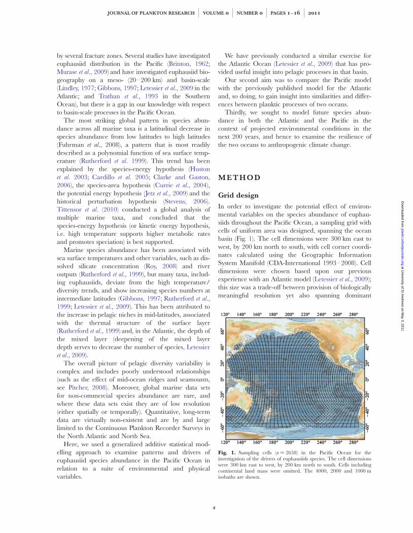
In order to investigate the potential effect of environ-mental variables on the species abundance of euphau-siids throughout the Pacific Ocean, a sampling grid withcells of uniform area was designed, spanning the oceanbasin (Fig. 1). The cell dimensions were 300 km east towest, by 200 km north to south, with cell corner coordi-nates calculated using the Geographic InformationSystem Manifold (CDA-International 1993–2008). Celldimensions were chosen based upon our previousexperience with an Atlantic model (Letessier et al., 2009);this size was a trade-off between provision of biologicallymeaningful resolution yet also spanning dominant

Fig. 1. Sampling cells (n ¼ 2658) in the Pacific Ocean for theinvestigation of the drivers of euphausiids species. The cell dimensionswere 300 km east to west, by 200 km north to south. Cells includingcontinental land mass were omitted. The 4000, 2000 and 1000 misobaths are shown.

JOURNAL OF PLANKTON RESEARCH j VOLUME 0 j NUMBER 0 j PAGES 1–16 j 2011

2

at University of S

t Andrew

s on May 3, 2011

plankt.oxfordjournals.orgD

ownloaded from


underwater features, such as mid-ocean ridges and frac-ture zones. The sampling grid extended between lati-tudes of 618N to 618S and longitudes of 119.088E to70.948W. Continental coastal cells that included majorlandmasses (including Japan and New Zealand) wereomitted, leaving a grid of 3051 cells. The final gridincluded only 11 cells deemed to be ‘on-shelf ’ (averagesea-bed depth ,500 m).

Euphausiid species abundance

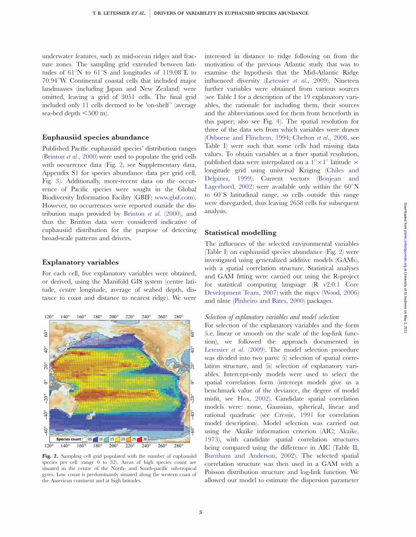
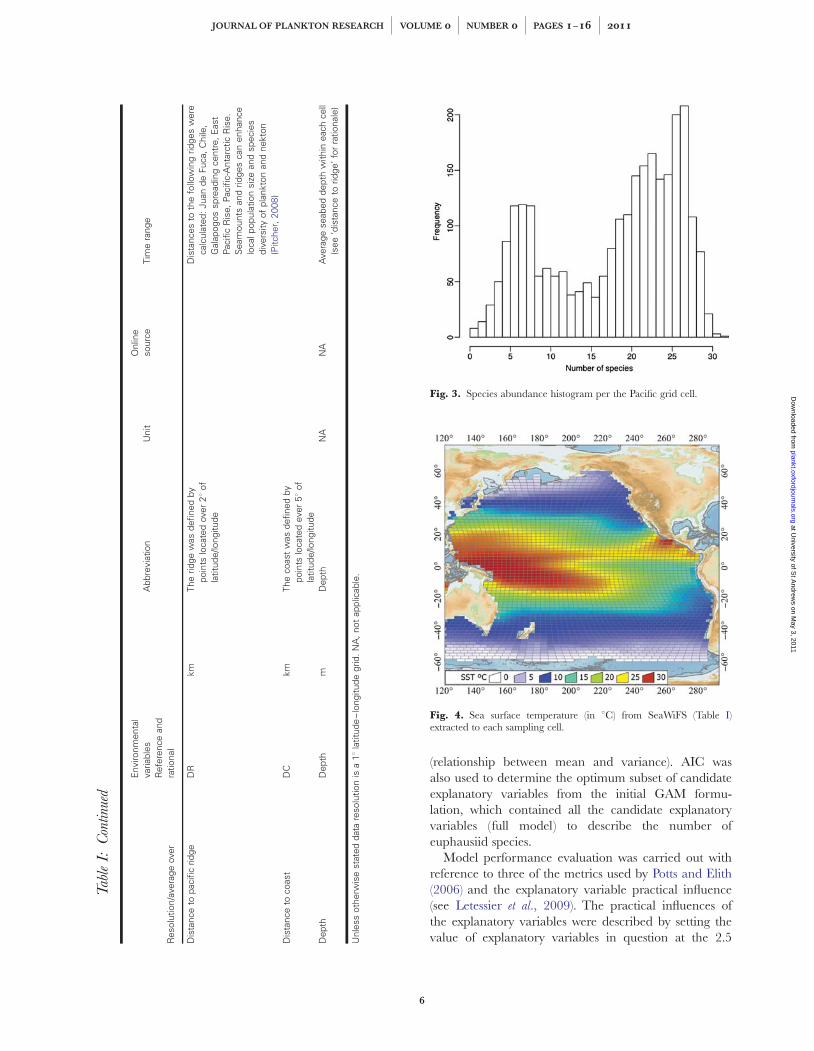
Published Pacific euphausiid species’ distribution ranges(Brinton et al., 2000) were used to populate the grid cellswith occurrence data (Fig. 2, see Supplementary data,Appendix S1 for species abundance data per grid cell,Fig. 3). Additionally, more-recent data on the occur-rence of Pacific species were sought in the GlobalBiodiversity Information Facility (GBIF; www.gbif.com).However, no occurrences were reported outside the dis-tribution maps provided by Brinton et al. (2000), andthus the Brinton data were considered indicative ofeuphausiid distribution for the purpose of detectingbroad-scale patterns and drivers.

Explanatory variables

For each cell, five explanatory variables were obtained,or derived, using the Manifold GIS system (centre lati-tude, centre longitude, average of seabed depth, dis-tance to coast and distance to nearest ridge). We were

interested in distance to ridge following on from themotivation of the previous Atlantic study that was toexamine the hypothesis that the Mid-Atlantic Ridgeinfluenced diversity (Letessier et al., 2009). Nineteenfurther variables were obtained from various sources(see Table I for a description of the 19 explanatory vari-ables, the rationale for including them, their sourcesand the abbreviations used for them from henceforth inthis paper; also see Fig. 4). The spatial resolution forthree of the data sets from which variables were drawn(Osborne and Flinchem, 1994; Chelton et al., 2008, seeTable I) were such that some cells had missing datavalues. To obtain variables at a finer spatial resolution,published data were interpolated on a 18�18 latitude �longitude grid using universal Kriging (Chiles andDelpiner, 1999). Current vectors (Bonjean andLagerhoed, 2002) were available only within the 608Nto 608S latitudinal range, so cells outside this rangewere disregarded, thus leaving 2658 cells for subsequentanalysis.

Statistical modelling

The influences of the selected environmental variables(Table I) on euphausiid species abundance (Fig. 2) wereinvestigated using generalized additive models (GAMs),with a spatial correlation structure. Statistical analysesand GAM fitting were carried out using the R-projectfor statistical computing language (R v2.0.1 CoreDevelopment Team, 2007) with the mgcv (Wood, 2006)and nlme (Pinheiro and Bates, 2000) packages.

Selection of explanatory variables and model selectionFor selection of the explanatory variables and the form(i.e. linear or smooth on the scale of the log-link func-tion), we followed the approach documented inLetessier et al. (2009). The model selection procedurewas divided into two parts: (i) selection of spatial corre-lation structure, and (ii) selection of explanatory vari-ables. Intercept-only models were used to select thespatial correlation form (intercept models give us abenchmark value of the deviance, the degree of modelmisfit, see Hox, 2002). Candidate spatial correlationmodels were: none, Gaussian, spherical, linear andrational quadratic (see Cressie, 1991 for correlationmodel description). Model selection was carried outusing the Akaike information criterion (AIC; Akaike,1973), with candidate spatial correlation structuresbeing compared using the difference in AIC (Table II,Burnham and Anderson, 2002). The selected spatialcorrelation structure was then used in a GAM with aPoisson distribution structure and log-link function. Weallowed our model to estimate the dispersion parameter

Fig. 2. Sampling cell grid populated with the number of euphausiidspecies per cell (range 0 to 32). Areas of high species count aresituated in the centre of the North- and South-pacific sub-tropicalgyres. Low count is predominantly situated along the western coast ofthe American continent and at high latitudes.

T. B. LETESSIER ET AL. j DRIVERS OF VARIABILITY IN EUPHAUSIID SPECIES ABUNDANCE

3

at University of S

t Andrew

s on May 3, 2011


ownloaded from

http://odf.ucsd.edu/joa/




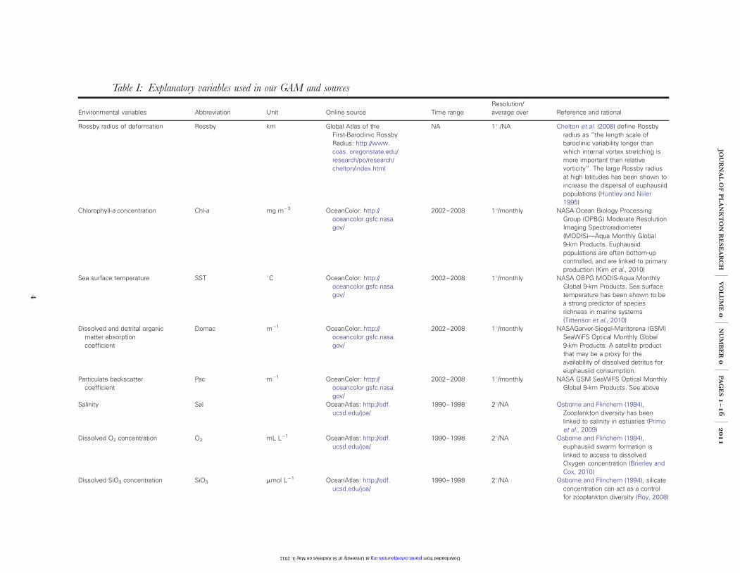
Table I: Explanatory variables used in our GAM and sources

Environmental variables Abbreviation Unit Online source Time rangeResolution/average over Reference and rational

Rossby radius of deformation Rossby km Global Atlas of theFirst-Baroclinic RossbyRadius: http://www.coas. oregonstate.edu/research/po/research/chelton/index.html

NA 18 /NA Chelton et al. (2008) define Rossbyradius as “the length scale ofbaroclinic variability longer thanwhich internal vortex stretching ismore important than relativevorticity”. The large Rossby radiusat high latitudes has been shown toincrease the dispersal of euphausiidpopulations (Huntley and Niiler1995)

Chlorophyll-a concentration Chl-a mg m23 OceanColor: http://oceancolor.gsfc.nasa.gov/

2002–2008 18/monthly NASA Ocean Biology ProcessingGroup (OPBG) Moderate ResolutionImaging Spectroradiometer(MODIS)—Aqua Monthly Global9-km Products. Euphausiidpopulations are often bottom-upcontrolled, and are linked to primaryproduction (Kim et al., 2010)

Sea surface temperature SST 8C OceanColor: http://oceancolor.gsfc.nasa.gov/

2002–2008 18/monthly NASA OBPG MODIS-Aqua MonthlyGlobal 9-km Products. Sea surfacetemperature has been shown to bea strong predictor of speciesrichness in marine systems(Tittensor et al., 2010)

Dissolved and detrital organicmatter absorptioncoefficient

Domac m21 OceanColor: http://oceancolor.gsfc.nasa.gov/

2002–2008 18/monthly NASAGarver-Siegel-Maritorena (GSM)SeaWiFS Optical Monthly Global9-km Products. A satellite productthat may be a proxy for theavailability of dissolved detritus foreuphausiid consumption.

Particulate backscattercoefficient

Pac m21 OceanColor: http://oceancolor.gsfc.nasa.gov/

2002–2008 18/monthly NASA GSM SeaWiFS Optical MonthlyGlobal 9-km Products. See above

Salinity Sal OceanAtlas: http://odf.ucsd.edu/joa/

1990–1998 28/NA Osborne and Flinchem (1994),Zooplankton diversity has beenlinked to salinity in estuaries (Primoet al., 2009)

Dissolved O2 concentration O2 mL L21 OceanAtlas: http://odf.ucsd.edu/joa/

1990–1998 28/NA Osborne and Flinchem (1994),euphausiid swarm formation islinked to access to dissolvedOxygen concentration (Brierley andCox, 2010)

Dissolved SiO3 concentration SiO3 mmol L21 OceanAtlas: http://odf.ucsd.edu/joa/

1990–1998 28/NA Osborne and Flinchem (1994), silicateconcentration can act as a controlfor zooplankton diversity (Roy, 2008)

JOU

RN

AL

OF

PL

AN

KT

ON

RE

SE

AR

CHj

VO

LU

ME0j

NU

MB

ER0j

PA

GE

S1

–16j

2011

4

at University of St Andrews on May 3, 2011 plankt.oxfordjournals.org Downloaded from

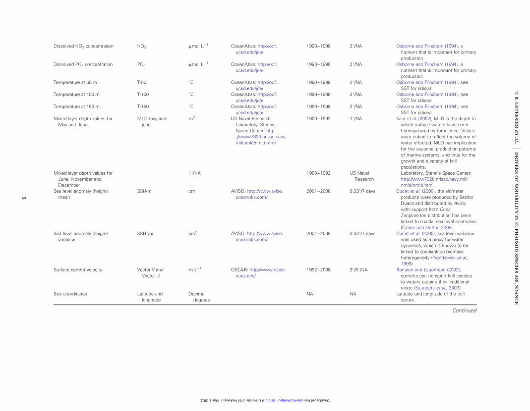
http://www.coas.oregonstate.edu/research/po/research/chelton/index.html






http://oceancolor.gsfc.nasa.gov/

































Dissolved NO3 concentration NO3 mmol L21 OceanAtlas: http://odf.ucsd.edu/joa/

1990–1998 28/NA Osborne and Flinchem (1994), anutrient that is important for primaryproduction

Dissolved PO4 concentration PO4 mmol L21 OceanAtlas: http://odf.ucsd.edu/joa/

1990–1998 28/NA Osborne and Flinchem (1994), anutrient that is important for primaryproduction

Temperature at 50 m T-50 8C OceanAtlas: http://odf.ucsd.edu/joa/

1990–1998 28/NA Osborne and Flinchem (1994), seeSST for rational





Mixed layer depth values forMay and June

MLD-may andjune

m3 US Naval ResearchLaboratory, StennisSpace Center: http://www7320.nrlssc.navy.mil/nmld/nmld.html

1900–1992 18/NA Kara et al. (2002), MLD is the depth towhich surface waters have beenhomogenized by turbulence. Valueswere cubed to reflect the volume ofwater affected. MLD has implicationfor the seasonal production patternsof marine systems, and thus for thegrowth and diversity of krillpopulations.

Mixed layer depth values forJune, November andDecember

18/NA 1900–1992 US NavalResearch

Laboratory, Stennis Space Center:http://www7320.nrlssc.navy.mil/nmld/nmld.html

Sea level anomaly (height)mean

SSH-m cm AVISO: http://www.aviso.oceanobs.com/

2001–2008 0.338/7 days Ducet et al. (2000), the altimeterproducts were produced by Ssalto/Duacs and distributed by Aviso,with support from Cnes.Zooplankton distribution has beenlinked to coastal sea level anomalies(Clarke and Dottori 2008)

Sea level anomaly (height)variance

SSH-var cm2 AVISO: http://www.aviso.oceanobs.com/

2001–2008 0.338/7 days Ducet et al. (2000), sea level variancewas used as a proxy for waterdynamics, which is known to belinked to zooplankton biomassheterogeneity (Piontkovski et al.,1995)

Surface current velocity Vector V andVector U

m s21 OSCAR: http://www.oscar.noaa.gov/

1992–2008 28/58/NA Bonjean and Lagerhoed (2002),currents can transport krill speciesto waters outside their traditionalrange (Saunders et al., 2007)

Box coordinates Latitude andlongitude

Decimaldegrees

NA NA Latitude and longitude of the cellcentre

Continued

T.

B.

LE

TE

SS

IER

ET

AL

.jD

RIV

ER

SO

FV

AR

IAB

ILIT

YIN

EU

PH

AU

SIID

SP

EC

IES

AB

UN

DA

NC

E

5

at University of St Andrews on May 3, 2011 plankt.oxfordjournals.org Downloaded from





















http://www7320.nrlssc.navy.mil/nmld/nmld.html








http://www.aviso.oceanobs.com/








http://www.oscar.noaa.gov/





(relationship between mean and variance). AIC wasalso used to determine the optimum subset of candidateexplanatory variables from the initial GAM formu-lation, which contained all the candidate explanatoryvariables (full model) to describe the number ofeuphausiid species.

Model performance evaluation was carried out withreference to three of the metrics used by Potts and Elith(2006) and the explanatory variable practical influence(see Letessier et al., 2009). The practical influences ofthe explanatory variables were described by setting thevalue of explanatory variables in question at the 2.5

Tab

leI:

Con

tinu

ed

Env

ironm

enta

lva

riabl

esA

bbre

viat

ion

Uni

tO

nlin

eso

urce

Tim

era

nge

Res

olut

ion/

aver

age

over

Ref

eren

cean

dra

tiona

l

Dis

tanc

eto

paci

ficrid

geD

Rkm

The

ridge

was

defin

edby

poin

tslo

cate

dov

er28

ofla

titud

e/lo

ngitu

de

Dis

tanc

esto

the

follo

win

grid

ges

wer

eca

lcul

ated

:Jua

nde

Fuca

,Chi

le,

Gal

apog

ossp

read

ing

cent

re,E

ast

Paci

ficR

ise,

Paci

fic-A

ntar

ctic

Ris

e.S

eam

ount

san

drid

ges

can

enha

nce

loca

lpop

ulat

ion

size

and

spec

ies

dive

rsity

ofpl

ankt

onan

dne

kton

(Pitc

her,

2008

)D

ista

nce

toco

ast

DC

kmTh

eco

ast

was

defin

edby

poin

tslo

cate

dev

er58

ofla

titud

e/lo

ngitu

deD

epth

Dep

thm

Dep

thN

AN

AA

vera

gese

abed

dept

hw

ithin

each

cell

(see

‘dis

tanc

eto

ridge

’for

ratio

nale

)

Unl

ess

othe

rwis

est

ated

data

reso

lutio

nis

a18

latit

ude

–lo

ngitu

degr

id.N

A,n

otap

plic

able

.

Fig. 3. Species abundance histogram per the Pacific grid cell.

Fig. 4. Sea surface temperature (in 8C) from SeaWiFS (Table I)extracted to each sampling cell.


6

at University of S

t Andrew

s on May 3, 2011


ownloaded from


and 97.5% quantiles while fixing all other explanatoryvariables at their mean value (see Letessier et al., 2009).

Response to predicted climate changeThe impacts of predicted environmental change oneuphausiid species abundance were evaluated (in theAtlantic and Pacific) under the Intergovernmental Panelon Climate Change (IPCC) A1B scenario (temperaturerise of 2.88C with a likely range of 1.7 to 4.48C in the21st century, IPCC, 2007a). Impact of temperaturechange in the Atlantic was evaluated using the speciesabundance model of Letessier et al. (Letessier et al.,2009). SST data from the Hadley Centre forClimate Prediction and Research (data reference’UKMO_HadCM3_SRMESA1B_10) were extractedfrom the World Data Centre for Climate, Hamburg.Predictions of species abundance were made along twolatitudinal bands of cells covering areas of interest (seeresults section ‘Species abundance changes associated withclimate change’, data averaged over 6-year intervals from2010 to 2046, and over a single year in 2100 and 2199)and along a 108 latitudinal band around the equator.

R E S U LT S

Spatial pattern of species abundance

Species abundance of euphausiids in the Pacific was low athigh latitudes (408 to 608), intermediate in the tropics andhigh at mid-latitude (208–408, Fig. 2). Species abundancewas highest (.25) in the centre of the North-Pacific

subtropical gyre and South-Pacific subtropical gyre. Theoverall species count was higher (.20) in the westernPacific than in the east. The species count was low alongthe shelf margin off the west coast of the American conti-nent, with a particularly impoverished area extendinglongitudinally with the North Equatorial Current.

Statistical modelling

Model performanceThe primary aim of our statistical modelling was toinvestigate the effect of environmental variability on thespecies abundance of euphausiids. Under the modelassessment criteria proposed by Potts and Elith (2006),the species abundance model performed well, as shownby the high correlation between predicted and observedvalues (R2¼ 0.82, Table III).

Model variablesThe selected variables and forms for the species abun-dance model were linear terms on the scale of thelog-link function of longitude, distance to coast, salinity,mixed layer depth (May and June), vector U, distance toridge, salinity, silicate concentration, chl-a concentrationand a smooth of SST (see Table II for model selection,and Table IV for practical influence of variables). Thefactors having the greatest influence on species abun-dance, in decreasing order, were the smooth term ofSST, linear terms of salinity, longitude and silicate con-centration (responsible for 29.53, 20.29, 215.01 and9.63% of the change in the response variable betweenthe 2.5 and 97.5% quantiles, respectively, see Table IVand see Fig. 5 for a partial plot of the SST smooth func-tion). The remaining significant terms were, in decreas-ing order: distance to coast, distance to ridge, chl a,vector U, mixed layer depth (May and June).

Species abundance underprediction occurred off thesouthern and south-eastern coast of Australia (408S,120–1508 E, Fig. 6), around the Aleutian Islands(508N, 1608E to 1408W), off the west coast of Chile (5–408S, 1208E), and along the shelf area off the west coast

Table III: Model performance metrics for theassessment of the performance of the euphausiidspecies abundance model

Model performance metric Value

Correlation, r 0.91calibration intercept (b) 3.49calibration slope (m) 0.79

Table II: An example of the backwards model selection algorithm applied to the euphausiid speciesabundance GAM with spatial correlation structure

Term dropped Model structuredifferencein AIC

Species abundance � longitude þ DC þ s(SST,k ¼ 3) þ Sal þ SiO3þ Chl_a þMLd-may-june þ Rossby þ vector_U þ DR 9.803Rossby Species abundance � longitude þ DC þ s(SST,k ¼ 3) þ Sal þ SiO3þ Chl_a þmld-may-june þ vector_U þ DR 0DR Species abundance � longitude þ DC þ s(SST,k ¼ 3) þ Sal þ SiO3þ Chl_a þMLD-may-june þ vector_U 11.314

A subset of the candidate models based on (AIC) is given. Terms preceded by an “s” are smooths with “k” the dimension of the basis the smoothterms (Table I).


7

at University of S

t Andrew

s on May 3, 2011


ownloaded from


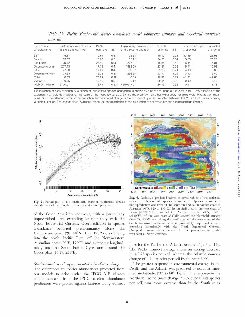
of the South-American continent, with a particularlyimpoverished area extending longitudinally with theNorth Equatorial Current. Overprediction in speciesabundance occurred predominantly along theCalifornian coast (20–408N, 160–1208W), extendinginto the north Pacific Gyre, off the North-easternAustralian coast (208S, 1708E) and extending longitud-inally into the South Pacific Gyre, and around theCocos plate (158N, 2558E).

Species abundance changes associated with climate changeThe differences in species abundances predicted fromour models to arise under the IPCC A1B climatechange scenario from the IPCC baseline abundancepredictions were plotted against latitude along transect

lines for the Pacific and Atlantic oceans (Figs 7 and 8).The Pacific transect average shows an average increasein þ0.75 species per cell, whereas the Atlantic shows achange of þ1.1 species per cell by the year 2199.

The greatest response to environmental change in thePacific and the Atlantic was predicted to occur at inter-mediate latitudes (308 to 608, Fig. 8). The response in theNorthern Pacific (max change �4.5 euphausiid speciesper cell) was more extreme than in the South (max

Table IV: Pacific Euphausiid species abundance model parameter estimates and associated confidenceintervals

Explanatory.variable.name

Explanatory variable valueat the 2.5% quantile

2.5%estimate SE

Explanatory variable valueat the 97.5 % quantile

97.5%estimate SE

Estimate change(nn species)

Estimatedchange %

SST 4.37 5.64 0.31 29.98 19.10 0.52 13.46 29.53Salinity 33.97 15.00 0.51 35.12 24.26 0.64 9.25 20.29Longitude 129.42 23.40 0.90 277.94 16.56 0.62 26.84 215.01Distance to coast 277.43 17.79 0.41 4893.69 22.81 0.68 5.01 10.99SiO3 27.00 17.87 0.47 103.87 22.26 0.71 4.39 9.63Distance to ridge 127.33 18.25 0.57 7286.35 22.17 1.02 3.92 8.60Chl-a 0.03 20.02 0.35 0.49 18.81 0.37 21.21 22.65Vector U 20.25 19.15 0.37 0.17 20.14 0.37 0.99 2.17MLD (May-June) 8770.57 19.61 0.33 5847647.07 20.13 0.39 0.51 1.12

The influence of each explanatory variables on euphausiid species abundance is shown by predictions made at the 2.5% and 97.5% quantiles of theexplanatory variable data values on the scale of the response variable. During the prediction, all other explanatory variables were fixed at their meanvalue. SE is the standard error of the prediction and estimated change is the number of species predicted between the 2.5 and 97.5% explanatoryvariable quantiles. See section titled ‘Statistical modelling’ for description of the calculation of estimated change and percentage change.

Fig. 5. Partial plot of the relationship between euphausiid speciesabundance and the smooth term of sea surface temperature.

Fig. 6. Residuals (predicted minus observed values) of the statisticalmodel prediction of species abundance. Species abundanceunderprediction occurred off the southern and south-eastern coast ofAustralia (408S, 120 to 1508E), the on-shelf area of the west coast ofJapan (408N,1388E), around the Aleutian islands (508N, 1608Eto1408W), off the west coast of Chile around the Humboldt current(5–408S, 808W) and along the shelf area off the west coast of theSouth-American continent, with a particularly impoverished areaextending latitudinally with the North Equatorial Current.Overpredictions were largely restricted to the open ocean, and to thewest coast of North America.


8

at University of S

t Andrew

s on May 3, 2011


ownloaded from


change �1.8 euphausiid species per cell), showing a uni-directional (positive) increase outside the 308 latitudinalband around the equator (308–608). Within this +308latitudinal band, the species abundance showed progress-ive decrease, with the greatest decrease set to occuraround the equator. The greatest change in species percell in the Atlantic was predicted in the northern hemi-sphere (þ3.2 species per cell). Little change was predictedfor the +208 latitudinal band around the equator in theAtlantic. The change in the +108 latitudinal bandaround the equator is expected to resulting in an increas-ing loss in species abundance in the Atlantic, whereas thiszone in the Pacific will see a decrease in species (Fig. 8).The initial (2011–2016) response in the Northern

Atlantic is an oscillating change in species abundance, fol-lowed by a progressive increase in abundance that is stillclimbing by 2199. The South Atlantic will experience amore linear increase in species abundance.

D I S C U S S I O N

Drivers of species abundance

Explanatory variablesThe most important driver of species abundanceincluded in our model was sea surface temperature

Fig. 7. Transect lines (cells in bold) along which potential species abundance changes were investigated in the Pacific and the Atlantic.

Fig. 8. Predicted species abundance difference due to projected environmental change versus latitude in the Pacific and the Atlantic. Speciesabundance is plotted as difference to baseline predictions (2002–2008) along our lines of interest (Fig. 7). Error bars are one standard error fromthe mean. Legend applies to both plots.


9

at University of S

t Andrew

s on May 3, 2011


ownloaded from


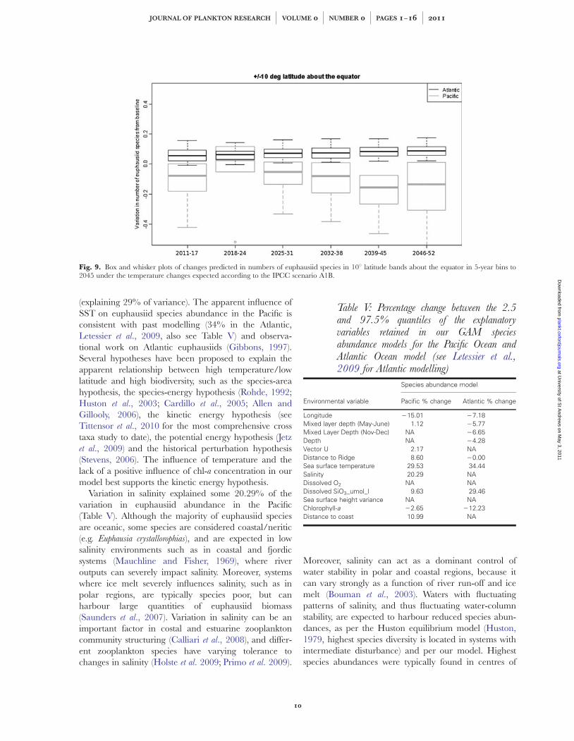
(explaining 29% of variance). The apparent influence ofSST on euphausiid species abundance in the Pacific isconsistent with past modelling (34% in the Atlantic,Letessier et al., 2009, also see Table V) and observa-tional work on Atlantic euphausiids (Gibbons, 1997).Several hypotheses have been proposed to explain theapparent relationship between high temperature/lowlatitude and high biodiversity, such as the species-areahypothesis, the species-energy hypothesis (Rohde, 1992;Huston et al., 2003; Cardillo et al., 2005; Allen andGillooly, 2006), the kinetic energy hypothesis (seeTittensor et al., 2010 for the most comprehensive crosstaxa study to date), the potential energy hypothesis (Jetzet al., 2009) and the historical perturbation hypothesis(Stevens, 2006). The influence of temperature and thelack of a positive influence of chl-a concentration in ourmodel best supports the kinetic energy hypothesis.

Variation in salinity explained some 20.29% of thevariation in euphausiid abundance in the Pacific(Table V). Although the majority of euphausiid speciesare oceanic, some species are considered coastal/neritic(e.g. Euphausia crystallorophias), and are expected in lowsalinity environments such as in coastal and fjordicsystems (Mauchline and Fisher, 1969), where riveroutputs can severely impact salinity. Moreover, systemswhere ice melt severely influences salinity, such as inpolar regions, are typically species poor, but canharbour large quantities of euphausiid biomass(Saunders et al., 2007). Variation in salinity can be animportant factor in costal and estuarine zooplanktoncommunity structuring (Calliari et al., 2008), and differ-ent zooplankton species have varying tolerance tochanges in salinity (Holste et al. 2009; Primo et al. 2009).

Moreover, salinity can act as a dominant control ofwater stability in polar and coastal regions, because itcan vary strongly as a function of river run-off and icemelt (Bouman et al., 2003). Waters with fluctuatingpatterns of salinity, and thus fluctuating water-columnstability, are expected to harbour reduced species abun-dances, as per the Huston equilibrium model (Huston,1979, highest species diversity is located in systems withintermediate disturbance) and per our model. Highestspecies abundances were typically found in centres of

Table V: Percentage change between the 2.5and 97.5% quantiles of the explanatoryvariables retained in our GAM speciesabundance models for the Pacific Ocean andAtlantic Ocean model (see Letessier et al.,2009 for Atlantic modelling)

Environmental variable

Species abundance model

Pacific % change Atlantic % change

Longitude 215.01 27.18Mixed layer depth (May-June) 1.12 25.77Mixed Layer Depth (Nov-Dec) NA 26.65Depth NA 24.28Vector U 2.17 NADistance to Ridge 8.60 20.00Sea surface temperature 29.53 34.44Salinity 20.29 NADissolved O2 NA NADissolved SiO3_umol_l 9.63 29.46Sea surface height variance NA NAChlorophyll-a 22.65 212.23Distance to coast 10.99 NA

Fig. 9. Box and whisker plots of changes predicted in numbers of euphausiid species in 108 latitude bands about the equator in 5-year bins to2045 under the temperature changes expected according to the IPCC scenario A1B.


10

at University of S

t Andrew

s on May 3, 2011


ownloaded from


the subtropical gyres in both hemispheres, where sal-inity is high. Euphausiid species abundance is appar-ently driven higher in stable high salinity waters andlower in unstable polar waters.

The explanatory variable in our model exerting thefifth greatest influence on euphausiid species abundancewas silicate concentration (we discuss the influence ofthe third and fourth driver in context of the basin com-parison, see section ‘Inter-basin comparison’). Althoughthe mechanism behind this relationship is presentlyunclear, it is likely to involve a combination of severalfactors: (i) the silicate concentration control of phyto-plankton growth and diatom growth (Hashioka andYamanaka, 2007); (ii) the increase of zooplankton diver-sity, mediated by non-toxic phytoplankton (Roy, 2008);and (iii) the modification of zooplankton diversity underdifferent regimes of phytoplankton biomass (zooplank-ton diversity is often a unimodal function of phyto-plankton biomass, see Irigoien et al., 2004). Euphausiidgrazing rates are known to vary depending upondiatom species (McClatchie et al., 1991). The sensitivityof euphausiid species abundance to phytoplanktonspecies composition may be mediated throughbottom-up control and tight trophic coupling betweenphytoplankton, primary grazers (such as most copepodspecies, and many euphausiid species, e.g. Thysanoessa

longicaudata, Euphausia superba) and primary/secondaryconsumers (such as some euphausiid species, e.g.Meganyctiphanes norvegica and Nematobrachion boopis,Richardson and Schoeman, 2004). However, ultimatelyour results are at odds with the potential energy hypoth-esis (Jetz et al., 2009), e.g. we do not find a positiverelationship between euphausiid species abundance andprimary production (larger population sizes are sup-ported under greater production regimes, thus sustain-ing niche specialists and reduced extinction rates, seeCurrie et al., 2004). The extent to which silicate concen-tration drives euphausiid species distributions is largelyunknown, and further research to explore these poten-tial bottom-up control pathways is required.

Statistical model residualsThe Pacific model residuals (predicted minus observedvalues) of our species abundance GAM are consistentwith present understanding of oceanographic systems.Zones of underprediction in our Pacific model coincidegeographically with two of Longhurst’s provinces: TheCosta Rican Dome in the North Pacific EquatorialCountercurrent province, and the Tasmanian Sea pro-vince (CRD, PNEC and TASM, respectively, seeLonghurst, 1998). The TASM province is a verydynamic and windy part of the Pacific (Harris et al.,1988; Harris et al., 1991), with primary productivity

patterns typical for provinces at similar latitudes(enhanced spring blooms) and with deep winter-mixedlayer depths. The underprediction by our model herecan be explained, at least partly, by the special geo-graphical and environmental properties of this area.The retroflection of the East Australia Current forms anorthward front across the TASM and Tasman Sea thatseparates bodies of water with very distinct properties;to the north lies the warm Coral Sea and to the southlies the cool Tasman Sea water. It is likely that thisfrontal zone combines species typical of either area,and, in conjunction with enhanced production cascadein the northward flow (Gibbs et al., 1991), causes a loca-lized increase in niche and species abundance whichour model fails to predict.

The PNEC province is defined more on ecologicalgrounds than on oceanographic features (Longhurst,1998) and is, to a large extent, influenced by the pro-ductivity patterns of the Costa Rican dome. This areahas been identified as a hotspot of coastal zooplanktondiversity (Morales-Ramirez, 2008). The isolated natureof the islands of the eastern tropical Pacific has led tothe evolution of many endemic species and the exten-sion of the range of many coastal species (such asEuphausiala melligera), which may explain the underpre-diction of our model (Brinton, 1962).

Underprediction of species abundance in theHumboldt Current may be a consequence of localizedupwelling and associated mixing of different watermasses in this area (Chavez et al., 2003; Ayon et al.,2008). The local fauna is highly adapted to the charac-teristic salinity/high seasonal heterogeneity andenhanced productivity, where endemic zooplanktonspecies proliferate (e.g. Euphausia mucronuta accounts for50% of the mesozooplankton wet weight in winter, andis highly adapted to preying on anchovy eggs, seeKrautz 2003; Antezana, 2010).

Overprediction coincided with the Pacific EquatorialDivergence Province (PEQD, Longhurst, 1998); thedominant characteristic of this biome is the high nitrate,low chlorophyll content of the water. Moreover, this pro-vince has a low productivity regime, typical of highnutrient low carbon biomes. The area has beendescribed as an iron-limited grazer-controlled ecosystem(Price et al., 1994). The overprediction in this provincemay simply be because local production regimes do notsustain high species abundances otherwise typical forsimilar latitudes.

Inter-basin comparisonThe statistical method utilized here is deliberatelysimilar to that employed in our previous study, focussingon drivers of variability in Atlantic euphausiid


11

at University of S

t Andrew

s on May 3, 2011


ownloaded from


abundance and diversity (Letessier et al., 2009). Theenvironmental and biological data considered in bothwere retrieved from the same online and publishedsources. Overall, the directions of the responses to theimportant variables (sea surface temperature, longitude,silicate concentration) were similar in the Pacific andthe Atlantic (Table V).

In both ocean models, we observed an eastwardsdecrease in species abundance (longitude was respon-sible for 15 and 7% species abundance reduction in thePacific and Atlantic, respectively). On the eastern sideof the two oceans, the major currents transport coolwater toward the tropics, meaning that the warm tropi-cal seas will span a broad latitudinal range in the westbut not in the east (Fig. 3), and communities will betypical of higher latitudes in the east. The observed pat-terns are probably a function of the predominance ofupwelling on the east coast of the Atlantic and thePacific (Brown et al., 1989).

A total of 81 euphausiid species had ranges withinour Pacific survey grid, a greater number than in theAtlantic (54 species). Moreover, our Pacific modellinghas revealed several variables to be significant here thatwere not significant in the Atlantic study (e.g. Currentvector U, Distance to coast, Distance to ridge; Table V).The Pacific Ocean is, by some estimates, close to abillion years old (The Open University, 1998) and is, assuch, much older than the Atlantic (150 million years).The last common ancestor of the Euphausiidea lived�130 mya and most modern genera were presentbefore 23 mya (Jarman, 2001). Since then, the Pacifichas undergone relatively few geological changes com-pared to the Atlantic. Furthermore, the Atlantic hasbecome separated from the Indopacific, a source ofradiative diversity (in the late Miocene, some 7 myaago). That and the large area of the Pacific (32% of thesurface of the Earth) have been proposed as the expla-nation for the greater overall abundance of marinespecies observed in the Pacific Ocean (Briggs, 1999;Williams, 2007) and, in this case, the increased modelcomplexity compared to the Atlantic. The large size ofthe Pacific makes the distribution of its fauna susceptibleto a greater scope of external factors and environmentalvariables.

The Atlantic study was largely restricted to the mid-ocean, as our sampling grid specifically omitted conti-nental shelves and marginal sectors and was constructedwith the specific objective of enabling testing of hypoth-eses to do with the influences of bathymetric features(such as ridges and fracture zones) on additional diver-sity and abundance. This might explain the influence ofproximity to coast in the Pacific: according to ourmodel, proximity to land serves to reduce the number

of species. The comparison between oceans will not becompletely bias-free because of the different grids usedin each. However, the two oceans have fundamentallydifferent characteristics in terms of basin dimension,and any completely uniform grid will hold someinherent bias. The number of cells covering shelf sectorsin the Pacific (average seabed depth shallower than500 m, n ¼ 11) only amounted to some 0.4% of thetotal grid, and had they not been included our con-clusions would probably not have changed. The differ-ences we expose here between the Atlantic andthe Pacific (Table V) are at odds with of the results ofTittensor et al. (2010) who suggest, following analysis ofa global data set of diversity, that variability in oceanbasin (i.e. Pacific, Atlantic, Indian) is not a significantvariable in global diversity.

Species abundance changes with temperature riseOur data show that the species abundance of euphau-siids in the Pacific is influenced less by SST variability(some �5% difference in between the quantiles) than inthe Atlantic (Table V). Moreover, the higher abundanceof Pacific euphausiid species (81 from our data set)means that every degree change in SST will increasethe euphausiid species abundance per cell by 0.52, asopposed to 0.70 in the Atlantic (assuming linear changebetween the quantiles). All else remaining equal, ourmodel predicts that the distributions of Pacific euphau-siid species abundance will be more resistant to climatechange than the Atlantic.

The functions of marine and terrestrial biologicalprocesses are predicted to change as a consequence ofpresent and future anthropogenic climate change.However, whereas environmental changes might bequantifiable, the biological responses are harder topredict and usually involve considerable speculation (seeBrierley and Kingsford, 2009, and Walther, 2010 for areview of potential marine and terrestrial changes,respectively). Our model is no exception. We haveextrapolated assuming a consistent response to tempera-ture, and by holding all other variables equal.

Both oceans will on average see an increase inspecies abundance per cell. Although the greatestincrease in species abundance is predicted to take placein the Pacific (maximum increase þ4.5 species in thePacific versus þ3 species per cell in the Atlantic), thePacific will, on average, experience less change than inthe Atlantic (þ0.75 species per cell versus þ1.1) by theyear 2199, thus confirming our earlier predictionsregarding the difference in sensitivity between the twobasins (see first paragraph this section). Moreover, ourmodel predictions suggest that the species abundance inthe +208 latitude band around the equator will


12

at University of S

t Andrew

s on May 3, 2011


ownloaded from


experience little changes in the Atlantic, whereas thePacific will see a decrease. Our results suggest that thepresent broad patterns apparent in species abundance(low in high latitudes, high in intermediate latitudes andintermediate in the tropics) will become less pro-nounced in a warming ocean; eventually species abun-dance will be enhanced within intermediate-to-highlatitudes (308N to 608N and 308S to 608S) and dimin-ished in the tropics (208N to 208S). The predictedchange of species abundance (less marked in thetropics, more pronounced at intermediate to high lati-tudes) is consistent with changes already observed to beoccurring in terrestrial systems in Europe and America(Rosenzweig et al., 2008); however, recent evidencepoints to increased vulnerability in tropical ectotherms(Dilling and Alldredge, 2000). The changes we predictat intermediate latitudes (308 to 608) are consistent withalready-observed changes in zooplankton assemblagesin the North Atlantic (i.e. communities shifting north,see Beaugrand et al., 2002; Beaugrand and Ibanez,2004; Richardson and Schoeman, 2004). This studyprovides some evidence that shifts in species abun-dances may not be restricted to the North Atlantic zoo-plankton community but rather are symptomatic ofresponses to climate change at the same latitudes in theAtlantic and the Pacific.

We opted to consider variability models for themoderate A1B scenario from the IntergovernmentalPanel on Climate Change (IPCC), which providesenvironmental variable predictions under assumptionsregarding anthropogenic impact on climate deemed tobe ‘intermediate’ (O’Neill and Oppenheimer, 2002).However, annual CO2 emission increases (.2 parts permillions, Goodwin and Lenton, 2009) are surpassingthe worst-case scenario of the IPCC (scenario A2IPCC, 2007b), and it is likely that our choice is conser-vative. Changes in euphausiid communities, as withother ecosystems changes (Jackson 2008), may be morepronounced than expected.

CO N C LU S I O N

Our Pacific species abundance model confirms theimportance of sea surface temperature as a speciesabundance driver, but also elucidates other less familiarpredictors. Our model is informative in that it bringstogether a large body of information without makingany assumptions regarding relationships betweenspecies abundance and environmental variables. Ourstudy does not integrate other effects, such as overfish-ing, pollution and the migration/transportation ofspecies between oceans (Reid et al., 2007; Greene et al.,

2008). We have shown that there are substantialresiduals in the species abundance/temperature modelin some locations, and that lesser known drivers such assilicate concentration, salinity and longitude are also sig-nificant predictors of euphausiid species abundance inthe Atlantic and Pacific. Our model framework is rel-evant for future climate changes; thus we have success-fully demonstrated latitudinal heterogeneity to climatechange in species abundance predictions, and describeddifferent potential responses to climate change in eachbasin. From a conservation perspective, simplifying to aspecies abundance/temperature relationship (Tittensoret al., 2010) is potentially dangerous since it may divertattention from other ocean characteristics, such as nutri-ent concentration, that play critical roles in ecosystemfunction.

S U P P L E M E N TA RY DATA

Supplementary data can be found online at http://plankt.oxfordjournals.org.

AC K N OW L E D G E M E N T S

We thank Dr Thomas Sturgeon for help and advicewith the handling of binary data. We thankMr A. Cousin and Mr A. Bishop for help during theconstruction of the grid, and Clint Blight for help andsupport with Geographical Information System soft-ware. The images and data used in this study wereacquired using the GES-DISC Interactive OnlineVisualization ANdaNalysis Infrastructure (Giovanni) aspart of the NASA’s Goddard Earth Sciences (GES)Data and Information Services Center (DISC).

F U N D I N G

We thank the United Kingdom Natural EnvironmentResearch Council (NERC, grant number: NE/C513018/1) and the School of Biology at theUniversity of St Andrews for funding.

R E F E R E N C E S

Akaike, H. (1973) Information Theory and an extension of themaximum likelihood. In Petrov, B. N. and Cs’aki, F. (eds) Proceedings

of the 2nd International Symposium on Information Theory. Budapest:Academiai Kiado, pp. 267–281.


13

at University of S

t Andrew

s on May 3, 2011


ownloaded from

http://plankt.oxfordjournals.org/cgi/content/full/fbr033/DC1




Allen, A. P. and Gillooly, J. (2006) Assessing latitudinal gradients inspeciation rates and biodiversity at the global scale. Ecol. Lett., 9,947–954.

Antezana, T. (2010) Euphausia mucronata: a keystone herbivore and preyof the Humboldt Current System. Deep Sea Res. II Top. Stud.

Oceanogr., 57, 652–662.

Ayon, P., Criales-Hernandez, M. I., Schwamborn, R. et al. (2008)Zooplankton research off Peru: a review. Prog. Oceanogr., 79,238–255.

Barkley, R. A. (1968) Oceanographic Atlas of the Pacific Ocean. University ofHawaii Press, Honolulu.

Beaugrand, G. and Ibanez, F. (2004) Monitoring marine planktonecosystems. II: long-term changes in North Sea calanoid copepodsin relation to hydro-climatic variability. Mar. Ecol. Prog. Ser., 284,35–47.

Beaugrand, G., Reid, P. C., Ibanez, F. et al. (2002) Reorganization ofNorth Atlantic marine copepod biodiversity and climate. Science,296, 1692–1694.

Bonjean, F. and Lagerhoed, G. S. (2002) Diagnostic model and analy-sis of the surface currents in the Tropical Pacific Ocean. J. Phys.

Oceanogr., 32, 2930–2954.

Bouman, H., Platt, T., Sathyendranath, S. et al. (2003) Temperature asindicator of optical properties and community structure of marinephytoplankton: implications for remote sensing. Mar. Ecol. Prog. Ser.,258, 19–30.

Brierley, A. S. and Cox, M. J. (2010) Shapes of krill swarms and fishschools emerge as aggregation members avoid predators and accessoxygen. Curr. Biol., 20, 1758–1762.

Brierley, A. S. and Kingsford, M. J. (2009) Impacts of climatechange on marine organisms and ecosystems. Curr. Biol., 19,R602–R614.

Briggs, J. C. (1999) Coincident biogeographic patterns: Indo-WestPacific Ocean. Evolution, 53, 326–335.

Brinton, E. (1962) The distribution of Pacific euphausiids. Bull. Scripps

Inst. Oceanogr., 8, 21–270.

Brinton, E., Ohman, M. D., Townsend, A.W. et al. (2000) Euphausiidsof the World Ocean World Biodiversity Database CD-ROM Series.Springer UNESCO.

Brown, E., Colling, A., Park, D. et al. (1989) Ocean Circulation. TheOpen University, Boston.

Burnham, K. P. and Anderson, D. R. (2002) Model Selection and

Multimodel Inference. Springer, New York.

Calliari, D., Borg, M. C., Thor, P. et al. (2008) Instantaneous salinityreductions affect the survival and feeding rates of the co-occurringcopepods Acartia tonsa Dana and A. clausi Giesbrecht differently.J. Exp. Mar. Biol. Ecol., 362, 18–25.

Cardillo, M., Orme, C. D. and Owens, I. P. (2005) Testing for latitudi-nal bias in diversification rates: an example using New World birds.Ecology, 86, 2278–2287.

Chavez, F. P., Ryan, J., Lluch-Cota, S. E. et al. (2003) From anchoviesto sardines and back: multidecadal change in the Pacific Ocean.Science, 299, 217–221.

Chelton, B. D., deSzoeke, R. A. and Schlax, M. G. (2008) Global Atlas

of First-Baroclinic Rossby Radius of Deformation and Gravity-Wave Phase

Speed. Oregon State University.

Chiles, J. and Delpiner, P. (1999) Geostatistics: Modeling SpatialUncertainty. John Wiley and Sons, New York.

Clarke, A. J. and Dottori, M. (2008) Planetary wave propagation offCalifornia and its effect on zooplankton. J. Phys. Oceanogr., 38,702–714.

Clarke, A. and Gaston, K. J. (2006) Climate, energy and diversity.Proc. R Soc. Biol. Sci., 273, 2257–2266.

Clarke, A. and Tyler, P. A. (2008) Adult antarctic krill feeding atabyssal depths. Curr. Biol., 18, 282–285.

Cressie, N. (1991) Statistics for Spatial Data. John Wiley & Sons,New York.

Currie, D. J., Mittelbach, G. and Cornell, H. (2004) Predictions andtests of climate-based hypotheses of broad-scale variation in taxo-nomic richness. Ecol. Lett., 7, 1121–1134.

Development Team C. (2007) R: A Language and Environment for Statistical

Computing. R Foundation for Statistical Computing, Vienna.

Dilling, L. and Alldredge, A. (2000) Fragmentation of marine snow byswimming macrozooplankton: a new process impacting carboncycling in the sea. Deep Sea Res. I Oceanogr. Res. Pap., 47, 1227–1245.

Ducet, N., Le Traon, P. Y. and Reverdin, G. (2000) Global high-resolution mapping of ocean circulation from TOPEX/Poseidonand ERS-1 and-2. J. Geophys. Res. Oceans, 105, 19477–19499.

Fuhrman, J. A., Steele, J. A., Hewson, I. et al. (2008) A latitudinaldiversity gradient in planktonic marine bacteria. Proc. Natl. Acad. Sci.

USA, 105, 7774–7778.

Gibbons, M. J. (1997) Pelagic biogeography of the South AtlanticOcean. Mar. Biol., 129, 757–768.

Gibbs, C. F., Arnott, G. H., Longmore, A. R. et al. (1991) Nutrientand plankton distribution near a shelf break front in the region ofthe bass strait cascade. Aust. J. Mar. Freshwater Res., 42, 201–217.

Goodwin, P. and Lenton, T. M. (2009) Quantifying the feedbackbetween ocean heating and CO2 solubility as an equivalent carbonemission. Geophys. Res. Lett., 36, 5.

Greene, C. H., Pershing, A. J., Cronin, T. M. et al. (2008) Arcticclimate change and its impacts on the ecology of the NorthAtlantic. Ecology, 89, S24–S38.

Harris, G. P., Davies, P., Nunez, M. et al. (1988) Interannual variabilityin climate and fisheries in Tasmania. Nature, 333, 754–757.

Harris, G. P., Griffiths, F. B., Clementson, L. A. et al. (1991) Seasonaland interannual variability in physical processes, nutrient cyclingand the structure of the food-chain in Tasmanian shelf waters.J. Plankton Res., 13, S109–S131.

Hashioka, T. and Yamanaka, Y. (2007) Seasonal and regionalvariations of phytoplankton groups by top-down and bottom-upcontrols obtained by a 3D ecosystem model. Ecol. Model., 202,68–80.

Holste, L., John, M. A. and Peck, M. A. (2009) The effects of temp-erature and salinity on reproductive success of Temora longicornis inthe Baltic Sea: a copepod coping with a tough situation. Mar. Biol.,156, 527–540.

Hox, J. J. (2002) Some important methodological and statistical issues.In: Multilevel Analysis: Techniques and Applications Illustrate. Routledge.

Huntley, M. E. and Niiler, P. P. (1995) Physical control of populationdynamics in the Southern Ocean. ICES J. Mar. Sci., 52(3–4),457–468.

Huston, M. A. (1979) A general hypothesis of species diversity. Am.

Nat., 113, 81–101.

Huston, M. A., Brown, J. H., Allen, A. P. et al. (2003) Heat and biodi-versity. Science, 299, 512.


14

at University of S

t Andrew

s on May 3, 2011


ownloaded from


IPCC (2007a) Climate change: the physical science basis. In Solomon,S., Qin, D., Manning, M., Chen, Z., Marquis, M., Averyt, K. B.,Tignor, M., Miller, H. L. (eds), Contribution of Working Group I tothe Fourth Assessment Report of the Intergovernmental Panel onClimate Change. Cambridge University Press, Cambridge.

IPCC (2007b) Background and overview. In Nakicenovic, N., Swart,R. (eds), Special Reports on Emission Scenarios. Cambridge UniversityPress, Cambridge.

Irigoien, X., Huisman, J. and Harris, R. P. (2004) Global biodiversitypatterns of marine phytoplankton and zooplankton. Nature, 429,863–867.

Jackson, J.B.C. (2008) Ecological extinction and evolution in the bravenew ocean. Proc. Natl. Acad. Sci. USA, 105, 11458–11465.

Jarman, S. N. (2001) The evolutionary history of krill inferred fromnuclear large subunit rDNA sequence analysis. Biol. J. Linnean Soc.,1, 199–212.

Jetz, W., Kreft, H., Ceballos, G. et al. (2009) Global associationsbetween terrestrial producer and vertebrate consumer diversity. Proc.

R. Soc. Biol. Sci. Ser., B276, 269–278.

Kara, A. B., Rochford, P. A. and Hurlburt, H. E. (2002) NavalResearch Laboratory Mixed Layer Depth (NMLD) Climatologies.Washington DC. NRL Report 22.

Kim, H. S. (2010) Population dynamics of the euphausiids Euphausia

pacifica and Thysanoessa inspinata in the Oyashio region during the2007 spring phytoplankton bloom. Deep-Sea Research Part II - Topical

Studies in Oceanography, 57, 1727–1732.

Krautz, M. (2003) Detection of anchoveta (Engraulis ringens Jenyns1842) eggs in euphausiid diets using immunoassays (ELISA). J. Exp.

Mar. Biol. Ecol., 294, 27–39.

Letessier, T. B., Cox, M. J. and Brierley, A. S. (2009) Drivers ofeuphausiid species abundance and numerical abundance in theAtlantic Ocean. Mar. Biol., 156, 2539–2553.

Lindley, J. A. (1977) Continuous plankton records: the distribution ofthe Euphausiacea (Crustacea: Malacostraca) in the north Atlanticand the North Sea, 1966–1967. J. Biogeogr., 4, 121–133.

Longhurst, A. (1998) Ecological Geography of the Sea. Academic Press, SanDiego.

Mauchline, J. and Fisher, L. R. (1969) The biology of euphausiids.Adv. Mar. Biol., 7, 1–454.

McClatchie, S., Jaquiery, P., Kawachi, R. et al. (1991) Grazing rates ofNyctiphanes australis (Euphausiacea) in the laboratory and OtagoHarbour, New Zealand, measured using three independentmethods. Cont. Shelf Res., 11, 1–22.

Morales-Ramirez, A. (2008) Qualitative characterization of the zoo-plankton of the Cocos Island Marine Conservation Area (Area deConservacion Marina Isla del Coco, ACMIC), Pacific Ocean ofCosta Rica. Rev. Biol. Trop., 56, 159–169.

Murase, H., Nagashima, H., Yonezaki, S. et al. (2009) Application of ageneralized additive model (GAM) to reveal relationships betweenenvironmental factors and distributions of pelagic fish and krill: acase study in Sendai Bay, Japan. ICES J. Mar. Sci., 6, 1417–1424.

O’Neill, B. C. and Oppenheimer, M. (2002) Climate change—danger-ous climate impacts and the Kyoto protocol. Science, 296, 1971–1972.

Osborne, J. and Flinchem, E. P. (1994) Ocean Atlas. Java Ocean Atlas.

Pinheiro, J. C. and Bates, D. M. (2000) Mixed-Effects Models in S and

S-PLUS. Springer.

Piontkovski, S. A., Williams, R., Peterson, W. et al. (1995) Relationshipbetween oceanic mesozooplankton and energy of eddy fields. Mar.

Ecol. Prog. Ser., 128, 35–41.

Pitcher, T. J. (2008) The sea ahead: challenges to marine biology fromseafood sustainability. Hydrobiologia, 606, 161–185.

Potts, J. M. and Elith, J. (2006) Comparing species abundance models.Ecol. Model., 199, 153–163.

Price, N. M., Ahner, B. A. and Morel, F. M. (1994) The equatorialPacific Ocean: grazer-controlled phytoplankton populations in aniron-limited ecosystem. Limnol. Oceanogr., 39, 520–534.

Primo, A. L., Azeiteiro, U. M., Marques, S. C. et al. (2009) Changesin zooplankton diversity and distribution pattern under varying pre-cipitation regimes in a southern temperate estuary. Estuarine Coastal

Shelf Sci., 82, 341–347.

R Development Core Team (2007) R: a language and environmentfor statistical computing, reference index version 2.5.1. R Foundationfor Statistical Computing, Vienna. ISBN 3-900051- 07-0,http://www.R-project.org.

Reid, P. C., Johns, D. G., Edwards, M. et al. (2007) A biological conse-quence of reducing Arctic ice cover: arrival of the Pacific diatomNeodenticula seminae in the North Atlantic for the first time in 800000 years. Global Change Biol., 13, 1910–1921.

Richardson, A. J. and Schoeman, D. S. (2004) Climate impact onplankton ecosystems in the Northeast Atlantic. Science, 305,1609–1612.

Rohde, K. (1992) Latitudinal gradients in species diversity: the searchfor the primary cause. Oikos, 65, 514–527.

Rosenzweig, C., Karoly, D., Vicarelli, M. et al. (2008) Attributing phys-ical and biological impacts to anthropogenic climate change. Nature,453, 353–357.

Roy, S. (2008) Spatial interaction among nontoxic phytoplankton,toxic phytoplankton, and zooplankton: emergence in space andtime. J. Biol. Phys., 34, 459–474.

Rutherford, S., D’Hondt, S. and Prell, W. (1999) Environmental con-trols on the geographic distribution of zooplankton diversity. Nature,400, 749–753.

Saunders, R. A., Ingvarsdottir, A. and Rasmussen, J. (2007) Regionalvariation in distribution pattern, population structure andgrowth rates of Meganyctiphanes norvegica and Thysanoessa

longicaudata in the Irminger Sea, North Atlantic. Prog. Oceanogr., 72,313–342.

Schnack-Schiel, S. B. and Isla, E. (2005) The role of zooplankton inthe pelagic-benthic coupling of the Southern Ocean. Sci. Mar., 69,39–55.

Stevens, R. D. (2006) Historical processes enhance patterns of diversityalong latitudinal gradients. Proc. R. Soc. Biol. Sci., 273, 2283–2289.

Tarling, G. A. and Johnson, M. L. (2006) Satiation gives krill thatsinking feeling. Curr. Biol., 16, R83–R84.

The Open University. (1998) The Ocean Basins: Their structure and evol-

ution. Walton Hall.

Tittensor, D. P., Mora, C., Jetz, W. et al. (2010) Global patterns andpredictors of marine biodiversity across taxa. Nature, 466,1098–1101.

Trathan, P. N., Priddle, J., Watkins, J. L. et al. (1993) Spatial variabilityof Antarctic krill in relation to mesoscale hydrography. Mar. Ecol.

Prog. Ser., 98, 61–71.


15

at University of S

t Andrew

s on May 3, 2011


ownloaded from

http://www.R-project.org

http://www.R-project.org


Verity, P. G., Smetacek, V. and Smayda, T. J. (2002) Status, trends andthe future of the marine pelagic ecosystem. Environ. Conserv., 29,207–237.

Walther, G. (2010) Community and ecosystem responses to recentclimate change. Phil. Trans. R Soc. London. Ser. B Biol. Sci., 365,2019–2024.

Williams, S. T. (2007) Origins and diversification of Indo-WestPacific marine fauna: evolutionary history and biogeography ofturban shells (Gastropoda, Turbinidae). Biol. J. Linn Soc., 92,573–592.

Wood, S. (2006) Generalized Additive Models: An Introduction with R.Chapman & Hall/CRC, London.


16

at University of S

t Andrew

s on May 3, 2011


ownloaded from


Drivers of variability in Euphausiid species abundance throughout

Documents

Transcript of Drivers of variability in Euphausiid species abundance throughout