Nova Southeastern University Nova Southeastern University

NSUWorks NSUWorks

HCNSO Student Theses and Dissertations HCNSO Student Work

4-29-2020

A Temporal Analysis of the Euphausiid Assemblage in the Gulf of A Temporal Analysis of the Euphausiid Assemblage in the Gulf of

Mexico after the Deepwater Horizon Oil Spill, with Notes on Mexico after the Deepwater Horizon Oil Spill, with Notes on

Seasonal Reproduction Seasonal Reproduction

Nathan A. La Spina Nova Southeastern University

Follow this and additional works at: https://nsuworks.nova.edu/occ_stuetd

Part of the Marine Biology Commons, and the Oceanography and Atmospheric Sciences and

Meteorology Commons

Share Feedback About This Item

NSUWorks Citation NSUWorks Citation Nathan A. La Spina. 2020. A Temporal Analysis of the Euphausiid Assemblage in the Gulf of Mexico after the Deepwater Horizon Oil Spill, with Notes on Seasonal Reproduction. Master's thesis. Nova Southeastern University. Retrieved from NSUWorks, . (531) https://nsuworks.nova.edu/occ_stuetd/531.

This Thesis is brought to you by the HCNSO Student Work at NSUWorks. It has been accepted for inclusion in HCNSO Student Theses and Dissertations by an authorized administrator of NSUWorks. For more information, please contact nsuworks@nova.edu.

Thesis of Nathan A. La Spina

Submitted in Partial Fulfillment of the Requirements for the Degree of

Master of Science M.S. Marine Biology

Nova Southeastern University Halmos College of Natural Sciences and Oceanography

April 2020

Approved: Thesis Committee

Major Professor: Dr. Tamara Frank

Committee Member: Dr. Tracey T. Sutton

Committee Member: Dr. Christopher Blanar

Committee Member: Dr. Bernhard Riegl

This thesis is available at NSUWorks: https://nsuworks.nova.edu/occ_stuetd/531

1

Nova Southeastern University

Halmos College of Natural Sciences

And Oceanography

A Temporal Analysis of the Euphausiid Assemblage in the Gulf of Mexico after the Deepwater

Horizon Oil Spill, with Notes on Seasonal Reproduction

By Nathan Andrew LaSpina

Submitted to the Faculty of

Nova Southeastern University

Halmos College of Natural Sciences and Oceanography

in partial fulfillment of the requirements for

the degree of Master of Science with a specialty in:

Marine Biology

Nova Southeastern University

Date: 05/27/2020

2

Table of contents

Acknowledgments 3

List of Tables 4

List of Figures 5

Abstract 6

Introduction 7

Materials and Methods 9

Statistical Analysis 11

Results 13

Seasonal effects on the assemblage abundance, biomass, and reproduction 13

Temporal effects on the assemblage abundance, biomass, and mean total length 16

Discussion 22

Seasonal variability and reproduction 22

Temporal changes in the assemblage 23

Conclusions 26

Appendices 32

3

Acknowledgments

Funding for this thesis came from the National Oceanographic and Atmospheric Administration,

the Gulf of Mexico Research Initiative, and Nova Southeastern University. I would like to thank

each organization for providing the resources which allowed me to complete this work.

I thank my major advisor, Dr. Tamara Frank, for her unwavering support which enabled me to

further develop my writing and critical thinking skills. I am extremely grateful for her guidance,

generosity, and patience. To my committee members, Dr. Tracey Sutton, Dr. Bernhard Riegl and

Dr. Christopher Blanar, I thank you for providing your expertise and helping me tackle the

questions I had along the way. I would also like to especially thank Dr. Rosanna Milligan for

guiding me through the rough seas that are the fields of statistics and computer coding. Thank

you, Dr. Milligan, for your patience and personalized tutelage. In addition, I would like to thank

April Cook for assisting me with sorting through the data and getting everything ready for my

analysis. To my lab mates, both past and present, I thank you all for the help you have given me

and the great times we had. Finally, I thank my wife, my son, and my parents, without whom I

would not have completed such an undertaking. They are my foundation and the voices in my

heart that told me to never quit.

4

List of Tables

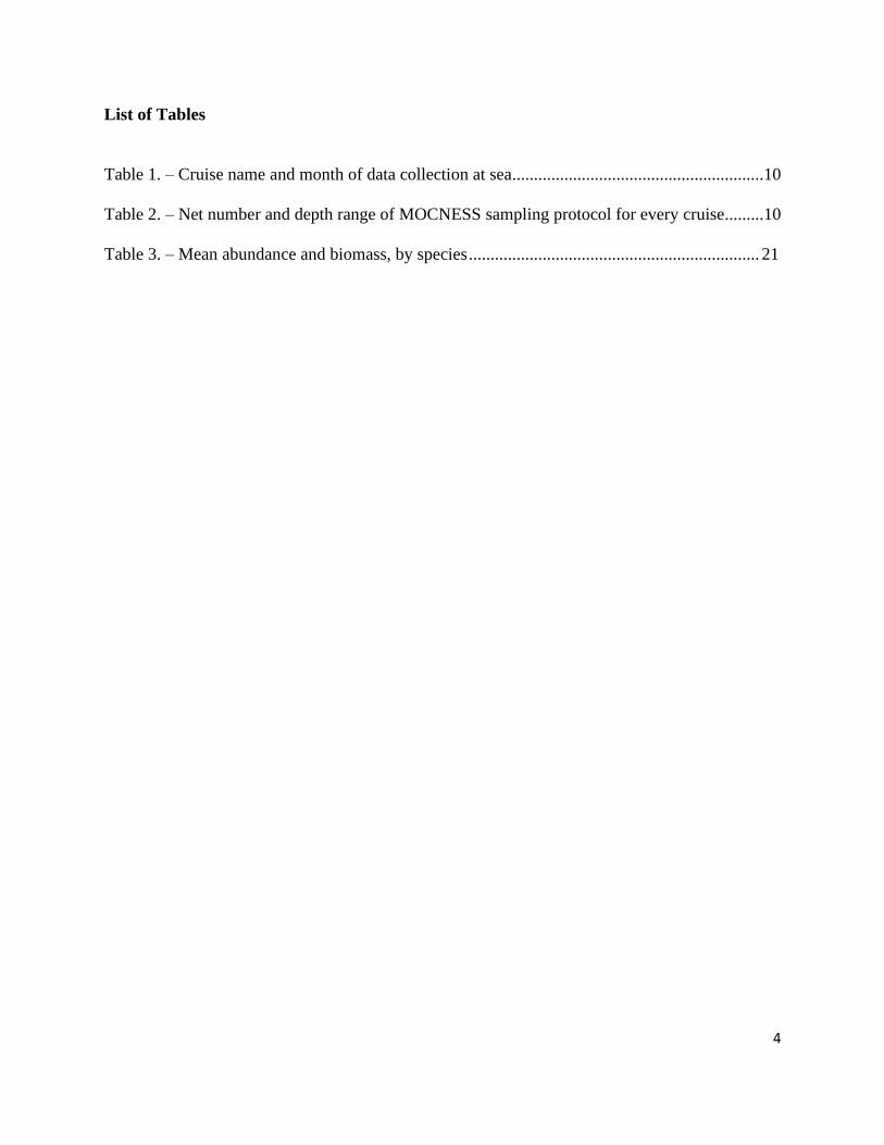
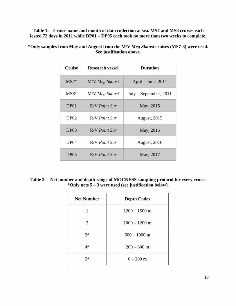
Table 1. – Cruise name and month of data collection at sea..........................................................10

Table 2. – Net number and depth range of MOCNESS sampling protocol for every cruise.........10

Table 3. – Mean abundance and biomass, by species ................................................................... 21

5

List of Figures

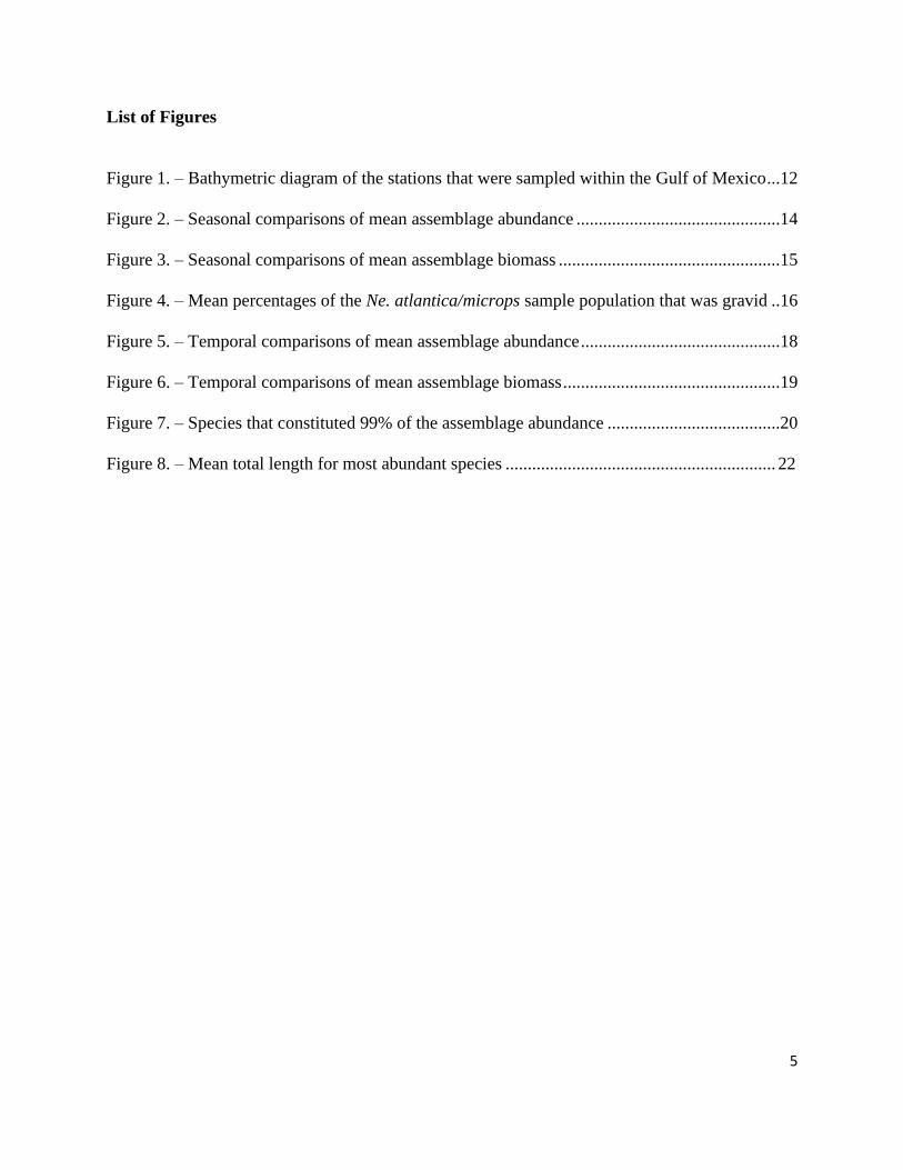
Figure 1. – Bathymetric diagram of the stations that were sampled within the Gulf of Mexico ...12

Figure 2. – Seasonal comparisons of mean assemblage abundance ..............................................14

Figure 3. – Seasonal comparisons of mean assemblage biomass ..................................................15

Figure 4. – Mean percentages of the Ne. atlantica/microps sample population that was gravid ..16

Figure 5. – Temporal comparisons of mean assemblage abundance .............................................18

Figure 6. – Temporal comparisons of mean assemblage biomass .................................................19

Figure 7. – Species that constituted 99% of the assemblage abundance .......................................20

Figure 8. – Mean total length for most abundant species ............................................................. 22

6

Abstract

A Temporal Analysis of the Euphausiid Assemblage in the Gulf of Mexico after the Deepwater

Horizon Oil Spill, with Notes on Seasonal Reproduction

This thesis presents the results of the first multi-year study on the euphausiid assemblage in the

vicinity of the Deepwater Horizon oil spill (DWHOS), covering depths down to 1000 m. There

are no data on the euphausiid assemblage from this region prior to the oil spill; therefore, the data

in this study were analyzed with respect to year (samples collected in 2011 vs. those collected

between 2015 – 2016), and season (May vs. August) to determine if any trends were present.

These results presented here show a statistically significant decrease in both abundance and

biomass between 2011 and 2015 – 2016, indicating that the assemblage has been declining since

2011, along with a continued decline from May 2016 to May 2017. Seasonal effects were also

present, as abundance and biomass were statistically higher in May than in August in both 2011

and 2016. In addition, the percentage of gravid females of the grouped species, Nematoscelis

atlantica/microps, was also higher in May for both years, but only statistically significant in

2016. This seasonal variability may possibly be linked to food availability as a result of seasonal

phytoplankton blooms. The information presented here will act as a reference point for future

studies in the Gulf of Mexico (GOM), to aid in understanding how the euphausiid assemblage

responds to anthropogenic events.

Key words: Euphausiidae, Pelagic Crustaceans, Seasonality, Deepwater Horizon Oil Spill.

7

Introduction

Euphausiids constitute about 40% of the biomass within the world’s oceans and are

important to the diets of many higher trophic level consumers (Simard et al. 1986; Pillar and

Stuart 1988; Kinsey and Hopkins 1994; Dalpadado and Skjoldal 1996; Nicol and Endo 1997;

Castellanos and Morales 2009; Kaplan et al. 2013). A number of whale species, including blue

(Balaenoptera musculus), minke (Balaenoptera acutorostrata), fin (Balaenoptera physalus),

humpback (Megaptera novaeangliae), Bryde's (Balaenoptera brydei), and sei whales

(Balaenoptera borealis) all rely on euphausiids to sustain themselves (Strickland et al. 1970;

Schoenherr 1991). Many other animals such as fishes (Robinson 2000; Jayalakshmi et al. 2011),

seabirds (Deagle et al. 2007), seals (Bradshaw et al. 2003), squid (Cargnelli et al. 1999), and

humans harvest euphausiids as a source of food as well (Nicol and Endo 1999). Because

euphausiids are so widely distributed and play such a vital role in many regional food webs, a

reduction in their numbers could be detrimental to many higher trophic level species.

Of the 86 documented species of euphausiids, 34 can be found in the GOM (Castellanos

and Morales 2009; Felder and Camp 2009). Euphausiids are classified as either zooplankton or

micronekton, depending on their size and current life history phase. Larval phase individuals,

which are in the zooplankton phase of their life, are typically less than five mm in length, while

mature adults of many species are considered micronekton (Brinton 1962; Brinton et al. 1999).

Euphausiids typically live about two to three years in the wild; however, laboratory results

suggest that some species of euphausiids that live near Antarctica, such as Euphausia superba,

can live for 11 years (Einarsson 1945; Mackintosh 1972; Ikeda 1985).

There have been previous studies on the euphausiid assemblage in the GOM, but none

that reach the geographical or temporal range of the work presented in this thesis. Gasca et al.

(2001) completed work on the spatial distribution of these animals within the photic zone, at

depths of only 0 – 200 m, in the southern part of the Gulf, while Kinsey and Hopkins (1994)

collected data on the diet of euphausiids, from the surface waters down to 1000 m, during the

summer months of 1975 – 1977, at one location in the northeastern Gulf that they referred to as

Standard Station (Kinsey and Hopkins 1994; Gasca et al. 2001). In 2016, Fine and Frank

described the euphausiid assemblage in the northern GOM following the DWHOS, but this study

was limited to data collected from April – June of 2011 (Fine 2016; Frank et al. 2020). One of

their primary finding was that euphausiid abundance and biomass were significantly higher at

8

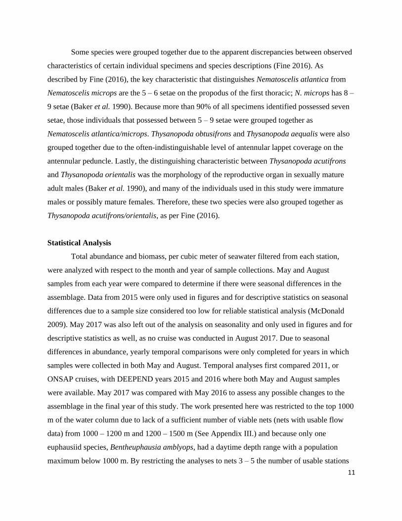
slope stations, stations on the landward size of the 1000 m isobath, than offshore stations,

stations on the ocean side of the 1000 m isobath, (Figure 1). For this reason, only samples

associated with offshore sites were used in the study presented in this thesis.

The location of this study is of particular interest because it is the site of the 2010

Deepwater Horizon oil spill (DWHOS). The DWHOS is the largest aquatic oil spill in U.S.

history, releasing nearly five million barrels of Louisiana Sweet Crude oil from a leak that

occurred at 1500 m depth (Abbriano et al. 2011; McNutt et al. 2012). The effects of the oil spill

on deep-sea crustaceans remain difficult to determine because no baseline data are available for

this region prior to the oil spill (Fine 2016; Burdett et al. 2017; Nichols 2018). However, the

abundance of four fish taxa larvae declined in 2010 compared to the three years before the oil

spill, which may have resulted from a detrimental effect of oil and dispersants, although natural

inter-annual variability cannot be discounted as the basis of the decline (Rooker et al. 2013).

Another study examined near-slope mesozooplankton communities, for which pre-spill baseline

data were available, and hypothesized that it was highly plausible that the DWHOS was the

reason for the initial decline in zooplankton densities, which included euphausiid protozoea

(Carassou et al. 2014). However, Carassou et al. (2014) only examined zooplankton within the

top 200 m of near-slope waters off the coast of Louisiana. Regardless of the cause, increased

mortality amongst euphausiids may be detrimental to the stability of the local marine ecosystem.

The modelling study of Kaplan et al. (2013) showed that when euphausiids along the California

coast are harvested to 40% of unfished levels, the result would be a reduction in abundance of

more than 20% for nearly one-third of all other groups within their food web. The major goal of

this thesis was to determine whether there was a temporal change in the assemblage in the

vicinity of the DWHOS, incorporating data from samples collected from offshore stations, in

both May and August of 2011, 2015, 2016, as well as May 2017, from 1000 m to the surface,

with consideration given to seasonal variations that may skew the results.

9

Materials and Methods

Euphausiids were analyzed from samples collected on two cruises onboard the M/V Meg

Skansi (as part of the ONSAP studies) in 2011 and five cruises onboard the R/V Point Sur in

2015 – 2017, conducted by the Deep Pelagic Nekton Dynamics of the GOM (DEEPEND)

consortium, both directed by Dr. Tracey Sutton (Table 1). Samples were collected with a 10-m2

MOCNESS trawl (Wiebe et al. 1985), which entailed deploying five nets to open and close at

five discrete depth ranges (Table 2), twice per 24-h period (four to six-hour deployment with

each launch), at every station visited. During each trawl, conductivity-temperature-depth

equipment (CTD) continuously recorded temperature and salinity (as a function of conductivity),

along with the corresponding depth. Net contents were sorted and stored in a 10% formalin-

seawater mixture. Many more stations were sampled on the Meg Skansi cruises in 2011 (n=46)

than on the DEEPEND cruises (n=23) between 2015 – 2017. Since all stations sampled on the

DEEPEND cruises (DP01 – DP05) were offshore stations, and because the offshore assemblage

was statistically different from the near-slope assemblage (Fine 2016; Frank et al. 2020), only

offshore stations were included in this analysis (Figure 1). MS7 and MS8 were both 3-month

long cruises, so only data collected in May on the MS7 cruise and August on the MS8 cruise

were used to overlap with the two week-long DEEPEND sampling efforts. Samples were

labelled with the cruise name, sample location identification number, along with the month, year,

depth, and time of day they were collected on. Samples were then brought back to the Deep-Sea

Biology Laboratory at Nova Southeastern University and euphausiids were identified to the

lowest taxonomic level possible using the comprehensive key, Baker et al. (1990). After

identification, total body lengths were measured using a digital caliper (Fisher Scientific digital

caliper, Model No. FB70250) and the weight of each species group was measured to the nearest

0.01g using a digital balance (P-114 balance, Denver Instruments). Processed samples were

stored in 50% ethanol and kept for future study.

10

Table 1. – Cruise name and month of data collection at sea. MS7 and MS8 cruises each

lasted 72 days in 2011 while DP01 – DP05 each took no more than two weeks to complete.

*Only samples from May and August from the M/V Meg Skansi cruises (MS7-8) were used.

See justification above.

Cruise Research vessel Duration

MS7* M/V Meg Skansi April – June, 2011

MS8* M/V Meg Skansi July – September, 2011

DP01 R/V Point Sur May, 2015

DP02 R/V Point Sur August, 2015

DP03 R/V Point Sur May, 2016

DP04 R/V Point Sur August, 2016

DP05 R/V Point Sur May, 2017

Table 2. – Net number and depth range of MOCNESS sampling protocol for every cruise.

*Only nets 5 – 3 were used (see justification below).

Net Number Depth Codes

1 1200 – 1500 m

2 1000 – 1200 m

3* 600 – 1000 m

4* 200 – 600 m

5* 0 – 200 m

11

Some species were grouped together due to the apparent discrepancies between observed

characteristics of certain individual specimens and species descriptions (Fine 2016). As

described by Fine (2016), the key characteristic that distinguishes Nematoscelis atlantica from

Nematoscelis microps are the 5 – 6 setae on the propodus of the first thoracic; N. microps has 8 –

9 setae (Baker et al. 1990). Because more than 90% of all specimens identified possessed seven

setae, those individuals that possessed between 5 – 9 setae were grouped together as

Nematoscelis atlantica/microps. Thysanopoda obtusifrons and Thysanopoda aequalis were also

grouped together due to the often-indistinguishable level of antennular lappet coverage on the

antennular peduncle. Lastly, the distinguishing characteristic between Thysanopoda acutifrons

and Thysanopoda orientalis was the morphology of the reproductive organ in sexually mature

adult males (Baker et al. 1990), and many of the individuals used in this study were immature

males or possibly mature females. Therefore, these two species were also grouped together as

Thysanopoda acutifrons/orientalis, as per Fine (2016).

Statistical Analysis

Total abundance and biomass, per cubic meter of seawater filtered from each station,

were analyzed with respect to the month and year of sample collections. May and August

samples from each year were compared to determine if there were seasonal differences in the

assemblage. Data from 2015 were only used in figures and for descriptive statistics on seasonal

differences due to a sample size considered too low for reliable statistical analysis (McDonald

2009). May 2017 was also left out of the analysis on seasonality and only used in figures and for

descriptive statistics as well, as no cruise was conducted in August 2017. Due to seasonal

differences in abundance, yearly temporal comparisons were only completed for years in which

samples were collected in both May and August. Temporal analyses first compared 2011, or

ONSAP cruises, with DEEPEND years 2015 and 2016 where both May and August samples

were available. May 2017 was compared with May 2016 to assess any possible changes to the

assemblage in the final year of this study. The work presented here was restricted to the top 1000

m of the water column due to lack of a sufficient number of viable nets (nets with usable flow

data) from 1000 – 1200 m and 1200 – 1500 m (See Appendix III.) and because only one

euphausiid species, Bentheuphausia amblyops, had a daytime depth range with a population

maximum below 1000 m. By restricting the analyses to nets 3 – 5 the number of usable stations

12

increased substantially. For example, restricting the depth ranges to 0 – 1000 m, rather than 0 –

1500 m, increased the number of viable stations from n=3 to n=6 for the May 2011 Meg Skansi

cruise dataset. This allowed for the inclusion of the May 2011 data to the statistical analyses as

the minimum sample size threshold is 5 (McDonald 2009). Statistics were performed using the

computer software program JMP. Testing for normality is unreliable for very small sample sizes

(Öztuna et al. 2006), therefore, non-parametric tests, which do not assume a normal distribution,

were used to analyze the results presented here: the Wilcoxon rank sum test, the Kruskal-Wallis

test and the post hoc multiple comparisons test (Everitt and Skrondal 2010). The post hoc

multiple comparisons test was conducted using the Benjamini-Hochberg procedure to decrease

the rate of a false discovery.

Figure 1. – Bathymetric diagram of the stations that were sampled within the GOM, with

red stars indicating stations used in this study. The yellow star indicates the location of the

Deepwater Horizon oil platform [Adapted from (French-McCay et al. 2011)].

13

Results

Seasonal effects on the assemblage abundance, biomass, and reproduction

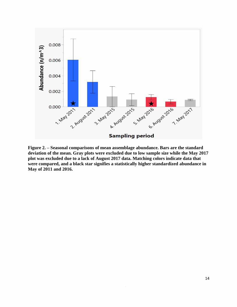
Data collected from 22,224 specimens were examined and only the most abundant

species, defined as those species that made up 99% of the total abundance in this study (Fine

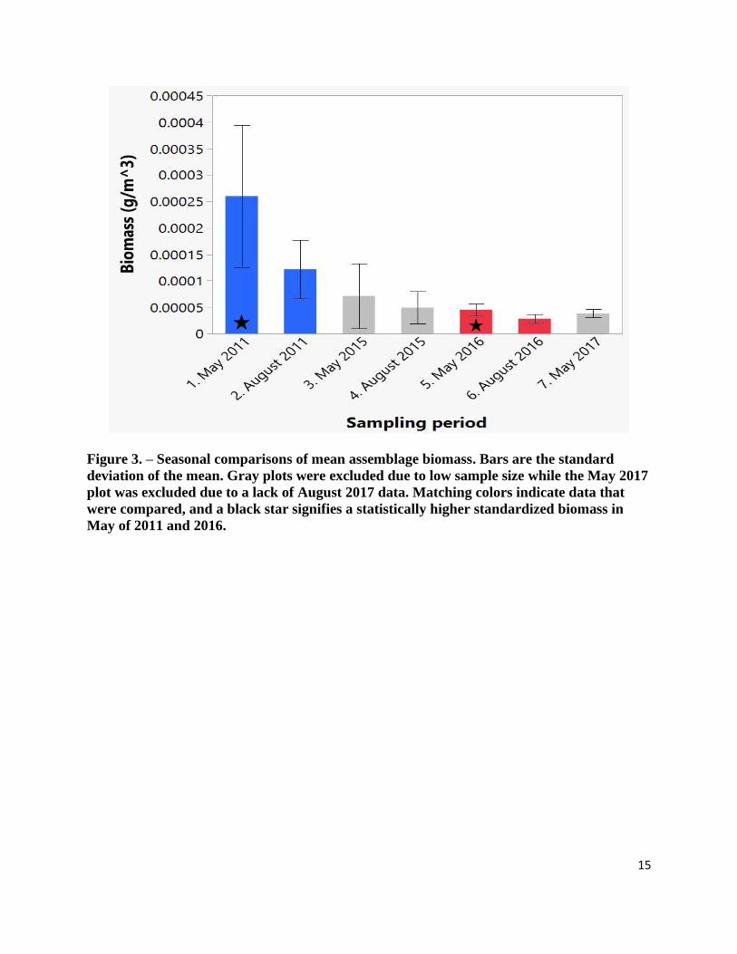
2016), were used for statistical analyses. A Kruskal-Wallis test indicated that significant

differences were present between the seasons, in terms of both abundance (χ2(3) = 24.785, p <

0.001) and biomass (χ2(3) = 25.246, p < 0.001). A post hoc multiple comparisons test showed

that abundance was significantly higher in May than in August for 2011 (Z = -2.248, p = 0.024)

and 2016 (Z = -2.388, p = 0.017). Biomass was also statistically higher in May for both 2011 (Z

= -2.396, p = 0.017) and 2016 (Z = -2.388, p = 0.017). The sample size for May and August 2015

samples were too small for statistical analysis, but as with the other years, there were more

euphausiids present in May than in August (Figure 2 & 3).

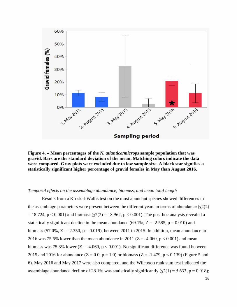
A total of 1,085 females bearing eggs (henceforth called gravid females) were identified,

and of these, 95% were Nematoscelis atlantica/microps. The remaining 5% were identified as

Euphausia gibboides, Nematoscelis tenella, Stylocheiron abbreviatum, Stylocheiron carinatum

and Stylocheiron maximum. Nematoscelis tenella gravid females (n=36) were all caught in

August 2011. Counts of other gravid females, identified as either Euphausia gibboides,

Stylocheiron abbreviatum, Stylocheiron carinatum and Stylocheiron maximum, ranged between 0

– 3 individuals each season. Such low numbers could not be included in the statistical analysis of

the seasonality of reproduction for each species considered gravid; the analysis was therefore

limited to Nematoscelis atlantica/microps. Individual specimens equal to, or larger than, the

length of the smallest gravid Nematoscelis atlantica/microps female (10.44 mm) were deemed

sexually mature. Results showed significant differences between May and August were present

(Kruskal-Wallis test, χ2(3) = 13.393, p = 0.004). The percentage of the sample population found

to be gravid in May 2011 was higher than the levels in August 2011, 11.3% and 8.2%,

respectively, however the post hoc analysis was inconclusive (Z = -1.918, p = 0.055). There was,

however, a statistically higher proportion of gravid females in May than August in 2016, 20.6%

vs. 11.1%, respectively, (Z = -2.270, p = 0.023, Figure 4). While the sample size from May and

August 2015 were too small for statistical analysis, there were substantially more gravid females

in May than in August, with both the maximum and minimum percentages found in this study

occurring in 2015 (32% and 2.5%, in May and August, respectively).

14

Figure 2. – Seasonal comparisons of mean assemblage abundance. Bars are the standard

deviation of the mean. Gray plots were excluded due to low sample size while the May 2017

plot was excluded due to a lack of August 2017 data. Matching colors indicate data that

were compared, and a black star signifies a statistically higher standardized abundance in

May of 2011 and 2016.

15

Figure 3. – Seasonal comparisons of mean assemblage biomass. Bars are the standard

deviation of the mean. Gray plots were excluded due to low sample size while the May 2017

plot was excluded due to a lack of August 2017 data. Matching colors indicate data that

were compared, and a black star signifies a statistically higher standardized biomass in

May of 2011 and 2016.

16

Figure 4. – Mean percentages of the N. atlantica/microps sample population that was

gravid. Bars are the standard deviation of the mean. Matching colors indicate the data

were compared. Gray plots were excluded due to low sample size. A black star signifies a

statistically significant higher percentage of gravid females in May than August 2016.

Temporal effects on the assemblage abundance, biomass, and mean total length

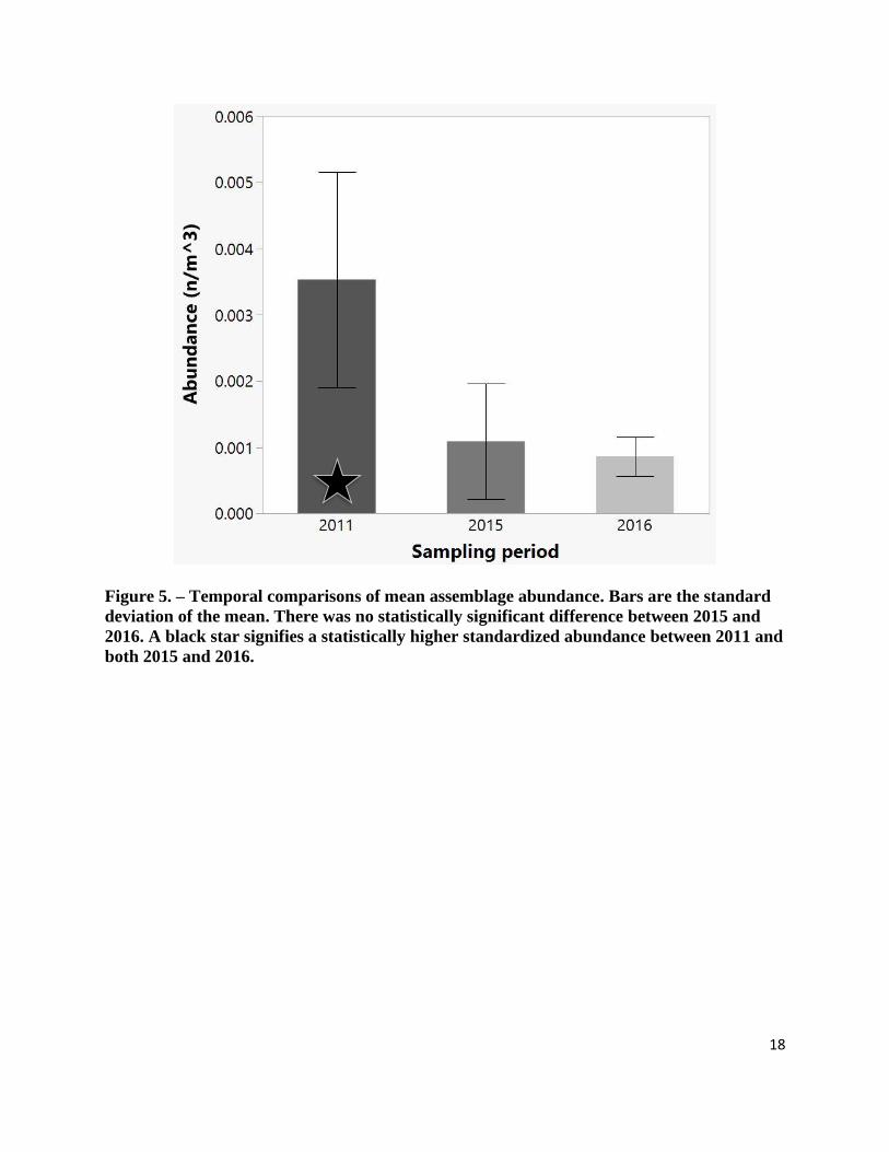
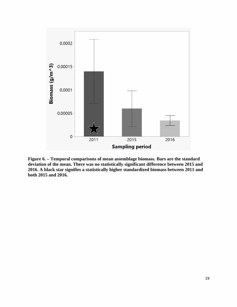
Results from a Kruskal-Wallis test on the most abundant species showed differences in

the assemblage parameters were present between the different years in terms of abundance (χ2(2)

= 18.724, p < 0.001) and biomass (χ2(2) = 18.962, p < 0.001). The post hoc analysis revealed a

statistically significant decline in the mean abundance (69.1%, Z = -2.585, p = 0.010) and

biomass (57.0%, Z = -2.350, p = 0.019), between 2011 to 2015. In addition, mean abundance in

2016 was 75.6% lower than the mean abundance in 2011 (Z = -4.060, p < 0.001) and mean

biomass was 75.3% lower (Z = -4.060, p < 0.001). No significant difference was found between

2015 and 2016 for abundance (Z = 0.0, p = 1.0) or biomass (Z = -1.479, p < 0.139) (Figure 5 and

6). May 2016 and May 2017 were also compared, and the Wilcoxon rank sum test indicated the

assemblage abundance decline of 28.1% was statistically significantly (χ2(1) = 5.633, p = 0.018);

17

biomass also declined by 14.7%, but this change was not statistically significant (χ2(2) = 1.20, p

= 0.273).

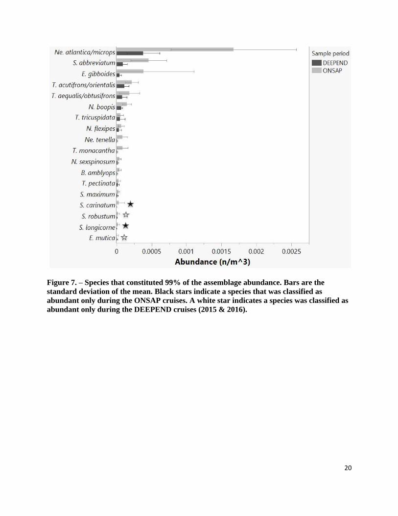
With no significant difference between 2015 and 2016, the two DEEPEND cruises were

then combined and treated as a single dataset and compared with the ONSAP data for individual

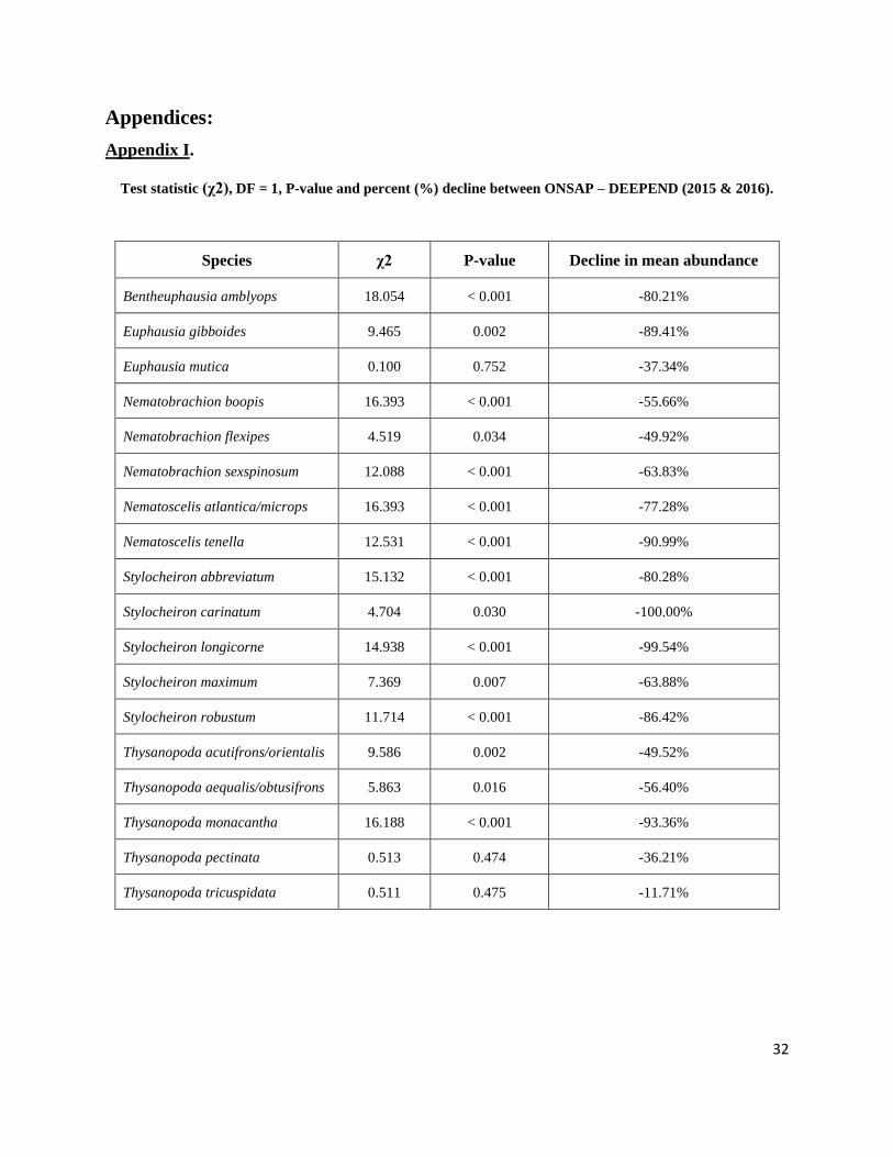
species comparisons. Every species defined as abundant experienced a decline between the

ONSAP and DEEPEND cruises and, for 15 of these species, this decline was statistically

significant in terms of at least one parameter (Appendix I.). Thysanopoda tricuspidata was the

only abundant species without significant changes, in abundance (Wilcoxon, χ2(1) = 0.511, p =

0.475) or biomass (Wilcoxon, χ2(1) = 0.2269, p = 0.634), while also remaining within the top

99% most abundant species throughout the ONSAP and DEEPEND cruises. Thysanopoda

tricuspidata was considered one of the nine most abundant taxa, meaning it was one of the few

species to be caught in abundance during every cruise. The most abundant species of this study,

Nematoscelis atlantica/microps accounted for nearly 47% of the entire assemblage abundance in

2011 and 37% in the 2015 – 2016 dataset, being four times more abundant than the 2nd most

abundant species, Euphausia gibboides. Like most species, Nematoscelis atlantica/microps

significantly decreased in abundance between 2011 to 2015 – 2016, by 77.3% (Wilcoxon, χ2(1)

= 16.393, p < 0.001) and biomass by 84.4% (Wilcoxon, χ2(1) = 15.756, p < 0.001), (Table 3).

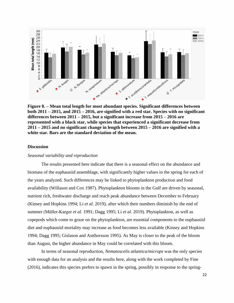
Assemblage mean total length (MTL) also declined significantly between ONSAP to DEEPEND

(Wilcoxon, χ2(1) = 18.842, p < 0.001) and changes between each year of sampling were only

examined for the most abundant taxa as they were the few species caught each year. All the most

abundant taxa showed the same trend: a decrease in MTL between 2011 – 2015, followed by an

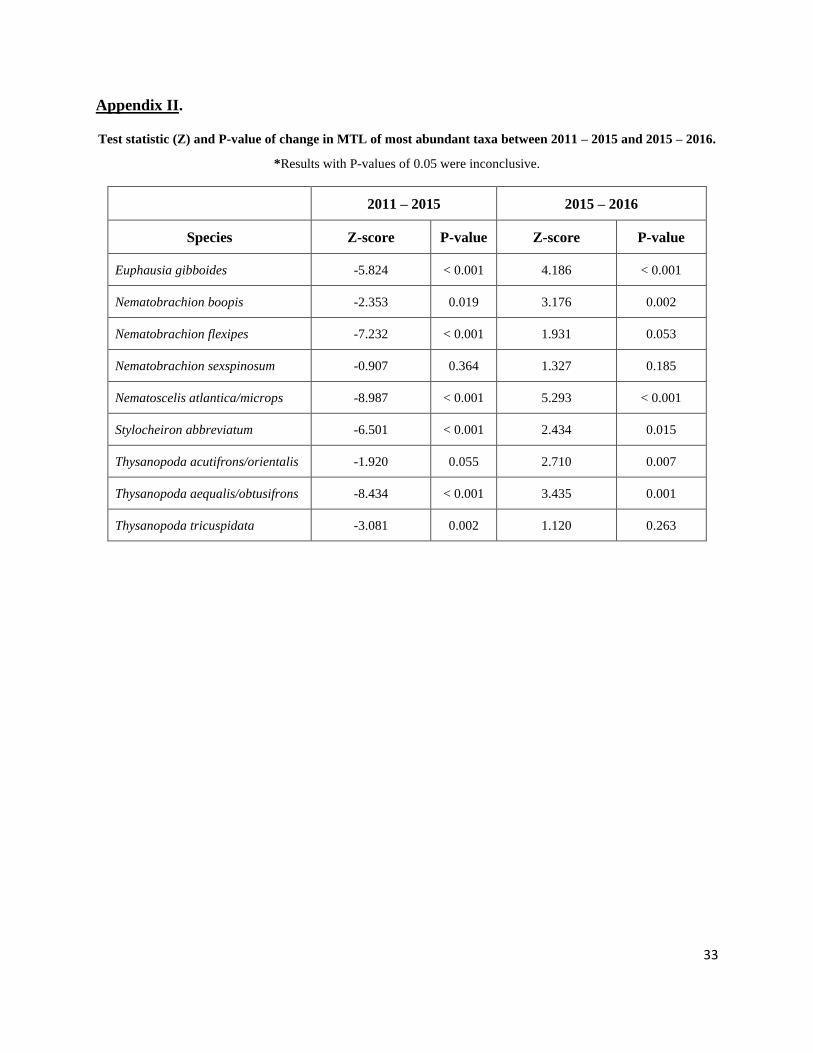
increase between 2015 – 2016 samples (Figure 8). A post hoc analysis showed that for seven out

of nine species, this decrease in MTL between 2011 – 2015 was highly significant, while

significant increases in MTL between 2015 – 2016 were apparent for six of the nine most

abundant taxa (Appendix II.). Nematobrachion sexspinosum was the only species that did not

show any significant changes in MTL (post hoc, Z = -0.907, p = 0.364, 2011 – 2015; Z = 1.327,

p = 0.185, 2015 – 2016).

18

Figure 5. – Temporal comparisons of mean assemblage abundance. Bars are the standard

deviation of the mean. There was no statistically significant difference between 2015 and

2016. A black star signifies a statistically higher standardized abundance between 2011 and

both 2015 and 2016.

19

Figure 6. – Temporal comparisons of mean assemblage biomass. Bars are the standard

deviation of the mean. There was no statistically significant difference between 2015 and

2016. A black star signifies a statistically higher standardized biomass between 2011 and

both 2015 and 2016.

20

Figure 7. – Species that constituted 99% of the assemblage abundance. Bars are the

standard deviation of the mean. Black stars indicate a species that was classified as

abundant only during the ONSAP cruises. A white star indicates a species was classified as

abundant only during the DEEPEND cruises (2015 & 2016).

21

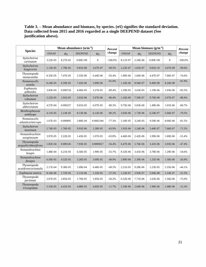
Table 3. – Mean abundance and biomass, by species. (σx̅) signifies the standard deviation.

Data collected from 2015 and 2016 regarded as a single DEEPEND dataset (See

justification above).

Species Mean abundance (n/m-3) Percent

change

Mean biomass (g/m-3) Percent

change ONSAP σx̅ DEEPEND σx̅ ONSAP σx̅ DEEPEND σx̅

Stylocheiron

carinatum 3.22E-05 8.27E-05 0.00E+00 0 -100.0% 8.11E-07 2.34E-06 0.00E+00 0 -100.0%

Stylocheiron

longicorne 2.15E-05 1.79E-05 9.81E-08 3.67E-07 -99.5% 2.22E-07 1.81E-07 9.81E-10 3.67E-09 -99.6%

Thysanopoda

monacantha 8.35E-05 7.47E-05 5.55E-06 6.44E-06 -93.4% 1.90E-06 1.84E-06 4.47E-07 7.06E-07 -74.6%

Nematoscelis

tenella 8.24E-05 6.59E-05 7.42E-06 5.89E-06

-91.0% 1.16E-06 8.94E-07 9.40E-08 8.24E-08

-91.9%

Euphausia

gibboides 3.83E-04 0.000724 4.06E-05 3.27E-05 -89.4% 1.59E-05 3.63E-05 1.19E-06 1.03E-06 -92.5%

Stylocheiron

robustum 2.22E-05 1.91E-05 3.01E-06 5.97E-06 -86.4% 1.16E-06 7.50E-07 9.76E-08 2.07E-07 -88.4%

Stylocheiron

abbreviatum 4.57E-04 0.000257 9.01E-05 6.07E-05 -80.3% 9.75E-06 5.83E-06 1.49E-06 1.01E-06 -84.7%

Bentheuphausia

amblyops 4.11E-05 2.13E-05 8.13E-06 6.12E-06 -80.2% 3.05E-06 1.73E-06 6.24E-07 5.06E-07 -79.5%

Nematoscelis

atlantica/microps 1.67E-03 0.000895 3.80E-04 0.0002344 -77.3% 5.18E-05 3.24E-05 9.59E-06 8.06E-06 -81.5%

Stylocheiron

maximum 2.74E-05 1.76E-05 9.91E-06 1.28E-05 -63.9% 1.91E-06 1.24E-06 5.44E-07 7.66E-07 -71.5%

Nematobrachion

sexspinosum 3.97E-05 2.22E-05 1.43E-05 1.07E-05 -63.8% 4.46E-06 2.42E-06 1.99E-06 1.69E-06 -55.4%

Thysanopoda

aequalis/obtusifrons 1.82E-04 0.000145 7.93E-05 0.0000657 -56.4% 6.47E-06 5.76E-06 3.41E-06 3.03E-06 -47.4%

Nematobrachion

boopis 1.48E-04 6.21E-05 6.56E-05 1.90E-05 -55.7% 8.32E-06 3.41E-06 3.78E-06 1.29E-06 -54.6%

Nematobrachion

flexipes 6.50E-05 4.52E-05 3.26E-05 3.69E-05 -49.9% 2.89E-06 2.39E-06 1.25E-06 1.50E-06 -56.9%

Thysanopoda

acutifrons/orientalis 2.17E-04 9.38E-05 1.09E-04 6.48E-05 -49.5% 2.21E-05 9.28E-06 1.23E-05 5.35E-06 -44.1%

Euphausia mutica 8.16E-06 1.72E-05 5.11E-06 1.22E-05 -37.3% 1.23E-07 2.93E-07 5.94E-08 1.33E-07 -51.5%

Thysanopoda

pectinata 2.67E-05 2.85E-05 1.70E-05 1.85E-05 -36.2% 6.52E-06 7.71E-06 1.63E-06 1.56E-06 -75.0%

Thysanopoda

tricuspidata 5.53E-05 4.41E-05 4.88E-05 6.85E-05 -11.7% 2.16E-06 2.04E-06 1.90E-06 2.48E-06 -12.3%

22

Figure 8. – Mean total length for most abundant species. Significant differences between

both 2011 – 2015, and 2015 – 2016, are signified with a red star. Species with no significant

differences between 2011 – 2015, but a significant increase from 2015 – 2016 are

represented with a black star, while species that experienced a significant decrease from

2011 – 2015 and no significant change in length between 2015 – 2016 are signified with a

white star. Bars are the standard deviation of the mean.

Discussion

Seasonal variability and reproduction

The results presented here indicate that there is a seasonal effect on the abundance and

biomass of the euphausiid assemblage, with significantly higher values in the spring for each of

the years analyzed. Such differences may be linked to phytoplankton production and food

availability (Willason and Cox 1987). Phytoplankton blooms in the Gulf are driven by seasonal,

nutrient rich, freshwater discharge and reach peak abundance between December to February

(Kinsey and Hopkins 1994; Li et al. 2019), after which their numbers diminish by the end of

summer (Müller‐Karger et al. 1991; Dagg 1995; Li et al. 2019). Phytoplankton, as well as

copepods which come to graze on the phytoplankton, are essential components to the euphausiid

diet and euphausiid mortality may increase as food becomes less available (Kinsey and Hopkins

1994; Dagg 1995; Gislason and Astthorsson 1995). As May is closer to the peak of the bloom

than August, the higher abundance in May could be correlated with this bloom.

In terms of seasonal reproduction, Nematoscelis atlantica/microps was the only species

with enough data for an analysis and the results here, along with the work completed by Fine

(2016), indicates this species prefers to spawn in the spring, possibly in response to the spring-

23

time bloom. Euphausiid reproduction is complicated because it varies by species, and even

among members of the same species, so it is difficult to make predictions about how often a

species reproduces in a region where little data are available (Mauchline and Fisher 1969; Siegel

2000). For example, Thysanopoda acutifrons are only known to breed in May within the North

Atlantic, while for Meganyctiphanes norvegica, breeding varies with latitude in this region

(Einarsson 1945). These differences in breeding preferences may due to the timing, duration and

magnitude of phytoplankton blooms around the world, events which have been observed to

coincide with euphausiid spawning times (Pillar and Stuart 1988; Dalpadado and Skjoldal 1996;

Nicol and Endo 1997). All euphausiids within the GOM are either tropical or subtropical species

and may reproduce seasonally as peak phytoplankton production in the GOM occurs earlier in

the year. No conclusions regarding the preferred spawning time of the remaining 17 species

could be made due to either low numbers or a complete lack of gravid females.

Temporal changes in the assemblage

Species were considered abundant if they constituted 99% of the total assemblage

abundance and rare if they were in the remaining 1% (Fine 2016). In May 2011 alone (from the

MS7 samples), of the 27 species collected over the course of this study, 13 species were

considered abundant while 14 were either absent from this sample period (meaning that they

were present in the subsequent samples) or considered rare. Fine (2016), which included all three

months of MS7 sample collections, listed 16 species as abundant and 15 rare. Euphausia mutica,

Stylocheiron elongatum and Stylocheiron maximum, considered abundant in Fine (2016), were

rare species in May 2011 from the work presented here. This apparent disparity is the result of

our slightly divergent methodologies for selecting data for analyses. The euphausiid individuals

collected for Fine (2016) came from samples collected between April – June 2011 with samples

depths ranging from 0 – 1500 m, whereas the analysis presented here used data solely from May

of the MS7 cruise and depths of 0 – 1000 m (see justification in methods).

Although significant declines in the assemblage abundance and biomass occurred

between 2011, one year after the oil spill, and 2015 – 2016, five to six years after the oil spill,

they cannot be directly attributed to the DWHOS. Since there were no pre-spill data on the

assemblage available, it is difficult to assess whether the decline is part of normal biological

variability or is a direct result of the spill. It should be noted, however, that large scale die-offs of

24

zooplankton, which included larval stage euphausiids, occurred following the 1979 Ixtoc-1 oil

spill, which released 3.1 million barrels of oil into the shelf waters of the southern GOM. After

this spill, there was a reduction in biomass by a factor of four, relative to pre-spill levels (Próo et

al. 1986). Some species of euphausiids have displayed limited swimming capacity, impaired

feeding ability and increased mortality due to prolonged exposure to dissolved hydrocarbons

under laboratory conditions (Arnberg et al. 2017; Knap et al. 2017). Knap et al. (2017) also

showed that, of all the crustaceans tested, euphausiids were among the most sensitive to the

toxicity of the hydrocarbon used in that study. Although it’s uncertain how long the oil from the

DWHOS was in contact with the euphausiid assemblage in the GOM, computer modelling

results indicated it could have taken at least 100 days before more than 50% of the oil exited the

model’s domain extent (Weisberg et al. 2011). Laboratory results showed it only took 24-hours

of exposure time to reach a lethal concentration of the hydrocarbon 1-methylnaphthalene and

prompt mortality in several euphausiid species (Knap et al. 2017).

In addition, copepods and phytoplankton, common constituents of the euphausiid diet,

may have also experienced a decline in their abundance from the effects of the DWHOS. In

2012, 2 years after the spill, laboratory results on samples taken from near-shore GOM locations

indicated that mesozooplankton (mostly comprised of copepods) mortality peaked at 96% and

was found to increase with oil concentration (Almeda et al. 2013). In addition, satellite data from

2001 to 2017 on Chlorophyll-a (Chl-a) concentration in the GOM, a proxy for the level of

primary productivity, noted a substantial decrease in 2011 which remained low until 2014,

relative to pre-spill years. Chl-a then returned to pre-spill values in 2015 (Li et al. 2019). This

appears to coincide with the change in MTL of the most abundant taxa observed in this study; a

significant decline occurred between 2011 to 2015 and was followed by an increase in MTL

which, in some species, exceeded 2011 values. It may be possible that, as their food source

became scarcer, the carrying capacity of that region could no longer support larger individuals,

but once phytoplankton density values increased, larger individuals could once again be

supported.

Although MTL increased, both assemblage abundance and biomass declined through

2016 despite a renewal of a major source of food. This continued downward trend between May

2016 and May 2017 may relate to a maximum sustainable yield (MSY). This is a term used in

fisheries science and is the theorized limit of exploitation for a commercially viable population

25

of fish. Once this limit is exceeded, the number of reproductive individuals in the population is

not high enough to replace the individuals that have been removed, meaning that the population

cannot sustain itself, and the associated fishery then crashes. The Orange Roughy (Hoplostethus

atlanticus) is a commercially harvested deep-sea fish that is vulnerable to overexploitation, in-

part due to its low fecundity, a common trait among many deep-sea species (Koslow et al. 2000;

Lack et al. 2003). Due to its high vulnerability, for Hoplostethus atlanticus the MSY is

removable of 30% of the biomass; beyond this point the assemblage population is no longer be

considered sustainable. Given that the euphausiid assemblage declined by nearly 76% between

2011 and 2016, and continued to decline into 2017, it may too have reached a point in its

biomass levels where the return to a more stable assemblage population is uncertain. All

euphausiids within the GOM are tropical and sub-tropical species, which means they have

relatively low fecundity, or egg count, especially when compared to the Antarctic euphausiid

species, Euphausia superba, which possess between 310 – 800 eggs per female (Mauchline and

Fisher 1969; Mauchline 1980; Kinsey and Hopkins 1994). Estimates for some species found in

the GOM rarely exceed 100 eggs per female (Roger 1976; Mauchline 1980). Koslow et al.

(2000) also surmises low fecundity may dampen the resiliency of a species. For example,

Stylocheiron carinatum and Stylocheiron longicorne experienced significant declines between

2011 and 2015, so much so that Stylocheiron longicorne was rarely caught in DEEPEND

samples, while Stylocheiron carinatum was never observed again after May 2011. Both species

of this genus are estimated to have no more than 16 eggs per female (Roger 1976). In contrast,

Thysanopoda tricuspidata, a species with similar abundance levels as the two Stylocheiron

species in 2011, did not experience a statistically significant decline in abundance or biomass

and, and this species carried hundreds of eggs. Euphausiid species with higher fecundity may be

more resilient to significant reductions in their abundance than those with lower fecundity.

Therefore, the effects of intrinsically low fecundity, an intermittent lack of food and likely

exposure to hydrocarbon compounds in the water column, may all be important factors to

consider when attempting to determine the causes of the decline observed in the euphausiid

assemblage of the northern GOM, following the DWHOS.

The full consequences of this decline to the ecology of the Gulf are unknown; however,

analogies may be drawn from a computer model that simulated the over exploitation of

euphausiids off the coast of California (Kaplan et al. 2013). Their results indicated that

26

predators, specifically various species of fish and whales, experienced declines of near 20%. In

the GOM, a significant decline occurred amongst the myctophids and gonostomatids (Sutton et

al. in review), which specialize on krill (Hopkins et al. 1996) and would likely experience

significant impacts from the decline in the euphausiids. Other species which rely on euphausiids

as a food source may have also experienced significant declines, but more study is needed.

Conclusions

The results from this study on the euphausiid assemblage in the northern GOM revealed a

significant reduction in abundance and biomass between 2011 to 2015 – 2016, along with a

continuation of this decline into May 2017. Although these findings could not be directly

attributed to the DWHOS due to a lack of information prior to the spill, the data collected for this

thesis did give insight into how the assemblage fluctuated years after a major oil spill. The

statistically significant decline in abundance between May 2016 to May 2017 suggests that the

euphausiid assemblage of the northern GOM may have been reduced to such an extent that a rise

in their numbers may take many years. Seasonality, particularly as it relates to food availability,

was also identified as an important factor to include in any temporal analysis on the euphausiid

assemblage. It likely affects the reproductive cycle of many euphausiid species, including the

most abundant species in this study, Nematoscelis atlantica/microps. These results presented

here add some empirical support to the hypothesis that the initial change in the euphausiid

assemblage between 2011 – 2015 was due to an acute stressor such as an oil spill, rather than

normal temporal variability in the assemblage.

27

References

Abbriano RM, Carranza MM, Hogle SL, Levin RA, Netburn AN, Seto KL, Snyder SM, Franks

PJ. 2011. Deepwater horizon oil spill: A review of the planktonic response.

Oceanography. 24(3):294-301.

Almeda R, Wambaugh Z, Wang Z, Hyatt C, Liu Z, Buskey E. 2013. Interactions between

zooplankton and crude oil: Toxic effects and bioaccumulation of polycyclic aromatic

hydrocarbons. PloS one. 8(6):e67212.

Arnberg M, Moodley L, Dunaevskaya E, Ramanand S, Ingvarsdóttir A, Nilsen M, Ravagnan E,

Westerlund S, Sanni S, Tarling GA. 2017. Effects of chronic crude oil exposure on early

developmental stages of the northern krill (meganyctiphanes norvegica). Journal of

Toxicology and Environmental Health, Part A. 80(16-18):916-931.

Baker A, Boden B, Brinton E. 1990. A practical guide to the euphausiids of the world. British

Museum (Natural History), London: Natural History Museum Publications.

Bradshaw C, Hindell M, Best N, Phillips K, Wilson G, Nichols P. 2003. You are what you eat:

Describing the foraging ecology of southern elephant seals (mirounga leonina) using

blubber fatty acids. Proceedings of the Royal Society of London B: Biological Sciences.

270(1521):1283–1292.

Brinton E. 1962. The distribution of pacific euphausiids. Scripps Institution of Oceanography.

8(2):51-269.

Brinton E, Ohman M, Townsend A, Knight M, Breidgeman A. 1999. Euphausiids of the world

ocean (world biodiversity database cd-rom series). Eti expert center for taxonomic

identification. New York: Springer-Verlag.

Burdett EA, Fine CD, Sutton TT, Cook AB, Frank TM. 2017. Geographic and depth

distributions, ontogeny, and reproductive seasonality of decapod shrimps (caridea:

Oplophoridae) from the northeastern gulf of mexico. Bulletin of Marine Science.

93(3):743-767.

Carassou L, Hernandez F, Graham W. 2014. Change and recovery of coastal mesozooplankton

community structure during the deepwater horizon oil spill. Environmental Research

Letters. 9(12):12.

Cargnelli L, Griesbach S, Zetlin C. 1999. Essential fish habitat source document: Northern

shortfin squid, illex illecebrosus, life history and habitat characteristics. NOAA technical

memorandum NMFS-NE. 147:21.

28

Castellanos IA, Morales ES-. 2009. Euphausiacea (crustacea) of the gulf of mexico. In: Felder

DL, Camp DK, editors. Gulf of mexico origin, waters, and biota : Biodiversity. College

Station, UNITED STATES: Texas A&M University Press. p. pp 1013-1018.

Dagg M. 1995. Copepod grazing and the fate of phytoplankton in the northern gulf of mexico.

Continental Shelf Research. 15(11-12):1303-1317.

Dalpadado P, Skjoldal HR. 1996. Abundance, maturity and growth of the krill species

thysanoessa inermis and t. Longicaudata in the barents sea. Marine Ecology Progress

Series. 144:175-183.

Deagle B, Gales N, Evans K, Jarman S, Robinson S, Trebilco R, Hindell M. 2007. Studying

seabird diet through genetic analysis of faeces: A case study on macaroni penguins

(eudyptes chrysolophus). PLoS One. 2(9):e831.

Einarsson H. 1945. Euphausiacea, northern atlantic species. Copenhagen, Denmark: Dana

Report. p. 1-191.

Everitt B, Skrondal A. 2010. The cambridge dictionary of statistics. 4th ed. Cambridge, U.K.:

Cambridge University Press Cambridge. p. 353.

Felder DL, Camp DK. 2009. Gulf of mexico origin, waters, and biota: Biodiversity. Texas A&M

University Press.

Fine C. 2016. The vertical and horizontal distribution of deep-sea crustaceans of the order

euphausiacea (malacostraca: Eucarida) from the northern gulf of mexico with notes on

reproductive seasonality. Nova Southeastern University.

Frank T, Fine CD, Burdett EA, Cook AB, Sutton TT. 2020. The vertical and horizontal

distribution of deep-sea crustaceans in the order euphausiacea in the vicinity of the

deepwater horizon oil spill. Frontiers in Marine Science. 7:99.

French-McCay D, Graham E, Schroeder M, Sutton T. 2011. Nrda 10-meter mocness spring 2011

plankton sampling cruise plan.

Gasca R, Castellanos I, Biggs D. 2001. Euphausiids (crustacea, euphausiacea) and summer

mesoscale features in the gulf of mexico. Bulletin of Marine Science. 68(3):397-408.

Gislason A, Astthorsson OS. 1995. Seasonal cycle of zooplankton southwest of iceland. Journal

of Plankton Research. 17(10):1959-1976.

29

Hopkins TL, Sutton TT, Lancraft TM. 1996. The trophic structure and predation impact of a low

latitude midwater fish assemblage. Progress in Oceanography. 38(3):205-239.

Ikeda T. 1985. Life history of antarctic krill euphausia superba: A new look from an

experimental approach. Bulletin of Marine Science. 37(2):599-608.

Jayalakshmi K, Jasmine P, Muraleedharan K, Prabhakaran M, Habeebrehman H, Jacob J,

Achuthankutty C. 2011. Aggregation of euphausia sibogae during summer monsoon

along the southwest coast of india. Journal of Marine Biology. 2011:12.

Kaplan I, Brown C, Fulton E, Gray I, Field J, Smith A. 2013. Impacts of depleting forage species

in the california current. Environmental Conservation. 40(04):380-393.

Kinsey S, Hopkins T. 1994. Trophic strategies of euphausiids in a low-latitude ecosystem.

Marine Biology. 118(4):651–661.

Knap A, Turner NR, Bera G, Renegar DA, Frank T, Sericano J, Riegl BM. 2017. Short‐term

toxicity of 1‐methylnaphthalene to americamysis bahia and 5 deep‐sea crustaceans.

Environmental toxicology and chemistry. 36(12):3415-3423.

Koslow JA, Boehlert G, Gordon J, Haedrich R, Lorance P, Parin N. 2000. Continental slope and

deep-sea fisheries: Implications for a fragile ecosystem. ICES Journal of Marine Science.

57(3):548-557.

Lack M, Oceania T, Short K, Willock A. 2003. Managing risk and uncertainty in deep-sea

fisheries: Lessons from orange roughy.

Li Y, Hu C, Quigg A, Gao H. 2019. Potential influence of the deepwater horizon oil spill on

phytoplankton primary productivity in the northern gulf of mexico. Environmental

Research Letters.

Mackintosh N. 1972. Life cycle of antarctic krill in relation to ice and water conditions.

Cambridge University Press. p. 94.

Mauchline J. 1980. The biology of euphausiids. Advances in marine biology. 18:373-623.

Mauchline J, Fisher L. 1969. Advances in marine biology. London, U.K. and New York, U.S.A.:

Academic Press.

McDonald JH. 2009. Handbook of biological statistics. sparky house publishing Baltimore, MD.

30

McNutt MK, Camilli R, Crone TJ, Guthrie GD, Hsieh PA, Ryerson TB, Savas O, Shaffer F.

2012. Review of flow rate estimates of the deepwater horizon oil spill. Proceedings of the

National Academy of Sciences. 109(50):20260-20267.

Müller‐Karger FE, Walsh JJ, Evans RH, Meyers MB. 1991. On the seasonal phytoplankton

concentration and sea surface temperature cycles of the gulf of mexico as determined by

satellites. Journal of Geophysical Research: Oceans. 96(C7):12645-12665.

Nichols D. 2018. A temporal analysis of a deep-pelagic crustacean assemblage (decapoda:

Caridea: Oplophoridae and pandalidae) in the gulf of mexico after the deepwater horizon

oil spill. Nova Southeastern University.

Nicol S, Endo Y. 1997. Krill fisheries of the world. Food & Agriculture Org.

Nicol S, Endo Y. 1999. Krill fisheries: Development, management and ecosystem implications.

Aquatic Living Resources. 12(2):105-120.

Öztuna D, Elhan AH, Tüccar E. 2006. Investigation of four different normality tests in terms of

type 1 error rate and power under different distributions. Turkish Journal of Medical

Sciences. 36(3):171-176.

Pillar S, Stuart V. 1988. Population structure, reproductive biology and maintenance of

euphausia lucens in the southern benguela current. Journal of Plankton Research.

10(6):1083-1098.

Próo SGd, Chávez E, Alatriste F, De La Campa S, De la Cruz G, Gómez L, Guadarrama R,

Guerra A, Mille S, Torruco D. 1986. The impact of the ixtoc-1 oil spill on zooplankton.

Journal of plankton Research. 8(3):557-581.

Robinson C. 2000. The consumption of euphausiids by the pelagic fish community off

southwestern vancouver island, british columbia. Journal of Plankton Research.

22(9):1649-1662.

Roger C. 1976. Fecundity of tropical euphausiids from the central and western pacific ocean.

Crustaceana. 31(1):103-105.

Rooker JR, Kitchens LL, Dance MA, Wells RD, Falterman B, Cornic M. 2013. Spatial,

temporal, and habitat-related variation in abundance of pelagic fishes in the gulf of

mexico: Potential implications of the deepwater horizon oil spill. PloS one. 8(10):e76080.

Schoenherr J. 1991. Blue whales feeding on high concentrations of euphausiids around monterey

submarine canyon. Canadian Journal of Zoology. 69(3):583-594.

31

Siegel V. 2000. Krill (euphausiacea) life history and aspects of population dynamics. Canadian

Journal of Fisheries and Aquatic Sciences. 57(S3):130-150.

Simard Y, Ladurantaye R, Therriault J. 1986. Aggregation of euphausiids along a coastal shelf in

an upwelling environment. Marine Ecology Progress Series. 32(20):203-215.

Strickland J, Khailov K, Finenko Z, McIntyre A, Munro A, Zaika V, Qasim S, Marhsall N. 1970.

Marine food chains. Edinburgh, Great Britain: Univerity of California Press. p. 244 - 245.

Weisberg RH, Zheng L, Liu Y. 2011. Tracking subsurface oil in the aftermath of the deepwater

horizon well blowout. Geophys Monogr Ser. 195:205-215.

Wiebe P, Morton A, Bradley A, Backus R, Craddock J, Barber V, Cowles T, Flierl G. 1985. New

development in the mocness, an apparatus for sampling zooplankton and micronekton.

Marine Biology. 87(3):313–323.

Willason SW, Cox JL. 1987. Diel feeding, laminarinase activity, and phytoplankton consumption

by euphausiids. Biological Oceanography. 4(1):1-24.

32

Appendices:

Appendix I.

Test statistic (χ2), DF = 1, P-value and percent (%) decline between ONSAP – DEEPEND (2015 & 2016).

Species χ2 P-value Decline in mean abundance

Bentheuphausia amblyops 18.054 < 0.001 -80.21%

Euphausia gibboides 9.465 0.002 -89.41%

Euphausia mutica 0.100 0.752 -37.34%

Nematobrachion boopis 16.393 < 0.001 -55.66%

Nematobrachion flexipes 4.519 0.034 -49.92%

Nematobrachion sexspinosum 12.088 < 0.001 -63.83%

Nematoscelis atlantica/microps 16.393 < 0.001 -77.28%

Nematoscelis tenella 12.531 < 0.001 -90.99%

Stylocheiron abbreviatum 15.132 < 0.001 -80.28%

Stylocheiron carinatum 4.704 0.030 -100.00%

Stylocheiron longicorne 14.938 < 0.001 -99.54%

Stylocheiron maximum 7.369 0.007 -63.88%

Stylocheiron robustum 11.714 < 0.001 -86.42%

Thysanopoda acutifrons/orientalis 9.586 0.002 -49.52%

Thysanopoda aequalis/obtusifrons 5.863 0.016 -56.40%

Thysanopoda monacantha 16.188 < 0.001 -93.36%

Thysanopoda pectinata 0.513 0.474 -36.21%

Thysanopoda tricuspidata 0.511 0.475 -11.71%

33

Appendix II.

Test statistic (Z) and P-value of change in MTL of most abundant taxa between 2011 – 2015 and 2015 – 2016.

*Results with P-values of 0.05 were inconclusive.

2011 – 2015 2015 – 2016

Species Z-score P-value Z-score P-value

Euphausia gibboides -5.824 < 0.001 4.186 < 0.001

Nematobrachion boopis -2.353 0.019 3.176 0.002

Nematobrachion flexipes -7.232 < 0.001 1.931 0.053

Nematobrachion sexspinosum -0.907 0.364 1.327 0.185

Nematoscelis atlantica/microps -8.987 < 0.001 5.293 < 0.001

Stylocheiron abbreviatum -6.501 < 0.001 2.434 0.015

Thysanopoda acutifrons/orientalis -1.920 0.055 2.710 0.007

Thysanopoda aequalis/obtusifrons -8.434 < 0.001 3.435 0.001

Thysanopoda tricuspidata -3.081 0.002 1.120 0.263

34

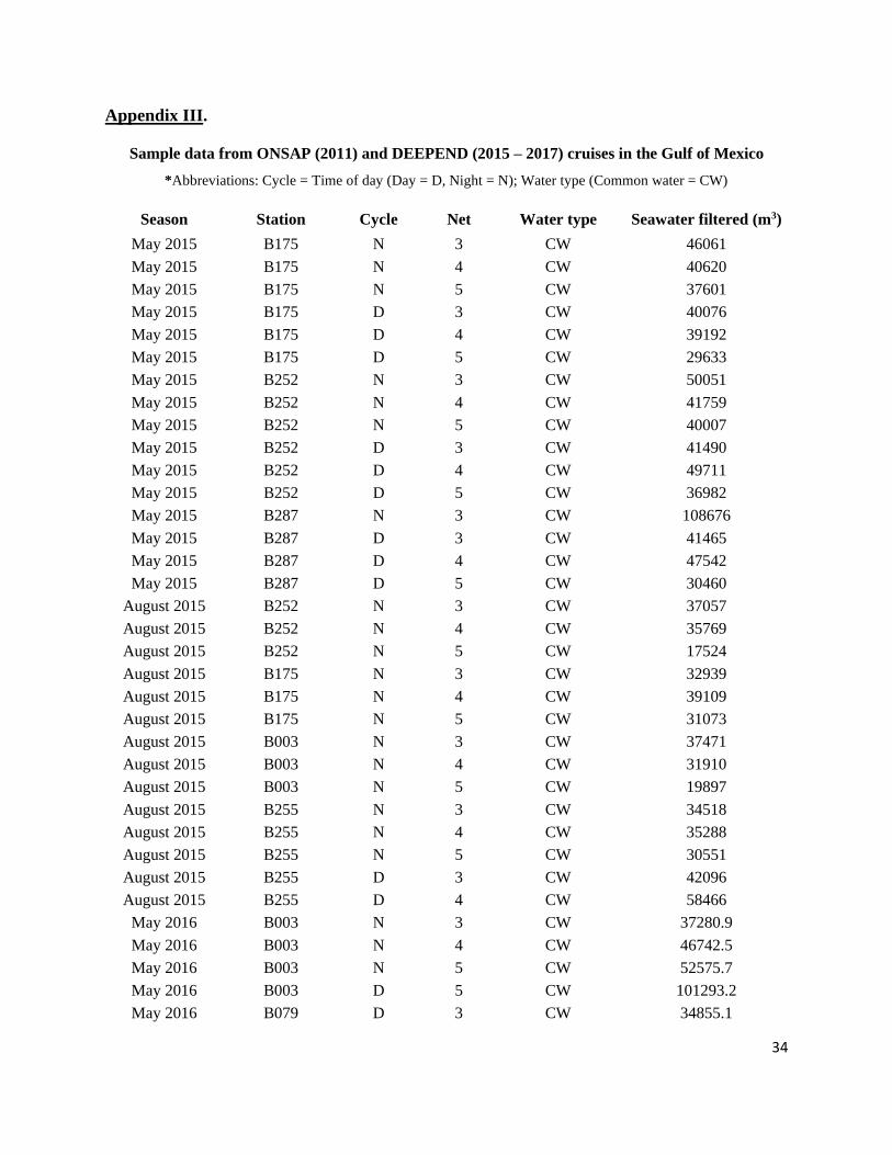
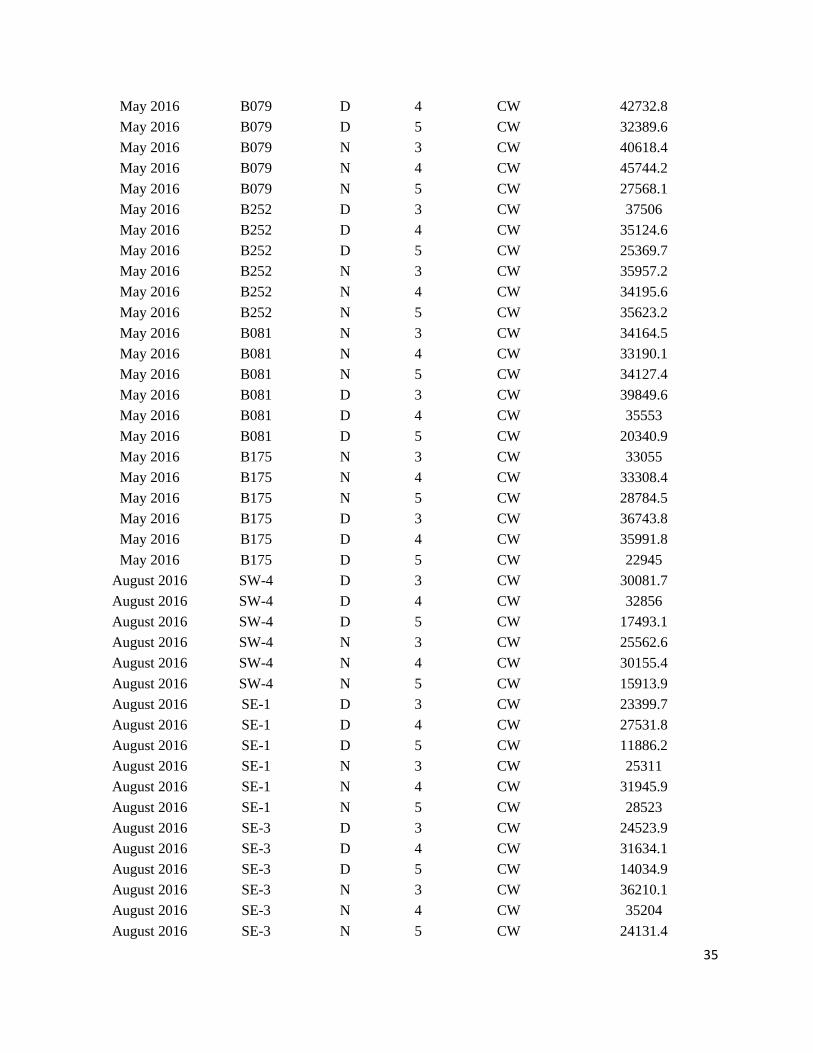
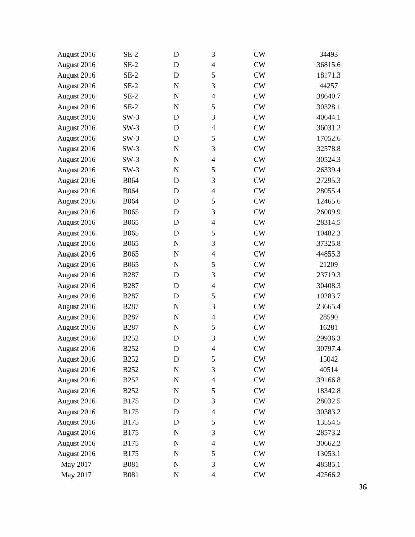
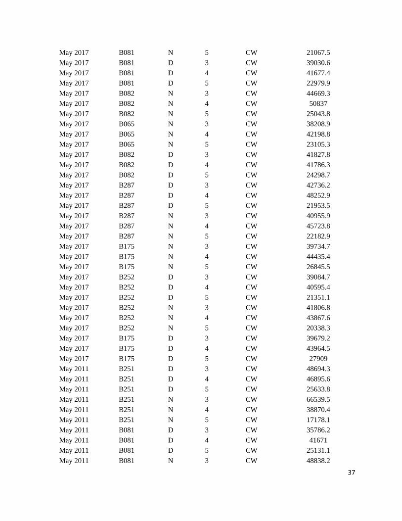
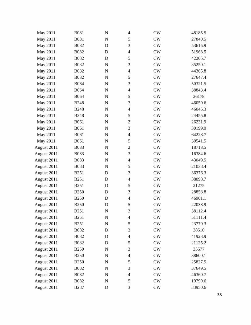
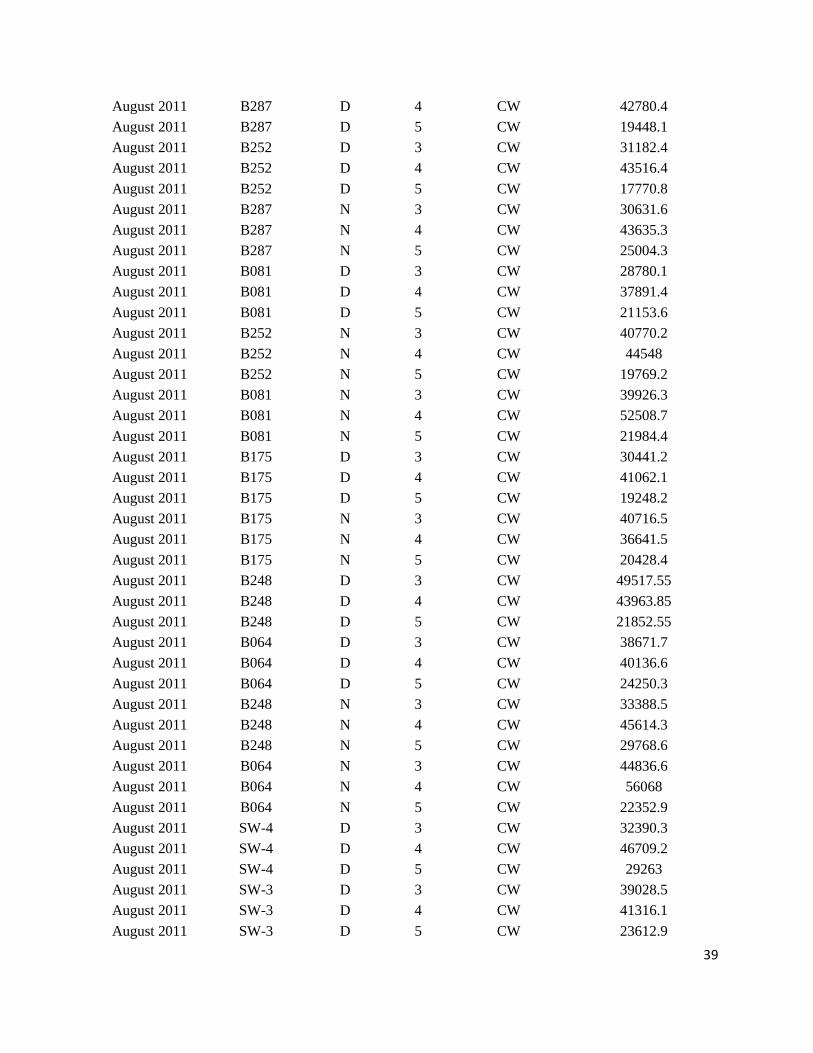
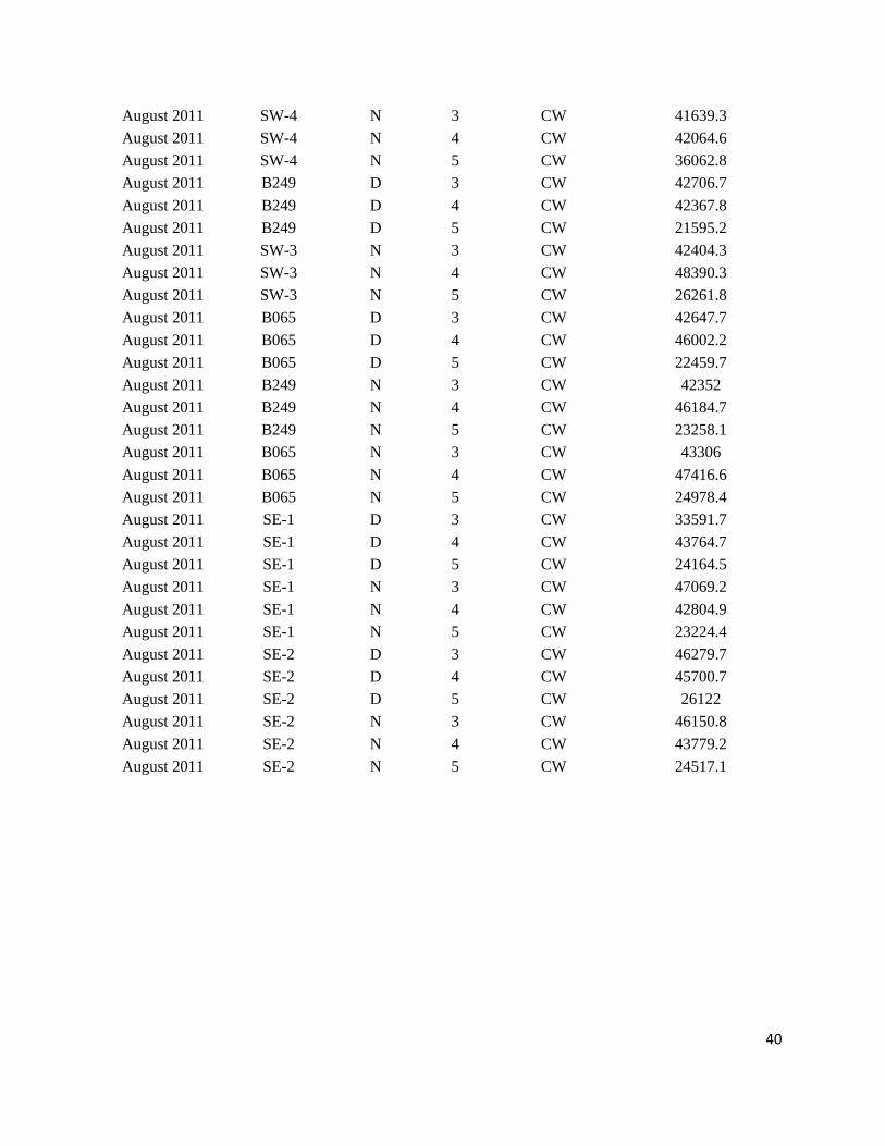
Appendix III.

Sample data from ONSAP (2011) and DEEPEND (2015 – 2017) cruises in the Gulf of Mexico

*Abbreviations: Cycle = Time of day (Day = D, Night = N); Water type (Common water = CW)

Season Station Cycle Net Water type Seawater filtered (m3)

May 2015 B175 N 3 CW 46061

May 2015 B175 N 4 CW 40620

May 2015 B175 N 5 CW 37601

May 2015 B175 D 3 CW 40076

May 2015 B175 D 4 CW 39192

May 2015 B175 D 5 CW 29633

May 2015 B252 N 3 CW 50051

May 2015 B252 N 4 CW 41759

May 2015 B252 N 5 CW 40007

May 2015 B252 D 3 CW 41490

May 2015 B252 D 4 CW 49711

May 2015 B252 D 5 CW 36982

May 2015 B287 N 3 CW 108676

May 2015 B287 D 3 CW 41465

May 2015 B287 D 4 CW 47542

May 2015 B287 D 5 CW 30460

August 2015 B252 N 3 CW 37057

August 2015 B252 N 4 CW 35769

August 2015 B252 N 5 CW 17524

August 2015 B175 N 3 CW 32939

August 2015 B175 N 4 CW 39109

August 2015 B175 N 5 CW 31073

August 2015 B003 N 3 CW 37471

August 2015 B003 N 4 CW 31910

August 2015 B003 N 5 CW 19897

August 2015 B255 N 3 CW 34518

August 2015 B255 N 4 CW 35288

August 2015 B255 N 5 CW 30551

August 2015 B255 D 3 CW 42096

August 2015 B255 D 4 CW 58466

May 2016 B003 N 3 CW 37280.9

May 2016 B003 N 4 CW 46742.5

May 2016 B003 N 5 CW 52575.7

May 2016 B003 D 5 CW 101293.2

May 2016 B079 D 3 CW 34855.1

35

May 2016 B079 D 4 CW 42732.8

May 2016 B079 D 5 CW 32389.6

May 2016 B079 N 3 CW 40618.4

May 2016 B079 N 4 CW 45744.2

May 2016 B079 N 5 CW 27568.1

May 2016 B252 D 3 CW 37506

May 2016 B252 D 4 CW 35124.6

May 2016 B252 D 5 CW 25369.7

May 2016 B252 N 3 CW 35957.2

May 2016 B252 N 4 CW 34195.6

May 2016 B252 N 5 CW 35623.2

May 2016 B081 N 3 CW 34164.5

May 2016 B081 N 4 CW 33190.1

May 2016 B081 N 5 CW 34127.4

May 2016 B081 D 3 CW 39849.6

May 2016 B081 D 4 CW 35553

May 2016 B081 D 5 CW 20340.9

May 2016 B175 N 3 CW 33055

May 2016 B175 N 4 CW 33308.4

May 2016 B175 N 5 CW 28784.5

May 2016 B175 D 3 CW 36743.8

May 2016 B175 D 4 CW 35991.8

May 2016 B175 D 5 CW 22945

August 2016 SW-4 D 3 CW 30081.7

August 2016 SW-4 D 4 CW 32856

August 2016 SW-4 D 5 CW 17493.1

August 2016 SW-4 N 3 CW 25562.6

August 2016 SW-4 N 4 CW 30155.4

August 2016 SW-4 N 5 CW 15913.9

August 2016 SE-1 D 3 CW 23399.7

August 2016 SE-1 D 4 CW 27531.8

August 2016 SE-1 D 5 CW 11886.2

August 2016 SE-1 N 3 CW 25311

August 2016 SE-1 N 4 CW 31945.9

August 2016 SE-1 N 5 CW 28523

August 2016 SE-3 D 3 CW 24523.9

August 2016 SE-3 D 4 CW 31634.1

August 2016 SE-3 D 5 CW 14034.9

August 2016 SE-3 N 3 CW 36210.1

August 2016 SE-3 N 4 CW 35204

August 2016 SE-3 N 5 CW 24131.4

36

August 2016 SE-2 D 3 CW 34493

August 2016 SE-2 D 4 CW 36815.6

August 2016 SE-2 D 5 CW 18171.3

August 2016 SE-2 N 3 CW 44257

August 2016 SE-2 N 4 CW 38640.7

August 2016 SE-2 N 5 CW 30328.1

August 2016 SW-3 D 3 CW 40644.1

August 2016 SW-3 D 4 CW 36031.2

August 2016 SW-3 D 5 CW 17052.6

August 2016 SW-3 N 3 CW 32578.8

August 2016 SW-3 N 4 CW 30524.3

August 2016 SW-3 N 5 CW 26339.4

August 2016 B064 D 3 CW 27295.3

August 2016 B064 D 4 CW 28055.4

August 2016 B064 D 5 CW 12465.6

August 2016 B065 D 3 CW 26009.9

August 2016 B065 D 4 CW 28314.5

August 2016 B065 D 5 CW 10482.3

August 2016 B065 N 3 CW 37325.8

August 2016 B065 N 4 CW 44855.3

August 2016 B065 N 5 CW 21209

August 2016 B287 D 3 CW 23719.3

August 2016 B287 D 4 CW 30408.3

August 2016 B287 D 5 CW 10283.7

August 2016 B287 N 3 CW 23665.4

August 2016 B287 N 4 CW 28590

August 2016 B287 N 5 CW 16281

August 2016 B252 D 3 CW 29936.3

August 2016 B252 D 4 CW 30797.4

August 2016 B252 D 5 CW 15042

August 2016 B252 N 3 CW 40514

August 2016 B252 N 4 CW 39166.8

August 2016 B252 N 5 CW 18342.8

August 2016 B175 D 3 CW 28032.5

August 2016 B175 D 4 CW 30383.2

August 2016 B175 D 5 CW 13554.5

August 2016 B175 N 3 CW 28573.2

August 2016 B175 N 4 CW 30662.2

August 2016 B175 N 5 CW 13053.1

May 2017 B081 N 3 CW 48585.1

May 2017 B081 N 4 CW 42566.2

37

May 2017 B081 N 5 CW 21067.5

May 2017 B081 D 3 CW 39030.6

May 2017 B081 D 4 CW 41677.4

May 2017 B081 D 5 CW 22979.9

May 2017 B082 N 3 CW 44669.3

May 2017 B082 N 4 CW 50837

May 2017 B082 N 5 CW 25043.8

May 2017 B065 N 3 CW 38208.9

May 2017 B065 N 4 CW 42198.8

May 2017 B065 N 5 CW 23105.3

May 2017 B082 D 3 CW 41827.8

May 2017 B082 D 4 CW 41786.3

May 2017 B082 D 5 CW 24298.7

May 2017 B287 D 3 CW 42736.2

May 2017 B287 D 4 CW 48252.9

May 2017 B287 D 5 CW 21953.5

May 2017 B287 N 3 CW 40955.9

May 2017 B287 N 4 CW 45723.8

May 2017 B287 N 5 CW 22182.9

May 2017 B175 N 3 CW 39734.7

May 2017 B175 N 4 CW 44435.4

May 2017 B175 N 5 CW 26845.5

May 2017 B252 D 3 CW 39084.7

May 2017 B252 D 4 CW 40595.4

May 2017 B252 D 5 CW 21351.1

May 2017 B252 N 3 CW 41806.8

May 2017 B252 N 4 CW 43867.6

May 2017 B252 N 5 CW 20338.3

May 2017 B175 D 3 CW 39679.2

May 2017 B175 D 4 CW 43964.5

May 2017 B175 D 5 CW 27909

May 2011 B251 D 3 CW 48694.3

May 2011 B251 D 4 CW 46895.6

May 2011 B251 D 5 CW 25633.8

May 2011 B251 N 3 CW 66539.5

May 2011 B251 N 4 CW 38870.4

May 2011 B251 N 5 CW 17178.1

May 2011 B081 D 3 CW 35786.2

May 2011 B081 D 4 CW 41671

May 2011 B081 D 5 CW 25131.1

May 2011 B081 N 3 CW 48838.2

38

May 2011 B081 N 4 CW 48185.5

May 2011 B081 N 5 CW 27840.5

May 2011 B082 D 3 CW 53615.9

May 2011 B082 D 4 CW 51963.5

May 2011 B082 D 5 CW 42205.7

May 2011 B082 N 3 CW 35250.1

May 2011 B082 N 4 CW 44365.8

May 2011 B082 N 5 CW 27647.4

May 2011 B064 N 3 CW 50321.5

May 2011 B064 N 4 CW 38843.4

May 2011 B064 N 5 CW 26178

May 2011 B248 N 3 CW 46050.6

May 2011 B248 N 4 CW 46045.3

May 2011 B248 N 5 CW 24455.8

May 2011 B061 N 2 CW 26231.9

May 2011 B061 N 3 CW 30199.9

May 2011 B061 N 4 CW 64228.7

May 2011 B061 N 5 CW 30541.5

August 2011 B083 N 2 CW 18713.5

August 2011 B083 N 3 CW 16384.6

August 2011 B083 N 4 CW 43049.5

August 2011 B083 N 5 CW 21038.4

August 2011 B251 D 3 CW 36376.3

August 2011 B251 D 4 CW 38098.7

August 2011 B251 D 5 CW 21275

August 2011 B250 D 3 CW 28858.8

August 2011 B250 D 4 CW 46901.1

August 2011 B250 D 5 CW 22038.9

August 2011 B251 N 3 CW 38112.4

August 2011 B251 N 4 CW 51111.4

August 2011 B251 N 5 CW 23770.3

August 2011 B082 D 3 CW 38510

August 2011 B082 D 4 CW 41923.9

August 2011 B082 D 5 CW 21125.2

August 2011 B250 N 3 CW 35577

August 2011 B250 N 4 CW 38600.1

August 2011 B250 N 5 CW 25827.5

August 2011 B082 N 3 CW 37649.5

August 2011 B082 N 4 CW 46360.7

August 2011 B082 N 5 CW 19790.6

August 2011 B287 D 3 CW 33950.6

39

August 2011 B287 D 4 CW 42780.4

August 2011 B287 D 5 CW 19448.1

August 2011 B252 D 3 CW 31182.4

August 2011 B252 D 4 CW 43516.4

August 2011 B252 D 5 CW 17770.8

August 2011 B287 N 3 CW 30631.6

August 2011 B287 N 4 CW 43635.3

August 2011 B287 N 5 CW 25004.3

August 2011 B081 D 3 CW 28780.1

August 2011 B081 D 4 CW 37891.4

August 2011 B081 D 5 CW 21153.6

August 2011 B252 N 3 CW 40770.2

August 2011 B252 N 4 CW 44548

August 2011 B252 N 5 CW 19769.2

August 2011 B081 N 3 CW 39926.3

August 2011 B081 N 4 CW 52508.7

August 2011 B081 N 5 CW 21984.4

August 2011 B175 D 3 CW 30441.2

August 2011 B175 D 4 CW 41062.1

August 2011 B175 D 5 CW 19248.2

August 2011 B175 N 3 CW 40716.5

August 2011 B175 N 4 CW 36641.5

August 2011 B175 N 5 CW 20428.4

August 2011 B248 D 3 CW 49517.55

August 2011 B248 D 4 CW 43963.85

August 2011 B248 D 5 CW 21852.55

August 2011 B064 D 3 CW 38671.7

August 2011 B064 D 4 CW 40136.6

August 2011 B064 D 5 CW 24250.3

August 2011 B248 N 3 CW 33388.5

August 2011 B248 N 4 CW 45614.3

August 2011 B248 N 5 CW 29768.6

August 2011 B064 N 3 CW 44836.6

August 2011 B064 N 4 CW 56068

August 2011 B064 N 5 CW 22352.9

August 2011 SW-4 D 3 CW 32390.3

August 2011 SW-4 D 4 CW 46709.2

August 2011 SW-4 D 5 CW 29263

August 2011 SW-3 D 3 CW 39028.5

August 2011 SW-3 D 4 CW 41316.1

August 2011 SW-3 D 5 CW 23612.9

40

August 2011 SW-4 N 3 CW 41639.3

August 2011 SW-4 N 4 CW 42064.6

August 2011 SW-4 N 5 CW 36062.8

August 2011 B249 D 3 CW 42706.7

August 2011 B249 D 4 CW 42367.8

August 2011 B249 D 5 CW 21595.2

August 2011 SW-3 N 3 CW 42404.3

August 2011 SW-3 N 4 CW 48390.3

August 2011 SW-3 N 5 CW 26261.8

August 2011 B065 D 3 CW 42647.7

August 2011 B065 D 4 CW 46002.2

August 2011 B065 D 5 CW 22459.7

August 2011 B249 N 3 CW 42352

August 2011 B249 N 4 CW 46184.7

August 2011 B249 N 5 CW 23258.1

August 2011 B065 N 3 CW 43306

August 2011 B065 N 4 CW 47416.6

August 2011 B065 N 5 CW 24978.4

August 2011 SE-1 D 3 CW 33591.7

August 2011 SE-1 D 4 CW 43764.7

August 2011 SE-1 D 5 CW 24164.5

August 2011 SE-1 N 3 CW 47069.2

August 2011 SE-1 N 4 CW 42804.9

August 2011 SE-1 N 5 CW 23224.4

August 2011 SE-2 D 3 CW 46279.7

August 2011 SE-2 D 4 CW 45700.7

August 2011 SE-2 D 5 CW 26122

August 2011 SE-2 N 3 CW 46150.8

August 2011 SE-2 N 4 CW 43779.2

August 2011 SE-2 N 5 CW 24517.1