Selection of Subgrade Modulus for AASHTO Flexible Pavement ...
Upload
nguyenduongCategory
view
226download
0
Draft
SUBGRADE RESILIENT MODULUS PREDICTION FROM LIGHT
WEIGHT DEFLECTOMETER
Journal: Canadian Geotechnical Journal
Manuscript ID cgj-2016-0062.R1
Manuscript Type: Article
Date Submitted by the Author: 12-Jul-2016
Complete List of Authors: Mousavi, S. Hamed; North Carolina State University, Civil, Construction, and Environmental Engineering Gabr, Mohammed; North Carolina State University Borden, Roy; North Carolina State University
Keyword: resilient modulus, light weight deflectometer, subgrade,, MEPDG
https://mc06.manuscriptcentral.com/cgj-pubs
Canadian Geotechnical Journal
Draft
Mousavi, Gabr, Borden
2
SUBGRADE RESILIENT MODULUS PREDICTION FROM LIGHT WEIGHT 1
DEFLECTOMETER 2
3
S. Hamed Mousavi, Corresponding Author 4
North Carolina State University 5
Graduate Research Assistant, Department of Civil, Construction, and Environmental 6
Engineering, North Carolina State University, Raleigh, NC 27695-7908; 7
Tel: 919-995-8792; Email: [email protected] 8
9
Mohammed A. Gabr 10
North Carolina State University 11
Professor, Department of Civil, Construction, and Environmental Engineering, North 12
Carolina State University, Raleigh, NC 27695-7908; 13
Tel: 919-515-7904 FAX: 919-515-7908; Email: [email protected] 14
15
Roy H. Borden 16
North Carolina State University 17
Professor, Department of Civil, Construction, and Environmental Engineering, North 18
Carolina State University, Raleigh, NC 27695-7908; 19
Tel: 919-515-7630 FAX: 919-515-7908; Email: [email protected] 20
21
22
23
24
25
26
27
28
Page 1 of 34
https://mc06.manuscriptcentral.com/cgj-pubs
Canadian Geotechnical Journal

Draft
Mousavi, Gabr, Borden
3
ABSTRACT 29
Resilient modulus has been used for decades as an important parameter in pavement structure 30
design. Resilient modulus, like other elasticity moduli, increases with increasing confining stress 31
and softens with increasing deviatoric stress. Several constitutive models have been proposed in 32
the literature to calculate resilient modulus as a function of stress state. The most recent model, 33
recommended by MEPDG and used in this paper, calculates resilient modulus as a function of 34
bulk stress, octahedral shear stress and three fitting coefficients, k1, k2, and k3. Work in this paper 35
presents a novel approach for predicting resilient modulus of subgrade soils at various stress 36
level based on light weight deflectometer (LWD) data. The proposed model predicts the MEPDG 37
resilient modulus model coefficients (k1, k2, and k3) directly from the ratio of applied stress to 38
surface deflection measured during LWD testing. The proposed model eliminates uncertainties 39
associated with needed input parameters for ELWD calculation, such as the selection of an 40
appropriate value of Poisson’s ratio for the soil layer and shape factor. The proposed model was 41
validated with independent data from other studies reported in the literature. 42
43
Keywords: resilient modulus, light weight deflectometer, subgrade, MEPDG 44
45
46
47
Page 2 of 34
https://mc06.manuscriptcentral.com/cgj-pubs
Canadian Geotechnical Journal

Draft
Mousavi, Gabr, Borden
4
INTRODUCTION 48
The use of resilient modulus ( rM ) has been substituted for the California Bearing Ratio (CBR) 49
in pavement design in order to consider the deformation behavior of base and subgrade layers 50
under cyclic loading condition. The magnitude of Mr depends on, soil types, its structure, 51
physical properties such as density and water content, as well as the applied stress state (Li 1994; 52
Rahim and George 2004, Liang et al. 2008). Studies have shown that same as other soil modulus, 53
resilient modulus of subgrade soils, increase by an increase of confining pressure and reduces 54
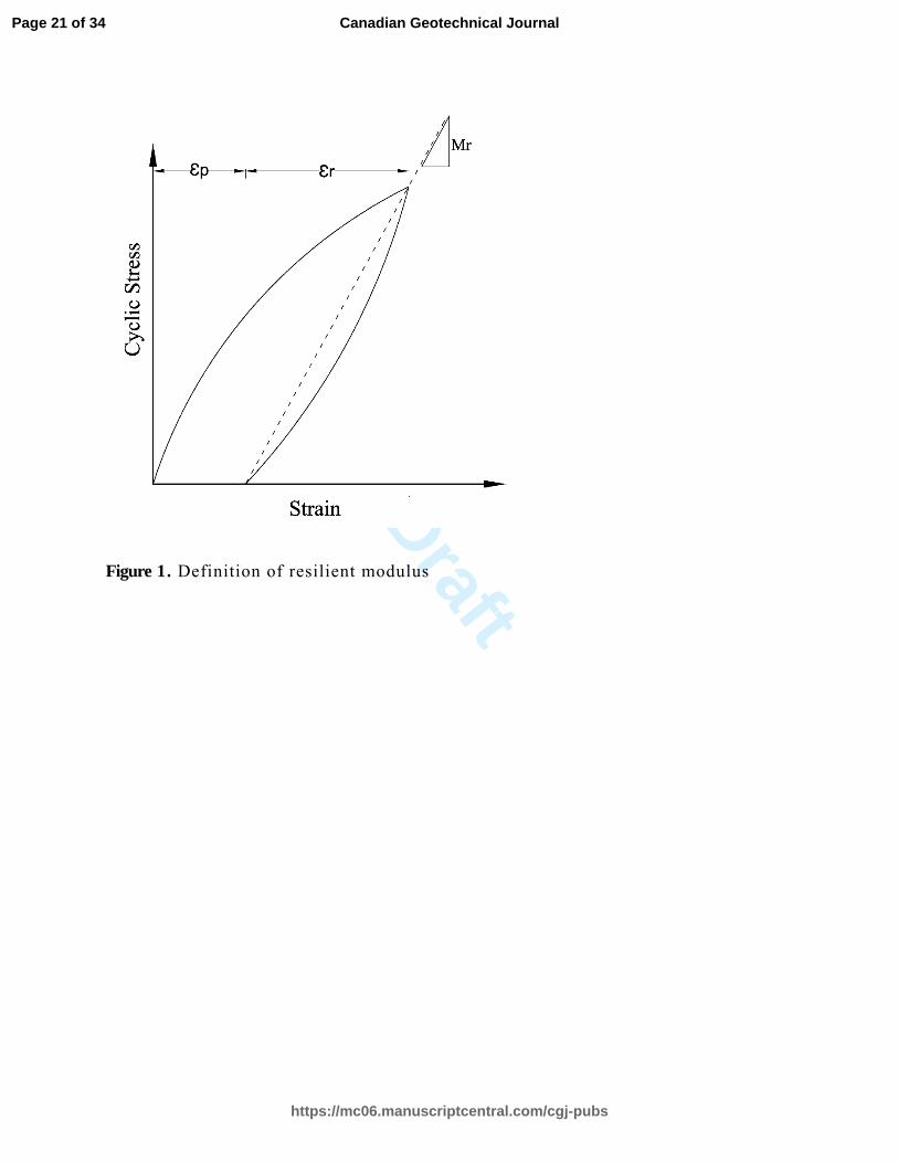
with an increase in deviatoric stress. The value of Mr is defined as the ratio of the cyclic axial 55
stress to the recoverable or resilient axial strain (NCHRP project 1-28A, 2004), as shown 56
schematically in Fig. 1 and expressed in Equation 1: 57
cyclic
r
r
Mσ
ε= (1) 58
Where: 59
cyclicσ : cyclic axial stress 60
:rε resilient axial strain 61
62
Figure. 1. Definition of resilient modulus 63
64
The Mr of a subgrade layer can be determined from laboratory testing following the AASHTO T-65
307 test protocol, which uses fifteen stress combinations: five deviatoric stress levels 13.8, 27.6, 66
41.4, 55.2 and 69 kPa (2, 4, 6, 8 and 10 psi) applied at three confining pressures 41.4, 57.6 and 67
Page 3 of 34
https://mc06.manuscriptcentral.com/cgj-pubs
Canadian Geotechnical Journal

Draft
Mousavi, Gabr, Borden
5
13.8 kPa (6, 4 and 2 psi). Different forms of constitutive models can be found in the literature 68
that allow for computing the Mr value as a function of one, two or three stress parameters such as 69
confining pressure, deviatoric stress, bulk stress and octahedral shear stress (e.g. Dunlap 1963; 70
Seed et al. 1967; Witczak and Uzan 1988; Pezo 1993; NCHRP project 1-28A 2004). The recent 71
universal constitutive model proposed in NCHRP 1-28A (MEPDG) is presented in Equation 2: 72
32
1. .( ) .( 1)kk oct
rM k PaPa Pa
τθ= + (2) 73
Where: 74
:rM resilient modulus 75
:aP atmospheric pressure 76
1 2 3, , :σ σ σ principal stresses 77
1 32 :θ σ σ= + bulk stress 78
1 3
2( ) :
3octτ σ σ= − octahedral shear stress 79
:ik regression constants; i:1, 2, and 3 80
81
Despite the good accuracy of the use of laboratory testing to determine Mr. values, the 82
requirement of using an expensive and sophisticated device to perform the Mr test is considered 83
as a disadvantage. Several studies have been undertaken to overcome this issue by estimating Mr 84
through the development of empirical correlations with the physical properties of soil (e.g. 85
Carmichael et al. 1985; Elliott et al. 1988; Drumm et al. 1990; Farrar and Turner 1991; Hudson 86
et al. 1994). These empirical correlations eliminate the expense of resilient modulus laboratory 87
testing, but they are generally not capable of capturing the stress dependency of the Mr, or 88
simulate various stress conditions encountered in the field. Many studies have been performed 89
Page 4 of 34
https://mc06.manuscriptcentral.com/cgj-pubs
Canadian Geotechnical Journal
Draft
Mousavi, Gabr, Borden
6
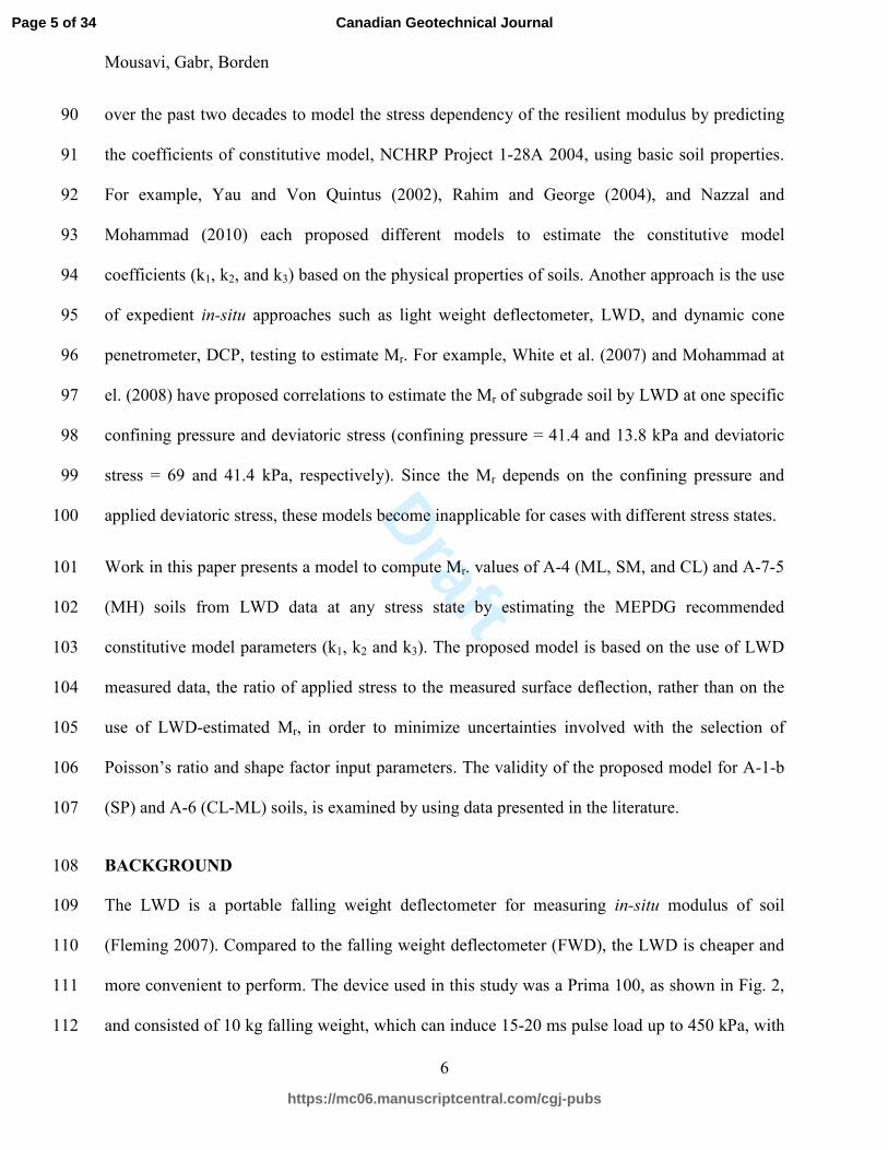
over the past two decades to model the stress dependency of the resilient modulus by predicting 90
the coefficients of constitutive model, NCHRP Project 1-28A 2004, using basic soil properties. 91
For example, Yau and Von Quintus (2002), Rahim and George (2004), and Nazzal and 92
Mohammad (2010) each proposed different models to estimate the constitutive model 93
coefficients (k1, k2, and k3) based on the physical properties of soils. Another approach is the use 94
of expedient in-situ approaches such as light weight deflectometer, LWD, and dynamic cone 95
penetrometer, DCP, testing to estimate Mr. For example, White et al. (2007) and Mohammad at 96
el. (2008) have proposed correlations to estimate the Mr of subgrade soil by LWD at one specific 97
confining pressure and deviatoric stress (confining pressure = 41.4 and 13.8 kPa and deviatoric 98
stress = 69 and 41.4 kPa, respectively). Since the Mr depends on the confining pressure and 99
applied deviatoric stress, these models become inapplicable for cases with different stress states. 100
Work in this paper presents a model to compute Mr. values of A-4 (ML, SM, and CL) and A-7-5 101
(MH) soils from LWD data at any stress state by estimating the MEPDG recommended 102
constitutive model parameters (k1, k2 and k3). The proposed model is based on the use of LWD 103
measured data, the ratio of applied stress to the measured surface deflection, rather than on the 104
use of LWD-estimated Mr, in order to minimize uncertainties involved with the selection of 105
Poisson’s ratio and shape factor input parameters. The validity of the proposed model for A-1-b 106
(SP) and A-6 (CL-ML) soils, is examined by using data presented in the literature. 107
BACKGROUND 108
The LWD is a portable falling weight deflectometer for measuring in-situ modulus of soil 109
(Fleming 2007). Compared to the falling weight deflectometer (FWD), the LWD is cheaper and 110
more convenient to perform. The device used in this study was a Prima 100, as shown in Fig. 2, 111
and consisted of 10 kg falling weight, which can induce 15-20 ms pulse load up to 450 kPa, with 112
Page 5 of 34
https://mc06.manuscriptcentral.com/cgj-pubs
Canadian Geotechnical Journal
Draft
Mousavi, Gabr, Borden
7
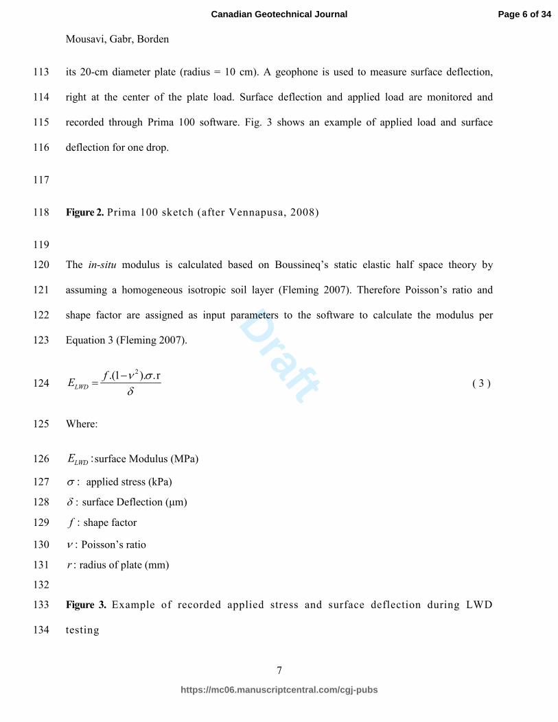
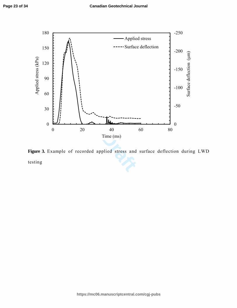
its 20-cm diameter plate (radius = 10 cm). A geophone is used to measure surface deflection, 113
right at the center of the plate load. Surface deflection and applied load are monitored and 114
recorded through Prima 100 software. Fig. 3 shows an example of applied load and surface 115
deflection for one drop. 116
117
Figure 2. Prima 100 sketch (after Vennapusa, 2008) 118
119
The in-situ modulus is calculated based on Boussineq’s static elastic half space theory by 120
assuming a homogeneous isotropic soil layer (Fleming 2007). Therefore Poisson’s ratio and 121
shape factor are assigned as input parameters to the software to calculate the modulus per 122
Equation 3 (Fleming 2007). 123
2.(1 ). .rLWD
fE
ν σ
δ
−= ( 3 ) 124
Where: 125
:LWDE surface Modulus (MPa) 126
:σ applied stress (kPa) 127
:δ surface Deflection (µm) 128
:f shape factor 129
:ν Poisson’s ratio 130
:r radius of plate (mm) 131
132
Figure 3. Example of recorded applied stress and surface deflection during LWD 133
testing 134
Page 6 of 34
https://mc06.manuscriptcentral.com/cgj-pubs
Canadian Geotechnical Journal
Draft
Mousavi, Gabr, Borden
8
As previously mentioned, there are few empirical correlations to approximate the Mr of subgrade 135
soil from LWD measurements. Although the main advantage of these models is that they can 136
capture actual moisture and density conditions of the soil layer, they are mostly limited to one 137
specific stress state. White et al. (2007) proposed the model presented in Equation 4 to predict Mr 138
of subgrade soil from ELWD with an assumed Poisson’s ratio of 0.35 and shape factor of 2
π and 2 139
for cohesive and cohesionless soils, respectively, at a confining pressure = 41.4 kPa (6 psi) and 140
deviatoric stress = 69 kPa (10 psi). 141
( 45.3)
1.24
LWDr
EM
+= 142
(4) 143
With ,r LWDM E in MPa 144
Mohammad et al (2008) presented the model in Equation 5 in order to estimate Mr from LWD 145
data by assuming a Poisson’s ratio of 0.4 and a shape factor of 2
π for cohesive soil and 2 for 146
cohesionless soils, at a confining pressure 13.8 kPa (2 psi) and deviatoric stress 41.4 kPa (6 psi). 147
These stress values were chosen to represent the stress state at the top of the subgrade layer 148
under standard single axle loading of 80 kN (18 kips) and tire pressure of 689 kPa (100 psi) with 149
a 50-mm asphalt wearing course, 100-mm asphalt binder course and 200-mm aggregate base 150
course (Mohammad et al. 2008; Rahim and George 2004; Asphalt Institute 1989). 151
0.1827.75r LWDM E= × 152
(5) 153
With ,r LWDM E in MPa 154
Page 7 of 34
https://mc06.manuscriptcentral.com/cgj-pubs
Canadian Geotechnical Journal

Draft
Mousavi, Gabr, Borden
9
EXPERIMENTAL PROGRAM 155
A series of laboratory and in-situ LWD tests were performed to evaluate subgrade soil modulus 156
properties of four 4.88-m (16-ft) wide by 15.2-m (50-ft) long test sections located in the 157
Piedmont area, North of Greensboro, North Carolina. In this case, LWD testing was conducted in 158
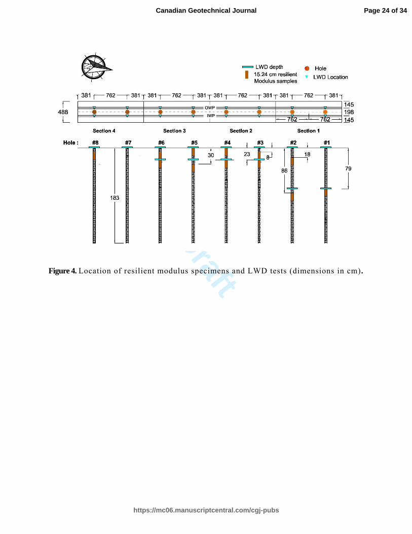
the field to monitor the variation of subgrade modulus across the test sections. As shown in Fig. 159
4, the LWD tests were carried out at four locations within each test section; those locations were 160
offset 1-m (3.3-ft) away from boreholes, from which Shelby tubes were obtained. In parallel, a 161
laboratory testing program including resilient modulus testing and physical properties 162
characterization was performed on undisturbed samples retrieved from within the LWD 163
influence zone, (a depth = 1.5~ 2 diameter of the LWD loading plate, as was specified by 164
Mooney and Miller 2007; Khosravifar et al. 2013; Senseney et al. 2016), as presented in Table 165
1, and indicated in Fig. 1. 166
167
Figure 4. Location of resilient modulus specimens and LWD tests (dimensions in cm). 168
169
MATERIALS 170
Basic index property tests, including grain size distribution, Atterberg limits, and specific gravity 171
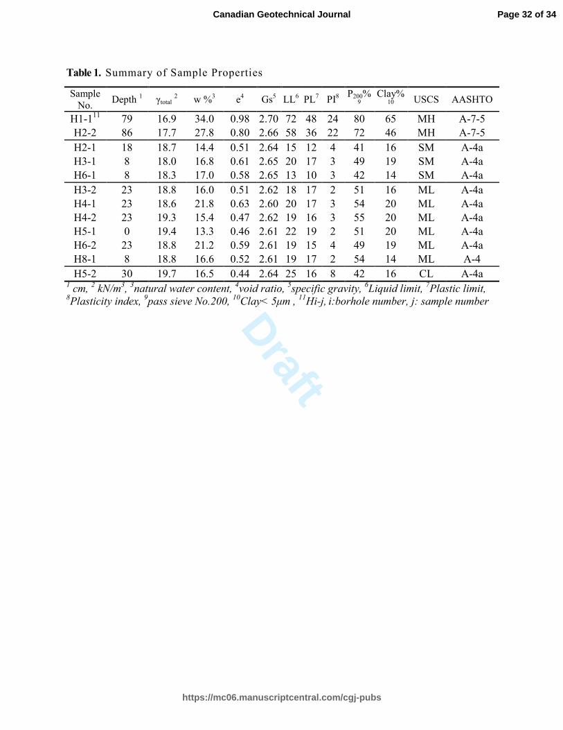
were conducted on the specimens after the Mr tests were completed. As shown in Table 1 and 172
Fig. 5, the site soils were classified as A-7-5 (MH), A4 and A4-a (SM, ML and CL, 173
respectively). The high plasticity specimens, A-7-5, were taken from the deeper depths, and 174
correspond to natural soil, while the low plasticity soils (A4 and A4-a) were located at shallower 175
depths and corresponded to compacted fill. 176
Page 8 of 34
https://mc06.manuscriptcentral.com/cgj-pubs
Canadian Geotechnical Journal
Draft
Mousavi, Gabr, Borden
10
177
Table 1. Summary of Sample Properties 178
179
Figure 5. Grain size distributions of resilient modulus samples 180
181
LWD MEASUREMENTS 182
Subgrade modulus values were measured at the test site by LWD (with 20 cm plate) following 183
the ASTM E2583-07. To do so, the plate is located horizontally on the surface, and first three 184
seating drops were considered to provide full contact between the plate load and the subgrade; 185
which followed by another three drops to obtain data for estimation of the surface modulus, 186
LWDE . The LWD
E values were calculated using Equation 3 and assuming a Poisson’s ratio of 187
0.35. A shape factor of 2
π was selected for the MH soil, and 2 for the ML, SM, and CL soil, 188
(Mooney and Miller 2007; White et al. 2007). Two LWD test stations were located about 1 m 189
apart on each side of the boreholes, from which samples for resilient modulus testing were 190
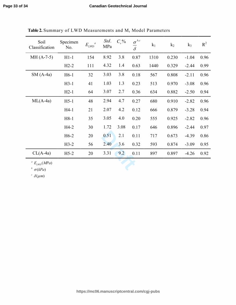
collected, as shown in Fig. 4. At each station, 3 ELWD were measured. The Standard deviation 191
and coefficient of variation of the six LWD measurements corresponding to the resilient modulus 192
laboratory specimen are presented in Table 2. The COVs are less than 5%. Hence for comparison 193
sake, the average of six field measured LWDE values was used to estimate the Mr from LWD. The 194
calculated Mr values were compared to the laboratory-measured Mr values for specimens 195
retrieved from the corresponding borehole within the LWD effective zone, as summarized in 196
Table 2. 197
As previously mentioned, the assumption of Poisson’s ratio and shape factor can lead to various 198
estimates of ELWD. In order to overcome the ambiguities with which values to use, the ratio of 199
Page 9 of 34
https://mc06.manuscriptcentral.com/cgj-pubs
Canadian Geotechnical Journal
Draft
Mousavi, Gabr, Borden
11
applied stress to surface deflection,σ
δ, from LWD direct measurements; which is representative 200
of soil layer elasticity, is directly used herein in the proposed model development, instead of 201
computing the ELWD by Equation 3. 202
The applied stress to surface deformation ratios from the LWD measurements are summarized in 203
Table 2 and are shown associated with the Specimen Number upon which the subsequent Mr 204
tests were performed. 205
LABORATORY TESTING: RESILIENT MODULUS 206
Resilient modulus tests were performed on undisturbed soil specimens following AASHTO T-207
307. Resilient modulus at each load combination was computed as the ratio of the cyclic axial 208
stress to average resilient axial strain for the last 5 of the 100 applied load cycles. Laboratory 209
results from each specimen were imported into MATLAB in order to evaluate fitting coefficients 210
for the MEPDG universal constitutive model, as presented in Equation 2. The calculated k1, k2, 211
and k3 values are provided in Table 2 along with the respective coefficient of determination (R2). 212
213
Table 2. Summary of LWD Measurements and Mr Model Parameters 214
215
EFFECT OF LWD INPUT PARAMETERS 216
Although input parameters such as Poisson’s ratio and shape factor can be approximated for 217
particular cases from values presented in literature, it is difficult to select appropriate values for 218
these input parameters for site specific conditions. Poisson ratio values between 0.2 to 0.5 are 219
recommended in the literature (Bishop 1977). Various shape factors are recommended for 220
Page 10 of 34
https://mc06.manuscriptcentral.com/cgj-pubs
Canadian Geotechnical Journal
Draft
Mousavi, Gabr, Borden
12
different scenarios. The shape factor can be varied between 2
π for a rigid loading plate, 1.33 and 221
2.67 for parabolic contact stress distribution in cohesive soils and granular soils, respectively, 222
and 2 for a uniform contact stress distribution (Terzaghi and Peck 1967; Mooney and Miller 223
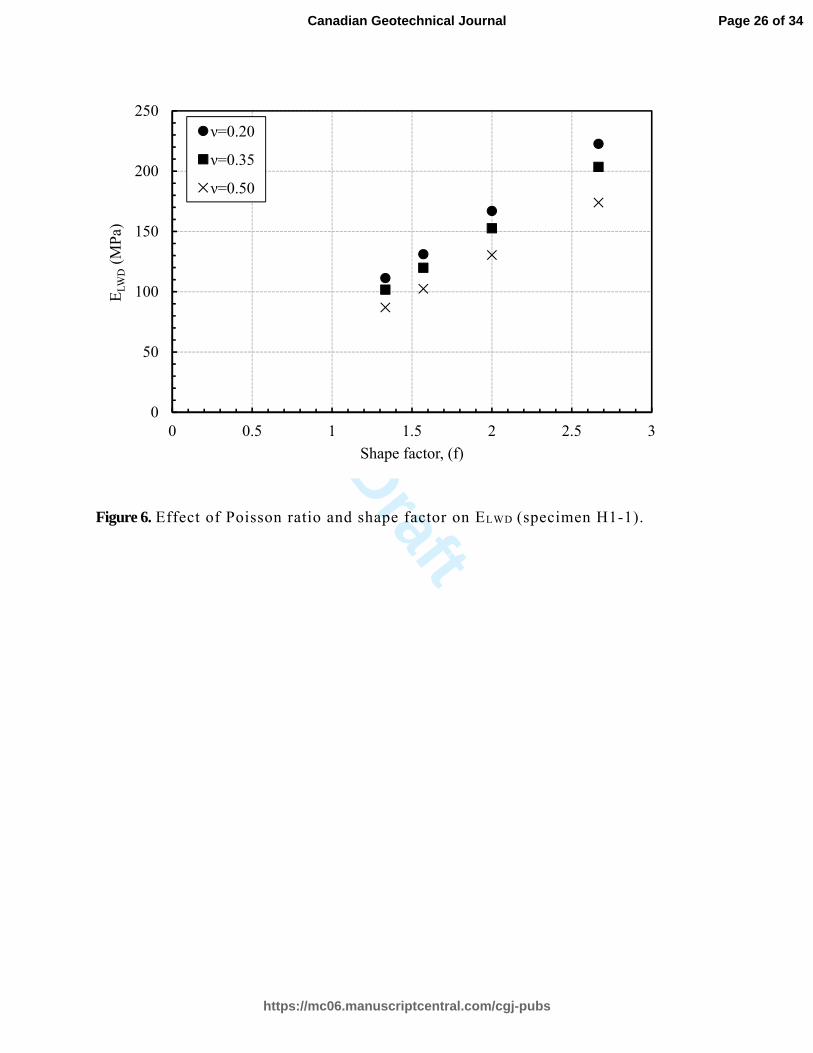
2007; Vennapusa and White 2007; Prima 100 software). The uncertainties associated with 224
selecting these parameters can induce significant variation in the value of calculated modulus, as 225
illustrated in Fig. 6. For the case shown, the computed LWDE for sample H1-1 can change from 226
110 up to 220 MPa by changing the shape factor from 1.33 to 2.67 at a given Poisson’s ratio of 227
0.2. In addition, it can be observed that the effect of Poisson’s ratio becomes more pronounced 228
with increasing shape factor, and can produce up to a 30% change in the computed elastic 229
modulus value. 230
231
Figure 6. Effect of Poisson ratio and shape factor on ELWD (specimen H1-1). 232
233
EXISTING MODELS 234
As previously mentioned, White et al. (2007) Mohammad et al (2008) proposed empirical 235
correlations to approximate the Mr of subgrade soil from LWD measurements at one specific 236
confining pressure and deviatoric stress. 237
The performance of these correlations in estimating the laboratory-measured Mr values from the 238
current study are both shown in Fig. 7. It can be seen that both correlations have generally 239
overpredicted the measured values; however the Mohammad et al. correlation underestimates the 240
Mr of the more highly plastic soils. 241
Page 11 of 34
https://mc06.manuscriptcentral.com/cgj-pubs
Canadian Geotechnical Journal

Draft
Mousavi, Gabr, Borden
13
242
Figure 7. Laboratory-measured Mr vs. that predicted from existing models 243
244
DEVELOPMENT OF LWD CORRELATION 245
As previously noted, the existing models for subgrade Mr determination from LWD data are 246
limited to a specific stress level. A change in pavement structure layer thickness, axial load, and 247
tire pressure can lead to changes in stresses within the layers. In order to overcome this 248
restriction and eliminate uncertainties associated with selecting appropriate Poison’s ratio and 249
shape factor values, the ratio of applied stress to surface deflection as measured during LWD 250
testing was used. The coefficients of the MEPDG model are functionally related to the elastic 251
modulus (k1), stiffness hardening (k2) and strain softening (k3) behavior of the soil (Yau and 252
Quintus, 2002). Accordingly, the proposed model was developed to correlate k1, k2, and k3 to the 253
ratio of σ
δ obtained from LWD measurements, with the advantage of having the ability to 254
estimate Mr. at other stress levels once these parameters are defined. The new model was 255
developed from regression analyses on the laboratory and field measurement data from the 256
cohesive (A-7-5) and cohesionless (A-4a) soils. 257
MEPDG COEFFICIENTS FROM LWD 258
Multilinear regression analyses was performed on three quarters of the data set to develop a 259
model to calculate resilient modulus indirectly at any stress level from LWD data through 260
estimating the MEPDG formula coefficients. The proposed correlation is presented in Equation 261
6, with the definition of constants presented in Table 3. Figs. 8(a-c) shows the calculated 262
coefficients, k1, k2, and k3, from curve fitting of the laboratory results versus the ratio of the 263
Page 12 of 34
https://mc06.manuscriptcentral.com/cgj-pubs
Canadian Geotechnical Journal
Draft
Mousavi, Gabr, Borden
14
measured applied stress to the surface deformation in the field. The proposed model predicts the 264
k1, k2 and k3 coefficients with a coefficient of determination ( R2) of 0.71, 0.82, and 0.55. 265
1 2 ( )ik C Cσ
δ= + 266
(6) 267
i :1,2,3 268
Table 3. Constant Coefficients of Developed Model 269
270
Figure 8. (a) Computed k1 vs. σ/δ, (b) Computed k2 vs. σ/ δ, and (c) Computed k3 vs. σ/δ. 271
Following AASHTO T-307, laboratory resilient modulus test is performed at 15 different stress 272
level, 5 deviatoric stress, 13.8, 27.6, 41.4, 55.2 and 69 kPa (2, 4, 6, 8 and 10 psi), at 3 confining 273
pressure, 41.4, 57.6 and 13.8 kPa (6, 4 and 2 psi); which provides 15 resilient modulus values 274
corresponding to each stress level. Hence for each specimen, 15 resilient moduli are measured at 275
different stress level. Fig. 9 shows the laboratory measured vs. predicted Mr, for ¾ of the 276
samples at 15 different stress levels. The analyses results, illustrated in Fig. 9, show that the 277
proposed model is able to compute the laboratory-measured Mr with a coefficient of 278
determination ( R2) of = 0.83. 279
Figure 9. Laboratory-measured Mr vs. that computed prediction 280
281
Model Validation 282
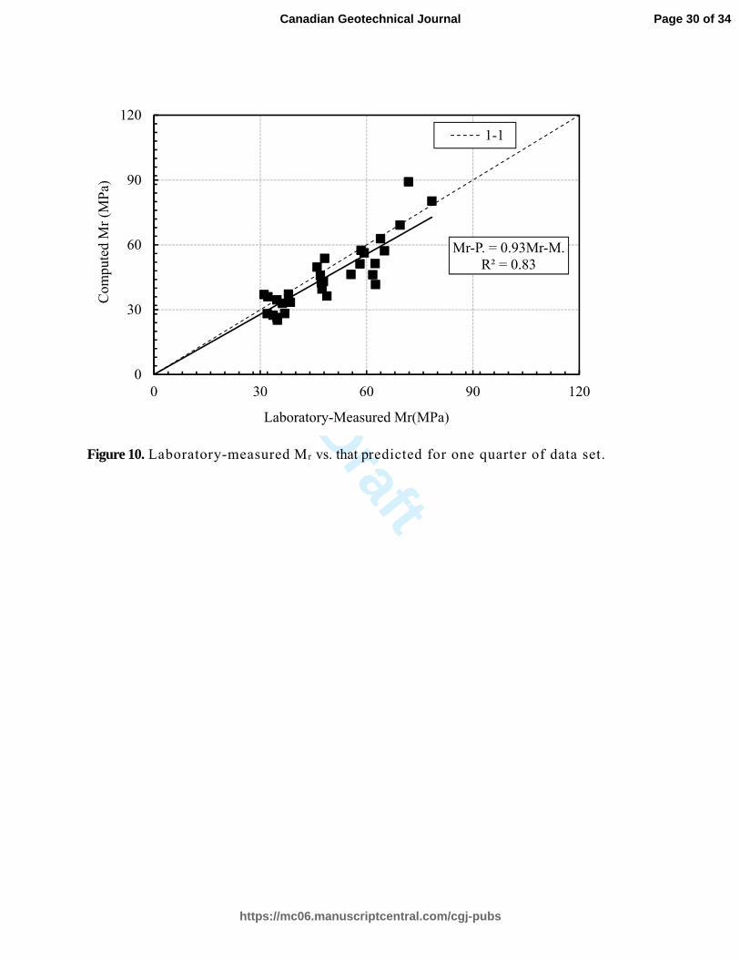
Fig. 10 shows laboratory-measured vs. model-computed resilient modulus values using the 283
remaining quarter of the data set which was not used in the initial statistical correlations, at 15 284
Page 13 of 34
https://mc06.manuscriptcentral.com/cgj-pubs
Canadian Geotechnical Journal

Draft
Mousavi, Gabr, Borden
15
different stress level. The best-fit line for the data plotted shows that the proposed model slightly 285
underestimates resilient modulus by 7% with a coefficient of determination of 0.83. The 286
performance of the proposed model was also evaluated by utilizing data available from two other 287
studies by White et al. (2007) and Mohammad et al. (2008). Data from White et al. (2007) 288
included LWD measurements as well as laboratory-measured Mr data at a confining pressure = 289
41.4 kPa (6 psi) and deviatoric stress = 69 kPa (10 psi), for A-6 (CL), sandy lean clay; and A-1-b 290
(SP) soil, poorly graded sand with silt and gravel. Mohammad et al. (2007) presented LWD and 291
Mr measurements at a confining pressure 13.8 kPa (2 psi) and deviatoric stress 41.4 kPa (6 psi), 292
for A-4(CL-ML) and A-6 (CL-ML) soils. In order to be able to utilize this data from the 293
literature, the ratio of σ
δvalues were back calculated using Equation 3. The parameters utilized 294
in the back-calculation were Poisson’s ratio of 0.35 and 0.4, for White et al. (2007) and 295
Mohammad et al. (2008), respectively, and shape factors of 2
π for cohesive soils and 2 for 296
cohesionless soils, as originally reported by the authors. As shown in Fig. 11, the proposed 297
model underestimates laboratory-measured Mr by 11% with a coefficient of determination of 298
0.96. 299
300
Figure 10. Laboratory-measured M r vs. that predicted for one quarter of data set. 301
302
Figure 11. Laboratory-measured Mr vs. that predicted using literature data. 303
304
Page 14 of 34
https://mc06.manuscriptcentral.com/cgj-pubs
Canadian Geotechnical Journal
Draft
Mousavi, Gabr, Borden
16
SUMMARY AND CONCLUSIONS 305
A model for estimating Mr on the basis of LWD data is presented in this paper. A performance 306
evaluation of existing models from the literature to assess Mr based on LWD data indicated a 307
limitation related to the ability of these model to predict Mr at only a single stress level. Using a 308
linear regression analyses approach, applied to laboratory measured Mr and field measured LWD 309
data, a new model is proposed to compute Mr at any desired stress state. The use of such a model 310
exclude uncertainties involved with the assumption of parameters needed for current LWD 311
modulus determination. In the proposed model, the ratio of applied stress to surface deformation 312
measured by LWD is used directly to compute MEPDG universal constitutive model coefficients 313
(k1, k2 and k3). Based on the results obtained in this study, the following conclusion can be 314
stated: 315
• The proposed model is capable of predicting Mr at various stress combinations with a 316
coefficient of determination of, (R2)0.83. Good agreement was obtained between the 317
LWD-predicted Mr and laboratory-measured data presented in other studies, with an 11% 318
average underprediction of Mr. values with R2 = 0.96. 319
• Examination of the ability of two existing models to predict Mr from in-situ LWD data, 320
showed a general trend toward overprediction, except for the higher plasticity soils tested 321
in this study. For this soil the Mohammad et al. correlation was seen to underestimate the 322
measured Mr. values. 323
• Input parameters needed to calculate elastic modulus by the LWD, such as Poisson’s ratio 324
and shape factor, can have a significant effect on the calculated ELWD. At a given 325
Poisson’s ratio, the ELWD can change by a factor of 2 depending on the shape factor 326
Page 15 of 34
https://mc06.manuscriptcentral.com/cgj-pubs
Canadian Geotechnical Journal

Draft
Mousavi, Gabr, Borden
17
selected. The effect of Poisson’s ratio was shown to increase with increasing shape 327
factor. 328
• The proposed model was demonstrated to predict the resilient modulus of A-1-b (SP), A-329
4 (ML, SM, CL), A-6 (CL-ML), and A-7-5 (MH) soil types using the measured ratio of 330
applied stress to surface deflection from a Prima 100 LWD device, employed in this 331
study. Further work will need to be performed to evaluate the applicability of the 332
proposed approach to other soil types as well. 333
Page 16 of 34
https://mc06.manuscriptcentral.com/cgj-pubs
Canadian Geotechnical Journal

Draft
Mousavi, Gabr, Borden
2
REFERENCES
AASHTO 2003. Standard method of test for determining the resilient modulus of soils and
aggregate materials. AASHTO T307-99, Washington, D.C.
Asphalt Institute, 1989, The Asphalt Handbook. Manual. Series No. 4 (MS-4), pp. 435-437.
ASTM D2216. 2010. Standard Test Methods for Laboratory Determination of Water (Moisture)
Content of Soil and Rock by Mass.
ASTM D422-63. 2007. Standard Test Method for Particle-Size Analysis of Soils.
ASTM D4318-10. Standard Test Methods for Liquid Limit, Plastic Limit, and Plasticity Index of
Soils.
ASTM D6913. 2009. Standard Test Methods for Particle-Size Distribution (Gradation) of Soils
Using Sieve Analysis.
ASTM D854. 2010. Standard Test Methods for Specific Gravity of Soil Solids by Water
Pycnometer.
ASTM E2583-07. 2011. Standard Test Method for Measuring Deflections with a Light Weight
Deflectometer (LWD).
Bishop, A. W., and Hight, D. W. 1977. “The value of Poisson’s ratio in saturated soils and rocks
stressed under undrained conditions”. Geotechnique 27, No. 3, pp 369-384.
Carmichael, R.F., III and Stuart, E. 1985. “Predicting Resilient Modulus: A Study to Determine
the Mechanical Properties of Subgrade Soils”. In Transportation Research Record: Journal of
the Transportation Research Board, No. 1043, Transportation Research Board, National
Research Council, Washington, D.C.,pp. 145–148.
Drumm, E.C., Boateng-Poku, Y., and Johnson Pierce, T. 1990. “Estimation of Subgrade
Resilient Modulus from Standard Tests”. Journal of Geotechnical Engineering, Vol. 116, No. 5,
pp. 774–789.
Dunlap, W.S. 1963. “A Report on a Mathematical Model Describing the Deformation
Characteristics of Granular Materials”. Technical Report 1, Project 2-8-62-27, Texas
Transportation Institute, Texas A&M University, College Station.
Elliot, R.P., Thorton, S.I., Foo, K.Y., Siew, K.W., and Woodbridge, R. 1988. “Resilient
Properties of Arkansas Subgrades”. Final Report, TRC-94, Arkansas Highway and
Transportation Research Center, University of Arkansas, Fayetteville.
Farrar, M.J., and Turner, J.P. 1991. “Resilient Modulus of Wyoming Subgrade Soils”. MPC
Report No. 91-1, Mountain Plains Consortium, Fargo, N.D.
Page 17 of 34
https://mc06.manuscriptcentral.com/cgj-pubs
Canadian Geotechnical Journal

Draft
Mousavi, Gabr, Borden
3
Fleming, P. R., Frost, M. W., and Lambert, J. P. 2007. “Review of Lightweight Deflectometer
for Routine in Situ Assessment of Pavement Material Stiffness”. In Transportation Research
Record: Journal of the Transportation Research Board, No. 2004, Transportation Research
Board of the National Academies, Washington, D.C., pp. 80–87.
Hudson, J.M., Drumm, E.C., and Madgett, M. 1994. “Design Handbook for the Estimation of
Resilient Response of Fine-Grained Subgrades”. Proceedings of the 4th International
Conference on the Bearing Capacity of Roads and Airfields, University of Minnesota,
Minneapolis, Vol. 2, pp. 917–931.
Khosravifar, S., Asefzadeh, A., and Schwartz, C. 2013. “Increase of Resilient Modulus of
Unsaturated Granular Materials During Drying After Compaction”. Geo-Congress 2013: pp.
434-443.
Li, D., and Selig, E. T. 1994. “Resilient Modulus for Fine-Grained Subgrade Soils”. Journal of
Geotechnical Engineering, Vol. 120, No. 6, pp 939-957.
Liang, R.Y., Rabab’ah, S., and Khasawneh, M. 2008. “Predicting moisture-dependent resilient
modulus of cohesive soils using soil suction concept”. Journal of Transportation Engineering,
134(1), pp.34-40.
Mohammad, L. N., Herath, A., Gudishala, R., Nazzal, M. D., Abu-Farsakh, M. Y., and Alshibli,
K. 2008. “Development of Models to Estimate the Subgrade and Subbase Layers’ Resilient
Modulus from In situ Devices Test Results for Construction Control”. Publication FHW-LA-
406. FHWA, U.S. Department of Transportation.
Mooney, M. A., and Miller, P. K. 2009. “Analysis of Lightweight Deflectometer Test Based on
In Situ Stress and Strain Response”. Journal of Geotechnical and Geoenvironmental
Engineering, Vol. 135, No. 2, pp 199-208.
Nazzal, M.D., and Mohammad, L.N. 2010. “Estimation of resilient modulus of subgrade soils for
design of pavement structures”. Journal of Materials in Civil Engineering, 22(7), pp.726-734.
NCHRP. 2003. “Harmonized test methods for laboratory determination of resilient modulus for
flexible pavement design”. Final Rep. NCHR Project No. 1-28 A, National Cooperative Highway
Research Program (NCHRP), Washington, D.C.
Pezo, R.F. 1993. “A General Method of Reporting Resilient Modulus Tests of Soils: A Pavement
Engineer’s Point of View”. Presented at the 72nd Annual Meeting of the Transportation
Research Board, Washington, D.C.
Rahim, A.M., and George, K.P. 2004. “Subgrade Soil Index Properties to Estimate Resilient
Modulus”. CD-ROM. Transportation Research Board of the National Academies, Washington,
D.C.
Page 18 of 34
https://mc06.manuscriptcentral.com/cgj-pubs
Canadian Geotechnical Journal
Draft
Mousavi, Gabr, Borden
4
Seed, H.B., Mitry, F.G., Monismith, C.L., and Chan, C.K. 1967. “NCHRP Report 35: Prediction
of Flexible Pavement Deflections from Laboratory Repeated-Load Tests”. Highway Research
Board, National Research Council, Washington, D.C.
Senseney, C.T., Grasmick, J., and Mooney, M.A. 2014. “Sensitivity of lightweight deflectometer
deflections to layer stiffness via finite element analysis”. Canadian Geotechnical Journal, 52(7),
pp. 961-970.
Terzaghi, K., and Peck, R. B. 1967. “Soil mechanics in engineering practice”. 2nd Ed., John
Wiley & Sons, Inc., New York.
Vennapusa, P.K., and White, D.J. 2009. “Comparison of light weight deflectometer
measurements for pavement foundation materials. Geotechnical Testing Journal, Vol. 32, No. 3,
pp. 1-13,
Witczak, M.W., and Uzan, J. 1988. “The Universal Airport Pavement Design System”. Report 1
of 4, Granular Material Characterization, University of Maryland, College Park.
White, D., Thompson, M., and Vennapusa, P. 2007. “Field Validation of Intelligent Compaction
Monitoring Technology for Unbound Materials”. Report No. MN/RC-2007-10.
Yau, A., and Von Quintus, H. 2002. “Study of laboratory resilient modulus test data and
response characteristics”, Rep. No. FHWA-RD-02-051, FHWA, U.S. Department of
Transportation, Washington, D.C.
Page 19 of 34
https://mc06.manuscriptcentral.com/cgj-pubs
Canadian Geotechnical Journal
Draft
Mousavi, Gabr, Borden
5
Figure captions
Figure 1. Definition of resilient modulus
Figure 2. Prima 100 sketch (after Vennapusa and White 2009)
Figure 3. Example of recorded applied stress and surface deflection during LWD
testing
Figure 4. Location of resilient modulus specimens and LWD tests (dimensions in cm).
Fig. 5. Grain size distributions of resilient modulus samples
Figure 6. Effect of Poisson ratio and shape factor on ELWD (specimen H1-1).
Figure 7. Laboratory-measured Mr vs. that predicted from existing models
Figure 8. (a) Computed k1 vs. σ/δ, (b) Computed k2 vs. σ/ δ, and (c) Computed k3 vs. σ/δ.
Figure 9. Laboratory-measured Mr vs. that computed prediction
Figure 10. Laboratory-measured Mr vs. that predicted for one quarter of data set.
Figure 11. Laboratory-measured Mr vs. that predicted using literature data.
Page 20 of 34
https://mc06.manuscriptcentral.com/cgj-pubs
Canadian Geotechnical Journal
Draft
Figure 1. Definition of resilient modulus
Page 21 of 34
https://mc06.manuscriptcentral.com/cgj-pubs
Canadian Geotechnical Journal

Draft
Figure 2. Prima 100 sketch (after Vennapusa and White 2009)
Page 22 of 34
https://mc06.manuscriptcentral.com/cgj-pubs
Canadian Geotechnical Journal
Draft
Figure 3. Example of recorded applied stress and surface deflection during LWD
testing
-250
-200
-150
-100
-50
00
30
60
90
120
150
180
0 20 40 60 80
Sur
face
def
lect
ion
(μm
)
App
lied
str
ess
(kP
a)
Time (ms)
Applied stress
Surface deflection
Page 23 of 34
https://mc06.manuscriptcentral.com/cgj-pubs
Canadian Geotechnical Journal
Draft
Figure 4. Location of resilient modulus specimens and LWD tests (dimensions in cm).
Page 24 of 34
https://mc06.manuscriptcentral.com/cgj-pubs
Canadian Geotechnical Journal

Draft
Figure 5. Grain size distributions of resilient modulus samples
0
10
20
30
40
50
60
70
80
90
100
0.0010.010.1110
Per
cen
t F
iner
, P%
Particle Diameter, D (mm)
MH (H1-1)
CL (H5-2)
ML (H4-2)
SM (H3-1)
Page 25 of 34
https://mc06.manuscriptcentral.com/cgj-pubs
Canadian Geotechnical Journal
Draft
Figure 6. Effect of Poisson ratio and shape factor on ELWD (specimen H1-1).
0
50
100
150
200
250
0 0.5 1 1.5 2 2.5 3
ELW
D(M
Pa)
Shape factor, (f)
ν=0.20
ν=0.35
ν=0.50
Page 26 of 34
https://mc06.manuscriptcentral.com/cgj-pubs
Canadian Geotechnical Journal

Draft
Figure 7. Laboratory-measured Mr vs. that predicted from existing models
0
30
60
90
120
150
180
0 30 60 90 120 150 180
Pre
dict
ed M
r (M
Pa)
Measured Mr (MPa)
White et al. (2007), A-4aWhite et al. (2007), A-7-5Mohammad et al. (2008), A-4aMohammad et al. (2008), A-7-51-1
Page 27 of 34
https://mc06.manuscriptcentral.com/cgj-pubs
Canadian Geotechnical Journal

Draft
Figure 8. (a) Computed k1 vs. σ/δ, (b) Computed k2 vs. σ/ δ, and (c) Computed k3 vs. σ/δ.
k3 = 2.80(σ/δ) - 3.8R² = 0.55
-5.0
-4.5
-4.0
-3.5
-3.0
-2.5
-2.0
-1.5
-1.0
-0.5
0.00.0 0.5 1.0
Com
pute
d k 3
σ/δ
(c)
k1 = 1040(σ/δ) + 480R² = 0.71
0
200
400
600
800
1000
1200
1400
1600
0.0 0.5 1.0
Com
pute
d k 1
σ/δ
(a)
k2 = -0.90(σ/δ) + 1R² = 0.82
0.0
0.2
0.4
0.6
0.8
1.0
1.2
0.0 0.5 1.0
Com
pute
d k 2
σ/δ
(b)
Page 28 of 34
https://mc06.manuscriptcentral.com/cgj-pubs
Canadian Geotechnical Journal

Draft
Figure 9. Laboratory-measured Mr vs. that computed prediction
R² = 0.83
0
40
80
120
160
0 40 80 120 160
Com
pute
d M
r (M
Pa)
Laboratory-Measured Mr(MPa)
A-4a
A-7-5
1-1
Page 29 of 34
https://mc06.manuscriptcentral.com/cgj-pubs
Canadian Geotechnical Journal
Draft
Figure 10. Laboratory-measured Mr vs. that predicted for one quarter of data set.
Mr-P. = 0.93Mr-M.R² = 0.83
0
30
60
90
120
0 30 60 90 120
Com
pute
d M
r (M
Pa)
Laboratory-Measured Mr(MPa)
1-1
Page 30 of 34
https://mc06.manuscriptcentral.com/cgj-pubs
Canadian Geotechnical Journal

Draft
Figure 11. Laboratory-measured Mr vs. that predicted using literature data.
Mr-Pr. = 0.89Mr-M.R² = 0.96
0
40
80
120
160
0 40 80 120 160
Pre
dict
ed M
r (M
Pa)
Laboratory-Measured Mr (MPa)
Mohammad et al.(2008)
White et al. (2007)
Page 31 of 34
https://mc06.manuscriptcentral.com/cgj-pubs
Canadian Geotechnical Journal
Draft
Table 1. Summary of Sample Properties
Sample
No. Depth
1 γtotal
2 w %
3 e
4 Gs
5 LL
6 PL
7 PI
8
P200%9
Clay%10
USCS AASHTO
H1-111
79 16.9 34.0 0.98 2.70 72 48 24 80 65 MH A-7-5
H2-2 86 17.7 27.8 0.80 2.66 58 36 22 72 46 MH A-7-5
H2-1 18 18.7 14.4 0.51 2.64 15 12 4 41 16 SM A-4a
H3-1 8 18.0 16.8 0.61 2.65 20 17 3 49 19 SM A-4a
H6-1 8 18.3 17.0 0.58 2.65 13 10 3 42 14 SM A-4a
H3-2 23 18.8 16.0 0.51 2.62 18 17 2 51 16 ML A-4a
H4-1 23 18.6 21.8 0.63 2.60 20 17 3 54 20 ML A-4a
H4-2 23 19.3 15.4 0.47 2.62 19 16 3 55 20 ML A-4a
H5-1 0 19.4 13.3 0.46 2.61 22 19 2 51 20 ML A-4a
H6-2 23 18.8 21.2 0.59 2.61 19 15 4 49 19 ML A-4a
H8-1 8 18.8 16.6 0.52 2.61 19 17 2 54 14 ML A-4
H5-2 30 19.7 16.5 0.44 2.64 25 16 8 42 16 CL A-4a 1 cm,
2 kN/m
3, 3natural water content,
4void ratio,
5specific gravity,
6Liquid limit,
7Plastic limit,
8Plasticity index,
9pass sieve No.200,
10Clay< 5µm ,
11Hi-j,
i:borhole number, j: sample number
Page 32 of 34
https://mc06.manuscriptcentral.com/cgj-pubs
Canadian Geotechnical Journal
Draft
Table 2. Summary of LWD Measurements and Mr Model Parameters
Soil
Classification
Specimen
No.
MPa
k1 k2 k3 R2
MH (A-7-5) H1-1 154 8.92 3.8 0.87 1310 0.230 -1.04 0.96
H2-2 111 4.32 1.4 0.63 1440 0.329 -2.44 0.99
SM (A-4a) H6-1 32 3.03 3.8 0.18 567 0.808 -2.11 0.96
H3-1 41 1.03 1.3 0.23 513 0.970 -3.08 0.96
H2-1 64 3.07 2.7 0.36 634 0.882 -2.50 0.94
ML(A-4a) H5-1 48 2.94 4.7 0.27 680 0.910 -2.82 0.96
H4-1 21 2.07 4.2 0.12 666 0.879 -3.28 0.94
H8-1 35 3.05 4.0 0.20 555 0.925 -2.82 0.96
H4-2 30 1.72 3.08 0.17 646 0.896 -2.44 0.97
H6-2 20 0.51 2.1 0.11 717 0.673 -4.39 0.86
H3-2 56 2.40 3.6 0.32 593 0.874 -3.09 0.95
CL(A-4a) H5-2 20 3.31 9.2 0.11 897 0.897 -4.26 0.92
a
LWDE.Std %
vC ,b c
σ
δ
( )
( )
( )
a
LWD
b
c
E MPa
kPa
m
σ
δ µ
Page 33 of 34
https://mc06.manuscriptcentral.com/cgj-pubs
Canadian Geotechnical Journal

Draft
Table 3. Constant Coefficients of Developed Model
C1 C2
k1 480 1040
k2 1.0 -0.9
k3 -3.7 2.8
Page 34 of 34
https://mc06.manuscriptcentral.com/cgj-pubs
Canadian Geotechnical Journal