
DRAFT February 24, 2014 - US Forest Service February 24, 2014 ... 4 Washington: a Synthesis of the...
403
Draft Manuscript has been technically reviewed and is currently in press Feb 24, 2014 1 DRAFT 1 February 24, 2014 2 The Ecology and Management of Moist Mixed-conifer Forests in Eastern Oregon and 3 Washington: a Synthesis of the Relevant Biophysical Science and Implications for Future Land 4 Management 5 6 Authors 7 Stine, Peter (Pacific Southwest Research Station, USDA Forest Service) 8 Hessburg, Paul (Pacific Northwest Research Station, USDA Forest Service) 9 Spies, Thomas (Pacific Northwest Research Station, USDA Forest Service) 10 Kramer, Marc (University of Florida) 11 Fettig, Christopher J. (Pacific Southwest Research Station, USDA Forest Service) 12 Hansen, Andy (Montana State University) 13 Lehmkuhl, John (Pacific Northwest Research Station, USDA Forest Service, retired) 14 O’Hara, Kevin (University of California Berkeley) 15 Polivka, Karl (Pacific Northwest Research Station, USDA Forest Service) 16 Singleton, Peter (Pacific Northwest Research Station, USDA Forest Service) 17 Charnley, Susan (Pacific Northwest Research Station, USDA Forest Service) 18 Merschel, Andrew (Oregon State University) 19 20
Transcript of DRAFT February 24, 2014 - US Forest Service February 24, 2014 ... 4 Washington: a Synthesis of the...

Draft Manuscript has been technically reviewed and is currently in press Feb 24, 2014
1
DRAFT 1
February 24, 2014 2
The Ecology and Management of Moist Mixed-conifer Forests in Eastern Oregon and 3
Washington: a Synthesis of the Relevant Biophysical Science and Implications for Future Land 4
Management 5
6
Authors 7
Stine, Peter (Pacific Southwest Research Station, USDA Forest Service) 8
Hessburg, Paul (Pacific Northwest Research Station, USDA Forest Service) 9
Spies, Thomas (Pacific Northwest Research Station, USDA Forest Service) 10
Kramer, Marc (University of Florida) 11
Fettig, Christopher J. (Pacific Southwest Research Station, USDA Forest Service) 12
Hansen, Andy (Montana State University) 13
Lehmkuhl, John (Pacific Northwest Research Station, USDA Forest Service, retired) 14
O’Hara, Kevin (University of California Berkeley) 15
Polivka, Karl (Pacific Northwest Research Station, USDA Forest Service) 16
Singleton, Peter (Pacific Northwest Research Station, USDA Forest Service) 17
Charnley, Susan (Pacific Northwest Research Station, USDA Forest Service) 18
Merschel, Andrew (Oregon State University) 19
20

Draft Manuscript has been technically reviewed and is currently in press Feb 24, 2014
2
Abstract 1
Stine, Peter; Hessburg, Paul; Spies, Thomas; Kramer, Marc; Fettig, Christopher J.; Hansen, 2
Andy; Lehmkuhl, John; O’Hara, Kevin; Polivka, Karl; Singleton, Peter; Charnley, Susan; 3
Merschel, Andrew. 2014. The ecology and management of moist mixed-conifer forests in eastern 4
Oregon and Washington: a synthesis of the relevant biophysical science and implications for 5
future land management. Gen. Tech. Rep. PNW-GTR-XXX. Portland, OR: U.S. Department of 6
Agriculture, Forest Service, Pacific Northwest Research Station. XX p. 7
8
Land managers in the Pacific Northwest have reported a need for updated scientific information 9
on the ecology and management of mixed-conifer forests east of the Cascade Range in Oregon 10
and Washington. Of particular concern are the moist mixed-conifer forests, which have become 11
drought-stressed and vulnerable to high-severity fire after decades of human disturbances and 12
climatic warming. This synthesis responds to this need. We present a compilation of existing 13
research across multiple natural resource issues, including disturbance regimes, the legacy 14
effects of past management actions, wildlife habitat, watershed health, restoration concepts from 15
a landscape perspective, and social and policy concerns. We provide considerations for 16
management, while also emphasizing the importance of local knowledge when applying this 17
information at the local and regional level. 18
19
Keywords: moist mixed-conifer forests, landscape restoration, land management, resilience, 20
stewardship 21
22

Draft Manuscript has been technically reviewed and is currently in press Feb 24, 2014
3
Contents 1
Executive Summary 2
Moist Mixed-conifer Forests 3
Key Management Considerations 4
Potential Applications 5
Section 1 – Introduction 6
a. Purpose and Scope of This Synthesis 7
b. Current Management Context and Restoration Mandate 8
c. Structure of the Report – Where to Find Sections of Interest 9
Section 2 – Definition of Moist Mixed-conifer and Regional Context 10
Section 3 – Ecological Principles of Restoration and Landscapes 11
a. The Concept of Resilience 12
b. Ecological Principles for Landscape Planning and Management 13
Section 4 – Scientific Foundations 14
a. Ecological Composition, Patterns, and Processes prior to Euro-American Settlement (~1850) 15
b. Human Impacts to Moist Mixed-conifer Systems: Influences of the Last ~ 100-150 Years 16
c. Current Socioeconomic Context 17
d. Summary of Key Scientific Findings and Concepts 18
Section 5 – Management Considerations 19
a. Key Concepts for Management 20
b. Stand Management – Silvicultural Tools and their Role in Landscape Management 21
Section 6 – Institutional Capacity and Social Agreement for Restoring Moist Mixed-22
Conifer Forests 23

Draft Manuscript has been technically reviewed and is currently in press Feb 24, 2014
4
a. Social Acceptability of Restoration Treatments among Members of the Public 1
b. Collaboration 2
c. Institutional Capacity 3
Section 7 – Conclusions 4
Literature Cited 5
Glossary 6
Appendices 7
A. List of Practical Considerations for Landscape Evaluation and Restoration Planning 8
B. Regional-scale Fire Regimes Group Classification for Oregon and Washington 9
C. Reconstructed Historical Vegetation Conditions within Sampled Areas of the Blue Mountains 10
Province 11
12

Draft Manuscript has been technically reviewed and is currently in press Feb 24, 2014
5
Executive Summary 1
Millions of hectares of western forests have been negatively affected by drought and insect and 2
disease outbreaks, and are overloaded with fuel, priming them for unusually severe and large 3
wildfires. In light of these trends, public support for forest restoration has grown. One priority of 4
the USDA Forest Service is to restore resiliency to forest and range ecosystems, enabling them to 5
cope with an uncertain future. Natural resource managers and policy makers are awash in 6
information from the growing body of science, with little time to sort through it, let alone 7
assimilate the many different sources and interpretations of the best available science. 8
9
Regional research and management executives requested a succinct review of the large body of 10
scientific information on eastside moist mixed-conifer (MMC) forests within the context of the 11
broader forest landscape in eastern Oregon and Washington. This focus was motivated by a lack 12
of up-to-date management guidelines, scientific synthesis, and consensus among stakeholders 13
about management direction in the diverse MMC type. 14
15
Understanding complex ecological and social processes and functions across landscapes requires 16
an integrated assessment that combines multiple scientific disciplines across spatial and temporal 17
scales. We therefore produced this science synthesis, which compiles existing research, makes 18
connections across disparate sources, and addresses multilayered natural resource issues. This is 19
provided to land managers to assist in updating existing management plans and on-the-ground 20
projects intended to promote resilience in MMC forests. We consider management flexibility at 21
the local scale critically important for contending with specific legacy effects of management 22

Draft Manuscript has been technically reviewed and is currently in press Feb 24, 2014
6
and the substantial ecological variation in MMC forest conditions, as well as for adapting 1
management to local social and policy concerns. 2
3
Our hope is that this synthesis serves as a reference that provides a condensed and integrated 4
understanding of the current state of knowledge regarding MMC forests, as well as an extensive 5
list of published sources where readers can find further information. But we also hope to enhance 6
cross-disciplinary communication and enrich dialogue among Forest Service researchers, 7
managers, and external stakeholders as we address common restoration concerns and 8
management challenges for MMC forests in eastern Oregon and Washington. 9
10
Key sections of this synthesis include: 11
A description of MMC forests and their context in the broader landscape of eastern 12
Oregon and Washington. 13
Key concepts of restoration and the landscape perspective. 14
A comprehensive summary of pre-European settlement conditions in MMC forests. 15
A description of the socioeconomic context in the region. 16
A summary of human impacts on MMC forests. 17
Broad management implications. 18
A practical list of management considerations for diagnosing restoration needs and 19
designing landscape approaches. 20
21
Moist Mixed-conifer Forests 22

Draft Manuscript has been technically reviewed and is currently in press Feb 24, 2014
7
Mixed-conifer forests are a major component of the dry-to-wet conifer forest complex that is 1
widely distributed across eastern Oregon and Washington. These forests are important for, 2
among other factors, carbon sequestration, watershed protection, wildlife habitat, and outdoor 3
recreation, and they provide economic opportunities through provisioning of a wide variety of 4
forest products. MMC forests cover a large area east of the crest of the Cascades in Oregon and 5
Washington where grand fir, white fir, and Douglas-fir are the dominant late-successional tree 6
species. MMC forests can be considered intermediate between drier conifer forests where pine 7
was historically dominant and fire was typically frequent and low in severity, and wetter or 8
cooler mixed-conifer forests where fire was less frequent and burned at higher severities. The 9
MMC forest type is in a central position along a complex moisture, composition, and disturbance 10
gradient of conifer forests in this region. This forest type is diverse and difficult to define, but 11
potential vegetation types and current conditions can be used to help identify places where stands 12
and landscapes need restoration. Historically, the forest landscape (from dry to wet) was a 13
mosaic driven by variation in climate, soils, topography, and low- to mixed- and occasional high-14
severity fire. 15
16
Decades of wildfire suppression and exclusion, domestic livestock grazing, and selective and 17
clearcut timber harvesting have interacted to alter the structure, composition, and disturbance 18
regimes of these forests. MMC forests have become denser, have lost large individuals of fire-19
resistant tree species, and, on many sites, have become dominated by dense patches of shade-20
tolerant tree species that are less resistant to fire and less resilient to drought. These vegetation 21
changes and management activities have shifted fire regimes toward less frequent, but larger and 22
more severe fires, which tend to simplify the landscape into fewer, larger, and less diverse 23

Draft Manuscript has been technically reviewed and is currently in press Feb 24, 2014
8
patches resulting in more homogenous conditions. Currently, many mixed-conifer forests are 1
denser, more uniform in structure, and contain more live and dead fuel than they did historically. 2
But the relative effects of human-caused changes, like fire suppression and timber harvesting, on 3
these forests differ widely across the region. Thus, it is important to develop local, first-hand 4
knowledge of the historical and contemporary disturbance regimes of these forests. 5
6
Key Management Considerations 7
As we reviewed the scientific literature, our primary objective was to synthesize the large body 8
of information into succinct findings that are supported by credible research and relevant to 9
practitioners and others interested in management of MMC forests. Some of our findings 10
include: 11
12
Historical range of variation (HRV) is useful as a guide but not as a target. Returning to it is 13
no longer feasible or practical in some places because of changing climate, land use, and altered 14
forest structure and composition. The contemporary concept of restoration goes beyond the oft-15
stated goal of reestablishing ranges of resource conditions that existed at some time in the past 16
(e.g., prior to Euro-American settlement). Our ecological process-oriented approach supports 17
restoration of conditions that may have occurred in the past under certain circumstances. 18
However, the objective of ecological restoration is to create a resilient and sustainable forest 19
under current and future conditions. It must be forward looking. Managers have some capacity to 20
influence the future range of variability (FRV) to achieve desired future ecosystem conditions for 21
a landscape. 22
23

Draft Manuscript has been technically reviewed and is currently in press Feb 24, 2014
9
Disturbance regimes have been significantly altered after 150 years of Euro-American land 1
use. Wildfires (along with insects, pathogens, and weather) were the dominant disturbance 2
process shaping historical forest structure and composition. Low-, mixed-, and high-severity fires 3
occurred in MMC forests, varying in size and occurrence across ecoregions. Small and medium 4
fires were the most numerous, but large fires accounted for the majority of the area burned. 5
Forests today neither resemble nor function as they did 150 years ago. 6
7
Moist mixed-conifer forests are more vulnerable to large, high-severity fire and insect 8
outbreaks. Widespread anthropogenic changes have created more homogenized conditions in 9
this forest type, generally in the form of large, dense, and multilayered patches of fire-intolerant 10
tree species. These changes have substantially altered the resilience mechanisms associated with 11
MMC forests. 12
13
Patterns of vegetation structure and composition in an eastside forest landscape shaped by 14
intact disturbance regimes are diverse and differ over space and time. Resilience in these 15
forests depends on this ecological heterogeneity. Euro-American settlement and early 16
management practices put these landscapes on new and rapidly accelerating trajectories of 17
change in vegetation composition and structure. Despite the change and variability, topography, 18
soils, and elevation constrain these vegetation patterns and provide a template for understanding 19
and managing landscape patterns. For example, south-facing aspects and ridges tended to burn 20
more often and less severely than north-facing aspects and valleys. Landscape restoration 21
strategies can capitalize on these tendencies. 22
23

Draft Manuscript has been technically reviewed and is currently in press Feb 24, 2014
10
Several wildlife species of conservation concern require structural complexity typical of 1
mature and old forests, which are currently limited or at risk. With no action, maintaining 2
adequate area and spatial patterns of old-forest habitats will be a challenge with the anticipated 3
increases in severe fire and insect infestations expected in response to changed forest conditions 4
and climate change. Restoration at a landscape scale will have challenges in retaining existing 5
old-forest patches while transitioning to a more heterogeneous and resilient forest condition. 6
7
Community-based collaborative groups can facilitate restoration in eastside national 8
forests. One of the major constraints to increasing the pace and scale of restoration treatments on 9
lands administered by the National Forest System (NFS) in eastern Oregon has been the lack of 10
social agreement about how to achieve it. The Forest Service promotes collaboration as a means 11
for helping diverse stakeholder groups come together and find an agreeable path forward. The 12
creation of local groups and the Forest Service’s Collaborative Forest Landscape Restoration 13
Program both offer innovations and demonstrate opportunities to improve capacity for 14
restoration through collaborative processes. 15
16
Potential Applications 17
In the midst of complicated social and political forces, forest managers make decisions that 18
require the application of complex scientific concepts to project-specific conditions. Decisions 19
often must balance risks (e.g., elimination of fuels hazards vs. preservation of old-forest 20
conditions) while acknowledging and allowing for uncertainties. Decision makers also must 21
weigh tradeoffs associated with alternative courses of action to obtain multiple-use policy and 22

Draft Manuscript has been technically reviewed and is currently in press Feb 24, 2014
11
land management objectives. We acknowledge this difficult task and the concurrent need to have 1
and thoughtfully apply the best available scientific information. 2
3
It is not the role of the research community to direct management decisions. However, synthesis 4
of research, identification of core scientific findings, and discernment of management 5
implications in specific contexts are appropriate roles. Research also has a role of working 6
alongside managers to learn from successes and failures. We provide considerations for 7
management and emphasize that their application to local and regional landscapes requires the 8
skill and knowledge of practitioners to determine how best to apply them to a local situation with 9
its particular management history. Legacy effects do matter, and one size does not fit all. 10
11
In section 5.a, we synthesize principle findings gleaned from the body of scientific literature 12
(summarized in Section 4) as they pertain to management of MMC forests. These constitute the 13
“take-home” messages that are intended to assist land managers in the execution of their work. 14
15
The social agreement and institutional capacity for restoring MMC forests is every bit as 16
important as the scientific foundation for doing so. The ability to institute the kinds of changes 17
managers will consider is directly a function of the capacity of the larger community to form 18
working partnerships and a common vision. 19
20
Some of the potential changes in forest management evoked within this document represent a 21
departure from “business as usual.” Land managers will decide how to proceed, and this will 22
depend in large part on budget, policy, local circumstances, and ultimately the judgment of line 23

Draft Manuscript has been technically reviewed and is currently in press Feb 24, 2014
12
officers. However, there are some ideas and observations from past work, both research and 1
management, that suggest the need for some prudent adjustments in management approach. 2
3
4

Draft Manuscript has been technically reviewed and is currently in press Feb 24, 2014
13
Section 1 – Introduction 1
2
“There is and always will be uncertainty and unpredictability in managed ecosystems, both as humans 3
experience new situations and as these systems change because of management. 4
Surprises are inevitable. Active learning is the way in which this uncertainty is winnowed. Adaptive 5
management acknowledges that policies must satisfy social objectives but also must be continually 6
modified and be flexible for adaptation to these surprises. Adaptive management therefore views policies 7
as hypotheses—that is; most policies are really questions masquerading as answers. Since policies are 8
questions, then management actions become treatments in the experimental sense. The process of 9
adaptive management includes highlighting uncertainties, developing and evaluating hypotheses around 10
a set of desired system outcomes, and structuring actions to evaluate or ‘test’ these ideas.” 11
Lance Gunderson (2000), Ann. Rev. Ecol. Sys. 12
13
1.a Purpose and Scope of this Synthesis 14
Fire-prone mixed-conifer forests east of the crest of the Cascade Range in Oregon and 15
Washington (hereafter, “the east side”) provide clean water, recreation, wildlife habitat, and 16
many other important ecosystem goods and services. However, over the last century, many of 17
these forests have become denser and less resilient to disturbance as a result of human activity, 18
altered disturbance regimes, and climatic warming. In the last few decades, many of these forests 19
have also become further drought stressed and increasingly vulnerable to high-severity fire 20
(Westerling et al. 2006) and insect outbreaks as a result of climate change (Preisler et al. 2012) 21
(fig. 1). 22
23

Draft Manuscript has been technically reviewed and is currently in press Feb 24, 2014
14
In the Pacific Northwest, research and management executives from the USDA Forest Service 1
recently highlighted the need to update management guidance, scientific synthesis, and 2
consensus among stakeholders regarding these challenges. This synthesis responds to this need. 3
In particular, executives asked us to focus on eastside moist mixed-conifer (MMC) forests (see 4
definition in Section 2), within the context of the broader forest landscape on the east side. We 5
have written this synthesis for a diverse audience of forest planners, managers, and engaged 6
citizens. 7
8
For this effort, we convened a team of government and university scientists to review the 9
literature, synthesize knowledge and management options, and compile a bibliography. Team 10
members were selected based on their experience and expertise, spanning a range of disciplines 11
including aquatic ecology and fish biology, climate change, disturbance ecology, fire and forest 12
ecology, landscape ecology, silviculture, social science, and wildlife biology. 13
14
We focused the synthesis on the ecology of MMC forests but acknowledge that decision makers 15
must address major issues surrounding the needs and values of human communities, so these 16
decision processes are addressed as well. The forests of the east side represent complex 17
patchworks of temperature, moisture, productivity, climate, and disturbance regimes, and 18
associated forest types (fig. 2), and so we occasionally discuss forest types that adjoin the MMC 19
type to improve context. The synthesis specifically addresses: 20
Vegetation, landscape, and disturbance ecology. 21
Wildlife habitats and populations; and aquatic ecosystems and associated species. 22
Landscape approaches and perspectives. 23
Draft Manuscript has been technically reviewed and is currently in press Feb 24, 2014
15
Silvicultural approaches. 1
Climate change influences and climate futures. 2
3
Research findings summarized here can make a valuable contribution to restorative management, 4
but it will be up to managers and program leads to consider the unique ecological conditions of 5
each landscape and to determine how this information guides specific land management 6
decisions. To that end, findings here are intended to conceptually frame—not prescribe—land 7
management. Such guidance is available in the new Forest Service Planning Rule (36 CFR Part 8
219), an important new administrative rule of the Forest Service that applies current science to 9
planning and management. We consider management flexibility at the local site level critically 10
important for contending with specific legacy effects of management and the substantial 11
ecological variation in MMC forest conditions, as well as for adapting management to local 12
policy concerns. 13
14
In related dry mixed-conifer and ponderosa pine (Pinus ponderosa) forest types, research and 15
social license to begin restoration is relatively more advanced (e.g., see Franklin et al. 2013, Jain 16
et al. 2012), and managers are proceeding with restoration treatments (e.g., see Hessburg et al. 17
2013, OWNF 2012). However, we include the pine and dry mixed-conifer types in our 18
discussions because these dry and MMC types are entwined spatially and ecologically in eastern 19
Oregon and Washington. 20
21
1.b Current Management Context and Restoration Mandate 22
23

Draft Manuscript has been technically reviewed and is currently in press Feb 24, 2014
16
Federal and state forest managers are charged with maintaining and restoring diverse, resilient 1
(see Glossary), and productive forests in these fire-prone landscapes. Restoration can increase 2
the resilience of eastside MMC forests, and reduce the ecological costs of high-severity wildfire 3
and economic costs of fire suppression activities and post-fire rehabilitation, along with the 4
ecological and socioeconomic threats to adjoining state, private, and tribal lands. But achieving 5
these goals is challenging without sufficient investment. Twentieth-century harvesting of large 6
trees has reduced commercial operability in many eastside forests (e.g., see Rainville et al. 7
2008), and the value of remaining commercial products are often insufficient to cover the costs 8
of restoration. 9
10
Developing and implementing sound management strategies requires up-to-date knowledge of 11
biological and physical processes that regulate forest ecosystem structure and function, as well as 12
how humans have modified them, especially disturbance processes, which are a key to sculpting 13
habitat and structural patterns (e.g., see Spies 1998). In this context, a number of factors are 14
particularly relevant to eastside MMC forests: 15
The processes and patterns of eastside forests have been altered over the past 100 to 150 16
years (depending upon location) by the combined cumulative effects of mining, livestock 17
grazing, road and railroad construction, conversion of grasslands and shrublands to agriculture, 18
timber harvesting, fire suppression and exclusion, urban and rural development, invasions of 19
alien plant and animal species (including pathogens, insects, and aquatic organisms), expanding 20
infestations of native diseases and insects, and anthropogenic-induced climate change. 21
In many areas (e.g., those not burned in recent decades), today’s dry and MMC forests 22
are denser, have more small trees and fewer large fire-tolerant trees, and are dominated by shade-23

Draft Manuscript has been technically reviewed and is currently in press Feb 24, 2014
17
tolerant and fire-intolerant tree species. This has reduced fire and drought tolerance of these 1
forests. Large increases in surface and canopy fuel loads are widespread, resulting in greater risk 2
of large and often severe wildfires, especially during extreme fire weather conditions. 3
Furthermore, high stand densities increase competition for growing space among trees, thereby 4
reducing the amount of water and nutrients available to individual trees, and increasing their 5
susceptibility to some insect and disease disturbances. These changes threaten the long-term 6
sustainability of dry and MMC forests in general, and the long-term survival of remaining large 7
and very large trees, in particular, which persist in overcrowded conditions. 8
Climate change is already transforming forests in eastern Oregon and Washington 9
because it is linked to ongoing drought, and elevated levels of tree mortality attributed to insects, 10
diseases, and wildfire. This transformation is occurring at a brisk pace, and the window of 11
opportunity for effecting change in this trajectory is relatively short (likely a few decades). 12
Mandated conservation of threatened or endangered species, some of which have been 13
threatened by landscape alterations (first bullet above), has added ecological and regulatory 14
complexity to forest management. For example, in the eastern Cascades, restoration of dry and 15
MMC forests, fire regimes, and fuel patterns is often constrained by the need to minimize 16
disturbance in areas around active nest locations of the northern spotted owl (Strix occidentalis 17
caurina; NSO), in order to conserve its dense, late-successional and old-forest nesting, roosting, 18
and foraging habitats. 19
Currently, many landscapes of the east side have late-successional forest patterns that are 20
out of sync with past and current fire regimes, and are ecologically unsuited to providing large 21
contiguous areas of late-successional habitat over time. In addition, much of the structural 22
diversity in those stands is relatively short-lived because of the dominance of shade-tolerant tree 23

Draft Manuscript has been technically reviewed and is currently in press Feb 24, 2014
18
species. Conservation of habitat for old forest species including NSO, northern goshawk 1
(Accipiter gentilis), and pileated woodpecker (Dryocopus pileatus) needs to address the 2
sustainability and continuous recruitment of that habitat. The revised recovery plan for the NSO 3
(USFWS 2011) has called for an active management approach for sustaining and recruiting old 4
forest habitats in fire-prone forests of eastern Washington and Oregon. Similar considerations are 5
also an issue for species outside of the range of the NSO, particularly northern goshawks and 6
pileated woodpeckers. 7
Forest environments throughout the east side are ecologically and physiographically 8
variable: rates of change in forest conditions and effects of historical influences vary with forest 9
type, cultural geography, and physiographic region. Although broad-scale direction can have 10
value at times, one-size-fits-all solutions will generally not work. Instead, considerations of local 11
conditions, land use histories, and biophysical and landuse classifications can help address this 12
variability. 13
Managers report that maps of forest types across the east side are inconsistent in their 14
classifications of vegetation associations. This creates a supreme challenge for managing that 15
vegetation for myriad uses and habitats. Managers also lack adequately detailed characterizations 16
of how each forest type has been affected by natural, human, and climatic influences. 17
The relative merits of active versus passive management of forests to achieve ecological 18
and socioeconomic goals are subject to fierce debate, which is driven by wide-ranging and often 19
competing or conflicting societal values, and is not likely to subside. Many citizens have 20
expectations for sustainable delivery of ecosystem services from forests on public lands. 21
Delivery is confounded by uncertainties regarding the long- versus short-term effects of various 22
management practices on goods, services, and values. 23

Draft Manuscript has been technically reviewed and is currently in press Feb 24, 2014
19
1
In the western U.S., Forest Service priorities focus on restoring ecosystems, managing wildland 2
fires, and strengthening communities while providing jobs (Chief of the Forest Service address to 3
the Pinchot Institute, 2013). Restoration on public lands1 implies reenabling forests and 4
grasslands and their associated species to adequately cope with increased climate-related 5
stresses, and enhancing their recovery from climate-related disturbances, while continuing 6
delivery of forest-derived values, goods, and services to citizens. A central purpose of 7
restoration then is to re-establish the adaptive and resilient capacities of landscapes and 8
ecosystems in each unique physiographic region. A second related purpose is to restore the 9
adaptive capacity and social resilience of associated human communities, while restoring 10
ecological systems. The first purpose is served by restoring ecological patterns and processes that 11
are in synchrony with the biota, geology, and climate. The second is served by enabling human 12
communities to derive benefit from forest goods and services while conducting restoration and 13
maintenance activities. 14
15
The concept of restoration includes but is larger than the goal of reestablishing the historical 16
range of variability (HRV). A process-oriented approach supports restoring ranges of conditions 17
that have occurred in the past (e.g., eradicating invasive species and reconnecting fragmented 18
habitat of threatened or endangered species), in environments where the future climate will 19
strongly resemble the recent climate, and where the results are socially understood and 20
acceptable. Where the future climate is not expected to resemble the recent climate, the objective 21
of ecological restoration would be to create resilient forests and rangelands that are adapted to a 22
future climate. This idea is captured in the related notion of future range of variability, or FRV, 23

Draft Manuscript has been technically reviewed and is currently in press Feb 24, 2014
20
as coined by several authors (Binkley and Duncan 2010, Hessburg et al. 2013, Keane et al. 2009, 1
Moritz et al. 2011, Weins et al. 2012). In addition to being forward-looking, contemporary 2
concepts of ecological restoration may emphasize social context and the connectivity and 3
interactions among people, societies, and the biophysical elements of ecosystems. For some 4
landscapes, it will simply be impossible and inadvisable to return them to prior conditions 5
(Harris et al. 2006), while for others, it may be well advised. 6
7
To effectively implement restoration goals across eastside mixed-conifer forests, managers can 8
consider applying already completed assessments of conditions across the eastside landscape 9
(e.g., the Interior Columbia Basin Ecosystem Management Project and Eastside Forest 10
Ecosystem Health assessments), perhaps expanding on them, and then prioritizing the location 11
and nature of treatments that would be most beneficial to ecosystems and to people. This will 12
involve both regional and local landscape assessment. 13
14
In some places, there may be a need to increase the pace and scale of restoration to address a 15
variety of immediate threats—including fire, climate change, bark beetle infestations, and 16
others—for the health of public forest ecosystems, watersheds, and natural resource-dependent 17
communities. However, for these efforts to be sustainable, both ecological and socioeconomic 18
vantage points would be best considered in the context of regional and local landscape patterns 19
and processes, because in the long run, the natural system must support the social system. 20
21
1.c Structure of the Report – Where to Find Sections of Interest 22
23

Draft Manuscript has been technically reviewed and is currently in press Feb 24, 2014
21
Overview of contents—The report progresses from a review of the relevant science to a 1
presentation of management considerations. 2
3
Section 2 discusses how MMC types fit within a regional coniferous mosaic. In this section, the 4
reader will understand our definition of MMC forests, what forest types are typically included 5
within this classification, and generally where they are located. 6
7
Section 3 presents ecological concepts that are foundational to landscape restoration. 8
9
Section 4 explains and summarizes the detailed scientific information that constitutes our 10
synthesis. We provide a large number of citations to guide the reader through the scientific 11
literature. Major findings are also summarized in Section 4.d. Appendix C is provided to 12
complement Sections 4 and 5. 13
14
Section 5 is the core of this report, where the reader will find management concepts gleaned 15
from the scientific literature. We also provide a list of considerations that can help guide a 16
landscape evaluation process. This list arises from recent experiences of eastside land managers 17
who have adopted a landscape perspective and are conducting landscape evaluations. 18
Silvicultural options and innovations are discussed as they relate to landscape prescriptions and 19
their component stand-level prescriptions. We also present ideas about adjustments that may help 20
increase institutional capacity to implement the ideas contained in this report. We close this 21
section with an overview of the socioeconomic conditions that underlie most land management 22
decisions. 23

Draft Manuscript has been technically reviewed and is currently in press Feb 24, 2014
22
1
Section 6 provides a brief discussion of the important institutional considerations that influence 2
how these concepts might be implemented. This section also presents a summary discussion on 3
the socioeconomic issues that are clearly in the foreground of any management strategy that 4
seeks to restore the land and resources. 5
6
Section 7 provides brief conclusions and summary thoughts about how our findings may be 7
incorporated into land management and project-level plans. 8

Draft Manuscript has been technically reviewed and is currently in press Feb 24, 2014
23
Section 2 – Definition of Moist Mixed-conifer Forests and the Regional Context 1
Moist mixed-conifer (MMC) forests are diverse and cover a large area east of the crest of the 2
Cascades in Oregon and Washington where grand fir (Abies grandis), white fir (Abies concolor), 3
and Douglas-fir (Pseudotsuga menziesii) are the potential late-successional (climax) tree species 4
(fig. 3). These forests grow in environments that are subsets of the white fir–grand fir, and 5
Douglas-fir “series,” broad potential vegetation types used by Forest Service managers (Powell 6
et al. 2007, Simpson 2007) to characterize the land’s general ecological and vegetative 7
capability. 8
9
Depending upon the environment and local site climate, patches of MMC forest typically occur 10
where the current vegetation (not necessarily the same as potential natural vegetation or the 11
vegetation that would develop under historical fire regimes) is a mixture of shade-intolerant 12
ponderosa pine (Pinus ponderosa) or western larch (Larix occidentalis), and shade-tolerant 13
Douglas-fir, white or grand fir, and occasionally Engelmann spruce (Picea engelmannii), as in 14
the moist grand fir zone of the Blue Mountains (Powell 2007). In areas of complex, dissected 15
topography, the MMC forest intermingles with ponderosa pine and dry mixed-conifer types and 16
wetter or cooler conifer types (fig. 4; Powell et al. 2007, Simpson 2007). Other conifers 17
occasionally associated with MMC forest include lodgepole pine (Pinus contorta), western white 18
pine (Pinus monticola), sugar pine (Pinus lambertiana), Shasta red fir (Abies magnifica), Pacific 19
silver fir (Abies amabilis), and western hemlock (Tsuga heterophylla). Dry ponderosa pine and 20
dry mixed-conifer conditions tend to occupy lower montane settings, ridgetops, and southern 21
exposures, while MMC conditions typically occur in mid-to upper montane settings; on northerly 22
and sometimes southerly aspects, especially in the upper elevations; in valley bottoms; and in 23

Draft Manuscript has been technically reviewed and is currently in press Feb 24, 2014
24
lower headwall positions. 1
2
The focus of this report is not so much about forest of a particular moisture class, but mixed-3
conifer forests where fire exclusion has altered forest composition, structure, and function from 4
their historical range of variability. Wetter mixed-conifer forests, with longer fire return 5
intervals, may also have restoration needs, but these typically are not associated with changed 6
fire regimes and thus are not focus of this report. The historical vegetation of MMC forest was 7
controlled by frequent to moderately frequent fires (<20-50 years) that burned with mixed 8
severity, containing both low- and high-severity patches. In most parts of the MMC forest, this 9
fire frequency has been suspended, and disturbance regimes have been altered through a 10
combination of historical drivers including grazing, loss of Native American fire ignitions, and 11
active fire suppression. Consequently, the current MMC forest vegetation today contains a 12
significantly greater component of shade-tolerant tree species (e.g., white or grand fir or 13
understory Douglas-fir) than occurred in the historical vegetation. Under historical or more fire- 14
and drought-resilient states these shade-tolerant species would have been less common in the 15
understory in many areas, and large fire-resilient ponderosa pine, Douglas-fir, and western larch 16
would have dominated the canopy layer. See Appendix C for additional information about the 17
variety of historical forest conditions that occurred in the Blue Mountains forest province early in 18
the 20th
century. Data are adapted from the Interior Columbia Basin Assessment (Hessburg et al. 19
1999b, 2000a). 20
21
Dry mixed-conifer and ponderosa pine sites (ponderosa pine series or drier grand-fir/white, or 22
Douglas-fir subseries) typically experienced frequent fire return intervals (10-25 years), and 23

Draft Manuscript has been technically reviewed and is currently in press Feb 24, 2014
25
exhibited a relatively open forest structure. Wetter and cooler mixed-conifer sites experienced 1
longer fire return intervals (>50 years), and greater frequency of higher severity fire, and would 2
have had a component of older shade-tolerant trees in the overstory, with dense areas of multi-3
storied forest. Because few detailed fire history studies exist for the mixed-conifer forest in 4
general, we use potential vegetation types (PVTs, see discussion below) as a surrogate for the 5
fire regime and the degree to which mixed-conifer forests are departed in terms of composition 6
and structure. These potential natural vegetation types, which include both series and 7
approximations of subseries (e.g., dry, dry-moist, moist, and moist to wet variants of grand, 8
white, and Douglas-fir series) can be a starting place for identifying the environments and 9
locations of MMC forest (table 1). The PVTs used by managers (e.g., series, subseries, and plant 10
associations) are often the best available source of local information, but are only an approximate 11
surrogate for the fire regime of a site or local landscape. Figure 5 illustrates the continuum of 12
forest types found along an elevational gradient on the eastside of the Cascades and the 13
relationship of forest type to general fire regimes. 14
15
Variation in slope, topographic position and landscape context can create a high degree of 16
variation in fire regimes within the same PVT. For example, for a given PVT, areas with steep or 17
concave slopes often experience more high-severity fire than gentler and more convex slopes. 18
Likewise, MMC PVT patches embedded within large dry forest patches or adjacent to grass or 19
shrub patches may experience a higher fire frequency than they would if they were embedded in 20
MMC forest. Context matters, and is critical to interpreting the native fire regime. Final 21
determination of MMC forest for restoration purposes should be based on landscape context, 22
local environment, and disturbance history. Figure 6 provides a conceptual model of the complex 23

Draft Manuscript has been technically reviewed and is currently in press Feb 24, 2014
26
ecological setting in which we find MMC forests. There are many biological and physical 1
conditions that will influence what kind of vegetation is found at a site. 2
3
The MMC type is widely distributed across the east side (fig. 7) occupying particular 4
environments and elevations along the east slope of the Cascade Range and large patches within 5
the northern and central portions of the Blue Mountains. It often is sandwiched between the drier 6
mixed-conifer and pine types and cooler and wetter mixed-conifer types. Figure 7 is intended to 7
give a general depiction of the distribution of MMC forest. No standard, peer-reviewed maps of 8
dry, moist, or wet PVTs exist for the entire region. See Section 4.a for more details on source of 9
regional information and details on vegetation in general. 10
11
12
13
14

Draft Manuscript has been technically reviewed and is currently in press Feb 24, 2014
27
Section 3 – Ecological Principles of Restoration and Landscapes 1
Restoration of ecological processes and patterns requires a multi-scale spatial and temporal 2
perspective. Historically, the forests in eastern Oregon and Washington were diverse and 3
complex in their species composition and structure (e.g., tree sizes, ages, density, layering, 4
clumpiness). These patterns influenced the frequency, severity, and spatial extent of native 5
insect, disease, wildfire, and abiotic disturbance processes such that signature “disturbance 6
regimes” were apparent. However, a century or more of management has significantly altered 7
patterns of structure and composition, and as a direct consequence, the associated disturbance 8
regimes are highly altered as well. Figure 8 illustrates the large disparity in historic vs. current 9
species composition and structure of forests in eastern Oregon and Washington. 10
11
MMC forests were and continue to be hierarchically-structured systems with complex 12
interactions between spatial scales. Part of what concerns us today is uncertainty driven by these 13
cross-scale disturbance interactions. For example, very large wildfires, insect outbreaks, and 14
changes in winter snowpack and hydrology occurring at a regional scale threaten to alter meso-15
scale patterns and disturbance processes of local landscapes. Simply working at meso-scale 16
(local landscapes, e.g., watersheds and subwatersheds) does not address these concerns. The 17
answer lies in a regional- or ecoregional-scale solution. 18
19
At a meso-scale, patterns of forest structure and composition emerge, which are primarily 20
maintained by interactions among environments, topography, weather, soils, geomorphology, 21
and disturbances. But other broader and finer-scale patterns also exist, and these are also 22

Draft Manuscript has been technically reviewed and is currently in press Feb 24, 2014
28
influential to maintaining and changing meso-scale vegetation patterns over space and through 1
time. 2
3
Forest ecosystem responses to disturbances or weather changes can sometimes be non-linear, or 4
involve complex feedback loops or time lags, particularly when we allow for longer observation 5
periods. Thus, some interactions are relatively more unpredictable and may not manifest in any 6
sort of change in the short term, until some kind of threshold is reached (Malamud et al 1998, 7
Moritz et al. 2013, Peterson 2002). The challenge for scientists and managers seeking to restore 8
landscape resilience is to develop a better understanding of ecological complexity that can more 9
readily be translated into practical strategies for restoration. 10
11
Our review of recent theory, observation, and understanding in the field of landscape ecology 12
shows it is critical to consider long-term spatial and temporal phenomena prior to drawing 13
conclusions or developing simplified decision rules based solely on temporally short or narrow 14
geographic observation windows. 15
16
3.a The Concept of Resilience 17
The resilience of current and future forest ecosystems is a major concern of land managers today. 18
The concept of resilience promises a robust alternative to management goals based on static 19
conditions or simple applications of historical range of variability (HRV). However, resilience is 20
not an easily defined concept in a practical sense (Gunderson 2000). Furthermore, operational 21
metrics of resilience have received little attention to date (Carpenter et al. 2001). To become 22
more operational, resilience must be defined in terms of specific system attributes and in relation 23

Draft Manuscript has been technically reviewed and is currently in press Feb 24, 2014
29
to specific disturbances or perturbations. It is important to understand that resilience is a relative 1
term and is constrained by space and especially time. Eventually change will be significant 2
enough that a previously resilient system will reset itself into a new state. Thus, some bounding 3
of space and time is necessary to define resilient states. 4
5
Folke (2006) and Gunderson (2000) have identified three conceptual domains of resilience: (1) 6
engineering resilience, which focuses on recovery or return time to a stable equilibrium (e.g., 7
return to particular forest structure or composition); (2) ecological resilience, which focuses on 8
maintaining function and persistence with multiple equilibria (e.g., HRV); and (3) socio-9
ecological resilience which focuses on reorganization, adaptive capacity and multi-scale 10
interactions among the many community members, stakeholders, and responsible government 11
organizations which have an interest in the outcome of land management. Although we focus 12
mainly on ecological resilience in this report, we acknowledge that the ecological system is 13
imbedded in a socio-economic system that interacts with the ecological systems. 14
15
The degree of alteration of an ecosystem and its dynamics (patterns of change over time and 16
space) must be understood before we can consider if and how the system can be restored (fig. 9). 17
18
Westman (1978) suggested five characteristics that depict the potential resilience of a system, 19
which have merit. 20
Inertia: The resistance of a system to disturbance. 21
Elasticity: The speed with which a system returns after disturbance. 22

Draft Manuscript has been technically reviewed and is currently in press Feb 24, 2014
30
Amplitude: A measure of how far a system can be moved from a previous state and still 1
return. 2
Hysteresis: The lagging of an effect behind its cause, such as delayed response of the 3
system to a disturbance. 4
Malleability: The difference between the pre- and post- disturbance conditions. The 5
greater or lesser the malleability, the lesser or greater the system’s resilience. 6
7
These technical terms from systems analysis illustrate the complexity of system responses to 8
change and the challenge of restoring dynamic systems. The characteristics of resilience 9
described here are not all measured with equal ease; some may simply be immeasurable in a 10
short period because of a lack of historical data or reliable ecosystem models (Westman 1978). 11
Given these limitations on data availability and the overall understanding of ecosystem 12
interactions, we are reminded of a compelling need for employing an adaptive management 13
approach with both research and monitoring where we can track the results of management 14
efforts and follow disturbances and recovery efforts over a long term. This would give managers 15
the ability to inform subsequent management decisions with what was learned from previous 16
management decisions and thus make appropriate adjustments. It also suggests the value and 17
need for ecosystem models and tools that can include consideration and measurement of both 18
inertia and resilience. Early versions of these tools have given us a better understanding of the 19
complex dynamics of forest ecosystems and, in turn, how we can craft management strategies to 20
achieve desired outcomes. In short, management for ecosystem resilience necessitates iterative 21
steps to allow for adjustments at each juncture of trial and learning. 22
23

Draft Manuscript has been technically reviewed and is currently in press Feb 24, 2014
31
Resilience does not always result in desirable conditions on the land (Folke 2006). Degraded and 1
non-native vegetation can also be resilient in its own way; for example, landscapes dominated by 2
cheatgrass (Bromus tectorum), which is generally considered undesirable, can be resilient in the 3
face of restoration efforts by land managers. In this example, managers have experienced 4
significant difficulties attempting to restore sagebrush steppe ecosystems invaded by cheatgrass 5
(Chambers et al. 2009, D’Antonio et al. 2009). 6
7
Landscapes often have considerable inertia because of alterations of pattern and process after 8
more than a century of human activity. For example, Wallin et al. (1994) found that landscape 9
patterns generated by past forest management or disturbance can take decades or centuries to 10
restore (see also Heinselman 1973). Hysteresis (in a large dose) can operate in altered landscapes 11
to create undesirable resilience or a delay in desired response to management. For example, the 12
widespread accumulation of Douglas-fir (Pseudotsuga menziesii) and, to a lesser degree, grand 13
fir (Abies grandis) across many eastside landscapes now means that disturbance patches created 14
by management or wildfire are more likely to regenerate to Douglas-fir and grand fir than they 15
would have in the recent past. These relations can create significant challenges in executing 16
successful restoration due to the large scale of the effect. 17
18
3.b Ecological Principles for Landscape Planning and Management 19
Our perspective on the scientific principles underlying restoration of landscape resilience in 20
eastside landscapes is based on three central ideas: (1) the biophysical environment (i.e., 21
vegetation, climate, geology, and topography) and disturbances interact to control system 22
behavior at several key spatial and temporal scales; (2) Euro-American activities have altered 23

Draft Manuscript has been technically reviewed and is currently in press Feb 24, 2014
32
these ecological interactions and reduced landscape resilience; and (3) increasing resilience of 1
desired conditions requires management actions that restore processes and patterns at these key 2
scales. Without this broad geographic and ecosystem perspective that includes the past, present, 3
and future role of humans and the climate, it will be impossible to restore resilient forests across 4
a wide range of ecoregions and landscapes. Such a systems view should enable more effective 5
application of treatments to meet restoration or resilience goals. 6
7
We use the terms local and regional landscapes. We define local landscapes as variably-sized 8
areas, typically ranging in size from one to several subwatersheds (hydrologic unit code [HUC] 6 9
or 12-digit watersheds; Sieber et al. 1987, see also the National Hydrography Dataset at 10
http://nhd.usgs.gov/), or a watershed (HUC 5 or 10-digit watersheds), which reside in a single 11
ecological subregion (sensu Hessburg et al. 2000b), and exhibit characteristic patchworks of 12
successional stages and topography consistent with the climate, biota, physical processes, and 13
disturbance regimes of that subregion. Subwatersheds (i.e., HUC level 6) typically range in size 14
from about 4,000 to 16,000 hectares (10,000 to 40,000 acres), but larger and smaller 15
subwatersheds also occur. We define a regional landscape as the complete collection of all local 16
landscapes that comprise an ecological subregion. 17
18
We define (local or regional) landscape resilience as the capacity of the ecosystems to absorb 19
disturbance and climatic change while reorganizing and changing but essentially retaining the 20
same function, structure, identity, and feedbacks (adapted from Walker et al. 2004). Resilient 21
landscapes maintain a dynamic range of species, vegetation patterns, and patch size distributions 22
Draft Manuscript has been technically reviewed and is currently in press Feb 24, 2014
33
(broad- or meso-scale) that emerge under the constraints of the climate, geology, disturbance 1
regimes, and biota of the area. 2
3
In this section, we outline eight core ecological principles that are foundational to restoring 4
eastside forests, including MMC forests. We expand on these in later sections throughout the 5
document; however, our aim here is to highlight key ideas that motivate our thinking. 6
7
1. Physical and biological elements of an ecosystem interweave, creating distinctive 8
patterns on a landscape. Climate, interacting with vegetation, disturbance, topography, soils, 9
and geomorphology created domains of ecosystem behavior at local and regional landscape 10
scales. During every historical climatic period, a range of patterns and patch sizes of forest 11
successional stages likely emerged. This emergent natural phenomenon is referred to as the 12
natural range of variation (NRV), also referred to as the HRV. As the climate shifted, so did the 13
NRV. A static NRV is a common misperception and provides a misleading objective for land 14
managers. It does not exist. Prolonged periods of warming or cooling, wetting or drying, or 15
combinations of these have occurred repeatedly over time. Whenever these changes have 16
happened, they have pushed the NRV in new directions. But sudden and extensive shifts in the 17
NRV were typically constrained, except under the most extreme climatic circumstances, by the 18
lagged landscape memory encoded in the existing patterns of living and dead vegetation. This is 19
the quality of a natural system that we represent as landscape resilience. 20
21
2. Vegetation dynamics and fire regimes of MMC forests were and are among the most 22
variable. In the historical forest, this forest type exhibited low-, mixed-, and high-severity fires; 23

Draft Manuscript has been technically reviewed and is currently in press Feb 24, 2014
34
the amount of each severity type varied with the climatic regime, and by physiographic region. 1
Patterns of vegetation structure and composition and fire frequency and severity changed 2
gradually across landscapes with variation in climate and the impacts of settlement and early 3
management. But before management, fire regimes of MMC forests were variable, depending on 4
topography and ecoregion. In some locations, fires occurred relatively frequently (10-30 years), 5
in others, fire frequency was more variable (25-75 years). In the former, fire severity would have 6
been primarily low- and mixed-severity, with surface fire effects dominating. In the latter case, 7
fire severity would be primarily mixed- and high-severity, with active and passive crown fire 8
effects dominating. In some ecoregions, the fire regimes and tree composition of the dry 9
ponderosa pine, dry mixed conifer, and MMC types were quite similar and there were no clear 10
lines of demarcation. In others, the differences in these types in terms of aspect orientation, tree 11
density, layering, and species mixes were pronounced. With the advent of fire suppression, 12
understories of the ponderosa pine (Pinus ponderosa) and dry mixed-conifer forests were in-13
filled largely by ponderosa pine and shade intolerant Douglas-fir, respectively, but the MMC 14
forests were in-filled by grand or white fir (Abies concolor) and Douglas-fir. Grand fir and 15
Douglas-fir understories may have been transient in some historical MMC forests—if they got 16
established during a period without fires, they may or may not have been eliminated by 17
subsequent frequent low-severity fires. During longer intervals between fires, significant fuel 18
ladders may have developed and mixed-severity fire effects would have been typical. On wet 19
mixed-conifer forest sites, shade-tolerant tree species were persistent and fire intervals were long 20
enough to allow development of old shade-tolerant trees and larger patches of dense multi-21
layered forests within stands and landscapes. 22
23

Draft Manuscript has been technically reviewed and is currently in press Feb 24, 2014
35
3. Eastside forest patterns and influential processes are constantly shifting over space 1
and time. However, topography, soils, and elevation constrain these patterns and provide a 2
relatively simple template for understanding and managing landscapes for them. As a first 3
approximation, the topographic and edaphic patterns of landscapes provide a natural template for 4
pattern modification and restoration. For example, spatial patterns of ridges and valleys, and 5
north and south facing aspects strongly represent characteristic patterns and size distributions of 6
historical vegetation patches. North-facing aspects and valley bottoms historically supported the 7
densest and most complex forest structures, and when fires occurred, experienced more severe 8
fire behavior than southing aspects and ridges, owing to site climate and growing season factors. 9
The same is true today. In contrast, south-facing aspects and ridges tended to burn more often 10
and less severely than north-facing aspects and valleys. Wildfire conditions in summer were 11
typically drier and fine fuels were conditioned for burning, even during average summer burn 12
conditions. 13
14
4. Ecosystems and their component parts are organized in an interactive, hierarchical 15
arrangement. Processes associated with the regional landscape exert a measure of control over 16
patch dynamics of local landscapes, and ultimately, some fine-scale patterns and processes 17
within patches. For this reason, no forest type, its disturbance regime, or its variation may be 18
thought of in isolation. Some landscapes are dominated by one topographic aspect (e.g., north- or 19
south-facing); consequently, vegetation on minor aspects may be different than would otherwise 20
be expected from knowledge of their site conditions alone. In landscapes with more southerly 21
aspects and ridges, corresponding northerly aspects typically also see more frequent fires and 22

Draft Manuscript has been technically reviewed and is currently in press Feb 24, 2014
36
lower than typical severity. Knowledge of specific context and scale can help guide patch-level 1
decisions. 2
3
5. Post-settlement human activities have resulted in increasingly homogenized forests 4
and, in turn, significant changes in the scope and effects of natural disturbances. 5
Widespread human-caused changes to vegetation structure, composition, and fuelbeds have 6
created more homogenized conditions in the MMC forest, generally in the form of large, dense 7
and multi-layered patches of intermediate aged fire-intolerant tree species. These changes have 8
increased the area and frequency of large, high-severity fire patches, and the extent and 9
frequency of other biotic disturbances (e.g., bark beetle and budworm outbreaks). The changes 10
have also substantially altered the resilience mechanisms associated with the native forests. 11
Climate and the characteristic disturbance regimes and landscape patterns regulated the 12
composition, frequency, and size of the largest patches. Prior to Euro-American settlement, local 13
and regional landscapes had developed over a long enough time for coarse and fine-scale 14
patterns and species composition to be in some degree of synchrony with their physical 15
environments and the climatic system. Much of this synchrony has been lost through the 16
cumulative effects of relatively recent human activities on the landscape. Current and future fire 17
regimes and landscape patterns are on new trajectories trending away from a previously 18
established resilience. To restore this coupling between patterns and processes (wildfire, insects, 19
pathogens, and weather), forest structure, composition and landscape patterns must be modified 20
at a scale that is consistent with the scale of the current vulnerabilities. Pattern modifications 21
should be consistent with the inherent disturbance regimes of large landscapes and forest types, 22
and with the climatic regime. 23

Draft Manuscript has been technically reviewed and is currently in press Feb 24, 2014
37
1
6. Rare ecological events can have a disproportionately large effect on ecosystems. 2
Rare, large-scale events (disturbance, climatic, biotic, geologic) can significantly affect future 3
landscape dynamics, especially if their frequency, size, or severity are unprecedented for the 4
climatic, biotic, and environmental conditions. Large wildfires, dramatic climatic extremes, rapid 5
changes in plant and animal species distributions, and large insect outbreaks are examples of 6
natural and human-caused events that are rare but can have a strong and lasting effect on future 7
landscape patterns and processes. Typically, these events are hard to predict and some are 8
outside the control of managers. Nevertheless, they shape current landscapes and can be 9
anticipated when developing and gaging the extent and timing of risk mitigation strategies. To a 10
modest degree, managers can, through cumulative smaller actions, prepare landscapes in a 11
manner that reduces the likelihood or impact of these large and rare events. However, to be 12
effective, the timing and extent of the actions must match the level of inertia that supports the 13
large-scale events. For example, large areas of eastern Oregon and Washington are susceptible to 14
chronic western spruce budworm (Choristoneura occidentalis) infestation, owing to the wide 15
prevalence of Douglas-fir, grand fir, and white fir in large, dense, multi-layered patches. 16
Changing this situation would require the reduction in the prevalence, complex layering, and 17
density of these host tree species over a very large area to match the scale of the vulnerability to 18
this disturbance. 19
20
7. Resilience is dependent on ecological heterogeneity and varies with spatial and 21
temporal scale. At no time were all patches of a landscape resistant to fires or other 22
disturbances. At any given time some patches within a landscape were always susceptible to 23

Draft Manuscript has been technically reviewed and is currently in press Feb 24, 2014
38
insect attack, stand-replacing fires, pathogen infections, or a combination of these. In some 1
ecoregions, as much as 25-35 percent of the forest had been recently burned by high-severity 2
fire, and a significant area was in an early seral (grass, shrub, or seedling/sapling) or recently 3
burned and recovering condition (e.g., see the tables in Appendix C). This is how forest habitats 4
with complex structure and age classes continuously emerged on the landscape and were retained 5
despite ongoing disturbances. In other ecoregions, where surface fire effects stemming from low- 6
and mixed-severity fires were clearly dominant, fine-scale patterns in forest composition, 7
structure and tree age created a fine-scale mosaic of susceptibility to disturbance. This is how 8
forest habitats with fine-scale structure and age classes continuously emerged on this landscape. 9
The interplay of fine- and coarse-scale drivers (e.g., disturbance, topography, soils, and 10
microclimate) across the regional landscape created fine-, meso-, and coarse-scale forest habitats 11
with complex structure and age classes. In this way, local and regional landscapes, but not all 12
stands or patches, were resilient. 13
14
8. Completely natural or historical landscape patterns cannot be the goal in the 15
current and future climates and landscape conditions. However, the past (e.g., HRV) can be 16
an important guide to creating resilient forests. Knowledge of how forests and landscapes 17
changed in response to disturbances and climate variation in the past is valuable for providing 18
future forests and landscapes that have desired ecological patterns and process. Where human-19
driven changes (e.g., fire suppression, grazing, past logging) have significantly altered forests 20
relative to HRV, it will take significant inputs of human energy (i.e., ecologically-motivated 21
management) to create desired landscape conditions. 22
23

Draft Manuscript has been technically reviewed and is currently in press Feb 24, 2014
39
The size, diversity, and complexity of eastside mixed-conifer landscapes necessitate a prioritized 1
approach to management. Though generalized, this concept, as well as those listed above, are 2
critical to restoring resilience in these forests. These concepts have a strong ecological 3
foundation, focus on restoring a more natural coupling of pattern and process, and can help 4
managers create conditions that conserve options, are adaptable, and can be implemented with 5
available skills and abilities common on the staff of a forest or district (or equivalent). 6
Developing this characterization of a forest, though new to contemporary forest management, is 7
not overly difficult and will enable a much more effective treatment strategy at the stand level 8
where managers typically do their on-the-ground work. 9
10
Sidebar: Topography as a Template for Landscape Heterogeneity 11
Previous research efforts have highlighted the predictive importance of topography 12
(and more broadly, geomorphology) in landscape management (e.g., see Underwood et 13
al. 2010). Studies and assessments from mixed-conifer forests (e.g., Hessburg et al. 14
2005, 2007; North et al. 2009; Taylor and Skinner 2003) have established that patterns 15
of forest condition and fire behavior are strongly affected by topographic and 16
physiographic features. Variability in soils also contributes to landscape heterogeneity, 17
usually at a finer spatial scale. There are simple rules-of-thumb that can be gleaned 18
from this work and applied to landscape management. 19
20
Simple partitioning of the landscape into basic topographic positions, such as drainage 21
bottoms, ridgetops, or south- and north-facing slopes, is a straightforward method for 22
parsing the forest into subunits with different inherent growth potential and disturbance 23

Draft Manuscript has been technically reviewed and is currently in press Feb 24, 2014
40
regimes. Aspect patches of all sizes can be used to tailor treatments to the landscape; 1
these can be readily generated in a geographical information system (GIS). There are 2
now a number of easy to use GIS tools for doing this on any landscape using standard 3
Digital Elevation Model (DEM) data. The following provides a brief overview of some 4
of the insights that topography provides. 5
6
South-facing aspects and ridges tended to burn more often and less severely than north-7
facing aspects and valleys. Wildfire conditions in summer were typically drier on 8
southerly aspects and ridges, and fine fuels were typically conditioned for burning, 9
even during average summer burn conditions. One can imagine that ridges, with their 10
more exposed conditions and open grown forests provided a rather elaborate network of 11
natural fuel breaks owing to high lightning ignition frequency and limited fuel 12
accumulations. This was typically not the case on north-facing aspects and in valleys, 13
hence their reduced fire frequency. Although exceptions to these generalizations 14
abound, landscape restoration can capitalize on these general tendencies without using 15
a one-size-fits all approach. Instead, landscape restoration can apply a rule-of-thumb 16
approach, as follows. 17
18
Managing south aspects and ridgelines. In application, southerly aspects and ridges 19
could be managed to support fire-tolerant species in clumped and gapped distributions 20
by: (1) favoring very large-, large-, and medium-sized trees so that they occupied, for 21
example, 40-50 percent of the tree cover in the majority of these patches, and 22
represented, for example, 50-60 percent of their total area; (2) stocking to support a 23

Draft Manuscript has been technically reviewed and is currently in press Feb 24, 2014
41
dominance of surface fire behavior stemming from low- and mixed-severity fires, and 1
tree densities that support endemic but not epidemic bark beetle populations (i.e., 2
resulting in the mortality of only a few trees over time); (3) maintaining tree species 3
composition that strongly discourages the spread and intensification of root diseases, 4
while allowing their presence; (4) maintaining stocking on south slopes and ridges by 5
low and free thinning and similar methods, especially by prescribed burning at regular 6
intervals. Size class and canopy cover dominance would certainly vary from place to 7
place, but ranges of conditions could be calibrated from historical reconstructions and 8
modified as needed by incorporating expected climatic changes. Prescribed burning and 9
thinning activities could discriminate against the most severe dwarf mistletoe 10
infestations. This would adequately mimic historical fire influence, but allow some of 11
the most ecologically beneficial aspects of dwarf mistletoe infestation. Where fire- and 12
drought-tolerant species are not dominant on south slopes and ridges, managers can 13
regenerate them using methods that are best adapted to local site conditions. 14
15
Managing north aspects and valley bottoms. In application, north aspects and valley 16
bottoms tend to support a mix of fire-tolerant and fire-intolerant tree species in 17
relatively dense, often multi-layered arrangements. Stocking can support surface and 18
crown fire behavior stemming from mixed- and high- with occasional low-severity 19
fires. Landscape patchiness of denser north aspect and valley bottom forest conditions 20
can help constrain the frequency, severity, and duration of defoliator and bark beetle 21
outbreaks. Ideal stocking on north slopes and valleys would reflect species 22
compositions that encourage or allow the spread of root disease as a natural process; 23

Draft Manuscript has been technically reviewed and is currently in press Feb 24, 2014
42
mixed fire-tolerant and fire-intolerant species compositions should adequately restrain 1
the spread of root diseases while allowing ecologically beneficial fine-scale habitat and 2
forage conditions stemming from root disease centers. Stocking on north slopes and 3
valleys may be maintained by free selection thinning or similar method, especially 4
where density is quite high and layering is simple. Where fire-tolerant species are not 5
present in north-facing slopes and valley bottom settings, they may be regenerated 6
using methods that are adapted to local site conditions, depending on other local habitat 7
constraints. Some patches may be dominated by drought and fire-intolerant species 8
without harm to the larger landscape. 9
10
Forest types and their fire regimes are interconnected. Disturbance regimes and 11
their variations in each forest type offered a regulating influence in adjacent but 12
differing forest types. For this reason, no forest type and its disturbance regime and 13
variation may be thought of in isolation. Some landscapes have significantly more 14
north- or south-facing aspects than others; consequently, variations emerge that 15
increase landscape complexity, look for them. In landscapes with more southing aspects 16
and ridges, north-facing aspects typically see more frequent fires and lower than typical 17
severity. The converse is also true. These ideas can help shift the focus away from an 18
overly simplistic topographically-driven landscape template. 19
20
Figure 10 illustrates this intrinsic landscape pattern driven by topographic position with 21
two photographs of Mission Peak on the Wenatchee National Forest. The photo from 22
1934 shows very little tree growth on the south facing slopes and ridgetops with dense 23

Draft Manuscript has been technically reviewed and is currently in press Feb 24, 2014
43
forest on the north facing slopes and drainage bottoms. Due to fire exclusion the forests 1
have filled in as shown by the 2010 photo. End of sidebar 2

Draft Manuscript has been technically reviewed and is currently in press Feb 24, 2014
44
Section 4 – Scientific Foundations 1
4.a Ecological Composition, Patterns, and Processes prior to Euro-American Settlement (< 2
~1850) 3
The mountains of Oregon and Washington exert strong orographic control on climate, 4
vegetation, disturbance, and land use across the region. Steep precipitation and temperature 5
gradients have a significant influence on the vegetation east of the Cascade Divide (Franklin and 6
Dyrness 1988; fig. 11). Moist mixed-conifer (MMC) forest patches frequently occur within a 7
broader continuum of mixed-conifer forest types (fig. 12) and within topographic locations 8
juxtaposed with mixed conifer or ponderosa pine vegetation types, or grassland and shrubland 9
patches (fig. 13) (Hessburg et al. 1999b, 2000b; Spies et al. 2006). This mosaic of landscape 10
composition and physiognomic conditions can alter the disturbance regime as well as the 11
functioning of these patches across broader spatial scales. For example, the frequent fire regimes 12
of grassland and shrubland influence adjacent forests by increasing their fire frequency. This 13
occurs because grass and shrub patches often function as “conveyor belts,” readily spreading 14
wildfire to adjacent patches. Likewise, dry mixed-conifer patches that experience frequent 15
surface fires can also influence adjacent MMC patches. However, when MMC forest is 16
surrounded by cold or wet forest types, the fire regime may be influenced by this context; and 17
fires may tend to be less frequent and more severe. 18
19
4.a.1 Where is the MMC forest located?—No standardized, peer-reviewed maps of the potential 20
vegetation subseries covering the MMC forest are published for the entire region. The Region 6 21
Area Ecology Program has developed plant association classifications and maps for individual 22
subregion ecology areas, but the names and environmental conditions of the plant associations 23

Draft Manuscript has been technically reviewed and is currently in press Feb 24, 2014
45
differ. Currently the Region is using the vegetation classification represented in the Integrated 1
Landscape Assessment Program (a partnership jointly managed by the Forest Service PNW 2
Research Station and the Institute of Natural Resources at Oregon State University) for defining 3
MMC forest distribution and abundance (fig. 7, table 2). The map we present is intended solely 4
for the purpose of initial regional-scale planning and analysis and has limited spatial accuracy for 5
project planning. Local classifications and maps that are spatially accurate at a patch scale are 6
more appropriate for defining the distribution of the MMC forest for project level planning and 7
management. 8
9
Other classification strategies also exist (e.g., Henderson et al. 2011, Simpson 2007) for 10
vegetation zones that have resulted in different depictions of this forest type across the region. 11
Confounding this issue, national forests often have their own local maps of PVTs that they use 12
for management, and the scale of these maps varies from forest to forest. These maps do not 13
correspond to the regional maps shown here. We suggest that any future region-wide strategy for 14
MMC forest be underpinned with a single map that uses a regionally-coherent classification 15
standard and mapping protocol. The map would accurately identify the major areas that support 16
the MMC type, and its relation to other types. This regional map would enable cross-forest data 17
sharing and landscape assessment and management coordination. Local forest-level maps would 18
then be needed to estimate departure from historical dynamic and threats to forest resilience. 19
20
Sidebar: Mixed-conifer plant association classification 21
The plant associations of series associated with mixed conifer forest can be placed into 22
different moisture/fire regime groups using published and unpublished information (table 2). 23

Draft Manuscript has been technically reviewed and is currently in press Feb 24, 2014
46
We present these as a first approximation for defining the occurrence of different mixed-1
conifer-disturbance regime types and aid to communication. As stated elsewhere, potential 2
vegetation types (e.g., series, subseries, and associations) are only approximate indicators of 3
fire regime, a concept which is best applied at landscapes scales (larger areas that are mosaics 4
of local climate, topography, soils and vegetation). 5
6
We grouped plant associations of the grand fir, Douglas-fir, and Shasta red fir (Abies 7
magnifica) series into subgroups based on moisture and historical fire regime: dry-low 8
severity, moist-dry-low- to mixed-severity, moist-mixed severity, and moist to wet-high-9
severity (table 2). Associations in the subalpine fir and Shasta red fir series were included if 10
ponderosa pine is an overstory component in the series or if plant association guides 11
mentioned that low-severity fires were part of the historical fire regime. We assigned plant 12
associations to a mixed-conifer moisture-fire regime group based on published information 13
and expert opinion about the historical disturbance regime, environmental setting, and species 14
composition. Plant associations in dry environments where historical fire regimes were 15
predominately low severity and ponderosa pine was common in both the overstory and 16
understory were classified as dry mixed-conifer. 17
18
Plant associations were classified as MMC forest if the following conditions were met: (1) 19
mixed-severity fire regime; (2) intermediate environmental setting; and (3) Douglas-fir or 20
grand fir are the most common understory tree species and are co-dominant in the overstory 21
with ponderosa pine or other early-seral dominant, or those tree species are predicted to be 22
dominant in the overstory and understory community based on the primary indicator plant 23
species. Plant associations that could not be classified as dry or moist because of broad 24
variability in historical disturbance regimes and species composition were classified as moist-25

Draft Manuscript has been technically reviewed and is currently in press Feb 24, 2014
47
dry. We expect the variability in the moist-dry group represents associations where dry and 1
MMC forest intermingle on the landscape. The moist to wet classification was given to all 2
plant associations with an infrequent, high-severity fire regime and species composition that 3
was inconsistent with our definition of eastside mixed-conifer forest. Some of these 4
associations would be classified as “moist” in some subregions but their historical fire 5
regimes are still dominated by high-severity fire at relatively longer intervals. In these latter 6
associations, ponderosa pine was usually absent in all strata; early-seral species including 7
lodgepole pine, Douglas-fir and western larch were often even-aged; and shade-tolerant fire-8
intolerant species were common in the overstory. Plant associations in these moist to wet 9
environments may still merit restoration due to past timber management activities, but fire 10
does not play the same role as it does in dry and MMC forests, and it is unlikely that fire 11
exclusion has modified structure, composition in these wetter types. End of sidebar 12
13
14
4.a.2 Vegetation classification and disturbance regimes—Effective restoration depends on 15
having an accurate classification of vegetation and its disturbance regime. There are various 16
schemas for classifying vegetation for purposes of ecological stratification, including current 17
vegetation, historical vegetation, and potential natural vegetation (PNV). PNV in application is 18
organized into a taxonomic hierarchy consisting of series, subseries, and plant associations, 19
which are named for dominant overstory and undergrowth plants (Powell 2007). The standard 20
system of vegetation classification and mapping used by the Forest Service and other federal 21
agencies is based on this taxonomic hierarchy. Mixed conifer is composed of grand fir, white fir 22
and Douglas-fir series, but the distinction of dry, moist and wet mixed-conifer types (i.e., 23
disturbance regimes) requires the use of lower levels in the hierarchy, including subseries and 24

Draft Manuscript has been technically reviewed and is currently in press Feb 24, 2014
48
groups of plant associations. We provide a first approximation for how associations could be 1
grouped into four moisture/disturbance regime classes, (equivalent to subseries; table 2), but 2
caution that this classification is interim and subject to revision as more knowledge becomes 3
available. In this synthesis we use the term PVT in a general way to refer to any potential natural 4
vegetation class regardless of level in the hierarchy (series, subseries, and plant associations). 5
6
A PVT is the native, late-successional (or “climax”) plant community that reflects the regional 7
climate and the dominant plant species of an area that would occur on a site in the absence of 8
disturbance (Pfister and Arno 1980). This approach assumes that disturbances still occur, but that 9
the composition of the late-successional community occurring when disturbance is absent is a 10
reasonable indicator of the biophysical environment. Hence, PVT types may be considered as 11
approximate surrogates for the environmental conditions of a site (in terms of moisture, solar, 12
nutrient, and temperate regimes) that exert some control on productivity, habitat potential, 13
regeneration rates, and the frequency and severity of disturbance regimes. 14
15
Concepts of orderly succession and climax vegetation are questionable in mixed-conifer and 16
other fire-prone eastside environments (O’Hara et al. 1996). These forests actually exhibit non-17
equilibrium dynamics, where the potential climax conditions were typically never realized due to 18
myriad interacting and multi-scale disturbance processes, especially fire, that both advanced and 19
retarded succession. Potential natural vegetation classifications can also take into account the 20
reality that vegetation structure and composition is altered and controlled by periodic wildfire 21
(Winthers et al. 2005). Much of the dry and MMC forests in Oregon and Washington would 22
belong to these “fire climax” potential natural vegetation types. Despite these complexities of 23

Draft Manuscript has been technically reviewed and is currently in press Feb 24, 2014
49
nature and the limits of our conceptual models, PVTs can be a useful starting place for 1
identifying the ecological potential, fire regime, and restoration needs for an area. 2
3
At finer scales (below subseries) the plant association is a unit defined on the basis of a 4
characteristic range of species composition, diagnostic species occurrence, habitat conditions, 5
and physiognomy (USDA Forest Service 2005). A number of plant associations are included in 6
the MMC type and some grade into the drier or wetter mixed-conifer types. See the list in table 2 7
for an interim assignment of plant associations to our mixed-conifer moisture/disturbance regime 8
types. 9
10
Tree species of the MMC forest are characterized as either early-, mid-, or late-successional 11
(late-seral), and as either shade-intolerant or tolerant, respectively. The most common early-seral 12
forest tree species are western larch (Larix occidentalis), ponderosa pine (Pinus ponderosa), 13
lodgepole pine (Pinus contorta), western white pine (Pinus monticola), trembling (quaking) 14
aspen (Populus tremuloides; especially where a seasonally high water table exists), Douglas-fir 15
(Pseudotsuga menziesii), and mixed conditions of these types. With the exception of Douglas-fir, 16
each of these species is shade-intolerant, all readily regenerate after fire, and western larch, 17
ponderosa pine, and Douglas-fir can become exceptionally fire-tolerant as they advance in age, 18
owing to an ever thickening bark (Agee 1993). Dominant late-seral tree species are grand fir 19
(Abies grandis), white fir (Abies concolor; in central and southern Oregon), and subalpine fir 20
(Abies lasiocarpa) and Engelmann spruce (Picea engelmannii), where local environmental 21
conditions (e.g., cold-air drainage or pockets) occur that will promote dominance of these 22
species. All are shade-tolerant and fire-intolerant. Exceptions can occasionally be found in 23
Draft Manuscript has been technically reviewed and is currently in press Feb 24, 2014
50
mature grand fir and white fir, which may also possess a thick bark and occasionally occur in 1
park-like stands (Hessburg et al. 1999b, 2000a). 2
3
Under native fire regimes, the MMC forest would have displayed highly variable structure and 4
composition regionally, making it among the most diverse and complex of all forest types (e.g., 5
see the tables in Appendix C for the Blue Mountains province). The MMC forest landscape 6
included a wide range of cover type and structural class combinations that would derive from a 7
mixture of low- to mixed-severity fires with lesser amounts high-severity fire in the mix (e.g., 8
see Appendix C, Hessburg et al. 2007, Perry et al. 2011). Recent studies in MMC forest in 9
central Oregon suggest that the amount of low- and mixed-severity fire and forest structure (e.g., 10
density) and tree layer composition in pre-Euro-American times may not have differed much 11
from nearby dry mixed-conifer PVT (Hagmann et al. 2013, Merschel 2012). 12
13
The PVT is not the same as the current or actual vegetation, which may exist in an early-, mid-, 14
or late-successional state or in a non-native and human-altered state (e.g., agricultural patch, 15
urban or rural development area, pasture, or road right-of-way). The difference between the 16
current and potential vegetation types can be important to restoration and should be known 17
before undertaking restoration activities. The current vegetation type needs to be considered to 18
determine which restoration trajectories are most probable, given local site conditions, landscape 19
context, disturbance history and potential climate change effects. 20
21
Finally, with changing climate, PVT classifications based on the relationship of potential late-22
successional communities to their environment will be related to current and recent past climatic 23

Draft Manuscript has been technically reviewed and is currently in press Feb 24, 2014
51
conditions, but not to the future climate. Consequently, managers are best served by using a 1
variety of sources of information about a site, including potential climate change effects, when 2
making management decisions. Individual trees or populations exposed to climate conditions 3
outside their climatic niches may be maladapted, resulting in compromised productivity and 4
increased vulnerability to disturbance. In some locations the future will not resemble the past 5
with respect to potential vegetation, and assemblages of tree species that we currently recognize 6
may be quite different in the future. This will be especially true where there is a rapid change in 7
environment and vegetation (e.g., current ecotone edges). We suggest that a current PVT map be 8
developed to the full extent of subwatersheds of each national forest, using regionally 9
standardized protocols for PVT definitions and mapping. 10
11
While it is generally accepted that the PVTs differ in their disturbance regimes, only a handful of 12
dendroecological and landscape reconstruction studies have characterized variability in wildfire 13
regimes in eastern Washington and Oregon (Agee 1994; Heyerdahl et al. 2001, 2013; Hessburg 14
et al. 2007; Perry et al. 2011; Wright and Agee 2004), and have been conducted in the eastern 15
Washington Cascades and Blue Mountains. More work is needed to better understand fire regime 16
variability and relations with physiography. Studies of dry and MMC, which were characterized 17
by highly variable low-, mixed-, and high-severity fire regimes, have been conducted in three 18
eastern Washington ecoregions (Hessburg et al. 2007), and data are available to complete similar 19
studies in the Blue Mountains and eastern Cascades of Oregon. 20
21
Similarly, syntheses of existing studies indicate relatively high variation in fire frequency within 22
major plant series, especially at longer return intervals. For example, fire return intervals in the 23

Draft Manuscript has been technically reviewed and is currently in press Feb 24, 2014
52
grand fir series range from 17 to 100 years (Agee 1994). Agee (1994, p. 17) argued “the [warmer 1
and drier] mixed-conifer forests of the Douglas-fir, white fir, and grand fir series show the most 2
frequent fire activity of all eastside forests, although cooler, wetter sites of the grand fir series 3
have longer fire return intervals. Frequent fires in drier plant associations of these series are 4
likely due to higher productivity of fine dead fuels needed to carry another fire compared to the 5
ponderosa pine series.” Hessburg et al. (2007) corroborate this finding. In dry mixed-conifer, 6
they found that low- and mixed-severity fires dominated by surface fire effects affected most of 7
the area of this type. In the MMC type, they found that mixed-severity fires were also dominant, 8
but crown fire effects stemming from mixed-and high-severity fires were more obvious. 9
10
High variability in fire regimes as a function of environmental and vegetation context means that 11
the correspondence of a MMC PVT with a particular narrow range of frequency and severity of 12
fire and other disturbances should be viewed with caution. Variation in effects of fire 13
suppression and logging on forest structure and composition is relatively large within the MMC 14
type, especially as it is expressed in different geographic areas of the region. Thus, it is important 15
to develop first-hand knowledge of the historical and contemporary disturbance regimes of local 16
landscapes, and of their expression by PVT. Other factors to be considered when assessing the 17
local disturbance regime include topography, soil physical and chemical characteristics, overall 18
geomorphology, disturbance and management history, and climatic variability. Figures 14 and 15 19
illustrate the inherent heterogeneity that typically exists on these complex landscapes. Figure 14 20
shows the complex spatial configuration that result simply from basic topographic position in the 21
southern end of the Wallowa-Whitman National Forest. Figure 15 illustrates the more complex 22
patchwork of landscape units that result from a combination of topography, and simplified 23

Draft Manuscript has been technically reviewed and is currently in press Feb 24, 2014
53
categories of precipitation, and soils in the Wenaha watershed on the Umatilla National Forest. 1
This is a simple example of the concept of using a Land Type Association (LTA) that 2
incorporates a number of landscape features into an ecological classification system based on the 3
associations of biotic and environmental factors which include climate, physiography, water, 4
soils, hydrology, and potential natural communities. 5
6
4.a.2.i General patterns of landforms, climate, and vegetation 7
The ecological dynamics of the region are set within a geological and geomorphic template that 8
controls climate, vegetation, and disturbance. Plate tectonics and volcanism, along with glacial 9
and fluvial processes over geologic time have produced distinct land surface forms, 10
environments, and biotic assemblages across Oregon and Washington. These bio-geo-climatic 11
contexts provide the basis to classify province-scale ecoregions (fig. 16; Omernik 1987, Bailey 12
1995), and ecological subregions (Hessburg et al. 2000a) that reside within them. The location of 13
the region on the windward Pacific Coast results in a predominantly marine-type climate west of 14
the Cascade Mountains, while east of the Cascades, the climate possesses both continental and 15
marine characteristics (Western Regional Climate Center, www.wrcc.dri.edu). In fall and winter, 16
a low pressure system in the North Pacific brings moist and mild (i.e., pacific) westerly airflow 17
across the region that results in a wet season beginning in mid to late October, reaching a peak in 18
winter (January to March), then gradually decreasing later in the spring. Blocking pressure in the 19
North Pacific in summer brings a prevailing westerly and northwesterly flow of comparatively 20
dry, cool, and stable air into the Pacific Northwest. 21
Draft Manuscript has been technically reviewed and is currently in press Feb 24, 2014
54
1
The orographic effects of the deeply dissected mountain ranges in the region result in 2
occasionally heavy precipitation on Cascade west slope, and at higher elevations, and relatively 3
dry conditions on the east slope, and in lower elevations (fig. 17). Temperatures vary from mild 4
maritime conditions west of the Cascade Crest to continental and temperate or Mediterranean 5
conditions east of the Cascades. 6
7
Plant lifeforms and community types vary predictably across these landforms and climatic 8
gradients. The Douglas-fir/western hemlock (Tsuga heterophylla) habitat type dominates west of 9
the Cascade Crest, except in the Willamette, Umpqua, and Rogue River valleys in the rain 10
shadow of the Coast Mountains and the portions of the Puget Trough (in the rain shadow of the 11
Olympic Mountains) where oak savannas and dry coniferous forests occur (Franklin and Dyrness 12
1973). From the Cascade Crest east to the west slope of the Rockies, there is a strong climate-13
induced stratification of vegetation types from valley bottoms to mountain tops. Sagebrush and 14
grassland habitats dominate the Columbia Basin, the Great Basin, and the Snake River Plains. 15
Ponderosa pine and juniper habitats make up the lower forest and woodland ecotone. Douglas-fir 16
occupies intermediate elevations, western larch and grand fir occupy still higher elevations, and 17
Engelmann spruce and subalpine fir are found near upper tree line. Lodgepole pine inhabits 18
subalpine environments and other low and mid-montane environments that are prone to cold air 19
pooling. Gradients extending from dry, low-elevation rangeland vegetation to moist conifer 20
forests are especially sharp in the East Cascades, Okanogan Highlands, and Blue Mountains. In 21
these locations, topographic controls (e.g., aspect, slope position) on vegetation composition, 22
density, and productivity are also especially pronounced. 23

Draft Manuscript has been technically reviewed and is currently in press Feb 24, 2014
55
1
At the coarsest level, net primary productivity (NPP) is limited by temperature at the highest 2
elevations, by moisture in the driest locations east of the Cascades Crest, and by insolation 3
(direct sunlight) west of the Cascades Crest (Running et al. 2004). As a consequence, NPP is 4
highest in the Coast and Cascade ranges, intermediate in the East Cascades, Okanogan 5
Highlands, and Blue Mountains, and lowest in the Columbia and Great Basins (Verschuyl et al. 6
2008). 7
8
4.a.2.ii Vegetation dynamics 9
Vegetation dynamics result from the interplay between succession and disturbance processes. In 10
the simplest case, vegetation development at a patch scale may be characterized by change in 11
composition and structure following stand-replacement disturbance (e.g., from fire, insects, or 12
disease). In such cases, succession can initially be relatively rapid (years to decades) and 13
obvious, but successional change is occurring all the time, even centuries after major 14
disturbances. The rate and nature of succession is advanced or retarded by a myriad of major and 15
minor disturbances (O’Hara et al. 1996, Oliver and Larson 1996). In this sense, at each 16
occurrence, disturbances may reset the vegetation condition of any patch on new trajectories that 17
play out over space and time (Peterson 2002, Peterson et al. 1998). Patch boundaries are non-18
stationary as well. Patches are blended or bisected by disturbances of various kinds and 19
combinations. 20
21
Large or severe disturbances may imprint the landscape for centuries, before attenuating. The 22
effects of small and low intensity disturbances can be shorter in duration, but still shape 23

Draft Manuscript has been technically reviewed and is currently in press Feb 24, 2014
56
succession by altering site and microsite conditions that affect plant life histories by their 1
influence on seed-fall, seed dispersal, post-dispersal seed losses, germination and recruitment, 2
growth and mortality of juvenile and adult plants, reproduction, and a myriad of other factors. 3
4
Given the environmental complexity, diversity of species and processes, and variation in 5
frequency and severity of disturbances that affect MMC forest, the number of successional 6
pathways and development stages is quite large (fig. 18). Consequently, the structure and 7
composition of the MMC forest across eastern Oregon and Washington was highly diverse under 8
pre-Euro-American disturbance regimes. It was a mosaic driven by low- to mixed- and 9
occasional high-severity fire, and the patchwork of size and age class structure and species 10
composition varied considerably. With wildfire exclusion, domestic livestock grazing, and 11
timber harvesting, the fire regime has shifted toward increasingly larger and more severe fires, 12
which tend to simplify the landscape into fewer, larger, and less diverse patches and ultimately 13
more homogenous landscapes. 14
15
Ecological researchers are just beginning to understand ecoregional variation in the dynamics, 16
structure, and composition of MMC forests. Given the generally sparse network of 17
dendroecological and landscape reconstruction studies (especially Oregon) our understanding of 18
ecoregional and PVT-scale variation is provisional. In the eastern Cascades of Washington 19
where high-severity fire was a component of the disturbance mix, the vegetation in MMC was a 20
mosaic of small to very large patches comprised of early-, mid-, and late-successional forest 21
conditions, and a broad variety of pure and mixed-cover types. In the eastern Cascades of 22
Oregon, where the disturbance mix may have had less high-severity fire, MMC forests might 23

Draft Manuscript has been technically reviewed and is currently in press Feb 24, 2014
57
have been a mosaic of large shade-intolerant forest species that can resist fire, and sparse or 1
patchy understories of species that regenerated in areas that were disturbed by surface fires, 2
insects, disease or in patches where disturbance had not occurred for several decades (Merschel 3
2012). On drier sites where fires were less severe and more common (<25 years), the 4
environment may have favored growth and establishment of ponderosa pine or Douglas-fir, and 5
understories would have been relatively open or patchy as surface fires from low- and mixed-6
severity fires periodically cleared them out. More work is underway and in time our 7
understanding of this complex issue will be more complete. 8
9
Some sites within the mosaic of MMC forest would have had long intervals (>75-100+ years) 10
between fires. It is on these sites that dense, multi-layered forest conditions would have 11
developed. In areas of high topographic complexity (e.g., eastern Washington Cascades and Blue 12
Mountains) such sites are found on north-facing slopes at mid to upper elevations or at lower 13
elevations near streams where moisture conditions would have made fuels too wet to burn except 14
under infrequent hot dry weather conditions (Camp 1999, Camp et al. 1997). In areas of simpler 15
topography defined by broad elevation gradients and isolated cinder cones (e.g., eastern Oregon 16
Cascades), elevation and climate may explain the distribution of shade-tolerant species and fire 17
regimes (Merschel 2012). Thus, many successional pathways occur in these landscapes but only 18
a few of them would have reached old forest conditions where forests are relatively dense and 19
dominated by shade-tolerant species, which are mal-adapted to fire-prone environments and 20
droughty climate. 21
22

Draft Manuscript has been technically reviewed and is currently in press Feb 24, 2014
58
Despite the variation in disturbance regimes and environments, historical stand densities of large 1
fire-tolerant trees in both dry and MMC were typically low and fell within a relatively narrow 2
range (table 3). Of 15 estimates of historical small, medium, and large tree stand densities from 3
different dry and MMC types and environments (based on seven total studies), 12 estimates fell 4
within the range of 40 to 170 trees per hectare (16 to 70 trees per acre) and most of these 5
estimates probably represent the minimum because most trees from cohorts that were 6
regenerated in 18th
and 19th
centuries were removed by disturbances. Regardless of their size, 7
those that remain are simply the subset of survivors. Historical densities of large trees, most of 8
them ponderosa pines and Douglas-fir, appear to fall within a relatively narrow range of low 9
values from around 20 to 40 trees per hectare (8 to 16 trees per acre) (table 3). Figure 19 10
illustrates the strong contrast in historic versus current tree density in five locations in eastern 11
Oregon and Washington. 12
13
4.a.3 Landscape concepts—Provincial or regional landscapes consist of nested local landscapes, 14
which are themselves comprised of yet smaller land units often referred to as stands or patches 15
(Wu and Loucks 1995, Wu and David 2002). At each nested scale, species and ecosystems are 16
controlled by spatial and temporal heterogeneity of patterns and processes. What occurs within a 17
patch is affected by its surroundings and vice-versa. Figure 20 shows four east-west transects 18
across montane regions of eastern Oregon and Washington and illustrates the continuous 19
gradients of forest types that are found on these landscapes. MMC and other mixed-conifer types 20
are thus part of a complex and intermingled landscape mosaic. The outcome of silviculture at the 21
stand or patch level is thus inextricably linked to the interacting parts of the local and regional 22
landscapes. 23

Draft Manuscript has been technically reviewed and is currently in press Feb 24, 2014
59
1
Regional or broad-scale patterns of biota (e.g., life form zones and broad land cover types), 2
geologic substrates (surface lithologies), geomorphic processes (land surface forms), and 3
climatic patterns (e.g., spatial patterns of seasonal temperature, precipitation, solar radiation, and 4
wind) constrain ecological patterns and processes occurring at a meso-scale. We call these 5
constraints top-down spatial and temporal controls. For example, Bunnell (1995) found that the 6
species composition of vertebrates in forest types is controlled by the disturbance regimes and 7
mix of forest development stages found in biogeoclimatic zones in British Columbia, Canada. 8
Changes to regional climate over relatively long time frames (100 to 1,000 years) affects 9
relatively large spatial domains (1 million to 10 million ha). In other words, multi-century to 10
millennial-scale changes in climate and geology can have a significant influence on species 11
ranges. New plant and animal communities are potentially organized, new landform features 12
emerge, and new patterns of environments and dominant disturbance regimes arise. A well-13
known example of landform effects in eastern Oregon is the eruption of Mount Mazama (current 14
Crater Lake) 5600 years ago, which created a landscape of deep pumice deposits that control the 15
composition and productivity of forest vegetation across central Oregon (Franklin and Dyrness 16
1988). 17
18
Likewise, fine-scale patterns of endemic disturbances (e.g., native insects and pathogens), 19
topography, environments, vegetation, and other ecological processes provide critical context for 20
patterns and processes over narrower scales or extent. These are termed bottom-up spatial and 21
temporal controls. Bottom-up controls occur over relatively small spatial domains (1 to 100 ha), 22
and drive processes that can vary temporally from hourly to annual time scales. For example, 23

Draft Manuscript has been technically reviewed and is currently in press Feb 24, 2014
60
cool, moist, north-facing slopes can create fire “refugia” where disturbance regimes and 1
environment favor the development of forest containing old, fire-intolerant tree species (Camp et 2
al. 1997; fig. 21). These small patches of old forest tree species can serve as seed sources that 3
can affect rates and patterns of succession across the larger landscape (Wimberly and Spies 4
2001). 5
6
At all spatial and temporal scales of the hierarchy, landscapes exhibit transient patch dynamics 7
and non-equilibrium behavior, resulting in ecosystem patterns and processes that may/may not 8
change in linear or predictable ways. This is due to both random and deterministic properties of 9
the supporting land and climate systems, and of ecosystem processes occurring at each level. 10
Lower-level processes are incorporated into the next higher level of structures and processes, and 11
this happens at all levels (figs. 11, 21; Wu and Loucks 1995). 12
13
Landscape patterns drive processes at local and regional landscape scales; and at either scale, no 14
two landscapes exhibit the same patterns, either across space or over time. However, landscape 15
patterns historically exhibited predictable spatial pattern characteristics. For example, a large 16
sample of local landscapes (e.g., subwatersheds) comprised of dry and MMC forest in the lower 17
and mid-montane settings, with subalpine forests in upper montane environments, reflected a 18
predictable frequency-size distribution of cover type and structural class patch sizes (figs. 22 and 19
23). Here, think of histograms showing patch sizes in an inverse-J shaped distribution, with 20
many small to medium-sized patches, and fewer large patches (fig. 23). Patterns and spatial 21
arrangements of combined cover type and structural stage patch sizes (syn. with O’Hara et al. 22
[1996] structural classes) and their associated fuel beds provided constraint to the patch size and 23

Draft Manuscript has been technically reviewed and is currently in press Feb 24, 2014
61
severity of disturbances. These patterns worked in concert with patterns of topography and 1
weather influences to limit disturbance (Malamud et al. 1998, 2005; Moritz et al. 2010; Perry et 2
al. 2011). This constraint probably appeared to be relatively stationary over multi-decadal 3
timeframes, but varied over multi-century periods. 4
5
As top-down controls such as regional climate or land surface forms significantly changed over 6
large spaces and long time frames, these ranges were constantly being nudged and redefined. 7
Moreover, because context and constraint varied in the long term, the processes and patterns they 8
reflected also varied over time. In a warming climate, for example, the envelope of ecological 9
patterns and processes at each level in the spatial hierarchy (literally the range of variation, RV) 10
is reshaped by the strength and duration of warming (fig. 24). Reshaping of landscape patterns 11
within a level can be figuratively represented as an envelope of conditions that drifts 12
directionally in time (e.g., Nonaka and Spies 2005). Hessburg et al. (2000b) developed 13
quantitative ecoregions for the interior Columbia River basin. They showed that there are 14
strongly overlapping spatial patterns of regional climate, geology, and geomorphic processes 15
(fig. 25). Later, they showed that these ecoregions explained some of the variance between 16
various physiographic settings in the amount of low, mixed, and high-severity fires (Hessburg et 17
al. 2004). This was first order evidence of broad-scale spatial controls on meso-scale fire 18
regimes. 19
20
Changes that are small in amplitude and short-term relative to the tolerances of dominant 21
organisms (often multi-annual to multi-decadal) will do little to reshape the envelope because of 22
the strength of system memory (inertia and elasticity; existing patterns of disturbance and 23

Draft Manuscript has been technically reviewed and is currently in press Feb 24, 2014
62
recovery), expressed in successional stages and composition of vegetation. But large-amplitude 1
and long-term changes relative to organism tolerance (often over several decades to centuries) 2
reshape pattern envelopes by imprinting those landscapes with new disturbance and recovery 3
patterns over large areas. For example, changes to the climate of the southwestern U.S. desert 4
biome since the last glacial maximum have been so substantial that plant and animal species 5
ranges have fundamentally shifted and reorganized, along with their disturbance regimes 6
(Betancourt et al. 1990). 7
8
It is informative for managers to understand the ranges of structural and compositional 9
conditions that occur within landscapes of a region or subregion. Forest ecosystem response will 10
be consistent with the current biophysical conditions and their disturbance regimes, including 11
current climatic forcing. For example, it is not clear how much the existing distribution of MMC 12
forest will change with projected future climates and altered disturbance regimes. Fine-scale and 13
gradual processes of mortality, dispersal, and range expansion are probably operating now to 14
“adjust” patterns of species and ecosystems to the prevailing climate and disturbance trends of 15
recent decades. Knowledge of factors controlling movement of species across landscapes 16
provides insights to managers about how current landscape conditions will likely change, and 17
thus how MMC forests may be able to persist under a changing climate. Multi-scale research and 18
monitoring are needed to elucidate these trends. Such information would enable a clearer vision 19
to anticipate trends and develop tools for maintaining management options. 20
21
4.a.4 Natural disturbance factors—In this section, we highlight key disturbance factors in the 22
MMC forest. Disturbance regimes vary across climatic and environmental gradients in a 23

Draft Manuscript has been technically reviewed and is currently in press Feb 24, 2014
63
relatively predictable fashion. These disturbances strongly influence vegetation composition, 1
structure and habitat conditions, which themselves influence the variability of disturbances. 2
These are brief synopses of complex topics and we encourage the reader to delve deeper into the 3
literature cited for more detail. 4
5
4.a.4.i Wildfire 6
Fire histories are not adequately documented in many moist forests in eastern Oregon and 7
Washington. Our knowledge of past fire regimes and forest structure comes from proxy records, 8
all of which are rich sources of data, but none of which are complete. Tree rings are one source 9
of empirical data that can lead to multi-century reconstructions of fire and forest history, but only 10
over small areas. Fire and forest vegetation histories reconstructed from aerial photos from the 11
1930s and 1940s are another source of empirical data, and while many such reconstructions 12
predate most logging, most represent conditions that occurred 30 to 60 years after fires were 13
already excluded. So our inferences are constrained by data limitations, especially when we need 14
to apply them to particular potential vegetation types or ecoregions. 15
16
Historical fire regimes across the region 17
In this region, several spatially extensive studies have reconstructed multi-century histories of 18
low-severity fire regimes from fire scars in dry and MMC forests and inferred their climatic, 19
topographic, and land-use drivers at landscape and regional scales (Everett et al. 2000, Hessl et 20
al. 2004, Heyerdahl et al. 2001, Kellogg et al. 2008, Wright and Agee 2004). However, few 21
studies have focused specifically on MMC forests as we define them (Hessburg et al. 1999a, 22
1999b, 1999d, 2007; Heyerdahl et al. 2001; Perry et al. 2011; Tiedemann and Woodard 2002; 23

Draft Manuscript has been technically reviewed and is currently in press Feb 24, 2014
64
Woodard 1977; Wright and Agee 2004). These studies suggest that mixed-severity fire was 1
likely a dominant influence with smaller amounts of low- and high-severity fire. Current forest 2
structure and life history strategies of trees typically found in mesic forests support our 3
assumptions that historically fires were less frequent than in dry ponderosa pine and mixed-4
conifer forests and were of mixed severity (Agee 1993). 5
6
Although we have little quantitative information on the size (but see Perry et al. 2011) and 7
frequency of past fires in MMC forests, mean fire return intervals may have much less 8
importance than the range of fire intervals in this forest type (Halofsky et al. 2011). From only a 9
few reconstructed fires (e.g., eight fires in Heyerdahl et al. 2001), there was a broad range of 10
return intervals (several decades to more than one hundred years, often within a single stand), but 11
information on historical fire size was unobtainable with these methods. No studies have been 12
designed to identify fine-scale variation in fire severity (i.e., patch size) within individual fires 13
and only one within PVTs (see Hessburg et al. 2007). Landscape-scale reconstructions of forest 14
structure from early to mid-20th
century aerial photographs across the region also indicate that 15
fires were of mixed severity (Hessburg et al. 2007). Perry et al. (2011) provides fire severity 16
patch size distributions relating to dry and MMC forests in eastern Washington using the 17
Hessburg et al. (2007) data set. 18
19
Historical fire regimes in MMC forests of this region likely varied across a broad range of spatial 20
and temporal scales in response to regional variation in climate and physical geology, and local 21
variation in topography and environments (Gedalof et al. 2005, Heyerdahl et al. 2001, Littell et 22
al. 2009). These factors also control vegetation distribution, but PVT as mentioned above, is only 23

Draft Manuscript has been technically reviewed and is currently in press Feb 24, 2014
65
one predictor of historical fire frequency or severity (Hessburg et al. 2007, Heyerdahl et al. 1
2001). Historical fire regimes have been reconstructed in MMC forests elsewhere in the Interior 2
West, but presently we do not have enough information about spatial and temporal variation in 3
the drivers of fire in these forests to know how well these reconstructions capture historical fire 4
regimes throughout eastern Oregon and Washington. Low-severity fires were strongly 5
synchronized in dry forests across the region by climate in the past (Heyerdahl et al. 2008) and 6
the same may be true for moist forests, but the case has not been clearly made. Historical fire 7
severity patterns have been reconstructed using dendroecological methods from about 10 percent 8
of the total area of dry and MMC forests of the eastern Cascades in Washington. Extensive data 9
sets are available from the Hessburg et al. (1999a, 1999b, 1999c, 1999d) Interior Columbia River 10
Basin data archive to continue this work in the Blue Mountains and eastern Oregon Cascades. 11
12
Fire dynamics: resulting spatial patterns and tree mortality rates 13
Fire is a significant driver of the mixed-conifer forest ecosystem. The periodic influences of fire 14
largely control the rates and patterns of succession and determine forest structure and 15
composition. Despite recent contributions to the literature, there is still much scientific 16
uncertainty and lack of consensus on the characteristics of fire regimes of mixed-conifer forests 17
(amounts of low, mixed, and high severity), and how these varied by ecoregion. This lack of 18
understanding (and investment in understanding) of the fire ecology of MMC forests limits the 19
ability of managers to effectively identify appropriate steps towards ecosystem restoration. We 20
do know that natural fire regimes in MMC forests varied somewhat predictably within areas that 21
shared a similar climate and vegetation type, as well as topographic, edaphic (soil related), and 22
environmental settings (Perry et al. 2011, Appendix C). 23

Draft Manuscript has been technically reviewed and is currently in press Feb 24, 2014
66
1
Low- to mixed-severity fires produced a highly variable mosaic of living and dead trees 2
at multiple spatial scales, resulting in patchy regeneration in stands and landscapes, and 3
perpetuating the low- and mixed-severity fire cycle. Low-severity fires (killing less than 25 4
percent of the overstory) typically occurred where fires were most frequent (e.g., every 10-30 5
years). MMC patches that experienced low-severity fire occurred in areas and slope positions 6
that were adjacent to dry mixed-conifer and ponderosa pine woodlands. Low and mixed-severity 7
fire appear to be dominant in the eastern Cascades and parts of the Blue Mountains based on 8
recent and ongoing work (Merschel 2012, James Johnston personal communication). Elevation 9
and aspect influences on plant available soil moisture played important roles. Figure 26 10
illustrates a forest subject to a typical low-severity fire regime. 11
12
Mixed-severity fires (killing 25-75 percent of the overstory) were common in the MMC 13
forest because much of the area in these productive systems was visited by wildfires on a 14
relatively infrequent basis (i.e., about every 25-75 years). This allowed for the development of a 15
patchy vegetation mosaic, with patchy patterns of surface and ladder fuels, and both open and 16
closed canopy conditions (Appendix C). One may contrast fire severity in this way: low-, mixed-17
, and high-severity fires produced fine-, meso-, and broad-scale patchiness of tree structure and 18
species composition within local and regional landscapes. Figure 27 illustrates a forest subject to 19
a typical mixed-severity fire regime. 20
21
High-severity fires (resulting in over 75 percent overstory mortality) occurred 22
occasionally (Agee 1990, 1993, 1994, 1998; Baker 2012; Hessburg, et al. 2007; Heyerdahl et al. 23

Draft Manuscript has been technically reviewed and is currently in press Feb 24, 2014
67
2001, 2008; Williams and Baker 2012), especially where fire return intervals exceeded 100 to 1
150 years. These conditions tended to occur in slope and aspect conditions adjacent to wet and 2
cool to cold forests (e.g., western hemlock, mountain hemlock [Tsuga mertensiana], Shasta red 3
fir, and pacific silver fir [Abies amabilis]) and did not appear to dominate the fire regime of 4
MMC forests. Figure 28 illustrates a forest subject to a high-severity fire regime. 5
6
Landscape patterns: patch size and shape resulting from fire 7
There is still much to learn, but we know from fire history reconstructions using fire scars that 8
small (1-50 ha [~2-123 acres]) to medium-sized (100-5,000 ha [~247 – 12,355 acres]) fires were 9
most numerous, and pock-marked the landscape. They represented 85-95 percent of fire events, 10
but only accounted for 5-15 percent of all of the landscape area burned by historical wildfires 11
(Malamud et al. 1998, 2005; fig. 29). The primary role of these smaller fires was to spatially 12
isolate patterns of combustible surface and canopy fuels across the landscape (Moritz et al. 13
2010). In fact, the common small fires (that are currently suppressed) played a key role in 14
shaping the larger landscape. Burned and newly recovering patches to some extent spatially 15
interrupted the flow of larger fires, often limiting their spread. This was the primary mechanism 16
maintaining the frequency-size distributions of wildfires. Large fires (>5000 ha [12,355 acres]) 17
were much rarer, but they typically burned most of the landscape area that was subject to fire 18
(75-95 percent). 19
20
The distribution of fire event sizes approximated the negative exponential (an inverse-J 21
distribution in the native form), and this appeared to be true regardless of fire severity (Perry et 22
al. 2011). Overall fire frequency controlled the size of the largest fires. Numerous small- and 23

Draft Manuscript has been technically reviewed and is currently in press Feb 24, 2014
68
medium-sized fires created patches of burned areas, in some stage of recovery, which reduced 1
the likelihood of future fire spread. This mechanism likely provided a self-reinforcing type of 2
resilience to the regional landscape. With relatively high fire frequency (as in surface fire 3
dominated fire regimes), the largest fires were generally smaller than with relatively low fire 4
frequency (characteristic of high-severity fire regimes). 5
6
Both landscapes and patches provided important feedbacks to wildfire frequency, severity, and 7
size. At a landscape scale, low-, mixed-, and high-severity fires likely maintained patchworks of 8
burned and recovering vegetation. Patches varied by size, age, density, layering, species 9
composition, and surface fuelbed, and these landscape patterns spatially interrupted conditions 10
that supported large disturbances, except under extreme conditions. Low and mixed-severity 11
fires also provided important patch level feedbacks, which encouraged subsequent low- or 12
mixed-severity fires (Agee 2003, Agee and Skinner 2005, Hessburg and Agee 2003). Such fires 13
frequently reduced surface fuels, which favored shorter flame lengths, and reduced fireline 14
intensities (rate of heat release per unit length of fire front). They also increased the height to live 15
crowns, which favored less torching, and reduced the likelihood of crown fire initiation. They 16
decreased crown density, which reduced crown fire initiation and spread potential, favored 17
young forest tree species, which increased tree survival during wildfires and droughts, and 18
favored medium- and large-sized trees, which increased tree survival during wildfires. Finally, 19
low- and mixed-severity fires produced patchy tree and surface fuel cover, which favored fire-20
tolerant species, and repeated low- and mixed-severity fires. 21
22

Draft Manuscript has been technically reviewed and is currently in press Feb 24, 2014
69
During periods of extreme weather or during rare climatic events, wildfires could become very 1
large, and fire behavior was often unrelated to the initial forest conditions, but was instead 2
correlated with the conditioning climate or weather influences. Fire size distributions and the 3
vegetation patchwork that supported them have been altered by a host of management and 4
settlement influences, which we have summarized. 5
6
4.a.4.ii Insects 7
In eastern Oregon and Washington, several insect species are significant disturbance factors in 8
MMC forests, including four native bark beetle species and two native defoliating species (Hayes 9
and Daterman 2001, Hayes and Ragenovich 2001, Torgersen 2001). In addition to these, there is 10
one non-native defoliating species and one non-native sap-sucking species of importance (table 11
4). The impacts of these insects is influenced by other disturbances (e.g., root disease, extreme 12
weather events, wind storms or wildfire) while outbreaks influence the frequency, severity and 13
extent of other disturbances. 14
15
Unlike defoliating insects, bark beetles feed on the phloem tissue beneath the bark, often directly 16
killing the host via girdling in a short period of time. Beetles that initiate host selection are often 17
killed by drowning or immobilization in resin, so successful colonization requires a minimum 18
number of beetles to “mass attack” the tree and overcome its defenses (Franceschi et al. 2005). 19
This number varies, as more vigorous hosts require higher densities of beetles (Fettig et al. 20
2007). Therefore, the legacy of past disturbances influences the susceptibility of forests to future 21
bark beetle outbreaks by affecting the structure and composition. Many bark beetle species 22
exhibit a preference for larger-diameter trees growing in high-density stands with a high 23

Draft Manuscript has been technically reviewed and is currently in press Feb 24, 2014
70
percentage of host type (Fettig et al. 2007). Larger-diameter trees generally provide for a higher 1
reproductive potential and probability of survival (e.g., Graf et al. 2012, Reid and Purcell 2011) 2
because of the greater quantity of food (phloem) available on which larvae feed. The effects of 3
density are mediated through factors that affect host finding and colonization success, primarily 4
microclimate, tree spacing, and changes in host vigor as mediated through the influence of 5
growing space. Over the last decade, the majority of insect-caused tree mortality detected during 6
aerial surveys in the region has been attributed to outbreaks of the mountain pine beetle 7
(Dendroctonus ponderosae). The impact of this insect seems to be increasing in eastern Oregon 8
and Washington, likely due to changes in tree density and the abundance of preferred hosts (table 9
4), and is expected to intensify in the future (see Section 4.b.5, 4.b.7). 10
11
Defoliators consume, mine, and/or skeletonize the foliage of trees and may cause tree mortality 12
depending on the species and host, and the timing, frequency and severity of feeding. Without 13
question, the two most important defoliators in MMC forests of eastern Oregon and Washington 14
are the Douglas-fir tussock moth (Orgyia pseudotsugata) and western spruce budworm 15
(Choristoneura occidentalis; table 4, figs. 30 and 31), which are notable for their infrequent, but 16
occasional large-scale outbreaks (Torgersen 2001). Natural enemy populations (parasites, 17
predators, and parasitoids) have a strong regulatory effect on their populations resulting in long 18
time lags between outbreaks. In particular, western spruce budworm populations are well-19
coordinated with climate (Kemp et al. 1985, Volney and Fleming 2007). In the 1950-1980s, 20
large-scale efforts were implemented to control Douglas-fir tussock moth and western spruce 21
budworm outbreaks using aerially-applied chemical and biological (bacteria and viruses) 22

Draft Manuscript has been technically reviewed and is currently in press Feb 24, 2014
71
insecticides, but were thought to have little effect on population dynamics or levels of tree 1
mortality (Torgersen 2011, Torgersen et al. 2005). A successful example of classical 2
biological control has significantly limited the impact of larch casebearer (Coleophora laricella) 3
in the region (Ryan 1997). 4
5
While insect infestations affect timber and fiber production, and indirectly affect a range of 6
ecosystem goods and services, numerous organisms depend on insect-related disturbances for 7
their existence. Trees weakened or killed by insects and other disturbances (e.g., pathogens) can 8
result in the transience of old forest structural conditions, and also create structure and food 9
sources that have significant value to wildlife communities. Section 4.a.5 provides some detail 10
on the role of snags and downed logs to wildlife. Furthermore, mortality of individual or small 11
groups of overstory trees has a significant influence on the fine-scale spatial heterogeneity of 12
mixed-conifer forests (Fettig 2012). For example, some insects, specifically bark beetles, inflict 13
density-dependent tree mortality (Fettig et al. 2007), and consequently maintain a mix of tree 14
species, ages, sizes and spatial heterogeneity that influence other disturbances (e.g., wildfire). 15
16
There is some evidence that large-scale tree mortality events associated with insect outbreaks 17
may increase fire risk and severity in affected forests. In recent years, these relationships have 18
been studied most extensively in lodgepole pine forests affected by mountain pine beetle 19
(Dendroctonus ponderosae) (fig. 32). Although there is some disagreement over predicted 20
changes in fire behavior during and after mountain pine beetle outbreaks (reviewed most recently 21
by Jenkins et al. 2014), most studies predict increases in surface fire rates of spread and fireline 22
intensities due to increases in fine fuel loadings and reductions in sheltering (e.g., Hicke et al. 23
Draft Manuscript has been technically reviewed and is currently in press Feb 24, 2014
72
2012, Klutsch et al. 2011, Page and Jenkins 2007). During outbreaks, changes in foliar chemistry 1
and moisture content may also increase probabilities of torching and crowning, and the 2
likelihood of spotting (Jolly et al. 2012, Page et al. 2012). Similarly, feeding by defoliators 3
reduces crown cover, increasing the amount of light reaching the forest floor and influencing 4
understory and mid-story vegetative dynamics. For example, western spruce budworm outbreaks 5
have been shown to increase surface fuel loads, yet changes in fire behavior were not significant 6
(Hummel and Agee 2003). 7
8
The current structure and composition of dry and MMC forests is thought to be more susceptible 9
to large-scale defoliation by Douglas-fir tussock moth and western spruce budworm in areas 10
where fire suppression and selective harvesting of ponderosa pine and larch have favored 11
Douglas-fir, grand fir, and white fir. Defoliation, largely the result of infestation of these two 12
insects, often predisposes trees to subsequent mass attack by other insects, specifically bark 13
beetles such as the Douglas-fir beetle (Dendroctonus pseudotsugata). 14
15
4.a.4.iii Diseases 16
In eastern Oregon and Washington, several notable forest pathogens produce significant 17
disturbance in MMC forests, including five host-specialized dwarf mistletoes, and four native 18
root pathogens. Disturbance comes in the form of tree mortality and reduced tree growth, both of 19
which are influential to forest succession and stand dynamics processes. Numerous stem decay 20
organisms are also common in large and older trees of most species. These are excluded for 21
brevity here, but we urge readers to delve into this literature if it is of particular interest. For a 22

Draft Manuscript has been technically reviewed and is currently in press Feb 24, 2014
73
concise survey of the most common diseases and insects affecting Inland Pacific Northwest 1
forests, we refer the reader to Goheen and Willhite (2006), and recommended references therein. 2
3
Four tree-killing root diseases naturally occur in MMC forests: caused by laminated root rot, 4
caused by (Phellinus weirii), Armillaria root disease, caused by (Armillaria ostoyae), and both 5
the P- and S-type annosum root diseases (formerly Heterobasidion annosum, now H. irregular 6
and H. occidentale, respectively) (Filip 1990; Filip and Goheen 1982, 1984; Goheen and Filip 7
1980; Hadfield et al. 1986). Root diseases were common (<5-10 percent of patches affected) but 8
not dominant in most pre-settlement era MMC forests, where they provided structural diversity 9
within patches, and enhanced heterogeneity in size of openings, amount and shape of edge, and 10
size of patches. They were likely most visible in areas with relatively infrequent fire, and less 11
visible in areas influenced by frequent low and mixed severity fires (e.g., south-facing slopes and 12
ridges), and where the dominant tree cover was ponderosa pine or western larch. 13
14
Laminated root rot infects and kills susceptible Douglas-fir, grand, and white fir that grow in 15
patches missed by fire. Transmission of the fungus that causes this disease occurs via mycelial 16
growth, when roots of susceptible host trees come in contact with those of infected trees. 17
Because the root systems of host trees are often well rotted after they are infected, these trees 18
usually fall over in a jackstraw arrangement (Hadfield et al. 1986). Owing to the dominance of 19
historical wildfires and the relative rarity of root rot centers (in comparison with current 20
conditions), historical root disease centers likely provided small to large gaps that contained root 21
disease resistant hardwood shrubs and trees and other resistant conifer species, which enhanced 22

Draft Manuscript has been technically reviewed and is currently in press Feb 24, 2014
74
plant species richness, and provided mast and a variety of habitats suitable for small mammals 1
(Maser et al. 1979; Thomas et al. 1979a, 1979b). 2
3
Armillaria root disease also infects and kills susceptible grand and white fir, and occasionally 4
Douglas-fir that grow in patches missed by fire. Transmission of the fungus that causes this 5
disease occurs when roots of susceptible host trees come in contact with those of infected trees. 6
Inter-tree transmission is facilitated by fungal mycelia and by specialized root-like fungal 7
structures called rhizomorphs. Armillaria root disease ecology in turn-of-the-century forests was 8
probably very similar to that of laminated root rot. Armillaria root disease probably played a role 9
in forest succession and stand dynamics of many refugia dominated by grand or white fir. 10
Refugia were found in shaded draws, on cool north slopes, in riparian areas and stream 11
confluence zones (Camp et al. 1997), and adjacent to rock outcroppings and talus slopes, where 12
fires burned with difficulty. This pathogen also overwhelmed low-vigor, mature, weakened and 13
injured trees, and those stressed by drought, lightning strike, scorched by fire, or attacked by 14
other root pathogens (Filip and Goheen 1982, Goheen and Filip 1980). Thus, it is fairly common 15
to find more than a single root pathogen colonizing trees. 16
17
P- and S-type annosum root disease centers were relatively uncommon in pre-settlement era 18
forests. These diseases require freshly cut stumps or wounds for windborne spores to infect and 19
initiate new root-disease centers. Before tree harvesting, annosum root disease existed as a butt 20
rot of trees with root collar and stem wounds. In central, southern, and northeastern Oregon, 21
stands that have had multiple entries to harvest trees have been shown to have the highest 22
annosum root disease and associated bark beetle-caused tree mortality (Filip et al. 1992; Schmitt 23

Draft Manuscript has been technically reviewed and is currently in press Feb 24, 2014
75
et al. 1984, 1991). Most surprising in the MMC forest is the rate of increase in S-type annosum 1
root disease (H. occidentale) in grand and white fir. These forests contain large increases in S-2
type annosum because stumps were infected by spores when stands were logged (Filip et al. 3
1992, Hadfield et al. 1986, Otrosina and Cobb 1989). Because S-type isolates are primarily 4
pathogenic on true firs and spruces, the roles these stumps will play in the future incidence of 5
disease is uncertain. Infection centers will continue to expand until fire or silvicultural activities 6
create conditions for the reintroduction of young forest species. 7
8
Pine stump infection by P-type annosum (H. irregular) is often high in Douglas-fir and grand fir 9
forests, but mortality in ponderosa pine is uncommon. With prolonged warming, however, P-10
type annosum may become more serious on what are now mesic white and grand fir sites. 11
12
In the current condition, all major tree-killing root diseases except P-type annosum are 13
widespread, following landscape colonization by grand fir, white fir, and Douglas-fir (Hessburg 14
et al. 1994). Collectively, the effects of root diseases on tree growth and mortality, and their 15
contributions to flammable fuels are ecologically significant. At a watershed or subwatershed 16
scale, as much as 7-10 percent of the area can be influenced at any one time by active infection 17
centers. 18
19
Dwarf mistletoes have occurred for many millennia in Douglas-fir, ponderosa pine, western 20
larch, lodgepole pine, and true firs but none were particularly threatening to the long survival of 21
their host species (Alexander and Hawksworth 1975, Parmeter 1978, Tinnin 1981). Douglas-fir 22
dwarf mistletoe (Arceuthobium douglasii) and western larch dwarf mistletoe (Arceuthobium 23

Draft Manuscript has been technically reviewed and is currently in press Feb 24, 2014
76
laricis) were probably common in mid-seral and old forests before the 20th century. Areas 1
infested with these mistletoes tended to be the more mesic plant associations, where fires 2
appeared with moderate frequency. Mistletoes were probably most common on south slopes, 3
where fires were low- or mixed-severity, maintaining multiple cohorts, sizes, ages and layers of 4
host trees. High-intensity fires would typically eliminate most (but not all) mistletoe infested 5
trees over large areas, and mistletoes would slowly re-invade from the perimeter at the rate of 3 6
to 4.5 meters (10 to 15 feet) a decade (Hawksworth 1958, 1960; Parmeter 1978, Wagener 1965), 7
or from islands of infested trees that escaped burning. Especially in ponderosa pine and Douglas-8
fir, severe mistletoe infections provide an abundance of mistletoe brooms, fine fuels, resinous 9
stems, branches, and cankers. Even low- and moderate-intensity fires would often torch these 10
trees, destroying severely infected trees and infection centers (Koonce and Roth 1980, Parmeter 11
1978, Weaver 1974). No doubt active and passive crown fires were initiated in areas of severe 12
mistletoe infestation. 13
14
Dwarf mistletoe in Douglas-fir was probably more common on northerly aspects and in riparian 15
areas, where the interval between fires was longer. Under historical fire regimes, Douglas-fir 16
dwarf mistletoe was probably widely distributed but at low to moderate severity (Arno 1988, 17
Fischer and Bradley 1987, Harrington 1991). Mature Douglas-fir, with thick outer bark and 18
crown bases elevated well above the forest floor, were quite resistant to surface fires. Douglas-fir 19
dwarf mistletoe was well distributed in scattered, thick-barked overstory trees that had developed 20
on young forest dominated landscapes under the influence of low-intensity fire, but further 21
influence was minimal because understory Douglas-fir stocking was minimal. 22
23

Draft Manuscript has been technically reviewed and is currently in press Feb 24, 2014
77
Young Douglas-fir, conversely, had thin, resinous outer bark and crowns close to the forest floor, 1
two characteristics that increased vulnerability to surface fires. When mistletoe brooms occurred 2
on young trees, the likelihood of tree torching was increased (Harrington 1991, Tinnin 1984, 3
Tinnin and Knutson 1980). Under the right wind and weather conditions, fires crowned from 4
mistletoe-infected understories. In addition, mistletoe brooms in Douglas-fir nullified benefits of 5
inter-tree competition and natural branch pruning by maintaining a flammable link with the 6
forest floor. In patches where Douglas-fir was abundant in the understory, for example in 7
northerly aspects, Douglas-fir dwarf mistletoe was probably quite abundant. 8
9
Given the range of fire frequency and severity in historical MMC forests, the western larch 10
mistletoe was likely the most prevalent and influential in terms of tree growth and mortality. 11
Western larch dwarf mistletoe was perhaps the most widespread of mistletoes in old forest 12
stands. Of all the dwarf mistletoes, larch mistletoe survived fire in overstory western larch with 13
the greatest constancy (Bolsinger 1978), perhaps because of larch’s exceptional resistance to 14
damage by fire (Lotan et al. 1981), its resistance or tolerance to both tree-killing and 15
opportunistic root pathogens (Filip and Schmitt 1979, Hadfield et al. 1986), and the lack of 16
primary bark beetle associates. Larch mistletoe brooms are weak and brittle and frequently break 17
off when still relatively small. Under historical fire regimes, branch litter accumulating under 18
infected hosts caused lethal fire scorching of some infected trees (Alexander and Hawksworth 19
1975). According to Tinnin et al. (1982), the increased burn potential accentuated the advantage 20
of fire-adapted species, such as western larch. 21
22

Draft Manuscript has been technically reviewed and is currently in press Feb 24, 2014
78
Dwarf mistletoes create brooms in trees, sometime quite large, and this produces critically 1
important habitat structure for many species of wildlife. Brooms are used for nesting, roosting, 2
and hiding cover (e.g., see Bull and Henjum 1990, Bull et al. 1989, Forsman 1983, Sovern et al. 3
2011). Birds and squirrels also contributed to reintroduction of mistletoes to large host patches 4
(Hawksworth et al. 1987). Mistletoes would persist in residual ponderosa pine and western larch 5
overstory trees by virtue of their resistance to fire, or from irregularities in fuel continuity or 6
arrangement, or fire behavior, and the spread of these mistletoes to newly regenerating patches 7
would be much quicker (Parmeter 1978). The presence of mistletoe brooms is a prime example 8
of a long-standing struggle between objectives to manage for wood production (i.e., foresters 9
would be inclined to remove diseased trees) and objectives to maintain or enhance wildlife 10
habitat (wildlife specialists would advocate keeping these trees). 11
12
At least 40 percent of all of the Douglas-fir, western larch, ponderosa pine, and lodgepole pine 13
forests east of the Cascade crest are infected with dwarf mistletoe (Bolsinger 1978). Infections 14
are more widely distributed and have had a greater impact on tree health than ever before, except 15
where large wildfires have recently occurred. Because of fire exclusion and selective timber 16
harvesting, many remaining forests are densely stocked and multilayered, conditions which are 17
conducive to spread of mistletoes. Conifers such as Douglas-fir or ponderosa pine with severe 18
mistletoe infections exhibit declining crown vigor and reduced resistance, and are eventually 19
attacked and killed by bark beetles and opportunistic root pathogens like Armillaria root disease 20
(Hadfield et al. 1986, Morrison et al. 1991). 21
22

Draft Manuscript has been technically reviewed and is currently in press Feb 24, 2014
79
4.a.5 Animals of the moist mixed-conifer ecosystem—The landscape ecology concepts of 1
resilience and natural range of variation described in the previous sections of this document 2
provide important tools for understanding animal habitat and population function within MMC 3
forests of the Pacific Northwest. Native animals evolved in the context of historic disturbance 4
regimes and resultant landscape patterns. Managing for the natural range of variability (NRV) 5
provides a conceptual starting point for capturing the habitat needs of native wildlife. Landscape 6
resilience is also important to animal populations because it represents the tendency of a 7
landscape to return to conditions that the native animal community is adapted to. Landscapes that 8
are not resilient may shift into novel environmental conditions that can contribute to substantial 9
changes in the animal community and loss of biodiversity. However, it is important to note that 10
simply managing for resilient landscape conditions that are within the NRV may not be sufficient 11
for the conservation of all animals (Wiens et al. 2008). 12
13
Some native species have been impacted by threats not related to habitat amount and 14
distribution, including interactions with invasive species (e.g., northern spotted owls [Strix 15
occidentalis caurina; NSO] and barred owls [Strix varia; Gutierrez et al. 2007]), exposure to 16
exotic diseases (e.g., bighorn sheep [Ovis Canadensis; Schommer and Woolever 2008]), or 17
sensitivity to effects of specific human activities (e.g., disturbance associated with roads or 18
recreation [Gaines et al. 2003]). Conservation of these species often requires more specific 19
strategies that address habitat in combination with the specific risks to which they are sensitive. 20
Several recent assessments have used this conceptual approach to compare the current landscape 21
to estimates of habitat patterns under historic disturbance regimes to provide a “coarse filter” for 22
evaluating the amount and distribution of habitat conditions, in conjunction with “fine filter” 23

Draft Manuscript has been technically reviewed and is currently in press Feb 24, 2014
80
assessments of conditions for selected individual species that are sensitive to specific risks 1
(Gaines et al. in press, Suring et al. 2011, Wales et al. 2011, Wisdom et al. 2000). Results of 2
these assessments are summarized in Section 4.b.8. Our focus in this section is to provide an 3
overview of important considerations for managing fish and wildlife habitat and animal 4
populations in MMC forests. 5
6
As highlighted in previous sections, the MMC forest type is characterized by environmental 7
conditions that are intermediate between warm/dry and cold/wet forest types that are often 8
adjacent to or intermixed with the MMC. This pattern results in an animal community that is 9
composed of an overlapping mix of species that are also found in the adjacent forest types. The 10
composition of the animal community and abundance of individual species within MMC forests 11
depends on many factors including landscape patterns, forest structure, and how wet or dry 12
conditions are within an individual stand and the surrounding landscape. 13
14
Using the wildlife habitat relationships database of Johnson and O’Neal (2001), Lehmkuhl 15
(2005) concluded that bird and mammal communities in eastside interior MMC forests were a 16
mix of species typical of low-severity low-elevation ponderosa pine forest (84 percent species 17
similarity) and high-elevation high-severity mixed-conifer forest (71 percent species similarity). 18
About 40 percent of all species were shared in common among the three types. Mixed-conifer 19
forest was more similar to ponderosa pine forest in supporting relatively more generalist or 20
young forest species than higher-elevation forests. Within eastside habitat types and disturbance 21
regimes, the fire-prone ponderosa pine cover type supports the most species of amphibians, 22

Draft Manuscript has been technically reviewed and is currently in press Feb 24, 2014
81
reptiles, and birds; whereas mammals are most species-rich in mixed-conifer types (Bunnell 1
1995; Kotliar et al. 2002; Sallabanks et al. 2001, 2002). 2
3
A key concept for understanding animal distribution and abundance in moist mixed-conifer 4
forests is that animals need to acquire a variety of resources to meet their life-history needs and 5
most animals use a variety of different habitats and structural features to acquire those resources. 6
Morrison et al. (1998: 10) described wildlife habitat as “an area with a combination of resources 7
(like food, cover, water) and environmental conditions (temperature, precipitation, presence or 8
absence of predators and competitors) that promotes occupancy by individuals of a given species 9
(or population) and allows those individuals to survive and reproduce.” In MMC forests, these 10
wildlife habitat components are emergent properties of the forest communities and their growth, 11
disturbance, and stand dynamics (sensu Oliver and Larsen 1996) processes. How these processes 12
work at a variety of scales is important in determining where habitat components occur and 13
whether they are arranged in a manner that allows animals to survive and reproduce. Like 14
landscapes, areas used by animals can be thought of as “habitats within habitats” (fig. 33). 15
16
At the finest scale, animals use habitat features associated with specific forest structure attributes 17
(e.g., snags for foraging and nesting); at the meso-scale (sub-basin or watershed scale), they must 18
find the appropriate configuration of those resources to meet their life-history requirements (e.g., 19
the right combination of food availability and security from predators); and at the broadest scale, 20
animals need to be able to move to find mates, disperse to new areas, prevent genetic isolation, 21
and maintain broad-scale population function (meta-population dynamics). Selection of a finer-22
scale habitat feature is therefore constrained by habitat selection decisions made at broader scales 23
Draft Manuscript has been technically reviewed and is currently in press Feb 24, 2014
82
(e.g., the forest stand an animal chooses to use is constrained by the variety of stands within the 1
watershed where the animal is located; Johnson 1980). 2
3
Landscape heterogeneity at a variety of scales plays an important role in determining the 4
assortment of habitat conditions and resources available to the animal community in that 5
landscape. At the broadest scale, the distribution of wildlife and fish species is determined by 6
regional to sub-continental gradients in climate, topography, soils, and vegetation (Hansen et al. 7
2011). The tolerances of species to these biophysical gradients result in predictable patterns of 8
community diversity. Across Oregon and Washington, species richness of birds, trees, and 9
shrubs are highest in the Okanogan Highland and Siskiyou ecoregions (Hansen et al. 2006, 10
Swenson and Waring 2006). The lower forest ecotones across the East Cascades, Okanogan 11
Highlands, and Blue Mountains are also high in species diversity (Olson et al. 2001). These 12
locations have intermediate precipitation, warm growing season temperatures, and intermediate 13
primary productivity. These conditions provide diverse food resources, variable vegetation 14
structure and high levels of habitat diversity, with grassland/shrubland, dry forest, and moist 15
forest habitats all in proximity. Amphibian diversity is low in the eastern Cascades compared to 16
western Oregon and Washington, primarily because the dry climate in the eastern Cascades is 17
less conducive to occupancy by amphibians (Olson et al. 2001). 18
19
The spatial patterning of habitats across Oregon and Washington is also important in influencing 20
connectivity for wildlife and fish populations. Genetic diversity, metapopulation dynamics, and 21
population viability for many species is dependent upon the ability of individuals to move across 22
landscapes (Bennett 2003, Crooks and Sanjayan 2006, Hilty et al. 2006). Regional-scale 23

Draft Manuscript has been technically reviewed and is currently in press Feb 24, 2014
83
landscape permeability patterns for forested landscapes in eastern Washington and Oregon (fig. 1
34) are important because these forests serve as important potential source areas for a variety of 2
species in their own right, and they provide critical linkages between ecosystems in the Rocky 3
Mountains, the Cascade Range, and into Canada (Singleton et al. 2002, Theobald et al. 2012, 4
WHCWG 2010). 5
6
Meso-scale landscape patchiness determines the arrangement of habitat resources for animals. A 7
critical feature of wildlife habitat in mixed-conifer landscapes in eastern Washington and Oregon 8
is the multi-scale (landscape and stand) diversity and juxtaposition of patch types of differing 9
composition and structure (Perry et al. 2011). Habitat heterogeneity on pre-settlement landscapes 10
was largely a result of mixed-severity fire. As reviewed in previous sections of this document, 11
the combination of extensive topographic variability, other intrinsic factors of the landscape 12
(e.g., soils, accumulation of fuels, etc.), and the vagaries of weather interacted in each fire event 13
to create complex mosaics of habitat with soft boundaries that distinguish the effects of varying 14
fire severity. Forest patches in different stages of development typically have different habitat 15
characteristics and provide different sorts of habitat features (Johnson and O’Neal 2001, Thomas 16
1979). These processes result in a variety of forest structure and composition patterns that can 17
support different terrestrial wildlife communities (Smith 2000). Again, NRV provides a 18
conceptual guide for providing the mosaic of habitat conditions that native species evolved with, 19
but species with specific habitat needs or sensitive to specific risks often require special 20
consideration (e.g., Suring et al. 2011). 21
22

Draft Manuscript has been technically reviewed and is currently in press Feb 24, 2014
84
Fine-scale within-stand diversity of vegetation composition and structure provides specific 1
wildlife habitat features required for denning, nesting, foraging, and security for individuals of 2
many wildlife species. Different stand development stages provide different habitat structures 3
and resources. 4
5
Recently disturbed patches tend to support high plant productivity, and often exhibit a 6
particularly high diversity of plant and animal species, including many specialist species (Hagar 7
2007, Swanson et al. 2011; fig. 35). Focal species for assessing early-seral and post-fire habitats 8
in interior MMC communities in the Pacific Northwest include fox sparrow (Passerella iliaca), 9
white-headed woodpecker (Picoides albolarvatus), western bluebird (Sialia mexicana), and 10
Lewis’s woodpecker (Melanerpes lewis) (Gaines et al. in press, Wales et al. 2011). Early 11
successional habitats are also important for ungulate summer forage. Recent research has 12
highlighted the importance of high-quality late-summer forage for elk survivorship and 13
reproduction (Cook et al 2013). Early seral openings within MMC forests can play a particularly 14
important role by providing late-summer forage resources for ungulates (Lehmkuhl et al. 2013). 15
Several species of migratory songbirds are also associated with deciduous shrub communities 16
found in early seral forest patches (Betts et al. 2010). Structural legacies (including live trees, 17
snags, and logs) from pre-disturbance stands contribute important habitat components in recently 18
disturbed areas by providing cavities, perches, escape cover, and protected microclimates (Bull 19
et al. 1997, Franklin et al. 2000, Van Pelt 2008). The abundance of large snags and logs is a 20
particularly important characteristic of post-fire habitats (Smith 2000). 21
22
Sidebar: Impacts of wildlife herbivory 23

Draft Manuscript has been technically reviewed and is currently in press Feb 24, 2014
85
Herbivory (i.e., grazing and browsing) by wild ungulates, primarily elk, can significantly 1
impact forested and grassland ecosystems and is worthy of consideration in any 2
management plan (see Lehmkuhl et al. 2013 for a recent review). Elk and deer can 3
account for a significant portion of the animal unit months (AUMs) on a range: for 4
example, elk and deer made up about 90 percent of the estimated 78,000 AUMs on the 5
Yakima elk herd range in the eastern Washington Cascades. Utilization rates in grassland 6
and forest are typically 40-60 percent of annual production, with herbivory concentrated 7
in productive riparian areas and meadows but occurring in all forest types. Herbivory 8
effects may intensify in some areas with a spring and summer forage base that has 9
declined since the early 1900s with meadow contraction, development of dense forests 10
due to fire suppression, regrowth of old burns and pre-1990 clearcuts, and infrequent 11
forest clearcut harvesting as a result of regulatory changes during the last 20 years. 12
Sustaining livestock and elk on a diminishing habitat base may have degraded habitat and 13
enhanced establishment of exotic species in sensitive meadow and riparian areas. 14
15
The impact of wild ungulate herbivory has been well documented in the Blue Mountains 16
from long-term exclosures and other research. In Douglas-fir and grand fir forests, Riggs 17
et al. (2000) found ungulate herbivory seriously depressed biomass of shrub genera Acer, 18
Linnaea, Amelanchier, Salix, Sorbus, Ceanothus, Physocarpus, and Rubus outside of 25-19
year-old exclosures, within which understory biomass was two times greater than that 20
outside exclosures. Johnson (2007) found the shrubs Rosa, Symphoricarpos, and Purshia 21
increased dramatically in the absence of long-term browsing in shrubland communities in 22
the Blue Mountains. Tiedemann and Berndt (1972) reported five times more shrub cover, 23

Draft Manuscript has been technically reviewed and is currently in press Feb 24, 2014
86
primarily snowbrush ceanothus (Ceanothus velutinus) with Saskatoon serviceberry 1
(Amelanchier alnifolia), chokecherry (Prunus virginiana), and common snowberry 2
(Symphoricarpos albus), inside versus outside a 30-yr-old exclosure in a Douglas-3
fir/pinegrass (Calamagrostis rubescens) habitat type dominated by ponderosa pine with 4
Douglas-fir. Likewise in the eastern Washington Cascades, Lehmkuhl et al. (2013) 5
documented high long-term grazing impacts on some species of typical and atypical 6
forage shrubs, such as common snowberry, oceanspray (Holodiscus discolor), and 7
pinemat manzanita (Arctostaphylos nevadensis) in mid-elevation Douglas-fir and grand 8
fir cover types, sticky currant (Ribes viscosissimum) in high-elevation subalpine fir cover 9
types, and little sagebrush (Artemisia arbuscula), scabland sagebrush (A. rigida), and 10
desert bitterbrush (Purshia tridentate) in low-elevation non-forest cover types. Impacts 11
on ungulate herbivory on shrubs are likely underestimated because historically high 12
levels of herbivory by both wild ungulates and livestock in the study area already may 13
have suppressed or eliminated highly-palatable shrubs. 14
15
Proposed forest restoration management in the Blue Mountains (mainly the Douglas-fir 16
and dry grand fir types) to reduce uncharacteristic fuel loads and restore resilient stand 17
structures and processes likely will increase the forage base for ungulates by reducing 18
canopy cover to <40 percent and stimulating understory development (Hedrick et al. 19
1968, Long et al. 2008, Lyon and Christensen 2002, Skovlin et al. 1989, Vavra et al. 20
2005; but, see Sutherland and Nelson 2010). Opening the canopy of long-closed stands 21
with diminished seed banks of herbaceous species might increase invasive species cover 22
(McGlone et al. 2009, Sabo et al. 2009; but see Wienk et al. 2004); however, responses of 23

Draft Manuscript has been technically reviewed and is currently in press Feb 24, 2014
87
invasive species can vary considerably due to site conditions (Sutherland and Nelson 1
2010) and can be mitigated by management (e.g., weed control along roads). See 2
Lehmkuhl et al. (2013) for a complete discussion of restoration impacts on ungulate 3
habitat. End of sidebar 4
5
Vertebrate communities within even-age young forest patches are generally less diverse and 6
abundant than found in other stand development stages, particularly for sites dominated by 7
dense, closed-canopy conditions with little structural or understory diversity. Nevertheless, mid-8
seral stands can provide important ecological functions, depending on specific habitat conditions 9
and landscape context. Dense even-age stands can provide security cover for prey species where 10
conditions support the prey but prevent effective access for foraging predators. For example, 11
avian predators like NSO and northern goshawks (Accipiter gentilis) select areas with 12
structurally diverse forest canopies to facilitate foraging, even while their prey can often be 13
relatively abundant in nearby dense stands (e.g., Greenwald et al. 2005). The presence of 14
biological legacies (big, old trees, snags, and logs) from pre-disturbance stands can provide 15
important structural diversity in mid-seral stands by breaking up an otherwise continuous 16
canopy, providing cavities for nesting and denning, and adding structure to the forest floor (Bull 17
et al. 1997, Franklin et al. 2000). Mid-seral stands also serve an important role as “old growth in 18
waiting.” Late-successional forest conditions can be relatively transient in interior mixed-conifer 19
forests compared to forests west of the Cascade Mountains due to the variety of disturbance 20
processes associated with this forest type (reviewed in sections 4.a.4 to 4.a.6 of this document). 21
Mid-seral forest stands can provide an important “conveyor belt” of forest stands that are 22
developing structural characteristics of older forests that can serve as replacements when other 23

Draft Manuscript has been technically reviewed and is currently in press Feb 24, 2014
88
older stands are impacted by disturbance. Active management to facilitate the development of 1
old forest characteristics including canopy structural diversity and small openings has become an 2
important principle for management of mid-seral stands and is particularly important for the 3
recruitment of old forest habitat conditions for wildlife (Franklin and Johnson 2012). 4
5
Older forests with a diversity of tree ages and sizes (including larger, old trees) provide many 6
unique ecological functions. Across the variety of forest structural conditions found in MMC 7
forests, animal abundance and species diversity are favored by structural complexity in the form 8
of varied tree sizes, abundant snags, and coarse woody debris (McComb 2001). Big, old trees, 9
living and dead, standing and down, provide unique and important habitat structures within old 10
forest stands (reviewed by Bull et al. 1997, Thomas et al. 1979, and Van Pelt 2008). For 11
example, snags and down logs provide denning and resting sites for American marten (Martes 12
americana; Bull et al. 2005). Long-legged myotis bats (Myotis volans) roost in snags and bark 13
crevices of old, large trees (Ormsbee and McComb 1998). Stout lateral epicormic branches can 14
provide nest sites for northern goshawks and other species (Daw and DeStefano 2001). Cavities 15
(in snags or living trees) are particularly important keystone structures for wildlife communities. 16
Such cavities are created by the interactions of pathogens, fire, strong winds, and primary cavity 17
excavators, and are subsequently used by a variety of species (Bednarz et al. 2004, Parks et al. 18
1999). 19
20
The security, thermal, and moisture characteristics found beneath and within large down logs can 21
be especially important for small mammals, amphibians, reptiles, and invertebrates (Bull et al. 22

Draft Manuscript has been technically reviewed and is currently in press Feb 24, 2014
89
1997). Large old trees, especially in dense mixed-conifer patches, have higher loads of epiphytic 1
forage lichens, which are critical winter food for some species (Lehmkuhl 2005). 2
3
The multi-layer canopies found in older stands contribute to unique thermal characteristics 4
within stands and provide structural complexity important for arboreal mammals and their avian 5
predators. Goshawks and NSO use multi-layered canopies (often found in MMC forests subject 6
to periodic fire) because such layering provides room to fly within forest stands. Canopy gaps 7
allow for understory tree establishment and allow for sunlight to penetrate the canopy to the 8
forest floor, contributing to understory productivity and diversity. Understory productivity is the 9
foundation of food availability for many species. For example, northern flying squirrels 10
(Glacomys sabrinus) are more abundant in stands with diverse understories with plants that 11
provide critical fruit and mast foods (Lehmkuhl et al. 2006b); diverse understory vegetation can 12
provide important forage resources for ungulates (Lehmkuhl et al. 2013); and fruit-bearing 13
shrubs provide important food resources for black bears (Ursus americanus) and other species 14
(Lyons et al. 2003). 15
16
Typical focal species for assessment of MMC old forest habitat conditions in Washington and 17
Oregon are northern goshawk and pileated woodpecker (Dryocopus pileatus) (Gaines et al. in 18
press, Wales et al, 2011, Wisdom et al. 2000). Northern goshawks are broadly distributed 19
throughout the interior west of North America, and are associated with structurally diverse old 20
forest conditions that provide nest sites and foraging opportunities (reviewed by Greenwald et al. 21
2005 and Squires and Kennedy 2006). Pileated woodpeckers are also broadly distributed in wet 22
to dry mixed-conifer forests throughout the interior west. They are strongly associated with large 23

Draft Manuscript has been technically reviewed and is currently in press Feb 24, 2014
90
snags and down logs for nesting and foraging (Bull and Holthausen 1993, Bull et al 1992). 1
American marten are also included as a focal species for assessment of old forest conditions, but 2
are more closely associated with forest types that are colder and wetter than the moist mixed-3
conifer forest (Gaines et al. in press, Munzing and Gaines 2005). 4
5
Conservation concerns about the NSO, a federally listed threatened species, have had a 6
substantial impact on management of MMC forests in the eastern Cascade Range (USFWS 7
2011). We do not have the space for an exhaustive review of the substantial literature on NSO in 8
the eastern Cascade Range, however we will highlight a few key aspects of spotted owl biology 9
directly related to MMC forests. These highlights are important for understanding spotted owl 10
management in MMC forests, but they also provide some useful insights for conservation of 11
other old forest species associated with MMC forest outside of the range of the NSO 12
(management considerations for old forest species are discussed in Section 4.b.8). 13
14
Spotted owls in the eastern Cascade Range have similar requirements for spatial and structural 15
heterogeneity as in other parts of their range (reviewed by Courtney et al. 2004), but differences 16
in disturbance processes (i.e., mixed-severity fire regimes, past selection harvest practices, and 17
presence of mistletoe clumps) contribute to some differences in apparent habitat associations. 18
The classic description of NSO nesting, roosting, and foraging habitat is “a multilayered, 19
multispecies canopy dominated by large (>76.2 centimeters [30 inches] dbh) conifer overstory 20
trees, and an understory of shade-tolerant conifers or hardwoods; a moderate to high (60-80 21
percent) canopy closure; substantial decadence in the form of large, live coniferous trees with 22
deformities – such as cavities, broken tops, and dwarf mistletoe infections; numerous large 23

Draft Manuscript has been technically reviewed and is currently in press Feb 24, 2014
91
snags; ground-cover characterized by large accumulations of logs and other woody debris; and a 1
canopy that is open enough to allow owls to fly within and beneath it” (Thomas et al. 1990: 164). 2
Although NSOs in the eastern Cascade Range inhabit patches that meet this description 3
(particularly in moist sites), they also use patches with smaller trees, where structural 4
heterogeneity is enhanced by the presence of mistletoe brooms and biological legacies from 5
previous more open stand conditions (Buchanan et al. 1995, Everett et al. 1997, Sovern et al. 6
2011). These stand structure conditions are often highly divergent from historic conditions 7
(Everett et al. 1997, Hessburg et al. 2005, Lehmkuhl et al. 1994), and provide fuel characteristics 8
and spatial patterns that are conducive to uncharacteristically high-intensity, wide-spread 9
wildfire events (Agee 2003). 10
11
Spatial and structural heterogeneity is also important for spotted owl prey. Bushy-tailed woodrats 12
(Neotoma cinerea) and northern flying squirrels compose more than 50 percent of NSO prey 13
biomass in these areas (Forsman et al. 2001, 2004). Lehmkuhl et al. (2006a, 2006b) found that 14
bushy-tailed woodrats and northern flying squirrels were associated with the presence of large 15
snags, mistletoe brooms, and downed logs, with woodrats being found in both mixed-conifer and 16
ponderosa pine types. Presence of diverse understory vegetation that provided a variety of food 17
items was also important for flying squirrels (Lehmkuhl et al. 2006b). 18
19
Competitive interactions with barred owls are an important factor contributing to recent NSO 20
population declines (Forsman et al. 2011). Spotted owl populations in Washington and northern 21
Oregon declined by approximately 40-60 percent from 1989 to 2008 (Forsman et al. 2011). 22
Many experts expect that NSO populations will continue to decline through much of their range 23

Draft Manuscript has been technically reviewed and is currently in press Feb 24, 2014
92
as barred owl numbers increase (USFWS 2011). Barred owls in the eastern Cascade Range are 1
most abundant in flatter valley bottom moist forest settings (Singleton et al. 2010). Interactions 2
with barred owls may have contributed to the displacement of NSO pairs into drier mid-slope 3
settings as early as the 1990s when most NSO activity centers were documented, resulting in 4
relatively few historical NSO sites being documented in valley-bottom MMC settings that 5
otherwise appear to be suitable NSO habitat (Singleton 2013). Persistence of the NSO population 6
in mixed-conifer forest landscapes may be dependent on the ability of the local NSO population 7
to adapt to the presence of barred owls (Gutteriez et al. 2007). Substantial habitat loss due to 8
natural or human-caused disturbances (e.g., fire or forest management activities) has the 9
potential to exacerbate the negative impacts of interactions with barred owls by increasing 10
competition for limited habitat resources (Dugger et al. 2011, Forsman et al. 2011). 11
12
Several other unique habitats also occur in landscapes that support MMC forests, including 13
deciduous forest patches, meadows, riparian areas, rock piles, cliffs, and caves (reviewed in 14
Johnson and O’Neil 2001 and Thomas et al. 1979). Deciduous tree patches provide important 15
habitat characteristics for a variety of species (Hagar 2007), particularly migratory birds (Betts et 16
al. 2010), and can provide abundant cavities for woodpeckers and other species (Martin et al. 17
2004). Aspen stands were an important component of the historic landscape in areas that support 18
MMC forest, but the availability of aspen habitats has been reduced substantially due to altered 19
disturbance regimes and herbivory impacts from both native and domestic animals (Shirley and 20
Erickson 2001, Strong et al. 2010). Natural moist meadows are another particularly productive 21
community within landscapes that support MMC forest. Meadows provide important ungulate 22
forage resources (Lehmkuhl et al. 2013) and contribute to unique edge conditions that are 23

Draft Manuscript has been technically reviewed and is currently in press Feb 24, 2014
93
important for a variety of wildlife including great grey owls (Strix nebulosa; Bull and Henjum 1
1990) and long-eared owls (Asio otus; Bull et al. 1989). 2
3
Area of meadows has been reduced by tree encroachment as a consequence of altered 4
disturbance regimes (Haugo and Halpern 2007). Meadow communities have also been altered as 5
a consequence of domestic livestock grazing and intense use by native ungulates (Beebe et al. 6
2002). Large carnivores (particularly wolves) historically played an important role in limiting 7
concentrations of native ungulates in these highly productive areas (Beschta and Ripple 2009). 8
Ecological functions of streams and associated riparian areas are reviewed below, but it is worth 9
emphasizing that in the context of animal habitat in disturbance-prone landscapes, riparian areas 10
can provide unique linear landscape features that contribute to important ecological flows 11
through the landscape including animal movement. Rocks, cliffs, and caves also provide unique 12
landscape elements that can be important for many species (Thomas 1979). Rocky talus and 13
scree slopes can provide unique habitat features for amphibians including larch mountain 14
salamander (Plethodon larselli; Crisifulli 2005) and secure areas for rodents including bushy-15
tailed woodrats and pika (Simpson 2009). Cliffs provide nesting opportunities for raptors 16
(including peregrine falcon [Falco peregrinus]) and caves can provide hibernacula for bats. 17
18
The literature on wildlife habitat associations within MMC forests in western North America is 19
vast and beyond the scope of this document. However, two main themes emerge from our review 20
of the information: (1) natural disturbance processes play a key role in the development of stand 21
structure conditions and landscape patterns that determine habitat values for animals, and (2) 22
biological legacies (big old trees, snags and logs) provide important habitat structures across all 23

Draft Manuscript has been technically reviewed and is currently in press Feb 24, 2014
94
stages of stand development. Within-stand structure is influenced by disturbance processes that 1
function at a variety of scales. Endemic levels of disturbance can contribute to stand and 2
landscape heterogeneity, while large-scale, high-intensity disturbances can reduce stand and 3
landscape heterogeneity. Within stand structural diversity is generally much greater in stands 4
with a variety of tree age and size classes, even if those stands are recently disturbed or 5
dominated by younger trees. Big trees and logs are often a legacy of previous stand conditions 6
that have been retained after some disturbance event, like fire or harvest (Franklin et al. 2000). 7
The variety of extremely valuable habitat structures provided by these large old trees include 8
cavities, large branches, broken-tops, brooms, and platforms (Bull et al. 1997). The presence of 9
large old trees within a stand can make a big difference for wildlife habitat values in both old and 10
young forests. 11
12
4.a.6 Aquatic habitats—From the literature, two concepts emerge as foundational for managing 13
linked terrestrial and aquatic ecosystems: (a) watersheds and their aquatic habitats and species 14
are dynamic and adapted to insect, disease, weather and wildfire disturbances, and (b) the 15
climate will continue to have a profound influence on terrestrial and aquatic ecosystems, 16
disturbance processes, and their interactions (Bisson et al. 2003). 17
18
Disturbances play a vital role in structuring aquatic ecosystems. Wildfires influence 19
hydrological and physical processes, such as surface erosion, sedimentation, solar radiation, 20
wood recruitment and nutrient exchange in streams (Benda et al. 2003, Miller et al. 2003, 21
Wondzell and King 2003). The timing and severity of erosion and sedimentation differ by the 22
physical geography, geology and geomorphic processes, precipitation and fire regime. Erosion 23

Draft Manuscript has been technically reviewed and is currently in press Feb 24, 2014
95
contributes to sedimentation and can depend on riparian vegetation density and the speed of 1
vegetation recovery after disturbance. Chronic erosion delivers fine sediment for a fairly long 2
time, usually in the absence of revegetation after disturbance, or it comes from road rights-of-3
way, trails, and dozer lines. Post-fire riparian erosion results in larger pulsed sediment and wood 4
delivery to streams, and in some circumstances, channels can be re-organized, affecting aquatic 5
habitats (Benda et al. 2003, Miller et al. 2003, Minshall 2003, Reeves et al. 1995). Water 6
retention properties of the soils and reduced evapotranspiration from vegetation loss in the 7
surrounding landscape affect runoff dynamics. Over time, coarse wood and sediment are 8
depleted. Fluvial action and rot tend to break down stream wood, which can then be transported 9
downstream along with sediment and rock. These processes continue until the system is 10
replenished by subsequent post-fire erosional events (Benda et al. 2003, Miller et al. 2003). 11
12
In general, episodic large-scale disturbances (e.g., fire) to aquatic ecosystems are inevitable and 13
often beneficial when spaced out over long periods, and this knowledge can form an important 14
ecological foundation for fire and forest management. Anadromous and resident species in such 15
landscapes evolved with these disturbances and the attendant shifts in habitat quantity and 16
quality. These species are affected by habitat reorganization associated with wildfires, including 17
addition of wood material and sediment deposition; thus, they are considered to be fire-adapted. 18
The natural frequency, severity, and extent of historical fires governed the pulse of erosional 19
events that carried wood, rocks, and soil to streams and created variation in the level of stream 20
shading and aquatic habitat available to fish provided by riparian vegetation. Fish populations 21
have been shown to recover rapidly to the natural fire regime in burned reaches, depending on 22
connectivity of stream networks (Burton 2005). Thus, restoration of conditions that promote a 23

Draft Manuscript has been technically reviewed and is currently in press Feb 24, 2014
96
natural fire regime will benefit fish populations overall. Where fish populations are robust, 1
recolonization of stream segments disturbed by fire is tenable (Burton 2005). 2
3
This dynamic view diverges from traditional frameworks that suggest that aquatic ecosystems 4
should be managed as stable systems perpetually maintained for select species. Stable 5
equilibrium and balance of nature views are equally intractable in terrestrial and aquatic 6
ecosystems. The dynamic view of aquatic systems accepts patterns of disturbance and recovery 7
across landscapes as necessary processes to interconnect mosaics of diverse and changing 8
habitats and communities. 9
10
Streams draining burned areas of the Entiat Experimental Forest (EEF) in eastern Washington 11
had peak flows 120 percent higher than pre-fire conditions (Siebert et al. 2010). Additionally, 12
there were deeper snowpacks and more rapid snowmelt as a result of the disturbance. However, 13
only the upper elevations of the EEF consist of mixed-conifer forest with slightly higher 14
moisture (mean annual precipitation at mid-elevation = 580 mm; Seibert et al. 2010). Similar 15
hydrologic issues could likely prevail following fire disturbance in moist forests. The primary 16
lesson from Siebert et al. (2010) is that pre-fire hydrologic data are essential to quantifying the 17
post-fire response. 18
19
Climate change affects forest landscapes, wildfire regimes, aquatic habitats, management 20
options, and their interactions. Climate variability can have important effects on stream 21
hydrology (Jain and Lall 2001, Poff et al. 2002) and related physical processes (Bull 1991, 22
Meyer et al. 1992, Pederson et al. 2001, Schumm and Hadley 1957). Changes in hydrology can 23

Draft Manuscript has been technically reviewed and is currently in press Feb 24, 2014
97
happen rather abruptly (i.e., 10–100 years), and decadal- to multi-decadal-scale climate regime 1
shifts can influence stream flows more than the management practices we focus most attention 2
on (Jain and Lall 2001). April 1 snowpack has declined in mountainous regions across the 3
western U.S. (Mote 2003, Mote et al. 2005). Changes are largely attributed to elevated winter 4
and spring temperatures (Hamlet et al. 2007, Stewart et al. 2005). Snowpack decline is expected 5
to continue as temperatures rise throughout the region. Changes in the timing and magnitude of 6
precipitation are expected due to interactions between rising air temperatures, snowfall, and 7
rainfall across complex local terrain. Warming will result in more precipitation falling as rain 8
than snow, and earlier snowmelt timing (e.g., Hamlet et al. 2005). 9
10
Climate change profoundly affects processes that create and maintain aquatic habitats. Some 11
effects are direct, particularly those involving stream temperature, water yield, peak flows, and 12
timing of runoff. Other effects occur indirectly as climate change forces alteration of the 13
structure and distribution of forest communities and the characteristics of wildfire. These 14
processes will indirectly affect fish in relevant watersheds. Altered snowmelt run-off regimes in 15
the mixed-conifer forests will impact downstream fish-bearing reaches. Discharge patterns affect 16
water depth; thus, earlier low flows downstream may reduce habitat availability for fish 17
dependent on deeper, slower flowing habitats. Changing precipitation and fire regimes are 18
expected to compound the effects of warming trends by shifting hydrologic patterns and those of 19
sediment transport and solar radiation (Dunham et al. 2007, Isaak et al. 2010). The structure and 20
composition of riparian vegetation imparts important influences on temperature and soil moisture 21
gradients immediately adjacent to streams (Anderson et al. 2007). 22
23

Draft Manuscript has been technically reviewed and is currently in press Feb 24, 2014
98
Fish and other aquatic biota are likely to be affected by wildfire and climate change in 1
MMC forests. Aquatic ecosystems consist of interacting species at all trophic levels. 2
Productivity in each level can depend on inputs and transfers across the terrestrial-aquatic 3
ecotone. Movement of terrestrially-derived production into streams can affect primary 4
production with implications further up the food web, including aquatic insects and fish (e.g., 5
Baxter et al. 2004, Nakano et al. 1999). Resources transported downstream and organic matter of 6
terrestrial origin can alter downstream fish-bearing habitats according to spatial variation in the 7
headwaters (Baxter et al. 2004, Binckley et al. 2010, Wipfli et al. 2007). Convergence of low-8
order streams that drain large landscapes at downstream habitats potentially results in 9
productivity “hot-spots” (e.g., Kiffney et al. 2006). Efforts to establish transport distances and 10
specific responses in fish have been limited in mixed-conifer areas (but see Polivka et al. 2013). 11
Nevertheless, some successional stages can have measurable influence on the standing crop of 12
aquatic macroinvertebrates (Medhurst et al. 2010). 13
14
Streams in dry and MMC forests are not especially diverse in terms of fish species, but they do 15
consist of species that are sensitive to temperature increases in spawning/rearing streams and that 16
respond to disturbances such as wildfire. Less is known about how fire will affect 17
macroinvertebrate communities that serve as food resources for fish. Successional patterns 18
following disturbance can affect macroinvertebrate communities, but it is unclear whether 19
changes at one trophic level will be detectable at levels above (i.e., fish; Medhurst et al. 2010). 20
21
In fish-bearing streams of Idaho, the intensity of fire determined the density and age structure of 22
rainbow trout (Oncorhynchus mykiss; Dunham et al. 2007). Relative to controls, streams adjacent 23

Draft Manuscript has been technically reviewed and is currently in press Feb 24, 2014
99
to habitats that burned showed relatively more rapid growth of age 1+ rainbow trout, an effect 1
that was augmented in streams that were physically re-organized by erosion and sedimentation 2
following the fire (Rosenberger et al., in preparation). This study ranged from lower-elevation 3
dry forest, to elevations containing MMC and sub-alpine forest in the Boise River Basin. Fish 4
recovery following riparian fire can be fairly rapid in streams where there is a robust local 5
population to recolonize disturbed habitat, and management of fire severity might be most 6
important in areas where local populations are weak and isolated (Burton 2005). Management of 7
roads might also be necessary, given that fragmentation of stream habitat might not only affect 8
the ability of a fish population to recolonize stream segments affected by fire, but might also 9
affect patterns of genetic diversity in resident trout species (Neville et al. 2009). 10
11
Cutthroat trout (Onchorhynchus clarki) and bull trout (Salvelinus confluentus) are the most 12
temperature-sensitive species likely to be present in mixed-conifer zones. Bull trout occupy the 13
coldest freshwater habitats of all salmon and trout species and these habitats are predicted to be 14
severely affected by climate change in coming decades (Isaak et al. 2010, Rieman et al. 2007, 15
Wenger et al. 2011). Bull trout life histories include migratory forms that spawn and rear in cold 16
streams close to headwaters, then migrate downstream to larger rivers where they live as adults 17
prior to spawning (“migratory”) or migrate to lakes following rearing (“adfluvial”), 18
fragmentation of cold water habitats by stream warming can increase physiological stress to bull 19
trout and decrease interconnectivity of adequate spawning/rearing aggregations. In the 20
“resident” life history form, bull trout remain in cold headwater streams for spawning, rearing, 21
and as adults. Thus, they are subject to these physiological stressors at all life stages. Cutthroat 22
trout are also common to upland streams in mixed-conifer forests of the eastern Cascades. 23

Draft Manuscript has been technically reviewed and is currently in press Feb 24, 2014
100
Management for the persistence of these and other coldwater fish species in the face of climate 1
change should again focus on maintaining strong, genetically diverse populations in well-2
connected stream networks. This may mean road management as a means of addressing climate 3
change, by opening increasing passage and opening stream networks. In small streams within 4
mixed-conifer watersheds of the Wenatchee River sub-basin, cutthroat trout density and total 5
biomass are limited by higher flows (fig. 36; Bennett and Polivka, in preparation). Thus, 6
changing flow regimes as a result of precipitation and snowmelt-timing shifts can potentially 7
have consequences for the persistence of populations of this species. 8
9
Active management can restore a full spectrum of ecological patterns and processes. Long-10
term restoration and maintenance of the physical, biotic, and ecological processes that are 11
important to maintaining diverse terrestrial and aquatic systems requires strategies that go 12
beyond simply treating fuel accumulations, attempting to prevent high-severity fires, or 13
attempting to maintain existing fish strongholds. The most effective means to minimize negative 14
consequences of expected climate change, and related effects on aquatic systems, is to protect the 15
evolutionary capacity of these systems to respond to disturbance. In this light, management 16
would focus on protecting relatively undisturbed aquatic habitat, and restoring habitat structure 17
and the processes that support it, and life history complexity of native species, to the best 18
practical extent (Gresswell 1999) where necessary. Restoring degraded aquatic ecosystems 19
requires a similar perspective. To conserve or promote resiliency in aquatic (as in terrestrial) 20
systems, land managers need turn their focus to conserving and restoring the physical and 21
biological processes and patterns that create and maintain diverse networks of habitats and 22
populations, rather than engineering the condition of the habitats themselves (Benda et al. 2003, 23

Draft Manuscript has been technically reviewed and is currently in press Feb 24, 2014
101
Ebersole et al. 1997, Frissell et al. 1997, Gresswell 1999, Minshall 2003, Naiman et al. 2000, 1
Rieman et al. 2003). This means that management attempts to restore: (1) natural patterns in the 2
timing and amount of stream flows (Poff et al. 1997); (2) natural production and delivery of 3
coarse sediment and large wood to streams (Beechie and Bolton 1999, Meyer and Pierce 2003, 4
Reeves et al. 1995); (3) riparian communities that function as sources of organic material, shade, 5
and stream buffering (Gregory et al. 1991); (4) streams, floodplains, and hyporheic zones that are 6
reconnected (Naiman et al. 2000); and (5) habitats that are required for the full expression of 7
native life history strategies, gene flow and variability, and demographic support among 8
populations (Dunham et al. 2003, Gresswell et al. 1994, Healey and Prince 1995, Poole et al. 9
2001, Rieman and Dunham 2000; Rieman et al. 2003, Roghair et al. 2002). Management 10
maintains forests and streams that can respond to and benefit from disturbances across a broad 11
range of event sizes and intensities, rather than minimizing the threat of the disturbance. 12
13
Logical priorities for restoration activities emerge from an evaluation of the changes and 14
constraints imposed by these changes (e.g., Beechie and Bolton 1999, Luce et al. 2001, Pess et 15
al. 2002). Habitat loss and fragmentation, channelization, chronic sediment inputs, accelerated 16
erosion, and changes in hydrologic regime (Lee et al. 1997, NRC 1996) are all problems that 17
merit attention. However, restoring physical connections among aquatic habitats may be one of 18
the most effective first steps to restoring productivity and resilience of many native fish 19
populations (Rieman and Dunham 2000, Roni et al. 2002), given that network connectivity is a 20
key component of the adaptive response by fish to disturbances (Burton 2005). Eliminating the 21
threat of large and severe disturbance may be insufficient to prevent local fish population 22
extinctions in many streams (Dunham et al. 2003, Rieman et al. 2003). 23

Draft Manuscript has been technically reviewed and is currently in press Feb 24, 2014
102
1
The geographic location and sensitivity of watersheds can be used to guide priority setting for 2
management actions (Rieman et al. 2000, 2010). From an aquatic conservation and restoration 3
perspective, priorities for active vegetation and fuels management occur as follows: 4
5
Priority 1. Watersheds where the threat of extensive, high-severity fire is high and local 6
populations of sensitive aquatic species are at risk because they are isolated, small or 7
vulnerable to invasion of exotic fish species (Dunham et al. 2003, Kruse et al. 2001). In 8
these instances, the first priority for management is to restore connectivity among patches 9
of favorable fish habitat (Dunham et al. 2003, Rieman et al. 2003). Where this is 10
impractical, active forest management to reduce the severity and impact of potential fires 11
could be an important short-term strategy (Brown et al. 2001, Rieman et al. 2003). 12
13
Priority 2. Watersheds where there is little to lose, but much to gain. In some 14
watersheds, habitat degradation is extensive and remaining native fish populations are 15
depressed or locally extinct. Watersheds that are heavily roaded and influenced by past 16
intensive management often contain forests vulnerable to severe fires (Hessburg and 17
Agee 2003, Rieman et al. 2000). Existing road systems can initially facilitate understory 18
vegetation treatments and fuel reduction, and subsequently removed, moved, or improved 19
to re-establish hydrologic and biological connectivity (e.g., Roni et al. 2002). Here, short-20
term risk of ground-disturbing activities may be offset by the potential long-term benefit 21
of reconnecting and expanding habitats and populations. In many of these locations, 22
ongoing treatment with fire will likely be needed. 23

Draft Manuscript has been technically reviewed and is currently in press Feb 24, 2014
103
1
Priority 3. Watersheds where sensitive aquatic species are of limited significance. Given 2
that the vulnerability of dry and MMC forests to high-severity fire is associated with 3
lands that have been intensively managed (and absent any subsequent composition or 4
stocking management following treatment), the need for active fire and fuels 5
management now may be greatest in areas where aquatic ecosystems and related physical 6
processes have been most significantly altered (Rieman et al., 2000). In some locations, 7
complete restoration of all native plants and animals may be impractical. These are 8
logical places to experiment with active management, where learning can proceed 9
without taking unacceptable risks (Ludwig et al. 1993, see Rieman et al. 2010 for an 10
example). 11
12
Management for climate change requires consideration of dynamic hydrologic simulations that 13
are used to represent climate change scenarios (e.g., see Hamlet et al. 2005, Miller et al. 2003). 14
These must relate sensitivity of models and inferences to the main assumptions about climate 15
change, and the low-frequency climate variability that is assumed (e.g., decadal and longer scale 16
fluctuations). Additionally, dialogue between landscape ecologists and hydrologists will be 17
necessary to integrate the effects of climate change on watersheds in MMC forests and how these 18
will be transmitted across the terrestrial-aquatic ecotone to stream habitats. In other words, 19
climate will affect fire frequency and intensity and management options for aquatic habitats will 20
require consideration of processes discussed above and how the ecological outcome is related to 21
them (Bisson et al. 2003). Landscape heterogeneity will contribute to the issues faced on the 22
ground by managers in MMC ecosystems throughout the interior northwest (Rieman et al. 2003). 23

Draft Manuscript has been technically reviewed and is currently in press Feb 24, 2014
104
1
There will be key uncertainties to consider in the management of aquatic habitat in MMC 2
landscapes as well. Variable incidences of fire, variable need for fuels treatment, variable current 3
quality of aquatic habitat, and management trade-offs between human well-being (property, 4
resources) and conservation all increase the complexity of management decisions (Bisson et al. 5
2003). Establishment of an effective adaptive management program will incorporate all of these 6
considerations, as well as the spatial and temporal scale. Specific areas might require a more 7
explicit management approach, whereas across the entire MMC forest ecosystem, a more 8
generalized approach based on existing research might be effective (Bisson et al. 2003). Success 9
will depend on continued dialogue between landscape ecologists, aquatic ecologists and 10
managers. Also stakeholders in the public should be asked to consider the scientific 11
recommendations and to participate in further development of management and research 12
objectives. 13
14
4.a.6.i Riparian habitats 15
There are relatively few studies that focus specifically on the historical disturbance regimes and 16
structure and composition of riparian zones of mixed-conifer forests. The little that we do know 17
comes from what can be gleaned from the studies of Camp et al. (1997), Camp (1999), Olson 18
and Agee (2005), Agee (1988, 1994), Everett et al. (2003), Fetherston et al.(1995), Garza (1995), 19
Gregory et al. (1991), Gresswell (1999), Naiman and Decamps (1997), Naiman et al. (1993, 20
1998), Olson (2000), Skinner (1997), Taylor and Skinner (1998, 2003), and Wright and Agee 21
(2008). With the exception of low gradient stream reaches (e.g., ≤ 5 degrees of in-stream slope 22
angle), the fire regime of riparian zones track fairly well with that of the adjacent upslope. In 23

Draft Manuscript has been technically reviewed and is currently in press Feb 24, 2014
105
contrast, the disturbance regime of low gradient and often fish-bearing reaches tracks with the 1
hydrologic regime. Low gradient reaches were often depositional zones during flood events, with 2
intact floodplains, and often supported hardwood tree and shrub vegetation cover. Disturbance in 3
these environments was typically driven by flooding and ice flows, and their spatial and temporal 4
variability, rather than wildfires, although wildfires do burn through these areas. 5
6
Gaining a better understanding of the historical disturbance regimes and vegetation patterns of 7
riparian zones is a fertile area of research. The existing datasets of the Interior Columbia River 8
Basin mid-scale assessment (Hessburg et al. 1999b, 2000a) provide extensive reconstructions of 9
now nearly 400 subwatersheds whose riparian zones could be re-evaluated to provide further 10
insights on successional patterns and historical fire severity. 11
12
We also know that riparian areas are key wildlife habitats in interior dry forests because of the 13
presence of free water, cool moist microclimates, and soil moisture that support diverse 14
vegetation (Lehmkuhl et al. 2007b, 2008). Small mammals are more diverse in dry forest 15
riparian areas compared to adjacent uplands. Several species, such as the water shrew (Sorex 16
palustris), are associated with free water, whereas species typical of wet or mesic forests become 17
obligate riparian species as the surrounding upland vegetation becomes dryer (Lehmkuhl et al. 18
2008). Forest birds are no more diverse in riparian areas than in adjacent uplands, but the 19
composition of birds differs with the addition of many riparian obligate species associated with 20
deciduous trees, dense shrubs, and herbaceous vegetation (Lehmkuhl et al. 2007b). 21
22

Draft Manuscript has been technically reviewed and is currently in press Feb 24, 2014
106
Post-fire riparian conditions can have long-term effects on aquatic biota due to changes in 1
temperature and sedimentation according to local geomorphology and burn severity. In fish-2
bearing streams of Idaho, the intensity of fire determined the density and age structure of 3
rainbow trout (Dunham et al. 2007). Relative to controls, streams adjacent to habitats that burned 4
showed relatively more rapid growth of age 1+ rainbow trout, an effect that was augmented in 5
streams that were physically re-organized by erosion and sedimentation following the fire 6
(Rosenberger et al., in preparation). This study ranged from lower-elevation dry forest, to 7
elevations containing MMC and sub-alpine forest in the Boise River basin. These observations 8
are thus relevant to management strategies in mixed-conifer forests at higher elevations. 9
10
4.b Human Impacts to Moist Mixed-conifer Systems: Influences of the Last ~ 100-150 11
Years 12
Humans have inhabited parts of eastern Oregon and Washington for over 10,000 years. Native 13
American communities developed many land management practices to serve their needs for 14
sustenance and used fire extensively in woodland environments east of the Cascades (Agee 1993, 15
Langston 1995, Robbins 1997, 1999, Robbins and Wolf 1994; White 1983, 1991, 1992, 1999). 16
However, there is limited knowledge of the impacts of their management on MMC forests 17
(Whitlock and Knox 2002). 18
19
With the arrival and settlement of Euro-Americans in the early 1800s came another wave of 20
human impacts. Key change agents included initial widespread timber harvests, highly-effective 21
fire prevention and suppression (largely since the 1930s), extensive sheep and cattle grazing and 22
livestock fencing, development of extensive road and railroad networks, subdivision of regional 23

Draft Manuscript has been technically reviewed and is currently in press Feb 24, 2014
107
landscapes by ownership, widespread and repeated timber harvest entry via selection cutting and 1
clearcut logging, conversion of native grasslands and shrublands to agricultural uses, and urban 2
development. As a result, today these forests neither resemble nor function as they once did 100 3
or 200 years ago. 4
5
Changes to the landscape that naturally flowed from these impacts include: 6
1) A highly fragmented range of forest patch sizes, stemming from 4, 8, and 16 ha (10, 20, 7
and 40 acre) treatment areas and from other land uses near urban areas. The resulting patchiness 8
differed greatly from the original. In some places, patches created by repeated harvesting entries 9
created homogenous forest with a skewed species composition and more uniform age and size 10
classes. The original mosaic, more of a gradient of seral stages created by the complex patterns 11
of fire and other tree mortality factors, included an array of different sized patches and a full 12
complement of seral or successional stages. 13
2) After regeneration harvests a more homogenized forest structure emerged, where 14
treatments drove stand structure and composition towards a single cohort and commercially-15
desired species. After selection cutting, stand structure moved toward multiple cohorts, due to 16
continuous regeneration and release (some stands were entered several times), and species 17
composition moved towards domination by shade-tolerant species, in dense multilayered 18
arrangements. 19
3) A simplified vegetation mosaic was created by removal of large, fire-tolerant trees over 20
repeated harvest entries, which typically left many smaller and fewer large trees. The result was 21
ever increasing density and a surplus (in comparison with the native disturbance regimes) of 22
young and mid-aged forests. 23

Draft Manuscript has been technically reviewed and is currently in press Feb 24, 2014
108
4) A shift from fire-tolerant to intolerant tree species composition (timber harvest removed 1
large ponderosa pine, Douglas-fir, western larch, western white and sugar pine [Pinus 2
lambertiana], and regenerated grand fir, white fir, Douglas-fir, and subalpine fir dominated 3
stands). 4
5) An increased vulnerability to large and severe fires, insect outbreaks, and disease 5
pandemics. 6
6) Fewer grasslands and shrublands. 7
8
Management activities have also had a profound effect on the spread of non-native species, 9
especially in the dry rangeland and forest ecosystems. As the climate continues to change, 10
conditions for spread of some non-native invasive (e.g., cheatgrass [Bromus tectorum]) and 11
native invasive (e.g., barred owl) species will improve. Despite substantial efforts to control 12
invasive species in the U.S., the threat will remain high in the coming years, unless significant 13
steps are taken to slow the advance of plants and animals. 14
15
4.b.1 Timber harvest and associated activities—Timber harvest and road development over the 16
last 100 years have had a significant impact on the landscape patterns of MMC forests in eastern 17
Oregon and Washington (fig. 37). Harvest activity was quite intense for nearly five decades 18
beginning at the start of World War II. Clearcutting, selective harvesting, and subsequent 19
planting for reforestation created substantial areas of structurally simple early- to mid-aged 20
stands. Present day stand structure of these previously harvested areas is predominantly even-21
aged where regeneration harvesting was practiced and uneven-aged where selection cutting was 22
more common, with tree species and genetic compositions that are often not particularly well-23

Draft Manuscript has been technically reviewed and is currently in press Feb 24, 2014
109
adapted to the environment. Large and old live and dead trees (snags) are conspicuously absent 1
from many forests (Churchill et al. 2013; Franklin and Johnson 2012; Larsen and Churchill 2008, 2
2012; Hessburg et al. 2003, 2005; Merschel 2012). 3
4
Historical replanting at many sites used maladapted seedling stock from distant seed sources, and 5
frequently with species compositions that were not ecologically appropriate for the site 6
conditions (e.g., overly high proportions of economically-important ponderosa pine and 7
Douglas-fir). Seed collection zones were not yet established and there was only rudimentary 8
understanding of the relationships linking seed provenance adaptation to particular site 9
conditions. Prior to replanting, broadcast burning treatments were often employed. If omitted, 10
significant surface fuel accumulations were often left behind (Agee 1998, Huff et al. 1995, Hann 11
et al. 1997, Hessburg et al. 1999b). These and others factors have limited the function of some 12
present-day MMC forests and the ecosystem services that can be obtained from them. Some of 13
the post-harvest stands across this region contain large (>~53 centimeter [21 inch] dbh) young 14
trees with species compositions and stand structures that may succumb to bark beetles, or fire, 15
and may benefit directly from manipulation of tree species composition and density. 16
17
Since the early 1990s, when certain management constraints (e.g., the “eastside screens”) were 18
adopted, timber harvest has been scaled back by ~90 percent. Currently, the scale and scope of 19
active management focuses on a limited number of cautiously selected locations, primarily for 20
the purposes of restoring ecological processes and reducing fuel loads. 21
22

Draft Manuscript has been technically reviewed and is currently in press Feb 24, 2014
110
4.b.2 Fire exclusion and natural fire dynamics—Fire frequency in the region declined due to 1
land-use changes in limited areas as early as 1880 or 1890. By 1900 fire frequency in dry forest 2
types was in sharp decline (Everett et al. 2000; Haugo et al. 2010; Hessburg et al. 1999a, 1999b, 3
2000a, 2005, 2007; Heyerdahl et al. 2001, 2008; Hessl et al. 2004; Wright and Agee 2004), 4
resulting in further changes to forest structure and composition. In the absence of fire, forest 5
density increased, the role of shade-tolerant tree species expanded, and fuel loads have increased 6
(Baker 2012; Everett et al. 1994; Hessburg et al. 2000a, 2003, 2005; Huff et al. 1995; Lehmkuhl 7
et al. 1994; Merschel 2012; Perry et al. 2011). Not coincidentally, human population densities 8
have increased rapidly as many people prefer to live at the lower forest ecotone. The amount of 9
area classified as wildland-urban interface (WUI) has increased dramatically in recent decades 10
(Gude et al. 2008, Radeloff et al. 2005). 11
12
Departure from historical fire regimes 13
Land use activities and fire-suppression efforts from the early 20th
to early 21st centuries have 14
been effective at controlling small fires, eliminating the landscape patchiness that was 15
historically important for interrupting fire flow at large spatial scales (Moritz et al. 2011, Perry et 16
al. 2011,). Large wildfires today typically result from rare or extreme weather or climatic events 17
(Littell et al. 2009, Moritz et al. 2011). That was also the case historically. The significant 18
difference associated with 20th
century vegetation and climate change is the increase in 19
frequency of very large (>10,000 ha) wildfires in many ecoregions of the West as a result of both 20
more flammable landscapes and changing weather conditions. Owing to their increasing 21
frequency and size, some large wildfires may synchronize large areas of the mixed-conifer 22
landscape, setting the stage for more large and severe fires in the future. This happens because 23

Draft Manuscript has been technically reviewed and is currently in press Feb 24, 2014
111
large fires, especially those dominated by crown-fire effects, can simplify and homogenize 1
landscape patterns of species composition, tree size, age, density, and layering. 2
3
However, this is not always the case. A recent study in California found that some wildfires can 4
achieve ecological and management goals by reducing landscape-scale fire hazard and increasing 5
forest heterogeneity (Miller et al. 2012). This is likely to be true when the pattern and dispersion 6
of fire severity and fire event patches is more or less consistent with the native fire and climatic 7
regimes. We note here that despite referenced changes in fire regimes, many contemporary fires 8
are still substantially dominated by mixed-severity fire, and the building blocks for landscape 9
restoration are readily apparent. One can still observe the interactions of bottom-up, local (e.g., 10
stand and landscape structure, topography), and top-down spatial controls on fire extent and fire 11
severity (Perry et al. 2011). 12
13
4.b.3 Grazing—Sheep and cattle entered the region with the first settlers, but the earliest of 14
them focused on agriculture, and their herds were typically small, including just enough 15
livestock to work and support their family farms. Cattlemen initially believed that their stock 16
could survive the harsh winters, and by 1860 there were at least 200,000 head of cattle in the 17
region. A severe winter in 1861–1862 killed many cattle (Galbraith and Anderson 1991). Severe 18
winters occurred again in 1880–1881 and in 1889–1890, after which most cattlemen recognized 19
that shelter and feed were required for a sustainable operation. 20
21
By the late 1880s, severe grazing by cattle left the rangelands stressed (overgrazed). Large cattle 22
herds also grazed adjacent dry forests and nearby grassy riparian zones. Since cattle require lots 23

Draft Manuscript has been technically reviewed and is currently in press Feb 24, 2014
112
of water, they preferred to graze the riparian zones, creek bottoms, and wet meadows that 1
supported lush grasses through the dry summers, and provided a ready supply of water. Riparian 2
zones constitute 1–4 percent of the land area of eastern Oregon and Washington national forests 3
(Kauffman 1988), yet supply more than 80 percent of the grasses and herbs consumed by 4
livestock (Roath and Krueger 1982). 5
6
Introductions of sheep, which require less water and are capable of using varying rangeland 7
conditions, boomed in the mid- to late 1880s coincident with the decline in cattle. Eventually 8
sheep numbers outstripped cattle and often violent conflicts arose between Basque and Mormon 9
sheepherders and resident cattlemen. The battles were the fiercest in Crook, Lake, Wheeler, and 10
Deschutes counties in south-central Oregon, where 8000–10,000 sheep were killed per year for 11
several years (Galbraith and Anderson 1991). Extensive grazing by sheep left native 12
bunchgrasses and forbs in worse condition than that caused by cattle grazing. By the late 19th
13
century, numerous exotic plants such as the bull and Canada thistles (Cirsium vulgare and C. 14
arvense), cheatgrass, Dalmation and yellow toadflax (Linaria dalmatica and L. vulgaris), diffuse 15
and spotted knapweeds (Centaurea diffusa and C. maculosa), and leafy spurge (Euphorbia esula) 16
had become established in the region (Hann et al. 1997, Langston 1995, Wissmar et al. 1994a, 17
1994b). 18
19
Grazing permits and fees were required on national forest lands beginning in 1906, although 20
grazing intensity increased until the 1920s (Wilkinson 1992). Congress approved the Taylor 21
Grazing Act of 1934, which regulated grazing on the public domain (later, Bureau of Land 22
Management lands) through the use of permits; subsequently, cattle and sheep numbers declined. 23

Draft Manuscript has been technically reviewed and is currently in press Feb 24, 2014
113
Recent assessments of grassland condition suggest that grasslands are slowly recovering from 1
some of the impacts of historical grazing, and current conditions are perhaps the best they have 2
been in 100 years (e.g., see Harvey et al. 1994, Johnson et al. 1994, Skovlin and Thomas 1995). 3
However, because of countless non-native plant species introductions, some changes in native 4
plant community structure and productivity are likely permanent (Lehmkuhl et al. 2013). There 5
is ongoing public debate over whether livestock grazing on public lands should be continued 6
under the Taylor Grazing Act (e.g., see Belsky et al. 1999, Beschta et al. 2012). While public 7
land managers have made steady progress in reducing cattle impacts to riparian vegetation and 8
sediment load in small streams and creek bottoms, this is likely an area for continued 9
improvement. 10
11
4.b.4 Land development—The national forests of eastern Oregon and Washington are largely 12
surrounded by private lands. Throughout most of the 1900s, these lands were used for natural 13
resource extraction or agriculture. In recent decades, rural home development has expanded. The 14
rapid increase of these exurban homes adjacent to wildlands poses a major threat to ecological 15
functioning, fire management, and native biodiversity. Exurban development can fragment 16
habitats, create barriers to animal movement and other ecological processes, alter natural 17
disturbance, extirpate top predators, increase weeds, mesocarnivores (medium-sized predators) 18
and diseases, and ultimately, cause local extirpation of some native species (Hansen et al. 2005, 19
McKinny 2002, Pickett et al. 2001). The presence of homes in the WUI also strongly impacts 20
fire management options in adjacent national forests, increasing the need to suppress fire to 21
protect property and lives, requiring identification and mitigation of hazard trees, and increasing 22
fire-fighting costs. 23

Draft Manuscript has been technically reviewed and is currently in press Feb 24, 2014
114
1
Theobald et al. (2011) evaluated changes in abundance and connectivity of “high-quality” forest 2
patches due to land use changes in the western U.S. They estimated that land uses associated 3
with residential development, roads, and highway traffic have caused roughly a 4.5 percent loss 4
in area (20,000 km2 [7722 mi
2]) of large, unmanaged forested patches, and continued expansion 5
of residential land will likely reduce forested area by another 1.2 percent by 2030. Projected 6
losses for 2000-2030 were particularly high in Oregon and Washington (fig. 38). When 7
considering both patch size and overall landscape connectivity for forests across the West in 8
2000, the most important forested areas were found in the Cascades Ecoregion and the 9
Canadian/Middle Rockies Ecoregion, which includes the Okanogan Highlands and the Blue 10
Mountain (Theobald et al. 2011). This analysis illustrates the high contribution to subcontinental 11
forest connectivity made by forests in Oregon and Washington, and the vulnerability of this 12
connectivity to future land use changes. 13
14
4.b.5 Climate change—Climate change is affecting MMC forests in eastern Oregon and 15
Washington through changes that include warmer temperatures (Mote and Salath 2010) and 16
snowpack declines (fig. 39; Mote 2003b, Mote et al. 2005). Over the next 100 years, because 17
CO2 concentrations are projected to rise, these impacts will likely increase in magnitude and 18
extent over the region (Littell et al. 2010). Impacts to terrestrial ecosystems include increased fire 19
frequency and severity, increased susceptibility to some insects and diseases (Fettig et al. 2013, 20
Preisler et al. 2012), and increases in the presence of some invasive species (CIG 2009). 21
Regionally, increased summer temperature and decreased summer precipitation and snowpack 22
(Cayan et al. 2001) are projected to result in a doubling of the area burned by fire by the 2040s 23

Draft Manuscript has been technically reviewed and is currently in press Feb 24, 2014
115
and a tripling by the 2080s (CIG 2009). Changes in the length and timing of seasons, especially 1
the growing season, the timing of bud break (phenology), and the seasonal availability of soil 2
moisture are expected to produce large positive and negative shifts in forest growth with a net 3
effect of increases forest mortality in the eastern Cascades (Choat et al. 2012, Williams et al. 4
2012). 5
6
In addition to the general regional changes in temperature and precipitation predicted by various 7
regional models there is the likelihood that change at the local scale could be quite variable due 8
to high variability in physiographic environments where MMC forests are found (Daly et al. 9
2007). While most areas may become warmer, some may become moister and others drier, 10
particularly during certain seasons of the year. Canyon bottoms may remain cool due to 11
accentuated cold air drainage. 12
13
For wildlife, changes in climate and vegetation will impact habitat characteristics, reproductive 14
success, and food and water availability. These changes will alter species assemblages and 15
distributions, migration routes, interactions with competitors and predators, and may impact 16
population viability for many species (Staudinger et al. 2013). Impacts may be particularly 17
severe for currently rare or endemic species with restricted distributions (Parmesan 2006). 18
Anticipated changes to wildlife include (1) the susceptibility of high-elevation habitats and 19
species dependent on snowpack (e.g., wolverine for the Blue Mountains), (2) impacts on 20
wetlands and associated species, especially those sensitive to water temperature (e.g., tailed 21
frog), and (3) phenological mismatches for migratory birds and other species (Parmesan 2006). 22
Changes are expected to happen more quickly than species’ potential to adapt (Staudinger et al. 23

Draft Manuscript has been technically reviewed and is currently in press Feb 24, 2014
116
2013). Maintaining landscape patterns that allow species to move in response to changes in 1
climatic and habitat conditions may be particularly important for conservation of sensitive 2
species (Heller and Zavaleta 2009, Nunez et al. 2013). 3
4
Change in climate and disturbance: 1950 to present 5
El Niño/Southern Oscillation (ENSO) remains the most important coupled ocean-atmosphere 6
phenomenon to cause climate variability on seasonal to interannual time scales in the Pacific 7
Northwest. Across decadal timescales, longer-term oscillations such as the Pacific Decadal 8
Oscillation (PDO) come into play. The PDO was in an extended cool phase from about 1945-9
1976 and in a warm phase from 1977-1998 (Mantua et al. 1997, Mantua and Hare 2002, Mote et 10
al. 2003, Waring et al. 2011). Minimum temperatures have increased most rapidly in the semi-11
arid Columbia and Great Basins, and in semi-arid portions of the Okanagan Highlands, but have 12
changed relatively little west of the Cascade Crest and in the Blue Mountains (fig. 40). Mean 13
average temperature has been observed to have increased by 0.8° C (1.50 °F) since 1900 (Mote 14
and Salathe 2010). Climate forecasting models, when averaged, project increases in annual 15
temperature of 1.1°C (2.0 °F) by the 2020s, 1.8°C (3.2°F) by the 2040s, and 3.0◦°C (5.3°F) by 16
the 2080s, compared with the average temperature from 1970-1999. 17
18
Trends in historical and projected future changes in precipitation in the Pacific Northwest are 19
less clear than for temperature (Stephens et al. 2010). For example, precipitation in the Pacific 20
Northwest has increased by 13-38 percent since 1900, but has shown substantial inter-annual and 21
inter-decadal variability during the 20th
century (Mote et al. 2003), which current climate models 22
are unable to simulate under future warming scenarios (Ault et al. 2012). Some, but not all 23

Draft Manuscript has been technically reviewed and is currently in press Feb 24, 2014
117
models predict slight future increases in annual precipitation (1-2 percent in 2030-2059, and 2-4 1
percent in 2070-2099; Littell et al. 2009). 2
3
The ecoregions of eastern Oregon and Washington (notably the eastern Cascades and the Blue 4
Mountains) have a Mediterranean type of climate characterized by warm and dry summers and 5
cool and moist winters. The lack of summer precipitation coupled with earlier springs and later 6
winters suggest increased vulnerability of forests and forest associates to climate change. 7
Anticipated changes in fire regimes in the northwest U.S. is a direct result of these changes in 8
climate (Westerling et al. 2006). See figure 41 for a summary of projected climate change 9
impacts to the region. 10
11
Climate change impacts on forest ecosystems 12
Climate change influences on forest tree species are a function of the ecophysiological tolerances 13
unique to each species. Waring et al. (2011) used a process-based forest model to estimate 14
changes in tree species competitiveness (influenced by a variety of ecological factors) between 15
1950-75 and 1995-2005 based on climate effects on simulated leaf area index (LAI). While LAI 16
may not be the prime indicator of a conifer tree’s capacity to respond to changing climates, it 17
provides an index of potential response. Across their western North American study area, they 18
found a significant decrease in the competitiveness of over 50 percent of the evergreen species in 19
ecoregions in the northern and southern portions of the study area. Within Oregon and 20
Washington, competitiveness changed little in the West Cascades and was moderately reduced in 21
the East Cascades, the Okanogan Highlands, and the Blue Mountains (fig. 42). Furthermore, 22

Draft Manuscript has been technically reviewed and is currently in press Feb 24, 2014
118
regions exhibiting reduced competitiveness under climate change scenarios were predicted to 1
experience higher rates of disturbance by insects, fire, and other factors (Waring et al. 2011). 2
3
These changes in climate are also projected to influence the area of suitable climate for 4
vegetation types differently and shift vegetation assemblages over the landscape. Rehfeldt et al. 5
(2012) developed climate envelope models for biomes of North America and projected change in 6
area and distribution under six climate change scenarios. However, there is still debate about 7
whether this approach realistically captures physiological tolerances of forest species (Loehle 8
2011). We acknowledge that limitations to the use of climate envelope approaches for modeling 9
potential species distribution changes are well known (Fettig et al. 2013). Nonetheless, modeling 10
approaches provide some insight into the possible magnitude and geography of projected 11
changes in species distribution in the coming decades. 12
13
For biomes in Oregon and Washington, model results among scenarios estimate that all Oregon 14
Coastal Conifer and Interior Cedar-Hemlock types will undergo the least reduction in the areas 15
they currently occupy. Subalpine biomes in the Cascades and the Rockies are projected to 16
eventually undergo substantial reduction in currently occupied areas, with only 27 percent and 19 17
percent of these biome types remaining. Drier conifer forest area is also forecasted to decline 18
substantially: 41 percent of Rocky Mountain Montane Conifer, which currently occurs in the 19
Okanogan Highlands and the Blue Mountains, is forecast to remain in 2060. Importantly, by 20
2090 only 12-57 percent of the current area is forecasted to have climates suitable to the biomes 21
occurring there today, although the rate of decline is uncertain. Of course we do not know how 22
extensive the geographic shift in biomes will eventually be, because there are many complex 23

Draft Manuscript has been technically reviewed and is currently in press Feb 24, 2014
119
ecological interactions that will play out over time, and ecophysiological modeling is in its 1
infancy. Current models give us an indication of how dramatic the changes could be. 2
Nonetheless, some areas currently occupied by subalpine forest in the Cascades, for example, 3
will likely become suitable as mixed-conifer forests now found at mid elevations. Climate in the 4
Northeast Cascades of Washington becomes suitable for the Coastal Hemlock Biome type. 5
Forest areas in the Okanogan Highlands and Blue Mountains are largely replaced by climates 6
suitable for the Great Basin Shrub-Grassland type. 7
8
Forest productivity is also projected to change under future climates. Productivity is forecasted to 9
increase in what are currently subalpine and alpine zones across the region and to decline in the 10
drier forests, which are largely at the lower forest ecotone in the East Cascades, Okanogan 11
Highlands, and Blue Mountains (Latta et al. 2010). Concomitantly with warmer temperatures, 12
forests may respond to increased atmospheric CO2 concentrations through increased water use 13
efficiency. However, forest growth response to rising CO2 is less clear than it appears it will be 14
for temperature, perhaps because soil moisture availability is expected to decline (Peñuelas et al. 15
2011). Warming may allow some insect species (e.g., some bark beetles) to complete extra 16
generations per year, and adult emergence and flight activity could occur earlier and last longer. 17
Cold-induced mortality of insects during winter may also decrease. For example, model 18
simulations indicate that the climatic suitability for mountain pine beetle will increase during the 19
next several decades in eastern Oregon and Washington (Bentz et al. 2010, Preisler et al. 2012), 20
and when combined with current forest conditions (Fettig et al. 2007, Hicke and Jenkins 2008), 21
higher levels of tree mortality are expected. 22
23

Draft Manuscript has been technically reviewed and is currently in press Feb 24, 2014
120
Conversely, there could be some reductions in insect-induced tree mortality when warming 1
increases susceptibility to predators, parasitoids, or pathogens. Preliminary evidence suggests 2
that warmer conditions might shorten the incubation period (time between infection and 3
mortality) of the baculovirus that limits Douglas-fir tussock moth populations (Polivka et al. in 4
preparation). Given projected warming in winter and decreases in precipitation in summer, the 5
impact of western spruce budworm will likely decrease in the future relative to the current 6
distributions of susceptible forest types in this region (Williams and Liebhold 1995). The insect 7
hibernates in winter and elevated temperatures during this period reduce survival. Warming may 8
also change the timing and synchrony of bud break in Douglas-fir, which in turn may influence 9
outbreak frequency and severity. Project climate change impacts to moist mixed conifer forests 10
(fig. 41) in the region is likely to be manifest through ENSO and other oscillations such as the 11
PDO. As well as the multi-scale (broad-scale and fine topographic) nature by which climate 12
change is likely to manifest across the landscape (fig. 43) necessitates the need for a multi-scale 13
hierarchal such as the one we have outlined in previous sections of this synthesis. 14
15
4.b.6 Changes in vegetation—It is well documented that the structure and composition of forests 16
has changed since Euro-American settlement (Hessburg and Agee 2003). For example, forests 17
are now typically several times denser in most locations than under native fire regimes (Camp 18
1999, Hagmann et al. 2013, Merschel 2012, Perry et al. 2004) (table 5). However, one recent 19
study (Baker 2012) has indicated that these forests were “generally dense” (100 trees per acre 20
[275 trees per hectare]) in the late 1800s and suggested that the amount of change in the structure 21
of these forests and the need for density reduction has been overstated. It is unclear how the 22
density estimates from the Baker study apply to MMC forests, which are a subset of the 23

Draft Manuscript has been technically reviewed and is currently in press Feb 24, 2014
121
ponderosa, dry mixed-conifer and lodgepole pine stands that he sampled as less than 1 percent of 1
the trees were identified as white or grand fir. This suggests that either his records did not sample 2
much MMC forest or that there few individuals of these Abies species present in the late 1800s. 3
Hagmann et al. (2013) examined stand inventory records from the 1920s in landscapes that 4
overlap areas sampled by Baker (2012) and found much lower tree densities for the same areas. 5
Munger (1917) reported a density of 55 large trees per acre for ponderosa pine forest, and 61 in 6
dry mixed-conifer forests in the eastern Cascades in the early 20th
century. That study 7
characterized dry mixed-conifer stands as open with widely-spaced trees, but noted that the 8
forests consisted of open stands of mature trees interrupted by treeless areas and denser patches 9
of young trees. 10
11
Although total stand densities have increased several fold, the densities of large trees (>50 12
centimeters [~20 inches]) has declined in many areas within older mixed-conifer forest areas 13
(excluding clearcut areas) by as much as 50 percent based on a few studies (table 3). The decline 14
has been observed in both Oregon and Washington and is likely a result of selective logging of 15
large pines and Douglas-firs during the 20th century. One study from Washington reported 16
increases in density of large trees (Ohlson and Schellhaas 1999). 17
18
Heyerdahl has shown that fire occurrence in several pine and mixed-conifer forest patches in 19
central Oregon strongly declines after 1880, and grand fir establishment starts to increase in the 20
1880s and 1890s (Heyerdahl et al. 2001 and unpublished data; Merschel 2012). If we assume 21
that the pre-settlement density of trees in mixed-conifer patches was 20 to 40 trees per hectare 22
(50 to 100 trees per acre), then current densities for mixed-conifer forests may be two to six 23

Draft Manuscript has been technically reviewed and is currently in press Feb 24, 2014
122
times the historical densities of some patches. For example, several recent studies have estimated 1
current mixed conifer densities at ~80 to over 120 trees per hectare (200 to over 300 trees per 2
acre; Camp 1999, Perry et al. 2004, Merschel 2012). Under the recent disturbance regime of fire 3
suppression and logging old trees, MMC forests often consist of scattered remnant of medium- to 4
large-sized shade-intolerant dominant trees, with medium-sized shade-tolerant co-dominant 5
trees, often several lower dense layers of intermediate and overtopped or suppressed shade-6
tolerant trees (Oliver and Larsen 1996). Thus, land use and fire regime changes have shifted 7
successional pathways from dynamic fine scale mosaics driven by low- to mixed-severity fire to 8
coarser grained, more homogenous patch types driven by high-severity fire. 9
10
Seed availability, either absence of seeds of a species or presence of nearby seed sources (e.g., a 11
kind of “mass effects” in which a high rate of propagule input maintains species on sites that are 12
not well-suited for reproduction or long-term survival; Shmida and Wilson 1985), which can 13
have a strong influence on community development, is often overlooked as a factor in 14
succession. For example, fire suppression has led to an increase of grand or white fir in many 15
forest environments, which has converted many acres of open ponderosa pine forests to dense 16
mixed-conifer forests (Everett et al. 1994, 1997; Hann et al. 1997; Hessburg et al. 1999b, 2000a). 17
In many cases, the true firs and Douglas-fir may be establishing on sites that are less optimal for 18
their growth only because there are massive amounts of seeds in the local landscape (these 19
species dominate the seed rain) that swamp out some of the environmental and ecological 20
controls over species distributions within a community. The densification of these stands could 21
inhibit regeneration of early-seral species such as ponderosa pine and western larch, which are an 22
important component of the overstory, and require relatively open conditions and frequent 23

Draft Manuscript has been technically reviewed and is currently in press Feb 24, 2014
123
disturbance for establishment. In many areas, high-grade logging over the 20th
century has 1
reduced the densities of these large young forest dominants (Harrod et al. 1999), and they will 2
not return to these sites without disturbances that open the canopy, reduce the overall seed rain of 3
the shade-tolerant species, and reduce stem densities. 4
5
Old-growth forests are one of the most ecologically and socially valuable successional stages in 6
the Pacific Northwest (Spies and Duncan 2009), but they are also quite variable in structure and 7
dynamics, especially between the west side and east side of the Cascade Range. The classic old-8
growth forests of the coastal portion of the Pacific Northwest—fire-infrequent forests that 9
contain large, emergent, long-lived conifers (e.g., Douglas-fir) and dense multilayered mid- and 10
understories of shade-tolerant trees (e.g., western hemlock)—have analogs on the eastside of the 11
Cascades. Fire-infrequent old growth on the east side establishes through different pathways and 12
exists under differing conditions. Much of what developed prior to the onset of the timber 13
utilization era, beginning in the later part of the 1800s, consisted of large, old ponderosa pine and 14
Douglas-fir in the upper canopy, with occasional western larch and shade-tolerant white/grand fir 15
in the upper canopy and white/grand fir filling lower canopy layers (Merschel 2012). However, 16
this old-forest type would have been uncommon in the drier, fire-prone landscapes, occupying 17
moist, less fire-prone sites. For example, Agee (2003) estimated that only 10 to 17 percent of 18
MMC forest sites would have supported dense old forests under the native fire regime, although 19
some individual watersheds may have had as much as 20-35 percent (Hessburg et al. 1999b, 20
2000a). Current landscapes have much more of this type of fire-infrequent old-growth. 21
22

Draft Manuscript has been technically reviewed and is currently in press Feb 24, 2014
124
The composition of patches of old growth trees on the east side also depended very much on 1
topographic position. Solar insolation and soil moisture retention, key factors in determining 2
growing potential and relative drought stress, are considerably different depending on slope 3
aspect and slope position. Thus the species composition and structure of patches of old forest is 4
quite different at the bottom of a drainage where soil moisture and shade enables mixed species 5
of denser, multi-layered patches compared with patches on a mid, south-facing slope that tend to 6
be single layers of more sparse groups of predominantly large pines. 7
8
Another important difference between older, structurally diverse, interior MMC forest stands is 9
that they do not persist like westside old growth. It is important to continually recruit forest 10
stands into this older, structurally diverse condition because forests on the east side do not stay in 11
that condition for long periods (like they do on the west side). The transience of old forest 12
conditions in interior MMC forest is a consequence of the unique assemblage of primary 13
disturbances (e.g., fire, insects and diseases) found on these drier landscapes. The dense, multi-14
layered old forests that have developed under extended periods of fire exclusion are vulnerable to 15
a host of disturbance factors and are unlikely to persist except where local topography, soils, and 16
micro-climate are suitable (e.g., sufficient soil moisture). By contrast, the sparser, single layered 17
old forests, dominated by large pines, are capable of persisting for as long as 500 years. 18
19
Historically, the most common expression of old growth would have been a “fire climax” (Perry 20
et al. 2008) or old single-story, park-like forest (sensu O’Hara 1996), where various 21
combinations of large, old, fire-resistant ponderosa pine, Douglas-fir, and western larch would 22
occur in the canopy over a relatively open but variable and ephemeral understory of pines or 23

Draft Manuscript has been technically reviewed and is currently in press Feb 24, 2014
125
shade-tolerant tree species depending on the fire frequency at the site. On sites with longer fire 1
return intervals (>25 years) dominated by mixed-severity fire regimes the canopies of the fire-2
dependent old growth would include patches (fractions of an acre to several acres) formed by 3
small mixed-severity disturbances from fire or insects and disease. In many landscapes, 4
streamside environments would have longer fire return intervals (>50 years), and support old 5
growth stands with larger components of fir in the understories and sometimes in the overstories. 6
7
Young forest communities may have been altered as well, but we have less information about the 8
amounts and patterns of open plant communities maintained by high-severity fire, which was a 9
variable component within the mixed-severity regime of the mixed-conifer forest. Of special 10
interest, clonal aspen patches, often imbedded within mixed-conifer forests, have been heavily 11
impacted by fire exclusion due to their relatively short life expectancy (stands begin to 12
deteriorate at 55-60 years of age and are pathologically old and decadent at 90-110 years; Bartos 13
2000). Wildfires normally revitalized aspen clones, with some patches sprouting 10,000-20,000 14
stems per hectare (24,710-49,421 stems per acre) in early life stages after fires. Ungulate 15
browsing, both wild and domestic, and a host of stem cankers, foliar diseases, and insect 16
defoliators naturally thin aspen clones to a few hundred stems per hectare after several decades. 17
18
4.b.7 Changes in disturbance factors: insects and disease—The frequency, severity, and scale of 19
insect outbreaks in MMC forests of eastern Oregon and Washington vary considerably (table 5), 20
even by species. In short, effects on vegetation range from short-term reductions in crown cover 21
(e.g., larch casebearer), to modest increases in background levels of tree mortality (e.g., balsam 22
wooly adelgid [Adelges piceae]), to regional-scale outbreaks resulting in extensive amounts of 23

Draft Manuscript has been technically reviewed and is currently in press Feb 24, 2014
126
tree mortality (e.g., Douglas-fir tussock moth and western spruce budworm). Of more recent 1
concern is the impact of mountain pine beetle outbreaks in the region (see 4.a.5). Wickman 2
(1992) noted that historically the impacts of insects on mixed-conifer forests were typically of 3
shorter duration and lower severity than observed in recent decades. A heterogeneous landscape 4
is thought to be more resilient to insect and disease-caused disturbances (Fettig et al. 2007, Filip 5
et al. 2010), and while it is difficult to isolate the confounding effects of recent management 6
practices and climatic changes, a more heterogeneous landscape likely ensured that most 7
disturbances in MMC forests were more brief and spatially confined in the past (Hessburg et al. 8
1994). This has been well-documented for dry mixed-conifer forests in the region, and it is likely 9
a similar trend existed for MMC forests as they are interconnected with dry mixed-conifer forests 10
that are now substantially modified by fire exclusion and selective harvesting (Hessburg et al. 11
1994, Lehmkuhl et al. 1994). 12
13
Outbreaks of forest diseases caused by native and introduced pathogens are generally thought to 14
become more frequent and severe as a result of climate change (Sturrock et al. 2011). However, 15
diseases caused by pathogens directly affected by climate (e.g., needle blights) are predicted to 16
have a reduced impact under warmer and drier conditions. For thorough reviews on the expected 17
effects of climatic change on forest pathogens, we refer the reader to Dale et al. (2001) and 18
Sturrock et al. (2011). 19
20
4.b.8 Effects of altered disturbance regimes, land use, and climate change on animal 21
populations and habitats—There have been significant changes to fish and wildlife populations 22
associated with MMC forests during the last 150 years. The effects of human land uses and 23

Draft Manuscript has been technically reviewed and is currently in press Feb 24, 2014
127
altered disturbance regimes discussed in previous sections of this document have had a 1
significant impact on fish and wildlife populations across this entire area. Additionally, climate 2
change has already produced observable changes in animal communities in the Pacific Northwest 3
(Hixon et al. 2010), and those changes are likely to intensify in the future (Dalton et al. 2013). 4
5
Regional landscape assessments over the past 20 years have documented the profound effects of 6
historical human use and forest management on mixed-conifer and other wildlife habitats of 7
eastern Oregon and Washington (Everett et al. 1994; Hann et al. 1997; Hessburg et al. 1999b, 8
2000a; Lehmkuhl et al. 1994; USDA 1996). The area and condition of grasslands, shrublands, 9
and old forest multi-story and late-seral single-story forests, and the forest backbone of large 10
residual trees have declined markedly (Hessburg and Agee 2003, Hessburg et al. 2005) (fig. 44). 11
At the same time, the area occupied by invasive species, roads, intermediate-aged forest, and 12
insect, disease, and fire susceptibility (as indicated by changes in forest structure, fuel loading, 13
and crown fire potential) have increased. Habitat trends reported in recent wildlife habitat 14
assessments reflect a widespread reduction in habitat values relative to historic conditions for 15
wildlife associated with early seral, open forest, and post-fire habitats (Gaines et al. in press, 16
Suring et al. 2011, Wales et al. 2011, Wisdom et al. 2000). Old forest habitat conditions show 17
less decline at a regional scale, but patterns are variable across sub-basins. 18
19
For example, Wisdom et al. (2000) found that habitat for species associated with low-elevation 20
old forest, which includes single-story ponderosa pine forest and single- and multi-story mixed-21
conifer forest, has declined in most of eastern Oregon and Washington (table 6). The habitat 22
trend for species associated with old forest (i.e., forests with multi-story stands and large, old 23

Draft Manuscript has been technically reviewed and is currently in press Feb 24, 2014
128
trees), which spans the elevation gradient from low to high, varies across the region from 1
markedly declining in the northeastern Cascade Range, to neutral in the southeastern Cascades 2
and Blue Mountains, to increasing in the Klamath province. The habitat trend for generalist 3
forest mosaic species, which use a broad range of forest cover types and structural stages, has 4
been neutral or positive. The habitat trend for young forest species varies from highly or 5
moderately negative in the Klamath and Blue Mountain provinces, respectively, to positive to 6
neutral in the Cascade Range province (Wisdom et al. 2000). 7
8
Habitat assessments in support of national forest plan revision activities in eastern Washington 9
and Oregon have produced results similar to those of Wisdom et al. (2000). In their assessment 10
of wildlife habitat and population viability in national forests of eastern Washington (the 11
Okanogan-Wenatchee and Colville National Forests), Gaines et al. (in press) found that the 12
species whose viability had declined most relative to historic conditions were those species 13
sensitive to human disturbances or grazing, and associated with shrub-steppe, early seral, or post-14
fire habitats (for example fox sparrow, white-headed woodpecker, western bluebird, and sage 15
thrasher [Oreoscoptes montanus]). Species associated with older forest conditions (including 16
northern goshawk, pileated woodpecker, and American marten) also experienced declines in 17
viability relative to historic conditions, but those declines were not as substantial as experienced 18
by the shrub-steppe, early-seral, or post-fire species. 19
20
In their assessment of wildlife habitat values in three national forests in northeastern Oregon (the 21
Umatilla, Wallowa Whitman, and Malheur National Forests), Wales et al. (2011) found that 22
focal species representative of old forest conditions (including goshawk and pileated 23

Draft Manuscript has been technically reviewed and is currently in press Feb 24, 2014
129
woodpecker) had current habitat values that were generally consistent with historical conditions 1
at a regional scale, while species associated with open, large tree forests and early seral or post-2
fire habitats (including Cassin’s finch [Carpodacus cassinii], white-headed woodpecker, western 3
bluebird, fox sparrow, black-backed woodpecker [Picoides arcticus], and Lewis’s woodpecker) 4
generally had experienced declines in habitat values relative to historic conditions. Species 5
sensitive to human disturbances (including wolverine and American marten) also experienced 6
declines in habitat values relative to historic conditions. Both Gaines et al. (in press) and Wales 7
et al. (2011) noted that the area of post-fire habitat in eastern Washington and Oregon has 8
increased since 1980, but most of it is concentrated in a few watersheds that have experienced 9
large-scale, high-intensity wildfire, producing patterns that did not contribute to population 10
viability for post-fire species at a regional scale as effectively as the patterns produced by 11
historical mixed-severity fire regimes. 12
13
Two broad factors contributing to reductions in wildlife population viability were highlighted in 14
these assessments: (1) changes in amount and distribution of old forest, deciduous, early-seral, 15
shrub-steppe, and post-fire habitats, and (2) impacts of human activities associated with grazing, 16
roads, and recreation. These habitat trends give a general sense of the regional and provincial 17
status of those habitats, but there is much variability in the trends among subwatersheds within 18
provinces. As with stand and landscape management, the variability in conditions is perhaps 19
more important to understand and manage for than the average. Hence, managers need to assess 20
the trends in their local subwatersheds for an accurate assessment of habitat trends and 21
management needs. For example, the trend in broad-elevation old forest habitat was neutral in 22
two of the four provinces; but, within those neutral provinces old forest habitat decreased in 47 23

Draft Manuscript has been technically reviewed and is currently in press Feb 24, 2014
130
percent of the subwatersheds in the Blue Mountains and 37 percent of the subwatersheds in the 1
southeastern Cascades (Wisdom et al. 2000). 2
3
Human land uses have important effects on animal populations at several scales. At the broadest 4
regional scale, residential, agricultural, and transportation network development have resulted in 5
habitat loss and fragmentation throughout western North America (Theobald et al. 2011). In 6
eastern Oregon and Washington, broad-scale habitat connectivity patterns for species associated 7
with moist mixed-conifer forests are determined by major landform features and associated 8
ecotonal boundaries, in combination with human development patterns (Singleton et al. 2002, 9
WHCWG 2010). Major natural barriers for species associated with moist mixed-conifer forest 10
habitats in the Pacific Northwest include the shrub-steppe landscapes of central Washington and 11
Oregon, and dramatic landforms like the Columbia Gorge, Lake Chelan, the Okanogan Valley 12
(U.S.), and Hells Canyon (Singleton et al. 2002, WHCWG 2010). Major anthropogenic barriers 13
include high volume highways (for example, Interstate-90, Interstate-84, portions of US 14
Highway 97, and Canada Highway 3), as well as areas of agricultural, residential, and industrial 15
development. One area of dramatic recent rapid development has been in southern British 16
Columbia, through the Okanagan Valley and portions of the Highway 3 corridor between 17
Osoyoos and Castelgar (Singleton et al. 2002, WHCWG 2010). These linkage patterns are 18
particularly important for species associated with MMC forests in Washington because 19
populations in Washington are often southern extensions of populations centered in Canada 20
(Singleton et al. 2002, WHCWG 2010). 21
22

Draft Manuscript has been technically reviewed and is currently in press Feb 24, 2014
131
At a finer scale, forest roads and trails and associated recreational activities can have substantial 1
impacts on wildlife populations associated with MMC habitats (reviewed by Gaines et al. 2003). 2
Common responses of animals to roads and trails include displacement and avoidance, which can 3
contribute to disruption of nesting, breeding, or wintering areas and reduced population density 4
(Benitez-Lopez et al. 2010, Gaines et al. 2003). For example, Naylor et al. (2009) quantified elk 5
behavioral responses to off-road recreational activities including ATVs, mountain biking, hiking, 6
and horseback riding in the Blue Mountains. They found that feeding time decreased and time 7
travelling increased in response to these activities. Road access for firewood gatherers can also 8
contribute to loss of large snags and logs in many areas (Hollenbeck et al. 2013). Ecological 9
effects of domestic livestock grazing are reviewed in section 4.b.3. 10
11
Altered disturbance regimes and historical land management practices have contributed to 12
substantial changes in the amount and distribution of forest habitats relative to historical 13
conditions, but management activities focused on restoration of historical habitat patterns and 14
stand structure conditions can also have a variety of effects on wildlife populations. These effects 15
can vary substantially across species (reviewed by Kennedy and Fontaine 2009 and Pilliod et al. 16
2006). At a stand scale, restoration treatments tend to favor those species associated with more 17
open conditions and increased understory vegetation diversity, and have the potential to reduce 18
abundance of species associated with closed canopy, old forest conditions (e.g., Converse et al. 19
2006, Gaines et al. 2010). However, responses can be quite variable depending on the intensity 20
of the treatment, and although the abundance of individual species can change, restoration 21
treatments generally do not cause substantial changes in species diversity (e.g., Gaines et al. 22
2010, Lyons et al. 2008, Russell et al. 2009). 23
Draft Manuscript has been technically reviewed and is currently in press Feb 24, 2014
132
1
Retention of large, old trees, snags, and logs can help maintain the old forest functions of many 2
stands when smaller trees are removed for fuel reduction or forest restoration objectives. For 3
example, Bull et al. (1995) found that a moist-mixed conifer stand in the Blue Mountains 4
continued to function as old growth for pileated woodpecker and Vaux’s swift (Chaetura vauxi) 5
when large trees and logs were retained after treatment to remove small trees killed by western 6
spruce budworm. Most research on the effects of forest restoration or fuel reduction treatments 7
on wildlife have focused on responses soon after treatment (<5 years post-treatment; Kennedy 8
and Fontaine 2009). Longer-term (>10 year post-treatment) effects of forest restoration 9
treatments on animal populations have yet to be well documented. This will be a fertile area for 10
future research as recently treated areas mature and provide opportunities for monitoring the 11
effects of those restoration-oriented treatments. 12
13
Old forest habitats are of particular conservation concern because they provide a variety of 14
ecological and social values (reviewed in Spies and Duncan 2009), and old forest characteristics 15
take a long time to regenerate when they are lost as a consequence of high intensity disturbance 16
or intensive management. In the following section we present information on habitat dynamics 17
and conservation of the NSO. We recognize that much of the area being addressed by this 18
document is outside of the range of the NSO, but we present this information to highlight the 19
lessons from spotted owl conservation that are also important for conservation of other old forest 20
species associated with MMC forests across eastern Washington and Oregon. We recognize that 21
there are substantial differences between NSOs and other sensitive old forest species, including 22
northern goshawks and pileated woodpeckers. However, we do suggest that there are several 23

Draft Manuscript has been technically reviewed and is currently in press Feb 24, 2014
133
important lessons that have been learned from spotted owl conservation efforts that apply to the 1
conservation of other old forest species. 2
3
The old growth forests of the east Cascades are diverse, dynamic, and shaped by the complex 4
behavior of multiple disturbance factors including fire. The historical structure and function of 5
these forests have been extensively altered by fire exclusion, logging, and other activities 6
(Buchanan et al. 1995, Spies et al. 2006, USFWS 2011). The implications of these changes and 7
the current and future conditions of east Cascades forests for NSO recovery are complex. Habitat 8
conditions for spotted owls in this region are significantly different today than 150 years ago. 9
Although much habitat has been degraded, particularly with the chronic loss of suitable 10
structures for nesting and roosting sites (i.e., selective removal of large trees, removal of snags 11
and damaged live trees) there has also been an increase in dense forest across portions of the 12
landscape (Everett et al. 1997, Hessburg et al. 2005). These changes present multiple challenges 13
for land managers. Where and how much of these dense stands should managers strive to retain? 14
How is retention of dense forest reconciled with meeting restoration goals that necessarily 15
consider the resiliency of a forest in light of impending disturbance factors and climate change? 16
17
The recent recovery plan for the NSO (USFWS 2011) stated that the recovery strategy requires 18
action in the face of uncertainty. The plan cites Carey (2007) in advocating “active management 19
for ecological values that will trade short-term negative effects for long-term gains. 20
Collaborative management must be willing to accept short-term impacts and short-term risks to 21
achieve long-term benefits and long-term risk reduction.” The Recovery Plan (USFWS 2011) 22

Draft Manuscript has been technically reviewed and is currently in press Feb 24, 2014
134
describes the difficulties in defining conservation objectives for habitat of NSO in these drier 1
forests of the eastside: 2
3
Changing climate conditions, dynamic ecological processes, and a variety of past and current 4
management practices render broad management generalizations impractical. Recommendations 5
for spotted owl recovery in this area also need to be considered alongside other land management 6
goals – sometimes competing, sometimes complementary – such as fuels management and 7
invasive species control. In some cases, failure to intervene or restore forest conditions may lead 8
to dense stands heavy with fuels and in danger of stand-replacing fires and insect and disease 9
outbreaks. 10
11
In general, dynamic, disturbance-prone forests of the eastern Cascades, California Cascades, and 12
Klamath Provinces could be actively managed in a way that reconciles the overlapping goals of 13
spotted owl conservation, responding to climate change, and restoring dry forest ecological 14
structure, composition and processes, including wildfire and other disturbances. 15
16
As stewards of NSO habitat, land managers are endeavoring to provide the full complement of 17
habitat requirements. Strong evidence exists suggesting that nesting and roosting habitat, the 18
array of structures in trees that provide a platform, cover, or both, have been largely removed 19
from many areas through decades of selective cutting and sanitation treatments (USFWS 2011). 20
Managers are well advised to pay special attention to this habitat management issue when 21
assessing and planning projects, and to make special efforts to retain and restore these habitat 22
elements to the landscape. However, less certainty exists regarding the relationship between owls 23

Draft Manuscript has been technically reviewed and is currently in press Feb 24, 2014
135
and habitat used for foraging across the broader landscape. Evidence suggests that owls tend to 1
forage in the moderate- to higher-canopy closure forests and by the same token tend to avoid 2
open stands (reviewed by Courtney et al. 2004). 3
4
NSO numbers may continue to decline as a consequence of competition with barred owls, but 5
retention and recruitment of habitat continues to be important because reductions in habitat 6
availability are likely to increase competition between the species and will limit opportunities for 7
spotted owls to adapt to the presence of barred owls (Dugger et al. 2011, Forsman et al. 2011, 8
Singleton 2013). Risk and uncertainty are inescapable with management of these forests. 9
Employing a landscape view of assessment and management can help us understand these risks 10
and uncertainties more clearly. 11
12
Spotted owls are different from other old forest species associated with MMC forest. For 13
example, northern goshawks and pileated woodpeckers have a broader distribution throughout 14
the interior west and are associated with a broader range of forest conditions including drier, 15
more open mixed-conifer stands than those used by NSOs, but there are some lessons from 16
spotted owl management that are worth considering for conservation of these other old forest 17
species. In particular, loss of old forest structures to large-scale, high-intensity wildfire is a 18
concern for all old forest species. Landscape conditions that provide for mixed-severity fire 19
patterns and that are resilient to intermittent disturbances will be most likely to provide a shifting 20
mosaic of old forest habitat conditions for all old forest species over time. Managing for patterns 21
that continually bring stands into old forest conditions is also important because we cannot rely 22
on existing old forest stands to remain in that condition over long time periods. This approach of 23

Draft Manuscript has been technically reviewed and is currently in press Feb 24, 2014
136
maintaining a shifting mosaic of old forest conditions is likely to be an increasingly important 1
concept for old forest wildlife conservation under future disturbance regimes that are anticipated 2
under many climate change scenarios. 3
4
Conservation of unique forest structures (particularly big, old trees) is important, but it will be 5
most effective if it is done in the context of sustainable landscape patterns. Big, old trees, both 6
vertical and horizontal, living and dead, are important across all stages of stand development 7
(Bull et al. 1997). Where big, old trees are absent from a landscape, retaining the largest trees, 8
even of undesirable species may be appropriate for retaining and developing stand structure. 9
Retaining legacy structures can also provide conditions that facilitate more rapid development of 10
multi-story canopy conditions in younger forests. 11
12
Another fundamental challenge is that overly aggressive stand sanitization can contribute to a 13
loss of structural diversity. This is a key issue in balancing silvicultural and wildlife habitat 14
objectives at the stand scale. For example, past forest management practices often focused on 15
reducing pathogens like mistletoe and root-rot to enhance fiber production through vigorous tree 16
growth. At moderate levels, these pathogens can enhance spatial and structural complexity 17
within forest stands. Mistletoe can contribute to tree mortality, but it also provides important 18
structures for forest wildlife, particularly in harvested or young stands devoid of snags where 19
mistletoe can create large clumps that function much like cavities to provide nesting and roosting 20
opportunities for a variety of bird and mammal species, including spotted owls and their prey 21
(Parks et al. 1999, Sovern et al. 2011, Watson 2001, fig. 45). Endemic levels of insects and 22
disease can contribute to stand and spatial heterogeneity important to wildlife, but epidemic 23
Draft Manuscript has been technically reviewed and is currently in press Feb 24, 2014
137
levels can be detrimental. We acknowledge that retention of these endemic insect and disease 1
processes involves a delicate balance between tree growth and wildlife habitat objectives, and it 2
entails a certain degree of risk. 3
4
Climate change has the potential to strongly influence wildlife populations and habitats (Dalton 5
et al. 2013, Hixon et al. 2013). At the broadest level, changes in the area and location of major 6
habitat types influence wildlife. The habitat types that are projected to change in the near future 7
may be of highest concern. Within Oregon and Washington, Rocky Mountain and Cascade 8
subalpine systems are forecast to decline most rapidly (Rehfeldt et al. 2012). Several of the 9
USFS sensitive species are associated with subalpine habitats including wolverine, grizzly bear 10
(Ursus arctos), lynx (Lynx canadensis), and American marten (Gaines et al. 2000). The 11
wolverine, for example, is thought to be restricted to places with late spring snow pack (Aubry et 12
al. 2010). McKelvey et al. (2011) modeled change in the distribution of such areas in the western 13
U.S. under projected future climates. Based on a downscaled ensemble model, they projected 67 14
percent of predicted spring snow cover will persist within the study area through 2030–2059, and 15
37 percent through 2070–2099. Areas with spring snow are currently relatively limited in eastern 16
Oregon and Washington. 17
18
Nearly all of these areas except the Eagle Cap Wilderness are projected to entirely lose spring 19
snow by mid-century, which will likely substantially reduce viability of the wolverine 20
populations in those areas (McKelvey et al. 2011). Substantial reductions in the Rocky Mountain 21
montane conifer habitats that cover much of the Okanogan Highland and Blue Mountains are of 22
concern for lynx and the old forest specialists mentioned above (Aubry et al. 2000). There are 23

Draft Manuscript has been technically reviewed and is currently in press Feb 24, 2014
138
many other wildlife species that are likely to be affected by phenological changes resulting from 1
climate change. We are already observing earlier onset of spring and longer, dry summer periods 2
that will increase drought stress (Hixon et al. 2011). These changes will have significant 3
ramifications for the entire biological community (Rosenzweig at al. 2008, Walther et al. 2002). 4
5
Maintaining broad-scale landscape patterns that allow species to move in response to changes in 6
climatic and habitat conditions may be particularly important for conservation of sensitive 7
species (Heller and Zavaleta 2009, Nunez et al. 2013). Climate change also has the potential to 8
alter connectivity for some species. Initial studies have estimated reductions in habitat 9
connectivity under future climate change for wolverine (McKelvey et al. 2011) and American 10
marten (Wasserman et al. 2012). However, we are not aware of studies that have estimated the 11
combined effects of climate and land use change on connectivity in the northwest U.S. 12
13
The effects of climate change are also manifest within the landscape and stand scales most 14
familiar to forest managers. Many wildlife species require access to two or more habitat types in 15
close proximity, such as use of grasslands and forest by elk. Over the past century, ecotones 16
between habitat types have shifted within landscapes due to change in climate, livestock grazing 17
and fire exclusion. In many portions of eastern Oregon and Washington, conifer forests have 18
encroached into grasslands and shrublands (e.g., Hessburg and Agee 2003; Hessburg et al. 19
2000a, 2005). In the last decade, the frequency of severe fire in the lower forest ecotone has 20
increased (Perry et al. 2011), sometimes leading to a retraction of the forest ecotone. Under 21
future climate and land use, habitat mosaics across landscapes are likely to be even more 22
dynamic. Within forest stands, structural complexity also varies with climate, land use and 23

Draft Manuscript has been technically reviewed and is currently in press Feb 24, 2014
139
disturbance. Fire exclusion can lead to increased density of stems and higher canopy closure; 1
insect outbreaks can result in losses of live large trees and major increases in snags and coarse 2
woody debris. In sum, interactions among climate, land use, and disturbance are expected to 3
bring wide swings in habitat composition within landscape, developmental stage distribution, 4
and within-stand structure. These conditions will challenge forest managers to maintain the 5
stand, landscape, and regional habitat components required by many native species. 6
7
Altered snowmelt run-off regimes in the mixed-conifer forests will impact downstream fish-8
bearing reaches. Discharge patterns affect water depth; thus, earlier low flows downstream may 9
reduce habitat availability for fish dependent on deeper, slower flowing habitats. Cutthroat 10
(Oncorhynchus clarkia) and bull trout (Salvelinus confluentus) are likely the most sensitive 11
species likely to be present in mixed-conifer zones. Bull trout occupy the coldest freshwater 12
habitats of all salmon and trout species and these habitats are predicted to be severely affected by 13
climate change in coming decades (Isaak et al. 2010, Rieman et al. 2007, Wenger et al. 2011). 14
Changing precipitation and fire regimes are expected to compound the effects of warming trends 15
by shifting hydrologic patterns and those of sediment transport and solar radiation (Dunham et 16
al. 2007, Isaak et al. 2010). 17
18
Bull trout life histories include migratory forms that spawn and rear in cold streams close to 19
headwaters, then migrate downstream to larger rivers where they live as adults prior to spawning 20
(“migratory”) or migrate to lakes following rearing (“adfluvial”). Fragmentation of cold water 21
habitats by stream warming can increase physiological stress to bull trout and decrease 22
interconnectivity of adequate spawning and rearing aggregations. In the “resident” life history 23

Draft Manuscript has been technically reviewed and is currently in press Feb 24, 2014
140
form, bull trout remain in cold headwater streams for spawning, rearing, and as adults. Thus, 1
they are subject to these physiological stressors at all life stages. 2
3
Cutthroat trout are also common to upland streams in mixed-conifer forests of the eastern 4
Cascades. In small streams within mixed-conifer watersheds of the Wenatchee River sub-basin, 5
cutthroat trout density and total biomass are limited by higher flows (fig. 36; Bennett and 6
Polivka, in preparation). Thus, changing flow regimes as a result of precipitation and snowmelt-7
timing shifts can potentially have consequences for the persistence of populations of this species. 8
9
Sidebar: Sensitive species of MMC 10
A variety of terrestrial wildlife species are associated with the moist mixed-conifer 11
forests and surrounding landscapes in the Pacific Northwest, including one endangered 12
species (gray wolf [Canis lupus], recently de-listed in part of its range), three federally 13
listed threatened species (northern spotted owl, grizzly bear, and lynx), and three 14
federal candidate species (Oregon spotted frog [Rana pretiosa], fisher [Martes 15
pennanti], and wolverine [Gulo gulo]). In addition, several other wildlife species of 16
concern recognized by state or federal agencies inhabit these forests (table 7). Many of 17
the species that are at risk in the region are associated with particular stand structure 18
conditions, vegetation community types, and landscape configurations. For example, 19
NSOs are found in MMC forest on the east slope of the Cascades from the Canadian 20
border into northern California (USFWS 2011). They are associated with structurally 21
diverse, large tree, moderate- to closed-canopy conditions generally found in older 22
forests that do not have a recent history of fire, much of which has been altered by 23
Draft Manuscript has been technically reviewed and is currently in press Feb 24, 2014
141
both logging and more recently large fires in the last 50-100 years. A small population 1
of grizzly bears inhabits MMC forest in the Pacific Northwest. Distribution of this 2
population is limited to a few areas along the Canadian border in the North Cascades 3
and Kettle Mountain / Wedge areas of northeast Washington (Gaines et al. 2010, 4
USFWS 1997). Grizzly bear habitat associations in the Cascades and northeast 5
Washington include moist forests, particularly areas of those forests that are 6
interspersed with moist meadows or avalanche chutes where food plants are abundant 7
(Gaines et al. 2000). Oregon spotted frogs were once found in near moving water 8
through much of the Cascades in Oregon and Washington (Cushman and Pearl 2007, 9
McAllister and Leonard 1997). More recently, populations have been documented in 10
the Washington southeast Cascades (near Trout Lake and Conboy, Klickitat County, 11
Washington) and Oregon south-central Cascades. The historic range of fisher 12
encompasses mesic interior forests in the Oregon and Washington Cascades, northeast 13
Washington, and Blue Mountains (Lewis and Stinson 1998). Fisher were extirpated 14
from most of that range as a result of fur trapping. A small population is present in the 15
Oregon southern Cascades but at present they are largely absent from interior forests 16
in Oregon and Washington. End of sidebar 17
18
4.c Current Socioeconomic Context 19
When this science synthesis was initiated the decision was made to focus on the biophysical 20
science associated with managing MMC forests. However, management of these forests takes 21
place within the broader socioeconomic context of eastern Oregon and Washington, which both 22
influences and is influenced by forest management.2 In addition, some concepts of resilience 23

Draft Manuscript has been technically reviewed and is currently in press Feb 24, 2014
142
include interactions between social and ecological subsystems (see Section 3.a). Thus, some 1
important socioeconomic issues relevant to forest management in the region are briefly reviewed 2
here, recognizing that the topics covered are not all-inclusive. We focus on issues most relevant 3
to accomplishing forest restoration on eastside forests by creating a more enabling social and 4
economic environment. Two such topics—collaboration and the social acceptability of forest 5
restoration treatments—are addressed in Sections 6.a and 6.b. The key issues of focus in this 6
section are wood products infrastructure and business capacity to support forest restoration, 7
opportunities for biomass utilization, and some of the tribal concerns associated with forest 8
restoration in the region. Also highlighted are the potential impacts of restoration treatments on 9
recreation. Germane management implications are included in each sub-section. It is important to 10
note that the literature addressing the socioeconomic context of forest management in eastern 11
Oregon and Washington is rarely specific to the MMC forest type; is more extensive for eastern 12
Oregon than for eastern Washington; is largely gray literature (as opposed to peer-reviewed 13
literature); and much of it consists of assessment work rather than scholarly research 14
15
The region is dominated by rural counties where natural resources have historically played an 16
important role in contributing to local economies through agriculture, ranching, and forestry, and 17
more recently, recreation. Many of eastern Oregon’s counties exhibit high levels of poverty and 18
unemployment, however (Davis et al. 2010), and many eastern Washington counties have been 19
characterized as having relatively low socioeconomic resilience (Daniels 2004). Social and 20
economic assessments of interior Columbia River Basin communities carried out as part of the 21
Interior Columbia Basin Ecosystem Management Project (Harris et al. 2000, Reyna 1998) found 22
that small population size, geographic isolation, low economic diversity, heavy dependence on 23

Draft Manuscript has been technically reviewed and is currently in press Feb 24, 2014
143
one or a few employment sectors, low level of money coming in from the outside, poorly 1
developed infrastructure, and less active leadership all contribute to low community resilience in 2
the region3. Conducting forest restoration can potentially increase community resilience by 3
sustaining existing and creating new and future job opportunities, diversifying the local 4
employment base, retaining existing and stimulating new infrastructure development, and 5
spurring innovations and investments to create new business and employment opportunities—all 6
of which contribute to community resilience (Berkes and Ross 2013, Davidson 2010, Magis 7
2010, Walker and Salt 2006). 8
9
The Forest Service 2012 Planning Rule provides direction to contribute to social and economic 10
sustainability through forest management to help support vibrant communities and rural job 11
opportunities. In addition to employment, other economic benefits resulting from fire hazard 12
reduction through forest restoration may include reduced fire suppression costs over the longer 13
term, increased production of wood products, higher state tax revenues, reduced unemployment 14
payments, and lower expenditures on social services (State of Oregon 2012). Forest restoration 15
to improve forest health can also benefit other ecosystem services associated with national forest 16
lands, including clean water, fish and wildlife habitat, and recreation activities (State of Oregon 17
2012). Frameworks for identifying the ecosystem services from national forests that are 18
important to stakeholders, and for evaluating the social and ecological tradeoffs between services 19
that are associated with different forest management actions, have been developed by Asah et al. 20
(2012), Kline (2004), Kline and Mazotta (2012), and Smith et al. (2011). Forest restoration to 21
reduce hazardous fuels also reduces the risk of wildland fire to communities located in the 22
wildland-urban interface. 23

Draft Manuscript has been technically reviewed and is currently in press Feb 24, 2014
144
1
4.c.1 Wood processing infrastructure and business capacity for forest restoration—Decreased 2
timber harvesting on federal lands in Oregon and Washington (and elsewhere in the West) since 3
the late 1980s, together with changing technology and markets, industry restructuring, and the 4
recession of 2007-2009 have led to dramatic declines in the production of wood products and 5
mill infrastructure throughout these states (Charnley et al. 2008, Keegan et al. 2006, OFRI 2012). 6
In Oregon and Washington, most of the remaining mills are on the west side of the Cascades 7
(Keegan et al. 2006, Nielsen-Pincus et al. 2012). The increase in severe, large-scale fires that has 8
occurred during the 2000s points to the need for hazardous fuels reduction, in which treatments 9
to remove trees of different sizes play an important role (Keegan et al. 2006). Such removals 10
may include trees having commercial value, as well as trees with smaller diameters than what 11
have traditionally been considered merchantable. Important questions are how to retain what 12
remains of the wood processing infrastructure, whether existing mills can process trees of 13
different size classes (Keegan et al. 2006), and how to develop a new and more diversified 14
infrastructure. 15
16
In eastern Oregon, the primary wood processing infrastructure that exists today represents about 17
20 percent of what it was in the 1980s (Swan et al. 2012). Associated milling capacity has also 18
declined (OFRI 2012). In 2012 there were 45 major primary wood processing facilities and 19
operations in eastern Oregon, including 11 open and 3 closed sawmills, 2 open plywood plants, 20
and a number of chipping facilities and operations, post and pole mills, species-specific specialty 21
mills, firewood processors, and whole log shaving operations (Swan et al. 2012). Together, these 22
wood processing facilities employed an estimated 1,730 people (at minimum). Although this 23

Draft Manuscript has been technically reviewed and is currently in press Feb 24, 2014
145
diversified mill infrastructure provides opportunities for producing a range of products from logs 1
of different sizes and types, existing mills are not operating at full capacity. Sawmills and chip 2
mills currently operate at about 50 percent of capacity, and whole log mills at 40 percent. 3
Increasing the capacity of their operations could potentially increase employment at eastern 4
Oregon’s wood processing facilities by 35 percent (Swan et al. 2012). Doing so would require an 5
increased and sustained supply of logs and fiber of the appropriate sizes and species, favorable 6
market conditions, adequate financing, and a reliable, experienced work force (OFRI 2012, Swan 7
et al. 2012). 8
9
With regard to production from MMC forests to help meet supply needs, eastern Oregon mills 10
that produce lumber graded for strength prefer interior Douglas-fir and white fir, but also use 11
Engelmann spruce, lodgepole pine, and sub-alpine fir (Swan et al. 2012). Mills that produce 12
lumber graded for appearance prefer ponderosa pine but also use high quality white fir. Pulp and 13
paper mills that consume wood products from eastern Oregon, located mainly along the 14
Columbia and Snake Rivers, prefer lodgepole pine and white fir, but accept other tree species. 15
Size preferences typically range from 12” to 16” (diameter) for large logs (though some mills 16
take up to 22” logs), and 4”-6” to 10”-12” for small logs (Swan et al. 2012). 17
18
Ownership of eastern Oregon’s timberlands is 67 percent Forest Service and 29.2 percent private 19
(OFRI 2012). However, 75 percent of the current supply of wood products for industry in eastern 20
Oregon comes from non-federal lands, and 25 percent from federal lands (nearly all Forest 21
Service) (Swan et al. 2012). Eastern Oregon sawmills obtain an average of 63 percent of their 22
supply from non-federal (almost all private) lands (Swan et al. 2012). 23

Draft Manuscript has been technically reviewed and is currently in press Feb 24, 2014
146
1
Assessments have found that in eastern Oregon, private lands will not be able to support pre-2
economic recession (2007) harvest levels in a sustainable way, implying that increased wood 3
supplies will need to come largely from federal lands (OFRI 2012). Harvests from federal lands 4
in eastern Oregon are currently estimated at 7 percent of annual growth (OFRI 2012). 5
6
The nature of the supply from Forest Service lands has also shifted significantly since the 1980s 7
from predominantly sawlogs greater than 12” in diameter, to mostly non-saw logs (biomass). 8
Thus, to significantly increase forest restoration treatments in eastside forests, new investment in 9
mill facilities designed to process smaller-diameter material will likely be needed, which in turn 10
will hinge on public support and a reliable supply of raw material over a 10-year time horizon at 11
a minimum (OFRI 2012). State of Oregon (2012) provides a number of recommendations for 12
how to increase the scale of restoration on Forest Service lands in eastern Oregon. 13
14
There is also a need in eastern Oregon to recruit more people into the logging workforce and to 15
increase access to capital to support investments in new equipment (OFRI 2012). One 16
consequence of the loss of forest products industry infrastructure has been a loss of people 17
having the skills and knowledge to work in eastern Oregon’s forestry sector (OFRI 2012). The 18
business capacity to engage in forestry support work (e.g., activities in support of timber 19
production, firefighting, reforestation) has been growing in eastern Oregon over the past decade 20
(Davis et al. 2010). Retaining and increasing the local infrastructure, workforce, equipment, and 21
businesses needed to engage in forest management is critical for carrying out landscape-scale 22

Draft Manuscript has been technically reviewed and is currently in press Feb 24, 2014
147
forest restoration to improve the ecological integrity and resilience of forest ecosystems (Kelly 1
and Bliss 2009, State of Oregon 2012). 2
3
Another consequence of reduced forestry infrastructure has been that the average distance 4
between mills is often greater than 100 miles in eastern Oregon, increasing log haul distances 5
and associated transportation costs (Swan et al. 2012). This leads to reduced competition for 6
logs—driving down stumpage prices—and higher transportation costs to get logs to more distant 7
mills, which together can result in uneconomical timber sales, making it more difficult and costly 8
to engage in forest restoration and hazardous fuels reduction. Nielsen-Pincus et al. (2012) found 9
that national forest ranger districts that are close to sawmills and biomass facilities treated more 10
overall hectares for hazardous fuels reduction, and more hectares in the WUI, than those further 11
away, and that there was a threshold distance for this effect in Oregon and Washington of 40 12
minutes. A lack of local wood processing infrastructure constrains the management options 13
available to forest managers and, in turn, affects managers’ capacity to address declining forest 14
health and increasing fire risk (Eastin et al. 2009). 15
16
In Washington state, there was a steady decline in the number of wood processing facilities 17
between 1991 and the 2000s, with several mills closing along the east side of the Cascades, and 18
the remaining industry shifting from rural to urban areas to be nearer to major transportation 19
corridors (WA DNR 2007). In 2010, there were 14 mills in central and eastern Washington, half 20
of them sawmills (Smith 2012). Three pulp mills, one veneer and plywood mill, and three 21
roundwood chipping mills comprise the remainder of the infrastructure. Few new mills have 22
replaced the mills that closed, though the remaining mills tend to be larger and more efficient 23

Draft Manuscript has been technically reviewed and is currently in press Feb 24, 2014
148
(Smith 2012). The distance between mills is greater than 200 miles in some parts of eastern 1
Washington however, meaning high transportation costs for what are often low-value, small-2
diameter logs, and less competitive prices (WA DNR 2007). 3
4
The dominant log species consumed by eastern Washington mills in 2010 were Douglas-fir (38 5
percent), ponderosa pine (25 percent), true firs (18 percent), and lodgepole pine (9 percent) 6
(Smith 2012). Of these logs, 48 percent came from private lands, 21 percent from tribal lands, 17 7
percent from state lands, and 11 percent from national forest lands. The dominant size classes 8
harvested were 5” to 10” (40 percent) and 10” to 20” (36 percent) (Smith 2012). 9
10
Studies have found that in order to achieve forest restoration goals in eastern Washington, new 11
investments in wood processing infrastructure will be needed (WA DNR 2007). Again, having a 12
stable and adequate supply of wood is critical for stimulating such investments. Increasing 13
harvests from state and private lands to meet supply needs is unlikely to be sustainable, however, 14
implying an important role for federal land harvests. Other factors that would help would be 15
government incentives for investing in wood processing facilities, diversification of processing 16
infrastructure (as has occurred in eastern Oregon), establishing markets for carbon and 17
biodiversity, and reducing local regulatory constraints to mill construction and forest products 18
manufacturing (WA DNR 2007). 19
20
Ensuring a reliable supply of wood of all size classes from federal lands in eastern Oregon and 21
Washington is critical for maintaining existing and establishing new wood processing 22
infrastructure (Keegan et al. 2006). In order to stay in business, mills also need to remain 23

Draft Manuscript has been technically reviewed and is currently in press Feb 24, 2014
149
competitive by investing in improvements such as increasing the efficiency of log conversion, 1
producing higher-value products and a more diverse product mix, or constructing drying kilns on 2
site (Dramm 1999). Stewardship contracting, where appropriate, is one tool that can help in this 3
regard because it allows the Forest Service to enter into contracts of up to 10 years in duration 4
and to provide a reliable supply of wood. The Collaborative Forest Landscape Restoration 5
Program is another mechanism that should encourage a more reliable supply of small-diameter 6
wood to support industry investments in infrastructure in participating landscapes (which 7
currently include four areas of eastern Oregon and Washington, plus one affiliate in 8
Washington). This program aims to not only encourage national forests to commit to carrying 9
out restoration projects by providing a source of funding for up to ten years, but to incentivize 10
restoration treatments on other ownerships within the same landscapes by leveraging funding 11
from other sources (Schultz et al. 2012). Doing so may help increase the supply from other 12
ownerships. The program also requires projects to make use of existing or proposed processing 13
infrastructure to support jobs and local economies (Schultz et al. 2012). 14
15
Developing biomass utilization opportunities is also important for retaining and increasing the 16
number of sawmills. Sawmills produce a large volume of residual material associated with log 17
processing that can be used for many biomass utilization applications, as well as for producing 18
pulp and paper and other wood products (Davis et al. 2010). Unless they can market these 19
residuals, sawmills may not be able to operate economically (Swan et al. 2012). The next section 20
addresses this topic. 21
22

Draft Manuscript has been technically reviewed and is currently in press Feb 24, 2014
150
4.c.2 Biomass utilization—The development of woody biomass utilization opportunities has 1
received much attention over the past decade because (1) biomass is a domestic source of 2
renewable energy; (2) biomass utilization can help to partially offset the cost of needed 3
hazardous fuels reduction treatments on public lands and contribute to economic development 4
opportunities in forest communities (Aguilar and Garrett 2009, Morgan et al. 2011, Nechodom et 5
al. 2008); and (3) biomass utilization reduces the need for onsite burning of piled material 6
produced by fuels treatments, and associated environmental effects (Daugherty and Fried 2007, 7
Springsteen et al. 2011). To date, biomass utilization infrastructure remains underdeveloped in 8
eastern Oregon and Washington. As of 2012, there was only one stand-alone biomass energy co-9
generation plant in eastern Oregon, which was temporarily closed because it could not obtain a 10
favorable power sales agreement (Swan et al. 2012). When market conditions are good, biomass 11
from eastern Oregon may be transported to western Oregon or to mills along the Columbia and 12
Snake Rivers for use, but markets are highly variable. There were no stand-alone biomass energy 13
facilities in eastern Washington in 2010 (Smith 2012), posing a challenge for forest restoration 14
there (WA DNR 2007). Davis et al. (2010) provide an overview of status and trends in woody 15
biomass utilization, including challenges and opportunities, across many eastern Oregon 16
counties. 17
18
A number of economic issues constrain the development of viable biomass utilization facilities. 19
To attract investors, there must be an adequate and predictable supply of biomass, a concern in 20
places where federal land is the main potential source of supply (Becker et al. 2011, Hjerpe et al. 21
2009). The supply problem could be addressed by diversifying sources of raw material, through 22
the use of stewardship contracts, or by addressing internal institutional barriers to biomass 23

Draft Manuscript has been technically reviewed and is currently in press Feb 24, 2014
151
utilization within the Forest Service (Becker et al. 2011, Hjerpe et al. 2009, Morgan et al. 2011). 1
Supporting remaining wood products industry infrastructure in order to prevent its further loss 2
can also help provide opportunities for biomass removal and utilization. For a number of reasons, 3
the presence of wood products industry infrastructure has been found to enhance the 4
development or expansion of biomass utilization, which is difficult to develop as a stand-alone 5
enterprise (Becker et al. 2011). 6
7
The cost of harvesting and transporting biomass is another key constraint (Aguilar and Garrett 8
2009, Becker et al. 2009, Pan et al. 2008). Becker et al. (2009) found that the cost of transporting 9
biomass from the harvest site to the market outlet was the single greatest cost associated with 10
biomass utilization, and that decreasing the travel distance between markets and harvest sites was 11
the only strategy that offset this cost in a meaningful way. Strategies for addressing the cost issue 12
include establishing a network of decentralized processing facilities of an appropriate size and 13
type closer to the source where biomass is removed (Aguilar and Garrett 2009, Nielsen-Pincus et 14
al. 2012); developing utilization options that focus on higher value products; bundling biomass 15
removal with the removal of larger trees that produce higher value products (e.g., lumber) 16
(Barbour et al. 2008); developing transportation subsidies, which Oregon has done (though these 17
can be problematic) (Becker et al. 2011, Nicholls et al. 2008); and implementing financial 18
incentives such as cost shares and grant programs for facility development and equipment 19
purchases, and tax incentives for facility development and harvesting and transporting biomass 20
(Sundstrom et al. 2012). 21
22

Draft Manuscript has been technically reviewed and is currently in press Feb 24, 2014
152
Because biomass produced as a by-product of forest restoration tends to be of low value, 1
strategies associated with national forest management are likely to focus on establishing smaller 2
processing facilities closer to public lands (Becker et al. 2011). Small and mid-sized facilities 3
that focus on electricity generation, firewood, animal bedding, commercial heating, or combined 4
heat and power systems are likely to be more feasible than large processing facilities because 5
they tend to be less controversial and require a smaller supply of biomass to operate (making it 6
easier to obtain in a reliable manner) (Becker et al. 2011). 7
8
Markets are another major constraint on increasing biomass utilization. Key to increasing 9
biomass utilization east of the Cascades is stimulating market demand and opportunities. The 10
abundance of hydropower in the Pacific Northwest limits market opportunities for biomass 11
electricity (Stidham and Simon-Brown 2011). Although low natural gas prices may also threaten 12
the viability of biomass energy projects (OFRI 2012), eastern Oregon has large areas that lack 13
access to natural gas, and woody biomass is more economical for heating than propane or 14
heating oil (Swan et al. 2012). 15
16
The main constraints on developing stand-alone, industrial-scale biomass energy plants in 17
eastern Oregon currently are low prices for electricity under power purchase agreements, and 18
uncertain pricing in the California market, making construction of such plants unlikely in the 19
near future (Swan et al. 2012). 20
21
Although the supply of biomass for manufacturing value-added products is greater than market 22
demand (Stidham and Simon-Brown 2011), promising opportunities for biomass utilization lie in 23

Draft Manuscript has been technically reviewed and is currently in press Feb 24, 2014
153
developing a broader range of products and applications such as pellets, bricks, small-scale 1
institutional thermal applications (such as space and water heating), on-site electricity 2
generation, transportation fuels, and bio-char (Davis et al. 2010, OFRI 2012, Swan et al. 2012). 3
More diversified and integrated biomass utilization projects have been developing in eastern 4
Oregon in recent years (Davis et al. 2010), signaling progress that may enhance forest restoration 5
efforts there. 6
7
4.c.3 Tribal concerns—Tribal concerns associated with the management of MMC forests on 8
federal lands in eastern Oregon and Washington include protecting tribal lands from fire, insects, 9
and disease; creating job opportunities for tribal members in forest restoration; management to 10
address the potential impacts of climate change on forest resources that are important to tribes; 11
and incorporating tribal members and their traditional ecological knowledge into forest 12
restoration decision making and implementation. 13
14
The 2004 Tribal Forest Protection Act (TFPA) was passed in order to protect tribal lands, 15
resources, and rights from fire, insects, disease, and other threats (ITC 2013). The Act allows 16
tribes to propose fire mitigation and environmental restoration activities on Forest Service and 17
Bureau of Land Management lands adjacent to or bordering tribal trust lands and resources. The 18
agencies may enter into contracts or agreements with tribes for this purpose. Despite the 19
potential that TFPA authorities offer for fulfilling federal trust responsibilities, enhancing forest 20
restoration activities, and creating job opportunities for tribal members in fuels reduction and 21
post-fire rehabilitation, only a handful of projects have been implemented. Reasons for this lack 22
are described in ITC 2013. Ways that federal forest managers in eastern Oregon and Washington 23

Draft Manuscript has been technically reviewed and is currently in press Feb 24, 2014
154
can take greater advantage of the opportunities provided by the Act include strengthening 1
partnerships with tribes through formal agreements, promoting the use of the TPFA authorities 2
internally, and conducting training and outreach to increase understanding and utilization of the 3
TPFA (ITC 2013). 4
5
Regarding job opportunities, a survey of 31 of the 42 federally-recognized tribes in Oregon, 6
Washington, and Idaho found that tribes had a strong interest in obtaining jobs in fire 7
management, such as work on wildland fire suppression crews and hazardous fuels reduction 8
work (Rasmussen et al. 2007). A number of strategies for promoting tribal economic 9
development through fire management can be found in the Tribal Wildfire Resource Guide 10
(Intertribal Timber Council and Resource Innovations 2006). Obstacles that limit the capacity of 11
tribes to engage in this work include the seasonality of the work, the training required for 12
employees and contractors, the cost of investing in equipment, a lack of financial capital with 13
which to start businesses, and supportive tribal leadership to help form partnerships with public 14
agencies (Rasmussen et al. 2007). Different communication and operating styles and Forest 15
Service bureaucratic processes can also create barriers (Charnley et al. 2007). To the extent that 16
the Forest Service can assist tribes in addressing some of these obstacles, it can help build the 17
capacity of tribal communities to engage in fire management and forest restoration activities. 18
19
The environmental impacts of climate change are expected to be disproportionately felt by 20
American Indian and Alaska Native tribes relative to nonnative communities because of their 21
unique rights, economies, and cultures that are linked to the natural environment (Lynn et al. 22
2011). In eastern Oregon and Washington, climate change impacts on forests that may affect 23

Draft Manuscript has been technically reviewed and is currently in press Feb 24, 2014
155
tribes include the potential for increased frequency and intensity of wildland fire; increases in 1
invasive species, insects, and disease; and shifts in the quantity, quality, and distribution of 2
culturally-important forest resources (plants, animals, fungi, water, minerals) (Voggesser et al. 3
2013). As a result, climate impacts on forests may threaten tribal subsistence, culture, economies, 4
and sovereignty. The traditional ecological knowledge held by tribal members can play an 5
important role in helping federal forest managers identify species having social, cultural, and 6
economic importance to tribes in the MMC zone, and in helping to inform management 7
strategies for these species in the context of climate change. Strong federal-tribal relationships 8
around forest management may also help to mitigate climate change impacts on species 9
important to tribes, and assist tribes in developing adaptation strategies (Voggesser et al. 2013). 10
Resources and research to support federal forest management in a manner that is responsive to 11
the climate change-related concerns of tribes in the Pacific Northwest can be found at 12
http://tribalclimate.uoregon.edu/. 13
14
The relationship that exists between federally-recognized tribes and the U.S. means that federal 15
agencies are required to consult with tribes when they engage in policy making or undertake 16
actions that affect tribal interests and resources. Consultation processes also promote 17
collaboration between tribes and federal agencies in protecting and managing tribal resources on 18
and off reservation lands (Whyte 2013). Working towards effective consultation processes will 19
help ensure that restoration activities on national forests east of the Cascades address tribal 20
concerns. Traditional ecological knowledge may also make an important contribution to forest 21
restoration on national forest lands and can be fostered through federal-tribal consultation and 22
partnerships and by directly engaging traditional knowledge holders in planning and 23

Draft Manuscript has been technically reviewed and is currently in press Feb 24, 2014
156
implementing restoration activities (Vinyeta and Lynn 2013). A number of models for doing this 1
are reviewed in Charnley et al. (2007), Donoghue et al. (2010), Vinyeta and Lynn (2013), and 2
Voggesser et al. (2013). 3
4
4.c.4 Recreation—MMC forests have high recreation value. The status of and trends in 5
recreation activities on national forests in eastern Oregon and Washington can be found in the 6
National Visitor Use Monitoring survey reports for these forests 7
(http://www.fs.fed.us/recreation/programs/nvum/). Assessment information about recreation 8
activities, trends, and issues in eastern Oregon and Washington can also be found in the 9
Statewide Comprehensive Outdoor Recreation Plan (SCORP) reports for these states 10
(http://www.oregon.gov/oprd/PLANS/pages/scrop08_12.aspx; 11
http://www.rco.wa.gov/documents/rec_trends/SCORP_2008.pdf), and in Hall et al. (2009). 12
National forest recreation in MMC forests is likely to be affected by forest restoration treatments, 13
which could be a source of contention. Exactly how recreation values may be affected by 14
restoration treatments is difficult to predict, however, in the absence of site-specific research. 15
16
A number of studies have been carried out in the Intermountain West to evaluate the effects of 17
prescribed fire treatments and crown fires on recreation visitation and associated economic 18
benefits. These studies have found that crown fires generally have a negative effect on recreation 19
visitation and economic values over time, though there may be an initial, short-term positive 20
response by some types of visitors (Englin et al. 2001; Hesseln et al. 2003, 2004; Loomis et al. 21
2001). Hikers, for example, may be drawn to see wildfire effects and wildflower blooms 22
following a crown fire (Englin et al. 2001, Loomis et al. 2001). Longer-term declines in 23

Draft Manuscript has been technically reviewed and is currently in press Feb 24, 2014
157
recreation visitation may result from the negative aesthetic effects of the fire, reduced access for 1
certain activities, or damage to recreation facilities and infrastructure (Kline 2004). Areas that 2
have substantially recovered from a crown fire may experience a rebound in visitation, however 3
(Englin et al. 2001). In contrast, a study from Oregon’s Mount Jefferson Wilderness found that 4
the B&B Fires of 2003 did not dramatically affect recreation in the first few years following the 5
fire (Brown et al. 2008). 6
7
Prescribed fires have been found to have either no effect, or a positive effect, on recreation 8
visitation and associated economic benefits over time in some places (Hesseln et al. 2004, 9
Loomis et al. 2001). These effects can vary by recreation activity (e.g., hiking versus mountain 10
biking) (Loomis et al. 2001). Elsewhere, prescribed fires have been found to have a negative 11
effect on recreation visitation by hikers and mountain bikers and associated economic values, 12
with visitation decreasing as the percent of a burn visible from the trail increased (Hesseln et al. 13
2003). 14
15
These findings have a number of management implications. Because crown fires can be 16
detrimental to recreation visitation and values, fuels reduction treatments may be one way of 17
mitigating the negative social and economic impacts of crown fires on recreation (Hesseln et al. 18
2004). In some places, mechanical treatments may be more effective at mitigating these impacts 19
than prescribed fire, and have fewer overall social and economic costs, because prescribed fire 20
may also have a negative impact on recreation visitation and values (Hesseln et al. 2003). If 21
prescribed fire is used, minimizing the area of the prescribed burn visible from popular 22
recreation trails may reduce its negative effects. It is important to note, however, that some 23

Draft Manuscript has been technically reviewed and is currently in press Feb 24, 2014
158
wildfires, such as fires that take place in areas dominated by shrubs, may have positive effects on 1
recreation by creating more open forest conditions (Kline 2004). The ways in which wildfire and 2
fuels treatments affect recreation vary by recreation activity, geographic location, type of 3
wildfire and fuels treatment, forest characteristics, and over time (Kline 2004). Thus, the best 4
way forward for identifying how different types of recreation activities may be affected by 5
restoration treatments, and the most appropriate approach to forest restoration in places where 6
recreation values are high, is likely to be through place-based research and collaborative 7
processes (Hesseln et al. 2003, Kline 2004). 8
9
Important issues not addressed in this brief overview include community wildfire protection, the 10
effects of restoration treatments on other ecosystem services provided by national forests, the 11
challenge of forest restoration at the landscape scale across ownership boundaries, and 12
institutional barriers to forest restoration within federal agencies. It aims to touch on some of the 13
key socioeconomic issues managers may face in trying to restore moist mixed-conifer forests, 14
and provides some guidance about how to address these issues so that managers can evaluate 15
both ecological and socioeconomic considerations when making decisions about forest 16
restoration. Remaining research gaps with regard to the socioeconomic dimensions of managing 17
MMC forests make it difficult to develop a robust framework for evaluating the social and 18
economic tradeoffs entailed in management decision making. 19
20
Again, this brief overview of socioeconomic issues associated with forest restoration in eastern 21
Oregon and Washington is not intended to be all-inclusive. Rather, it aims to touch on some of 22
the key socioeconomic issues managers may face in making decisions about the restoration of 23

Draft Manuscript has been technically reviewed and is currently in press Feb 24, 2014
159
MMC forests. It provides some guidance about how to address these issues so that managers can 1
evaluate both ecological and socioeconomic considerations when making decisions about forest 2
restoration. 3
4
4.d Summary of Key Scientific Findings and Concepts 5
The previous sections synthesize scientific findings most relevant to forest managers. We 6
encourage the reader to investigate more thoroughly any of the topics discussed using the 7
extensive reference section (over 200 citations) provided. 8
9
Our key scientific findings and concepts are: 10
11
Landscapes 12
Broad-scale (top-down), meso-scale (within landscape), and fine-scale (bottom-up) 13
spatial controls (aka, drivers or forcing factors) combine to control ecosystem behavior and 14
ecological outcomes. Examples of top-down drivers are broad-scale patterns of the regional 15
climate, geology, land surface forms, and broad patterns of biota—lifeforms and land cover 16
types. Meso-scale or within landscape spatial controls are natural and human disturbances, 17
topography, patterns of structure, composition, fuelbeds, and patch size distributions. Examples 18
of fine-scale drivers are patterns of local topography, microsite, soils, plant communities and 19
plant life history and life cycle differences, patterns of micro-climate, and the like. Some patterns 20
at each of the three scales are not likely to be stationary in time or space, while others (geology, 21
topography, geomorphic processes) are relatively more stationary. Any given landscape today is 22
on a trajectory to a future condition that will be a result of these combined forces. 23

Draft Manuscript has been technically reviewed and is currently in press Feb 24, 2014
160
1
Regional landscapes can be viewed as a multi-level hierarchy of mosaics for 2
landscape planning and management purposes; patches exist within local landscapes, which 3
provide the patchiness and variability of the regional landscape. Patchiness also exists within 4
patches (clumped tree distributions and gaps of various sizes) and this forms the variability of the 5
local landscape. 6
7
Steep, topographically-driven precipitation and temperature gradients have a 8
significant influence on the vegetation east of the Cascade divide, the most significant effect is 9
caused by the high divide, which creates a rain shadow effect. 10
11
Forest productivity and disturbance regimes are highly influenced by these 12
gradients. Position on the landscape combined with local weather conditions (precipitation and 13
temperature) surface lithologies (parent materials and the soils that are derived from them), and 14
land surface forms contribute to a complex mosaic of patches supporting a diverse array of 15
vegetation. On any given landscape, dry, moist and wet mixed-conifer forests occur within 16
a large ecological gradient. As a consequence it is difficult to neatly disentangle these forest 17
types for management purposes. 18
19
Landscapes exhibit varying degrees of inertia. The degree of change over the 20th
20
century in forest structure, tree species composition, and disturbance regimes has given 21
landscapes an inertia (can be thought of also as ecological momentum or resistance to change) 22
that will be difficult to alter through restoration-based management. For example, field 23

Draft Manuscript has been technically reviewed and is currently in press Feb 24, 2014
161
observations suggest that after recent wildfires, instead of regenerating to ponderosa pine or 1
western larch, some areas now quickly regenerate to Douglas-fir and white, grand, or subalpine 2
fir, or lodgepole pine, despite intentional efforts (which often fail unless done well) to re-3
establish ponderosa pine or larch. The presence of abundant seed from shade-tolerant tree species 4
(e.g., firs) provides this inertia. Likewise, high contagion of surface and canopy fuels creates 5
large homogeneous patches that reinforce the occurrence of a higher than normal number of 6
large and very large fires, and higher than normal severity. 7
8
The historical range of variability that created pre-Euro-American forest 9
landscapes has been changing and returning to it is no longer feasible or practical in some 10
places. The pattern and processes of forest ecosystems in a landscape is a function of the range of 11
variability in disturbances, climate, and species movements that has occurred over a long period 12
of time. The range of variability in these processes in the future will determine how the current 13
patterns and processes of ecosystems and species will develop. Managers can influence the 14
future range of variability to achieve desired future ecosystem conditions for a landscape. The 15
historical range of variation can serve as a guide but not a target. 16
17
Depending upon the biogeoclimatic setting and physiographic region, historical and 18
future ranges of conditions may be either strongly or weakly overlapping. Future climate 19
projections suggest that large differences between the past and the future tend to be associated 20
with the extreme ends of ecological gradients, and ecotones may be particularly sensitive areas. 21
For example, at forest and shrubland ecotone margins, and at subalpine-alpine ecotones, digital 22
global vegetation models suggest significant changes, where lifeforms and plant community 23
Draft Manuscript has been technically reviewed and is currently in press Feb 24, 2014
162
composition may suddenly shift after disturbances. Within the MMC forest, which falls within 1
mid-montane and valley bottom environments, there may be only small differences in 2
environments when comparing past and future range of variation, but the degree of difference 3
will vary with topography and ecoregion. 4
5
Disturbances 6
Significantly altered disturbance regimes exist as a result of 150 years of Euro-7
American land use, altering the manner in which systems behave. In general, mixed-conifer 8
forests are on a trajectory leading to further divergence from a resilient condition. 9
10
Wildfires, along with insect, pathogen, and weather disturbances, historically, did 11
the bulk of the work to continuously restructure and recompose the historical landscape, 12
providing sustainable patterns of terrestrial and aquatic habitats, and supporting processes. 13
Several forest insects (e.g., bark beetles and defoliators) and pathogens (e.g., dwarf mistletoe and 14
root diseases) are notable disturbances in this region today and they are imparting influences at 15
uncharacteristically high levels. 16
17
The disturbance ecology and resulting vegetation of the mixed-conifer type is 18
influenced by the dominant disturbance regimes of the local landscape. Historical fire 19
regimes in dry and MMC forests varied across a broad range of spatial and temporal scales in 20
response to local and regional variation in climate and weather, topography, soils, and fuels. 21
Where dry mixed-conifer forests are a dominant feature within a landscape, the MMC forest 22
often is influenced by more frequent fire. The converse is also true. 23

Draft Manuscript has been technically reviewed and is currently in press Feb 24, 2014
163
1
Small and medium sized fires (<1000 ha in size [2471 ac]) were most numerous, 2
comprising 85-95 percent of the fires, but representing no more than 5-15 percent of the total 3
area burned. Larger fires (>2000 ha in size [4942 ac]) were least abundant, but accounted 4
for the majority of area burned. 5
6
Low-, mixed-, and high-severity fires all occurred in dry and MMC forest but the 7
relative portion of these fires varied across ecoregions. Surface fire effects coming from low- 8
and mixed-severity fires tended to dominate in dry forests, and local topography was especially 9
influential during common events. Patches of high-severity fire resulted from rare or extreme 10
weather and climatic events. Low-severity fires within MMC forest may have been more 11
common in drier warmer ecoregions with less topographic relief. High-severity fires within 12
MMC forests appear to be more common in cooler and wetter ecoregions and areas with stronger 13
topographic relief. Low-severity fires occurred commonly in moist forests where they were 14
intermixed with dry forests; high-severity fires in moist forests may have been more common 15
where moist forests were intermixed with wet and subalpine forests. 16
17
We are in the early stages of climate warming in eastern Oregon and Washington, 18
and we anticipate significant vegetation and disturbance impacts to dry and MMC forests 19
during this century. Over the 21st century, climate change impacts will increase in magnitude 20
and extent, transforming some forests. Impacts to terrestrial ecosystems will include increased 21
fire frequency, severity, and burned area, increased susceptibility to insects and diseases, and 22
increased presence of invasive plant and animal species. Climate change will likely reduce or 23

Draft Manuscript has been technically reviewed and is currently in press Feb 24, 2014
164
eliminate some subalpine habitats and snow cover that are essential to the survival of some 1
wildlife species. 2
3
Vegetation 4
Fire exclusion, silvicultural practices, agriculture, livestock grazing, intensive road 5
and rail development, and introductions of alien plant species have significantly influenced 6
the structure, composition, and disturbance regimes of many forests. 7
8
Dry and MMC forests represent a broad range of potential vegetation types and 9
include the grand fir, white fire and Douglas-fir series. MMC forest falls within a gradient 10
between the dry ponderosa pine and dry mixed-conifer forest and woodland types at the lowest 11
end of the moisture gradient and subalpine and wet conifer forests at the upper end of the 12
gradient. MMC forests are often intermixed with dry mixed-conifer forests on the lower end and 13
wet (e.g., western hemlock, western red cedar [Thuja plicata], Pacific silver fir), or subalpine 14
forests at the upper end of the gradient. The neighborhood a forest type lives in can influence the 15
nature and extent of processes that are influential. We do not provide a precise definition of the 16
mixed-conifer plant associations for different ecoregions or national forests. Agency ecologists 17
are best suited to make the final decisions on MMC types occurring on each national forest. 18
19
A large number of successional pathways and old forest conditions historically 20
existed in the MMC forests of eastern Oregon and Washington as a result of the environmental 21
complexity and disturbances that shaped them. Some old forests were the result of repeated low 22
intensity fire that maintained multi-cohort single stratum condition of fire-tolerant species, while 23

Draft Manuscript has been technically reviewed and is currently in press Feb 24, 2014
165
others developed to complex, multiple strata structures that occasionally experienced mixed- or 1
high-severity disturbances. Managers have options to shape the trajectories of vegetation patches 2
and landscapes along these different pathways. However, targeting a single developmental stage 3
as a management objective does not fit with variability of the mixed-conifer forest. 4
5
Medium (~41 to 64 centimeters [16 inches to 24.9 inches]) and large (> ~64 6
centimeters [25 inches]) fire- and drought-tolerant trees are the backbone of wildfire- and 7
climate-tolerant landscapes, and are an essential component of wildlife habitat. The 8
occurrence of older trees and older forests currently is far below the historic range of variability, 9
despite their ecological importance. 10
11
Areas of ecologically diverse, early-seral grass, shrub, and seedling or sapling 12
dominated forest patches are in short supply in some landscapes. Historically, these areas 13
would have been created and often maintained by mixed- and high-severity fires, complete with 14
fire-killed snags and down logs. The largest fire-killed snags and down logs would have lasted 15
for quite some time and provided needed plant and animal habitat. Grassland and shrubland 16
patches were historically quite abundant on forested PVT settings, owing to variability in 17
wildfire regimes and frequently reburned areas. It is likely, according to climate change 18
projections, that grassland and shrubland conditions will be more common in forested PVT 19
settings. 20
21
The assumption that plant association groups (e.g., moist and dry mixed conifer) can 22
be used to infer historical disturbance regimes is only moderately true. Limited studies 23

Draft Manuscript has been technically reviewed and is currently in press Feb 24, 2014
166
suggest considerable variability in disturbance regimes within and between moist and dry mixed-1
conifer types. They both contain components of the mixed-severity regime, which is a highly 2
variable disturbance regime. Managers need a variety of information sources (e.g., known 3
history, landscape context) in addition to plant association types when assessing the historical 4
and future range of variability for a landscape. 5
6
In many areas of the mixed-conifer type the density of large fire-tolerant trees has 7
declined from historical levels largely due to past logging and recent high-severity fire. The 8
density of mid-sized trees may have increased; most of these are shade-tolerant species that 9
reduce resiliency of the MMC forest. 10
11
Wildlife and fish 12
The diversity and juxtaposition of patch types of differing composition and 13
structure that were produced by historic mixed-severity fire regimes provided a variety of 14
habitat resources to resident wildlife. A key concept for understanding animal distribution and 15
abundance in MMC forests is that animals need to acquire a variety of resources to meet their 16
life-history needs, and most animals use a variety of different habitats and structural features to 17
acquire those resources. The mosaic of conditions provided under historic mixed-severity fire 18
regimes provided a rich variety of habitat features for native wildlife. 19
Different stand development stages provide different habitat structures and 20
resources for wildlife: 21
o Recently disturbed patches tend to support high plant productivity, and often exhibit a 22
particularly high diversity of plant and animal species, including many specialist species. 23

Draft Manuscript has been technically reviewed and is currently in press Feb 24, 2014
167
o Even-age young forest patches generally support less diverse and abundant animal 1
communities than found in other stand development stages, but can provide important ecological 2
functions, depending on specific habitat conditions and landscape context. 3
o Older forests with a diversity of tree ages and sizes (including large old trees) provide 4
many unique ecological functions. Big old trees, living and dead, standing and down, provide 5
unique and important habitat structures within old forest stands. The multi-layer canopies found 6
in older stands contribute to unique thermal characteristics within stands and provide structural 7
complexity important many species. 8
Natural disturbance processes play a key role in the development of stand structure 9
conditions and landscape patterns that determine habitat values for animals. Endemic 10
levels of disturbance and pathogens (including dwarf mistletoe) can contribute to stand and 11
landscape heterogeneity, while large-scale, high-intensity disturbances can reduce stand and 12
landscape heterogeneity. Balancing the risk of long-term loss of stand structure and landscape 13
heterogeneity with the retention of current ecological values often associated with the presence 14
of forest pathogens and local high fuel loads is a fundamental challenge for land managers. 15
Biological legacies (including big old trees, snags, and logs) provide important 16
habitat structures across all stages of stand development. Within-stand structural diversity is 17
generally much greater in stands with a variety of tree age and size classes, even if those stands 18
are recently disturbed or dominated by younger trees. Big trees and logs are often a legacy of 19
previous stand conditions that have been retained after some disturbance event, like fire or 20
harvest. The variety of extremely valuable habitat structures provided by these large old trees 21
include cavities, large branches, broken-tops, brooms, and platforms. 22

Draft Manuscript has been technically reviewed and is currently in press Feb 24, 2014
168
Recent wildlife habitat assessments have reported a widespread reduction in habitat 1
values relative to historic conditions for wildlife associated with early-seral, open forest, 2
and post-fire habitats. Old forest habitat conditions show less decline at a regional scale, but 3
patterns are variable across sub-basins. Due to the variation in habitat trends across the interior 4
Pacific Northwest, managers need to assess the trends in their local subwatersheds for 5
appropriate guidance on wildlife habitat management needs. 6
Management activities focused on restoration of historic habitat patterns and stand 7
structure conditions can have a variety of effects on wildlife populations. At a stand scale, 8
restoration treatments tend to favor those species associated with more open conditions and 9
increased understory vegetation diversity, and have the potential to reduce abundance of species 10
associated with closed-canopy, old forest conditions. However, responses can be quite variable 11
depending on the intensity of the treatment, and while the abundance of individual species can 12
change, restoration treatments have generally not been shown to cause substantial changes in 13
species diversity. 14
Loss of old forest structures to large-scale, high-intensity wildfire is a concern for all 15
old forest species, including northern spotted owls. Landscape conditions that are resilient to 16
intermittent disturbances will be most likely to provide a shifting mosaic of old forest habitat 17
conditions for all old forest species over time. Managing for patterns that continually bring 18
stands into old forest conditions is also important because we cannot rely on existing old forest 19
stands to remain in that condition over long time periods. This approach of maintaining a shifting 20
mosaic of old forest conditions is likely to be an increasingly important concept for old forest 21
wildlife conservation under future disturbance regimes that are anticipated under many climate 22
change scenarios. Conservation of unique forest structures (particularly big, old trees) is 23

Draft Manuscript has been technically reviewed and is currently in press Feb 24, 2014
169
important, but it will be most effective if it is done in the context of sustainable landscape 1
patterns. 2
3
Management applications in the field 4
Ecological restoration has become a principle objective that drives current management on 5
national forest system lands in the western U.S. It is defined as “the process of assisting the 6
recovery of an ecosystem that has been degraded, damaged, or destroyed. Ecological restoration 7
focuses on re-establishing the composition, structure, pattern, and ecological processes 8
necessary to facilitate terrestrial and aquatic ecosystem sustainability, resilience, and 9
health under current and future conditions.” The scientific thinking on restoration has 10
evolved as we learn more about land use change effects, climate change, paleoecology, and 11
socio-ecological interactions (Hobbs et al. 2011). In using the term “restoration”, our intention is 12
that restoration involves restoring degraded ecosystems to a desired state considering historical 13
and future ranges of conditions. Where the historical conditions strongly resemble the predicted 14
future range of variability, they will be quite relevant. Where they do not, the focus will be on 15
the future ranges. For example, the concept of socio-ecological resilience focuses on the adaptive 16
capacity of species, ecosystems, and institutions rather than restoring or recovering a condition. 17
In this paper, we define restoration as the applied practice of renewing degraded and damaged 18
landscapes, habitats and ecosystems with active human intervention. 19
20
Rates of environmental change vary across eastern Oregon and Washington, and as a 21
consequence some ecosystems have attributes that still may be similar to their HRV. However, in 22
others attributes and entire ecosystems are clearly out of their HRV. For purposes of 23

Draft Manuscript has been technically reviewed and is currently in press Feb 24, 2014
170
understanding and prioritization, it is important to assess the degree of landscape departure from 1
HRV. However, there is obvious importance for considering the future range of variability 2
(FRV) and how that will influence vegetation. It is important to consider the dynamics of 3
ecosystems that are possible as a result of climate change, changing land uses, and evolving 4
social values. Projections or scenarios of FRV recognize the important implications of climate 5
change on forests (Fettig et al. 2013). 6
7

Draft Manuscript has been technically reviewed and is currently in press Feb 24, 2014
171
Section 5 – Management Considerations 1
In the midst of complicated social and political forces, forest managers make decisions that 2
require the application of complex scientific concepts to case-specific project conditions. 3
Decisions often must balance risks (e.g., elimination of fuels hazards vs. preservation of old 4
forest conditions) while acknowledging and allowing for uncertainties. Decision makers also 5
must weigh trade-offs associated with alternative courses of action to obtain multiple-use policy 6
and land management objectives. We acknowledge this difficult task and the concurrent need to 7
have and thoughtfully apply the best available scientific information. 8
9
It is not the role of the research community to direct management decisions, but it is appropriate 10
to synthesize research and its core findings, and underscore key management implications of that 11
research in specific management contexts. It is also the role of research to work alongside 12
managers in the conduct of management and seek to learn from successes and failures. Here we 13
provide considerations for management and emphasize that their application to local and regional 14
landscapes requires the skill and knowledge of local practitioners to determine how best to apply 15
them to each local situation they encounter, and its particular management history. Legacy 16
effects matter and one size does not fit all. 17
18
Here we synthesize the principle scientific findings that have been gleaned from the body of 19
scientific literature (summarized in Section 4 above) as it pertains to management of MMC 20
forests. These constitute the “take home” messages that are intended to assist land managers. 21
22
5.a Key Concepts to Consider in Management of Forests 23

Draft Manuscript has been technically reviewed and is currently in press Feb 24, 2014
172
Resilience at regional scales is fostered by heterogeneity in patterns of local landscapes, 1
but not just any heterogeneity will do. Heterogeneity that is useful to maintaining resilience is 2
that which is supported by the inherent variability of the local climate, geology, and disturbance 3
regimes of each subregional locale. The variability of the regional landscape mosaic should be 4
represented in unique patterns of local landscapes. Management for resilience at broad scales can 5
promote this variability. 6
Overlap in the HRV and the FRV ranges may be useful to defining desired local 7
landscape patterns (fig. 46). If landscapes reflect these overlapping envelopes of an ecoregion, 8
they are likely to be more resilient and conserve more future options for management. If all local 9
landscapes look the same, the regional landscape will have been simplified. We make this 10
suggestion because of high uncertainty about the use of the FRV alone. 11
Managing for resilient landscapes that have patterns consistent with the range of 12
variation under current and expected future disturbance regimes provides a conceptual 13
starting point for capturing the habitat needs of native wildlife. Native animals evolved in 14
the context of historic disturbance regimes and resultant landscape patterns. Landscape resilience 15
is also important to animal populations because it represents the tendency of a post-disturbance 16
landscape to return to conditions that the native animal community is adapted to. Landscapes that 17
are not resilient may shift into novel environmental conditions that can contribute to substantial 18
changes in the animal community and loss of biodiversity. 19
Some native wildlife species have been impacted by threats not related to habitat 20
amount and distribution, including ecological interactions with invasive species and sensitivity 21
to effects of specific human activities (e.g., grazing or residential, highway, or forest road 22

Draft Manuscript has been technically reviewed and is currently in press Feb 24, 2014
173
development). Conservation of these species often requires specific strategies that address habitat 1
in combination with the specific risks to which they are sensitive. 2
Well-connected patterns of habitats across regional landscapes are important to 3
sustaining diversity of native species. A regional goal is to maintain interconnected networks of 4
habitats that link ecoregions and subregions that would normally provide suitable habitats. 5
Understanding how patterns on the natural landscape (including vegetation communities and 6
landforms) interact with human-created features (for example, major highways and residential 7
developments) to influence animal movement and population functions is also important for 8
maintaining landscapes that can sustain populations of wide-ranging species over time. 9
When restoring within-patch heterogeneity, consider varying the tree clump and 10
gap size distribution among patches. If patches within local landscapes have the same 11
structural characteristics, patch heterogeneity will have been simplified. Vary tree clump and gap 12
sizes. Consider adapting methods like those developed by Larson and Churchill (2012) and 13
Churchill et al. (2013) to the management of MMC forests. To do that, additional ecoregion-14
specific datasets will be helpful in fine tuning innovative silvicultural and forest management 15
strategies. 16
Second-growth 60- to 100-year-old forests offer substantial opportunities for 17
restorative management. Consider an emphasis on restoring patterns of successional stages that 18
better match the variability of the inherent disturbance regimes. A large acreage of highly-19
productive MMC forest, managed via regeneration and partial harvests during the 20th
century, is 20
in this general age class. Resulting forests are intermediate aged and contribute to simplified 21
landscape patterns. 22
23

Draft Manuscript has been technically reviewed and is currently in press Feb 24, 2014
174
Consider restructuring large areas of the dry and MMC forest on the landscape to 1
return to more resilient forest conditions. After more than a century of forest and fire 2
management, the current mixed-conifer landscape has developed more than a century’s worth of 3
successional inertia (compositional and structural change) and fuel accumulation. Wildfires and 4
insect outbreaks are resetting conditions on the landscape, spatial allocation is driven by 5
ignitions, fire weather and fuels, changes are occurring suddenly, and the window of treatment 6
opportunity for restoration is growing shorter. Consider identifying patches in key geographic, 7
topographic, and edaphic locations that because of soils, aspect, elevation, and site climate are 8
not likely to sustain these dense, drought- and disturbance-intolerant conditions. Likewise 9
consider re-establishing the inherent landscape heterogeneity, using topography as the 10
underlying template. Where early-seral species would naturally dominate (ponderosa pine [Pinus 11
ponderosa], western larch [Larix occidentalis], and western white pine [Pinus monticola]) and 12
natural regeneration is improbable (i.e., grand fir [Abies grandis], white fir [Abies concolor], and 13
Douglas-fir [Pseudotsuga menziesii] will likely dominate for a long time), consider regenerating 14
these areas, as is appropriate to the topo-edaphic conditions. 15
To the extent practicable, consider reestablishing the inherent resilience capacities 16
of ecological systems. This can be done by restoring ecological processes as the foundation of 17
ecosystem resilience. A keystone priority may be to reestablish the central role of the natural or 18
inherent fire regime as the source of re-initiation, development, and maintenance of a 19
heterogeneous landscape mosaic. Where feasible and socially acceptable, create management 20
conditions that enable natural processes to do important work on the ground that is otherwise 21
expensive and less effective to emulate with direct management. Doing this will be economically 22
beneficial, contribute to fire and climate resiliency, and improve diversity of wildlife habitat 23

Draft Manuscript has been technically reviewed and is currently in press Feb 24, 2014
175
conditions. Repeated treatments over time will be required to achieve such goals given the 1
century’s worth of successional inertia and fuel accumulation that has occurred in many areas. 2
Expect surprises and consider maintaining a broad range of management options. 3
Expect rare events; they have always influenced the majority of the landscape. Twenty-first 4
century climatic changes will result in conditions that differ from the pre-management era, and 5
differ from those we are currently experiencing. Managers and scientists will work to constantly 6
improve the accuracy of future projections, but it may remain prudent to expect the unexpected. 7
There is much uncertainty in the complex interactions between a changing climate, 8
environments, disturbance regimes, and the diversity of organisms and communities in our 9
ecosystems. 10
Consider providing a full complement of vegetation cover types and successional 11
stages within mixed-conifer landscapes. Patterns and variability of cover types and 12
successional stages consistent with the inherent fire regimes may be desired. Managers can 13
reduce the need for a more highly engineered and costly resilience (that is also more uncertain as 14
to ecological and spatial outcomes) through managing to create or recreate a landscape pattern 15
that would be formed by the patterns and variability of native disturbance regimes. 16
Manage with entire landscapes, all ownerships, and all vegetation types in mind. 17
Mixed-conifer and other forest types do not exist in isolation and are not confined to ownership 18
boundaries. Disturbance regimes and habitat conditions of neighboring types are interconnected 19
and interrelated, and are best addressed by working together with adjacent landowners. 20
Consider maintaining a backbone of large and old early-seral trees as a primary 21
and persistent structure of all mixed-conifer forests. If they have been removed by timber 22
harvest, re-grow them. This can be a key to restoring climate and wildfire resilience and re-23

Draft Manuscript has been technically reviewed and is currently in press Feb 24, 2014
176
establishing many core wildlife habitat values. Consider favoring ponderosa pine in the dry 1
mixed-conifer forests, and western larch, western white pine, sugar pine (Pinus lambertiana), 2
and Douglas-fir in MMC, consistent with local conditions. 3
Consider maintaining a backbone of large standing dead and down trees, and live 4
deformed trees (those with broken tops and limbs, cavities, structure for nesting and denning 5
sites) to provide structure for wildlife use. As a result of past timber harvest and “sanitation” 6
treatments, these fine-scale structures are in short supply in most areas. Typically, it takes 7
decades to centuries for a once healthy tree to develop the proper characteristics of such a 8
“wildlife” tree, but techniques are available to create and accelerate their development. 9
Information for both snag and down wood management in green and dead stands can be found in 10
the Decayed Wood Advisor (DecAid) (www.fs.fed.us/r6/nr/wildlife/decaid/). Manage these 11
structures (i.e., remove if necessary) as needed in developed recreation areas, such as 12
campgrounds and trailheads, where they could pose a threat to human safety. 13
Old-forest refugia located in suitable locations may be important to retain. Dense, 14
multi-layered mixed-conifer old forest patches are typically not sustainable in many landscapes 15
of eastern Oregon and Washington unless they reside in environmental settings (e.g., valley 16
bottoms and north facing slopes) that enable them to persist (i.e., suitable topo-edaphic, climatic, 17
and disturbance contexts) by escaping common disturbances. Likewise, focus restoration efforts 18
on developing future old-forest patches in these areas, especially where old forest exists in short 19
supply. 20
Consider reducing the density and layering in the neighborhood surrounding old-21
forest refugia, and favoring fire-tolerant species to help reduce the risk of loss of multi-22
layered old and otherwise structurally complex forest patches to high-severity fires. Loss of 23

Draft Manuscript has been technically reviewed and is currently in press Feb 24, 2014
177
some existing complex structural patches is an inevitable but reasonable trade-off for 1
maintaining old forests in fire-prone environments. 2
Restoring the natural variability of wildfire regimes may be a key to restoring the 3
physical processes that create productive aquatic habitats in streams. Anadromous and cold 4
water fish are fire-adapted species. The natural frequency, severity, and extent of historical fires 5
governed the pulse of erosional events that carried wood, rocks, and soil to streams. Native fish 6
habitat can be greatly improved through restoration of the natural fire regime. 7
Consider encouraging the natural fire regime within the riparian zones of high-8
gradient (steep) stream reaches. With the exception of low-gradient (<5 percent slope) often 9
fish-bearing valley bottom reaches, riparian ecosystems adjacent to high-gradient streams 10
commonly exhibited the fire regime of the adjacent upslope environments. Low-gradient (flatter) 11
reaches are routinely distinguished as floodplain depositional areas whose riparian vegetation is 12
dominated by hardwood tree and shrub vegetation and hydrologic disturbances, while the 13
riparian vegetation of higher gradient streams is remarkably similar to the upslope vegetation. 14
Consider focusing restoration on large, functional landscapes rather than on 15
individual landscape attributes, goals, or risks, such as fuels reduction, timber production, or 16
owl conservation. Although we acknowledge the need for short-term measures to protect key 17
habitats, species, and resources that are currently at risk, management emphases with singular 18
resource objectives generally marginalize other important values and eventually fail because they 19
lack this larger focus. 20
Give adaptive management serious consideration. It simply formalizes learning 21
from successes and failures. The new Forest Service Planning Rule offers yet another 22
opportunity to implement adaptive management. We realize that many prior attempts to conduct 23
Draft Manuscript has been technically reviewed and is currently in press Feb 24, 2014
178
adaptive management have failed, but it still represents a rich opportunity for learning, and it is 1
how humans have been learned and been convinced through structured trial and experience. 2
Flexible management approaches employing evidence-based, scientifically-credible methods 3
promote learning. 4
Consider managing forests in the context of current and potential climate change. 5
Rates of climate change in the past century and projected for the coming century differ spatially 6
across eastern Oregon and Washington. In some geographic settings, changes in climate in recent 7
decades have altered fire regimes, increased insect infestations, and resulted in high levels of tree 8
mortality. Such changes due to climate are likely to expand to larger portions of the region in 9
coming decades. Consider identifying rates of change in climate and ecological response over the 10
past century and those projected for future decades and setting management goals and treatments 11
accordingly. 12
13
Sidebar: Example of landscape management: Okanogan-Wenatchee 14
landscape evaluation decision support tool 15
In eastern Washington, scientists at the PNW Research Station-Wenatchee and on 16
the Okanogan and Wenatchee National Forests have developed and implemented a 17
landscape evaluation and decision support tool (DST) that directly aids managers 18
with implementing a comprehensive landscape restoration strategy. The landscape 19
restoration strategy and the DST have been fully adopted on these national forests 20
and are being implemented on all districts for projects that undertake restoration. 21
22

Draft Manuscript has been technically reviewed and is currently in press Feb 24, 2014
179
We acknowledge that this particular evaluation and decision support tool represents 1
only one example of how landscape management can be executed. In this instance 2
the Forest had access to extensive data sets and skill levels not common on national 3
forests. This example is offered to illustrate what is possible when the necessary 4
resources and expertise are available. 5
6
The DST is an outgrowth of a long-standing joint research and management 7
partnership, and a peer-reviewed, Forest-wide restoration strategy (OWNF 2012). 8
Under the strategy, the objectives of landscape evaluations are to: 9
10
(1) transparently display how projects move landscapes towards resilience to 11
drought, wildfire, and climate; 12
(2) define and spatially allocate desired ecological outcomes (e.g., adequate 13
habitat networks for listed and focal wildlife species [Gaines et al. in press] and 14
disturbance regimes consistent with major vegetation types); 15
(3) logically and transparently identify potential landscape treatment areas 16
(PLTAs), treatment patches, and the associated rationale; and 17
(4) spatially allocate desired ecological outcomes from landscape prescriptions, 18
and estimate outputs from implemented projects. 19
20
Landscape evaluations under the strategy assemble and examine information in five 21
topic areas: (1) current patterns and departures of vegetation structure and 22
composition from historical and climate change reference conditions; (2) spread 23

Draft Manuscript has been technically reviewed and is currently in press Feb 24, 2014
180
potential for wildfires, insect outbreaks, and disease pandemics across stands and 1
landscapes given local weather, existing fuel and host conditions; (3) damaging 2
interactions among road, trail, and stream networks; (4) wildlife habitat abundance, 3
distribution, and sustainability; and (5) minimum roads analysis (i.e., which of the 4
existing system roads are essential and affordable, and which are not) (fig. 47). 5
6
The restoration strategy is a living document, which is updated and expanded to 7
include new relevant science and technology. Likewise, with each implemented 8
project, new utilities are added to the decision support tool. Landscape evaluations 9
in the DST examined current vegetation spatial pattern conditions and 10
quantitatively compared them with both historical (past 1900s era climate, the 11
HRV) and future, mid-21st century climate reference conditions (the FRV), which 12
represent plausible ranges of pattern variability for these periods. Current vegetation 13
conditions were established via interpretation of stereo pairs of aerial photos using 14
standard aerial photogrammetry techniques. The samples for each of the reference 15
conditions were developed using the same vegetation attributes and these same 16
photogrammetry techniques. Evaluated areas were typically small groupings (two 17
or more) of modern-era subwatersheds (12 digit HUCs). 18
19
Once current vegetation conditions were interpreted and field verified, the most 20
significant departures of local landscape pattern conditions from reconstructed early 21
20th
century reference conditions (the HRV) were evaluated in the DST. These 22
reconstructed conditions were obtained from the Interior Columbia Basin 23

Draft Manuscript has been technically reviewed and is currently in press Feb 24, 2014
181
Ecosystem Management Project (ICBEMP) mid-scale assessment dataset (Hessburg 1
et al. 1999b, 2000a). Since that project, these reconstructed conditions have been 2
summarized for each of the major ecological subregions (Hessburg et al. 2000b) on 3
the two national forests. After the initial departure analysis, departure from a second 4
set of future warmer and drier climate change conditions (FRV) was evaluated. The 5
FRV conditions were represented using historically reconstructed conditions of an 6
ecological subregion whose climatic conditions best match those predicted under 7
warming. This approach used what are often referred to as “climate change 8
analogue conditions” and was intended to show the range of patterns that would 9
emerge with climatic warming and the associated biotic conditions and disturbance 10
regimes. The results of the two departure analyses were used together with equal 11
weighting to determine the most significant changes in forest vegetation structure 12
and composition in the evaluated subwatersheds (Hessburg et al. 2013). Equal 13
weighting was used when considering the HRV and FRV conditions to maximize 14
management options in future landscapes because of the scientific uncertainty 15
surrounding predicted climate change predictions. 16
17
Reference conditions were developed for each unique ecological subregion to 18
reflect the range in patch sizes and successional pattern conditions that are typical 19
for the biota, climate, geology, and disturbance regimes of a physiographic region 20
(Hessburg et al. 2000b), whether they occurred before the advent of management, 21
or they occur at some time in the future. Results of departure analyses were reported 22
by potential vegetation type (PVT) to provide managers with a mechanism for 23
Draft Manuscript has been technically reviewed and is currently in press Feb 24, 2014
182
establishing on-the-ground treatments in response to departure analysis. Departure 1
analysis results can inform development of landscape-level restoration prescriptions 2
that are designed to specifically address the most significant departures. Resulting 3
prescriptions can help restore landscape vegetation conditions that are better 4
adapted to wildfires, native insects, and pathogens, and predicted climatic warming. 5
6
In addition to the vegetation departure analysis, departure analyses were 7
implemented for habitats of regionally listed and focal wildlife species (Gaines et 8
al. in press), and for patch scale fire behavior attributes under a 90th
percentile 9
wildfire burn scenario (Hessburg et al. 1999b). Departure analyses were also 10
completed that reflect landscape changes in vulnerability to a variety of major 11
insects and pathogens using models developed for the ICBEMP project (Hessburg 12
et al. 1999b, 1999c, 2000a). 13
14
A landscape-scale wildfire analysis was also completed and programmed into the 15
DST, which characterizes the most probable wildfire flow across the large 16
ecoregional landscape when typical wildfire season wind direction, wind intensity, 17
terrain routing of wind and wildfire, and thousands of randomized ignitions are 18
considered. The landscape-scale wildfire analysis provided concrete map depictions 19
of the anticipated flow of large wildfires across the landscape. Managers can use 20
these maps to determine where wildfire flow may be interrupted via strategically 21
placed fuels treatments to reduce the likelihood of large events (Hessburg et al. 22
Draft Manuscript has been technically reviewed and is currently in press Feb 24, 2014
183
2013). Local landscape evaluations can also incorporate these insights into their 1
landscape level prescriptions. 2
3
New in 2013-14, aquatic landscape evaluation utilities are being added to the DST. 4
Under construction are the addition of a minimum roads analysis subroutine, stream 5
crossing and culvert subroutines (currently handled external to the DST), and a 6
module designed in NetMap (Benda et al. 2007) or similar software that identifies 7
road segments that constrain stream channel migration and natural connection with 8
the historical floodplain, separate existing channels from off-channel features, and 9
contribute the most to in-stream sediment. For additional details about the entire 10
landscape evaluation process, we refer you to Gaines et al. (in press) and Hessburg 11
et al. (2013). End of sidebar 12
13
5.b Stand Management – Silvicultural Tools and Their Role in Landscape Management 14
Achieving landscape-level management objectives will require making explicit connections 15
between patch- or stand-level and landscape-level assessments, especially among patch 16
interactions within landscapes. We use the term “stand” to conform to the familiar nomenclature 17
of silviculture. The term “patch” is a similar term used by some to describe a group of trees 18
(O'Hara and Nagel 2013). The planning and operations conducted by land managers will achieve 19
the broader objectives when making this kind of nested spatial relationship explicit in their entire 20
planning process. Stand-level management is therefore the operational level to meet landscape 21
objectives. Creating stand structures that meet these large-scale objectives will be a central 22

Draft Manuscript has been technically reviewed and is currently in press Feb 24, 2014
184
concept to management of eastside mixed-conifer forest ecosystems. Silviculture represents the 1
operational process and offers a matrix of options to achieve these broad-scale objectives. 2
3
Reducing stand density, altering species composition, and enhancing stand and landscape 4
complexity, where appropriate, will be the central silvicultural objectives in many eastside 5
landscapes based on our findings and conclusions. Stand densities are too high in most locations 6
and ecological resilience is generally lacking due to past management. For example, logging 7
removed a disproportionate number of large early-seral dominant trees and favored simpler stand 8
structures where dense stands of shade-tolerant trees homogenized both stands and landscapes. 9
Land managers are advised to evaluate the fire risks of both current conditions and what might 10
have developed under active fire when considering how to reconstruct forest structure. Most of 11
the ponderosa pine, and dry and MMC forested landscapes of eastern Oregon and Washington 12
had a relatively open stand structure under the influence of active fire (see Section 2, Section 13
4.a.4.i, and table 5 for more information). Nonetheless, stands had a particular horizontal and 14
vertical complexity that was characterized by a dominant matrix of relatively open canopies with 15
tall fire-tolerant trees, canopy gaps with patches of tree regeneration or shrubs, and dense patches 16
or scattered individuals of shade-tolerant trees. The relative proportion of these fine-scale stand 17
and landscape elements varied with environment and disturbance regimes. 18
19
In dry ponderosa pine and dry mixed-conifer types, stands on southerly aspects were relatively 20
open with a few dense patches of shade-tolerant Douglas-fir and grand fir. Tree regeneration and 21
cohort development coincided with wildfires, but frequent fires killed the majority of the 22
regenerating pines, such that relatively few survived from fire to fire thereby yielding the 23

Draft Manuscript has been technically reviewed and is currently in press Feb 24, 2014
185
appearance of many cohorts through time. In wetter areas, valley bottoms and north aspects with 1
longer fire return intervals, the MMC mosaic would have had more dense patches with shade-2
tolerant understories or larger canopy gaps created by active or passive crown fire associated 3
with mixed or high severity fire. 4
5
Restoration goals that achieve both landscape and stand objectives can be met by directing 6
landscape units towards the species composition and diversity in age class structure, and 7
complexity in vertical and horizontal stand structure that is resilient in the face of fire, insects, 8
disease and climate change. In many cases promoting the kind of horizontal heterogeneity of 9
stands that occurred prior to Euro-American settlement will greatly increase resiliency to large-10
scale disturbances such as insect outbreaks (Fettig et al. 2007, Franklin et al. 2013, Hessburg et 11
al. 1994, O’Hara and Ramage 2013). For many landscapes, development of a multi-scale mosaic 12
of age and size structures of fire and drought-tolerant species will be the objectives. 13
14
Another key objective, particularly in some stands where fire risk is acute, includes reducing 15
fuels and associated potential for large-scale fires. This involves simplifying some stand 16
structures to reduce ladder fuels or to modify understory vegetation and other fuels. Finally, 17
some stand structures can be modified to restore old forest single-stratum structures (e.g., O’Hara 18
et al. 1996) where scattered overstory trees dominate and other vegetation is relatively scarce. 19
This condition would have been common in many dry pine and dry mixed-conifer forests but 20
also some MMC forests prior to settlement and management. These old forest structures may be 21
considered simple compared to contemporary stands where historical fire suppression has 22
favored development of multiple strata, but these simple structures also exhibited a fine-scale 23

Draft Manuscript has been technically reviewed and is currently in press Feb 24, 2014
186
heterogeneity of size, age, occurrence, in clumps of varying size, among gaps with varying size, 1
which made these patches far more resilient to fire, insects and drought. The result is that over 2
the entire eastside mixed-conifer zone, and even in individual watersheds, some area (patches, 3
stands or small landscapes) may be directed on trajectories towards complex structures (e.g., a 4
mosaic of open canopies and dense canopies characterized by multi-storied shade-tolerant tree 5
species that are needed for some objectives such as NSO habitat) while the majority of others 6
may be directed towards more open structures with a subtle but distinctive spatial, 7
compositional, and age heterogeneity. Landscape-level planning will provide the guidance for 8
these decisions. 9
10
Silviculture can encompass both passive and active approaches. A variety of treatment options 11
are available to manage stands so that they develop toward desired structures. A central 12
management objective is implementing silvicultural activities (including both mechanical 13
treatments and prescribed burning) that prepare areas for expected wildfire, to restore stand 14
structures, or alter structures. Treatment options contain a wide range of methods including those 15
that lie between traditional even-aged methods and uneven-aged methods (O’Hara 1998). 16
Desired stand structures may be highly variable across different forest types and the treatments to 17
direct stands towards these structures should also be variable. Implementing forest management 18
strategies that promote the needed heterogeneity of mixed-conifer forests (dry, moist, and wet) 19
across the landscape will require willingness to innovate on the part of land managers. There 20
may be periods during stand development when the treated forest may not meet, or appear to 21
meet, longer term objectives. 22
23

Draft Manuscript has been technically reviewed and is currently in press Feb 24, 2014
187
Stand management will often involve social or ecological tradeoffs. Some restored stand 1
structures may not be popular with some stakeholder interests when they result in dramatic 2
reductions in trees or cover. Additionally, many stands may have reached a state where they are 3
prone to wind damage and cannot be manipulated with partial harvest or light thinning 4
treatments, in which case more intensive harvest may be needed to “reset” the ecological 5
trajectory. In other cases, prescribed burning cannot be used without substantial alterations of 6
existing fuels. In these situations, silvicultural treatments can facilitate subsequent prescribed 7
burning treatments. The combination of extensive areas needing treatment, air quality 8
constraints, and work-force requirements presents enormous challenges to land managers, 9
especially at the landscape scale (North 2012, North et al. 2012). Managers are encouraged to 10
view their work as a series of incremental steps intended to move systems in the direction of 11
restoring resilience of mixed-conifer forests to fire and other disturbances. Restoration will 12
require more steps in some places than others. 13
14
There are opportunities for silviculture to be more cost efficient by recognizing the potential for 15
passive treatments to achieve objectives under certain circumstances. Passive silviculture relies 16
on natural processes including wildfire and regeneration to achieve target stand structures. For 17
example, mixtures of tree species with differential growth rates can result in complex, stratified 18
stand structures even though the stands are even-aged. The rapid growth of western larch and 19
lodgepole pine (Pinus contorta) in comparison to grand fir, evident in many mixed-conifer areas 20
in eastern Oregon and Washington, is one example (e.g., see Cobb et al. 1993). 21
22

Draft Manuscript has been technically reviewed and is currently in press Feb 24, 2014
188
Another cost-saving strategy involves supplementing expenses of active treatments through 1
commercial activities that help maintain local industries. Active components of silviculture 2
include mechanical removal of low- and mid-story vegetation to restore a stand dominated by the 3
largest early-seral trees. These restoration treatments will often involve treatments that result in 4
removal of some commercially-valuable trees. To meet the ecological objectives, the commercial 5
volume could come from larger-diameter, shade-tolerant species. Ideally, the by-product of 6
landscape restoration is wood fiber from ecologically undesirable components of stands that can 7
help offset treatment costs, which can sometimes be quite high. 8
9
Silvicultural treatments of stands will be more effective when directly tied to a landscape 10
analysis and prescription, and tailored to resolve many concurrent issues. Both single and multi-11
aged stand structures are naturally part of eastside forest landscapes. Single cohort structures 12
often result from stand-replacement fires, which can be structurally mimicked by several types of 13
silvicultural techniques, if a significant large dead wood component is provided. However, there 14
is no direct substitute for fire and its effects (McIver et al. 2013, Stephens et al. 2012). Fine-scale 15
multi-aged conditions, on the other hand were much more common in dry ponderosa pine, dry 16
mixed conifer, and MMC forests, especially where surface fire effects dominated, and fires were 17
relatively frequent. Multi-aged stand management at a variety of scales offers a means to create 18
complex structures and emulate the structural complexity found in forests subject to mixed-19
severity fire regimes. However, traditional uneven-aged management methods are generally 20
inappropriate to achieve these ends. These tools focus on achieving certain diameter frequency 21
distributions rather than meaningful structural characteristics such as numbers of canopy strata, 22
crown coverage, or light penetration for regeneration (O’Hara 1996, 1998, O’Hara and Valappil 23

Draft Manuscript has been technically reviewed and is currently in press Feb 24, 2014
189
1999). These tools also tend to encourage stand structures that are constant from one location to 1
the next and over time. 2
3
Instead, managers can focus on retaining meaningful structures that build on existing structural 4
features that vary from site to site and where patchiness of cohorts within stands may vary from 5
fine (groups of trees) to rather coarse (acres to parts of acres) grains. For example, some large 6
and old ponderosa pine and other large young forest dominants would ideally be retained on sites 7
where they are scarce, regardless of the effect on a diameter distribution curve. Simpler two-aged 8
stands offer the opportunity to form structures that fit historical disturbance regimes, retain some 9
cover at all times, and provide structural diversity within stands and across landscapes. The 10
multi-aged approaches in eastside forests may therefore not resemble traditional uneven-aged 11
silviculture (e.g., O’Hara and Gersonde 2004). Instead, guides with a high level of flexibility will 12
be needed to encompass a wide range of stand structural features. Examples of flexible 13
prescriptions and stand structures are available for ponderosa pine (O’Hara et al. 2003) and 14
lodgepole pine (O’Hara and Kollenberg 2003). 15
16
In some MMC forests where native disturbance regimes previously created patches of high-17
severity fire and, in turn, patches of early-seral grass, shrubs, or forest, the wildlife habitat 18
associated with early-seral conditions may be lacking. This may be due to a lack of stand-19
replacement disturbance or because recent timber harvest has consisted of partial removal 20
treatments that consistently left some of the more dominant trees. In situations where early-seral 21
structure is clearly underrepresented, treatments targeted at creating early-seral grass, shrub, 22
seedling, sapling, and pole-sized tree patches within the forest may be needed, complete with 23
Draft Manuscript has been technically reviewed and is currently in press Feb 24, 2014
190
large snags and down logs, as is appropriate. Variable retention systems that leave residual trees 1
after harvest (e.g., Beese et al. 2003, Mitchell and Beese 2002) are one way to develop these 2
stand structures. 3
4
Existing stands without desired variability in stand structure may be managed to enhance stand-5
level variation with variable-density thinning (VDT) and other similar methods. VDT is used to 6
enhance variability in homogeneous stands by thinning to a range of densities within a single 7
stand (Carey 2003, O’Hara et al. 2012). This general concept can be applied to any stand to any 8
degree where increased variability is an objective (e.g., see Harrod et al. 1999). However, 9
generalized VDT protocols do not exist because these protocols are usually not transferable from 10
one stand to another, so prescriptions will be needed for individual stands. 11
12
Systematically achieving variability in managed forest landscapes is a major change from past 13
practices because traditional silviculture emphasized homogeneity rather than heterogeneity. The 14
challenge will be finding ways to systematically integrate variability into stand management. 15
Recent efforts are making meaningful progress towards development of operational marking 16
rules and procedures for implementing VDT in a variety of vegetation types (O’Hara et al. 17
2012). Larson and Churchill (2012) cautioned that typical global pattern analysis ignores within-18
pattern variation that is often the key feature of forest restoration. They recommended 19
maintaining mosaic structures within patches that often exist at quite small spatial scales (<0.4 ha 20
[1 ac]) and developing marking guidelines that focus on creating or maintaining individuals, 21
clumps, and openings (ICO) as key structural elements (Churchill et al. 2013, Larson and 22
Churchill 2012) (fig. 48). This approach has been employed recently and demonstrates the 23

Draft Manuscript has been technically reviewed and is currently in press Feb 24, 2014
191
innovation that is emerging in forest management to achieve these varied landscape objectives 1
(Churchill et al. 2013, Franklin et al. 2013, Stine and Conway 2012). More extensive datasets are 2
needed from additional physiographic regions and PVT settings to better understand the 3
variability in within-patch clumpiness that can inform marking guidelines and silvicultural 4
prescriptions throughout the mixed-conifer forest. 5
6
In the case of the diverse mixed-conifer forests of eastern Oregon and Washington (dry, moist, 7
wet) the ICO method identifies important components of heterogeneity at fine spatial scales that 8
should be considered in any silviculture prescription. Knowledge about the landscape context, 9
disturbance history, environment, and other management goals will need to inform how the ICO 10
goals are set. For example, in MMC where grand-fir invasion has created large areas of dense 11
canopies, a stand-level silvicultural prescription may be focused first on creating relatively open 12
conditions by removal of most grand fir stems (subject to other management objectives) and 13
second on the spatial patterning of individuals, clumps and openings in the remaining early-seral 14
species dominated stand. These considerations may be sequenced or concurrent, depending upon 15
the particular vegetation conditions, and other relevant contexts. 16
17
Off-site or non-local seed sources were commonly used to replant many plantations in previous 18
decades. These stands frequently exhibit poor survival and growth. Individual trees that are 19
clearly maladapted to a site can be removed, but the presence of these trees should not 20
necessitate special operations to remove them. Often such trees are not producing either pollen or 21
seed and their presence may be of limited ecological importance. 22
23

Draft Manuscript has been technically reviewed and is currently in press Feb 24, 2014
192
Salvage treatments are an option to produce some timber from stands where trees have been 1
killed by fire, insects, or pathogens. In addition to potentially providing wood resources to local 2
communities, salvage treatments can mitigate future damages from wildfires, especially if 3
salvage removes the smaller trees and associated fine fuels. However, there is typically little 4
ecological justification for salvage of dead trees (Lindenmayer et al. 2008, Spies et al. 2012). 5
Treatments to remove fire- or insect-killed trees are best focused on first achieving residual stand 6
structural goals determined through landscape analysis including retention of snags and downed 7
logs for wildlife habitat considerations (O’Hara and Ramage 2013). Additionally, salvage 8
treatments can be a necessary safety measure in developed recreation areas, near communities, 9
and along roads to reduce tree hazard. 10
11
Upper diameter limit restrictions on tree harvesting have been implemented to improve retention 12
of larger trees on some public lands (e.g., OWNF 2012). Conservation of remaining large and 13
old trees makes sense in many ecological settings where these structures are in short supply, 14
especially where remaining old trees are fire-tolerant, shade-intolerant species. However, strict 15
application of this restriction can prevent managers from having flexibility to achieve ecological 16
objectives. For example, Abella and Covington (2006) found that in southwestern ponderosa 17
pine forests, upper diameter limits hindered abilities to achieve ecosystem goals and instead 18
served primarily as an economic constraint. Likewise, in some forest patches, large and old trees 19
may be more susceptible to supporting and sustaining bark beetle outbreaks (Fettig et al. 2007), 20
so some discretion is needed. 21
22

Draft Manuscript has been technically reviewed and is currently in press Feb 24, 2014
193
Similar constraints exist in eastside forests where these arbitrary limits on harvested tree 1
diameters lead to an unsustainable abundance of large, shade-tolerant trees that actually impede 2
regeneration of shade intolerant and fire tolerant trees. This happens on relatively productive 3
sites where shade-tolerant trees, established after the advent of fire exclusion, have grown to 4
relatively large diameters that exceed these arbitrary limits. The presence of such trees may also 5
prevent restoration of openings or a patchy heterogeneity in stand structure. Many of the post-6
harvest stands contain large (>~53 centimeters [21 inches] dbh) young trees with species 7
compositions and stand structures that are not representative of the native forests that we might 8
expect to be resilient to drought stress, beetle infestation, changing climate, and other ecosystem 9
stressors. In those situations, active management that may include the harvest of some medium 10
and large-sized trees may produce ecologically enhanced stand structure and species 11
compositions. Management options in these young, productive stands should take into account 12
historical stand structure and species composition, using a landscape-scale context to help ensure 13
that project implementation fits into overall restoration and desired future conditions. That said, 14
large and old trees, particularly of shade-intolerant and fire-tolerant species, are essential 15
elements to include on any eastside landscape. However, strict age or size limits on tree harvest 16
that are not sensitive to site conditions, disturbance history, and topo-edaphic settings can hinder 17
some restoration efforts and may reduce resiliency. Rules of thumb provide helpful guidelines 18
but departures from these may be allowed with well-reasoned explanations. 19
20
Section 6 Social Agreement and Institutional Capacity for Restoring Moist Mixed-Conifer 21
Forests 22

Draft Manuscript has been technically reviewed and is currently in press Feb 24, 2014
194
The social agreement and institutional capacity for restoring moist mixed-conifer (MMC) forests 1
is every bit as important as the scientific foundation for doing so. The ability to institute the 2
kinds of management changes managers will consider is directly a function of the capacity of the 3
entire affected community to form working partnerships and a common vision. Thus, this section 4
focuses on (1) the social acceptability of different types of restoration treatments among the 5
general public; (2) collaboration as a means for developing, broadening, and sustaining social 6
agreement around specific restoration projects among local stakeholders; and (3) some ideas for 7
how the Forest Service and its partners could approach restoration on national forests that would 8
enhance the agency’s institutional capacity to implement the kinds of management strategies 9
discussed in this synthesis document. 10
11
6.a Social Acceptability of Restoration Treatments Among Members of the Public 12
Public acceptance is a critical factor influencing whether or not an agency like the Forest Service 13
can carry out its forest management goals (Shindler 2007). It is generally not enough for 14
decisions about forest management to be scientifically sound and economically feasible; they 15
must also be socially acceptable (Shindler 2007). Scientific evidence clearly attests to the need 16
for forest restoration, as this science synthesis demonstrates, and most people living in the 17
wildland-urban interface express a high level of support for reducing fuels on public lands that 18
exhibit high fire risk (McCaffrey 2013). Research from Oregon and Washington also finds that 19
many members of the public recognize the need for restoration treatments on federal lands 20
because of poor forest health and high fire risk (Abrams et al. 2005, Brunson and Shindler 2004, 21
Shindler and Toman 2003). Nevertheless, there is often social disagreement about the methods 22
used to accomplish these treatments, and the locations where they should be carried out. 23

Draft Manuscript has been technically reviewed and is currently in press Feb 24, 2014
195
Furthermore, public acceptance of fuels reduction treatments can vary by both geography and 1
social group (Raish et al. 2007, Shindler 2007). For example, a study of nine different 2
stakeholder groups in Oregon found that they were much more supportive of active management 3
of lower elevation ponderosa pine forests than of upper elevation mixed-conifer forests, where 4
the perceived need for treatments was controversial (Stidham and Simon-Brown 2011). This 5
finding suggests that science-based planning – in which the ecological need for fuels reduction is 6
demonstrated by a solid foundation of scientific evidence – is important for improving the social 7
acceptability of restoration treatments in the mixed-conifer zone (Stidham and Simon-Brown 8
2011). 9
10
Social acceptability of forest restoration activities is greatest when the perceived risk of wildfire 11
is high, forest health is believed to be poor, and proposed treatments are perceived as being cost-12
effective and successful at achieving desired outcomes (Bright et al. 2007, Brunson and Shindler 13
2004, Winter et al. 2002). There is less support for management actions that are perceived as 14
being costly, producing long-duration smoke, posing a risk of escaped or catastrophic fire, or 15
reducing the aesthetic qualities of the landscape (Brunson and Shindler 2004, Winter et al. 2002). 16
Moreover, when citizens believe that forest restoration and fuels treatments are likely to have 17
positive outcomes – economic, ecological, or social – they are more likely to be supportive of 18
them (Shindler 2007). 19
20
This science synthesis suggests that both mechanical thinning and the use of prescribed fire will 21
be needed to restore the resilience of MMC forests. In general, there is social support for both 22
types of treatments, though prescribed fire has been found to be less socially acceptable than 23

Draft Manuscript has been technically reviewed and is currently in press Feb 24, 2014
196
mechanical thinning in some places (Abrams et al. 2005, Brunson and Shindler 2004). Regarding 1
mechanical treatments, one survey of Oregon and Washington residents (Abrams et al. 2005) 2
found that 88 percent of respondents supported the selective thinning of overstocked forests, and 3
50 percent supported selective thinning of healthy forests. There was virtually no support for 4
clearcutting. Another study of public acceptance of mechanical fuels reduction treatments from 5
Oregon and Utah (Toman et al. 2011) found a high level of support for mechanical thinning 6
among survey respondents (83 percent), followed by mowing understory vegetation (68 percent). 7
8
The social acceptability of prescribed fire use appears to increase when there is confidence in 9
those carrying out the treatments; when it is conducted in remote areas away from development; 10
when it is implemented in a reasonably-sized area and resources are present to assure its control; 11
when people are knowledgeable about fire and fuels management and prescribed fire treatments; 12
when people believe it will be effective in producing desired outcomes; when it is cost-effective; 13
when mitigation measures are taken to reduce negative air quality and aesthetic impacts; and 14
when stakeholders are involved in planning and preparing the treatments (Bright et al. 2007, 15
Brunson and Shindler 2004, Nelson et al. 2004, Ostergren et al. 2008, Shindler and Toman 2003, 16
Toman et al. 2011, Winter et al. 2002). Ideological perspectives may also inform opinions about 17
the use of fire as a restoration treatment. A study from Montana found that landowners who 18
valued forests as working landscapes that produced economic value disapproved of wildland fire 19
use and prescribed fire because they result in “wasted” timber resources (Cacciapaglia et al. 20
2012). These landowners also saw fire as a detrimental or unnatural force that needed to be 21
suppressed. They tended to view mechanical thinning in a positive light, however. In contrast, 22
almost all of the landowners who valued land for its naturalness and ecological values supported 23

Draft Manuscript has been technically reviewed and is currently in press Feb 24, 2014
197
wildland fire use (in wilderness) as well as prescribed burning, as appropriate, citing the 1
regenerative properties of fire. 2
3
Trust and communication are key components of social acceptability. Researchers have found 4
that the greater the trust in an agency to implement fuels treatments, the more supportive people 5
are of their use (Olsen et al. 2012, Toman et al. 2011, Winter et al. 2002). In addition, the more 6
informed people are about fuels management practices, the more supportive they are (Brunson 7
and Schindler 2004). Thus activities that build trust between agencies and the public, and 8
increase communication and knowledge about fuels treatments are important. Communication 9
and outreach efforts that emphasize the benefits of mechanical thinning and prescribed fire 10
treatments for improving forest health and reducing fire risk to local residents are more likely to 11
increase public acceptance of these treatments (Ascher et al. 2013). Highlighting the amount of 12
control forest managers have over prescribed fire may also help increase support for it. Creating 13
pilot demonstration projects in the places and forest types where restoration activities would be 14
located is another approach to increasing support for them (Stidham and Simon-Brown 2011). 15
Finally, developing fuels reduction and restoration activities through collaborative processes that 16
include stakeholders in planning, decision making, and partnerships (discussed below) is an 17
important approach for overcoming social disagreement and lack of trust (Becker et al. 2011, 18
Hjerpe et al. 2009, Stidham and Simon-Brown 2011, Sundstrom et al. 2012). 19
20
Shindler (2007) identifies five strategies that forest managers can pursue in order to increase 21
public acceptance of forest management activities: (1) view public acceptance as a process that 22
evolves through building understanding, exchanging and discussing ideas, and evaluating 23

Draft Manuscript has been technically reviewed and is currently in press Feb 24, 2014
198
alternatives; (2) develop agency capacity to respond to public concerns; (3) recognize trust 1
building as the goal of public communication and outreach; (4) be sensitive to the local social 2
and community context in which fire management activities are to be carried out, and how these 3
activities may affect communities and forest users; and (5) encourage stable leadership so that 4
shared understandings of forest conditions and fire management practices can develop, and so 5
that strong agency leadership is evident in agency interactions with the public. It is important to 6
remember, however, that social acceptability is dynamic in nature, and can change as people 7
learn more, or when external variables shift (Shindler 2007). Thus, it is important for managers 8
to pay continual attention to public values associated with forest restoration. 9
10
6.b Collaboration 11
Decision-making processes play an important role in influencing public acceptance of fire and 12
fuels management activities (Shindler 2007). One of the major constraints to increasing the rate 13
and scale of forest restoration on national forest lands in eastern Oregon is the capacity to reach 14
social agreement about how to achieve it (Economic Assessment Team 2012). The same is likely 15
true in eastern Washington. The Forest Service has emphasized collaboration as a means for 16
developing the social agreement needed among diverse stakeholder groups to carry out forest 17
restoration projects, as demonstrated by recent investments in the Collaborative Forest 18
Landscape Restoration Program and language in the 2012 Forest Service Planning Rule. 19
Collaboration can be defined as “an approach to solving complex environmental problems in 20
which a diverse group of autonomous stakeholders deliberates to build consensus and develop 21
networks for translating consensus into results” (Margerum 2011: 6). Consensus can range from 22
a simple majority to unanimous agreement regarding a decision, but usually means reaching a 23

Draft Manuscript has been technically reviewed and is currently in press Feb 24, 2014
199
decision that everyone can live with. Collaboration in identifying approaches to forest restoration 1
in MMC forests is particularly important because these forests have relatively high economic 2
value in addition to high recreation value, and the methods needed to restore them may be 3
complex and controversial. 4
5
There are many models for collaboration associated with forest and fire management on national 6
forest lands (reviewed in Charnley et al. 2013); the best model will depend on local context and 7
the nature of the issues. A number of community-based collaborative groups have formed around 8
eastside national forests to address the ecological and economic issues associated with forest 9
restoration, and to help implement solutions. In eastern Oregon, these include Blue Mountains 10
Forest Partners, Umatilla Forest Collaborative Group, Wallowa-Whitman Forest Collaborative, 11
Harney County Restoration Collaborative, and Ochoco Forest Restoration Collaborative. In 12
eastern Washington, they include the Tapash Sustainable Forest Collaborative and the Northeast 13
Washington Forestry Coalition. 14
15
Research has addressed what is needed for successful community-based collaborative processes. 16
For example, McDermott et al. (2011) identify three sets of features that contribute to successful 17
collaboration. The first factor is external sources of support. This includes the support and 18
involvement of elected officials, agency leaders, and key decision-makers; enabling laws and 19
policies; and active community involvement. The second factor involves having access to 20
sufficient resources to enable meaningful engagement of the many entities, such as funding, 21
staffing, and information. The third factor involves the capacity to perform, which depends on 22
effective leadership, trust, and social capital. 23

Draft Manuscript has been technically reviewed and is currently in press Feb 24, 2014
200
1
Bartlett (2012) lays out a logical and promising pathway for collaboration based on the 2
collaborative process used to reach stakeholder agreement about hazardous fuels reduction 3
projects at Dinkey Creek, on the Sierra National Forest in California. Successful collaboration 4
there was based on a process that included five main stages: assessment, organization, education, 5
negotiation, and implementation (see Bartlett 2012 for a description of these stages). Her 6
experiences from California provide some key insights about what promotes effective 7
collaboration: 8
1. Include a broad range of participants; 9
2. Establish a common conceptual framework, purpose and need, and long-term desired 10
condition; 11
3. Include scientific experts who serve as technical resources during meetings; 12
4. Move some intractable issues forward without complete consensus if necessary; 13
5. Include site visits to support decision-making and reach agreements; and 14
6. Have an impartial mediator to promote trust and problem solving. 15
Other suggestions that seem to have a positive effect on collaboration include timely 16
engagement, building trust, and developing patience with the process. 17
18
The organizational capacity of collaborative groups is critical for sustaining effective 19
collaborative processes. Cheng and Sturtevant (2012) provide a framework for assessing the 20
collaborative capacity of community-based collaboratives to engage in federal forest 21
management. They identify six arenas of collaborative action: organizing, learning, deciding, 22
acting, evaluating, and legitimizing. Within each of these arenas there are different kinds of 23

Draft Manuscript has been technically reviewed and is currently in press Feb 24, 2014
201
capacities associated with individuals, the collaborative group itself, and other organizations that 1
the group engages with. Their framework can be used to evaluate what capacities exist within 2
local collaboratives, and what capacities could be enhanced, so that investments in building and 3
sustaining these groups can be targeted. 4
5
Davis et al. (2012) examined the organizational capacity of community-based collaborative 6
groups in Oregon that are engaged in natural resource management issues on public as well as 7
private lands. They found that many of these groups have limited financial capacity and insecure 8
funding. They also have small numbers of staff who are expected to carry out a broad range of 9
activities, and are heavily dependent on volunteers. Most accomplish their work through 10
partnerships, often with federal agencies. They make a valuable contribution to local-level 11
natural resource management and community economic well-being. Finding ways to 12
successfully engage with, support, and help build the capacity of local community-based 13
collaboratives east of the Cascades in Oregon and Washington is an important strategy for 14
building social agreement around the management of MMC forests, and for implementing forest 15
restoration activities there. 16
17
Management of public lands today is as much a social experiment as it is an ecological 18
experiment, especially when viewed through the lens of social-ecological resilience. The public 19
wants to be involved. The best efforts to engage them in this work are not only well advised but 20
critical to the success of restoration programs. It will be prudent to engage expertise in the areas 21
of public involvement, social science, and economics in the cadre of players who help guide 22
these national forest planning and management efforts. 23

Draft Manuscript has been technically reviewed and is currently in press Feb 24, 2014
202
1
6.c Institutional Capacity 2
Land managers operate within established policy, constraints, and limitations as well as in 3
accordance with established practices and conventions. However, some of the potential changes 4
in forest management evoked within this document represent a departure from “business as 5
usual.” Land managers will decide how to proceed and this will depend in large part on budget, 6
policy, local circumstances and ultimately the judgment of line officers. However, there are 7
some ideas and observations from past work, both research and management, that suggest some 8
prudent adjustments in management approach. 9
10
Create landscape management demonstration areas 11
We suggest that the identified approach to project and forest planning described above dovetails 12
quite seamlessly with the intentions and expectations of the new Forest Service planning rule (36 13
CFR Part 219) and has value for all forms of ownership. In that vein, perhaps the findings and 14
conclusions contained herein can be implemented both formally within the planning rule context 15
as well as informally for current project planning on public and private lands. On public lands, 16
Forest Service (or other public land managers) staff can identify the appropriate landscapes, 17
sometimes including mixed ownerships, and treat them as “landscape laboratories” or landscape 18
demonstration areas. Although the geographic scope of these “learning” landscapes is yet to be 19
fully defined, we are generally referring to large drainage basins on the order of tens to hundreds 20
of thousands of hectares (1 ha = ~2.5 ac). 21
22

Draft Manuscript has been technically reviewed and is currently in press Feb 24, 2014
203
These large landscapes can provide the context in which we evaluate past, current, and potential 1
future conditions and then develop project plans and desired future conditions for stands, 2
watersheds, and the entire landscape (i.e., a nested hierarchical spatial organization of a 3
landscape) accordingly. In this way, the project and forest planners can include the crucial 4
perspective of broader spatial and temporal scales as they consider what to do on any given 5
project area. It is prudent to put local project evaluations within this context of a nested 6
landscape that can effectively consider the broader scales where the full implications of 7
ecosystem drivers (e.g., fire, insects, and disease) and the periodicity of their occurrences can be 8
accurately assessed. 9
10
National Forest System staff, in collaboration with Research and Development staff, and a 11
variety of potential partners and collaborators will likely work together to develop this approach. 12
Information from a wide variety of sources (e.g., experimental forests and ranges situated in the 13
landscapes, other research results, NFS legacy data) can be used to develop better management 14
options for public land managers and private landowners. This will also enable implementation 15
of ecosystem restoration activities across the landscape, as well as the Department of 16
Agriculture’s guidance to consider “all lands” in our planning and management activities. Within 17
these “landscape laboratories,” Forest Service R&D, universities, and other partners with 18
relevant information will be able to contribute long-term data records. This approach is a 19
significant administrative and scientific challenge but it represents an important learning 20
opportunity. The Forest Service has already made some strides in developing this concept 21
through the relatively new Collaborative Forest Landscape Restoration Program (CFLRP). The 22
purpose of the CFLRP is to encourage the collaborative, science-based ecosystem restoration of 23

Draft Manuscript has been technically reviewed and is currently in press Feb 24, 2014
204
priority forest landscapes. Twenty projects have been established cross the U.S. since 2010 to 1
implement this concept. Perhaps this effort can expand to encompass larger experimental areas 2
and a more robust role for the assistance from the scientific community. 3
4
Incorporate the “all-lands” initiative 5
The Department of Agriculture’s 2010-2015 Strategic Plan contains a goal that strives to “ensure 6
our national forests and private working lands are conserved, restored, and made more resilient 7
to climate change, while enhancing our water resources.” There are many facets to this ambitious 8
goal and one new initiative in support of this goal involves use of a collaborative, “all lands” 9
approach to bring public and private owners together across landscapes and ecosystems. 10
11
An all-lands approach would move landscape-level assessment and planning beyond the limits of 12
the MMC forest type to other forest types, other land designations, and other ownerships that are 13
often intermingled on logical landscape-level planning units. Managers can strive to involve all 14
owners and management agencies and include all lands, even wilderness, in this kind of 15
landscape planning. Additionally, these all-lands assessment efforts may indicate the need to 16
treat areas such as wilderness designated areas with controlled ignitions and burning to achieve 17
landscape-level goals such as fuels reduction and achieving target future ranges of variation. 18
19
Revisit current management constraints; eastside screens 20
In August 1993, the Regional Forester issued a letter providing interim direction to eastside 21
national forests on retaining old-growth attributes at the local scale and moving toward the HRV 22
across the landscape. These became known as the “eastside screens.” A subsequent decision 23

Draft Manuscript has been technically reviewed and is currently in press Feb 24, 2014
205
notice in May 1994 amended all eastside forest plans to include these standards. These 1
provisions involved a three-stage process for screening projects to evaluate effects: 2
Riparian Screen. Defers timber harvest in riparian areas. 3
Ecosystem Screen. Compares the acres of old forest stages in a watershed with the HRV 4
for that structural stage. 5
Wildlife Screen. Maintains options for future wildlife habitat requirements for old 6
growth-dependent species. 7
8
Eastside screens for large trees (> 21 inches [~53 centimeters]) were intended to be an 18-month 9
interim measure to screen out projects that could potentially harvest significant amounts of old 10
forest and of remnant medium- and large-sized trees. There are a variety of reasons why 11
managers were advised to avoid removal of trees above a certain diameter limit. The eastside 12
forest health assessment in eastern Oregon and Washington had shown that remnant large trees 13
and old forest patches had been heavily targeted for timber harvest, and were seriously depleted 14
(Everett et al. 1994). Public concern for loss of large and old trees also became significant 15
beginning in the late 1980s and has continued to the present. Forest managers had to rapidly 16
“screen” timber sales and then exclude parcels from those sales that included these large trees. 17
Tree diameter was also used as a rapid and conservative but crude surrogate for old growth to 18
limit removal of larger and older trees, because analyses had not been completed to characterize 19
old forests and old trees, across the variety of forest types and productivities. 20
21
The team that developed the large tree screen designed it to be replaced by more in-depth 22
landscape evaluations that considered the key departures in forest structural and compositional 23

Draft Manuscript has been technically reviewed and is currently in press Feb 24, 2014
206
patterns from HRV. In fact, in 1994 the Regional Forester stated that “Projects need to be 1
designed according to the principles of landscape ecology and conservation biology.” 2
Nonetheless, these screens have been employed for 20 years now. We are not aware of how 3
much variation in these procedures has been exercised since the screens were instituted, but the 4
screens are still being used. Restoration of patterns that support natural processes and terrestrial 5
species habitat arrangements is better achieved through evaluations that lead to landscape 6
prescriptions. We know of no research that has evaluated the effects of the screens since they 7
were implemented. However, other research on the ecology and history of pine and mixed-8
conifer forest (Hessburg et al. 1999b, 2005; Merschel 2012; Perry et al. 2004) indicates that 9
many shade-tolerant trees over ~51 centimeters (20 inches) were established after fire exclusion 10
in the early 1900s. Consequently, restoration guided by size alone will not remove all of the 11
individuals of species and ages of trees that are products of the altered disturbance regimes of 12
these forests. 13
14
Furthermore, recent study on climate change impacts on western forests indicates that increased 15
fire frequency and severity, insect outbreaks and drought stress will challenge managers with 16
novel conditions that fall outside what was identified from the 500+ years prior to Euro-17
American settlement (Fettig et al. 2013). To develop adaptation strategies, including ones that 18
allow for new species composition and changes in forest structure across the landscape, 19
managers will need more flexibility than is provided under one-size-fits-all rules for silviculture, 20
such as those imparted by the eastside screens. Local variability coupled with an uncertain 21
climate future requires an ability to adjust to site conditions and be nimble, as better and more 22
complete information becomes available. 23

Draft Manuscript has been technically reviewed and is currently in press Feb 24, 2014
207
1
Rather than simple rules based only on stand structure, managers can be guided by multi-scale 2
evaluations that include landscape and site-level criteria. Such approaches would consider and 3
remedy the key departures in forest structural and compositional patterns relative to their HRV 4
and FRV, the latter which incorporates climate change. This integration of historical and 5
potential future conditions is likely to conserve more desired components of ecosystems than 6
would occur under the use of HRV or the FRV alone. The departure analyses using the HRV and 7
the FRV are not meant as a recipe, but as guidance about the nature of pre-management era 8
patterns that supported native species habitats and disturbance regimes. With climate warming 9
we use the FRV in the same way as HRV—as guidance about the nature of the patterns that may 10
emerge as species distributions and disturbance regimes (e.g., ecological envelopes) shift as 11
climate interacts with land use to create novel environmental conditions and behaviors. As we 12
are seeing in eastern Washington ecoregions, these envelopes of HRV and FRV can actually 13
overlap quite a bit, but are clearly being deformed by warmer and drier conditions. 14
15
As managers reevaluate their planning approaches using the concepts and findings contained in 16
this document, they might also consider phasing out these interim directions. As mentioned, 17
these screens were a short-term solution to prevent harvesting of larger trees. The diameter limits 18
were intended as a crude and conservative filter to avoid harvesting old trees, pending the 19
development of more precise definitions and tools. These limits are arbitrary with respect to 20
meeting any ecological objectives because they applied to all sites regardless of the number or 21
species of large trees present, or the potential of these areas to grow large trees. The limits on 22
removing any tree larger than ~53 centimeters (21 inches) whatsoever, regardless of geographic 23

Draft Manuscript has been technically reviewed and is currently in press Feb 24, 2014
208
context, or age, or species, or relative abundance, or other considerations (e.g., forest health) 1
within a patch can inhibit regeneration in some stands, lack any real landscape objectives, and 2
impede landscape-level management and restoration. 3
4
The concepts presented in this document address the underlying ecological objectives of the 5
eastside screens. As these concepts are explored and implemented by managers, the ecological 6
goals intended by the eastside screens can be met. Some individual features (i.e., nesting, 7
roosting, and resting sites for wildlife) may continue to merit short-term conservation measures. 8
However, employing a landscape approach to assessment, planning, and execution of forest 9
management will improve our ability to effectively restructure forests to a more resilient 10
condition and cope with impending change. Moving landscapes towards these desired conditions 11
will be expensive, thus some flexibility in treatment options is needed. Treatments designed 12
based on the considerations herein are capable of generating some revenue that will offset a 13
portion of the costs of achieving landscape-level objectives. Flexibility will also help managers 14
address long-term socio-political and operational issues related to eastside screens. 15
16
17

Draft Manuscript has been technically reviewed and is currently in press Feb 24, 2014
209
Section 7 – Conclusions 1
Active management of vegetation in moist mixed-conifer (MMC) forests in eastern Oregon and 2
Washington has declined over the last two decades because of uncertainties about management. 3
During this time, shade-tolerant and fire-intolerant trees have regenerated, grown, and densified. 4
Consequently much of the landscape of ponderosa pine and dry and MMC forests of eastern 5
Oregon and Washington is in a non-resilient condition. Some of the MMC landscape would 6
benefit from active vegetation and fire management to restore or create vegetation conditions and 7
landscape patterns that are better adapted to fire, drought, insects and disease, and climate 8
change than conditions and patterns managed passively. Although managers have a scientific 9
foundation and some amount of social license to conduct active restoration in pine and dry 10
mixed-conifer types, there is far less consensus on what should be done in MMC types. This 11
paper offers scientific findings and management considerations to help managers take informed 12
steps towards restoring resilience to MMC forests. 13
14
Dry, moist and wet mixed-conifer forests co-exist in landscape mosaics that have been altered by 15
settlement and land use activities. On balance, the array of changes over the last 100 to 150 years 16
make these forests and landscapes subject to high severity, and sometimes large fires (with 17
varying degrees of mixed- and low-severity components), insect outbreaks, and drought-related 18
tree mortality that negatively affect many ecological and social values. During the pre-settlement 19
era, the dry and MMC forest landscapes were sculpted by low-, mixed-, and high-severity 20
wildfires (see table 9) that maintained relatively open canopies and understories. Landscapes 21
were mosaics, dominated by a mix of tree species, sizes, and ages (see table 9). Some ecoregions 22
exhibited more mixed- and high-severity fire than others. 23

Draft Manuscript has been technically reviewed and is currently in press Feb 24, 2014
210
1
Environments and vegetation patterns are diverse and complex in the MMC forest (e.g., 2
historical disturbance regimes vary within potential vegetation types as a result of topography 3
and landscape context). We lack uniform vegetation classifications, maps, and disturbance 4
regime information that can be applied at local landscape scales. This information is sorely 5
needed. Despite these challenges, we were able to identify and develop a working definition of 6
the MMC types (potential vegetation types, disturbance regimes, ecoregions) within the broader 7
mixed-conifer mosaic, where structure, composition and processes have been significantly 8
altered by Euro-American activities. 9
10
In many respects the impacts of post-settlement activity on forests and implications to restoration 11
are the same in MMC forests as those in the ponderosa pine and dry mixed-conifer forests. The 12
disturbance regimes were similar in the dry and moist environments, but in the productive MMC 13
forest environments the large increases in understory density were composed of shade-tolerant 14
species like grand fir or Douglas-fir rather than ponderosa pine. We identify that in the wettest 15
mixed-conifer types, restoration of resilient vegetation patterns is much less needed or 16
inappropriate given their low frequency disturbance regimes. 17
18
Given the stated restoration goals of the Forest Service, we identify a set of objectives and 19
actions at stand and landscape levels that would move forests and landscapes on a trajectory 20
toward resilience in the face of fire, insects, disease and climate change. These include creating 21
diverse, fire resilient vegetation types over a large portion of the MMC landscape, creating seral 22
stage diversity and patterns at stand and landscape scales, using topography as a guide, 23

Draft Manuscript has been technically reviewed and is currently in press Feb 24, 2014
211
maintaining habitats for key wildlife species, including those that need landscapes with patches 1
of dense mixed-conifer forests, and maintaining ecological and physical processes that favorably 2
reconnect terrestrial and aquatic ecosystems and support habitat for fish. 3
4
Stands (patches) and local landscapes, conjoined with regional landscape-scale perspectives, are 5
needed to achieve restoration goals. Although we address all three scales in this document, we 6
have emphasized local landscape perspectives because they are newer and the theory and 7
practice is rapidly developing through research and innovative management. For those seeking 8
more detail on the latest stand-level considerations for mixed-conifer forests, other resources 9
exist (e.g., Franklin et al. 2013). The geographic scope and context of forest restoration dictates 10
an “all lands” approach to address the challenges of the 21st century. Vegetation succession and 11
disturbance dynamics emerging from wildfires, insect and disease outbreaks, exotic species 12
invasions, and multiple ownerships and management directions—set against a backdrop of 13
climate change—do not observe local forest patch boundaries, land lines, or administrative 14
boundaries. More effective land management can be realized through action grounded in 15
collaboration and a landscape perspective. 16
17
A list of management considerations is provided for planners and managers when managing for 18
restoration and resilience at landscape scales (see appendix A). The list includes guidance on 19
development and use of historical reference conditions (historical range variation is a useful 20
guide), addressing climate change (using potential future range of variation in designing 21
landscapes), and a workflow plan. Several eastside national forests and other forest landowners 22
in this region now actively employ some principles of restoration management. The example 23

Draft Manuscript has been technically reviewed and is currently in press Feb 24, 2014
212
provided from the Okanogan-Wenatchee National Forest is one of a number of bottom-up 1
initiatives that explore innovative approaches to forest management. Many of the concepts 2
presented in this document may be known to land managers, but they are not yet in common 3
practice. Understandably, new innovations and scientific insights take time and often require 4
experimentation to integrate into standard operations. 5
6
It makes sense for both the management and research community to work together to learn about 7
restoration and collectively stop every few years and take stock of where we are and what we 8
have learned in implementing these ideas. This is, in essence, the conceptual core of adaptive 9
management, and we encouraged such flexible management approaches that promote learning 10
and sharing. It also makes sense to build stronger day-to-day ties between management and 11
research to enhance the real time flow of information, improve researcher insights about ongoing 12
and newly emergent problems, and to improve management by experimentation and adaptation. 13
Regional land management, with all of its uncertainties and risks, and the significant and 14
growing public scrutiny, is an enterprise that could benefit from increased adaptive management 15
and enhanced science-management collaboration. 16
17
Land management activities necessarily integrate many policy and societal considerations, while 18
utilizing the best available science. Managers can rely on well-tested, dependable methods and 19
approaches of our respective professions, but can also continually avail themselves of developing 20
innovations and technologies to better enable decisions and implementation. That, we believe, is 21
evident in the synthesis presented in this paper. We have presented a synopsis of the best 22
available science, old and new, combined with an array of management concepts and principles 23

Draft Manuscript has been technically reviewed and is currently in press Feb 24, 2014
213
that have yet to become common practice. We have also assessed the best of both traditional 1
scientific and management approaches with some recent innovations that substantially improve 2
our ability to understand how complex forest ecosystems function and how management 3
influences those processes. 4
5
Finally, when viewed through the lens of socio-ecological resilience, creating ecologically 6
resilient landscapes cannot occur without support and consideration of the institutions and socio-7
economic components. Restoration and renewal of resiliency in eastside forest landscapes 8
requires economic support, forest management infrastructure, and social license and partnerships 9
between management agencies and various publics. Human activities over the last 150 years 10
have reduced the resilience of mixed-conifer forests across millions of acres of federal lands. 11
This problem, a long time in building and currently widespread, will require a sustained, 12
comprehensive, and collaborative approach to remedy. 13
14

Draft Manuscript has been technically reviewed and is currently in press Feb 24, 2014
214
Acknowledgments 1
When preparing a document like this there are many more people who contribute to the final 2
product than simply the listed authors. Accordingly, we would like to thank the following people 3
for their meaningful efforts: Becky Gravenmier for helping coordinate our efforts in so many 4
ways; Rachel White for her considerable expertise in editing and formatting the document into 5
an acceptable form; Tom DeMeo, Rod Clausnitzer, Sabine Mellmann-Brown, Dave Powell, and 6
Mike Simpson for their input into developing Table 2 and suggestions for text related to potential 7
vegetation types; Ayn Shlisky for reviewing portions of earlier drafts and preparing some 8
graphics; the Umatilla National Forest staff, particularly Dave Powell, who hosted our August, 9
2012 workshop and field tour and helped with arrangements for the December 2013 workshop in 10
Pendleton; the peer reviewers; and many others who offered comments on earlier drafts. 11
12

Draft Manuscript has been technically reviewed and is currently in press Feb 24, 2014
215
Literature Cited 1
Abella, S.R.; Covington, W.W. 2006. Forest ecosystems of an Arizona Pinus ponderosa 2
landscape: multifactor classification and implications for ecological restoration. Journal of 3
Biogeography. 33: 1368–1383. 4
Abrams, J.B.; Kelly, E.; Shindler, B.; Wilton, J. 2005. Value orientation in forest 5
management: the forest health debate. Environmental Management. 36: 495–505. 6
Agee, J.K. 1988. Successional dynamics in forest riparian zones. In: Raedeke, K.J., ed. 7
Streamside management: riparian wildlife and forestry interactions. Proceedings of a symposium 8
on riparian wildlife interactions, 11-13 Feb. 1987, Seattle: University of Washington: 31–44. 9
Agee, J.K. 1990. The historical role of fire in Pacific Northwest forests. In: Walstad, J.D.; 10
Radosevich, S.R; Sandberg, D.V., eds. Natural and prescribed fire in Pacific Northwest forests. 11
Corvallis, Oregon: Oregon State University Press: 25–38. 12
Agee, J.K. 1993. Fire ecology of Pacific Northwest Forests. Washington, DC: Island Press. 493 13
p. 14
Agee, J.K. 1994. Fire and weather disturbances in terrestrial ecosystems of the eastern Cascades. 15
In: Hessburg, P.F., ed. Eastside Forest Ecosystem Health Assessment. Gen. Tech. Rep. PNW-16
GTR-320. Portland, OR: U.S. Department of Agriculture, Forest Service, Pacific Northwest 17
Research Station. 52 p. 18
Agee, J.K. 1998. The landscape ecology of western forest fire regimes. Northwest Science. 72: 19
24–34. 20
Agee, J.K. 2003. Historical range of variability in eastern Cascades forests, Washington, USA. 21
Landscape Ecology. 18: 725–740. 22

Draft Manuscript has been technically reviewed and is currently in press Feb 24, 2014
216
Agee, J.K.; Skinner, C.N. 2005. Basic principles of fuel reduction treatments. Forest Ecology 1
and Management. 211: 83–96. 2
Aguilar, F.; Garrett, H.E. 2009. Perspectives of woody biomass for energy: survey of state 3
foresters, state energy biomass contacts, and national council of forestry association executives. 4
Journal of Forestry. 107: 297–306. 5
Alexander, M.E.; Hawksworth, F.G. 1975. Wildland fires and dwarf mistletoe: a literature 6
review of ecology and prescribed burning. Gen. Tech. Rep. RM-GTR-14. Fort Collins, CO: U.S. 7
Department of Agriculture, Forest Service, Rocky Mountain Forest and Range Experiment 8
Station. 12 p. 9
Anderson P.D.; Larson D.J.; Chan S.S. 2007. Riparian buffer and density management 10
influences on microclimate of young headwater forests of western Oregon. Forest Science. 53: 11
254–269. 12
Arno, S.F. 1988. Fire ecology and its management implications in ponderosa pine forests. In: 13
Baumgartner, D.M.; Lotan, J.E., eds. Ponderosa pine: the species and its management: 14
Proceedings of a symposium; 1987 September 29-October 1; Spokane, WA. Pullman, WA: 15
Washington State University Extension: 133–139. 16
Asah, S.T.; Blahna, D.J.; Ryan, C.M. 2012. Involving forest communities in identifying and 17
constructing ecosystem services: millennium assessment and place specificity. Journal of 18
Forestry. 110: 149–156. 19
Ascher, T.J.; Wilson, R.S.; Toman, E. 2013. The importance of affect, perceived risk, and 20
perceived benefit in understanding support for fuels management among wildland-urban 21
interface residents. International Journal of Wildland Fire. 22: 267–276. 22
Draft Manuscript has been technically reviewed and is currently in press Feb 24, 2014
217
Aubry, K.B.; Koehler, G.M.; Squires, J.R. 2000. Ecology of Canada lynx in southern boreal 1
forests. In: Ruggiero, L.F.; Aubry, K.B.; Buskirk, S.W.; Koehler, G.M.; Krebs, C.J.; McKelvey, 2
K.S.; Squires, J.R., eds. Ecology and conservation of lynx in the United States. Gen. Tech. Rep. 3
RMRS-GTR-30. Fort Collins, CO: U.S. Department of Agriculture, Forest Service, Rocky 4
Mountain Research Station: 373–396. 5
Aubry, K.B.; McKelvey, K.S.; Copeland, J.P. 2010. Distribution and broadscale habitat 6
relationships of the wolverine in the contiguous United States. Journal of Wildlife Management. 7
71: 2147–2158. 8
Ault, T.R.; Cole, J.E.; St. George, S. 2012. The amplitude of decadal to multi-decadal 9
variability in precipitation simulated by state-of-the-art climate models. Geophysical Research 10
Letters. 39:10.1929/2012GL053424. 11
Bailey, R.G. 1995. Description of the ecoregions of the United States. Misc. Publ. 1391. 12
Washington, DC: U.S. Department of Agriculture. 108 p. 13
Baker, C.S.; Batchelder, H.P.; Epps, C.; Garcia, T.S.; Haig, S.M.; Letelier, R.M.; Lytle, 14
D.A.; Menge, B.A.; Miller, J.C.; Noakes, D.L.G.; Peterson, W.T.; Rice, J.M.; Rumrill, S.S.; 15
Schreck, C.B.; Suryan, R.M.; Sytsma, M.D.; White, A.E. 2010. Oregon's fish and wildlife in a 16
changing climate. Chapter 7 in Dello, K; Mote, P., eds. Oregon Climate Assessment Report. 17
Oregon Climate Change Research Institute, Oregon State University, Corvallis OR. 18
http://occri.net/reports (17 January 2014) 19
Baker, W.L. 2012. Implications of spatially extensive historical data from surveys for restoring 20
dry forests of Oregon’s eastern Cascades. Ecosphere. 3:23 21
Baranyay, J.A. 1970. Lodgepole pine dwarf mistletoe in Alberta. Publ. 1286. [Location of 22
publisher unknown]: Canada Forest Service. 22 p. 23

Draft Manuscript has been technically reviewed and is currently in press Feb 24, 2014
218
Barbour, J.R.; Fried, J.S.; Daugherty, P.J.; Christensen, G.; Fight, R. 2008. Potential 1
biomass and logs from fire hazard reduction treatments in Southwest Oregon and Northern 2
California. Forest Policy and Economics. 10: 400-407. 3
Bartlett, G. 2012. Developing collaboration and cooperation. In: North, M., ed. Managing Sierra 4
Nevada forests. Gen. Tech. Rep. PSW-GTR-237. Albany, CA: U.S. Department of Agriculture, 5
Forest Service, Pacific Southwest Research Station: 81–88. 6
Bartos, D.L. 2000. Landscape dynamics of aspen and conifer forests. Aspen Bibliography. Paper 7
782. http://digitalcommons.usu.edu/aspen_bib/782 (17 January 2014) 8
Baxter C.V.; Fausch K.D.; Murakami, M.; Chapman, P.L. 2004. Fish invasion restructures 9
stream and forest food webs by interrupting reciprocal prey subsidies. Ecology. 85: 2656–2663. 10
Becker, D.R.; Larson, D.; Lowell, E.C. 2009. Financial considerations of policy options to 11
enhance biomass utilization for reducing wildfire hazards. Forest Policy and Economics. 11: 12
628–635. 13
Becker, D.R.; McCaffrey, S.M.; Abbas, D.; Halvorsen, K.E.; Jakes, P.; Moseley, C. 2011. 14
Conventional wisdoms of woody biomass utilization on federal public lands. Journal of Forestry. 15
109: 208–218. 16
Bednarz, J.C.; Ripper, D.; Radley, P.M. 2004. Emerging concepts and research directions in 17
the study of cavity-nesting birds: keystone ecological processes. The Condor. 106: 1–4. 18
Beebe, J.; Everett, R.; Scherer, G.; Davis, C. 2002. Effect of fertilizer applications and grazing 19
exclusion on species composition and biomass in wet meadow restoration in Eastern 20
Washington. Res. Pap. PNW-RP-542. Portland OR: U.S. Department of Agriculture Forest 21
Service, Pacific Northwest Research Station. 15 p. 22

Draft Manuscript has been technically reviewed and is currently in press Feb 24, 2014
219
Beechie, T.; Bolton, S. 1999. An approach to restoring salmonid habitat-forming processes in 1
Pacific Northwest watersheds. Fisheries. 24: 6–15. 2
Beese, W.J.; Dunsworth, B.G.; Zielke, K.; Bancroft, B. 2003. Maintaining attributes of old-3
growth forests in coastal BC through variable retention. Forestry Chronicle. 79: 570-578. 4
Belsky, J.A.; Matzke, A.; Uselman, S. 1999. Survey of livestock influences on stream and 5
riparian ecosystems in the western United States. Journal of Soil and Water Conservation. 54: 6
419–431. 7
Benda, L.; Miller, D.; Andras, K.; Bigelow, P.; Reeves, G.; Michael, D. 2007. NetMap: a new 8
tool in support of watershed science and resource management. Forest Science. 52: 206–219. 9
Benda, L.; Miller, D.; Bigelow, P.; Andras, K. 2003. Effects of post-wildfire erosion on 10
channel environments, Boise River, Idaho. Forest Ecology and Management. 178: 105–119. 11
Benitez-Lopez, A.; Alekemade, R.; Verweij, P.A. 2010. The impacts of roads and other 12
infrastructure on mammal and bird populations: a meta-analysis. Biological Conservation 143: 13
1307-1316. 14
Bennett, A.F. 2003. Linkages in the landscape: the role of corridors and connectivity in wildlife 15
conservation. IUCN Forest Conservation Programme, Conserving Forest Ecosystems Series No. 16
1. Gland, Switzerland: IUCN. 254 p. 17
Bennett, R.L.; Polivka, K.M. in preparation. Factors important to monitoring of headwater 18
fish populations and possible effects of landscape features. 19
Bentz, B.J.; Régnière, J.; Fettig, C.J.; Hansen, E.M.; Hayes, J.L.; Hicke, J.A.; Kelsey, R.G.; 20
Negrón, J.F.; Seybold, S.J. 2010. Climate change and bark beetles of the western U.S. and 21
Canada: Direct and indirect effects. Bioscience. 60: 602–613. 22

Draft Manuscript has been technically reviewed and is currently in press Feb 24, 2014
220
Berkes, F.; Ross, H. 2013. Community resilience: toward an integrated approach. Society and 1
Natural Resources. 26: 5–20. 2
Beschta, R.L.; Donahue, D.L.; DellaSala, D.A.; Rhodes, J.J.; Karr, J.R.; O’Brien, M.H.; 3
Fleischner, T.L.; Deacon Williams, C. 2012. Adapting to climate change on western public 4
lands: addressing the ecological effects of domestic, wild, and feral ungulates. Environmental 5
Management. 51: 474–491. 6
Beschta, R.L.; Ripple, W.J. 2009. Large predators and trophic cascades in terrestrial 7
ecosystems of the western United States. Biological Conservation. 142: 2401-2414. 8
Betancourt, J.L.; Van Devender, T.R.; Martin, P.S. 1990. Packrat middens: the last 40,000 9
years of biotic change. Tucson, Arizona: University of Arizona Press. 469 p. 10
Betts, M.G.; Hagar, J.; Rivers, J.; Alexander, J.; McGarigal, K.; McComb, B.C. 2010. 11
Thresholds in songbird occurrence in relation to early seral broadleaf forest. Ecological 12
Applications. 20: 2116–2130. 13
Binckley, C.A.; Wipfli, M.S.; Medhurst, R.B.; Polivka, K.; Hessburg, P.; Salter, R.B.; Kill, 14
J.Y. 2010. Ecoregion and land-use influence invertebrate and detritus transport from headwater 15
streams. Freshwater Biology. 55: 1205–1218. 16
Bisson, P.A.; Reeves, G.H.; Bilby, R.E.; Naiman, R.J. 1997. Watershed management and 17
Pacific salmon: desired future conditions. In: Stouder, D.J., Bisson, P.A., Naiman, R.J., eds. 18
Pacific salmon and their ecosystems: status and future options. New York: Chapman & Hall: 19
447–474. 20
Bisson, P.A.; Rieman, B.E.; Luce, C.; Hessburg, P.F.; Lee, D.C.; Kershner, J.; Reeves, 21
G.H.; Gresswell, R.E. 2003. Fire and aquatic ecosystems of the western USA: current 22
knowledge and key questions. Forest Ecology and Management. 178: 213–229. 23

Draft Manuscript has been technically reviewed and is currently in press Feb 24, 2014
221
Bolsinger, C.L. 1978. The extent of dwarf mistletoe in six principal softwoods in California, 1
Oregon, and Washington, as determined from forest survey records. In: Scharpf, R.F.; Parmeter, 2
J.R. Jr., eds. Proceedings of a symposium on dwarf mistletoe control through forest management. 3
Gen. Tech. Rep. PSW-GTR-31. Berkeley, CA: U.S. Department of Agriculture, Forest Service, 4
Pacific Southwest Forest and Range Experiment Station: 45–54. 5
Breshears D.D.; Cobb, N.S.; Rich, P.M.; Price, K.P.; Allen, C.D.; Balice, R.G.; Romme, 6
W.H.; Kastens, J.H.; Floyd, M.L.; Belnap, J.; Anderson, J.J.; Myers, O.B.; Meyer, C.W. 7
2005. Regional vegetation die-off in response to global-change-type drought. Proceedings of the 8
National Academy of Science of the United States of America 102: 15144–15148. 9
Bright, A.D.; Newman, P.; Carroll, J. 2007. Context, beliefs, and attitudes toward wildland 10
fire management: an examination of residents of the wildland-urban interface. Human Ecology 11
Review. 14: 212–222. 12
Brown, D.G.; Johnson, K.M.; Loveland, T.R.; Theobald, D.M. 2005. Rural land use trends in 13
the conterminous US, 1950-2000. Ecological Applications. 15: 1851–1863. 14
Brown, D.K.; Echell, A.A.; Propst, D.L.; Brooks, J.E.; Fisher, W.L. 2001. Catastrophic 15
wildfire and number of populations as factors influencing risk of extinction for Gila trout 16
(Oncorhynchus gilae). Western North American Naturalist. 61: 139–148. 17
Brown, R.N.K.; Rosenberger, R.S.; Kline, J.D.; Hall, T.E.; Needham, M.D. 2008. Visitor 18
preferences for managing wilderness recreation after wildfire. Journal of Forestry. 106: 9–16. 19
Brunson, M.W.; Shindler, B.A. 2004. Geographic variation in social acceptability of wildland 20
fuels management in the western United States. Society and Natural Resources. 17: 661–678. 21

Draft Manuscript has been technically reviewed and is currently in press Feb 24, 2014
222
Buchanan, J.B.; Irwin, L.L.; McCutchen, E.L. 1995. Within-stand nest site selection by 1
spotted owls in the Eastern Washington Cascades. Journal of Wildlife Management. 59: 301–2
310. 3
Bull, E.L.; Heater, T.W.; Shepherd, J.F. 2005. Habitat selection by the American marten in 4
northeastern Oregon. Northwest Science. 79: 37-43. 5
Bull, E.L.; Henjum, M.G. 1990. Ecology of the great gray owl. Gen. Tech. Rep. PNW-GTR-6
265. Portland, OR: U.S. Department of Agriculture, Forest Service, Pacific Northwest Research 7
Station. 39 p. 8
Bull, E.L.; Holthausen, R.S. 1993. Habitat use and management of pileated woodpeckers in 9
northeastern Oregon. Journal of Wildlife Management. 57: 335-345. 10
Bull, E.L.; Holthausen, R.S.; Henjum, M.G. 1992. Roost trees used by pileated woodpeckers 11
in northeastern Oregon. Journal of Wildlife Management. 56: 786-793. 12
Bull, E.L., Parks, C.G.; Torgerson, T.R. 1997. Trees and logs important to wildlife in the 13
interior Columbia River basin. Gen. Tech. Rep. PNW-GTR-391. Portland, OR: U.S. Department 14
of Agriculture, Forest Service, Pacific Northwest Research Station. 55 p. 15
Bull, E.L.; Torgersen, T.R.; Blumton, A.K.; McKenzie, C.M.; Wyland, D.S. 1995. Treatment 16
of an old-structure stand and the effect on birds, ants, and large woody debris: a case study. Gen. 17
Tech. Rep. PNW-GTR-353. Portland, OR: U.S. Department of Agriculture Forest Service, 18
Pacific Northwest Research Station. 12 p. 19
Bull, E.L.; Wright, A.L.; Henjum, M.G. 1989. Nesting and diet of long-eared owls in conifer 20
forests, Oregon. Condor. 91: 908–912. 21
Bull, W.B. 1991. Geomorphic responses to climate change. New York, NY: Oxford University 22
Press. 352 p. 23

Draft Manuscript has been technically reviewed and is currently in press Feb 24, 2014
223
Bunnell, F.L. 1995. Forest-dwelling vertebrate faunas and natural fire regimes in British 1
Columbia: patterns and implications for conservation. Conservation Biology. 9: 636–644. 2
Burton, T.A. 2005. Fish and stream habitat risks from uncharacteristic wildfire: observations 3
from 17 years of fire-related disturbances on the Boise National Forest, Idaho. Forest Ecology 4
and Management. 211: 140–149. 5
Cacciapaglia, M.A.; Yung, L.; Patterson, M.E. 2012. Place mapping and the role of spatial 6
scale in understanding landowner views of fire and fuels management. Society & Natural 7
Resources. 25: 453-467. 8
Camp, A.E. 1999. Age structure and species composition changes resulting from altered 9
disturbance regimes on the eastern slopes of the Cascades Range, Washington. Journal of 10
Sustainable Forestry. 9: 39–67. 11
Camp, A.E.; Oliver, C.D.; Hessburg, P.F.; Everett, R.L. 1997. Predicting late-successional 12
fire refugia from physiography and topography. Forest Ecology and Management. 95: 63–77. 13
Carey, A.B. 2003. Biocomplexity and restoration of biodiversity in temperate coniferous forest: 14
inducing spatial heterogeneity with variable-density thinning. Forestry. 76: 127–136. 15
Carey, A.B. 2007. AIMing for healthy forests: active, intentional management for multiple 16
values. Gen. Tech Rep. PNW-GTR-721. Portland, OR: U.S. Department of Agriculture, Forest 17
Service, Pacific Northwest Research Station. 447 p. 18
Carpenter, S., Walker, B.; Anderies, J.M.; Ablel, N. 2001. From metaphor to measurement: 19
resilience of what to what? Ecosystems. 4: 765–781. 20
Cayan, D.R.; Kammerdiener, S.A.; Dettinger, M.D.; Caprio, J.M.; Peterson, D.H. 2001. 21
Changes in the onset of spring in the western United States. Bulletin of the American 22
Meteorological Society. 82: 399–415. 23

Draft Manuscript has been technically reviewed and is currently in press Feb 24, 2014
224
Chambers, J.; Leger, E.; Goergen, E. 2009. Cold desert fire and invasive species management: 1
Resources, strategies, tactics, and response. Rangelands. 31: 14–20. 2
Charnley, S.; Fischer, A.P.; Jones, E.T. 2007. Integrating traditional and local ecological 3
knowledge into forest biodiversity conservation in the Pacific Northwest. Forest Ecology and 4
Management. 246: 14–28. 5
Charnley, S.; Long, J.; Lake, F.K. 2013. Collaboration science synthesis to support land and 6
resource management plan revision in the Sierra Nevada and Southern Cascades. In: Bottoms, 7
R.; Hayes, J.; team coord. Science synthesis to promote resilience of social-ecological systems in 8
the Sierra Nevada and southern Cascades. Albany, CA: U.S. Department of Agriculture, Forest 9
Service, Pacific Southwest Research Station. Chapter 9.6. 10
Chen, J.; Franklin, J.F.; Spies, T.A. 1993. Contrasting microclimates among clearcut, edge, 11
and interior of old growth Douglas-fir forest. Agricultural and Forest Meteorology. 63: 219–237. 12
Chen, J.; Franklin, J.F.; Spies, T.A. 1995. Growing season microclimatic gradients from 13
clearcut edges into old-growth Douglas-fir forests. Ecological Applications. 5: 74–86. 14
Cheng, A.; Sturtevant, V.E. 2012. A framework for assessing collaborative capacity in 15
community-based public forest management. Environmental Management. 49: 675–689. 16
Choat, B.; Jansen, S.; Brodribb, T.J.; Cochard, H.; Delzon, S.; Bhaskar, R.; Bucci, S.J.; 17
Feild, T.S.; Gleason, S.M.; Hacke, U.G.; Jacobsen, A.L.; Lens, F.; Maherali, H.; Martínez-18
Vilalta, J.; Mayr, S.; Mencuccini, M.; Mitchell, P.J.; Nardini, A.; Pittermann, J.; Pratt, 19
R.B.; Sperry, J.S.; Westoby, M.; Wright, I.J.; Zanne, A.E. 2012. Global convergence in the 20
vulnerability of forests to drought. Nature. 491: 752–755. 21
Draft Manuscript has been technically reviewed and is currently in press Feb 24, 2014
225
Churchill, D.J.; Larson, A.J.; Dahlgreen, M.C.; Franklin, J.F.; Hessburg, P.F.; Lutz, J.A. 1
2013. Restoring forest resilience: from reference spatial patterns to silvicultural prescriptions and 2
monitoring. Forest Ecology and Management. 291: 442–457. 3
CIG [Climate Impacts Group]. 2009. The Washington climate change impacts assessment. In: 4
McGuire Elsner, M.; Little, J.; Binder, L.W., eds. Center for Science in the Earth System, Joint 5
Institute for the Study of the Atmosphere and Oceans, University of Washington, Seattle WA. 6
http://cses.washington.edu/db/pdf/wacciareport681.pdf (17 January 2014) 7
Cobb, D.F.; O'Hara, K.L.; Oliver, C.D. 1993. Effect of variations in stand structure on 8
development of mixed species stands in eastern Washington. Canadian Journal of Forest 9
Research. 23: 545–552. 10
Cook, R.C.; Cook, J.G.; Vales, D.J.; Johnson, B.K.; McCorquodale, S.M.; Shipley, L.A.; 11
Riggs, R.A.; Irwin, L.L.; Murphie, S.L.; Murphie, B.L.; Schoenecker, K.A.; Geyer, F.; 12
Briggs Hall, P.; Spencer, R.D.; Immell, D.A.; Jackson, D.H.; Tiller, B.L.; Miller, P.J.; 13
Schmitz, L. 2013. Regional and seasonal patterns of nutritional condition and reproduction in 14
elk. Wildlife Monographs. 184: 1-45. 15
Converse, S.J.; White, G.C.; Farris, K.L.; Zack, S. 2006. Small mammals and forest fuel 16
reduction: national-scale responses to fire and fire surrogates. Ecological Applications. 16: 1717-17
1729. 18
Courtney, S.; Blakesley, J.; Bigley, R.; Cody, M.; Dumbacher, J.; Fleischer, R.; Franklin, A.; 19
Franklin, J.; Gutierrez, R.; Marzluff, J.; Sztukowski, L. 2004. Scientific evaluation of the status 20
of the Northern Spotted Owl. Portland, OR: Sustainable Ecosystems Institute. 21

Draft Manuscript has been technically reviewed and is currently in press Feb 24, 2014
226
Crisafulli, C.M. 2005. Larch Mountain salamander, Plethodon larselli Burns. In: Jones, L.L.C.; 1
Leonard, W.P.; Olson, D.H, eds. Amphibians of the Pacific Northwest. Seattle Audubon Society, 2
Seattle, WA. 3
Crooks, K.R.; Sanjayan, M. 2006. Connectivity conservation. Cambridge: Cambridge 4
University Press. 712 p. 5
Cushman, K.A.; C.A. Pearl. 2007. A conservation assessment for the Oregon spotted frog. 6
Portland, OR: U.S. Department of Agriculture, Forest Service and U.S. Department of Interior 7
Bureau of Land Management. 46 p. 8
Dale, V.H.; Joyce, L.A.; McNulty, S.; Nielson, R.P.; Ayres, M.P.; Flannigan, M.D.; Hanson, 9
P.J.; Irland, L.C.; Lugo, A.E.; Peterson, C.J.; Simerloff, D.; Swanson, F.J.; Stocks, B.J.; 10
Wotton, B.M. 2001. Climate change and forest disturbances. Bioscience. 51: 723–734. 11
Dalton, M.M.; Mote, P.W.; Snover, A.K. 2013. Climate change in the Northwest: implications 12
for our landscapes, waters, and communities. Washington DC: Island Press. Available at: 13
http://cses.washington.edu/db/pubs/allpubs.shtml (14 January 2014). 14
Daly, C.; Smith, J.W.; Smith, J.I.; McKane, R.B. 2007. High-resolution spatial modeling of 15
daily weather elements for a catchment in the Oregon Cascade Mountains, United States. Journal 16
of Applied Meteorology and Climatology. 46: 1565-1586. 17
Daniels, J.M. 2004. Assessing socioeconomic resiliency in Washington Counties. Gen. Tech. 18
Rep. PNW-GTR-607. Portland, OR: U.S. Department of Agriculture, Forest Service, Pacific 19
Northwest Research Station. 35 p. 20
D'Antonio, C.M.; Chambers, J.C.; Loh, R.; Tunison, J.T. 2009. Applying ecological 21
concepts to the management of widespread grass invasions [Chapter 7]. In: Inderjit, R.L., ed. 22
Management of invasive weeds. Netherlands: Springer: 123–149. 23
Draft Manuscript has been technically reviewed and is currently in press Feb 24, 2014
227
Daugherty, P.J.; Fried, J.S. 2007. Jointly optimizing selection of fuel treatments and siting of 1
forest biomass-based energy production facilities for landscape-scale fire hazard reduction. 2
INFOR-OTTAWA. 45: 17–30. 3
Davidson, D.J. 2010. The applicability of the concept of resilience to social systems: some 4
sources of optimism and nagging doubts. Society and Natural Resources. 23: 1135–1149. 5
Davis, E.J. 2012. Economic development and sustainable forest stewardship in the dry forest 6
zone: a mid-term report. Portland, OR and Eugene, OR: Sustainable Northwest and University of 7
Oregon, Ecosystem Workforce Program, Institute for a Sustainable Environment. 24 p. 8
Davis, E.J.; Moseley, C.; Evers, C.; Macfarland, K.; Nielsen-Pincus, M.; Pomeroy, A.; 9
Enzer, M.J. 2012. Community-based natural resource management in Oregon: A profile of 10
organizational capacity. Ecosystem Workforce Program Working Paper Number 39. Eugene, 11
OR: University of Oregon. 17 p. 12
Davis, E.J.; Moseley, C.; Nielsen-Pincus, M. 2010. The state of dry zone forest and its 13
communities. Eugene, OR and Portland, OR: University of Oregon, Ecosystem Workforce 14
Program, Institute for a Sustainable Environment. 94 p. 15
Daw, S.K.; DeStefano, S. 2001. Forest characteristics of northern goshawk nest stands and post-16
fledging areas in Oregon. Journal of Wildlife Management. 65:59–65. 17
Donoghue, E.M.; Thompson, S.A.; Bliss, J.C. 2010. Tribal-federal collaboration in resource 18
management. Journal of Ecological Anthropology. 14: 22–38. 19
Dramm, J.R. 1999. Small-diameter utilization issues and opportunities. Wood Technology 20
Clinic & Show; March 24-26, 1999; Oregon Convention Center, Portland, OR. Number of 30-21
38. 22

Draft Manuscript has been technically reviewed and is currently in press Feb 24, 2014
228
Dugger, K.M.; Anthony, R.G.; Andrews, L.S. 2011. Transient dynamics of invasive 1
competition: barred owls, spotted owls, habitat, and the demons of competition present. 2
Ecological Applications. 21: 2459–2468. 3
Dunham, J.B.; Rosenberger, A.E.; Luce, C.H.; Rieman, B.E. 2007. Influences of wildfire 4
and channel reorganization on spatial and temporal variation in stream temperature and the 5
distribution of fish and amphibians. Ecosystems. 10: 335–346. 6
Dunham J.B.; Young M.K.; Gresswell R.E.; Rieman B.E. 2003. Effects of fires on fish 7
populations: landscape perspectives on persistence of native fishes and nonnative fish invasions. 8
Forest Ecology and Management. 178: 183–196. 9
Eastin, I.; Ganguly, I.; Sasatani, D.; Mason, L.; Lipple, B. 2009. Economic contribution of 10
the forestry and wood processing sectors in the State of Washington, executive summary. 11
Working paper 116. Seattle, WA: Cintrafor: Center for International Trade in Forest Products. 2 12
p. 13
Ebersole, J.L.; Liss, W.J.; Frissell, C.A. 1997. Restoration of stream habitats in the western 14
United States: restoration as reexpression of habitat capacity. Environmental Management. 21: 15
1–14. 16
Englin, J.; Loomis, J.; Gonzalez-Caban, A. 2001. The dynamic path of recreational values 17
following a forest fire: a comparative analysis of states in the Intermountain West. Canadian 18
Journal of Forestry Research. 31: 1837–1844. 19
Everett R.L.; Hessburg, P.F.; Jensen, M.; Bormann, B. 1994. Volume I: executive summary. 20
Eastside Forest Health Assessment. Gen. Tech. Rep. PNW-GTR-317. Portland, OR: U.S. 21
Department of Agriculture, Forest Service, Pacific Northwest Research Station. 61 p. 22

Draft Manuscript has been technically reviewed and is currently in press Feb 24, 2014
229
Everett, R.L.; Schellhaas, R.; Keenum, D.; Spurbeck, D.; Ohlson, P. 2000. Fire in the 1
ponderosa pine/Douglas-fir forests on the east slope of the Washington Cascades. Forest Ecology 2
and Management. 129: 207–225. 3
Everett, R.; Schellhaas, R.; Ohlson, P.; Spurbeck, D.; Keenum, D. 2003. Continuity in fire 4
disturbance between riparian and adjacent sideslope Douglas-fir forests. Forest Ecology and 5
Management. 175: 31–47. 6
Everett, R.; Schellhaas, D.; Spurbeck, D.; Ohlson, P.; Keenum, D.; Anderson, T. 1997. 7
Structure of northern spotted owl nest stands and their historical conditions on the eastern slope 8
of the Pacific Northwest Cascades, USA. Forest Ecology and Management. 94: 1–14. 9
Evers, L. 2002. Fire regimes of Oregon and Washington. Unpub. Rep. Portland, OR: U.S. 10
Department of Agriculture, Forest Service, Pacific Northwest Region. 3 p. 11
Fetherston, K.L.; Naiman, R.J.; Bilby, R.E. 1995. Large woody debris, physical process, and 12
riparian forest development in montane river networks of the Pacific Northwest. 13
Geomorphology. 13: 133–144. 14
Fettig, C.J. 2012. Chapter 2−Forest health and bark beetles. In: North, M., ed. Managing 15
Sierra Nevada forests. Gen. Tech. Rep. PSW-GTR-237. Albany, CA: U.S. Department of 16
Agriculture, Forest Service, Pacific Southwest Research Station: 13–22. 17
Fettig, C.J.; Klepzig, K.D.; Billings, R.F.; Munson, A.S.; Nebeker, T.E.; Negrón, J.F.; 18
Nowak, J.T. 2007. The effectiveness of vegetation management practices for prevention and 19
control of bark beetle outbreaks in coniferous forests of the western and southern United States. 20
Forest Ecology and Management. 238: 24–53. 21

Draft Manuscript has been technically reviewed and is currently in press Feb 24, 2014
230
Fettig, C.J.; Reid, M.L.; Bentz, B.J.; Sevanto, S.; Spittlehouse, D.L.; Wang, T. 2013. 1
Changing climates, changing forests: A western North American perspective. Journal of 2
Forestry. 111: 214–228. 3
Filip, G.M. 1990. Effect of tree harvesting on Armillaria root disease in an old-growth mixed-4
conifer stand in northeastern Oregon. Northwest Environmental Journal. 6: 412–413. 5
Filip, G.M.; Goheen, D.J. 1982. Tree mortality caused by a root pathogen complex on the 6
Deschutes National Forest, Oregon. Plant Disease. 66: 240–243. 7
Filip, G.M.; Goheen, D.J. 1984. Root diseases cause severe mortality in white and grand fir 8
stands of the Pacific Northwest. Forest Science. 30: 138–142. 9
Filip, G.M., Maffei, H.M.; Chadwick, K.L.; Max, T.A. 2010. Armillaria root diseased-caused 10
tree mortality following silvicultural treatments (shelterwood or group selection) in an Oregon 11
mixed-conifer forest: insights from a 10-year case study. Western Journal of Applied Forestry 12
25: 136–143. 13
Filip, G.M.; Schmitt, C.L. 1979. Susceptibility of native conifers to laminated root rot east of 14
the Cascade Range in Oregon and Washington. Forest Science. 25: 261–265. 15
Filip, G.M.; Schmitt, C.L.; Hosman, K.P. 1992. Effects of harvesting season and stump size on 16
incidence of annosum root disease of true fir. Western Journal of Applied Forestry. 7: 54–57. 17
Finney, M.A.; Seli, R.C.; McHugh, C.W.; Ager, A.A.; Bahro, B.; Agee, J.K. 2007. 18
Simulation of long-term landscape-level fuel treatment effects on large wildfires. International 19
Journal of Wildland Fire. 16: 712–727. 20
Fischer, W.C.; Bradley, A.F. 1987. Fire ecology of western Montana forest habitat types. Gen. 21
Tech. Rep. INT-GTR-223. Ogden, UT: U.S. Department of Agriculture, Forest Service, 22
Intermountain Research Station. 95 p. 23
Draft Manuscript has been technically reviewed and is currently in press Feb 24, 2014
231
Folke, C. 2006. Resilience: the emergence of a perspective for socio-ecological systems 1
analyses. Global Environmental Change. 16: 253–267. 2
Forsman, E.D. 1983. Methods and materials for locating and studying spotted owls. Gen. Tech. 3
Rep. PNW-GTR-162. Portland, OR: U.S. Department of Agriculture, Forest Service, Pacific 4
Northwest Forest and Range Experiment Station. 8 p. 5
Forsman, E.D.; Anthony, R.; Dugger, K.; Glenn, E.; Franklin, A.; White, G.; Schwarz, C.; 6
Burnham, K.; Anderson, D.; Nichols, J.; Hines, J.; Lint, J.; Davis, R.; Ackers, S.; Andrews, 7
L.; Biswell, B.; Carlson, P.; Diller, L.; Gremel, S.; Herter, D.; Higley, J.; Horn, R.; Reid, J.; 8
Rockweit, J.; Schaberl, J.; Snetsinger, T.; Sovern, S. 2011. Population demography of 9
northern spotted owls. Studies in Avian Biology No. 40. Los Angeles, CA: University of 10
California Press. 120 p. 11
Forsman, E.D.; Anthony, R.G.; Meslow, E.C.; Zabel, C.J. 2004. Diets and foraging behavior 12
of northern spotted owls in Oregon. Journal of Raptor Research. 38: 214–230. 13
Forsman, E.D.; Otto, I.A.; Sovern, S.G.; Taylor, M.; Hays, D.W.; Allen, H.; Roberts, S.L.; 14
Seaman, D.E. 2001. Spatial and temporal variation in diets of Spotted Owls in Washington. 15
Journal of Raptor Research. 35: 141–150. 16
Franceschi, V.R.; Krokene, P.; Christiansen, E.; Krekling, T. 2005. Anatomical and 17
chemical defenses of conifer bark against bark beetles and other pests. New Phytologist. 167: 18
353–376. 19
Franklin, J.; Dyrness, C. 1973. Natural vegetation of Oregon and Washington. Gen. Tech. 20
Rep. PNW-GTR-008. U.S. Department of Agriculture, Forest Service, Pacific Northwest Forest 21
and Range Experiment Station. 427 p. 22

Draft Manuscript has been technically reviewed and is currently in press Feb 24, 2014
232
Franklin, J.F.; Dyrness, C.T. 1988. Natural vegetation of Oregon and Washington. Corvallis, 1
OR: Oregon State University Press. 464 p. 2
Franklin, J.F.; Johnson, K.N. 2012. A restoration framework for federal forests in the Pacific 3
Northwest. Journal of Forestry. 110: 429–439. 4
Franklin, J.F.; Johnson, K.N.; Churchill, D.; Hagmann, K.; Johnson, D.; Johnston, J. 5
2013. Restoration of dry forests in eastern Oregon: a field guide. Portland, OR: The Nature 6
Conservancy. 202 p. 7
Franklin, J.F.; Lindenmayer, D.; MacMahon, J.A.; McKee, A.; Magnuson, J.; Perry, D.A.; 8
Waide, R.; Foster, D. 2000. Threads of continuity: there are immense differences between even-9
aged silvicultural disturbances (especially clearcutting) and natural disturbances, such as 10
windthrow, wildfire, and even volcanic eruptions. Conservation in Practice. 1: 8–17. 11
Frissell, C.A.; Liss, W.J.; Gresswell, R.E.; Nawa, R.K.; Ebersole, J.L. 1997. A resource in 12
crisis: changing the measure of salmon management. In: Stouder, D.J.; Bisson, R.A.; Naiman, R.J., 13
eds. Pacific salmon and their ecosystems: status and future options. New York, NY: Chapman & 14
Hall: 411–444. 15
Gabriel, W.; Lynch, M. 1992. The selective advantage of reaction norms for environmental 16
tolerance. Journal of Evolutionary Biology. 5: 41–59. 17
Gaines, W.L.; Harrod, R.J.; Dickinson, J.D.; Lyons, A.L.; Halupka, K. 2010. Integration of 18
northern spotted owl habitat and fuels treatments in the eastern Cascades, Washington, USA. 19
Forest Ecology and Management. 260: 2045–2052. 20
Gaines, W.L.; Singleton, P.H.; Gold, A.L. 2000. Conservation of rare carnivores in the North 21
Cascades Ecosystem, western North America. Natural Areas Journal. 20: 366-375. 22
Draft Manuscript has been technically reviewed and is currently in press Feb 24, 2014
233
Gaines, W.L.; Singleton, P.H.; Ross, R.C. 2003. Assessing the cumulative effects of linear 1
recreation routes on wildlife habitats on the Okanogan and Wenatchee National Forests. Gen. 2
Tech. Rep. PNW-GTR-586. Portland OR: U.S. Department of Agriculture Forest Service, 3
Pacific Northwest Research Station. 79 p. 4
Gaines, W.L.; Wales, B.C.; Suring, L.H.; Begley, J.S.; Mellen-McLean, K.; Mohoric, S. In 5
press. Terrestrial Species Viability Assessments for the National Forests in Northeastern 6
Washington. Gen. Tech. Rep. PNW-GTR-XXX. Portland OR: U.S. Department of Agriculture 7
Forest Service, Pacific Northwest Research Station. 8
www.fs.usda.gov/Internet/FSE_DOCUMENTS/stelprdb5416587.pdf (14 January 2014) 9
Galbraith, W.A.; Anderson, E.W. 1991. Grazing history of the Northwest. Rangelands. 13: 10
213–218. 11
Gale, C.B.; Keegan III, C.E.; Berg, E.C.; Daniels, J.; Christensen, G.A.; Sorenson, C.B.; 12
Morgan, T.A.; Polzin, P. 2012. Oregon's forest products industry and timber harvest, 2008. 13
Industry trends and impacts of the great recession through 2010 [Draft]. Portland, OR: U.S. 14
Department of Agriculture, Forest Service, Pacific Northwest Research Station. 70 p. 15
Garza, E.S. 1995. Fire history and fire regimes of East Humbug and Scorpion Creeks, and their 16
relation to the range of Pinus lambertiana Dougl. Portland, OR: Oregon State University. 75 p. 17
M.F. thesis. 18
Gedalof, Z.; Peterson, D.L.; Mantua, N.J. 2005. Atmospheric, climatic, and ecological 19
controls on extreme wildfire years in the northwestern United States. Ecological Applications. 20
15: 154–174. 21
Goheen, D.J.; Filip, G.M. 1980. Root pathogen complexes in Pacific Northwest forests. Plant 22
Disease. 64: 793–794. 23
Draft Manuscript has been technically reviewed and is currently in press Feb 24, 2014
234
Goheen, E.M.; Willhite, E.A. 2006. Field guide to common diseases and insect pests of Oregon 1
and Washington conifers. R6-NR-FID-PR-01-06. Portland, OR: USDA Forest Service, Pacific 2
Northwest Region. 327 p. 3
Graf, M.; Reid, M.L.; Aukema, B.H.; Lindgren, B.S. 2012. Association of tree diameter with 4
body size and lipid content of mountain pine beetles. The Canadian Entomologist. 144: 467–477. 5
Gregory, S.V.; Swanson, F.J.; McKee, W.A.; Cummins, K.W. 1991. An ecosystem 6
perspective of riparian zones: focus on links between land and water. BioScience. 41: 540–551. 7
Greenwald, D.N.; Crocker-Bedford, D.C.; Broberg, L.; Suckling, K.F.; Tibbitts, T. 2005. A 8
review of northern goshawk habitat selection in the home range and implications for forest 9
management in the western United States. Wildlife Society Bulletin. 33: 120-128. 10
Gresswell, R.E. 1999. Fire and aquatic ecosystems in forested biomes of North America. 11
Transactions of the American Fisheries Society.128: 193–221. 12
Gresswell, R.E.; Liss, W.J.; Larson, G.L. 1994. Life-history organization of Yellowstone 13
cutthroat trout (Oncorhynchus clarki bouvieri) in Yellowstone Lake. Canadian Journal of 14
Fisheries and Aquatic Sciences. 51: 298–309. 15
Gude, P.H.; Rasker, R.; van den Noort, J. 2008. Potential for future development on fire‐16
prone lands. Journal of Forestry. 106: 198–205. 17
Gunderson, L.H. 2000. Ecological resilience - in theory and application. Annual Review of 18
Ecological Systems. 31: 425–439. 19
Gutierrez, R.J.; Cody, M.; Courtney, S.; Franklin, A.B. 2007. The invasion of barred owls 20
and its potential effect on the spotted owl: a conservation conundrum. Biological Invasions. 9: 21
181–196. 22

Draft Manuscript has been technically reviewed and is currently in press Feb 24, 2014
235
Hadfield, J.S.; Goheen, D.G.; Filip, G.M.; Schmitt, C.L.; Harvey, R.D. 1986. Root diseases 1
in Oregon and Washington conifers. R6-FPM-250-86. Portland, OR: U.S. Department of 2
Agriculture, Forest Service, Pacific Northwest Region, Forest Pest Management. 27 p. 3
Hagar, J.C. 2007. Wildlife species associated with non-coniferous vegetation in Pacific 4
Northwest conifer forests: A review. Forest Ecology and Management. 246: 108-122. 5
Hagmann, R.K.; Franklin, J.F.; Johnson, K.N. 2013. Historical structure and composition of 6
ponderosa pine and mixed-conifer forests in south-central Oregon. Forest Ecology and 7
Management. 304: 492–504. 8
Hall, T.E.; Heaton, H.; Kruger, L.E. 2009. Outdoor recreation in the Pacific Northwest and 9
Alaska: trends in activity participation. Gen. Tech. Rep. PNW-GTR-778. Portland, OR: U.S. 10
Department of Agriculture, Forest Service, Pacific Northwest Research Station. 108 p. 11
Halofsky, J.E.; Donato, D.C.; Hibbs, D.E.; Campbell, J.L.; Donaghy Cannon, M.; Fontaine, 12
J.B.; Thompson, J.R.; Anthony, R.G.; Bormann, B.T.; Kayes, L.J.; Law, B.E.; Peterson, 13
D.L.; Spies, T.A. 2011. Mixed-severity fire regimes: lessons and hypotheses from the Klamath-14
Siskiyou Ecoregion. Ecosphere. 2(4):art40. doi: 10.1890/ES10-00184.1. 15
Halpern, C.B.; McKenzie, D.; Evans, S.A.; Maguire, D.A. 2005. Initial response of forest 16
understories to varying levels and patterns of green-tree retention. Ecological Applications 15: 17
175–195. 18
Hamlet, A.F.; Mote, P.W.; Clark, M.P.; Lettenmaier, D.P. 2005. Effects of temperature and 19
precipitation variability on snowpack trends in the western United States. Journal of Climate. 18: 20
4545–4561. 21

Draft Manuscript has been technically reviewed and is currently in press Feb 24, 2014
236
Hamlet, A.F.; Mote, P.W.; Clark, M.P.; Lettenmaier, D.P. 2007. Twentieth-century trends in 1
runoff, evapotranspiration, and soil moisture in the western United States. Journal of Climate. 2
20: 1468–1486. 3
Hann W.J.; Jones, J.L.; Karl, M.G.; Hessburg, P.F.; Keane, R.E.; Long, D.G.; Menakis, 4
J.P.; McNicoll, C.H.; Leonard, S.G.; Gravenmier, R.A.; Smith, B.G. 1997. An assessment of 5
landscape dynamics of the Basin. In: Quigley, T.M.; Arbelbide, S.J., eds. An assessment of 6
ecosystem components in the Interior Columbia Basin and portions of the Klamath and Great 7
Basins. Gen. Tech. Rep. PNW-GTR-405. Portland, OR: U.S. Department of Agriculture, Forest 8
Service, Pacific Northwest Research Station. 9
Hansen, A.J.; Knight, R.; Marzluff, J.; Powell, S.; Brown, K.; Hernandez, P.; Jones, K. 10
2005. Effects of exurban development on biodiversity: patterns, mechanisms, research needs. 11
Ecological Applications. 15: 1893–1905. 12
Hansen, A.J.; Phillips, L.; Flather, C.H.; Robison-Cox, J. 2011. Carrying capacity for species 13
richness as a context for conservation: a case study of North American breeding birds. Global 14
Ecology and Biogeography. 20: 817–831. 15
Hansen, A.J.; Phillips, L.; Loehle, C.; Waring, R.H. 2006. Species energy theory and regional 16
scale bird diversity: implications for conservation. Technical Report. Bozeman, MT: Montana 17
State University, Landscape Biodiversity Lab. 18
Harrington, M.G. 1991. Fire management in interior Douglas-fir forests. In: Baumgartner, 19
D.M.; Lotan, J.E., eds. Interior Douglas-fir: the species and its management. Proceedings of a 20
symposium; 1990 February 27-March 1; Spokane, WA. Pullman, WA: Washington State 21
University Cooperative Extension: 209–214. 22
Draft Manuscript has been technically reviewed and is currently in press Feb 24, 2014
237
Harris, C.; McLaughlin, W.; Brown, G.; Becker, D.R. 2000. Rural communities in the Inland 1
Northwest: An assessment of small rural communities in the Interior and Upper Columbia River 2
Basins. Gen. Tech. Rep. PNW-GTR-477. Portland, OR: U.S. Department of Agriculture, Forest 3
Service, Pacific Northwest Research Station and U.S. Department of the Interior, Bureau of Land 4
Management. 120 p. 5
Harris, J.A.; Hobbs, R.J.; Higgs, E.H.; Aronson, J. 2006. Ecological restoration and global 6
climate change. Restoration Ecology. 14: 170–176. 7
Harrod, R.J.; McRae, B.H.; Hartl, W.E. 1999. Historical stand reconstruction in ponderosa 8
pine forests to guide silvicultural prescriptions. Forest Ecology and Management 114: 433–446. 9
Harvey, A.E.; Geist, J.M.; McDonald, G.I.; Jurgensen, M.F.; Cochran, P.H.; Zabowski, D.; 10
Meurisse, R.T. 1994. Biotic and abiotic processes in eastside ecosystems: the effects of 11
management on soil properties, processes, and productivity. In: Hessburg, P.F., ed., Eastside 12
Forest Ecosystem Health Assessment. Gen. Tech. Rep. PNW-GTR-323. Portland, OR: U.S. 13
Department of Agriculture, Forest Service, Pacific Northwest Research Station. 71 p. 14
Haugo, R.D.; Hall, S.A.; Gray, E.M.; Gonzalez, P.; Bakker, J.D. 2010. Influences of climate, 15
fire, grazing, and logging on woody species composition along an elevation gradient in the 16
eastern Cascades, Washington. Forest Ecology and Management. 260: 2204–2213. 17
Haugo, R.D.; Halpern, C.B. 2007. Vegetation responses to conifer encroachment in a western 18
Cascade meadow: a chronosequence approach. Canadian Journal of Botany 85 :285-298. 19
Hawksworth, F.G. 1958. Rate of spread and intensification of dwarf mistletoe in young 20
lodgepole pine stands. Journal of Forestry. 56: 404–407. 21
Hawksworth, F.G. 1960. Distribution of ponderosa pine dwarf mistletoe in the vicinity of an 22
Arizona volcano. Ecology. 41: 799–800. 23
Draft Manuscript has been technically reviewed and is currently in press Feb 24, 2014
238
Hawksworth, F.G.; Nicholls, T.H.; Merrill, L.M. 1987. Long-distance dispersal of lodgepole 1
pine dwarf mistletoe. In: Troendle, C.A.; Kaufmann, M.R.; Hamre, R.H.; Winokur, R.P., tech. 2
coords. Management of subalpine forests: building on 50 years of research. Gen. Tech. Rep. 3
RM-GTR-149. Fort Collins, CO: U.S. Department of Agriculture, Forest Service, Rocky 4
Mountain Forest and Range Experiment Station: 220-226. 5
Hayes, J.L.; Daterman, G.E. 2001. Bark beetles (Scolytidae) in eastern Oregon and 6
Washington. Northwest Science. 75: 21–30. 7
Hayes, J.L.; Ragenovich, I. 2001. Non-native invasive forest insects of eastern Oregon and 8
Washington. Northwest Science. 75: 77–84. 9
Healey, M.C.; Prince, A. 1995. Scales of variation in life history tactics of Pacific salmon and 10
the conservation of phenotype and genotype. In: Nielsen, J., ed. Evolution and the aquatic 11
ecosystem, Proceedings of the 17th Symposium of the Bethesda, MD: American Fisheries 12
Society: 176–184. 13
Hedrick, D.W.; Young, J.; McArthur, J.; Keniston, R. 1968. Effects of forest and grazing 14
practices on mixed coniferous forests of northeastern Oregon. Corvallis, OR: Oregon State 15
University Agricultural Experiment Station Technical Bulletin 103. 16
Heinselman, M.L. 1973. Fire in the virgin forests of the Boundary Waters Canoe Area, 17
Minnesota. Quaternary Research. 3: 329–382 18
Heller, N.E.; Zavaleta, E.S. 2009. Biodiversity management in the face of climate change: a 19
review of 22 years of recommendations. Biological Conservation. 142: 14–32. 20
Henderson, J.A.; Lesher, R.D.; Peter, D.H.; Ringo, C.D. 2011. A landscape model for 21
predicting potential natural vegetation of the Olympic Peninsula USA using boundary equations 22
Draft Manuscript has been technically reviewed and is currently in press Feb 24, 2014
239
and newly developed environmental variables. Gen. Tech. Rep. PNW-GTR-841. Portland, OR: 1
U.S. Department of Agriculture, Forest Service, Pacific Northwest Research Station. 35 p. 2
Hessburg, P.F.; Agee, J.K.; Franklin, J.F. 2005. Dry mixed-conifer forests and wildland fires 3
of the Inland Northwest: contrasting the landscape ecology of the pre-settlement and modern 4
eras. Forest Ecology and Management. 211: 117–139. 5
Hessburg, P.F.; James, K.M.; Salter, R.B. 2007. Re-examining fire severity relations in pre-6
management era mixed-conifer forests: inferences from landscape patterns of forest structure. 7
Landscape Ecology. 22: 5–24. 8
Hessburg, P.F.; Mitchell, R.G.; Filip, G.M. 1994. Historical and current roles of insects and 9
pathogens in eastern Oregon and Washington forested landscapes. In: Hessburg, P.F., ed. 10
Eastside Forest Ecosystem Health Assessment. Gen. Tech. Rep. PNW-GTR-327. Portland, OR: 11
U.S. Department of Agriculture, Forest Service, Pacific Northwest Research Station. 72 p. 12
Hessburg, P.F.; Reynolds, K.M.; Salter, R.B.; Dickinson, J.D.; Gaines, W.L.; Harrod, R.J. 13
2013. Landscape evaluation for restoration planning on the Okanogan-Wenatchee National 14
Forest, USA. Sustainability. 5: 805–840. 15
Hessburg, P.F.; Reynolds, K.M.; Salter, R.B.; Richmond, M.B. 2004. Using a decision 16
support system to estimate departures of present forest landscape patterns from historical 17
conditions: an example from the Inland Northwest Region of the United States. In: Perera, A.H.; 18
Buse, L.J.; Weber, M.G., eds. Emulating natural forest landscape disturbances: concepts and 19
applications. New York, NY: Columbia University Press: 158–175. 20
Hessburg P.F.; Salter, R.B.; Richmond, M.B.; Smith, B.G. 2000b. Ecological subregions of 21
the Interior Columbia Basin, USA. Applied Vegetation Management. 3: 163–180. 22

Draft Manuscript has been technically reviewed and is currently in press Feb 24, 2014
240
Hessburg, P.F.; Smith, B.G.; Kreiter, S.G.; Miller, C.A.; Salter, R.B.; McNicholl, C.H.; 1
Hann, W.J. 1999b. Historical and current forest and range landscapes in the Interior Columbia 2
River Basin and portions of the Klamath and Great Basins. Part 1. Linking vegetation patterns 3
and landscape vulnerability to potential insect and pathogen disturbances. Gen. Tech. Rep. 4
PNW-GTR-458. Portland, OR: U.S. Department of Agriculture, Forest Service, Pacific 5
Northwest Research Station. 357 p. 6
Hessburg, P.F.; Smith, B.G.; Miller, C.A.; Kreiter, S.G.; Salter, R.B. 1999c. Modeling 7
change in potential landscape vulnerability to forest insect and pathogen disturbances: methods 8
for forested subwatersheds sampled in the mid-scale Interior Columbia River Basin assessment. 9
Gen, Tech. Rep. PNW-GTR-454. Portland, OR: U.S. Department of Agriculture, Forest Service, 10
Pacific Northwest Research Station. 56 p. 11
Hessburg, P.F.; Smith, B.G.; Salter, R.B. 1999a. Detecting change in forest spatial patterns 12
from reference conditions. Ecological Applications. 9: 1232–1252. 13
Hessburg, P.F.; Smith, B.G.; Salter, R.B. 1999d. Using natural variation estimates to detect 14
ecologically important change in forest spatial patterns: a case study of the eastern Washington 15
Cascades. Res. Pap. PNW-RP-514. Portland, OR: U.S. Department of Agriculture, Forest 16
Service, Pacific Northwest Research Station. 65 p. 17
Hessburg, P.F.; Smith, B.G.; Salter, R.B.; Ottmar, R.D.; Alvarado, E. 2000a. Recent 18
changes (1930s-1990s) in spatial patterns of interior northwest forests, USA. Forest Ecology and 19
Management. 136: 53–83. 20
Hesseln, H.; Loomis, J.B.; Gonzalez-Caban, A. 2004. Comparing the economic effects of fire 21
on hiking demand in Montana and Colorado. Journal of Forest Economics. 10: 21–35. 22

Draft Manuscript has been technically reviewed and is currently in press Feb 24, 2014
241
Hesseln, H.; Loomis, J.B.; Gonzalez-Caban, A.; Alexander, S. 2003. Wildfire effects on 1
hiking and biking demand in New Mexico: a travel cost study. Journal of Environmental 2
Management. 69: 359–368. 3
Hessl, A.E.; McKenzie, D.; Schellhaas, R. 2004. Fire and climatic variability in the inland 4
Pacific Northwest. Ecological Applications. 14: 425–442. 5
Heyerdahl, E.K.; Brubaker, L.B.; Agee, J.K. 2001. Spatial controls of historical fire regimes: 6
a multi-scale example from the Interior West, USA. Ecology. 82: 660–678. 7
Heyerdahl, E.K.; Falk, D.A.; Loehman, R.A. 2013. Data archived with the International 8
Multiproxy Paleofire Database, IGBP PAGES/World Data Center for Paleoclimatology. 9
NOAA/NCDC Paleoclimatology Program, Boulder, Colorado, USA. 10
www.ncdc.noaa.gov/paleo/impd/paleofire.html (4 February 2014) 11
Heyerdahl, E.K.; McKenzie, D.; Daniels, L.D.; Hessl, A.E.; Littell, J.S.; Mantua, N.J. 2008. 12
Climate drivers of regionally synchronous fires in the inland Northwest (1651-1900). 13
International Journal of Wildland Fire. 17: 40–49. 14
Hicke, J.A.; Jenkins, J.C. 2008. Mapping lodgepole pine stand structure susceptibility to 15
mountain pine beetle attack across the western United States. Forest Ecology and Management. 16
255: 1536–1547. 17
Hicke, J.A.; Johnson, M.C.; Hayes, J.L.; Preisler, H.K. 2012. Effects of bark beetle-caused 18
tree mortality on wildfire. Forest Ecology and Management. 271: 81−90. 19
Hilty, J.A.; Lidicker, W.Z.; Merenlender, A.M. 2006. Corridor ecology: the science and 20
practice of linking landscapes for biodiversity and conservation. Washington, DC: Island Press. 21
323 p. 22

Draft Manuscript has been technically reviewed and is currently in press Feb 24, 2014
242
Hjerpe, E.; Abrams, J.; Becker, D.R. 2009. Socioeconomic barriers and the role of biomass 1
utilization in southwestern ponderosa pine restoration. Ecological Restoration. 27: 169–177. 2
Hobbs, R.J.; Hallett, L.M.; Ehrlich, P.R.; Mooney, H.A. 2011. Intervention ecology: applying 3
ecological science in the twenty-first century. BioScience 61: 442-450. 4
Hollenbeck, J.P.; Bate, L.J.; Saab, V.A.; Lehmkuhl, J.F. 2013. Snag distributions in relation 5
to human access in ponderosa pine forests. Wildlife Society Bulletin. 37: 256-266. 6
Huff, M.H.; Ottmar, R.D.; Lehmkuhl, J.F.; Hessburg, P.F.; Everett, R.L.; Alvarado, E.; 7
Vihanek, R.H. 1995. Historical and current forest landscapes of eastern Oregon and 8
Washington. Part II: potential fire behavior and smoke production. In: Hessburg, P.F., ed., 9
Eastside Forest Ecosystem Health Assessment. Gen. Tech. Rep. PNW-GTR-355. Portland, OR: 10
U.S. Department of Agriculture, Forest Service, Pacific Northwest Research Station. 43 p. 11
Intertribal Timber Council [ITC]. 2013. Fulfilling the promise of the Tribal Forest Protection 12
Act of 2004, executive summary. Portland, OR: Intertribal Timber Council. 13
Intertribal Timber Council and Resource Innovations. 2006. Tribal wildfire resource guide. 14
Eugene, OR: Resource Innovations, University of Oregon. 146 p. 15
Isaak, D.J.; Luce, C.H.; Rieman, B.E.; Nagel, D.E.; Peterson, E.E.; Horan, D.L.; Parkes, S.; 16
Chandler, G. 2010. Effects of climate change and wildfire on stream temperatures and salmonid 17
thermal habitat in a mountain river network. Ecological Applications. 20: 1350–1371. 18
Jain, T.B.; Battaglia, M.A.; Han, H.; Graham, R.T.; Keyes, C.R.; Fried, J.S.; Sandquist, 19
J.E. 2012. A comprehensive guide to fuel management practices for dry mixed-conifer forests in 20
the northwestern United States. Gen. Tech. Rep. RMRS-GTR-292. Fort Collins, CO: U.S. 21
Department of Agriculture, Forest Service, Rocky Mountain Research Station. 344 p. 22
Draft Manuscript has been technically reviewed and is currently in press Feb 24, 2014
243
Jain, S.; Lall, U. 2001. Floods in a changing climate: does the past represent the future? Water 1
Resources Research. 37: 3193–3206. 2
Jenkins, M.J.; Runyon, J.B.; Fettig, C.J.; Page, W.G.; Bentz, B.J. 2014. Interactions among 3
the mountain pine beetle, fires, and fuels. Forest Science. 4
http://www.fs.fed.us/rm/pubs_other/rmrs_2014_jenkins_m001.pdf (17 January 2014) 5
Johnson, C. 2007. Rangeland exclosures of northeastern Oregon: stories they tell (1936-2004). 6
Gen. Tech. Rep. PNW-GTR-724. Portland, OR: U.S. Department of Agriculture, Forest Service, 7
Pacific Northwest Research Station. 8
Johnson, C.G.; Clausnitzer, R.R.; Mehringer, P.J.; Oliver, C.D. 1994. Biotic and abiotic 9
processes in eastside ecosystems: the effects of management on plant and community ecology, 10
and on stand and landscape vegetation dynamics. In: Hessburg, P.F., ed. Eastside Forest 11
Ecosystem Health Assessment. Gen. Tech. Rep. PNW-GTR-322. Portland, OR: U.S. Department 12
of Agriculture, Forest Service, Pacific Northwest Research Station. 66 p. 13
Johnson, D.H. 1980. The comparison of usage and availability measurements for evaluating 14
resource preference. Ecology. 61: 65–71. 15
Johnson, D.J.; O'Neil, T.A. 2001. Wildlife-habitat relationships in Oregon and Washington. 16
Corvallis, OR: Oregon State University Press. 736 p. 17
Johnston, J.G. 2013. Unpublished study of stand development in mixed-conifer forest in the 18
Malheur National Forest. 19
Jolly, W.M.; Parsons, R.A.; Hadlow, A.M.; Cohn, G.M.; McAllister, S.S.; Popp, J.B.; 20
Hubbard, R.M.; Negrón, J.F. 2012. Relationships between moisture, chemistry, and ignition of 21
Pinus contorta needles during the early stages of mountain pine beetle attack. Forest Ecology 22
and Management. 269: 52−59. 23
Draft Manuscript has been technically reviewed and is currently in press Feb 24, 2014
244
Kauffman, J.B. 1988. The status of riparian habitats in Pacific Northwest forests. In: Raedeke, 1
K.J., ed. Streamside management: riparian wildlife and forestry interactions. College of Forest 2
Resources Institute of Forest Resources Contribution 59. Seattle, WA: University of 3
Washington: 45–55. 4
Keane, R.E.; Hessburg, P.F.; Landres, P.B.; Swanson, F.J. 2009. The use of historical range 5
and variability (HRV) in landscape management. Forest Ecology and Management. 258: 1025–6
1037. 7
Keane, R.E.; Menakis, J.P.; Long, D.; Hann, W.J.; Bevins, C. 1996. Simulating coarse scale 8
vegetation dynamics using the Columbia River Basin Succession Model—CRBSUM. Gen. Tech. 9
Rep. INT-GTR-340. Ogden, UT: U.S. Department of Agriculture, Forest Service, Intermountain 10
Forest and Range Experiment Station. 50 p. 11
Keane, R.E.; Parsons, R.; Hessburg, P.F. 2002. Estimating historical range and variation of 12
landscape patch dynamics: limitations of the simulation approach. Ecological Modelling. 151: 13
29–49. 14
Keegan III, C.E.; Morgan, T.A.; Gebert, K.M.; Brandt, J.P.; Blatner, K.A.; Spoelma, T.P. 15
2006. Timber-processing capacity and capabilities in the western United States. Journal of 16
Forestry. 104: 262–268. 17
Kellogg, L.K.B.; McKenzie, D.; Peterson, D.L.; Hessl, A.E. 2008. Spatial models for inferring 18
topographic controls on historical low-severity fire in the eastern Cascade Range of Washington, 19
USA. Landscape Ecology. 23: 227–240. 20
Kemp, W.P.; Everson, D.O.; Wellington, W.G. 1985. Regional climate patterns and western 21
spruce budworm outbreaks. Tech. Bull. 1693. Washington, DC: U.S. Department of Agriculture, 22
Forest Service, Cooperative State Research Service. 31 p. 23

Draft Manuscript has been technically reviewed and is currently in press Feb 24, 2014
245
Kennedy, P.L.; Fontaine, J.B. 2009. Synthesis of knowledge on the effects of fire and fire 1
surrogates on wildlife in U.S. dry forests. Oregon State University, Agricultural Experiment 2
Station, Special Report 1096. 3
Kennedy, R.S.H.; Wimberly, M.C. 2009. Historical fire and vegetation dynamics in dry forests 4
of the interior Pacific Northwest, USA, and relationships to northern spotted owl (Strix 5
occidentalis caurina) habitat conservation. Forest Ecology and Management. 258: 554–566. 6
Kiffney, P.M.; Greene C.M.; Hall J.E.; Davies J.R. 2006. Tributary streams create spatial 7
discontinuities in habitat, biological productivity and diversity in mainstem rivers. Canadian 8
Journal of Fisheries and Aquatic Sciences. 63: 2518–2530. 9
Kline, J.D. 2004. Issues in evaluating the costs and benefits of fuel treatments to reduce wildfire 10
in the nation’s forests. Res. Note PNW-RN-542. Portland, OR: U.S. Department of Agriculture, 11
Forest Service, Pacific Northwest Research Station. 46 p. 12
Kline, J.D.; Mazzotta, M.J. 2012. Evaluating tradeoffs among ecosystem services in the 13
management of public lands. Gen. Tech. Rep. PNW-GTR-865. Portland, OR: U.S. Department 14
of Agriculture, Forest Service, Pacific Northwest Research Station. 48 p. 15
Klutsch, J.G.; Battaglia, M.A.; West, D.R.; Costello, S.L.; Negrón, J.F. 2011. Evaluating 16
potential fire behavior in lodgepole pine-dominated forests after a mountain pine beetle epidemic 17
in north-central Colorado. Western Journal of Applied Forestry. 26: 101−109. 18
Koonce, A.L.; Roth, L.F. 1980. The effects of prescribed burning on dwarf mistletoe in 19
ponderosa pine. In: Proceedings, Sixth conference on fire and forest meteorology; 1980 April 22-20
24; Seattle, WA. Washington, DC: Society of American Foresters: 197−203. 21
Kotliar, N.B.; Hejl, S.J.; Hutto, R.L.; Saab, V.A.; Melcher, C.P.; McFadzen, M.E. 2002. 22
Effects of fire and post-fire salvage logging on avian communities in conifer-dominated forests 23

Draft Manuscript has been technically reviewed and is currently in press Feb 24, 2014
246
of the western United States. In: George, T.L.; Dobkin, D.S., eds. Effects of habitat 1
fragmentation on birds in western landscapes: contrasts with paradigms from the eastern United 2
States. Studies in Avian Biology No. 25. Camarillo, CA: Cooper Ornithological Society: 49–64. 3
Kruse, C.G.; Hubert, W.A.; Rahel, F.J. 2001. An assessment of headwater isolation as a 4
conservation strategy for cutthroat trout in the Absaroka Mountains of Wyoming. Northwest 5
Science. 75: 1–11. 6
Langston, N. 1995. Forest dreams, forest nightmares: the paradox of old growth in the Inland 7
Northwest. Seattle, WA: University of Washington Press. 368 p. 8
Larson, A.J.; Churchill, D. 2008. Spatial patterns of overstory trees in late successional conifer 9
forests. Canadian Journal of Forest Research. 38: 2814–2825. 10
Larson, A.J.; Churchill, D.C. 2012. Tree spatial patterns in fire-frequent forests of western 11
North America, including mechanisms of pattern formation and implications for designing fuel 12
reduction and restoration treatments. Forest Ecology and Management. 267: 74–92. 13
Latta, G.; Temesgen, H.; Adams, D.; Barrett, T. 2010. Analysis of potential impacts of 14
climate change on forests of the United States Pacific Northwest. Forest Ecology and 15
Management. 259: 720–729. 16
Lee, D.; Sedell, J.; Rieman, B.; Thurow, R.; Williams, J. 1997. Broad-scale assessment of 17
aquatic species and habitats. In: Quigley, T.M.; Arbelbide, S.J., eds. An assessment of ecosystem 18
components in the Interior Columbia Basin and portions of the Klamath and Great Basins. Gen. 19
Tech. Rep. PNW-GTR-405. Portland, OR: U.S. Department of Agriculture, Forest Service, 20
Pacific Northwest Research Station. 4 vols. 21
Lehmkuhl, J.F. 2005. Wildlife adaptations and management in eastside interior forests with 22
mixed-severity fire regimes. Proceedings of the symposium on mixed-severity fire regimes: 23
Draft Manuscript has been technically reviewed and is currently in press Feb 24, 2014
247
ecology and management, Spokane, Washington, November 17-19, 2004. Misc. Pub. 3. Davis, 1
CA: The Association for Fire Ecology: 177–186. 2
Lehmkuhl, J.F.; Burger, E.D.; Drew, E.K.; Lindsey, J.P.; Haggard, M.; Woodruff, K.Z. 3
2007a. Breeding birds in riparian and upland dry forests of the Cascade Range. Journal of 4
Wildlife Management. 71: 2632–2643. 5
Lehmkuhl, J.F.; Hessburg; P.F.; Everett; R.L.; Huff; M.H.; Ottmar, R.D. 1994. Historical 6
and current vegetation pattern and associated changes in insect and disease hazard conditions in 7
eastern Oregon and Washington. In: Hessburg, P.F., ed., Eastside Forest Ecosystem Health 8
Assessment: Volume III: Assessment. Gen. Tech. Rep. PNW-GTR-328. Portland, OR: U.S. 9
Department of Agriculture, Forest Service, Pacific Northwest Research Station. 88 p. 10
Lehmkuhl, J.F.; Kennedy, M.; Ford, E.D.; Singleton, P.H.; Gaines, W.L.; Lind, R.L. 11
2007b. Seeing the forest for the fuel: integrating ecological values and fuels management. Forest 12
Ecology and Management. 246: 73–80. 13
Lehmkuhl, J.F.; Kistler, K.D.; Begley, J.S. 2006a. Bushy-tailed woodrat abundance in dry 14
forests of eastern Washington. Journal of Mammalogy. 87:371–379. 15
Lehmkuhl J.F.; Kistler, K.D.; Begley, J.S.; Boulanger, J. 2006b. Demography of northern 16
flying squirrels informs ecosystem management of western interior forests. Ecological 17
Applications. 16: 584–600. 18
Lehmkuhl, J.F.; Lyons, A.L.; Bracken, E.; Leingang, J.; Gaines, W.L.; Dodson, E.K.; 19
Singleton, P.H. 2013. Forage composition, productivity, and utilization in the eastern 20
Washington Cascade Range. Northwest Science. 87: 267-291. 21
Lehmkuhl, J.F.; Peffer, R.D.; O’Connell, M.A. 2008. Riparian and upland small mammals on 22
the east slope of the Cascade Range, Washington. Northwest Science. 82: 94–107. 23

Draft Manuscript has been technically reviewed and is currently in press Feb 24, 2014
248
Lewis, J.C.; Stinson, D.W. 1998. Washington State status report for the fisher. Olympia, WA: 1
Washington Department of Fish and Wildlife. 64 p. 2
Lindenmayer, D.; Burton, P.J.; Franklin, J.F. 2008. Salvage logging and its ecological 3
consequences. Washington, DC: Island Press. 248 p. 4
Littell, J.S.; McKenzie, D.; Peterson, D.L.; Westerling, A.L. 2009. Climate and wildfire area 5
burned in western U.S. ecoprovinces, 1916–2003. Ecological Applications. 19: 1003–1021. 6
Littell, J.S.; O’Neil, E.E.; McKenzie, D.; Hicke, J.A.; Lutz, J.A.; Norheim, R.A.; Elsner, 7
M.M. 2010. Forest ecosystems, disturbance, and climatic change in Washington State, USA. 8
Climatic Change. 102: 129–158 9
Loehle, C. 2011. Criteria for assessing climate change impacts on ecosystems. Ecology and 10
Evolution 1: 63–72. 11
Long, R.A.; Rachlow, J.L.; Kie, J.G.; Vavra, M. 2008. Fuels reduction in a western coniferous 12
forest: Effects on quantity and quality of forage for elk. Rangeland Ecology and Management. 13
61: 302-313. 14
Loomis, J.; Gonzalez-Caban, A.; Englin, J. 2001. Testing for differential effects of forest fires 15
on hiking and mountain biking demand and benefits. Journal of Agricultural and Resource 16
Economics. 26: 508–522. 17
Lotan, J.E.; Alexander, M.E.; Arno, S.F.; French, R.E.; Langdon, O.G.; Loomis, R.M.; 18
Morum, R.A.; Rothermel, R.C.; Schmidt, W.C.; van Wagtendonk, J. 1981. Effects of fire on 19
flora: a state of knowledge review. Gen. Tech. Rep. WO-GTR-16. Washington, DC: U.S. 20
Department of Agriculture, Forest Service. 71 p. 21

Draft Manuscript has been technically reviewed and is currently in press Feb 24, 2014
249
Luce, C.H.; Rieman, B.E.; Dunham, J.B.; Clayton, J.L.; King, J.G.; Black, T.A. 2001. 1
Incorporating aquatic ecology into decisions on prioritization of road decommissioning. Water 2
Resources Impact. May: 8–14. 3
Ludwig, D.; Hilborn, R.; Walters, C. 1993. Uncertainty, resource exploitation, and 4
conservation: lessons from history. Science. 260: 35–36. 5
Ludwig, D.; Walker, B.; Holling, C.S. 1997. Sustainability, stability, and resilience. 6
Conservation Ecology 1 (1), 7. http://www.ecologyandsociety.org/vol1/iss1/art7/ 7
(17 January 2014) 8
Lyon, L.; Christensen, A.G. 2002. Elk and land management. In: Toweill, D.E.; Thomas, J.W., 9
eds., North American Elk: Ecology and Management. Washington, DC: Wildlife Management 10
Institute. Pp. 531-556. 11
Lyons, A.L.; Gaines, W.L.; Lehmkuhl, J.F.; Harrod, R.J. 2008. Short-term effects of fire and 12
fire surrogate treatments on foraging tree selection by cavity-nesting birds in dry forests of 13
central Washington. Forest Ecology and Management. 255: 3201-3211. 14
Lyons, A.L.; Gaines, W.L.; Servheen, C. 2003. Black bear resource selection in the northeast 15
Cascades, Washington. Biological Conservation. 113: 55–62. 16
Magis, K. 2010. Community resilience: an indicator of social sustainability. Society and Natural 17
Resources. 23: 401–416. 18
Malamud, B.D.; Millington, J.D.A.; Perry, G.L.W. 2005. Characterizing wildfire regimes in 19
the United States. Proceedings of the National Academy of Sciences of the United States of 20
America. 102: 4694–4699. 21
Malamud, B.D.; Morein, G.; Turcotte, D.L. 1998. Forest fires: an example of self-organized 22
critical behavior. Science. 281: 1840–1842. 23

Draft Manuscript has been technically reviewed and is currently in press Feb 24, 2014
250
Mantua, N.J.; Hare, S.R. 2002. The Pacific decadal oscillation. Journal of Oceanography. 58: 1
35–44. 2
Mantua, N.J.; Hare, S.R.; Zhang, Y.; Wallace, J.M.; Francis, R.C. 1997. A Pacific 3
interdecadal climate oscillation with impacts on salmon production. Bulletin of the American 4
Meteorological Society. 78: 1069–1079. 5
Marcot, B.G.; Mellen, K.; Livingston, S.A.; Ogden, C. 2002. The DecAID advisory model: 6
wildlife component. In: Shea, P.J.; Laudenslayer Jr., W.F.; Valentine, B.; Weatherspoon, C.P., 7
eds. Proceedings of the symposium on the ecology and management of dead wood in western 8
forests, Reno, Nevada. Gen. Tech. Rep. PSW-GTR-181. Albany, CA: U.S. Department of 9
Agriculture, Forest Service, Pacific Southwest Research Station: 561–590. 10
Margerum, R.D. 2011. Beyond consensus: improving collaborative planning and management. 11
Cambridge, MA: The MIT Press. 416 p. 12
Martin, K.; Aitken, K.E.H.; Wiebe, K.L. 2004. Nest sites and nest webs for cavity-nesting 13
communities in interior British Columbia. The Condor. 106: 5-19. 14
Martin, R.E.; Dell, J.D. 1978. Planning for prescribed burning in the inland Northwest. Gen. 15
Tech. Rep. PNW-GTR-76. Portland, OR: U.S. Department of Agriculture, Forest Service, 16
Pacific Northwest Forest and Range Experiment Station. 67 p. 17
Maser, C.; Anderson, R.G.; Cromak Jr., K.; Williams, J.T.; Martin, R.E. 1979. Dead and 18
down woody material. In: Thomas, J.W., ed. Wildlife habitats in managed forests: the Blue 19
Mountains of Oregon and Washington. Agricultural Handbook 553. Washington, DC: U.S. 20
Department of Agriculture, Forest Service: 78–95. 21
McAllister, K.R.; Leonard, W.P. 1997. Washington State status report for the Oregon spotted 22
frog. Olympia, WA: Washington Department of Fish and Wildlife. 38 p. 23
Draft Manuscript has been technically reviewed and is currently in press Feb 24, 2014
251
McCaffrey, S.; Toman, E.; Stidham, M.; Shindler, B. 2013. Social science research related to 1
wildfire management: an overview of recent findings and future research needs. International 2
Journal of Wildland Fire. 22: 15–24. 3
McComb, W.C. 2001. Management of within-stand forest habitat features. In: Johnson, D.H.; 4
O’Neil, T.A., managing directors. Wildlife–habitat relationships in Oregon and Washington. 5
Corvallis, OR: Oregon State University Press: 140–153. 6
McDermott, M.H.; Moote, M.A.; Danks, C. 2011. Effective collaboration: Overcoming 7
external obstacles. In: Dukes, E.F.; Firehock, K.E.; Birkhoff, J.E., eds. Community-based 8
collaboration: bridging Socio-ecological research and practice. Charlottesville: University of 9
Virginia Press: 81–110. 10
McGarigal, K.; Cushman, S.A.; Neel, M.C.; Ene, E. 2002. FRAGSTATS 3.0: spatial pattern 11
analysis program for categorical maps. Amherst, MA: University of Massachusetts. 12
McGlone, C.M.; Springer, J.D.; Laughlin, D.C. 2009. Can pine forest restoration promote a 13
diverse and abundant understory and simultaneously resist nonnative invasion? Forest Ecology 14
and Management. 258: 2638-2646. 15
McIver, J.; Stephens, S.; Agee, J.; Barbour, J.; Boerner, R.; Edminster, C.; Erickson, K.; 16
Farris, K.; Fettig, C.; Fiedler, C.; Haase, S.; Hart, S.; Keeley, J.; Knapp, E.; Lehmkuhl, J.; 17
Moghaddas, J.; Otrosina, W.; Outcalt, K.; Schwilk, D.; Skinner, C.; Waldrop, T.; 18
Weatherspoon, P.; Yaussy, D.; Youngblood, A.; Zack, S. 2012. Ecological effects of 19
alternative fuel reduction treatments: highlights of the national Fire and Fire Surrogate study 20
(FFS). International Journal of Wildland Fire. 22: 63–82. 21

Draft Manuscript has been technically reviewed and is currently in press Feb 24, 2014
252
McKelvey, K.S.; Copeland, J.P.; Schwartz, M.K.; Littell, J.S.; Aubry, K.B.; Squires, J.R.; 1
Parks, S.A.; Elsner, M.M.; Mauger, G.S. 2011. Climate change predicted to shift wolverine 2
distributions, connectivity, and dispersal corridors. Ecological Applications. 21: 2882–2897. 3
McKenzie, D.; Gedalof, Z.; Peterson, D.L.; Mote, P. 2004. Climatic change, wildfire, and 4
conservation. Conservation Biology. 18: 890–902. 5
McKinney, M.L. 2002. Urbanization, biodiversity, and conservation. BioScience. 52: 883–890. 6
Medhurst, R.B.; Wipfli, M.S.; Binckley, C.; Polivka, K.M.; Hessburg, P.F.; Salter, R.B. 7
2010. Headwater streams and forest management: does ecoregional context influence logging 8
effects on benthic communities? Hydrobiologia. 641: 71–83. 9
Merschel, A.G. 2012. Mixed-conifer forests of central Oregon: structure, composition, history 10
of establishment, and growth. Portland, OR: Oregon State University. 167 p. M.S. thesis. 11
Merschel, A.G.; Spies, T.A.; Heyerdahl, E.K. In review. Mixed-conifer forest of central 12
Oregon: Effects of logging and fire exclusion vary with environment. 13
Meyer, G.A.; Pierce, J. 2003. Climatic control of fire-induced sediment pulses in Yellowstone 14
National Park and Central Idaho: a long-term perspective. Forest Ecology and Management. 178: 15
89–104. 16
Meyer, G.A.; Wells, S.G.; Balling Jr., R.C.; Jull, A.J.T. 1992. Response of alluvial systems to 17
fire and climate change in Yellowstone National Park. Nature. 357: 147–150. 18
Millar, C.I.; Stephenson, N.L.; Stephens, S.L. 2007. Climate change and forests of the future: 19
managing in the face of uncertainty. Ecological Applications. 17: 2145–2151. 20
Miller, D.; Luce, C.; Benda, L. 2003. Time, space, and episodicity of physical disturbance in 21
streams. Forest Ecology and Management. 178: 121–140. 22
Draft Manuscript has been technically reviewed and is currently in press Feb 24, 2014
253
Miller, J.D.; Skinner, C.N.; Safford, H.D.; Knapp, E.E.; Ramirez, C.M. 2012. Trends and 1
causes of severity, size, and number of fires in northwestern California, USA. Ecological 2
Applications. 22: 184–203. 3
Minshall, G.W. 2003. Responses of stream benthic macroinvertebrates to fire. Forest Ecology 4
and Management. 178: 155–161. 5
Mitchell, S.J.; Beese, W.J. 2002. The retention system: reconciling variable retention with the 6
principles of silvicultural systems. The Forestry Chronicle 78: 397–403. 7
Morgan, T.A.; Brandt, J.P.; Baldridge, J.D.; Loeffler, D.R. 2011. Use of financial and 8
economic analyses by federal forest managers for woody biomass removal. Western Journal of 9
Applied Forestry. 26: 5–12. 10
Moritz, M.A.; Hessburg, P.F.; Povak, N.A. 2010. Native fire regimes and landscape resilience. 11
In: McKenzie, D.; Miller, C.; Falk, D.A., eds. The landscape ecology of fire. New York, NY: 12
Springer: 51–86. 13
Moritz, M.A.; Hurteau, M.D.; Suding, K.N.; D’Antonio, C.M. 2013. Bounded ranges of 14
variation as a framework for future conservation and fire management. Annals of the New York 15
Academy of Sciences. 1286: 92-107. 16
Morrison, D.J.; Williams, R.E.; Whitney, R.D. 1991. Infection, disease development, 17
diagnosis, and detection. In: Shaw, C.G., III; Kile, G.A., eds. Armillaria root disease. 18
Agricultural Handbook. 691. Washington, DC: U.S. Department of Agriculture, Forest Service: 19
62–75. 20
Morrison, M.L.; Marcot, B.G.; Mannan, R.W. 1998. Wildlife-habitat relationships: concepts 21
and applications. Second edition. Madison, WI: The University of Wisconsin Press. 435 p. 22

Draft Manuscript has been technically reviewed and is currently in press Feb 24, 2014
254
Mote, P.W. 2003. Trends in snow water equivalent in the Pacific Northwest and their climatic 1
causes. Geophysical Research Letters 30: 1601, doi:10.1029/2003GL017258. 2
Mote, P.W. 2009. Update to data originally published in: Mote, P.W.; Hamlet, A.F.; Clark, 3
M.P.; Lettenmaier, D.P. 2005. Declining mountain snowpack in Western North America. Bull. 4
Amer. Meteor. Soc. 86: 39–49. 5
Mote, P.W.; Hamlet, A.F.; Clark, M.P.; Lettenmaier, D.P. 2005. Declining mountain 6
snowpack in western North America. Bulletin of the American Meteorological Society. 86: 39–7
49. 8
Mote, P.W.; Parson, E.A.; Hamlet, A.F.; Ideker, K.N.; Keeton, W.S.; Lettenmaier, D.P.; 9
Mantua, N.; Miles, E.L.; Peterson, D.W.; Peterson, D.L.; Slaughter, R.; Snover, A.K. 2003. 10
Preparing for climate change: the water, salmon, and forests of the Pacific Northwest. Climatic 11
Change. 61: 45–88. 12
Mote, P.W.; Salathe, E.P. 2010. Future climate in the Pacific Northwest. Climatic Change. 102: 13
29–50. 14
Munger, T.T. 1917. Western yellow pine in Oregon. USDA Bulletin No. 418. Washington, 15
D.C.: U.S. Government Printing Office. 48 p. 16
Munzing, D.; Gaines, W.L. 2008. Monitoring American marten on the east-side of the North 17
Cascades of Washington. Northwestern Naturalist. 89: 67-75. 18
Naiman, R.J.; Bilby, R.E.; Bisson, P.A. 2000. Riparian ecology and management in the Pacific 19
coastal rain forest. Bioscience 50: 996–1011. 20
Naiman, R.J.; Decamps, H. 1997. The ecology of interfaces: riparian zones. Annual Review of 21
Ecology and Systematics. 28: 621–658. 22

Draft Manuscript has been technically reviewed and is currently in press Feb 24, 2014
255
Naiman, R.J.; Decamps, H.; Pollock, M. 1993. The role of riparian corridors in maintaining 1
regional biodiversity. Ecological Applications. 3: 209–212. 2
Naiman, R.J.; Fetherston, K.L.; McKay, S.J.; Chen, J. 1998. Riparian forests. In: Naiman, 3
R.J.; Bilby, R.E., eds. River ecology and management: lessons from the Pacific Coastal 4
Ecoregion. New York: Springer-Verlag: 289–323. 5
Nakano, S.; Miyasaka, H.; Kuhara, N. 1999. Terrestrial-aquatic linkages: riparian arthropod 6
inputs alter trophic cascades in a stream food web. Ecology 80: 2435–2441. 7
National Research Council (NRC). 1992. Restoration of aquatic ecosystems. Washington, DC: 8
The National Academy Press. 532 p. 9
National Research Council (NRC). 1996. Upstream: salmon and society in the Pacific 10
Northwest. Washington, DC: The National Academy Press. 472 p. 11
Naylor, L.M.; Wisdom, M.J.; Anthony. R.G. 2009. Behavioral responses of North American 12
elk to recreational activity. Journal of Wildlife Management. 73: 328-338. 13
Nechodom, M.; Becker, D.R.; Haynes, R. 2008. Evolving interdependencies of community and 14
forest health. In: Donoghue, E.M.; Sturtevant, V.E., eds. Forest community connections: 15
implications for research, management, and governance. Washington DC: Resources for the 16
Future: 91–108. 17
Nelson, K.; Monroe, M.; Johnson, J.; Bowers, A. 2004. Living with fire: homeowner 18
assessment of landscape values and defensible space in Minnesota and Florida, USA. 19
International Journal of Wildland Fire. 13: 413–425. 20
Neville, H.; Dunham, J.D.; Rosenberger, A.; Umek, J.; Wilson, B. 2009. Influences of 21
wildfire, habitat size, and connectivity on trout in headwater streams revealed by patterns of 22
genetic diversity. Transactions of the American Fisheries Society 138: 1314–1327. 23
Draft Manuscript has been technically reviewed and is currently in press Feb 24, 2014
256
Nicholls, D.L.; Monserud, R.A.; Dykstra, D.P. 2008. A synthesis of biomass utilization for 1
bioenergy production in the western United States. Gen. Tech. Rep. PNW-GTR 753. Portland, 2
OR: U.S. Department of Agriculture, Forest Service, Pacific Northwest Research Station. 52 p. 3
Nielsen-Pincus, M.; Charnley, S.; Moseley, C. 2012. The influence of market proximity on 4
national forest hazardous fuels treatments. Forest Science. 59: 566–577. 5
Nonaka, E.; Spies, T.A. 2005. Historical range of variability in landscape structure: a simulation 6
study in Oregon, USA. Ecological Applications. 15: 1727–1746. 7
North, M. 2012. Managing Sierra Nevada forests. Gen. Tech. Rep. PSW-GTR-237. Albany, 8
CA: U.S. Department of Agriculture, Forest Service, Pacific Southwest Research Station. 184 p. 9
North, M.P.; Collins, B.M.; Stephens, S.L. 2012. Using fire to increase the scale, benefits and 10
future maintenance of fuels treatments. Journal of Forestry. 110: 392–401. 11
North M.; Stine, P.; O'Hara, K.; Zielinski, W.; Stephens, S. 2009. An ecosystem 12
management strategy for Sierran mixed-conifer forests. Gen. Tech. Rep. PSW-GTR-220. 13
Albany, CA: U.S. Department of Agriculture, Forest Service, Pacific Southwest Research 14
Station. 49 p. 15
Nunez, T.A.; Lawler, J.J.; McRae, B.H.; Pierce, D.J.; Krosby, M.B.; Kavanagh, D.M.; 16
Singleton, P.H.; Tewksbury, J.J. 2013. Connectivity planning to address climate change. 17
Conservation Biology. 27: 407–416. 18
O'Hara, K.L. 1996. Dynamics and stocking-level relationships of multi-aged ponderosa pine 19
stands. Forest Science. 42: 1–34, Suppl. 33. 20
O’Hara, K.L. 1998. Silviculture for structural diversity: a new look at multi-aged systems. 21
Journal of Forestry. 96: 4–10. 22

Draft Manuscript has been technically reviewed and is currently in press Feb 24, 2014
257
O'Hara, K.L.; Gersonde, R.F. 2004. Stocking control concepts in uneven-aged silviculture. 1
Forestry. 77: 131–143. 2
O'Hara, K.L.; Kollenberg, C.L. 2003. Stocking control procedures for multi-aged lodgepole 3
pine stands in the northern Rocky Mountains. Western Journal of Applied Forestry. 18: 15–21. 4
O'Hara, K.L.; Latham, P.A.; Hessburg, P.; Smith, B.G. 1996. A structural classification for 5
inland northwest forest vegetation. Western Journal of Applied Forestry. 11: 97–102. 6
O’Hara, K.L.; Leonard, L.; Keyes, C.R. 2012. Variable-density thinning and a marking 7
paradox: comparing prescription protocols to attain stand variability in coast redwood. Western 8
Journal of Applied Forestry. 27: 143–149. 9
O’Hara, K.L.; Nagel, L.M. 2013. The stand: revisiting a central concept in forestry. Journal of 10
Forestry. 111: 335–340. 11
O'Hara, K.L.; Ramage, B.S. 2013. Silviculture in an uncertain world: utilizing multi-aged 12
management systems to integrate disturbance. Forestry. doi: 10.1093/forestry/cpt012 13
O’Hara, K.L.; Valappil, N.I. 1999. MASAM: a flexible stand density management model for 14
meeting diverse structural objectives in multi-aged stands. Forest Ecology and Management. 15
118: 57–71. 16
O'Hara, K.L.; Valappil, N.I.; Nagel, L.M. 2003. Stocking control procedures for multi-aged 17
ponderosa pine stands in the Inland Northwest. Western Journal of Applied Forestry. 18: 5–14. 18
Ohlson P.; Schellhaas, R. 1999. Historical and current stand structure in Douglas-fir and 19
ponderosa pine forests. U.S. Department of Agriculture, Forest Service, Okanogan and 20
Wenatchee National Forests. Unpublished Report. 21
Oliver, C.D.; Larson, B.C. 1996. Forest stand dynamics-update edition. New York, NY: John 22
Wiley & Sons. 544 p. 23
Draft Manuscript has been technically reviewed and is currently in press Feb 24, 2014
258
Olsen, C.S.; Mallon, A.L.; Shindler, B. 2012. Public acceptance of disturbance-based forest 1
management: factors influencing support. Forestry 2012: Article ID 594067, 10 p. 2
doi:10.5402/2012/594067 3
Olsen, D.H.; Hagar, J.; Carey, A.; Cissel, J.; Swanson, F. 2001. Wildlife of westside and high 4
montane forests. In Johnson, D.H.; O’Neil, T.A., eds. Wildlife-habitat relationships in Oregon 5
and Washington. Corvallis, OR: Oregon State University Press: 187–212. 6
Olson, D.L. 2000. Fire in riparian zones: a comparison of historical fire occurrence in riparian 7
and upslope forests in the Blue Mountains and southern Cascades of Oregon. Seattle, WA: 8
University of Washington. 274 p. M.S. thesis. 9
Olson, D.L; Agee, J.K. 2005. Historical fires in Douglas-fir dominated riparian forests of the 10
southern Cascades, Oregon. Fire Ecology. 1:50–74. 11
Oregon Forest Resources Institute [OFRI]. 2012. The 2012 forest report: an economic 12
assessment of Oregon’s forest and wood products manufacturing sector. 181 p. 13
http://theforestreport.org/downloads/2012_Forest_Report.pdf (17 January 2014) 14
Ormsbee, P.C.; McComb, W.C. 1998. Selection of day roosts by female long-legged myotis in 15
the central Oregon Cascade Range. Journal of Wildlife Management. 62: 596-603. 16
Ostergren, D.M.; Abrams, J.B.; Lowe, K.A. 2008. Fire in the forest: public perceptions of 17
ecological restoration in north-central Arizona. Ecological Restoration. 26: 51–60. 18
Otrosina, W.J.; Cobb Jr., F.W. 1989. Biology, ecology, and epidemiology of Heterobasidion 19
annosum. In: Otrosina, W.J.; Scharpf, R.F., eds. Research and management of annosus root 20
disease (Heterobasidion annosum) in western North America. Gen. Tech. Rep. PSW-GTR-116. 21
Berkeley, CA: U.S. Department of Agriculture, Forest Service, Pacific Southwest Forest and 22
Range Experiment Station: 26–33. 23
Draft Manuscript has been technically reviewed and is currently in press Feb 24, 2014
259
OWNF [Okanogan-Wenatchee National Forest]. 2012. The Okanogan-Wenatchee National Forest 1
Restoration Strategy: adaptive ecosystem management to restore landscape resiliency. 2
http://www.fs.usda.gov/Internet/FSE_DOCUMENTS/stelprdb5340103.pdf. (17 January 2014) 3
Page, W.G.; Jenkins, M.J. 2007. Predicted fire behavior in selected mountain pine beetle 4
infested lodgepole pine. Forest Science. 53: 662−674. 5
Page, W.G.; Jenkins, M.J.; Runyon, J.B. 2012. Mountain pine beetle attack alters the 6
chemistry and flammability of lodgepole pine foliage. Canadian Journal of Forest Research. 42: 7
1631−1647. 8
Pan, F.; Han, H.-S.; Johnson, L.R.; Elliot, W.J. 2008. Production and cost of harvesting, 9
processing, and transporting small-diameter (≤ 5 inches) trees for energy. Forest Products 10
Journal. 58: 47−53. 11
Parks C.G.; Bull, E.L.; Tinnin, R.O.; Shepherd, J.F.; Blumton, A.K. 1999. Wildlife use of 12
dwarf mistletoe brooms in Douglas-fir in northeast Oregon. Western Journal of Applied Forestry. 13
14: 100−105. 14
Parmesan, C. 2006. Ecological and evolutionary responses to recent climate change. Annual 15
Review of Ecology, Evolution, and Systematics. 37: 637-669. 16
Parmeter Jr., J.R. 1978. Forest stand dynamics and ecological factors in relation to dwarf 17
mistletoe spread, impact, and control. In: Scharpf, R.F.; Parmeter Jr., J.R., eds. Dwarf mistletoe 18
control through forest management. Gen. Tech. Rep. PSW-GTR-31. Berkeley, CA: U.S. 19
Department of Agriculture, Forest Service, Pacific Southwest Forest and Range Experiment 20
Station: 16–30. 21

Draft Manuscript has been technically reviewed and is currently in press Feb 24, 2014
260
Pederson, J.L.; Smith, G.A.; Pazzaglia, F.J. 2001. Comparing the modern, quaternary, and 1
neogene records of climate-controlled hillslope sedimentation in southeast Nevada. Geological 2
Society of America Bulletin.113: 305–319. 3
Peñuelas, J.; Canadell, J.G.; Ogaya, R. 2011. Increased water-use efficiency during the 20th
4
century did not translate into enhanced tree growth. Global Ecology and Biogeography. 20: 597–5
608. 6
Perera, A. H.; Buse, L.J.; Weber, M.G. 2004. Emulating natural forest landscape disturbances: 7
concepts and applications. New York, NY: Columbia University Press. 352 p. 8
Perry D.A.; Hessburg, P.F.; Skinner, C.N.; Spies, T.A.; Stephens, S.L.; Taylor, A.H.; 9
Franklin, J.F.; McComb, B.; Riegel, G. 2011. The ecology of mixed severity fire regimes in 10
Washington, Oregon, and Northern California. Forest Ecology and Management. 262: 703–717. 11
Perry, D.A.; Jing, H.; Youngblood, A.; Oetter, D.R. 2004. Forest structure and fire 12
susceptibility in volcanic landscapes of the Eastern High Cascades, Oregon. Conservation 13
Biology. 18: 913–926. 14
Perry, D.A.; Ram, O.; Hart, S.C. 2008. Forest ecosystems. 2nd
edition. Baltimore, MD: The 15
Johns Hopkins University Press. 632 p. 16
Pess, G.R.; Montgomery, D.R.; Steel, E.A.; Bilby, R.E.; Feist, B.E.; Greenberg, H.M. 2002. 17
Landscape characteristics, land use, and coho salmon (Oncorhynchus kisutch) abundance, 18
Snohomish River, Washington, USA. Canadian Journal of Fisheries and Aquatic Sciences. 59: 19
613–623. 20
Peterson, G.D. 2002. Contagious disturbance, ecological memory, and the emergence of 21
landscape pattern. Ecosystems. 5: 329–338. 22
Draft Manuscript has been technically reviewed and is currently in press Feb 24, 2014
261
Peterson, G.D.; Allen, C.R.; Holling, C.S. 1998. Ecological resilience, biodiversity, and scale. 1
Ecosystems. 1: 6–18. 2
Pfister, R.D.; Arno, S.F. 1980. Classifying forest habitat types based on potential climax 3
vegetation. Forest Science. 26: 52–70. 4
Pickett S.T.A.; Cadenasso, M.L.; Grove , J.M.; Nilson, C.H.; Pouyat, R.V.; Zipperer, W.C.; 5
Costanza, R. 2001. Urban ecological systems: linking terrestrial ecological, physical, and 6
socioeconomic components of metropolitan areas. Annual Review of Ecology and Systematics. 7
32: 127–157. 8
Pilliod, D.S.; Bull, E.L.; Hayes, J.L.; Wales, B.C. 2006. Wildlife and invertebrate response to 9
fuel reduction treatments in dry coniferous forests of the Western United States: a synthesis. 10
Gen. Tech. Rep. RMRS-GTR-173. Fort Collins, CO: U. S. Department of Agriculture Forest 11
Service, Rocky Mountain Research Station. 34 p. 12
Poff, N.L.; Allan, J.D.; Bain, M.B.; Karr, J.R.; Prestegaard, K.L.; Richter, B.D.; Sparks, 13
R.E.; Stromber, J.C. 1997. The natural flow regime: a paradigm for river conservation and 14
restoration. Bioscience. 47: 769–784. 15
Poff, N.L.; Brinson, M.M.; Day Jr., J.W. 2002. Aquatic ecosystems and global climate change: 16
potential impacts on inland freshwater and coastal wetland ecosystems in the United States. 17
Report from the Pew Center on Global Climate Change. 18
http://www.c2es.org/docUploads/aquatic.pdf (17 January 2014) 19
Polivka, K.M.; Friedli, L.M.; Green, E.C. 2013. Stream inflow and predation risk affect 20
littoral habitat selection by benthic fish. Freshwater Biology. 58: 986–994. 21
Poole, G.; Dunham, J.; Hicks, M.; Keenan, D.; Lockwood, J.; Materna, E.; McCullough, 22
D.; Mebane, C.; Risley, J.; Sauter, S.; Spalding, S.; Sturdevant, D. 2001. Scientific issues 23

Draft Manuscript has been technically reviewed and is currently in press Feb 24, 2014
262
relating to temperature criteria for salmon, trout, and char native to the Pacific Northwest. A 1
Summary Report submitted to the Policy Workgroup of the EPA Region 10 Water Temperature 2
Criteria Guidance Project, EPA Region 10 Office, Seattle, WA. 3
Powell, D.C.; Johnson Jr., C.G.; Crowe, E.A.; Wells, A.; Swanson, D.K. 2007. Potential 4
vegetation hierarchy for the Blue Mountains section of northeastern Oregon, southeastern 5
Washington, and west-central Idaho. Gen. Tech. Rep. PNW-GTR-709. Portland, OR: U.S. 6
Department of Agriculture, Forest Service, Pacific Northwest Research Station. 87 p. 7
Preisler, H.K.; Hicke, J.A.; Ager, A.A.; Hayes, J.L. 2012. Climate and weather influences on 8
spatial temporal patterns of mountain pine beetle populations in Washington and Oregon. 9
Ecology. 93: 2421−2434. 10
Radeloff, V.C.; Hammer, R.B.; Stewart, S.I.; Fried, J.S.; Holcomb, S.S.; McKeefry, J.F. 11
2005. The wildland–urban interface in the United States. Ecological Applications. 15: 799–805. 12
Radeloff, V.C.; Stewart, S.I.; Hawbaker, T.J.; Gimmi, U.; Pidgeon, A.M.; Flather, C.H.; 13
Hammer, R.B.; Helmers, D.P. 2010. Housing growth in and near United States protected areas 14
limits their conservation value. Proceedings of the National Academy of Science of the United 15
States of America. 107: 940–945. 16
Rainville, R.; White, R.; Barbour, J., tech. eds. 2008. Assessment of timber availability from 17
forest restoration within the Blue Mountains of Oregon. Gen. Tech. Rep. PNW-GTR-752. 18
Portland, OR: U.S. Department of Agriculture, Forest Service, Pacific Northwest Research 19
Station. 65 p. 20
Raish, C.; Gonzalez-Caban, A.; Martin, W.; Martin, I.; Bender, H. 2007. Cultural variation 21
in public perceptions concerning fire use and management. In: Daniel, T.C.; Carroll, M.S.; 22
Draft Manuscript has been technically reviewed and is currently in press Feb 24, 2014
263
Moseley, C.; Raish, C. eds. People, fire, and forests. Corvallis, OR: University of Oregon Press: 1
70–88. 2
Rasmussen, K.; Hibbard, M.; Lynn, K. 2007. Wildland fire management as conservation-3
based development: an opportunity for reservation communities? Society and Natural Resources. 4
20: 497–510. 5
Reeves, G.H.; Benda, L.E.; Burnett, K.M.; Bisson, P.A.; Sedell, J.R. 1995. A disturbance-6
based ecosystem approach to maintaining and restoring freshwater habitats of evolutionarily 7
significant units of anadromous salmonids in the Pacific Northwest. In: Nielsen, J., ed. Evolution 8
and the aquatic ecosystem, Proceedings of the 17th Symposium of the Bethesda, MD: American 9
Fisheries Society: 334–349. 10
Reeves, G.H.; Bisson, P.A.; Dambacher, J.M. 1998. Fish communities. In: Naiman, R.J.; 11
Bilby, R.E., eds. River ecology and management: lessons from the Pacific Coastal ecoregion. 12
New York, NY: Springer-Verlag: 200–234. 13
Rehfeldt, G.E.; Crookston, N.L.; Saenz-Romero, C.; Campbell, E.M. 2012. North American 14
vegetation model for land-use planning in a changing climate: a solution to large classification 15
problems. Ecological Applications. 22: 119–141. 16
Reid, M.L.; Purcell, J.R.C. 2011. Condition-dependent tolerance of monoterpenes in an insect 17
herbivore. Arthropod-Plant Interactions 5: 331−337. 18
Reyna, N.E. 1998. Economic and social characteristics of communities in the Interior Columbia 19
Basin. In: Interior Columbia Basin Ecosystem Management Project, Economic and Social 20
Conditions of Communities. U.S. Department of Agriculture, Forest Service and U.S. 21
Department of Interior, Bureau of Land Management, Walla Walla, WA, pp. 3-81. 22

Draft Manuscript has been technically reviewed and is currently in press Feb 24, 2014
264
Reynolds, K.M.; Hessburg, P.F. 2005. Decision support for integrated landscape evaluation 1
and restoration planning. Forest Ecology and Management. 207: 263–278. 2
Reynolds, K.M.; Rodriguez, S.; Bevans, K. 2003. User guide for the ecosystem management 3
decision support system, version 3.0. Redlands, CA: Environmental Systems Research Institute. 4
82 p. 5
Rieman, B.E.; Dunham, J.B. 2000. Metapopulation and salmonids: a synthesis of life history 6
patterns and empirical observations. Ecology Freshwater Fish. 9: 51–64. 7
Rieman B.E.; Hessburg P.F.; Lee D.C.; Thurow R.F.; Sedell J.R. 2000. Toward an integrated 8
classification of ecosystems: defining opportunities for managing fish and forest health. 9
Environmental Management. 25: 425–444. 10
Rieman B.E.; Hessburg P.F.; Luce C.; Dare M.R. 2010. Wildfire and management of forests 11
and native fishes: conflict or opportunity for convergent solutions? BioScience 60: 460–468 12
Rieman, B. E.; Isaak, D.J.; Adams, S.; Horan, D.; Nagel, D.; Luce, C.; Myers, D. 2007. 13
Anticipated climate warming effects on bull trout habitats and populations across the Interior 14
Columbia River Basin. Transactions of the American Fisheries Society 136: 1552–1565. 15
Rieman, B.E.; Lee, D.C.; Burns, D.; Gresswell, R.; Young, M.; Stowell, R.; Rinne, J.; 16
Howell, P. 2003. Status of native fishes in the western United States and issues for fire and fuels 17
management. Forest Ecology and Management. 178: 197–212. 18
Riggs, R.A.; Tiedemann, A.R.; Cook, J.G.; Ballard, T.M.; Edgerton, P.J.; Vavra, M.; 19
Krueger, W.C.; Hall, F.C.; Bryant, L.D.; Irwin, L.L.; Delcurto, T. 2000. Modification of 20
mixed-conifer forests by ruminant herbivores in the Blue Mountains ecological province. Res. 21
Pap. PNW-RP-527, Portland, OR: U.S. Department of Agriculture, Forest Service, Pacific 22
Northwest Research Station. 23
Draft Manuscript has been technically reviewed and is currently in press Feb 24, 2014
265
Roath, L.R.; Krueger, W.C. 1982. Cattle grazing influences on a mountain riparian zone. 1
Journal of Range Management. 35: 100–104. 2
Robbins, W.G. 1997. Landscapes of promise: the Oregon story, 1800–1940. Seattle, WA: 3
University of Washington Press. 392 p. 4
Robbins, W.G. 1999. Landscape and environment: ecological change in the Intermontane 5
Northwest. In: Boyd, R., ed. Indians, fire, and the land in the Pacific Northwest. Corvallis, OR: 6
Oregon State University Press: 219–237. 7
Robbins, W.G.; Wolf, D.W. 1994. Landscape and the Intermontane Northwest: an 8
environmental history. In: Hessburg, P.F., ed. Eastside Forest Ecosystem Health Assessment. 9
Gen. Tech. Rep. PNW-GTR-319. Portland, OR: U.S. Department of Agriculture, Forest Service, 10
Pacific Northwest Research Station. 32 p. 11
Roghair, C.N.; Dollof, C.A.; Underwood, M.K. 2002. Response of a brook trout population 12
and instream habitat to a catastrophic flood and debris flow. Transactions of the American 13
Fisheries Society. 131: 718–730. 14
Roni, P.; Beechie, T.J.; Bilby, R.E.; Leonetti, F.E.; Pollock, M.M.; Pess, G.R. 2002. A 15
review of stream restoration techniques and a hierarchical strategy for prioritizing restoration in 16
Pacific Northwest watersheds. North American Journal of Fisheries Management. 22: 1–20. 17
Rosenzweig, C.; Karoly, D.; Vicarelli, M.; Neofotis, P.; Wu, Q.; Casassa, G.; Menzel, A.; 18
Root, T.L.; Estrella, N.; Seguin, B.; Tryjanowski, P.; Liu, C.; Rawlins, S.; Imeson, A. 2008. 19
Attributing physical and biological impacts to anthropogenic climate change. Nature. 453: 353–20
358 21
Draft Manuscript has been technically reviewed and is currently in press Feb 24, 2014
266
Running, S.W.; Nemani, R.R.; Heinsch, F.A.; Zhao, M.; Reeves, M.; Hashimoto, H. 2004. A 1
continuous satellite-derived measure of global terrestrial primary productivity: future science and 2
applications. Bioscience. 56: 547–560. 3
Russell, R.E; Royle, J.A.; Saab, V.A.; Lehmkuhl, J.F.; Block, W.M.; Sauer, J.R. 2009. 4
Modeling the effects of environmental disturbance on wildlife communities: avian responses to 5
prescribed fire. Ecological Applications. 19: 1253-1263. 6
Ryan, R.B. 1997. Before and after evaluation of biological control of the larch casebearer 7
(Lepidoptera: Coleophoridae) in the Blue Mountains of Oregon and Washington, 1972-1995. 8
Environmental Entomology. 26: 703–715. 9
Sabo, K.E.; Sieg, C.H.; Hart, S.C.; Bailey, J.D. 2009. The role of disturbance severity and 10
canopy closure on standing crop of understory plant species in ponderosa pine stands in northern 11
Arizona, USA. Forest Ecology and Management. 257: 1656-1662. 12
Sallabanks, R.; Heglund, P.; Haufler, J.B.; Gilbert, B.; Wall, W. 1999. Forest fragmentation 13
in the inland West: issues, definitions, and potential study approaches for birds. In: Rochelle, J.; 14
Lehmann, L.; Wisniewski, J., eds. Forest fragmentation: wildlife and management implications. 15
Leiden, The Netherlands: Brill Publishers: 187–199. 16
Sallabanks, R.; Marcot, B.; Riggs, R.; Mehl, C.; Arnett, E. 2001. Wildlife of eastside 17
(interior) forests and woodlands. In: Johnson, D.H.; O’Neil, T.A., managing directors. Wildlife–18
habitat relationships in Oregon and Washington. Corvallis, OR: Oregon State University Press: 19
213–238. 20
Sallabanks R.; Riggs, R.A.; Cobb, L.E. 2002. Bird use of forest structural classes in grand fir 21
forests of the Blue Mountains, Oregon. Forest Science. 48: 311–321. 22
Draft Manuscript has been technically reviewed and is currently in press Feb 24, 2014
267
Schmitt, C.L.; Goheen, D.G.; Gregg, T.F.; Hessburg, P.F. 1991. Effects of management 1
activities and stand type on pest-caused losses in true fir and associated species on the Wallowa-2
Whitman National Forest, Oregon. BMPMZ-01-91. Portland, OR: U.S. Department of 3
Agriculture, Forest Service, Pacific Northwest Region, Wallowa-Whitman National Forest. 78 p. 4
Schmitt, C.L.; Goheen, E.M.; Frankel, S.J. 1984. Effects of management activities and 5
dominant species type on pest-caused mortality losses in true fir on the Fremont and Ochoco 6
National Forests. Portland, OR: U.S. Department of Agriculture, Forest Service, Forest Pest 7
Management. 34 p. 8
Schommer, T.J.; Woolver, M.M. 2008. A review of disease related conflicts between domestic 9
sheep and goats and bighorn sheep. Gen. Tech. Rep. RMRS-GTR-209 Fort Collins, CO: U.S. 10
Department of Agriculture Forest Service, Rocky Mountain Research Station. 16 p. 11
Schultz, C.A.; Jedd, T.; Beam, R.D. 2012. The Collaborative Forest Landscape Restoration 12
Program: A history and overview of the first projects. Journal of Forestry. 110: 381–391. 13
Schumm, S.A.; Hadley, R.J. 1957. Arroyos and the semi-arid cycle of erosion. American 14
Journal of Science. 225: 161–174. 15
Seibert, J.; McDonnell, J.J.; Woodsmith, R.D. 2010. Effects of wildfire on catchment runoff 16
response: a modelling approach to detect changes in snow-dominated forested catchments. 17
Hydrology Research. 41: 378–390. 18
Shindler, B. 2007. Public acceptance of wildland fire conditions and fuel reduction practices: 19
Challenges for federal forest managers. In: Daniel, T.C.; Carroll, M.S.; Moseley, C.; Raish, C. 20
eds. People, fire, and forests. Corvallis, OR: University of Oregon Press: 37–54. 21
Shindler, B.; Toman, E. 2003. Fuel reduction strategies in forest communities. Journal of 22
Forestry. 101: 8–15. 23

Draft Manuscript has been technically reviewed and is currently in press Feb 24, 2014
268
Shirk, A J.; Wallin, D.O.; Cushman, S.A.; Rice, C.G.; Warheit, K.I. 2010. Inferring 1
landscape effects on gene flow: a new model selection framework. Molecular Ecology. 19: 2
3603–3619. 3
Shirley, D.M.; Erickson, V. 2001. Aspen restoration in the Blue Mountains of northeast 4
Oregon. In: Shepperd, W.D.; Binkley, D.; Bartos, D.L.; Stohlgren, T.J.; Eskew, L.G., compilers. 5
Sustaining Aspen in Western Landscapes: Symposium Proceedings. U.S. Department of 6
Agriculture Forest Service, Rocky Mountain Research Station RMRS-P-18. pp 13-15. 7
Shmida, A.; Wilson, M.V. 1985. Biological determinants of species diversity. Journal of 8
Biogeography. 12: 1–20. 9
Simpson, W.G. 2009. American pikas inhabit low-elevation sites outside the species’ previously 10
described bioclimatic envelope. Western North American Naturalist. 69: 243-250. 11
Singleton, P.H. 2013. Barred owls and northern spotted owls in the eastern Cascade Range, 12
Washington. Seattle, WA: University of Washington. Ph.D. dissertation. 13
Singleton, P.H.; Gaines, W.L.; Lehmkuhl, J.F. 2002. Landscape permeability for large 14
carnivores in Washington: a geographic information system weighted-distance and least-cost 15
corridor assessment. Res. Pap. PNW-RP-549. Portland, OR: U.S. Department of Agriculture, 16
Forest Service, Pacific Northwest Research Station. 89 p. 17
Singleton, P.H.; Lehmkuhl, J.F.; Gaines, W.L.; Graham, S.A. 2010. Barred owl space use 18
and habitat selection in the eastern Cascades, Washington. Journal of Wildlife Management. 74: 19
285–294. 20
Simpson, M. 2007. Forested plant associations of the Oregon East Cascades. Tech. Pap. R6-NR-21
ECOL-TP-03-2007. U.S. Department of Agriculture, Forest Service, Pacific Northwest Region. 22
590 p. 23

Draft Manuscript has been technically reviewed and is currently in press Feb 24, 2014
269
Skinner, C.N. 1997. Fire history in riparian reserves of the Klamath Mountains. In: Cooper, S.; 1
Sugihara, N., eds. Proceedings – fire in California ecosystems: integrating ecology, prevention, 2
and management, Nov. 17-20, 1997, San Diego, California. Davis, CA: California Association 3
for Fire Ecology. 4
Skovlin, J.M.; Bryant, L.D.; Edgerton, P.J. 1989. Timber harvest affects elk distribution in the 5
Blue Mountains of Oregon. Res. Pap. PNW-RP-415. Portland, OR: U.S. Department of 6
Agriculture, Forest Service, Pacific Northwest Research Station. 7
Skovlin, J.M.; Thomas, J.W. 1995. Interpreting long-term trends in Blue Mountains 8
ecosystems from repeat photography. Gen. Tech. Rep. PNW-GTR-315. Portland, OR: U.S. 9
Department of Agriculture, Forest Service, Pacific Northwest Research Station. 102 p. 10
Smith, D. 2012. Washington mill survey, 2010. Olympia, WA: Washington State Department of 11
Natural Resources. 12
Smith, J.K. ed. 2000. Wildland fire in ecosystems: effects of fire on fauna. Gen. Tech. Rep. 13
RMRS-GTR-42-vol. 1. Ogden, UT: U.S. Department of Agriculture, Forest Service, Rocky 14
Mountain Research Station. 83 p. 15
Smith, N.; Deal, R; Kline, J.; Blahna, D.; Patterson, T.; Spies, T.A.; Bennett, K. 2011. 16
Ecosystem services as a framework for forest stewardship: Deschutes National Forest overview. 17
Gen. Tech Rep. PNW-GTR-852. Portland, OR: U.S. Department of Agriculture, Forest Service, 18
Pacific Northwest Research Station. 46 p. 19
Southwood, T.R.E. 1977. Habitat, the template for ecological strategies? Journal of Animal 20
Ecology. 46: 337–365. 21
Sovern, S.G.; Taylor, M.; Forsman, E.D. 2011. Nest reuse by northern spotted owls on the east 22
slope of the Cascade Range, Washington. Northwestern Naturalist. 92:101–106. 23
Draft Manuscript has been technically reviewed and is currently in press Feb 24, 2014
270
Spies, T.A. 1998. Forest structure: a key to the ecosystem. Northwest Science. 72: 34–39. 1
Spies, T.A.; Duncan, S.L. 2009. Searching for old growth. In: Spies, T.A.; Duncan, S.L., eds. 2
Old growth in a new world: a Pacific Northwest icon reexamined. Washington, DC: Island Press. 3
344 p. 4
Spies, T.A.; Hemstrom, M.A.; Youngblood, A.; Hummel, S. 2006. Conserving old-growth 5
forest diversity in disturbance-prone landscapes. Conservation Biology 20: 351–362. 6
Spies, T.A.; Lindenmayer, D.B.; Gill, A.M.; Stephens, S.L.; Agee, J.K. 2012. Challenges and a 7
checklist for biodiversity conservation in fire-prone forests: perspectives from the Pacific Northwest 8
of USA and southeastern Australia. Biological Conservation. 145: 5–14. 9
Spies, T.A.; Turner, M.G. 1999. Dynamic forest mosaics. In: Hunter, M.L., ed. Maintaining 10
biodiversity in forest ecosystems. Cambridge, UK: Cambridge University Press: 95–160. 11
Springsteen, B.; Christofk, T.; Eubanks, S.; Mason, T.; Clavin, C.; Storey, B. 2011. Emission 12
reductions from woody biomass waste for energy as an alternative to open burning. Journal of the 13
Air and Waste Management Association. 61: 63–68. 14
Squires, J.R.; Kennedy, P.L. 2006. Northern goshawk ecology: an assessment of current 15
knowledge and information needs for conservation and management. Studies in Avian Biology. 31: 16
8-62. 17
State of Oregon. 2012. National forest health restoration: an economic assessment of forest 18
restoration on Oregon's eastside national forests. Prepared for Governor John Kitzhaber and 19
Oregon’s Legislative Leaders. 84 p. 20
http://www.oregon.gov/gov/docs/OR_Forest_Restoration_Econ_Assessment_Nov_2012.pdf 21
(17 January 2014) 22
Draft Manuscript has been technically reviewed and is currently in press Feb 24, 2014
271
Staudinger, M.C.; Carter, S.L.; Cross, M.S.; Dubois, N.S.; Duffy, J.E.; Endquist, C.; 1
Griffis, R.; Hellmann, J.J.; Lawler, J.L.; O’Leary, J.; Morrison, S.A.; Sneddon, L.; Stein, 2
B.; Thompson, L.M.; Turner, W. 2013. Biodiversity in a changing climate: a synthesis of 3
current and projected trends in the U.S. Frontiers in Ecology and the Environment. 11: 465-473. 4
Stephens, G.L.; L'Ecuyer, T.; Forbes, R.; Gettlemen, A.; Golaz, J.-C.; Bodas-Salcedo, A.; 5
Suzuki, K.; Gabriel, P.; Haynes, J. 2010. Dreary state of precipitation in global models. 6
Journal of Geophysical Research. 115: D24211. 7
Stephens, S.L.; McIver, J.D.; Boerner, R.E.J.; Fettig, C.J.; Fontaine, J.B.; Hartsough, B.R.; 8
Kennedy, P.L.; Schwilk, D.W. 2012. Effects of forest fuel reduction treatments in the United 9
States. Bioscience. 62: 549–560. 10
Stewart, I.; Cayan, D.; Dettinger, M. 2005, Changes towards earlier streamflow timing across 11
western North America. Journal of Climate. 18: 1136–1155. 12
Stidham, M.; Simon-Brown, V. 2011. Stakeholder perspectives on converting forest biomass to 13
energy in Oregon, USA. Biomass and Bioenergy. 35: 203–213. 14
Stine, P.A.; Conway, S. 2012. Applying GTR-220 Concepts on the Sagehen Experimental 15
Forest. In: North, M. ed. Managing Sierra Nevada forests. Gen. Tech. Rep. PSW-GTR-237. 16
Albany, CA: U.S. Department of Agriculture, Forest Service, Pacific Southwest Research 17
Station. 184 p. 18
Stocker, T.F.; Dahe, Q.; Plattner, G.K. 2013. Climate Change 2013: The Physical Science 19
Basis. Working Group I Contribution to the Fifth Assessment Report of the Intergovernmental 20
Panel on Climate Change. Summary for Policymakers. International Panel on Climate Change. 21

Draft Manuscript has been technically reviewed and is currently in press Feb 24, 2014
272
Strong, N.; Stringer, D.; Welch, T.; Littlefield, B. 2010. Land manager’s guide to aspen 1
management in Oregon. Oregon State University, Agricultural Extension Service. Corvallis OR. 2
http://ir.library.oregonstate.edu/xmlui/handle/1957/18399 (14 January 2014). 3
Sturrock, R.N.; Frankel, S.J.; Brown, A.V.; Hennon, P.E.; Kliejunas, J.T.; Lewis, K.J.; 4
Worrall, J.J.; Woods, A.J. 2011. Climate change and forest diseases. Plant Pathology 60: 133–5
149. 6
Sundstrom, S.; Nielsen-Pincus, M.; Moseley, C.; McCaffrey, S. 2012. Woody biomass use 7
trends, barriers, and strategies: perspectives of US Forest Service managers. Journal of Forestry. 8
110: 16–24. 9
Suring, L.H.; Gaines, W.L.; Wales, B.C.; Mellen-McLean, K.; Begley, J.S.; Mohoric, S. 10
2011. Maintaining populations of terrestrial wildlife through land management planning: a case 11
study. Journal of Wildlife Management. 75: 945-958. 12
Sutherland, S.; Nelson, C.R. 2010. Nonnative plant response to silvicultural treatments: a 13
model based on disturbance, propagule pressure, and competitive abilities. Western Journal of 14
Applied Forestry. 25: 27-33. 15
Swan, L.; Tokarczyk, J.; Kaetzel, B. 2012. Eastern Oregon primary wood products processing 16
facilities and operations, Final Draft. Vallejo, CA: U.S. Department of Agriculture, Forest Service, 17
State and Private Forestry, Region 5 Regional Office. 21 p. 18
Swanson, M.E.; Franklin, J.F.; Beschta, R.L.; Crisafulli, C.M.; DellaSala, D.A.; Hutto, R.L.; 19
Lindenmayer, D.B.; Swanson, F.J. 2011. The forgotten stage of forest succession: early-successional 20
ecosystems on forest sites. Frontiers in Ecology and the Environment. 9: 117–125. 21

Draft Manuscript has been technically reviewed and is currently in press Feb 24, 2014
273
Swenson, J.J.; Waring, R.H. 2006. Modeled photosynthesis predicts woody plant richness at 1
three geographic scales across northwestern USA. Global Ecology and Biogeography. 15: 470–2
485. 3
Taylor, A.H.; Skinner, C.N. 1998. Fire history and landscape dynamics in a late-successional 4
reserve, Klamath Mountains, California, USA. Forest Ecology and Management. 111: 285–301. 5
Taylor, A.H.; Skinner, C.N. 2003. Spatial patterns and controls on historical fire regimes and 6
forest structure in the Klamath Mountains. Ecological Applications. 13: 704–719. 7
Theobald, D.M.; Crooks, K.R.; Norman, J.B. 2011. Assessing effects of land use on landscape 8
connectivity: loss and fragmentation of western U.S. forests. Ecological Applications. 21: 2445–9
2458. 10
Theobald, D.M.; Reed, S.E.; Fields, K.; Soule, M. 2012. Connecting natural landscapes using 11
a landscape permeability model to prioritize conservation activities in the United States. 12
Conservation Letters. 5: 123–133. 13
Thomas, J.W. ed. 1979. Wildlife habitat in managed forests: the Blue Mountains of Oregon and 14
Washington. Agricultural Handbook. 553. Washington, DC: U.S. Department of Agriculture, 15
Forest Service. 512 p. 16
Thomas, J.W.; Anderson, R.G.; Maser, C.; Bull, E.L. 1979a. Snags. In: Thomas, J.W., ed. 17
Wildlife habitats in managed forests: the Blue Mountains of Oregon and Washington. Agricultural 18
Handbook. 553. Washington, DC: U.S. Department of Agriculture, Forest Service: 60–77. 19
Thomas, J.W.; Forsman, E.D.; Lint, J.B.; Meslow, E.C.; Noon, B.B.; Verner, J. 1990. A 20
conservation strategy for the northern spotted owl. Interagency scientific committee to address 21
the conservation of the northern spotted owl. Portland, OR: U.S. Department of Agriculture, 22
Draft Manuscript has been technically reviewed and is currently in press Feb 24, 2014
274
Forest Service; U.S. Department of Interior Bureau of Land Management, Fish and Wildlife 1
Service, National Park Service. 427 p. 2
Thomas, J.W.; Maser, C.; Rodiek, J.E. 1979b. Edges. In: Thomas, J.W., ed. Wildlife habitats 3
in managed forests: the Blue Mountains of Oregon and Washington. Agricultural Handbook. 4
553. Washington, DC: U.S. Department of Agriculture, Forest Service: 48–59. 5
Tiedemann, A.R.; Berndt, H.W. 1972. Vegetation and soils of a 30-year deer and elk exclosure 6
in central Washington. Northwest Science. 46: 59-66. 7
Tiedemann, A.R.; Woodard, P.M. 2002. Multiresource effects of a stand-replacement 8
prescribed fire in the Pinus contorta-Abies lasiocarpa vegetation zone of central Washington. 9
Gen. Tech. Rep. PNW-GTR-535. Portland, OR: U.S. Department of Agriculture, Forest Service, 10
Pacific Northwest Research Station. 26 p. 11
Tinnin, R.O. 1981. Interrelationships between Arceuthobium and its hosts. American Midland 12
Naturalist. 106: 126–132. 13
Tinnin, R.O. 1984. The effect of dwarf mistletoe on community ecology. In: Hawksworth, F.G.; 14
Scharpf, R.F., eds. Biology of dwarf mistletoes. Gen. Tech. Rep. RM-GTR-111. Fort Collins, 15
CO: U.S. Department of Agriculture, Forest Service, Rocky Mountain Forest and Range 16
Experiment Station: 117–122. 17
Tinnin, R.O.; Hawksworth, F.G.; Knutson, D.M. 1982. Witches’ broom formation in conifers 18
infected by Arceuthobium douglasii: an example of parasitic impact on community dynamics. 19
American Midland Naturalist. 107: 351–359. 20
Tinnin, R.O.; Knutson, D.M. 1980. Growth characteristics of the brooms on Douglas-fir caused 21
by Arceuthobium douglasii. Forest Science. 26: 149–158. 22
Draft Manuscript has been technically reviewed and is currently in press Feb 24, 2014
275
Toman, E.; Stidham, M.; Schindler, B.; McCaffrey, S. 2011. Reducing fuels in the wildland-1
urban interface: community perceptions of agency fuels treatments. International Journal of 2
Wildland Fire. 20: 340–349. 3
Torgersen, T.R. 2001. Defoliators in eastern Oregon and Washington. Northwest Science. 75: 4
11–20. 5
Torgersen, T.R.; Powell, D.C.; Hosnan, K.P.; Schmidt, F.H. 1995. No long-term impact of 6
carbaryl treatment on western spruce budworm and host trees in the Malheur National Forest, 7
Oregon. Forest Science. 41: 851−863. 8
Underwood, E.C.; Viers, J.H.; Quinn, J.F.; North, M.P. 2010. Using topography to meet 9
wildlife and fuels treatment objectives in fire-suppressed landscapes. Journal of Environmental 10
Management. 46: 809–819. 11
U.S. Department of Agriculture [USDA]. 1996. Status of the Interior Columbia River Basin: 12
summary of scientific findings. Gen. Tech. Rep. PNW-GTR-385. Portland, OR: U.S. Department 13
of Agriculture, Forest Service, Pacific Northwest Research Station. 151 p. 14
U.S. Department of Agriculture [USDA]. 2010. Strategic plan: FY 2010-2015. Washington, 15
DC: U.S. Department of Agriculture. 58 p. 16
U.S. Fish and Wildlife Service. 1997. Grizzly bear recovery plan supplement: North Cascades 17
Ecosystem Recovery Plan. Missoula: MT: U.S. Fish and Wildlife Service. 64 p. 18
U.S. Fish and Wildlife Service. 2011. Revised recovery plan for the northern spotted owl (Strix 19
occidentalis caurina). Portland, OR: U.S. Fish and Wildlife Service. 277 p. 20
Van Pelt, R. 2008. Identifying old trees and forests in eastern Washington. Washington State 21
Dept. of Natural Resources, Olympia WA. 166 p. 22
Draft Manuscript has been technically reviewed and is currently in press Feb 24, 2014
276
http://www.dnr.wa.gov/ResearchScience/Topics/ForestResearch/Pages/lm_oldgrowth_guides.as1
px (14 January 2014). 2
Vavra, M.; Walburger, K.; Delcurto, T. 2005. Ungulate ecology of ponderosa pine ecosystems 3
in the Northwest. In: Ritchie, M.; Maguire, D.; Youngblood, A., eds. Proceedings of the 4
Symposium on Ponderosa Pine: Issues, Trends, and Management. Gen. Tech.Rep. PSW-GTR-5
198, Albany, CA: U.S. Department of Agriculture, Forest Service, Pacific Southwest Research 6
Station. Pp. 145-158. 7
Verschuyl, J.P.; Hansen, A.J.; McWethy, D.B.; Sallabanks, R.; Hutto, R.L. 2008. Is the 8
effect of forest structure on bird diversity modified by forest productivity? Ecological 9
Applications. 18: 1155–1170 10
Vinyeta, K.; Lynn, K. 2013. Exploring the role of traditional ecological knowledge in climate 11
change initiatives. Gen. Tech. Rep. PNW-GTR-879. Portland, OR: U.S. Department of 12
Agriculture, Forest Service, Pacific Northwest Research Station. 37 p. 13
Voggesser, G.; Lynn, K.; Daigle, J.; Lake, F.K.; Ranco, D. 2013. Cultural impacts to tribes 14
from climate change influences on forests. Climatic Change. [online]. DOI 10.1007/s10584-013-15
0733-4. 16
Volney, W.J.A.; Fleming, R.A. 2007. Spruce budworm (Choristoneaura spp.) biotype reactions 17
to forest and climate characteristics. Global Change Biology. 13: 1630−1643. 18
Wagener, W.W. 1965. Dwarf mistletoe removal and reinvasion in Jeffrey and ponderosa pine, 19
northeastern California. Res. Note PSW-RN-73. Berkeley, CA: U.S. Department of Agriculture, 20
Forest Service, Pacific Southwest Forest and Range Experiment Station. 8 p. 21
Wales, B.C.; Mellen-McLean, K.; Gaines, W.L.; Suring, L. 2011. Focal species assessment of 22
current condition and the proposed action (alternative B) for the Blue Mountains forest plan 23

Draft Manuscript has been technically reviewed and is currently in press Feb 24, 2014
277
revisions (draft Oct.2011). Baker City, OR, Unpublished paper on file at: U.S. Department of 1
Agriculture Forest Service, Wallowa-Whitman National Forest, Blue Mountain Forest Plan 2
Revision Team. 3
Walker, B.; Holling, C.S.; Carpenter, S.R.; Kinzig, A. 2004. Resilience, adaptability and 4
transformability in social–ecological systems. Ecology and Society. 9: 5. 5
http://www.ecologyandsociety.org/vol9/iss2/art5/. (17 January 2014) 6
Walker, B.; Salt, D. 2006. Resilience thinking: Sustaining ecosystems and people in a changing 7
world. Washington, DC: Island Press. 174 p. 8
Wallin, D.O.; Swanson, F.J.; Marks, B. 1994. Landscape pattern response to changes in 9
pattern generation rules: land-use legacies in forestry. Ecological Applications. 4: 569–580. 10
Walther G.; Post, E.; Convey, P.; Menzel, A.; Parmesan, C.; Beebee, T.J.C.; Fromentin, J.; 11
Hoegh-Guldberg, O.; Bairlein, F. 2002. Ecological responses to recent climate change. Nature. 12
416: 389−395. 13
Waring, R.H.; Coops, N.C.; Running, S.W. 2011. Predicting satellite-derived patterns of large-14
scale disturbances in forests of the Pacific Northwest Region in response to recent climatic 15
variation. Remote Sensing of Environment 115: 3554−3566. 16
Washington State Department of Natural Resources [WA DNR]. 2007. The future of 17
Washington forests. Olympia, WA: DNR Communications Group. 76 p. 18
Washington Wildlife Habitat Connectivity Working Group [WHCWG]. 2010. Washington 19
connected landscapes project: statewide analysis. Olympia, WA: Washington Departments of 20
Fish and Wildlife, and Transportation. 223 p. 21

Draft Manuscript has been technically reviewed and is currently in press Feb 24, 2014
278
Wasserman, T.N.; Cushman, S.A.; Shirk, A.S.; Landguth, E.L.; Littell, J.S. 2012. 1
Simulating the effects of climate change on population connectivity of American marten (Martes 2
americana) in the northern Rocky Mountains, USA. Landscape Ecology. 27: 211–225. 3
Watson, D.M. 2001. Mistletoe – a keystone resource in forests and woodlands worldwide. 4
Annual Review of Ecology and Systematics. 32: 219–249. 5
Weaver, H. 1974. Effects of fire on temperate forests: western United States. In: Kozlowski, 6
T.T.; Ahlgren, C.E., eds. Fire and ecosystems. New York, NY: Academic Press: 279–320. 7
Weins, J.A.; Haywood, G.D.; Safford, H.D.; Catherine, C.M. 2012. Historical environmental 8
variation in conservation and natural resource management. Hoboken, NY: John Wiley & Sons. 9
337 p. 10
Wenger, S.J.; Isaak, D.J.; Luce, C.H.; Neville, H.M.; Fausch, K.D.; Dunham, J.B.; 11
Dauwalter, D.C.; Young, M.K.; Elsner, M.M.; Rieman, B.E.; Hamlet, A.F.; Williams, J.E. 12
2011. Flow regime, temperature, and biotic interactions drive differential declines of trout 13
species under climate change. Proceedings of the National Academy of Sciences of the United 14
States of America. 108: 14175–14180. 15
Westerling, A.L.; Hidalgo, H.G.; Cayan, D.R.; Swetnam, T.W. 2006. Warming and earlier 16
spring increase western US forest wildfire activity. Science. 313: 940–943. 17
Westman, W.E. 1978. Measuring the inertia and resilience of ecosystems. Bioscience 28: 705–18
710. 19
White, R. 1983. The altered landscape: social change and land in the Pacific Northwest. In: 20
Robbins, W.G., Frank, R.J., Ross, R.E., eds. Regionalism and the Pacific Northwest. Corvallis, 21
OR: Oregon State University Press. 22

Draft Manuscript has been technically reviewed and is currently in press Feb 24, 2014
279
White, R. 1991. It’s your misfortune and none of my own: a new history of the American West. 1
Norman, OK: University of Oklahoma Press.644 p. 2
White, R. 1992. Discovering nature in North America. Journal of American History. 79: 874–3
891. 4
White, R. 1999. Indian land use and environmental change. In: Boyd, R., ed. Indians, fire, and 5
the land in the Pacific Northwest. Corvallis, OR: Oregon State University Press: 36–49. 6
Whitlock, C.; Knox, M.A. 2002. Prehistoric burning in the Pacific Northwest: Humans versus 7
climate influences. In: Vale, T., ed. Fire, native peoples, and the natural landscape. Washington 8
DC: Island Press: 195–232. 9
Whitlock, C.; Shafer, S.; Marlon, J. 2003. The role of climate and vegetation change in 10
shaping past and future fire regimes in the northwestern USA and implications for ecosystem 11
management. Forest Ecology and Management 178: 5–21. 12
Whitlock, M.C. 1996. The red queen beats the jack-of-all-trades: the limitations on the 13
evolution of phenotypic plasticity and niche breadth. The American Naturalist. 148: S65–S77. 14
Whyte, K.P. 2013. Justice forward: tribes, climate adaptation and responsibility. Climatic 15
Change. 120: 517–530. 16
Wickman, B.E. 1992. Forest health in the Blue Mountains: the influence of insects and diseases. 17
Gen. Tech. Rep. PNW-GTR-295. Portland, OR: U.S. Department of Agriculture, Forest Service, 18
Pacific Northwest Research Station. 15 p. 19
Wienk, C.L.; Sieg, C.H.; McPherson, G.R. 2004. Evaluating the role of cutting treatments, fire 20
and soil seed banks in an experimental framework in ponderosa pine forests of the Black Hills, 21
South Dakota. Forest Ecology and Management. 192: 375-393. 22
Draft Manuscript has been technically reviewed and is currently in press Feb 24, 2014
280
Wiens, J.A.; Hayward, G.D; Holthausen, R.S.; Wisdom, M.J. 2008. Using surrogate species 1
and groups for conservation planning and management. BioScience. 58: 241-252. 2
Williams, A.P.; Allen, C.D.; Macalady, A.K.; Griffin, D.; Woodhouse, C.A.; Meko, D.M.; 3
Swetnam, T.W.; Rauscher, S.A.; Seager, R.; Grissino-Mayer, H.D.; Dean, J.S.; Cook, E.R.; 4
Gangodagamage, C.; Cai, M.; McDowell, N.G. 2012. Temperature as a potent driver of 5
regional forest drought stress and tree mortality. Nature Climate Change. 6
doi:10.1038/nclimate1693. 7
Williams, D.W.; Liebhold, A.M. 1995. Herbivorous insects and global change: potential 8
changes in the spatial distribution of forest defoliator outbreaks. Journal of Biogeography. 22: 9
665−671. 10
Williams, M.A.; Baker, W.L. 2012. Comparison of the higher-severity fire regime in historical 11
(A.D. 1800) and modern (A.D. 1984-2009) montane forests across 624,156 ha of the Colorado 12
Front Range. Ecosystems. 15: 832−847. 13
Wimberly, M.C.; Spies, T.A. 2001. Modeling landscape patterns of understory tree 14
regeneration in the Pacific Northwest, USA. Applied Vegetation Science. 4: 277−286. 15
Winter, G.; Vogt, C.; Fried, J.S. 2002. Fuel treatments at the wildland-urban interface- 16
common concerns in diverse regions. Journal of Forestry. 100: 15−21. 17
Winthers, E.; Fallon, D.; Haglund, J.; DeMeo, T.; Nowacki, G.; Tart, D.; Ferwerda, M.; 18
Robertson, G.; Gallegos, A.; Rorick, A.; Cleland, D. T.; Robbie, W. 2005. Terrestrial 19
Ecological Unit Inventory technical guide. Washington, DC: U.S. Department of Agriculture, 20
Forest Service, Washington Office, Ecosystem Management Coordination Staff. 245 p. 21
Draft Manuscript has been technically reviewed and is currently in press Feb 24, 2014
281
Wipfli, M.S.; Richardson, J.S.; Naiman, R.J. 2007. Ecological linkages between headwaters 1
and downstream ecosystems: transport of organic matter, invertebrates, and wood down 2
headwater channels. Journal of the American Water Resources Association. 43: 72–85. 3
Wisdom M.J.; Holthausen, R.S.; Wales, B.C. 2000. Source habitats for terrestrial vertebrates 4
of focus in the Interior Columbia River Basin: broad-scale trends and management implications. 5
Gen. Tech. Rep. PNW-GTR-485. Portland, OR: U.S. Department of Agriculture, Forest Service, 6
Pacific Southwest Research Station. 7
Wissmar, R.C.; Smith, J.E.; McIntosh, B.A.; Li, H.W.; Reeves, G.H.; Sedell, J.R. 1994a. A 8
history of resource use and disturbance in riverine basins of eastern Oregon and Washington 9
(early 1880s–1990s). Northwest Science. 68: 1–35. 10
Wissmar, R.C.; Smith, J.E.; McIntosh, B.A.; Li, H.W.; Reeves, G.H.; Sedell, J.R. 1994b. 11
Ecological health of river basins in forested regions of eastern Oregon and Washington. In: 12
Hessburg, P.F., ed. Eastside Forest Ecosystem Health Assessment. Gen. Tech. Rep. PNW-GTR-13
326. Portland, OR: U.S. Department of Agriculture, Forest Service, Pacific Southwest Research 14
Station. 65 p. 15
Wondzell, S.M.; King, J.G. 2003. Postfire erosional processes in the Pacific Northwest Rocky 16
Mountain regions. Forest Ecology and Management. 78: 75–87. 17
Woodard, P.M. 1977. Effects of prescribed burning on two different-aged high elevation plant 18
communities in eastern Washington. Seattle, WA: University of Washington. 228 p. Ph.D. 19
dissertation. 20
Wright, C.S.; Agee, J.K. 2004. Fire and vegetation history in the eastern Cascade Mountains, 21
Washington. Ecological Applications. 14: 443-459. 22

Draft Manuscript has been technically reviewed and is currently in press Feb 24, 2014
282
Wu, J.; Loucks, O.L. 1995. From balance of nature to hierarchical patch dynamics: a paradigm 1
shift in ecology. The Quarterly Review Biology. 70: 439–466. 2
Wu, J.; David, J.L. 2002. A spatially explicit hierarchical approach to modeling complex 3
ecological systems: theory and applications. Ecological Modelling. 153: 7–26. 4
5
6
Glossary 7
Adaptive management - A system of management practices based on clearly identified 8
outcomes and monitoring to determine if management actions are meeting desired outcomes, and 9
if not, to facilitate management changes that will best ensure that outcomes are met or 10
reevaluated. Adaptive management stems from the recognition that knowledge about natural 11
resource systems is sometimes uncertain (36 CFR 219.16; FSM 1905). 12
Composition - The biological elements within the different levels of biological organizations, 13
from genes and species to communities and ecosystems (FSM 2020). 14
Connectivity (or habitat connectivity) - The degree to which intervening landscape 15
characteristics impede or facilitate the movement of organisms or ecological processes between 16
patches. The concept of connectivity implies that some feature or patch in the landscape is 17
spatially related to other, similar features, and that intervening landscape characteristics 18
influence the ecological relationship between those features. While somewhat counterintuitive, it 19
is important to note that a landscape can be highly fragmented or patchy, as is commonly the 20
case in landscapes with mixed-severity fire regimes, and still be highly connected for a variety of 21
ecological processes. 22

Draft Manuscript has been technically reviewed and is currently in press Feb 24, 2014
283
Disturbance - A force that causes significant change to the structure, composition, or function of 1
an ecosystem through natural events such as earthquake, fire, flood, insect and disease outbreaks, 2
weather, or wind; or by human activities such as the harvest of forest products. Many or most 3
disturbances of interest are integral parts of and important to ecosystem function and health. 4
Ecophysiological - Relating to the interrelationships between an organism's function and its 5
physical environment. 6
Ecosystem services - Benefits people obtain from ecosystems (FSM 2020), including: 7
1. Provisioning services - such as clean air and fresh water, as well as energy, fuel, forage, fiber, 8
and minerals; 9
2. Regulating services - such as long-term storage of carbon; climate regulation; water filtration, 10
purification, and storage; soil stabilization; flood control; and disease regulation; 11
3. Supporting services - such as pollination, seed dispersal, soil formation, and nutrient cycling; 12
4. Cultural services - such as educational, aesthetic, spiritual and cultural heritage values, as well 13
as recreational experiences and tourism opportunities. 14
Elasticity - The speed with which a system returns after disturbance. 15
ENSO - El Nino Southern Oscillation; is a band of anomalously warm ocean water temperatures 16
that occasionally develops off the western coast of South America and can cause climatic 17
changes across the Pacific Ocean. The extremes of this climate pattern's oscillations cause 18
extreme weather (such as floods and droughts) in many regions of the world. 19
Epicormic - Literally, “of a shoot or branch,” this term implies growing from a previously 20
dormant bud on the trunk or a limb of a tree. 21
Fire intensity - The amount of energy or heat release during fire. 22

Draft Manuscript has been technically reviewed and is currently in press Feb 24, 2014
284
Fire regime - The characteristics of fire in a given ecosystem, such as the frequency, severity, 1
extent, and seasonality of fire. 2
Fire severity - Fire severity denotes the scale at which vegetation and a site are altered or 3
disrupted by fire, from low to high severity. It is a combination of the degree of fire effects on 4
vegetation (amount of fire caused vegetation mortality) and on soil properties. 5
Fragmentation - A term that has various meanings depending on the context of its use. Here we 6
define it in two related ways (also see Connectivity): 7
Landscape fragmentation - the breaking up of continuous habitats into patches and thereby 8
generating habitat loss, isolation, and edge effects. 9
Wildlife habitat fragmentation - the set of mechanisms leading to the discontinuity in the spatial 10
distribution of resources and conditions present in an area at a given scale that affects occupancy, 11
reproduction, and survival in a particular species. 12
Frequency distribution - A depiction, often appearing in the form of a curve or graph, of the 13
frequency with which possible values of a variable have occurred. In this synthesis, we speak of 14
the frequency of wildfire patches of various sizes. 15
Function - Ecological processes, such as energy flow; nutrient cycling and retention; soil 16
development and retention; predation and herbivory; and natural disturbances such as wind, fire, 17
and floods that sustain composition and structure (FSM 2020). 18
Future range of variation (FRV) - The natural fluctuation of pattern components of healthy 19
ecosystems that may occur in the future, primarily affected by climate change, human 20
infrastructure, and invasive species. 21
Heterogeneity - Any factor that induces variation in individual demographic rates. 22

Draft Manuscript has been technically reviewed and is currently in press Feb 24, 2014
285
Hierarchy theory - Ecological hierarchy theory presupposes that nature is working at multiple 1
scales and has different levels of organization which are part of a rate-structured, nested 2
hierarchy. 3
Historical range of variation (HRV) - The natural fluctuation in pattern of components of 4
ecosystems over time. 5
Inertia - The resistance of a system to disturbance. 6
Integrity - An ecosystem has integrity if it retains its complexity, biotic and abiotic processes 7
intact, capacity for self-organization, and sufficient diversity, within its structures and functions, 8
to maintain the ecosystem's self-organizing complexity through time. 9
Interdigitate - The interlocking of (in this case) different components of the landscape like the 10
fingers of two clasped hands. This creates an intertwining or intermingling mosaic of different 11
vegetation or habitat conditions. 12
Landscape - A large land area composed of interacting ecosystems that are repeated due to 13
factors such as geology, soils, climate, and human impacts. Landscapes are often used for coarse 14
grain analysis. 15
Landscape hierarchy - Landscapes are systems that can be divided or decomposed into a 16
hierarchy of nested geographic (i.e., different sized) units. This organization provides a guide for 17
defining the functional components of a system and defines ways components at different scales 18
are related to one another. 19
One common way this is conceptualized is organized as follows: 20
- Region 1,000,000s hectares 21
- Landscapes 10,000s hectares 22
- Watersheds 100s to 1,000 hectares 23

Draft Manuscript has been technically reviewed and is currently in press Feb 24, 2014
286
- Stands (patches) 1-10s hectares 1
- Gaps 0.01 to 0.1 hectare 2
Mosaic - the contiguous spatial arrangement of elements within an area. For regions this is 3
typically the upland vegetation patches, large urban areas, large bodies of water, and large areas 4
of barren ground or rock. However, regional mosaics can also be land ownership, habitat 5
patches, land use patches, or other elements. For landscapes, this is typically the spatial 6
arrangement. 7
Multi-aged stands - Stands having two or more age classes and include stands resulting from 8
variable retention systems or other traditionally even-aged systems that leave residual or reserve 9
trees. 10
Nested hierarchy - The name given to the hierarchical structure of groups within groups or 11
branches from a trunk used to classify organisms. 12
Orographic - The lift of an air mass when it is forced from a low elevation to a higher elevation 13
as it is moves over rising terrain. As the air mass gains altitude it cools, the relative humidity 14
increases and creates clouds and sometimes precipitation. 15
Patch - An area of similar vegetation, in structure and composition. Patches may range in size 16
from a portion of a hectare to thousands of hectares. 17
PDO - The Pacific Decadal Oscillation is often described as a long-lived El Niño-like pattern of 18
Pacific climate variability. As seen with the better-known El Niño/Southern Oscillation (ENSO), 19
extremes in the PDO pattern are marked by widespread variations in Pacific Basin and North 20
American climate. 21
Plant association - Plant associations are a finer level of classification in the potential vegetation 22
hierarchy. They are defined in terms of a climax dominant overstory tree species and an 23

Draft Manuscript has been technically reviewed and is currently in press Feb 24, 2014
287
understory herb or shrub species that is typical of the environmental conditions of a distinctive 1
community of plants. 2
Plant association group (PAG) - A group of potential vegetation types that have similar 3
environmental conditions and are dominated by similar types of plants (e.g., the dry shrub PVG). 4
They are often grouped by similar types of life forms. 5
Potential vegetation type (PVT) - A potential vegetation type is a kind of physical and 6
biological environment that produces a kind of vegetation, such as the dry Douglas-fir type. 7
Potential vegetation types are identified by indicator species of similar environmental conditions. 8
For example, Douglas-fir indicates a cooler and moister environment than ponderosa pine (Pinus 9
ponderosa). Because of growth, mortality, and disturbance of the vegetation, many other kinds 10
of vegetation will occur on this type through time. In many cases the indicator species will not be 11
present, due to disturbance. Douglas-fir is simply an indicator, and name, for the kind of physical 12
and biological environment stratification that is used for prediction of response. 13
Resilience - The capacity of a system to absorb disturbance and reorganize while undergoing 14
change so as to still retain essentially the same function, structure, identity, and feedbacks (FSM 15
Chapter 2020). Resilience can be further defined to mean the amount of disturbance that an 16
ecosystem can withstand without changing functional states. In this context, while dominant 17
floristics may vary, a forest remains a forest as exemplified by maintenance of certain 18
characteristic biological composition and the ecological goods and services it produces. 19
Resiliency is the inherent capacity of a landscape or ecosystem to maintain its basic structure, 20
function, and organization in the face of disturbances, both common and rare. 21
Restoration - The Forest Service defines (National Forest System Land Management Planning, 22
36 CFR 219.19) restoration as the process of assisting the recovery of an ecosystem that has been 23

Draft Manuscript has been technically reviewed and is currently in press Feb 24, 2014
288
degraded, damaged, or destroyed. Ecological restoration focuses on re-establishing the 1
composition, structure, pattern, and ecological processes necessary to facilitate terrestrial and 2
aquatic ecosystem sustainability, resilience, and health under current and future conditions. 3
Stand - A descriptor of a land management unit consisting of a contiguous group of trees 4
sufficiently uniform in age-class distribution, composition and structure, and growing on a site of 5
sufficiently uniform quality, to be a distinguishable unit. 6
Structure - The organization and physical arrangement of biological elements such as snags and 7
down woody debris, vertical and horizontal distribution of vegetation, stream habitat complexity, 8
landscape pattern, and connectivity (FSM 2020). 9
Sustainability - Meeting needs of the present generation without compromising the ability of 10
future generations to meet their needs. Sustainability is composed of desirable social, economic, 11
and ecological conditions or trends interacting at varying spatial and temporal scales, embodying 12
the principles of multiple use and sustained yield (FSM 1905). Conditions that support native 13
species, ecosystem services, and ecological processes are sustainable when influences on them 14
have not resulted in significant depletion or permanent damage. 15
Topo-edaphic - Related to or caused by particular soil conditions, as of texture or drainage, 16
rather than by physiographic or climatic factors within a defined region or area. 17
Variable density thinning - The method of thinning some sub-stand units to a different density 18
than other sub-stand units. 19
Vegetation series (plant community) - An assembly of different species of plants growing 20
together in a particular habitat; the floral component of an ecosystem. According to Powell et. al. 21
(2007 page 12), a series is the highest level of a potential vegetation hierarchy and is defined by 22
the dominant climax plant species. 23

Draft Manuscript has been technically reviewed and is currently in press Feb 24, 2014
289
Vegetation type - A plant community with distinguishable characteristics. 1
2

Draft Manuscript has been technically reviewed and is currently in press Feb 24, 2014
290
Appendix A. List of practical considerations for landscape evaluation and restoration 1
planning. 2
This list of management considerations is intended to provide an example of the kinds of key 3
steps that could be taken in achieving restoration and resilience goals. The list does not establish 4
a rigid process nor required steps in project planning; rather these are reminders of the types of 5
planning actions that can enable managers to achieve a broad range of landscape restoration 6
objectives. Their application to a specific project is at the discretion of the responsible official, 7
depending on the purpose of the action. The six major elements of this example process are 8
presented first, followed by a more detailed discussion of the kinds of activities that can 9
contribute knowledge through this process: 10
11
Local landscapes can be prioritized within ecoregions for restoration. Local landscapes 12
might be individual or groups of subwatersheds, or watersheds. Local landscape domains should 13
represent land units that are useful to terrestrial and aquatic system evaluations. Broad-scale 14
assessment methodology can be used to base prioritization on the degree of vegetation departure 15
from historical and future climate change reference conditions (including exotic plant invasions), 16
vulnerability to large scale, high-severity fire, drought, insect, and pathogen-caused tree 17
mortality events, and priorities for terrestrial and aquatic habitat restoration and regional 18
linkages, especially as it relates to listed and focal species. Other criteria may also be important. 19
Consider engaging in stakeholder processes early and as often as is practical. 20
Characterization of the current vegetation conditions of high-priority local landscapes is 21
recommended. Using a meso-scale assessment methodology, estimate and spatially allocate the 22
departure of current conditions from historical and climate change reference conditions, 23

Draft Manuscript has been technically reviewed and is currently in press Feb 24, 2014
291
landscape vulnerability to large scale, high-severity fire, drought, insect, and pathogen-caused 1
tree mortality events, noxious and non-native plant and animal invasions, priority for listed and 2
focal species (terrestrial and aquatic) habitat restoration and improved connectivity. 3
For local landscapes, we recommend developing target frequency and patch size 4
histograms (distributions) of desired vegetation conditions, including physiognomic types, cover 5
types, structural classes, canopy cover classes, density and age classes, and other related 6
conditions, considering the potential vegetation type, the topographic setting, local soils, 7
historical disturbance regimes and range of variability, expected climate change and future range 8
of variability, special legacy wildlife concerns, and other ecological, operational or socio-9
economic factors as needed. 10
Consider developing a method to spatially allocate and distribute these patch size 11
distributions to local landscapes. Fine tune target distributions based on landscape context and 12
special legacy considerations. 13
Consider developing Proposed Landscape Treatment Areas (PLTAs) in local landscapes 14
based on ecological and socio-economic criteria, including stakeholder input. 15
16
The following more detailed steps may be considered for local landscape evaluations where 17
appropriate to the purpose of the project or planning action: 18
Characterizing and mapping the current vegetation conditions of entire local landscapes; 19
include all potential vegetation types (PVTs) is recommended. Motivating questions are: 20
a. What are the current patterns of physiognomic types, cover types, structural stages or 21
successional classes, stand density and basal area classes? 22

Draft Manuscript has been technically reviewed and is currently in press Feb 24, 2014
292
b. What is the density and distribution of large old, fire-tolerant/intolerant trees, density and 1
basal area of shade-tolerant trees? 2
c. What are current surface and canopy fuel conditions? 3
d. What is the vulnerability of the current vegetation to major insect and pathogen 4
disturbances? 5
e. What is the vulnerability of the current vegetation and fuelbeds to wildfires? 6
For each ecoregion, we suggest characterizing historical reference conditions (ca. 1880-7
1900) for all PVTs. Motivating questions are: 8
a. What were the historical patterns of physiognomic types, cover types, structural stages or 9
successional classes, stand density and basal area classes? 10
b. What was the historical pattern and distribution of large old, fire-tolerant trees? 11
c. What was the historical pattern and distribution of shade-tolerant trees? How did their 12
basal area and density vary? How were these patterns distributed with respect to topography, 13
PVTs, and dominant processes? 14
d. What is a set of guiding reference conditions (potential restoration and resilience targets) 15
based on historical patterns of structure and composition? 16
e. What is a desired set of class and landscape pattern metrics to characterize these 17
reference conditions? 18
f. Develop reference conditions that enable a direct comparison of the current conditions 19
with the historical reference conditions. 20
Consider comparing current vegetation with reference conditions (structure, composition, 21
disturbance regimes). Motivating questions are: 22

Draft Manuscript has been technically reviewed and is currently in press Feb 24, 2014
293
a. Where within the local landscapes have disturbance regimes and vegetation structure and 1
composition have been significantly altered by Euro-American activities? 2
b. How does this departure vary by topography, soils, PVT setting, and by disturbance 3
regime? 4
To strengthen understanding of sustainable landscape-scale ecological condition, future 5
climate change reference conditions (ca. 2010-2050) for all PVTs can be characterized for each 6
ecoregion. Motivating questions are: 7
a. What do climate change models predict to be the most likely climate change scenarios for 8
each ecoregion? Identify 1 or 2 most likely climate change scenarios for each ecoregion; use 9
existing information from models or expert opinion. 10
b. What are predicted future patterns of physiognomic types, cover types, structural stages 11
or successional classes, stand density and basal area classes? 12
c. What is a set of guiding reference conditions (potential restoration and resilience targets) 13
based on future patterns of structure and composition? 14
d. What is a desired set of class and landscape pattern metrics to characterize these 15
reference conditions? 16
e. Develop reference conditions that enable a direct comparison of the current conditions 17
with the future climate change reference conditions. 18
Assessment of the risk of high-severity fire under current fuel conditions is suggested. 19
a. Tools such as FlamMap, a fire behavior mapping and analysis program, are currently 20
being used for this. 21
b. Terrain routed wind flow projections can be obtained from Wind Ninja, Wind Wizard or 22
similar simulation tools. 23

Draft Manuscript has been technically reviewed and is currently in press Feb 24, 2014
294
c. To initialize wind speeds and directions, use meteorological data from nearby weather 1
stations where available, or expert advice as needed. 2
d. Determine the mapped distribution of burn probability, probable flame length, fireline 3
intensity, rate of spread, crown fire ignition and spread potential. 4
e. Note the hotspots on the landscape for high probability flame length and fireline 5
intensity. 6
f. Note the corridors on the landscape that most strongly tend to spread fire 7
Assessment of the departures from historical and climate change reference conditions in 8
patch scale fire behavior attributes. Motivating questions are: 9
a. How have spatial patterns of surface and canopy fuels changed with respect to these 10
references? 11
b. How will changes translate to changes in expected fire behavior? 12
c. What are the key changes by PVT setting? 13
d. How are changes in expected fire behavior spatially distributed? 14
Evaluating the wildlife habitat conditions (distribution, abundance, and connectivity of 15
different habitat types) and assessing current conditions. The following steps have been used for 16
regional-scale wildlife habitat assessment (Suring et al. 2011), but can be adjusted to address 17
planning at other scales: 18
a. Identify species of conservation concern. 19
b. Describe of source habitats and other important factors (e.g., sensitivity to activities 20
associated with roads or residential developments). 21
c. Group species according to habitat associations and other threats. 22

Draft Manuscript has been technically reviewed and is currently in press Feb 24, 2014
295
d. Select species for assessment. Appropriate assessment target species could include 1
threatened, endangered, or sensitive species, or focal species selected based on their association 2
with specific habitat conditions and particular threats associated with human activities. 3
e. Develop assessment models for each focal species. 4
f. Develop conservation strategies that address management of habitat and other risks. 5
g. Design monitoring and adaptive management plans. 6
A terrestrial landscape diagnosis of habitat retention and vegetation restoration needs can 7
be developed by considering items above. 8
Evaluation of the road network associated with the current landscape is recommended. 9
a. Identify all roads crossing streams, culverts, and other fish passage barriers. 10
b. Identify road segments that confine stream channels, reduce access to off-channel 11
features, and contribute the most sediment. 12
c. Identify portions of the road network that most reduce subsurface water flow and 13
accelerate runoff. 14
d. Identify the portions of the road network that are most essential for access. 15
Evaluation of the stream network of the current landscape is recommended. 16
a. Identify and map existing anadromous and cold water fish habitats, especially for listed 17
or focal species. 18
b. Identify and map habitats with inherent potential for these same species. 19
c. Identify and map the cold water upwelling areas within the stream network and the extent 20
of their influence on water temperature. 21
22

Draft Manuscript has been technically reviewed and is currently in press Feb 24, 2014
296
Evaluation of the surface erosion and mass failure potential within the landscape is 1
recommended. 2
a. Identify anadromous and cold water fish habitats that are prone to erosion, especially 3
those of regionally listed or focal species. 4
b. Identify habitats with inherent potential for these same species that are especially prone 5
to erosion effects. 6
An aquatic landscape diagnosis of habitat restoration needs can be derived by considering 7
items above. 8
Terrestrial and aquatic landscape and road restoration needs can be diagnosed using 9
considerations items above. 10
Using integrated risk and vulnerability assessments and socio-economic opportunity 11
factors can be effective in spatially allocating treatment priorities and identifying proposed 12
landscape treatment areas (PLTAs) (fig. A1.). Spatial decision support tools can help users 13
jointly consider the spatial allocation of treatment priorities across a multitude of factors. 14
a. Assess and map current land use and land designations and whatever constraints, 15
challenges, or opportunities this suggests. 16
b. Develop and identify PLTAs that restore key concerns identified in analysis. 17
c. Among the PLTAs, vary the emphasis among the concerns to provide a wide variety of 18
management alternatives to consider. 19
d. Array and compare the social and economic benefits and costs of each alternative. 20
e. Identify transitioning issues: How do we transition from a tenuous current condition to a 21
more desirable and resilient future? How do we provide specific attention to species at risk and 22

Draft Manuscript has been technically reviewed and is currently in press Feb 24, 2014
297
the elements of the landscape that need conservation in the near term while transitioning to the 1
future? 2
f. Develop a landscape diagnosis and prescription for the best subset of alternatives based 3
on stakeholder inputs and the condition of the resources. 4
g. Assess potential effects of proposed work on adjoining lands and possible effects of 5
ongoing activities on adjacent lands. 6
Develop a plan for monitoring implementation and effectiveness of the proposed 7
treatments. 8
Monitoring programs take many different forms depending on specific objectives and available 9
resources. Careful planning of a monitoring strategy is important to enable scientifically 10
effective and reliable data collection and analysis for the intended purposes. The Forest Service 11
planning rule provides detailed guidance for Forest Plan monitoring (36 CFR 219.12) including 12
both a broad and local scale approach. This plan also includes the option for jointly developed 13
(i.e., more than one Forest) plans that will effectively address broader-scale needs. 14
Regularly assess new scientific findings and adjust plans accordingly. 15
16
Disclaimer: As stated above, the preceding elements are provided for the consideration of 17
managers in conducting landscape evaluations to achieve sustainable land management 18
objectives. These specific elements are not meant to suggest strict requirements; rather they are 19
examples of the kinds of considerations that enable managers to obtain the best available 20
scientific information for project planning. 21
22
Draft Manuscript has been technically reviewed and is currently in press Feb 24, 2014
298
Appendix B. Regional-Scale Fire Regimes Group Classification for Oregon and 1
Washington (2002 Louisa Evers). 2
Most moist mixed-conifer (MMC) fire regimes fall within types I and III a and b. 3
I. 0-35 years, Low severity. 4
Typical climax plant communities include ponderosa pine, eastside/dry Douglas-fir, pine-oak 5
woodlands, Jeffery pine on serpentine soils, oak woodlands, and very dry white fir. Large stand-6
replacing fire can occur under certain weather conditions, but are rare events (i.e., every 200+ 7
years). 8
II. 0-35 years, Mixed and High severity 9
Includes true grasslands (Columbia basin, Palouse, etc.) and savannahs with typical return 10
intervals of less than 10 years; mesic sagebrush communities with typical return intervals of 25-11
35 years and occasionally up to 50 years, and mountain shrub communities (bitterbrush, 12
snowberry, ninebark, ceanothus, Oregon chaparral, etc.) with typical return intervals of 10-25 13
years. Certain specific communities include mountain big sagebrush and low sagebrush-fescue 14
communities. Grasslands and mountain shrub communities are not completely killed, but usually 15
only top-killed and resprout. 16
III. 35-100+ years, Mixed severity 17
This regime usually results in heterogeneous landscapes. Large, high-severity fires may occur 18
but are usually rare events. Such high-severity fires may “reset” large areas (10,000-100,000 19
acres [~5,000-50,000 hectares]) but subsequent mixed-severity fires are important for creating 20
the landscape heterogeneity. Within these landscapes a mix of stand ages and size classes are 21
important characteristics; generally the landscape is not dominated by one or two age classes. In 22

Draft Manuscript has been technically reviewed and is currently in press Feb 24, 2014
299
southeastern Oregon this regime also includes aspen, riparian communities, most meadows, and 1
wetlands. 2
a. <50 years, Mixed severity 3
Typical potential plant communities include mixed conifer, very dry westside Douglas-fir, and 4
dry grand fir. Lower-severity fire tends to predominate in many events. 5
b. 50-100 years, Mixed severity 6
Typical climax plant communities include well drained western hemlock; warm, mesic grand fir, 7
particularly east of the Cascade crest; and eastside western redcedar. The relative amounts of 8
lower and higher-severity patches within a given event are intermediate between IIIa and IIIc. 9
c. 100-200 years, Mixed severity 10
Typical potential plant communities include western hemlock, Pacific silver fir, and whitebark 11
pine at or below 45 degrees latitude and cool, mesic grand fir and Douglas-fir. Higher-severity 12
fire tends to dominate in many events. 13
IV. 35-100+ years, High severity 14
Seral forest communities that arise from or are maintained by high-severity fires, such as 15
lodgepole pine, aspen, western larch, and western white pine, often are important components in 16
this fire regime. Dry sagebrush and mountain-mahogany communities also fall within this fire 17
regime. Natural ignitions within this regime that result in large fires may be relatively rare, 18
particularly in the Cascades north of 45 degrees latitude. 19
V. 35-100+ years, High severity, Juxtaposed 20
Typified by what would normally be considered long interval regime that lies immediately above 21
a shorter interval or lower-severity fire regime. Most often the fire originates lower on the slope 22
and burns uphill into regime IVa. In southeastern Oregon, this subregime includes Wyoming big 23

Draft Manuscript has been technically reviewed and is currently in press Feb 24, 2014
300
sagebrush communities on deeper soils below 5000 feet elevation. Forest examples include 1
lodgepole pine immediately above ponderosa pine in the eastside Washington Cascades and 2
aspen imbedded within dry grand fir in the Blue Mountains. This regime is often found in lower 3
elevations or drier sites than is considered typical for regime IV. 4
VI. 100+ years, High severity, Patchy arrangement 5
Typical potential forest communities include subalpine fir and mountain hemlock parkland and 6
whitebark pine north of 45 degrees latitude. 7
Other community types include mixed Wyoming big sagebrush and low sagebrush on low 8
productivity sites such as scablands, stiff sagebrush, and true old growth juniper savannah (<10 9
percent canopy closure). Some forbs are present, such as Sandberg’s bluegrass and the 10
availability of many of these areas for burning depends on wet years that result in much greater 11
grass production than is typical. Typical fire return interval in these communities is 100-150 12
years. 13
VII. 100-200 years, High severity 14
Typical forest plant communities include subalpine mixed conifer (spruce-fir), western larch, and 15
western white pine. Important potential forest plant communities include mountain hemlock in 16
the Cascades and Pacific silver fir north of 45 degrees latitude. 17
Other plant communities include the intergrade between Wyoming big sagebrush and 18
greasewood, shadscale on non-alkali soils, spiny hopsage, and alpine grasslands and heath in 19
southeastern Oregon. 20

Draft Manuscript has been technically reviewed and is currently in press Feb 24, 2014
301
VIII. >200 years, High severity 1
This fire regime occurs at the environmental extremes where natural ignitions are very rare or 2
virtually non-existent or environmental conditions rarely result in large fires. Sites tend to be 3
very cold, very hot, very wet, very dry or some combination of these conditions. 4
Typical plant communities include black sagebrush, salt desert scrub, greasewood on dunes, true 5
old-growth juniper with at least 10 percent canopy closure and mountain-mahogany in rocky 6
areas, and alpine communities and subalpine heath in the Blue Mountains and Cascades. Most 7
species tend to be small and low growing. Bare ground is common. 8
IX. 200-400 years, High severity 9
Forest plant communities are at least somewhat fire adapted. Typical plant communities include 10
Douglas-fir, noble fir, and mountain hemlock on drier sites in parts of western Washington. 11
X. 400+ years, High severity 12
Forest plant communities are weakly fire adapted or not fire adapted. Typical plant communities 13
include Douglas-fir, Pacific silver fir, western hemlock, western redcedar, and mountain 14
hemlock on moister sites in western Washington. 15
XI. No Fire 16
This regime includes forest plant communities with no evidence of fire for 500 years or more. 17
Stands often have extremely deep duff layers on poorly developed soils. Typical plant 18
communities include Sitka spruce and Pacific silver fir along the Oregon and Washington coast 19
and very wet western redcedar sites. 20
21

Draft Manuscript has been technically reviewed and is currently in press Feb 24, 2014
302
Appendix C. Reconstructed historical vegetation conditions within sampled areas of the 1
Blue Mountains province. 2
This appendix is provided to highlight vegetation conditions that existed early in the 20th
century 3
in the Blue Mountains. The data are sorted by potential vegetation type (PVT) and this sorting 4
gives the reader the capacity to contrast overstory and understory size class, canopy cover, cover 5
type and structural class conditions for the major potential vegetation types. These insights are a 6
companion to the textual body of this synthesis and are meant to amplify our observations about 7
disturbance regimes and the sorts of patterns resulting from them. The data are adapted from 8
Hessburg et al. (1999b, 2000a) and are available upon request. We provide these data to help the 9
reader develop a mental picture of how the Blue Mountains landscape looked and likely 10
functioned before forest management was in full swing (fig. C1). The vegetation conditions do 11
not reflect a pristine condition and instead reflect some influence of early livestock grazing, 12
timber harvest, and wildfire exclusion. Nonetheless, they are the best we have and are based on 13
the earliest available black and white, stereo-aerial photography, which was usually taken in 14
anticipation of major future harvest activities. We found the earliest aerial photography to be an 15
extensive reconnaissance of mostly non-harvested forest reserves. From characterizations like 16
these, it is possible to visualize the primary directions and magnitudes of changes that occurred 17
to the present day as a consequence of the first century of forest management. 18
19
Key to abbreviations in the tables that follow: 20
21
Potential Vegetation Types (PVT): 22
PIPO ponderosa pine 23

Draft Manuscript has been technically reviewed and is currently in press Feb 24, 2014
303
WD PSME/ABGR warm/dry - Douglas-fir/grand fir 1
CM PSME/ABGR cool/moist - Douglas-fir/grand fir 2
WD ABLA2/PIEN warm/dry - subalpine fir/Engelmann spruce 3
CM ALBA2/PIEN cool/moist - subalpine fir/Engelmann spruce 4
5
Cover Types: 6
PIPO ponderosa pine 7
PSME interior Douglas-fir 8
LAOC western larch 9
ABGR grand fir or white fir 10
Other other forest cover types not in PIPO, PSME, LAOC, or ABGR 11
NF herbland, shrubland, and non-forest/non-range types 12
13
Structure Class: 14
si stand initiation 15
seoc stem exclusion, open canopy 16
secc stem exclusion, closed canopy 17
ur understory re-initiation 18
yfms young forest, multi-story 19
ofms old forest, multi-story 20
ofss old forest, single story 21
wood woodland structures (all woodland structural classes combined) 22
herb herbland (all herbland structural classes combined) 23

Draft Manuscript has been technically reviewed and is currently in press Feb 24, 2014
304
shrub shrubland (all shrubland structural classes combined) 1
other Non-forest/non-range and other anthropomorphic types 2
3
Tree Size (overstory ‘OS’, understory ‘US’, and ‘Size’) 4
SS seedlings and saplings (< 5.0” DBH) 5
PT pole-size trees (5.1” to 8.9” DBH) 6
SmT small trees (9.0” to 15.9” DBH) 7
MedT medium trees (16.0” to 25.0” DBH) 8
LgT large trees (>25.0” DBH) 9
Single story (no US) forested patches without a visible understory 10
Non-forest herbland, shrubland, and non-forest/non-range types 11
12
Canopy Cover (CC) 13
10 – 100 percentage forest canopy cover class: 10-30, 40-60, 70-100 14
Single story (no US) forested patches without a visible understory (‘US_CC’ tables only) 15
Non-forest herbland, shrubland, and non-forest/non-range types 16
17
18
Table C1 shows a total sampled area of about 415,000 ha, or more than 1 million ac. In the Blue 19
Mountains, about 4 percent of that area resided in the dry PIPO PVT, about 10 percent in the dry 20
mixed conifer (WD Douglas-fir/grand fir), 46 percent in the moist mixed conifer (CM Douglas-21
fir/grand fir) PVT, 4 percent in the dry spruce-fir PVT (WD subalpine fir/Engelmann spruce), 22
and 8 percent in the moist and cool to cold spruce-fir PVT (CM subalpine fir/Engelmann spruce). 23

Draft Manuscript has been technically reviewed and is currently in press Feb 24, 2014
305
The remainder of the area (28 percent) was occupied by early seral forest conditions (grass, 1
shrub, bare ground), woodlands, and other forested PVTs. 2
3
Table C2 examines the distribution of overstory tree size classes (OS) combined with canopy 4
cover class (CC) for each of the 5 major PVTs. The canopy cover classes are 0 (nonforest), 10-5
30 percent, 40-60 percent, and 70-100 percent. Canopy cover was originally interpreted in decile 6
classes but reclassified here for simplicity. The size classes are given in the key that precedes 7
these tables. Note the amount of each PVT that was occupied by early seral non-forest 8
conditions. One quarter of the area in the PIPO PVT was not forested, but in grass, shrub, or bare 9
ground condition at any one time. This was also true of about 10-20 percent of the area of the 10
other PVTs. Also observe that there was a relatively small area in SS in any CC class in the PIPO 11
PVT, but this area increased among the other PVTs. When considered along with the nonforest 12
area by PVT, this gives some insight into the amount of stand replacing disturbance (in grass, 13
shrub, or forested patches that was going on at any time. Note also that regardless of PVT 14
setting, most of the area in any OS size class falls within the lower canopy cover classes. Notice 15
too that pretty consistently, the area with MedT or LgT in the overstory ranges from 40-60 16
percent of the PVT area (PIPO-42.7 percent, WD PSME/ABGR-55.6 percent, CM 17
PSME/ABGR-59.75, WD ABLA2/PIEN-38.2 percent, CM ABLA2/PIEN-44.42), and most of 18
that area is in the lower CC classes. Finally, note that each PVT shows a considerable area in PT 19
and SmT trees (PIPO-31.5 percent, WD PSME/ABGR-36.1 percent, CM PSME/ABGR-31.1 20
percent, WD ABLA2/PIEN-37.1 percent, CM ABLA2/PIEN-46.3 percent), suggesting that 21
mixed- and high-severity fire occurrence has to be a part of the fire history story. 22
23

Draft Manuscript has been technically reviewed and is currently in press Feb 24, 2014
306
Table C3 examines the distribution of understory tree size classes (US) combined with canopy 1
cover class (CC) for each of the 5 major PVTs. It is a companion to the previous table and 2
provides insights about the understories of the forested PVTs, when that is the focal point. The 3
canopy cover classes are 0 (nonforest), 10-30 percent, 40-60 percent, and 70-90 percent; 4
obviously 100 percent US CC cannot exist for it to remain an US rather than an OS layer. 5
Canopy cover was originally interpreted in decile classes but reclassified here for simplicity. The 6
size classes are given in the key that precedes these tables. Note that as in table C2, regardless of 7
PVT most of the area showing any US size class or CC occurs in the lowest 10-30 percent CC 8
class (PIPO-46.9 percent, WD PSME/ABGR-51.9 percent, CM PSME/ABGR-50.6 percent, WD 9
ABLA2/PIEN-38.5 percent, CM ABLA2/PIEN-49.1 percent). A much smaller sized area existed 10
in any PVT in the 40-60 or 70-90 percent CC classes (PIPO-7.6 percent, WD PSME/ABGR-18.6 11
percent, CM PSME/ABGR-24.3 percent, WD ABLA2/PIEN-13.6 percent, CM ABLA2/PIEN-12
17.1 percent). Note also that in all PVTs, 16-29 percent of the patch area show no evidence of 13
US trees of any size class. Taken together, these results suggest that for each of the 5 PVTs, most 14
patch area did not have dense understories, suggesting a strong influence of fire, perhaps in 15
overlapping reburns, and from adjacent drier PVTs (e.g., those surrounding the WD and CM 16
ABLA2/PIEN PVTs) that typically displayed more frequent fire return (the PIPO and WD and 17
CM PSME/ABGR PVTs). 18
19
Table C4 examines the areal distribution of cover types (CT) for each of the 5 major PVTs. For 20
an expanded description of the cover types see Hessburg et al. 1999b (Table 7:48-49). Note that 21
the PIPO cover type existed in all PVTs. It was dominant in the PIPO-65.5 percent, WD 22
PSME/ABGR-79.42 percent, and CM PSME/ABGR-44.08 percent PVTs, and occurred in trace 23

Draft Manuscript has been technically reviewed and is currently in press Feb 24, 2014
307
amounts in the ABLA2/PIEN types. Surprisingly, more area in the PIPO CT occurred in the WD 1
PSME/ABGR than in the PIPO PVT. This was driven by the large area (~26 percent) in patches 2
in a non-forest physiognomy (grass and shrub cover) in the PIPO PVT. Looking across all PVTs, 3
it appears that grass and shrub vegetation patches were integral to the forest patchwork; many 4
patches occurred in all forested PVT settings that were otherwise capable of supporting the 5
growth of forest cover. Undoubtedly, some of these patches were alternative stable states that 6
experienced relatively frequent fires and experienced difficulty establishing a dominant cover of 7
trees. In contrast with the PIPO and WD PSME/ABGR PVTs, CT conditions in the CM 8
PSME/ABGR PVT are increasingly complex, with 47 percent of the patch area in PSME, 9
LAOC, ABGR, and other forest cover types. Nearly one-quarter of the CM PSME/ABGR PVT 10
area was dominated by the ABGR (ABCO) CT, second only to the PIPO CT. A similar area in 11
the ABGR CT occurred in the WD and CM ABLA2/PIEN PVTs, but the greatest difference was 12
that the other forest CTs dominated the latter PVTs. These observations coupled with those from 13
the preceding three tables suggest that several findings are plausible: 1) surface fires associated 14
with low and mixed severity fires likely dominated the fire regime in the PIPO and WD 15
PSME/ABGR PVTs, however, replacement severity fires also occurred and they provided a non-16
trivial contribution; 2) low, mixed and high severity fires likely occurred in the CM 17
PSME/ABGR PVT owing to variability in fire frequency and topo-edaphic conditions, and 18
surface fire effects from low and mixed severity fires were likely on par with crown fire effects 19
from mixed and high severity fires; 3) crown fire effects from mixed and high severity fires 20
likely dominated in the ABLA2/PIEN PVTs. 21
22

Draft Manuscript has been technically reviewed and is currently in press Feb 24, 2014
308
Table C5 layers together in one location the relations existing in three of the four previous tables, 1
excluding table C3. We integrate them all in table C6. From table C4 we saw that 65.5 percent of 2
the PIPO PVT area supported the PIPO CT, and 26 percent of the area was non-forested. Of that 3
65.5 percent, 86 percent (56.3 percent of the PVT area) existed in two classes: the SmT and 4
MedT_10-30 percent CC classes. Two aspects are noteworthy; canopy cover is low, in many 5
cases less than full potential site occupancy and size class is dominated by small and medium-6
sized, not large and very large trees. In the photo-interpretation, large trees were in evidence in a 7
great many patches. To be identified as an overstory layer, LgT CC had to meet or exceed 10 8
percent of the CC, the lowest CC class. Where LgT cover did not meet the 10 percent CC 9
threshold, the LgT cover was considered a remnant of a former patch and its CC was pooled with 10
the dominant overstory size class. If, as the literature suggests, surface fires primarily thin from 11
below but contribute < 20 percent overstory mortality, then surface fire dominated regimes 12
continuously regenerate patches affected by them, and they manifest at any point in time as 13
multi-cohort, multi-aged, multi-sized patches. Put alternatively, if fires are occurring every 5-15 14
years in the PIPO and WD PSME/ABGR PVTs and they conservatively kill on average just 5 15
percent of the CC at each instance of fire, it is difficult to imagine finding many patches of PIPO 16
CT with a high canopy cover of mostly LgT, and with many trees older than about 350 years of 17
age. That is what is shown here. Notice the strong similarities between the PIPO and WD 18
PSME/ABGR PVTs, but there are differences as well. In both PVTS one can see the powerful 19
influence of surface fires in maintaining low canopy cover conditions, however in the WD 20
PSME/ABGR PVT, the story is less tidy; nearly 28 percent of the area is comprised of patches 21
with a broader array of size classes, intermediate and higher canopy cover classes, and a broader 22
range of cover types. It is apparent that fire frequency and fire severity are more variable in the 23

Draft Manuscript has been technically reviewed and is currently in press Feb 24, 2014
309
WD PSME/ABGR than the PIPO PVT. This pattern continues into the CM PSME/ABGR PVT, 1
where there is greater evidence of CT, size, CC, and hence fire regime variability. 2
3
In Table C6, we layer the information from all of 5 of the preceding tables together using 4
structural classes of O’Hara et al. (1996). Structural classes are used because they provide a 5
sense of the relative abundance of components of each PVT landscape resulting from the 6
combined influences of forest succession, stand dynamics, and disturbance processes. The 7
structural classes take the continuum of conditions and bin them into key mileposts in succession 8
and disturbance regimes. Toggling between table C5 and table C6 is useful to visualizing this 9
point. In the PIPO PVT, we see that stem exclusion open canopy structures (seoc, 31.4 percent) 10
dominated, occupying nearly ½ of all PIPO cover (31.4/65.5). This was followed by stand 11
initiation structure (si, 21.2 percent), grass and herb patches (herbland, 15.62 percent), shrubland 12
patches (9.8 percent) woodland patches where tree cover (PIPO and JUOC, western juniper) was 13
<30 percent CC (woodland), followed by young multistory forest (yfms), and understory re-14
initiation (ur, 3.32 percent) structures. It is plausible that PIPO_si cover occurred in patches after 15
severe fires or that PIPO forest was re-invading a much larger area of grass, shrub, and woodland 16
patches under the influence of livestock grazing, fire suppression, and fire exclusion. At the time 17
of the photo-interpretation, only 2.5 percent of the total area showed any evidence of prior timber 18
harvest, and most of this was light selection cutting. Conditions were similar to the PIPO PVT in 19
the WD PSME/ABGR PVT, however, more closed canopy conditions are present and structural 20
conditions are spread across a broader range of CTs. From table C4, we note that nearly 80 21
percent of the area in the WD PSME/ABGR PVT displayed the PIPO CT. This was distributed 22
across all structural classes, but not evenly so; 59 percent was comprised on PIPO_si, 23

Draft Manuscript has been technically reviewed and is currently in press Feb 24, 2014
310
PIPO_seoc, and PIPO_yfms conditions, PIPO_ur contributed another 9 percent, and old single 1
and multi-story forests contributed another 10 percent. At the time of the photo-interpretation, 2
1/3 of the WD PSME/ABGR PVT area had experienced some noticeable selection cutting. We 3
notice a much broader distribution of CT and structural class combinations when we observe the 4
CM PSME/ABGR PVT. Here, 33 and 23 percent of the area is comprised of yfms and seoc 5
structures across all cover types, respectively. At the time of the photo-interpretation, 15 percent 6
of this PVT area had experienced light selection cutting, and there was little evidence of 7
regeneration harvesting. In both the WD and CM ABLA2/PIEN PVTs, there was trace evidence 8
of selection and regeneration harvests. In most cases, regardless of PVT, the selection cutting 9
dominated the observed logging in the early photos, it was obvious and recent, and the largest 10
and oldest remnant large and very large trees were the target of opportunity. 11
12

Draft Manuscript has been technically reviewed and is currently in press Feb 24, 2014
311
List of footnotes 1
2
1. The USDA Forest Service has defined restoration as “the process of assisting the recovery of 3
an ecosystem that has been degraded, damaged, or destroyed. Ecological restoration focuses on 4
re-establishing the composition, structure, pattern, and ecological processes necessary to 5
facilitate terrestrial and aquatic ecosystem sustainability, resilience, and health under current and 6
future conditions.” From page 19. 7
2. For purposes of this section, eastern Oregon and Washington refer to all of the counties that lie 8
east of the Cascade crest in Oregon and Washington. From page 141. 9
3. Community resilience is defined here as the ability of a community to successfully cope with, 10
adapt to, and shape change and still retain its basic function and structure. From page 143. 11

Draft Manuscript has been technically reviewed and is currently in press Feb 24, 2014
312
1
Tables 2
3
Table 1—Area of major forest potential vegetation types 4
Potential veg.
type All
ownerships
Federal Non-federal
Wilderness Other Total
hectares
Douglas-fir
(dry) 1,818,129 57,050 740,450 797,500 1,020,629
Grand
fir/Mixed
conifer
(cool/moist)
1,654,634 169,229 929,871 1,099,100 555,534
Grand fir
(warm/dry) 433,195 24,283 335,693 359,977 73,218
Mixed conifer
(cold/dry) 98,149 3,056 73,966 77,022 21,127
Mixed conifer
(dry) 1,096,662 15,495 442,618 458,114 638,548
Lodgepole pine 180,527 1,646 114,442 116,087 64,439
Mountain
hemlock 505,756 171,993 225,136 397,129 108,627
Pacific silver
fir 172,084 59,154 84,780 143,934 28,150
Ponderosa pine 1,804,723 10,645 1,040,868 1,051,514 753,210
Subalpine fir 616,773 172,152 343,853 516,005 100,768
Western
hemlock 304,794 10,214 180,064 190,278 114,516
Other PVTs 18,675,361 6,136,634 12,538,727
Total 27,360,787 11,343,294 16,017,493
Source: The Integrated Landscape Assessment Project 5
6

Draft Manuscript has been technically reviewed and is currently in press Feb 24, 2014
313
Table 2—Mixed-conifer plant associations grouped by moisture and approximate fire 1
regime (Appendix B) 2
National
forest/region*
Vegetation series/plant
association Extent
Species
composition Source
Dry with low-severity fire—Characterized by low-severity fires and relatively short return intervals less than 35
years. Natural fire regimes in order of prevalence are I, III A, III B, and IV A.
Blue and Ochoco
Mountains Douglas-fir / elk sedge Widespread PSME, PIPO, ABGR
Johnson and
Clausnitzer 1992
Blue and Ochoco
Mountains Grand fir / elk sedge Widespread ABGR, PIPO, PSME
Johnson and
Clausnitzer 1992
Blue and Ochoco
Mountains
Wallowa-Snake
Province
Grand fir / pinegrass Widespread ABGR, PIPO, PSME,
LAOC, PICO
Johnson and
Clausnitzer 1992
Johnson and
Simon 1987
Blue and Ochoco
Mountains
Grand fir / birchleaf
spirea Intermediate
ABGR, PSME, LAOC,
PIPO
Johnson and
Clausnitzer 1992
Blue and Ochoco
Mountains
Wallowa-Snake
Province
Douglas-fir / mountain
snowberry Minor PSME, PIPO, JUOC
Johnson and
Clausnitzer 1992
Johnson and
Simon 1987
Blue and Ochoco
Mountains
Wallowa-Snake
Province
Douglas-fir / common
snowberry Widespread
PSME, PIPO, LAOC,
JUOC
Johnson and
Clausnitzer 1992
Johnson and
Simon 1987
Blue and Ochoco
Mountains
Wallowa-Snake
Province
Douglas-fir / pinegrass Widespread PSME, PIPO, ABGR
Johnson and
Clausnitzer 1992
Johnson and
Simon 1987
Blue and Ochoco
Mountains
Wallowa-Snake
Province
Douglas-fir / birchleaf
spirea Intermediate PSME,PIPO
Johnson and
Simon 1987
Colville National Forest
Ponderosa pine -
Douglas-fir / bluebunch
wheatgrass
Minor PIPO, PSME Williams et al.
1995
Colville National Forest Douglas-fir / snowberry Intermediate PSME, PIPO, LAOC Williams et al.
1995
Colville National Forest Douglas-fir / mountain
snowberry Minor PSME, PIPO, LAOC
Williams et al.
1995
Colville National Forest Douglas-fir / pinegrass Widespread PSME, LAOC, PIPO Williams et al.
1995
Deschutes, Mt. Hood Douglas-fir / bitterbrush Intermediate PIPO, PSME, CADE,
JUOC Simpson 2007
Deschutes, Mt. Hood Douglas-fir / greenleaf
manzanita Intermediate PIPO, PSME, CADE Simpson 2007
Fremont Winema, Mt.
Hood
Douglas-fir / common
snowberry Intermediate
PSME, PIPO, QUGA,
JUOC Simpson 2007
Fremont Winema, Mt.
Hood Douglas-fir / mahala mat Intermediate PIPO, PSME, CADE Simpson 2007
Fremont Winema, Grand fir / pinegrass Minor (in East PIPO, PSME, ABGR Simpson 2007
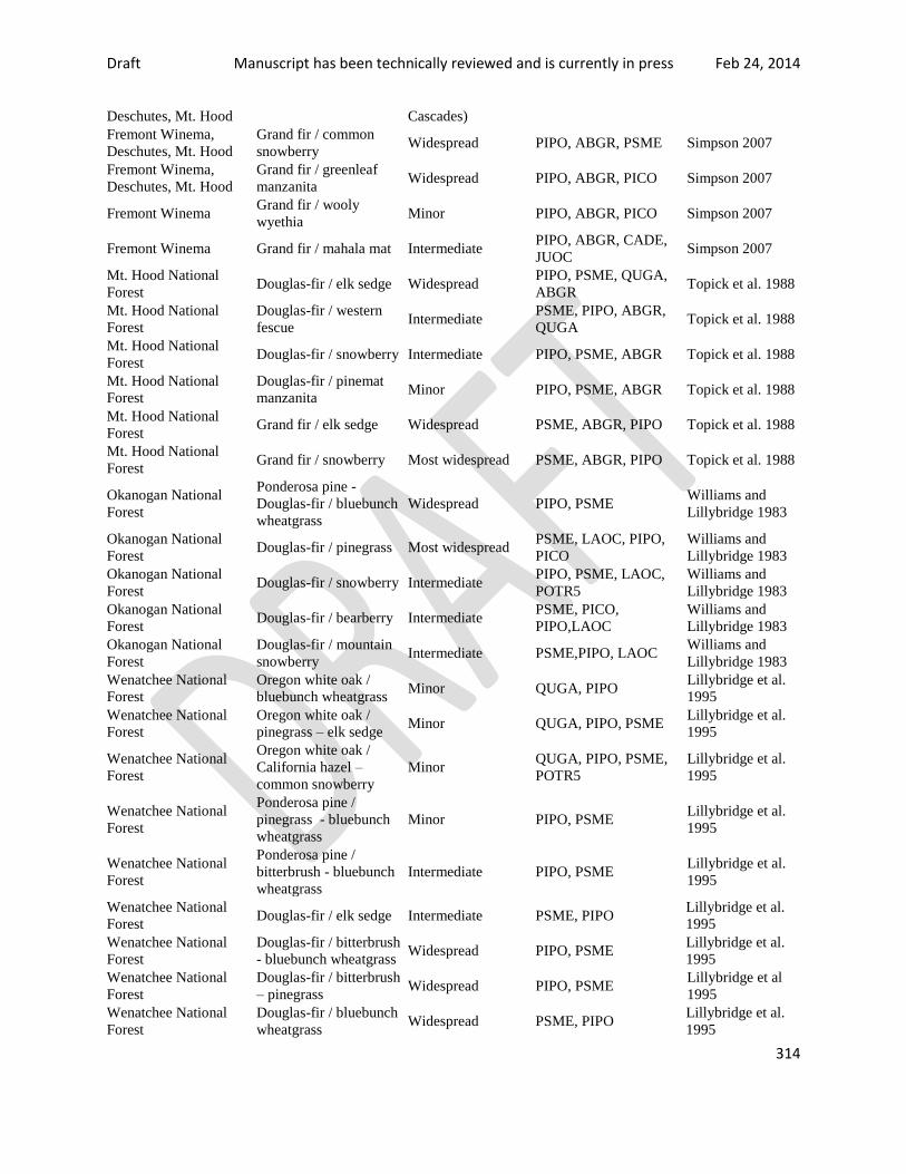
Draft Manuscript has been technically reviewed and is currently in press Feb 24, 2014
314
Deschutes, Mt. Hood Cascades)
Fremont Winema,
Deschutes, Mt. Hood
Grand fir / common
snowberry Widespread PIPO, ABGR, PSME Simpson 2007
Fremont Winema,
Deschutes, Mt. Hood
Grand fir / greenleaf
manzanita Widespread PIPO, ABGR, PICO Simpson 2007
Fremont Winema Grand fir / wooly
wyethia Minor PIPO, ABGR, PICO Simpson 2007
Fremont Winema Grand fir / mahala mat Intermediate PIPO, ABGR, CADE,
JUOC Simpson 2007
Mt. Hood National
Forest Douglas-fir / elk sedge Widespread
PIPO, PSME, QUGA,
ABGR Topick et al. 1988
Mt. Hood National
Forest
Douglas-fir / western
fescue Intermediate
PSME, PIPO, ABGR,
QUGA Topick et al. 1988
Mt. Hood National
Forest Douglas-fir / snowberry Intermediate PIPO, PSME, ABGR Topick et al. 1988
Mt. Hood National
Forest
Douglas-fir / pinemat
manzanita Minor PIPO, PSME, ABGR Topick et al. 1988
Mt. Hood National
Forest Grand fir / elk sedge Widespread PSME, ABGR, PIPO Topick et al. 1988
Mt. Hood National
Forest Grand fir / snowberry Most widespread PSME, ABGR, PIPO Topick et al. 1988
Okanogan National
Forest
Ponderosa pine -
Douglas-fir / bluebunch
wheatgrass
Widespread PIPO, PSME Williams and
Lillybridge 1983
Okanogan National
Forest Douglas-fir / pinegrass Most widespread
PSME, LAOC, PIPO,
PICO
Williams and
Lillybridge 1983
Okanogan National
Forest Douglas-fir / snowberry Intermediate
PIPO, PSME, LAOC,
POTR5
Williams and
Lillybridge 1983
Okanogan National
Forest Douglas-fir / bearberry Intermediate
PSME, PICO,
PIPO,LAOC
Williams and
Lillybridge 1983
Okanogan National
Forest
Douglas-fir / mountain
snowberry Intermediate PSME,PIPO, LAOC
Williams and
Lillybridge 1983
Wenatchee National
Forest
Oregon white oak /
bluebunch wheatgrass Minor QUGA, PIPO
Lillybridge et al.
1995
Wenatchee National
Forest
Oregon white oak /
pinegrass – elk sedge Minor QUGA, PIPO, PSME
Lillybridge et al.
1995
Wenatchee National
Forest
Oregon white oak /
California hazel –
common snowberry
Minor QUGA, PIPO, PSME,
POTR5
Lillybridge et al.
1995
Wenatchee National
Forest
Ponderosa pine /
pinegrass - bluebunch
wheatgrass
Minor PIPO, PSME Lillybridge et al.
1995
Wenatchee National
Forest
Ponderosa pine /
bitterbrush - bluebunch
wheatgrass
Intermediate PIPO, PSME Lillybridge et al.
1995
Wenatchee National
Forest Douglas-fir / elk sedge Intermediate PSME, PIPO
Lillybridge et al.
1995
Wenatchee National
Forest
Douglas-fir / bitterbrush
- bluebunch wheatgrass Widespread PIPO, PSME
Lillybridge et al.
1995
Wenatchee National
Forest
Douglas-fir / bitterbrush
– pinegrass Widespread PIPO, PSME
Lillybridge et al
1995
Wenatchee National
Forest
Douglas-fir / bluebunch
wheatgrass Widespread PSME, PIPO
Lillybridge et al.
1995

Draft Manuscript has been technically reviewed and is currently in press Feb 24, 2014
315
Wenatchee National
Forest
Douglas-fir / pinegrass -
bluebunch wheatgrass Intermediate PIPO, PSME
Lillybridge et al.
1995
Wenatchee National
Forest Douglas-fir / pinegrass widespread
PSME, PIPO, PICO,
LAOC
Lillybridge et al.
1995
Wenatchee National
Forest
Douglas-fir / snowberry
- bluebunch wheatgrass Intermediate PSME, PIPO
Lillybridge et al.
1995
Wenatchee National
Forest
Douglas-fir / snowberry
– pinegrass Widespread PSME, PIPO
Lillybridge et al.
1995
Wenatchee National
Forest Douglas-fir / snowberry Widespread PSME, PIPO
Lillybridge et al
1995
Wenatchee National
Forest
Douglas-fir / mountain
snowberry Intermediate PIPO, PSME
Lillybridge et al.
1995
Wenatchee National
Forest
Douglas-fir / shiny-leaf
spirea – pinegrass Widespread PSME, PIPO
Lillybridge et al.
1995
Wenatchee National
Forest Grand fir / pinegrass Most widespread
PSME, PIPO, ABGR,
PICO
Lillybridge et al.
1995
Wenatchee National
Forest
Grand fir / mountain
snowberry Minor PSME, PIPO, ABGR
Lillybridge et al.
1995
Wenatchee National
Forest
Grand fir / pinemat
manzanita Widespread
PSME, PIPO, ABGR,
PICO, LAOC
Lillybridge et al.
1995
Warm Springs Indian
Reservation
Ponderosa Pine-
Douglas-fir / bitterbrush Intermediate PSME, PIPO CADE Marsh et. al 1987
Warm Springs Indian
Reservation
Ponderosa Pine-
Douglas-fir / bitterbrush-
ceanothus
Widespread PIPO, PSME, CADE Marsh et. al 1987
Warm Springs Indian
Reservation
Ponderosa Pine-
Douglas-fir / snowberry Intermediate PSME, PIPO CADE Marsh et. al 1987
Warm Springs Indian
Reservation
Ponderosa Pine-
Douglas-fir / bitterbrush
(Mutton)
Intermediate PIPO, JUOC, QUGA Marsh et. al 1987
Warm Springs Indian
Reservation
Ponderosa Pine-
Douglas-fir/snowberry
(Mutton)
Intermediate PSME, PIPO CADE Marsh et. al 1987
Warm Springs Indian
Reservation
Ponderosa Pine-
Douglas-fir / greenleaf
manzanita – ceanothus
(Mutton)
Intermediate PSME, PIPO, CADE,
QUGA Marsh et. al 1987
Warm Springs Indian
Reservation
Ponderosa Pine-
Douglas-fir / snowberry
(Mutton)
Intermediate PSME, PIPO QUGA Marsh et. al 1987
Warm Springs Indian
Reservation
Ponderosa Pine-
Douglas-fir / prairie
smoke avens – mule’s
ears (Mutton)
Intermediate PIPO, PSME, JUOC,
QUGA Marsh et. al 1987
Moist-dry with low- to mixed-severity fire—Characterized by low to moderate-severity fire with intervals
intermediate between the dry and moist group. Large high-severity fires rarely occur. Natural fire regimes in order
of prevalence are III A, III B, I, IIIC, and IV A.
Blue and Ochoco
Mountains Douglas-fir / oceanspray Intermediate PSME, PIPO
Johnson and
Clausnitzer 1992
Blue and Ochoco
Mountains
Grand fir / grouse
huckleberry Intermediate
ABGR, LAOC, PSME,
LAOC, PICO PIPO
Johnson and
Clausnitzer 1992
Blue and Ochoco
Mountains
Douglas-fir / Rocky
Mountain Maple- Intermediate PSME, PIPO
Johnson and
Simon 1987

Draft Manuscript has been technically reviewed and is currently in press Feb 24, 2014
316
Wallowa-Snake
Province
mallow ninebark
Blue and Ochoco
Mountains
Wallowa-Snake
Province
Douglas-fir / big
huckleberry Intermediate PSME, PIPO, LAOC
Johnson and
Clausnitzer 1992
Johnson and
Simon 1987
Blue and Ochoco
Mountains Strawberry
Mountains
Douglas-fir / pinemat
manzanita / elk sedge Minor PSME, PIMO, ABLA
Johnson 2004
Blue and Ochoco
Mountains
Wallowa-Snake
Province
Douglas-fir /mallow
ninebark Widespread PSME, PIPO, LAOC
Johnson and
Clausnitzer 1992
Colville National Forest Douglas-fir / ninebark Most widespread PSME, PIPO Williams et al.
1995
Colville National Forest Douglas-fir / ninebark -
twinflower Widespread PSME, LAOC, PIPO
Williams et al.
1995
Colville National Forest Douglas-fir / big
huckleberry Intermediate PSME, LAOC, PICO
Williams et al.
1995
Colville National Forest Douglas-fir / dwarf
huckleberry Minor
PSME, PICO,
LAOC,PIPO, PIEN
Williams et al.
1995
Colville National Forest Grand fir / ninebark Widespread PSME, LAOC, PIPO,
ABGR
Williams et al.
1995
Colville National Forest Grand fir / dwarf
huckleberry Minor
PICO, PSME, LAOC,
ABGR
Williams et al.
1995
Deschutes, Mt. Hood Douglas-fir / chinquapin Widespread PSME, PIPO, CADE,
PILA Simpson 2007
Deschutes, Mt. Hood Douglas-fir / oceanspray Minor PSME, PIPO, QUGA,
JUOC Simpson 2007
Deschutes, Mt. Hood Grand fir / oceanspray Intermediate PSME, PIPO, ABGR Simpson 2007
Fremont Winema,
Deschutes, Mt. Hood Douglas-fir / starflower Widespread PSME, PIPO, CADE
Simpson 2007
Fremont Winema,
Deschutes, Mt. Hood
Douglas-fir / creeping
snowberry Intermediate
PSME, PIPO, CADE,
QUGA Simpson 2007
Fremont Winema,
Deschutes, Mt. Hood
Douglas-fir / prince's
pine Intermediate PSME, PIPO, CADE
Simpson 2007
Fremont Winema Grand fir / creeping
snowberry Intermediate
PIPO, ABGR, PICO,
PSME Simpson 2007
Fremont Winema,
Deschutes, Mt. Hood
Grand fir / golden
chinquapin Widespread PSME, PIPO, ABGR
Simpson 2007
Fremont Winema,
Deschutes, Mt. Hood
Grand fir / western
starflower Widespread PSME, ABGR, PIPO
Simpson 2007
Fremont Winema,
Deschutes, Mt. Hood
Grand fir / common
prince's pine Widespread
PIPO, ABGR, PICO,
PSME Simpson 2007
Fremont Winema,
Deschutes, Mt. Hood
Grand fir / starry false-
solomonseal Widespread PIPO, ABGR, PICO
Simpson 2007
Mt. Hood National
Forest
Douglas-fir / oceanspray
/ elk sedge Widespread
PSME, PIPO, QUGA,
ABGR Topick et al. 1988
Mt. Hood National
Forest Grand fir /starflower Widespread PSME, ABGR, PIPO
Topick et al. 1988
Fremont Winema,
Deschutes, Mt. Hood
Grand fir / long-stolen
sedge Intermediate PIPO, PICO, ABGR
Simpson 2007
Fremont Winema, Grand fir / pinemat Intermediate ABCO, PICO, PIPO, Simpson 2007

Draft Manuscript has been technically reviewed and is currently in press Feb 24, 2014
317
Deschutes, Mt. Hood manzanita PIMO
Mt. Hood National
Forest Grand fir / chinkquapin Minor
ABGR, PSME, PICO,
LAOC, PIPO Topick et al. 1988
Okanogan National
Forest Douglas-fir / ninebark Minor
PSME, LAOC, PICO,
PIPO
Williams and
Lillybridge 1983
Okanogan National
Forest Douglas-fir / boxwood Minor PSME, PIPO, POTR5
Williams and
Lillybridge 1983
Okanogan National
Forest
Douglas-fir /
huckleberry Intermediate
PSME, LAOC, PICO,
PIPO
Williams and
Lillybridge 1983
Okanogan National
Forest Subalpine fir / pinegrass Intermediate
PSME, ABLA,PICO,
LAOC, PIPO
Williams and
Lillybridge 1983
Wenatchee National
Forest
Douglas-fir /
huckleberry (3 minor
huckleberry
associations)
Minor PSME, LAOC, PICO,
PIPO Lillybridge et al.
1995
Wenatchee National
Forest
Grand fir / pinegrass -
lupine Intermediate
PSME, PIPO, ABGR,
PICO, LAOC
Lillybridge et al.
1995
Wenatchee National
Forest
Grand fir / heartleaf
arnica Intermediate
PSME, ABGR, LAOC,
PIPO, PIEN
Lillybridge et al.
1995
Wenatchee National
Forest
Grand fir / oceanspray -
pinegrass Intermediate
PSME, ABGR, PIPO,
LAOC
Lillybridge et al.
1995
Wenatchee National
Forest
Grand fir / Cascade
Oregon grape -
pinegrass
Intermediate PSME, ABGR, PICO,
LAOC, PIPO Lillybridge et al.
1995
Wenatchee National
Forest
Grand fir / common
snowberry - pinegrass Intermediate PSME, ABGR, PIPO
Lillybridge et al.
1995
Warm Springs Indian
Reservation
Mixed Conifer /
snowberry / elk sedge Intermediate PIPO, PSME, ABGR
Marsh et. al 1987
Warm Springs Indian
Reservation
Mixed Conifer /
ceanothus Widespread
PIPO, PSME, ABGR,
CADE Marsh et. al 1987
Warm Springs Indian
Reservation
Mixed Conifer /
snowberry Widespread PSME, PIPO ABGR
Marsh et. al 1987
Warm Springs Indian
Reservation
Mixed Conifer /
boxwood Intermediate
ABGR, PSME, PIPO,
LAOC Marsh et. al 1987
Warm Springs Indian
Reservation Grand fir / boxwood Intermediate
ABGR, PSME, PIPO,
LAOC Marsh et. al 1987
Moist with mixed-severity fire—Characterized by moderate to high-severity fire with lesser amounts of low-
severity fire in comparison to the moist-dry group. Fire return intervals are usually longer than 50 years. Natural fire
regimes in order of prevalence are III B, III C, III A, IV B, and IV A.
Blue and Ochoco
Mountains
Wallowa-Snake
Province
Grand fir / big
huckleberry Widespread
ABGR, LAOC, PSME,
PIEN, ABLA, PIPO,
PICO
Johnson and
Clausnitzer 1992
Johnson and
Simon 1987
Blue and Ochoco
Mountains
Wallowa-Snake
Province
Grand fir / Rocky
Mountain maple Intermediate
ABGR, PIEN, PSME,
LAOC, PIMO,
Johnson and
Clausnitzer 1992
Johnson and
Simon 1987
Blue and Ochoco
Mountains
Grand fir / Columbia
brome Intermediate
ABGR, PSME, LAOC,
PIEN
Johnson and
Clausnitzer 1992
Blue and Ochoco
Mountains
Grand fir / grouse
huckleberry -
twinflower
Intermediate ABGR, PIEN, LAOC,
PSME,
Johnson and
Clausnitzer 1992
Blue and Ochoco Grand fir / twinflower Widespread ABGR, PIEN, PSME, Johnson and
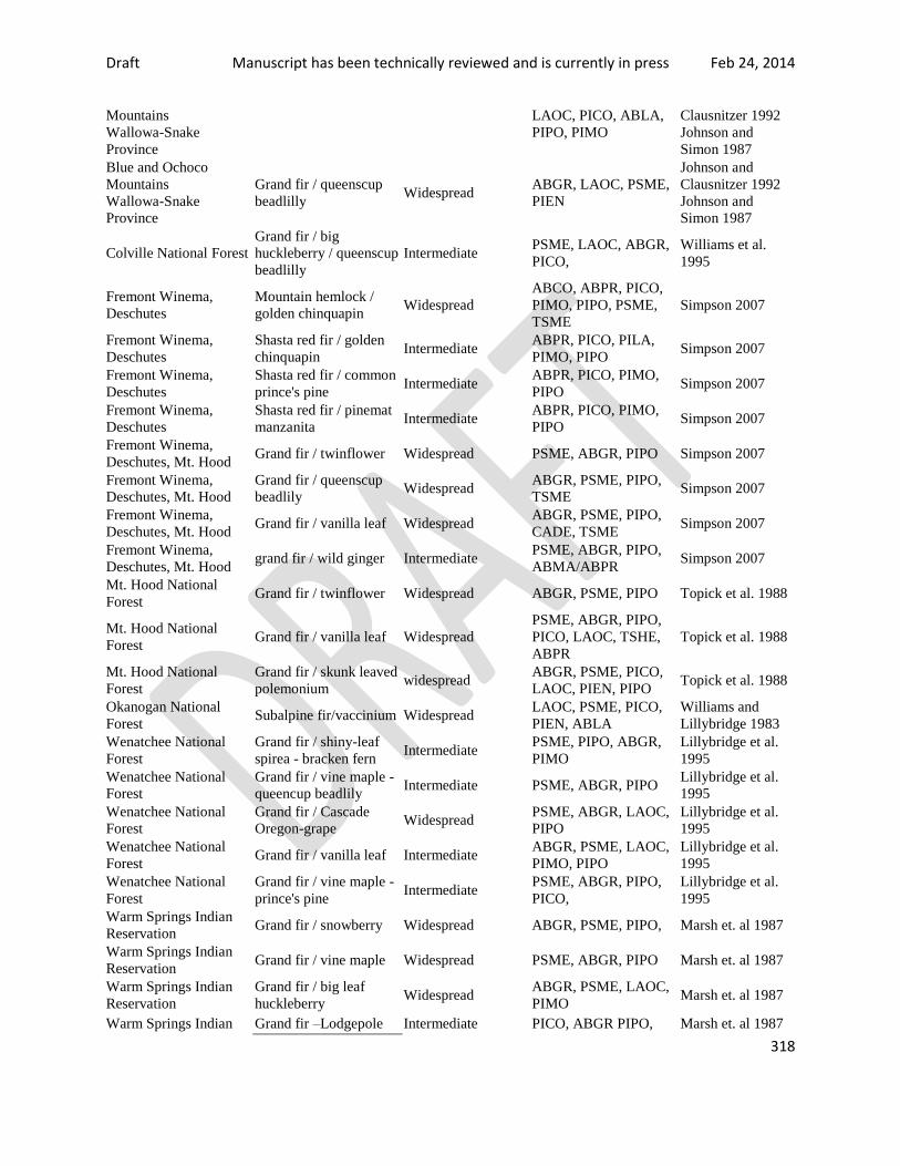
Draft Manuscript has been technically reviewed and is currently in press Feb 24, 2014
318
Mountains
Wallowa-Snake
Province
LAOC, PICO, ABLA,
PIPO, PIMO
Clausnitzer 1992
Johnson and
Simon 1987
Blue and Ochoco
Mountains
Wallowa-Snake
Province
Grand fir / queenscup
beadlilly Widespread
ABGR, LAOC, PSME,
PIEN
Johnson and
Clausnitzer 1992
Johnson and
Simon 1987
Colville National Forest
Grand fir / big
huckleberry / queenscup
beadlilly
Intermediate PSME, LAOC, ABGR,
PICO,
Williams et al.
1995
Fremont Winema,
Deschutes
Mountain hemlock /
golden chinquapin Widespread
ABCO, ABPR, PICO,
PIMO, PIPO, PSME,
TSME
Simpson 2007
Fremont Winema,
Deschutes
Shasta red fir / golden
chinquapin Intermediate
ABPR, PICO, PILA,
PIMO, PIPO Simpson 2007
Fremont Winema,
Deschutes
Shasta red fir / common
prince's pine Intermediate
ABPR, PICO, PIMO,
PIPO Simpson 2007
Fremont Winema,
Deschutes
Shasta red fir / pinemat
manzanita Intermediate
ABPR, PICO, PIMO,
PIPO Simpson 2007
Fremont Winema,
Deschutes, Mt. Hood Grand fir / twinflower Widespread PSME, ABGR, PIPO Simpson 2007
Fremont Winema,
Deschutes, Mt. Hood
Grand fir / queenscup
beadlily Widespread
ABGR, PSME, PIPO,
TSME Simpson 2007
Fremont Winema,
Deschutes, Mt. Hood Grand fir / vanilla leaf Widespread
ABGR, PSME, PIPO,
CADE, TSME Simpson 2007
Fremont Winema,
Deschutes, Mt. Hood grand fir / wild ginger Intermediate
PSME, ABGR, PIPO,
ABMA/ABPR Simpson 2007
Mt. Hood National
Forest Grand fir / twinflower Widespread ABGR, PSME, PIPO Topick et al. 1988
Mt. Hood National
Forest Grand fir / vanilla leaf Widespread
PSME, ABGR, PIPO,
PICO, LAOC, TSHE,
ABPR
Topick et al. 1988
Mt. Hood National
Forest
Grand fir / skunk leaved
polemonium widespread
ABGR, PSME, PICO,
LAOC, PIEN, PIPO Topick et al. 1988
Okanogan National
Forest Subalpine fir/vaccinium Widespread
LAOC, PSME, PICO,
PIEN, ABLA
Williams and
Lillybridge 1983
Wenatchee National
Forest
Grand fir / shiny-leaf
spirea - bracken fern Intermediate
PSME, PIPO, ABGR,
PIMO
Lillybridge et al.
1995
Wenatchee National
Forest
Grand fir / vine maple -
queencup beadlily Intermediate PSME, ABGR, PIPO
Lillybridge et al.
1995
Wenatchee National
Forest
Grand fir / Cascade
Oregon-grape Widespread
PSME, ABGR, LAOC,
PIPO
Lillybridge et al.
1995
Wenatchee National
Forest Grand fir / vanilla leaf Intermediate
ABGR, PSME, LAOC,
PIMO, PIPO
Lillybridge et al.
1995
Wenatchee National
Forest
Grand fir / vine maple -
prince's pine Intermediate
PSME, ABGR, PIPO,
PICO,
Lillybridge et al.
1995
Warm Springs Indian
Reservation Grand fir / snowberry Widespread ABGR, PSME, PIPO, Marsh et. al 1987
Warm Springs Indian
Reservation Grand fir / vine maple Widespread PSME, ABGR, PIPO Marsh et. al 1987
Warm Springs Indian
Reservation
Grand fir / big leaf
huckleberry Widespread
ABGR, PSME, LAOC,
PIMO Marsh et. al 1987
Warm Springs Indian Grand fir –Lodgepole Intermediate PICO, ABGR PIPO, Marsh et. al 1987

Draft Manuscript has been technically reviewed and is currently in press Feb 24, 2014
319
Reservation pine/ boxwood /
pinegrass
ABLA,
Moist to wet with high-severity fire—Higher severity fire tends to dominate in most events and return intervals are
usually greater than 100 years. Natural fire regimes in order of prevalence are III C, and IV B.
Blue and Ochoco
Mountains Grand fir / Oakfern Minor
ABGR, PIEN, PSME,
LAOC, ACGL, TABR
Johnson and
Clausnitzer 1992
Blue and Ochoco
Mountains
Grand fir / sword fern –
ginger Intermediate
ABGR, PSME, LAOC,
PIEN
Johnson and
Clausnitzer 1992
Blue and Ochoco
Mountains
Wallowa-Snake
Province
Grand fir / Pacific yew/
queen's cup beadlilly Intermediate
ABGR, PIEN, PSME,
LAOC, TABR
Johnson and
Clausnitzer 1992
Johnson and
Simon 1987
Blue and Ochoco
Mountains
Grand fir / Pacific yew/
twinflower minor
ABGR, PSME, LAOC,
PIEN, TABR
Johnson and
Clausnitzer 1992
Blue and Ochoco
Mountains
Grand fir / false
bugbane Intermediate
ABGR, PIEN, ABLA,
LAOC, PICO, TABR
Johnson and
Clausnitzer 1992
Colville National Forest
Grand fir / Douglas
maple / queencup
beadlilly
Intermediate PSME, LAOC, ABGR Williams et al.
1995
Mt. Hood National
Forest
Grand fir - Engelmann
spruce / starry
solomonplume
Minor ABGR, PIEN, PSME,
PICO Topick et al. 1988
Mt. Hood National
Forest
Grand fir / vanilla leaf -
vine maple Widespread
PSME, PIPO, ABGR,
CONU Topick et al. 1988
This is intended as an interim classification subject to further revision as new information becomes available. Note 1
that terms used to describe climatic environment are relative terms, and have different definitions among regions. 2
Therefore this regional classification may differ from local classifications. 3
4
*Description of table columns 5
National Forest/Region—Describes the subregion of the plant association. 6
Extent—Describes the geographic distribution and approximate area of a plant association relative to other 7
associations within the region. 8
Species composition—All tree species recorded in each association all listed ordered by prominence within each 9
association. 10
Source—Citation for plant association description. 11
Acronym Species Acronym Species
ABGR Abies grandis (Grand fir) PIEN Picea engelmannii (Engelmann spruce)
ABLA Abies lasiocarpa (subalpine fir) PILA Pinus lambertiana (sugar pine)
ABPR Abies procera (noble fir) PIMO Pinus monticola (western white pine)

Draft Manuscript has been technically reviewed and is currently in press Feb 24, 2014
320
ACGL Acer glabrum (Rocky Mountain maple) PIPO Pinus ponderosa (ponderosa pine)
CADE Calocedrus decurrens (incense cedar) PSME Pseudotsuga menziesii (Douglas-fir)
CONU Cornus nutallii (Pacific dogwood) QUGA Quercus garryana (Oregon white oak)
JUOC Juniperus occidentalis (western juniper) TABR Taxus brevifolia (Pacific yew)
LAOC Larix occidentalis (western larch) TSHE Tsuga heterophylla (western hemlock)
PICO Pinus contorta (lodgepole pine) TSME Tsuga mertensiana (mountain hemlock)
1
2

Draft Manuscript has been technically reviewed and is currently in press Feb 24, 2014
321
Table 3—Historical and current density (trees per hectare) of large diameter (typically >50
cm) trees in dry and moist mixed-conifer forest
Region
Forest
description
Historical
density
Current density Source Notes
Mean +- standard deviation (range)
and time period
Eastern
Slope of the
Cascades,
Southern
OR.
Mixed-dry
35 ± 15 (3-105)
1914-1922
21 ± 12 (0-45)
1997-2006
Hagmann et
al. 2013
Historical density is reported for trees
>53 cm diameter at breast height
(DBH) based on timber inventory
transects that covered 10-20 percent
(6,646 ha) of a 38,641-ha study area of
ponderosa pine and dry and moist
mixed-conifer forest. Current density is
based on 24 current vegetation survey
(CVS) plots within the study area, and
density is reported for all trees >53 cm
DBH. Inventory plots were assigned to
habitat types (dry or moist) using
mapped potential vegetation types
(ILAP).
Mixed-moist
35 ± 17 (3-147)
1914-1922
16 ± 15 (0-114)
1997-2006
Warm
Springs
Indian
Reservation,
Eastern
Slope of the
Cascades,
OR.
Mixed-dry
24 ± 10 (1-62)
1922-1925
NA
Hagmann,
unpublished
data, 2013
Historical density is reported for trees
>53 cm DBH based on timber
inventory transects. Plot size varied by
species. Transects covered >20 percent
(6,952-11,327 ha) of a 32,293-ha study
area of dry and MMC forest. Inventory
plots were assigned to habitat types
using mapped potential vegetation
types (ILAP).
Mixed-moist
26 ± 12 (0-102)
1922-1925
NA
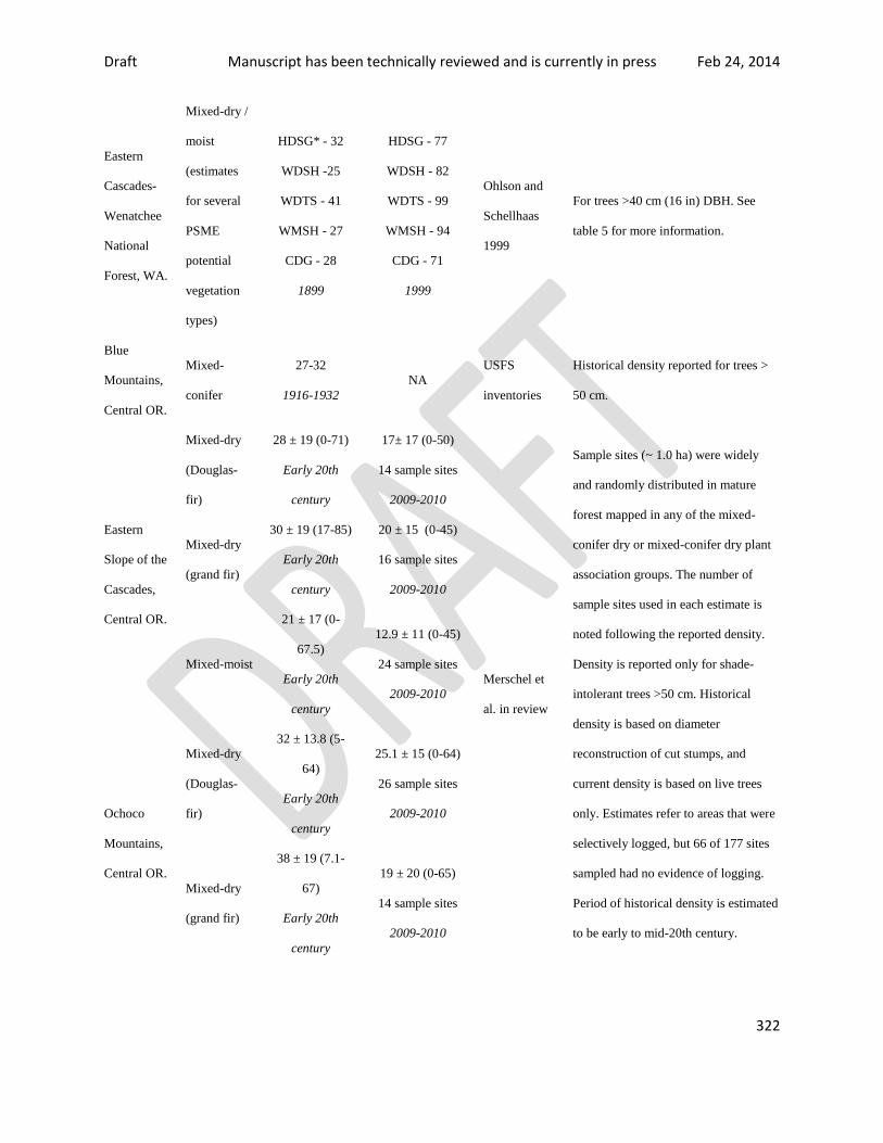
Draft Manuscript has been technically reviewed and is currently in press Feb 24, 2014
322
Eastern
Cascades-
Wenatchee
National
Forest, WA.
Mixed-dry /
moist
(estimates
for several
PSME
potential
vegetation
types)
HDSG* - 32
WDSH -25
WDTS - 41
WMSH - 27
CDG - 28
1899
HDSG - 77
WDSH - 82
WDTS - 99
WMSH - 94
CDG - 71
1999
Ohlson and
Schellhaas
1999
For trees >40 cm (16 in) DBH. See
table 5 for more information.
Blue
Mountains,
Central OR.
Mixed-
conifer
27-32
1916-1932
NA
USFS
inventories
Historical density reported for trees >
50 cm.
Eastern
Slope of the
Cascades,
Central OR.
Mixed-dry
(Douglas-
fir)
28 ± 19 (0-71)
Early 20th
century
17± 17 (0-50)
14 sample sites
2009-2010
Merschel et
al. in review
Sample sites (~ 1.0 ha) were widely
and randomly distributed in mature
forest mapped in any of the mixed-
conifer dry or mixed-conifer dry plant
association groups. The number of
sample sites used in each estimate is
noted following the reported density.
Density is reported only for shade-
intolerant trees >50 cm. Historical
density is based on diameter
reconstruction of cut stumps, and
current density is based on live trees
only. Estimates refer to areas that were
selectively logged, but 66 of 177 sites
sampled had no evidence of logging.
Period of historical density is estimated
to be early to mid-20th century.
Mixed-dry
(grand fir)
30 ± 19 (17-85)
Early 20th
century
20 ± 15 (0-45)
16 sample sites
2009-2010
Mixed-moist
21 ± 17 (0-
67.5)
Early 20th
century
12.9 ± 11 (0-45)
24 sample sites
2009-2010
Ochoco
Mountains,
Central OR.
Mixed-dry
(Douglas-
fir)
32 ± 13.8 (5-
64)
Early 20th
century
25.1 ± 15 (0-64)
26 sample sites
2009-2010
Mixed-dry
(grand fir)
38 ± 19 (7.1-
67)
Early 20th
century
19 ± 20 (0-65)
14 sample sites
2009-2010

Draft Manuscript has been technically reviewed and is currently in press Feb 24, 2014
323
Mixed-moist
18 ± 16 (0-48)
Early 20th
century
13 ± 13 (0-40)
14 sample sites
2009-2010
Blue
Mountains,
Eastern OR.
Mixed-
conifer
NA
38 TPH
2012
Johnston,
unpublished
data 2013
Density is reported for trees >50 cm in
unlogged areas and provides an
estimate of historical large tree density
in logged areas in dry and MMC
forests.
Eastern
Cascades
Slope and
Foothills,
OR and
WA.
Mixed-dry NA
21 ± 23 (n=512)
1994-2004
Reilly 2012,
unpublished
data
Density based on forest CVS plots
distributed on a 2.5 by 2.5 km grid (5
km in Wilderness Areas) throughout
national forest of OR and WA. Sample
sites include developmental stages
ranging from early seral in recently
disturbed areas (logging, wildfire, etc.)
to mature old-growth forest. Density
estimates are reported for trees >50 cm
DBH. The number of CVS plots used
to calculate density is reported in
parentheses. CVS plots were assigned
to PVTs based on ILAP.
Mixed-moist NA
27 ± 27 (n=280)
1994-2004
Blue
Mountains
ecoregion,
OR and
WA.
Mixed-dry NA
19 ± 16 (n=471)
1994-2004
Mixed-moist NA
23 ± 21 (n=1041)
1994-2004
See table 5 caption for more information. Diameter thresholds, methods of estimation, and spatial 1
coverage used to develop estimates varies among authors. 2
*Plant Association Groups with respective Plant Associations 3 HDSG (Hot/Dry/Shrub/Grass) 4 Pinus ponderosa/Agropyron spicatum 5 Pseudotsuga menziesii/Agropyron spicatum 6 Pinus ponderosa/Purshia tridentata/Agropyron spicatum 7 Pseudotsuga menziesii/Purshia tridentata/Agropyron spicatum 8 Pseudotsuga menziesii/Symphoricarpos albus/Agropyron spicatum 9 WDSH (Warm/Dry/Shrub/Herb) 10 Pseudotsuga menziesii/Arctostaphylos uva-ursi 11 Pseudotsuga menziesii/Arctostaphylos uva-ursi/Purshia tridentata 12 Pseudotsuga menziesii/Spirea betulifolia var. lucida 13 WDTS (Warm/Dry/Tall Shrub) 14 Pseudotsuga menziesii/Physocarpus malvaceus 15 Pseudotsuga menziesii/Physocarpus malvaceus/Linaea borealis var. longiflora 16

Draft Manuscript has been technically reviewed and is currently in press Feb 24, 2014
324
WMSH (Warm/Mesic/Shrub/Herb) 1 Pseudotsuga menziesii/Symphoricarpos albus 2 Pseudotsuga menziesii/Symphoricarpos albus/Calamagrostis rubescens 3 CDG (Cool/Dry/Grass) 4 Pseudotsuga menziesii/Arctostaphylos uva-ursi/Calamagrostis rubescens 5 Pseudotsuga menziesii/Purshia tridentata/Calamagrostis rubescens 6 Pseudotsuga menziesii/Spirea betulifolia var. lucida/Calamagrostis rubescens 7
8

Draft Manuscript has been technically reviewed and is currently in press Feb 24, 2014
325
Table 4—Insects considered major disturbances in moist mixed-conifer forests of eastern Oregon 1
and Washington 2
Common
name
Scientific
name
Primary host(s)
in region
Scale of
outbreaks
Impacts
Bark beetles
Douglas-fir
beetle
Dendroctonus
pseudotsugae
Douglas-fir
Local to
landscape
Mortality of individual trees or small
groups of trees is typically associated
with defoliation, drought, windthrow,
wildfire, or root disease. Once
established, outbreaks may cause
large amounts of tree mortality over
extensive areas.
fir engraver
Scolytus
ventralis
grand fir, white
fir
Local to
landscape
Mortality of individual trees or small
groups of trees is typically associated
with drought and defoliation. Once
established, outbreaks may cause
large amounts of tree mortality.
mountain pine
beetle
Dendroctonus
ponderosae
lodgepole pine,
ponderosa pine,
western white
pine
Local to
regional
Episodic outbreaks are a common
occurrence, but the magnitude and
extent of recent outbreaks have
exceeded the range of historic
variability in much of the western
U.S.
western balsam Dryocoetes grand fir, Local to Mortality of individual trees or small

Draft Manuscript has been technically reviewed and is currently in press Feb 24, 2014
326
bark beetle
confusus subalpine fir landscape groups of trees is common and
associated with windthrow.
Defoliators and other
balsam woolly
adelgid
Adelges
piceae
Grand fir, silver
fir, subalpine fir
Local
Accidentally introduced into the U.S.
from Europe and first detected in the
Pacific Northwest in 1929. Adelgids
are sap-sucking insects. Feeding
causes abnormal growth responses in
affected trees termed “rotholtz.”
Severe infestations cause growth
loss, top-kill and tree mortality.
Douglas-fir
tussock moth
Orgyia
pseudotsugata
Douglas-fir,
grand fir, white
fir, subalpine fir
Local to
regional
Larval feeding causes growth loss,
top-kill and tree mortality. Outbreaks
are often short-lived.
larch
casebearer
Coleophora
laricella
western larch Local
Accidentally introduced into the U.S.
from Europe and first detected in the
Pacific Northwest in the 1950s.
Larvae mine needles. Severe
defoliation occurs, but larch (a
deciduous conifer) withstands
repeated defoliation. Growth loss is
common, but tree mortality is rare.

Draft Manuscript has been technically reviewed and is currently in press Feb 24, 2014
327
western spruce
budworm
Choristoneura
occidentalis
Douglas-fir,
grand fir, white
fir, subalpine fir,
western larch
Local to
regional
Early instar larvae mine needles and
buds. Late instar larval feeding
causes growth loss, top-kill, and tree
mortality. Feeding on staminate
flowers and conelets affects
regeneration.
1
2

Draft Manuscript has been technically reviewed and is currently in press Feb 24, 2014
328
Table 5—Historical and current tree density (trees per hectare, TPH) estimates in dry and moist 1
mixed-conifer forests 2
Region
Forest
description
Historical
density
Current
density
Source Notes
Mean +- standard deviation (range)
and time period
Eastern
Slope of the
Cascades,
Southern
OR.
Mixed-Dry
64 ± 22
(14-156)
1914-1922
286 ± 130
(109-572)
1997-2006
Hagmann
et al. 2013
Historical density is
reported for trees >15.2
cm DBH based on timber
inventory transects that
covered 10-20 percent
(6,646 ha) of a 38,641 ha
study area of ponderosa
pine and dry and moist
mixed-conifer forest.
Current density is reported
for trees >15 cm DBH and
is based on 24 current
vegetation survey plots
within the sample area.
Inventory plots were
assigned to habitat types
using mapped potential
vegetation types (ILAP).
Mixed-
Moist
78 ± 37
(0-296)
1914-1922
233 ± 90
(104-378)
1997-2006

Draft Manuscript has been technically reviewed and is currently in press Feb 24, 2014
329
Warm
Springs
Indian
Reservation,
Eastern
Slope of the
Cascades,
OR.
Mixed-Dry
65 ± 25
(6-188)
1922-1925
NA
Hagmann,
unpublish
ed data,
2013
Historical density is
reported for trees >15.2
cm DBH based on timber
inventory transects that
covered 20 percent
(32,293 ha) of a 158,354
ha study area of dry and
moist mixed-conifer
forest. Inventory plots
were assigned to habitat
types using mapped
potential vegetation types
(ILAP).
Mixed-
Moist
70 ± 32
(0-289)
1922-1925
NA
Austin-
Whitney
Tract in the
Blue
Mountains
of NE OR.
Mixed-Dry
120
1910
NA Munger
1912
(summariz
ed by
David
Powell)
Density is reported for
trees >10 cm DBH.
Munger specifically
inventoried "well stocked"
stands.
Crawford
Creek Tract
in the Blue
Mountains
near Unity,
Mixed-Dry
126
1912
NA

Draft Manuscript has been technically reviewed and is currently in press Feb 24, 2014
330
OR.
Lookinglass
Creek Tract
in the
Wallowa
Mountains
of NE OR.
Mixed-
Moist
162
1910
NA
Eastern
Slope of the
Cascades,
Central OR.
Mixed-Dry
136
1912
NA
Munger
1917
Density is reported for
trees >10 cm DBH.
Munger specifically
inventoried "well stocked"
stands.
Eastern
Slope of the
Cascades,
Central OR.
Mixed-
Conifer
275
late 1800s
NA
Baker
2012
General land office survey
records were used to
estimate stand density.
Estimates for a 398,346 ha
area are based on 11,856
trees marking section and
quarter section corners.
Four trees were used to
estimate density at section
corners, and two were
used at quarter corners.
This inventory area
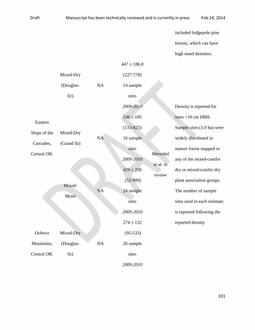
Draft Manuscript has been technically reviewed and is currently in press Feb 24, 2014
331
included lodgepole pine
forests, which can have
high stand densities.
Eastern
Slope of the
Cascades,
Central OR.
Mixed-Dry
(Douglas-
fir)
NA
447 ± 186.8
(227-778)
14 sample
sites
2009-2010
Merschel
et al. in
review
Density is reported for
trees >10 cm DBH.
Sample sites (1.0 ha) were
widely distributed in
mature forest mapped in
any of the mixed-conifer
dry or mixed-conifer dry
plant association groups.
The number of sample
sites used in each estimate
is reported following the
reported density
Mixed-Dry
(Grand fir)
NA
536 ± 185
(113-825)
16 sample
sites
2009-2010
Mixed-
Moist
NA
429 ± 200
(52-900)
24 sample
sites
2009-2010
Ochoco
Mountains,
Central OR.
Mixed-Dry
(Douglas-
fir)
NA
274 ± 132
(95-533)
26 sample
sites
2009-2010

Draft Manuscript has been technically reviewed and is currently in press Feb 24, 2014
332
Mixed-Dry
(Grand fir)
NA
203 ± 102
(76-430)
19 sample
sites
2009-2010
Mixed-
Moist
NA
312 ± 211
(67-799)
26 sample
sites
2009-2010
Eastern
Slope of the
Cascades,
Central OR.
Dry and
Moist
Mixed-
Conifer
40-80 in eight
stands, <30 in
5 stands.
Refers to trees
>150 years
old
868
(335-1415)
~2004
Perry et
al. 2004
Age and size were
sampled for live trees at 13
0.2 ha sites. Historic
density refers to the
number of trees per
hectare >150 years in age.
Current density refers to
all trees >5 cm DBH.
Eastern
Slope of the
Cascades, N
WA.
Mixed-
Conifer-Dry
HDSG* - 119
WDSH -168
WDTS - 315
CDG - 311
WMSH - 113
1899
HDSG - 218
WDSH - 326
WDTS - 293
CDG - 376
WMSH - 556
1999
Ohlson
and
Schellhaas
1999
Historical density was
estimated using 52 1/10th
acre plots. Authors suggest
changes in fire regime and
associated changes in
structure began in the

Draft Manuscript has been technically reviewed and is currently in press Feb 24, 2014
333
1860s and that maximum
density was reach in the
mid-20th century.
Historical reconstructed
densities and current
densities are reported for
all trees >12.7 cm DBH,
and are stratified by
different Douglas-fir
potential vegetation types
ranked from most xeric to
most mesic. WMSH
would correspond to moist
mixed-conifer PVTs. It
had a fire return interval of
<19 years. The relatively
high historical density in
WDTS, a type related to a
mixed severity fire that
occurred in 1886.
Eastern
Cascades
Slope and
Foothills,
Mixed-Dry NA
470 ± 267
(n=512)
1994-2004
Matt
Reilly,
unpublish
ed data
Density is reported for
trees >10 cm DBH.
Density based on forest
CVS plots distributed on a

Draft Manuscript has been technically reviewed and is currently in press Feb 24, 2014
334
OR. and
WA.
2.5 by 2.5 km grid (5 km
in Wilderness Areas)
throughout national forest
of Oregon and
Washington. Sample sites
include developmental
stages ranging from early
seral in recently disturbed
areas (logging, wildfire,
etc.) to mature old-growth
forest. The number of
CVS plots used to
calculate density is
reported in parentheses.
CVS plots were assigned
to PVTs based on ILAP
map.
1 2 Note: Dry mixed-conifer forests are included because several studies indicate that historical and current 3 disturbance regimes and stand densities of the two sites overlap to a large degree (see table 2). Diameter 4 thresholds, methods of estimation, and spatial coverage used to develop estimates varies among authors. 5 6 *Plant Association Groups with respective Plant Associations 7 HDSG (Hot/Dry/Shrub/Grass) 8 Pinus ponderosa/Agropyron spicatum 9 Pseudotsuga menziesii/Agropyron spicatum 10 Pinus ponderosa/Purshia tridentata/Agropyron spicatum 11 Pseudotsuga menziesii/Purshia tridentata/Agropyron spicatum 12 Pseudotsuga menziesii/Symphoricarpos albus/Agropyron spicatum 13 WDSH (Warm/Dry/Shrub/Herb) 14 Pseudotsuga menziesii/Arctostaphylos uva-ursi 15 Pseudotsuga menziesii/Arctostaphylos uva-ursi/Purshia tridentata 16 Pseudotsuga menziesii/Spirea betulifolia var. lucida 17 WDTS (Warm/Dry/Tall Shrub) 18

Draft Manuscript has been technically reviewed and is currently in press Feb 24, 2014
335
Pseudotsuga menziesii/Physocarpus malvaceus 1 Pseudotsuga menziesii/Physocarpus malvaceus/Linaea borealis var. longiflora 2 WMSH (Warm/Mesic/Shrub/Herb) 3 Pseudotsuga menziesii/Symphoricarpos albus 4 Pseudotsuga menziesii/Symphoricarpos albus/Calamagrostis rubescens 5 CDG (Cool/Dry/Grass) 6 Pseudotsuga menziesii/Arctostaphylos uva-ursi/Calamagrostis rubescens 7 Pseudotsuga menziesii/Purshia tridentata/Calamagrostis rubescens 8 Pseudotsuga menziesii/Spirea betulifolia var. lucida/Calamagrostis rubescens 9
10

Draft Manuscript has been technically reviewed and is currently in press Feb 24, 2014
336
Table 6—Source forest-habitat trends (1800s to 1995) for families of focal wildlife species in 6th
1
hydrologic unit code (HUC) subwatersheds of the interior Columbia River Basin in eastern Oregon 2
and Washington. Trend was determined by >50 percent of subwatersheds decreasing (-) or 3
increasing (+); otherwise, trend was neutral. 4
Percentage of 6th code watersheds
Province Family name Decreasing Neutral Increasing Trend
Blue Mountains Low-elevation old forest 67 20 13 -
Broad-elevation old forest 47 17 36 0
Forest mosaic 7 15 78 +
Early-seral montane and lower
montane forest 53 4 42 -
Average 43.5 14.0 42.3 0
Northern
Cascades Low-elevation old forest 69 24 7 -
Broad-elevation old forest 74 13 13 -
Forest mosaic 17 45 37 0
Early-seral montane and lower
montane forest 30 8 63 +
Average 47.5 22.5 30.0 0
Southern
Cascades Low-elevation old forest 56 22 22 -
Broad-elevation old forest 37 15 47 0
Forest mosaic 0 20 80 +
Early-seral montane and lower
montane forest 45 13 42 0

Draft Manuscript has been technically reviewed and is currently in press Feb 24, 2014
337
Average 34.5 17.5 47.8 0
Upper Klamath Low-elevation old forest 33 19 48 0
Broad-elevation old forest 7 5 88 +
Forest mosaic 5 7 88 +
Early-seral montane and lower
montane forest 98 0 2 -
Average 35.75 7.75 56.50 0
1
Source: Wisdom et al. (2000). 2
3

Draft Manuscript has been technically reviewed and is currently in press Feb 24, 2014
338
Table 7—Sensitive wildlife species found in interior mesic forests, including species broadly 1
associated with interior moist forest and ecotones. Many of these species are associated with specific 2
forest structure or seral stages found within the interior mesic forest zone. 3
Common name Scientific name Class Status* Comments
Western toad Anaxyrus boreas Amphibian FCo
Rocky mountain tailed
frog
Ascaphus montanus Amphibian FCo
Oregon slender
salamander
Batrachoseps wrighti Amphibian FCo Eastern OR
Cascades
Larch mountain
salamander
Plethodon larselli Amphibian FCo Southeast Cascades
WA
Columbia spotted frog Rana luteiventris Amphibian SC
Northern leopard frog Rana pipiens Amphibian FCo
Oregon spotted frog Rana pretiosa Amphibian FC
Northern goshawk Accipiter gentilis Bird FCo
Upland sandpiper Bartramia longicauda Bird SE
Vaux’s swift Chaetura vauxi Bird SC
Olive-sided flycatcher Contopus cooperi Bird FCo
Black swift Cypseloides niger Bird FCo Associated w/
waterfalls & wet
cliffs
Pileated woodpecker Dryocopus pileatus Bird SC
Peregrine falcon Falco peregrinus Bird FCo
Harlequin duck Histrionicus histrionicus Bird FCo

Draft Manuscript has been technically reviewed and is currently in press Feb 24, 2014
339
Lewis’ woodpecker Melanerpes lewis Bird SC
Flammulated owl Otus flammeolus Bird SC Associated more
with dry forest
White-headed
woodpecker
Picoides albolarvatus Bird FCo Associated more
with dry forest
Black-backed
woodpecker
Picoides arcticus Bird SC
Northern spotted owl Strix occidentalis Bird FT
Silver-bordered fritillary Boloria selene atrocostalis Insect SC
Manns mollusk-eating
ground beetle
Scaphinotus mannii Insect SC
Gray wolf Canis lupus Mammal FE**
Townsend’s big-eared
bat
Corynorhinus townsendii Mammal FCo
Spotted bat Euderma maculatum Mammal FCo
Wolverine Gulo gulo Mammal FC
Silver-haired bat Lasionycteris noctivagans Mammal FCo
Lynx Lynx canadensis Mammal FT
Fisher Martes pennanti Mammal FC Northeast WA, east
of Okanogan River
Long-eared myotis bat Myotis evotis Mammal FCo
Long-legged myotis bat Myotis volans Mammal FCo
Woodland caribou Rangifer tarandus caribou Mammal FE Selkirk Mountain
population in
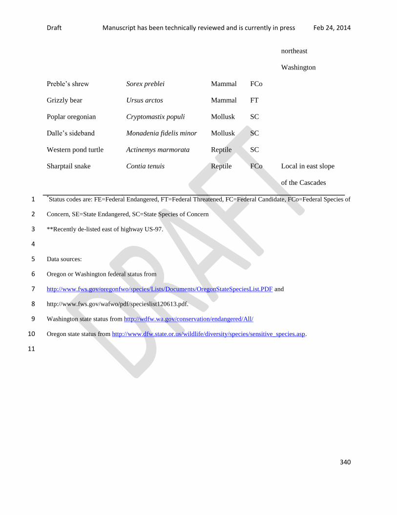
Draft Manuscript has been technically reviewed and is currently in press Feb 24, 2014
340
northeast
Washington
Preble’s shrew Sorex preblei Mammal FCo
Grizzly bear Ursus arctos Mammal FT
Poplar oregonian Cryptomastix populi Mollusk SC
Dalle’s sideband Monadenia fidelis minor Mollusk SC
Western pond turtle Actinemys marmorata Reptile SC
Sharptail snake Contia tenuis Reptile FCo Local in east slope
of the Cascades
*Status codes are: FE=Federal Endangered, FT=Federal Threatened, FC=Federal Candidate, FCo=Federal Species of 1
Concern, SE=State Endangered, SC=State Species of Concern 2
**Recently de-listed east of highway US-97. 3
4
Data sources: 5
Oregon or Washington federal status from 6
http://www.fws.gov/oregonfwo/species/Lists/Documents/OregonStateSpeciesList.PDF and 7
http://www.fws.gov/wafwo/pdf/specieslist120613.pdf. 8
Washington state status from http://wdfw.wa.gov/conservation/endangered/All/ 9
Oregon state status from http://www.dfw.state.or.us/wildlife/diversity/species/sensitive_species.asp. 10
11

Draft Manuscript has been technically reviewed and is currently in press Feb 24, 2014
341
Table C1—Percentage of sampled area in the Blue Mountains ERU by potential vegetation type 1
Potential Vegetation Type Hectares PCT_ERU
ponderosa pine 15,624.56 3.77
WD Douglas-fir/grand fir 40,208.19 9.70
CM Douglas-fir/grand fir 191,632.00 46.22
WD subalpine fir/Engelmann spruce 16,903.80 4.08
CM subalpine fir/Engelmann spruce 33,475.22 8.07
Total 297,843.76 71.83
2
3
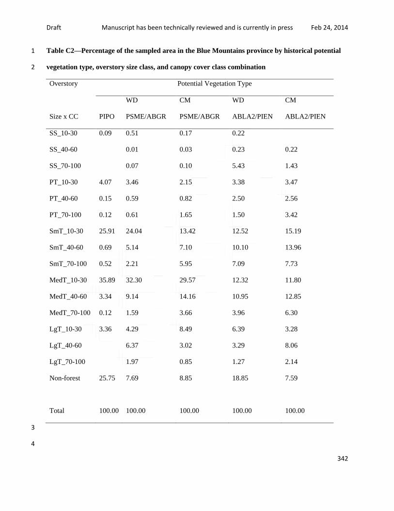
Draft Manuscript has been technically reviewed and is currently in press Feb 24, 2014
342
Table C2—Percentage of the sampled area in the Blue Mountains province by historical potential 1
vegetation type, overstory size class, and canopy cover class combination 2
Overstory Potential Vegetation Type
Size x CC PIPO
WD
PSME/ABGR
CM
PSME/ABGR
WD
ABLA2/PIEN
CM
ABLA2/PIEN
SS_10-30 0.09 0.51 0.17 0.22
SS_40-60 0.01 0.03 0.23 0.22
SS_70-100 0.07 0.10 5.43 1.43
PT_10-30 4.07 3.46 2.15 3.38 3.47
PT_40-60 0.15 0.59 0.82 2.50 2.56
PT_70-100 0.12 0.61 1.65 1.50 3.42
SmT_10-30 25.91 24.04 13.42 12.52 15.19
SmT_40-60 0.69 5.14 7.10 10.10 13.96
SmT_70-100 0.52 2.21 5.95 7.09 7.73
MedT_10-30 35.89 32.30 29.57 12.32 11.80
MedT_40-60 3.34 9.14 14.16 10.95 12.85
MedT_70-100 0.12 1.59 3.66 3.96 6.30
LgT_10-30 3.36 4.29 8.49 6.39 3.28
LgT_40-60 6.37 3.02 3.29 8.06
LgT_70-100 1.97 0.85 1.27 2.14
Non-forest 25.75 7.69 8.85 18.85 7.59
Total 100.00 100.00 100.00 100.00 100.00
3
4

Draft Manuscript has been technically reviewed and is currently in press Feb 24, 2014
343
Table C3—Percentage of the sampled area in the Blue Mountains ERU by historical potential 1
vegetation type, understory size class, and canopy cover class combination 2
Understory Potential Vegetation Type
Size x CC PIPO
WD
PSME/ABGR
CM
PSME/ABGR
WD
ABLA2/PIEN
CM
ABLA2/PIEN
SS_10-30 21.69 18.49 7.25 2.32 6.76
SS_40-60 2.35 6.53 1.55 2.01 2.45
SS_70-90 1.30 0.38 0.24 1.03
PT_10-30 23.45 24.61 26.22 24.94 25.15
PT_40-60 3.96 7.61 10.14 6.84 5.89
PT_70-90 1.20 0.49 1.30 1.56 1.52
SmT_10-30 1.73 8.56 15.47 11.14 17.09
SmT_40-60 0.04 2.14 8.44 2.62 5.50
SmT_70-90 0.47 0.98 0.18 0.69
MedT_10-30 0.21 1.62 0.06 0.09
MedT_40-60 0.05 1.26 0.12
MedT_70-90 0.20
Without any US 19.83 21.85 16.34 29.10 26.24
Non-forest 25.75 7.69 8.85 18.85 7.59
Total 100.00 100.00 100.00 100.00 100.00
3
4
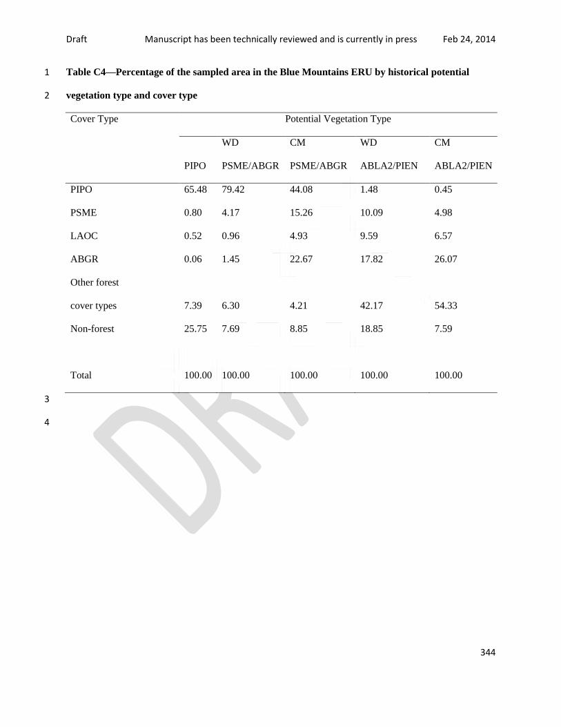
Draft Manuscript has been technically reviewed and is currently in press Feb 24, 2014
344
Table C4—Percentage of the sampled area in the Blue Mountains ERU by historical potential 1
vegetation type and cover type 2
Cover Type Potential Vegetation Type
PIPO
WD
PSME/ABGR
CM
PSME/ABGR
WD
ABLA2/PIEN
CM
ABLA2/PIEN
PIPO 65.48 79.42 44.08 1.48 0.45
PSME 0.80 4.17 15.26 10.09 4.98
LAOC 0.52 0.96 4.93 9.59 6.57
ABGR 0.06 1.45 22.67 17.82 26.07
Other forest
cover types 7.39 6.30 4.21 42.17 54.33
Non-forest 25.75 7.69 8.85 18.85 7.59
Total 100.00 100.00 100.00 100.00 100.00
3
4

Draft Manuscript has been technically reviewed and is currently in press Feb 24, 2014
345
Table C5—Percentage of the sampled area in the Blue Mountains ERU by historical potential 1
vegetation type, cover type, size class, and canopy cover class 2
Cover Potential Vegetation Type
OS Size x CC PIPO
WD
PSME/ABGR
CM
PSME/ABGR
WD
ABLA2/PIEN
CM
ABLA2/PIEN
PIPO
SS_10-30 0.46 0.16
SS_40-60 0.01
SS_70-100 0.04 0.02
PT_10-30 2.05 1.56 1.24 0.53
PT_40-60 0.06 0.42 0.34
PT_70-100 0.12 0.51 0.14 0.09
SmT_10-30 23.71 20.66 8.60 0.17 0.26
SmT_40-60 0.29 3.47 3.00 0.18 0.02
SmT_70-100 1.69 1.25
MedT_10-30 32.56 28.75 17.93 0.51 0.08
MedT_40-60 3.26 8.22 6.56
MedT_70-100 0.12 1.44 0.35
LgT_10-30 3.31 3.91 3.73 0.09
LgT_40-60 6.32 0.66
LgT_70-100 1.94 0.09
PSME
SS_10-30 0.01 0.12
SS_40-60 0.02 0.23
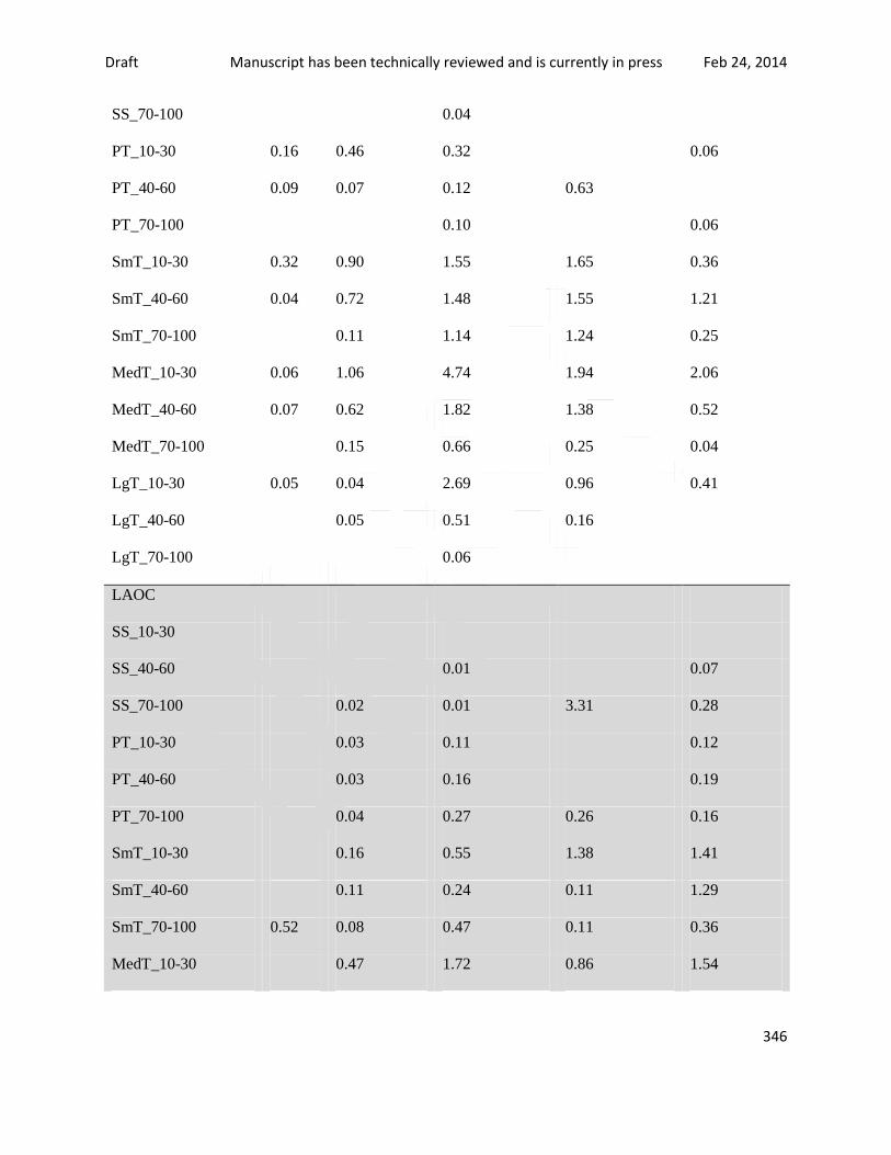
Draft Manuscript has been technically reviewed and is currently in press Feb 24, 2014
346
SS_70-100 0.04
PT_10-30 0.16 0.46 0.32 0.06
PT_40-60 0.09 0.07 0.12 0.63
PT_70-100 0.10 0.06
SmT_10-30 0.32 0.90 1.55 1.65 0.36
SmT_40-60 0.04 0.72 1.48 1.55 1.21
SmT_70-100 0.11 1.14 1.24 0.25
MedT_10-30 0.06 1.06 4.74 1.94 2.06
MedT_40-60 0.07 0.62 1.82 1.38 0.52
MedT_70-100 0.15 0.66 0.25 0.04
LgT_10-30 0.05 0.04 2.69 0.96 0.41
LgT_40-60 0.05 0.51 0.16
LgT_70-100 0.06
LAOC
SS_10-30
SS_40-60 0.01 0.07
SS_70-100 0.02 0.01 3.31 0.28
PT_10-30 0.03 0.11 0.12
PT_40-60 0.03 0.16 0.19
PT_70-100 0.04 0.27 0.26 0.16
SmT_10-30 0.16 0.55 1.38 1.41
SmT_40-60 0.11 0.24 0.11 1.29
SmT_70-100 0.52 0.08 0.47 0.11 0.36
MedT_10-30 0.47 1.72 0.86 1.54

Draft Manuscript has been technically reviewed and is currently in press Feb 24, 2014
347
MedT_40-60 0.01 0.59 2.70 0.59
MedT_70-100 0.24 0.05 0.10
LgT_10-30 0.20 0.80 0.46
LgT_40-60 0.36
LgT_70-100
ABGR
SS_10-30
SS_40-60
SS_70-100 0.08
PT_10-30 0.28 0.25 0.36
PT_40-60 0.02 0.14 0.69
PT_70-100 0.24 0.36 0.07
SmT_10-30 0.03 0.01 2.26 1.77 2.04
SmT_40-60 0.67 2.25 3.03 4.70
SmT_70-100 0.14 2.54 1.51 2.84
MedT_10-30 0.03 0.17 3.82 2.30 2.40
MedT_40-60 0.23 5.12 2.48 4.16
MedT_70-100 2.40 2.02 3.21
LgT_10-30 0.20 1.58 1.27 0.27
LgT_40-60 1.48 2.24 3.93
LgT_70-100 0.03 0.68 0.45 1.35
Other forest cover
types
SS_10-30 0.09 0.05 0.10
Draft Manuscript has been technically reviewed and is currently in press Feb 24, 2014
348
SS_40-60 0.15
SS_70-100 0.03 2.11 1.07
PT_10-30 1.86 1.42 0.21 2.61 2.93
PT_40-60 0.07 0.18 1.72 1.67
PT_70-100 0.06 0.90 0.87 3.05
SmT_10-30 1.85 2.31 0.46 7.56 11.12
SmT_40-60 0.36 0.16 0.12 5.23 6.74
SmT_70-100 0.18 0.55 4.23 4.28
MedT_10-30 3.23 1.86 1.36 6.72 5.72
MedT_40-60 0.06 0.07 4.40 7.58
MedT_70-100 0.01 1.65 2.95
LgT_10-30 0.13 0.28 3.27 2.15
LgT_40-60 0.89 4.14
LgT_70-100 0.02 0.82 0.79
Non-forest 25.75 7.69 8.85 18.85 7.59
Grand Total 100.00 100.00 100.00 100.00 100.00
1
2

Draft Manuscript has been technically reviewed and is currently in press Feb 24, 2014
349
Table C6—Percentage of the sampled area in the Blue Mountains ERU by historical potential 1
vegetation type, cover type, and structural class 2
Cover x Structure Potential Vegetation Type
PIPO
WD
PSME/ABGR
CM
PSME/ABGR
WD
ABLA2/PIEN
CM
ABLA2/PIEN
PIPO
si 21.23 16.59 3.06 0.06
seoc 31.35 27.60 11.95 0.78 0.14
secc 0.04 2.48 1.56 0.18 0.23
ur 3.32 8.72 7.70 0.19 0.08
yfms 9.44 14.51 17.64 0.27
ofms 0.11 5.60 1.40
ofss
3.91 0.78
PSME
si
0.49 0.68 1.11 0.11
seoc 0.29 2.09 2.63 2.72 1.32
secc
0.15 1.81 1.98 0.55
ur 0.44 0.54 3.19 1.68 1.57
yfms 0.07 0.85 6.15 2.32 1.44
ofms
0.03 0.28 0.27
ofss
0.02 0.53
LAOC
si
0.02 0.45 3.85 1.07
seoc
0.13 0.14 0.11 0.27
Draft Manuscript has been technically reviewed and is currently in press Feb 24, 2014
350
secc 0.52 0.13 0.93 1.59 1.51
ur
0.53 1.54 2.94 2.67
yfms
0.15 1.40 0.41 1.05
ofms
0.46 0.68
ofss
0.01
ABGR
si
0.11
0.23
seoc 0.06 0.18 7.20 4.22 4.07
secc
0.50 2.65 3.15 4.74
ur
0.31 3.98 3.82 5.78
yfms
0.23 6.11 3.58 5.89
ofms
0.20 0.59 0.56 1.28
ofss
0.03 2.03 2.48 4.08
Other forest cover
types
si 0.39 0.77 0.13 3.12 4.00
seoc
0.11 0.71 16.18 15.61
secc
0.25 1.14 8.23 7.97
ur
0.49 0.80 6.79 9.77
yfms
0.71 1.28 5.64 10.63
ofms
0.42 2.09
ofss
0.02 1.77 4.27
woodland 7.00 3.99 0.14 0.01
Non-forest

Draft Manuscript has been technically reviewed and is currently in press Feb 24, 2014
351
herbland 15.62 3.27 7.45 13.74 4.56
shrubland 9.80 4.16 0.79 1.39 1.15
non-forest/non-range 0.34 0.27 0.61 3.73 1.89
Grand Total 100.00 100.00 100.00 100.00 100.00
1

Draft Manuscript has been technically reviewed and is currently in press Feb 24, 2014
352
Cover 1
2
3
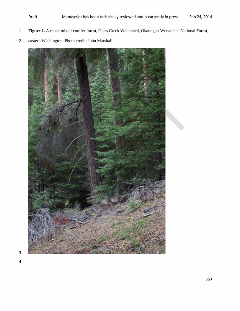
Draft Manuscript has been technically reviewed and is currently in press Feb 24, 2014
353
Figure 1. A moist mixed-conifer forest, Glass Creek Watershed, Okanogan-Wenatchee National Forest, 1
eastern Washington. Photo credit: John Marshall. 2
3
4

Draft Manuscript has been technically reviewed and is currently in press Feb 24, 2014
354
Figure 2. A mixed-conifer landscape, Middle Fork of Gold Creek, Okanogan-Wenatchee National Forest, 1
eastern Washington. Photo credit: John Marshall. 2
3
4
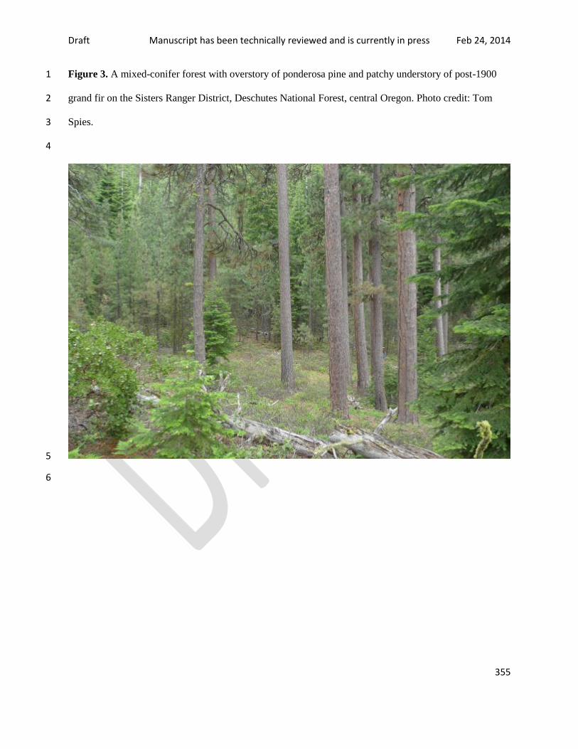
Draft Manuscript has been technically reviewed and is currently in press Feb 24, 2014
355
Figure 3. A mixed-conifer forest with overstory of ponderosa pine and patchy understory of post-1900 1
grand fir on the Sisters Ranger District, Deschutes National Forest, central Oregon. Photo credit: Tom 2
Spies. 3
4
5
6
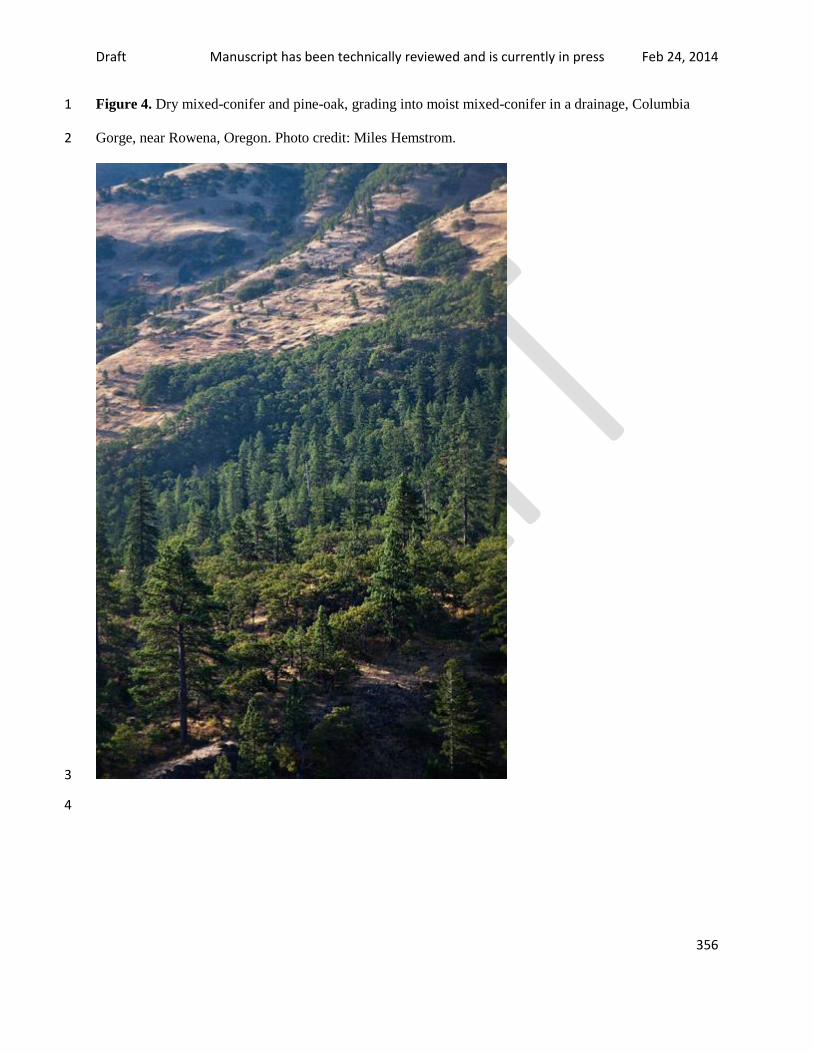
Draft Manuscript has been technically reviewed and is currently in press Feb 24, 2014
356
Figure 4. Dry mixed-conifer and pine-oak, grading into moist mixed-conifer in a drainage, Columbia 1
Gorge, near Rowena, Oregon. Photo credit: Miles Hemstrom. 2
3
4
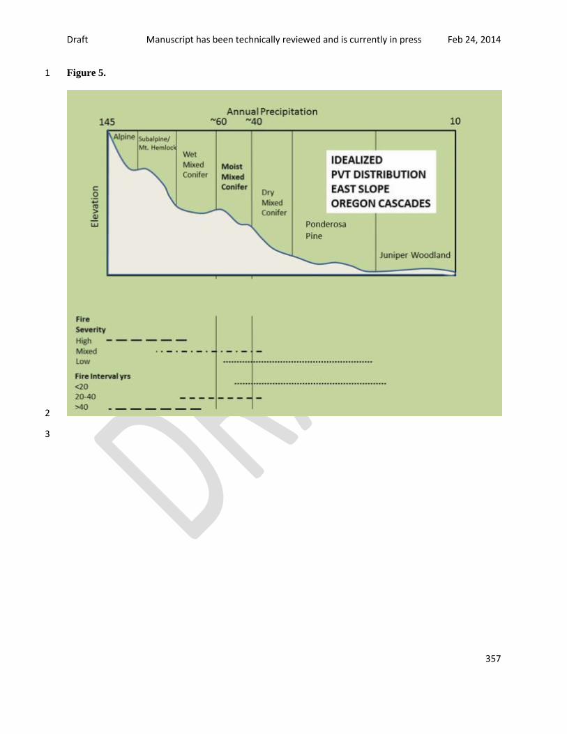
Draft Manuscript has been technically reviewed and is currently in press Feb 24, 2014
357
Figure 5. 1
2
3
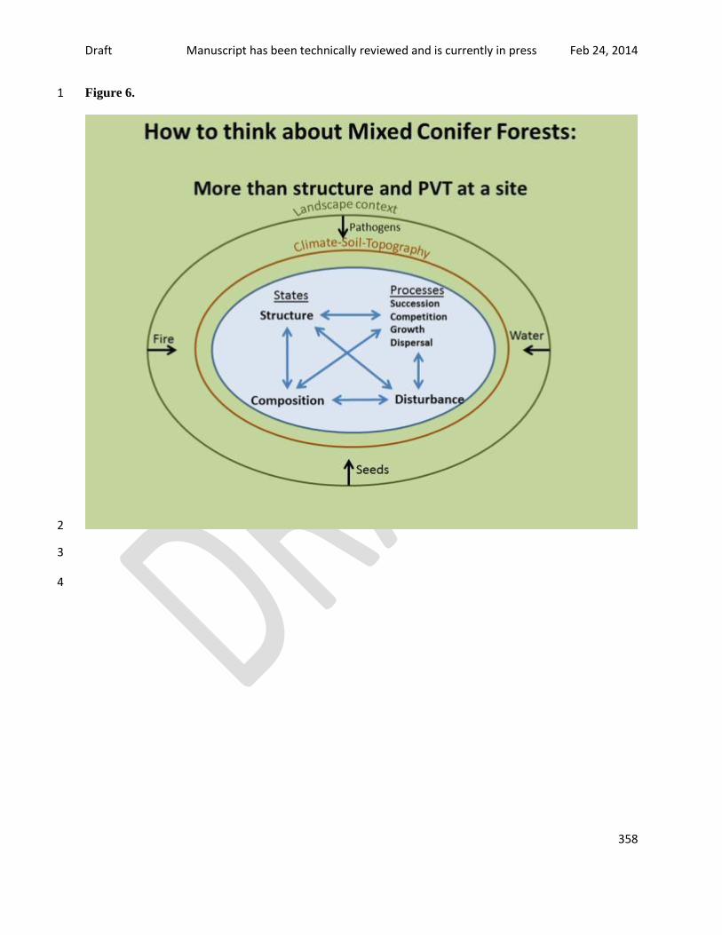
Draft Manuscript has been technically reviewed and is currently in press Feb 24, 2014
358
Figure 6. 1
2
3
4
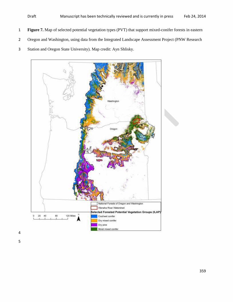
Draft Manuscript has been technically reviewed and is currently in press Feb 24, 2014
359
Figure 7. Map of selected potential vegetation types (PVT) that support mixed-conifer forests in eastern 1
Oregon and Washington, using data from the Integrated Landscape Assessment Project (PNW Research 2
Station and Oregon State University). Map credit: Ayn Shlisky. 3
4
5

Draft Manuscript has been technically reviewed and is currently in press Feb 24, 2014
360
Figure 8. 1
2
3
4
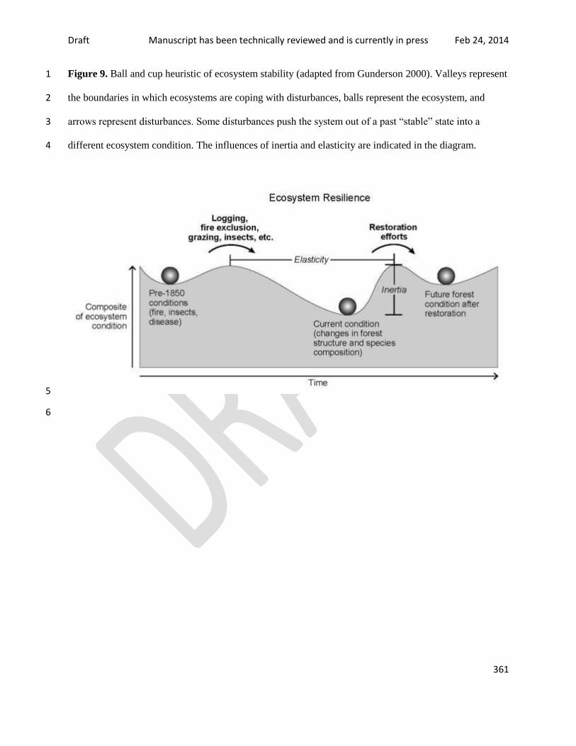
Draft Manuscript has been technically reviewed and is currently in press Feb 24, 2014
361
Figure 9. Ball and cup heuristic of ecosystem stability (adapted from Gunderson 2000). Valleys represent 1
the boundaries in which ecosystems are coping with disturbances, balls represent the ecosystem, and 2
arrows represent disturbances. Some disturbances push the system out of a past “stable” state into a 3
different ecosystem condition. The influences of inertia and elasticity are indicated in the diagram. 4
5
6

Draft Manuscript has been technically reviewed and is currently in press Feb 24, 2014
362
Figure 10. The Mission Peak area on the Okanogan-Wenatchee National Forest; a comparison between 1
1934 and 2010 of forest density and structure. Photo credit: John Marshall. 2
3
4

Draft Manuscript has been technically reviewed and is currently in press Feb 24, 2014
363
Figure 11. At the regional scale, the moisture gradient is structured by large-scale topographic features, 1
such as the Cascade Mountains, and a prevailing south-southwest storm track. 2
3
4
5
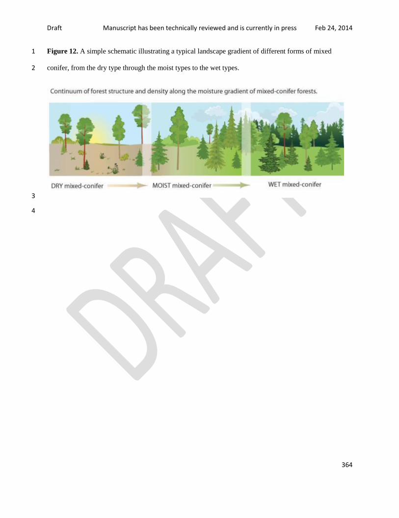
Draft Manuscript has been technically reviewed and is currently in press Feb 24, 2014
364
Figure 12. A simple schematic illustrating a typical landscape gradient of different forms of mixed 1
conifer, from the dry type through the moist types to the wet types. 2
3
4

Draft Manuscript has been technically reviewed and is currently in press Feb 24, 2014
365
Figure 13. A common gradient of grasslands/shrublands to dry forests and moist forests. Blue Mountains 1
near Pendleton, Oregon. Photo credit: Miles Hemstrom. 2
3
4
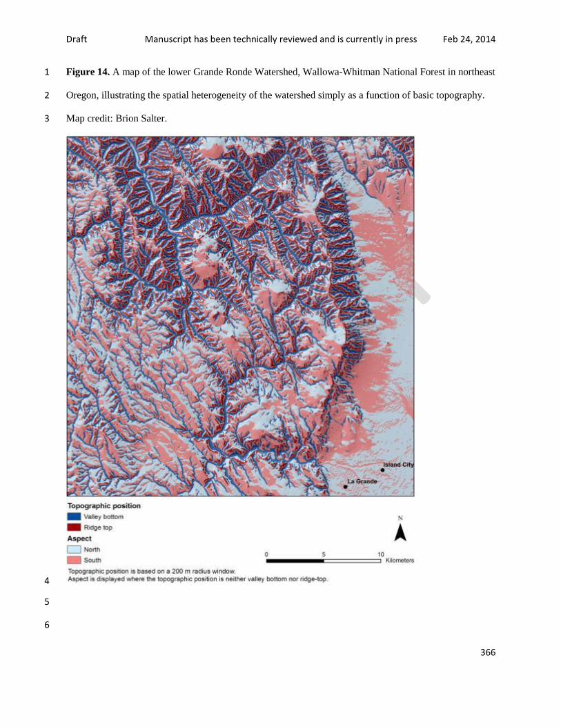
Draft Manuscript has been technically reviewed and is currently in press Feb 24, 2014
366
Figure 14. A map of the lower Grande Ronde Watershed, Wallowa-Whitman National Forest in northeast 1
Oregon, illustrating the spatial heterogeneity of the watershed simply as a function of basic topography. 2
Map credit: Brion Salter. 3
4
5
6
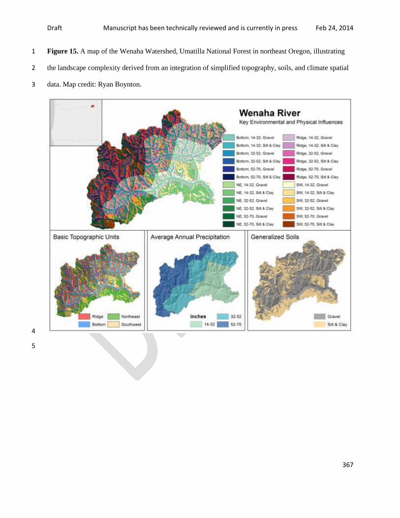
Draft Manuscript has been technically reviewed and is currently in press Feb 24, 2014
367
Figure 15. A map of the Wenaha Watershed, Umatilla National Forest in northeast Oregon, illustrating 1
the landscape complexity derived from an integration of simplified topography, soils, and climate spatial 2
data. Map credit: Ryan Boynton. 3
4
5
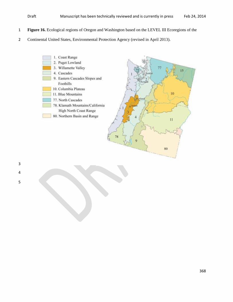
Draft Manuscript has been technically reviewed and is currently in press Feb 24, 2014
368
Figure 16. Ecological regions of Oregon and Washington based on the LEVEL III Ecoregions of the 1
Continental United States, Environmental Protection Agency (revised in April 2013). 2
3
4
5
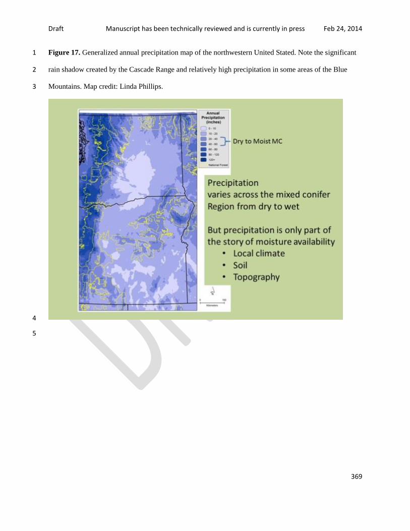
Draft Manuscript has been technically reviewed and is currently in press Feb 24, 2014
369
Figure 17. Generalized annual precipitation map of the northwestern United Stated. Note the significant 1
rain shadow created by the Cascade Range and relatively high precipitation in some areas of the Blue 2
Mountains. Map credit: Linda Phillips. 3
4
5

Draft Manuscript has been technically reviewed and is currently in press Feb 24, 2014
370
Figure 18. Conceptual model of vegetation states and transitions associated with fire severity. Under low- 1
to mixed-severity fire regimes, moist mixed-conifer forest landscapes were dominated by patches 2
characterized by old trees and relatively open understories or old trees in a mosaic of open and dense 3
understory patches (bold boxes in upper right). Forest structure and composition shifted among various 4
structurally diverse stages (boxes in upper unstippled area) depending on ecoregion, fine-scale 5
environmental variation, and amount of high-severity fire. Under fire exclusion and even-age 6
management, forest structure and disturbance regimes have shifted potential forest stages and pathways 7
into the lower region of the diagram (stippled area) where the amount of dense old forest, high-severity 8
fire, and uniform young forest is much greater than it would have been under the pre-Euro-American fire 9
regime. Some old, dense multi-strata forest would have existed under the pre-Euroamerican period but it 10
probably was a small portion of the moist mixed-conifer type across the region. Graphic credit: Tom 11
Spies. 12
13
14

Draft Manuscript has been technically reviewed and is currently in press Feb 24, 2014
371
Figure 19. Historical versus current tree density in dry and moist mixed-conifer forest summarized from 1
five study areas. Methods used to calculate density vary by reference period and study region, and 2
diameter thresholds for tree density vary slightly among regions (10-15 cm). See the notes section in table 3
5 for citations and detailed information on how density was estimated in each region and time period. 4
5
6

Draft Manuscript has been technically reviewed and is currently in press Feb 24, 2014
372
Figure 20. Profiles of predominant forest types, derived from potential vegetation types of Simpson, 1
across an east-west transect for four locations in eastern Oregon and Washington. Topography is 2
exaggerated to show topographic effects. Graphic credit: Keith Olsen. 3
4
5

Draft Manuscript has been technically reviewed and is currently in press Feb 24, 2014
373
Figure 21. At the localized scale, mountainous terrain creates localized gradients in soil moisture, driven 1
principally by differences in exposure to sunlight and wind (e.g., dry windy south-facing aspects versus 2
cool moist north-facing hillslopes). 3
4
5
6

Draft Manuscript has been technically reviewed and is currently in press Feb 24, 2014
374
Figure 22. A sample of seven historical (ca. 1900) maps of combined cover type and structural class 1
conditions from subwatersheds of the eastern Washington Cascades. Gray tones indicate unique cover 2
type-structural class combinations. Note the highly variable patch sizes, with many small and fewer large 3
patches. Despite their fewer numbers, the large patches actually make up the majority area of each 4
subwatershed (adapted from Perry et al. 2011). 5
6
7
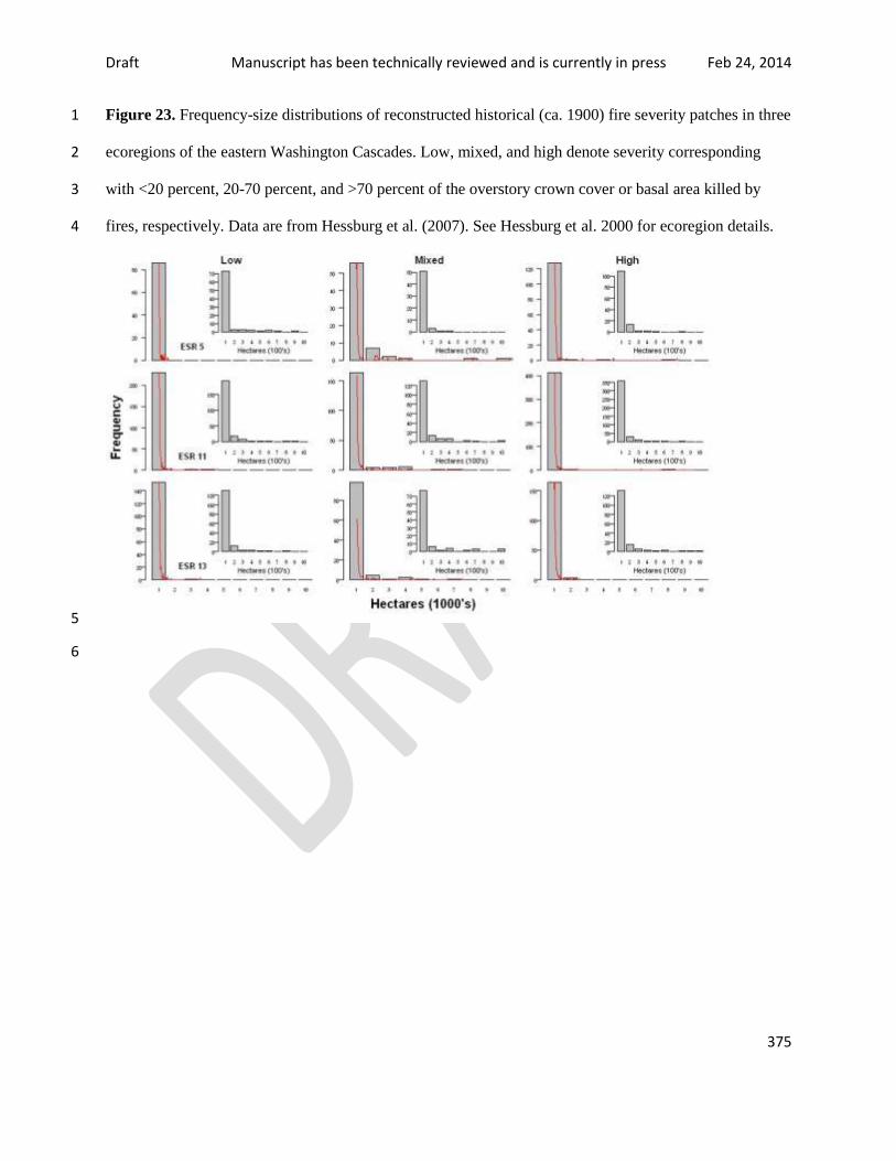
Draft Manuscript has been technically reviewed and is currently in press Feb 24, 2014
375
Figure 23. Frequency-size distributions of reconstructed historical (ca. 1900) fire severity patches in three 1
ecoregions of the eastern Washington Cascades. Low, mixed, and high denote severity corresponding 2
with <20 percent, 20-70 percent, and >70 percent of the overstory crown cover or basal area killed by 3
fires, respectively. Data are from Hessburg et al. (2007). See Hessburg et al. 2000 for ecoregion details. 4
5
6
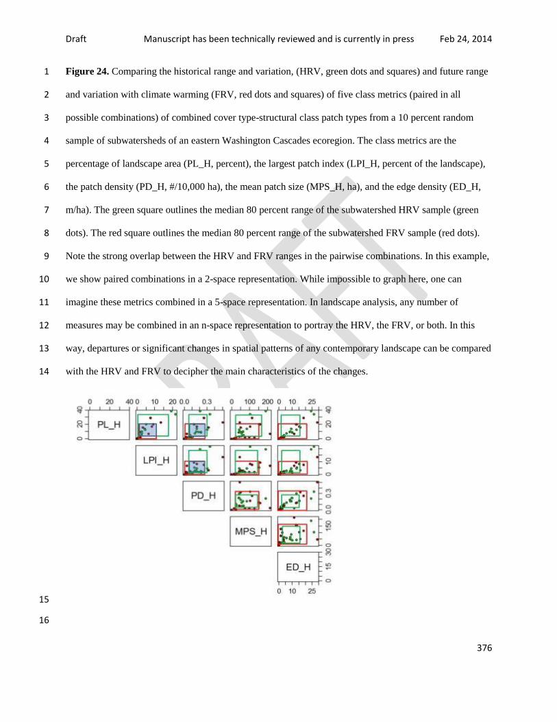
Draft Manuscript has been technically reviewed and is currently in press Feb 24, 2014
376
Figure 24. Comparing the historical range and variation, (HRV, green dots and squares) and future range 1
and variation with climate warming (FRV, red dots and squares) of five class metrics (paired in all 2
possible combinations) of combined cover type-structural class patch types from a 10 percent random 3
sample of subwatersheds of an eastern Washington Cascades ecoregion. The class metrics are the 4
percentage of landscape area (PL_H, percent), the largest patch index (LPI_H, percent of the landscape), 5
the patch density (PD_H, #/10,000 ha), the mean patch size (MPS_H, ha), and the edge density (ED_H, 6
m/ha). The green square outlines the median 80 percent range of the subwatershed HRV sample (green 7
dots). The red square outlines the median 80 percent range of the subwatershed FRV sample (red dots). 8
Note the strong overlap between the HRV and FRV ranges in the pairwise combinations. In this example, 9
we show paired combinations in a 2-space representation. While impossible to graph here, one can 10
imagine these metrics combined in a 5-space representation. In landscape analysis, any number of 11
measures may be combined in an n-space representation to portray the HRV, the FRV, or both. In this 12
way, departures or significant changes in spatial patterns of any contemporary landscape can be compared 13
with the HRV and FRV to decipher the main characteristics of the changes. 14
15
16

Draft Manuscript has been technically reviewed and is currently in press Feb 24, 2014
377
Figure 25. Ecological subregions of the interior Columbia River basin (Hessburg et al. 2000a). Names 1
corresponding with ESR numbers are of the form: [ESR number = Bailey’s (Bailey et al. 1994) ecoregion - 2
Dominant Precipitation class(es) - Dominant Temperature class(es) - Dominant Potential Vegetation Group(s) - 3
Dominant Solar Radiation class(es)] 1 = M330 - Wet - Warm - MF - Mod solar; 2 = M333 - Moist - Warm - MF/DF 4
- Low solar; 3 = M333 - Moist - Cold - MF - Low solar; 4 = M242C - Wet - Warm - MFCF – Low solar; 5 = 5
M242C - Moist - Warm - MF/CF - Mod solar; 6 = M242C - Wet - Cold - CF - Mod/Low solar; 7 = 342I - Dry - 6
Warm - DS - Mod solar; 8 = M333A - Dry - Warm/Hot - DG - Mod solar; 9 = 300 - Moist/Dry - Warm - DS/CS - 7
High solar; 10 = 342I – Dry - Hot - DS/DG - Mod solar; 11 = 200/300 - Dry/Moist - Warm - MF/DF - Mod solar; 12 8
= M330 - Moist - Warm - DF - Mod solar; 13 = 200/300 - Moist - Warm/Cold - MF - Mod solar; 14 = M333A - 9
Moist - Warm/Cold - MF - Mod solar; 15 = M332 - Moist/Wet - Cold - CF/DF - Mod/High solar; 16 = 330 - Moist - 10
Hot - DG - Mod solar; 17 = M333C - Wet - Cold - MF/CF - Low solar; 18 = M330 - Moist - Warm - DF/DG - Mod 11
solar; 19 = M330 - Wet - Cold - MF/CF - Mod solar; 20 = M330 - Moist - Cold/Warm – MF - Mod solar; 21 = 331A 12
- Moist - Warm - DG - Low solar; 22 = 200 - Moist/Dry - Warm - DF - Very high/High solar; 23 = M333D - Wet - 13
Warm/Cold - MF - Low solar; 24 = M332 - Moist/Wet - Cold - CF/DF/MF - High solar; 25 = M332 - Moist - Cold - 14
DF/CF - High solar; 26 = M332 - Moist/Dry - Cold - CF - High/Mod solar; 27 = 300 - Dry - Warm - CS/DF - High 15
solar; 28 = 200 – Moist - Warm - DF/DG - High solar; 29 = M332 - Dry - Cold - DS/CS - High solar; 30 = 300 - 16
Moist - Warm - DG/DF - Mod solar; 31 = 300 - Moist - Warm - DF/DG - Mod solar; 32 = M332F - Moist - 17
Cold/Frigid - CF - High/Very high solar; 34 = M332 - Moist - Warm/ Cold - DF/CS - High solar; 35 = M332 - Moist 18
- Cold - CF/DG - High/Very high solar; 36 = M332 - Dry - Cold/Warm - DS/CS – High solar; 37 = M332B - Wet - 19
Cold - RK/CF - Mod solar; 38 = M332 - Moist - Cold - CF/DF/DG - Mod solar; 39 = M332B - Moist - Warm/Cold - 20
DF/CF/DG - Mod solar; 40 = 200 - Moist - Warm/Cold - DF - High/Very high solar; 41 = M242C - Moist - Warm - 21
MF/DF/CF - High solar; 42 = 300 - Dry - Warm - DS/CS - Very high solar; 43 = M331D - Moist - Cold - 22
CF/DF/WD - Very high solar; 44 = 342 - Dry/Moist - Warm - DS/CS - Very high solar; 45 = 342H - Dry - 23
Warm/Hot - DS/CS - High solar; 46 = M242C – Moist - Warm - DF - High solar; 47 = 342C - Dry - Hot - DS/RS - 24
High solar; 48 = 342 - Dry - Warm - DS - High solar; 50 = M331 - Moist/Wet - Cold/Frigid - CF - High solar; 51 = 25
300 - Moist/Dry - Warm - DS/WD - High solar; 52 = M331 - Moist - Cold - CF/WD – High solar; 53 = M242C - 26
Moist - Cold - CF - Mod solar; 54 = M332 - Moist - Warm - MF/DF - Mod solar; 55 = M331D - Moist – Cold - WD 27
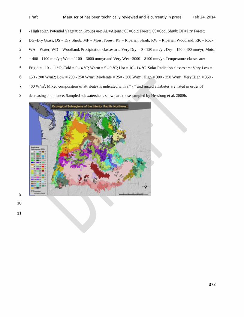
Draft Manuscript has been technically reviewed and is currently in press Feb 24, 2014
378
- High solar. Potential Vegetation Groups are: AL=Alpine; CF=Cold Forest; CS=Cool Shrub; DF=Dry Forest; 1
DG=Dry Grass; DS = Dry Shrub; MF = Moist Forest; RS = Riparian Shrub; RW = Riparian Woodland; RK = Rock; 2
WA = Water; WD = Woodland. Precipitation classes are: Very Dry = 0 - 150 mm/yr; Dry = 150 - 400 mm/yr; Moist 3
= 400 - 1100 mm/yr; Wet = 1100 – 3000 mm/yr and Very Wet =3000 – 8100 mm/yr. Temperature classes are: 4
Frigid = –10 - –1 °C; Cold = 0 - 4 °C; Warm = 5 - 9 °C; Hot = 10 - 14 °C. Solar Radiation classes are: Very Low = 5
150 - 200 W/m2; Low = 200 - 250 W/m2; Moderate = 250 - 300 W/m
2; High = 300 - 350 W/m
2; Very High = 350 - 6
400 W/m2. Mixed composition of attributes is indicated with a “ / ” and mixed attributes are listed in order of 7
decreasing abundance. Sampled subwatersheds shown are those sampled by Hessburg et al. 2000b. 8
9
10
11

Draft Manuscript has been technically reviewed and is currently in press Feb 24, 2014
379
Figure 26. An example of a low-severity prescribed fire. These fires are characterized by minimal short-1
term ecosystem effects. The result of a low-severity fire is fuel reduction and topkill of understory 2
vegetation. Photo credit: Roger Ottmar. 3
4
5
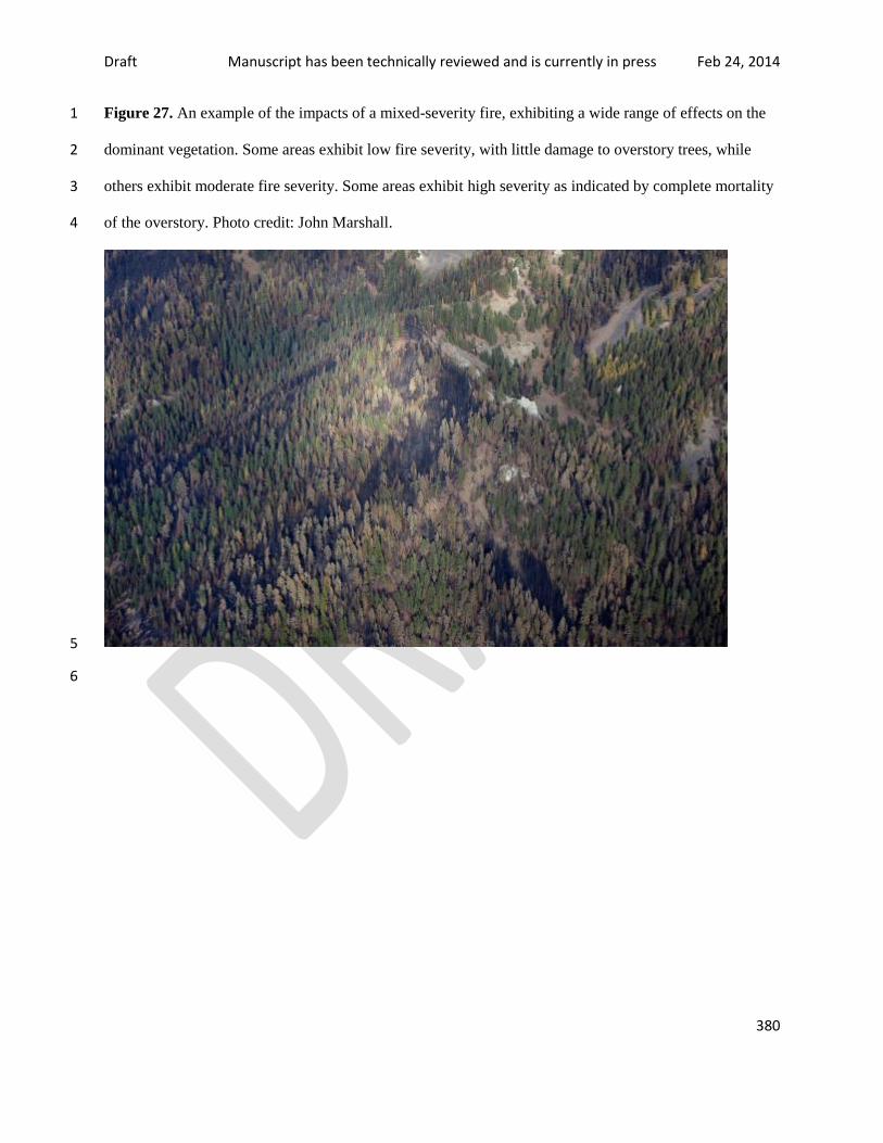
Draft Manuscript has been technically reviewed and is currently in press Feb 24, 2014
380
Figure 27. An example of the impacts of a mixed-severity fire, exhibiting a wide range of effects on the 1
dominant vegetation. Some areas exhibit low fire severity, with little damage to overstory trees, while 2
others exhibit moderate fire severity. Some areas exhibit high severity as indicated by complete mortality 3
of the overstory. Photo credit: John Marshall. 4
5
6

Draft Manuscript has been technically reviewed and is currently in press Feb 24, 2014
381
Figure 28. An example of a high-severity fire, characterized by high levels of tree mortality, significant 1
fuel consumption, and often extensive soil heating. Photo credit: John Marshall. 2
3
4
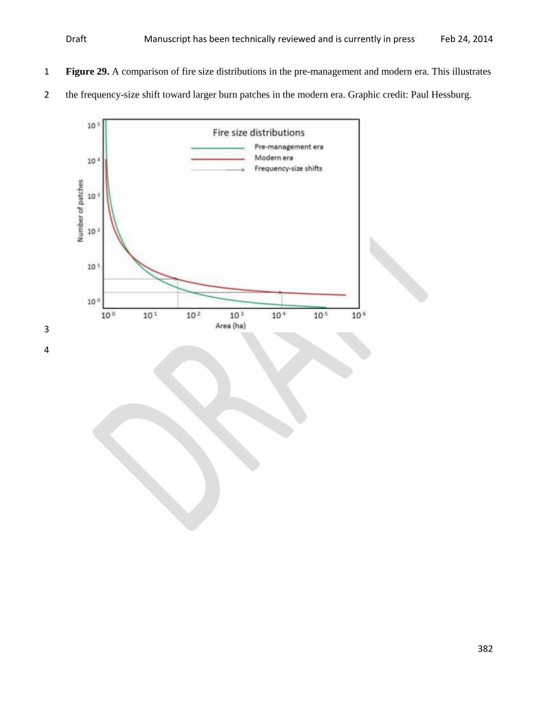
Draft Manuscript has been technically reviewed and is currently in press Feb 24, 2014
382
Figure 29. A comparison of fire size distributions in the pre-management and modern era. This illustrates 1
the frequency-size shift toward larger burn patches in the modern era. Graphic credit: Paul Hessburg. 2
3
4

Draft Manuscript has been technically reviewed and is currently in press Feb 24, 2014
383
Figure 30. Douglas-fir tussock moth larvae. Photo credit: Lia Spiegel. 1
2
3
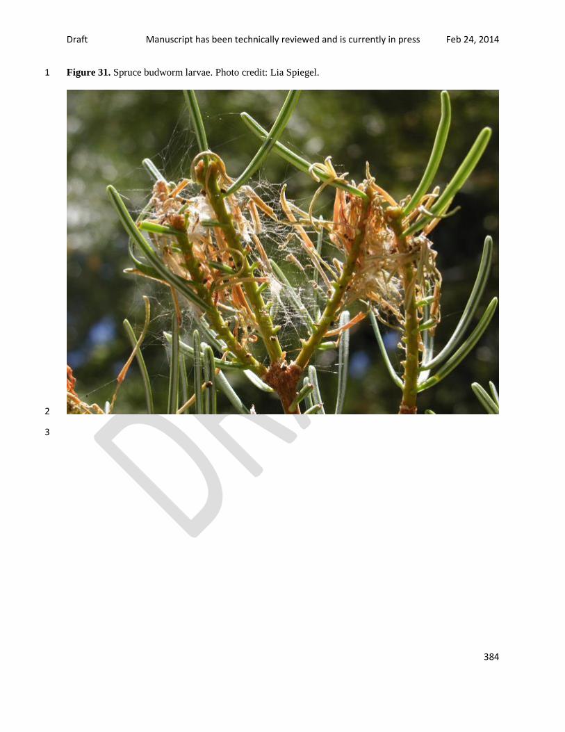
Draft Manuscript has been technically reviewed and is currently in press Feb 24, 2014
384
Figure 31. Spruce budworm larvae. Photo credit: Lia Spiegel. 1
2
3

Draft Manuscript has been technically reviewed and is currently in press Feb 24, 2014
385
Figure 32. Tree mortality attributed to mountain pine beetle. Photo credit: Chris Fettig. 1
2
3

Draft Manuscript has been technically reviewed and is currently in press Feb 24, 2014
386
Figure 33. Wildlife habitat is represented at different scales. Individual animals are connected to key 1
features of their environment over a confined spatial domain, small groups of a species interact regularly 2
over a larger area, and populations of a species are distributed across large geographic areas. This multi-3
scalar view illustrates the importance of considering habitat requirements of a species at different spatial 4
scales. Graphic credit: Keith Routman. 5
6
7

Draft Manuscript has been technically reviewed and is currently in press Feb 24, 2014
387
Figure 34. At a regional scale, habitat for large carnivores is more or less permeable to movement, 1
depending on various vegetation and topographic conditions. This information is an important 2
consideration when planning treatments for forests at a landscape scale. Graphic credit: Peter Singleton. 3
4
5

Draft Manuscript has been technically reviewed and is currently in press Feb 24, 2014
388
Figure 35. Post-fire and other recently disturbed forest sites provide productive habitat for many wildlife 1
species. This recently burned area on the Okanogan-Wenatchee National Forest has shrub and herbaceous 2
vegetation that provides habitat features generally not found in more mature forests. Photo credit: Peter 3
Singleton. 4
5
6
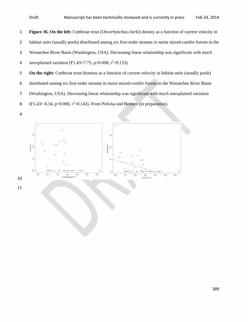
Draft Manuscript has been technically reviewed and is currently in press Feb 24, 2014
389
Figure 36. On the left: Cutthroat trout (Oncorhynchus clarki) density as a function of current velocity in 1
habitat units (usually pools) distributed among six first-order streams in moist mixed-conifer forests in the 2
Wenatchee River Basin (Washington, USA). Decreasing linear relationship was significant with much 3
unexplained variation (F1,43=7.75, p=0.008, r2=0.133). 4
On the right: Cutthroat trout biomass as a function of current velocity in habitat units (usually pools) 5
distributed among six first-order streams in moist mixed-conifer forests in the Wenatchee River Basin 6
(Washington, USA). Decreasing linear relationship was significant with much unexplained variation 7
(F1,43= 8.34, p=0.006, r2=0.143). From Polivka and Bennett (in preparation). 8
9
10
11

Draft Manuscript has been technically reviewed and is currently in press Feb 24, 2014
390
Figure 37. Timber harvest and road development over the last 100 years have had an impact on the 1
spatial configuration of mixed-conifer forests in eastern Oregon and Washington. The image on the left 2
shows a portion of the Umatilla National Forest without stand management, fragmentation with land 3
ownership, and roads. The image on the right shows the effects of land ownership, roads, and harvest 4
units on forest pattern. Graphics from Google Earth. 5
6
7
8
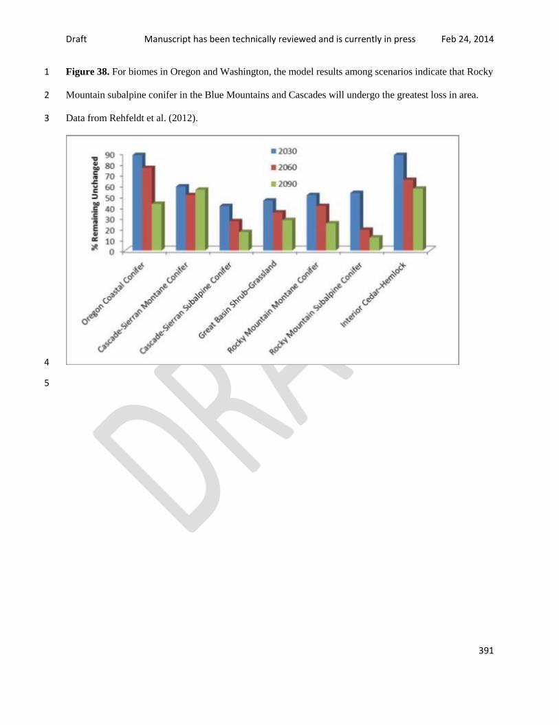
Draft Manuscript has been technically reviewed and is currently in press Feb 24, 2014
391
Figure 38. For biomes in Oregon and Washington, the model results among scenarios indicate that Rocky 1
Mountain subalpine conifer in the Blue Mountains and Cascades will undergo the greatest loss in area. 2
Data from Rehfeldt et al. (2012). 3
4
5

Draft Manuscript has been technically reviewed and is currently in press Feb 24, 2014
392
Figure 39. Showing historical snowpack decline in the Pacific Northwest region 1950-2000 (Mote 2009). 1
2
3

Draft Manuscript has been technically reviewed and is currently in press Feb 24, 2014
393
Figure 40. Projected changes in minimum temperature throughout the Pacific Northwest. 1
2
3
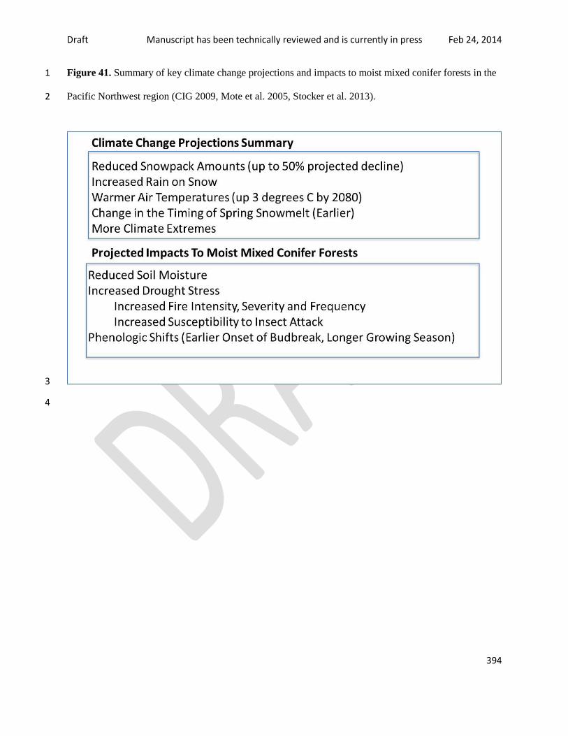
Draft Manuscript has been technically reviewed and is currently in press Feb 24, 2014
394
Figure 41. Summary of key climate change projections and impacts to moist mixed conifer forests in the 1
Pacific Northwest region (CIG 2009, Mote et al. 2005, Stocker et al. 2013). 2
3
4
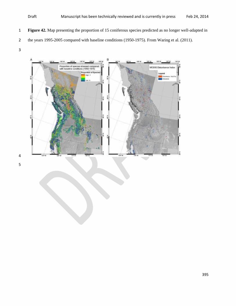
Draft Manuscript has been technically reviewed and is currently in press Feb 24, 2014
395
Figure 42. Map presenting the proportion of 15 coniferous species predicted as no longer well-adapted in 1
the years 1995-2005 compared with baseline conditions (1950-1975). From Waring et al. (2011). 2
3
4
5
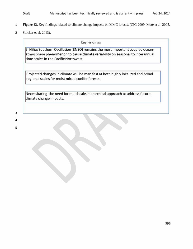
Draft Manuscript has been technically reviewed and is currently in press Feb 24, 2014
396
Figure 43. Key findings related to climate change impacts on MMC forests. (CIG 2009, Mote et al. 2005, 1
Stocker et al. 2013). 2
3
4
5

Draft Manuscript has been technically reviewed and is currently in press Feb 24, 2014
397
Figure 44. Comparison of an example watershed from the early (ca. 1900, historical) and late (1990s, 1
current) 20th century. Note how spatial patterns of fuel loading, crown fire potential, and flame length 2
closely track forest structural conditions: in other words, process followed pattern. Maps are of the 3
Peavine Creek drainage, a dry forest subwatershed of Lower Grande Ronde subbasin in the Blue 4
Mountains Province displaying historical and current structural classes (A and B), fuel loading (C and D), 5
crown fire potential (E and F), and flame length during wildfire (G and H). Fuel loading classes are: very 6
low <22.5 Mg/ha; low = 22.5-44.9 mg/ha; moderate = 45-56.1 Mg/ha; high = 56.2-67.3 Mg/ha; very high 7
>67.3 Mg/ha. Crown fire potential classes were a relativized index. Flame length classes were: very low 8
<0.6 m; low = 0.7-1.2m; moderate = 1.3-1.8 m; high = 1.9-2.4 m; very high = 2.5-3.4 m; severe >3.4 m 9
(Hessburg and Agee 2003, Hessburg et al. 2005). 10
11
12

Draft Manuscript has been technically reviewed and is currently in press Feb 24, 2014
398
Figure 45. Fine-scale structural diversity associated with dwarf mistletoe clumps and other tree defects 1
provide important habitat components for many wildlife species. This Douglas-fir tree is severely infested 2
with dwarf mistletoe. 3
4
5

Draft Manuscript has been technically reviewed and is currently in press Feb 24, 2014
399
Figure 46. Conceptual illustration of the extent to which current ecosystem conditions (CC) in a place 1
differ from the historical range of variability (HRV) in conditions and from projected future conditions 2
(FC). Graphic credit: Andrew Hansen. 3
4
5
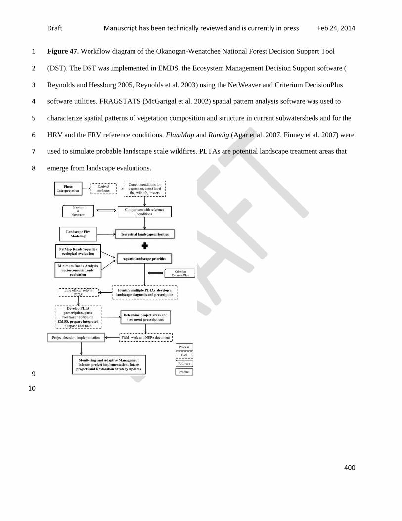
Draft Manuscript has been technically reviewed and is currently in press Feb 24, 2014
400
Figure 47. Workflow diagram of the Okanogan-Wenatchee National Forest Decision Support Tool 1
(DST). The DST was implemented in EMDS, the Ecosystem Management Decision Support software ( 2
Reynolds and Hessburg 2005, Reynolds et al. 2003) using the NetWeaver and Criterium DecisionPlus 3
software utilities. FRAGSTATS (McGarigal et al. 2002) spatial pattern analysis software was used to 4
characterize spatial patterns of vegetation composition and structure in current subwatersheds and for the 5
HRV and the FRV reference conditions. FlamMap and Randig (Agar et al. 2007, Finney et al. 2007) were 6
used to simulate probable landscape scale wildfires. PLTAs are potential landscape treatment areas that 7
emerge from landscape evaluations. 8
9
10

Draft Manuscript has been technically reviewed and is currently in press Feb 24, 2014
401
Figure 48. Example of a 32-ha (80-acre) ponderosa pine and Douglas-fir treatment from the Okanagan-1
Wenatchee National Forest. The treatment was designed to restore a pattern of individual trees, clumps, 2
and openings consistent with pre-fire exclusion conditions. The prescription included specific guidelines 3
for retentions of clumps of different sizes, as well as openings (Churchill et al. 2013). Large openings 4
were flagged out during layout and were often sinuous in shape. Smaller openings occurred as a result of 5
leaving clumps. Large skips (0.2 to 1.2 ha [0.5 to 3 acres]) were included to protect a riparian buffer in the 6
middle of the unit and other biological hotspots such as large Douglas-fir with dwarf mistletoe, 7
concentrations of downed logs, and multistory patches. Note how the unit boundaries were used to create 8
an additional "finger" skip that extends into the stand. A 2-ha (5-acre) square area is shown to indicate the 9
approximate size of an area that should contain a skip or large clump to break up siting distances. For 10
more details on this approach see: 11
http://www.cfc.umt.edu/forestecology/files/ICO_Manager_Guide_V2.pdf Graphic credit: Derek 12
Churchill. 13
14
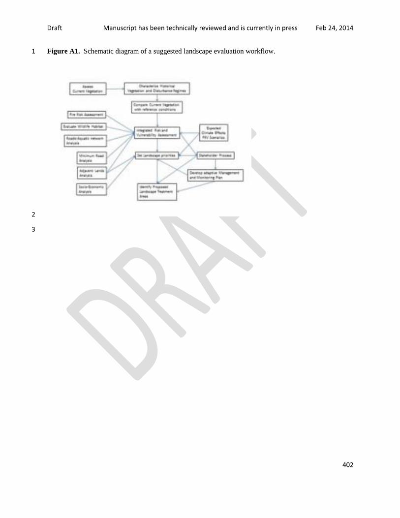
Draft Manuscript has been technically reviewed and is currently in press Feb 24, 2014
402
Figure A1. Schematic diagram of a suggested landscape evaluation workflow. 1
2
3

Draft Manuscript has been technically reviewed and is currently in press Feb 24, 2014
403
Figure C1. Subwatersheds sampled in the Blue Mountains ecological reporting unit (ERU) during 1
Interior Columbia Basin Ecosystem Management Project (Hann et al. 1997; Hessburg et al. 1999b, 2
2000c). The black outline delimits the sampled Blue Mountains area; the white lines delineated the 3
reconstructed subwatersheds. 4
5
6
7