Dr. Nopporn Patcharaprakiti Rajamangala University of ... 2014/Day 1_Power Quality/Modeling...
70
Modeling and Control of Photovoltaic Grid Connected Inverter Based on Nonlinear System Identification for Power Quality Analysis Dr. Nopporn Patcharaprakiti Rajamangala University of Technology Lanna Chiangrai 19 May 2014 PQSynergy 2014 19 May 2014
Transcript of Dr. Nopporn Patcharaprakiti Rajamangala University of ... 2014/Day 1_Power Quality/Modeling...
Modeling and Control of Photovoltaic Grid Connected Inverter Based on Nonlinear System
Identification for Power Quality Analysis
Dr. Nopporn PatcharaprakitiRajamangala University of Technology Lanna Chiangrai
19 May 2014
PQSynergy 2014 19 May 2014

TOPIC
INTRODUCTION
MATHEMATICAL MODELING NONLINEAR SYSTEM IDENTIFICATION
CASE STUDY WITH PV INVERTER POWER QUALITY ANALYSIS MODELING APPLICATION CONCLUSION
PQSynergy 16 May 2014
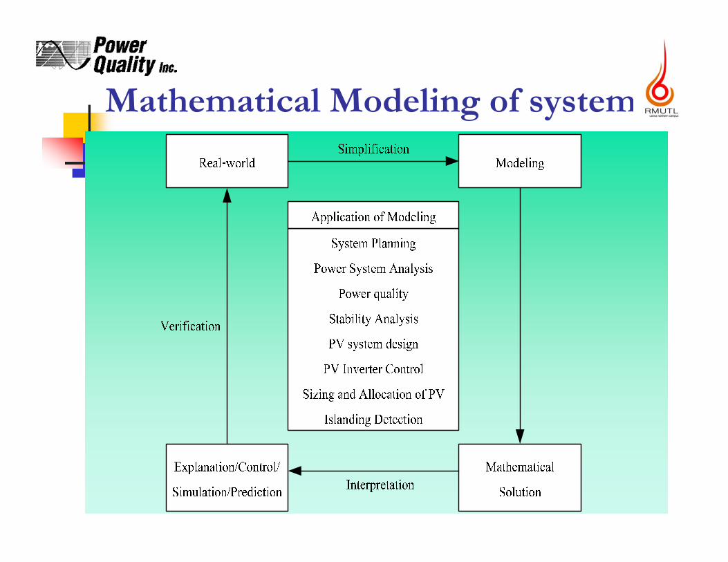
Mathematical Modeling of system
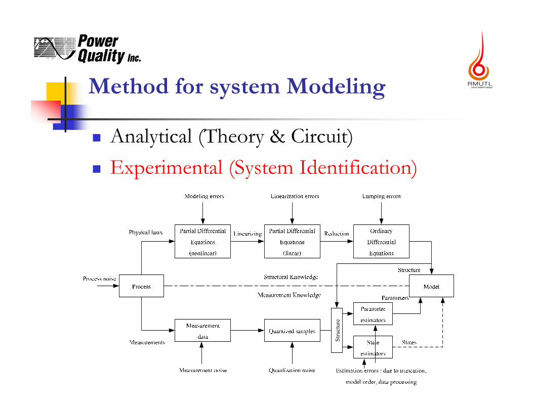
Method for system Modeling
Analytical (Theory & Circuit) Experimental (System Identification)
Stru
ctur
e
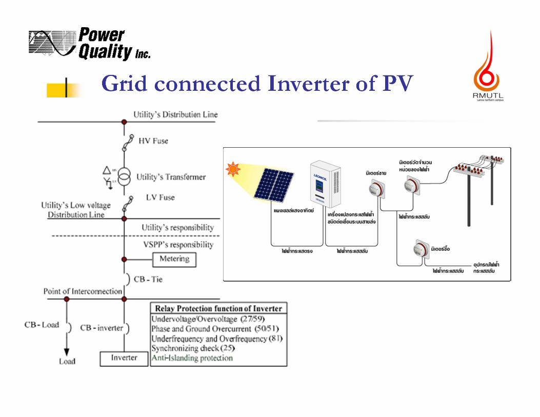
Grid connected Inverter of PV
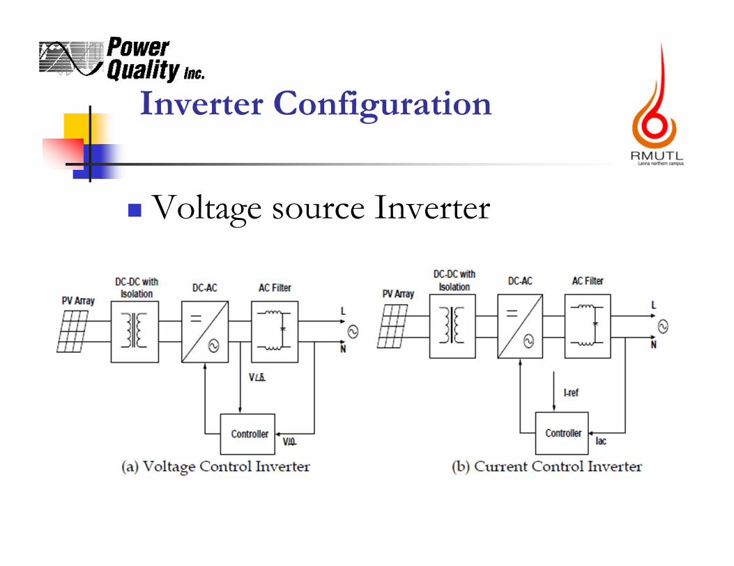
Inverter Configuration
Voltage source Inverter
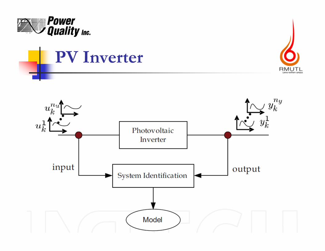
PV Inverter
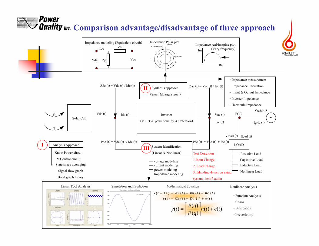
Comparison advantage/disadvantage of three approach
Synthesis approach
(Small&Large signal)
Inverter
(MPPT & power quality &protection)
Vdc (t) Idc (t) Vac (t)
Iac (t)
Pdc (t) = Vdc (t) x Idc (t) Pac (t) = Vac (t) x Iac (t)
Zdc (t) = Vdc (t) / Idc (t) Zac (t) = Vac (t) / Iac (t)
System Identification
(Linear & Nonlinear)
Solar CellG
T
~
LOAD
Vgrid (t)
Igrid (t)
Vload (t) Iload (t)
PCC
voltage modelingcurrent modelingpower modelingImpedance modeling
Resistive Load
Capasitive LoadInductive Load
Nonlinear Load
III
II
- Impedance measurement
- Impedance Caculation
- Input & Output Impedance
- Inverter Impedance
- Harmonic Impedance
Re
ImImpedance real-imagine plot
Impedance Polar plotImpedance modeling (Equivalent circuit)
I Analysis Approach
Know Power circuit
& Control circuitState space averaging
Signal flow graph
Bond graph theory
(Vary frequency)
0.025 0.03 0.035 0.04 0.045 0.05-400
-300
-200
-100
0
100
200
300
400
Time
Measured and simulated model output
Best fits 98.05%
)()()()()()()()(
tetDutCxtytKetButAxTstx
)()()()()( tetu
qFqBty
Linear Tool Analysis Simulation and Prediction Mathematical Equation
- Function Analysis
- Chaos
- Bifurcation
- Irreveribility
Nonlinear Analysis
Zp
ZsIdc
Vdc Vac
phase
magnitude
Z (Impedance)
Test Condition
1.Input Change
2. Load Change
3. Islanding detection using
system identification
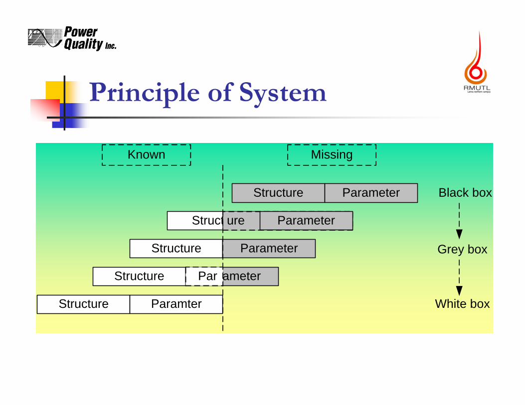
Principle of System
Structureure
Structure Parameter
Parameter
Structure Parameter
Structure Parameter
Structure Paramter
Par
Known Missing
Black box
Grey box
White box
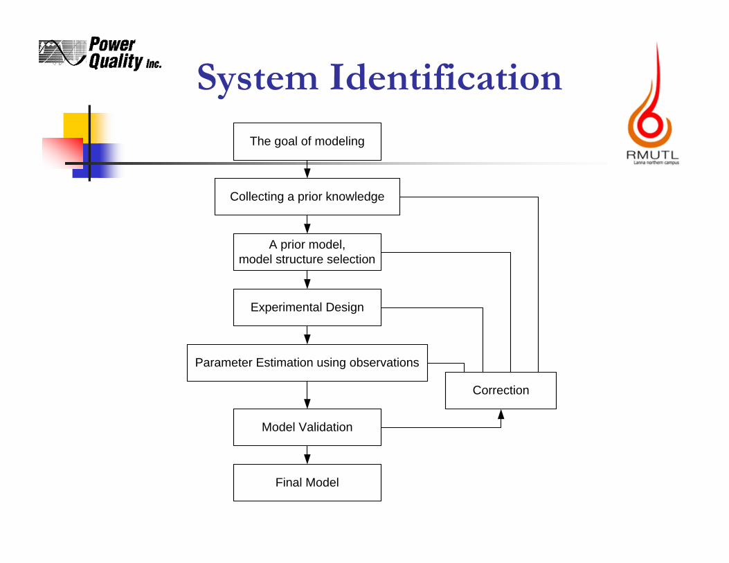
System Identification
The goal of modeling
Model Validation
Parameter Estimation using observations
Experimental Design
A prior model, model structure selection
Collecting a prior knowledge
Final Model
Correction

Type of System Identification
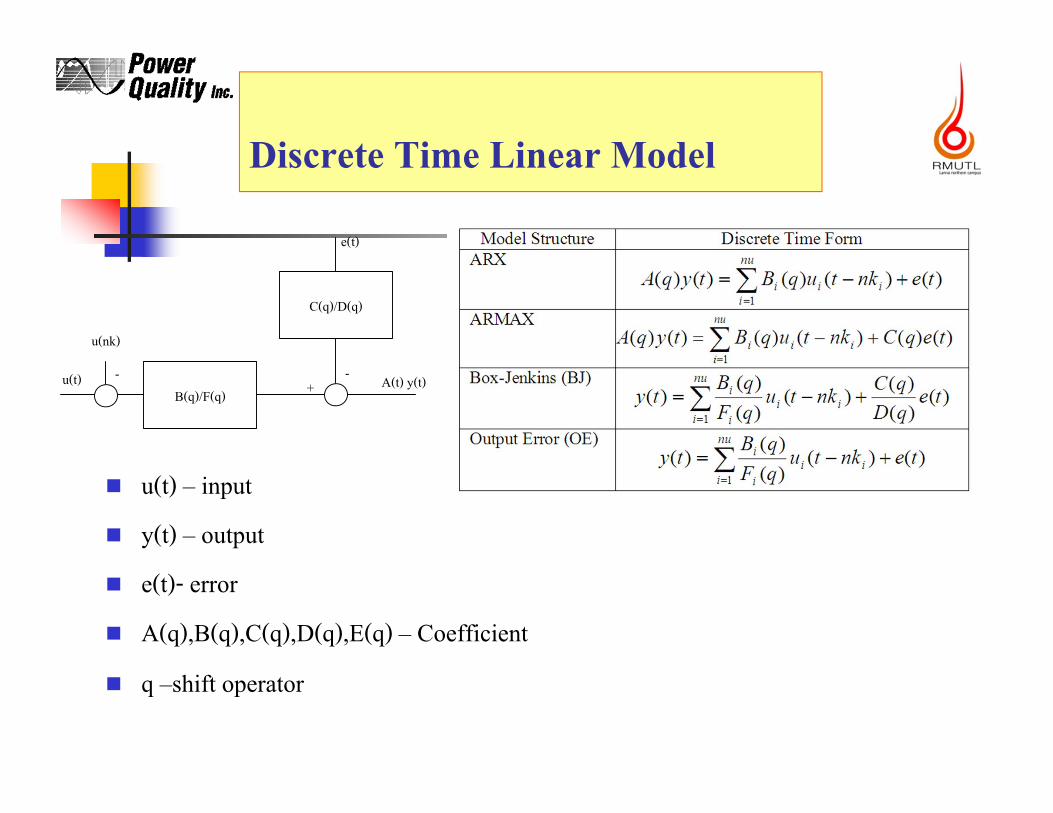
Discrete Time Linear Model
u(t) – input
y(t) – output
e(t)- error
A(q),B(q),C(q),D(q),E(q) – Coefficient
q –shift operator
B(q)/F(q)
C(q)/D(q)
A(t) y(t)u(t)
e(t)
-+
u(nk)
-
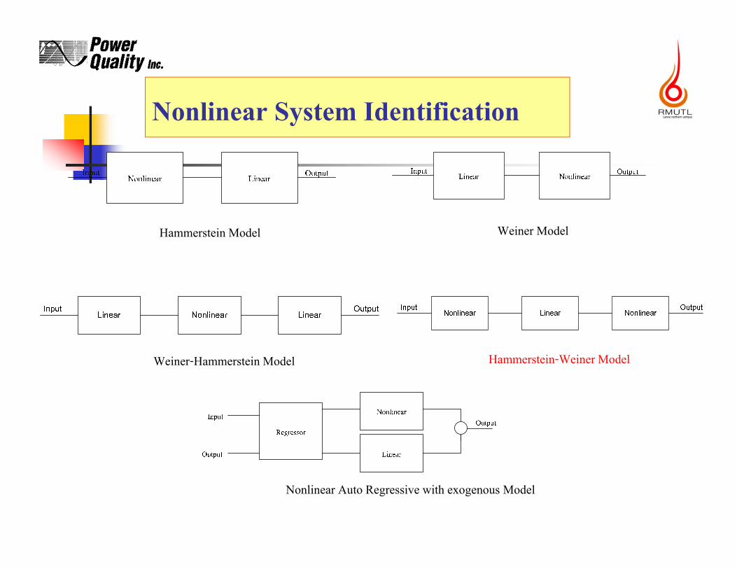
Nonlinear System Identification
Hammerstein Model Weiner Model
Hammerstein-Weiner ModelWeiner-Hammerstein Model
Nonlinear Auto Regressive with exogenous Model
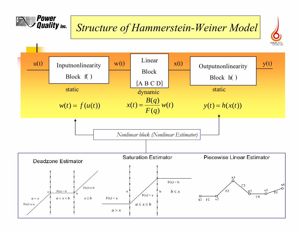
Structure of Hammerstein-Weiner Model
Inputnonlinearity
Block f( )
Linear
Block
[A B C D]
Outputnonlinearity
Block h( )
u(t) y(t)w(t) x(t)
static staticdynamic
))(()( tuftw )()()()( tw
qFqBtx ))(()( txhty
a bF(x) = 0
F(x)=x-b
F(x)=x-a
bxa xa bx
a bF(x) = x
F(x) = b
F(x) = a
xa
xb
bxa
Nonlinear block (Nonlinear Estimator)
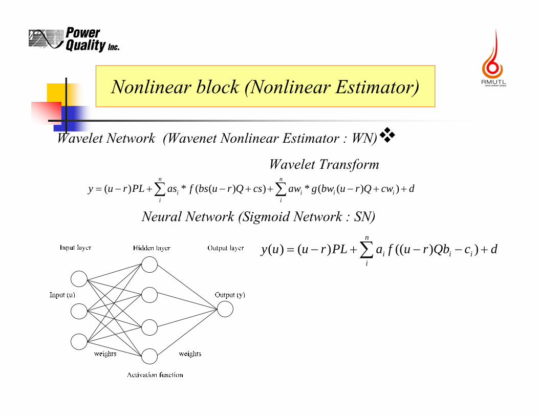
Nonlinear block (Nonlinear Estimator)
Wavelet Network (Wavenet Nonlinear Estimator : WN)
Wavelet Transform
Neural Network (Sigmoid Network : SN)
dcQbrufaPLruuyn
iiii ))(()()(
dcwQrubwgawcsQrubsfasPLruyn
iiii
n
ii ))((*))((*)(
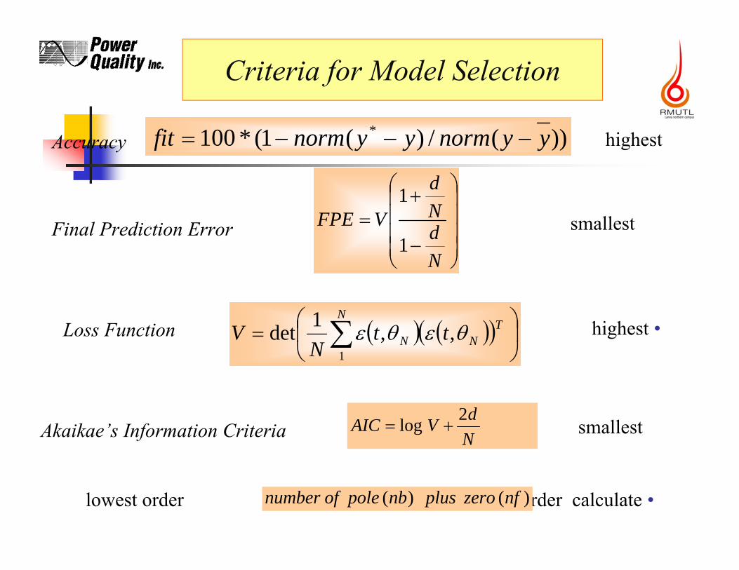
Criteria for Model Selection
))(/)(1(*100 * yynormyynormfit
NdNd
VFPE1
1
NT
NN ttN
V1
,,1det
Final Prediction Error
Loss Function
Accuracy
NdVAIC 2log Akaikae’s Information Criteria
•highest
highest
smallest
smallest
•Model order calculate lowest order )()( nfzeroplusnbpoleofnumber

Research Methodology

Testing inverter
Frobius IG 1500 WLeonics Apollo G300 5000 W
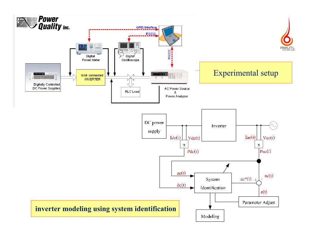
Experimental setup
inverter modeling using system identification
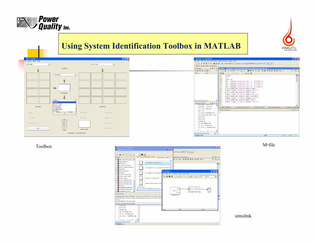
Using System Identification Toolbox in MATLAB
M-file
simulink
Toolbox
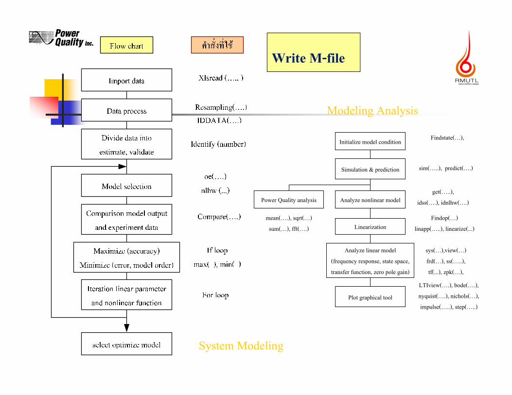
Analyze nonlinear modelget(…..),
idss(….), idnlhw(….)
Simulation & prediction
Findstate(…),
LinearizationFindop(…)
linapp(…..), linearize(...)
Analyze linear model
(frequency response, state space,
transfer function, zero pole gain)
Initialize model condition
sim(…..), predict(….)
sys(…),view(…)
frd(…), ss(…..),
tf(...), zpk(…),
Plot graphical tool
LTIview(….), bode(….),
nyquist(….), nichols(…),
impulse(…..), step(…..)
Power Quality analysis
mean(….), sqrt(…)
sum(…), fft(….)
System Modeling
Modeling Analysis
Write M-file
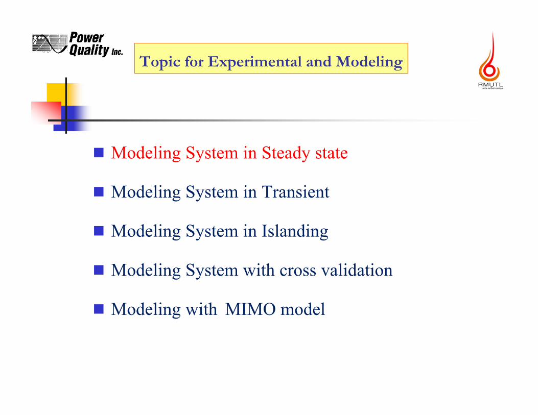
Topic for Experimental and Modeling
Modeling System in Steady state
Modeling System in Transient
Modeling System in Islanding
Modeling System with cross validation
Modeling with MIMO model
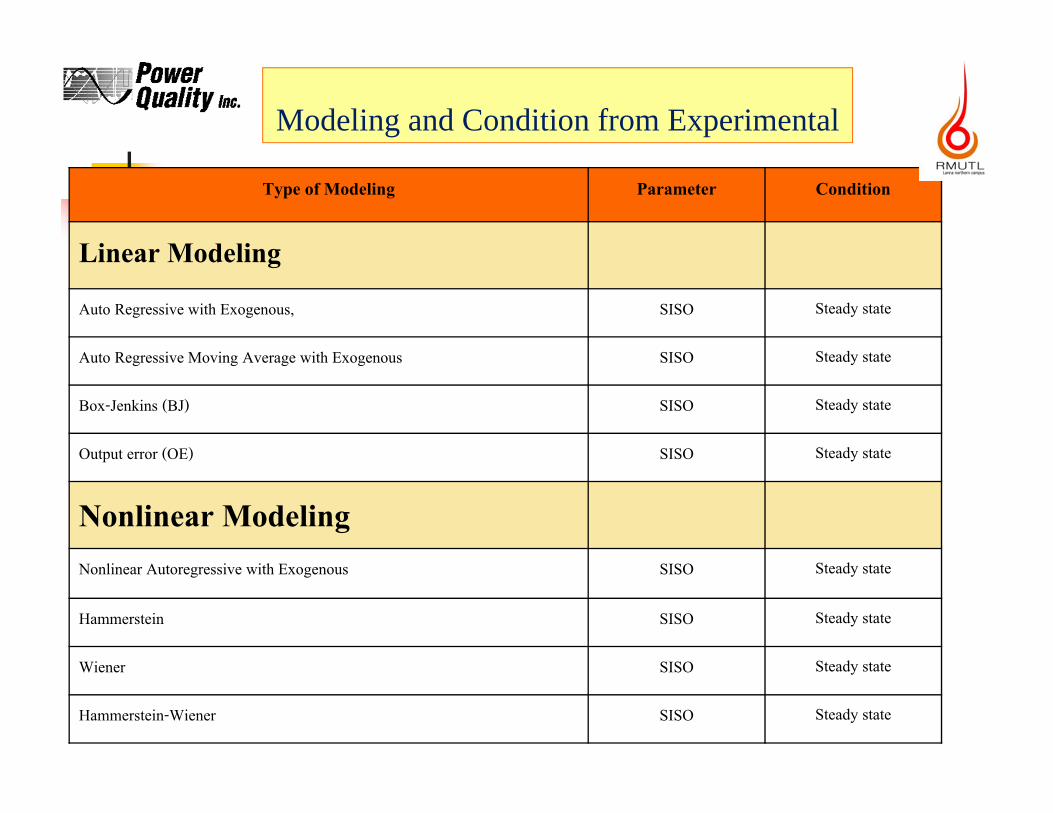
Type of Modeling Parameter Condition
Linear Modeling
Auto Regressive with Exogenous, SISO Steady state
Auto Regressive Moving Average with Exogenous SISO Steady state
Box-Jenkins (BJ) SISO Steady state
Output error (OE) SISO Steady state
Nonlinear ModelingNonlinear Autoregressive with Exogenous SISO Steady state
Hammerstein SISO Steady state
Wiener SISO Steady state
Hammerstein-Wiener SISO Steady state
Modeling and Condition from Experimental
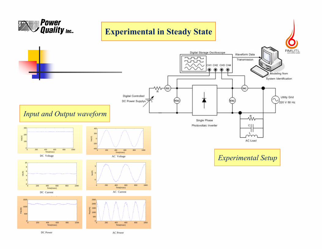
Experimental in Steady State
0 200 400 600 800 10000
100
200
300
Vdc
(V)
Time(msec)
0 200 400 600 800 10000
2
4
6
8
10
Idc(
A)
Time(msec)
0 200 400 600 800 1000-400
-200
0
200
400
Vac
(V)
Time(msec)
0 200 400 600 800 1000
-5
0
5
Iac(
A)
Time(msec)
( )
0 200 400 600 800 10000
500
1000
1500
Pdc
(W)
Time(msec)0 200 400 600 800 1000
0
500
1000
1500
2000
2500
Pac
(VA
)
Time(msec)
DC Voltage AC Voltage
DC Current AC Current
DC Power AC Power
Input and Output waveform
Experimental Setup
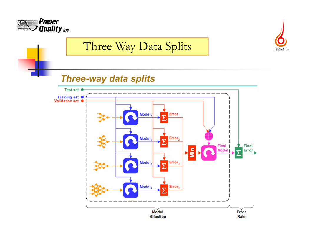
Three Way Data Splits
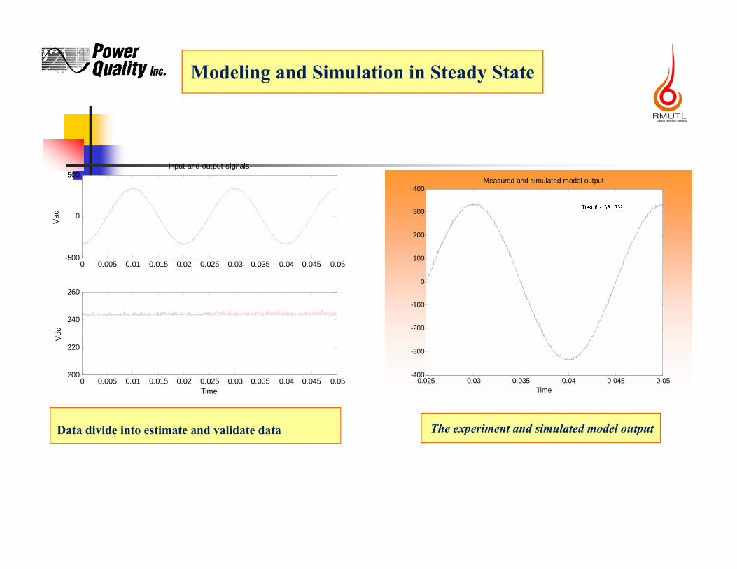
Data divide into estimate and validate data
0 0.005 0.01 0.015 0.02 0.025 0.03 0.035 0.04 0.045 0.05-500
0
500
Vac
Input and output signals
0 0.005 0.01 0.015 0.02 0.025 0.03 0.035 0.04 0.045 0.05200
220
240
260
Time
Vdc
0.025 0.03 0.035 0.04 0.045 0.05-400
-300
-200
-100
0
100
200
300
400
Time
Measured and simulated model output
The experiment and simulated model output
Modeling and Simulation in Steady State
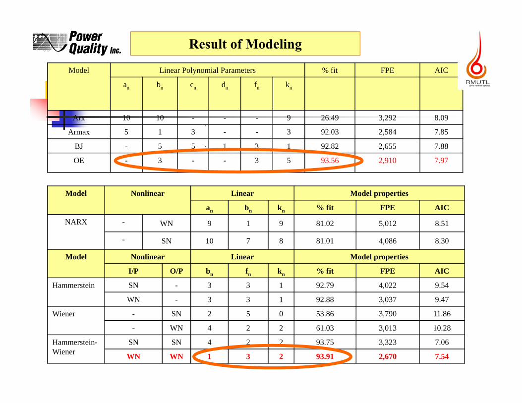
Model Linear Polynomial Parameters % fit FPE AIC
an bn cn dn fn kn
Arx 10 10 - - - 9 26.49 3,292 8.09
Armax 5 1 3 - - 3 92.03 2,584 7.85
BJ - 5 5 1 3 1 92.82 2,655 7.88
OE - 3 - - 3 5 93.56 2,910 7.97
Result of Modeling
Model Nonlinear Linear Model properties
an bn kn % fit FPE AIC
NARX - WN 9 1 9 81.02 5,012 8.51
- SN 10 7 8 81.01 4,086 8.30
Model Nonlinear Linear Model properties
I/P O/P bn fn kn % fit FPE AIC
Hammerstein SN - 3 3 1 92.79 4,022 9.54
WN - 3 3 1 92.88 3,037 9.47
Wiener - SN 2 5 0 53.86 3,790 11.86
- WN 4 2 2 61.03 3,013 10.28
Hammerstein-Wiener
SN SN 4 2 2 93.75 3,323 7.06
WN WN 1 3 2 93.91 2,670 7.54
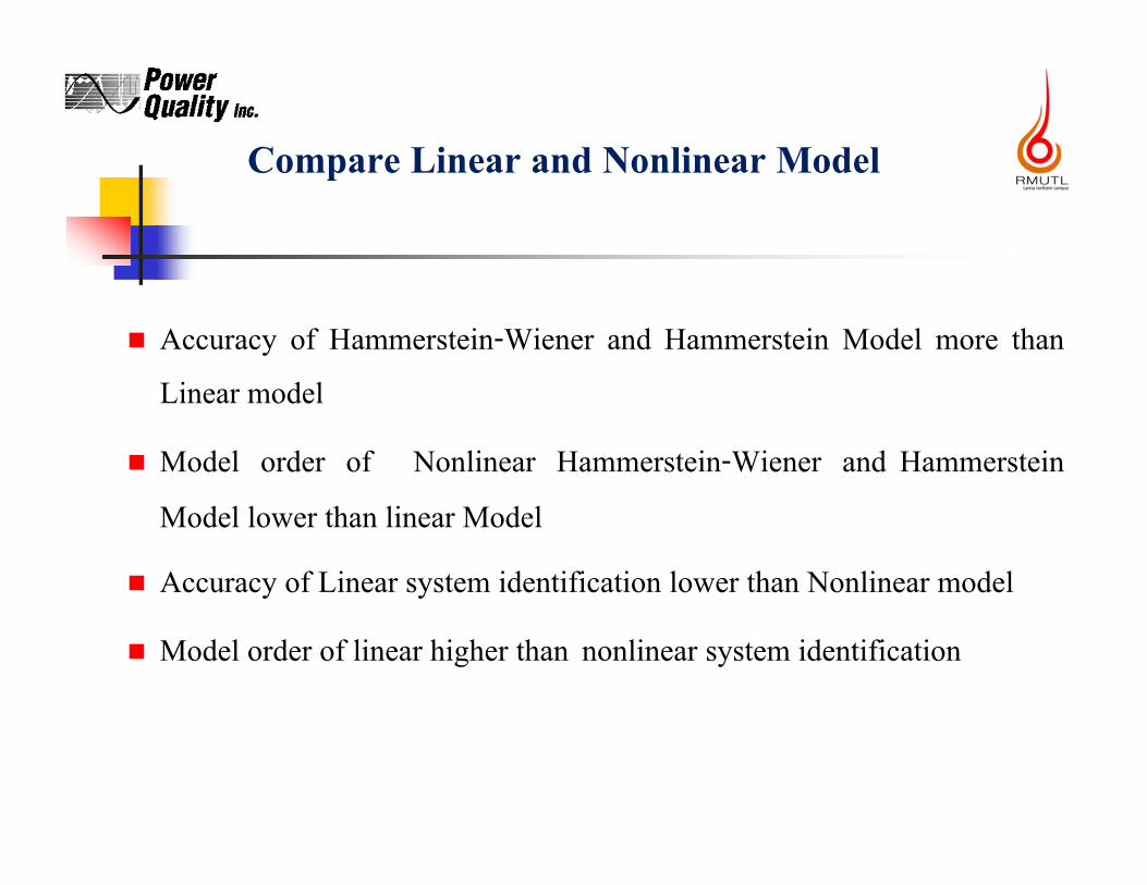
Compare Linear and Nonlinear Model
Accuracy of Hammerstein-Wiener and Hammerstein Model more than
Linear model
Model order of Nonlinear Hammerstein-Wiener and Hammerstein
Model lower than linear Model
Accuracy of Linear system identification lower than Nonlinear model
Model order of linear higher than nonlinear system identification
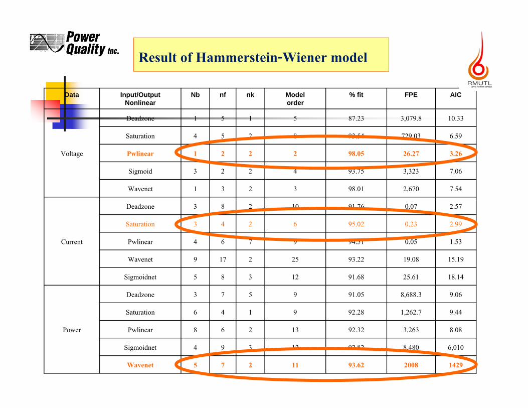
Result of Hammerstein-Wiener model
Data Input/Output Nonlinear
Nb nf nk Modelorder
% fit FPE AIC
Voltage
Deadzone 1 5 1 5 87.23 3,079.8 10.33
Saturation 4 5 2 8 93.54 729.03 6.59
Pwlinear 1 2 2 2 98.05 26.27 3.26
Sigmoid 3 2 2 4 93.75 3,323 7.06
Wavenet 1 3 2 3 98.01 2,670 7.54
Current
Deadzone 3 8 2 10 91.76 0.07 2.57
Saturation 3 4 2 6 95.02 0.23 2.99
Pwlinear 4 6 7 9 94.51 0.05 1.53
Wavenet 9 17 2 25 93.22 19.08 15.19
Sigmoidnet 5 8 3 12 91.68 25.61 18.14
Power
Deadzone 3 7 5 9 91.05 8,688.3 9.06
Saturation 6 4 1 9 92.28 1,262.7 9.44
Pwlinear 8 6 2 13 92.32 3,263 8.08
Sigmoidnet 4 9 3 12 92.82 8,480 6,010
Wavenet 5 7 2 11 93.62 2008 1429
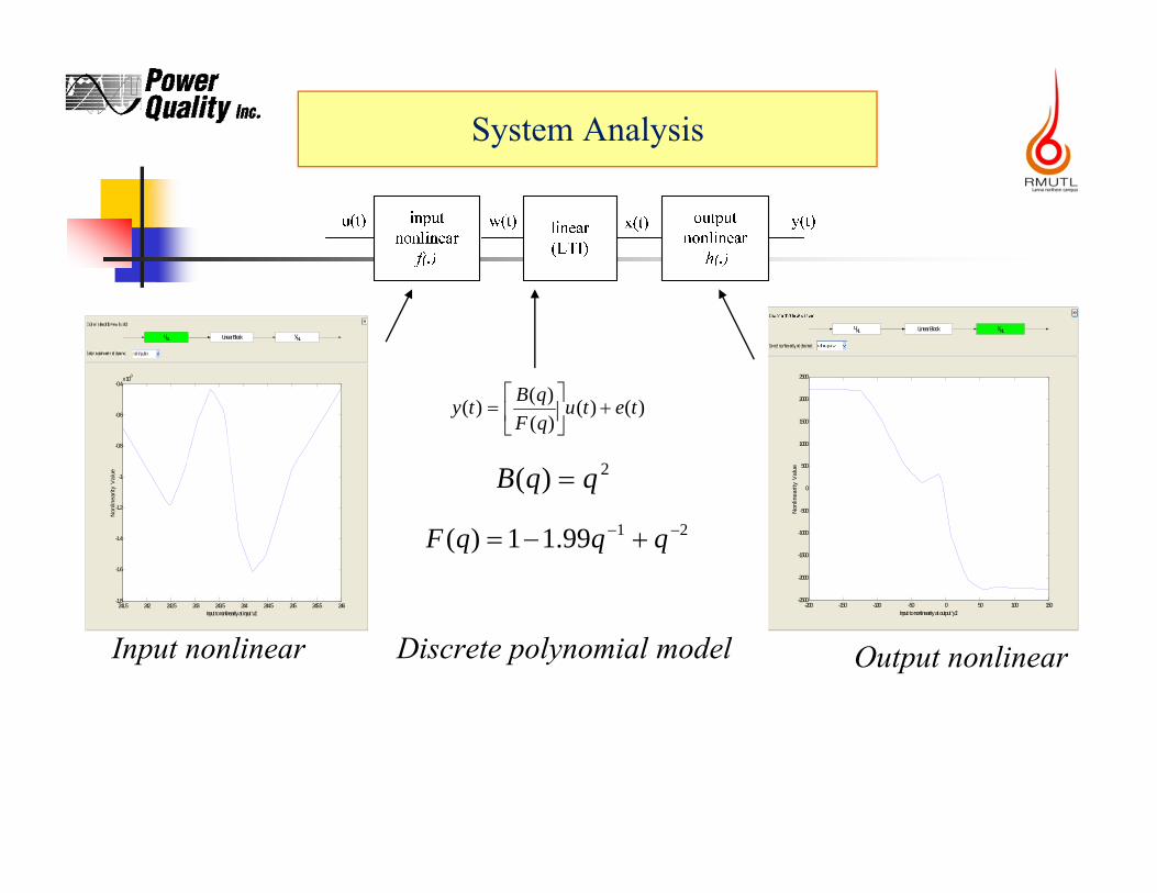
System Analysis
)()()()()( tetu
qFqBty
2)( qqB
2199.11)( qqqF
Discrete polynomial modelInput nonlinear Output nonlinear
uNL Linear Block yNL
241.5 242 242.5 243 243.5 244 244.5 245 245.5 246-1.8
-1.6
-1.4
-1.2
-1
-0.8
-0.6
-0.4x 10⁻³
Input to nonlinearity at input 'u1'
Non
linea
rity
Val
ue
uNL Linear Block yNL
-200 -150 -100 -50 0 50 100 150-2500
-2000
-1500
-1000
-500
0
500
1000
1500
2000
2500
Input to nonlinearity at output 'y1'
Non
linea
rity
Val
ue
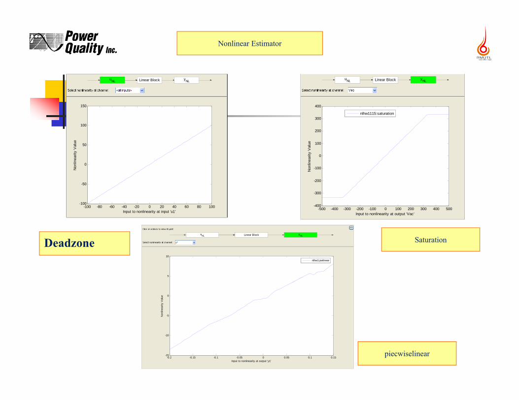
Deadzone
uNL Linear Block yNL
-100 -80 -60 -40 -20 0 20 40 60 80 100-100
-50
0
50
100
150
Input to nonlinearity at input 'u1'
Non
linea
rity
Val
ue
uNL Linear Block yNL
-500 -400 -300 -200 -100 0 100 200 300 400 500-400
-300
-200
-100
0
100
200
300
400
Input to nonlinearity at output 'Vac'
Non
linea
rity
Val
ue
nlhw1115:saturation
SaturationuNL Linear Block yNL
-0.2 -0.15 -0.1 -0.05 0 0.05 0.1 0.15-15
-10
-5
0
5
10
Input to nonlinearity at output 'y1'
Non
linea
rity
Val
ue
nlhw1:pwlinear
piecwiselinear
Nonlinear Estimator
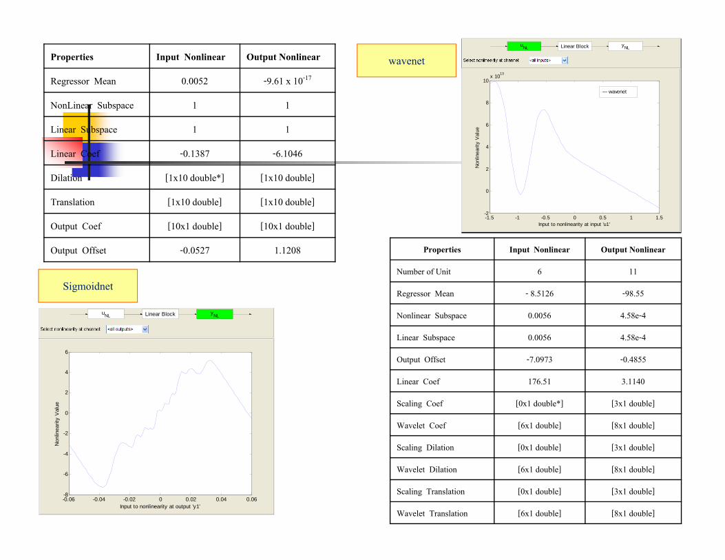
Properties Input Nonlinear Output Nonlinear
Regressor Mean 0.0052 -9.61 x 10⁻¹⁷
NonLinear Subspace 1 1
Linear Subspace 1 1
Linear Coef -0.1387 -6.1046
Dilation [1x10 double*] [1x10 double]
Translation [1x10 double] [1x10 double]
Output Coef [10x1 double] [10x1 double]
Output Offset -0.0527 1.1208
uNL Linear Block yNL
-0.06 -0.04 -0.02 0 0.02 0.04 0.06-8
-6
-4
-2
0
2
4
6
Input to nonlinearity at output 'y1'
Non
linea
rity
Val
ue
Properties Input Nonlinear Output Nonlinear
Number of Unit 6 11
Regressor Mean - 8.5126 -98.55
Nonlinear Subspace 0.0056 4.58e-4
Linear Subspace 0.0056 4.58e-4
Output Offset -7.0973 -0.4855
Linear Coef 176.51 3.1140
Scaling Coef [0x1 double*] [3x1 double]
Wavelet Coef [6x1 double] [8x1 double]
Scaling Dilation [0x1 double] [3x1 double]
Wavelet Dilation [6x1 double] [8x1 double]
Scaling Translation [0x1 double] [3x1 double]
Wavelet Translation [6x1 double] [8x1 double]
uNL Linear Block yNL
-1.5 -1 -0.5 0 0.5 1 1.5-2
0
2
4
6
8
10x 10
13
Input to nonlinearity at input 'u1'
Non
linea
rity
Val
ue
--- wavenet
wavenet
Sigmoidnet
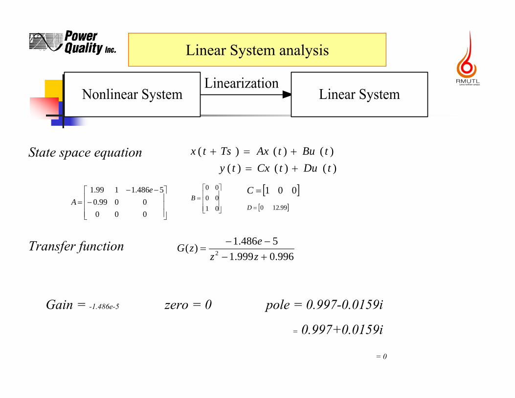
)()()()()()(tDutCxtytButAxTstx
State space equation
0000099.0
5486.1199.1 eA
001C
Transfer function
Gain = -1.486e-5 pole = 0.997-0.0159i
= 0.997+0.0159i
= 0
zero = 0
996.0999.15486.1)( 2
zzezG
010000
B 99.120D
Linear System analysis
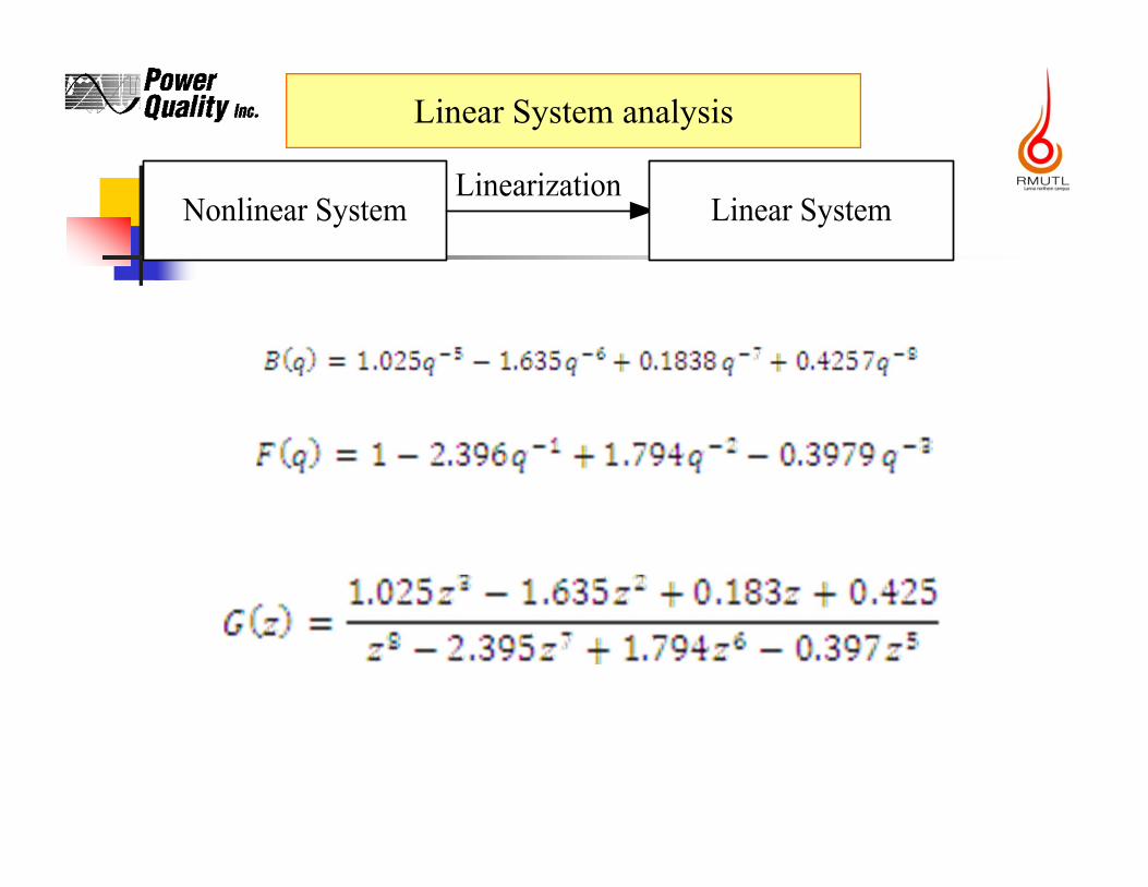
Linear System analysis
Pole-Zero Map
Real Axis
Imag
inar
y Ax
is
Nichols Chart
Open-Loop Phase (deg)
Ope
n-Lo
op G
ain
(dB)
Nyquist Diagram
Real Axis
Imag
inar
y Ax
is
Time (sec)
Ampl
itude
Time (sec)
Ampl
itude
Frequency (rad/sec)
-1 -0.5 0 0.5 1-1
-0.8
-0.6
-0.4
-0.2
0
0.2
0.4
0.6
0.8
1
/T
0.1/T
0.2/T
0.3/T0.4/T0.5/T0.6/T
0.7/T
0.8/T
0.9/T
/T
0.10.20.30.40.50.60.70.80.9
From: u1 To: y1
0.1/T
0.2/T
0.3/T0.4/T0.5/T0.6/T
0.7/T
0.8/T
0.9/T
-180 -90 0 90 180-120
-100
-80
-60
-40
-20
0
20
40From: u1 To: y1
6 dB 3 dB 1 dB 0.5 dB
0.25 dB 0 dB
-1 dB -3 dB -6 dB -12 dB -20 dB
-40 dB
-60 dB
-80 dB
-100 dB
-120 dB-1.5 -1 -0.5 0 0.5 1 1.5
-2.5
-2
-1.5
-1
-0.5
0
0.5
1
1.5
2
2.5From: u1 To: y1
0 dB
-20 dB-10 dB
-6 dB
-4 dB
-2 dB
20 dB10 dB
6 dB
4 dB
2 dB
0 200 400 600 800 1000 1200 1400-1
-0.8
-0.6
-0.4
-0.2
0
0.2
0.4
0.6
0.8
1x 10
-3 From: u1 To: y1
0 200 400 600 800 1000 1200-0.12
-0.1
-0.08
-0.06
-0.04
-0.02
0From: u1 To: y1
10-2
10-1
100
101
102
-180
-90
0
90
180
Phas
e (d
eg)
-150
-100
-50
0
50From: u1 To: y1
Mag
nitu
de (d
B)
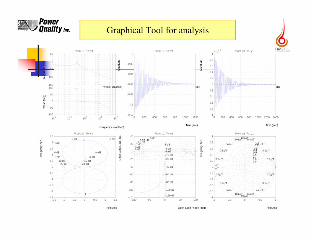
Graphical Tool for analysis
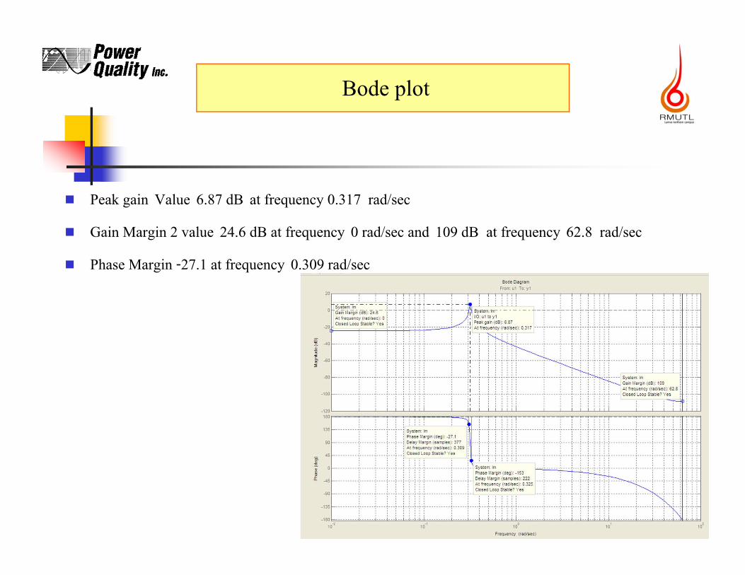
Peak gain Value 6.87 dB at frequency 0.317 rad/sec
Gain Margin 2 value 24.6 dB at frequency 0 rad/sec and 109 dB at frequency 62.8 rad/sec
Phase Margin -27.1 at frequency 0.309 rad/sec
Bode plot
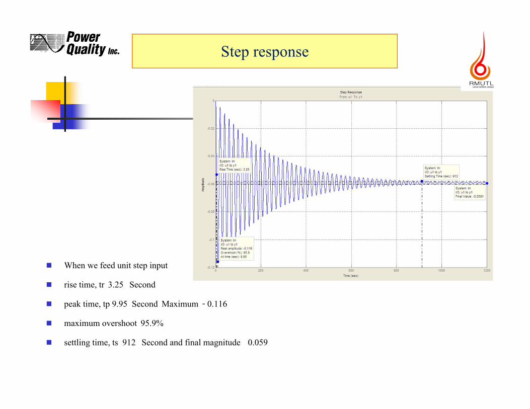
When we feed unit step input
rise time, tr 3.25 Second
peak time, tp 9.95 Second Maximum - 0.116
maximum overshoot 95.9% settling time, ts 912 Second and final magnitude 0.059
Step response

Amplitude -0.000915 at time 4.95 and steady state time 917 second
Impulse response

Peak gain = 6.87 dB at frequency 0.317 rad/s
Gain margin 2 values are 24.6 dB at frequency 0 rad/sec and 109 dB at frequency 62.8 rad/sec
Phase margin 2 values are -27.1 degree at frequency 0.309 rad/sec and -153 degree at frequency 0.325 rad/sec
Nyquist Analysis
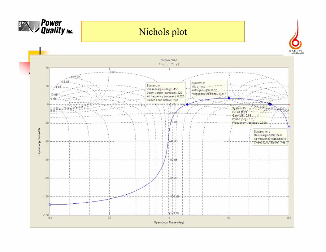
Nichols plot
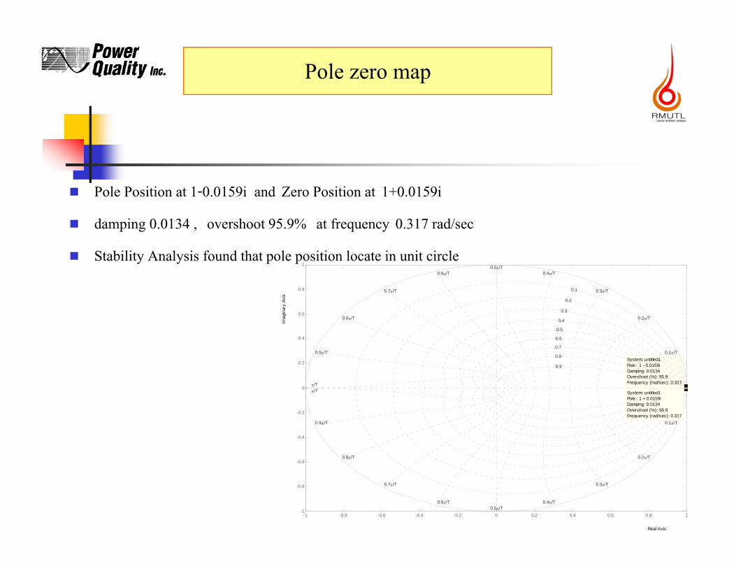
Pole Position at 1-0.0159i and Zero Position at 1+0.0159i
damping 0.0134 , overshoot 95.9% at frequency 0.317 rad/sec
Stability Analysis found that pole position locate in unit circle
Real Axis
Imag
inar
y Ax
is
-1 -0.8 -0.6 -0.4 -0.2 0 0.2 0.4 0.6 0.8 1-1
-0.8
-0.6
-0.4
-0.2
0
0.2
0.4
0.6
0.8
1
System: untitled1Pole : 1 - 0.0159iDamping: 0.0134Overshoot (%): 95.9Frequency (rad/sec): 0.317
0.1/T
0.2/T
0.3/T
0.4/T0.5/T
0.6/T
0.7/T
0.8/T
0.9/T
/T
0.1/T
0.2/T
0.3/T
0.4/T0.5/T
0.6/T
0.7/T
0.8/T
0.9/T
/T
0.1
0.2
0.3
0.4
0.5
0.6
0.7
0.8
0.9
System: untitled1Pole : 1 + 0.0159iDamping: 0.0134Overshoot (%): 95.9Frequency (rad/sec): 0.317
Pole zero map
Linear system Stability analysis
Nonlinear Linear Linearization around operating point Steady State condition Stability analysis
Linear system Stability analysis
Right hand plane (RHP) Root locus, Routh – Hurwitz criterion Z plane and Unit circle Eigenvalue of Jacobian matrix Lyapunov Bode-Nyquist stability criterion
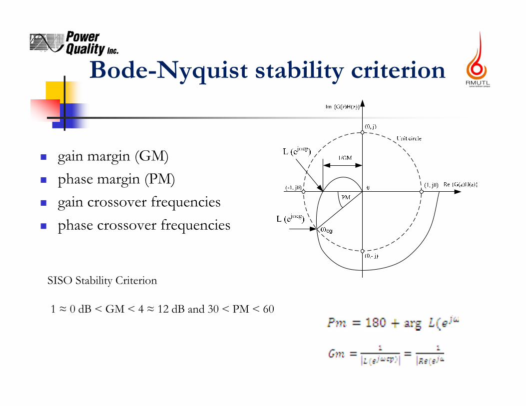
Bode-Nyquist stability criterion
gain margin (GM) phase margin (PM) gain crossover frequencies phase crossover frequencies
SISO Stability Criterion
1 ≈ 0 dB < GM < 4 ≈ 12 dB and 30 < PM < 60
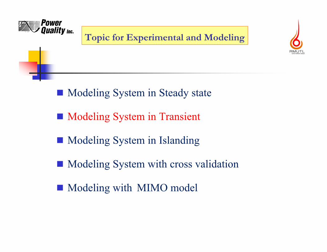
Topic for Experimental and Modeling
Modeling System in Steady state
Modeling System in Transient
Modeling System in Islanding
Modeling System with cross validation
Modeling with MIMO model
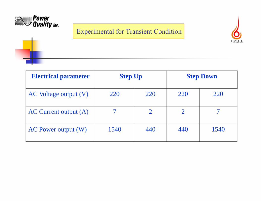
Electrical parameter Step Up Step Down
AC Voltage output (V) 220 220 220 220
AC Current output (A) 7 2 2 7
AC Power output (W) 1540 440 440 1540
Experimental for Transient Condition

Power dc inputPower ac output
0 1000 2000 3000 4000 5000 6000 7000 8000 9000 10000-500
0
500
1000
1500
2000
2500
3000
3500
Pac
up(V
A)
Time(msec)
0 1000 2000 3000 4000 5000 6000 7000 8000 9000 10000200
400
600
800
1000
1200
1400
1600
1800
2000
Pdc
up(W
)
Time(msec)
0 1000 2000 3000 4000 5000 6000 7000 8000 9000 10000-500
0
500
1000
1500
2000
2500
3000
3500
Pac
dow
n(W
)
Time(msec)
0 1000 2000 3000 4000 5000 6000 7000 8000 9000 10000400
600
800
1000
1200
1400
1600
1800
2000
Pdc
dow
n(W
)
Time(msec)
Power dc input Power ac output
Step down condition
Step up condition
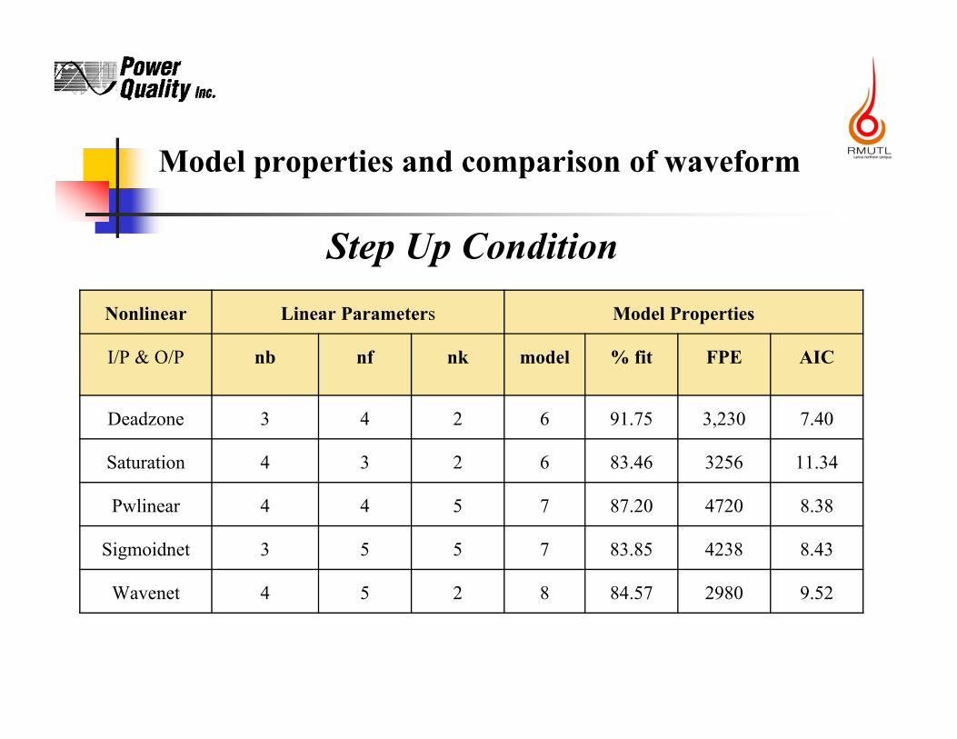
Model properties and comparison of waveform
Step Up ConditionNonlinear Linear Parameters Model Properties
I/P & O/P nb nf nk model % fit FPE AIC
Deadzone 3 4 2 6 91.75 3,230 7.40
Saturation 4 3 2 6 83.46 3256 11.34
Pwlinear 4 4 5 7 87.20 4720 8.38
Sigmoidnet 3 5 5 7 83.85 4238 8.43
Wavenet 4 5 2 8 84.57 2980 9.52
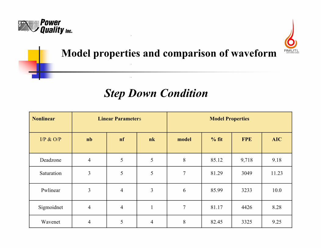
Model properties and comparison of waveform
Step Down Condition
Nonlinear Linear Parameters Model Properties
I/P & O/P nb nf nk model % fit FPE AIC
Deadzone 4 5 5 8 85.12 9,718 9.18
Saturation 3 5 5 7 81.29 3049 11.23
Pwlinear 3 4 3 6 85.99 3233 10.0
Sigmoidnet 4 4 1 7 81.17 4426 8.28
Wavenet 4 5 4 8 82.45 3325 9.25
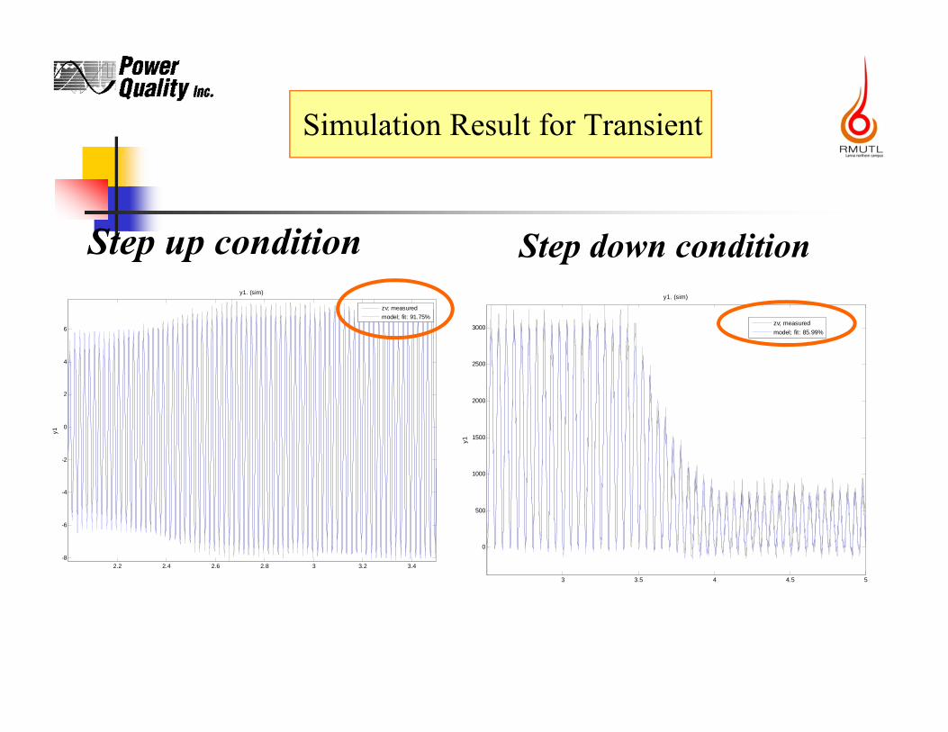
Simulation Result for Transient
2.2 2.4 2.6 2.8 3 3.2 3.4-8
-6
-4
-2
0
2
4
6
y1. (sim)
y1
zv; measuredmodel; fit: 91.75%
Step up condition
3 3.5 4 4.5 5
0
500
1000
1500
2000
2500
3000
y1. (sim)
y1
zv; measuredmodel; fit: 85.99%
Step down condition

Stability Analysis
Pole 4 position follow as
0.9923 + 0.0575i, 0.9923 - 0.0575i, 0.7060 and -0.1213
Real Axis
Imag
inar
y Ax
is
-1 -0.5 0 0.5 1 1.5-1
-0.8
-0.6
-0.4
-0.2
0
0.2
0.4
0.6
0.8
1
0.4/T0.5/T
0.6/T
0.7/T
0.8/T
0.9/T
/T
0.1/T
0.2/T
0.3/T
0.4/T0.5/T
0.6/T
0.7/T
0.8/T
0.9/T
/T
0.1
0.2
0.3
0.4
0.5
0.6
0.7
0.8
0.9
System: untitled1I/O: u1 to y1Pole : 0Damping: NaNOvershoot (%): NaNFrequency (rad/sec): NaN
System: untitled1I/O: u1 to y1Pole : 0.706Damping: 1Overshoot (%): 0Frequency (rad/sec): 696
System: untitled1I/O: u1 to y1Pole : 0.992 + 0.0575iDamping: 0.104Overshoot (%): 71.9Frequency (rad/sec): 116
0.1/T
0.2/T
0.3/T
From: u1 To: y1
System: untitled1I/O: u1 to y1Pole : 0.992 - 0.0575iDamping: 0.104Overshoot (%): 71.9Frequency (rad/sec): 116
•Magnitude are 0.9940, 0.9940, 0.7060 and 0.1213
•Stability : consider from pole position, magnitude of pole and unit cirle
Magnitude of pole < 1
All Pole locate in unit circle
: System is stable
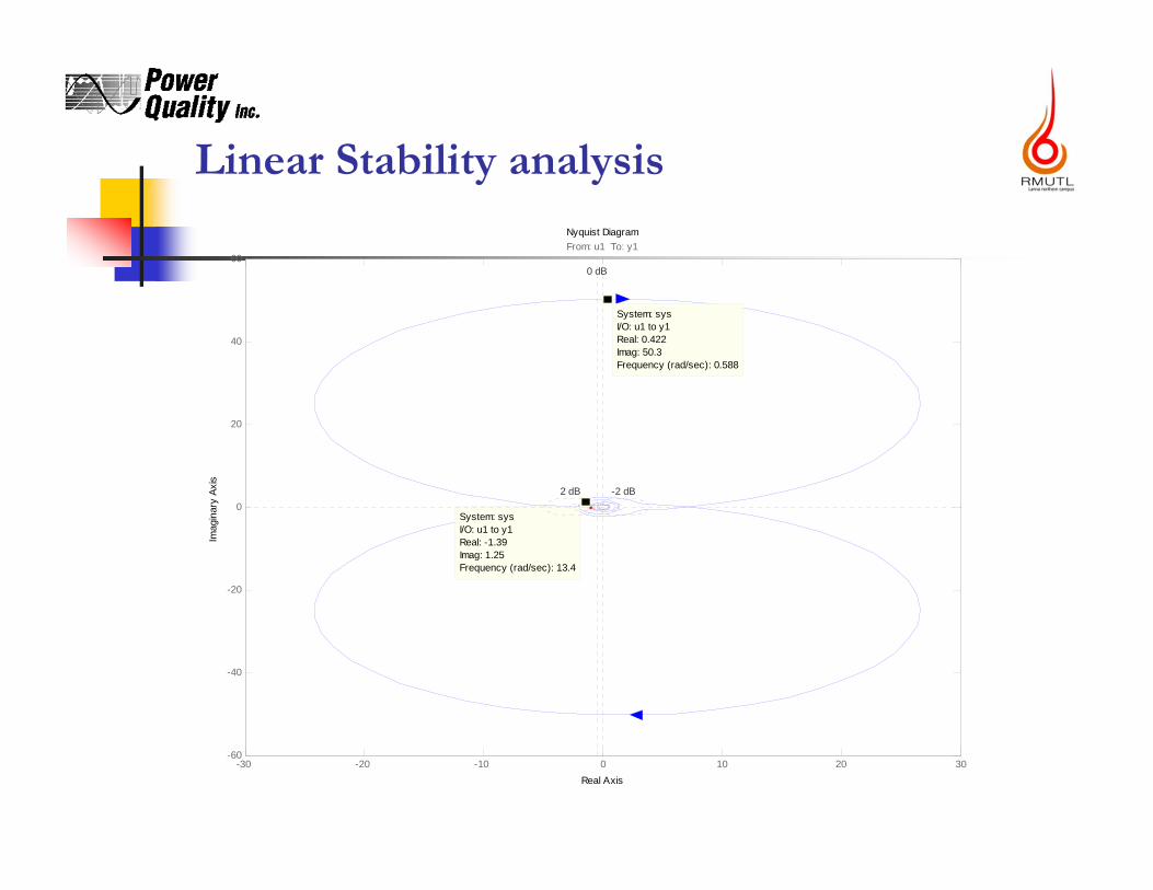
Linear Stability analysisNyquist Diagram
Real Axis
Imag
inar
y Ax
is
-30 -20 -10 0 10 20 30-60
-40
-20
0
20
40
60
System: sysI/O: u1 to y1Real: -1.39Imag: 1.25Frequency (rad/sec): 13.4
System: sysI/O: u1 to y1Real: 0.422Imag: 50.3Frequency (rad/sec): 0.588
0 dB
-2 dB2 dB
From: u1 To: y1
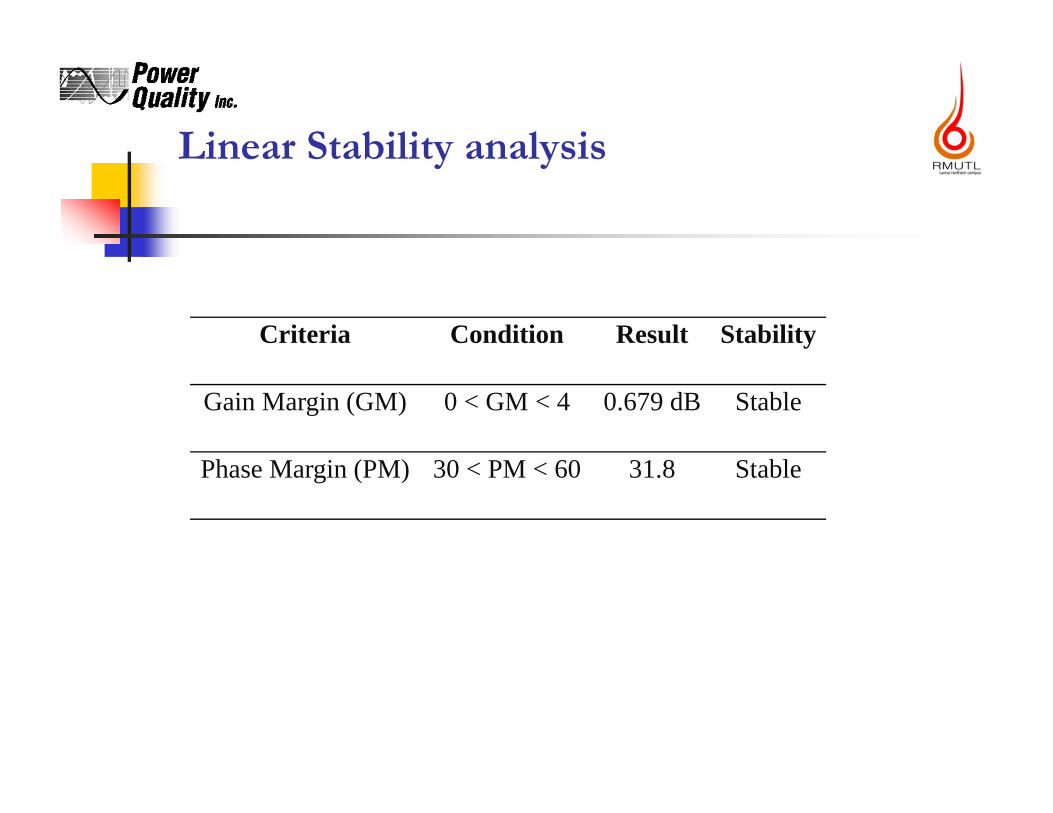
Linear Stability analysis
Criteria Condition Result Stability
Gain Margin (GM) 0 < GM < 4 0.679 dB Stable
Phase Margin (PM) 30 < PM < 60 31.8 Stable
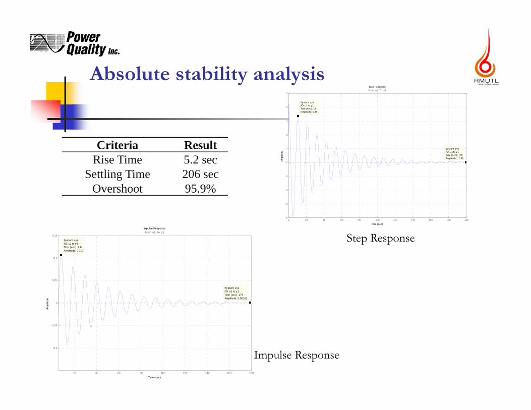
Absolute stability analysis
Criteria ResultRise Time 5.2 sec
Settling Time 206 secOvershoot 95.9%
Step Response
Time (sec)
Ampl
itude
0 20 40 60 80 100 120 140 160 180 200-6
-5
-4
-3
-2
-1
0
1
2
3
System: sysI/O: u1 to y1Time (sec): 199Amplitude: -1.99
System: sysI/O: u1 to y1Time (sec): 11Amplitude: 1.38
From: u1 To: y1
Impulse Response
Time (sec)
Ampl
itude
20 40 60 80 100 120 140 160 180
-0.1
-0.05
0
0.05
0.1
0.15
System: sysI/O: u1 to y1Time (sec): 7.8Amplitude: 0.107
System: sysI/O: u1 to y1Time (sec): 179Amplitude: 0.00101
From: u1 To: y1
Step Response
Impulse Response
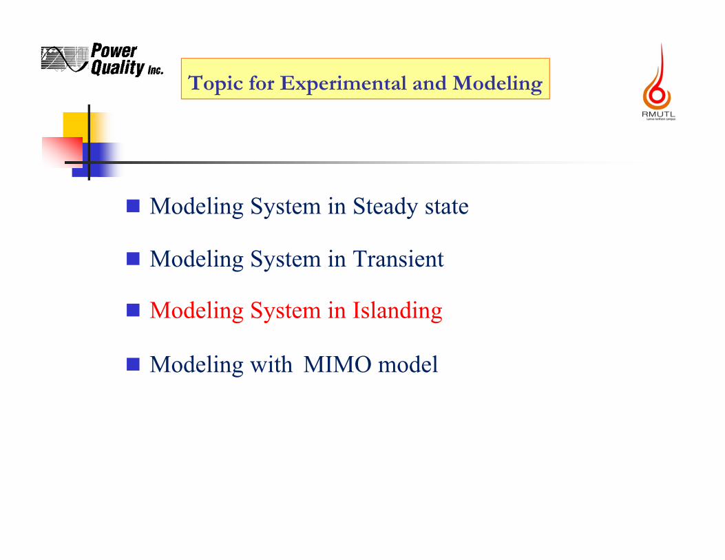
Topic for Experimental and Modeling
Modeling System in Steady state
Modeling System in Transient
Modeling System in Islanding
Modeling with MIMO model
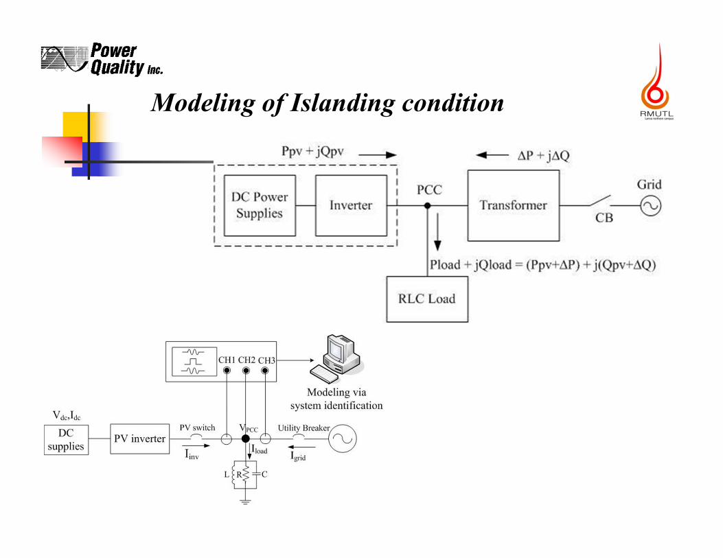
Modeling of Islanding condition
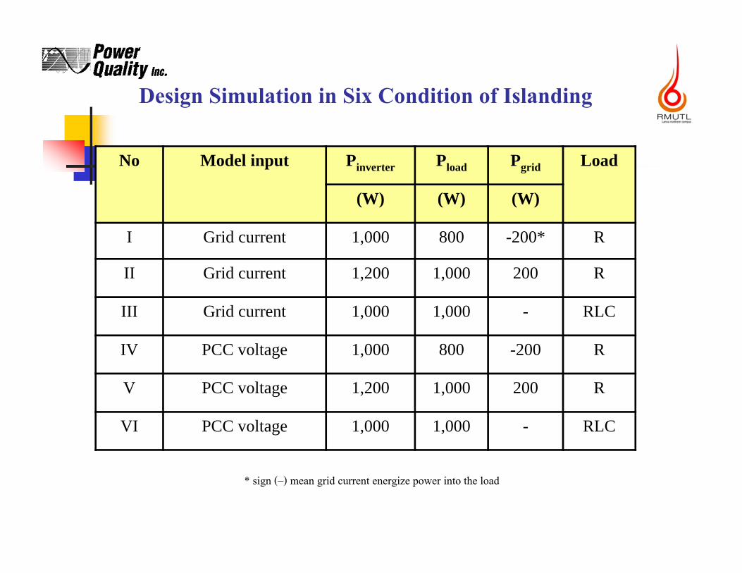
Design Simulation in Six Condition of Islanding
No Model input Pinverter Pload Pgrid Load
(W) (W) (W)
I Grid current 1,000 800 -200* R
II Grid current 1,200 1,000 200 R
III Grid current 1,000 1,000 - RLC
IV PCC voltage 1,000 800 -200 R
V PCC voltage 1,200 1,000 200 R
VI PCC voltage 1,000 1,000 - RLC
* sign (–) mean grid current energize power into the load
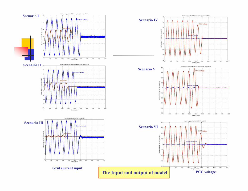
Scenario I
Scenario II
Scenario III
Scenario IV
Scenario V
Scenario VI
The Input and output of modelGrid current input
PCC voltage
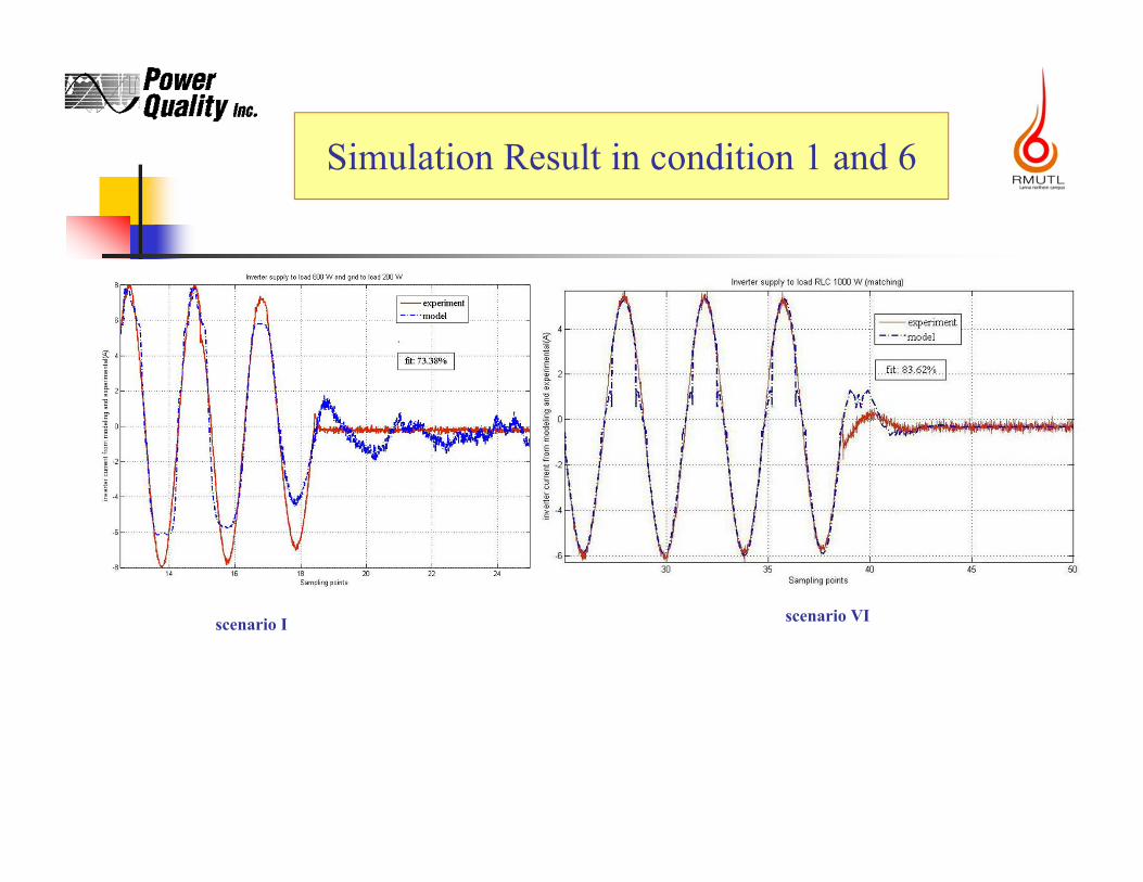
scenario I scenario VI
Simulation Result in condition 1 and 6
Topic for Experimental and Modeling
Modeling System in Steady state
Modeling System in Transient
Modeling System in Islanding
Modeling with MIMO model
)())(()()(
)(
)())(()()()(
)())(()()()(
tetpfqFqB
htp
tetifqFqBhti
tetvfqFqBhtv
dcp
pac
dci
iac
dcv
vac
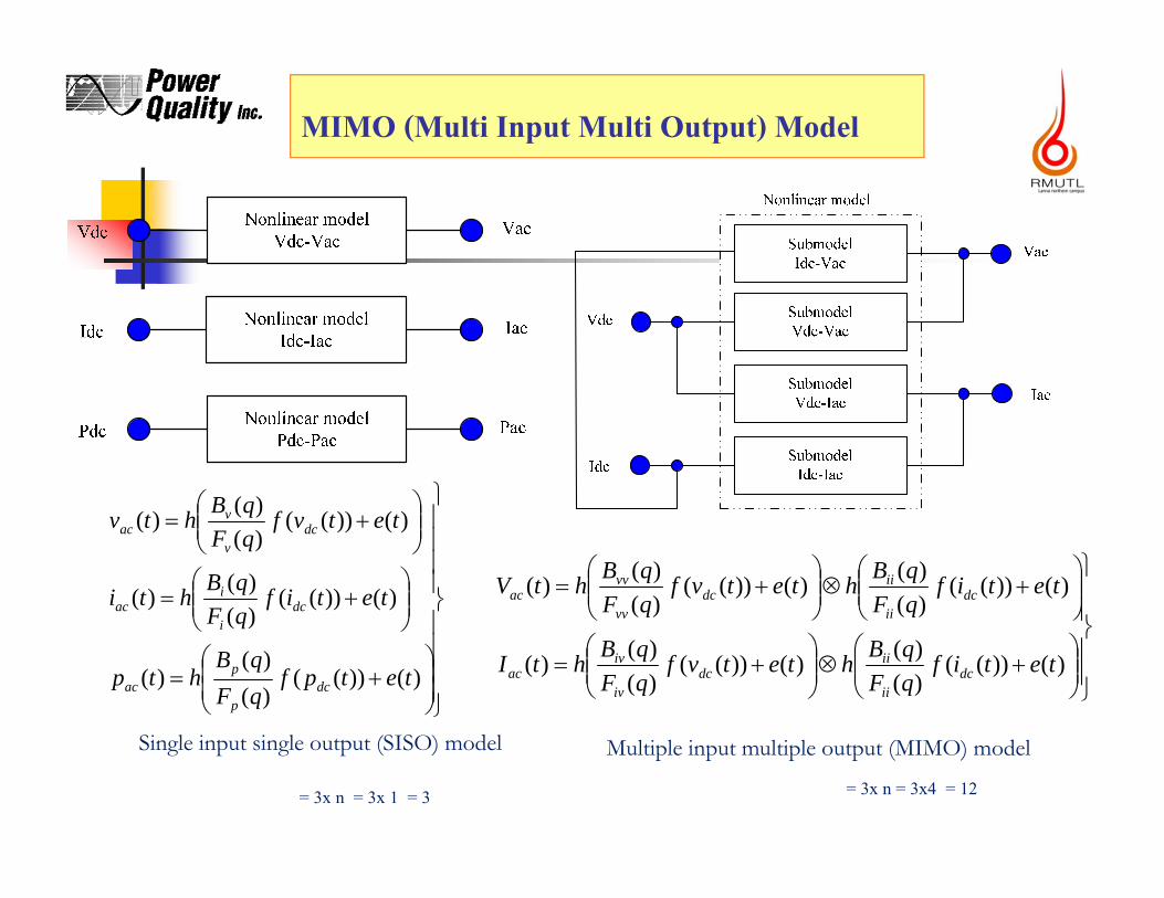
MIMO (Multi Input Multi Output) Model
Single input single output (SISO) model
)())(()()()())((
)()()(
)())(()()()())((
)()()(
tetifqFqBhtetvf
qFqBhtI
tetifqFqBhtetvf
qFqBhtV
dcii
iidc
iv
ivac
dcii
iidc
vv
vvac
Multiple input multiple output (MIMO) model
= 3x n = 3x 1 = 3 = 3x n = 3x4 = 12

SubmodelVdc-Pac
SubmodelIdc-Pac
Idc
Nonlinear model
Pac
Vdc
)())(()()()(
)())(()()()(
tetPfqFqBhtI
tetPfqFqBhtV
dci
iac
dcv
vac
)())((
)()()())((
)()()( tetif
qFqBhtetvf
qFqBhtp dc
i
idc
v
vac
Single input multiple output (SIMO) model Multiple input single output (MISO) model
Number of linear parameter (nb nf nk)
= 3x n ; n = submodel
= 3 x n = 3 x 2 = 6 = 3 x n = 3 x 2 = 6
Structure of Model
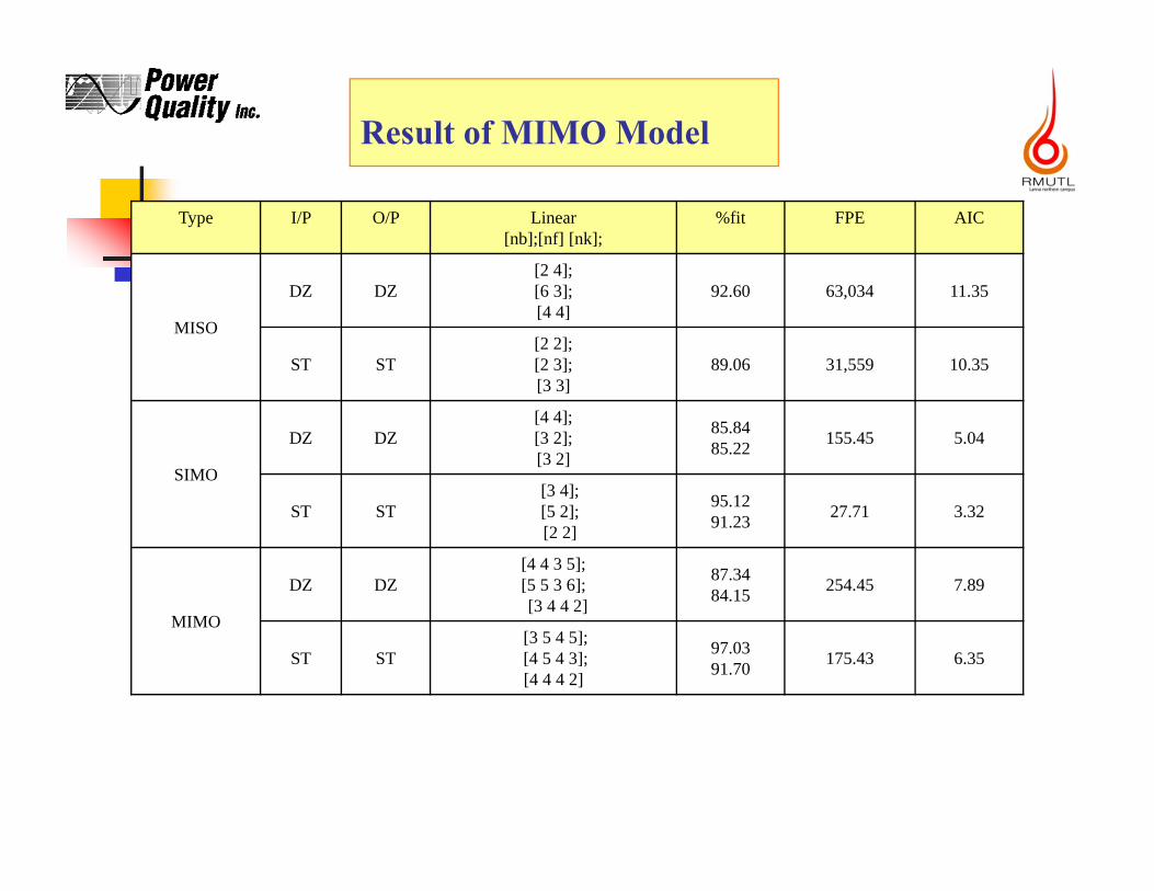
Result of MIMO Model
Type I/P O/P Linear [nb];[nf] [nk];
%fit FPE AIC
MISO
DZ DZ[2 4];[6 3];[4 4]
92.60 63,034 11.35
ST ST[2 2]; [2 3]; [3 3]
89.06 31,559 10.35
SIMO
DZ DZ[4 4]; [3 2]; [3 2]
85.8485.22 155.45 5.04
ST ST[3 4]; [5 2]; [2 2]
95.1291.23 27.71 3.32
MIMO
DZ DZ[4 4 3 5];[5 5 3 6]; [3 4 4 2]
87.3484.15 254.45 7.89
ST ST[3 5 4 5];[4 5 4 3]; [4 4 4 2]
97.0391.70 175.43 6.35
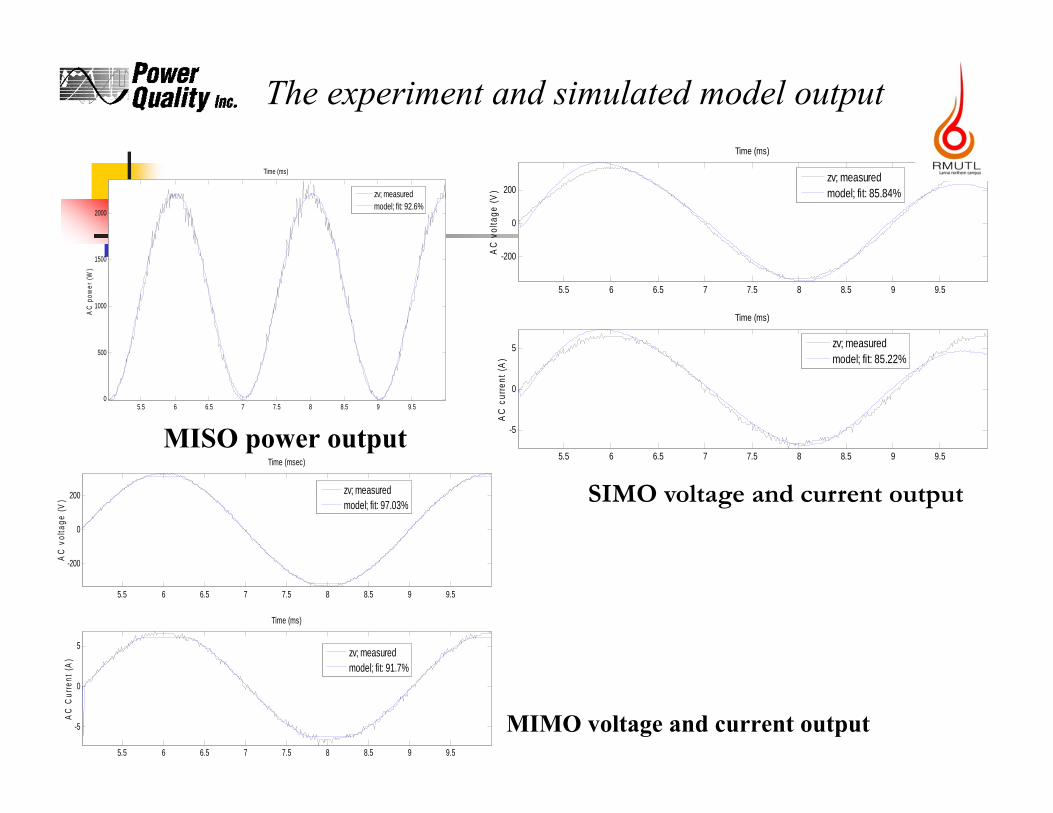
The experiment and simulated model output
5.5 6 6.5 7 7.5 8 8.5 9 9.5
-200
0
200
Time (ms)
AC
vol
tage
(V)
zv; measuredmodel; fit: 85.84%
5.5 6 6.5 7 7.5 8 8.5 9 9.5
-5
0
5
Time (ms)
AC
cur
rent
(A)
zv; measuredmodel; fit: 85.22%
5.5 6 6.5 7 7.5 8 8.5 9 9.5
-200
0
200
Time (msec)
AC
vol
tage
(V)
zv; measuredmodel; fit: 97.03%
5.5 6 6.5 7 7.5 8 8.5 9 9.5
-5
0
5
Time (ms)
AC
Cur
rent
(A)
zv; measuredmodel; fit: 91.7%
SIMO voltage and current output
MIMO voltage and current output
5.5 6 6.5 7 7.5 8 8.5 9 9.50
500
1000
1500
2000
Time (ms)
AC
pow
er (W
)
zv; measuredmodel; fit: 92.6%
MISO power output
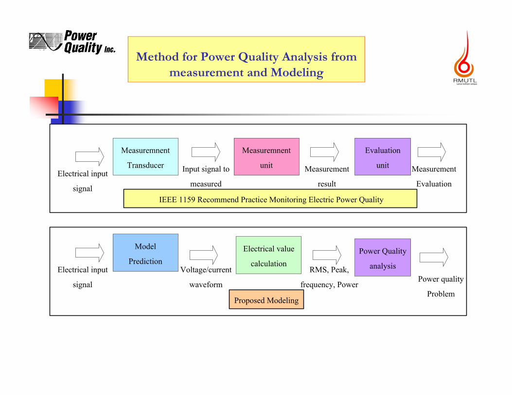
Method for Power Quality Analysis from measurement and Modeling
Measuremnent
Transducer
Measuremnent
unit
Evaluation
unitInput signal to
measured
Measurement
resultElectrical input
signal
Measurement
Evaluation
Model
PredictionElectrical input
signal
Voltage/current
waveform
Electrical value
calculationRMS, Peak,
frequency, Power
Power Quality
analysisPower quality
ProblemProposed Modeling
IEEE 1159 Recommend Practice Monitoring Electric Power Quality
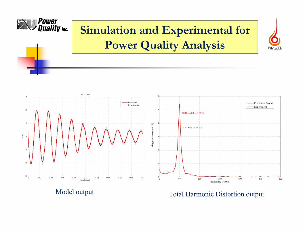
Simulation and Experimental for Power Quality Analysis
0 50 100 150 200 250 3000
1
2
3
4
5
6
Mag
nitu
de c
urre
nt (A
)
THDexp is 3.53 %
THDmodel is 3.68 %
Frequency (Hertz)
Prediction ModelExperiment
0 0.02 0.04 0.06 0.08 0.1 0.12 0.14 0.16 0.18 0.2-15
-10
-5
0
5
10
15AC current
Iac
A)
time(msec)
Prediction Experimental
Model output Total Harmonic Distortion output
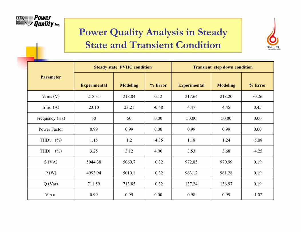
Power Quality Analysis in Steady State and Transient Condition
Parameter
Steady state FVHC condition Transient step down condition
Experimental Modeling % Error Experimental Modeling % Error
Vrms (V) 218.31 218.04 0.12 217.64 218.20 -0.26
Irms (A) 23.10 23.21 -0.48 4.47 4.45 0.45
Frequency (Hz) 50 50 0.00 50.00 50.00 0.00
Power Factor 0.99 0.99 0.00 0.99 0.99 0.00
THDv (%) 1.15 1.2 -4.35 1.18 1.24 -5.08
THDi (%) 3.25 3.12 4.00 3.53 3.68 -4.25
S (VA) 5044.38 5060.7 -0.32 972.85 970.99 0.19
P (W) 4993.94 5010.1 -0.32 963.12 961.28 0.19
Q (Var) 711.59 713.85 -0.32 137.24 136.97 0.19
V p.u. 0.99 0.99 0.00 0.98 0.99 -1.02

Gray box system identification
Recursive system identification – Kalman filtering
Model predictive control
Model order reduction – Robust control
Power Quality Analysis from Modeling
Voltage Stability Analysis from Modeling
Load flow and penetration analysis from Modeling
Model Application and Future Research
Increase accuracy and Real time modeling
Control base on Modeling
Power Quality Issuefrom Modeling
Conclusion
A model of a PV inverter has been experimentally obtainedfrom the Nonlinear Hammerstein-Wiener method.
The model consists of three parts, static input and output parts,and dynamic middle part.
The obtained model is validated and compared with theexperimental results.
The dynamic stability behavior of the system has beenanalyzed through the linearized version of the system using afrequency response analysis.
Power Quality Analysis of output system can be done by usingmodeling and standard

PQ Synergy 2014 19 May 2012