DOWNWARD FLAME FRONT SPREAD IN THIN SOLID FUELS: THEORY AND EXPERIMENTS

Bruna Comas Hervada

Dipòsit legal: Gi. 1451-2014 http://hdl.handle.net/10803/276957

http://creativecommons.org/licenses/by-nc-sa/4.0/deed.ca Aquesta obra està subjecta a una llicència Creative Commons Reconeixement-NoComercial-CompartirIgual Esta obra está bajo una licencia Creative Commons Reconocimiento-NoComercial-CompartirIgual This work is licensed under a Creative Commons Attribution-NonCommercial-ShareAlike licence

Universitat de Girona

Doctoral Thesis

Downward flame front spread inthin solid fuels: Theory and

experiments

Bruna Comas Hervada

2014

Doctoral Thesis

Downward flame front spread in thinsolid fuels: Theory and experiments

Bruna Comas Hervada

2014

Programa de doctorat en ciencies experimentals i sostenibilitat

Supervised by:Toni Pujol Sagaro

Presented in partial fulfilment of the requirements for a doctoral degree from theUniversity of Girona

This Ph.D. Thesis has produced a collection of published articles which are includedin the Appendix. The results section of this thesis is formed by the three original papersthat have been published in peer-reviewed journals. The impact factors of the journals arefrom the first and the second quartiles, according to the Journal Citation Reports (JCR)for the year 2012, for the subject categories Physics, Mathematical and Engineering,Multidisciplinary.

The complete reference of the papers and the impact factor of the journals are:

• B. Comas and T. Pujol. Flame front speed and onset of instability in the burningof inclined thin solid fuel samples. Physical Review E, 88: 063019, 2013. (ImpactFactor 2.313, journal 6 of 55, Quartile 1, category Physics, Mathematical)

• B. Comas and T. Pujol. Energy balance models of downward combustion of parallelthin solid fuels and comparison to experiments. Combustion Science and Technol-ogy, 185: 1820–1837, 2013. (Impact Factor 1.011, journal 33 of 90, Quartile 2,category Engineering, Multidisciplinary)

• B. Comas and T. Pujol. Experimental study of the effects of side-edge burning inthe downward flame spread of thin solid fuels. Combustion Science and Technology,184: 489-504, 2012. (Impact Factor 1.011, journal 33 of 90, Quartile 2, categoryEngineering, Multidisciplinary)

i

Nomenclature

Letters

a Absorptivity of paper (-)Ag Combustion preexponential term (m3kg−1s−1)As Pyrolysis preexponential term (s−1)b constant to express the convective heat flux in Chap. 3.2 (W m−2)Bc Mass transfer number (-)c Specific heat (J kg−1 K−1)C Separation between papers (cm)d Function of θs (-)D Mass diffusivity (m2 s−1)Da Damkohler number (-)Eg Combustion activation energy term (kJ mol−1)Es Pyrolysis activation energy term (kJ mol−1)f Air to fuel mass ratio (-)Fa→b View factor from surface a to surface b (-)F Factor in Eq. (3.24) (-)g Gravity (m s−2)Gr Grashof number (-)Hvap Latent heat of vaporization (J kg−1)Hcom Heat of combustion (J kg−1)Hpyr Heat of pyrolysis (J kg−1)J Heat flux in Chap. 3.3 (W m−2)L Length (mm)m′′ Mass flux of volatiles (kg m−2 s−1)N Number of papers (-)Nu Nusselt number (-)Pr Prandtl number (-)q Heat flux (W m−2)Q Heat transfer rate per unit width (W m−1)

Q′′′s−g Volumetric rate of heat transfer from the solid to the gas phase (Wm−3)

P Pressure (Pa)

iii

r Stoichiometric oxidizer to fuel mass ratio (-) in Chap. 3.2 /Correlationcoefficient in Chaps. 2 and 3.1 (-)

R Universal gas constant (8.314 J K−1 mol−1)Sc Schmidt number (-)T Temperature (K)u x-component of gas phase velocity (m s−1)v y-component of gas phase velocity (m s−1)vw Blowing velocity of volatiles from the solid (m s−1)Vf Downward flame spread velocity (cm s−1)w Sample width (mm) / z-component of gas phase velocity in Chap. 1

(m s−1)x Direction parallel to sample surface (m)X Molar fraction (-)y Direction normal to sample surface (m)Y Mass fraction (-)z Direction parallel to sample surface and parallel to flame front (m)

Greek Symbols

α Thermal diffusivity (m2 s−1)β Angle between the flame plane and the paper plane in Chap. 3.3

(deg) / Heating rate in Chap. 2 (K min−1)δ Constant to express the convective flux in Chap. 3.2 (m) / Thickness

of the boundary layer in Chap. 3.3 (m)δi Length scale (m)ε Emissivity (-)ζ Integral variable (m)η Integral variable (m)θ Flame inclination angle (deg)θs Dimensionless solid temperature, θs = (Ts − T∞)/(Tv − T∞) (-)λ Thermal conductivity (W m−1 K−1)µ Viscosity (Pa s)ν Kinematic viscosity (m2 s−1)ξ Integral variable (m)ρi Density (kg m−3)σ Stefan-Boltzmann constant (W m−2 K−4)τ Thickness (mm)φ Sample inclination angle (deg)ω′′′ Reaction term (kg m−3 s−1)

iv

Subscripts

+ From the upper side− From the lower side1 First approximation2 Second approximation∞ Ambientacv Convective (velocity)ad Adiabatic (adiabatic temperature of flame)com Combustionc Convectivede Ris Related to de Ris’ formuladx Differential strip of the sampled Downwarde Emberf Flameg Gash From paper to flamei Dummy indexj Dummy indexk Dummy indexl Dummy indexn Normal to flame frontN For N papers (if nothing stated, it refers to 1 paper)p Paperr Radiativeref Reference for calculating gas phase propertiesri Radiative from i = f1 local flame, i = f2 nearby flame, i = s surface

(losses), i = p nearby paper surface, i = e nearby embers Solidt Totalthin Thin solidsthick Thick solidsv vaporization

v

List of Figures

1.1 Schema of the downward flame spread in a vertical thin solid fuel (sym-metry along the x-axis). . . . . . . . . . . . . . . . . . . . . . . . . . . . . 11

1.2 Solid density, solid temperature and mass flux of volatiles released by thesolid. . . . . . . . . . . . . . . . . . . . . . . . . . . . . . . . . . . . . . . . 12

1.3 Density (kg m−3) contours in the gas phase at the conditions shown inFigure 1.2. . . . . . . . . . . . . . . . . . . . . . . . . . . . . . . . . . . . . 12

1.4 Temperature (K) contours and velocity vectors in the gas phase at theconditions shown in Figure 1.2. . . . . . . . . . . . . . . . . . . . . . . . . 13

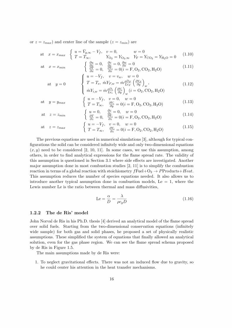
1.5 Schema of the downward flame spread in a thin solid fuel used in de Ris’model. . . . . . . . . . . . . . . . . . . . . . . . . . . . . . . . . . . . . . . 17

2.1 Schema of the experimental setup. . . . . . . . . . . . . . . . . . . . . . . 22

2.2 Specific heat curve of the cellulose sheets. . . . . . . . . . . . . . . . . . . 23

2.3 Mass fraction and derivative of the mass fraction obtained by means ofthermogravimetric analysis. . . . . . . . . . . . . . . . . . . . . . . . . . . 23

2.4 Image from one experiment. . . . . . . . . . . . . . . . . . . . . . . . . . . 24

2.5 Flame position vs. time and linear regression of a test. . . . . . . . . . . . 25

3.1 Schema of the experimental setup. . . . . . . . . . . . . . . . . . . . . . . 30

3.2 Image from one experiment . . . . . . . . . . . . . . . . . . . . . . . . . . 32

3.3 Downward flame spread rates for samples with different widths and half-thickness of 0.0933 mm in an atmosphere with XO2 = 25%. . . . . . . . . 33

3.4 Downward flame spread rates for samples of 4 cm width, with one edgeuninhibited and with both edges inhibited as a function of oxygen molarconcentration XO2 . . . . . . . . . . . . . . . . . . . . . . . . . . . . . . . . 34

3.5 Angles of the pyrolysis front with respect to the vertical side for sampleswith half-thickness of 0.0933 mm and different widths. . . . . . . . . . . . 35

3.6 Downward flame spread rates for samples with different thicknesses and awidth of 4 cm in an atmosphere with XO2 = 22%. . . . . . . . . . . . . . 36

3.7 Downward flame spread rates for samples with different edge conditions,all with a width of 4 cm in an atmosphere with XO2 = 40%. . . . . . . . . 37

3.8 Ratio of the velocity normal to the flame front in free edge experimentsVf,n and the downward flame front speed Vf . . . . . . . . . . . . . . . . . 38

3.9 Solid and gas phase control volumes at the flame leading edge. . . . . . . 40

vii

3.10 Ratio of the downward flame spread rate Vf,d in the free edge and theflame front speed Vf when both edges are inhibited as a function of theoxygen concentration. . . . . . . . . . . . . . . . . . . . . . . . . . . . . . 41

3.11 Schematic view of the experimental setup . . . . . . . . . . . . . . . . . . 453.12 Image of one experiment. . . . . . . . . . . . . . . . . . . . . . . . . . . . 463.13 Heat fluxes received on an element of the preheated zone of the paper. . . 473.14 Downward burning rate Vf as a function of the oxygen molar fraction XO2

for a single sheet. . . . . . . . . . . . . . . . . . . . . . . . . . . . . . . . . 513.15 As in Figure 3.14 but for a two parallel sheets case with a separation

distance C = 25 mm. . . . . . . . . . . . . . . . . . . . . . . . . . . . . . . 523.16 Downward burning rate Vf contours (cm/s) as a function of the ratio

between the flame temperature Tf and the adiabatic flame temperatureTf,ad, and of the oxygen molar fraction XO2 . . . . . . . . . . . . . . . . . . 53

3.17 Downward burning rate Vf as a function of the separation distance Cbetween two parallel sheets at XO2 = 30%. . . . . . . . . . . . . . . . . . 53

3.18 As in Figure 3.17 but for the I-G model only and at different oxygen molarfractions (in %). . . . . . . . . . . . . . . . . . . . . . . . . . . . . . . . . 54

3.19 As in Figure 3.17 but for cellulosic-type samples as in Kurosaki et al. [51]. 553.20 Downward burning rate Vf as a function of the separation distance C

between two parallel sheets at XO2 = 30% for different number of parallelsamples. . . . . . . . . . . . . . . . . . . . . . . . . . . . . . . . . . . . . . 56

3.21 View factor of surface S1 to a differential strip dx (K, I, and I-G models). 573.22 View factor of surface S1 to a surface S2 (A model). . . . . . . . . . . . . 583.23 Schema of the combustion chamber. . . . . . . . . . . . . . . . . . . . . . 603.24 Image from one experiment. . . . . . . . . . . . . . . . . . . . . . . . . . . 613.25 Flame spread rate versus angle to vertical of the samples. . . . . . . . . . 673.26 Normalized values of flame front speed as a function of Damkohler number. 673.27 Nu2/Nu1 for all XO2 tested, experimental results and expected curves. . . 69

4.1 Heat fluxes received at the unburned sample simulated with the modelemployed in Section 3.2. . . . . . . . . . . . . . . . . . . . . . . . . . . . . 77

viii

List of Tables

3.1 Summary of previous works that obtain data related to the downwardcombustion of solid fuels with free edges at absolute pressure P = 105 Pa(or similar), normal gravity and initially quiescent environment. . . . . . . 28

4.1 Summary of previous works that obtain data related to the downwardcombustion of solid fuels with free edges at an absolute pressure of P =105 Pa (or atmospheric pressure), normal gravity and initially quiescentenvironment. We include the work done in Section 3.1. Same as Tab. 3.1. 72

4.2 Summary of previous works that obtain data related to the downwardcombustion of solid fuels with more than one sample at an absolute pres-sure of P = 105 Pa (or atmospheric pressure), normal gravity and initiallyquiescent environment. We include the work carried out in Section 3.2. . . 73

4.3 Summary of previous works that obtain data related to inclined downwardcombustion of solid fuels at an absolute pressure of P = 105 Pa (or atmo-spheric pressure), normal gravity and initially quiescent environment. Weinclude the work carried out in Section 3.3. . . . . . . . . . . . . . . . . . 74

ix

El Dr. Toni Pujol i Sagaro, de la Universitat de Girona,

DECLAROQue el treball titulat Downward flame front spread in thin solid fuels: Theory and expe-riments, que presenta Bruna Comas i Hervada per a l’obtencio del tıtol de doctora, haestat realitzat sota la meva direccio i que compleix els requisits per poder optar a MencioInternacional.

I, perque aixı consti i tingui els efectes oportuns, signo aquest document.

Signatura

Girona, 26 de maig de 2014.

xi

To my wife and daughter

xiii

Acnowledgements

First of all I would like to thank Dr. Toni Pujol for providing the opportunity to conductthis research, he has made a lot of suggestions during these years and has become theprincipal support of this thesis. This adventure also started under the supervision of Dr.Quim Fort, and would have been impossible to start without him.

I want also to thank my supervisor in Lund University, Dr. Patrick van Hees, for hisguidance during my stay there and for having let me conduct some experiments.

This thesis has been possible thanks to FPU (Formacion de Profesorado Universitario)fellowship program funded by Ministerio de Educacion, Cultura y Deporte.

I wish to extend my gratitude to all my friends and colleagues from Universitat deGirona, the ones from my former department, the Physics Department, and from mynew department, the Mechanical Engineering and Industrial Construction department.Specially to my fellow Ph.D. students and my office colleague for the friendship and goodtimes.

I appreciate the friendship and hospitality of the Marie Curie Ph.D. students fromLund University. My stay there wouldn’t have been the same without them.

Last but not least, I would like to thank my family for their enormous support andencouragement. This thesis wouldn’t have been possible without them. They were thesource for my motivation. In particular, my wife Marta and my daughter Lia.

xv

Contents

Nomenclature iii

List of Figures viii

List of Tables ix

Acknowledgements xv

Resum 3

Resumen 5

Abstract 7

1 Introduction 91.1 The flame spread problem . . . . . . . . . . . . . . . . . . . . . . . . . . . 101.2 Theory and models . . . . . . . . . . . . . . . . . . . . . . . . . . . . . . . 131.3 Objectives . . . . . . . . . . . . . . . . . . . . . . . . . . . . . . . . . . . . 20

2 Methodology 212.1 Experimental Setup . . . . . . . . . . . . . . . . . . . . . . . . . . . . . . 212.2 Samples . . . . . . . . . . . . . . . . . . . . . . . . . . . . . . . . . . . . . 212.3 Experimental procedure . . . . . . . . . . . . . . . . . . . . . . . . . . . . 24

3 Results 273.1 Experimental study of the effects of side-edge burning in the downward

flame spread of thin solid fuels . . . . . . . . . . . . . . . . . . . . . . . . 273.2 Energy Balance Models of Downward Combustion of Parallel Thin Solid

Fuels and Comparison to Experiments . . . . . . . . . . . . . . . . . . . . 433.3 Flame front speed and onset of instability in the burning of inclined thin

solid fuel samples . . . . . . . . . . . . . . . . . . . . . . . . . . . . . . . 59

4 Discussion 714.1 Comparison with previous studies . . . . . . . . . . . . . . . . . . . . . . . 714.2 Experimental results . . . . . . . . . . . . . . . . . . . . . . . . . . . . . . 73

1

4.3 Theoretical models . . . . . . . . . . . . . . . . . . . . . . . . . . . . . . . 75

5 General conclusions 79

Bibliography 83

A Publications 89Combustion Science and Technology, 184: 489–504, 2012 . . . . . . . . . . . . . 89Combustion Science and Technology, 185: 1820–1837, 2013 . . . . . . . . . . . 106Physical Review E, 88: 063019, 2013 . . . . . . . . . . . . . . . . . . . . . . . . 124

2

Resum

La propagacio de flames en solids es un fenomen complex que inclou processos que passena la fase solida i a la fase gasosa. Diversos autors han estudiat aquest fenomen des dediferents punts de vista ja que es un element clau en l’analisi del risc d’incendis i dedinamica de focs. En aquesta tesi doctoral estudiem la propagacio de flames en solidsprims en processos mes complexos que els processos classics, on la flama es propaga avallen una mostra vertical o horitzontal.

El Capıtol 1 descriu el problema de la propagacio de la flama cap avall i dirimeixclarament els objectius del treball. La metodologia aplicada per a obtenir les dadesexperimentals es descriu al Capıtol 2.

El Capıtol 3 es compon de tres seccions que son el nucli d’aquesta tesi. La Seccio 3.1fa un estudi complet del metode experimental i estableix el procediment per a fer provesacurades. Tambe mesura la influencia de les vores tot usant diferents tipus de suports demostra i tot cremant mostres amb un costat sense agafar (amb i sense parets gruixudesproperes). Les dades experimentals s’obtenen a fraccions molars d’oxigen diferents i ambmostres de diferents gruixos. A mes es deriva un model simple per a la velocitat depropagacio del front de flama, que s’ha d’entendre com a una extensio de la formulaclassica de de Ris.

La seguent seccio, la Seccio 3.2 estudia l’efecte de la combustio vertical d’un conjuntde mostres paral·leles. Les dades experimentals s’obtenen en funcio de la fraccio molard’oxigen i de la separacio entre mostres. En aquest capıtol generalitzem un model debalanc d’energia detallat que inclou fluxos de calor radiatius per tal que sigui completa-ment predictiu. En aquesta seccio tambe derivem un model analıtic senzill que es unageneralitzacio del model de de Ris, i que inclou explıcitament els efectes radiatius. Aquestmodel reprodueix raonablement be les velocitats observades.

La Seccio 3.3 explora experimentalment i teoricament la propagacio cap avall de laflama en mostres inclinades. Es centra en la inestabilitat convectiva que apareix enmostres inclinades que cremen en angles propers a la horitzontal, i proposa una novametodologia per predir l’angle crıtic a partir del qual apareix aquesta inestabilitat. Lavalidesa del nostre metode, basat en el nombre de Nusselt, es confirmada experimental-ment amb dades obtingudes a diverses concentracions ambientals d’oxigen.

3

Resumen

La propagacion de llamas en solidos es un fenomeno complejo que incluye procesos queocurren en la fase solida y gaseosa. Diversos autores han estudiado este fenomeno desdedistintos puntos de vista, ya que es un elemento clave en el analisis del riesgo de incendiosy de dinamica del fuego. En esta tesis doctoral estudiamos la propagacion de llamas ensolidos con reducido grosor en procesos mas complejos que los procesos clasicos, dondela llama se propaga hacia abajo en una muestra vertical o horizontal.

El Capıtulo 1 describe el problema de la propagacion de llama hacia abajo y dirimeclaramente los objetivos del trabajo. La metodologıa aplicada para obtener los datosexperimentales se describe en el Capıtulo 2.

El Capıtulo 3 se compone de tres secciones que son el nucleo de esta tesis. La Seccion3.1 hace un estudio completo del metodo experimental y establece el procedimiento parahacer experimentos precisos. Tambien mide la influencia de los lados usando distintostipos de soportes para la muestra y quemando muestras con un lateral libre (con y sinparedes laterales gruesas). Los datos experimentales se obtienen para fracciones molaresde oxıgeno distintas y con muestras de distinto grosor. Ademas se deriva un modelosimple para la velocidad de propagacion de la llama, que se debe entender como unaextension de la formula clasica de de Ris.

En la siguiente seccion, la Seccion 3.2, se estudia el efecto de la combustion vertical deun conjunto de muestras paralelas. Los datos experimentales se obtienen en funcion de lafraccion molar de oxıgeno y de la separacion entre muestras. En esta seccion se generalizaun modelo de balance de energıas detallado que incluye flujos de calor radiativos para quesea completamente predictivo. Tambien se deriva un modelo analıtico simple que es unageneralizacion del modelo de de Ris y que incluye explıcitamente los efectos radiativos.Este modelo reproduce razonablemente bien las velocidades observadas.

La Seccion 3.3 explora experimentalmente y teoricamente la propagacion de la llamahacia abajo en muestras inclinadas. Se centra en la inestabilidad convectiva que apareceen muestras cuyo angulo de inclinacion es proximo a la horizontal, y propone una nuevametodologıa para predecir el angulo crıtico a partir del cual la inestabilidad aparece. Lavalidez de nuestro metodo, basado en el numero de Nusselt, es confirmada experimental-mente con datos obtenidos en concentraciones ambientales de oxıgeno distintas.

5

Abstract

Flame spread over solid samples has been studied from many points of view, as it is keyfor fire safety, yet it is a complex phenomenon that involves processes occurring in boththe solid and the gas phases. In the present Ph.D. thesis we study flame spread over thinsolid samples in processes more complex than the classical cases where a flame spreadsdownward over a vertical solid sample or horizontally.

Chapter 1 describes the downward flame spread problem and clearly states the ob-jectives of our work. The methodology applied for obtaining the experimental data isdetailed in Chapter 2.

Chapter 3 includes the three sections that are the core of this thesis. Section 3.1 makesa thorough study of the experimental method and establishes a procedure for accuratelymaking tests. It also measures the influence of the side effects by using different types ofsample holders and by burning the sample with one free edge (with and without nearbysidewalls). The experimental data is obtained at different oxygen molar fractions andwith samples of different thickness. A simple model of the flame front speed, that may beunderstood as an extension of the classical de Ris’ formula for thin solid fuels, is derived,acting as a reasonable upper bound of the data we have obtained.

The next section, Section 3.2, shows the effects of a downward combustion of anarray of parallel samples. Experimental data are obtained as a function of the oxygenmolar fraction and the separation distance between parallel samples. In this chapter wegeneralize a detailed energy balance model that includes radiative heat transfer in orderto be fully predictive. Also in this section, a simple analytical model of the flame frontspeed is derived, which is a generalization of the de Ris’ formula by explicitly includingthe radiative effects. The models remarkably reproduce the observed data.

Section 3.3 explores the inclined (downward) burning of thin solid samples, bothexperimentally and theoretically. It focuses on the convective instability that arises whensamples are burning almost horizontally, and proposes a new methodology to predict thecritical angle at which arises the onset of the instability. The validity of our method,based on the Nusselt number, is experimentally confirmed with data obtained at differentoxygen concentrations of the environment.

7

Chapter 1

Introduction

Flame spread over solid samples is a complex process of great importance from the pointof view of fire safety. In addition, it is key for understanding the fundamentals of combus-tion processes involving pyrolysing materials. Here we restrict our study to downwardcombustion of thermally thin solids. The latter condition applies to a sample with athickness smaller than its characteristic thermal length1. In the literature, theoretical aswell as experimental methods are used for determining the propagation speed of the flamefront when burning thin solid fuels. The usual theoretical approach consists of startingfrom the comprehensive conservation equations and then simplify them after applyingsome argumented assumptions. The result is either an analytical expression or a setof partial differential equations that form the core of a numerical model whose solutionallows us to obtain the flame spread rate. On the other hand, experimental data areusually collected by using a combustion chamber with a given atmospheric concentrationand burning a vertical cellulosic-type sample from the top.

This Ph.D. thesis aims to contribute to the knowledge of the downward combustionof thin solid fuels by analysing this phenomenon in more complex situations than thoseusually applied in common studies (vertical downward combustion with the sample heldby both lateral edges). The results obtained in this Ph.D. thesis haven been publishedin peer-reviewed journals. The results section, Section 3, consists of a transcription ofthese articles organized in three sections. Section 3.1 experimentally studies the effectof having a free lateral edge on the flame front speed and it develops a simple analyticalexpression that can be understood as an upper bound of the flame spread rate. ThenSection 3.2 generalizes a classical energy balance model in order to include radiativeeffects and to explain the flame front speed when multiple parallel thin solid sheets areburnt downwards. These sections are focused on vertical burning. In this configuration,convection induces an upward flow parallel to the sample surface and opposed to the flamefront velocity. However, in the downward burning of an inclined sample, backgroundflow instabilites arise beyond a critical angle of inclination due to the change of gravityorientation with respect to the sample surface. Section 3.3 investigates this effect andproposes a methodology valid for different atmospheric conditions for predicting such a

1δgx = αg/(Vf + Vg); see the nomenclature section for the definition of symbols and variables.

9

critical angle of inclination.

1.1 The flame spread problem

The flame spread process over solid fuels is described in two steps: first of all there is anendothermic reaction named pyrolysis that takes place in the solid phase. This reactiondegrades the solid that produces gases (pyrolysate). After that a strongly exothermicreaction named combustion occurs in the gas phase. There, ambient oxygen and fuelvolatiles of the pyrolysate combine to form products and release heat that produces avisible flame. This mechanism starts with an external heat source that pyrolyses thesolid until the quantity of fuel volatiles is sufficient to produce a flame. It is sustained bythe heat fluxes produced in the combustion process that preheat the virgin solid aheadof the flame front. In Figure 1.1 we can see the schema of the downward flame spreadover a thin solid fuel. Only half is depicted, as it is symmetrical with respect to the halfthickness of the solid in the vertical burning case.

Besides the articles reproduced in this text, over the course of this Ph.D. we have alsodeveloped a transient fully-coupled two-dimensional numerical model of the downwardflame spread process. For thin solid fuels and neglecting radiative effects, preliminaryresults of these simulations allow us to obtain the expected profiles in the gas phase aswell as in the solid phase when burning a cellulosic paper with half-thickness τ/2 = 0.0933mm and density ρs = 461.95 kg m−3 in an environment with no forced flow and oxygenmolar fraction XO2 = 0.23.

In Figure 1.2 we can see the solid density and temperature, coupled with the flux ofvolatiles released by the solid. In the case shown, the flame is propagating to the left(downwards) with the leading edge of the pyrolysis front at 0.003 m approximately. Notethe degradation of the solid in the region where pyrolysis exists, with a solid densitydecreasing to a minimum value (char density) whereas it is almost constant and equal tothe virgin value ahead of the front. The volatiles (non-zero values of the mass flux) arereleased in this pyrolysing region. Also in this region, the solid temperature reaches analmost constant value, whereas there exists a preheating zone with no solid degradationahead of the front. This behaviour is very similar to that obtained in Refs. [1, 2], beingcommon to all processes of downward flame spread in thin solid fuels.

The next two figures show the characteristic behaviour of the main physical variablesin the gas phase. Figure 1.3 displays the fluid density contours in the gas phase atthe same time that occurs Figure 1.2 in the solid one. These density variations aredue to changes in temperature and induce an opposed buoyancy-driven flow since thepropagation is downwards (towards negative x values). Simulations reveal, as in Figure1.4, that the flame front may be located slightly ahead of the pyrolysis front and that itdoes not touch the surface. We point out that Figures 1.2-1.4 have been obtained aftersolving a preliminary version of a numerical model based on the finite volume method.Therefore, the results are solely shown for a qualitative understanding of the flame spreadproblem. More work is needed for obtaining accurate solutions, especially more effort isrequired for adequately defining the boundary conditions of the computational domain.

10

Figure 1.1: Schema of the downward flame spread in a vertical thin solid fuel (symmetryalong the x-axis).

11

0.000 0.002 0.0040

100

200

300

400

500

600

700

Solid density

Den

sity

(kg

m-3)

Sample length (cm)

0.00

0.05

0.10

0.15

Mass flux of volatiles

Mas

s flu

x (k

g m

-2 s

-1)

300

400

500

600

700

Solid temperature

Tem

pera

ture

(

Figure 1.2: Solid density, solid temperature and mass flux of volatiles released by thesolid.

Figure 1.3: Density (kg m−3) contours in the gas phase at the conditions shown inFigure 1.2.

12

Figure 1.4: Temperature (K) contours and velocity vectors in the gas phase at theconditions shown in Figure 1.2.

1.2 Theory and models

In this section we introduce the comprehensive three-dimensional governing equations forthe gas phase reaction (combustion) and the one-dimensional governing equations for thesolid phase reaction (pyrolysis) that take place in the flame spread over a thin solid fuel.These equations are used in complex numerical simulations [3]. Under some reasonableassumptions applied to these equations, we may reach analytical expressions for the flamefront speed. We then describe the model proposed by de Ris in his Ph.D. thesis [4], whichwas the first physically-based model that obtained an analytical expression for the flamespread rate based on a simplified version of a two-dimensional model. As stated in thereview of the flame spread process over solid fuels written by Wichman [5], the discussionof the physical processes involved in the combustion of solid fuels made in de Ris’ Ph.D.thesis is still valid and it becomes a crucial contribution to the field of flame spread.

1.2.1 Governing equations

The pyrolysis process in the solid phase can be described in multiple ways, depending onthe material that burns and the degree of complexity wanted. In this thesis we use theword pyrolysis meaning a generic reaction that releases gases from a solid, as it is usedin the fire research community, nor as it is used in chemical engineering as the anaerobicthermal degradation of solids. We assume that cellulosic materials are charring materialsand that melting, bubbling and shrinkage/swelling of the solid can be neglected. Thesimplest way to model the pyrolysis reaction is using an ablation model that defines apyrolysis temperature Tv where the reaction takes place. The solid temperature is lowerthan Tv in the region with no reaction. This model implicitly considers that the pyrolysis

13

reaction is controlled by heat transfer and that the kinetics of the reaction is infinite [6].By using this model, pyrolysis is defined with two parameters: the pyrolysis temperatureTv and the heat of pyrolysis Hpyr.

The next degree of complexity is to introduce finite-rate kinetics using a one-stepArrhenius reaction term, ω′′′fg = ρsAsexp [−Es/(RTs)] (the subscript fg denotes the re-action term from fuel to gas). This was first introduced by Kung [7] for wood pyrolysis.By using finite-rate kinetics, we allow the pyrolysis reaction to happen not only at thesurface but throughout the thickness of the solid. This effect is very important in ther-mally thick solids [3, 6, 8]. Pyrolysis models are reviewed thoroughly in Refs. [6, 9], thisnot being the objective of this thesis. We suppose that all the fuel burns out and thereis no char left. The local mass flux from the solid to the gas phase can be written as

m′′(z) =

∫ z

δω′′′fgdζ = −ρvw(z) (1.1)

in the flame front fixed coordinates, with vw the blowing velocity of the fuel to theambient, which depends on the gas density and the thickness of the solid [3, 6]. The localenergy conservation is

ρscs∂T

∂t+ ρscsvw

∂T

∂z= −~∇ · ~Js − ω′′′fg∇Hpyr − Q′′′s−g + q′′′r (1.2)

where Q′′′s−g is the volumetric rate of heat transfer from the solid phase to the gas one.

By assuming thermal equilibrium between both phases we find Q′′′s−g = m′′cg∂Tg∂z . In

Eq. (1.2) ~Js comprises both radiative and convective heat fluxes. This model is one-dimensional, ignores conductive heat fluxes to other parts of the solid and supposes thatall the volatiles generated escape instantaneously [6]. A detailed model of the radiativeheat flux can be seen in Bhattacarjee et al.’s work [10] who use a similar model appliedto a surface solid element.

On the other hand, the comprehensive gas phase governing equations can be expressedas [3]

• Continuity∂ρ

∂t+∇ ·

(ρ ~Vg

)= 0 (1.3)

• x -momentum

∂ (ρu)

∂t+∇ ·

(ρu ~Vg − µ∇u

)= −∂ (p− p∞)

∂x+

{∂

∂x

[1

3µ∂u

∂x−

−2

3µ

(∂v

∂y+∂w

∂z

)]+

∂

∂y

[µ∂v

∂x

]+

∂

∂z

[µ∂w

∂x

]}+ g (ρ∞ − ρ)

(1.4)

with z the coordinate along the width of the sample and x positive in the directionopposite to the propagation.

14

• y-momentum

∂ (ρy)

∂t+∇ ·

[ρv ~Vg − µ∇v

]= −∂ (p− p∞)

∂y+

{∂

∂x

[µ∂u

∂y

]+

∂

∂y

[1

3µ∂v

∂y− 2

3µ

(∂u

∂x+∂w

∂z

)]+

∂

∂z

[µ∂w

∂y

]} (1.5)

• z -momentum

∂ (ρw)

∂t+∇ ·

[ρw ~Vg −∇w

]= −∂ (p− p∞)

∂z+

{∂

∂x

[µ∂u

∂z

]+

∂

∂y

[µ∂v

∂z

]+

∂

∂z

[1

3µ∂w

∂z− 2

3µ

(∂u

∂x+∂v

∂y

)]} (1.6)

• Species equation

∂ (ρYi)

∂t+∇ ·

(ρYi ~Vg − ρDi∇Yi

)= ω′′′i (1.7)

for i = F, O2, CO2, H2O, N2. The source (or sink) term for species i is

ω′′′i = fiω′′′F = fiAgρ

2YFYOexp

(−EgRT

)(1.8)

Considering that the fuel is cellulose, the stoichiometric combustion can be writtenas C6H10O5+6(O2+3.76N2)→ 6CO2+5H2O+22.56N2, so that the stoichiometricratios are fF = −1, fO2 = −1.1852, fCO2 = 1.6296, fH2O = 0.5556 and fN2 = 3.901.

• Energy equation

∂ (ρcgT )

∂t+ cg∇ ·

[ρT ~Vg −

(λ

cg∇T)]

=

N∑i=1

ρDicp,i (∇Yi · ∇T )−N∑i=1

ω′′′i hi +∇cg · ∇T(λ

cg

) (1.9)

with cg the weighted specific heat.

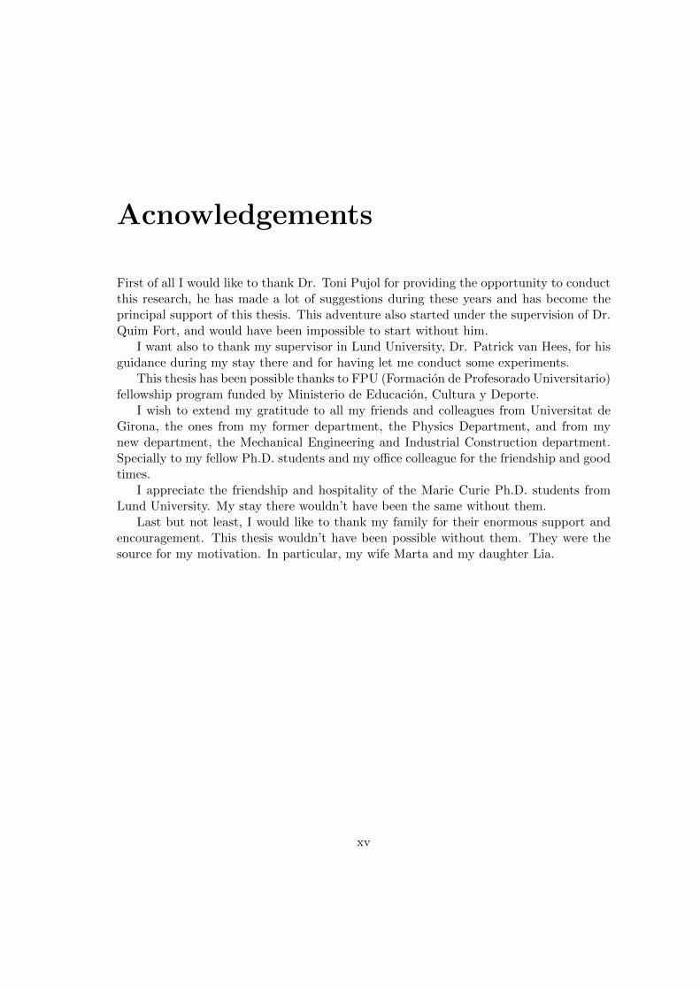
The most common boundary equations for combustion within an enclosure at down-stream (x = xmin), upstream (x = xmax), fuel surface (y = 0), chamber walls (y = ymax

15

or z = zmax) and center line of the sample (z = zmin) are

at x = xmax

{u = Vg,∞ − Vf , v = 0, w = 0T = T∞, YO2 = YO2,∞ YF = YCO2 = YH2O = 0

(1.10)

at x = xmin

{∂u∂x = 0, ∂v

∂x = 0, ∂w∂x = 0∂T∂x = 0, ∂Yi

∂x = 0(i = F,O2,CO2,H2O)(1.11)

at y = 0

u = −Vf , v = vw, w = 0

T = Ts, mYF,w = mρDFLeF

(∂YF∂y

)w,

mYi,w = mρDi

Lei

(∂Yi∂y

)w

(i = O2,CO2,H2O)

(1.12)

at y = ymax

{u = −Vf , v = 0, w = 0

T = T∞,∂Yi∂y = 0(i = F,O2,CO2,H2O)

(1.13)

at z = zmin

{u = 0, ∂v

∂z = 0, w = 0∂T∂z = 0, ∂Yi

∂z = 0(i = F,O2,CO2,H2O)(1.14)

at z = zmax

{u = −Vf , v = 0, w = 0

T = T∞,∂Yi∂z = 0(i = F,O2,CO2,H2O)

(1.15)

The previous equations are used in numerical simulations [3], although for typical con-figurations the solid can be considered infinitely wide and only two-dimensional equations(x, y) need to be considered [2, 10, 11]. In some cases, we use this assumption, amongothers, in order to find analytical expressions for the flame spread rate. The validity ofthis assumption is questioned in Section 3.1 where side effects are investigated. Anothermajor assumption done in most combustion studies [2, 11] is to simplify the combustionreaction in terms of a global reaction with stoichiometry fFuel+O2 → PProducts+Heat.This assumption reduces the number of species equations needed. It also allows us tointroduce another typical assumption done in combustion models, Le = 1, where theLewis number Le is the ratio between thermal and mass diffusivities,

Le =α

D=

λ

ρcgD(1.16)

1.2.2 The de Ris’ model

John Norval de Ris in his Ph.D. thesis [4] derived an analytical model of the flame spreadover solid fuels. Starting from the two-dimensional conservation equations (infinitelywide sample) for both gas and solid phases, he proposed a set of physically realisticassumptions. These simplified the system of equations that finally allowed an analyticalsolution, even for the gas phase region. We can see the flame spread schema proposedby de Ris in Figure 1.5.

The main assumptions made by de Ris were:

1. To neglect gravitational effects. There was not an induced flow due to gravity, sohe could center his attention in the heat transfer mechanisms.

16

Figure 1.5: Schema of the downward flame spread in a thin solid fuel used in de Ris’model.

2. Simplification of vaporization processes (sublimation, pyrolysis, melting and evap-oration) to sublimation. Thereby solids had a constant heat of vaporisation and adefined vaporization temperature (infinite pyrolysis reaction rate).

3. Simplification of the flame structure as a simple diffusion flame (infinite combustionreaction rate). The processes in the solid phase were simplified in a way thatwhen the solid was heated and reached the vaporization temperature, it releasedgases with a given heat of vaporization. This allowed a great simplification of thegoverning equations, although it led to a higher reaction rate than the actual one.For this reason, he applied an ’ad hoc’ factor to decrease the mass flux of volatiles(ln(1 + Bc) where Bc is the Spalding, or mass transfer, Bc number [12]). He alsodiscussed the flame structure near the tip, and pointing out that it should be atriple-flame near the cold wall, the main flame front where reactants reacted instoichiometric proportions and two secondary flame fronts, one ahead of the flamefront, lean (with a higher proportion of oxygen), and one after, rich (with more fuel).After defining that, he avoided the problem by setting the ignition temperaturebelow the vaporization temperature of the solid. Thus the flame touched the coldsample surface, with no oxygen after the flame and no fuel in front. He used themodel for diffusion flames from Schvab and Zeldovich [13] that considered infinitethe chemical reaction rate, so the flame was confined in a thin sheet and fuel andoxygen were consumed at stoichiometric proportions.

4. Oseen flow approximation. The environment would move, either by an opposingflow fed by the lab design or by an induced flow due to buoyancy effects. Heconsidered this opposed flow as a laminar flow with a constant velocity Vg parallelto the fuel, thus using the Oseen flow approximation. Note that this approximationbreaks the no-slip condition at the solid surface, although it is a valid solution forthe Navier-Stokes equations.

5. Lewis number equal to unity. De Ris set the Lewis number to 1, as the air Lewis

17

number is Le ≈ 0.9. By setting it to 1, one term dropped from the equations aftercombining them. This approximation is commonly used in other studies [2, 11]and it is also used in this Ph.D. thesis. The effect of taking into account a massdiffusion by setting Le 6= 1 is to change the flame spread rate in the way pointedout in Refs. [3, 14, 15, 16].

6. To neglect radiative heat transfer. De Ris did not consider radiative heat fluxesin his main flame spread rate expressions. He discussed them supposing an ex-ponential net radiative heat flux from the gas to the solid surface, and arrived tothe conclusion that radiative effects could be accounted by reducing the heat ofcombustion or, equivalently, the effective adiabatic stoichiometric flame tempera-ture Tf,ad. Posterior studies showed that the radiative heat transfer term could beneglected in the thermal regime or, equivalently, far away from combustion limitsdue to reduced oxygen environmental contents and/or to low gravity values [17].Radiative effects are also important for various simultaneously burning samples,where the main interaction mechanism between them is the radiative heat transfer.These effects are investigated in Section 3.2 of the results chapter.

With all these assumptions, de Ris derived two formulas for the flame spread rate forboth thermally thin and thermally thick solids:

Vf,thin =π

4

λg(τ/2) csρs

(Tf,ad − Tv)(Tv − T∞)

(1.17)

Vf,thick =√

2αsτ

λsλg

√ρgcgλgρscsλs

(Tf,ad − Tv)(Tv − T∞)

(1.18)

where it is assumed that conduction effects through a thin solid sheet are negligible asthe sample has the same Ts value for the whole thickness.

The transition from thermally thin to thick fuel occurs when the solid half-thicknessτs satisfies τs ≥

√αsαg/ [(Vf + Vg)Vf ] [18], which is equivalent to say when the square of

the solid half-thickness is greater than the product of the characteristic thermal lengthsof gas δgx = αg/(Vf + Vg) and solid δsx = αs/Vf phases.

1.2.3 Energy balance models

The objective of global energy balance models is to apply the conservation of energyto the desired control volume or surface. All the heat fluxes that enter or exit thiscontrol volume have to be identified and added to the energy conservation equation.Global energy models are mainly useful for thermally thin solids, as conductive heatfluxes through the solid would make difficult to find an analytical expression for theflame spread rate in thermally thick ones.

Energy balance models are used in Sections 3.1, 3.2 and 3.3 of Chapter 3 in order toderive an expression for the flame spread rate. In Section 3.2 the control volume is aninfinitesimal length of the preheated zone of the sample (which is burning downwards).

18

The flame spread of a wide enough sample can be described as a one-dimensional phe-nomena, and for thermally thin solids the temperature of the whole thickness can beconsidered constant. As we will derive in Section 3.2, the energy balance for one elementof the preheated zone is then

λsd2Tsdx2

+ ρscsVfdTsdx

+1

τ(qc + qr) = 0 (1.19)

where the convective heat flux is due to the environmental gas flow and the radiativeheat fluxes have to be identified for every source, being usually modeled as gray-bodyemitters.

1.2.4 Experimental studies

The experimental work related with the flame spread can be done in a combustion cham-ber [19, 20], in a wind tunnel (as in the narrow channel apparatus employed in Ref.[21, 22]) or in open air [23]. The combustion chamber is a closed device that can betotally vacuumed and filled with the desired gases at the desired concentration. Dataare collected with the background flow at rest. In the wind tunnel configuration a back-ground flow of known composition and velocity flows over the sample. Wind tunnelswith very narrow channels are employed in order to suppress convection effects and tosimulate microgravity conditions (e.g., [21, 22]).

The main measurement done in these types of studies is the flame spread rate viarecordings of the pyrolysis front position at determined times, although other measure-ments can be done [24]. Temperature measurements can also be obtained by usingthermocouples placed at the desired locations or through laser interferometry [5, 25]. Aqualitative evaluation of the gas phase around the flame can be done using Schlierenphotography [26].

The materials used for these types of experiments are mainly PMMA and cellulosicsamples [5, 6]. The experiments can be done either with thermally thin or thermallythick samples. While this classification does not change substantially the experimentdone, being an ad-hoc differentation, it is used in theoretical work [27] to simplify theset of equations employed to simulate the process. In this Ph.D. thesis we use thermallythin samples.

The air flow can be forced by an external source in a wind tunnel or it can be induced(by gravity), and its direction can be opposed or concurrent to the flame propagation.Concurrent flow flame spread can be divided into three regimes regarding the samplethickness: 1) the kinetic regime, where spread rates increase with the thickness, andwhere both pyrolysis and flame lengths are short (τ < 0.4 · 10−4 m); 2) the thermallythin regime, where flame spread rates decrease as the solid thickness increases and whereboth pyrolysis and thermal lengths increase, and 3) the thermally thick regime, whereflame spread rate is constant (τ > 0.25 · 10−2 m) [24]. Opposed flow flame spread hasalso a similar classification regarding the flame thickness.

This thesis deals with opposed flow flame spread induced by buoyancy flows. Down-ward flame spread (vertical or inclined) arises after igniting the sample at the top. Short

19

after ignition the front propagation reaches a steady spread rate downward the sample.We experiment with changing thickness, width and lateral holders in Section 3.1, withthe effects of having a parallel array of samples in Section 3.2 and with the effects ofvarying the sample angle of inclination in Section 3.3.

1.3 Objectives

The aims of this thesis are to: (1) Study the flame front propagation in processes morecomplex than the classical vertically downward one and understand its behaviour; (2)Develop new analytical models that generalize the classical ones and apply them to newconditions (e.g. by including radiative effects in analytical models); (3) Go beyond thebalance energy models and explain the convective instabilities that arise in the downwardcombustion of inclined samples.

20

Chapter 2

Methodology

This Ph.D. thesis is made as a collection of articles that are included in the followingchapters. Each article briefly describes the methodology employed, which usually consistsof developing a model for deriving an expression of a key parameter involved in thecombustion process (e.g. the flame spread rate) and testing it experimentally. Modelswill be defined in detail in the following chapters. The experimental design, which iscommon for all the articles, is here explained for the sake of completeness.

2.1 Experimental Setup

Figure 2.1 shows the combustion chamber used in our experiments. It is a cylindricalgalvanized steel chamber with a volume of 0.0458 m3. It has a 29.5×10 cm width PMMAtransparent window in order to record the tests. The chamber can also be inclined atany desired angle.

Vacuum can be made inside the chamber by means of a Telstar Torricelli 2G-6 vacuumpump. We can reach an absolute pressure less than 0.25% of the external (ambient)one. Pressure values inside the chamber are measured with a Wika CPG1000 digitalmanometer. The system that supplies gases allows us to fill the chamber with oxygenO2, and a diluent at the desired partial pressures. The diluent used in this Ph.D. thesishas been nitrogen N2. Tests are done at an absolute pressure of 105 Pa, with variousconcentrations of oxygen (ranging from XO2 = 20% to 100%).

2.2 Samples

The samples used in our studies are cellulosic sheets of half-thickness τ/2 = 0.0933 mmand a density of ρs = 461.95 kg m−3. The length of the sheets used differs in each chapterof the thesis, ranging from 16 cm to 27 cm, with a typical width of 4 cm. From the studyof the side-effects carried out in Chapter 3.1, this width is a good compromise betweenbeing insensitive to side effects and not depleting an excessive amount of oxygen as thesample is burnt. We note that in any case the sample length is chosen so that the oxygendepletion inside the chamber due to the burning process is always less than 2%.

21

Figure 2.1: Schema of the experimental setup.

The physical properties of our cellulosic sheets have been investigated. The thermalconductivity λs is determined using a hot plate at 50oC with cellulose on and a PMMAplate covering it. This experiment is described in Chapter 3.1. It uses three thermocou-ples placed at the central point of the interface hot plate-cellulose, cellulose-PMMA andon top of the PMMA plate, and works under the assumption that the heat flux throughboth solids is the same. Then, using Fourier’s law and knowing the thermal conductivityof PMMA, we determine that λs = 0.101 Wm−1K−1 with a 5% of error near ambienttemperature.

The specific heat capacity cs curve for our cellulose sample is obtained by using aDifferential Scanning Calorimetry (DSC) technique, and it is shown in Figure 2.2. Itincreases from 1180 J kg−1 K−1 at 300 K to 2370 J kg−1 K−1 at 530 K. A linear fit inthis range gives cs(T ) = (6.104± 0.003)T + (954.7± 0.4) J kg−1 K−1.

We have performed a Thermogravimetric Analysis (TGA) to study the pyrolysis ofour sheets. Tests were performed at constant heating rates of β = 2, 5, 10, and 20 Kmin−1. Figure 2.3 shows the result of one test done at β = 20 K min−1. We can see thatthere are two degradation processes, one near 620 K and the other near 750 K, which iscoherent with the models and the experiments reviewed by Milosavljevic [28] for cellulose.By using an Arrhenius first-order one step model for the main solid decomposition[29], wehave analysed the main degradation process using the Kissinger method, from which wehave obtained the preexponential term As = 3.457× 1010 s−1 and the activation energyEs = 145.716 kJ mol−1.

22

350 400 450 500 550 6001000

1200

1400

1600

1800

2000

2200

2400

cp

linear fit for T range [320:500]

c p (J

kg-1

K-1)

Temperature (K)

Figure 2.2: Specific heat curve of the cellulose sheets.

100 200 300 400 500 600

0.0

0.2

0.4

0.6

0.8

1.0

Der

ivat

ive

of m

ass

fract

ion

(s-1)

Mass fraction Derivative of mass fraction

Temperature (oC)

Mas

s fra

ctio

n (-

)

-0.010

-0.008

-0.006

-0.004

-0.002

0.000

Figure 2.3: Mass fraction and derivative of the mass fraction obtained by means ofthermogravimetric analysis of the cellulosic sheets in air and a heating rate β = 20 Kmin−1.

23

Figure 2.4: Image from one experiment done in a 50% O2 50% N2 atmosphere with aninclination of 70o with respect to the horizontal.

2.3 Experimental procedure

Before starting each experiment, samples are dried for 2 h in an oven at 105 oC andstored for a minimum of 24 h in a dessicator, to ensure that all samples have the samemoisture content. The procedure for making a test consisted of holding the samples withlateral plates and fixing them inside the combustion chamber. The typical holders usedare made of aluminium 4 cm wide and 2 mm thick, although in Chapter 3.1, where sideeffects are investigated, we use other types of paper holders (wider and/or ceramic).

We close the combustion chamber and make the vacuum inside until the inside pres-sure is less than 0.25% the ambient one. Then the chamber is filled with the desiredgases up to an absolute pressure of 105 Pa. We mix the gases using a fan for 2 minutes,and then they are left at rest for 3 minutes to ensure that no remaining currents existinside the chamber when the test is done. The validity of these time periods have beenconfirmed experimentally. The samples are ignited using a coiled nichrome wire. The ex-periments carried out using N > 1 parallel samples used a nichrome wire for each paperas well, which ignited each sample simultaneously. In the latter case, small nitrocellulosestrips between the sample and the wire were used in order to ensure simultaneity of theignition.

Every test is recorded with a Sony Handycam HDR-CX105E digital camcorder thatrecords 50 interlaced frames per second (25 usable images per second). A typical imagefrom one experiment can be seen in Fig. 2.4. These images are later analysed in thecomputer. The position of the flame front is obtained with a precision of 1/25 s byidentifying it as the visible pyrolysis front (change from white to black in the colour of

24

15 20 25 30 35 40 45 502

4

6

8

10

12

14

16

18

20

22

Fron

t Pos

ition

(cm

)

Time (s)

Experimental data x = (0.565 0.002) t - 5.83 0.078

Correlation r

Figure 2.5: Flame position vs. time and linear regression of a test done verticallydownward for one paper of width 4 cm in an atmosphere of 30% O2 - 70% N2.

the sample). This approach to the flame front is valid and used in other studies [5, 26]as both the pyrolysis and the flame fronts move at the same rate.

The flame spread rate is obtained making a lineal regression of flame positions vs.time. The correlation coefficient for the linear regression r is higher than 0.98 for everytest. As an example, Figure 2.5 shows the output of one experiment and the linealregression obtained in one test. At least three repetitions with the same experimentalconditions are carried out to ensure repeteability of the experiments.

25

Chapter 3

Results

This chapter consists of three sections, being each one a transcription of a publishedarticle. A copy of these articles can be found in the Appendices.

3.1 Experimental study of the effects of side-edge burningin the downward flame spread of thin solid fuels

This section is a transcription of the contents of the following paper (a copy of thepublished version can be found in Appendix A):

B. Comas and T. Pujol. Experimental study of the effects of side-edge burning inthe downward flame spread of thin solid fuels. Combustion Science and Technology, 184:489-504, 2012.

Abstract

A comparison between the downward flame spread rate for thermally thin samples withone or two inhibited edges is done in multiple situations. The effects of atmosphericcomposition as well as the width and thickness of a cellulosic-type fuel are tested ex-perimentally. We have found that the normal velocity to the inclined flame front in aside-edge burning is very similar to the downward flame front speed when the sample isinhibited by both edges. Also, the effect of locating a sidewall close to the free edge ofthe sample is investigated. All these results may be important in order to validate orrefute possible models of downward flame spread that take into account side effects.

Keywords: Downward combustion; Flame spread; Side burning.

3.1.1 Introduction

The flame spread over solid fuels is one of the classical topics in combustion. There havebeen many theoretical and experimental studies that have investigated downward flamespread, where the flame spreads vertically down against gravity (e.g., [14, 27, 30, 31, 32]).In most of these experimental studies, samples were rectangular, held by the two long

27

Ref. Method Case Fuel w ρs(τ/2) XO2 Results1

(cm) (kg m−2) (%)

[3] Sim. 1 in. edge,2 in.edges

Cellulose 2 0.046 20 to25

Vf,d,θ, fluidfields,etc.

[23] Exp. 1 in. edge Fabric,PMM

14 0.2057(andothers)

A Vf,d

[36] Exp. 1 in. edge PMMA 8 0.58 to3.482

A Vf,d, θ

[37] Exp. 1 in. edge Cellulose 2 0.080 21, 30,50

θ

[38] Exp. Sim. 1 in. edge Cellulose 4 0.0385 A Vf,dPresent Exp. 1 in. edge,

2 in. edges,lateralblockage

Cellulose 2, 4, 6 0.043,0.086,0.129,0.172

22, 25,27, 30,40, 50

Vf,d, θ

Table 3.1: Summary of previous works that obtain data related to the downward com-bustion of solid fuels with free edges at absolute pressure P = 105 Pa (or similar), normalgravity and initially quiescent environment.

vertical sides and burned from the top horizontal side to the bottom one (e.g., [15, 19,33, 34]). Using this configuration, the pyrolysis front is nearly flat and perpendicularto the side edges. When only one of the edges is inhibited, either by metallic supportstrips or chemically, the flame spread is faster along the free edge, this effect being onlyanalyzed, as far as we know, in the studies listed in Table 3.1, where we also include thecontribution of the present paper. We note, however, that Emmons and Shen [35] werethe first authors who studied the flame front velocities in paper arrays with a free sideedge for several densities and separation distances in a quiescent environment (althoughfor horizontal flame propagation instead of downward).

Later, Markstein and de Ris [23] studied flame spreading from a point source ofignition on the edge of textile and plastic samples. They found that under all conditionsexamined, all with environmental air atmosphere, the downward velocity along the edgeVf,d was faster than the velocity normal to the flame front Vf,n and assumed that bothvelocities could be related as Vf,n = Vf,dsinθ, where θ is the angle between the verticalside edge and the inclined flame front. Creeden and Sibulkin [36] studied the downwardflame propagation on PMMA sheets with an uninhibited side edge, and they found thatafter a transient phase, θ remained constant (θ ≈ 30o in air). They compared thedownward flame spread rate Vf,d with flame front velocities Vf of PMMA sheets with

1Exp.= Experimental, Sim.= Simulation, in.= Inhibited, A= Ambient2Assuming ρs = 1160kgm−3

28

two edges inhibited found in the literature and obtained that, in all conditions studied,Vf,n = Vf,dsinθ coincided with Vf within a 20% interval. After that, Vedha-Nayagam etal. [37] found a relationship between the angle θ and the downward spread rate Vf,d basedon the exothermic surface reaction model of Sirignano [39]. However, their measurementsfor various atmospheric concentrations and total pressure were only carried out for freeside paper samples, and only the angle θ was reported.

Mell and Kashiwagi [40] and Mell et al. [38] worked experimentally and with threedimensional (3-D) numerical simulations to find out what happened when a horizontalsample with two free edges was ignited in the middle with forced flow, mainly in mi-crogravity conditions but also in normal gravity. The flame reached the free edges, anddepending on the flow conditions imposed, it spread only upstream or both upstreamand downstream. The flame spread was faster at the edge than in the center. Theyobtained that in spite of the flame spread rates being steady, the process as a wholewas unsteady because the edge and center flames had different spread rates. This wasexplained as being caused by a greater oxygen supply in the edge and a greater heattransfer from the gas to the solid, which is consistent with previous observations in thetransient phase. However, Mell et al. [38] used a small size of the sample (4 cm × 10cm), which may not be large enough to reach the steady state. More recently, Kumarand Kumar [3] studied the effect of side-edge burning in normal gravity and in micro-gravity using computational methods with a steady 3-D model. They found that freeedge burning samples had higher spread rates than side inhibited ones, this effect beingmagnified in a microgravity environment. This was explained because of the effect ofbuoyant convection that generates an opposed induced flow in normal-gravity situations.There were other effects that, despite the increment of velocity, had different behaviorsin normal or microgravity configurations. One of the results of their simulations was thatthe flame temperature was higher in the uninhibited case than in the inhibited one, andthis could explain their differences between velocities normal to the flame front, as wewill explain later.

Thus, very few experiments have been carried out with side-edge burning, so ouraim is to shed light onto the effects of having an inhibited side edge on the downwardsflame spread rate of thin solid fuels. For doing so, we have carried out experiments withdifferent widths and thicknesses of a cellulosic-type fuel and with different atmosphericcompositions, as summarized in Table 3.1. In comparison with other experimental stud-ies, we do here report measurements of the downward spread rate for both two sidesinhibited and one side uninhibited samples, as well as the inclination angle of the flamefront in the latter cases. We have also performed experiments with samples with oneinhibited edge and with the free edge having a very close lateral blockage (large sidewall)in order to clarify the role of both oxygen shortage and heat loss effects on the side-edgeburning case. In addition, we have developed a simple control volume analysis in orderto predict an upper boundary for the downward flame front speed in the uninhibited sideedge case that reasonably agrees with our measurements.

29

Figure 3.1: Schema of the experimental setup.

3.1.2 Experimental Setup

In the present study, the fuel samples were cellulose sheets having a length of 27 cm, awidth varying from 2 cm to 6 cm, and a half-thickness of (τ/2) = 0.0933 mm. Experi-ments with other thicknesses were obtained by putting together several sheets of cellulose(from two to four). The surface density of one cellulosic sheet defined as ρs(τ/2) wasfound to be 0.0431 kg m−2 where ρs is the solid density. Properties of cellulose wereinvestigated with thermogravymetric analysis, using air as the environmental gas andambient pressure. Kinetic data were obtained with a linear heating at rates of 2, 5, 10,and 20 K min−1. Data were then analysed with the Kissinger method, and both the pre-exponential term As and the activation energy Es for the one-step first order Arrheniustype pyrolysis reaction were found, with values As = 3.457× 1010 s−1 and Es = 145.716kJ mol−1. These values are not used in the present study, but are part of the character-ization of the solid and may be used in posterior studies. Comparing them with othervalues found in the literature, we find that As is 38% higher than di Blasi [41] and 30%lower than West et al. [42], which are representative of the range of values used for As inother studies. Differences in Es values are smaller, being 2% and 4% lower in comparisonwith di Blasi [41] and West et al. [42]. Differential scanning calorimetry (DSC) was usedin order to obtain the heat capacity cs curve of cellulose as a function of temperaturethat increases almost linearly from 1180 J kg−1K−1 at 300 K to 2370 J kg−1K−1 at 530K.

Thermal conductivity was determined using a hot plate at 50 oC with cellulose onand PMMA covering it. The key concept for this experiment was the assumption thatthe heat flux that passed through the two materials was unidimensional and equal forboth solids. We measured the temperature of the hot surface, the temperature at thecellulose-PMMA interface and the temperature at the external surface of PMMA with

30

three thermocouples placed in the central point of the samples. Three tests with differentsample thicknesses were performed, measuring thermocouple values three times per test.Thickness of the samples was measured with a vernier, being 1.81 mm, 2.58 mm, and4.67 mm and 3.75 mm for the PMMA plate. The width of both materials was 20 cm,being long enough to discard lateral effects. From these results, using Fourier’s law andknowing the thermal conductivity of PMMA (0.197 W m−1K−1), we could concludethat the thermal conductivity of our samples was λs = 0.101 W m−1K−1 at ambienttemperature within a 5% error. In comparison with other values found in the literature,our λs coincides within the error band with the value used by di Blasi [41], althoughother authors employ thermal conductivities for cellulose samples that are 20% higher(see e.g., [1, 2, 43, 44]).

Tests were performed in a combustion chamber of a volume slightly greater than 0.045m3, with an absolute pressure of 105 Pa and various oxygen concentrations (see Table3.1). Figure 3.1 shows a schematic view of the experimental design. The volume of thechamber is large enough to ensure that the oxygen depletion of the chamber is smallerthan 2%, as explained in Pujol and Comas [8].

Before each experiment, samples were dried for a minimum of 2 h at 100 oC, thenstored for a minimum of 24 h in a dry chamber to ensure homogeneity. During theexperiment, the sample was positioned in the middle of the chamber, and was held atone side and at the bottom with two L-shaped supports (one side inhibited case andlateral blockage case), or held by the two sides with straight supports (two inhibitededges case). Unless otherwise stated, these supports were 5 cm wide, 2 mm thick, andwere made of aluminium. The lateral blockage is a piece of aluminium, either 1 cm or 2cm thick, placed near the paper end on the free edge side but not in contact with it.

Vacuum was created in the chamber, and then it was filled with O2 and N2 at thedesired concentrations. The gases were mixed for 2 min with a fan and then left for 3min to ensure steadiness of the mixture. The sample was uniformly ignited at the topwith a coiled nichrome wire.

Every experiment was recorded through a window of the chamber with a high def-inition camera at 50 Hz. Frames clearly showed the pyrolysis front, whose location isobtained from a ruler marked in the middle and also on the free side of the paper. Thevideo was then analysed frame by frame in order to determine the spread rate, whichcorresponds to the slope of the distance versus time location of the flame front. The flametilt angle was obtained a posteriori by analysing the position of the pyrolysis front in themiddle and in the free edge of the paper. As an example, Figure 3.2 shows an imageobtained by the camera for the XO2 = 30% case with a sample 4 cm width, 0.0933 mmhalf-thickness, and one inhibited edge. A more detailed explanation of the experimentalsetup for the two inhibited edges case can be found in Pujol and Comas [8].

3.1.3 Results

Every configuration of the experiment was tested three times, and in all cases, the flamespread rate was greater in the one-side inhibited configuration. After ignition and inthe transient phase of the process, the flame propagated down more rapidly through the

31

Figure 3.2: Image obtained by the camera for the XO2 = 30% case with a sample 4 cmwidth, 0.0933 mm half-thickness and one inhibited edge.

32

2 3 4 5 6

0.35

0.40

0.45

0.50

0.55

0.60

1 inhibited edge 2 inhibited edges

Dow

nwar

d fla

me

velo

city

(cm

s-1)

w (cm)

XO2

Figure 3.3: Downward flame spread rates for samples with different widths and half-thickness of 0.0933 mm in an atmosphere with XO2 = 25%.

uninhibited edge than in the middle of the sample, thus developing an inclined pyrolysisregion, as also reported by Markstein and de Ris [23] and Creeden and Sibulkin [36].This inclined region spread slowly across the sample width, until it reached the inhibitededge and the inclination angle and the downward flame spread rate became constant (seeFigure 3.2). The effects on the flame spread rate of changing the width of the sample, theatmospheric mixture, the thickness of the sample, and of fixing a large sidewall close tothe free edge are reported below. In what follows, Vf,d and Vf,n stand for the downwardflame speed and the velocity normal to the inclined flame front for the one-side inhibitedcase, respectively, and Vf corresponds to the downward flame front velocity for the two-side inhibited case.

Effect of Sample Width

The effects of modifying the separation distance between the two metallic holders ininhibited samples were already investigated by Frey and T’Ien [34], who obtained aclear trend to extinction as the paper width decreased. For samples with a half-thickness(τ/2) = 0.095 mm, 0.3 oxygen mass fraction, and 0.66 bar absolute pressure, the decreaseof the flame velocity due to the shortening of the sample width became important forseparation distances smaller than 2 cm [34]. Flame front speeds for greater separationdistances were similar and, therefore, were insensitive to side-edge effects.

Here, our aim is to study the side-edge burning in samples where the flame frontvelocity is not affected by side-edge effects when they are inhibited (i.e., two-dimensionalflame). Therefore, we tested samples with three different widths w (2 cm, 4 cm, and 6 cm)and half-thickness (τ/2) = 0.0933 mm at different atmospheric mixtures and absolutepressure 105 Pa. We found that the downward flame velocity for the inhibited casesubstantially decreased for the smaller width (2 cm) at values of the molar atmosphericmixture XO2 lower than 30%, as in the work of Zhang and Yu [45]. For the case with

33

20 25 30 35 40 45 500.0

0.5

1.0

1.5

2.0

2.5

1 inhibited edge 2 inhibited edges

Dow

nwar

d fla

me

velo

city

(cm

s-1)

XO2

(%)

w = 4 cms

Figure 3.4: Downward flame spread rates for samples of 4 cm width, with one edgeuninhibited and with both edges inhibited as a function of oxygen molar concentrationXO2 .

one uninhibited edge, however, the downward flame speed did not vary for the threewidths except for very low values of the atmospheric mixture (XO2 lower than 25%).This is because the influence of the holder was just to one side of the sample, so thelateral energy losses through the holder and the lateral barrier of the oxygen supply weresmaller than for the two-inhibited edge case. Figure 3.3 shows the effect of the width onthe downward flame spread for the XO2 = 25% case. Note that downward flame speedsVf,d for the one inhibited edge (closed circles in Figure 3.3) are substantially greater thanthose corresponding to the two inhibited edges case Vf (open circles in Figure 3.3), whichclearly decrease as the width reduces. Thus, the extinction limit in the one inhibited edgecases seems to arise at smaller separation distances than in the two inhibited edges cases.

For larger widths (4 and 6 cm), the flame velocity stabilized and remained almostconstant (< 7% variation) for the same atmospheric composition. The width of 4 cm hasbeen chosen as a standard in most of the experiments because it is large enough to bein the region where Vf is insensitive to side-edge effects but small enough to not to notethe effects of oxygen depletion of the chamber.

Effect of Oxygen Concentration

Downward flame speeds Vf,d for the one uninhibited edge cases (closed circles) and down-ward flame front speeds Vf for the inhibited edge cases (open circles) as a function of theoxygen concentration for samples with width w = 4 cm are shown in Figure 3.4. In Figure3.4, it can be seen that for all atmospheric mixtures, the downward flame spread rate wasgreater for the samples with an uninhibited edge, with a difference increasing as oxygenconcentration increases, varying from a 30% increase when XO2 = 22% to a 55% increasewhen XO2 = 50%. The effect of the oxygen atmospheric concentration on Vf,d was alsogreater in the one edge uninhibited case, where the trend for the XO2 = 22% − 50%

34

20 25 30 35 40 45 50 5520

30

40

50

60

(o )

XO2

(%)

Vedha-Nayagam et al. (1986) Kumar and Kumar (2010) w = 6 cm w = 4 cm w = 2 cm

s

Figure 3.5: Angles of the pyrolysis front with respect to the vertical side for samples withhalf-thickness of 0.0933 mm and different widths.

range is almost linear, since a linear fit of the data gives Vf,d = 5.58XO2 − 0.83 with alinear regression coefficient r = 0.989 (speed in cm s−1 and dimensionless oxygen molarfraction). A better linear fit (r = 0.994) is obtained for data extracted from the w = 6cm case (not shown), with a slope equal to 4.89 cm s−1. The w = 2 cm data obtainedthe worst linear fit, since Vf,d substantially reduces at very low XO2 values due to sideedge effects as explained above. Note that from the linear fit, a 1% increase in oxygenconcentration leads to an increase in the downward flame velocity Vf,d of the order of0.05 cm s−1.

For the two-dimensional flame (two inhibited edges), a linear fit for the entire rangeof oxygen levels analyzed here does not appear reasonable, since Vf rapidly increasesas a function of XO2 near the extinction and increases slowly as a function of XO2 atlarge values of oxygen concentration. We point out that the flame front velocities for theinhibited case are within the range of the values found in the literature (see, e.g., thediscussion in [8]).

Although the above data may suggest that the extinction limit for the one inhibitededge case occurs at lower XO2 , Kumar and Kumar [3] found that by doing simulationswith and without side-burning, the extinction point is at XO2 = 20% for the inhibitedcase and XO2 = 20.5% for both uninhibited sides cases, although the velocity at theextinction point is higher in the uninhibited case. Unfortunately, we have not been ableto experimentally confirm such behaviour due to experimental difficulties found near theextinction point.

In addition, the angle θ measured from the vertical side edge to the inclined pyrolysisfront was obtained after analysing the recorded data in the uninhibited cases. Theseare reported in Figure 3.5 as a function of the oxygen concentration level XO2 where wealso include results obtained from the w = 2 cm and w = 6 cm cases. In Figure 3.5,we also show how our results are consistent with the experimental angles obtained by

35

0.04 0.08 0.12 0.16 0.2

0.1

0.2

0.3

0.4

0.5

1 inhibited edge 2 inhibited edges

Dow

nwar

d fla

me

velo

city

(cm

s-1)

/2 (kg m-2)

XO2

= 22%

Figure 3.6: Downward flame spread rates for samples with different thicknesses and awidth of 4 cm in an atmosphere with XO2 = 22%.

Vedha-Nayagam et al. [37] (see Table 3.1) and the one extracted from the 3-D simulationscarried out by Kumar and Kumar [3] both using cellulosic type fuels with width w = 2 cm(see other sample details in Table 3.1). We note that the angle reduces (the inclinationof the front increases) as XO2 increases, this being related with both the downward flamespread Vf,d and the normal velocity to the flame front Vf,n, as we shall discuss in theDiscussion subsection.

Effect of Sample Thickness

Four distinct thicknesses τ of cellulose were tested. Following Bhattacharjee et al. [18],the characteristic thermal length of the solid fuel can be written as Ls =

√αsαg/V , where

αs and αg are the solid phase and gas phase thermal diffusivities, respectively. From thephysical properties of our sample detailed in the Experimental Setup subsection, the solidphase thermal diffusivity is αs = λs/ (csρs) = 1.85× 10−7 m2s−1. The gas phase thermaldiffusivity αg = λg/ (cgρg) = 2.16 × 10−5 m2 s−1, where values of thermal conductivityλg = 0.0256 W K−1m−1, specific heat cg = 1000 J K−1 kg−1, and gas density ρg = 1.19kg m−3 at room conditions follow from Frey and T’Ien [1]. We define the solid fuel asthermally thin if Ls > (τ/2) or thick if Ls < (τ/2). Note that this definition dependson the flame spread rate Vf , so it could change in every experiment depending on thecomposition of gases or the type of experiment. However, for all cases analyzed here, thecondition Ls > (τ/2) is satisfied, so our analyses correspond to thermally thin fuels.

A standard half-thickness of 0.0933 mm (sheets having a surface density (τ/2)ρs =0.0431 kg m−2) was chosen for the majority of experiments. Other thicknesses wereobtained by putting together sheets of cellulose. The main difficulty of this method wasin preventing sheets from separating during the experiment. This was done by foldingthe sheets on the uninhibited edge. Figure 3.6 shows the downward flame spreading ratesin an atmosphere of XO2 = 22% as a function of the surface density. The trend of the

36

0.6

0.7

0.8

0.9

1.0

1.1

1.2

1.3

1.4

1.5

1.6

1 free edge 1 edge with sidewall 1 cm 1 edge with sidewall 2 cm 2 inhibited edges Steel wall on both edges Ceramic wall on both edges

Dow

nwar

d fla

me

velo

city

(cm

s-1)

w = 4 cms /2 = 0.0933 mm

X

Figure 3.7: Downward flame spread rates for samples with different edge conditions, allwith a width of 4 cm in an atmosphere with XO2 = 40%.

downward flame spread rate to decrease as thickness increases can be seen; this is due tothe increasing importance of solid conduction between the whole thickness that reducesthe amount of energy available to pyrolize the solid. It was also found that the differencein the flame front speed between the inhibited and the uninhibited case was greater forsmall thicknesses, varying from a 30% difference at ρs(τ/2) = 0.172 kg m−2 to a 50%at ρs(τ/2) = 0.043 kg m−2. This may be caused by the increase in the pyrolysis massflux from the lateral side when we reduce the thickness, an effect that is related withthe thermal conduction through the solid, as we have explained above. Note that Figure3.6 is a log-log plot where data do not exactly follow a −1 slope, as suggested from theanalytical expression of de Ris [27]. We suspect that it is due to the fact that sheetsattached together for the high thickness cases separate slightly during the combustionprocess, increasing the flame spread rate.

Lateral Blockage

Detailed numerical simulations from a 3-D model have recently revealed the importanceof lateral oxygen supply for the free edge burning condition [3]. Here we investigated thiseffect by placing a thick sidewall close to the uninhibited edge. We tested two differentthicknesses of the sidewall, one of 10 mm and the other with 20 mm wide in the directionnormal to the sample surface, being centred at the sample location. This means thatthe two sidewalls avoid the lateral entrainment for perpendicular distances from the solidsurface lower than 5 mm or 10 mm. Note that the metallic holders on the inhibited sidewere 2 mm wide in the direction perpendicular to the sample surface. In addition, twotests with holders 8 mm thick and 40 mm wide, made of aluminium and also of ceramic,were done in order to clarify the effect of heat transfer to holders.

The effect of having the lateral blockage on the side was tested with a thermally thinsample ((τ/2) = 0.0933 mm) in an atmosphere of XO2 = 40%. A comparison between

37

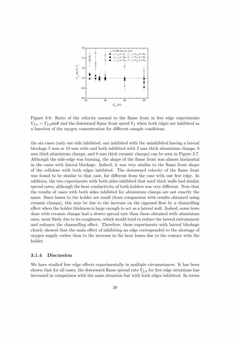
20 30 40 500.6

0.8

1.0

1.2

1.4

1.6

s = 2 s0, w = 2w0

s = 3 s0, w = 2w0

s = 4 s0, w = 2w0

V f,d si

n / V f

XO2

(%)

s = s0, w = w0

s = s0, w = 2w0

s = s0, w = 3w0

s0 = 0.1866 mm; w0 = 2 cm

Figure 3.8: Ratio of the velocity normal to the flame front in free edge experimentsVf,n = Vf,dsinθ and the downward flame front speed Vf when both edges are inhibited asa function of the oxygen concentration for different sample conditions.

the six cases (only one side inhibited, one inhibited with the uninhibited having a lateralblockage 5 mm or 10 mm wide and both inhibited with 2 mm thick aluminium clamps, 8mm thick aluminium clamps, and 8 mm thick ceramic clamps) can be seen in Figure 3.7.Although the side-edge was burning, the shape of the flame front was almost horizontalin the cases with lateral blockage. Indeed, it was very similar to the flame front shapeof the cellulose with both edges inhibited. The downward velocity of the flame frontwas found to be similar to that case, far different from the case with one free edge. Inaddition, the two experiments with both sides inhibited that used thick walls had similarspread rates, although the heat conductivity of both holders was very different. Note thatthe results of cases with both sides inhibited for aluminium clamps are not exactly thesame. Since losses to the holder are small (from comparison with results obtained usingceramic clamps), this may be due to the increase on the opposed flow by a channellingeffect when the holder thickness is large enough to act as a lateral wall. Indeed, some testsdone with ceramic clamps had a slower spread rate than those obtained with aluminiumones, most likely due to its roughness, which would tend to reduce the lateral entrainmentand enhance the channelling effect. Therefore, these experiments with lateral blockageclearly showed that the main effect of inhibiting an edge corresponded to the shortage ofoxygen supply rather than to the increase in the heat losses due to the contact with theholder.

3.1.4 Discussion

We have studied free edge effects experimentally in multiple circumstances. It has beenshown that for all cases, the downward flame spread rate Vf,d for free edge situations hasincreased in comparison with the same situation but with both edges inhibited. In terms

38

of the speed normal to the flame front Vf,n, we may assume that Vf,n = Vf,dsinθ, whereVf,d and θ are measured data. The ratio Vf,n/Vf , where Vf is the flame front velocity forthe two-side inhibited case, as a function of the atmospheric mixture is shown in Figure3.8, where error bars arise from assuming the errors for Vf,d and θ as one standarddeviation of the statistics applied for obtaining them.

From Figure 3.8, we note that Vf,n/Vf = 1 within a 5% range for the thicknesscorresponding to a single sheet, with a slight trend to decrease as XO2 increases whenusing small widths. In these particular cases, large XO2 values imply large inclinationangles, so Vf,n substantially departs from the vertical direction and propagates towardthe inhibited side. The existence of the aluminium clamp two millimetres wide in theinhibited side may substantially reduce the entrainment of fresh air in a similar way as inthe lateral blockage case explained previously. This may lead to Vf,n values smaller thanthe downward flame front velocity Vf obtained with the burning of a sample inhibitedin both sides. We also note that the condition Vf,n/Vf ≈ 1 is not satisfied for largerthicknesses, since the multiple sheets attached together are likely to separate (especiallyin the free edge case), which compromises the assumption of being a single solid fuel.

In comparison with other studies, and from the cellulose-type fuel simulations ofKumar and Kumar [3], we may deduce a ratio Vf,n/Vf = 1.14. It can be shown, however,that a fraction of this 14% difference of flame front spread rates seems to be due to flametemperature differences between the uninhibited and the fully inhibited cases. Thus, wecan calculate the influence of the flame temperature on the front spread rate by usingde Ris’ [27] formula3, Vf ∼ λg/ (ρscs(τ/2)) (Tf − Tv) / (Tv − T∞), where Tf is the flametemperature, Tv is the temperature of vaporization, and T∞ is the ambient temperature.When using the flame temperature corresponding to the free side edge burning case ofKumar and Kumar [3] in the two side inhibited case, the flame front velocity modifiesaccordingly to the dependence of Vf on Tf shown in the expression above. By using thisnew flame front velocity for the inhibited case, the ratio Vf,n/Vf derived from Kumarand Kumar’s [3] data is very similar to 1, with less than a 7% discrepancy.

Once we accepted the relationship Vf,n/Vf ≈ 1, one of our main purposes becameto estimate the downward flame spread from the known experimental conditions. Fordoing this, we derived an upper bound for the downward flame speed Vf,d by applying asimple control volume analysis near the free edge of the sample. This analysis is similarto that developed in Bhattacharjee et al. [18] for two dimensional flames except for theintroduction of a new term corresponding to the lateral heat flux into the sample fromthe free edge side. Three simple control volumes have been used, two in the gas phaseand one in the solid phase, as shown in Figure 3.9. The solid phase control volume is atTv and corresponds to the vaporizing part. There is one gas phase control volume on topof the solid one and another gas phase control volume on the lateral side, both at Tf . Weassume that the solid in front of the control volume shown in Figure 3.9 is at ambienttemperature T∞. Considering that conduction through the gas phase is the main heat

3The de Ris’ model assumes an infinite fast reaction kinetics, so the model here developed may loseapplicability in fires where the chemical kinetics may be slow, as vitiated fires or fires with high flowvelocity.

39

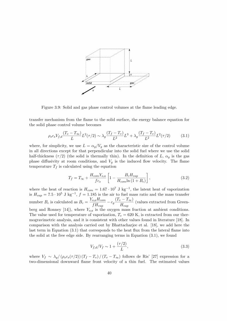
Figure 3.9: Solid and gas phase control volumes at the flame leading edge.

transfer mechanism from the flame to the solid surface, the energy balance equation forthe solid phase control volume becomes

ρscsVf,d(Tv − T∞)

LL2(τ/2) ∼ λg

(Tf − Tv)L2

L3 + λg(Tf − Tv)

L2L2(τ/2) (3.1)

where, for simplicity, we use L = αg/Vg as the characteristic size of the control volumein all directions except for that perpendicular into the solid fuel where we use the solidhalf-thickness (τ/2) (the solid is thermally thin). In the definition of L, αg is the gasphase diffusivity at room conditions, and Vg is the induced flow velocity. The flametemperature Tf is calculated using the equation

Tf = T∞ +HcomYo,afcs

[1− BcHvap

Hcomln (1 +Bc)

], (3.2)

where the heat of reaction is Hcom = 1.67 · 107 J kg−1, the latent heat of vaporizationis Hvap = 7.5 · 105 J kg−1, f = 1.185 is the air to fuel mass ratio and the mass transfer

number Bc is calculated as Bc =Yo,aHcom

fHvap− cg

(Tv − T∞)

Hvap(values extracted from Green-

berg and Ronney [14]), where Yo,a is the oxygen mass fraction at ambient conditions.The value used for temperature of vaporization, Tv = 620 K, is extracted from our ther-mogravimetric analysis, and it is consistent with other values found in literature [18]. Incomparison with the analysis carried out by Bhattacharjee et al. [18], we add here thelast term in Equation (3.1) that corresponds to the heat flux from the lateral flame intothe solid at the free edge side. By rearranging terms in Equation (3.1), we found

Vf,d/Vf ∼ 1 +(τ/2)

L, (3.3)

where Vf ∼ λg/ (ρscs(τ/2)) (Tf − Tv) / (Tv − T∞) follows de Ris’ [27] expression for atwo-dimensional downward flame front velocity of a thin fuel. The estimated values

40

20 30 40 500.0

0.5

1.0

1.5

2.0

2.5

3.0

Eq. (3.3) Data (width = 2, 4 and 6 cm)

V f,d / V f

Figure 3.10: Ratio of the downward flame spread rate Vf,d in the free edge and the flamefront speed Vf when both edges are inhibited as a function of the oxygen concentrationfor samples with 0.0933 mm half-thickness. The solid line corresponds to the estimationprovided by Eq. (3.3).

provided by Equation (3.3) may be seen as upper bounds for the actual Vf,d/Vf figures,since we neglect energy losses in the process.

Figure 3.10 shows the prediction Vf,d/Vf from Equation (3.2) as a function of the oxy-gen mixture concentration in comparison with the values obtained from our experimentsfor the (τ/2) = 0.0933 mm cases. Here Vf,d and Vf correspond to our measured data forboth the free edge and the fully inhibited cases, respectively. Note that L in Equation(3.3) is a function of the oxygen level XO2 through the induced flow velocity Vg. An in-crease in the oxygen concentration will lead to an increase in the flame temperature Tf ,and, therefore, in the buoyant induced flux Vg, which, from Frey and T’Ien [1], satisfies

Vg ∼ [αg (Tf − T∞) /T∞]1/3. Results from Equation (3.3) assume a value of Vg = 0.3 ms−1 for an oxygen mass fraction YO2 = 0.23 [41], with other Vg values in agreement with

Vg ∼ [αg (Tf − T∞) /T∞]1/3, where Tf is the adiabatic flame temperature that dependson XO2 [see Eq. (3.2)].

3.1.5 Conclusions

We have carried out experiments of the downward burning of thin solid fuels with andwithout a free edge and also varying the width and thickness of the sample and the oxygenmolar fraction XO2 in an O2−N2 atmosphere at 105 Pa. The results we obtained showthat the extinction limit that arises when we reduce the width of the sample is attainedat lower values of XO2 for the free edge case in comparison with the fully inhibited one.The flame spread rate of samples with a free edge is greater than in samples without freeedges due to the increase of oxygen supply along the free edge.

The variation of atmospheric composition for the free edge cases not only caused an

41

increase in the velocity of the flame front but also an increase of the inclination of thefront with respect to the horizontal. This implies that the same increase of XO2 has agreater effect in the downward spread rate for free edge samples than in inhibited ones.

Indeed, although the variation of the XO2 affects the angle of the flame front in thefree edge case, our results showed that the velocity normal to the flame front appearedvery similar for samples with one or none free edges for all of our experiments withhalf-thickness (τ/2) = 0.0933 mm. This was not totally satisfied with thicker samples,although we suspect that such a discrepancy may arise from the fact that thicker fuelswere obtained by adding sheets of (τ/2) = 0.0933 mm, which may separate during theburning process, especially in the free edge case.

We did perform studies with samples with both inhibited edges employing holdersof different thermal conductivity. The results showed that lateral heat losses throughthe holders are of minor importance. This was also confirmed when having a lateralblockage close to the free edge, which clarified that the main effect of inhibiting an edgeis the oxygen shortage that it produces, being more important than the increase in theheat losses to the lateral holders. In addition, a simple control volume analysis gave usa reasonable estimate for the downward flame speed along the free edge in terms of theoxygen level concentration.

Acknowledgements

B.C. acknowledges the support of a FPU program grant. J. Vicens and S. Saus pro-vided very helpful technical assistance. P. Bertran and E. Vives obtained some of theexperimental data. This work has been partially funded by the Generalitat de Catalunyaunder grant 2009-SGR-374, the MICINN-FEDER under grant FIS-2009-13050, and theEuropean Commission under grant NEST-28192-FEPRE.

42

3.2 Energy Balance Models of Downward Combustion ofParallel Thin Solid Fuels and Comparison to Experi-ments

This section is a transcription of the contents of the following paper (a copy of thepublished version can be found in Appendix A):

B. Comas and T. Pujol. Energy balance models of downward combustion of parallelthin solid fuels and comparison to experiments. Combustion Science and Technology,185: 1820–1837, 2013.

Abstract

We analyse the flame front speed in the downward combustion of multiple parallel samplesof thermally thin fuels at normal gravity and far from extinction conditions. In contrastwith the single sample case, where conduction through the gas phase is the dominantheat transfer mechanism, in the multiple parallel samples case, radiative heat fluxes maybecome very relevant, which compromises the application of the well-known formula of deRis for determining the burning rate. Here we study the downward combustion of multipleparallel sheets by (1) obtaining new experimental data at different oxygen atmosphericlevels; (2) generalizing a previous comprehensive energy balance model now expectedto be valid for a wide range of scenarios; and (3) deriving an analytical approximationfor the burning rate that generalizes the classical de Ris formula for those cases whereradiative effects cannot be neglected. The comparison with own as well as with externaldata reveals the strengths and weaknesses of these types of models.

3.2.1 Introduction

In a recent work that studied the downward combustion over thin solid fuels, Bhattachar-jee et al. [46] have derived new expressions for describing the main flame geometricalparameters in terms of both gas and solid properties. Here we use these expressionsfor generalizing a comprehensive energy balance model of the downward combustion inmultiple parallel samples. For a single sample, the downward flame front speed in thethermal regime of a thin solid fuel follows the well-known de Ris’s expression [27]:

Vf,deRis =π

4

λg (Tf,ad − Tv)(τ/2) csρs (Tv − T∞)

(3.4)

where the π/4 term has been included after the exact solution derived by Delichatsions[31] (see the Nomenclature for the description of the variables and parameters).

Equation (3.4) assumes that conduction through the gas phase is the main contribu-tion for preheating the virgin solid ahead of the pyrolysis zone. The excellent agreementof the values predicted by Eq. (3.4) with a wide variety of experimental data (see, e.g.,[33]) corroborates that conduction through the solid phase as well as radiative heat fluxesare of secondary importance when burning thin solid fuels far from the extinction limits.

43

This contrasts with the radiative regime found in the microgravity environment wherenatural convection as well as conduction through the gas phase are obviously suppressed.In this case, the flame spread rate strongly depends on radiative effects [18]. At normalgravity and far from the extinction, radiation may also play a major role when multiplesamples are burned simultaneously and radiative heat fluxes emitted from neighbourhigh temperature flames may not be neglected. A strong re-radiation effect also arisesin many real fires caused by the combustion of nearby solids. This has led to studiesof fire propagation at several scales, ranging from bench- to full-scale fire tests. One ofthe intermediate-scale fire tests consists of two parallel samples with a gas burner at thesurface [47, 48]. This parallel panel configuration has been recently employed as a toolfor predicting costly full-scale fire tests (e.g., [49]). In the parallel panel test, samples areburned upward in order to reproduce the most hazardous configuration, and many effortshave been devoted to properly simulate such an upward flame spread (see, e.g., [50]). Insolid fuels ignited at the top, however, flames propagate downward, and the flame frontspeed is substantially lower than that predicted for an upward burning configuration.Therefore, it is important to predict the downward flame spread as accurately as possible.

For an array of cellulosic-type samples, Kurosaki et al. [51] and Itoh and Kurosaki[52] developed a model for the propagation speed of the flame front Vf with a simplifiedexpression for both convective and radiative heat fluxes. Although it correctly predictedthe behaviour of experimental data, Kurosaki and Itoh’s models rely on many valuesextracted from their own data such as flame temperature, height, and length. Thiscompromised the validity of the model when it is used for predicting other scenarios.

The main motivation for conducting the present study was to generalize the compre-hensive model of the downward burning of several parallel samples of Itoh and Kurosaki[52] in order to be fully predictive. This is expected to be accomplished by employing therecent parametrizations of the flame geometry derived by Bhattacharjee et al. [46]. Wealso propose an approximation to our simple model in terms of a simple analytical ex-pression for the flame front speed that generalizes Eq. (3.4) by including radiative fluxesand interaction with multiple samples. The predictions of our models are compared withexperimental data.

3.2.2 Experimental Set-up

Very few experimental works have been devoted to study the downward burning rate ofmultiple parallel cellulosic-type samples. Emmons and Shen [35] analysed the horizontalburning of an array of vertical paper strips. Kim et al. [53] obtained the flame spread ratebetween two parallel fuel surfaces using methanol-soaked slabs as a test fuel. Kurosaki etal. [51] measured the downward flame front speed when two parallel papers were burnedat different separation distances at ambient conditions. This work was generalized byItoh and Kurosaki [52] by burning several papers simultaneously (up to 10) at ambientconditions, whereas micro- and normal gravity studies at low atmospheric pressure ofdownward combustion of two parallel thermally thin solid fuels were carried out by Urbanet al. [54]. Here we obtain new data in the downward burning of parallel thin solid fuelsat different oxygen concentration levels.

44

Figure 3.11: Schematic view of the experimental setup for an array of three papers equallyspaced, with a view of the coiled nichrome wires used to ignite them at the same time.

Our experiments were carried out in a combustion chamber used in our previousresearch [55, 56]. Fuel samples consisted of cellulosic papers of thickness 0.187 mm,width 4 cm, and length 16 cm, which were long enough to ensure a stationary spreadrate but short enough to ensure that oxygen depletion within the chamber was less than2%. Lateral effects due to holders were almost negligible since the flame spread ratewas very similar for samples 4 cm wide and 6 cm wide [56]. Properties of our papersamples are conductivity λs = 0.101 W m−1K−1, density ρs = 461.95 kg m−3, specificheat cs = 1180 J kg−1K−1 (all at 20 oC), and vaporization temperature Tv = 620 K.

Before a test, papers were heated for 2 hours in an oven at 105 oC and 24 h in adesiccator. Sheets of paper were held vertically by aluminium plates 2 mm wide locatedat fixed distances by spacers. Vacuum was made inside the chamber, and then it wasfilled with a mixture of N2 and O2 at the desired proportion with a final pressure of 105

Pa. Gases were mixed with a fan for 2 min. Then, the system rested for 3 min to ensurea correct mixture with no remaining currents inside the chamber as it was confirmed inprevious studies. A coiled nichrome wire placed at the top of each paper ignited themall at the same time. Simultaneity was ensured by using a small amount of nitrocellulosebetween the sample and the wire. In Figure 3.11, we can see an schema of an array ofparallel papers.

Experiments were recorded with a high definition camera as in [52]. The analysisclearly showed the flame front, whose location was obtained from a ruler marked in the

45

Figure 3.12: Image of one experiment. Case N = 2, XO2 = 30%, and C = 28 mm.

edge of the aluminium plate. The spread rate corresponds to the slope of the distance vs.time location of the flame front during a steady propagation. The behaviour of the flamespread rate was the same as that observed or modelled in other studies [51, 52, 54]. Atypical image from the experiments can be seen in Figure 3.12. Note that for experimentswith multiple sheets of paper (i.e., N > 1), the camera was placed in the plane of one ofthe papers in order to assure the alignment of the marks in the holder with the positionof the flame front behind it. We did not take into consideration experiments of parallelsamples that showed delayed flame fronts due to a non-simultaneity of the burning atthe ignition time.

3.2.3 Models

Kurosaki et al. (K) Model

Kurosaki et al. [51] developed a one-dimensional steady flame model (coordinate systemattached to the flame front) for obtaining the downward flame spread rate when burningtwo parallel sheets of paper. Sheets are considered thermally thin, and the physicalproperties of the unburned paper are considered constant. With all these assumptions,the energy balance of an element of the preheated zone of one paper is

λsd2Tsdx2

+ ρscsVfdTsdx

+1

τ(qc + qr) = 0 (3.5)

46

Figure 3.13: Heat fluxes received on an element of the preheated zone of the paper (asin [51], and [52]). See text for details.

where x is the coordinate parallel to the surface, being positive pointing downward (di-rection of propagation) and with the pyrolysis zone starting at x = 0. Note that theequation of propagation exclusively depends on the coordinate of the direction of prop-agation x since the heat fluxes are expressed as a function of x only. The dependenceon the other two coordinates is parametrized in the calculation of the radiative heattransfer rates by using separation distances from paper to flame, from paper to otherpaper C and the width of the samples w (see Figure 3.13). The solution of Eq. (3.5)with the boundary conditions Ts = Tv at x = 0 and Ts = T∞ at x =∞, the assumptionof constant temperature in the pyrolysis zone, and the condition that the temperatureprofile must be continuous and derivable at x = 0 leads to the temperature profile of thepreheated zone,

Ts (x) = Tv −1

ρscsτVf

∫ x

0

[1− eVf (x−ξ)/αs

]q (ξ) dξ (3.6)

where αs = λs (ρscs) is the sample thermal diffusivity. Eq. (3.6) for x =∞ allows us toderive an expression for the flame spread rate,

Vf =Qf

ρscsτ (Tv − T∞)(3.7)

where Qt is the total heat transfer rate per unit width.

Convective qc and radiative qr heat fluxes are calculated for two sheets assuming that

47

emitting surfaces in Figure 3.13 behave as gray bodies, being

qc = λg∂Tg∂y|y=0 (3.8)

qrf1 = aεfσT4f Ff1→dx, qrf2 = aεfσT

4f Ff2→dx (3.9)

qrs = εsσ(T 4s − T 4

∞), qrp

∫ ∞0

aεsσT4s Fdx′→dx (3.10)

qre = aεeσT4e Fe→dx (3.11)

with qrf1 and qrf2 the radiative heat fluxes received from the flame itself and nearbyflames, respectively; qrs and qrp the radiative heat fluxes emitted [negative contributionin Eq. (3.7)] and received from the local and the nearby paper, respectively; and qre theradiative heat flux received from the nearby ember. Thus, for the two parallel sampleproblems, Qt ≡

∫∞0 (2qc + 2qrf1 + 2qrs + qrf2 + qre + qrp) dx (see Figure 3.13).

Kurosaki et al. [51] assume that qc = be−x/δ, with constants b (= 5×104 W m−2) andδ (= 1250 m−1 fitted to reproduce measured data. Radiative heat fluxes use constantflame height Lh (= 0.15 cm), flame length Lf (= 1.5 cm), and ember length Le (= 1.2cm) for calculating the view factors F in Eqs. (3.9), (3.10), and (3.11). The flametemperature Tf (= 1300 K) is set as the mean temperature of the flame region, whereasthe flame emssivity εf = 0.05, the ember emissivity εe = 0.85, and the emissivity εs of thevirgin paper and its absorptivity a with εs = a = 0.92 were taken from previous works.The model also assumes a separation of 0.2 cm along the x direction between the edgeof the flame front and the edge of the ember zone.

Itoh and Kurosaki (I) Model

Itoh and Kurosaki [52] extended the previous model to multiple (N > 2) parallel sheetsof paper by assuming that the total heat transfer rate per unit width for all papers is

QtN = (Qr)i=1 + (Qr)i=N + 2

N−1∑i=2

(Qr)i + 2

N∑i=1

[(Qc)i + (Qrf1)i + (Qrs)i

](3.12)

where Qr = Qrf2 +Qrp +Qre with Qi =∫∞0 qidx for i = c, rf1, rf2, re, rp, and rs.

Since the experiments showed that, after a transient phase, the downward spread ratebecame stationary and equal for all sheets, Itoh and Kurosaki [52] assumed the same heattransfer rate for each sample, this being calculated as

Qt =QtNN

= 2 (Qc +Qrf1 −Qrs) + 2N − 1

N(Qrf2 +Qre +Qrp) (3.13)

which, substituted into Eq. (3.7), allows us to calculate the flame front speed Vf .

In addition, Itoh and Kurosaki [52] expressed both flame Lf and ember Le lengthsas a function of the flame front speed, Le = Vf/K and Lf = ALe, with A (= 0.9) and K(= 0.04 s−1) experimental constants.

48

Generalized Itoh and Kurosaki (I-G) Model

Here we generalize the previous model in order to be totally predictive, thus being onlydependent on the physical properties of the samples and on the ambient conditions.

We assume that the relevant length scale where the convective heat flux qc is impor-tant corresponds to δg ≡ αg/ (Vg + Vf ), as it was determined in [18]. Therefore, we statethat δ = δg in the exponential shape for the convective flux qc = be−x/δ. On the otherhand, we assume that Eq. (3.7) for the one sheet case neglecting radiation must reduceto the de Ris velocity Eq. (3.4) since it is accepted to be valid for the thermal regime.With this condition, the coefficient b of the exponential expression for the convective fluxreads

b =π

4

λgδg

(Tf,ad − Tv) (3.14)

The adiabatic flame temperature used in Eq. (3.14) follows [14],

Tf,ad = T∞ +

(1− 1

1 + YO2/r

)[Tv − T∞ +

1

cg(Hcom −Hvap)

](3.15)

Note also that Tf,ad differs from the flame temperature Tf employed in the calculationof the radiative fluxes, the latter being the mean temperature calculated using the one-dimensional vertical model of a diffusion flame described in [14]. In Eq. (3.15), we usethe mass fraction of oxygen at ambient conditions,YO2; the stoichiometric oxidizer to fuelmass ratio, r; the gas specific heat, cg; the latent heat of vaporization, Hvap; and the heatof combustion, Hcom. The gas specific heat cg in Eq. (3.15) is evaluated at the meantemperature (Tf,ad + T∞) /2 [14].

The opposed flow gas velocity Vg is assumed to vary accordingly to the expression [1]

Vg/Vg,ref = [αg (Tf,ad − T∞)]1/3 / [αg,ref (Tf,ad,ref − T∞)]1/3, where the reference valuescorrespond to those at XO2 = 21% with Vg,ref = 0.3 m s−1.

On the other hand, flame Lf , ember Le, and separation from flame to paper Lhlengths are calculated using Bhattacharjee et al. [46] work:

Lh =1

10rρsρg

τ

YO2

VfVf + Vg

(3.16)

Lf = 0.0345 · 5L2h

Vf + Vgαg

(3.17)

and assuming that the relationship between ember and flame lengths is Le ≈ Lf/0.9 [52].Unless otherwise stated, gas transport coefficient values are evaluated at the vaporizationtemperature [46].

We point out that Bhattacharjee et al. [46] obtain Eqs. (3.16) and (3.17) aftercorrelating data for single sheet cases. We assume here that these expressions are stillvalid for multiple sheets of paper when the separation distance C is reasonably large.Indeed, experimental values for the burning of two parallel sheets of paper revealed thatthe flame structure is essentially the same as for a single sample case when C is above agiven value Cl (e.g., Cl ≈ 10 mm for XO2 = 21% and two parallel samples [51]).

49

Since δ, b, Lh, Lf , and Le depend on the flame spread rate Vf and these terms areneeded in order to compute the total heat transfer rate Qt, an iterative method of solutionhas to be used. On the first iteration, an initial value for lengths is assumed (Lf = 15mm, Le = 12 mm, and Lh = 2 mm), and qrp and qrs are set to 0. The flame spread rateVf and the temperature profile Ts(x) are calculated, and then all the parameters andexpressions are varied accordingly to these new values. This is done iteratively until Vfconverges within a prescribed value (< 0.1% difference).

Analytical (A) Model

The generalization of Itoh and Kurosaki’s model in the previous subsubsection still re-quires an iterative process for obtaining the flame front speed. Here, we derive an an-alytical approximation to the flame spread rate with the aim of generalizing Eq. (3.4)by including radiative effects in the burning of multiple parallel samples. The model isessentially the same as that shown in Figure 3.13 except with the unburned paper regionassumed to have a constant temperature T∞. This substantially simplifies the expres-sions for the radiative fluxes, and a simple energy balance similar to that developed in[18] leads to

Vf = Vf,deRis

[1 +

qrf1qcv

+2 (N − 1)

N

(qrf2 + qre)

qcv

](3.18)

where qcv = πλg (Tf,ad − Tv) / (4δg), qrf1 = aεfσT4f Ff1→1, qrf2 = aεfσT

4f Ff2→1, and

qre = aεeσT4e Fe→1. Here, FS→1 corresponds to the view factor of finite area S (local flame

f1, nearby flame f2 and nearby ember e) to finite area 1 (paper at uniform temperatureT∞; see Appendix). In contrast with the previous subsubsection, values of the parametersδg, Lh, Lf , and Le needed in qcv, qrf1, qrf2, and qre have been evaluated at Vf,deRis insteadof at Vf . This makes Eq. (3.18) fully explicit. Note that in Eq. (3.18) we have neglectedthe contribution of the qrp term due to its small relevance in the total heat transfer rateas noted in [51]. We point out that Eq. (3.18) reduces to Eq. (3.4) for the non radiativecase or for scenarios where conduction through the gas phase qcv is the dominant effect.

3.2.4 Results

One Sample

Figure 3.14 shows the results for a downward burning of one sample at different ambi-ent oxygen molar fractions XO2 . In comparison with data, de Ris expression Eq. (3.4)overestimates the flame speed at low–moderate values of XO2 , whereas it underestimatesit at high XO2 values where radiation, due to high energy flames, may play an impor-tant role. The analytical model (A model in Figure 3.14), which generalizes the de Risexpression by including radiation, predicts higher values of the spread rate due to thepositive contribution of the radiative terms in Eq. (3.18), as already expected. Thisanalytical model matches the data at XO2 = 50% but fails to reproduce the observedbehavior at greater atmospheric concentrations, underestimating by 19% the flame frontspeed at XO2 = 100%. The generalized model gives slightly greater values of Vf than the

50

0 20 40 60 80 1000.0

0.4

0.8

1.2

1.6

2.0

Data (N = 1) I-G model I model K model A model

Vf (

cm/s

)

XO2 (%)

Figure 3.14: Downward burning rate Vf as a function of the oxygen molar fraction XO2

for a single sheet. Our experimental data is compared with the Kurosaki et al. model(K model) [51], Itoh and Kurosaki model (I model) [52], our generalization of Itoh andKurosaki model (I-G model), and an analytical model (A model). Values of Eq. (3.4)are also shown (de Ris).

analytical model, but not higher enough to correctly report the measured data at highXO2 . In comparison with de Ris Eq.(3.4), and for a single sheet, the differences withthe generalized (I-G) model arise from the radiative flux from the flame (qrf1) and theradiative losses from the paper (qrs). This radiative correction may lead to a negativevalue for losses higher than the gain from the flame. However, this is not observed in ourmodel due to the assumed flame shape. In our model, the flame is a rectangle parallelto the paper, separated from it by a length Lh (see Figure 3.13). This provides a viewfactor of the flame to a differential element of the preheated zone of the paper greaterthan it would be if a more realistic shape was assumed, which overestimates qrf1. Notealso that the qrf1 value predicted by the I-G model is greater than the value obtainedfrom the A model since it applies the Vf value instead of the Vf,deRis for determining thegeometrical flame parameters.

In contrast, Kurosaki et al. [51] and Itoh and Kurosaki [52] models clearly under-estimate the experimental observations at moderate–high values of XO2 , only correctlypredicting the flame spread rate at environmental values XO2 = 21%, which correspondto the conditions that they were developed. Both K and I models shown in Figure 3.14adopt a variable value of the flame temperature Tf as a function of XO2 , being the sameas that employed in A and I-G models.

Two Parallel Samples

For two parallel sheets of paper with a separation distance C = 25 mm and burning atdifferent XO2 , Figure 3.15 reveals that I and K models behave better than the generalizedversion at low XO2 . At the maximum XO2 value, the I-G model underestimates Vf by

51

0 20 40 60 80 1000.0

0.5

1.0

1.5

2.0

2.5

Data N = 2, C = 25 mm I-G model I model K model A model

Vf (c

m/s

)

XO2

Figure 3.15: As in Figure 3.14 but for a two parallel sheets case with a separation distanceC = 25 mm.

16%, being similar to the result from the K model, whereas the I model overestimatesit by a 18%. In comparison with the flame front speed obtained for the one samplecase, the generalized model correctly predicts the observed change ∆Vf , thus indicating asuccessful simulation of the effect of the nearby radiative fluxes. This is not accomplishedwhen fixing Lf , Le, and Lh values (K model) or Lf and Le values directly proportionalto Vf (I model), since very high discrepancies in comparison with data are obtained.

Radiative heat fluxes from the local flame qrf1 and the nearby flame qrf2 highlydepend on the flame temperature Tf . As explained above, Tf is obtained by averagingthe vertical temperature profile in a one-dimensional vertical diffusion flame model thatreaches a maximum temperature Tf,ad at the flame height. By applying this procedure,Tf/Tf,ad ranges from Tf/Tf,ad = 0.54 at XO2 = 20% to Tf/Tf,ad = 0.43 at XO2 = 100%.Figure 3.16 shows the results of the flame front speed for two parallel samples separatedC = 25 mm with the generalized I-G model as a function of (a) oxygen molar fraction XO2

and (b) Tf while keeping the Tf,ad value calculated with Eq. (3.15). At moderate–lowlevels of XO2 , the burning spread rate Vf is almost independent of the flame temperature,thus indicating that radiation plays a minor role. However, at larger values of XO2 , weobserve a strong dependence of Vf on Tf since radiative fluxes are becoming important.In comparison with data, a better behavior of the I-G model would be obtained byderiving Tf values from Tf,ad with a different Tf/Tf,ad ratio than that provided by theone-dimensional vertical diffusion model of [14].

In Figure 3.17 we can see the downward spread rate of flames for the two parallelpapers case at XO2 = 30% depending on the separation distance C predicted by the Kmodel, the I model, and our generalization (I-G model). We also include the analyticalA model, and the results obtained with the I-G model when using a characteristic lengthδ = 4δg and a height of the flame Lh 1.5 times that obtained in Eq. (3.16). Thesefigures are chosen in order to produce values of b, δ, Lf , and Lh at XO2 = 21% verysimilar to those adopted in [51]. The latter case correctly reproduces our measured data,

52

20 40 60 80 100

0.2

0.4

0.6

0.8

1.0

1

80

40

20

10T f /

Tf,a

d

XO2 (%)

5

N = 2C = 25 mmI-G model

Figure 3.16: Downward burning rate Vf contours (cm/s) as a function of the ratio betweenthe flame temperature Tf and the adiabatic flame temperature Tf,ad, and of the oxygenmolar fraction XO2 . Nonpropagation is predicted in the gray region. See text for details.

0 10 20 30 40 50 600.0

0.2

0.4

0.6

0.8

1.0

Vf

(cm

/s)

C (mm)

Data I-G model I model K model A model

N = 2, XO2

= 30%

I-G, 1.5 Lh

Figure 3.17: Downward burning rate Vf as a function of the separation distance Cbetween two parallel sheets at XO2 = 30% for the models described in Figure 3.14 andincluding a modified I-G model (see text).

53

0 10 20 30 40 50 600.0

0.3

0.6

0.9

1.2

1.5

1.8

100

60

50

40

30

20

Vf

(cm

/s)

C (mm)

Figure 3.18: As in Figure 3.17 but for the I-G model only and at different oxygen molarfractions (in %).

with a peak at C ≈ 14 mm. Data show a maximum in the spread rate at C = 12 mm(Vf = 0.62 cm s−1), which is 24% higher than the velocity at C =∞ (Vf = 0.50 cm s−1).The behaviour of the flame as a function of the separation distance C is as follows: whenthe separation is narrow, there is no flame between the two sheets and the main heattransfer mechanism is convection. Then there is a transition region, where a unstableflame appears between both papers, and later appears a stable flame between them. Firstit is a united flame and then becomes a separated flame for each paper as the separationbecomes wider. This produces the behaviour observed and predicted for the spread rate:a slow downward flame spread rate when the two papers are separated a small distance,an increase as a function of the separation C with a maximum when the flame betweenthem is higher, and finally the downward spread rate approaches asymptotically that fora single flame. In our observations at XO2 = 30%, and in agreement with the behaviournoted in [51] at XO2 = 21%, the region of a stable flame arises at C > 5 mm, which is wellbelow the region of separation distances that gives a maximum in the flame front speed(10 < C < 15 mm; see Figure 3.17). Note that models tested here are only applicable forC values large enough to ensure that a stable flame exists between papers (i.e., C > 5mm). In those very few cases where the simulation predicts a flame height Lh higherthan half the separation distance C between papers, we force Lh to be C/2.

In Figure 3.17, the analytical A model does not show an abrupt peak at intermediatevalues of the separation distance. This may be caused by the simplified expression of theradiation effects that employs a view factor between two finite areas. The generalizedI-G model reproduces the behaviour of data, with a maximum velocity at C = 11 mmbut at a higher value (0.84 cm s−1).

The effect of increasing the oxygen concentration level is shown in Figure 3.18 for theI-G model. The maximum in the flame front speed shifts to lower values of the separationdistance C as the oxygen molar fraction XO2 increases. However, at large XO2 values,the region with a stable flame between papers will begin at larger C values than at low

54

0 10 20 30 40 50 600.0

0.1

0.2

0.3

I-G, 1.5 Lh, 4 g

Data (Kurosaki et al., 1979) I-G model I model K model A model

Vf

(cm

/s)

C (mm)

N = 2, XO2

Figure 3.19: As in Figure 3.17 but for cellulosic-type samples as in Kurosaki et al. [51].See text for details.

XO2 . Thus, at high XO2 conditions, this implies that the maximum in the flame speedwill arise just at the point C of formation of a stable flame between papers.

Finally for the two parallel sheet problem, we have also analysed the data obtainedin [51]. Samples have the following properties ks = 0.577 W m−1K−1, ρ=901 kg m−3,cs = 1670 J kg−1K−1, and τ = 0.2 mm with Tv = 533 K and Te = 800 K. The experimentwas carried out at XO2 = 21% and T∞ = 298 K. Results are shown in Figure 3.19 wherethe generalized I-G model with the modified Lh and δ parameters also performs betterthan the other models, including the Kurosaki et al. [51] one (K model), that was fittedto reproduce the data.

Multiple (N > 2) Samples

We have also simulated the effect of using a high number of samples, and the results ofthe flame speed as a function of the separation distance C are shown in Figure 3.20 forthe XO2 = 30% case. Experimental data shown in Figure 3.20 have been obtained in ourcombustion chamber with C = 15 mm. For comparison purposes, the I model has beenalso shown. Note that the solution reaches an asymptotic value as N increases, with themaximum in the burning rate shifted to higher C. As expected, the contribution of morepapers increases the total heat available, and therefore the flame front speed Vf alsoincreases. Note that the I model assumes a very strong dependence of Vf as a function ofN due to the overestimation of the radiation fluxes previously explained when discussingFigure 3.15.

3.2.5 Conclusions

We have compared several comprehensive energy balance models developed for derivingthe downward flame front speed Vf in the burning of parallel thin cellulosic-type samples.In these cases, a model beyond the classical de Ris [27] one is needed since radiation may

55

0 10 20 30 40 50 600.1

0.5

0.9

1.3

2

4

1

2

5

10

5

2

Vf

(cm

/s)

C (mm)

Data I-G model I model

XO2 = 30%

11

Figure 3.20: Downward burning rate Vf as a function of the separation distance Cbetween two parallel sheets at XO2 = 30% for different number of parallel samples. Itohand Kurosaki model (I model) and our generalized model (I-G model) are shown.

play an important role. The Kurosaki et al. [51] model (K model) uses constant values ofthe main flame geometrical dimensions and flame temperatures. The Itoh and Kurosaki[52] model (I model) assumes flame and ember lengths proportional to Vf . Our general-ization of the I model employs the parameterizations of the flame geometrical dimensionsof Bhattacharjee et al.[46] and a variable convective flux (I-G model). In addition we de-rive an analytical expression (A model) that employs a simplified expression for radiativeheat fluxes with a constant temperature for the unburned solid.

K and I models show a good performance at ambient conditions (XO2 = 21%) only,since they have several parameters estimated using experimental data. At other XO2

atmospheric levels, these models clearly fail to predict the burning rate of a single and/orof two parallel sample cases. In comparison, our generalized I-G model better predictsthe observed behavior for a wider range of XO2 concentration (up to 50%). For very highvalues of XO2 , however, the I-G model underestimates Vf since the approximation of theflame as a sheet parallel to the surface of the paper may not be appropriate enough, andmay produce radiative heat fluxes values lower than the actual ones.

For a fixed (moderate to low) XO2 concentration, the behaviour of the burning rateas a function of the separation distance between parallel papers is very well predicted byour (slightly modified) I-G model when comparing with our experimental data as well aswith data obtained by [51] with a different type of solid fuel.

These comprehensive models contrast with the recently developed model of Shih [57]that explicitly includes fluid dynamics and is able to simulate both counter and coflowconditions. However, such a type of model requires costly methods, which limits thenumber of cases that can be studied.

As we have shown here, energy balance models may capture the essential physics ofthe problem and correctly reproduce flame front speed data in a wide variety of cases.Therefore, we think that there is still room for this type of modelling as long as they

56

Figure 3.21: View factor of surface S1 to a differential strip dx (K, I, and I-G models).

keep their simplicity. Indeed, a simpler model than the one shown here has been usedby Bhattacharjee et al. [18] with the purpose of deriving a flammability map in themicrogravity regime. For multiple parallel sheets, our results suggest the need of a goodcalculation of radiative fluxes for better determining the downward flame spread in awider range of atmospheric oxygen concentration.

Acknowledgements

B.C. acknowledges the support of a FPU grant. Jordi Vicens and Sergi Saus providedvery helpful technical assistance. J. Jaggopota obtained some of the experimental data.This work has been partially funded by the Generalitat de Catalunya under grant 2009-SGR-374 and the MICINN-FEDER under grant FIS-2012-31307.

Appendix: view factors

Surface S1 to a differential strip dx (Figure 3.21):

Fs1→dx =1

π

[√B2 + C2

B

(tan−1

A+ x√B2 + C2

− tan−1x√

B2 + C2

)− C

B

(tan−1

A+ x

C− tan−1

x

C

)

+A+ x√

(A+ x)2 + C2

tan−1B√

(A+ x)2 + C2

− x√x2 + C2

tan−1B√

x2 + C2

(3.19)

Surface S1 to surface S2 (Figure 3.22):

Fs1→s2 =1

S1

2∑l=1

2∑k=1

2∑j=1

2∑i=1

(−1)i+j+k+lG (xi, yj , ηk, ξl) (3.20)

57

Figure 3.22: View factor of surface S1 to a surface S2 (A model).

G =1

2π(y − η)

[(x− ξ)2 + z2

]1/2tan−1

y − η[(x− ξ)2 + z2

]1/2

+1

2π(x− ξ)

[(y − η)2 + z2

]1/2tan−1

x− ξ[(y − η)2 + z2

]1/2

− z2

4πln[(x− ξ)2 + (y − η)2 + z2

](3.21)

58

3.3 Flame front speed and onset of instability in the burn-ing of inclined thin solid fuel samples

This section is a transcription of the contents of the following paper (a copy of thepublished version can be found in Appendix A).

B. Comas and T. Pujol. Flame front speed and onset of instability in the burning ofinclined thin solid fuel samples. Physical Review E, 88: 063019, 2013.

Abstract

We focus on the front propagation of diffusive flames obtained from the downward burningof inclined thermally thin solid fuels. This process consists of a pyrolysis reaction in thesolid phase and a combustion reaction in the gas phase. The solid phase model is basedon two coupled one-dimensional equations of temperature and solid density. We reducethe system into a single one-dimensional equation from which we obtain an analyticalexpression for the flame front speed. This expression may be understood as an upperbound of the burning spread rate in inclined samples. The gas phase model is basedon four coupled two-dimensional equations. These are employed to derive a criterionfor determining the critical inclination angle beyond which the flame behaviour becomesunstable. The comparison with the experiments confirms the validity of our predictions.PACS numbers: 47.70.Pq, 47.70.Fw, 47.20.−k, 82.33.Vx

3.3.1 Introduction

Combustion is an exothermic process of chemically reacting flows that may produceeither a premixed or a nonpremixed flame [58]. Premixed flames occur when both fueland oxidizer are mixed before burning. In laminar flows of flat premixed gaseous flames,several methods applied to the one-dimensional reaction-convection-diffusion equationsthat correspond to the conservation equations of mass and energy lead to analyticalapproximations of the flame front speed [59, 60, 61].

On the other hand, diffusion (or, equivalently, nonpremixed) laminar flames arisewhen the mixing and burning occur simultaneously, like in the downward burning of acellulosic type sample. In contrast with flat premixed gaseous flames, the combustion ofthin solid fuels is, at least, a two-dimensional process, since it involves the mass flux ofvolatiles at the solid surface and the combustion reaction at the flame height. For such aprocess, analytical expressions for the speed of the flame front Vf have been obtained afterreducing complex two-dimensional reaction-convection-diffusion equations into a singleone-dimensional one [5, 56]. Although some of these approximations successfully predictthe downward flame speed, they fail to explain the burning spread rate over inclinedsamples where flame instabilities may arise [62].

In this work, we use the solid phase equations in Subsec. 3.3.3 to derive an analyticalexpression of the upper bound of the flame spread rate. This expression generalizesprevious equations and it is valid for inclined surfaces. In Subsec. 3.3.4 we use thegas phase equations to obtain stationary solutions that allow us to calculate the Nusselt

59

Figure 3.23: Schema of the combustion chamber.

number at first-order approximation (equivalent to assume only the gravity componentparallel to the surface) and at second-order approximation (equivalent to assume thegravity component normal to the surface). A given value of the ratio of these Nusseltnumbers will provide an instability threshold when comparing with experimental data asshown in Subsec. 3.3.5. Here, our approach differs from Refs. [21, 63] since it is basedon the fundamental governing equations.

3.3.2 Experimental setup

The experiments were carried out in a combustion chamber, using a controlled atmo-sphere of 105 Pa with a mixture of O2 and N2. Figure 3.23 shows a schematic view of theexperimental design. The combustion chamber could be inclined at the angle requiredfor the test.

Cellulosic samples of half-thickness 0.0933 mm and surface density 0.0431 kg m−1

were used. The length and width of the samples were 24 × 4 cm, long enough to ensuresteady spread and wide enough to minimize effects of lateral heat losses. More detailsabout the samples and justification of the sizes can be found in Ref. [8].

Samples were dried for 2 h at 100 oC and stored for a minimum of 24 h before eachexperiment. Then they were held by aluminium holders, 2 mm thick and 40 mm wide,in the middle of the chamber; the chamber was closed and inclined to the desired angle.A vacuum was created inside the chamber and then it was filled with O2 and N2 at thedesired concentration. Gases were mixed during three minutes with a fan and then theywere left at rest for 2 min. Samples were ignited uniformly at the top with a coilednichrome wire. Three repetitions with the same sample configuration and atmospheric

60

Figure 3.24: Image from one experiment made at 30% of O2, with an inclination of 70o

respect to the horizontal.

concentration were done.

Every experiment was recorded with a high-definition camera at 50 Hz. Videos werelater analysed frame by frame to determine the position of the flame front and theexistence (if observed) of an erratic flame behaviour that may cause instabilities andproduce a substantial variability of the flame front speed once the experiment is repeatedunder the same conditions. A typical image of the experiment can be seen in Fig. 3.24.Flame spread velocities were obtained through lineal regression of the front position withrespect to time, with a correlation factor of 0.996 or better for all cases.

3.3.3 Flame spread rate

The combustion of a vertical cellulosic-type sample ignited at the top produces a flamefront that propagates downwards at a given speed Vf . For thermally thin solids, manyauthors have proposed analytical expressions for calculating Vf based either on an energybalance of the solid phase [46] or on an energy balance of the gas phase [56]. Here, wegeneralize the broadly accepted model of de Ris [27] based on the solid phase equationsin order to study the flame spread rate of inclined samples. This model assumes unitLewis number (equal thermal and mass diffusivities) and constant transport coefficients.

The burning process of cellulose consists of two main chemical reactions. The firstis the endothermic pyrolysis reaction in the solid phase that releases fuel volatiles. Thesecond is the exothermic combustion reaction in the gas phase (oxygen and fuel volatiles)that produces a diffusive flame. The transfer of heat from the flame to the virgin solidahead preheats the sample, produces the pyrolysis, and sustains the propagation of theflame front.

The governing equations for the solid phase temperature Ts and solid phase density

61

ρs are

csρsdTsdt

= −∇ ·−→Js − dρs

dt [Hvap + (cs − cg) (Ts − T∞)] (3.22)

dρsdt

= −Asρse−Es/(RTs) (3.23)

where cs and λs, used in the conductive heat flux term, are the specific heat and conduc-tivity of the solid, Hvap is the heat of vaporization, cg is the gas specific heat, and T∞ is

the room temperature. The term−→Js in Eq. (3.22) includes radiative as well as conductive

heat fluxes. In Eq. (3.23), Es and As are the activation energy and the preexponentialterm of the pyrolysis reaction, respectively, with R the universal gas constant.

By applying the classical analysis of Benguria and collaborators [59] to the set of Eqs.(3.22) and (3.23), Ref. [8] obtained an upper bound of the flame front speed,

Vf < Vf,deRis − 2

∫ 1

02√Fθsdθs (3.24)

where

F =αsTvAsρse

−Es/(RTs) [Hvap + (cs − cg) (Tv − T∞) θs] d

c2sρ2s∞ (Tv − T∞)2

(3.25)

with αs the solid thermal diffusivity, T∞ and Tv the room and the vaporization temper-atures, respectively, θs a dimensionless variable defined as

θs =(Ts − T∞)

(Tv − T∞)(3.26)

and d a function of θs such as d = 0 at θs = 1 and d = 1 at θs = 0.In Eq. (3.24), the term

Vf,deRis =2λg (Tf,ad − Tv)τcsρs∞ (Tv − T∞)

(3.27)

corresponds to the de Ris equation with τ the solid thickness, λg the gas phase conduc-tivity and Tf,ad the adiabatic flame temperature (excluding a π/4 multiplying factor thatarises after solving the gas phase equations).

Equation (3.24) applies only to the downward combustion of vertical samples. In thisconfiguration, the background convective flow induced by density variations through theflame region opposes the direction of propagation of the flame front. However, as theangle of inclination of the sample increases, the convective flow parallel to the sampledecreases in intensity and, therefore, the velocity of the flame front increases. Here, wedevelop an analytical expression that aims to include this effect.

According to Ref. [64], our model assumes no pyrolysis (constant solid density) aheadof the flame front. Then, in a coordinate system attached to the flame front, Eq. (3.22)applied to the preheated region (negative x′) reduces to

csρsVfdTsdx′

= λsd2Tsdx′2

− ∂Js∂y

. (3.28)

62

The integration of Eq. (3.28) through the sample thickness (from y = −τ to y =0) and with the dimensionless variables θs (3.26) and x = x′/Lgx+ with Lgx+ as thecharacteristic gas phase thermal length along x (parallel to the solid surface) of theupper side + of the inclined sample leads to

Vfdθsdx

=αsLgx+

d2θsdx2−

− Lgx+τcsρs (Tv − Ts∞)

(Jcv,y=0 − Jcv,y=−τ + Jrd,y=0 − Jrd,y=−τ ) ,

(3.29)

where Jcv and Jrd are the conductive and radiative heat fluxes on the upper y = 0 andlower y = −τ sides of the inclined sample. In Eq. (3.29), we have assumed a uniformtemperature across the y direction within the paper sample, which agrees with the thinsolid fuel case studied.

The conductive flux in the preheated region is commonly expressed in terms of ex-ponentially decaying functions with a maximum value at the flame leading edge (x = 0)[52, 64]. At this point, we assume the adiabatic flame temperature Tf,ad as the charac-teristic gas phase temperature and Tv as the characteristic solid temperature. Therefore,the conductive heat flux at the solid surface at x = 0 is equal to λg (Tf,ad − Tv) /Lgywith Lgy the characteristic thermal length along y. Thus, the upper Jcv,y=0 and lowerJcv,y=−τ conductive fluxes in the preheated region are

Jcv,y=0 = −λg (Tf,ad − Tv)

Lgy+ex, Jcv,y=−τ =

λg (Tf,ad − Tv)Lgy−

exLgx+/Lgx− , (3.30)

where Lgy+, Lgy− and Lgx− are the characteristic gas phase thermal lengths along y orx in the upper + or lower − sides of the inclined sample.

The radiative flux emitted by the flame and absorbed at the virgin solid ahead of theflame front is obtained by using a simplified model in which both flame and paper areconstant temperature planes that intersect at the flame leading edge. From the above,the integration of the radiative fluxes from x = −L/Lgx+ to x = 0, where L is the lengthof the paper, gives∫ 0

−L/Lgx+

(Jrd,y=0 − Jrd,y=−τ ) dx = εfaσT4f

(F+s−f + F−s−f

) L

Lgx+(3.31)

where εf is the flame emissivity, a is the absorptivity of the paper and Tf is the meanflame temperature. As pointed out in Ref. [52], Tf must be lower than the adiabaticvalue Tf,ad and here is taken as the mean value of the gas phase temperature obtainedin the one-dimensional flame model of Ref. [14]. The view factors from the paper planeto the flame plane are

F+,−s−f =

1

2

1 +LfL−

√1 +

L2f

L2− 2

LfL2

cosβ+,−

(3.32)

63

with β+ and β− the angle between the flame plane and the paper plane in the upper andlower sides of the sample, respectively.

The integration of Eq. (3.29) from x = −L/Lgx+ to x = 0 gives

Vf,g =αsLgx+

dθsdx

∣∣∣∣x=0

+2αsτ

λg (Tf,ad − Tv)λs (Tv − Ts∞)

[Lgx+Lgy+

(1− e−L/Lgx+

)+Lgx−Lgy−

(1− e−L/Lgx−

)] αsτ

εfaσT4fL

λs (Tv − Ts∞)

(F+s−f + F−s−f

).

(3.33)

Note that Eq. (3.33) for the case with no radiation and no conduction through thesolid phase reduces to the classical de Ris Eq. (3.27) for Lgx+ = Lgx− = Lgy+ = Lgy−and L = ∞ as it should. Also note that for our radiative calculation, the temperatureof the virgin solid is assumed constant and equal to that for the room. This implies nonet radiative losses that would tend to lower the velocity in Eq. (3.33). Therefore, Eq.(3.33) will overestimate the flame front speed and may be understood as an upper boundto the actual value. This is confirmed by comparison with the experiments as we showin Subsec. 3.3.5.

3.3.4 Instability

The momentum and continuity gas phase equations for a steady diffusion laminar flameupon an inclined angle φ from the vertical are the starting point of the instability analy-sis. The classical analysis of these equations ignores the gravity component normal to thesurface [53, 65, 66], either by considering only vertical combustion or low-enough incli-nation angles φ. Our analysis aims to find the critical point where instability arises, andsince it is located at angles near π/2, we must maintain the gravity component normalto the surface. This implies a nontrivial equation for the normal momentum that cannotbe solved analytically.

In this subsection the flame plane is modelled parallel to the surface of the paper(β+ = β− = 180o in Eq. (3.32)) in order to use Boussinesq approximation for thedensity. We note that the flame speed Eq. (3.33) decreases by less than 4% only whenvarying the β angles from 140o to 180o for the 30% oxygen concentration case. We haveexperimentally seen with the aid of lateral mirrors inside the combustion chamber thatthe flame plane does not substantially deviate from the surface until the angle is close tothe horizontal, where the flame becomes unstable.

Continuity, momentum, and energy equations will be

∂ (ρu)

∂x+∂ (ρv)

∂y= 0 (3.34)

u∂u

∂x+ v

∂u

∂y= ν

∂2u

∂y2+ gcosφ

(ρ∞ − ρ)

ρ(3.35)

u∂v

∂x+ v

∂v

∂y= ν

∂2v

∂y2+ gsinφ

(ρ∞ − ρ)

ρ(3.36)

u∂ (T − T∞)

∂x+ v

∂ (T − T∞)

∂y= α∇2 (T − T∞) (3.37)

64

where boundary-layer assumptions have been made [53, 65, 67]. In the above equationswe have supposed constant transport properties, unit Lewis number, and velocities muchless than the speed of sound. Equations (3.34), (3.35), (3.36), and (3.37) provide thestarting point of a natural convection flux. From these equations we can reach theequations in integral form,

ν∂2u

∂y2

]δ0

+ gcosφρ∞ − ρρ

]δ0

− gsinφ∫ δ

0

∂

∂x

(ρ∞ − ρρ

)dy = 0 (3.38)

∂

∂x

∫ δ

0u(T − T∞)dy − α ∂(T − T∞)

∂y

]δ0

= 0 (3.39)

The detailed analysis from Eqs. (3.34), (3.35), and (3.36) to the equations in integralform is not given here for the sake of brevity and may be found in the literature [53, 68].For a downward (or inclined) spreading flame, the reference frame is defined as travelingat the steady flame spread rate Vf . The boundary conditions of the fluid will be

u = Vfρ = ρfT = Tf

for y = 0 (3.40)

u = VfT = T∞ρ = ρ∞∂u∂y ,

∂(T−T∞)∂y , ∂[(ρ∞−ρ)/ρ]∂y = 0

for y = δ (3.41)

The assumed velocity profile is similar to the velocity profile obtained in the numericalmodel of Ref. [11],

u = u1y

δ

(1− y

δ

)2+ Vf (3.42)

where δ is the thickness of the boundary layer. The density profile is normalized from 1to 0,

(ρ∞ − ρ)ρf(ρ∞ − ρf )ρ

=(

1− y

δ

)2. (3.43)

Setting these profiles in the integral equations (3.38) and (3.39) gives a set of differentialequations that in dimensionless form are

6u′1δ′2

= PrGrcosφ+1

3sinφPrGr

dδ′

dx′(3.44)

1

30

d

dx′(u′1δ′Gr)

= 2Gr

δ′(3.45)

where the dimensionless quantities are u′1 = u1L/α, δ′ = δ/L, x′ = x/L, being L acharacteristic length scale. The Grashof and Prandtl numbers are defined as follows:

Gr = gρ∞ − ρfρref

L3f

ν2ref(3.46)

Pr =νrefαref

(3.47)

65

where the subscript ref means that properties are evaluated at the reference temperature.The set of dimensionless equations (3.44) and (3.45) might be solved for an inclined platefirst neglecting the term with dδ′/dx from both equations. This is equivalent to consideronly the gravity component parallel to the surface. This first approximation gives

δ′1 =(

480PrGrcosφ

)1/4x′1/4 (3.48)

u′1,1 =(403

)1/2(PrGrcosφ)1/2 x′1/2 (3.49)

The Nusselt number is the ratio of the heat transfer convected by the heat transferconducted. For natural convection, it is a function of Prandtl and Grashof numbers [67].It may be expressed as Nu = 2/δ′ [53]. Then

Nu1 =2

4801/4(PrGrcosφ)1/4 (3.50)

Taking into account the gravity component normal to the surface allows us to makea second approximation,

δ′2 = δ′1

[1− 1

6 tanφ(

480PrGrx′

)1/4]1/21− 1

3 tanφ(

480PrGrx′

)1/4 (3.51)

u′1,2 = u′1,1 +103/4

35/4tanφ

(PrGrcosφ

x′

)1/4 1− 16 tanφ

(480

PrGrx′

)1/4[1− 1

3 tanφ(

480PrGrx′

)1/4]2 (3.52)

where the second approximation to the Nusselt number gives

Nu2 = Nu11− 1

3 tanφ(

480PrGr

)1/4[1− 1

6 tanφ(

480PrGr

)1/4]1/2 (3.53)

3.3.5 Results

Figure 3.25 shows the experimental results of the flame spread rate as a function of theangle of inclination of the sample for (a) different values of room oxygen concentration(new data, three repetitions on every environmental conditions) and (b) ambient condi-tions obtained by Refs. [26] and [69]. In Ref. [62] there was also an experimental analysisof the flame front speed for different angles of inclinations but with an external heatingsupply. In contrast with the results of Kurosaki and coworkers [26, 69], Kashiwagi andNewman [62] found that there exists a threshold angle of inclination beyond which theinstabilities of the flow lead to large variations on the value of the flame front speed. Thiscritical angle reduces as the value of the external heat supplied to the system increases.This effect is not clearly observed at near-ambient conditions without an external heatsupply. However, at higher room oxygen concentration XO2 , we do capture an onsetof instability (see Fig. 3.25) that arises at lower angles of inclination as XO2 increases.

66

Figure 3.25: Flame spread rate versus angle to vertical of the samples.

0.0

0.5

1.0

1.5

2.0

2.5 Ref. [26] Ref. [69]

Vf/V

f,deR

is XO2

= 22% X

O2 = 30%

XO2

= 50%

101 102 103 104 1050.0

0.5

1.0

1.5

2.0

2.5 Ref. [26] Ref. [69]

Vf/V

f,g

Da

XO2

= 22% X

O2 = 30%

XO2

Figure 3.26: Normalized values of flame front speed as a function of Damkohler number.5

Note in Fig. 3.25 that the flame spread rate is almost constant for a wide range of an-gles of inclination until a point where the three repetitions of the experiments produce avariation of 20% or higher between flame spread values.

Although such an instability makes it difficult to reproduce the observed flame spreadrate by means of an analytical model, a generalization of the de Ris expression (3.27)in order to predict the trend of data is of great importance, especially at low oxygenconcentrations. Figure 3.26 shows the normalized values of the flame front speeds shownin Fig. 3.25 as a function of the Damkohler number Da. In Fig. 3.26, Vf,deRis follows Eq.(3.27) and Vf,g is obtained from Eq. (3.33) by using the characteristic gas phase thermallengths as

Lgx+ =αg

Vacv cosφ+ Vf, (3.54)

5The x-values of this figure are different from those of the article as we found an error in the Damkohlernumber calculations. It has no implications in the conclusions of our work.

67

and Lgx− = Lgy+ = Lgy− = Lgx+(φ = 0o). In Eq. (3.54) αg is the gas phase thermaldiffusivity and Vacv is the convective velocity itself, which is calculated as Vacv = [gα(ρ∞−ρf )/ρref ]1/3 (the formula is obtained equating buoyancy and inertia forces [11]). Notethat Vacv cosφ is the component parallel to the sample surface on the upper side. Below,the paper acts as a barrier for the upward convective flow and, for simplicity, we haveemployed Lgx− = Lgy+ = Lgy− = Lgx+(φ = 0o). The effect of the radiative flux fromthe flame is taken into account by using a constant value of β+=β− = 140o, althoughdifferent values of these angles did not produce significant changes on the burning rate,which confirms the small relevance of radiative fluxes in the flame front propagationwithin the thermal regime [18]. Conduction through the solid in Eq. (3.33) has been alsoneglected, since it is not considered of importance in the burning of thin samples [5].

The Damkohler number is the ratio of the residence time for the gas mixture in theflow and the chemical time for the second-order Arrhenius-type reaction [33], being

Da =αgρg

YFYOAge−Eg/RTf,ad

(Vacv cosφ+ Vf )2(3.55)

where Ag(= 3.57×107 m3 kg−1 s−1) is the preexponential factor, Eg (= 125×105 J mol−1)is the activation energy and YO and YF are the room oxygen and fuel mass fractions,respectively. Following [33], the fuel mass fraction follows YF = Sc ln(1+Bc)/B

0.15c where

Bc is the mass transfer number and Sc is the viscous to mass diffusivity ratio. We notethat higher values of the Damkohler number are obtained for higher values of inclinationangle and/or higher values of room oxygen concentration level (fast reaction).

In Fig. 3.26, the normalized flame front speed data with respect to the de Ris ex-pression shows a trend to increase as a function of the Damkohler number Da. A similarbehavior was already observed in Ref. [33] for the downward (φ = 0o) combustion ofthin solid fuels. Our simple analytical model (3.33) improves the classical one since thenormalization of Vf with Eq. (3.33) tend to be almost independent on Da. However, Eq.(3.33) overpredicts the flame front speed for a factor of 1.3 to 5, depending on the dataand angle employed. In contrast with the classical de Ris expression, however, Eq. (3.33)behaves as an upper bound whose range of values are even below than those obtainedapplying Eq. (3.24) (see Fig. 3 in Ref. [8]).

The onset of the instability can be tracked using the quotient of Nusselt numbersexposed in Subsec. 3.3.4. Figure 3.27 shows the ratio of Nusselt numbers calculated asin Eq. (3.54) for all the situations tested and the theoretical behavior expected. There isa good agreement between the expected curves and experimental values of the quotientof Nusselt numbers; they differ less than 1.5%. The values of Nu2/Nu1 = 0.9 are chosenas the theoretical critical angle in Fig. 3.27, being 64.2 and 55.4 for XO2 = 30% and50%, respectively. This coincides with the experimental angles showing unstable valuesseen in Fig. 3.25. For the XO2 = 22% case, there is no instability due to the low energyof the flame as also observed in thermally thicker samples [26, 69].

The Grashof number is computed using as a reference length the flame length Lf , cal-culated using the formula obtained in [46], Lf ≈ 0.0345 {(Tf− Tv)/ [(Tv − T∞)YO2∞]}2 α/(Vacv+Vf ), with the flame spread rate Vf being either the experimental value or the calculated

68

0 20 40 60 800.70

0.75

0.80

0.85

0.90

0.95

1.00

critical anglefor X

O2 = 30%

critical anglefor X

O2 = 50%

Nu 2/Nu 1

Angle (deg)

XO2

= 22% X

O2 = 30%

Figure 3.27: Nu2/Nu1 for all XO2 tested, experimental results and expected curves.

using de Ris’ formula (Vf = (π/4)λ/(τρscs)(Tf − Tv)/(Tv − T∞) [27], i.e., Eq. (3.33) forφ = 0o with no radiation neither conduction through the solid phase). The experimentalvalues of the flame length were not used because of experimental difficulties. The tem-perature of flame used is the mean of temperatures of the flame zone computed as in[14]. The reference temperature used for calculating the transport properties from thegas was the vaporization temperature (Tv = 620 K).

For nearly horizontal samples, the experiments show an unstable spread rate thatmay be triggered by curling of ashes and may be due to the flame in the lower side ofthe sample, as stated in Ref. [62]. The instability observed can be explained through theimportance of the gravity component normal to the surface.

The importance of the normal component of gravity can be traced through the cor-rection done to the Nusselt number Nu2/Nu1. After doing the tests, it has been seen thatwhen this correction is greater than 10% of Nu1, flame spread rates become unstable andexpand for a large range of values.

3.3.6 Conclusions

The flame spread down thermally thin inclined samples is controlled by heat transfer tothe unburned part of the sample. For vertical or slightly inclined surfaces, the behaviorcan be explained using only the component of gravity parallel to the surface. The com-ponent of gravity normal to the surface of the sample gains importance as the surfacebecomes more horizontal and may trigger an instability. In this paper we have general-ized the classical analytical expression of the flame front speed [27] in order to be validfor the downward burning of an inclined sample. We have also developed a method toshow the importance of the normal component of gravity via the quotient of Nusseltnumbers having and not having into account this component. We have found that theinstability arises when the correction is greater than a 10%, this being valid for differentXO2 concentration values.

69

Acknowledgements

B.C. acknowledges the support of a FPU grant from the MICINN. Some data were ob-tained by Adria Carmona. We also thank Jordi Vicens and Sergi Saus for their technicalassistance. This work has been partially funded by the Generalitat de Catalunya underGrant No. 2009-SGR-374 and the MICINN-FEDER under Grant No. FIS-2012-31307.

70

Chapter 4

Discussion

Since the results of this Ph.D. thesis has been published in three articles, the previoussections of the results chapter contain separated discussions. The present chapter aimsto unite them in order to have a deeper insight of the flame spread problem.

4.1 Comparison with previous studies

Previous authors have dealt with the flame spread problems here analysed. In thissection, we list the studies that, at our knowledge, have experimentally worked on thetopics discussed in Section 3.1, 3.2 and 3.3. Thus, the following tables contribute to putour results in the context of the current knowledge of the flame front propagation overthin solid fuels.

Table 4.1 summarizes the main features of the works carried out by other authors inthe study of the side effects on the burning of thin sheets. In addition, we also include datacorresponding to the work done in Section 3.1. We point out that Table 4.1 reproducesTable 3.1 found in Section 3.1. Note that our study extends the previous works byanalysing the effects of using lateral walls. These tend to reduce the lateral entrainmentof air. This blockage phenomenon has been here investigated for the first time by usinglateral holders of different materials. This has shed light into the relevance of the heatconduction through the holding plates as discussed in the following subsection.

The case of burning multiple parallel thin sheets has been investigated by a morereduced number of authors. The list of the previous works on this topic, including theircharacteristics, is found in Table 4.2. The first studies carried out by Ref. [70] werefocused on explaining the channel effect of two burning surfaces. They found the spreadrate and the temperature profile without radiation and assuming an infinite combustionreaction rate of plates soaked in methanol, heptane and cellulose. They concluded thatthe flame front speed was controlled by the Grashof number and the length and width ofthe channel. A great step on the understanding of this problem was due to the excellentpaper of Kurosaki et al. [51] who not only derived a comprehensive, physically-based

1Exp.= Experimental, Sim.= Simulation, in.= Inhibited, A= Air2Assuming ρs = 1160kgm−3

71

Ref. Method Case Fuel w ρs(τ/2) XO2 Results1

(cm) (kg m−2) (%)

[3] Sim. 1 in. edge,2 in.edges

Cellulose 2 0.046 20 to25

Vf,d,θ, fluidfields,etc.

[23] Exp. 1 in. edge Fabric,PMM

14 0.2057(andothers)

A Vf,d

[36] Exp. 1 in. edge PMMA 8 0.58 to3.482

A Vf,d, θ

[37] Exp. 1 in. edge Cellulose 2 0.080 21, 30,50

θ

[38] Exp. Sim. 1 in. edge Cellulose 4 0.0385 A Vf,dSec. 3.1 Exp. 1 in. edge,

2 in. edges,lateralblockage

Cellulose 2, 4, 6 0.043,0.086,0.129,0.172

22, 25,27, 30,40, 50

Vf,d, θ

Table 4.1: Summary of previous works that obtain data related to the downward combus-tion of solid fuels with free edges at an absolute pressure of P = 105 Pa (or atmosphericpressure), normal gravity and initially quiescent environment. We include the work donein Section 3.1. Same as Tab. 3.1.

72

Ref. Method Case Fuel w ρs τ XO2 Results(cm) (kg m−3) (mm) (%)

[51] Exp. Sim. N = 2,C = 0 to 6cm

Paper 4 901 0.2 A Vf , qr,qc, T

[52] Exp. Sim. N = 1 to10, C= 0 to6 cm

Paper 4 901 0.2 A Vf

[70] Exp. Sim. N = 2, Heptane,Methanol,Cellulose

0.3− 10 791.80 100 A Tg, Vg

Sec. 3.2 Exp. Sim. N = 1 to 4,C = 0 to 6cm

Paper 4 461.95 0.187 0-100 Vf

Table 4.2: Summary of previous works that obtain data related to the downward com-bustion of solid fuels with more than one sample at an absolute pressure of P = 105

Pa (or atmospheric pressure), normal gravity and initially quiescent environment. Weinclude the work carried out in Section 3.2.

model able to explain the main mechanisms involved in this problem but also obtainedexperimental data with a high level of accuracy. The posterior work of Itoh and Kurosaki[52] was a continuation of their preliminary work in order to extend the model (as wellas the comparison with the experiments) to more than two parallel thin solid fuels.The contribution of this thesis to this problem, as noted in Table 4.2, has consisted ofanalysing cases at different controlled oxygen concentrations and, more importantly, togeneralize the previous simple model in order to be fully predictive.

The effect of varying the angle of inclination of the sample on the flame front speed hasbeen extensively studied in solid fuels, since the prediction of its behaviour in upwardburning may have great applications in fire safety issues (e.g., in fires in stairs as theKing’s Cross fire in 1987 [71]). In thin solid fuels, however, the number of studies isrelatively low, as it is shown in Table 4.3. Kashiwagi and Newman [62] already notedthat at angles of inclination close to the horizontal in downward burning, flow instabilitiesappear and make difficult to predict the flame front spread. The estimation of theconditions that lead to this onset of instability has been the purpose of our study shownin Section 3.3.

4.2 Experimental results

Although Sections 3.1, 3.2 and 3.3 of this thesis analyse laboratory data, Section 3.1 setsthe experimental basis of the subsequent studies. It is in Section 3.1 where we obtain thephysical properties of our cellulose fuel samples that are used throughout our whole work.These data do not only include information about the sample density, thickness, thermalconductivity and heat capacity but also of the kinetic data related with the pyrolysis

73

Ref. Method Case Fuel w ρs τ XO2 Results(cm) (kg m−3) (mm) (%)

[26] Exp. −90o to 90o Cellulose 6.4 901 0.16 A Vf , Tg[53] Sim. 0o to 90o ,

CylindricalVarious - Various - A Vf , φ,

T[62] 0o to 90o Cellulose 14 470 1.0 A Vf , θc[65, 66] Theo. Vertical,

HorizontalPMMA - - - A θ

[69] Exp. 0o to 90o Cellulose 0.6 - 7.6 433.3 0.21 A Vf[72] Exp. −90o to 0o Cellulose,

PMMA1 - 10 450, 1180 0.18, 6 A Vf , Ts

[73] Exp. −90o to 0o Paper andother

5.4 220 (and other) 0.168 A Vf

Sec. 3.3 Exp. Sim. 0o to 90o Cellulose 4 461.95 0.187 22 to50

Vf , φc

Table 4.3: Summary of previous works that obtain data related to inclined downwardcombustion of solid fuels at an absolute pressure of P = 105 Pa (or atmospheric pressure),normal gravity and initially quiescent environment. We include the work carried out inSection 3.3.

process obtained by means of a thermogravymetric analysis. Therefore, it is in Section3.1 where we get the values of both the preexponential term and the activation energyof a one-step first order Arrhenius reaction related with the pyrolysis phenomenon anddetermine a temperature value for the vaporization temperature that is used in simplerdefinitions of the pyrolysis reaction.

In addition, it is also in Section 3.1 where we clearly state the experimental methodol-ogy in order to gather flame front velocities with the required accuracy. With the aim ofinvestigating the appearance of three-dimensional effects when varying the width of thesample in the vertically downward burning configuration, the results obtained in Section3.1 reveal that samples 4 cm wide behave very similar than wider samples in the typicalconfiguration of holding the sample with two lateral plates. Therefore, this width of 4cm is chosen as the minimum width where the flame is essentially two-dimensional andit is also employed in subsequent studies. The flame front speed in samples with lessthan 4 cm wide is affected (and reduced) by the presence of lateral holders. This result issimilar to that found in Ref. [34] when studying a thin solid fuel with different physicalproperties than those of our samples.

From all the above, the work carried out in Section 3.1 may be essentially under-stood as a methodological study in order to establish a successful experimental protocol.Although the previous sentence is essentially true, we point out that Section 3.1 also in-cludes new data related to the burning of fuel samples with 1) one free lateral edge (i.e.,end lateral sheet not compressed with holding plates), 2) lateral walls located very closeto the free lateral edge and 3) holding plates of materials with different thermal conduc-tivities. The experimental data collected for all these cases indicate that the blockageeffect due to the lateral walls substantially reduces the flame front speed. This oxygenshortage phenomenon is much more important than the use of holding materials with

74

different heat conductivities (that enhance the heat transfer to the surrounding elements).

The experiments carried out in Section 3.2 and 3.3 allow us to validate the theoreticalmodels described in the following subsection. In Section 3.2 we study the burning ofmultiple parallel samples. Although the methodology employed follows that set in Section3.1, we slighlty modify the process by placing a small strip of nitrocellulose between thecoiled nichrome wires and the paper samples. This assures the simultaneity of the ignitionof the multiples samples, which is a requirement for these types of experiments. From theexperimental results of multiple parallel samples, it is clearly observed that for a fixedvalue of oxygen molar fraction, the downward flame front speed reaches a maximum atintermediate separation values between samples. As expected, at the limit of very closesamples the burning rate tends to the value of a thicker fuel sample (which is lower thanthat of the single sheet case). On the other hand, at very large distances between samplesthe flame front speed equals that of the single sample case. Therefore, it is in a region ofapproximately 1.3 cm of separation between samples for oxygen levels close to the ambientone where we observe a maximum in the propagation speed of the flame front. This ismainly caused by the increase of the radiative fluxes that in burning multiple samplesplay an important role [51, 52]. Our contribution to this topic, besides the developmentof a fully predictive model as detailed below, has consisted in providing new experimentaldata obtained at different oxygen atmospheric levels (up to 100%). In addition, our datashed light into the controversial raised by several authors questioning that the flamespread rate of all parallel sheets will be the same due to having end samples with nonearby neighbours. Experimentally we do observe the same burning rate for all samples,including those at the end of the array of vertical sheets. In those end samples, althoughthe flame front speed is the same, its position is a little bit delayed in comparison withits location in those burning papers with sample neighbours at both sides.

Finally, Section 3.3 shows new experimental data related to the downward burningof inclined fuel samples. The main contribution of Section 3.3 consists of applying thisstudy to different oxygen atmospheric levels, from molar fractions XO2 = 22% up toXO2 = 70%. We have observed flow instabilities that arise when using angles close to thehorizontal configuration in the latter case. This implies that tests done under the sameexperimental configurations may lead to substantially different values of the burningrate (i.e. the repeatability of the data is not achieved due to the unstable behaviourof the background flow). When the oxygen molar fraction increases, we experimentallyobserve that the onset of the instability corresponds to a higher angle with respect tothe horizontal when the oxygen molar fraction increases. This is due to a combustionreaction with more vigorous flames that enhances the buoyancy effect and, hence, theintensity of the background flow.

4.3 Theoretical models

In this thesis we initially develop a very simple energy balance model in Section 3.1, whichis based on the work of Bhattacharjee et al. [18]. Essentially, it uses a single controlvolume for defining the solid region and two additional control volumes for the gas zones

75

normal and parallel to the sample surface. Since a single value of temperature definesthe state of each control volume, the calculation of energy fluxes is greatly simplifiedonce using the characteristic lengths of the main phenomena involved in the combustionprocess. This very basic model allows us to estimate the value of the downward velocitywhen burning samples with one free lateral edge. Due to the simplifications carried out(e.g., ignore energy losses), the expression obtained may be understood as an upper boundof the flame front velocity in terms of an order of magnitude analysis. This is confirmedby making a comparison of the results predicted by the mathematical expression andthose obtained experimentally. An important feature of such a simple model is that thepredicted upper bound differs less than 76% from the measured value for a very widerange of atmospheric oxygen concentration values. This contrasts with the upper boundexpressions found in more complex models with estimated flame front speeds larger than150% the observed data within the same interval of oxygen molar fractions (see, e.g.,Figure 3 in Ref. [56]). We stress that our model is based on de Ris’ one, which assumesinfinite fast reaction kinetics, so it is applicable to situations with high reaction kinetics.

The work presented in Section 3.2 makes a step forward in terms of modelling withrespect to Section 3.1, since it discretizes the solid surface in small elements of 0.01 cmlong. In addition, this model takes into account radiative heat fluxes, which are crucialwhen studying the simultaneous burning of parallel thin sheets of cellulose. It requires aniterative process, this being similar to that derived by Itoh and Kurosaki [52]. However,the main difference with this previous work is that our model is fully predictive. Itssolution requires an iterative process that gives us the flame front speed value as well asthe temperature distribution and heat fluxes along the direction of propagation on thesample surface.

Numerical results indicate that for a single sheet configuration (or, equivalently, formultiple parallel sheets separated a large distance), the global contribution from radiativeheat fluxes is much less important than the global contribution from the convective heatfluxes (conductive heat fluxes through the solid phase are neglected). This justifiesthe classical assumption, implicitly accepted in Section 3.1, of ignoring the effect of theradiative heat transfer when the flame front propagation is far from extinction conditions.

As an example of the previous affirmation, Figure 4.1 shows the calculated heat fluxesreceived (and emitted) in the unburned zone of the sample. It can be clearly seen thatthe main contribution near the flame front (at x = 0) is from the convective heat flux. Itis important to stress that our numerical model includes radiative effects in the simplestpossible way, since all surfaces are assumed to emit as grey bodies and the gas phase isassumed to be totally transparent to radiation. Thus, we use some concepts, like ember(or, equivalently, pyrolysed material) whose radiative properties are highly simplified. Asstated below, a more detailed model is required in further studies where must accuratelydescribe key elements such as, for example, the flame emissivity.

In Section 3.2 we have also developed an analytical expression for the flame spreadrate based on an energy balance equation similar to that of Section 3.1 with radiationeffects. Indeed, this analytical model is a generalization of the classical de Ris’ formula[27] explicitly including the contribution of radiative heat fluxes. Note that we understand

76

0 20 40 60 80 100-4000

-3000

-2000

-1000

0

1000

2000

3000

4000

qc q

re

qrf1

qrs

qrf2

qrp

Hea

t flu

x (W

m-2

Figure 4.1: Heat fluxes received at the unburned sample simulated with the modelemployed in Section 3.2. qc is the convective flux, qrf1 the radiative heat flux receivedfrom the flame, qrf2 the radiative heat flux received from the flame of a parallel burningpaper separated 1.5 cm, qre the radiative heat flux from the ember of the parallel sample,qrp the radiative heat flux from the unburned parallel sample, and qrs the radiative heatlosses. The environment is a O2 - N2 atmosphere with XO2 = 21%.

the de Ris’ model as an excellent expression for determining the flame front speed in thethermal regime of a single sheet burning downwards. As expected, the analytical modeldeveloped here performs as the de Ris’ formula at the limit of one sample case. Themain advantage of our analytical expression is its simplicity and ease of applicability. Incomparison with the iterative model, however, the analytical one fails to reproduce theexperimental trend of the flame front velocity as a function of the separation distance.This is very well reproduced with our generalization of the Itoh and Kurosaki model [52]not only when comparing with our own data but also with measured values obtained byKurosaki et al. [51] who used a cellulose sample with different physical properties.

The approach taken in Section 3.3 for modelling the downward flame spread rateas a function of the angle of inclination of the sample is based on the comprehensiveequations for both the gas and the solid phases. Those corresponding to the solid phaseare simplified in order to get an analytical equation that is very similar to that derived inSection 3.2 but, now, including the effect of using different characteristic thermal lengthsfor both upward and downward faces of the paper samples (which are not obviouslyequal since the sample surface is inclined). In addition to this analytical approach tothe flame front speed, we employ the comprehensive gas phase equations in order toderive a criterion for determining the instability threshold found when the downwardburning sample is inclined more than a given angle θc. The phenomenon of reaching acritical angle beyond which the instability arises was already observed by Kashiwagi andNewman [62] using external radiant fluxes of different intensities. However, it is the firsttime that a criterion for determining the value of such a critical angle has been derivedand whose validity has been confirmed experimentally. We note that the Nusselt number,

77

which is the core of this criterion, has been extensively used in heat transfer applicationssince it naturally arises from the analysis of the full equations that govern the gas phasewith background flow at rest.

Finally, we point out the severe constraints related to the use of simple energy balancemodels in order to predict the flame front speed in complex cases. We are aware of theintrinsic limitations of this type of modelling so we do not intend to push its applicationbeyond reasonable situations. It is clear that a deeper understanding of the flame frontpropagation will be achieved by employing fully coupled dynamical models that solveboth the gas and solid phases. As noted in Section 1 this is the aim of our continuingresearch that it is now devoted to develop a fully detailed numerical combustion modelof thin solid fuels. Such a model will simulate the behaviour of the background flow,species concentrations, temperature field, mass flux of volatiles, etc., thereby improvingour knowledge of the combustion processes experimentally investigated.

78

Chapter 5

General conclusions

We have studied both experimentally and numerically the flame front speed in the down-ward burning of thin solid fuels accordingly with the three main objectives of the presentwork. Essentially, these were: 1) study the downward flame front speed of thin solid fuelsin situations more complex (and hazardous) than the classical vertical configuration 2)generalize the classical analytical models in order to correctly predict the behaviour ofthose cases studied in 1), and 3) explain the convective instabilities found when burninginclined samples.

The effects of inhibiting the lateral edges by means of holding plates and of usinglateral walls have been investigated in Section 3.1. The main conclusions extracted fromthis study are:

• At ignition, the vertical downward burning at the free edge (i.e., lateral part of thevertical sheet with no holding plates) is faster than that close to the inhibited one.This leads to an inclined front that finally propagates at a constant velocity.

• The flame spread rate normal to the inclined flame front when burning a samplewith one free edge can be explained using de Ris’ formula [27]. V ∼ λg/(ρscsτs)(Tf−Tv)/(Tv − T∞).

• The main effect of having lateral holders is to reduce the lateral entrainment ofoxygen, this effect being substantially more important than the heat losses towardsthe holding plate. Therefore, lateral holders tend to reduce the propagation speedof the flame front since they provoke a shortage of oxygen (especially in the case ofsidewalls).

• An analytical expression based on the energy balance equation is derived, being anextension of the de Ris’ expression for thin solid fuels that includes the effect ofhaving a lateral free edge. This simple model provides a reasonable upper boundfor the downward flame front speed, as it is confirmed experimentally.

The previous work has essentially dealt with the effect of having non-inhibited edgesfinally reaching a simplified analytical model. In Section 3.2 we have studied the flame

79

front speed when burning multiple parallel samples of thin solid fuels also experimentallyand numerically. Besides being a more hazardous situation, one of the main reasonsof choosing such a problem is that radiation plays an important role in this burningconfiguration and, therefore, it cannot be neglected as in classical studies of downwardburning of a single sample. Thus, it requires, now, the development of more physically-realistic models in order to correctly capture the radiative heat transfer mechanism. Theconclusions of this study are:

• The experimental data confirm that the flame front speed of downwards burning ofan array of parallel sheets reaches a maximum at intermediate separation distancesbetween samples. This separation distance where the maximum flame front velocityis reached varies as a function of the atmospheric oxygen molar fraction due tochanges in the energy released in the combustion reaction.

• An analytical model based on a simple two-box energy balance formulation hasbeen derived. The model may be understood as a generalization of the de Ris’expression by explicitly including the radiative heat fluxes. In multiple parallelsamples, the energy fluxes generated by nearby samples have been also accountedfor. A comparison of the results predicted by our analytical model with datareveals that it is, also here, a good estimator (upper bound) of the flame frontspeed (although it fails to reproduce the burning rate behaviour as a function ofthe separation distance between parallel sheets).

• We have generalized the energy balance model developed in Ref. [52] in order tobe fully predictive. Thus, we avoid the use of parameters other than the physicalproperties of the sample and the experimental configuration. The results extractedfrom this more advanced model have been compared with our own measured dataand, also, with observations obtained by other authors. The agreement with ex-perimental data confirms the validity of this generalized model that can be appliedto a wide range of environmental conditions.

Finally, we study the influence on the burning rate of the induced background flowdue to buoyancy effects. In all previous cases (vertically downward burning) there wasa buoyancy induced flow parallel to the sample and, therefore, there existed a buoyantflow opposed to the direction of the flame front propagation. For inclined samples, thereis also a contribution normal to the sample that gains importance when the sample ismore inclined. This implies that the opposed induced flow weakens and, therefore, theflame velocity is expected to increase. We analyse this phenomenon in Section 3.3 whosemain conclusions are:

• The experimental data reveals that the normal contribution (relative to the samplesurface) of the buoyant flow triggers an hydrodynamic instability. This is observedby obtaining a wide range of flame front speeds under the same experimental con-figuration. This unstable behaviour arises at more inclined angles of the sample(i.e., towards a more horizontal position) as the oxygen molar fraction decreases.

80

• We generalize the previous analytical models of Sections 3.1 and 3.2 based onsimple energy balance equations in order to be applied in an inclined sample. Thepredicted values of the burning rate are confirmed to behave as upper bounds ofthe measured data.

• From applying the concepts of boundary layer theory to the Navier-Stokes equa-tions of the gas phase, we have developed a criterion based on the Nusselt numberthat determines the critical angle beyond which the flow instability is obtained.The validity of this criterion is also confirmed experimentally at different oxygenatmospheric concentrations.

81

Bibliography

[1] A.E. Frey and J.S. T’Ien. A theory of flame spread over a solid fuel includingfinite-rate chemical kinetics. Combustion and Flame, 36:263–289, 1979.

[2] C.H. Chen. A numerical study of flame spread and blowoff over a thermally thinsolid fuel in an opposed air flow. Combustion Science and Technology, 69:63–83,1990.

[3] C. Kumar and A. Kumar. A computational study on opposed flow flame spreadover thin solid fuels with side-edge burning. Combustion Science and Technology,182:1321–1340, 2010.

[4] J.N. De Ris. The spread of a diffusion flame over a combustible surface. PhD thesis,Harvard University, Cambridge, MA, May 1968.

[5] I.S. Wichman. Theory of opposed-flow flame spread. Progress in Energy and Com-bustion Science, 18:553–593, 1992.

[6] C.W. Lautenberger. A generalized pyrolysis model for combustible solids. PhD thesis,University of California, 2007.

[7] H.C. Kung. A mathematical model of wood pyrolysis. Combustion and Flame,18:185–195, 1972.

[8] T. Pujol and B. Comas. Bounds for downward flame spread rate in solid fuels andcomparison to experiments. Combustion Science and Technology, 183(10):1083–1106, 2011.

[9] C. Di Blasi. The state of the art of transport models for charring solid degradation.Polymer International, 49:1133–1146, 2000.

[10] S. Bhattacharjee, M.D. King, and C. Paolini. Structure of downward spreadingflames: a comparison of numerical simulation, experimental results and a simplifiedparabolic theory. Combustion Theory and Modelling, 8:23–39, 2004.

[11] F.C. Duh and C.H. Chen. A theory for downward flame spread over a thermallythin fuel. Combustion Science and Technology, 77:291–305, 1991.

83

[12] D.B. Spalding. Mass transfer in laminar flow. In Proceedings of the Royal SocietyLondon A, volume 221, pages 78–99, 1954.

[13] Ya.B. Zeldovich. Theory of combustion of unmixed gases. Technical TranslationF-14360, NASA, 1973.

[14] J.B. Greenberg and P.D. Ronney. Analysis of lewis number effects in flame spread.Int. J. Heat Mass Transfer, 36(2):315–323, 1993.

[15] Y. Zhang, P.D. Ronney, E.V. Roegner, and J.B. Greenberg. Lewis number effectson flame spreading over thin solid fuels. Combustion and Flame, 90:71–83, 1992.

[16] T. Pujol, J. Fort, J.R. Gonzalez, L. Montoro, and M. Pelegrı. Bounds for the speedof combustion flames: the effect of mass diffusion. Physica A, 387:1987–1998, 2008.

[17] K.K. Wu and C.H. Chen. Radiation effects for downward flame spread over a ther-mally thin fuel in a partial gravity environment. Combustion Science and Technology,176:1909–1933, 2004.

[18] S. Bhattacharjee, R. Ayala, K. Wakai, and S. Takahashi. Opposed-flow flame spreadin microgravity-theoretical prediction of spread rate and flammability map. Proceed-ings of the Combustion Institute, 30:2279–2286, 2005.

[19] F.A. Lastrina, R.S. Magee, and R.F. Alevy III. Flame spread over fuel beds: solid-phase energy considerations. Proceedings of the Combustion Institute, 13:935–948,1971.

[20] R.A. Altenkirch, A.R. Rizvi, and R. Eichhorn. A dimensionless correlation of theflame spread rate down thermally thick fuels in the presence of free convection. In1980 Eastern States Section Meeting of the Combustion Institute, Princeton Univer-sity, Princeton, NJ, 1980.

[21] K. Zik and E. Moses. Fingering instability in combustion: an extended view. PhysicalReview E, 60(1):518–531, 1999.

[22] I.S. Wichman, S.L. Olson, F.J. Miller, and S.A. Tanaya. Experimental evaluationof flame and flamelet spread over cellulosic materials using the narrow channel ap-paratus. Fire and Materials, 37(7):503–519, 2013.

[23] G.H. Markstein and J. de Ris. Flame spread along fuel edges. Journal of Fire andFlammability, 6:140–154, 1975.

[24] C. Di Blasi. Influences of sample thickness on the early transient stages of concurrentflame spread and solid burning. Fire Safety Journal, 25(4):287–304, 1995.

[25] A. Itoh and T. Kashiwagi. Measurement technique for determining the temperaturedistribution in a transparent solid using optical interferometry. Applied Optics,26:954–958, 1987.

84

[26] T. Hirano, S.E. Noreikis, and T.E. Waterman. Postulations of flame spread mecha-nisms. Combustion and Flame, 22:353–363, 1974.

[27] J.N. De Ris. Spread of a laminar diffusion flame. In Twelfth Symposium (Interna-tional) on Combustion, pages 241–252. The Combustion Institute, 1969.

[28] I. Milosavljevic and E.M. Suuberg. Cellulose thermal decomposition kinetics: Globalmass loss kinetics. Industrial & Engineering Chemistry Research, 34(4):1081–1091,1995.

[29] J. Warnatz, U. Maas, and R.W. Dibble. Combustion. Springer-Verlag, 3rd edition,2001.

[30] R.A. Altenkirch, R. Eichhorn, and P.C. Shang. Buoyancy effects on flames spreadingdown thermally thin fuels. Combustion and Flame, 37(1):71–83, 1980.

[31] M.A. Delichatsios. Exact solution for the rate of creeping flame spread over thermallythin materials. Combustion Science and Technology, 44:257–267, 1986.

[32] A.C. Fernandez-Pello and F.A. Williams. A theory of downward flame spread overflat surfaces of solid combustibles. Combustion and Flame, 28:251–277, 1977.

[33] A.C. Fernandez-Pello, S.R. Ray, and I. Glassman. Flame spread in an opposed forcedflow: the effect of ambient oxygen concentration. Proceedings of the CombustionInstitute, 18:579–589, 1981.

[34] A.E. Frey and J.S. T’Ien. Near-limit flame spread over paper samples. Combustionand Flame, 26:257–267, 1976.

[35] H.W. Emmons and T. Shen. Fire spread in paper arrays. In Thirteenth Symposium(International) on Combustion, pages 917–926. The Combustion Institute, 1971.

[36] J.V.Jr. Creeden and M. Sibulkin. The effect of an uninhibited edge on downwardflame propagation. Combustion Science and Technology, 14:123–124, 1976.

[37] M. Vedha-Nayagam, K. Saito, and R.A. Altenkirch. Edge effects in flame spreadingdown thermally thin solid fuels. Chemical and Physical Processes in Combustion,pages 2843–2849, 1986.

[38] W.E. Mell, S.L. Olson, and T. Kashiwagi. Flame spread along free edges of thermallythin samples in microgravity. Proceedings of the Combustion Institute, 28:2843–2849,2000.

[39] W.A. Sirigniano. Theory of flame spread above solids. Acta Astronautica, 1:1285–1299, 1974.

[40] W.E. Mell and T. Kashiwagi. Effect of finite sample width on the transition andflame spread in microgravity. Proceedings of the Combustion Institute, 28:2785–2792,2000.

85

[41] C. Di Blasi. Processes of flames spreading over the surface of charring fuels: theeffect of the solid thickness. Combustion and Flame, 97:225–239, 1994.

[42] J. West, S. Bhattacharjee, and R.A. Altenkirch. A comparison of the roles played bynatural and forced convection in opposed-flow flame spreading. Combustion Scienceand Technology, 83:233–244, 1992.

[43] C. Di Blasi, S. Crescitelli, G. Russo, and A.C. Fernandez-Pello. Model of the flowassisted spread of flames over a thin charring combustible. In Twenty-Second Sym-posium (International) on Combustion, pages 1205–1212. The Combustion Institute,1988.

[44] K.K. Wu and C.H. Chen. A numerical analysis of ignition to steady downward flamespread over a thin solid fuel. Combustion Science and Technology, pages 933–964,2003.

[45] X. Zhang and Y. Yu. Experimental studies on the three-dimensional effects of op-posed flow flame spread over thin solid materials. Combustion and Flame, 158:1193–1200, 2011.

[46] S. Bhattacharjee, S. Takahashi, K. Wakai, and C.P. Paolini. Correlating flamegeometry in opposed-flow flame spread over thin fuels. Proceedings of the CombustionInstitute, 33:2465–2472, 2011.

[47] R.L. Alpert. Evaluation of the hazard of fire resistant materials using measurementsfrom laboratory and parallel panel tests. Fire Safety Science, 7:41–57, 2003.

[48] J.N. de Ris and L. Orloff. Flame heat transfer between parallel panels. Fire SafetyScience, 8:999–1010, 2005.

[49] S. Nam and R.G.Jr. Bill. A new intermediate-scale fire test for evaluating buildingmaterial flammability. Journal of Fire Protection Engineering, 19:157–176, 2009.

[50] S.R. Wasan, P. Rauwoens, J. Vierendeels, and B. Merci. Study of vertical upwardflame spread on charring materials—part ii: Numerical simulations. Fire and Ma-terials, 35:261–273, 2011.

[51] Y. Kurosaki, A. Itoh, and M. Chiba. Downward flame spread along two verticalparallel sheets of thin combustible solid. Proceedings of the Combustion Institute,17:1211–1219, 1979.

[52] A. Itoh and Y. Kurosaki. Downward flame spread along several vertical, parallelsheets of paper. Combustion and Flame, 60:269–277, 1985.

[53] J.S. Kim, J.N. de Ris, and K.W. Kroesser. Laminar free-convective burning of fuelsurfaces. Proceedings of the Combustion Institute, 13:949–961, 1971.

[54] D.L. Urban, J.S. Goldmeer, and Z.G. Yuan. Interactions between flames on parallessolid surfaces. NASA Conference Publication N10194, pages 429–434, 1997.

86

[55] B. Comas and T. Pujol. Experimental study of the effects of side-edge burning inthe downward flame spread of thin solid fuels. Combustion Science and Technology,184(4):489–504, 2012.

[56] T. Pujol and B. Comas. Analytical expressions for the flame front speed in thedownward combustion of thin solid fuels and comparison to experiments. PhysicalReview E, 84(2):026306, 2011.

[57] H.Y. Shih. Flame spread and interactions in an array of thin solids in low-speedconcurrent flows. Combustion Theory and Modelling, 13(3):443–459, 2009.

[58] D.D. Drysdale. An Introduction to Fire Dynamics. Wiley, 3 edition, 8 2011.

[59] R.D. Benguria, J. Cisternas, and M.C. Depassier. Variational calculation for thermalcombustion waves. Physical Review E, 52(4):4410–4413, 1995.

[60] N. Provatas, T. Alanissila, M. Grant, K.R. Elder, and L. Piche. Flame propagationin random-media. Physical Review E, 51(5):4232–4236, 1995.

[61] T. Pujol, J. Fort, L. Montoro, and J.J. Sunol. Generalized analytical expressions forthe burning velocity in a combustion model with non-constant transport coefficientsand several specific heats. Physica A, 388:4959–4972, 2009.

[62] T. Kashiwagi and D.L. Newman. Flame spread over an inclined thin fuel surface.Combustion and Flame, 26:163–177, 1976.

[63] O. Zik, Z. Olami, and E. Moses. Fingering instability in combustion. Physical ReviewLetters, 81:3868–3871, 1998.

[64] M.A. Delichatsios. Relation of opposed flow (creeping) flame spread with extinc-tion/ignition. Combustion and Flame, 135(4):441–447, 2003.

[65] K. Annamalai and M. Sibulkin. Flame spread over combustible surfaces for laminar-flow systems. part i: Excess fuel and heat-flux. Combustion Science and Technology,19(5-6):167–183, 1979.

[66] K. Annamalai and M. Sibulkin. Flame spread over combustible surfaces for laminar-flow systems. part ii: Flame heights and fire-spread rates. Combustion Science andTechnology, 19(5-6):185–193, 1979.

[67] H. Schlichting. Boundary-Layer Theory, pages 271–350. McGraw-Hill, 7th edition,1987.

[68] S. Levy and N.Y. Schenectady. Integral methods in natural convection flow. Journalof Applied Mechanics, 22:515–522, 1955.

[69] M. Sibulkin, W. Ketelhut, and S. Feldman. Effect of orientation and external flowvelocity on flame spreading over thermally thin paper strips. Combustion Scienceand Technology, 9:75–77, 1974.

87

[70] J.S. Kim and J.N. de Ris. Laminar burning between parallel surfaces. InternationalJournal of Heat and Mass Transfer, 17:439–451, 1974.

[71] D.D. Drysdale and A.J.R. Macmillan. The King’s Cross fire: Experimental verifica-tion of the ‘trench effect’. Fire Safety Journal, 18:75–82, 1992.

[72] D.D. Drysdale and A.J.R. Macmillan. Flame spread on inclined surfaces. Fire SafetyJournal, 18:245–254, 1992.

[73] J.G. Quintiere. The effects of angular orientation on flame spread over thin materials.Fire Safety Journal, 36:291–312, 2001.

88

Appendix A

Publications

Combustion Science and Technology, 184: 489–504, 2012

Combustion Science and Technology, 185: 1820–1837, 2013

Physical Review E, 88: 063019, 2013

89

Published version cannot be used

B. Comas and T. Pujol. Experimental study of the effects of side-edge burning in the downward flame spread of thin solid fuels. Combustion Science and Technology, 184: 489-504, 2012

http://dx.doi.org/10.1080/00102202.2011.648033

http://www.tandfonline.com/doi/abs/10.1080/00102202.2011.648033#.VAVzz_l_vTo

Received: 1 Aug 2011

Accepted: 6 Dec 2011

Published online: 13 Mar 2012

Abstract

A comparison between the downward flame spread rate for thermally thin samples with one or two inhibited edges is done in multiple situations. The effects of atmospheric composition as well as the width and thickness of a cellulosic-type fuel are tested experimentally. We have found that the normal velocity to the inclined flame front in a side-edge burning is very similar to the downward flame front speed when the sample is inhibited by both edges. Also, the effect of locating a sidewall close to the free edge of the sample is investigated. All these results may be important in order to validate or refute possible models of downward flame spread that take into account side effects.

Keywords

Downward combustion; Flame spread; Side burning

Published version cannot be used

B. Comas and T. Pujol. Energy balance models of downward combustion of parallel thin solid fuels and comparison to experiments. Combustion Science and Technology, 185: 1820-1837, 2013

http://dx.doi.org/10.1080/00102202.2013.839556

http://www.tandfonline.com/doi/abs/10.1080/00102202.2013.839556

Received: 21 Jun 2013

Accepted: 26 Aug 2013

Accepted author version posted online: 09 Sep 2013

Published online: 04 Nov 2013

Abstract

We analyze the flame front speed in the downward combustion of multiple parallel samples of thermally thin fuels at normal gravity and far from extinction conditions. In contrast with the single sample case, where conduction through the gas-phase is the dominant heat transfer mechanism, in the multiple parallel samples case, radiative heat fluxes may become very relevant, which compromises the application of the well-known formula of de Ris for determining the burning rate. Here we study the downward combustion of multiple parallel sheets by (1) obtaining new experimental data at different oxygen atmospheric levels; (2) generalizing a previous comprehensive energy balance model now expected to be valid for a wide range of scenarios; and (3) deriving an analytical approximation for the burning rate that generalizes the classical de Ris formula for those cases where radiative effects cannot be neglected. The comparison with own as well as with external data reveals the strengths and weaknesses of these types of models.

Keywords

Downward combustion; Flame spread; Thin-solid fuel

PHYSICAL REVIEW E 88, 063019 (2013)

Flame front speed and onset of instability in the burning of inclined thin solid fuel samples

Bruna Comas and Toni PujolUniversitat de Girona, 17071 Girona, Spain

(Received 4 October 2013; published 30 December 2013)

We focus on the front propagation of diffusive flames obtained from the downward burning of inclined thermallythin solid fuels. This process consists of a pyrolysis reaction in the solid-phase and a combustion reaction inthe gas phase. The solid-phase model is based on two coupled one-dimensional equations of temperature andsolid density. We reduce the system into a single one-dimensional equation from which we obtain an analyticalexpression for the flame front speed. This expression may be understood as an upper bound of the burning spreadrate in inclined samples. The gas-phase model is based on four coupled two-dimensional equations. These areemployed to derive a criterion for determining the critical inclination angle beyond which the flame behaviorbecomes unstable. The comparison with the experiments confirms the validity of our predictions.

DOI: 10.1103/PhysRevE.88.063019 PACS number(s): 47.70.Pq, 47.70.Fw, 47.20.−k, 82.33.Vx

I. INTRODUCTION

Combustion is an exothermic process of chemically re-acting flows that may produce either a premixed or anonpremixed flame [1]. Premixed flames occur when bothfuel and oxidizer are mixed before burning. In laminar flowsof flat premixed gaseous flames, several methods applied tothe one-dimensional reaction-convection-diffusion equationsthat correspond to the conservation equations of mass andenergy lead to analytical approximations of the flame frontspeed [2–4].

On the other hand, diffusion (or, equivalently, nonpremixed)laminar flames arise when the mixing and burning occursimultaneously, like in the downward burning of a cellulosictype sample. In contrast with flat premixed gaseous flames, thecombustion of thin solid fuels is, at least, a two-dimensionalprocess, since it involves the mass flux of volatiles at the solidsurface and the combustion reaction at the flame height. Forsuch a process, analytical expressions for the speed of theflame front Vf have been obtained after reducing complextwo-dimensional reaction-convection-diffusion equations intoa single one-dimensional one [5,6]. Although some of theseapproximations successfully predict the downward flamespeed, they fail to explain the burning spread rate over inclinedsamples where flame instabilities may arise [7].

In this work, we use the solid-phase equations in Sec. III toderive an analytical expression of the upper bound of the flamespread rate. This expression generalizes previous equationsand it is valid for inclined surfaces. In Sec. IV we use the gasphase equations to obtain stationary solutions that allow usto calculate the Nusselt number at first-order approximation(equivalent to assume only the gravity component parallel tothe surface) and at second-order approximation (equivalent toassume the gravity component normal to the surface). A givenvalue of the ratio of these Nusselt numbers will provide aninstability threshold when comparing with experimental dataas shown in Sec. V. Here, our approach differs from Refs. [8,9]since it is based on the fundamental governing equations.

II. EXPERIMENTAL SETUP

The experiments were carried out in a combustion chamber,using a controlled atmosphere of 105 Pa with a mixture of O2

and N2. Figure 1 shows a schematic view of the experimentaldesign. The combustion chamber could be inclined at the anglerequired for the test.

Cellulosic samples of half-thickness 0.0933 mm and surfacedensity 0.0431 kg m−1 were used. The length and width of thesamples were 24 × 4 cm, long enough to ensure steady spreadand wide enough to minimize effects of lateral heat losses.More details about the samples and justification of the sizescan be found in Ref. [10].

Samples were dried for 2 h at 100 ◦C and stored for aminimum of 24 h before each experiment. Then they wereheld by aluminium holders, 2 mm thick and 40 mm wide,in the middle of the chamber; the chamber was closed andinclined to the desired angle. A vacuum was created insidethe chamber and then it was filled with O2 and N2 at thedesired concentration. Gases were mixed during three minuteswith a fan and then they were left at rest for 2 min. Sampleswere ignited uniformly at the top with a coiled nichromewire. Three repetitions with the same sample configurationand atmospheric concentration were done.

Every experiment was recorded with a high-definitioncamera at 50 Hz. Videos were later analyzed frame by frame todetermine the position of the flame front and the existence (ifobserved) of an erratic flame behavior that may cause in-stabilities and produce a substantial variability of the flamefront speed once the experiment is repeated under the sameconditions. A typical image of the experiment can be seen inFig. 2. Flame spread velocities were obtained through linealregression of the front position with respect to time, with acorrelation factor of 0.996 or better for all cases.

III. FLAME SPREAD RATE

The combustion of a vertical cellulosic-type sample ignitedat the top produces a flame front that propagates downwardsat a given speed Vf . For thermally thin solids, many authorshave proposed analytical expressions for calculating Vf basedeither on an energy balance of the solid phase [11] or on anenergy balance of the gas phase [6]. Here, we generalize thebroadly accepted model of de Ris [12] based on the solidphase equations in order to study the flame spread rate ofinclined samples. This model assumes unit Lewis number

063019-11539-3755/2013/88(6)/063019(6) ©2013 American Physical Society

124

BRUNA COMAS AND TONI PUJOL PHYSICAL REVIEW E 88, 063019 (2013)

FIG. 1. Schema of the combustion chamber.

(equal thermal and mass diffusivities) and constant transportcoefficients.

The burning process of cellulose consists of two mainchemical reactions. The first is the endothermic pyrolysisreaction in the solid phase that releases fuel volatiles. Thesecond is the exothermic combustion reaction in the gas phase(oxygen and fuel volatiles) that produces a diffusive flame.The transfer of heat from the flame to the virgin solid aheadpreheats the sample, produces the pyrolysis, and sustains thepropagation of the flame front.

The governing equations for the solid phase temperature Ts

and solid phase density ρs are

csρs

dTs

dt= −−→∇ · −→

Js − dρs

dt[Lv + (cs − cg)(Ts − T∞)], (1)

dρs

dt= −Aρse

−Es/(RTs ), (2)

where cs and λs , used in the conductive heat flux term, are thespecific heat and conductivity of the solid, Lv is the heat ofvaporization, cg is the gas specific heat, and T∞ is the roomtemperature. The term

−→Js in Eq. (1) includes radiative as well

FIG. 2. Image from one experiment made at 30% of O2, with aninclination of 70◦ with respect to the horizontal.

as conductive heat fluxes. In Eq. (2), Es and A are the activationenergy and the preexponential term of the pyrolysis reaction,respectively, with R the universal gas constant.

By applying the classical analysis of Benguria and collab-orators [2] to the set of Eqs. (1) and (2), Ref. [13] obtained anupper bound of the flame front speed,

Vf < Vf,de Ris − 2∫ 1

02√

Fθsdθs, (3)

where

F = αsTvAρse−Es/(RTs )[Lv + (cs − cg)(Tv − T∞)θs]d

c2s ρ

2s∞(Tv − T∞)2

, (4)

with αs the solid thermal diffusivity, T∞ and Tv the room andthe vaporization temperatures, respectively, θs a dimensionlessvariable defined as

θs = (Ts − T∞)

(Tv − T∞), (5)

and d a function of θs such as d = 0 at θs = 1 and d = 1 atθs = 0.

In Eq. (3), the term

Vf,de Ris = 2λg(Tf,ad − Tv)

τcsρs∞(Tv − T∞)(6)

corresponds to the de Ris equation with τ the solid thickness,λg the gas phase conductivity, and Tf,ad the adiabatic flametemperature (excluding a π/4 multiplying factor that arisesafter solving the gas-phase equations).

Equation (3) applies only to the downward combustionof vertical samples. In this configuration, the backgroundconvective flow induced by density variations through theflame region opposes the direction of propagation of the flamefront. However, as the angle of inclination of the sampleincreases, the convective flow parallel to the sample decreasesin intensity and, therefore, the velocity of the flame frontincreases. Here, we develop an analytical expression that aimsto include this effect.

According to Ref. [14], our model assumes no pyrolysis(constant solid density) ahead of the flame front. Then, in acoordinate system attached to the flame front, Eq. (1) appliedto the preheated region (negative x ′) reduces to

csρsVf

dTs

dx ′ = λs

d2Ts

dx ′2 − ∂Js

∂y. (7)

The integration of Eq. (7) through the sample thickness(from y = −τ to y = 0) and with the dimensionless variablesθs (5) and x = x ′/Lgx+ with Lgx+ as the characteristic gasphase thermal length along x (parallel to the solid surface) ofthe upper side + of the inclined sample leads to

Vf

dθs

dx= αs

Lgx+

d2θs

dx2− Lgx+

τcsρs(Tv − Ts∞)(Jcv,y=0 − Jcv,y=−τ

+ Jrd,y=0 − Jrd,y=−τ ), (8)

where Jcv and Jrd are the conductive and radiative heat fluxeson the upper y = 0 and lower y = −τ sides of the inclinedsample. In Eq. (8), we have assumed a uniform temperatureacross the y direction within the paper sample, which agreeswith the thin solid fuel case studied.

063019-2

125

FLAME FRONT SPEED AND ONSET OF INSTABILITY IN . . . PHYSICAL REVIEW E 88, 063019 (2013)

The conductive flux in the preheated region is commonlyexpressed in terms of exponentially decaying functions with amaximum value at the flame leading edge (x = 0) [14,15].At this point, we assume the adiabatic flame temperatureTf,ad as the characteristic gas phase temperature and Tv asthe characteristic solid temperature. Therefore, the conductiveheat flux at the solid surface at x = 0 is equal to λg(Tf,ad −Tv)/Lgy with Lgy the characteristic thermal length along y.Thus, the upper Jcv,y=0 and lower Jcv,y=−τ conductive fluxesin the preheated region are

Jcv,y=0 = −λg(Tf,ad − Tv)

Lgy+ex,

(9)Jcv,y=−τ = λg(Tf,ad − Tv)

Lgy−exLgx+/Lgx− ,

where Lgy+, Lgy−, and Lgx− are the characteristic gas phasethermal lengths along y or x in the upper + or lower − sidesof the inclined sample.

The radiative flux emitted by the flame and absorbed at thevirgin solid ahead of the flame front is obtained by using asimplified model in which both flame and paper are constanttemperature planes that intersect at the flame leading edge.From the above, the integration of the radiative fluxes fromx = −L/Lgx+ to x = 0, where L is the length of the paper,gives ∫ 0

−L/Lgx+(Jrd,y=0 − Jrd,y=−τ )dx

= εf aσT 4f (F+

s−f + F−s−f )

L

Lgx+, (10)

where εf is the flame emissivity, a is the absorptivity of thepaper, and Tf is the mean flame temperature. As pointed out inRef. [15], Tf must be lower than the adiabatic value Tf,ad andhere is taken as the mean value of the gas-phase temperatureobtained in the one-dimensional flame model of Ref. [16].The view factors from the paper plane to the flame planeare

F+,−s−f = 1

2

(1 + Lf

L−

√1 + L2

f

L2− 2

Lf

L2cos β+,−

)(11)

with β+ and β− the angle between the flame plane and thepaper plane in the upper and lower sides of the sample,respectively.

The integration of Eq. (8) from x = −L/Lgx+ to x = 0gives

Vf,g = αs

Lgx+

dθs

dx

∣∣∣∣x=0

+ 2αs

τ

λg(Tf,ad − Tv)

λs(Tv − Ts∞)

×[Lgx+Lgy+

(1 − e−L/Lgx+ ) + Lgx−Lgy−

(1 − e−L/Lgx− )

]

×αs

τ

εf aσT 4f L

λs(Tv − Ts∞)(F+

s−f + F−s−f ). (12)

Note that Eq. (12) for the case with no radiation and noconduction through the solid phase reduces to the classicalde Ris Eq. (6) for Lgx+ = Lgx− = Lgy+ = Lgy− and L = ∞as it should. Also note that for our radiative calculation, thetemperature of the virgin solid is assumed constant and equal

to that for the room. This implies no net radiative lossesthat would tend to lower the velocity in Eq. (12). Therefore,Eq. (12) will overestimate the flame front speed and may beunderstood as an upper bound to the actual value. This isconfirmed by comparison with the experiments as we show inSec. V.

IV. INSTABILITY

The momentum and continuity gas phase equations for asteady diffusion laminar flame upon an inclined angle φ fromthe vertical are the starting point of the instability analysis.The classical analysis of these equations ignores the gravitycomponent normal to the surface [17–19], either by consider-ing only vertical combustion or low-enough inclination anglesφ. Our analysis aims to find the critical point where instabilityarises, and since it is located at angles near π/2, we mustmaintain the gravity component normal to the surface. Thisimplies a nontrivial equation for the normal momentum thatcannot be solved analytically.

In this section the flame plane is modelled parallel to thesurface of the paper (β+ = β− = 180◦ in Eq. (11)) in orderto use Boussinesq approximation for the density. We note thatthe flame speed Eq. (12) decreases by less than 4% only whenvarying the β angles from 140◦ to 180◦ for the 30% oxygenconcentration case. We have experimentally seen with the aidof lateral mirrors inside the combustion chamber that the flameplane does not substantially deviate from the surface until theangle is close to the horizontal, where the flame becomesunstable.

Continuity, momentum, and energy equations will be

∂(ρu)

∂x+ ∂(ρv)

∂y= 0, (13)

u∂u

∂x+ v

∂u

∂y= ν

∂2u

∂y2+ gcosφ

(ρ∞ − ρ)

ρ, (14)

u∂v

∂x+ v

∂v

∂y= ν

∂2v

∂y2+ gsinφ

(ρ∞ − ρ)

ρ, (15)

u∂(T − T∞)

∂x+ v

∂(T − T∞)

∂y= α∇2(T − T∞), (16)

where boundary-layer assumptions have been made [17,18,20]. In the above equations we have supposed constanttransport properties, unit Lewis number, and velocities muchless than the speed of sound. Equations (13), (14), (15), and(16) provide the starting point of a natural convection flux.From these equations we can reach the equations in integralform,

ν∂2u

∂y2

]δ

0

+ gcosφρ∞ − ρ

ρ

]δ

0

− gsinφ

∫ δ

0

∂

∂x

(ρ∞ − ρ

ρ

)dy = 0, (17)

∂

∂x

∫ δ

0u(T − T∞)dy − α

∂(T − T∞)

∂y

]δ

0

= 0. (18)

The detailed analysis from Eqs. (13), (14), and (15) tothe equations in integral form is not given here for the sakeof brevity and may be found in the literature [17,21]. For adownward (or inclined) spreading flame, the reference frame

063019-3

126

BRUNA COMAS AND TONI PUJOL PHYSICAL REVIEW E 88, 063019 (2013)

is defined as traveling at the steady flame spread rate Vf . Theboundary conditions of the fluid will be

u = Vf

ρ = ρf

T = Tf

⎫⎪⎬⎪⎭ for y = 0, (19)

u = Vf

T = T∞ρ = ρ∞∂u∂y

, ∂(T −T∞)∂y

,∂[(ρ∞−ρ)/ρ]

∂y= 0

⎫⎪⎪⎪⎬⎪⎪⎪⎭

for y = δ. (20)

The assumed velocity profile is similar to the velocity profileobtained in the numerical model of Ref. [22],

u = u1y

δ

(1 − y

δ

)2

+ Vf , (21)

where δ is the thickness of the boundary layer. The densityprofile is normalized from 1 to 0,

(ρ∞ − ρ)ρf

(ρ∞ − ρf )ρ=

(1 − y

δ

)2

. (22)

Setting these profiles in the integral equations (17) and (18)gives a set of differential equations that in dimensionless formare

6u′1

δ′2 = PrGrcosφ + 1

3sinφPrGr

dδ′

dx ′ , (23)

1

30

d

dx ′ (u′1δ

′Gr) = 2Gr

δ′ , (24)

where the dimensionless quantities are u′1 = u1L/α, δ′ = δ/L,

x ′ = x/L, with L being a characteristic length scale. TheGrashof and Prandtl numbers are defined as follows:

Gr = gρ∞ − ρf

ρ∗L3

f

ν∗2, (25)

Pr = ν∗α∗ , (26)

where the superscript * means that properties are evaluated atthe reference temperature. The set of dimensionless equations(23) and (24) might be solved for an inclined plate firstneglecting the term with dδ′/dx from both equations. Thisis equivalent to consider only the gravity component parallelto the surface. This first approximation gives

δ′1 =

(480

PrGrcosφ

)1/4

x ′1/4, (27)

u′1,1 =

(40

3

)1/2

(PrGrcosφ)1/2x ′1/2, (28)

The Nusselt number is the ratio of the heat transfer convectedby the heat transfer conducted. For natural convection, it isa function of Prandtl and Grashof numbers [20]. It may beexpressed as Nu = 2/δ′ [17]. Then

Nu1 = 2

4801/4(PrGrcosφ)1/4. (29)

FIG. 3. Flame spread rate versus angle to vertical of the samples.

Taking into account the gravity component normal to thesurface allows us to make a second approximation,

δ′2 = δ′

1

[1 − 1

6 tanφ(

480PrGrx ′

)1/4]1/2

1 − 13 tanφ

(480

PrGrx ′)1/4 , (30)

u′1,2 = u′

1,1 + 103/4

35/4tanφ

(PrGrcosφ

x ′

)1/4

× 1 − 16 tanφ

(480

PrGrx ′)1/4

[1 − 1

3 tanφ(

480PrGrx ′

)1/4]2 , (31)

where the second approximation to the Nusselt numbergives

Nu2 = Nu11 − 1

3 tanφ(

480PrGr

)1/4

[1 − 1

6 tanφ(

480PrGr

)1/4]1/2 . (32)

V. RESULTS

Figure 3 shows the experimental results of the flame spreadrate as a function of the angle of inclination of the sample for (a)different values of room oxygen concentration (new data, threerepetitions on every environmental conditions) and (b) ambientconditions obtained by Refs. [23] and [24]. In Ref. [7] therewas also an experimental analysis of the flame front speed fordifferent angles of inclinations but with an external heatingsupply. In contrast with the results of Kurosaki and coworkers[23,24], Kashiwagi and Newman [7] found that there exists athreshold angle of inclination beyond which the instabilities ofthe flow lead to large variations on the value of the flame frontspeed. This critical angle reduces as the value of the externalheat supplied to the system increases. This effect is not clearlyobserved at near-ambient conditions without an external heatsupply. However, at higher room oxygen concentration XO2 ,we do capture an onset of instability (see Fig. 3) that arisesat lower angles of inclination as XO2 increases. Note in Fig. 3that the flame spread rate is almost constant for a wide range ofangles of inclination until a point where the three repetitions ofthe experiments produce a variation of 20% or higher betweenflame spread values.

Although such an instability makes it difficult to reproducethe observed flame spread rate by means of an analyticalmodel, a generalization of the de Ris expression (6) in order

063019-4

127

FLAME FRONT SPEED AND ONSET OF INSTABILITY IN . . . PHYSICAL REVIEW E 88, 063019 (2013)

FIG. 4. Normalized values of flame front speed as a function ofDamkohler number.

to predict the trend of data is of great importance, especiallyat low oxygen concentrations. Figure 4 shows the normalizedvalues of the flame front speeds shown in Fig. 3 as a function ofthe Damkohler number Da. In Fig. 4, Vf,de Ris follows Eq. (6)and Vf,g is obtained from Eq. (12) by using the characteristicgas phase thermal lengths as

Lgx+ = αg

Vacv cos φ + Vf

, (33)

and Lgx− = Lgy+ = Lgy− = Lgx+(φ = 0◦). In Eq. (33), αg

is the gas-phase thermal diffusivity and Vacv is the convec-tive velocity itself, which is calculated as Vacv = [gα(ρ∞ −ρf )/ρ∗]1/3 (the formula is obtained equating buoyancy andinertia forces [22]). Note that Vacv cos φ is the componentparallel to the sample surface on the upper side. Below, thepaper acts as a barrier for the upward convective flow and,for simplicity, we have employed Lgx− = Lgy+ = Lgy− =Lgx+(φ = 0◦). The effect of the radiative flux from theflame is taken into account by using a constant value ofβ+ = β− = 140◦, although different values of these anglesdid not produce significant changes on the burning rate, whichconfirms the small relevance of radiative fluxes in the flamefront propagation within the thermal regime [25]. Conductionthrough the solid in Eq. (12) has been also neglected, since it isnot considered of importance in the burning of thin samples [5].

The Damkohler number is the ratio of the residence timefor the gas mixture in the flow and the chemical time for thefirst-order Arrhenius-type reaction [26], being

Da = αg

ρg

YF YOAge−Eg/RTf,ad

(Vacv cos φ + Vf )2, (34)

where Ag(=3.57 × 107 m3 kg−1 s−1) is the preexponentialfactor, Eg (=125 × 105 J mol−1) is the activation energy, andYO and YF are the room oxygen and fuel mass fractions,respectively. Following Ref. [26], the fuel mass fractionfollows YF = Sc ln(1 + B)/B0.15, where B is the mass transfernumber and Sc is the viscous to mass diffusivity ratio. We notethat higher values of the Damkohler number are obtained for

FIG. 5. Nu2/Nu1 for all XO2 tested, experimental results, andexpected curves.

higher values of inclination angle and/or higher values of roomoxygen concentration level (fast reaction).

In Fig. 4, the normalized flame front speed data with respectto the de Ris expression shows a trend to increase as a functionof the Damkohler number Da. A similar behavior was alreadyobserved in Ref. [26] for the downward (φ = 0◦) combustionof thin solid fuels. Our simple analytical model (12) improvesthe classical one since the normalization of Vf with Eq. (12)tend to be almost independent on Da. However, Eq. (12)overpredicts the flame front speed for a factor of 1.3 to 5,depending on the data and angle employed. In contrast withthe classical de Ris expression, however, Eq. (12) behaves asan upper bound whose range of values are even below thanthose obtained applying Eq. (3) (see Fig. 3 in Ref. [13]).

The onset of the instability can be tracked using the quotientof Nusselt numbers exposed in Sec. IV. Figure 5 shows theratio of Nusselt numbers calculated as in Eq. (32) for allthe situations tested and the theoretical behavior expected.There is a good agreement between the expected curves andexperimental values of the quotient of Nusselt numbers; theydiffer less than 1.5%. The values of Nu2/Nu1 = 0.9 are chosenas the theoretical critical angle in Fig. 5, being 64.2◦ and 55.4◦for XO2 = 30% and 50%, respectively. This coincides with theexperimental angles showing unstable values seen in Fig. 3.For the XO2 = 22% case, there is no instability due to thelow energy of the flame as also observed in thermally thickersamples [23,24].

The Grashof number is computed using as a refer-ence length the flame length Lf , calculated using the for-mula obtained in Ref. [11], Lf ≈ 0.0345{(Tf − Tv)/[(Tv −T∞)YO2∞]}2α/(Vacv + Vf ), with the flame spread rate Vf

being either the experimental value or the calculated usingde Ris’s formula [Vf = (π/4)λ/(τρscs)(Tf − Tv)/(Tv − T∞)[12], i.e., Eq. (12) for φ = 0◦ with no radiation neitherconduction through the solid phase]. The experimental valuesof the flame length were not used because of experimentaldifficulties. The temperature of flame used is the mean oftemperatures of the flame zone computed as in Ref. [16].The reference temperature used for calculating the transport

063019-5

128

BRUNA COMAS AND TONI PUJOL PHYSICAL REVIEW E 88, 063019 (2013)

properties from the gas was the vaporization temperature(Tv = 640 K).

For nearly horizontal samples, the experiments show anunstable spread rate that may be triggered by curling of ashesand may be due to the flame in the lower side of the sample,as stated in Ref. [7]. The instability observed can be explainedthrough the importance of the gravity component normal tothe surface.

The importance of the normal component of gravity canbe traced through the correction done to the Nusselt numberNu2/Nu1. After doing the tests, it has been seen that whenthis correction is greater than 10% of Nu1, flame spread ratesbecome unstable and expand for a large range of values.

VI. CONCLUSIONS

The flame spread down thermally thin inclined samples iscontrolled by heat transfer to the unburned part of the sample.For vertical or slightly inclined surfaces, the behavior can beexplained using only the component of gravity parallel to the

surface. The component of gravity normal to the surface ofthe sample gains importance as the surface becomes morehorizontal and may trigger an instability. In this paper we havegeneralized the classical analytical expression of the flamefront speed [12] in order to be valid for the downward burningof an inclined sample. We have also developed a method toshow the importance of the normal component of gravity viathe quotient of Nusselt numbers having and not having intoaccount this component. We have found that the instabilityarises when the correction is greater than a 10%, this beingvalid for different XO2 concentration values.

ACKNOWLEDGMENTS

B.C. acknowledges the support of a FPU grant from theMICINN. Some data were obtained by Adria Carmona. Wealso thank Jordi Vicens and Sergi Saus for their technicalassistance. This work has been partially funded by theGeneralitat de Catalunya under Grant No. 2009-SGR-374 andthe MICINN-FEDER under Grant No. FIS-2012-31307.

[1] D. Drysdale, An Introduction to Fire Dynamics, 3rd ed. (Wiley,New York, 2011).

[2] R. D. Benguria, J. Cisternas, and M. C. Depassier, Phys. Rev. E52, 4410 (1995).

[3] N. Provatas, T. Ala-Nissila, M. Grant, K. R. Elder, and L. Piche,Phys. Rev. E 51, 4232 (1995).

[4] T. Pujol, J. Fort, L. Montoro, and J. J. Sunol, Physica A 388,4959 (2009).

[5] I. S. Wichman, Prog. Energy Combust. Sci 18, 553 (1992).[6] T. Pujol and B. Comas, Phys. Rev. E 84, 026306 (2011).[7] T. Kashiwagi and D. L. Newman, Combust. Flame 26, 163

(1976).[8] O. Zik, Z. Olami, and E. Moses, Phys. Rev. Lett. 81, 3868

(1998).[9] O. Zik and E. Moses, Phys. Rev. E 60, 518 (1999).

[10] B. Comas and T. Pujol, Combust. Sci. Technol. 184, 489 (2012).[11] S. Bhattacharjee, S. Takahashi, K. Wakai, and C. P. Paolini, Proc.

Combust. Inst. 33, 2465 (2011).[12] J. N. De Ris, in Proceedings of the Twelfth Symposium

(International) on Combustion, University of Poitiers, France,1968, edited by The Combustion Institute (The CombustionInstitute, Pittsburgh, 1969), p. 241.

[13] T. Pujol and B. Comas, Comb. Sci. Technol. 183, 1083 (2011).[14] M. A. Delichatsios, Combust. Flame 135, 441 (2003).[15] A. Itoh and Y. Kurosaki, Combust. Flame 60, 269 (1985).

[16] J. B. Greenberg and P. D. Ronney, Int. J. Heat Mass Transf. 36,315 (1993).

[17] J. S. Kim, J. N. de Ris, and K. W. Kroesser, Proc. Comb. Institute13, 949 (1971).

[18] K. Annamalai and M. Sibulkin, Combust. Sci. Technol. 19, 167(1979).

[19] K. Annamalai and M. Sibulkin, Combust. Sci. Technol. 19, 185(1979).

[20] H. Schlichting, Boundary-Layer Theory, 7th ed. (McGraw-Hill,New York, 1987).

[21] S. Levy and N. Y. Schenectady, Numer. Heat Transfer, Part A40, 841 (2001).

[22] F. C. Duh and C. H. Chen, Combust. Sci. Technol. 77, 291(1991).

[23] T. Hirano, S. E. Noreikis, and T. E. Waterman, Combust. Flame22, 353 (1974).

[24] M. Sibulkin, W. Ketelhut, and S. Feldman, Combust. Sci.Technol. 9, 75 (1974).

[25] S. Bhattacharjee, R. Ayala, K. Wakai, and S. Takahashi, Proc.Combust. Inst. 30, 2279 (2005).

[26] A. C. Fernandez-Pello, S. R. Ray, and I. Glassman, inProceedings of the Eighteenth Symposium (International) onCombustion, University of Waterloo, Canada, 1980, edited byThe Combustion Institute (The Combustion Institute, Pittsburgh,1981), p. 579.

063019-6

129