Double Well Potential: Perturbation Theory, [10pt ...

OutlineOne-dimensional Anharmonic Oscillator

Double WellPerturbation Theory of Non-linealization Method

Double Well Potential: Perturbation Theory,

Tunneling, WKB

Alexander Turbiner

CRM, University of Montreal, Canada and Institute for Nuclear Sciences, UNAM,Mexico

October 3, 2008

Alexander Turbiner Double Well Potential



Outline

One-dimensional Anharmonic Oscillator

Double Well

Perturbation Theory of Non-linealization Method




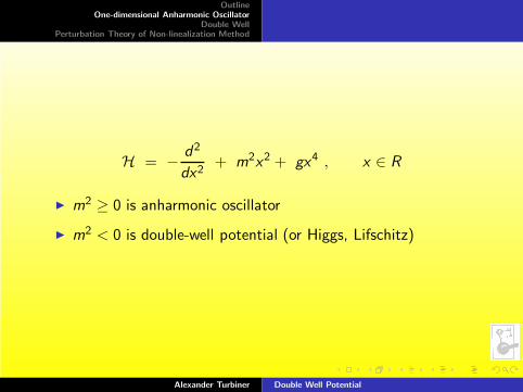
H = − d2

dx2+ m2x2 + gx4 , x ∈ R

◮ m2 ≥ 0 is anharmonic oscillator

◮ m2 < 0 is double-well potential (or Higgs, Lifschitz)




Idea is to combine in a single (approximate) wavefunction:

◮ Perturbation Theory near the minimum of the potential

Ψ(x) = e−αx2(1 + β1x

2 + β2x3 . . .) (ground state)

◮ correct WKB behavior at large distances (inside of the domainof applicability)

◮ Tunneling between classical minima




What is known about eigenfunctions:

◮ For real m2, g ≥ 0 any eigenfunction Ψ(x ; m2, g) is entirefunction in x

◮ Any eigenfunction has finitely many real zeros (theoscillation theorem)

and

infinitely many complex zeros situated on the

imaginary axis

A Eremenko, A Gabrielov (Purdue), B Shapiro(Stockholm), 2008




Take the Schroedinger equation

~2

2µ

d2Ψ

dx2+ (E − V )Ψ = 0

make a formal substitution

Ψ = e−ϕ~

finally,

~dy

dx− y2 = 2µ(E − V ) , y =

dϕ

dx

the Bloch (or Riccati) equation.




Semiclassical expansion

y = y0 + ~y1 + ~2y2 + . . .

y0 = ±(2µ(E − V ))1/2 = ±p , y1 = −1

2log p , etc

Domain of applicability (naive)

~y1

y0≪ 1

Definitely, it is applicable when |p| is large (x → ∞ for growingpotentials)




Main object to study is the logarithmic derivative

y = −Ψ′(x)

Ψ(x)= ϕ′(x) , Ψ(x) = e−ϕ(x)

here ϕ(x) is the phase.




Riccati equation

y ′ − y2 = E − m2x2 − gx4 ,

In general, y is odd and

y = −n∑

i=1

1

x − xi

+ yreg (x)

here xi are nodes and yreg (0) = 0.

Ground state: n = 0 (no nodes), y = yreg

⇒ y has no singularities at real x and y(0) = 0.y(x) = 0 − > extremes of Ψ(x)

If m2 ≥ (m2)crit , ∃ single maximum at x = 0If m2 < (m2)crit , ∃ two maxima and one minimum at x = 0




Asymptotics

Asymptotics:

y = g1/2x |x | + m2

2g1/2

|x |x

+1

x− 4gE + m4

8g3/2

1

x |x | −m2

2g

1

x3+ . . .

|x | → ∞

y = Ex +E 2 − m2

3x3 +

2E (E 2 − m2) − 3g

15x5 + . . .

|x | → 0




Asymptotics

or, for phase

ϕ =g1/2x2|x |

3+

m2

2g1/2|x |+ log |x | − 4gE + m4

8g3/2

1

|x | +m2

g

1

x2+ . . .

|x | → ∞first two terms are H-J asymptotics (classical action), the thirdterm also, but not its coeff is defined (quadratic fluctuations)

ϕ =E

2x2 +

E 2 − m2

12x4 +

2E (E 2 − m2) − 3g

90x6 + . . .

|x | → 0




Interpolation

Let us interpolate perturbation theory at small distances andWKB asymptotics at large distances

ψ0 =1

√

1 + c2gx2exp

{

−A + ax2/2 + bgx4

(D2 + gx2)1/2

}

where A, a, b, c ,D are free (variational) parameters

Very Rigid expression!

(hard to modify)




If we fix

b =1

3, a =

D2

3+ m2 , c =

1

D

then

ψ0 =1

√

D2 + gx2exp

{

−A + (D2 + 3m2)x2/6 + gx4/3

(D2 + gx2)1/2

}

the dominant and the first two subdominant terms in theexpansion of y at |x | → ∞ are reproduced exactly

A,D are still two free parameters which we can vary.

Our approximation has no complex zeroes on imaginary x−axisbut branch cuts going along imaginary axis to ±i∞.




If ψ0 is taken a variational then for all studied m2 from -20 to+20 and g = 2the variational energy reproduces 7 - 10 significant digitscorrectly!!but the accuracy drops down with a decrease of m2 < 0 (from 10to 7 s.d.)




Perturbation Theory and Variational MethodTake a trial function ψ0(x) normalized to 1, then restore thepotential V0, energy E0

ψ′′0 (x)

ψ0(x)= V0 − E0

and construct the Hamiltonian H0 = p2 + V0.

Variational energy

Evar =

∫

ψ0Hψ0 =

∫

ψ0H0 ψ0

︸︷︷︸

=E0

+

∫

ψ0 (H − H0)︸︷︷︸

V−V0

ψ0

︸︷︷︸

=E1

= E0 + E1(V1 = V − V0)




◮ Variational calculations can be considered as the first twoterms in a perturbation theory,it seems natural to require a convergence of this PT series

◮ By calculation of next terms E2,E3, . . . one can evaluate anaccuracy of variational calculation (i) and improve ititeratively (ii)(if the series is convergent, of course)




One more, physical property must be introduced into theapproximation:

at m2 → −∞ the barrier grows, tunneling between wellsdecreases, the wavefunction has two maxima (correspondingto two minima of the potential) and one minimum at originwhich value tends to zero ⇒

ψ0 =1

(D2 + gx2)1/2exp

{

−A + (D2 + 3m2)x2/6 + gx4/3

(D2 + gx2)1/2

}

×

coshαx

(D2 + gx2)1/2

(following the E.M. Lifschitz prescription, Ψ± = Ψ(x + α) ± Ψ(x − α))in total, we have now three free parameters, A,D, α.




With this modification for all studied m2 from -20 to +20 andg = 2

the variational energy reproduces 9 - 11 significant digits

correctly!!




Perturbation Theory of “Non-linealization” Method

Take Riccati equation instead of Schroedinger equation

y ′ − y2 = E − V , y = (log Ψ)′

and develop PT there. If Ψ0 is given, let

V = V0 + λV1

where V0 = Ψ′′0/Ψ0, then perturbation theory

y =∑

λnyn , E =∑

λnEn




For nth correction

λn∣∣∣ y ′

n − 2y0 · yn = En − Qn;

Q1 = V1

Qn = −n−1∑

i=1

yi · yn−i , n = 2, 3, . . .

Multiply both sides by Ψ20,

(Ψ20 yn)

′ = (En − Qn)Ψ20

Boundary condition: |Ψ20 yn| → 0 at |x | → ∞ (no particle current)




En =

∫ ∞

−∞QnΨ

20 dx

∫ ∞

−∞Ψ2

0 dx

yn = Ψ−20

∫ x

−∞

(En − Qn)Ψ20 dx ′

d = 1M. Price (1955), Ya.B. Zel’dovich (1956)

ground-state. . . Y.Aharonov (1979) . . . A.T. (1979) . . .




g = 2 , m2 = 1

D = 4.33441

A = −9.23456

α = 2.74573

* * *

Evar = 1.607541302594

∆Evar = −1.2552 × 10−10

Evar = Evar + ∆Evar = 1.607541302469

all digits are correctthe next correction E3 is of the order of 10−14




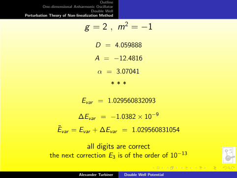
g = 2 , m2 = −1

D = 4.059888

A = −12.4816

α = 3.07041

* * *

Evar = 1.029560832093

∆Evar = −1.0382 × 10−9

Evar = Evar + ∆Evar = 1.029560831054





10

00

1

20

5432

40

30

x

y0

Figure: Logarithmic derivative y0 as function of x for double-wellpotential with m2 = −1, g = 2

32100

−0.001

−0.003

−0.005

54

y1

x

Figure: The first correction y1 for m2 = −1, g = 2




g = 2 , m2 = −20

D = 6.765663

A = −286.6456

α = 49.6136

* * *

Evar = −43.7793127

∆Evar = −3.81 × 10−6

Evar = Evar + ∆Evar = −43.7793165





–5

0

5

10

Yo

15

1 2 3 4

X

Figure: Logarithmic derivative y0 as function of x for double-wellpotential m2 = −20, g = 2




Where d2Ψdx2 |x=0 = 0 ? =⇒ When E = 0 (classical motion

‘stops to feel’ the presence of two minima)

E (m2 = (m2)crit = −3.523390749, g = 2) = 0

◮ for m2 > (m2)crit , d2Ψdx2 |x=0 < 0

(single-peak distribution)For 0 > m2 > (m2)crit the potential is double well one, butwavefunction is single peaked, no memory about two minima,particle prefers to stay near unstable equilibrium point !

◮ for m2 < (m2)crit , d2Ψdx2 |x=0 < 0

(double-peak distribution) as it should be in WKB domain




First Excited State

Similar expansions for |x | → ∞ and x → 0 (with addition− log |x |).

ψ1 =1

(D2 + gx2)exp

{

−A + (D2 + 3m2)x2/6 + gx4/3

(D2 + gx2)1/2

}

×

sinhαx

(D2 + gx2)1/2

(following the E.M.Lifschitz presciption)in total, we have three free parameters, A,D, α.For all studied m2 from -20 to +20 and g = 2 the variationalenergy reproduces 9 - 11 significant digits correctly!!(similar to the ground state)




g = 2 , m2 = −20

D = 5.584375978

A = −246.643750

α = 38.82768

* * *

Evar = −43.77931637

∆Evar = −9.3618 × 10−8

Evar = Evar + ∆Evar = −43.77931646





Energy Gap

∆E = Efirst excited state − Eground state

∆E =211/4

√π

|m2|5/4e−√

2|m2|3/2

6

(

1−71

12

1√2|m2|3/2

−6299

576

1

|m2|3 +. . .

)

at g = 2

J Zinn-Justin et al , 2001




⋆ g = 2 , m2 = −20

∆Evar = 1.03282 × 10−7

∆E(1)var = 1.06529 × 10−7

∆E(2)var = 1.06525 × 10−7

one − instanton = 1.12154 × 10−7 (5.3% deviation)

one − instanton + correction = 1.06908 × 10−7 (0.36% deviation)

one−instanton+twocorrections = 1.06754×10−7 (0.22% deviation)




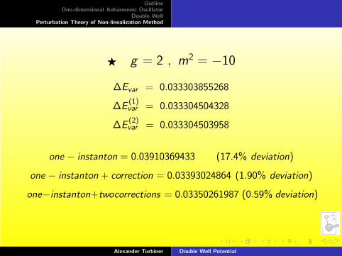
⋆ g = 2 , m2 = −10

∆Evar = 0.033303855268

∆E(1)var = 0.033304504328

∆E(2)var = 0.033304503958

one − instanton = 0.03910369433 (17.4% deviation)

one − instanton + correction = 0.03393024864 (1.90% deviation)

one−instanton+twocorrections = 0.03350261987 (0.59% deviation)




(i) What about excited states ?

(ii) How to modify the function ψ0,1 ?

ψ(k)0 =

Pk(x2)

(D2 + gx2)k+1/2exp

{

−A + ax2/2 + gx4/3

(D2 + gx2)1/2

}

coshαx

(D2 + gx2)1/2

where Pk is a polynomial of kth degree with positive roots foundthrough conditional minimization

(ψ(k)0 , ψ

(ℓ)0 ) = 0 , ℓ = 0, 1, 2, ...(k − 1)




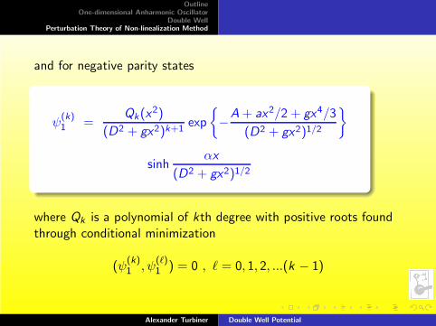
and for negative parity states

ψ(k)1 =

Qk(x2)

(D2 + gx2)k+1exp

{

−A + ax2/2 + gx4/3

(D2 + gx2)1/2

}

sinhαx

(D2 + gx2)1/2

where Qk is a polynomial of kth degree with positive roots foundthrough conditional minimization

(ψ(k)1 , ψ

(ℓ)1 ) = 0 , ℓ = 0, 1, 2, ...(k − 1)




What about sextic oscillator?

H = − d2

dx2+ m2x2 + g4x

4 + g6x6 , x ∈ R

If dimensionless number q ≡ g24

4g3/26

− m2

g1/26

= 2n + 3, n = 0, 1, 2, . . .,

the QES situation occurs, (n + 1) eigenstates are known exactly.♠ For Ground State:

y ′ − y2 = E − m2x2 − g4x4 − g6x

6 , y(0) = 0

y has no simple poles at x ∈ R.




Asymptotics:

y = g1/26 x3 +

g4

2g1/26

x +1

2

(

3 − q

)1

x−

1

2g1/26

[

E +g4

2g1/26

(

1 − q

)]

1

x3+ . . . at |x | → ∞

There is no limit to the quartic osc case when g6 tends to zero!Completely different expansion... But at small distances they aresimilar

y = Ex +E 2 − m2

3x3 +

2E (E 2 − m2) − 3g4

15x5 + . . . at |x | → 0




Asymptotics:

ϕ =g

1/26

4x4 +

g4

4g1/26

x2 +1

2

(

3 − q

)

log x +

1

4g1/26

[

E +g4

2g1/26

(

1 − q

)]

1

x2+ . . . at |x | → ∞

There is no limit to the quartic osc case when g6 tends to zero!For QES case q = 3 (no log term and all subsequent ones).

At small distances

ϕ =E

2x2+

E 2 − m2

12x4+

2E (E 2 − m2) − 3g4

90x6+. . . at |x | → 0




Interpolation:

ψ0 =1

(D2 + 2bx2 + g6x4)3−q

8

exp

{

−A + ax2 + (g4 + b)x4/4 + g6x6/4

(D2 + 2bx2 + g6x4)1/2

}

where A, a, b,D are variational parameters.




If q = 3 the potential is

V = (g24

4g6− 3

√g6)x

2 + g4x4 + g6x

6

and, finally,

ψ0 = exp {− g4

4g1/26

x2 − g1/26

4x4}

It is quasi-exactly-solvable case.




Depending on the parameters the sextic potential has one-, two- orthree minima. The Lifschitz argument leads to

ψ0 =1

(D2 + 2bx2 + g6x4)3−q

8

exp

{

−A + ax2 + (g4 + b)x4/4 + g6x6/4

(D2 + 2bx2 + g6x4)1/2

}

×

coshαx

(D2 + 2bx2 + g6x4)1/2+

B

(D2 + 2bx2 + g6x4)3−q

8

exp

{

− A + ax2 + (g4 + b)x4/4 + g6x6/4

(D2 + 2bx2 + g6x4)1/2

}




Zeeman Effect on Hydrogen

H = −∆ − 2

r+ γ2ρ2 , x ∈ R3

where r =√

x2 + y2 + z2 , ρ =√

x2 + y2 and γ magnetic field.For Ground State:

(∇ · ~y) − ~y2 = E − V , ~y = ∇ log Ψ




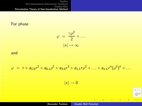
For phase

ϕ =γρ2

2+ . . .

|x | → ∞and

ϕ = r + a2,0r2 + a0,1ρ

2 + a3,0r3 + a1,1rρ

2 + . . .+ an,k rn(ρ2)k + . . .

|x | → 0




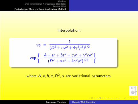
Interpolation:

ψ0 =1

(D2 + αz2 + 4γ2ρ2)1/2

exp

{

−A + ar + bz2 + cρ2 + γ2rρ2

(D2 + αz2 + 4γ2ρ2)1/2

}

where A, a, b, c ,D2, α are variational parameters.




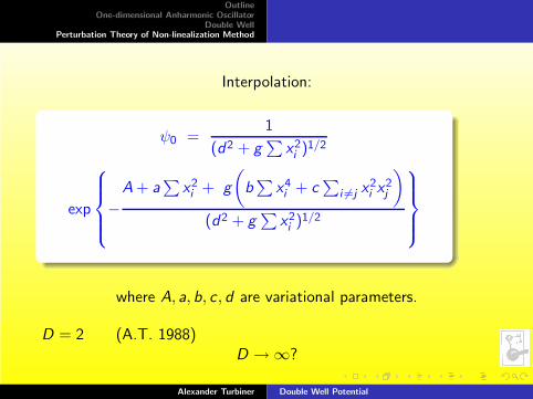
What about multidimensional quartic oscillator?

H = −∆ + m2∑

x2i + g

(∑

x4i + c

∑

i 6=j

x2i x2

j

)

≡ −∆ + V ,

in x ∈ RD .For Ground State:

(∇ · ~y) − ~y2 = E − V , ~y = ∇ log Ψ




Interpolation:

ψ0 =1

(d2 + g∑

x2i )1/2

exp

−A + a

∑x2i + g

(

b∑

x4i + c

∑

i 6=j x2i x2

j

)

(d2 + g∑

x2i )1/2

where A, a, b, c , d are variational parameters.

D = 2 (A.T. 1988)D → ∞?


Double Well Potential: Perturbation Theory, [10pt ...

Documents

Transcript of Double Well Potential: Perturbation Theory, [10pt ...