Dottorato in Informatica, Sistemi e Telecomunicazioni … degli Studi di Firenze` Dottorato in...
163
Universit` a degli Studi di Firenze Dottorato in Informatica, Sistemi e Telecomunicazioni Indirizzo: Ingegneria Informatica e dell’Automazione Ciclo XXVII Coordinatore: Prof. Luigi Chisci Distributed multi-object tracking over sensor networks: a random finite set approach Dipartimento di Ingegneria dell’Informazione Settore Scientifico Disciplinare ING-INF/04 Author: Claudio Fantacci Supervisors: Prof. Luigi Chisci Prof. Giorgio Battistelli Coordinator: Prof. Luigi Chisci Years 2012/2014 arXiv:1508.04158v1 [stat.ME] 12 Jul 2015
Transcript of Dottorato in Informatica, Sistemi e Telecomunicazioni … degli Studi di Firenze` Dottorato in...

Universita degli Studi di Firenze
Dottorato in Informatica, Sistemi e TelecomunicazioniIndirizzo: Ingegneria Informatica e dell’Automazione
Ciclo XXVIICoordinatore: Prof. Luigi Chisci
Distributed multi-object trackingover sensor networks:
a random finite set approach
Dipartimento di Ingegneria dell’InformazioneSettore Scientifico Disciplinare ING-INF/04
Author:
Claudio Fantacci
Supervisors:
Prof. Luigi Chisci
Prof. Giorgio Battistelli
Coordinator:
Prof. Luigi Chisci
Years 2012/2014
arX
iv:1
508.
0415
8v1
[st
at.M
E]
12
Jul 2
015


Contents
Acknowledgment 1
Foreword 3
Abstract 5
1 Introduction 7
2 Background 132.1 Network model . . . . . . . . . . . . . . . . . . . . . . . . . . . . . . . . . . . 132.2 Recursive Bayesian estimation . . . . . . . . . . . . . . . . . . . . . . . . . . . 15
2.2.1 Notation . . . . . . . . . . . . . . . . . . . . . . . . . . . . . . . . . . . 152.2.2 Bayes filter . . . . . . . . . . . . . . . . . . . . . . . . . . . . . . . . . 152.2.3 Kalman Filter . . . . . . . . . . . . . . . . . . . . . . . . . . . . . . . . 172.2.4 The Extended Kalman Filter . . . . . . . . . . . . . . . . . . . . . . . 192.2.5 The Unscented Kalman Filter . . . . . . . . . . . . . . . . . . . . . . . 20
2.3 Random finite set approach . . . . . . . . . . . . . . . . . . . . . . . . . . . . 222.3.1 Notation . . . . . . . . . . . . . . . . . . . . . . . . . . . . . . . . . . . 232.3.2 Random finite sets . . . . . . . . . . . . . . . . . . . . . . . . . . . . . 232.3.3 Common classes of RFS . . . . . . . . . . . . . . . . . . . . . . . . . . 262.3.4 Bayesian multi-object filtering . . . . . . . . . . . . . . . . . . . . . . . 282.3.5 CPHD filtering . . . . . . . . . . . . . . . . . . . . . . . . . . . . . . . 302.3.6 Labeled RFSs . . . . . . . . . . . . . . . . . . . . . . . . . . . . . . . . 312.3.7 Common classes of labeled RFS . . . . . . . . . . . . . . . . . . . . . . 322.3.8 Bayesian multi-object tracking . . . . . . . . . . . . . . . . . . . . . . 36
2.4 Distributed information fusion . . . . . . . . . . . . . . . . . . . . . . . . . . 382.4.1 Notation . . . . . . . . . . . . . . . . . . . . . . . . . . . . . . . . . . . 392.4.2 Kullback-Leibler average of PDFs . . . . . . . . . . . . . . . . . . . . . 392.4.3 Consensus algorithms . . . . . . . . . . . . . . . . . . . . . . . . . . . 402.4.4 Consensus on posteriors . . . . . . . . . . . . . . . . . . . . . . . . . . 41
I

3 Distributed single-object filtering 453.1 Consensus-based distributed filtering . . . . . . . . . . . . . . . . . . . . . . . 45
3.1.1 Parallel consensus on likelihoods and priors . . . . . . . . . . . . . . . 453.1.2 Approximate CLCP . . . . . . . . . . . . . . . . . . . . . . . . . . . . 483.1.3 A tracking case-study . . . . . . . . . . . . . . . . . . . . . . . . . . . 50
3.2 Consensus-based distributed multiple-model filtering . . . . . . . . . . . . . . 513.2.1 Notation . . . . . . . . . . . . . . . . . . . . . . . . . . . . . . . . . . . 523.2.2 Bayesian multiple-model filtering . . . . . . . . . . . . . . . . . . . . . 523.2.3 Networked multiple model estimation via consensus . . . . . . . . . . 543.2.4 Distributed multiple-model algorithms . . . . . . . . . . . . . . . . . . 553.2.5 Connection with existing approach . . . . . . . . . . . . . . . . . . . . 563.2.6 A tracking case-study . . . . . . . . . . . . . . . . . . . . . . . . . . . 58
4 Distributed multi-object filtering 694.1 Multi-object information fusion via consensus . . . . . . . . . . . . . . . . . . 69
4.1.1 Multi-object Kullback-Leibler average . . . . . . . . . . . . . . . . . . 704.1.2 Consensus-based multi-object filtering . . . . . . . . . . . . . . . . . . 714.1.3 Connection with existing approaches . . . . . . . . . . . . . . . . . . . 724.1.4 CPHD fusion . . . . . . . . . . . . . . . . . . . . . . . . . . . . . . . . 73
4.2 Consensus GM-CPHD filter . . . . . . . . . . . . . . . . . . . . . . . . . . . . 764.3 Performance evaluation . . . . . . . . . . . . . . . . . . . . . . . . . . . . . . 79
5 Centralized multi-object tracking 875.1 The δ-GLMB filter . . . . . . . . . . . . . . . . . . . . . . . . . . . . . . . . . 88
5.1.1 δ-GLMB prediction . . . . . . . . . . . . . . . . . . . . . . . . . . . . 885.1.2 δ-GLMB update . . . . . . . . . . . . . . . . . . . . . . . . . . . . . . 89
5.2 GLMB approximation of multi-object densities . . . . . . . . . . . . . . . . . 905.3 Marginalizations of the δ-GLMB density . . . . . . . . . . . . . . . . . . . . . 915.4 The Mδ-GLMB filter . . . . . . . . . . . . . . . . . . . . . . . . . . . . . . . . 92
5.4.1 Mδ-GLMB prediction . . . . . . . . . . . . . . . . . . . . . . . . . . . 925.4.2 Mδ-GLMB update . . . . . . . . . . . . . . . . . . . . . . . . . . . . . 93
5.5 The LMB filter . . . . . . . . . . . . . . . . . . . . . . . . . . . . . . . . . . . 955.5.1 Alternative derivation of the LMB Filter . . . . . . . . . . . . . . . . . 955.5.2 LMB prediction . . . . . . . . . . . . . . . . . . . . . . . . . . . . . . . 965.5.3 LMB update . . . . . . . . . . . . . . . . . . . . . . . . . . . . . . . . 97
5.6 Performance evaluation . . . . . . . . . . . . . . . . . . . . . . . . . . . . . . 985.6.1 Scenario 1: radar . . . . . . . . . . . . . . . . . . . . . . . . . . . . . . 1015.6.2 Scenario 2: 3 TOA sensors . . . . . . . . . . . . . . . . . . . . . . . . 101

6 Distributed multi-object tracking 1076.1 Information fusion with labeled RFS . . . . . . . . . . . . . . . . . . . . . . . 108
6.1.1 Labeled multi-object Kullback-Leibler average . . . . . . . . . . . . . 1086.1.2 Normalized weighted geometric mean of Mδ-GLMB densities . . . . . 1096.1.3 Normalized weighted geometric mean of LMB densities . . . . . . . . 1106.1.4 Distributed Bayesian multi-object tracking via consensus . . . . . . . 111
6.2 Consensus labeled RFS information fusion . . . . . . . . . . . . . . . . . . . . 1126.2.1 Consensus Mδ-GLMB filter . . . . . . . . . . . . . . . . . . . . . . . . 1126.2.2 Consensus LMB filter . . . . . . . . . . . . . . . . . . . . . . . . . . . 113
6.3 Performance evaluation . . . . . . . . . . . . . . . . . . . . . . . . . . . . . . 1146.3.1 High SNR . . . . . . . . . . . . . . . . . . . . . . . . . . . . . . . . . . 1186.3.2 Low SNR . . . . . . . . . . . . . . . . . . . . . . . . . . . . . . . . . . 1186.3.3 Low PD . . . . . . . . . . . . . . . . . . . . . . . . . . . . . . . . . . . 119
7 Conclusions and future work 123
A Proofs 127Proof of Theorem 1 . . . . . . . . . . . . . . . . . . . . . . . . . . . . . . . . . . . . 127Proof of Theorem 2 . . . . . . . . . . . . . . . . . . . . . . . . . . . . . . . . . . . . 128Proof of Proposition 1 . . . . . . . . . . . . . . . . . . . . . . . . . . . . . . . . . . 128Proof of Proposition 2 . . . . . . . . . . . . . . . . . . . . . . . . . . . . . . . . . . 130Proof of Theorem 4 . . . . . . . . . . . . . . . . . . . . . . . . . . . . . . . . . . . . 132Proof of Proposition 3 . . . . . . . . . . . . . . . . . . . . . . . . . . . . . . . . . . 133Proof of Lemma 1 . . . . . . . . . . . . . . . . . . . . . . . . . . . . . . . . . . . . 133Proof of Theorem 5 . . . . . . . . . . . . . . . . . . . . . . . . . . . . . . . . . . . . 133Proof of Proposition 4 . . . . . . . . . . . . . . . . . . . . . . . . . . . . . . . . . . 134
Bibliography 135


List of Theorems andPropositions
1 Theorem (KLA of PMFs) . . . . . . . . . . . . . . . . . . . . . . . . . . . . . 54
2 Theorem (Multi-object KLA) . . . . . . . . . . . . . . . . . . . . . . . . . . . 71
1 Proposition (GLMB approximation) . . . . . . . . . . . . . . . . . . . . . . . 912 Proposition (The Mδ-GLMB density) . . . . . . . . . . . . . . . . . . . . . . 92
3 Theorem (KLA of labeled RFSs) . . . . . . . . . . . . . . . . . . . . . . . . . 1094 Theorem (NWGM of Mδ-GLMB RFSs) . . . . . . . . . . . . . . . . . . . . . 1093 Proposition (KLA of Mδ-GLMB RFSs) . . . . . . . . . . . . . . . . . . . . . 1095 Theorem (NWGM of LMB RFSs) . . . . . . . . . . . . . . . . . . . . . . . . . 1104 Proposition (KLA of LMB RFSs) . . . . . . . . . . . . . . . . . . . . . . . . . 1101 Lemma (Normalization constant of LMB KLA) . . . . . . . . . . . . . . . . . 133
V


List of Figures
2.1 Network model . . . . . . . . . . . . . . . . . . . . . . . . . . . . . . . . . . . 14
3.1 Network and object trajectory. . . . . . . . . . . . . . . . . . . . . . . . . . . 503.2 Object trajectory considered in the simulation experiments . . . . . . . . . . 593.3 Network with 4 DOA, 4 TOA sensors and 4 communication nodes. . . . . . . 603.4 Estimated object trajectories of node 1 (TOA, green dash-dotted line) and
node 2 (TOA, red dashed line) in the sensor network of fig. 3.3. The realobject trajectory is the blue continuous line. . . . . . . . . . . . . . . . . . . . 61
4.1 Network with 7 sensors: 4 TOA and 3 DOA. . . . . . . . . . . . . . . . . . . 804.2 object trajectories considered in the simulation experiment. The start/end
point for each trajectory is denoted, respectively, by •\. . . . . . . . . . . . 814.3 Borderline position GM initialization. The symbol denotes the component
mean while the blue solid line and the red dashed line are, respectively, their3σ and 2σ confidence regions. . . . . . . . . . . . . . . . . . . . . . . . . . . . 82
4.4 Cardinality statistics for GGM-CPHD. . . . . . . . . . . . . . . . . . . . . . . 834.5 Cardinality statistics for CGM-CPHD with L = 1 consensus step. . . . . . . . 834.6 Cardinality statistics for CGM-CPHD with L = 2 consensus steps. . . . . . . 844.7 Cardinality statistics for CGM-CPHD with L = 3 consensus steps. . . . . . . 844.8 Performance comparison, using OSPA, between GGM-CPHD and CGM-CPHD
respectively with L = 1, L = 2 and L = 3 consensus steps. . . . . . . . . . . . 854.9 GM representation within TOA sensor 1 (see Fig. 2) at the initial time instant
throughout the consensus process. Means and 99.7% confidence ellipses of theGaussian components of the location PDF are displayed in the horizontal planewhile weights of such components are on the vertical axis. . . . . . . . . . . . 86
5.1 Network with 3 TOA sensors. . . . . . . . . . . . . . . . . . . . . . . . . . . . 995.2 Object trajectories considered in the simulation experiment. The start/end
point for each trajectory is denoted, respectively, by •\. The ? indicates arendezvous point. . . . . . . . . . . . . . . . . . . . . . . . . . . . . . . . . . . 100
5.3 Cardinality statistics for Mδ-GLMB tracking filter using 1 radar. . . . . . . . 102
VII

5.4 Cardinality statistics for δ-GLMB tracking filter using 1 radar. . . . . . . . . 1025.5 Cardinality statistics for LMB tracking filter using 1 radar. . . . . . . . . . . 1035.6 OSPA distance (c = 600 [m], p = 2) using 1 radar. . . . . . . . . . . . . . . . 1035.7 Cardinality statistics for Mδ-GLMB tracking filter using 3 TOA. . . . . . . . 1045.8 Cardinality statistics for δ-GLMB tracking filter using 3 TOA. . . . . . . . . 1045.9 Cardinality statistics for LMB tracking filter using 3 TOA. . . . . . . . . . . 1055.10 OSPA distance (c = 600 [m], p = 2) using 3 TOA. . . . . . . . . . . . . . . . . 105
6.1 Network with 7 sensors: 4 TOA and 3 DOA. . . . . . . . . . . . . . . . . . . 1156.2 Tbject trajectories considered in the simulation experiment. The start/end
point for each trajectory is denoted, respectively, by •\. The ? indicates arendezvous point. . . . . . . . . . . . . . . . . . . . . . . . . . . . . . . . . . . 116
6.3 Cardinality statistics for the GM-CCPHD filter under high SNR. . . . . . . . 1196.4 Cardinality statistics for the GM-CLMB tracker under high SNR. . . . . . . . 1196.5 Cardinality statistics for the GM-CMδGLMB tracker under high SNR. . . . . 1206.6 OSPA distance (c = 600 [m], p = 2) under high SNR. . . . . . . . . . . . . . . 1206.7 Cardinality statistics for the GM-CCPHD filter under low SNR. . . . . . . . . 1216.8 Cardinality statistics for the GM-CMδGLMB tracker under low SNR. . . . . 1216.9 OSPA distance (c = 600 [m], p = 2) under low SNR. . . . . . . . . . . . . . . 1216.10 Cardinality statistics for the GM-CMδGLMB tracker under low PD. . . . . . 1226.11 OSPA distance (c = 600 [m], p = 2) under low PD. . . . . . . . . . . . . . . . 122

List of Tables
2.1 The Kalman Filter (KF) . . . . . . . . . . . . . . . . . . . . . . . . . . . . . . 182.2 The Multi-Sensor Kalman Filter (MSKF) . . . . . . . . . . . . . . . . . . . . 192.3 The Extended Kalman Filter (EKF) . . . . . . . . . . . . . . . . . . . . . . . 202.4 The Unscented Transformation (UT) . . . . . . . . . . . . . . . . . . . . . . . 212.5 Unscented Transformation Weights (UTW) . . . . . . . . . . . . . . . . . . . 212.6 The Unscented Kalman Filter (UKF) . . . . . . . . . . . . . . . . . . . . . . . 222.7 Sampling a Poisson RFS . . . . . . . . . . . . . . . . . . . . . . . . . . . . . . 272.8 Sampling an i.i.d. RFS . . . . . . . . . . . . . . . . . . . . . . . . . . . . . . . 282.9 Sampling a multi-Bernoulli RFS . . . . . . . . . . . . . . . . . . . . . . . . . 292.10 Sampling a labeled Poisson RFS . . . . . . . . . . . . . . . . . . . . . . . . . 322.11 Sampling a labeled i.i.d. cluster RFS . . . . . . . . . . . . . . . . . . . . . . . 332.12 Sampling a labeled multi-Bernoulli RFS . . . . . . . . . . . . . . . . . . . . . 362.13 Consensus on Posteriors (CP) . . . . . . . . . . . . . . . . . . . . . . . . . . . 43
3.1 Consensus on Likelihoods and Priors (CLCP) pseudo-code . . . . . . . . . . . 463.2 Analytical implementation of Consensus on Likelihoods and Priors (CLCP) . 493.3 Performance comparison . . . . . . . . . . . . . . . . . . . . . . . . . . . . . . 513.4 Centralized Bayesian Multiple-Model (CBMM) filter pseudo-code . . . . . . . 623.5 Centralized First-Order Generalized Pseudo-Bayesian (CGBP1) filter pseudo-
code . . . . . . . . . . . . . . . . . . . . . . . . . . . . . . . . . . . . . . . . . 633.6 Centralized Interacting Multiple Model (CIMM) filter pseudo-code . . . . . . 643.7 Distributed GPB1 (DGPB1) filter pseudo-code . . . . . . . . . . . . . . . . . 653.8 Distributed IMM (DIMM) filter pseudo-code . . . . . . . . . . . . . . . . . . 663.9 Performance comparison for the sensor network of fig. 3.3 . . . . . . . . . . . 67
4.1 Distributed GM-CPHD (DGM-CPHD) filter pseudo-code . . . . . . . . . . . 774.2 Merging pseudo-code . . . . . . . . . . . . . . . . . . . . . . . . . . . . . . . . 784.3 Pruning pseudo-code . . . . . . . . . . . . . . . . . . . . . . . . . . . . . . . . 784.4 Estimate extraction pseudo-code . . . . . . . . . . . . . . . . . . . . . . . . . 794.5 Number of Gaussian components before consensus for CGM-CPHD . . . . . . 85
IX

5.1 Components of the LMB RFS birth process at a given time k. . . . . . . . . . 100
6.1 Gaussian Mixture - Consensus Marginalized δ-Generalized Labeled Multi-Bernoulli(GM-CMδGLMB) filter . . . . . . . . . . . . . . . . . . . . . . . . . . . . . . 113
6.2 GM-CMδGLMB estimate extraction . . . . . . . . . . . . . . . . . . . . . . . 1136.3 Gaussian Mixture - Consensus Labeled Multi-Bernoulli (GM-CLMB) filter . . 1146.4 GM-CLMB estimate extraction . . . . . . . . . . . . . . . . . . . . . . . . . . 1156.5 Components of the LMB RFS birth process at a given time k. . . . . . . . . . 117

List of Acronyms
BF Bayes FilterBMF Belief Mass FunctionCBMM Centralized Bayesian Multiple-ModelCDF Cumulative Distribution FunctionCI Covariance IntersectionCMδGLMB Consensus Marginalized δ-Generalized Labelled Multi-BernoulliCGM-CPHD Consensus Gaussian Mixture-Cardinalized Probability
Hypothesis DensityCLCP Consensus on Likelihoods and PriorsCLMB Consensus Labelled Multi-BernoulliCOM CommunicationCP Consensus on PosteriorsCPHD Cardinalized Probability Hypothesis DensityCT Coordinated Turnδ-GLMB δ-Generalized Labeled Multi-BernoulliDGPB1 Distributed First Order Generalized Pseudo-BayesianDIMM Distributed Interacting Multiple ModelDIMM-CL Distributed Interacting Multiple Model with Consensus on
LikelihoodsDMOF Distributed Multi-Object FilteringDMOT Distributed Multi-Object TrackingDOA Direction Of ArrivalDSOF Distributed Single-Object FilteringDWNA Discrete White Noise AccelerationEKF Extended Kalman FilterEMD Exponential Mixture DensityFISST FInite Set STatisticsGCI Generalized Covariance Intersection
XI

GGM-CPHD Global Gaussian Mixture - Cardinalized Probability HypothesisDensity
GLMB Generalized Labeled Multi-BernoulliGM Gaussian MixtureGM-CMδGLMB Gaussian Mixture-Consensus Marginalized δ-Generalized
Labelled Multi-BernoulliGM-CLMB Gaussian Mixture-Consensus Labelled Multi-BernoulliGM-δGLMB Gaussian Mixture-δ-Generalized Labelled Multi-BernoulliGM-LMB Gaussian Mixture-Labelled Multi-BernoulliGM-MδGLMB Gaussian Mixture-Marginalized δ-Generalized Labelled
Multi-BernoulliGPB1 First Order Generalized Pseudo-BayesianI.I.D. / i.i.d. / iid Independent and Identically DistributedIMM Interacting Multiple ModelJPDA Joint Probabilistic Data AssociationKF Kalman FilterKLA Kullback-Leibler AverageKLD Kullback-Leibler DivergenceLMB Labeled Multi-BernoulliMδ-GLMB Marginalized δ-Generalized Labelled Multi-BernoulliMHT Multiple Hypotheses TrackingMM Multiple ModelMOF Multi-Object FilteringMOT Multi-Object TrackingMSKF Multi-Sensor Kalman FilterNCV Nearly-Constant VelocityNWGM Normalized Weighted Geometric MeanOSPA Optimal SubPattern AssignmentOT Object TrackingPF Particle FilterPDF Probability Density FunctionPHD Probability Hypothesis DensityPMF Probability Mass FunctionPRMSE Position Root Mean Square ErrorRFS Random Finite SetSEN SensorSMC Sequential Monte CarloSOF Single-Object Filtering

TOA Time Of ArrivalUKF Unscented Kalman FilterUT Unscented Transform

List of Symbols
G Directed graphN Set of nodesA Set of arcsS Set of sensorsC Set of communication nodesN j Set of in-neighbours (including j itself)col(·i)i∈I Stacking operator
diag(·i)i∈I Square diagonal matrix operator
〈f, g〉 ,∫f(x) g(x)dx Inner product operator for vector valued functions
> Transpose operatorR Real number spaceRn n dimensional Euclidean spaceN Natural number setk Time indexxk State vectorX State spacenx Dimension of the state vectorfk(x) State transition functionwk Process noiseϕ(k|ζ) Markov transition densityyk Measurement vectorY Measurement spaceny Dimension of the measurement vectorhk(x) Measurement functionvk Measurement noisegk(y|x) Likelihood functionx1:k State historyy1:k Measurement history
XV

pk(x) Posterior/Filtered probability density functionpk|k−1(x) Prior/Predicted probability density functionp0(x) Initial probability density functiongik (y|x) Likelihood function of sensor iAk−1 nx × nx state transition matrixCk ny × nx observation matrixQk Process noise covariance matrixRk Measurement noise covariance matrixN (·; ·, ·) Gaussian probability density functionxk Updated mean (state vector)Pk Updated covariance matrix (associated to xk)xk|k−1 Predicted mean (state vector)Pk|k−1 Predicted covariance matrix (associated to xk|k−1)ek InnovationSk Innovation covariance matrixKk Kalman gainασ, βσ, κσ Unscented transformation weights parametersc, wm, wc, Wc Unscented transformation weightsX Finite-valued-sethX ,
∏x∈X
h(x) Multi-object exponential
δX(·) Generalized Kronecker delta1X(·) Generalized indicator function| · | Cardinality operatorF(X) Space of finite subsets of XFn(X) Space of finite subsets of X with exactly n elementsf(X), π(X) Multi-object densitiesρ(n) Cardinality probability mass functionβ(X) Belief mass functiond(x) Probability hypothesis density functionE[ · ] Expectation operatorn, D Expected number of objectss(x) Location density (normalized d(x))r Bernoulli existence probabilityq , 1− r Bernoulli non-existence probabilityXk Multi-object random finite setYk Random finite set of the observationsY1:k Observation history random finite set

Y ik Random finite set of the observations of sensor iBk Random finite set of new-born objectsPS,k Survival probabilityC, Ck Random finite sets of clutterCi, Cik Random finite sets of clutter of sensor iPD,k Detection probabilityπk(X) Posterior/Filtered multi-object densityπk|k−1(X) Prior/Predicted multi-object densityϕk|k−1(X|Z) Markov multi-object transition densitygk(Y |X) Multi-object likelihood functionρk|k−1(n) Predicted cardinality probability mass functiondk|k−1(x) Predicted probability hypothesis density functionρk(n) Updated cardinality probability mass functiondk(x) Updated probability hypothesis density functionpb,k(·) Birth cardinality probability mass functionρS,k|k−1(·) Cardinality probability mass function of survived objectsdb,k(·) Probability hypothesis density function of new-born objectsG0k(·, ·, ·), GYk
(·) Cardinalized probability hypothesis density function generalizedlikelihood functions
` LabelX Labeled finite-valued-setx Labeled state vectorL(X) Label projection operator∆(X) Distinct label indicatorLk, B Label set for objects born at time kL1:k−1, L− Label set for objects up to time k − 1L1:k, L Label set for objects up to time kξ Association historyΞ Association history setf(X), π(X) Labeled multi-object densitiesw(c), w(c)(X) Generalized labeled multi-Bernoulli weights indexed with c ∈ Cp(c) Generalized labeled multi-Bernoulli location probability density
function indexed with c ∈ C(I, ξ) ∈ F(L)× Ξ Labeled multi-object hypothesisw(I,ξ)(X) δ-Generalized labeled multi-Bernoulli weight of hypothesis (I, ξ)p(I) δ-Generalized labeled multi-Bernoulli location probability density
function with association history ξ

r(`) Bernoulli existence probability associated to the object with label`
q(`) Bernoulli non-existence probability associated to the object withlabel `
ϕk|k−1(X|Z) Markov labeled multi-object transition density
(p⊕ q) (x) , p(x) q(x)〈p, q〉
Information fusion operator
(α p) (x) , [p(x)]α
〈pα, 1〉 Information weighting operator
p(x), q, f , . . . Weighted Kullback-Leibler average(q,Ω) Information vector and (inverse covariance) matrixωi,j Consensus weight of node i relative to jωi,jl Consensus weight of node i relative to j at the consensus step l
Π Consensus matrixl Consensus stepL Maximum number of consensus stepsρi Likelihood scalar weight of node ibi Estimate of the fraction |S/N|δΩi
k ,(Cik)> (
Rik)−1
Cik Information matrix gainδqik ,
(Cik)> (
Rik)−1
yik Information vector gainPc Sets of probability density functions over a continuous state spacePd Sets of probability mass functions over a discrete state spacepjt Markov transition probability from mode t to jµjk Filtered modal probability of mode jµjk|k−1 Predicted modal probability of mode jµj|tk Filtered modal probability of mode j conditioned to mode tαi Gaussian mixture weight of the component iNG Number of components of a Gaussian mixtureαij Fused Gaussian mixture weight relative to components i and j
Ts Sampling intervalβ Fused Gaussian mixture normalizing constantpx, py Object planar position coordinatespx, py Object planar velocity coordinatesλc Poisson clutter rateNmc Number of Monte Carlo trialsNmax Maximum number of Gaussian componentsγm Merging thresholdγt Truncation thresholdσTOA Standard deviation of time of arrival sensor

σDOA Standard deviation of direction of arrival sensorπk(X) Posterior/Filtered labeled multi-object densityπk|k−1(X) Prior/Predicted labeled multi-object densityfB(X) Labeled multi-object birth densitywB (X) Labeled multi-object birth weightpB(x, `) Labeled multi-object birth location probability density functionr
(`)B Labeled multi-Bernoulli newborn object weightp
(`)B (x) Labeled multi-Bernoulli newborn object location probability den-
sity functionw
(ξ)S (X) Labeled multi-object survival object weight with association his-
tory ξpS(x, `) Labeled multi-object survival object location probability density
function with association history ξθ New association mapΘ(I) New association map set corresponding to the label subset Iw
(I,ξ)k δ-Generalized labeled multi-Bernoulli posterior/filtered weight of
hypothesis (I, ξ)p
(ξ)k (x, `) δ-Generalized labeled multi-Bernoulli posterior/filtered location
probability density function with association history ξw
(I,ξ)k|k−1 δ-Generalized labeled multi-Bernoulli prior/predicted weight of
hypothesis (I, ξ)p
(ξ)k|k−1(x, `) δ-Generalized labeled multi-Bernoulli prior/predicted location
probability density function with association history ξ and label`
w(I)k Marginalized δ-Generalized labeled multi-Bernoulli poste-
rior/filtered weight of the set Ip
(I)k (x, `) Marginalized δ-Generalized labeled multi-Bernoulli poste-
rior/filtered location probability density function of the set Iand label `
w(I)k|k−1 Marginalized δ-Generalized labeled multi-Bernoulli
prior/predicted weight of the set Ip
(I)k|k−1(x, `) Marginalized δ-Generalized labeled multi-Bernoulli
prior/predicted location probability density function of theset I and label `
r(`)S Labeled multi-Bernoulli survival object weightp
(`)S (x) Labeled multi-Bernoulli survival object location probability den-
sity functionr
(`)k Labeled multi-Bernoulli posterior/filtered existence probability of
the object with label `p
(`)k (x) Labeled multi-Bernoulli posterior/filtered location probability
density function of the object with label `
r(`)k|k−1 Labeled multi-Bernoulli prior/predicted existence probability of
the object with label `p
(`)k|k−1(x) Labeled multi-Bernoulli prior/predicted location probability den-
sity function of the object with label `
〈f, g〉 ,∫f(X) g(X)δX Inner product operator for finite-valued-set functions
〈f ,g〉 ,∫
f(X) g(X)δX Inner product operator for labeled finite-valued-set functions

Acknowledgment
First and foremost, I would sincerely like to thank my supervisors Prof. Luigi Chisci andProf. Giorgio Battistelli for their constant and relentless support and guidance during my3-year doctorate. Their invaluable teaching and enthusiasm for research have made my Ph.D.education a very challenging yet rewarding experience. I would also like to thank Dr. AlfonsoFarina, Prof. Ba-Ngu Vo and Prof. Ba-Tuong Vo. It has been a sincere pleasure to have theopportunity to work with such passionate, stimulating and friendly people. Our collaboration,knowledge sharing and feedback have been of great help and truly appreciated. Last but notleast, I would like to thank all my friends and my family who supported, helped and inspiredme during my studies.
1


Foreword
Statistics, mathematics and computer science have always been the favourite subjects in myacademic career. The Ph.D. in automation and computer science engineering brought me toaddress challenging problems involving such disciplines. In particular, multi-object filteringconcerns the joint detection and estimation of an unknown and possibly time-varying numberof objects, along with their dynamic states, given a sequence of observation sets. Further,its distributed formulation also considers how to efficiently address such a problem over aheterogeneous sensor network in a fully distributed, scalable and computationally efficientway. Distributed multi-object filtering is strongly linked with statistics and mathematicsfor modeling and tackling the main issues in an elegant and rigorous way, while computerscience is fundamental for implementing and testing the resulting algorithms. This topicposes significant challenges and is indeed an interesting area of research which has fascinatedme during the whole Ph.D. period.
This thesis is the result of the research work carried out at the University of Florence(Florence, Italy) during the years 2012-2014, of a scientific collaboration for the biennium2012-2013 with Selex ES (former SELEX SI, Rome, Italy) and of 6 months spent as a visitingPh.D. scholar at the Curtin University of Technology (Perth, Australia) during the periodJanuary-July 2014.
3


Abstract
The aim of the present dissertation is to address distributed tracking over a network of het-erogeneous and geographically dispersed nodes (or agents) with sensing, communication andprocessing capabilities. Tracking is carried out in the Bayesian framework and its extensionto a distributed context is made possible via an information-theoretic approach to data fusionwhich exploits consensus algorithms and the notion of Kullback–Leibler Average (KLA) ofthe Probability Density Functions (PDFs) to be fused.
The first step toward distributed tracking considers a single moving object. Consensustakes place in each agent for spreading information over the network so that each node cantrack the object. To achieve such a goal, consensus is carried out on the local single-objectposterior distribution, which is the result of local data processing, in the Bayesian setting,exploiting the last available measurement about the object. Such an approach is calledConsensus on Posteriors (CP). The first contribution of the present work [BCF14a] is animprovement to the CP algorithm, namely Parallel Consensus on Likelihoods and Priors(CLCP). The idea is to carry out, in parallel, a separate consensus for the novel information(likelihoods) and one for the prior information (priors). This parallel procedure is conceivedto avoid underweighting the novel information during the fusion steps. The outcomes of thetwo consensuses are then combined to provide the fused posterior density. Furthermore, thecase of a single highly-maneuvering object is addressed. To this end, the object is modeledas a jump Markovian system and the multiple model (MM) filtering approach is adopted forlocal estimation. Thus, the consensus algorithms needs to be re-designed to cope with thisnew scenario. The second contribution [BCF+14b] has been to devise two novel consensusMM filters to be used for tracking a maneuvering object. The novel consensus-based MMfilters are based on the First Order Generalized Pseudo-Bayesian (GPB1) and InteractingMultiple Model (IMM) filters.
The next step is in the direction of distributed estimation of multiple moving objects.In order to model, in a rigorous and elegant way, a possibly time-varying number of objectspresent in a given area of interest, the Random Finite Set (RFS) formulation is adopted sinceit provides the notion of probability density for multi-object states that allows to directly ex-tend existing tools in distributed estimation to multi-object tracking. The multi-object Bayesfilter proposed by Mahler is a theoretically grounded solution to recursive Bayesian trackingbased on RFSs. However, the multi-object Bayes recursion, unlike the single-object coun-
5

terpart, is affected by combinatorial complexity and is, therefore, computationally infeasibleexcept for very small-scale problems involving few objects and/or measurements. For this rea-son, the computationally tractable Probability Hypothesis Density (PHD) and CardinalizedPHD (CPHD) filtering approaches will be used as a first endeavour to distributed multi-object filtering. The third contribution [BCF+13a] is the generalisation of the single-objectKLA to the RFS framework, which is the theoretical fundamental step for developing a novelconsensus algorithm based on CPHD filtering, namely the Consensus CPHD (CCPHD). Eachtracking agent locally updates multi-object CPHD, i.e. the cardinality distribution and thePHD, exploiting the multi-object dynamics and the available local measurements, exchangessuch information with communicating agents and then carries out a fusion step to combinethe information from all neighboring agents.
The last theoretical step of the present dissertation is toward distributed filtering withthe further requirement of unique object identities. To this end the labeled RFS frameworkis adopted as it provides a tractable approach to the multi-object Bayesian recursion. The δ-GLMB filter is an exact closed-form solution to the multi-object Bayes recursion which jointlyyields state and label (or trajectory) estimates in the presence of clutter, misdetections and as-sociation uncertainty. Due to the presence of explicit data associations in the δ-GLMB filter,the number of components in the posterior grows without bound in time. The fourth con-tribution of this thesis is an efficient approximation of the δ-GLMB filter [FVPV15], namelyMarginalized δ-GLMB (Mδ-GLMB), which preserves key summary statistics (i.e. both thePHD and cardinality distribution) of the full labeled posterior. This approximation also facil-itates efficient multi-sensor tracking with detection-based measurements. Simulation resultsare presented to verify the proposed approach. Finally, distributed labeled multi-object track-ing over sensor networks is taken into account. The last contribution [FVV+15] is a furthergeneralization of the KLA to the labeled RFS framework, which enables the developmentof two novel consensus tracking filters, namely the Consensus Marginalized δ-GeneralizedLabeled Multi-Bernoulli (CM-δGLMB) and the Consensus Labeled Multi-Bernoulli (CLMB)tracking filters. The proposed algorithms provide a fully distributed, scalable and computa-tionally efficient solution for multi-object tracking.
Simulation experiments on challenging single-object or multi-object tracking scenariosconfirm the effectiveness of the proposed contributions.
6

1 Introduction
Recent advances in wireless sensor technology have led to the development of large networksconsisting of radio-interconnected nodes (or agents) with sensing, communication and pro-cessing capabilities. Such a net-centric technology enables the building of a more completepicture of the environment, by combining information from individual nodes (usually withlimited observability) in a way that is scalable (w.r.t. the number of nodes), flexible and reli-able (i.e. robust to failures). Getting these benefits calls for architectures in which individualagents can operate without knowledge of the information flow in the network. Thus, takinginto account the above-mentioned considerations, Multi-Object Tracking (MOT) in sensornetworks requires redesigning the architecture and algorithms to address the following issues:
• lack of a central fusion node;
• scalable processing with respect to the network size;
• each node operates without knowledge of the network topology;
• each node operates without knowledge of the dependence between its own informationand the information received from other nodes.
To combine limited information (usually due to low observability) from individual nodes,a suitable information fusion procedure is required to reconstruct, from the node information,the state of the objects present in the surrounding environment. The scalability requirement,the lack of a fusion center and knowledge on the network topology call for the adoptionof a consensus approach to achieve a collective fusion over the network by iterating localfusion steps among neighboring nodes [OSFM07, XBL05, CA09, BC14]. In addition, due tothe possible data incest problem in the presence of network loops that can causes doublecounting of information, robust (but suboptimal) fusion rules, such as the Chernoff fusionrule [CT12,CCM10] (that includes Covariance Intersection (CI) [JU97,Jul08] and its gener-alization [Mah00]) are required.
The focus of the present dissertation is distributed estimation, from the single object tothe more challenging multiple object case.
7

CHAPTER 1. INTRODUCTION
In the context of Distribute Single-Object Filtering (DSOF), standard or Extended orUnscented Kalman filters are adopted as local estimators, the consensus involves a singleGaussian component per node, characterized by either the estimate-covariance or the infor-mation pair. Whenever multiple models are adopted for better describing the motion of theobject in the tracking scenario, multiple Gaussian components per node arise and consensushas to be extended to this multicomponent setting. Clearly the presence of different Gaussiancomponents related to different motion models of the same object or to different objects implydifferent issues and corresponding solution approaches that will be separately addressed. Inthis single-object setting, the main contributions in the present work are:
i. the development of a novel consensus algorithm, namely Parallel Consensus on Like-lihoods and Priors (CLCP), that carries out, in parallel, a separate consensus for thenovel information (likelihoods) and one for the prior information (priors);
ii. two novel consensus MM filters to be used for tracking a maneuvering object, namelyDistributed First Order Generalized Pseudo-Bayesian (DGPB1) and Distributed Inter-acting Multiple Model (DIMM) filters.
Furthermore, Distribute Multi-Object Filtering (DMOF) is taken into account. To modela possibly time-varying number of objects present in a given area of interest in the presenceof detection uncertainty and clutter, the Random Finite Set (RFS) approach is adopted.The RFS formulation provides the useful concept of probability density for multi-object statesthat allows to directly extend existing tools in distributed estimation to multi-object track-ing. Such a concept is not available in the MHT and JPDA approaches [Rei79, FS85, FS86,BSF88, BSL95, BP99]. However, the multi-object Bayes recursion, unlike the single-objectcounterpart, is affected by combinatorial complexity and is, therefore, computationally infea-sible except for very small-scale problems involving very few objects and/or measurements.For this reason, the computationally tractable Probability Hypothesis Density (PHD) andCardinalized PHD (CPHD) filtering approaches will be used to address DMOF. It is recalledthat the CPHD filter propagates in time the discrete distribution of the number of objects,called cardinality distribution, and the spatial distribution in the state space of such objects,represented by the PHD (or intensity function). It is worth to point out that there have beenseveral interesting contributions [Mah00,CMC90,CJMR10,UJCR10,UCJ11] on multi-objectfusion. More specifically, [CMC90] addressed the problem of optimal fusion in the case ofknown correlations while [Mah00, CJMR10, UJCR10, UCJ11] concentrated on robust fusionfor the practically more relevant case of unknown correlations. In particular, [Mah00] firstgeneralized CI in the context of multi-object fusion. Subsequently, [CJMR10] specialized theGeneralized Covariance Intersection (GCI) of [Mah00] to specific forms of the multi-objectdensities providing, in particular, GCI fusion of cardinality distributions and PHD functions.In [UJCR10], a Monte Carlo (particle) realization is proposed for the GCI fusion of PHDfunctions. The two key contributions in this thesis work are:
i. the generalisation of the single-object KLA to the RFS framework;
8

ii. a novel consensus CPHD (CCPHD) filter, based on a Gaussian Mixture (GM) imple-mentation.
Multi-object tracking (MOT) involves the on-line estimation of an unknown and time-varying number of objects and their individual trajectories from sensor data [BP99, BSF88,Mah07b]. The key challenges in multi-object tracking also include data association uncer-tainty. Numerous multi-object tracking algorithms have been developed in the literatureand most of these fall under the three major paradigms of: Multiple Hypotheses Tracking(MHT) [Rei79, BP99], Joint Probabilistic Data Association (JPDA) [BSF88] and RandomFinite Set (RFS) filtering [Mah07b]. The proposed solutions are based on the recently in-troduced concept of labeled RFS that enables the estimation of multi-object trajectories ina principled manner [VV13]. In addition, labeled RFS-based trackers do not suffer fromthe so-called “spooky effect” [FSU09] that degrades performance in the presence of low de-tection probability like in the multi-object filters [VVC07, BCF+13a, UCJ13]. Labeled RFSconjugate priors [VV13] have led to the development of a tractable analytic multi-objecttracking solution called the δ-Generalized Labeled Multi-Bernoulli (δ-GLMB) filter [VVP14].The computational complexity of the δ-GLMB filter is mainly due to the presence of explicitdata associations. For certain applications such as tracking with multiple sensors, partiallyobservable measurements or decentralized estimation, the application of a δ-GLMB filter maynot be possible due to limited computational resources. Thus, cheaper approximations to theδ-GLMB filter are of practical significance in MOT. Core contribution of the present work is anew approximation of the δ-GLMB filter. The result is based on the approximation proposedin [PVV+14] where it was shown that the more general Generalized Labeled Multi-Bernoulli(GLMB) distribution can be used to construct a principled approximation of an arbitrarylabeled RFS density that matches the PHD and the cardinality distribution. The resultingfilter is referred to as Marginalized δ-GLMB (Mδ-GLMB) since it can be interpreted as amarginalization over the data associations. The proposed filter is, therefore, computationallycheaper than the δ-GLMB filter while preserving key summary statistics of the multi-objectposterior. Importantly, the Mδ-GLMB filter facilitates tractable multi-sensor multi-objecttracking. Unlike PHD/CPHD and multi-Bernoulli based filters, the proposed approximationaccommodates statistical dependence between objects. An alternative derivation of the La-beled Multi-Bernoulli (LMB) filter [RVVD14] based on the newly proposed Mδ-GLMB filteris presented.
Finally, Distributed MOT (DMOT) is taken into account. The proposed solutions arebased on the above-mentioned labeled RFS framework that has led to the development ofthe δ-GLMB tracking filter [VVP14]. However, it is not known if this filter is amenable toDMOT. Nonetheless, the Mδ-GLMB and the LMB filters are two efficient approximations ofthe δ-GLMB filter that
• have an appealing mathematical formulation that facilitates an efficient and tractableclosed-form fusion rule for DMOT;
9

CHAPTER 1. INTRODUCTION
• preserve key summary statistics of the full multi-object posterior.
In this setting, the main contributions in the present work are:
i. the development of the first distributed multi-object tracking algorithms based on thelabeled RFS framework, generalizing the approach of [BCF+13a] from moment-basedfiltering to tracking with labels;
ii. the development of Consensus Marginalized δ-Generalized Labeled Multi-Bernoulli (CMδ-GLMB) and Consensus Labeled Multi-Bernoulli (CLMB) tracking filters.
Simulation experiments on challenging tracking scenarios confirm the effectiveness of theproposed contributions.
The rest of the thesis is organized as follows.
Chapter 2 - Background
This chapter introduces notation, provides the necessary background on recursive Bayesianestimation, Random Finite Sets (RFSs), Bayesian multi-object filtering, distributed estima-tion and the network model.
Chapter 3 - Distributed single-object filtering
This chapter provides novel contributions on distributed nonlinear filtering with applicationsto nonlinear single-object tracking. In particular: i) a Parallel Consensus on Likelihoods andPriors (CLCP) filter is proposed to improve performance with respect to existing consensusapproaches for distributed nonlinear estimation; ii) a consensus-based multiple model filterfor jump Markovian systems is presented and applied to tracking of a highly-maneuveringobjcet.
Chapter 4 - Distributed multi-object filtering
This chapter introduces consensus multi-object information fusion according to an information-theoretic interpretation in terms of Kullback-Leibler averaging of multi-object distributions.Moreover, the Consensus Cardinalized Probability Hypothesis Density (CCPHD) filter is pre-sented and its performance is evaluated via simulation experiments.
Chapter 5 - Centralized multi-object tracking
In this chapter, two possible approximations of the δ-Generalized Labeled Multi-Bernoulli(δ-GLMB) density are presented, namely i) the Marginalized δ-Generalized Labeled Multi-Bernoulli (Mδ-GLMB) and ii) the Labeled Multi-Bernoulli (LMB). Such densities will allowto develop a new centralized tracker and to establish a new theoretical connection to previous
10

work proposed in the literature. Performance of the new centralized tracker is evaluated viasimulation experiments.
Chapter 6 - Distributed multi-object tracking
This chapter introduces the information fusion rules for Marginalized δ-Generalized LabeledMulti-Bernoulli (Mδ-GLMB) and Labeled Multi-Bernoulli (LMB) densities. An information-theoretic interpretation of such fusions, in terms of Kullback-Leibler averaging of labeledmulti-object densities, is also established. Furthermore, the Consensus Mδ-GLMB (CMδ-GLMB) and Consensus LMB (CLMB) tracking filters are presented as two new labeled dis-tributed multi-object trackers. Finally, the effectiveness of the proposed trackers is discussedvia simulation experiments on realistic distributed multi-object tracking scenarios.
Chapter 7 - Conclusions and future work
The thesis ends with concluding remarks and perspectives for future work.
11


2 Background
Contents2.1 Network model 132.2 Recursive Bayesian estimation 15
2.2.1 Notation 152.2.2 Bayes filter 152.2.3 Kalman Filter 172.2.4 The Extended Kalman Filter 192.2.5 The Unscented Kalman Filter 20
2.3 Random finite set approach 222.3.1 Notation 232.3.2 Random finite sets 232.3.3 Common classes of RFS 262.3.4 Bayesian multi-object filtering 282.3.5 CPHD filtering 302.3.6 Labeled RFSs 312.3.7 Common classes of labeled RFS 322.3.8 Bayesian multi-object tracking 36
2.4 Distributed information fusion 382.4.1 Notation 392.4.2 Kullback-Leibler average of PDFs 392.4.3 Consensus algorithms 402.4.4 Consensus on posteriors 41
2.1 Network model
Recent advances in wireless sensor technology has led to the development of large networksconsisting of radio-interconnected nodes (or agents) with sensing, communication and pro-cessing capabilities. Such a net-centric technology enables the building of a more completepicture of the environment, by combining information from individual nodes (usually withlimited observability) in a way that is scalable (w.r.t. the number of nodes), flexible and reli-able (i.e. robust to failures). Getting these benefits calls for architectures in which individualagents can operate without knowledge of the information flow in the network. Thus, takinginto account the above-mentioned considerations, Object Tracking (OT) in sensor networksrequires redesigning the architecture and algorithms to address the following issues:
13

CHAPTER 2. BACKGROUND
• lack of a central fusion node;
• scalable processing with respect to the network size;
• each node operates without knowledge of the network topology;
• each node operates without knowledge of the dependence between its own informationand the information received from other nodes.
The network considered in this work (depicted in Fig. 2.1) consists of two types ofheterogeneous and geographically dispersed nodes (or agents): communication (COM) nodeshave only processing and communication capabilities, i.e. they can process local data as wellas exchange data with the neighboring nodes, while sensor (SEN) nodes have also sensingcapabilities, i.e. they can sense data from the environment. Notice that, since COM nodesdo not provide any additional information, their presence is needed only to improve networkconnectivity.
Figure 2.1: Network model
From a mathematical viewpoint, the network is described by a directed graph G = (N ,A)where N = S ∪ C is the set of nodes, S is the set of sensor and C the set of commu-nication nodes, and A ⊆ N × N is the set of arcs, representing links (or connections).In particular, (i, j) ∈ A if node j can receive data from node i. For each node j ∈ N ,N j , i ∈ N : (i, j) ∈ A denotes the set of in-neighbours (including j itself), i.e. the set ofnodes from which node j can receive data.
Each node performs local computation, exchanges data with the neighbors and gathersmeasurements of kinematic variables (e.g., angles, distances, Doppler shifts, etc.) relative toobjects present in the surrounding environment (or surveillance area). The focus of this thesis
14

2.2. RECURSIVE BAYESIAN ESTIMATION
will be the development of networked estimation algorithms that are scalable with respectto network size, and to allow each node to operate without knowledge of the dependencebetween its own information and the information from other nodes.
2.2 Recursive Bayesian estimation
The main interest of the present dissertation is estimation, which refers to inferring the val-ues of a set of unknown variables from information provided by a set of noisy measurementswhose values depend on such unknown variables. Estimation theory dates back to the workof Gauss [Gau04] on determining the orbit of celestial bodies from their observations. Thesestudies led to the technique known as Least Squares. Over centuries, many other techniqueshave been proposed in the field of estimation theory [Fis12,Kol50,Str60,Tre04,Jaz07,AM12],e.g., the Maximum Likelihood, the Maximum a Posteriori and the Minimum Mean SquareError estimation. The Bayesian approach models the quantities to be estimated as ran-dom variables characterized by Probability Density Functions (PDFs), and provides an im-proved estimation of such quantities by conditioning the PDFs on the available noisy measure-ments. Hereinafter, we refer to the Bayesian approach as to recursive Bayesian estimation(or Bayesian filtering), a renowned and well-established probabilistic approach for recursivelypropagating, in a principled way via a two-step procedure, a PDF of a given time-dependentvariable of interest. The first key concept of the present work is, indeed, Bayesian filtering.The propagated PDF will be used to describe, in a probabilistic way, the behaviour of amoving object. In the following, a summary of the Bayes Filter (BF) is given, as well asa review of a well known closed-form solution of it, the Kalman Filter (KF) [Kal60, KB61]obtained in the linear Gaussian case.
2.2.1 Notation
The following notation is adopted throughout the thesis: col(·i)i∈I , where I is a finite set, de-
notes the vector/matrix obtained by stacking the arguments on top of each other; diag(·i)i∈I ,
where I is a finite set, denotes the square diagonal matrix obtained by placing the argumentsin the (i, i)-th position of the main diagonal; the standard inner product notation is denotedas
〈f, g〉 ,∫f(x) g(x)dx ; (2.1)
vectors are represented by lowercase letters, e.g. x, x; spaces are represented by blackboardbold letters e.g. X, Y, L, etc. The superscript > stems for the transpose operator.
2.2.2 Bayes filter
Consider a discrete-time state-space representation for modelling a dynamical system. Ateach time k ∈ N, such a system is characterized by a state vector xk ∈ X ⊆ Rnx , where nx isthe dimension of the state vector. The state evolves according to the following discrete-time
15

CHAPTER 2. BACKGROUND
stochastic model:xk = fk−1(xk−1, wk−1) , (2.2)
where fk−1 is a, possibly nonlinear, function; wk−1 is the process noise modeling uncertain-ties and disturbances in the object motion model. The time evolution (2.2) is equivalentlyrepresented by a Markov transition density
ϕk|k−1(x|ζ) , (2.3)
which is the PDF associated to the transition from the state ζ = xk−1 to the new statex = xk.
Likewise, at each time k, the dynamical system described with state vector xk can beobserved via a noisy measurement vector yk ∈ Y ⊆ Rny , where ny is the dimension of theobservation vector. The measurement process can be modelled by the measurement equation
yk = hk(xk, vk) , (2.4)
which provides an indirect observation of the state xk affected by the measurement noisevk. The modeling of the measurement vector is equivalently represented by the likelihoodfunction
gk(y|x) , (2.5)
which is the PDF associated to the generation of the measurement vector y = yk from thedynamical system with state x = xk.
The aim of recursive state estimation (or filtering) is to sequentially estimate over timexk given the measurement history y1:k , y1, . . . , yk. It is assumed that the PDF associatedto y1:k given the state history x1:k , x1, . . . , xk is
g1:k(y1:k|x1:k) =k∏
κ=1gκ(yκ|xκ) , (2.6)
i.e. the measurements y1:k are conditionally independent on the states x1:k. In the Bayesianframework, the entity of interest is the posterior density pk(x) that contains all the informa-tion about the state vector xk given all the measurements up to time k. Such a PDF canbe recursively propagated in time resorting to the well know Chapman-Kolmogorov equationand the Bayes’ rule [HL64]
pk|k−1(x) =∫ϕk|k−1(x|ζ) pk−1(ζ) dζ , (2.7)
pk(x) =gk(yk|x) pk|k−1(x)∫gk(yk|ζ) pk|k−1(ζ) dζ
, (2.8)
given an initial density p0(·). The PDF pk|k−1(·) is referred to as the predicted density, while
16

2.2. RECURSIVE BAYESIAN ESTIMATION
pk(·) is the filtered density.Let us consider a multi-sensor centralized setting in which a sensor network (N ,A) conveys
all the measurements to a central fusion node. Assuming that the measurements taken bythe sensors are independent, the Bayesian filtering recursion can be naturally extended asfollows:
pk|k−1(x) =∫ϕk|k−1(x|ζ) pk−1(ζ) dζ , (2.9)
pk(x) =
∏i∈N
gik
(yik|x
)pk|k−1(x)∫ ∏
i∈Ngik
(yik|ζ
)pk|k−1(ζ) dζ
. (2.10)
2.2.3 Kalman Filter
The KF [Kal60, KB61, HL64] is a closed-form solution of (2.7)-(2.8) in the linear Gaussiancase. That is, suppose that (2.2) and (2.4) are linear transformations of the state withadditive Gaussian white noise, i.e.
xk = Ak−1xk−1 + wk−1 , (2.11)
yk = Ckxk + vk , (2.12)
where Ak−1 is the nx×nx state transition matrix, Ck is the ny×nx observation matrix, wk−1
and vk are mutually independent zero-mean white Gaussian noises with covariances Qk−1
and Rk, respectively. Thus, the Markov transition density and the likelihood functions are
ϕk|k−1(x|ζ) = N (x; Ak−1ζ,Qk−1) , (2.13)
gk(y|x) = N (y; Ckx,Rk) , (2.14)
whereN (x; m,P ) , |2πP |−
12 e−
12 (x−m)>P−1(x−m) (2.15)
is a Gaussian PDF. Finally, suppose that the prior density
pk−1(x) = N (x; xk−1, Pk−1) (2.16)
is Gaussian with mean xk−1 and covariance Pk−1. Solving (2.7), the predicted density turnsout to be
pk|k−1(x) = N(x; xk|k−1, Pk|k−1
), (2.17)
a Gaussian PDF with mean xk|k−1 and covariance Pk|k−1. Moreover, solving (2.8), the pos-terior density (or updated density), turns out to be
pk(x) = N (x; xk, Pk) , (2.18)
17

CHAPTER 2. BACKGROUND
i.e. a Gaussian PDF with mean xk and covariance Pk.
Remark 1. If the posterior distributions are in the same family as the prior probabilitydistribution, the prior and posterior are called conjugate distributions, and the prior is calleda conjugate prior for the likelihood function. The Gaussian distribution is a conjugate prior.
The KF recursion for computing both predicted and updated pairs (xk−1, Pk−1) and(xk, Pk) is reported in Table 2.1.
Table 2.1: The Kalman Filter (KF)
for k = 1, 2, . . . do
Predictionxk|k−1 = Ak−1xk−1 . Predicted meanPk|k−1 = Ak−1Pk−1A
>k−1 +Qk−1 . Predicted covariance matrix
Correctionek = yk − Ckxk|k−1 . InnovationSk = Rk + CkPk|k−1C
>k . Innovation covariance matrix
Kk = Pk|k−1C>k S−1k . Kalman gain
xk = xk|k−1 +Kkek . Updated meanPk = Pk|k−1 −KkSkK
>k . Updated covariance matrix
end for
In the centralized setting the network (N ,A) conveys all the measurements
yik = Cikxk + vik , (2.19)
vik ∼ N(0, Rik
), (2.20)
i ∈ N , to a fusion center in order to evaluate (2.10). The result amounts to stack all theinformation from all nodes i ∈ N as follows
yk = col(yik
)i∈N
(2.21)
Ck = col(Cik
)i∈N
(2.22)
Rk = diag(Rik
)i∈N
(2.23)
and then to perform the same steps of the KF. A summary of the Multi-Sensor KF (MSKF)is reported in Table 2.2.
The KF has the advantage of being Bayesian optimal, but is not directly applicable tononlinear state-space models. Two well known approximations have proven to be effectivein situations where one or both the equations (2.2) and (2.4) are nonlinear: i) Extended KF(EKF) [MSS62] and ii) Unscented KF (EKF) [JU97]. The EKF is a first order approximationof the Kalman filter based on local linearization. The UKF uses the sampling principles of
18

2.2. RECURSIVE BAYESIAN ESTIMATION
Table 2.2: The Multi-Sensor Kalman Filter (MSKF)
for k = 1, 2, . . . do
Predictionxk|k−1 = Ak−1xk−1 . Predicted meanPk|k−1 = Ak−1Pk−1A
>k−1 +Qk−1 . Predicted covariance matrix
Stackingyk = col
(yik)i∈N
Ck = col(Cik)i∈N
Rk = diag(Rik)i∈N
Correctionek = yk − Ckxk|k−1 . InnovationSk = Rk + CkPk|k−1C
>k . Innovation covariance matrix
Kk = Pk|k−1C>k S−1k . Kalman gain
xk = xk|k−1 +Kkek . Updated meanPk = Pk|k−1 −KkSkK
>k . Updated covariance matrix
end for
the Unscented Transform (UT) [JUDW95] to propagate the first and second order momentsof the predicted and updated densities.
2.2.4 The Extended Kalman Filter
This subsection presents the EKF which is basically an extension of the linear KF wheneverone or both the equations (2.2) and (2.4) are nonlinear transformations of the state withadditive Gaussian white noise [MSS62], i.e.
xk = fk−1(xk−1) + wk−1 , (2.24)
yk = hk(xk) + vk . (2.25)
The prediction equations of the EKF are of the same form as the KF, with the transitionmatrix Ak−1 of (2.11) evaluated via linearization about the updated mean xk−1, i.e.
Ak−1 = ∂fk−1(·)∂x
∣∣∣∣x=xk−1
. (2.26)
The correction equations of the EKF are also of the same form as the KF, with the observationmatrix Ck of (2.12) evaluated via linearization about the predicted mean xk|k−1, i.e.
Ck = ∂hk(·)∂x
∣∣∣∣x=xk|k−1
. (2.27)
The EKF recursion for computing both predicted and updated pairs (xk−1, Pk−1) and (xk, Pk)
19

CHAPTER 2. BACKGROUND
is reported in Table 2.3.
Table 2.3: The Extended Kalman Filter (EKF)
for k = 1, 2, . . . do
Prediction
Ak−1 = ∂fk−1(·)∂x
∣∣∣∣x=xk−1
. Linearization about the updated mean
xk|k−1 = Ak−1xk−1 . Predicted meanPk|k−1 = Ak−1Pk−1A
>k−1 +Qk−1 . Predicted covariance matrix
Correction
Ck = ∂hk(·)∂x
∣∣∣∣x=xk|k−1
. Linearization about the predicted mean
ek = yk − Ckxk|k−1 . InnovationSk = Rk + CkPk|k−1C
>k . Innovation covariance matrix
Kk = Pk|k−1C>k S−1k . Kalman gain
xk = xk|k−1 +Kkek . Updated meanPk = Pk|k−1 −KkSkK
>k . Updated covariance matrix
end for
2.2.5 The Unscented Kalman Filter
The UKF is based on the Unscented Transform (UT), a derivative-free technique capableof providing a more accurate statistical characterization of a random variable undergoing anonlinear transformation [JU97]. In particular, the UT is a deterministic technique suitedto provide an approximation of the mean and covariance matrix of a given random variablesubjected to a nonlinear transformation via a minimal set of its samples. Let us considerthe mean m and associated covariance matrix P of a generic random variable along with anonlinear transformation function g(·), the UT proceeds as follows:
• generates 2nx + 1 samples X ∈ Rnx×(2nx+1), the so called σ-points, starting from themean m with deviation given by the matrix square root Σ of P ;
• propagates the σ-points through the nonlinear transformation function g(·) resulting inG ∈ Rnx×(2nx+1);
• calculates the new transformed mean m′ and associated covariance matrix Pgg as wellas the cross-covariance matrix Pxg of the initial and transformed σ-points.
The pseudo-code of the UT is reported in Table 2.4.Given three parameters ασ, βσ and κσ, the weights c, wm and Wc are calculated exploiting
the algorithm in Table 2.5. Moment matching properties and performance improvements arediscussed in [JU97,WvdM01] by resorting to specific values of ασ, βσ and κσ. It is of common
20

2.2. RECURSIVE BAYESIAN ESTIMATION
Table 2.4: The Unscented Transformation (UT)
procedure UT(m, P , g)c, wm, Wc = UTW(ασ, βσ, κσ) . Weights are calculated exploiting UTW in Table 2.5Σ =
√P
X =[m. . .m
]+√c[0,Σ,−Σ
]. 0 is a zero column vector
G = g(X) . g(·) is applied to each column of Xm′ = GwmPgg = GWcG
>
Pyg = GWcG>
Return m′, Pgg, Pxgend procedure
Table 2.5: Unscented Transformation Weights (UTW)
procedure UTW(ασ, βσ, κσ)ς = α2
σ(nx + κσ)− nxw
(0)m = ς (nx + ς)−1
w(0)c = ς (nx + ς)−1 + (1− α2
σ + βσ)w
(1,...,2nx)m , w
(1,...,2nx)c = [2(nx + ς)]−1
wm =[w
(0)m , . . . , w
(2nx)m
]>wc =
[w
(0)c , . . . , w
(2nx)c
]>Wc = (I − [wm . . . wm]) diag
(w
(0)c . . . w
(2n)c
)(I − [wm . . . wm])>
c = α2σ(nx + κσ)
Return c, wm, Wc
end procedure
practice to set these three parameters as constants, thus computing the weights once at thebeginning of the estimation process.
The UT can be applied in the KF recursion allowing to obtain a nonlinear recursiveestimator known as UKF [JU97]. The pseudo-code of the UKF is shown in Table 2.6.
The main advantages of the UKF approach are the following:
• it does not require the calculation of the Jacobians (2.26) and (2.27). The UKF algo-rithm is, therefore, very suitable for highly nonlinear problems and represents a goodtrade-off between accuracy and numerical efficiency;
• being derivative free, it can cope with functions with jumps and discontinuities;
• it is capable of capturing higher order moments of nonlinear transformations [JU97].
Due to the above mentioned benefits, the UKF is herewith adopted as the nonlinear recursiveestimator.
The KF represents the basic tool for recursively estimating the state, in a Bayesian frame-work, of a moving object, i.e. to perform Single-Object Filtering (SOF) [FS85,FS86,BSF88,
21

CHAPTER 2. BACKGROUND
Table 2.6: The Unscented Kalman Filter (UKF)
for k = 1, 2, . . . do
Predictionxk|k−1, Pk|k−1 = UT
(xk−1|k−1, Pk−1|k−1, f(·)
)Pk|k−1 = Pk|k−1 +Q
Correctionyk|k−1, Sk, Ck = UT
(xk|k−1, Pk|k−1, h(·)
)Sk = Sk +Rxk = xk|k−1 + CkS
−1k
(yk − yk|k−1
)Pk = Pk|k−1 − CkS−1
k C>kend for
BSL95,BSLK01,BP99]. A natural evolution of SOF is Multi-Object Tracking (MOT), whichinvolves the on-line estimation of an unknown and (possibly) time-varying number of ob-jects and their individual trajectories from sensor data [BP99, BSF88, Mah07b]. The keychallenges in multi-object tracking include detection uncertainty, clutter, and data associ-ation uncertainty. Numerous multi-object tracking algorithms have been developed in theliterature and most of these fall under three major paradigms: Multiple Hypotheses Tracking(MHT) [Rei79, BP99]; Joint Probabilistic Data Association (JPDA) [BSF88]; and RandomFinite Set (RFS) filtering [Mah07b]. In this thesis, the focus is on the RFS formulation sinceit provides the concept of probability density for multi-object state that allows to directlyextend the single-object Bayesian recursion. Such a concept is not available in the MHT andJPDA approaches [Rei79,FS85,FS86,BSF88,BSL95,BP99].
2.3 Random finite set approach
The second key concept of the present dissertation is the RFS [GMN97, Mah07b, Mah04,Mah13] approach. In the case where the need is to recursively estimate the state of a possi-bly time varying number of multiple dynamical systems, RFSs allow to generalize standardBayesian filtering to a unified framework. In particular, states and observations will be mod-elled as RFSs where not only the single state and observation are random, but also theirnumber (set cardinality). The purpose of this section is to cover the aspects of the RFSapproach that will be useful for the subsequent chapters. Overviews on RFSs and furtheradvanced topics concerning point process theory, stochastic geometry and measure theorycan be found in [Mat75,SKM95,GMN97,Mah03,VSD05,Mah07b].
Remark 2. It is worth pointing out that in multi-object scenarios there is a subtle differencebetween filtering and tracking. In particular, the first refers to estimating the state of apossibly time-varying number of objects without, however, uniquely identifying them, i.e.after having estimated a multi-object density a decision-making operation is needed to extract
22

2.3. RANDOM FINITE SET APPROACH
the objects themselves. On the other hand, the term “tracking” refers to jointly estimatinga possibly time-varying number of objects and to uniquely mark them over time so thatno decision-making operation has to be carried out and object trajectories are well defined.Finally, it is clear that in single-object scenarios the terms filtering and tracking can be usedinterchangeably.
2.3.1 Notation
Throughout the thesis, finite sets are represented by uppercase letters, e.g. X, X. Thefollowing multi-object exponential notation is used
hX ,∏x∈X
h(x) , (2.28)
where h is a real-valued function, with h∅ = 1 by convention [Mah07b]. The followinggeneralized Kronecker delta [VV13,VVP14] is also adopted
δY (X) ,
1, if X = Y
0, otherwise, (2.29)
along with the inclusion function, a generalization of the indicator function, defined as
1Y (X) ,
1, if X ⊆ Y
0, otherwise. (2.30)
The shortand notation 1Y (x) is used in place of 1Y (x) whenever X = x. The cardinality(number of elements) of the finite set X is denoted by |X|. The following PDF notation willbe also used.
Poisson[λ](n) = e−λλn
n! , λ ∈ N , n ∈ N , (2.31)
Uniform[a,b](n) =
1
b− a, n ∈ [a, b]
0 , n /∈ [a, b], a ∈ R , b ∈ R , a < b . (2.32)
2.3.2 Random finite sets
In a typical multiple object scenario, the number of objects varies with time due to theirappearance and disappearance. The sensor observations are affected by misdetection (e.g.,occlusions, low radar cross section, etc.) and false alarms (e.g., observations from the envi-ronment, clutter, etc.). This is further compounded by association uncertainty, i.e. it is notknown which object generated which measurement. The objective of multi-object filteringis to jointly estimate over time the number of objects and their states from the observation
23

CHAPTER 2. BACKGROUND
history.In this thesis we adopt the RFS formulation, as it provides the concept of probability
density of the multi-object state that allows us to directly generalize (single-object) estimationto the multi-object case. Indeed, from an estimation viewpoint, the multi-object system stateis naturally represented as a finite set [VVPS10]. More concisely, suppose that at time k,there are Nk objects with states xk,1, . . . , xk,Nk
, each taking values in a state space X ⊆ Rnx ,i.e. the multi-object state at time k is the finite set
Xk = xk,1, . . . , xk,Nk ⊂ X. (2.33)
Since the multi-object state is a finite set, the concept of RFS is required to model, in aprobabilistic way, its uncertainty.
An RFS X on a space X is a random variable taking values in F(X), the space of finitesubsets of X. The notation Fn(X) will be also used to refer to the space of finite subsets ofX with exactly n elements.
Definition 1. An RFS X is a random variable that takes values as (unordered) finite sets,i.e. a finite-set-valued random variable.
At the fundamental level, like any other random variable, an RFS is described by itsprobability distribution or probability density.
Remark 3. What distinguishes an RFS from a random vector is that: i) the number ofpoints is random; ii) the points themselves are random and unordered.
The space F(X) does not inherit the usual Euclidean notion of integration and density.In this thesis, we use the FInite Set STatistics (FISST) notion of integration/density tocharacterize RFSs [Mah03,Mah07b].
From a probabilistic viewpoint, an RFS X is completely characterized by its multi-objectdensity f(X). In fact, given f(X), the cardinality Probability Mass Function (PMF) ρ(n)that X have n ≥ 0 elements and the joint conditional PDFs f(x1, x2, . . . , xn|n) over Xn giventhat X have n elements, can be obtained as follows:
ρ(n) = 1n!
∫Xn
f (x1, . . . , xn) dx1 · · · dxn (2.34)
f(x1, . . . , xn|n) = 1n! ρ(n) f (x1, . . . , xn) (2.35)
Remark 4. The multi-object density f(X) is nothing but the multi-object counterpart ofthe state PDF in the single-object case.
In order to measure probability over subsets of X or compute expectations of random setvariables, it is convenient to introduce the following definition of set integral for a generic
24

2.3. RANDOM FINITE SET APPROACH
real-valued function g(X) (not necessarily a multi-object density) of an RFS variable X:
∫Xg(X) δX ,
∞∑n=0
1n!
∫Xng(x1, . . . , xn) dx1 · · · dxn (2.36)
= g(∅) +∫Xg(x) dx+ 1
2
∫X2g(x1, x2) dx1dx2 + · · ·
In particular,β(X) , Prob(X ⊂ X) =
∫Xf(X) δX (2.37)
measures the probability that the RFS X is included in the subset X of Rnx . The functionβ(X) is also known as the Belief-Mass Function (BMF) [Mah07b].
Remark 5. The BMF β(X) is nothing but the multi-object counterpart of the state Cumu-lative Distribution Function (CDF) in the single-object case.
It is also easy to see that, thanks to the set integral definition (2.36), the multi-objectdensity, like the single-object state PDF, satisfies the trivial normalization constraint∫
Xf(X) δX = 1. (2.38)
It is worth pointing out that the multi-object density, while completely characterizingan RFS, involves a combinatorial complexity; hence simpler, though incomplete, character-izations are usually adopted in order to keep the Multi-Object Filtering (MOF) problemcomputationally tractable. In this respect, the first-order moment of the multi-object den-sity, better known as Probability Hypothesis Density (PHD) or intensity function, has beenfound to be a very successful characterization [Mah04, Mah03, Mah07b]. In order to definethe PHD function, let us introduce the number of elements of the RFS X which is given by
NX =∫XφX(x) dx , (2.39)
whereφX(x) ,
∑ξ∈X
δx(ξ) . (2.40)
We would like to define the PHD function d(x) of X over the state space X so that theexpected number of elements of X in X is obtained by integrating d(·) over X, i.e.
E[NX ] =∫Xd(x) dx . (2.41)
Since
E[NX ] =∫NXf(X) δX (2.42)
=∫ [∫
XφX(x) dx
]f(X) δX (2.43)
25
CHAPTER 2. BACKGROUND
=∫X
[∫φX(x) f(X) δX
]dx , (2.44)
comparing (2.41) with (2.44), it turns out that
d(x) , E[φX(x)] =∫φX(x) f(X) δX (2.45)
Without loss of generality, the PHD function can be expressed in the form
d(x) = n s(x) (2.46)
wheren = E[n] = E[n(X)] =
∞∑n=0
nρ(n) (2.47)
is the expected number of objects and s(·) is a single-object PDF, called location density,such that ∫
Xs(x) dx = 1 . (2.48)
It is worth to highlight that, in general, the PHD function d(·) and the cardinality PMFρ(·) do not completely characterize the multi-object distribution. However, for specific RFSsdefined in the next section, the characterization is complete.
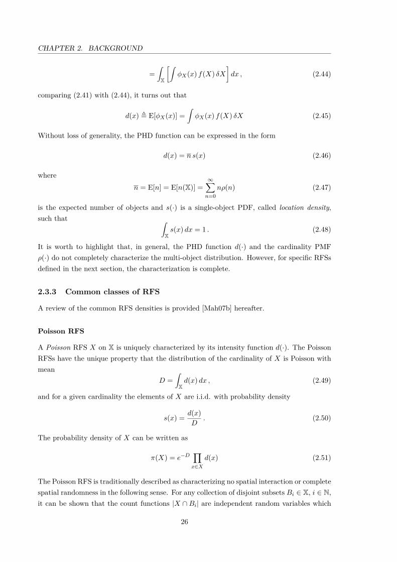
2.3.3 Common classes of RFS
A review of the common RFS densities is provided [Mah07b] hereafter.
Poisson RFS
A Poisson RFS X on X is uniquely characterized by its intensity function d(·). The PoissonRFSs have the unique property that the distribution of the cardinality of X is Poisson withmean
D =∫Xd(x) dx , (2.49)
and for a given cardinality the elements of X are i.i.d. with probability density
s(x) = d(x)D
. (2.50)
The probability density of X can be written as
π(X) = e−D∏x∈X
d(x) (2.51)
The Poisson RFS is traditionally described as characterizing no spatial interaction or completespatial randomness in the following sense. For any collection of disjoint subsets Bi ∈ X, i ∈ N,it can be shown that the count functions |X ∩Bi| are independent random variables which
26

2.3. RANDOM FINITE SET APPROACH
are Poisson distributed with mean
DBi =∫Bi
d(x) dx , (2.52)
and for a given number of points occurring in Bi the individual points are i.i.d. according to
d(x) 1Bi(x)NBi
. (2.53)
The procedure in Table 2.7 illustrates how to generate a sample from a Poisson RFS.
Table 2.7: Sampling a Poisson RFS
X = ∅Sample n ∼ Poisson[D]for i = 1, . . . , n do
Sample xi ∼ s(·)X = X ∪ x
end for
Independent identically distributed cluster RFS
An i.i.d. cluster RFS X on X is uniquely characterized by its cardinality distribution ρ(·)and matching intensity function d(·). The cardinality distribution must satisfy
D =∞∑n=0
nρ(n) =∫Xd(x) dx , (2.54)
but can otherwise be arbitrary, and for a given cardinality the elements of X are i.i.d. withprobability density
s(x) = d(x)D
(2.55)
The probability density of an i.i.d. cluster RFS can be written as
π(X) = |X|! ρ(|X|)∏x∈X
s(x) (2.56)
Note that an i.i.d. cluster RFS essentially captures the spatial randomness of the PoissonRFS without the restriction of a Poisson cardinality distribution. The procedure in Table 2.8illustrates how a sample from an i.i.d. RFS is generated.
Bernoulli RFS
A Bernoulli RFS X on X has probability q , 1− r of being empty, and probability r of beinga singleton whose only element is distributed according to a probability density p defined
27

CHAPTER 2. BACKGROUND
Table 2.8: Sampling an i.i.d. RFS
X = ∅Sample n ∼ ρ(·)for i = 1, . . . , n do
Sample xi ∼ s(·)X = X ∪ x
end for
on X. The cardinality distribution of a Bernoulli RFS is thus a Bernoulli distribution withparameter r. A Bernoulli RFS is completely described by the parameter pair (r, p(·)).
Multi-Bernoulli RFS
A multi-Bernoulli RFS X on X is a union of a fixed number of independent Bernoulli RFSsX(i) with existence probability r(i) ∈ (0, 1) and probability density p(i)(·) defined on X fori = 1, . . . , I, i.e.
X =I⋃i=1
X(i) . (2.57)
It follows that the mean cardinality of a multi-Bernoulli RFS is
D =I∑i=1
r(i) (2.58)
A multi-Bernoulli RFS is thus completely described by the corresponding multi-Bernoulliparameter set
(r(i), p(i)(·)
)Ii=1
. Its probability density is
π(X) =I∏j=1
(1− r(j)
) ∑1≤i1 6=···6=i|X|≤I
|X|∏j=1
r(ij) p(ij)(xj)1− r(ij) (2.59)
For convenience, probability densities of the form (2.59) are abbreviated by the form π(X) =(r(i), p(i)
)Ii=1
. A multi-Bernoulli RFS jointly characterizes unions of non-interacting pointswith less than unity probability of occurrence and arbitrary spatial distributions. The pro-cedure in Table 2.9 illustrates how a sample from a multi-Bernoulli RFS is generated.
2.3.4 Bayesian multi-object filtering
Let us now introduce the basic ingredients of the MOF problem [Mah07b, Mah04, Mah13,Mah14], i.e. the object RFS Xk ⊂ X at time k and the RFS Y i
k of measurements gatheredby node i ∈ N at time k. It is also convenient to define the overall measurement RFSs attime k,
Yk ,⋃i∈N
Y ik , (2.60)
28

2.3. RANDOM FINITE SET APPROACH
Table 2.9: Sampling a multi-Bernoulli RFS
X = ∅for i = 1, . . . , I do
Sample u ∼ Uniform[0,1]if u ≤ r(i) then
Sample x ∼ p(i)(·)X = X ∪ x
end ifend for
and up to time k,
Y1:k ,k⋃
κ=1Yκ . (2.61)
In the random set framework, the Bayesian approach to MOF consists, therefore, of recur-sively estimating the object set Xk conditioned to the observations Y1:k. The object set isassumed to evolve according to a multi-object dynamics
Xk = Φk−1(Xk−1) ∪Bk−1 (2.62)
where Bk−1 is the RFS of new-born objects at time k − 1 and
Φk−1(X) =⋃x∈X
φk−1(x) , (2.63)
φk−1(x) =
x′ , with survival probability PS,k−1
∅ , otherwise(2.64)
Notice that according to (2.62)-(2.64) each object in the set Xk is either a new-born objectfrom the set Bk−1 or an object survived from Xk−1, with probability PS,k−1, and whosestate vector x′ has evolved according to the single-object dynamics (2.2) with x = xk−1 andx′ = xk. In a similar way, observations are assumed to be generated, at each node i ∈ N ,according to the measurement model
Y ik = Ψi
k(Xk) ∪ Cik (2.65)
where Cik is the clutter RFS (i.e. the set of measurements not due to objects) at time k andnode i, and
Ψik(X) =
⋃x∈X
ψik(x) , (2.66)
ψik(x) =
yk , with detection probability PD,k
∅ , otherwise(2.67)
29

CHAPTER 2. BACKGROUND
Notice that according to (2.65)-(2.67) each measurement in the set Y ik is either a false one
from the clutter set Cik or is related to an object in Xk, with probability PD,k, according tothe single-sensor measurement equation (2.4). Hence it is clear how one of the major benefitsof the random set approach is to directly include in the MOF problem formulation (2.62)-(2.67) fundamental practical issues such as object birth and death, false alarms (clutter)and missed detections. Following a Bayesian approach, the aim is to propagate in time theposterior (filtered) multi-object densities πk(X) of the object set Xk given Y1:k, as well as theprior (predicted) ones πk|k−1(X) of Xk given Y1:k−1. Exploiting random set theory, it hasbeen found [Mah07b] that the multi-object densities follow recursions that are conceptuallyanalogous to the well-known ones of Bayesian nonlinear filtering, i.e.
πk|k−1(X) =∫ϕk|k−1(X|Z)πk−1(Z) δZ , (2.68)
πk(X) =gk(Yk|X)πk|k−1(X)∫gk(Yk|Z)πk|k−1(Z) δZ
, (2.69)
where ϕk|k−1( · | · ) is the multi-object transition density to time k, gk( · | · ) is the multi-objectlikelihood function at time k [Mah03,Mah07a,Mah07b].
Remark 6. Despite this conceptual resemblance, however, the multi-object Bayes recursions(2.68)-(2.69), unlike their single-object counterparts, are affected by combinatorial complexityand are, therefore, computationally infeasible except for very small-scale MOF problemsinvolving few objects and/or measurements.
For this reason, the computationally tractable PHD and Cardinalized PHD (CPHD) fil-tering approaches will be followed and briefly reviewed.
2.3.5 CPHD filtering
The CPHD filter [Mah07a, VVC07] propagates in time the cardinality PMFs ρk|k−1(n) andρk(n) as well as the PHD functions dk|k−1(x) and dk(x) of Xk given Y1:k−1 and, respectively,Y1:k assuming that the clutter RFS, the predicted and filtered RFSs are i.i.d. cluster processes(see (2.56)). The resulting CPHD recursions (prediction and correction) are as follows
Prediction
ρk|k−1(n) =n∑j=0
pb(n− j) ρS,k|k−1(j)
dk|k−1(x) = db,k(x) +∫ϕk|k−1(x|ζ) PS,k−1(ζ) dk−1(ζ) dζ
(2.70)
Correction
30

2.3. RANDOM FINITE SET APPROACH
ρk(n) =G0k
(dk|k−1(·) , Yk, n
)ρk|k−1(n)
∞∑η=0G0k
(dk|k−1(·) , Yk, η
)ρk|k−1(η)
dk(x) = GYk(x) dk|k−1(x)
(2.71)
where: pb,k(·) is the assumed birth cardinality PMF; ρS,k|k−1(·) is the cardinality PMF ofsurvived objects, given by
ρS,k|k−1(j) =∞∑t=j
t
j
P jS,k (1− PS,k)h−j ρk−1(t) ; (2.72)
db,k(·) is the assumed PHD function of new-born objects; ϕk|k−1(x|ξ) is the state transitionPDF (2.3) associated to the single object dynamics; the generalized likelihood functionsG0k(·, ·, ·) and GYk
(·) have cumbersome expressions which can be found in [VVC07].Enforcing Poisson cardinality distributions for the clutter and object sets, the update
of the cardinality PMF is no longer needed and the CPHD filter reduces to the PHD filter[Mah03,VM06]. The CPHD filter provides enhanced robustness with respect to misdetections,clutter as well as various uncertainties on the multi-object model (i.e. detection and survivalprobabilities, clutter and birth distributions) at the price of an increased computational load:a CPHD recursion has O(m3nmax) complexity compared to O(mnmax) of PHD, m being thenumber of measurements and nmax the maximum number of objects. There are essentiallytwo ways of implementing PHD/CPHD filters, namely the Particle Filter (PF) or SequentialMonte Carlo (SMC) [VSD05] and the Gaussian Mixture (GM) [VM06, VVC07] approaches,the latter being cheaper in terms of computation and memory requirements and, hence, byfar preferable for distributed implementation on a sensor network wherein nodes have limitedprocessing and communication capabilities.
2.3.6 Labeled RFSs
The aim of MOT is not only to recursively estimate the state of the objects and their timevarying number, but also to keep track of their trajectories. To this end, the notion of labelis introduced in the RFS approach [VV13, VVP14] so that each estimated object can beuniquely identified and its track reconstructed.
Let L : X×L → L be the projection L((x, `)) = `, where X ⊆ Rnx , L = αi : i ∈ Nand αi’s are distinct. To estimate the trajectories of the objects they need to be uniquelyidentified by a (unobserved) label drawn from a discrete countable space L = αi : i ∈ N,where the αi’s are distinct. To incorporate object identity, a label ` ∈ L is appended tothe state x of each object and the multi-object state is regarded as a finite set on X× L, i.e.x , (x, `) ∈ X×L. However, this idea alone is not enough since L is discrete and it is possible(with non-zero probability) that multiple objects have the same identity, i.e. be marked with
31

CHAPTER 2. BACKGROUND
the same label. This problem can be alleviated using a special case of RFS called labeledRFS [VV13,VVP14], which is, in essence, a marked RFS with distinct labels. Then, a finitesubset X of X×L has distinct labels if and only if X and its labels L(X) = L(x) : x ∈ Xhave the same cardinality, i.e. |X| = |L(X)|. The function ∆(X) , δ|X|(|L(X)|) is called thedistinct label indicator and assumes value 1 if and only if the condition |X| = |L(X)| holds.
Definition 2. A labeled RFS with state space X and (discrete) label space L is an RFS onX× L such that each realization X has distinct labels, i.e.
|X| = |L(X)| . (2.73)
The unlabeled version of a labeled RFS with density π is distributed according to themarginal density [VV13]
π(x1, . . . , xn) =∑
(`1,...,`n)∈Ln
π((x1, `1) , . . . , (xn, `n)) . (2.74)
The unlabeled version of a labeled RFS is its projection from X× L into X, and is obtainedby simply discarding the labels. The cardinality distribution of a labeled RFS is the same asits unlabeled version [VV13].
Hereinafter, symbols for labeled states and their distributions are bolded to distinguishthem from unlabeled ones, e.g. x, X, π, etc.
2.3.7 Common classes of labeled RFS
A review of the common labeled RFS densities is provided [VV13].
Labeled Poisson RFS
A labeled Poisson RFS X with state space X and label space L = αi : i ∈ N, is a PoissonRFS X on X with intensity d(·), tagged with labels from L. A sample from such labeledPoisson RFS can be generated by the procedure reported in Table 2.10.
Table 2.10: Sampling a labeled Poisson RFS
X = ∅Sample n ∼ Poisson[D]for i = 1, . . . , n do
Sample x ∼ d(·) /DX = X ∪ (x, αi)
end for
The probability density of an LMB RFS is given by
π(X) = δL(|X|)(L(X)) Poisson[D](|X|)∏
x∈X
d(x)D
, (2.75)
32

2.3. RANDOM FINITE SET APPROACH
where L(n) = αi ∈ Lni=1; δL(n)(`1, . . . , `n) serves to check whether or not labels are dis-tinct.
Remark 7. By a tracking point of view, each label of a labeled Poisson RFS X cannotdirectly refer to an object since all the corresponding states are sampled from the sameintensity d(x), i.e. there is not a 1-to-1 mapping between labels and location PDFs. Thus, itis not clear how to properly use such a labeled distribution in a MOT problem.
Labeled independent identically distributed cluster RFS
In the same fashion of the unlabeled RFSs, the labeled Poisson RFS can be generalized tothe labeled i.i.d. cluster RFS by removing the Poisson assumption on the cardinality andspecifying an arbitrary cardinality distribution. A sample from such a labeled i.i.d. RFS canbe generated by the procedure reported in Table 2.11.
Table 2.11: Sampling a labeled i.i.d. cluster RFS
X = ∅Sample n ∼ ρ(·)for i = 1, . . . , n do
Sample x ∼ d(·) /DX = X ∪ (x, αi)
end for
The probability density of an LMB RFS is given by
π(X) = δL(|X|)(L(X)) ρ(|X|)∏
x∈X
d(x)D
, (2.76)
The same consideration drawn for the labeled Poisson RFS is inherited by the i.i.d. clusterRFS.
Generalized Labeled Multi-Bernoulli RFS
A Generalized Labeled Multi-Bernoulli (GLMB) RFS [VV13] is a labeled RFS with statespace X and (discrete) label space L distributed according to
π(X) = ∆(X)∑c∈C
w(c)(L(X))[p(c)
]X(2.77)
where: C is a discrete index set; w(c)(L) and p(c) satisfy the normalization constraints:
∑L⊆L
∑c∈C
w(c)(L) = 1 , (2.78)∫p(c)(x, `) dx = 1 . (2.79)
33

CHAPTER 2. BACKGROUND
A GLMB can be interpreted as a mixture of |C| multi-object exponentials
w(c)(L(X))[p(c)
]X. (2.80)
Each term in the mixture (2.77) consists of the product of two factors:
1. a weight w(c)(L(X)) that only depends on the labels L(X) of the multi-object state X;
2. a multi-object exponential[p(c)
]Xthat depends on the entire multi-object state.
The cardinality distribution of a GLMB is given by
ρ(n) =∑
L∈Fn(L)
∑c∈C
w(c)(L) , (2.81)
from which, in fact, summing over all possible n implies (2.78). The PHD of the unlabeledversion of a GLMB is given by
d(x) =∑c∈C
∑`∈L
p(c)(x, `)∑L⊆L
1L(`)w(c)(L) . (2.82)
Remark 8. The GLMB RFS distribution has the appealing feature of having a 1-to-1 map-ping between labels and location PDFs provided by the single-object densities p(c)(x, `), foreach term of the multi-object exponential mixture indexed with c. However, in the contextof MOT, it is not clear how to exploit (in particular how to implement) such a distribu-tion [VV13,VVP14].
δ-Generalized Labeled Multi-Bernoulli RFS
A δ-Generalized Labeled Multi-Bernoulli (δ-GLMB) RFS with state space X and (discrete)label space L is a special case of a GLMB with
C = F(L)× Ξ , (2.83)
w(c)(L) = w(I,ξ)(L) = w(I,ξ)δI(L) , (2.84)
p(c)(·) = p(I,ξ)(·) = p(ξ)(·) , (2.85)
i.e. is distributed according to
π(X) = ∆(X)∑
(I,ξ)∈F(L)×Ξw(I,ξ)δI(L(X))
[p(ξ)
]X(2.86)
= ∆(X)∑
I∈F(L)δI(L(X))
∑ξ∈Ξ
w(I,ξ)[p(ξ)
]X, (2.87)
where Ξ is a discrete space. In MOT a δ-GLMB can be used (and implemented) to representthe multi-object densities over time. In particular:
34
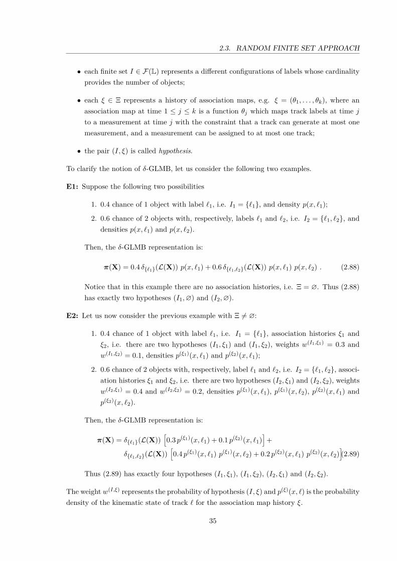
2.3. RANDOM FINITE SET APPROACH
• each finite set I ∈ F(L) represents a different configurations of labels whose cardinalityprovides the number of objects;
• each ξ ∈ Ξ represents a history of association maps, e.g. ξ = (θ1, . . . , θk), where anassociation map at time 1 ≤ j ≤ k is a function θj which maps track labels at time jto a measurement at time j with the constraint that a track can generate at most onemeasurement, and a measurement can be assigned to at most one track;
• the pair (I, ξ) is called hypothesis.
To clarify the notion of δ-GLMB, let us consider the following two examples.
E1: Suppose the following two possibilities
1. 0.4 chance of 1 object with label `1, i.e. I1 = `1, and density p(x, `1);
2. 0.6 chance of 2 objects with, respectively, labels `1 and `2, i.e. I2 = `1, `2, anddensities p(x, `1) and p(x, `2).
Then, the δ-GLMB representation is:
π(X) = 0.4 δ`1(L(X)) p(x, `1) + 0.6 δ`1,`2(L(X)) p(x, `1) p(x, `2) . (2.88)
Notice that in this example there are no association histories, i.e. Ξ = ∅. Thus (2.88)has exactly two hypotheses (I1,∅) and (I2,∅).
E2: Let us now consider the previous example with Ξ 6= ∅:
1. 0.4 chance of 1 object with label `1, i.e. I1 = `1, association histories ξ1 andξ2, i.e. there are two hypotheses (I1, ξ1) and (I1, ξ2), weights w(I1,ξ1) = 0.3 andw(I1,ξ2) = 0.1, densities p(ξ1)(x, `1) and p(ξ2)(x, `1);
2. 0.6 chance of 2 objects with, respectively, label `1 and `2, i.e. I2 = `1, `2, associ-ation histories ξ1 and ξ2, i.e. there are two hypotheses (I2, ξ1) and (I2, ξ2), weightsw(I2,ξ1) = 0.4 and w(I2,ξ2) = 0.2, densities p(ξ1)(x, `1), p(ξ1)(x, `2), p(ξ2)(x, `1) andp(ξ2)(x, `2).
Then, the δ-GLMB representation is:
π(X) = δ`1(L(X))[0.3 p(ξ1)(x, `1) + 0.1 p(ξ2)(x, `1)
]+
δ`1,`2(L(X))[0.4 p(ξ1)(x, `1) p(ξ1)(x, `2) + 0.2 p(ξ2)(x, `1) p(ξ2)(x, `2)
].(2.89)
Thus (2.89) has exactly four hypotheses (I1, ξ1), (I1, ξ2), (I2, ξ1) and (I2, ξ2).
The weight w(I,ξ) represents the probability of hypothesis (I, ξ) and p(ξ)(x, `) is the probabilitydensity of the kinematic state of track ` for the association map history ξ.
35

CHAPTER 2. BACKGROUND
Labeled Multi-Bernoulli RFS
A labeled multi-Bernoulli (LMB) RFS X with state space X, label space L and (finite)parameter set (r(`), p(`)) : ` ∈ L, is a multi-Bernoulli RFS on X augmented with labelscorresponding to the successful (non-empty) Bernoulli components. In particular, r(`) is theexistence probability and p(`) is the PDF on the state space X of the Bernoulli component(r(`), p(`)) with unique label ` ∈ L. The procedure in Table 2.12 illustrates how a samplefrom a labeled multi-Bernoulli RFS is generated.
Table 2.12: Sampling a labeled multi-Bernoulli RFS
X = ∅for ` ∈ L do
Sample u ∼ Uniform[0,1]if u ≤ r(`) then
Sample x ∼ p(`)(·)X = X ∪ (x, `)
end ifend for
The probability density of an LMB RFS is given by
π(X) = ∆(X)w(L(X)) pX (2.90)
where
w(L) =∏`∈L
1L(`) r(`) ∏`∈L\L
(1− r(`)
), (2.91)
p(`)(x) , p(x, `) . (2.92)
For convenience, the shorthand notation π =(r(`), p(`)
)`∈L
will be adopted for the densityof an LMB RFS. The LMB is also a special case of the GLMB [VV13, VVP14, RVVD14]having C with a single element (thus the superscript is simply avoided) and
p(c)(x, `) = p(x, `) = p(`)(x) , (2.93)
w(c)(L) = w(L) . (2.94)
2.3.8 Bayesian multi-object tracking
The labeled RFS paradigm [VV13, VVP14], along with the mathematical tools provided byFISST [Mah07b], allows to formalize in a rigorous and elegant way the multi-object Bayesianrecursion for MOT.
For MOT, the object label is an ordered pair of integers ` = (k, i), where k is the time
36

2.3. RANDOM FINITE SET APPROACH
of birth and i ∈ N is a unique index to distinguish objects born at the same time. Thelabel space for objects born at time k is Lk = k × N. An object born at time k has statex ∈ X × Lk. Hence, the label space for objects at time k (including those born prior to k),denoted as L0:k, is constructed recursively by L0:k = L0:k−1 ∪ Lk (note that L0:k−1 and Lkare disjoint). A multi-object state X at time k is a finite subset of X× L0:k.
Suppose that, at time k, there are Nk objects with states xk,1, . . . ,xk,Nk, each taking
values in the (labeled) state space X×L0:k, and Mk measurements yk,1, . . . , yk,Mkeach taking
values in an observation space Y. The multi-object state and multi-object observation, at timek, [Mah03,Mah07b] are, respectively, the finite sets
Xk = xk,1, . . . ,xk,Nk , (2.95)
Yk = yk,1, . . . , yk,Mk . (2.96)
Let πk(·) denote the multi-object filtering density at time k, and πk|k−1(·) the multi-objectprediction density to time k (formally πk(·) and πk|k−1(·) should be written respectivelyas πk(·|Y0, . . . , Yk−1, Yk), and πk|k−1(·|Y0, . . . , Yk−1), but for simplicity the dependence onpast measurements is omitted). Then, the multi-object Bayes recursion propagates πk intime [Mah03,Mah07b] according to the following update and prediction
πk|k−1(X) =∫ϕk|k−1(X|Z)πk−1(Z) δZ , (2.97)
πk(X) =gk(Yk|X)πk|k−1(X)∫gk(Yk|Z)πk|k−1(Z) δZ
, (2.98)
where ϕk|k−1( · | · ) is the labeled multi-object transition density to time k, gk( · | · ) is the multi-object likelihood function at time k, and the integral is a set integral defined, for any functionf : F(X× L)→ R, by
∫f(X) δX =
∞∑n=0
1n!
∑(`1,...,`n)∈L
∫Xnf((x1, `1) , . . . , (xn, `n)) dx1 · · · dxn . (2.99)
The multi-object posterior density captures all information on the number of objects, andtheir states [Mah07b]. The multi-object likelihood function encapsulates the underlying mod-els for detections and false alarms while the multi-object transition density embeds the un-derlying models of motion, birth and death [Mah07b].
Remark 9. Eqs. (2.97)-(2.98) represent the multi-object counterpart of (2.7)-(2.8).
Let us now consider a multi-sensor centralized setting in which a sensor network (N ,A)conveys all the measurement to a central fusion node. Assuming that the measurementstaken by the sensors are independent, the multi-object Bayesian filtering recursion can be
37

CHAPTER 2. BACKGROUND
naturally extended as follows:
πk|k−1(X) =∫ϕk|k−1(X|Z)πk−1(Z) δZ , (2.100)
πk(X) =
∏i∈N
gik
(Y ik |X
)πk|k−1(X)∫ ∏
i∈Ngik
(Y ik |Z
)πk|k−1(Z) δZ
, (2.101)
Remark 10. Eqs. (2.100)-(2.101) represents the multi-object counterpart of (2.9)-(2.10)which has been made possible thanks to the concept of RFS densities.
In the work [VV13], the full labeled multi-object Bayesian recursion is derived for thegeneral class of GLMB densities, while in [VVP14] the analytical implementation of themulti-object Bayesian recursion for the δ-GLMB density is provided. Moreover, in the work[RVVD14], a multi-object Bayesian recursion for the LMB density, which turns out not to bein a closed form, is discussed and presented.
For convenience, hereinafter, explicit reference to the time index k for label sets will beomitted by denoting L− , L0:k−1, B , Lk, L , L− ∪ B.
2.4 Distributed information fusion
The third and fourth core concepts of this dissertation are the Kullback-Leibler Average(KLA) and consensus, which are two mathematical tools for distributing information oversensor networks.
To combine limited information from individual nodes, a suitable information fusion pro-cedure is required to reconstruct, from the information of the various local nodes, the state ofthe objects present in the surrounding environment. The scalability requirement, the lack of afusion center and knowledge on the network topology (see section 2.1) dictate the adoption ofa consensus approach to achieve a collective fusion over the network by iterating local fusionsteps among neighboring nodes [OSFM07,XBL05,CA09,BC14]. In addition, due to the dataincest problem in the presence of network loops that causes double counting of information,robust (but suboptimal) fusion rules, such as the Chernoff fusion rule [CT12,CCM10] (thatincludes Covariance Intersection [JU97,Jul08] and its generalization [Mah00]) are required.
In this chapter, the KLA and consensus will be separately dealt with, respectively, as arobust suboptimal fusion rule and as a technique to spread information, in a scalable way,throughout sensor networks.
38

2.4. DISTRIBUTED INFORMATION FUSION
2.4.1 Notation
Given PDFs p, q and a scalar α > 0, the information fusion ⊕ and weighting operators [BCF+13a,BC14,BCF14a] are defined as follows
(p⊕ q) (x) , p(x) q(x)〈p, q〉
(2.102)
(α p) (x) , [p(x)]α
〈pα, 1〉 . (2.103)
It can be checked that the fusion and weighting operators satisfy the following properties:
p.a (p⊕ q)⊕ h = p⊕ (q ⊕ h) = p⊕ q ⊕ h
p.b p⊕ q = q ⊕ p
p.c (αβ) p = α (β p)
p.d 1 p = p
p.e α (p⊕ q) = (α p)⊕ (α q)
p.f (α+ β) p = (α p)⊕ (β q)
for any PDFs p and q, positive scalars α and β.
2.4.2 Kullback-Leibler average of PDFs
A key ingredient for networked estimation is the capability to fuse in a consistent way PDFsof the quantity to be estimated provided by different nodes. In this respect, a sensibleinformation-theoretic definition of fusion among PDFs is the Kullback-Leibler Average (KLA)[BCMP11,BC14] relying on the Kullback-Leibler Divergence (KLD). Given PDFs
pi(·)
i∈N
and relative weights ωi > 0 such that∑i∈N ω
i = 1, their weighted KLA p(·) is defined as
p(·) = arg infp(·)
∑i∈N
ωiDKL
(p ‖ pi
)(2.104)
whereDKL
(p ‖ pi
)=∫p(x) log
(p(x)pi(x)
)dx (2.105)
denotes the KLD between the PDFs p (·) and pi(·). In [BC14] it is shown that the weightedKLA in (2.104) coincides with the normalized weighted geometric mean (NWGM) of thePDFs, i.e.
p(x) =
∏i∈N
[pi(x)
]ωi
∫ ∏i∈N
[pi(x)
]ωi
dx
,⊕i∈N
(ωi pi(x)
)(2.106)
39

CHAPTER 2. BACKGROUND
where the latter equality follows from the properties of the operators and ⊕. Note that inthe unweighted KLA ωi = 1/ |N |, i.e.
p (x) =⊕i∈N
( 1|N | pi
)(x) . (2.107)
If all PDFs are Gaussian, i.e. pi(·) = N(· ; mi, P i
), p(·) in (2.106) turns out to be Gaussian
[BC14], i.e. p(·) = N(· ; m,P
). In particular, defining the information (inverse covariance)
matrixΩ , P−1 (2.108)
and information vectorq , P−1m (2.109)
associated to the Gaussian mean m and covariance P , one has
Ω =∑i∈N
ωiΩi , (2.110)
q =∑i∈N
ωiqi . (2.111)
which corresponds to the well known Covariance Intersection (CI) fusion rule [JU97]. Hencethe KLA of Gaussian PDFs is a Gaussian PDF whose information pair (Ω, q) is obtainedby the weighted arithmetic mean of the information pairs (Ωi, qi) of the averaged GaussianPDFs.
2.4.3 Consensus algorithms
In recent years, consensus algorithms have emerged as a powerful tool for distributed com-putation over networks [OSFM07,XBL05] and have been widely used in distributed parame-ter/state estimation algorithms [OS07,KT08,CS10,CCSZ08,CA09,SSS09,BCMP11,FFTS10,LJ12, HSH+12, BCF+13a, BC14, OHD14, BCF14a, BCF+14b, FBC+12, BCF+13b, BCF+13c,BCF+13d,BCF+14c]. In its basic form, a consensus algorithm can be seen as a technique fordistributed averaging over a network; each agent aims to compute the collective average ofa given quantity by iterative regional averages, where the terms “collective” and “regional”mean “over all network nodes” and, respectively, “over neighboring nodes only”. Consensuscan be exploited to develop scalable and reliable distributed fusion techniques.
To this end, let us briefly introduce a prototypal average consensus problem. Let nodei ∈ N be provided with an estimate θi of a given quantity of interest θ. The objective is todevelop an algorithm that computes in a distributed way, in each node, the average
θ = 1|N |
∑i∈N
θi . (2.112)
40

2.4. DISTRIBUTED INFORMATION FUSION
To this end, let θi0 = θi, then a simple consensus algorithm takes the following iterative form:
θil+1 =∑j∈N i
ωi,j θjl , ∀i ∈ N (2.113)
where the consensus weights must satisfy the conditions
∑j∈N i
ωi,j = 1 , ∀i ∈ N (2.114)
ωi,j ≥ 0 , ∀i, j ∈ N . (2.115)
Notice from (2.113)-(2.115) that at a given consensus step the estimate in any node is com-puted as a convex combination of the estimates of the neighbors at the previous consensusstep. In other words, the iteration (2.113) is simply a regional average computed in nodei, the objective of consensus being convergence of such regional averages to the collectiveaverage (2.112). Important convergence properties, depending on the consensus weights, canbe found in [OSFM07,XBL05]. For instance, let us denote by Π the consensus matrix whosegeneric (i, j)-element coincides with the consensus weight ωi,j (if j /∈ N i then ωi,j is takenas 0). Then, if the consensus matrix Π is primitive and doubly stochastic1, the consensusalgorithm (2.119) asymptotically yields the average (2.112) in that
liml→∞
θi = θ , ∀i ∈ N . (2.116)
A necessary condition for the matrix Π to be primitive is that the graph G associated withthe sensor network be strongly connected [CA09]. Moreover, in the case of an undirectedgraph G, a possible choice ensuring convergence to the collective average is given by theso-called Metropolis weights [XBL05,CA09].
ωi,j = 11 + max|N i| , |N j |
, i ∈ N , j ∈ N i , i 6= j (2.117)
ωi,i = 1−∑
j∈N i, j 6=iωi,j . (2.118)
2.4.4 Consensus on posteriors
The idea is to exploit consensus to reach a collective agreement (over the entire network),by having each node iteratively updating and passing its local information to neighbouringnodes. Such repeated local operations provide a mechanism for propagating informationthroughout the whole network. The idea is to perform, at each time instant and in eachnode of the network i ∈ N , a local correction step to find the local posterior PDF followedby consensus on such posterior PDFs to determine the collective unweighted KLA of theposterior densities pik.
1A non-negative square matrix Π is doubly stochastic if all its rows and columns sum up to 1. Further, itis primitive if there exists an integer m such that all the elements of Πm are strictly positive.
41

CHAPTER 2. BACKGROUND
Suppose that at time k, each agent i starts with the posterior pik as the initial iterate pik,0,and computes the l-th consensus iterate by
pik,l =⊕j∈N i
(ωi,j pjk,l−1
)(2.119)
where ωi,j ≥ 0, satisfying∑j∈N i ωi,j = 1, are the consensus weights relating agent i to nodes
j ∈ N i. Then, using the properties of the operators ⊕ and , it can be shown that [BC14]
pik,l =⊕j∈N
(ωi,jl p
jk
)(2.120)
where ωi,jl is the (i, j)-th entry of Πn, with Π the (square) consensus matrix with (i, j)-thentry ωi,j1N i(j) (it is understood that pjk is omitted from the fusion whenever ωi,jl = 0).More importantly, it was shown in [OSFM07, XBL05] that if the consensus matrix Π isprimitive, (i.e. non-negative, and there exists an integer m such that Πm is positive) anddoubly stochastic (all rows and columns sum to 1), then for any i, j ∈ N , one has
liml→∞
ωi,jl = 1|N |
. (2.121)
In other words, at time k, if the consensus matrix is primitive then the consensus iterate ofeach node in the network “tends” to the collective unweighted KLA (2.107) of the posteriordensities [CA09,BC14].
The Consensus on Posteriors (CP) approach to Distributed SOF (DSOF) is summarizedby the algorithm of Table 2.13 to be carried out at each sampling interval k in each nodei ∈ N . In the linear Gaussian case, the CP algorithm involves a Kalman filter for localprediction and correction steps and CI for the consensus steps. In this case, it has beenbeen proved [BCMP11, BC14] that, under suitable assumptions, the CP algorithm guaran-tees mean-squared bounded estimation error in all network nodes for any number L ≥ 1 ofconsensus iterations. In the nonlinear and/or non Gaussian case, the PDFs in the varioussteps can be approximated as Gaussian and the corresponding means-covariances updatedvia, e.g., EKF [MSS62] or UKF [JU04].
Remark 11. Whenever the number of consensus steps L tends to infinity, consensus onposteriors is unable to recover the solution of the Bayesian filtering problem. In fact, in the CPapproach, the novel information undergoing consensus combined with the prior information,is unavoidably underweighted.
42

2.4. DISTRIBUTED INFORMATION FUSION
Table 2.13: Consensus on Posteriors (CP)
procedure CP(Node i, Time k)Predictionpik|k−1(xk) =
∫ϕk|k−1(xk|xk−1) pik−1(xk−1) dxk−1
Local Correction
pik(xk|yik
)=
(gik(yik|·
)⊕ pik|k−1(·)
)(x) , i ∈ S
pik|k−1(xk) , i ∈ C
Consensuspik,0(xk) = pik
(xk|yik
)for l = 1, . . . , L do
pik,l(xk) =⊕j∈N i
(ωi,j pjk,l−1(x)
)end forpik(xk) = pik,L(xk)
end procedure
43


3 Distributedsingle-object filtering
Contents3.1 Consensus-based distributed filtering 45
3.1.1 Parallel consensus on likelihoods and priors 453.1.2 Approximate CLCP 483.1.3 A tracking case-study 50
3.2 Consensus-based distributed multiple-model filtering 513.2.1 Notation 523.2.2 Bayesian multiple-model filtering 523.2.3 Networked multiple model estimation via consensus 543.2.4 Distributed multiple-model algorithms 553.2.5 Connection with existing approach 563.2.6 A tracking case-study 58
This chapter presents two applications of distributed information fusion for single-objectfiltering [BCF14a,FBC+12,BCF+14b]. The first application presents an improvement of theCP approach, described in subsection 2.4.4, and is applied to track a single non-maneuveringobject. The second application takes into account the possibility of the object of being highlymaneuvering. Thus, a multiple-model filtering approach is used to devise a consensus-basedalgorithm capable of tracking a single highly-maneuvering object. The effectiveness of theproposed algorithms is demonstrated via simulation experiments on realistic scenarios.
3.1 Consensus-based distributed filtering
The approach proposed in this section is based on the idea of carrying out, in parallel, aseparate consensus for the novel information (likelihoods) and one for the prior information(priors). This parallel procedure is conceived as an improvement of the CP approach toavoid underweighting the novel information during the fusion steps. The outcomes of the twoconsensuses are then combined to provide the fused posterior density.
3.1.1 Parallel consensus on likelihoods and priors
The proposed parallel Consensus on Likelihoods and Priors (CLCP) approach to DSOF issummarized by the algorithm of Table 3.1 to be carried out at each sampling interval k in
45

CHAPTER 3. DISTRIBUTED SINGLE-OBJECT FILTERING
each node i ∈ N . Notice that in the correction step, a suitable positive weight ρik ≥ 1 is
Table 3.1: Consensus on Likelihoods and Priors (CLCP) pseudo-code
procedure CLCP(Node i, Time k)Predictionpik|k−1(x) =
∫ϕk|k−1(x|ζ) pik−1(x) dζ
Consensus
gik,0(x) =
gik(yik|x
), i ∈ S
1 , i ∈ Cpik|k−1,0(x) = pik|k−1(x)
for l = 1, . . . , L dogik,l(x) =
⊕j∈N i
(ωi,j gjk,l−1(x)
)pik|k−1,l(x) =
⊕j∈N i
(ωi,j pjk|k−1,l−1(x)
)end for
Correctionpik(x) = pik|k−1,L(x)⊕
(ρik gik,L (x)
)end procedure
applied to the outcome of the consensus on likelihoods, in order to possibly counteract theunderweighting of novel information. To elaborate more on this issue, observe that each localposterior PDF pik(x) resulting from application of the CLCP algorithm turns out to be equalto
pik(x) =
⊕j∈N
(ωi,jL p
jk|k−1(x)
)⊕⊕j∈S
(ρikω
i,jL g
ik
(yik|x
)) . (3.1)
As it can be seen, pik(x) is composed of two parts: i) a weighted geometric mean of the priorspjk|k−1(x); ii) a weighted combination of the likelihoods gik
(yik|x
). The fact that in the first part
the weights ωi,jL sum up to one ensures that no double counting of the common informationcontained in the priors can occur [Jul08,BJA12]. As for the second part, care must be takenin the choice of the scalar weights ρik. For instance, in order to avoid overweighting someof the likelihoods, it is important that, for any pair i, j, one has ρikω
i,jL ≤ 1. In this way,
each component of independent information is replaced with a conservative approximation,thus ensuring the conservativeness of the overall fusion rule [BJA12]. On the other hand, theproduct ρikω
i,jL should not be too small in order to avoid excessive underweighting. Based
on these considerations and recalling the consensus property (2.121), different strategies forchoosing ρik can be devised.
46

3.1. CONSENSUS-BASED DISTRIBUTED FILTERING
A reasonable choice would amount to letting
ρik = minj∈S
(1ωi,jL
)(3.2)
whenever at least one of the weights ωi,jL is different from zero. Such a choice would assign toρik the closest value to the true number of agents |N | of the network. This strategy is easilyapplicable when L = 1 but, unfortunately, for L > 1 requires that each node of the networkcan compute ΠL. In most settings, this is not possible and alternative solutions must beadopted.
For example, when L 1 and the matrix Π is primitive and doubly stochastic, one hasthat ωi,jL ≈ 1/|N | for any i, j. Then, in this case, one can let
ρik = |N | . (3.3)
Such a choice has the appealing feature of giving rise to a distributed algorithm convergingto the centralized one as L tends to infinity. However, when only a moderate number ofconsensus steps is performed, it leads to an overweighting of some likelihood components.Furthermore, the number of nodes |N | might be unknown, in particular for a time-varyingnetwork. Notice that when such a choice is adopted, due to the properties of the fusion ⊕ andweighting operators, the CLCP algorithm can be shown to be mathematically equivalent(in the sense that they would generate the same pik(x)) to the optimal distributed protocolof [OC10].
An alternative solution is to exploit consensus so as to compute, in a distributed way, anormalization factor to improve the filter performance while preserving consistency of eachlocal filter. For example, an estimate of the fraction |S|/|N | of sensor nodes in the networkcan be computed via the consensus algorithm
bik,l =∑j∈N i
ωi,j bjk,l−1, l = 1, . . . , L (3.4)
with the initialization bik,0 = 1 if i ∈ S, and bik,0 = 0 otherwise. Then, the choice
ρik =
1 , if bik,L = 0
1bik,L
, otherwise(3.5)
has the desirable property of ensuring that ρikωi,jL ≤ 1 for any i, j. Another positive feature
of (3.5) is that no a priori knowledge of the network is required.
47

CHAPTER 3. DISTRIBUTED SINGLE-OBJECT FILTERING
3.1.2 Approximate CLCP
It must be pointed out that unfortunately the CLCP recursion of Table 3.1 does not admit anexact analytical solution except for the linear Gaussian case. Henceforth it will be assumedthat the noises are Gaussian, i.e. wk ∼ N (0, Qk) and vik ∼ N
(0, Rik
), but that the system, i.e.
fk(·) and/or hik(·), might be nonlinear. The main issue is how to deal with nonlinear sensorsin the consensus on likelihoods as for the other tasks (i.e. consensus on priors, correction,prediction) it is well known how to handle nonlinearities exploiting, e.g., EKF [MSS62] orUKF [JU04] or particle filters [RAG04]. Under the Gaussian assumption, the local likelihoodstake the form
gik(x) = gik
(yik|x
)= N
(yik − hik(x); 0, Rik
)(3.6)
Whenever sensor i is linear, i.e. hik (x) = Cikx,
gik(x) ∝ e−12 (x>δΩi
kx−2x>δqik) (3.7)
whereδΩi
k ,(Cik)> (
Rik)−1
Cik ,
δqik ,(Cik)> (
Rik)−1
yik ,(3.8)
Then it is clear that multiplying, or exponentiating by suitable weights, the likelihoods gik(·) isequivalent to adding, or multiplying by such weights, the corresponding δΩi
k and δqik definedin (3.8). Then, in the case of linear Gaussian sensors, the consensus on likelihoods reducesto a consensus on the information pairs defined in (3.8). For nonlinear sensors, a sensibleapproach seems therefore to approximate the nonlinear measurement function hik(·) by alinear affine one, i.e.
hik (x) ∼= Cik
(x− xik|k−1
)+ hi
(xk|k−1
)(3.9)
and then replace the measurement equation (2.4) with yik = Cikxk + vik for a suitably definedpseudo-measurement
yik = yik − yik|k−1 + Cikxik|k−1 (3.10)
The sensor linearization (3.9) can be carried out for example by following the EKF paradigm.As an alternative, exploiting the unscented transform and the unscented information filter[Lee08], from xik|k−1 and the relative covariance P ik|k−1, one can get the σ-points xi,jk|k−1 andrelative weights ωj for j = 0, 1, . . . , 2n (n = dim(x)), and thus compute
yik|k−1 =2n∑j=0
ωj yi,jk|k−1, y
i,jk|k−1 = hik
(xi,jk|k−1
)(3.11)
P yx,ik|k−1 =2n∑j=0
ωj(yik|k−1 − y
i,jk|k−1
) (xik|k−1 − x
i,jk|k−1
)>(3.12)
Cik = P yx,ik|k−1
(P ik|k−1
)−1(3.13)
48

3.1. CONSENSUS-BASED DISTRIBUTED FILTERING
Summarizing the above derivations, the proposed consensus-based distributed nonlinear filteris detailed in Table 3.2.
The reason for performing in parallel consensus on priors and likelihoods is the counter-action of underweighting of the novel information contained in the likelihoods by using theweighting factor ρik. Clearly, such a choice requires transmitting, at each consensus step,approximately twice the number of floating-point data with respect to other algorithms likeCP. Notice that, depending on the packet size, this need not necessarily increase the packetrate.
Table 3.2: Analytical implementation of Consensus on Likelihoods and Priors (CLCP)
procedure CLCP(Node i, Time t)Consensus
If i ∈ S:
δΩik,0 =
(Cik)> (
Rik)−1
Cik
δqik,0 =(Cik)> (
Rik)−1
yik
If i ∈ C:
δΩik,0 = 0
δqik,0 = 0
Ωik|k−1,0 =
(P ik|k−1
)−1
qik|k−1,0 =(P ik|k−1
)−1xik|k−1
for l = 1, . . . , L doLikelihoodδΩi
k,l =∑j∈N i
ωi,jδΩjk,l−1
δqik,l =∑j∈N i
ωi,jδqjk,l−1
PriorΩik|k−1,l =
∑j∈N i
ωi,jΩjk|k−1,l−1
qik|k−1,l =∑j∈N i
ωi,jqjk|k−1,l−1
end for
CorrectionΩik = Ωi
k|k−1,L + ρik δΩik,L
qik = qik|k−1,L + ρik δqik,L
PredictionP ik =
(Ωik
)−1, xik =(Ωik
)−1qik
from xik, Pik compute xik+1|k, P
ik+1|k via UKF
end procedure
49

CHAPTER 3. DISTRIBUTED SINGLE-OBJECT FILTERING
3.1.3 A tracking case-study
To evaluate performance of the proposed approach, the networked object tracking scenario offig. 3.1 has been simulated. The network consists of 50 COM nodes and 10 SEN measuring the
[m] ×1040 1 2 3 4 5
[m]
×104
0
0.5
1
1.5
2
2.5
3
3.5
4
4.5
5
LinkSurveillance areaCOM nodeSEN nodeObject trajectory
Figure 3.1: Network and object trajectory.
Time Of Arrival (TOA), i.e. the object-to-sensor distance. A linear white-noise accelerationmodel [BSLK01, p. 270], with 4-dimensional state consisting of positions and velocitiesalong the coordinate axes, is assumed for the object motion; with this choice of the state,sensors are clearly nonlinear. Standard deviation of the measurement noise has been set to100 [m], the sampling interval to 5 [s], the duration of the simulation to 1500 [s], i.e. 300samples. In the above scenario, 1000 Monte Carlo trials with independent measurementnoise realizations have been performed. The Position Root Mean Square Error (PRMSE)averaged over time, Monte Carlo trials and nodes is reported in Table 3.3 for different valuesof L (number of consensus steps) and different consensus-based distributed nonlinear filters.In all simulations, Metropolis weights [CA09, XBL05] have been adopted for consensus. Foreach filter and each L two values are reported: the top one refers to the PRMSE computedover whole the simulation horizon, whereas the bottom one refers to the PRMSE computedafter the transient period. Three approaches are compared in the UKF variants: the CLCP,CP (Consensus on Posteriors) [BCMP11,BC14] and CL (Consensus on Likelihoods) whereinconsensus is carried out on the novel information only1. For the CLCP, three different
1In order to have a fair comparison, the CL algorithm is implemented as in Table 3.2 with the differencethat no consensus on the priors is performed.
50

3.2. CONSENSUS-BASED DISTRIBUTED MULTIPLE-MODEL FILTERING
choices for the weights ρik are considered. From Table 3.3, it can be seen that the weightchoice ρik = |N | provides the best performance only when L is sufficiently large, while forfew consensus steps the other choices are preferable. It is worth pointing out that the CLapproach, which becomes optimal as L → ∞, guarantees a bounded estimation error onlywhen the number L of consensus steps is sufficiently high (in Table 3.3 “−” indicates adivergent PRMSE).
Table 3.3: Performance comparison
CP CL CLCPChoice of ρik |N | (3.5) |N | minj∈S(1/ωi,jL )
1733 − 1909 − 1645L = 1
513 − 407 − 3321299 − 1182 1621 821
L = 2423 − 257 545 2261041 − 491 736 480
L = 3389 − 231 129 198936 4269 391 455 355
L = 4370 3238 219 118 182868 977 341 283 299
L = 5358 134 210 111 170
681 222 230 138 173L = 15
318 94 182 85 122
3.2 Consensus-based distributed multiple-model filtering
The section addresses distributed state estimation of jump Markovian systems and its appli-cation to tracking of a maneuvering object by means of a network of heterogeneous sen-sors and communication nodes. It is well known that a single-model Kalman-like filteris ineffective for tracking a highly maneuvering object and that Multiple Model (MM) fil-ters [AF70, BBS88, BSLK01, LJ05] are by far superior for this purpose. The contributionsprovide novel consensus MM filters to be used for tracking maneuvering objects with sensornetworks. Two novel consensus-based MM filters are presented. Simulation experiments ina tracking case-study, involving a strongly maneuvering object and a sensor network charac-terized by weak connectivity, demonstrate the superiority of the proposed filters with respectto existing solutions.
51

CHAPTER 3. DISTRIBUTED SINGLE-OBJECT FILTERING
3.2.1 Notation
The following new notations are adopted throughout the next sections. Pc and Pd denote thesets of PDFs over the continuous state space Rn and, respectively, of PMFs over the discretestate space R, i.e.
Pc =p(·) : Rn → R
∣∣∣∣ ∫Rnp(x) dx = 1 and p(x) ≥ 0,∀x ∈ Rn
, (3.14)
Pd =
µ = col(µj)j∈R∈ R|R|
∣∣∣∣∣∣∑j∈R
µj = 1 and µj ≥ 0,∀j ∈ R
. (3.15)
3.2.2 Bayesian multiple-model filtering
Let us now focus on state estimation for the jump Markovian system
xk = f(mk, xk−1) + wk−1 (3.16)
yk = h(mk, xk) + vk (3.17)
where mk ∈ R , 1, 2, . . . , r denotes the system mode or discrete state; wk is the pro-cess noise with PDF pw(mk, ·); vk is the measurement noise, independent of wk, with PDFpv(mk, ·). It is assumed that the system can operate in r possible modes, each mode j ∈ R be-ing characterized by a mode-matched model with state-transition function f(j, ·) and processnoise PDF pw(j, ·), measurement function h(j, ·) and measurement noise PDF pv(j, ·). Fur-ther, mode transitions are modelled by means of a homogeneous Markov chain with suitabletransition probabilities
pjt , prob(mk = j|mk−1 = t) , j, t ∈ R (3.18)
whose possible time-dependence is omitted for notational simplicity. It is well known thata jump Markovian system (3.16)-(3.18) can effectively model the motion of a maneuveringobject [AF70,BSLK01, section 11.6]. For instance a Nearly-Constant Velocity (NCV) modelcan be used to describe straight-line object motion while Coordinated Turn (CT) models withdifferent angular speeds can describe object maneuvers. In alternative, models with differentprocess noise covariances (small for straight-line motion and larger for object maneuvers)can be used with the same kinematic transition function f(·). For multimodal systems,the classical single-model filtering approach is clearly inadequate. To achieve better stateestimation performance, the MM filtering approach [BSLK01, section 11.6] can be adopted.MM filters can provide, in principle, the Bayes-optimal solution for the jump Markov systemstate estimation problem by running in parallel r mode-matched Bayesian filters (one foreach mode) on the same input measurements. Each Bayesian filter provides, at each timek, the conditional PDFs pjk|k−1(·) and pjk(·) of the state vector xk given the observationsyk , y1, . . . , yk and the mode hypothesis mk = j. Further, for each hypothesis mk = j, the
52

3.2. CONSENSUS-BASED DISTRIBUTED MULTIPLE-MODEL FILTERING
conditional modal probability µjk|τ , prob(mk = j|yτ ) is also updated. In summary, BayesianMM filtering amounts to representing and propagating in time information of the state vectorof the jump Markovian system in terms of the r mode-matched PDFs pjτ (·) , pjk|τ (·) ∈ Pc,j ∈ R, along with the PMF µk|τ = col
(µjk|τ
)j∈R∈ Pd. Then, from such distributions the
overall state conditional PDF is obtained by means of the PDF mixture
pk|k−1(·) =∑j∈R
µjk|k−1 pjk|k−1(·) = µ>k|k−1 pk|k−1(·) , (3.19)
pk(·) =∑j∈R
µjk|k pjk(·) = µ>k|k pk(·) , (3.20)
where pk|k−1(·) , col(pjk|k−1(·)
)j∈R
and pk(·) , col(pjk(·)
)j∈R
.The Bayesian MM filter is summarized in Table 3.4.
It is worth to highlight, however, that the filter in Table 3.4 is not practically imple-mentable even in the simplest linear Gaussian case, i.e. when i) the functions f(j, ·) andh(j, ·) are linear for all j ∈ R; and ii) the PDFs pj0(·), pw(j, ·) and pv(j, ·) are Gaussian forall j ∈ R. In fact, both the mode fusion and the mixing steps (see Table 3.4) produce, justat the first time instant k = 1, a Gaussian mixture of r components. When time advances,the number of Gaussian components grows exponentially with time k as rk. To avoid thisexponential growth, the two most commonly used MM filter algorithms, i.e. First Order Gen-eralized Pseudo-Bayesian (GPB1) and Interacting Multiple Model (IMM), adopt a differentstrategy to keep all mode-matched PDFs Gaussian throughout the recursions. In particular,the GPB1 algorithm (see Table 3.5) performs at each time k, before the prediction step,a re-initialization of all mode-matched PDFs with a single Gaussian component having thesame mean and covariance of the fused Gaussian mixture. Conversely, the IMM algorithm(see Table 3.6) carries out a mixing procedure to suitably re-initialize each mode-matchedPDF with a different Gaussian component. In the linear Gaussian case, the correction andprediction steps of MM filters are carried out, in an exact way, by a bank of mode-matchedKalman filters. Further, the likelihoods gjk needed to correct the modal probabilities areevaluated as
gjk = 1√det(2ωSjk
) e−12(ej
k)>(Sjk)−1
ejk (3.21)
where ejk and Sjk are the innovation and relative covariance provided by the KF matched tomode j. Whenever the functions f(j, ·) and/or h(j, ·) are nonlinear, even correction and/orprediction destroy the Gaussian form of the mode-matched PDFs. To preserve Gaussianity,as it is common practice in nonlinear filtering, the posterior PDF can be approximatedas Gaussian by making use either of linearization of the system model around the currentestimate [MSS62], i.e. EKF, or of the unscented transform [JU04], i.e. UKF.
53

CHAPTER 3. DISTRIBUTED SINGLE-OBJECT FILTERING
3.2.3 Networked multiple model estimation via consensus
A fundamental issue for networked estimation is to consistently fuse PDFs of the continuousquantity, or PMFs of the discrete quantity, to be estimated coming from different nodes.A suitable information-theoretic fusion among continuous probability distributions has beenintroduced in subsection 2.4.2, which can be straightforwardly applied in this context.
Let us now turn the attention to the case of discrete variables. Given PMFs µ, ν ∈ Pdtheir KLD is defined as
DKL (µ ‖ ν) ,∑j∈R
µj log(µj
νj
)(3.22)
According to (2.104), the weighted KLA of the PMFs µi ∈ Pc, i ∈ N , is defined as
µ = arg infµ∈Pd
∑i∈N
ωiDKL
(µ ‖ µi
). (3.23)
The following result holds.
Theorem 1 (KLA of PMFs).The weighted KLA in (3.23) is given by
µ = col(µj)j∈R
, µj =
∏i∈N
(µi,j
)ωi
∑t∈R
∏i∈N
(µi,t)ωi (3.24)
Analogously to the case of continuous probability distributions, fusion and weightingoperators can be introduced for PMFs µ, ν ∈ Pd and ω > 0, as follows:
µ⊕ ν = η = col(ηj)j∈R with ηj = µjνj∑
t∈Rµtνt
, µj ⊕ νj , ∀j ∈ R
ω µ = η = col(ηj)j∈R with ηj =
(µj)ω∑
t∈R
(µt)ω , ω µj , ∀j ∈ R (3.25)
Thanks to the properties p.a-p.f of the operators ⊕ and (see subsection 2.4.1), the KLAPMF in (3.23) can be expressed as
µ =⊕i∈N
(ωi µi
)(3.26)
The collective fusion of PMFs (3.26) can be computed, in a distributed and scalable fashion,via consensus iterations
µil =⊕j∈N i
(ωi,j µjl−1
)(3.27)
initialized from µi0 = µi and with consensus weights satisfying ωi,j ≥ 0 and∑j∈N i ωi,j = 1.
54

3.2. CONSENSUS-BASED DISTRIBUTED MULTIPLE-MODEL FILTERING
3.2.4 Distributed multiple-model algorithms
Let us now address the problem of interest, i.e. DSOF for the jump Markovian system(3.16)-(3.17) over a sensor network (N ,A) of the type modeled in section 2.1. In this setting,measurements in (3.17) are provided by sensor nodes, i.e.
yk = col(yik
)i∈S
, (3.28)
h(·, ·) = col(hi(·, ·)
)i∈S
, (3.29)
vk = col(vik
)i∈S
, (3.30)
where the sensor measurement noise vik, i ∈ S, is characterized by the PDF pvi(·, ·). The maindifficulty, in the distributed context, arises from the possible lack of complete observabilityfrom an individual node (e.g. a communication node or a sensor node measuring only angleor range or Doppler-frequency shift of a moving object) which makes impossible for such anode to reliably estimate the system mode as well as the continuous state on the sole groundsof local information. To get around this problem, consensus on both the discrete state PMFand either the mode-matched or the fused continuous state PDFs can be exploited in orderto spread information throughout the network and thus guarantee observability in each node,provided that the network is strongly connected (i.e., for any pair of nodes i and j there existsa path from i to j and viceversa) and the jump Markovian system is collectively observable(i.e. observable from the whole set S of sensors).
Let us assume that at sampling time k, before processing the new measurements yk, eachnode i ∈ N be provided with the prior mode-matched PDFs pik|k−1(·) = col
(pi,jk|k−1(·)
)j∈R
along with the mode PMF µik|k−1 = col(µi,jk|k−1
)j∈R
, which are the outcomes of the previouslocal and consensus computations up to time k − 1. Then, sensor nodes i ∈ S correctboth mode-matched PDFs and mode PMF with the current local measurement yik whilecommunication nodes leave them unchanged; the PDFs and PMF obtained in this way arecalled local posteriors. At this point, consensus is needed in each node i ∈ N to exchangelocal posteriors with the neighbours and regionally average them over the subnetwork N i ofin-neighbours. The more consensus iterations are performed, the faster will be convergenceof the regional KLA to the collective KLA at the price of higher communication cost and,consequently, higher energy consumption and lower network lifetime. Two possible consensusstrategies can be applied:
Consensus on the Fused PDF - first carry out consensus on the mode PMFs, then fusethe local mode-matched posterior PDFs over R using the modal probabilities resultingfrom consensus, and finally carry out consensus on the fused PDF;
Consensus on Mode-Matched PDFs - carry out in parallel consensus on the mode PMFsand on the mode-matched PDFs and then perform the mode fusion using the modalprobabilities and mode-matched PDFs resulting from consensus.
55

CHAPTER 3. DISTRIBUTED SINGLE-OBJECT FILTERING
Notice that the first approach is cheaper in terms of communication as the nodes need toexchange just a single fused PDF, instead of multiple (r = |R|) mode-matched PDFs. Further,it seems the most reasonable choice to be used in combination with the GPB1 approach, asonly the fused PDF is needed in the re-initialization step. Conversely, the latter approach ismandatory for the distributed IMM filter. Recall, in fact, that the IMM filter re-initializeseach mode-matched PDF with a suitable mixture of such PDFs, totally disregarding thefused PDF. Hence, to spread information about the continuous state through the network, itis necessary to apply consensus to all mode-matched PDFs.
Summing up, two novel distributed MM filters are proposed: the Distributed GPB1
(DGPB1) algorithm of Table 3.7 which adopts the Consensus on the Fused PDF approachto limit data communication costs, and the Distributed IMM (DIMM) algorithm of Table3.8 which, conversely, adopts the Consensus on Mode-Matched PDFs approach. Since bothDGPB1 and DIMM filters, like their centralized counterparts, propagate Gaussian PDFscompletely characterized by either the estimate-covariance pair (x, P ) or the informationpair
(q = P−1x,Ω = P−1), the consensus iteration is simply carried as a weighted arithmetic
average of the information pairs associated to such PDFs, see (2.110)-(2.111).
3.2.5 Connection with existing approach
It is worth to point out the differences of the proposed DGPB1 and DIMM algorithms ofTables 3.7 and, respectively, 3.8 with respect to the distributed IMM algorithm of reference[LJ12]. In the latter, each node carries out consensus on the newly acquired information andthen updates the local prior with the outcome of such a consensus. Conversely, in the DGPB1
and DIMM algorithms, each node first updates its local prior with the local new information,and then consensus on the resulting local posteriors is carried out. To be more specific, recallfirst that, following the Gaussian approximation paradigm and representing Gaussian PDFswith information pairs, the local correction for each node i and mode j, takes the form
Ωi,jk = Ωi,j
k|k−1 + δΩi,jk , (3.31)
qi,jk = qi,jk|k−1 + δqi,jk , (3.32)
where δΩi,jk , δq
i,jk denote the innovation terms due to the new measurements yik. In particular,
for a linear Gaussian sensor model characterized by measurement function hi(j, x) = Ci,jx
and measurement noise PDF pvi(j, ·) = N(·; 0, Ri,j
), the innovation terms in (3.31)-(3.32)
are given by
δΩi,jk =
(Ci,j
)> (Ri,j
)−1Ci,j , (3.33)
δqi,jk =(Ci,j
)> (Ri,j
)−1yik . (3.34)
Further, for a nonlinear sensor i, approximate innovation terms(δΩi,j
k , qi,jk
)can be obtained
making use either of the EKF or of the unscented transform as shown in [LJ12].
56

3.2. CONSENSUS-BASED DISTRIBUTED MULTIPLE-MODEL FILTERING
Now, the following observations can be made.
• The algorithm in [LJ12], which will be indicated below with the acronym DIMM-CL(DIMM with Consensus on Likelihoods), applies consensus to such innovation termsscaled by the number of nodes, i.e. to |N | δΩi,j
k and |N | δqi,jk|k−1. Conversely, theDIMM algorithm of Table 3.8 first performs the correction (3.31)-(3.32) and then appliesconsensus to the local posteriors
(Ωi,jk , q
i,jk
), and similarly does the GPB1 algorithm of
Table 3.7 with the fused information pairs(Ωik, q
ik
).
• A further difference between DIMM and DIMM-CL concerns the update of the discretestate PMF: the former applies consensus to the posterior mode probabilities µi,jk , whilethe latter applies it to the mode likelihoods gi,jk .
A discussion on the relative merits/demerits of the consensus approaches adopted forDIMM and, respectively, DIMM-CL is in order. The main positive feature of DIMM-CL isthat it converges to the centralized IMM as L→∞. However, it requires a minimum numberof consensus iterations per sampling interval in order to avoid divergence of the estimationerror. In fact, by looking at the outcome of CL
δΩi,jk,L =
∑ı∈N
ωi,ıL δΩı,jk ,
it can be seen that a certain number of consensus iterations is needed so that the localinformation has time to spread through the network and the system becomes observable or,at least detectable, from the subset of sensors SiL =
j ∈ S : ωi,jL 6= 0
.
The proposed approach does not suffer from such limitations thanks to the fact thatthe whole posterior PDFs are combined. Indeed, as shown in [BCMP11, BC14], the single-model consensus Kalman filter based on CP ensures stability, for any L ≥ 1 under theassumptions of system observability from the whole network and strong network connectivity,in that it provides a mean-square bounded estimation error in each node of the network.Although the stability results in [BCMP11, BC14] are not proved for jump Markov and/ornonlinear systems, the superiority of DIMM over DIMM-CL for tracking a maneuvering objectwhen only a limited number of consensus iterations is performed is confirmed by simulationexperiments, as it will be seen in the next section. With this respect, since the numberof data transmissions, which primarily affect energy consumption, is clearly proportional toL, in many situations it is preferable for energy efficiency to perform only a few consensussteps, possibly a single one. A further advantage of CP over CL is that the former doesnot require any prior knowledge of the network topology as well as on the number of nodesin order to work properly. As a by-product, the CI approach can also better cope withtime-varying networks where, due to node join/leave and link disconnections, the networkgraph is changing in time. On the other hand, the proposed approach does not approach thecentralized filter as L→∞ since the adopted fusion rule follows a cautious strategy so as toachieve robustness with respect to data incest [BC14].
57

CHAPTER 3. DISTRIBUTED SINGLE-OBJECT FILTERING
3.2.6 A tracking case-study
To assess performance of the proposed distributed multiple-model algorithms described insection 3.2.4, the 2D tracking scenario of Fig. 3.2 is considered. From Fig. 3.2 noticethat the object is highly maneuvering with speeds ranging in [0, 300][m/s] and accelerationmagnitudes in [0, 1.5] g, g being the gravity acceleration. The object state is denoted byx = [x, x, y, y]> where (x, y) and (x, y) represent the object Cartesian position and,respectively, velocity components. The sampling interval is Ts = 5[s] and the total objectnavigation time is 640[s], corresponding to 129 sampling intervals. Specifically, r = 5 differentCoordinated-Turn (CT) models [BSLK01, FS85, FS86] are used in the MM algorithms. Allmodels have the state dynamics
xk+1 =
1 sin(ωTs)ω 0 −1−cos(ωTs)
ω
0 cos(ωTs) 0 − sin(ωTs)
0 1−cos(ωTs)ω 1 sin(ωTs)
ω
0 sin(ωTs) 0 cos(ωTs)
xk + wk , (3.35)
Q = var(wk) =
14T
4s
12T
3s 0 0
12T
3s T 2
s 0 0
0 0 14T
4s
12T
3s
0 0 12T
3s T 2
s
σ2w (3.36)
for five different constant angular speeds ω ∈ −1,−0.5, 0, 0.5, 1 [/s]. Notice, in particular,that, taking the limit for ω → 0, the model corresponding to ω = 0 is nothing but the wellknown Discrete White Noise Acceleration (DWNA) model [FS85, BSLK01], The standarddeviation of the process noise is taken as σw = 0.1 [m/s2] for the DWNA (ω = 0) model andσw = 0.5 [m/s2] for the other models. Jump probabilities (3.18), for the Markov chain, arechosen as follows:
[pjk]j,k=1,...,5 =
0.95 0.05 0 0 0
0.05 0.9 0.05 0 0
0 0.05 0.9 0.05 0
0 0 0.05 0.9 0.05
0 0 0 0.05 0.95
(3.37)
All the local mode-matched filters exploit the UKF [JU04]. All simulation results havebeen obtained by averaging over 300 Monte Carlo trials. No prior information on the ini-tial object position is assumed, i.e. in all filters the object state is initialized in the cen-
58

3.2. CONSENSUS-BASED DISTRIBUTED MULTIPLE-MODEL FILTERING
ter of the surveillance region with zero velocity and associated covariance matrix equal todiag
108, 104, 108, 104.
0 1.25 2.5 3.75 5x 10⁴
0
0.5
1
1.5
2
2.5
3
3.5
4
4.5
5 x 10⁴
[m]
[m]
0 160 320 480 6400
1
2
3
4
5x 10⁴
[s]
x
0 160 320 480 640−400
−300
−200
−100
0
100
200
300
400
[s]
x
0 160 320 480 640−15
−10
−5
0
5
10
[s]
x
0 160 320 480 6400
0.5
1
1.5
2
2.5
3
3.5x 10⁴
y
[s]0 160 320 480 640
−300
−200
−100
0
100
200
300
y
[s]0 160 320 480 640
−10
−5
0
5
10
15
20
y
[s]
Figure 3.2: Object trajectory considered in the simulation experiments
A surveillance area of 50 × 50 [km2] is considered, wherein 4 communication nodes, 4bearing-only sensors measuring the object Direction of Arrival (DOA) and 4 TOA are de-ployed as shown in Fig. 3.3. Notice that the presence of communication nodes improvesenergy efficiency in that it allows to reduce average distance among nodes and, hence, therequired transmission power of each individual node, but also hampers information diffusionacross the network. This type of network represents, therefore, a valid benchmark to test theeffectiveness of consensus state estimators. The following measurement functions characterizethe DOA and TOA sensors:
hi(x) =
∠[(x− xi
)+ j
(y − yi
)] , if i is a DOA sensor√
(x− xi)2 + (y − yi)2 , if i is a TOA sensor(3.38)
where (xi, yi) represents the known position of sensor i in Cartesian coordinates. The
59

CHAPTER 3. DISTRIBUTED SINGLE-OBJECT FILTERING
standard deviation of DOA and TOA measurement noises are taken respectively as σDOA =1 [] and σTOA = 100 [m]. The number of consensus steps used in the simulations ranges fromL = 1 to L = 5, reflecting a special attention towards energy efficiency.
0 1 2 3 4 5x 10⁴
0
0.5
1
1.5
2
2.5
3
3.5
4
4.5
5x 10⁴
[m]
[m]
Surveillance areaLinkDOACommunication nodeTOA
2
1
Figure 3.3: Network with 4 DOA, 4 TOA sensors and 4 communication nodes.
The following MM algorithms have been compared: centralized GPB1 and IMM, dis-tributed GPB1 and IMM (i.e. DGPB1 and DIMM) as well as the DIMM-CL algorithm ofreference [LJ12]. The performance of the various algorithms is measured by the PRMSE.Notice that averaging is carried out over time and Monte Carlo trials for the centralizedalgorithms, while further averaging over network nodes is applied for distributed algorithms.Table 3.9 summarizes performance of the various algorithms using the network of Fig. 3.3.Notice that the PRMSEs of DIMM-CL are not included in Table 3.9 since for all the con-sidered values of L such an algorithm exhibited a divergent behaviour. These results areactually consistent with the performance evaluation in [LJ12] where, considering circularnetworks with N ≥ 4 nodes, a minimum number of L = 10 is required to track the object.Moreover, considering the network in Fig. 3.3 without communication nodes, L = 80 con-sensus steps are required for non-divergent behaviour of the DIMM-CL in [LJ12]. Noticethat such a number of consensus steps might still be too large for practical applications,which is also stated in [LJ12]. As it can be seen from table 3.9, DIMM performs significantly
60

3.2. CONSENSUS-BASED DISTRIBUTED MULTIPLE-MODEL FILTERING
better than DGPB1 and, due to the presence of communication nodes, the distributed caseexhibits significantly worse performance compared to the centralized case. On the other handit is evident that, even in presence of communication nodes (bringing no information aboutthe object position) and of a highly maneuvering object, distributed MM algorithms stillwork satisfactorily by distributing the little available information throughout the network bymeans of consensus. In fact, despite these difficulties, the object can still be tracked withreasonable confidence. Fig. 3.4 shows, for L = 5, the differences between two nodes thatare placed almost at opposite positions in the network. It is noticeable that the main diffi-culty in tracking by communication nodes arises when a turn is approaching, especially, inthis trajectory, during the last turn. Clearly, one should use a higher number of consensussteps L to allow data to reach two distant points in the network and, hence, to have similarestimated trajectory and mode probabilities.
0 1 2 3 4 5x 10⁴
0
0.5
1
1.5
2
2.5
3
3.5
4
4.5
5 x 10⁴
[m]
[m]
Figure 3.4: Estimated object trajectories of node 1 (TOA, green dash-dotted line) and node2 (TOA, red dashed line) in the sensor network of fig. 3.3. The real object trajectory is theblue continuous line.
61

CHAPTER 3. DISTRIBUTED SINGLE-OBJECT FILTERING
Table 3.4: Centralized Bayesian Multiple-Model (CBMM) filter pseudo-code
procedure CBMM(node i, time k)Predictionfor mode j ∈ R do
pjk|k−1(x) =∫pw(j, x− f(j, ζ)) pjk−1(ζ) dζ
µjk|k−1 =∑t∈R
pjt µtk
end for
Correctionfor mode j ∈ R do
pjk(x) =pv (j, yk − h (j, x)) pk|k−1(x)∫pv (j, yk − h(j, ζ)) pk|k−1(ζ) dζ
gjk = p(yk|yk−1,mk = j
)µjk =
gjk µjk|k−1∑
t∈Rgtk µ
tk|k−1
end for
Mode fusionpk(x) =
∑j∈R
µjk pjk(x)
Mixing
∀j, t ∈ R : µt|jk = pjt µtk∑
ı∈Rpjı µ
ık
∀j ∈ R : pjk(x) =∑t∈R
µt|jk ptk(x)
Re-initialization∀j ∈ R : pjk(x) = pjk(x)
end procedure
62

3.2. CONSENSUS-BASED DISTRIBUTED MULTIPLE-MODEL FILTERING
Table 3.5: Centralized First-Order Generalized Pseudo-Bayesian (CGBP1) filter pseudo-code
procedure CGBP1(node i, time k)Predictionfor mode j ∈ R do
from xjk−1, Pjk−1 compute xjk|k−1, P
jk|k−1 via EKF or UKF
µjk|k−1 =∑t∈R
pjt µtk
end for
Correctionfor mode j ∈ R do
from xjk|k−1, Pjk|k−1 compute xjk, P
jk , ejk, S
jk via EKF or UKF
gjk = 1√det(2ωSjk
) e− 12 (ej
k)>(Sjk)−1
ejk
µjk =gjk µ
jk|k−1∑
t∈Rgtk µ
tk|k−1
end for
Mode fusionxk =
∑j∈R
µjk xjk
Pk =∑j∈R
µjk
[P jk +
(xk − xjk
) (xk − xjk
)>]∀j ∈ R : xjk = xk, P jk = Pk
end procedure
63

CHAPTER 3. DISTRIBUTED SINGLE-OBJECT FILTERING
Table 3.6: Centralized Interacting Multiple Model (CIMM) filter pseudo-code
procedure CIMM(node i, time k)PredictionAs in the GPB1 algorithm of Table 3.5
CorrectionAs in the GPB1 algorithm of Table 3.5
Mode fusionAs in the GPB1 algorithm of Table 3.5
Mixing
∀j, t ∈ R : µt|jk = pjt µtk∑
ı∈Rpjı µ
ık
for mode j ∈ R doxjk =
∑t∈R
µt|jk xtk
Pjk =
∑t∈R
µt|jk
[P tk +
(xjk − x
tk
) (xjk − x
tk
)>]end for
Re-initialization∀j ∈ R : xjk = xjk, P
jk = P
jk
end procedure
64

3.2. CONSENSUS-BASED DISTRIBUTED MULTIPLE-MODEL FILTERING
Table 3.7: Distributed GPB1 (DGPB1) filter pseudo-code
procedure DGPB1(node i, time k)Predictionfor mode j ∈ R do
given xi,jk−1 and P i,jk−1 compute xi,jk|k−1 and P i,jk|k−1 via EKF or UKFµi,jk|k−1 =
∑t∈R
pjt µi,tk−1
end for
Correctionfor mode j ∈ R do
if i ∈ S thenfrom xi,jk|k−1, P
i,jk|k−1 compute xi,jk , P
i,jk , ei,jk Si,jk via EKF or UKF
gi,jk =[det(2ωSi,jk
)]− 12 e−
12 (ei,j
k )>(Si,jk )−1
ei,jk
µi,jk,0 = gi,jk µi,jk|k−1
[∑t∈R gi,tk µ
i,tk|k−1
]−1
else if i ∈ C thenxi,jk = xi,jk|k−1, P i,jk = P i,jk|k−1, µi,jk,0 = µi,jk|k−1
end ifend for
Consensus on modal probabilitiesfor mode j ∈ R do
for l = 1, . . . , L doµi,jk,l =
⊕ı∈N i
[ωi,ı µı,jk,l−1
]end forµi,jk = µi,jk,L
end for
Mode fusionxik,0 =
∑j∈R
µi,jk xi,jk
P ik,0 =∑j∈R
µi,jk
[P i,jk +
(xik,0 − x
i,jk
) (xik,0 − x
i,jk
)>]
Consensus on the fused PDFΩik,0 =
(P ik,0
)−1, qik,0 = Ωi
k,0xik,0
for l = 1, . . . , L doΩik,l =
∑ı∈N i
ωi,ı Ωık,l−1
qik,l =∑ı∈N i
ωi,ı qık,l−1
end for
Re-initialization∀j ∈ R : xi,jk =
(Ωik,L
)−1qik,L, P i,jk =
(Ωik,L
)−1
end procedure
65

CHAPTER 3. DISTRIBUTED SINGLE-OBJECT FILTERING
Table 3.8: Distributed IMM (DIMM) filter pseudo-code
procedure DIMM(node i, time k)PredictionAs in the DGPB1 algorithm of Table 3.7
Correctionfor mode j ∈ R do
if i ∈ S thenfrom xi,jk|k−1, P
i,jk|k−1 compute xi,jk,0, P
i,jk,0, ei,jk , Si,jk via EKF or UKF
gi,jk =[det(2ωSi,jk
)]− 12 e−
12 (ei,j
k )>(Si,jk )−1
ei,jk
µi,jk,0 = gi,jk µi,jk|k−1
[∑t∈R gi,tk µ
i,tk|k−1
]−1
end ifif i ∈ C then
xi,jk,0 = xi,jk|k−1, P i,jk,0 = P i,jk|k−1, µi,jk,0 = µi,jk|k−1end if
end for
Parallel consensus on modal probabilities & mode-matched PDFsfor mode j ∈ R do
Ωi,jk,0 =
(P i,jk,0
)−1, qi,jk,0 = Ωi,j
k,0 xi,jk,0
for l = 1, . . . , L doµi,jk,l =
⊕ı∈N i
[ωi,ı µı,jk,l−1
]Ωi,jk,l =
∑ı∈N i
ωi,ı Ωı,jk,l−1, q
i,jk,l =
∑ı∈N i
ωi,ı qı,jk,l−1
end forµi,jk = µi,jk,L
end for
Mode fusion∀j ∈ R : P i,jk,L =
(Ωi,jk,L
)−1, xi,jk,L = P i,jk,Lq
i,jk,L
xik =∑j∈R
µi,jk xi,jk,L
P ik =∑j∈R
µi,jk
[P i,jk,L +
(xik − x
i,jk,L
) (xik − x
i,jk,L
)>]
Mixingfor mode j ∈ R do∀t ∈ R : µi,t|jk = pjt µ
i,tk
[∑∈R pj µ
,hk
]−1
xi,jk =∑t∈R
µi,t|jk xi,jk,L
P i,jk =∑t∈R
µi,t|jk
[P i,tk,L +
(xi,tk − x
i,tk,L
) (xi,tk − x
i,tk,L
)>]end for
end procedure
66

3.2. CONSENSUS-BASED DISTRIBUTED MULTIPLE-MODEL FILTERING
Table 3.9: Performance comparison for the sensor network of fig. 3.3
GPB1 IMMPRMSE [m] 538 446
PRMSE [m] DGPB1 DIMML = 1 1603 960L = 2 1312 781L = 3 183 711L = 4 1103 672L = 5 1052 648
67


4 Distributedmulti-object filtering
Contents4.1 Multi-object information fusion via consensus 69
4.1.1 Multi-object Kullback-Leibler average 704.1.2 Consensus-based multi-object filtering 714.1.3 Connection with existing approaches 724.1.4 CPHD fusion 73
4.2 Consensus GM-CPHD filter 764.3 Performance evaluation 79
The focus of the next sections is on Distributed MOF (DMOF) over the network of section2.1 wherein each node (tracking agent) locally updates multi-object information exploiting themulti-object dynamics and the available local measurements, exchanges such information withcommunicating agents and then carries out a fusion step in order to combine the informationfrom all neighboring agents. Specifically, a CPHD filtering approach (see subsection 2.3.5)to DMOF will be adopted [BCF+13a]. Hence, the agents will locally update and fuse thecardinality PMF ρ(·) and the location PDF s(·) (see (2.56)) that, for the sake of brevity, willalso be referred to as the CPHD.
More formally, the DMOF problem over the network (N ,A) can be stated as follows.Each node i ∈ N must estimate at each time k ∈ 1, 2, . . . the CPHD of the unknownmulti-object set Xk in (2.62)-(2.67) given local measurements Y i
κ for all κ ≥ 1 up to time kand data received from all adjacent nodes j ∈ N i\ i so that the estimated pair
(ρik(·) , sik(·)
)be as close as possible to the one that would be provided by a centralized CPHD filtersimultaneously processing information from all nodes.
Clearly local CPHD filtering is the same as the centralized one of (2.70)-(2.71), operatingon the local measurement set Y i
k instead of Yk. Conversely, CPHD fusion deserves specialattention and will be tackled in the next sections.
4.1 Multi-object information fusion via consensus
Suppose that, in each node i of the sensor network, a multi-object density f i(X) is availablewhich has been computed on the basis of the information (collected locally or propagated
69

CHAPTER 4. DISTRIBUTED MULTI-OBJECT FILTERING
from other nodes) which has become available to node i. Aim of this section is to investigatewhether it is possible to devise a suitable distributed algorithm guaranteeing that all thenodes of the network reach an agreement regarding the multi-object density of the unknownmulti-object set. An important feature the devised algorithm should enjoy is scalability, i.e.the processing load of each node must be independent of the network size. For this reason,approaches based on the optimal (Bayes) fusion rule [CMC90, Mah00] are ruled out. Infact, they would require, for each pair of adjacent nodes (i, j), the knowledge of the multi-object density f
(X|Ii ∩ Ij
)conditioned to the common information Ii∩Ij and, in a practical
network, it is impossible to keep track of such a common information in a scalable way. Hence,some robust suboptimal fusion technique has to be devised.
4.1.1 Multi-object Kullback-Leibler average
The first important issue to be addressed is how to define the average of the local multi-object densities f i(X). To this end, taking into account the benefit provided by the RFSapproach about defining multi-object densities, it is possible to extend the notion of KLA ofsingle-object PDFs introduced in subsection 2.4.2 to multi-object ones. Let us first define thenotion of KLD to multi-object densities f(X) and g(X) by
DKL (f ‖ g) ,∫f(X) log
(f(X)g(X)
)δX (4.1)
where the integral in (4.1) must be interpreted as a set integral according to the definition(2.36). Then, the weighted KLA fKLA(X) of the multi-object densities f i(X) is defined asfollows
fKLA = arg inff
∑i∈N
ωiDKL
(f ‖ f i
). (4.2)
with weights ωi satisfyingωi ≥ 0 ,
∑i∈N
ωi = 1. (4.3)
Notice from (4.2) that the weighted KLA of the agent densities is the one that minimizes theweighted sum of distances from such densities. In particular, if N is the number of agents andωi = 1/N for i = 1, . . . , N , (4.2) provides the (unweighted) KLA which averages the agentdensities giving to all of them the same level of confidence. An interesting interpretation ofsuch a notion can be given recalling that, in Bayesian statistics, the KLD (4.1) can be seenas the information gain achieved when moving from a prior g(X) to a posterior f(X). Thus,according to (4.2), the average PDF is the one that minimizes the sum of the informationgains from the initial multi-object densities. Thus, this choice is coherent with the Principleof Minimum Discrimination Information (PMDI) according to which the probability densitywhich best represents the current state of knowledge is the one which produces an informationgain as small as possible (see [Cam70, Aka98] for a discussion on such a principle and itsrelation with Gauss’ principle and maximum likelihood estimation) or, in other words [Jay03]:
70

4.1. MULTI-OBJECT INFORMATION FUSION VIA CONSENSUS
“the probability assignment which most honestly describes what we know shouldbe the most conservative assignment in the sense that it does not permit one todraw any conclusions not warranted by the data”.
The adherence to the PMDI is important in order to counteract the so-called data incestphenomenon, i.e. the unaware reuse of the same piece of information due to the presence ofloops within the network.
The following result holds.
Theorem 2 (Multi-object KLA).The weighted KLA defined in (4.2) turns out to be given by
fKLA (X) =
∏i∈N
[f i (X)
]ωi
∫ ∏i∈N
[f i (X)
]ωi
δX
(4.4)
4.1.2 Consensus-based multi-object filtering
The identity (4.4) with ωi = 1/|N | can be rewritten as
fKLA (X) =⊕i∈N
( 1|N | f i(X)
). (4.5)
Then, the global (collective) KLA (4.5), which would require all the local multi-object densi-ties to be available, can be computed in a distributed and scalabale way by iterating regionalaverages through the consensus algorithm
f il+1(X) =⊕j∈N i
(ωi,j f jl (X)
), ∀i ∈ N (4.6)
with f i0(X) = f i(X). In fact, thanks to properties p.a - p.f, it can be seen that1
f il (X) =⊕j∈N
(ωi,jl f
j(X)), ∀i ∈ N (4.7)
where ωi,jl is defined as the element (i, j) of the matrix Ωl. With this respect, recall that whenthe consensus weights ωi,j are chosen so as to ensure that the matrix Ω is doubly stochastic,one has
liml→+∞
ωi,jl = 1|N |
, ∀i, j ∈ N . (4.8)
1Notice that the scalar multiplication operator is defined only for strictly positive scalars. However, inequation (4.7) it is admitted that some of the scalar weights ωi,j
l be zero. The understanding is that, wheneverωi,j
l is equal to zero, the corresponding multi-object density f j(X) is omitted from the addition. This canalways be done, since for each i ∈ N and each l, at least one of the weights ωi,j
l is strictly positive.
71

CHAPTER 4. DISTRIBUTED MULTI-OBJECT FILTERING
Hence, as the number of consensus steps increases, each local multi-object density “tends” tothe global KLA (4.5).
4.1.3 Connection with existing approaches
It is important to point out that the fusion rule (4.4), which has been derived as KLA ofthe local multi-object densities, coincides with the Chernoff fusion [CT12,CCM10] known asGeneralized Covariance Intersection (GCI) for multi-object fusion, first proposed by Mahler[Mah00]. In particular, it is clear that fKLA(X) in (4.4) is nothing but the NWGM ofthe agent multi-object densities f i(X); it is also called Exponential Mixture Density (EMD)[UJCR10,UCJ11].
Remark 12. The name GCI stems from the fact that (4.4) is the multi-object counterpartof the analogous fusion rule for (single-object) PDFs [Mah00,Hur02,JBU06,Jul08] which, inturn, is a generalization of CI originally conceived [JU97] for Gaussian PDFs.
Remind that, given estimates xi of the same quantity x from multiple estimators with relativecovariances Pi and unknown correlations, their CI fusion is given by
P =(∑i∈N
ωiP−1i
)−1
(4.9)
x = P∑i∈N
ωiP−1i xi
The peculiarity of (4.9) is that, for any choice of the weights ωi satisfying (4.3) and providedthat all estimates are consistent in the sense that
E[(x− xi) (x− xi)>
]≤ Pi , ∀i (4.10)
then the fused estimate also turns out to be consistent, i.e.
E[(x− x) (x− x)>
]≤ P . (4.11)
It can easily be shown that, for normally distributed estimates, (4.9) is equivalent to
p(x) =
∏i∈N
[pi(x)
]ωi
∫ ∏i∈N
[pi(x)
]ωi
dx
(4.12)
where pi(·) , N (·; xi, Pi) is the Gaussian PDF with mean xi and covariance Pi. This sug-gested to use (4.12) for arbitrary, possibly non Gaussian, PDFs. As a final remark, noticethat the consistency property, which was the primary motivation that led to the development
72

4.1. MULTI-OBJECT INFORMATION FUSION VIA CONSENSUS
of the CI fusion rule, is in accordance with the PMDI discussed in Section 4.1.1, which indeedrepresents one of the main positive features of the considered multi-object fusion rule.
4.1.4 CPHD fusion
Whenever the object set is modelled as an i.i.d. cluster process, the agent multi-objectdensities to be fused take the form
f i (X) = |X|! ρi(|X|)∏x∈X
si(x) (4.13)
where(ρi(n) , si(x)
)is the CPHD of agent i. In [CJMR10] it is shown that in this case the
GCI fusion (4.4) yieldsf (X) = |X|! ρ(|X|)
∏x∈X
s (x) (4.14)
where
s(x) =
∏i∈N
[si(x)
]ωi
∫ ∏i∈N
[si(x)
]ωi
dx
, (4.15)
ρ(n) =
∏i∈N
[ρi(n)
]ωi∫ ∏
i∈N
[si(x)
]ωi
dx
n∞∑j=0
∏i∈N
[ρi(j)
]ωi∫ ∏
i∈N
[si(x)
]ωi
dx
j . (4.16)
In words, (4.14)-(4.16) amount to state that the fusion of i.i.d. cluster processes provides ani.i.d. cluster process whose location density s(·) is the weighted geometric mean of the agentlocation densities si(·), while the fused cardinality ρ(·) is obtained by the more complicatedexpression (4.16) also involving the agent location PDFs besides the agent cardinality PMFs.
Please notice that, in principle, both the cardinality PMF and the location PDF areinfinite-dimensional. For implementation purposes, finite-dimensional parametrizations ofboth need to be adopted. As far as the cardinality PMF ρ(n) is concerned, it is enoughto assume a sufficiently large maximum number of objects nmax present in the scene andrestrict ρ(·) to the finite subset of integers 0, 1, . . . , nmax. As for the location PDF, twofinitely-parameterized representations based on the SMC or, respectively, GM approachesare most commonly adopted. The SMC approach consists of representing location PDFs aslinear combinations of delta Dirac functions, i.e.
s(x) =Np∑j=1
wj δ (x− xj) (4.17)
Conversely, the GM approach expresses location PDFs as linear combinations of Gaussian
73

CHAPTER 4. DISTRIBUTED MULTI-OBJECT FILTERING
components, i.e.
s(x) =NG∑j=1
αj N (x; xj , Pj) (4.18)
Recent work [UJCR10] has presented an implementation of the distributed multi-object fusionfollowing the SMC approach. For DMOF over a sensor network, typically characterized bylimited processing power and energy resources of the individual nodes, it is of paramountimportance to reduce as much as possible local (in-node) computations and inter-node datacommunication. In this respect, the GM approach promises to be more parsimonious (usuallythe number of Gaussian components involved is orders of magnitude lower than the numberof particles required for a reasonable tracking performance) and hence preferable. For thisreason, a GM implementation of the fusion (4.15) has been adopted in the present workwhich, further, exploits consensus in order to carry out the fusion in a fully distributed way.For the sake of simplicity, let us consider only two agents, a and b, with GM location densities
si(x) =N i
G∑j=1
αij N(x; xij , P ij
), i = a, b (4.19)
A first natural question is whether the fused location PDF
s(x) =[sa(x)]ω
[sb(x)
]1−ω∫[sa(x)]ω
[sb(x)
]1−ωdx
(4.20)
is also a GM. Notice that (4.20) involves exponentiation and multiplication of GMs. Tothis end, it is useful to draw the following observations concerning elementary operations onGaussian components and mixtures.
• The power of a Gaussian component is a Gaussian component, more precisely
[αN (x; x, P )]ω = αω β(ω, P ) N(x; x, P
ω
)(4.21)
where
β(ω, P ) ,[det(2πPω−1)] 1
2
[det(2πP )]ω2
(4.22)
• The product of Gaussian components is a Gaussian component, more precisely [WM06,Wil03]
α1N (x; x1, P1) · α2N (x; x2, P2) = α12N (x; x12, P12) (4.23)
where
P12 =(P−1
1 + P−12
)−1(4.24)
x12 = P12(P−1
1 x1 + P−12 x2
)(4.25)
74

4.1. MULTI-OBJECT INFORMATION FUSION VIA CONSENSUS
α12 = α1 α2N (x1 − x2; 0, P1 + P2) (4.26)
• Due to (4.23) and the distributive property, the product of GMs is a GM. In particular,if sa(·) and sb(·) have Na
G and, respectively, N bG Gaussian components, then sa(·) sb(·)
will have NaGN
bG components.
• Exponentiation of a GM does not provide, in general, a GM.
As a consequence of the latter observation, the fusion (4.19)-(4.20) does not provide a GM.Hence, in order to preserve the GM form of the location PDF throughout the computations asuitable approximation of the GM exponentiation has to be devised. In [Jul06] it is suggestedto use the following approximationNG∑
j=1αj N (x; xj , Pj)
ω ∼= NG∑j=1
[αjN (x; xj , Pj)]ω =NG∑j=1
αωj β(ω, Pj) N(x; xj ,
Pjω
)(4.27)
As a matter of fact, the above approximation seems reasonable whenever the cross-productsof the different terms in the GM are negligible for all x; this, in turn, holds provided thatthe centers xi and xj , i 6= j, of the Gaussian components are well separated, as measuredby the respective covariances Pi and Pj . In geometrical terms, the more separated are theconfidence ellipsoids of the Gaussian components the smaller should be the error involved inthe approximation (4.27). In mathematical terms, the conditions for the validity of (4.27)can be expressed in terms of Mahalanobis distance [Mah36] inequalities of the form
(xi − xj)> P−1i (xi − xj) 1
(xi − xj)> P−1j (xi − xj) 1
Provided that the use of (4.27) is preceded by a suitable merging step that fuses Gaussian com-ponents with Mahalanobis (or other type of) distance below a given threshold, the approxima-tion seems reasonable. To this end, the merging algorithm proposed by Salmond [Sal88,Sal90]represents a good tool.
Exploiting (4.27), the fusion (4.20) can be approximated as follows:
s(x) =
NaG∑
i=1
NbG∑
j=1αabij N
(x; xabij , P abij
)∫ Na
G∑i=1
NbG∑
j=1αabij N
(x; xabij , P abij
)dx
=
NaG∑
i=1
NbG∑
j=1αabij N
(x; xabij , P abij
)Na
G∑i=1
NbG∑
j=1αabij
(4.28)
where
P abij =[ω (P ai )−1 + (1− ω)
(P bj
)−1]−1
(4.29)
75

CHAPTER 4. DISTRIBUTED MULTI-OBJECT FILTERING
xabij = P abij
[ω (P ai )−1 xai + (1− ω)
(P bj
)−1xbj
](4.30)
αabij = (αai )ω(αbj
)1−ωβ(ω, P ai )β
(1− ω, P bj
)N(xai − xbj ; 0, P
ai
ω+
P bj1− ω
)(4.31)
Notice that (4.28)-(4.31) amounts to performing a CI fusion on any possible pair formed by aGaussian component of agent a and a Gaussian component of agent b. Further the coefficientαabij of the resulting (fused) component includes a factor N
(xai − xbj ; 0, P ai /ω + P bj / (1− ω)
)that measures the separation of the two fusing components (xai , P ai ) and
(xbj , P
bj
). In (4.28)
it is reasonable to remove Gaussian components with negligible coefficients αabij . This can bedone either by fixing a threshold for such coefficients or by checking whether the Mahalanobisdistance √(
xai − xbi)> ( Pa
1− ω + Pbω
)−1 (xai − xbi
)(4.32)
falls below a given threshold. The fusion (4.20) can be easily extended to N ≥ 2 agentsby sequentially applying the pairwise fusion (4.29)-(4.30) N − 1 times. Note that, by theassociative and commutative properties of multiplication, the ordering of pairwise fusions isirrelevant.
4.2 Consensus GM-CPHD filter
This section presents the proposed Consensus Gaussian Mixture-CPHD (CGM-CPHD) filteralgorithm. The sequence of operations carried out at each sampling interval k in each nodei ∈ N of the network is reported in Table 4.1. All nodes i ∈ N operate in parallel at eachsampling interval k in the same way, each starting from its own previous estimates of thecardinality PMF and location PDF in GM form
ρik−1(n)
nmax
n=0,
(αij , x
ij , P
ij
)k−1
(N iG)
k−1
j=1(4.33)
and producing, at the end of the various steps listed in Table 4.1, its new estimates of theCPHD as well as of the object set, i.e.
ρik(n)
nmax
n=0,(αij , x
ij , P
ij
)k
(N iG)
k
j=1, Xi
k (4.34)
A brief description of the sequence of steps of the CGM-CPHD algorithm is in order.
1. First, each node i performs a local GM-CPHD filter update exploiting the multi-objectdynamics and the local measurement set Y i
k . The details of the GM-CPHD update (pre-diction and correction) can be found in [VVC07]. A merging step, to be described later,is introduced after the local update and before the consensus phase in order to reducethe number of Gaussian components and, hence, alleviate both the communication and
76

4.2. CONSENSUS GM-CPHD FILTER
the computation burden.
2. Then, consensus takes place in each node i involving the subnetwork N i. Each nodeexchanges information (i.e., cardinality PMF and GM representation of the locationPDF) with the neighbors; more precisely node i transmits its data to nodes j suchthat i ∈ N j and waits until it receives data from j ∈ N i\i. Next, node i carriesout the GM-GCI fusion in (4.16) and (4.28)-(4.31) over N i. Finally, a merging step isapplied to reduce the joint communication-computation burden for the next consensusstep. This procedure is repeatedly applied for an appropriately chosen number L ≥ 1of consensus steps.
3. After the consensus, the resulting GM is further simplified by means of a pruning step tobe described later. Finally, an estimate of the object set is obtained from the cardinalityPMF and the pruned location GM via an estimate extraction step to be described later.
Table 4.1: Distributed GM-CPHD (DGM-CPHD) filter pseudo-code
procedure DGM-CPHD(node i, time k)Local Filtering
Local GM-CPHD Prediction . See (2.70) and [VVC07]Local GM-CPHD Correction . See (2.71) and [VVC07]Merging . See Table 4.2
Information Fusionfor l = 1, . . . , L do
Information ExchangeGM-GCI Fusion . See (4.16) and (4.28)Merging . See Table 4.2
end for
ExtractionPruning . See Table 4.3Estimate Extraction . See Table 4.4
end procedure
While the local GM-CPHD update (prediction and correction) is thoroughly described inthe literature [VVC07] and the GM-GCI fusion has been thoroughly dealt with in the previoussection, the remaining steps (merging, pruning and estimate extraction) are outlined in thesequel.
Merging
Recall [VM06, VVC07] that the prediction step (2.70) and the correction step (2.71) of thePHD/CPHD filter make the number of Gaussian components increase. Hence, in orderto avoid an unbounded growth with time of such components and make the GM-(C)PHDfilter practically implementable, suitable component reduction strategies have to be adopted.
77

CHAPTER 4. DISTRIBUTED MULTI-OBJECT FILTERING
In [VM06, Section III.C, Table II], a reduction procedure based on truncation of componentswith low weights, merging of similar components and pruning, has been presented. For usein the proposed CGM-CPHD algorithm, it is convenient to deal with merging and pruningin a separate way. A pseudo-code of the merging algorithm is in Table 4.2.
Table 4.2: Merging pseudo-code
procedure Merging(xi, Pi, αiNGi=1 , γm)
t = 0I = 1, . . . , NGrepeat
t = t+ 1j = argmax
i∈Iαi
MC =i ∈ I
∣∣∣ (xj − xi)> P−1i (xj − xi) ≤ γm
αt =
∑i∈MC
αi
xt = 1αk
∑i∈MC
αixi
Pt = 1αk
∑i∈MC
αi[Pi + (xk − xi) (xk − xi)>
]I = I\MC
until I 6= ∅return
xi, Pi, αi
ti=1
end procedure
Pruning
To prevent the number of Gaussian components from exceeding a maximum allowable value,say Nmax, only the first Nmax Gaussian components are kept while the other are removedfrom the GM. The pseudo-code of the pruning algorithm is in Table 4.3.
Table 4.3: Pruning pseudo-code
procedure Pruning(xi, Pi, αiNGi=1 , Nmax)
if NG > Nmax thenI = indices of the Nmax Gaussian components with highest weights αireturn xi, Pi, αii∈I
end ifreturn xi, Pi, αiNmax
i=1end procedure
Since the CPHD filter directly estimates the cardinality distribution, the estimated num-
78

4.3. PERFORMANCE EVALUATION
ber of objects can be obtained via Maximum A Posteriori (MAP) estimation, i.e.
nk = maxn
ρk(n) (4.35)
Given the MAP-estimated number of objects nk, estimate extraction is performed via thealgorithm in Table 4.4 [VM06, Section III.C, Table III]. The algorithm extracts the nk localmaxima (peaks) of the estimated location PDF keeping those for which the correspondingweights are above a preset threshold γe.
Table 4.4: Estimate extraction pseudo-code
procedure Estimate Extraction(xi, Pi, αiNGi=1 , nk, γe)
I = indices of the nk Gaussian components with highest weights αiXt = ∅for i ∈ I do
if αink > γe thenXt = Xt ∪ xi
end ifend forreturn Xt
end procedure
4.3 Performance evaluation
To assess performance of the proposed CGM-CPHD algorithm described in section 4.2, a2-dimensional (planar) multi-object tracking scenario is considered over a surveillance areaof 50× 50 [km2], wherein the sensor network of Fig. 4.1 is deployed. The scenario consists of6 objects as depicted in Fig. 4.2.
The object state is denoted by x = [px, px, py, py]> where (px, py) and (px, py) representthe object Cartesian position and, respectively, velocity components. The motion of objectsis modeled by the filters according to the nearly-constant velocity model:
xk+1 =
1 Ts 0 0
0 1 0 0
0 0 1 Ts
0 0 0 1
xk + wk , Q = σ2
w
14T
4s
12T
3s 0 0
12T
3s T 2
s 0 0
0 0 14T
4s
12T
3s
0 0 12T
3s T 2
s
(4.36)
where σw = 2 [m/s2] and the sampling interval is Ts = 5 [s].As it can be seen from Fig. 4.1, the sensor network considered in the simulation consists
of 4range-only (Time Of Arrival, TOA) and 3 bearing-only (Direction Of Arrival, DOA)
79

CHAPTER 4. DISTRIBUTED MULTI-OBJECT FILTERING
[m] ×1040 1 2 3 4 5
[m]
×104
0
1
2
3
4
5
Surv. Area TOA sensor DOA sensor Links
Figure 4.1: Network with 7 sensors: 4 TOA and 3 DOA.
sensors characterized by the following measurement functions:
hi(x) =
∠[(px − xi
)+ j
(py − yi
)], DOA√
(px − xi)2 + (py − yi)2, TOA(4.37)
where (xi, yi) represents the known position of sensor i. The standard deviation of DOAand TOA measurement noises are taken respectively as σDOA = 1 [] and σTOA = 100 [m].Because of the non linearity of the aforementioned sensors, the UKF [JU04] is exploited ineach sensor in order to update means and covariances of the Gaussian components.
Clutter is modeled as a Poisson process with parameter λc = 5 and uniform spatialdistribution over the surveillance area; the probability of object detection is PD = 0.99.
In the considered scenario, objects pass through the surveillance area with no prior infor-mation for object birth locations. Accordingly, a 40-component GM
db(x) =40∑j=1
αj N (x; xj , Pj) (4.38)
has been hypothesized for the birth intensity. Fig. 4.3 gives a pictorial view of db(x); noticethat the center of the Gaussian components are regularly placed along the border of the
80

4.3. PERFORMANCE EVALUATION
[m] ×1040 1 2 3 4 5
[m]
×104
0
1
2
3
4
5
200 s
435 s
200 s
100 s
150 s
0 s
150 s
435 s
435 s
465 s
300 s
435 s
Figure 4.2: object trajectories considered in the simulation experiment. The start/end pointfor each trajectory is denoted, respectively, by •\.
surveillance region. For all components, the same covariance Pj = diag(106, 104, 106, 104)
and the same coefficient αj = α, such that nb = 40α is the expected number of new-bornobjects, have been assumed.
The proposed consensus CGM-CPHD filter is compared to an analogous filter, calledGlobal GM-CPHD (GGM-CPHD), that at each sampling interval performs a global fusionamong all network nodes. Multi-object tracking performance is evaluated in terms of the Op-timal SubPattern Assignment (OSPA) metric [SVV08]. The reported metric is averaged overNmc = 200 Monte Carlo trials for the same object trajectories but different, independentlygenerated, clutter and measurement noise realizations. The duration of each simulation trialis fixed to 500 [s] (100 samples).
The parameters of the CGM-CPHD and GGM-CPHD filters have been chosen as follows:the survival probability is PS = 0.99; the maximum number of Gaussian components isNmax = 25; the merging threshold is γm = 4; the truncation threshold is γt = 10−4; theextraction threshold is γe = 0.5; the weight of each Gaussian component of the birth PHDfunction is chosen as αj = 1.5 · 10−3.
Figs. 4.4, 4.5, 4.6 and 4.7 display the statistics (mean and standard deviation) of theestimated number of objects obtained with CGM-CPHD (Fig. 4.4) and CGM-CPHD withL = 1 (Fig. 4.5), L = 2 (Fig. 4.6) and L = 3 (Fig. 4.7) consensus steps. Fig. 4.8 reportsthe OSPA metric (with Euclidean distance, p = 2, and cutoff parameter c = 600) for the
81

CHAPTER 4. DISTRIBUTED MULTI-OBJECT FILTERING
[m] ×104-1 0 1 2 3 4 5 6
[m]
×104
-1
0
1
2
3
4
5
6
Figure 4.3: Borderline position GM initialization. The symbol denotes the component meanwhile the blue solid line and the red dashed line are, respectively, their 3σ and 2σ confidenceregions.
same filters. As it can be seen from Fig. 4.8, the performance obtained with three consensussteps is significantly better than with a single one, and comparable with the one given bythe non scalable GGM-CPHD filter which performs a global fusion over all network nodes.Similar considerations hold for cardinality estimation. These results show that by applyingconsensus, for a suitable number of steps, performance of distributed scalable algorithms iscomparable to the one provided by the non scalable GGM-CPHD.
To provide an insightful view of the consensus process, Fig. 4.9 shows the GM repre-sentation within a particular sensor node (TOA sensor 1 in Fig. 4.1) before consensus andafter L = 1, 2, 3 consensus steps. It can be noticed that consensus steps provide a progressiverefinement of multi-object information. In fact, before consensus the CPHD reveals the pres-ence of several false objects (see Fig. 4.9a); this is clearly due to the fact that the consideredTOA sensor does not guarantee observability. Then, in the subsequent consensus steps (seeFigs. 4.9b-4.9d), the weights of the Gaussian components corresponding to false objects aswell as the covariance of the component relative to the true object are progressively reduced.Summing up, just one consensus step leads to acceptable performance but, in this case, thedistributed algorithm tends to be less responsive and accurate in estimating object numberand locations when compared to the centralized one (GGM-CPHD). However, by performingadditional consensus steps, it is possible to retrieve performance comparable to the one ofGGM-CPHD.
82

4.3. PERFORMANCE EVALUATION
Figure 4.4: Cardinality statistics for GGM-CPHD.
Figure 4.5: Cardinality statistics for CGM-CPHD with L = 1 consensus step.
In order to have an idea about the data communication requirements of the proposedalgorithm, it is useful to examine the statistics of the number of Gaussian components ofeach node just before carrying out a consensus step; this determines, in fact, the number ofdata to be exchanged between nodes. To this end, Table 4.5 reports the average, standarddeviation, minimum and maximum number of components in each node and at each consensusstep during the simulation. Notice that, in the considered case-study, the average number ofGaussian components to be transmitted is about 20÷ 30. Since each component involves 15real numbers (4 for the mean, 10 for the covariance and 1 for the weight), the overall average
83
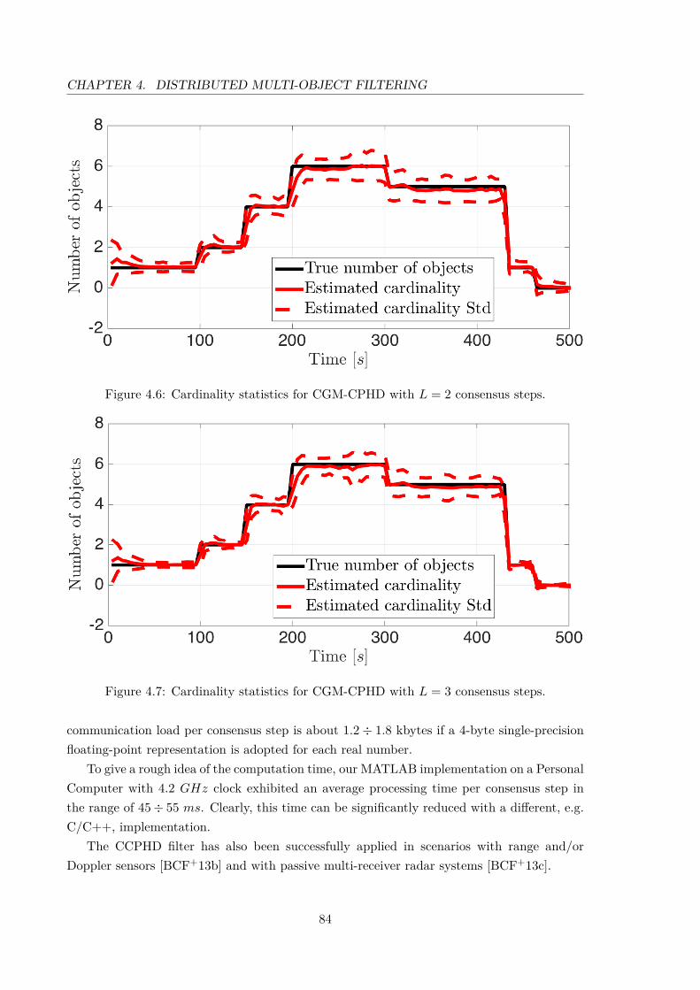
CHAPTER 4. DISTRIBUTED MULTI-OBJECT FILTERING
Figure 4.6: Cardinality statistics for CGM-CPHD with L = 2 consensus steps.
Figure 4.7: Cardinality statistics for CGM-CPHD with L = 3 consensus steps.
communication load per consensus step is about 1.2÷ 1.8 kbytes if a 4-byte single-precisionfloating-point representation is adopted for each real number.
To give a rough idea of the computation time, our MATLAB implementation on a PersonalComputer with 4.2 GHz clock exhibited an average processing time per consensus step inthe range of 45÷ 55 ms. Clearly, this time can be significantly reduced with a different, e.g.C/C++, implementation.
The CCPHD filter has also been successfully applied in scenarios with range and/orDoppler sensors [BCF+13b] and with passive multi-receiver radar systems [BCF+13c].
84

4.3. PERFORMANCE EVALUATION
Figure 4.8: Performance comparison, using OSPA, between GGM-CPHD and CGM-CPHDrespectively with L = 1, L = 2 and L = 3 consensus steps.
Table 4.5: Number of Gaussian components before consensus for CGM-CPHD
TOA1 AVG STD MAX
L = 1 29.39 12.98 63L = 2 10.63 6.97 48L = 3 5.18 4.58 48
TOA2 AVG STD MAX
L = 1 29.34 13.17 66L = 2 10.33 7.11 58L = 3 4.61 4.49 58
TOA3 AVG STD MAX
L = 1 29.08 13.13 63L = 2 10.42 7.06 58L = 3 4.7 4.49 57
TOA4 AVG STD MAX
L = 1 29.72 13.06 67L = 2 10.79 6.97 52L = 3 5.25 4.6 52
DOA1 AVG STD MAX
L = 1 24.12 15 52L = 2 5.65 4.96 53L = 3 4.22 4.25 51
DOA2 AVG STD MAX
L = 1 23.61 15.32 53L = 2 5.6 4.94 50L = 3 4.19 4.24 48
DOA3 AVG STD MAX
L = 1 23.45 15.23 52L = 2 4.92 4.78 58L = 3 4.22 4.35 60
85

CHAPTER 4. DISTRIBUTED MULTI-OBJECT FILTERING
6
×104
54
3
[m]
21
0-1-1
01
2
[m]
34
5
×104
0.2
0.15
0.1
0.05
06
True object
(a) GM before exploiting consensus.
6
×104
54
3
[m]
21
0-1-1
01
2
[m]
34
5
×104
0
0.2
0.4
0.6
0.8
6
True object
(b) GM after the first consensus step (L = 1)
6
×104
54
3
[m]
21
0-1-1
01
2
[m]
34
5
×104
1
0.8
0.6
0.4
0.2
06
True object
(c) GM after the second consensus step (L = 2)
6
×104
54
3
[m]
21
0-1-1
01
2
[m]
34
5
×104
1
0.8
0.6
0.4
0.2
06
True object
(d) GM after the third consensus step (L = 3)
Figure 4.9: GM representation within TOA sensor 1 (see Fig. 2) at the initial time instantthroughout the consensus process. Means and 99.7% confidence ellipses of the Gaussiancomponents of the location PDF are displayed in the horizontal plane while weights of suchcomponents are on the vertical axis.
86

5 Centralizedmulti-object tracking
Contents5.1 The δ-GLMB filter 88
5.1.1 δ-GLMB prediction 885.1.2 δ-GLMB update 89
5.2 GLMB approximation of multi-object densities 905.3 Marginalizations of the δ-GLMB density 915.4 The Mδ-GLMB filter 92
5.4.1 Mδ-GLMB prediction 925.4.2 Mδ-GLMB update 93
5.5 The LMB filter 955.5.1 Alternative derivation of the LMB Filter 955.5.2 LMB prediction 965.5.3 LMB update 97
5.6 Performance evaluation 985.6.1 Scenario 1: radar 1015.6.2 Scenario 2: 3 TOA sensors 101
In this chapter a new approximation of the δ-GLMB filter is presented [FVPV15]. Itwill be shown that the GLMB distribution can be used to construct a principled approx-imation to an arbitrary labeled RFS density that matches the PHD and the cardinalitydistribution [PVV+14]. The resulting filter is referred to as the Marginalized δ-GLMB (Mδ-GLMB) tracking filter since it can be interpreted as a marginalization over the data asso-ciations. The proposed filter is consequently computationally cheaper than the δ-GLMBfilter while still preserving key summary statistics of the multi-object posterior. Impor-tantly, the Mδ-GLMB filter facilitates tractable multi-sensor multi-object tracking. UnlikePHD [VM06], CPHD [VVC07] and Multi-Bernoulli based filters [VVC09], the proposed ap-proximation accommodates statistical dependence between objects. An alternative derivationof the LMB filter proposed in [RVVD14] based on the newly proposed Mδ-GLMB filter ispresented [FVPV15].
87

CHAPTER 5. CENTRALIZED MULTI-OBJECT TRACKING
5.1 The δ-GLMB filter
An efficient approach to multi-object tracking was presented in [VV13] using the δ-GLMBdistribution (2.86) (or equivalently (2.87)), i.e.
π(X) = ∆(X)∑
(I,ξ)∈F(L)×Ξw(I,ξ)δI (L (X))
[p(ξ)
]X, (5.1)
= ∆(X)∑
I∈F(L)δI (L (X))
∑ξ∈Ξ
w(I,ξ)[p(ξ)
]X. (5.2)
The δ-GLMB density naturally arises in multi-object tracking problems when using thestandard detection based measurement model . In the following, the prediction and updatesteps of the δ-GLMB filter is briefly recalled; details can be found in [VV13,VVP14].
5.1.1 δ-GLMB prediction
The standard multi-object dynamic model is described as follows. Given the multi-objectstate Z, each state (ζ, `−) ∈ Z either continues to exist at the next time step with proba-bility PS(ζ, `−) and evolves to a new state (x, `) with probability density ϕk|k−1(x|ζ, `−), ordisappears with probability 1− PS(ζ, `−). Note that the label of the objects is preserved inthe transition, only the kinematic part of state changes. Assuming that Z has distinct labelsand that conditional on Z, the transition of the kinematic states are mutually independent,then the set W of surviving objects at the next time is a labeled multi-Bernoulli RFS [VV13]
fS(W|Z) = ∆(W) ∆(Z) 1L(Z) (L(W)) [Φ (W; ·)]Z , (5.3)
where
Φ(W; ζ, `−) =∑
(x,`)∈Wδ`− (`)PS (ζ, `−) f (x|ζ, `−) +
[1− 1L(W) (`−)
](1− PS (ζ, `−)) . (5.4)
The ∆(Z) in (5.3) ensures that only Z with distinct labels are considered.The set of new objects born at the next time step is distributed according to
fB(Y) = ∆(Y)wB(L(Y)) [pB]Y (5.5)
The birth density fB(·) is defined on X×L and fB(Y) = 0 if Y contains any element x withL(x) /∈ L. The birth model (5.5) includes both labeled Poisson and labeled multi-Bernoullidensities. The multi-object state at the next time X is the superposition of surviving objectsand new born objects, i.e. X = W ∪ Y. Since the label spaces L and B are disjoint, thelabeled birth objects and surviving objects are independent. Thus the multi-object transitiondensity turns out to be the product of the transition density (5.3) and the density of new
88

5.1. THE δ-GLMB FILTER
objects (5.5)f(X|Z) = fS(X ∩ (X× L) |Z) fB (X− (X× L)) . (5.6)
Additional details can be found in [VV13, Subsection IV.D].If the current multi-object prior density is a δ-GLMB of the form (2.86), then the multi-
object prediction density is also a δ-GLMB given by
πk|k−1(X) = ∆(X)∑
(I,ξ)∈F(L)×Ξw
(I,ξ)k|k−1δI (L(X))
[p
(ξ)k|k−1
]X(5.7)
where
w(I,ξ)k|k−1 = wB(I\L−)w(ξ)
S (I ∩ L−) , (5.8)
p(ξ)k|k−1(x, `) = 1L−(`)p(ξ)
S (x, `) + 1B(`)pB(x, `) , (5.9)
p(ξ)S (x, `) =
⟨PS(·, `)ϕk|k−1(x|·, `), p(ξ)
k−1(·, `)⟩
η(ξ)S (`)
, (5.10)
η(ξ)S (`) =
⟨PS(·, `), p(ξ)
k−1(·, `)⟩, (5.11)
w(ξ)S (L) = [η(ξ)
S ]L∑J⊆L−
1J(L)[1− η(ξ)S ]J−Lw(J,ξ)
k . (5.12)
5.1.2 δ-GLMB update
The standard multi-object observation model is described as follows. For a given multi-objectstate X, each state x ∈ X is either detected with probability PD (x) and generates a pointy with likelihood g(y|x), or missed with probability 1 − PD (x), i.e. x generates a BernoulliRFS with parameter (PD(x), g(·|x)). Assuming that conditional on X these Bernoulli RFSsare independent, then the set W ⊂ Y of detected points (non-clutter measurements) is amulti-Bernoulli RFS with parameter set (PD(x), g(·|x)) : x ∈ X. The set C ⊂ Y of falseobservations (or clutter), assumed independent of the detected points, is modeled by a PoissonRFS with intensity function κ(·). The multi-object observation Y is the superposition of thedetected points and false observations, i.e. Y = W ∪ C. Assuming that, conditional on X,detections are independent, and that clutter is independent of the detections, the multi-objectlikelihood is given by
gk(Y |X) = e−〈κ,1〉κY∑
θ∈Θ(L(X))[ψY (·; θ)]X , (5.13)
where Θ(I) is the set of mappings θ : I → 0, 1, ...,M, such that θ(i) = θ(i′) > 0 impliesi = i′, and
ψY (x, `; θ) =
PD(x, `) gk(yθ(`)|x, `)
κ(yθ(`)), if θ(`) > 0
1− PD(x, `) , if θ(`) = 0. (5.14)
89

CHAPTER 5. CENTRALIZED MULTI-OBJECT TRACKING
Note that an association map θ specifies which tracks generated which measurements, i.e.track ` generates measurement yθ(`) ∈ Y , with undetected tracks assigned to 0. The condition“θ(i) = θ(i′) > 0 implies i = i′”, means that a track can generate at most one measurement,and a measurement can be assigned to at most one track, at one time instant. Additionaldetails can be found in [VV13, Subsection IV.C].
If the current multi-object prediction density is also a δ-GLMB of the form (2.86), thenthe multi-object posterior density is a δ-GLMB given by
πk (X) = ∆(X)∑
(I,ξ)∈F(L)×Ξ
∑θ∈Θ(I)
w(I,ξ,θ)k (Yk)δI (L (X))
[p
(ξ,θ)k
]X(5.15)
where Θ(I) denotes the subset of the current maps with domain I, and
w(I,ξ,θ)k (Yk) ∝ w
(I,ξ)k|k−1
[η
(ξ,θ)Yk
(`)]I, (5.16)
η(ξ,θ)Yk
(`) =⟨p
(ξ)k|k−1(·, `), ψYk
(·, `; θ)⟩, (5.17)
p(ξ,θ)k (x, `) =
p(ξ)k|k−1(x, `)ψYk
(x, `; θ)
η(ξ,θ)Yk
(`), (5.18)
ψYk(x, `; θ) =
PD(x, `) g(yθ(`)|x, `)
κ(yθ(`)), if θ(`) > 0
1− PD(x, `) , if θ(`) = 0. (5.19)
Notice that the new association maps θ can be added (stacked) to their respective associationhistories ξ in order to have again the more compact form (2.86) for the updated δ-GLMB(5.15).
5.2 GLMB approximation of multi-object densities
In this section a GLMB approximation of the multi-object density with statistically dependentobjects is proposed. In particular a GLMB density that matches the multi-object density ofinterest in both the PHD and cardinality distribution is derived. The strategy is inspired byMahler’s iid cluster approximation in the CPHD filter [Mah07a], which has proven to be veryeffective in practical multi-object filtering problems [Mah14,GSW09,SWS09]. Moreover, theGLMB approximation captures object dependencies whereas the iid cluster approximationassumes that individual objects are iid from a common single-object density. Proof of theresult is given in the appendix A.
Our result follows from the observation that any labeled RFS density π(·) on F(X×L)can be written as
π(X) = w(L(X))p(X) (5.20)
90

5.3. MARGINALIZATIONS OF THE δ-GLMB DENSITY
where
w(`1, . . . , `n) ,∫π((x1, `1), . . . , (xn, `n))dx1 · · · dxn (5.21)
p((x1, `1), . . . , (xn, `n)) , π((x1, `1), . . . , (xn, `n))w(`1, . . . , `n)
(5.22)
It is implicitly assumed that p(X) is defined to be zero whenever w(L(X)) is zero.Note that since π(·) is symmetric in its arguments, the integral in (5.21) and w is symmet-
ric in `1, . . . , `n. Moreover, since∑L∈F(L)w(L) = 1, w is indeed a probability distribution on
F(L) and can be interpreted as the probability that the labeled RFS has label set `1, . . . , `n.For w(`1, . . . , `n) > 0, p((x1, `1), . . . , (xn, `n)) is the joint probability density (on Xn) ofthe kinematic states x1, . . . , xn given that their corresponding labels are `1, . . . , `n.
Proposition 1 (GLMB approximation).The GLMB that matches the cardinality distribution and the PHD of a labeled RFS withdensity π(·) is given by:
π(X) =∑
I∈F(L)w(I)(L(X))
[p(I)
]X(5.23)
where,
w(I)(L) = δI(L)w(I) (5.24)
p(I)(x, `) = 1I(`)pI\`(x, `) (5.25)
p`1,...,`n(x, `) =∫p((x, `), (x1, `1), . . . , (xn, `n))d (x1, . . . , xn) (5.26)
Remark 13. Note that in [BVV14, Section V] a GLMB was proposed to approximate aparticular family of labeled RFS densities that arises from multi-object filtering with mergedmeasurements. By applying Proposition 1, it can be shown that the approximation usedin [BVV14, Section V] preserves the cardinality distribution and first moment.
Remark 14. In multi-object tracking, the matching of the labeled PHDs d(·, `) and d(·, `)in Proposition 1 is a stronger result than simply matching the unlabeled PHDs alone.
5.3 Marginalizations of the δ-GLMB density
One of the main factors increasing the computational burden of the δ-GLMB filter [VVP14]is the exponential growth of the number of hypotheses in the update of the prior (5.15), whichgives rise to the explicit sum over an association history variable ξ. Further, note that thenumber of association histories is considerably increased in a multi-sensor context. The ideabehind the Mδ-GLMB filter is to construct a principled GLMB approximation π(·) to theposterior density π(·) by means of a marginalization with respect to the association historiesξ. In this section, the time index is dropped for the sake of simplicity and the attention isdevoted to the Mδ-GLMB approximation corresponding to any δ-GLMB density.
91

CHAPTER 5. CENTRALIZED MULTI-OBJECT TRACKING
Proposition 2 (The Mδ-GLMB density).A Marginalized δ-GLMB (Mδ-GLMB) density π(·) corresponding to the δ-GLMB densityπ(·) in (2.86) is a probability density of the form
π(X) = ∆(X)∑
I∈F(L)δI(L(X))w(I)
[p(I)
]X, (5.27)
w(I) =∑ξ∈Ξ
w(I,ξ) , (5.28)
p(I)(x, `) = 1I(`)1w(I)
∑ξ∈Ξ
w(I,ξ)p(ξ)(x, `) . (5.29)
The Mδ-GLMB (5.27) preserves both (labeled) PHD and cardinality distribution of the orig-inal δ-GLMB density π(·) in (2.86).
Note now that the Mδ-GLMB density provided by Proposition 2 is a δ-GLMB whichaggregates the association histories ξ relative to the label set I via (5.28)-(5.29). In fact, themarginalized density (5.27) has no association history set Ξ.
The Mδ-GLMB density can be exploited to construct an efficient recursive multi-objecttracking filter by calculating the Mδ-GLMB approximation step after the δ-GLMB update,and predicting forward in time using the δ-GLMB prediction.
5.4 The Mδ-GLMB filter
The Mδ-GLMB filter propagates a Mδ-GLMB multi-object posterior density forward in timevia the multi-object Bayesian recursion (2.97)-(2.98). Since the Mδ-GLMB is still a δ-GLMB,the equations derived for the δ-GLMB filter [VVP14] as a closed-form solution for the eqs.(2.97)-(2.98) still hold. In the following, the prediction and update steps for the δ-GLMBfilter are briefly recalled; additional details can be found in [VVP14,FVPV15].
5.4.1 Mδ-GLMB prediction
Given the multi-object state Z, each state (ζ, `−) ∈ Z either continues to exist at the nexttime step with probability PS(ζ, `−) and evolves to a new state (x, `) with probability densityϕk|k−1(x|ζ, `−), or dies with probability 1−PS(ζ, `−). The set of newborn objects at the nexttime step is distributed according to the LMB
fB =(r
(`)B , p
(`)B
)`∈B
(5.30)
with L−∩B = ∅ and wB(X) defined in (2.91). The multi-object state at the current time Xk
is the superposition of surviving objects and new born objects.If the current multi-object prior density is a Mδ-GLMB of the form (5.27), then the
92
5.4. THE Mδ-GLMB FILTER
multi-object prediction density is also a Mδ-GLMB given by
πk|k−1(X) = ∆(X)∑
I∈F(L)δI (L (X)) w(I)
k|k−1
[p
(I)k|k−1
]X, (5.31)
where
w(I)k|k−1 = wB(I\L−)w(I)
S (I ∩ L−) , (5.32)
p(I)k|k−1(x, `) = 1L−(`)p(I)
S (x, `) + 1B(`)pB(x, `) , (5.33)
p(I)S (x, `) =
⟨PS(·, `)ϕk|k−1(x|·, `), p(I)
k−1(·, `)⟩
η(I)S (`)
, (5.34)
η(I)S (`) =
⟨PS(·, `), p(I)
k−1(·, `)⟩, (5.35)
w(I)S (L) = [η(I)
S ]L∑J⊆L−
1J(L)[1− η(I)S ]J−Lw(J)
k , (5.36)
which is exactly the δ-GLMB prediction step (5.7) with no association histories from previoustime step, i.e. Ξ = ∅, and with the convention of having the superscript (I) instead of (ξ)due to the marginalization (5.28)-(5.29).
Remark 15. The number of components(w
(I)k+1|k, p
(I)k+1|k
)computed after the Mδ-GLMB
prediction step (5.31) is |F(L0:k+1)|. On the other hand, the number of components(w
(I,ξ)k+1|k,
p(ξ)k+1|k
)after the δ-GLMB prediction (5.7) is |F(L0:k+1)× Ξ| for w(I,ξ)
k+1|k and |Ξ| for p(ξ)k+1|k.
Notice that the number of weights w(I)k+1|k of the Mδ-GLMB is significantly lower than the
w(I,ξ)k+1|k of δ-GLMB. As for the number of location PDFs p(·)
k+1|k, it is worth noticing that thegrowth rate of the association histories ξ ∈ Ξ is super-exponential with time [VV13,VVP14],while the growth rate of the cardinality of F(L0:k+1) is exponential.
The use of the Mδ-GLMB approximation further reduces the number of hypotheses inthe posterior density while preserving the PHD and cardinality distribution. Moreover, theMδ-GLMB is in a form that is suitable for efficient and tractable information fusion (i.e.multi-sensor processing) as will be shown in the next subsection.
5.4.2 Mδ-GLMB update
Given a multi-object state X, each state (x, `) ∈ X is either detected with probability PD (x, `)and generates a measurement y with likelihood gk(y|x, `), or missed with probability 1 −PD(x, `). The multi-object observation Y = y1, . . . , yM is the superposition of the detectedpoints and Poisson clutter with intensity function κ(·).
If the current multi-object prediction density is a Mδ-GLMB of the form (5.27), then themulti-object posterior density is a δ-GLMB given by
πk(X) = ∆(X)∑
I∈F(L)
∑θ∈Θ(I)
δI (L (X))w(I,θ)k (Yk)
[p
(I,θ)k
]X, (5.37)
93

CHAPTER 5. CENTRALIZED MULTI-OBJECT TRACKING
where Θ(I) denotes the subset of the current maps with domain I, and
w(I,θ)k (Yk) ∝ w
(I)k|k−1
[η
(θ)Yk
(`)]I, (5.38)
η(I,θ)Yk
(`) =⟨p
(I)k|k−1(·, `), ψYk
(·, `; θ)⟩, (5.39)
p(I,θ)k (x) =
p(I)k|k−1(x, `)ψYk
(x, `; θ)
η(I,θ)Yk
(`), (5.40)
ψYk(x, `; θ) =
PD(x, `)g(yθ(`)|x, `)
κ(yθ(`)), if θ(`) > 0
1− PD(x, `), if θ(`) = 0. (5.41)
Using (5.28)-(5.29), the Mδ-GLMB density corresponding to the δ-GLMB density in (5.37)is a probability density of the form (5.27) with
w(I)k =
∑θ∈Θ(I)
w(I,θ)k , (5.42)
p(I)k (x, `) = 1I(`)
1w
(I)k
∑θ∈Θ(I)
w(I,θ)k p
(I,θ)k (x, `) . (5.43)
The Mδ-GLMB density provided by (5.42)-(5.43) preserves both PHD and cardinality distri-bution of the original δ-GLMB density.
Remark 16. Each hypothesis I ∈ F (L) generates a set of |Θ(I)| new measurement-to-trackassociation maps for the δ-GLMB posterior. The number of components
(w
(I,θ)k+1|k, p
(I,θ)k+1|k
)stored/computed after the Mδ-GLMB update step (5.37) is |F(L)| ·
∑I∈F(L) |Θ(I)|. On the
other hand, the number of hypotheses(w
(I,ξ,θ)k+1|k , p
(ξ,θ)k+1|k
)after the δ-GLMB update (5.15) is
|F(L)× Ξ|·∑I∈F(L) |Θ(I)| for w(I,ξ,θ)
k+1|k and |Ξ|·∑I∈F(L) |Θ(I)| for p(ξ,θ)
k+1|k. The same conclusionsalong the lines of Remark 15 hold.
Remark 17. After the marginalization procedure (5.42)-(5.43) only |F(L)| hypotheses areretained, as all the new contributions provided by the association maps |Θ(I)| are aggregatedin a single component. Notice that |F(L)| is the same number of hypotheses produced duringthe prediction step (5.31) (see Remark 15). Thus, the prediction step (5.37) sets the upperbound of the hypotheses that will be retained after each full Mδ-GLMB step.
In the multi-sensor setting, for each time instant k, the update step (5.37) (or (5.15) forthe δ-GLMB) is repeatedly evaluated using different measurement sets Y i provided by thesensors i ∈ N (see eq. (2.101)). From Remarks 16 and 17, Mδ-GLMB is preferable to δ-GLMB in terms of memory and computational requirements, since the number of remaininghypotheses after each sensor update step in (2.101) is always set to |F(L)|. Note that thisdoes not apply to δ-GLMB due to the super-exponential memory/computational growthas reported in Remark 15. This is an important property of Mδ-GLMB since it yields aprincipled approximation which greatly decreases the need of pruning hypotheses with respect
94

5.5. THE LMB FILTER
to δ-GLMB [VVP14]. In fact, pruning in the δ-GLMB might lead to poor performance inmulti-sensor scenarios with low SNR (e.g. high clutter intensity, low detection probability,etc.) and limited storage/computational capabilities. For instance, this may happen if asubset of the sensors do not detect one or multiple objects and hypotheses associated tothe true tracks are removed due to pruning. Furthermore, from a mathematical viewpoint,pruning between corrections generally produces a less informative and order-independentapproximation of the posterior distribution in (2.101).
5.5 The LMB filter
The LMB filter introduced in [RVVD14] is a single component approximation of a GLMBdensity (2.77) that matches the unlabeled PHD. An alternative derivation of the LMB ap-proximation (2.90) first proposed in [RVVD14] through a connection with the Mδ-GLMBapproximation is provided hereafter.
5.5.1 Alternative derivation of the LMB Filter
Recall that a LMB density is uniquely parameterized by a set of existence probabilities r(`)
and corresponding track densities p(`)(·):
π(X) = ∆(X) w(L(X))pX (5.44)
where
w(L) =∏ı∈L
(1− r(ı)
) ∏`∈L
1L(`)r(`)
1− r(`) (5.45)
p(x, `) = p(`)(x) (5.46)
By extracting individual tracks from the Mδ-GLMB approximation π(·) (5.27) it is pos-sible to prove that the same expressions for the existence probabilities and state densitiesoriginally proposed for the LMB filter in [RVVD14] can be obtained. In fact
r(`) , Prπ(` ∈ L(X)) (5.47)
=∑`∈L
w(L) (5.48)
=∑
I∈F(L)1I(`)w(L) (5.49)
=∑
I∈F(L)1I(`)w(I) , (5.50)
=∑
(I,ξ)∈F(L)×Ξ1I(`)w(I,ξ) , (5.51)
95

CHAPTER 5. CENTRALIZED MULTI-OBJECT TRACKING
p(`)(x) , Prπ((x, `) ∈ X)Prπ(` ∈ L(X)) (5.52)
=
∫π((x, `) ∪X)δX
r(`) (5.53)
= d(x, `)r(`) , (5.54)
where the notation for the numerator in (5.52) is defined as per [Mah07b, eq. 11.111], whilethe numerator of (5.54) follows from [Mah07b, eq. 11.112]. Notice that the numerator isprecisely the PHD d(·) corresponding to π(·), which by Proposition 1 exactly matches thePHD d(·) corresponding to π(·). It can be easily verified that
d(x, `) =∑
I∈F(L)1I(`)w(I)p(I)(x, `) (5.55)
and consequently
p(`)(x) = 1r(`)
∑I∈F(L)
1I(`)w(I)p(I)(x, `) (5.56)
= 1r(`)
∑(I,ξ)∈F(L)×Ξ
1I(`)w(I,ξ)p(ξ)(x, `) (5.57)
Remark 18. The property of matching the labeled PHD of the δ-GLMB does not hold for theLMB tracking filter, as shown in [RVVD14, Section III], due to the imposed multi-Bernoullistructure for the cardinality distribution. This can be also proved by combining (5.44) withProposition 1, thus showing again that only the unlabeled PHD of the LMB matches exactlythe unlabeled PHD of the original δ-GLMB density.
As suggested by its name, the LMB filter propagates an LMB multi-object posterior den-sity forward in time [RVVD14]. Its recursion will be briefly reviewed in the next subsections.Additional details on its implementation can be found in [RVVD14].
5.5.2 LMB prediction
Given the previous multi-object state Z, each state (ζ, `−) ∈ Z either continues to exist at thenext time step with probability PS(ζ, `−) and evolves to a new state (x, `) with probabilitydensity ϕk|k−1(x|ζ, `−), or dies with probability 1 − PS(ζ, `−). The set of new objects bornat the next time step is distributed according to
fB =(r
(`)B , p
(`)B
)`∈B
(5.58)
with L−∩B = ∅. The multi-object state at the current time Xk is the superposition ofsurviving objects and new born objects.
Suppose that the multi-object posterior density at time k − 1 is LMB with parameter
96

5.5. THE LMB FILTER
set πk−1 =(r(`), p(`)
)`∈L−
. Then, it has been shown in [RVVD14] that the multi-objectpredicted density is also LMB with parameter set
πk|k−1 =(r
(`)S , p
(`)S
)`∈L−
∪(r
(`)B , p
(`)B
)`∈B
, (5.59)
where
r(`)S = ηS(`) r(`) , (5.60)
p(`)S (x) =
⟨PS(·, `)ϕk|k−1(x|·, `), p(·, `)
⟩ηS(`) , (5.61)
ηS(`) = 〈PS(·, `), p(·, `)〉 . (5.62)
5.5.3 LMB update
Given a multi-object state X, each state (x, `) ∈ X is either detected with probability PD (x, `)and generates a measurement y with likelihood gk(y|x, `), or missed with probability 1 −PD(x, `). The multi-object observation Y = y1, ..., yM is the superposition of the detectedpoints and Poisson clutter with intensity function κ(·). Assuming that, conditional on X,detections are independent, and that clutter is independent of the detections, the multi-objectlikelihood is the same of the Mδ-GLMB Update in (5.14).
Suppose that the multi-object predicted density is LMB with parameter set
πk|k−1 =(r
(`)k|k−1, p
(`)k|k−1
)`∈L
. (5.63)
The multi-object posterior density cannot be evaluated in a closed form [RVVD14]. Specif-ically, the LMB πk|k−1 has to be converted to a δ-GLMB density by (possibly) generatingall possible combinations of label sets I ∈ F(L(X)) from the constituent Bernoulli com-ponents [RVVD14]. Further, the δ-GLMB πk|k−1(·) resulting from the conversion processundergoes the δ-GLMB update step (5.15). Finally, the GLMB posterior πk(·) is approxi-mated by an LMB that matches exactly the first moment of the unlabeled posterior intensity.Thus, the updated LMB is given by
πk(X) =(r
(`)k , p
(`)k
)`∈L
, (5.64)
where
r(`)k =
∑(I,θ)∈F(L)×Θ(I)
1I(`)w(I,θ)k (Yk) , (5.65)
p(`)k (x) = 1
r(`)k
∑(I,θ)∈F(L)×Θ(I)
1I(`)w(I,θ)k (Yk) p
(θ)k (x, `) , (5.66)
w(I,θ)(Yk) ∝[η
(θ)Yk
]I ∏`∈L\I
(1− r(`)
k|k−1
)∏i∈I
1L(i)r(i)k|k−1 , (5.67)
97

CHAPTER 5. CENTRALIZED MULTI-OBJECT TRACKING
p(θ)k (x, `) =
pk|k−1(x, `)ψYk(x, `; θ)
η(θ)Yk
(`), (5.68)
η(θ)Yk
(`) =⟨pk|k−1(·, `), ψYk
(·, `; θ)⟩, (5.69)
ψYk(x, `; θ) =
PD(x, `)g(yθ(`)|x, `)
κ(yθ(`)), if θ(`) > 0
1− PD(x, `), if θ(`) = 0. (5.70)
Additional details for an efficient implementation of the LMB filter can be found in [RVVD14].
5.6 Performance evaluation
To assess performance of the proposed Marginalized δ-GLMB (Mδ-GLMB) tracker, a 2-dimensional multi-object tracking scenario is considered over a surveillance area of 50 ×50 [km2]. Two sensor sets are used to represent scenarios with different observability capa-bilities. In particular:
i. a single radar in the middle of the surveillance region is used as it guarantee observ-ability;
ii. a set of 3 range-only (Time Of Arrival, TOA) sensors, deployed as shown in Fig. 5.1, areused as they do not guarantee observability individually, but information from differentsensors need to be combined to achieve it.
The scenario consists of 5 objects as depicted in Fig. 5.2. For the sake of comparison,the Mδ-GLMB is also compared with the δ-GLMB (δ-GLMB) [VV13, VVP14] and LMB(LMB) [RVVD14] filters. The three tracking filters are implemented using Gaussian Mixturesto represent their predicted and updated densities [VVP14,RVVD14]. Due to the non linearityof the sensors, the Unscented Kalman Filter (UKF) [JU04] is exploited to update means andcovariances of the Gaussian components.
The kinematic object state is denoted by x = [px, px, py, py]>, i.e. the planar positionand velocity. The object motion is modeled according to the Nearly-Constant Velocity (NCV)model [FS85,FS86,BSF88,BSL95]:
xk+1 =
1 Ts 0 0
0 1 0 0
0 0 1 Ts
0 0 0 1
xk + wk , Q = σ2
w
14T
4s
12T
3s 0 0
12T
3s T 2
s 0 0
0 0 14T
4s
12T
3s
0 0 12T
3s T 2
s
(5.71)
where: wk is a white noise with zero mean and covariance matrix Q, σw = 5 [m/s2] and thesampling interval is Ts = 5 [s].
98
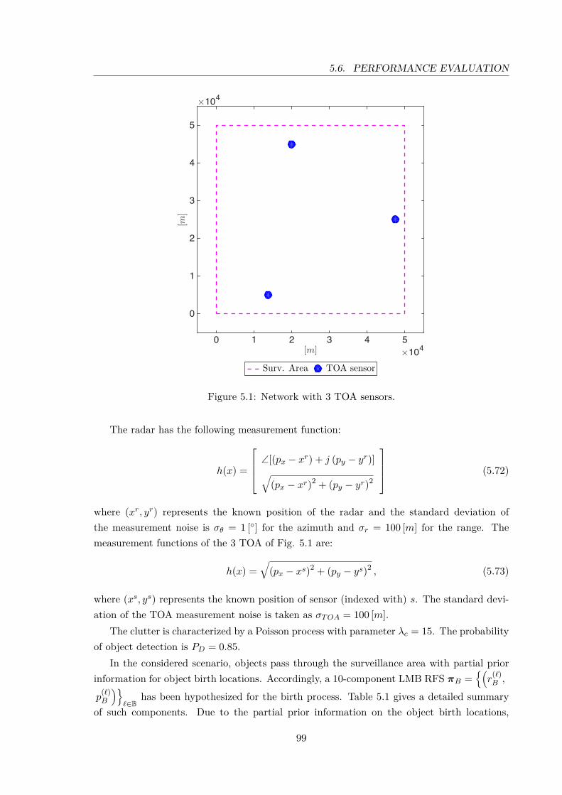
5.6. PERFORMANCE EVALUATION
[m] ×1040 1 2 3 4 5
[m]
×104
0
1
2
3
4
5
Surv. Area TOA sensor
Figure 5.1: Network with 3 TOA sensors.
The radar has the following measurement function:
h(x) =
∠[(px − xr) + j (py − yr)]√(px − xr)2 + (py − yr)2
(5.72)
where (xr, yr) represents the known position of the radar and the standard deviation ofthe measurement noise is σθ = 1 [] for the azimuth and σr = 100 [m] for the range. Themeasurement functions of the 3 TOA of Fig. 5.1 are:
h(x) =√
(px − xs)2 + (py − ys)2 , (5.73)
where (xs, ys) represents the known position of sensor (indexed with) s. The standard devi-ation of the TOA measurement noise is taken as σTOA = 100 [m].
The clutter is characterized by a Poisson process with parameter λc = 15. The probabilityof object detection is PD = 0.85.
In the considered scenario, objects pass through the surveillance area with partial priorinformation for object birth locations. Accordingly, a 10-component LMB RFS πB =
(r
(`)B ,
p(`)B
)`∈B
has been hypothesized for the birth process. Table 5.1 gives a detailed summaryof such components. Due to the partial prior information on the object birth locations,
99

CHAPTER 5. CENTRALIZED MULTI-OBJECT TRACKING
[m] ×1040 1 2 3 4 5
[m]
×104
0
1
2
3
4
5
Object trajectory Surveillance Area
[s]0 200 400 600 800 1000
[m]
×104
0
1
2
3
4
5
[s]0 200 400 600 800 1000
[m]
×104
0
1
2
3
4
5
325
125
225 25 425
630
940
785890555
Figure 5.2: Object trajectories considered in the simulation experiment. The start/end pointfor each trajectory is denoted, respectively, by •\. The ? indicates a rendezvous point.
Table 5.1: Components of the LMB RFS birth process at a given time k.r(`) = 0.09
p(`)B (x) = N
(x; m(`)
B , PB)
PB = diag(106, 104, 106, 104)
Label (k, 1) (k, 2) (k, 3)m
(`)B [0, 0, 40000, 0]> [0, 0, 25000, 0]> [0, 0, 5000, 0]>
Label (k, 4) (k, 5) (k, 6)m
(`)B [5000, 0, 0, 0]> [25000, 0, 0, 0]> [36000, 0, 0, 0]>
Label (k, 7) (k, 8)m
(`)B [50000, 0, 15000, 0]> [50000, 0, 40000, 0]>
Label (k, 9) (k, 10)m
(`)B [40000, 0, 50000, 0]> [10000, 0, 50000, 0]>
some of the LMB components cover a state space region where there is no birth. Cluttermeasurements are, therefore, more prone to generate false objects.
100

5.6. PERFORMANCE EVALUATION
Multi-object tracking performance is evaluated in terms of the Optimal SubPattern Anal-ysis (OSPA) metric [SVV08] with Euclidean distance p = 2 and cutoff c = 600 [m]. Thereported metric is averaged over 100 Monte Carlo trials for the same object trajectories butdifferent, independently generated, clutter and measurement noise realizations. The durationof each simulation trial is fixed to 1000 [s] (200 samples).
The three tracking filters are coupled with the parallel CPHD look ahead strategy describedin [VV13,VVP14]. The CPHD [VVC07] filter.
5.6.1 Scenario 1: radar
Figs. 5.3, 5.4 and 5.5 display the statistics (mean and standard deviation) of the estimatednumber of objects obtained, respectively, with Mδ-GLMB, δ-GLMB and LMB tracking filters.As it can be seen, all the algorithms estimate the object cardinality accurately, with nosubstantial differences. This result implies that, in the presence of a single sensor guaranteeingobservability, the approximations made by both Mδ-GLMB and LMB trackers are not criticalin that they provide performance comparable to δ-GLMB with the advantage of a cheapercomputational burden and reduced storage requirements. Note that the problems introducedby the rendezvous point (e.g. merged or lost tracks) are correctly tackled by all the algorithms.
Fig. 5.6 shows the OSPA distance of the algorithms. Note again that, in agreement withthe estimated cardinality distributions, the OSPA distances are nearly identical.
5.6.2 Scenario 2: 3 TOA sensors
Figs. 5.7, 5.8 and 5.9 display the statistics (mean and standard deviation) of the estimatednumber of objects obtained, respectively, with Mδ-GLMB, δ-GLMB and LMB trackers. TheMδ-GLMB and the δ-GLMB tracking filters estimate the object cardinality accurately, whilethe LMB exhibits poor performance and higher standard deviation due to losing some trackswhen 4 or 5 objects are jointly present in the surveillance area. It is worth noticing that theMδ-GLMB tracker exhibits performance very close to that of δ-GLMB and that the problemsintroduced by the rendezvous point are again succesfully tackled.
Fig. 5.10 shows the OSPA distance. Note that the OSPA of Mδ-GLMB is close to theone of δ-GLMB, while LMB shows an overall higher error in agreement with the cardinalityerror due to losing tracks.
101

CHAPTER 5. CENTRALIZED MULTI-OBJECT TRACKING
Time [s]0 200 400 600 800 1000
Number
ofob
jects
-10123456
True number of objectsEstimated cardinalityEstimated cardinality Std
Figure 5.3: Cardinality statistics for Mδ-GLMB tracking filter using 1 radar.
Time [s]0 200 400 600 800 1000
Number
ofob
jects
-10123456
True number of objectsEstimated cardinalityEstimated cardinality Std
Figure 5.4: Cardinality statistics for δ-GLMB tracking filter using 1 radar.
102

5.6. PERFORMANCE EVALUATION
Time [s]0 200 400 600 800 1000
Number
ofob
jects
-10123456
True number of objectsEstimated cardinalityEstimated cardinality Std
Figure 5.5: Cardinality statistics for LMB tracking filter using 1 radar.
Time [s]0 200 400 600 800 1000
OSPA
[m]
0
100
200
300
400
500
600
GM-δGLMBGM-MδGLMBGM-LMB
Figure 5.6: OSPA distance (c = 600 [m], p = 2) using 1 radar.
103

CHAPTER 5. CENTRALIZED MULTI-OBJECT TRACKING
Time [s]0 200 400 600 800 1000
Number
ofob
jects
-10123456
True number of objectsEstimated cardinalityEstimated cardinality Std
Figure 5.7: Cardinality statistics for Mδ-GLMB tracking filter using 3 TOA.
Time [s]0 200 400 600 800 1000
Number
ofob
jects
-10123456
True number of objectsEstimated cardinalityEstimated cardinality Std
Figure 5.8: Cardinality statistics for δ-GLMB tracking filter using 3 TOA.
104

5.6. PERFORMANCE EVALUATION
Time [s]0 200 400 600 800 1000
Number
ofob
jects
-10123456
True number of objectsEstimated cardinalityEstimated cardinality Std
Figure 5.9: Cardinality statistics for LMB tracking filter using 3 TOA.
Time [s]0 200 400 600 800 1000
OSPA
[m]
0
100
200
300
400
500
600LMBMδ-GLMBδ-GLMB
Figure 5.10: OSPA distance (c = 600 [m], p = 2) using 3 TOA.
105


6 Distributedmulti-object tracking
Contents6.1 Information fusion with labeled RFS 108
6.1.1 Labeled multi-object Kullback-Leibler average 1086.1.2 Normalized weighted geometric mean of Mδ-GLMB densities 1096.1.3 Normalized weighted geometric mean of LMB densities 1106.1.4 Distributed Bayesian multi-object tracking via consensus 111
6.2 Consensus labeled RFS information fusion 1126.2.1 Consensus Mδ-GLMB filter 1126.2.2 Consensus LMB filter 113
6.3 Performance evaluation 1146.3.1 High SNR 1186.3.2 Low SNR 1186.3.3 Low PD 119
The focus of this chapter is on Distributed Multi-Object Tracking (DMOT). We adoptthe RFS formulation since it provides the concept of probability density for multi-object statethat allows us to directly extend existing tools in distributed estimation to the multi-objectcase. Such a concept is not available in the Multiple Hypotheses Tracking (MHT) and JointProbabilistic Data Association (JPDA) approaches [Rei79,FS85,FS86,BSF88,BSL95,BP99].
DMOF based on the RFS paradigm has previously been described in chapter 4 [Mah12,BCF+13a, UCJ13, BCF+14c]. Specifically, an information-theoretic approach to robust dis-tributed multi-object estimation based on the CCPHD filter has been proposed. However,this formulation is not able to provide estimates of the object’s trajectories or tracks.
Taking into account the above-mentioned considerations, the main contributions in thepresent chapter are [FVV+15]:
• the generalization of the robust distributed multi-object filtering approach of subsection4.1.1 to multi-object tracking;
• the development of the Consensus Marginalized δ-Generalized Labeled Multi-Bernoulli(CMδGLMB) and Consensus Labeled Multi-Bernoulli (CLMB) filters as the first dis-tributed multi-object trackers in the RFS framework.
The proposed solutions are based on the concept of labeled RFS introduced in subsection
107

CHAPTER 6. DISTRIBUTED MULTI-OBJECT TRACKING
2.3.6, that enables the estimation of multi-object trajectories in a principled manner [VV13].Moreover, labeled RFS conjugate priors [VV13] have lead to the development of a tractableanalytic multi-object tracking solution called the δ-Generalized Labeled Multi-Bernoulli (δ-GLMB) filter [VVP14]. However, it is not known if this filter is amenable to DMOT. Nonethe-less, the Mδ-GLMB and the LMB filters [FVPV15,RVVD14] are two efficient approximationsof the δ-GLMB filter that
i. have an appealing mathematical formulation that facilitates an efficient and tractableclosed-form fusion rule for DMOT;
ii. preserve key summary statistics of the full multi-object posterior.
In addition, labeled RFS-based trackers do not suffer from the so-called “spooky effect”[FSU09] that degrades the performance in the presence of low detection probability likethe multi-object filters [VVC07,BCF+13a,UCJ13].
6.1 Information fusion with labeled RFS
In this section, the notion of KLA (4.2) introduced in subsection 4.1.1 will be extended todensities of labeled RFSs and will be shown to be equivalent to the normalized weightedgeometric mean. Proofs of the results are provided in the appendix A.
6.1.1 Labeled multi-object Kullback-Leibler average
The benefit of using the RFS framework which provides the concept of probability density ofthe multi-object state, allows us to directly extend the notion of multi-object KLA originallydevised in [BCF+13a] to labeled multi-object densities [FVV+15]. Herewith, we adopt themeasure theoretic notion of multi-object density given in [VSD05], which does not suffer ofthe unit compatibility problem in the integrals involving the product of powers of multi-objectdensities. Note that this density is equivalent to the FISST density as shown in [VSD05].Thus, the standard inner product notation is extended to multi-object densities
〈f , g〉 ,∫f(X) g(X)δX . (6.1)
The weighted KLA fKLA of the labeled multi-object densities f i is defined by
fKLA , arg inff
∑i∈N
ωiDKL
(f ‖ f i
), (6.2)
ωi ≥ 0,∑i∈N
ωi = 1. (6.3)
whereDKL (f ‖ g) ,
∫f(X) logf(X)
g(X) δX (6.4)
is the KLD [Mah03,Mah07b] between two multi-object densities f(·) and g(·).
108

6.1. INFORMATION FUSION WITH LABELED RFS
Theorem 3 (KLA of labeled RFSs).The weighted KLA defined in (6.2) is the normalized weighted geometric mean of the multi-object densities f i(·), i ∈ N , i.e.
fKLA =⊕i∈N
(ωi f i
). (6.5)
Theorem 3 follows from Theorem 1 of [BCF+13a, Section III.B].
Remark 19. The fusion rule (6.5) is the labeled multi-object version of the multi-objectChernoff fusion first proposed by Mahler [Mah00].
Subsequently, it will be shown that the KLAs of Mδ-GLMB and LMB densities are also,respectively, a Mδ-GLMB and an LMB densities. In particular closed-form solutions for thenormalized weighted geometric means are derived. These results are necessary to implementthe fusion rule (6.5) for Mδ-GLMB and LMB tracking filters.
6.1.2 Normalized weighted geometric mean of Mδ-GLMB densities
The following result holds.
Theorem 4 (NWGM of Mδ-GLMB RFSs).Let πı(·), ı = 1, . . . , I, be Mδ-GLMB densities on F(X×L) and ωı ∈ (0, 1), ı = 1, . . . , I, suchthat
∑Iı=1 ω
ı = 1. Then the normalized weighted geometric mean is given by
I⊕ı=1
(ωı πı) (X) = ∆(X)∑
L∈F(L)δL(L(X)) w(L)
[p(L)
]X(6.6)
where
p(L) =
I∏ı=1
(p(L)ı
)ωı
∫ I∏ı=1
(p(L)ı
)ωı
dx
(6.7)
w(L) =
I∏ı=1
(w(L)ı
)ωı[∫ I∏
ı=1
(p(L)ı (x, ·)
)ωı
dx
]L∑F⊆L
I∏ı=1
(w(F )ı
)ωı[∫ I∏
ı=1
(p(F )ı (x, ·)
)ωı
dx
]F (6.8)
The fusion rule for Mδ-GLMBs follows by applying Theorem 4 to find the KLA (6.5) ofthe Mδ-GLMB’s πi(·), i ∈ N . This is summarized in the following Proposition.
Proposition 3 (KLA of Mδ-GLMB RFSs).Suppose that each agent i ∈ N is provided with an Mδ-GLMB πi(·) and that all agents share
109

CHAPTER 6. DISTRIBUTED MULTI-OBJECT TRACKING
the same label space for the birth process, then the Mδ-GLMB components p(L)(·) and w(L)
of the KLA are given by
p(L)(x, `) =⊕i∈N
(ωi p(L)
)(x, `) , (6.9)
w(L) = w(L)∑F⊆L
w(F ) , (6.10)
where
w(L) =∏i∈N
(w
(L)i
)ωi [∫p(L)(x, ·) dx
]L, (6.11)
p(L) =∏i∈N
(p
(L)i
)ωi
. (6.12)
Remark 20. Note that the quantities w(L) and p(L) can be independently determined using(6.9) and (6.10). Thus, the overall fusion procedure is fully parallelizable.
Remark 21. Notice that (6.9) is indeed the CI fusion rule [JU97] for the single-object PDFs.
6.1.3 Normalized weighted geometric mean of LMB densities
The following result holds.
Theorem 5 (NWGM of LMB RFSs).Let πı =
(r
(`)ı , p
(`)ı
)`∈L
, ı = 1, . . . , I, be LMB densities on F(X×L) and ωı ∈ (0, 1),ı = 1, . . . , I, such that
∑Iı=1 ω
ı = 1. Then the normalized weighted geometric mean is givenby
I⊕ı=1
(ωı πı) =(r(`), p(`)
)`∈L
(6.13)
where
r(`) =
∫ I∏ı=1
(r(`)ı p(`)
ı (x))ωı
dx
I∏ı=1
(1− r(`)
ı
)ωı
+∫ I∏
ı=1
(r(`)ı p(`)
ı (x))ωı
dx
(6.14)
p(`) =I⊕ı=1
(ωı p(`)
ı
)(6.15)
The fusion rule for LMBs follows by applying Theorem 5 to find the KLA (6.5) of theLMB’s
(r
(`)i , p
(`)i
)`∈L
, i ∈ N . This is summarized in the following Proposition.
Proposition 4 (KLA of LMB RFSs).Suppose that each agent i ∈ N is provided with an LMB πi(·) and that all agents share the
110

6.1. INFORMATION FUSION WITH LABELED RFS
same label space for the birth process, then the LMB components(r(`), p(`)
)`∈L
of the KLAare given by
r(`) = r(`)
q(`) + r(`) , (6.16)
p(`)(x) =⊕i∈N
(ωi p(`)
i
)(x) , (6.17)
where
r(`) =∫ ∏
i∈N
(r
(`)i p
(`)i (x)
)ωi
dx , (6.18)
q(`) =∏i∈N
(1− r(`)
i
)ωi
. (6.19)
Remark 22. Note that each Bernoulli component(r(`), p(`)
)can be independently deter-
mined using eqs. (6.16) and (6.17). Thus, the overall fusion procedure is fully parallelizable.
Remark 23. Notice that also in this case eq. (6.17) is the CI fusion rule [JU97] for thesingle-object PDFs.
6.1.4 Distributed Bayesian multi-object tracking via consensus
At time k, the global KLA (6.5) which would require all the local multi-object densitiesπik(·), i ∈ N , to be available, can be computed in a distributed and scalable way by iteratingregional averages via the consensus algorithm [BCF+13a, Section III.A] [BC14] described insubsection 2.4.3. Thus, each agent i ∈ N iterates the consensus steps
πik,l =⊕j∈N i
(ωi,j πjk,l−1
), (6.20)
with πik,0(·) = πik(·); ωi,j ≥ 0, satisfying∑j∈N i ωi,j = 1, are the consensus weights relating
agent i to nodes j ∈ N i. Using the same arguments as the single-object case (subsection2.4.3), it follows that, at time k, if the consensus matrix is primitive and doubly stochastic,the consensus iterate of each node in the network converges to the global unweighted KLA(2.107) of the multi-object posterior densities as the number of consensus iterations l tendsto infinity. Convergence follows along the same line as in [CA09, BC14] since F(X× L) is ametric space [Mah07b]. In practice, the iteration is stopped at some finite l.
Remark 24. The consensus iteration (6.20) is the multi-object counterpart of equation(2.119) reviewed in Subsection 2.4.3.
For Mδ-GLMB multi-object densities, (6.20) can be computed via (6.9) and (6.10), whilefor LMB densities by means of (6.16) and (6.17). In the present work, each single-object
111
CHAPTER 6. DISTRIBUTED MULTI-OBJECT TRACKING
density pi is represented by a Gaussian Mixture (GM) of the form
p(x) =NG∑j=1
αj N (x;xj , Pj) . (6.21)
Note that the fusion rules (6.9) and (6.17) involve exponentiation and multiplication of GMin the form of (6.21) which, in general, does not provide a GM. Hence, the same solutionconceived in subsection 4.1.4 for fusing GMs is also adopted here.
The other common approach for representing a single object location PDF p is usingparticles. Information fusion involving convex combinations of Dirac delta functions re-quires, at the best of our knowledge, the exploitation of additional techniques like kerneldensity estimation [UCJ13], least square estimation [HSH+12, OHD14] or parametric modelapproaches [Coa04] which increase the in-node computational burden. Moreover, the localfiltering steps are also more resource demanding with respect to a GM implementation. Atthis stage, it is preferred to follow the approach devised in [BCF+13a] by adopting a GMrepresentation.
6.2 Consensus labeled RFS information fusion
In this section, two novel fully distributed and scalable multi-object tracking algorithms aredescribed by exploiting Propositions 3 and 4 along with consensus [OSFM07,XBL05,CA09,BC14] to propagate information throughout the network [FVV+15]. Pseudo-codes of thealgorithms are also provided.
6.2.1 Consensus Mδ-GLMB filter
This subsection describes the novel Gaussian Mixture - Consensus Marginalized δ-GeneralizedLabelled Multi-Bernoulli (GM-CMδGLMB) filter algorithm. The operations reported in Table6.1 are sequentially carried out locally by each agent i ∈ N of the network. Each nodeoperates autonomously at each sampling interval k, starting from its own previous estimatesof the multi-object distribution πi(·), having location PDFs p(I)(x, `), ∀ ` ∈ I, I ∈ F(L),represented with a GM, and producing, at the end of the sequence of operations, its newmulti-object distribution πi(·) = πiN (·) as an outcome of the Consensus procedure. Thesteps of the GM-CδGLMB algorithm follow hereafter.
1. Each agent i ∈ N locally performs a GM-δGLMB prediction (5.31) and update (5.37).Additional details of the two procedures can be found in [VVP14, Section IV.B].
2. Consensus takes place in each node i involving the subnetwork N i. More precisely,at each consensus step, node i transmits its data to nodes j such that i ∈ N j andwaits until it receives data from j ∈ N i\i. Next, node i carries out the fusion ruleof Proposition 3 over N i, i.e. performs (6.20) using local information and information
112

6.2. CONSENSUS LABELED RFS INFORMATION FUSION
received by N i. Finally, a merging step for each location PDF is applied to reduce thejoint communication-computation burden for the next consensus step. This procedureis repeatedly applied for a chosen number N ≥ 1 of consensus steps.
3. After consensus, an estimate of the object set is obtained from the cardinality PMFand the location PDFs via an estimate extraction described in Table 6.2.
Table 6.1: Gaussian Mixture - Consensus Marginalized δ-Generalized Labeled Multi-Bernoulli(GM-CMδGLMB) filter
procedure GM-CMδGLMB(Node i, Time k)Local Prediction . See (5.31) and [VVP14, Table 2, Section V]
Local Update . See (5.37) and [VVP14, Table 1, Section IV]
Marginalization . See (5.42) and (5.43)
for n = 1, . . . , N doInformation ExchangeGM-MδDGLMB Fusion . See eqs. (6.9) and (6.10)GM Merging . See [VM06, Table II, Section III.C]
end for
Estimate Extraction . See algorithm in Table 6.2end procedure
Table 6.2: GM-CMδGLMB estimate extraction
Input: π, Nmax
Output: Xfor c = 1, . . . , Cmax do
ρ(c) =∑
I∈Fc(L)w(I)
end forC = arg max
cρ(c)
I = arg maxI∈FC(L)
w(I)
X =(x, ˆ)
: ˆ∈ I , x = arg maxx
p(I)(x, ˆ)
6.2.2 Consensus LMB filter
This subsection describes the novel Gaussian Mixture - Consensus Labelled Multi-Bernoulli(GM-CLMB) filter algorithm. The operations reported in Table 6.3 will be sequentiallycarried out locally by each agent i ∈ N of the network. Each node operates autonomouslyat each sampling interval k, starting from its own previous estimates of the multi-objectdistribution πi(·), having location PDFs p(`), ∀ ` ∈ L, represented with a GM, and producing,
113

CHAPTER 6. DISTRIBUTED MULTI-OBJECT TRACKING
at the end of the sequence of operations, its new multi-object distribution πi(·) = πiN (·) as anoutcome of the consensus procedure. A summary description of the steps of the GM-CLMBalgorithm follows.
1. Each agent i ∈ N locally performs a GM-LMB prediction (5.59) and update (5.64). Theupdate procedure involves two more steps: i) a GM δ-GLMB distribution is createdfrom the predicted GM-LMB and updated using the local measurement set Yk; ii) theupdated GM δ-GLMB is converted back to a GM-LMB distribution. The details of theGM-LMB prediction and update can be found in [RVVD14,VVP14].
2. Consensus takes place in each node i involving the subnetwork N i. More precisely,at each consensus step, node i transmits its data to nodes j such that i ∈ N j andwaits until it receives data from j ∈ N i\i. Next, node i carries out the fusion ruleof Proposition 4 over N i, i.e. performs (6.20) using local information and informationreceived by N i. Finally, a merging step for each location PDF is applied to reduce thejoint communication-computation burden for the next consensus step. This procedureis repeatedly applied for a chosen number N ≥ 1 of consensus steps.
3. After consensus, an estimate of the object set is obtained from the cardinality PMFand the location PDFs via an estimate extraction described in Table 6.4.
Table 6.3: Gaussian Mixture - Consensus Labeled Multi-Bernoulli (GM-CLMB) filter
procedure GM-CLMB(Node i, Time k)Local Prediction . See eq. (5.59) and [RVVD14, Proposition 2, Section III.A]
GM-LMB → GM δ-GLMB . See [RVVD14, Section IV.C.1]Local Update . See eq. (5.64) and [VVP14, Table 1, Section IV]GM δ-GLMB → GM-LMB . See [RVVD14, Proposition 4, Section III.B]
for n = 1, . . . , N doInformation ExchangeGM-LMB Fusion . See eqs. (6.16) and (6.17)GM Merging . See [VM06, Table II, Section III.C]
end for
Estimate Extraction . See algorithm in Table 6.4end procedure
6.3 Performance evaluation
To assess performance of the proposed Gaussian Mixture Consensus Marginalized δ-GLMB(GM-CMδGLMB) and LMB (GM-CLMB) described in section 6.2, a 2-dimensional multi-object tracking scenario is considered over a surveillance area of 50 × 50 [km2], wherein the
114

6.3. PERFORMANCE EVALUATION
Table 6.4: GM-CLMB estimate extraction
Input: π =r(`), p(`)
`∈L
, Nmax
Output: Xfor c = 1, . . . , Cmax do
ρ(c) =∑
L∈Fc(L)w(L)
end forC = arg max
cρ(c)
L = ∅for c = 1, . . . , C do
L = L ∪ arg max`∈L\L
r(`)
end for
X =(x, ˆ)
: ˆ∈ L, x = arg maxx
p(ˆ)(x)
sensor network of Fig. 6.1 is deployed. The scenario consists of 5 objects as depicted inFig. 6.2. For the sake of comparison, the trackers are also compared with the Gaussian Mix-ture Consensus CPHD (GM-CCPHD) filter of [BCF+13a] which, however, does not providelabeled tracks.
[m] ×1040 1 2 3 4 5
[m]
×104
0
1
2
3
4
5
Surv. Area TOA sensor DOA sensor Links
Figure 6.1: Network with 7 sensors: 4 TOA and 3 DOA.
115

CHAPTER 6. DISTRIBUTED MULTI-OBJECT TRACKING
[m] ×1040 1 2 3 4 5
[m]
×104
0
1
2
3
4
5
Object trajectory Surveillance Area
[s]0 200 400 600 800 1000
[m]
×104
0
1
2
3
4
5
[s]0 200 400 600 800 1000
[m]
×104
0
1
2
3
4
5
325
125
225 25 425
630
940
785890555
Figure 6.2: Tbject trajectories considered in the simulation experiment. The start/end pointfor each trajectory is denoted, respectively, by •\. The ? indicates a rendezvous point.
The kinematic object state is denoted by x = [px, px, py, py]>, i.e. the planar position andvelocity. The motion of objects is modeled by the filters according to the Nearly-ConstantVelocity (NCV) model [FS85,FS86,BSF88,BSL95]:
xk+1 =
1 Ts 0 0
0 1 0 0
0 0 1 Ts
0 0 0 1
xk + wk , Q = σ2
w
14T
4s
12T
3s 0 0
12T
3s T 2
s 0 0
0 0 14T
4s
12T
3s
0 0 12T
3s T 2
s
, (6.22)
where: wk is a white noise with zero mean and covariance matrix Q, σw = 5 [m/s2] and thesampling interval is Ts = 5 [s].
The sensor network considered in the simulation (see Fig. 6.1) consists of 4 range-only(Time Of Arrival, TOA) and 3 bearing-only (Direction Of Arrival, DOA) sensors characterizedby the following measurement functions:
hi(x) =
∠[(px − xi
)+ j
(py − yi
)], if i is a DOA sensor√
(px − xi)2 + (py − yi)2, if i is a TOA sensor(6.23)
116

6.3. PERFORMANCE EVALUATION
where (xi, yi) represents the known position of sensor i. The standard deviation of DOAand TOA measurement noises are taken respectively as σDOA = 1 [] and σTOA = 100 [m].Because of the non linearity of the aforementioned sensors, the Unscented Kalman Filter(UKF) [JU04] is exploited in each sensor in order to update means and covariances of theGaussian components.
Three different scenarios will be considered, each of which has a different clutter Poissonprocess with parameter λc and a probability of object detection PD.
• High SNR: λc = 5, PD = 0.99. These parameters were used in the work [BCF+13a]and, therefore, will be used as a first comparison test.
• Low SNR: λc = 15, PD = 0.99. These parameters try to describe, in a realistic way,a scenario characterized by high clutter rate λc.
• Low PD: λc = 5, PD = 0.7. These parameters test the distributed algorithms in thepresence of severe misdetection.
All the above-mentioned case studies have, for each sensor, a uniform clutter spatial distri-bution over the surveillance area.
In the considered scenario, objects pass through the surveillance area with partial priorinformation for object birth locations. Accordingly, a 10-component LMB RFS πB =(r
(`)B , p
(`)B
)`∈B
has been hypothesized for the birth process. Table 6.5 gives a detailedsummary of such components. Due to the partial prior information on the object birth lo-
Table 6.5: Components of the LMB RFS birth process at a given time k.r(`) = 0.09
p(`)B (x) = N
(x; m(`)
B , PB)
PB = diag(106, 104, 106, 104)
Label (k, 1) (k, 2) (k, 3)m
(`)B [0, 0, 40000, 0]> [0, 0, 25000, 0]> [0, 0, 5000, 0]>
Label (k, 4) (k, 5) (k, 6)m
(`)B [5000, 0, 0, 0]> [25000, 0, 0, 0]> [36000, 0, 0, 0]>
Label (k, 7) (k, 8)m
(`)B [50000, 0, 15000, 0]> [50000, 0, 40000, 0]>
Label (k, 9) (k, 10)m
(`)B [40000, 0, 50000, 0]> [10000, 0, 50000, 0]>
cations, some of the LMB components cover a state space region where there is no birth.Therefore, clutter measurements are more prone to generate false objects.
Multi-object tracking performance is evaluated in terms of the Optimal SubPattern As-signment (OSPA) metric [SVV08] with Euclidean distance p = 2 and cutoff c = 600 [m]. The
117

CHAPTER 6. DISTRIBUTED MULTI-OBJECT TRACKING
reported metric is averaged over 100 Monte Carlo trials for the same object trajectories butdifferent, independently generated, clutter and measurement noise realizations. The durationof each simulation trial is fixed to 1000 [s] (200 samples).
The GM-CMδGLMB and the GM-CLMB are capped to 20000, 8000 and 3000 hypotheses[VV13, VVP14], respectively, for the High SNR, Low SNR and Low PD scenario, and arecoupled with the parallel CPHD look ahead strategy described in [VV13,VVP14]. The CPHDfilter is similarly capped, for each case study, to the same number of components throughpruning and merging of mixture components.
The parameters of the GM-CCPHD filter have been chosen as follows: the survival prob-ability is Ps = 0.99; the maximum number of Gaussian components is Nmax = 25; themerging threshold is γm = 4; the truncation threshold is γt = 10−4; the extraction thresholdis γe = 0.5; the birth intensity function is the PHD of the LMB RFS of Table 6.5. A singleconsensus step L = 1 is employed for all the simulations.
6.3.1 High SNR
Figs. 6.3, 6.4 and 6.5 display the statistics (mean and standard deviation) of the esti-mated number of objects obtained, respectively, with GM-CCPHD, GM-CLMB and GM-CMδGLMB. As it can be seen, all the distributed algorithms estimate the object cardinalityaccurately, with the GM-CMδGLMB exhibiting better estimated cardinality variance. Notethat the difficulties introduced by the rendezvous point (e.g. merged or lost tracks) arecorrectly tackled by all the distributed algorithms.
Fig. 6.6 shows the OSPA distance for the three algorithms. The improved localizationperformance of GM-CLMB and GM-CMδGLMB is attributed to two factors: (a) the “spookyeffect” [FSU09] causes GM-CCPHD filter to temporarily drop objects which are subjected tomissed detections and to declare multiple estimates for existing tracks in place of the droppedobjects, and (b) the two trackers are generally able to better localize objects due to a moreaccurate propagation of the posterior density. Note that GM-CLMB and GM-CMδGLMBhave similar performance since the approximations introduced by the LMB tracker (see (5.65)-(5.66)) are negligible in the case of high SNR.
6.3.2 Low SNR
Figs. 6.7 and 6.8 display the statistics (mean and standard deviation) of the estimatednumber of objects obtained, respectively, with the GM-CCPHD and the GM-CMδGLMB.As it can be seen, the two distributed algorithms estimate the object cardinality accurately,with the GM-CMδGLMB exhibiting again better estimated cardinality variance.
Note that the GM-CLMB fails to track the objects. The problem is due to the approxi-mation (5.65)-(5.66) made to convert a δ-GLMB to an LMB, becoming significant with lowSNR. In particular, each local tracker fails to properly set the existence probability of thetracks for three main factors: (a) no local observability, (b) high clutter rate and (c) loss of
118

6.3. PERFORMANCE EVALUATION
Time [s]0 200 400 600 800 1000
Number
ofob
jects
-10123456
True number of objectsEstimated cardinalityEstimated cardinality Std
Figure 6.3: Cardinality statistics for the GM-CCPHD filter under high SNR.
Time [s]0 200 400 600 800 1000
Number
ofob
jects
-10123456
True number of objectsEstimated cardinalityEstimated cardinality Std
Figure 6.4: Cardinality statistics for the GM-CLMB tracker under high SNR.
the full posterior cardinality distribution after the probability density conversion. By havinglow existence probabilities, the extraction of the tracks fails even if the single object densitiesare correctly propagated in time.
Fig. 6.9 shows the OSPA distance for the current scenario. As for the previous case study,GM-CMδGLMB outperforms GM-CCPHD.
6.3.3 Low PD
Figs. 6.10 displays the statistics (mean and standard deviation) of the estimated number ofobjects obtained with the GM-CMδGLMB. It is worth pointing out that the only working
119

CHAPTER 6. DISTRIBUTED MULTI-OBJECT TRACKING
Time [s]0 200 400 600 800 1000
Number
ofob
jects
-10123456
True number of objectsEstimated cardinalityEstimated cardinality Std
Figure 6.5: Cardinality statistics for the GM-CMδGLMB tracker under high SNR.
Time [s]0 200 400 600 800 1000
OSPA
[m]
0
100
200
300
400
500
600GM-CCPHDGM-CLMBGM-CMδGLMB
Figure 6.6: OSPA distance (c = 600 [m], p = 2) under high SNR.
distributed algorithm is, indeed, the GM-CMδGLMB and that it exhibits good performancein terms of average number of estimated objects in a very tough scenario with PD = 0.7.
Fig. 6.11 shows the OSPA distance for the current scenario.
120

6.3. PERFORMANCE EVALUATION
Time [s]0 200 400 600 800 1000
Number
ofob
jects
-10123456
True number of objectsEstimated cardinalityEstimated cardinality Std
Figure 6.7: Cardinality statistics for the GM-CCPHD filter under low SNR.
Time [s]0 200 400 600 800 1000
Number
ofob
jects
-10123456
True number of objectsEstimated cardinalityEstimated cardinality Std
Figure 6.8: Cardinality statistics for the GM-CMδGLMB tracker under low SNR.
Time [s]0 200 400 600 800 1000
OSPA
[m]
0
100
200
300
400
500
600GM-CCPHDGM-CMδGLMB
Figure 6.9: OSPA distance (c = 600 [m], p = 2) under low SNR.
121

CHAPTER 6. DISTRIBUTED MULTI-OBJECT TRACKING
Time [s]0 200 400 600 800 1000
Number
ofob
jects
-10123456
True number of objectsEstimated cardinalityEstimated cardinality Std
Figure 6.10: Cardinality statistics for the GM-CMδGLMB tracker under low PD.
Time [s]0 200 400 600 800 1000
OSPA
[m]
0
100
200
300
400
500
600
GM-CMδGLMB
Figure 6.11: OSPA distance (c = 600 [m], p = 2) under low PD.
122

7 Conclusions and futurework
The present dissertation has summarized the work carried out during my 3-year Ph.D. re-search work in the field of distributed filtering and tracking. Contributions have spannedfrom single-object to multi-object scenarios, in both centralized and distributed settings. Inparticular, distributed tracking over sensor networks requires redesigning the architectureand algorithms to address the following issues:
1. lack of a central fusion node;
2. scalable processing with respect to the network size;
3. each node operates without knowledge of the network network topology;
4. each node operates without knowledge of the dependence between its own informationand the information received from other nodes.
Four main ingredients have been considered in order to provide novel research contributions.
i. The Bayesian framework for modeling the quantities to be estimated as random vari-ables characterized by Probability Density Functions (PDFs), and for providing animproved estimation of such quantities by conditioning the PDF on the available noisymeasurements.
ii. The Random Finite Set (RFS) formulation as it provides the concept of probabilitydensity of the multi-object state that allows us to directly generalize single-object esti-mation to the multi-object case.
iii. The Kullback-Leibler Average (KLA) as a sensible information-theoretic definition forconsistently fusing PDFs of the quantity to be estimated provided by different nodes(or agents).
iv. Consensus as a tool for developing scalable and reliable distributed fusion techniquesover a network where each agent aims to compute the collective average of a givenquantity by iterative regional averages, where the terms “collective” and “regional”mean “over all network nodes” and, respectively, “over neighboring nodes only”.
123

CHAPTER 7. CONCLUSIONS AND FUTURE WORK
The main contributions of the present thesis are herewith summarized.
A novel distributed single-object filter, namely Parallel Consensus on Likelihoods andPriors (CLCP). The proposed algorithm is based on the idea of carrying out, in par-allel, a separate consensus for the novel information (likelihoods) and one for the priorinformation (priors). This parallel procedure is conceived as an improvement of theConsensus on Posteriors (CP) approach to avoid underweighting the novel informationduring the fusion steps. The outcomes of the two consensuses are then combined toprovide the fused posterior density.
Two novel consensus Multiple Model (MM) filters to be used for tracking a maneuveringobject, namely Distributed First Order Generalized Pseudo-Bayesian (DGPB1) andDistributed Interacting Multiple Model (DIMM) filters.
A novel result on Distributed Multi-Object Filtering (DMOF) over a sensor networkusing RFSs. Specifically, a generalisation of the single-object Kullback-Leibler Average(KLA) to the RFS framework has been devised.
A novel consensus multi-object filter, the Consensus Cardinalized Probability HypothesisDensity (CCPHD) filter. Each tracking agent locally updates multi-object CPHD, i.e.the cardinality distribution and the PHD, exploiting the multi-object dynamics and theavailable local measurements, exchanges such information with communicating agentsand then carries out a fusion step to combine the information from all neighboringagents.
A novel approximation of the δ-GLMB filter, namely the Marginalized δ-Generalised La-beled Multi-Bernoulli (Mδ-GLMB). The result is based on a principled Generalised La-beled Multi-Bernoulli (GLMB) approximation of the labeled RFS posterior that matchesexactly the posterior PHD and cardinality distribution. The proposed approximationcan be interpreted as performing a marginalization with respect to the association his-tories arising from the δ-GLMB filter. The key advantage of the new filter lies in thereduced growth rate of the number of new components generated at each filtering step.In particular, the approximation (or marginalization) step performed after each updateis guaranteed to reduce the number of generated components which normally arise frommultiple measurement-to-track association maps. Typically, the proposed Mδ-GLMBfilter requires much less computation and storage especially in multi-sensor scenarioscompared to the δ-GLMB filter. Furthermore the proposed Mδ-GLMB filter inheritsthe same implementation strategies and parallelizability of the δ-GLMB filter.
The generalisation of the KLA to labeled RFSs.
Two novel consensus tracking filters, namely a Consensus Marginalized δ-GeneralizedLabeled Multi-Bernoulli (CMδGLMB) and Consensus Labeled Multi-Bernoulli (CLMB)
124

tracking filter. The proposed algorithms provide fully distributed, scalable and compu-tationally efficient solutions for multi-object tracking.
From the above-mentioned contributions, the following conclusions can be drawn.
. The KLA turns out to be an effective information-theoretic approach for distributinginformation over a sensor network.
. Consensus algorithms can be exploited so as to fuse, in a fully distributed and scal-able fashion, the information collected from multiple sensors which are supposed to beheterogeneous and geographically dispersed.
. The CLCP has proven to be a reliable distributed filter. Its performance is crucially de-pendant on the choice of a suitable weight of the innovation (likelihood) term combinedwith the prior. In particular, the choice of such a weight equal to the (usually unknown)number of nodes provides the best performance when the number of consensus steps issufficiently large, but for very few consensus steps can be improved resorting to othersimple choices, proposed in this thesis work, which do not require knowledge of thenetwork size.
. The DGPB1 and DIMM have been proven to be capable of tracking a highly-maneuveringobject with a network consisting of range-only and angle-only sensors along with com-munication nodes. DIMM performs significantly better than DGPB1 when a turn isapproaching.
. The multi-object KLA in the RFS framework turns out to be a significant contributionin the field of distributed multi-object filtering. The proposed consensus algorithmadmits an intuitive interpretation in terms of distributed averaging of the local multi-object densities. Its formulation has led to the development of the CCPHD filter whichproved its effectiveness in a realistic simulation scenario.
. The labeled RFS approach turns out to be a strong mathematical tool for modeling theprobability density of a multi-object state. Its key features allow to directly generalise,in a rigorous and elegant way, the multi-object KLA to the broader labeled multi-objectcase.
. The Mδ-GLMB provides an excellent tradeoff between computational/storage require-ments and performance for multi-object tracking. Moreover, it has an appealing math-ematical formulation which 1) facilitates an efficient and tractable closed-form solutionfor distributed multi-object tracking and 2) preserves key summary statistics of the fullmulti-object posterior.
. The CLMB fails to track objects in low SNR scenarios. The problem is due to theapproximation made to convert a δ-GLMB into an LMB, becoming significant with
125

CHAPTER 7. CONCLUSIONS AND FUTURE WORK
low SNR. In particular, each local tracking filter fails to properly set the existenceprobability of the tracks in the case of having: 1) no local observability, 2) high clutterrate and 3) loss of the full posterior cardinality distribution after the probability densityconversion. By having low existence probabilities, the extraction of the tracks fails evenif the single object densities are correctly propagated in time.
Based on the above achievements, possible future work will concern the following issues.
To consider sensors with different field-of-view to cope with real-world sensor capabili-ties. So far, it has been assumed that the area subjected to surveillance is exactly theintersection of the sensor fields-of-view, or that each sensor field-of-view is exactly thesurveillance region. By a practical viewpoint this issue needs to be addressed. Thus,the proposed algorithms will have to take into account a state-dependent probabilityof detection instead of a constant one as assumed in the present work. Moreover, thefusion techniques will have to be redesigned to consider the above-mentioned context.
To investigate distributed measurement-driven object initialization. The object birthprocess of the RFS filtering approach is capable of accounting for a large variety of sce-narios in which object birth locations could also be unknown. However, a measurement-driven approach would be much more effective compared to a static birth process. Theinformation provided by the sensors could be used to dynamically accommodate eachsensor birth process. Thus, a more complete picture of newborn objects could beachieved by fusing local information with the one provided by the other nodes.
126

A Proofs
Proof of Theorem 1:The cost to be minimized by the KLA is
J (µ) =∑i∈N
πiDKL
(µ ‖ µi
)=∑i∈N
πi∑j∈R
µj log(µj
µi,j
)
=∑j∈R
µj∑i∈N
πi log(µi
µi,j
)
=∑j∈R
µj∑i∈N
log(µj
µi,j
)πi
=∑j∈R
µj log(∏i∈N
(µj)πi
(µi,j)πi
)
=∑j∈R
µj log
µj∏i∈N
(µi,j
)πi
where the relationship
∑i∈N πi = 1 has been exploited. Let µ be defined as in (3.24), then
J(µ) =∑j∈R
µj log(µj
c µj
)(A.1)
where c ,∑h∈R
∏i∈N
(µi,h
)πi
. Hence
J (µ) = DKL (µ ‖ µ)− log c (A.2)
where the relationship∑j∈R µj = 1 has been exploited. Then the infimum of J (µ), i.e. the
weighted KLA of (3.23), is just provided by µ = µ as in (3.24).
127

APPENDIX A. PROOFS
Proof of Theorem 2:Let
f(X) =∏i
[f i(X)
]ωi (A.3)
c =∫f(X)δX , (A.4)
so that the fused multi-object density in (4.4) can be expressed as f(X) = f(X)/c. Then,the cost to be minimized by the KLA is
J(f) =∑i
ωiDKL
(f ‖ f i
)=∑i
ωi
∫f (X) log
(f(X)f i(X)
)δX
=∑i
ωi
∞∑n=0
1n!
∫f (x1, . . . , xn) log
(f (x1, . . . , xn)f i (x1, . . . , xn)
)dx1 · · · dxn
=∞∑n=0
1n!
∫f (x1, . . . , xn)
∑i
ωi log(f (x1, . . . , xn)f i (x1, . . . , xn)
)dx1 · · · dxn
=∞∑n=0
1n!
∫f (x1, . . . , xn) log
f (x1, . . . , xn)∏i
[f i (x1, . . . , xn)
]ωi
dx1 · · · dxn
=∞∑n=0
1n!
∫f (x1, . . . , xn) log
(f (x1, . . . , xn)f (x1, . . . , xn)
)dx1 · · · dxn
=∞∑n=0
1n!
∫f (x1, . . . , xn) log
(f (x1, . . . , xn)c · f (x1, . . . , xn)
)dx1 · · · dxn
=∞∑n=0
1n!
∫f (x1, . . . , xn) log
(f (x1, . . . , xn)f (x1, . . . , xn)
)dx1 · · · dxn+
−∞∑n=0
1n!
∫f (x1, . . . , xn) log(c) dx1 · · · dxn
=∫f (X) log
(f(X)f(X)
)δX − log(c)
∫f(X)δX
= DKL
(f ‖ f
)− log(c)
Since the KLD is always nonnegative and is zero if and only if its two arguments coincidealmost everywhere, the above J(f) is trivially minimized by fKLA(X) defined as in (4.4).
Proof of Proposition 1:First, the cardinality distributions of π(·) and π(·) are proven to be the same. Following
128

(2.81), the cardinality distribution of the GLMB in (5.23) is given by:
ρ(n) =∑
L∈Fn(L)
∑I∈F(L)
w(I)(L) (A.5)
=∑
L∈Fn(L)w(L) (A.6)
= 1n!
∑(`1,...`n)∈Ln
w(`1, . . . , `n) (A.7)
= 1n!
∑(`1,...`n)∈Ln
∫π ((x1, `1), . . . , (xn, `n)) dx1 · · · dxn (A.8)
= 1n!
∫π (x1, . . . ,xn)) dx1 · · · dxn (A.9)
= ρ(n) (A.10)
Second, the PHD corresponding to π(·) and π(·) are proven to be the same. Note from thedefinition of p(I)(x, `) that
p(`,`1,...,`n)(x, `) = 1`,`1,...,`n(`)p`1,...,`n(x, `) (A.11)
=∫p( (x, `), (x1, `1), . . . , (xn, `n))dx1 · · · dxn (A.12)
Substituting the GLMB density (5.23) into the PHD of the object with label (or track) `yields
d(x, `) =∫π((x, `) ∪X) δX (A.13)
from which
d(x, `) =∫ ∑
I∈F(L)w(I) (L((x, `) ∪X)) [p(I)](x,`)∪XδX (A.14)
=∑
I∈F(L)
[∫w(I) (` ∪ L(X)) [p(I)]XδX
]p(I)(x, `) (A.15)
=∑
I∈F(L)
∑L∈F(L)
w(I) (` ∪ L)[p(I)(·, `)dx
]Lp(I)(x, `) (A.16)
where the last step follows from Lemma 3 in [VV13, Section III.B]. Noting that p(I)(·, `) isa probability density, and using (5.24) gives
d(x, `) =∑
L∈F(L)
∑I∈F(L)
δI (` ∪ L)w(I)p(I)(x, `) (A.17)
=∑
L∈F(L)w (` ∪ L) p(`∪L)(x, `) (A.18)
=∞∑n=0
1n!
∑(`1,...,`n)∈Ln
w (`, `1, . . . `n) p(`,`1,...`n)(x, `) (A.19)
129

APPENDIX A. PROOFS
from which by applying (A.12), we obtain:
d(x, `) =∞∑n=0
1n!
∑(`1,...,`n)∈Ln
w (`, `1, . . . `n)∫p ((x, `), (x1, `1), . . . , (xn, `n)) dx1 · · · dxn
(A.20)
=∫π((x, `) ∪X)δX (A.21)
= d(x, `) . (A.22)
Proof of Proposition 2:We apply the result in Proposition 1 which can be used to calculate the parameters of themarginalized δ-GLMB density. Notice that such a result applies to any labeled RFS densityand our first step is to rewrite the δ-GLMB density (2.86) in the general form for a labeledRFS density [PVV+14], i.e.
π(X) = w(L(X))p(X) (A.23)
where
w(`1, . . . , `n) ,∫Xnπ((x1, `1), . . . , (xn, `n))d(x1, . . . , xn) (A.24)
=∑
I∈F(L)δI(`1, . . . , `n)
∑ξ∈Ξ
w(I,ξ)∫Xnp(ξ)(x1, `1) · · · p(ξ)(xn, `n)dx1 · · · dxn
(A.25)
=∑ξ∈Ξ
w(`1,...,`n,ξ)∑
I∈F(L)δI(`1, . . . , `n) (A.26)
=∑ξ∈Ξ
w(`1,...,`n,ξ) (A.27)
and
p((x1, `1), . . . , (xn, `n)) , π((x1, `1), . . . , (xn, `n))w(`1, . . . , `n)
(A.28)
= ∆((x1, `1), . . . , (xn, `n)) 1w(`1, . . . , `n)
·
·∑
I∈F(L)δI (`1, . . . , `n)
∑ξ∈Ξ
w(I,ξ)[p(ξ)
](x1,`1),...,(xn,`n).(A.29)
Applying Proposition 1, the parameters w(I) and p(I)(·) for the Mδ-GLMB approximationthat match the cardinality and PHD are
w(I)(L) = δI(L)w(I) = δI(L)∑ξ∈Ξ
w(I,ξ) (A.30)
130

and
p(I)(x, `) = 1I(`)pI−`(x, `) (A.31)
= 1I(`)∫p((x, `), (x1, `1), . . . , (xj , `j))d(x1, . . . , xj) (A.32)
where I\` = `1, . . . , `j. Substituting the expression (A.29) in (A.32), we have
p(I)(x, `) = 1I(`) ∆((x, `), (x1, `1), . . . , (xj , `j))1
w(`, `1, . . . , `j)·
·∑
J∈F(L)δJ (`, `1, . . . , `j)
∑ξ∈Ξ
w(J,ξ)∫ [
p(ξ)](x,`),(x1,`1),...,(xj ,`j)
d(x1, . . . , xj)
(A.33)
= 1I(`) ∆((x, `), (x1, `1), . . . , (xj , `j))1
w(`, `1, . . . , `j)·∑
J∈F(L)δJ (`, `1, . . . , `j)
∑ξ∈Ξ
w(J,ξ)p(ξ)(x, `) (A.34)
and, noting that I = `, `1, . . . , `j, it follows that only one term in the sum over J is non-zerothus giving
p(I)(x, `) = 1I(`)∆((x, `), (x1, `1), . . . , (xj , `j))1∑
ξ∈Ξw(I,ξ)
∑ξ∈Ξ
w(I,ξ)p(ξ)(x, `) (A.35)
Consequently, the Mδ-GLMB approximation is given by
π(X) =∑
I∈F(L)w(I)(L(X))
[p(I)
]X(A.36)
= ∆(X)∑
I∈F(L)δI(L(X))
∑ξ∈Ξ
w(I,ξ)
1I(·)1∑
ξ∈Ξw(I,ξ)
∑ξ∈Ξ
w(I,ξ)p(ξ)(·, ·)
X
(A.37)
= ∆(X)∑
I∈F(L)δI(L(X))w(I)
[p(I)
]X(A.38)
where
w(I) =∑ξ∈Ξ
w(I,ξ) (A.39)
p(I)(x, `) = 1I(`)1∑
ξ∈Ξw(I,ξ)
∑ξ∈Ξ
w(I,ξ)p(ξ)(x, `) (A.40)
= 1I(`)1w(I)
∑ξ∈Ξ
w(I,ξ)p(ξ)(x, `) (A.41)
131

APPENDIX A. PROOFS
Proof of Theorem 4:For the sake of simplicity, let us consider only two Mδ-GLMB densities ı ∈ 1, 2. From (6.6)one gets
π(X) = 1K
∆(X)∑
L∈F(L)δL(L(X)) w(L)
1
[p
(L)1
]Xω ∆(X)∑
L∈F(L)δL(L(X)) w(L)
2
[p
(L)2
]X1−ω
.
(A.42)Notice that the exponentiation of a sum of delta functions is a sum of the exponentiateddelta function terms, i.e
π(X)ω =
∆(X)
(w(L1)
)ω [(p(L1)
)ω]Xif L(X) = L1
......
∆(X)(w(Ln)
)ω [(p(Ln)
)ω]Xif L(X) = Ln
Thus, (A.42) yields:
π(X) = ∆(X)K
∑L∈F(L)
δL(L(X))(w
(L)1
)ω (w
(L)2
)1−ω[(p
(L)1
)ω (p
(L)2
)1−ω]X
(A.43)
= ∆(X)K
∑L∈F(L)
δL(L(X))(w
(L)1
)ω (w
(L)2
)1−ω[∫ (
p(L)1 (x, ·)
)ω (p
(L)2 (x, ·)
)1−ω]L·
·[(ω p(L)
1
)⊕((1− ω) p(L)
2
)]X. (A.44)
The normalization constant K can be easily evaluated exploiting Lemma 3 of [VV13, SectionIII.B], i.e.
K =∫
∆(X)∑
L∈F(L)δL(L(X))
(w
(L)1
)ω (w
(L)2
)1−ω[(p
(L)1
)ω (p
(L)2
)1−ω]X
δX (A.45)
=∑L⊆L
(w
(L)1
)ω (w
(L)2
)1−ω[∫ (
p(L)1
)ω (p
(L)2 (x, ·)
)1−ωdx
]L. (A.46)
Applying (A.46) in (A.44) one has
p(L) =[(ω p(L)
1
)⊕((1− ω) p(L)
2
)]X(A.47)
w(L) =
(w
(L)1
)ω (w
(L)2
)1−ω[∫ (
p(L)1 (x, ·)
)ω (p
(L)2 (x, ·)
)1−ω]L
∑F⊆L
(w
(F )1
)ω (w
(F )2
)1−ω[∫ (
p(F )1 (x, ·)
)ω (p
(F )2 (x, ·)
)1−ω]F
(A.48)
It can be proved by induction that Theorem 4 holds considering I Mδ-GLMB densities instead
132

of 2.
Proof of Proposition 3:The proof readily follows by noting that the KLA (6.5) can be evaluated using (6.6) ofTheorem 4.
The following Lemma is useful to prove Theorem 5.
Lemma 1 (Normalization constant of LMB KLA).Let π1(X) =
(r
(`)1 , p
(`)1
)`∈L
and π2(X) =(r
(`)2 , p
(`)2
)`∈L
be two LMB densities on X×Land ω ∈ (0, 1) then
K ,∫π1(X)ωπ2(X)1−ωδX (A.49)
=⟨ω π1, (1− ω) π2
⟩(A.50)
=(q(·) + r(·)
)L. (A.51)
Proof of Lemma 1:We make use of the Binomial Theorem [AS64] which states
∑L⊆L
fL = (1 + f)L (A.52)
Applying Lemma 3 of [VV13, Section III.B] to the definition (A.49) of K gives
K =(q(·))L ∑
L⊆L
(r(·)
q(·)
)L. (A.53)
Applying (A.52) to (A.53) gives
K =(q(·))L(
1 + r(·)
q(·)
)L
(A.54)
=(q(·) + r(·)
)L(A.55)
having defined
r(`) ,∫ (
r(`)1 p
(`)1 (x)
)ω (r
(`)2 p
(`)2 (x)
)1−ωdx, (A.56)
q(`) ,(1− r(`)
1
)ω (1− r(`)
2
)1−ω. (A.57)
Proof of Theorem 5:For the sake of simplicity, let us consider only two LMB densities ı ∈ 1, 2. From (6.13) one
133

APPENDIX A. PROOFS
gets
π(X) = 1K
[∆(X)w1(L(X))pX
1
]ω [∆(X)w2(L(X))pX
2
]1−ω(A.58)
= ∆(X)K
(q(·))L 1L(·)
(r
(·)1
1− r(·)1
)ω (r
(·)2
1− r(·)2
)1−ωL(X) (pω1 p
1−ω2
)X(A.59)
= ∆(X)K
(q(·))L 1L(·)
(r
(·)1
1− r(·)1
)ω (r
(·)2
1− r(·)2
)1−ω ∫pω1 p
1−ω2 dx
L(X)
·
· [(ω p1)⊕ ((1− ω) p2)]X (A.60)
Hence, recalling definitions (A.56) and (A.57), one has
w(L) =
(q(·))L(
1L(·) r(·)
q(·)
)L(q(·) + r(·))L (A.61)
=(
q(·)
q(·) + r(·)
)L\L( 1L(·) r(·)
q(·) + r(·)
)L(A.62)
=(
q(·)
q(·) + r(·)
)L(1L(·) r
(·)
q(·)
)L, (A.63)
p(`)(x) =[(ω p(`)
1
)⊕((1− ω) p(`)
2
)]X. (A.64)
It follows from (A.62) that q(`) + r(`) = 1, ∀ ` ∈ L, where
r(`) = r(`)
q(`) + r(`) (A.65)
q(`) = q(`)
q(`) + r(`) . (A.66)
It can be proved by induction that Theorem 5 holds considering I LMB densities instead of2.
Proof of Proposition 4:The proof readily follows by noting that the KLA (6.5) can be evaluated using (6.13) ofTheorem 5.
134

Bibliography
[AF70] G. Ackerson and K. S. Fu, “On state estimation in switching environments,”IEEE Trans. on Automatic Control, vol. 15, no. 1, pp. 10–17, 1970.
[Aka98] H. Akaike, “Information theory and the extension of the maximum likelihoodprinciple,” in Selected Papers of Hirotugu Akaike. Springer New York, 1998, pp.199–213.
[AM12] B. Anderson and J. B. Moore, Optimal filtering. Courier Dover Publications,2012.
[AS64] M. Abramowitz and I. A. Stegun, Handbook of mathematical functions: withformulas, graphs, and mathematical tables. Washington, DC: National Bureauof Standards, 1964. [Online]. Available: http://people.math.sfu.ca/∼cbm/aands/abramowitz and stegun.pdf
[BBS88] H. Blom and Y. Bar-Shalom, “The interacting multiple model algorithm for sys-tems with Markovian switching coefficients,” IEEE Trans. on Automatic Control,vol. 33, no. 8, pp. 780–783, 1988.
[BC14] G. Battistelli and L. Chisci, “Kullback-Leibler average, consensus on probabilitydensities, and distributed state estimation with guaranteed stability,” Automat-ica, vol. 50, no. 3, pp. 707–718, 2014.
[BCF+13a] G. Battistelli, L. Chisci, C. Fantacci, A. Farina, and A. Graziano, “ConsensusCPHD filter for distributed multitarget tracking,” IEEE Journal of Selected Top-ics in Signal Processing, vol. 7, no. 3, pp. 508–520, 2013.
[BCF+13b] ——, “Distributed multitarget tracking with range-Doppler sensors,” in Proc.21st European Signal Processing Conference (EUSIPCO), pp. 1-5, Marrakech,Morocco, 2013.
[BCF+13c] ——, “Distributed multitarget tracking for passive multireceiver radar systems,”in Proc. 14th International Radar Symposium (IRS), pp. 337-342, Dresden, Ger-many, 2013.
[BCF+13d] ——, “Distributed tracking with Doppler sensors,” in Proc. 52nd IEEE Conf. onDecision and Control (CDC), pp. 4760-4765, Florence, Italy, 2013.
[BCF14a] G. Battistelli, L. Chisci, and C. Fantacci, “Parallel consensus on likelihoods andpriors for networked nonlinear filtering,” IEEE Signal Processing Letters, vol. 21,no. 7, pp. 787–791, 2014.
135

BIBLIOGRAPHY
[BCF+14b] G. Battistelli, L. Chisci, C. Fantacci, A. Farina, and A. Graziano, “Consensus-based multiple-model Bayesian filtering for distributed tracking,” IET Radar,Sonar & Navigation, DOI: 10.1049/iet-rsn.2014.0071, 2014.
[BCF+14c] G. Battistelli, L. Chisci, C. Fantacci, N. Forti, A. Farina, and A. Graziano, “Dis-tributed peer-to-peer multitarget tracking with association-based track fusion,”in Proc. 17th Int. Conf. on Information Fusion (FUSION), Salamanca, Spain,2014.
[BCMP11] G. Battistelli, L. Chisci, S. Morrocchi, and F. Papi, “An information-theoreticapproach to distributed state estimation,” in Proc. 18th IFAC World Congress,pp. 12477-12482, Milan, Italy, 2011.
[BJA12] T. Bailey, S. Julier, and G. Agamennoni, “On conservative fusion of informationwith unknown non-Gaussian dependence,” in Proc. 15th Int. Conf. on Informa-tion Fusion (FUSION), pp. 1876-1883, Singapore , 2012.
[BP99] S. Blackman and R. Popoli, Design and analysis of modern tracking systems.Artech House, Norwood, MA, USA, 1999.
[BSF88] Y. Bar-Shalom and T. Fortmann, Tracking and data association. AcademicPress, San Diego, CA, USA, 1988.
[BSL95] Y. Bar-Shalom and X. Li, Multitarget-multisensor tracking: principles and tech-niques. YBS Publishing, Storrs, CT, USA, 1995.
[BSLK01] Y. Bar-Shalom, X. R. Li, and T. Kirubarajan, Estimation with applications totracking and navigation. John Wiley & Sons, Hoboken, NJ, USA, 2001.
[BVV14] M. Beard, B.-T. Vo, and B.-N. Vo, “Multi-target tracking with merged measure-ments using labelled random finite sets,” in Proc. 17th Int. Conf. on InformationFusion (FUSION), Salamanca, Spain, 2014.
[CA09] G. C. Calafiore and F. Abrate, “Distributed linear estimation over sensor net-works,” International Journal of Control, vol. 82, no. 5, pp. 868–882, 2009.
[Cam70] L. Campbell, “Equivalence of Gauss’s principle and minimum discriminationinformation estimation of probabilities,” The Annals of Mathematical Statistics,vol. 41, no. 3, pp. 1011–1015, 1970.
[CCM10] K. C. Chang, C.-Y. Chong, and S. Mori, “Analytical and computational evalu-ation of scalable distributed fusion algorithms,” IEEE Trans. on Aerospace andElectronic Systems, vol. 46, no. 4, pp. 2022–2034, 2010.
[CCSZ08] R. Carli, A. Chiuso, L. Schenato, and S. Zampieri, “Distributed Kalman filteringbased on consensus strategies,” IEEE Journal on Selected Areas in Communica-tions, vol. 26, pp. 622–633, 2008.
[CJMR10] D. Clark, S. Julier, R. Mahler, and B. Ristic, “Robust multi-object fusion withunknown correlation,” in Proc. 2010 Sensor Signal Processing for Defense Con-ference (SSPD 2010), London, UK, 2010.
136

BIBLIOGRAPHY
[CMC90] C.-Y. Chong, S. Mori, and K.-C. Chang, “Distributed multitarget multisensortracking,” in Multitarget-Multisensor Tracking: Advanced Applications, Y. Bar-Shalom, Ed. Artech House, Norwood, MA, USA, 1990, ch. 8.
[Coa04] M. Coates, “Distributed particle filters for sensor networks,” in Proc. 3rd Inter-national Symposium on Information Processing in Sensor Networks (IPSN’04),pp. 99-107, New York, NY, USA, 2004.
[CS10] F. S. Cattivelli and A. Sayed, “Diffusion strategies for distributed Kalman filter-ing and smoothing,” IEEE Trans. on Automatic Control, vol. 55, pp. 2069–2084,2010.
[CT12] T. M. Cover and J. A. Thomas, Elements of information theory. John Wiley &Sons, Hoboken, NJ, USA, 2012.
[FBC+12] C. Fantacci, G. Battistelli, L. Chisci, A. Farina, and A. Graziano, “Multiple-model algorithms for distributed tracking of a maneuvering target,” in Proc. 15thInt. Conf. on Information Fusion (FUSION), Singapore, 2012, pp. 1028–1035.
[FFTS10] M. Farina, G. Ferrari-Trecate, and R. Scattolini, “Distributed moving horizonestimation for linear constrained systems,” IEEE Trans. on Automatic Control,vol. 55, no. 11, pp. 2462–2475, 2010.
[Fis12] R. A. Fisher, “On an absolute criterion for fitting frequency curves,” Messengerof Math., pp. 41–155, 1912.
[FS85] A. Farina and F. A. Studer, Radar data processing, vol. I: introduction andtracking. Research Studies Press, Letchworth, Hertfordshire, England, 1985.
[FS86] ——, Radar data processing, vol. II: advanced topics and applications. ResearchStudies Press, Letchworth, Hertfordshire, England, 1986.
[FSU09] D. Franken, M. Schmidt, and M. Ulmke, ““Spooky action at a distance” in thecardinalized probability hypothesis density filter,” IEEE Trans. on Aerospaceand Electronic Systems, vol. 45, no. 4, pp. 1657–1664, 2009.
[FVPV15] C. Fantacci, B.-T. Vo, F. Papi, and B.-N. Vo, “The marginalized δ-GLMB filter,”preprint available online at arXiv:1501.00926, 2015.
[FVV+15] C. Fantacci, B.-N. Vo, B.-T. Vo, G. Battistelli, and L. Chisci, “Consensus la-beled random finite set filtering for distributed multi-object tracking,” preprintavailable online at arXiv:1501.01579, 2015.
[Gau04] F. C. Gauss, Theoria Motus Corporum Coelestium in Sectionibus Conicis SolemAmbientium. Hamburg, 1809. (Translation of Theoria Motus: Theory of theMotion of the Heavenly Bodies Moving About the Sun in Conic Sections. DoverPhoenix ed., 2004).
[GMN97] I. Goodman, R. P. S. Mahler, and H. Nguyen, Mathematics of Data Fusion.Kluwer Academic Publishers, Norwell, MA, USA, 1997.
[GSW09] R. Georgescu, S. Schoenecker, and P. Willett, “GM-CPHD and MLPDA appliedto the SEABAR07 and TNO-blind multi-static sonar data,” in Proc. 12th Int.Conf. on Information Fusion (FUSION), pp. 1851-1858, Seattle, WA, USA, 2009.
137

BIBLIOGRAPHY
[HL64] Y. Ho and R. Lee, “A Bayesian approach to problems in stochastic estimationand control,” IEEE Trans. on Automatic Control, vol. 9, no. 4, pp. 333–339,1964.
[HSH+12] O. Hlinka, O. Sluciak, F. Hlawatsch, P. M. Djuric, and M. Rapp, “Likelihoodconsensus and its application to particle filtering,” IEEE Trans. on Signal Pro-cessing, vol. 60, no. 8, pp. 4334–4349, 2012.
[Hur02] M. Hurley, “An information theoretic justification for covariance intersection andits generalization,” in Proc. 5th Int. Conf. on Information Fusion (FUSION), pp.505-511, Annapolis, MD, USA, 2002.
[Jay03] E. T. Jaynes, Probability Theory: The Logic of Science. Cambridge UniversityPress, 2003.
[Jaz07] A. H. Jazwinski, Stochastic processes and filtering theory. Courier Dover Pub-lications, 2007.
[JBU06] S. J. Julier, T. Bailey, and J. K. Uhlmann, “Using exponential mixture models forsuboptimal distributed data fusion,” in Proc. 2006 IEEE Nonlinear Stat. SignalProc. Workshop (NSSPW’06), pp. 160-163, Cambridge, UK, 2006.
[JU97] S. J. Julier and J. K. Uhlmann, “A non-divergent estimation algorithm in thepresence of unknown correlations,” in Proc. IEEE American Control Conference(ACC 1997), pp. 2369-2373, Albuquerque, NM, 1997.
[JU04] ——, “Unscented filtering and nonlinear estimation,” Proc. of the IEEE, vol. 92,no. 3, pp. 401–422, 2004.
[JUDW95] S. J. Julier, J. K. Uhlmann, and H. F. Durrant-Whyte, “A new approach forfiltering nonlinear systems,” in Proc. 1995 American Control Conference (ACC),1995, pp. 1628–1632, Seattle, WA, USA, 1995.
[Jul06] S. J. Julier, “An empirical study into the use of Chernoff information for ro-bust, distributed fusion of Gaussian mixture models,” in Proc. 9th Int. Conf. onInformation Fusion (FUSION), Florence, Italy, 2006.
[Jul08] ——, “Fusion without independence,” 2008 IET Seminar on Target Trackingand Data Fusion: Algorithms and Applications, 2008.
[Kal60] R. E. Kalman, “A new approach to linear filtering and prediction problems,”Trans. ASME - Journal of Basic Engineering, vol. 82 (Series D), no. 1, pp. 35–45, 1960.
[KB61] R. E. Kalman and R. S. Bucy, “New results in linear filtering and predictiontheory,” Trans. ASME - Journal of Basic Engineering, vol. 83 (Series D), no. 1,pp. 95–108, 1961.
[Kol50] A. N. Kolmogorov, Foundations of the Theory of Probability. New York, ChelseaPub. Co., 1950.
[KT08] M. Kamgarpour and C. Tomlin, “Convergence properties of a decentralizedKalman filter,” in Proc. 47th IEEE Conf. on Decision and Control (CDC), pp.3205-3210, Cancun, Mexico, 2008.
138

BIBLIOGRAPHY
[Lee08] D. J. Lee, “Nonlinear estimation and multiple sensor fusion using unscentedinformation filtering,” IEEE Signal Processing Letters, vol. 15, no. 8, pp. 861–864, 2008.
[LJ05] X. R. Li and V. Jilkov, “Survey of maneuvering target tracking. Part V: Multiple-model methods,” IEEE Trans. on Aerospace and Electronic Systems, vol. 41,no. 4, pp. 1255–1321, 2005.
[LJ12] W. Li and Y. Jia, “Consensus-based distributed multiple model UKF for jumpMarkov nonlinear systems,” IEEE Trans. on Automatic Control, vol. 57, no. 1,pp. 227–233, 2012.
[Mah36] P. C. Mahalanobis, “On the generalised distance in statistics,” Proc. NationalInstitute of Sciences of India, vol. 2, no. 1, pp. 49–55, 1936.
[Mah00] R. P. S. Mahler, “Optimal/robust distributed data fusion: a unified approach,”Proc. SPIE Defense and Security Symposium 2000, 2000.
[Mah03] ——, “Multitarget Bayes filtering via first-order multitarget moments,” IEEETrans. on Aerospace and Electronic Systems, vol. 39, no. 4, pp. 1152–1178, 2003.
[Mah04] ——, ““Statistics 101” for multisensor, multitarget data fusion,” IEEE Trans.on Aerospace and Electronic Systems, vol. 19, no. 1, pp. 53–64, 2004.
[Mah07a] ——, “PHD filters of higher order in target number,” IEEE Trans. on Aerospaceand Electronic Systems, vol. 43, no. 4, pp. 1523–1543, 2007.
[Mah07b] ——, Statistical multisource-multitarget information fusion. Artech House, Nor-wood, MA, 2007.
[Mah12] ——, “Toward a theoretical foundation for distributed fusion,” in DistributedData Fusion for Network-Centric Operations, D. Hall, M. L. II, C.-Y. Chong,and J. Llinas, Eds. CRC Press, Boca Raton, FL, USA, 2012, ch. 8.
[Mah13] ——, ““Statistics 102” for multisource-multitarget detection and tracking,” IEEEJournal of Selected Topics in Signal Processing, vol. 7, no. 3, pp. 376–389, 2013.
[Mah14] ——, Advances in Statistical Multisource-Multitarget Information Fusion.Artech House, Norwood, MA, 2014.
[Mat75] G. Matheron, Random sets and integral geometry. John Wiley & Sons, Hoboken,NJ, USA, 1975.
[MSS62] L. A. McGee, S. F. Schmidt, and G. L. Smith, “Applications of statistical filtertheory to the optimal estimation of position and velocity on board a circumlunarvehicle,” NASA Technical Report R-135, Tech. Rep., 1962.
[OC10] B. N. Oreshkin and M. J. Coates, “Asynchronous distributed particle filter viadecentralized evaluation of Gaussian products,” in Proc. 13th Int. Conf. on In-formation Fusion (FUSION), Edinburgh, UK, 2010.
[OHD14] F. H. O. Hlinka and P. M. Djuric, “Consensus-based distributed particle filteringwith distributed proposal adaptation,” IEEE Trans. on Signal Processing, vol. 62,no. 12, pp. 3029–3041, 2014.
139

BIBLIOGRAPHY
[OS07] R. Olfati-Saber, “Distributed Kalman filtering for sensor networks,” in Proc. 46thIEEE Conf. on Decision and Control (CDC), pp. 5492-5498, New Orleans, LA,USA, 2007.
[OSFM07] R. Olfati-Saber, J. Fax, and R. Murray, “Consensus and cooperation in networkedmulti-agent systems,” Proceedings of the IEEE, vol. 95, no. 1, pp. 49–54, 2007.
[PVV+14] F. Papi, B.-N. Vo, B.-T. Vo, C. Fantacci, and M. Beard, “Generalized labeledmulti-Bernoulli approximation of multi-object densities,” preprint available on-line at arXiv:1412.5294, 2014.
[RAG04] B. Ristic, S. Arulampalm, and N. J. Gordon., Beyond the Kalman filter: Particlefilters for tracking applications. Artech House Publishers, 2004.
[Rei79] D. Reid, “An algorithm for tracking multiple targets,” IEEE Trans. on AutomaticControl, vol. 24, no. 6, pp. 843–854, 1979.
[RVVD14] S. Reuter, B.-T. Vo, B.-N. Vo, and K. Dietrmayer, “The labeled multi-Bernoullifilter,” IEEE Trans. on Signal Processing, vol. 62, no. 12, pp. 3246–3260, 2014.
[Sal88] D. J. Salmond, “Mixture reduction algorithms for uncertain tracking,” Tech.Rep. 88004, Royal Aerospace Establishment, Farnborough, UK, DTIC NumberADA197641, Tech. Rep., 1988.
[Sal90] ——, “Mixture reduction algorithms for target tracking in clutter,” in SPIESignal and Data Processing of Small Targets, pp. 434-445, Los Angeles, CA,USA, 1990.
[SKM95] D. Stoyan, D. Kendall, and J. Mecke, Stochastic Geometry and its Applications.John Wiley & Sons, Hoboken, NJ, USA, 1995.
[SSS09] S. S. Stankovic, M. Stankovic, and D. Stipanovic, “Consensus based overlappingdecentralized estimation with missing observations and communication faults,”Automatica, vol. 45, no. 6, pp. 1397–1406, 2009.
[Str60] R. L. Stratonovich, “Conditional markov processes,” Theory of Probability & ItsApplications, vol. 5, no. 2, pp. 156–178, 1960.
[SVV08] D. Schuhmacher, B.-T. Vo, and B.-N. Vo, “A consistent metric for performanceevaluation of multi-object filters,” IEEE Trans. on Signal Processing, vol. 56,no. 8, pp. 3447–3457, 2008.
[SWS09] D. Svensson, J. Wintenby, and L. Svensson, “Performance evaluation of MHTand GM-CPHD in a ground target tracking scenario,” in Proc. 12th Int. Conf.on Information Fusion (FUSION), pp. 300-307, Seattle, WA, USA, 2009.
[Tre04] H. L. V. Trees, Detection, estimation, and modulation theory. John Wiley &Sons, Hoboken, NJ, USA, 2004.
[UCJ11] M. Uney, D. Clark, and S. Julier, “Information measures in distributed mul-titarget tracking,” in Proc. 14th Int. Conf. on Information Fusion (FUSION),Chicago, IL, USA, 2011.
140

BIBLIOGRAPHY
[UCJ13] ——, “Distributed fusion of phd filters via exponential mixture densities,” IEEEJournal of Selected Topics in Signal Processing, vol. 7, no. 3, pp. 521–531, 2013.
[UJCR10] M. Uney, S. Julier, D. Clark, and B. Ristic, “Monte Carlo realisation of a dis-tributed multi-object fusion algorithm,” in Proc. 2010 Sensor Signal Processingfor Defense Conference (SSPD 2010), London, UK, 2010.
[VM06] B.-N. Vo and W. Ma, “The Gaussian mixture probability hypothesis densityfilter,” IEEE Trans. on Signal Processing, vol. 54, no. 11, pp. 4091–4104, 2006.
[VSD05] B.-N. Vo, S. Singh, and A. Doucet, “Sequential Monte Carlo methods for multi-target filtering with random finite sets,” IEEE Trans. on Aerospace and Elec-tronic Systems, vol. 41, no. 4, pp. 1224–1245, 2005.
[VV13] B.-T. Vo and B.-N. Vo, “Labeled random finite sets and multi-object conjugatepriors,” IEEE Trans. on Signal Processing, vol. 61, no. 13, pp. 3460–3475, 2013.
[VVC07] B.-T. Vo, B.-N. Vo, and A. Cantoni, “Analytic implementations of the cardi-nalized probability hypothesis density filter,” IEEE Trans. on Signal Processing,vol. 55, no. 7, pp. 3553–3567, 2007.
[VVC09] ——, “The cardinality balanced multi-target multi-Bernoulli filter and its im-plementations,” IEEE Trans. on Signal Processing, vol. 57, no. 2, pp. 409–423,2009.
[VVP14] B.-N. Vo, B.-T. Vo, and D. Phung, “Labeled random finite sets and the Bayesmulti-target tracking filter,” IEEE Trans. on Signal Processing, vol. 62, no. 24,pp. 6554–6567, 2014.
[VVPS10] B.-N. Vo, B.-T. Vo, N.-T. Pham, and D. Suter, “Joint detection and estimationof multiple objects from image observations,” IEEE Trans. on Signal Processing,vol. 58, no. 10, pp. 5129–5241, 2010.
[Wil03] J. L. Williams, “Gaussian mixture reduction for tracking multiple maneuveringtargets in clutter,” Master’s thesis, Air Force Institute of Technology,Wright-Patterson Air Force Base, OH, 2003. [Online]. Available: http://handle.dtic.mil/100.2/ADA415317
[WM06] J. L. Williams and P. S. Maybeck, “Cost function-based hypothesis control tech-niques for multiple hypothesis tracking,” Mathematical and Computer Modelling,vol. 43, pp. 976–989, 2006.
[WvdM01] E. A. Wan and R. van der Merwe, “The unscented Kalman filter,” in Kalmanfiltering and neural networks, S. Haykin, Ed. John Wiley & Sons, Hoboken, NJ,USA, 2001, pp. 221–280.
[XBL05] L. Xiao, S. Boyd, and S. Lall, “A scheme for robust distributed sensor fusionbased on average consensus,” in Proc. 4th Int. Symposium on Information Pro-cessing in Sensor Networks (IPSN), pp. 63-70, Los Angeles, CA, USA, 2005.
141