
Dopke Townsend (Dynamic Mechanism Design With Hidden Income and Hidden Actions)
52
Journal of Economic Theory 126 (2006 ) 235 – 285 www.elsevier.com/locate/jet Dynamic mechanism design with hidden income and hidden actions Matthias Doepke a, b , Robert M. Townsend c , ∗ a Department of Economics, UCLA, 405 Hilgard Ave, Los Angeles, CA 90095, USA b Center for Economic Policy Research, 90–98 Goswell Road, London, EC1V 7RR, UK c Department of Economics, The University of Chicago, 1126 East 59th Street SS406, Chicago, IL 60637, USA Received 14 May 2003; final version received 7 July 2004 Available online 2 November 2004 Abstract We develop general recursive methods to solve for optimal contracts in dynamic principal-agent en vir onment s wit h hidd en sta tes and hid den act ion s. Sta rti ng froma gen era l me cha nis m wit h arbitr ary communication, randomization, full history dependence, and without restrictions on preferences or technology, we show that the optimal contract can be implemented as a recursive direct mechanism. A curse of dimensionality which arises from the interaction of hidden income and hidden actions can be overcome by introducing utility bound s for behavior off the equilibrium path. Environments with multiple actions are implemented using multiple layers of such o ff-path utility bounds. © 2004 Elsevie r Inc. All rights reserv ed. JEL cl assification: C63; C73; D82 Keywords: Mechanism design; Dynamic contracts; Recursive contracts 1. Intr oduc tion The aim of this paper is to develop general recursive methods for computing optimal contracts in dynamic principal-agent environments with hidden states and hidden actions. A key feature of the environments that we consider is that the evolution of the state of the economy is endogenous, since it depends on hidden actions taken by the agent. This kind of intertemporal link is a natural feature of many private-information problems. Well- known examples include envi ronments with hidden income which may depen d on prior ∗ Corresponding author. E-mail addresses: [email protected] (M. Doepke), rtownsen@midw ay .uchicago.edu (R.M. Townsend). 0022-0531/$ - see front matter © 2004 Else vier Inc. All rights reserved. doi:10.1016/j.jet.2004.07.008
-
Upload
as111320034667 -
Category
Documents
-
view
220 -
download
0
Transcript of Dopke Townsend (Dynamic Mechanism Design With Hidden Income and Hidden Actions)

8/13/2019 Dopke Townsend (Dynamic Mechanism Design With Hidden Income and Hidden Actions)
http://slidepdf.com/reader/full/dopke-townsend-dynamic-mechanism-design-with-hidden-income-and-hidden-actions 1/51
Journal of Economic Theory 126 (2006) 235– 285
www.elsevier.com/locate/jet
Dynamic mechanism design with hidden incomeand hidden actions
Matthias Doepke a, b, Robert M. Townsend c ,
a Department of Economics, UCLA, 405 Hilgard Ave, Los Angeles, CA 90095, USAbCenter for Economic Policy Research, 90–98 Goswell Road, London, EC1V 7RR, UK
c Department of Economics, The University of Chicago, 1126 East 59th Street SS406, Chicago, IL 60637, USA
Received 14 May 2003; nal version received 7 July 2004Available online 2 November 2004
Abstract
We develop general recursive methods to solve for optimal contracts in dynamic principal-agentenvironments with hidden states and hidden actions. Starting from a general mechanism with arbitrarycommunication, randomization, full history dependence, and without restrictions on preferences ortechnology, we show that the optimal contract can be implemented as a recursive direct mechanism.A curse of dimensionality which arises from the interaction of hidden income and hidden actions canbe overcome by introducing utility bounds for behavior off the equilibrium path. Environments withmultiple actions are implemented using multiple layers of such off-path utility bounds.© 2004 Elsevier Inc. All rights reserved.
JEL classication: C63; C73; D82
Keywords: Mechanism design; Dynamic contracts; Recursive contracts
1. IntroductionThe aim of this paper is to develop general recursive methods for computing optimal
contracts in dynamic principal-agent environments with hidden states and hidden actions.A key feature of the environments that we consider is that the evolution of the state of the economy is endogenous , since it depends on hidden actions taken by the agent. Thiskind of intertemporal link is a natural feature of many private-information problems. Well-known examples include environments with hidden income which may depend on prior
Corresponding author. E-mail addresses: [email protected] (M. Doepke), [email protected] (R.M. Townsend).
0022-0531/$ - see front matter © 2004 Elsevier Inc. All rights reserved.doi:10.1016/j.jet.2004.07.008

8/13/2019 Dopke Townsend (Dynamic Mechanism Design With Hidden Income and Hidden Actions)
http://slidepdf.com/reader/full/dopke-townsend-dynamic-mechanism-design-with-hidden-income-and-hidden-actions 2/51
236 M. Doepke, R.M. Townsend / Journal of Economic Theory 126 (2006) 235– 285
actions such as storage or investment, or environments with hidden search where successmay depend on search effort in multiple periods. Despite the ubiquity of such interactions,most of the existing literature has avoided situations where hidden states and hidden actionsinteract, mainly because of the computational difculties posed by these interactions.
We attack the problem by starting from a general planning problem which allows forhistory dependence and unrestricted communication and does not impose restrictions onpreferences or technology. We show that this problem can be reduced to a recursive versionwith direct mechanisms and vectors of utility promises as the state variable. In this recur-sive formulation, however, a “curse of dimensionality” leads to an excessively large numberof incentive constraints, which renders numerical computation of optimal allocations in-feasible. We solve this difculty by providing an equivalent alternative formulation of theplanning problem in which the planner can specify behavior off the equilibrium path. Thisleads to a dramatic reduction in the number of constraints that need to be imposed whencomputing the optimal contract. With the methods developed in this paper, a wide range of dynamic mechanism design problems can be analyzed which were previously consideredto be intractable.
As our baseline environment, we concentrate on the case of a risk-averse agent who hasunobserved income shocks and can take unobserved actions such as storage or investmentwhich inuence future income realizations. There is a risk-neutral planner who wants toprovide optimal incentive-compatible insurance against the income shocks. The design of optimal incentive-compatible mechanisms in environments with privately observed incomeshocks has been studied by a number of previous authors, including Townsend [24], Green
[9], Thomas and Worrall [23], Wang [27], and Phelan [19]. In such environments, the prin-cipal extracts information from the agents about their income and uses this information toprovide optimal incentive-compatible insurance. Much of the existing literature has con-centrated on environments in which the agent is not able to take unobserved actions thatinuence the probability distribution over future income. The reason for this limitationis mainly technical; with hidden actions, the agent and the planner do not have commonknowledge over probabilities of future states, which renders standard methods of computingoptimal mechanisms inapplicable.
Theoretical considerations suggest that the presence of hidden actions can have largeeffects on the constrained-optimal mechanism. To induce truthful reporting of income,
the planner needs control over the agent’s intertemporal rate of substitution. When hiddenactions are introduced, the planner has less control over rates of substitution, so providinginsurance becomes more difcult. Indeed, there are some special cases where the presenceof hidden actions causes insurance to break down completely. Allen [3] shows that if anagent with hidden income shocks has unobserved access to a perfect credit market (bothborrowing and lending), the principal cannot offer any insurance beyond the borrowing-lending solution. The reason is that any agent will choose the reporting scheme that yieldsthe highest net discounted transfer regardless of what the actual income is . 1 Cole and
1The issue of credit-market access is also analyzed in [8] , who show that if principal and agent can accessthe credit market on equal terms, the optimal dynamic incentive contracts can be implemented as a sequence of
short-term contracts. In [1], trade is facilitated by giving the agent imperfect control over publicly observed outputor over messages to the planner.

8/13/2019 Dopke Townsend (Dynamic Mechanism Design With Hidden Income and Hidden Actions)
http://slidepdf.com/reader/full/dopke-townsend-dynamic-mechanism-design-with-hidden-income-and-hidden-actions 3/51
M. Doepke, R.M. Townsend / Journal of Economic Theory 126 (2006) 235 – 285 237
Kocherlakota [5] consider a related closed economy environment in which the agent canonly save, but not borrow. The hidden savings technology is assumed to have the samereturn as a public storage technology to which the planner has access. Remarkably, underadditional assumptions, Cole and Kocherlakota obtain the same result as Allen: the optimalsolution is equivalent to unrestricted access to credit markets. Ljungqvist and Sargent [15]extend Cole and Kocherlakota to an open economy and establish the equivalence result witheven fewer assumptions.
The methods developed in this paper can be used to compute optimal incentive-constrained mechanisms in more general environments with hidden actions in which self-insurance via investment or storage is an imperfect substitute for saving in an outsidenancial market, either because the return on storage is lower than the nancial marketreturn, or because the return on investment is high but with uncertain and unobserved re-turns. We show that in such environments, optimal information-constrained insurance canimprove over the borrowing-and-lending solution despite severe information problems. Asin [25], the agent can be given incentives to correctly announce the underlying state, sincehe is aware of his own intertemporal rate of substitution. Unobserved investment subject tomoral hazard with unobserved random returns does not undercut this intuition. The optimaloutcome reduces to pure borrowing and lending only for a relatively narrow range of returnswhere the expected return on uncertain investment is roughly equal to (slightly above) thereturn in outside nancial markets. Outside this range, insurance in addition to borrowingand lending is possible due to variability in the intertemporal rate of substitution.
Much of the existing literature on dynamic mechanism design has been restricted to en-
vironments where the curse of dimensionality that arises in our model is avoided from theoutset. The paper most closely related to ours is Fernandes and Phelan [7]. Fernandes andPhelan develop recursive methods to deal with dynamic incentive problems with Markovincome links between the periods, and as we do, they use a vector of utility promises asthe state variable. There are three key differences between our paper and the approach of Fernandes and Phelan. First, the recursive formulation has a different structure. While inour setup utility promises are conditional on the realized income, in Fernandes and Phe-lan the promises are conditional on the unobserved action in the preceding period. Bothmethods should lead to the same results if the informational environment is the same, butthey differ in computational efciency. Even if income was observed, our method would be
preferable in environments with many possible actions, but relatively few income values.Indeed, Kocherlakota [14] points out that with a continuum of possible values for savings,the approach of Fernandes and Phelan is not computationally practical. A second more fun-damental difference is that Fernandes and Phelan do not consider environments where bothactions and states are unobservable to the planner, which is the main source of complexity inour setup (they consider each problem separately). Our methods are therefore applicable toa much wider range of problems, including those where the planner (or larger community)knows virtually nothing, only what has been transferred to the agent. Finally, our analysisis different from Fernandes and Phelan in that we allow for randomization and unrestrictedcommunication, and we show from rst principles that various recursive formulations areequivalent to the general formulation of the planning problem.
Another possible approach for the class of problems considered here is the recursive rst-order method used by Werning [28] andAbraham and Pavoni [1] to analyze a dynamic moral
8/13/2019 Dopke Townsend (Dynamic Mechanism Design With Hidden Income and Hidden Actions)
http://slidepdf.com/reader/full/dopke-townsend-dynamic-mechanism-design-with-hidden-income-and-hidden-actions 4/51
238 M. Doepke, R.M. Townsend / Journal of Economic Theory 126 (2006) 235– 285
hazard problem with storage. Kocherlakota [14] casts doubts on the wider applicability of rst-order methods, because the agent’s decision problem is not necessarily concave whenthere are complementarities between savings and other decision variables. Werning andAbraham and Pavoni consider a restricted setting in which output is observed, the returnon storage does not exceed the credit-market return, and saving is not subject to randomshocks. To the extent that rst-order methods are justied in a given application, theyare computationally more efcient than our approach . 2 However, the range of possibleapplications is quite different. While the rst-order approach (if it is justied) works wellwith continuous choice variables, we can allow arbitrary utility functions and technologies,discrete actions, and chunky investment decisions. Our methods also generalize to muchmore complicated environments with multiple actions, additional observable states, history-dependent technologies, and non-separable preferences.
In the following section, we provide an overview of the methods developed in this paper.In Section 3 we introduce the baseline environment that underlies our theoretical analysisand formulate a general planning problem with unrestricted communication and full historydependence. In Section 4, we invoke and prove the revelation principle to reformulate theplanning problem using direct message spaces and enforcing truth-telling and obedience.We then provide a recursive formulation of this problem with a vector of utility promises asthe state variable (Program 1). In Section 5, we develop an alternative formulation whichallows the planner to specify utility bounds off the equilibrium path. This method leads toa dramatic reduction in the number of incentive constraints that need to be imposed whencomputing the optimal contract. In Section 6, we extend our methods to an environment
with multiple unobserved actions and additional observable states, and show that additionalactions can be handled by introducing multiple layers of off-path utility bounds. In Section7 we provide two computed examples that put our methods to work. The rst environmentis a version of our baseline model with hidden storage with a xed return, which allowsus to contrast our numerical ndings to some of the theoretical results pertaining to thesame environment. We also compute a two-action environment with hidden effort, training,and productivity. Section 8 concludes, and all proofs are contained in the mathematicalappendix.
2. Outline of methods
As our baseline environment, we consider a dynamic mechanism design problem withhidden income and hidden actions. The agent realizes an unobserved income shock at thebeginning of the period. Next, the planner may make a transfer to the agent, and at theend of period the agent takes an action which inuences the probability distribution overfuture income realizations. We formulate a general planning problem of providing optimalincentive-constrained insurance to the agent. Our ultimate aim is to derive a formulationof the planning problem which can be solved numerically, using linear programming tech-niques as in [20]. In order to make the problem tractable, we employ dynamic programming
2 Abraham and Pavoni [1] check a computed example to verify whether within numerical limits the agent isfollowing a maximizing strategy under the prescribed contract.

8/13/2019 Dopke Townsend (Dynamic Mechanism Design With Hidden Income and Hidden Actions)
http://slidepdf.com/reader/full/dopke-townsend-dynamic-mechanism-design-with-hidden-income-and-hidden-actions 5/51
M. Doepke, R.M. Townsend / Journal of Economic Theory 126 (2006) 235 – 285 239
to convert the general planning problem to problems which are recursive and of relativelylow dimension. Dynamic programming is applied at two different levels. First, building onSpear and Srivastava [22], we use utility promises as a state variable to gain a recursiveformulation of the planning problem (Section 4). In addition, we apply similar techniqueswithin the period as a method for reducing the dimensionality of the resulting programmingproblem (Section 5).
A key feature of our approach is that we start from a general setup which allows random-ization, full history dependence, and unrestricted communication. We formulate a generalplanning problem in the unrestricted setup (Section 3.2), and show from rst principles thatour recursive formulations are equivalent to the original formulation. Rather than imposingtruth-telling and obedience from the outset, we prove a version of the revelation princi-ple for our environment (Proposition 2). 3 Truth-telling and obedience are thus derived asendogenous constraints capturing all the information problems inherent in our setup.
After proving the revelation principle, the next step is to work toward a recursive for-mulation of the planning problem. Given that in our model both income and actions arehidden, so that in fact the planner does not observe anything, standard methods need tobe extended to be applicable to our environment. The main problem is that with hiddenincome and actions a scalar utility promise is not a sufcient state variable, since agentand planner do not have common knowledge over probabilities of current and future states.However, our underlying model environment is Markov in the sense that the unobservedaction only affects the probability of tomorrow’s income. Once that income is realized, itcompletely describes the current state of affairs for the agent, apart from any history depen-
dence generated by the mechanism itself. We thus show that the planning problem can stillbe formulated recursively by using a vector of income-specic utility promises as the statevariable (see Proposition 4 and the ensuing discussion).
It is a crucial if well-understood result that the equilibrium of a mechanism generatesutility realizations. That is, along the equilibrium path a utility vector is implicitly beingassigned, a scalar number for each possible income (though a function of the realizedhistory). If the planner were to take that vector of utility promises as given and reoptimizeso as to potentially increase surplus, the planner could do no better and no worse thanunder the original mechanism. Thus, equivalently, we can assign utility promises explicitlyand allow the planner to reoptimize at the beginning of each date. Using a vector of utility
promises as the state variable introduces an additional complication, since the set of feasibleutility vectors is not known in advance. To this end, we show that the set of feasible utilityvectors can be computed recursively as well by applying a variant the methods developedin [2] (Propositions A.1 and A.2 in Appendix A.2). 4
Starting from our recursive formulation, we discretize the state space to formulate aversion of the planning problem which can be solved using linear programming and value-function iteration (Program 1 in Section 4.3). However, we now face the problem that in
3 Initially, derivations of the revelation principle as in [10,11,16 ,17] were for the most part static formulations.
Here we are more explicit about the deviation possibilities in dynamic games, as in [26] . Unlike Myerson [18] , wedo not focus on zero-probability events, but instead concentrate on within-period maximization operators usingoff-path utility bounds to summarize all possible deviation behavior.
4 See also [4] in an application to dynamic games with hidden states and actions.
8/13/2019 Dopke Townsend (Dynamic Mechanism Design With Hidden Income and Hidden Actions)
http://slidepdf.com/reader/full/dopke-townsend-dynamic-mechanism-design-with-hidden-income-and-hidden-actions 6/51
240 M. Doepke, R.M. Townsend / Journal of Economic Theory 126 (2006) 235– 285
this “standard” recursive formulation a “curse of dimensionality” arises, in the sense thatthe number of constraints that need to be imposed when computing the optimal mechanismbecomes very large. The problem is caused by the truth-telling constraints, which describethat reporting the true income at the beginning of the period is optimal for the agent. In theseconstraints, the utility resulting from truthful reporting has to be compared to all possibledeviations. When both income and actions are unobserved, the number of such deviationsis large. A deviation consists of lying about income, combined with an “action plan” whichspecies which action the agent will take, given any transfer and recommendation he mayreceive from the planner before taking the action. The number of such action plans is equalto the number of possible actions taken to the power of the product of the number of actionsand the number of transfers (recall that there are nite grids for all choice variables toallow linear programming). The number of constraints therefore grows exponentially in thenumber of transfers and the number of actions. Thus even for moderate sizes of these grids,the number of constraints becomes too large to be handled by any computer.
To deal with this problem, we show that the number of constraints can be reduced dramat-ically by allowing the planner to specify outcomes off the equilibrium path (see Program 2 inSection 5). The intuition is that we use a maximization operator which makes it unnecessaryto check all possible deviations, which can be done by imposing off-path utility bounds. Theadvantage of specifying behavior off the equilibrium path is that optimal behavior will be atleast partly dened even if the agent misreports, so that not all possible deviations need to bechecked. This technique derives from Prescott [21], who uses the same approach in a staticmoral-hazard framework. The planner species upper bounds to the utility an agent can get
by lying and receiving a specic transfer and recommendation afterwards. The truth-tellingconstraints can then be formulated in a particularly simple way by summing over the utilitybounds. Additional constraints ensure that the utility bounds hold, i.e., the actual utility of deviating must not exceed the utility bound regardless of what action the agent takes. Thenumber of such constraints is equal to the product of the number of transfers and the squareof the number of actions. The total number of constraints in Program 2 is approximatelylinear in the number transfers and quadratic in the number of actions. In Proposition 5, weshow that Program 1 and Program 2 are equivalent. With Program 2, the planning problemcan be solved with ne grids for all choice variables . 5
Notice that the advantages of using utility bounds are similar to the advantages of using a
recursive formulation in the rst place. One of the key advantages of a recursive formulationwith utility promises as a state variable is that only one-shot deviations need to be considered.The agent knows that his future utility promise will be delivered, and therefore does notneed to consider deviations that extend over multiple periods. Using off-path utility boundsapplies a similar intuition to the incentive constraints within a period. The agent knows thatit will be in his interest to return to the equilibrium path later in the period, which simpliesthe incentive constraints at the beginning of the period.
A number of authors have considered environments where hidden savings interact withadditional unobserved actions. For example, in the optimal unemployment insurance prob-lem analyzed by Werning [28] both job-search effort and savings are unobservable, and
5 We are still restricted to small grids for the state variable, however, since otherwise the number of possibleutility assignments becomes very large.

8/13/2019 Dopke Townsend (Dynamic Mechanism Design With Hidden Income and Hidden Actions)
http://slidepdf.com/reader/full/dopke-townsend-dynamic-mechanism-design-with-hidden-income-and-hidden-actions 7/51
M. Doepke, R.M. Townsend / Journal of Economic Theory 126 (2006) 235 – 285 241
Fig. 1. The sequence of events in period t .
Abraham and Pavoni [1] consider an environment with hidden work effort and hidden sav-ings. These environments are also characterized by additional observable states, such as theoutcome of the job search or production. In Section 6, we outline how our methods canbe naturally extended to richer environments with additional actions and observed states.All our results carry over to the more general case. We show that multiple unobserved ac-tions can be handled at a relatively low computational cost by introducing multiple layers
of off-path utility bounds. At the beginning of the period, the truth-telling constraints areimplemented using a set of utility bounds that are conditional on the rst action only. Theseutility bounds, in turn, are themselves bounded by a second layer of utility bounds, whichare conditional on the second action.
3. The model
In thefollowing sections, we develop a numberof recursive formulations fora mechanismdesign problem with hidden states and hidden actions. As the baseline case, we consider
an environment with a single unobserved action. When deriving the different recursiveformulations, we concentrate on thecase of innitely many periods with unobserved incomeand actions in every period. With little change in notation, the formulations can be adaptedto models with nitely many periods, partially observable income and actions, and multipleactions. In particular, in Section 6, we show how our methods can be generalized to anenvironment with an additional action and an observable state. Figs. 1 and 2 (in Section 6)show thetime line for thebaselineenvironmentand theextendeddouble-action environment.In Section 6, we will see that multiple actions within the period complicate the within-period incentive constraints, and we show how these complications can be handled byintroducing multiple layers of utility bounds. The intertemporal aspect of the incentive
problem, however, does not depend on the number of actions. We therefore start out witha simpler environment in which there is only a single unobserved action to concentrate onthe intertemporal issues.
3.1. The single action environment
In our baseline environment, there is an agent who is subject to income shocks, andcan take actions that affect the probability distribution over future income. The planner,despite observingneither incomenoractions, wants to provide optimal incentive-compatibleinsurance to the agent.The timing of events is summarized in Fig. 1.At the beginning of eachperiod the agent receives an income e from a nite set E . The income cannot be observed bythe planner. Then the planner gives a transfer from a nite set T to the agent. At the end of the period, the agent takes an action a from a nite set A . Again, this action is unobservable

8/13/2019 Dopke Townsend (Dynamic Mechanism Design With Hidden Income and Hidden Actions)
http://slidepdf.com/reader/full/dopke-townsend-dynamic-mechanism-design-with-hidden-income-and-hidden-actions 8/51

8/13/2019 Dopke Townsend (Dynamic Mechanism Design With Hidden Income and Hidden Actions)
http://slidepdf.com/reader/full/dopke-townsend-dynamic-mechanism-design-with-hidden-income-and-hidden-actions 9/51
M. Doepke, R.M. Townsend / Journal of Economic Theory 126 (2006) 235 – 285 243
Assumption 2. Thediscount factors Q and oftheplannerandtheagentsatisfy0 < Q < 1and 0 < < 1.
When there are only nitely many periods, we only require that both discount factors bebigger than zero.
While we formulate the model in terms of a single agent, another powerful interpretationis that there is a continuum of agents with mass equal to unity. In that case, the probability of an event represents the fractions in the population experiencing that event. Here the planneris merely a programming device to compute an optimal allocation: when the discountedsurplus of the continuum of agents is zero, we have attained a Pareto optimum.
3.2. The planning problem
We now want to formulate the Pareto problem of the planner maximizing surplus subjectto providing reservation utility to the agent. Since the planner does not have any informationon income and actions of the agent, we need to take a stand on what kind of communicationis possible between the planner and the agent. In order not to impose any constraints fromthe outset, we start with a general communication game with arbitrary message spaces andfull history-dependence. At the beginning of each period the agent realizes an income e.Then the agent sends a message or report m1 to the planner, where m1 is in a nite set M 1 .Given the message, the planner assigns a transfer T , possibly at random. Next, theplanner sends a message or recommendation m2 M 2 to the agent, and M 2 is nite as well.
Finally, the agent takes an action a A. In the direct mechanism that we will introducelater, m1 will be a report on income e , while m2 will be a recommendation for the action a .We will use h t to denote the realized income and all choices of planner and agent within
period t :
h t ≡ {et , m 1t , t , m 2t , a t }.We denote the space of all possible h t by H t . The history up through time t will be denotedby h t :
h t ≡ {h−1 , h 0 , h 1 , . . . , h t }.Here t = 0 is the initial date. The set of all possible histories up through time t is denotedby H t and is thus given by
H t ≡ H −1 ×H 0 ×H 1 × · · ·×H t .
At any time t , the agent knows the entire history up through time t −1. On the other hand,the planner never sees the true income or the true action. We will use st and s t to denote thepart of the history known to the planner. We therefore have within period t
st ≡ {m1t , t , m 2t },where the planner’s history of the game up through time t will be denoted by st , and theset S t of all histories up through time t is dened analogously to the set H t above. Sincethe planner sees a subset of what the agent sees, the history of the planner is uniquely

8/13/2019 Dopke Townsend (Dynamic Mechanism Design With Hidden Income and Hidden Actions)
http://slidepdf.com/reader/full/dopke-townsend-dynamic-mechanism-design-with-hidden-income-and-hidden-actions 10/51
244 M. Doepke, R.M. Townsend / Journal of Economic Theory 126 (2006) 235– 285
determined by the history of the agent. We will therefore write the history of the planneras a function st (h t ) of the history ht of the agent. There is no information present at thebeginning of time, and consequently we dene h
−1
≡ s
−1
≡ .
The choices of the planner are described by a pair of outcome functions ( t |m1t , s t −1)and (m 2t |m1t , t , s t −1) which map the history up to the last period as known by theplanner and events (messages and transfers) that already occurred in the current periodinto a probability distribution over transfer t and a report m2t . The choices of the agentare described by a strategy. A strategy consists of a function (m 1t |et , h t −1) which mapsthe history up to the last period as known by the agent and the current income into aprobability distribution over the rst report m1t , and a function (a t |et , m 1t , t , m 2t , h t −1)which determines the action.
We use p(h t | , ) to denote the probability of history h t under a given outcome function and strategy . The probabilities over histories are dened recursively, given history h t
−1
and action a t −1(h t −1), by
p(h t | , ) =p(h t −1| , ) (e t |a t −1(h t −1)) (m 1t |et , h t −1) ( t |m1t , s t −1(h t −1))
× (m 2t |m1t , t , s t −1(h t −1)) (a t |et , m 1t , t , m 2t , h t −1).
Also, p(h t | , , h k) is the conditional probability of history ht given that history hk oc-curred with k t , and conditional probabilities are dened analogously. In the initial period,probabilities are given by
p(h 0| , ) = (e 0) (m 10|e0) ( 0|m10) (m 20|m10 , 0) (a 0|e0 , m 10 , 0 , m 20).
For a given outcome function and strategy , the expected utility of the agent is
U( , ) ≡∞
t =0
t
H t p(h t | , )u(e t + t −a t ) . (1)
The expression above represents the utility of the agent as of time zero. We will also requirethat the agent use a maximizing strategy atall other nodes, even if theyoccur with probabilityzero. The utility of the agent given that history hk has already been realized is given by
U( , |h k ) ≡∞
t =k+1
t −1−k
H t
p(h t | , , h k )u(e t + t −a t ) . (2)
We now dene an optimal strategy for a given outcome function as a strategy thatmaximizes the utility of the agent at all nodes. The requirement that the strategy be utilitymaximizing can be described by a set of inequality constraints. Specically, for a givenoutcome function , for any alternative strategy ˆ, and any history h k , an optimal strategy
has to satisfy
ˆ, h k , U( , |̂h k ) U( , |h k). (3)
Inequality ( 3) thus imposes or describes optimization from any history hk onward.We are now able to provide a formal denition of an optimal strategy:
Denition 1. Given an outcome function , an optimal strategy is a strategy such thatinequality (3) is satised for all k, all h k H k , and all alternative strategies ˆ.

8/13/2019 Dopke Townsend (Dynamic Mechanism Design With Hidden Income and Hidden Actions)
http://slidepdf.com/reader/full/dopke-townsend-dynamic-mechanism-design-with-hidden-income-and-hidden-actions 11/51
M. Doepke, R.M. Townsend / Journal of Economic Theory 126 (2006) 235 – 285 245
Of course, for hk = h−1 this condition includes the maximization of expected utility ( 1)at time zero.
We imagine the planner as choosing an outcome function and a corresponding optimalstrategy subject to the requirement that the agent realize at least reservation utility, W 0:
U( , ) W 0 . (4)
Denition 2. An equilibrium { , }is an outcome function together with a correspondingoptimal strategy such that ( 4) holds, i.e., the agent realizes at least his reservation utility.A feasible allocation is a probability distribution over income, transfers and actions that isgenerated by an equilibrium.
The set of equilibria is characterized by the promise-keeping constraint (4), by the op-timality condition (3), and of course a number of adding-up constraints that ensure thatboth outcome function and strategy consist of probability measures. For brevity these latterconstraints are not written explicitly.
The objective function of the planner is
V ( , ) ≡∞
t =0
Q t
H t p(h t | , )(− t ) . (5)
When there is a continuum of agents there is no aggregate uncertainty and ( 5) is the actualsurplus of the planner, or equivalently, the surplus of the community as a whole. The Paretoproblem for a continuum of agents can be solved by setting that surplus to zero. In thesingle-agent interpretation there is uncertainty about the realization of transfers, and ( 5) isthe expected surplus. In either case, the planner’s problem is to choose an equilibrium thatmaximizes ( 5). By construction, this equilibrium will be Pareto optimal. The Pareto frontiercan be traced out by varying reservation utility W 0 , and with a continuum of households,by picking the W 0 that generates zero surplus for the planner.
Denition 3. An optimal equilibrium is an equilibrium that solves the planner’s problem.
Proposition 1. There are reservation utilities W 0
R such that an optimal equilibrium
exists .
4. Deriving a recursive formulation
4.1. The revelation principle
Our ultimate aim is to nd a computable, recursive formulation of the planning problem.We begin by showing that without loss of generality we can restrict attention to a directmechanism where there is just one message space each for the agent and the planner. Themessage space of the agent will be equal to the space of incomes E , and the agent will beinduced to tell the truth. The message space for the planner will be equal to the space of actions A , and it will be in the interest of the agent to follow the recommended action. Since

8/13/2019 Dopke Townsend (Dynamic Mechanism Design With Hidden Income and Hidden Actions)
http://slidepdf.com/reader/full/dopke-townsend-dynamic-mechanism-design-with-hidden-income-and-hidden-actions 12/51
246 M. Doepke, R.M. Townsend / Journal of Economic Theory 126 (2006) 235– 285
we x the message spaces and require that truth-telling and obedience be optimal for theagent, instead of allowing any optimal strategy as before, it has to be the case that the sets of feasible allocations in this setup is no larger than in the general setup with arbitrary messagespaces. The purpose of this section is to show that the set of feasible allocations is in factidentical. Therefore there is no loss of generality in restricting attention to truth-telling andobedience from the outset.
More formally, we consider the planning problem described above under the restrictionthat M 1 = E and M 2 = A . We can then express the contemporary part of the history of theplanner as:
st ≡ {et , t , a t },with history st up through time t dened as above. Notice that since we are considering
the history of the planner, et is the reported , not necessarily actual income, and at is therecommended action, not necessarily the one actually taken. The planner only knows thetransfer and the messages. This will be different once we arrive at the mechanism with truth-telling andobedience, where reported andactual incomeandrecommended andactualactionalways coincide.
As before, theplanner chooses an outcome function consisting of probability distributionsover transfers and reports. For notational convenience, we express the outcome function asthe joint probability distribution over combinations of transfer and recommendation. Thisis equivalent to choosing marginal probabilities as above. The planner therefore choosesprobabilities ( t , a t
|et , s t −1) that determine the transfer t and the recommended action
a t as a function of the reported income et and the history up to the last period s t −1.We now impose constraints on the outcome function that ensure that the outcome
function together with a specic strategy of the agent, namely truth-telling and obedi-ence, are an equilibrium. First, the outcome function has to dene probability measures.We require that ( t , a t |et , s t −1) 0 for all transfers, actions, incomes and histories,and that
et , s t −1 :T ,A
( t , a t |et , s t −1) = 1. (6)
Given an outcome function,we dene probabilities p(s t
|) overhistoriesin theobvious way,
where the notation for is suppressed on the premise that the agent is honest and obedient.Given these probabilities, as in ( 4), theoutcome function has to deliver reservation utility W 0to the agent, provided that the agent reports truthfully and takes the recommended actions:
∞t =0
t
S t p(s t | )u(e t + t −a t ) W 0 . (7)
Finally, it has to be optimal for the agent to tell the truth and follow the recommended action,so that (3) holds for the outcome function and the maximizing strategy of the agent, whichis to be truthful and obedient. In particular, the utility of honesty and obedience must weaklydominate the utility derived from any possible deviation strategy mapping any realized his-tory, which may be generated by possible earlier lies and disobedient actions, into possiblelies and alternative actions today, with plans for possible deviations in the future. We write
8/13/2019 Dopke Townsend (Dynamic Mechanism Design With Hidden Income and Hidden Actions)
http://slidepdf.com/reader/full/dopke-townsend-dynamic-mechanism-design-with-hidden-income-and-hidden-actions 13/51
M. Doepke, R.M. Townsend / Journal of Economic Theory 126 (2006) 235 – 285 247
a possible deviation strategy , which is allowed to be fully history-dependent, as a set of functions e (h t −1 , e t ) that determine the reported income as a function of the actual historyh t −1 and the true income et , and functions a (h t −1 , e t , t , a t ) that determine the actualaction as a function of the history h t −1, income et , transfer t , and recommended actiona t . Since the actual action may be different from the recommendation, this deviation alsochanges the probability distribution over histories and states. The agent takes this changeinto account, and the changed probabilities are denoted as p(h t | , ) , with the inclusion of other conditioning elements where appropriate. In particular, we require that the actions of the agent be optimal from any history of the planner sk onward. It will also be useful towrite down separate constraints for each possible income ek+1 in period k + 1. Then forevery possible deviation ( e , a ) , any history sk , and any ek+1, the outcome function hasto satisfy
, s k , e k+1 ,∞
t =k+1
t
H t p(h t | , , s k , e k+1)u(e t + t − a (h t −1 , e t , t , a t ))
∞t =k+1
t
S t p(s t | , s k , e k+1)u(e t + t −a t ) . (8)
Here p(h t | , , s k , e k+1) on the left-hand side is the probability of actual history h t impliedby outcome function and deviation conditional on the planner’s history sk and realized
income ek+1, and the p(st
| , sk, e k+1) on the right-hand side is the probability under truth-telling and obedience as above, but now conditioned on s k and ek+1. Condition ( 8) imposes
or describes honesty and obedience on the equilibrium path, similar to ( 3).It might seem at rst sight that ( 8) is less restrictive than ( 3), because only a subset of
possible deviations is considered. Specically, deviations are non-random, and a constraintis imposed only at every s t node instead of every node h k of the agent’s history. However,none of these limitations are restrictive. Allowing for randomized deviations would leadto constraints which are linear combinations of the constraints already imposed. Imposing(8) is therefore sufcient to ensure that the agent cannot gain from randomized deviations.Also, notice that the conditioning history sk enters ( 8) only by affecting probabilities over
future states s t through the history-dependent outcome function . These probabilities areidentical for all hk that coincide in the sk part once ek+1 is realized. The agent’s privateinformation on past incomes e and actions a affects thepresent only through theprobabilitiesover different future incomes. Imposing a separate constraint for each h k therefore wouldnot put additional restrictions on .
Denition 4. An outcome function is an equilibrium outcome function under truth-tellingand obedience if it satises constraints (6)–(8) above. A feasible allocation in the truth-telling mechanism is a probability distribution over income, transfers and actions that isimplied by an equilibrium outcome function.
Feasible allocations under truth-telling and obedience are a subset of the feasible alloca-tions in the general setup, since ( 7) implies that ( 4) holds, and ( 8) implies that ( 3) holds. In

8/13/2019 Dopke Townsend (Dynamic Mechanism Design With Hidden Income and Hidden Actions)
http://slidepdf.com/reader/full/dopke-townsend-dynamic-mechanism-design-with-hidden-income-and-hidden-actions 14/51
248 M. Doepke, R.M. Townsend / Journal of Economic Theory 126 (2006) 235– 285
fact, we can show that the sets of feasible allocations in the general and the restricted setupare identical.
Proposition 2 ( Revelation Principle ). For any message spaces M 1 and M 2, any allocationthat is feasible in the general mechanism is also feasible in the truth-telling-and-obediencemechanism .
The proof (outlined in the appendix) takes the usual approach of mapping an equilibriumof thegeneral setup into an equilibrium outcome function in therestricted setup.Specically,given an equilibrium ( , ) in the general setup, the corresponding outcome function inthe restricted setup is gained by prescribing the outcomes on the equilibrium path whileintegrating out all the message spaces:
( t , a t |et , st
−1)
≡H t −1 (s t −1 ),M 1 ,M 2
p(h t −1|s t −1) (m 1t |et , h t −1) ( t |m1t , s t −1(h t −1))
× (m 2t |m1t , t , s t −1(h t −1)) (a t |et , m 1t , t , m 2t , h t −1).
The proof then proceeds by showing that the outcome function on the left-hand sidesatises all the required constraints. The essence of the matter is that lying or deviatingunder the new outcome function would be equivalent to using the optimizing strategyfunction under the original outcome function, but evaluated at a counterfactual realization.For example, an agent who has income e but reports
ˆe will face the same probability
distribution over transfers and recommendations as an agent who under theoriginal outcomefunction behaved “as if” the income were ˆe . The agent can never gain this way, since is anoptimal strategy, and it is therefore preferable to receive the transfers and recommendationsintended for income e instead of ˆe.
We are therefore justied in continuing with the restricted setup which imposes truth-telling and obedience. The objective function of the planner is now:
V ( ) ≡∞
t =0
Q t
S t p(s t | )(− t ) , (9)
and the original planning problem can be expressed as maximizing ( 9) subject to (6)–(8)above.
4.2. Utility vectors as state variables
We now have a representation of the planning problem that requires truth-telling andobedience and yet does not constitute any loss of generality. However, we still allow fullyhistory-dependent outcome functions. The next step is to reduce the planning problem to arecursive version with a vector of promised utilities as the state variable.
We wish to work towards a problem in which the planner has to deliver a vector of promised utilities at the beginning of period k, with elements depending on income ek . Itwill be useful to consider an auxiliary problem in which the planner has to deliver a vectorof reservation utilities w0 depending on income in the initial period. The original planning
8/13/2019 Dopke Townsend (Dynamic Mechanism Design With Hidden Income and Hidden Actions)
http://slidepdf.com/reader/full/dopke-townsend-dynamic-mechanism-design-with-hidden-income-and-hidden-actions 15/51
M. Doepke, R.M. Townsend / Journal of Economic Theory 126 (2006) 235 – 285 249
problem can then be cast, as we shall see below, as choosing the vector of initial utilityassignments w0 which yields the highest expected surplus for the planner, given the initialexogenous probability distribution over states e
E at time t
= 0.
In the auxiliary planning problem, we impose the same probability constraints ( 6) andincentive constraints (8) as before. However, instead of a single promise-keeping constraint(7) there is now a separate promise-keeping constraint for each possible initial income. Forall e0 , we require
e0 ,T ,A
( 0 , a 0|w0 , e 0) u(e 0 + 0 −a 0)
+∞
t =1
t
S t p(s t
|, s
0)u(e
t + t −a
t )
= w
0(e
0). (10)
Here the vector w0 of income-specic utility promises w0(e 0) is taken as given. Notice thatwe write the outcome function as a function of the vector of initial utility promises w0 .In period 0, there is no prior history, but in a subsequent period t the outcome function alsodepends on the history up to period t − 1, so the outcome function would be written as
( t , a t |w0 , e t , s t −1) .In principle, specifying a separate utility promise for each income is more restrictive
than a requiring that a scalar utility promise be delivered in expected value across incomes.However, the original planning problem can be recovered by introducing an initial stage atwhich the initial utility vector is chosen by the planner.
Since thevector of promised utilities w0 will serve asour statevariable, itwillbe importantto show that the set of all feasible utility vectors has nice properties.
Denition 5. The set W is given by all vectors w0 R#E that satisfy constraints ( 6), (8),and (10) for some outcome function ( t , a t |et , s t −1) .
Proposition 3. The set W is nonempty and compact .
Now we consider the problem of a planner who has promised utility vector w0 W andhas received report e0 from the agent. In the auxiliary planning problem, the maximizedsurplus of the planner is given by
V (w0 , e 0) =maxT ,A
( 0 , a 0|w0 , e 0)
× − 0 +∞
t =1
Q t
S t p(s t | , s 0)(− t ) , (11)
where the maximization over current and future is subject to constraints ( 6), (8), and ( 10)above, for a given w0 W and e0 E .

8/13/2019 Dopke Townsend (Dynamic Mechanism Design With Hidden Income and Hidden Actions)
http://slidepdf.com/reader/full/dopke-townsend-dynamic-mechanism-design-with-hidden-income-and-hidden-actions 16/51
250 M. Doepke, R.M. Townsend / Journal of Economic Theory 126 (2006) 235– 285
We want to show that this problem has a recursive structure. To do this, we need to deneon-path future utilities that result from a given choice of . For all sk−1, ek , let
w(e k , s k−1 , ) =T ,A
( k , a k|w0 , e k , s k−1) u(e k + k −a k )
+∞
t =k+1
t −k
S t p(s t | , s k )u(e t + t −a t ) , (12)
and let w(s k−1 , ) be the vector of these utilities over all ek . We can now show a version of the principle of optimality for our environment:
Proposition 4. For all w0
W and e0
E , and for any s k−1 and ek , there is an optimal
contract such that the remaining contract from s k−1 and ek onward is an optimal contract for the auxiliary planning problem with e0 = ek and w0 = w(s k−1 , ) .
Thus the planner is able to reoptimize the contract at any future node. For Proposition 4 togo through, it is essential that we chose a vector of utility promises as the state variable, asopposed to the usual scalar utility promise which is realized in expected value across states.If the planner reoptimized given a scalar utility promise at a given date, the distributionof expected utilities across states might be different than in the original contract. Sucha reallocation of utilities would change the incentives for lying and disobedience in thepreceding period, so incentive-compatibility of the complete contract would no longerbe guaranteed. This problem is avoided by specifying a separate utility promise for eachpossible income. Likewise, in implementing the utility promises it does not matter whetherthe agent lied or was disobedient in the past, since the agent has to report the realized incomein either case, and once income is realized past actions have no further effects . 9
Given Proposition 4, we know that the maximized surplus of the planner can be writtenas
V (w0 , e 0) =A,T
( 0 , a 0|w0 , e 0)
× − 0 +QE
(e 1|a 0(s0))V ( w(s
0, ), e 1) . (13)
In light of ( 13), we can cast the auxiliary planning problem as choosing transfers andactions in the initial period, and choosing continuation utilities from the set W , conditionalon history s0 = {e0 , 0 , a 0}.We are now close to the recursive formulation of the planning problem that we are lookingfor. We will drop the time subscripts from here on, and write the choices of the planner as afunction of thecurrent state, namely thevector of promised utilities w thathas to be deliveredin the current period and the reported income e. The choices are functions ( , a |w , e) andw (w , e, , a) , where w is the vector of utilities promised from tomorrow onward, which is
9 The state space would have to be extended further if the action affected outcomes for more than one periodinto the future.
8/13/2019 Dopke Townsend (Dynamic Mechanism Design With Hidden Income and Hidden Actions)
http://slidepdf.com/reader/full/dopke-townsend-dynamic-mechanism-design-with-hidden-income-and-hidden-actions 17/51
M. Doepke, R.M. Townsend / Journal of Economic Theory 126 (2006) 235 – 285 251
restricted to lie in W . Assuming that the value function V is known (it needs to be computedin practice), the auxiliary planning problem can be solved by solving a static optimizationproblem for all vectors in W . An optimal contract for the non-recursive auxiliary planningproblem can be found by assembling the appropriate solutions of the static problem.
We still need to determine which constraints need to be placed on the static choices( , a |w , e) and w (w , e, , a) in order to guarantee that the implied contract satises the
probability measure constraints (6), the maximization constraint (8), and the promise keep-ing constraint ( 10) above. In order to reproduce (6), we need to impose
T ,A
( , a |w , e) = 1. (14)
The promise-keeping constraint ( 10) will be satised if we impose
T ,A
( , a |w , e) u(e + −a) +E
(e |a)w (w , e, , a)(e ) = w(e), (15)
where along the equilibrium path, honesty and obedience prevails in reports e and actionsa . Note that w (w , e, , a)(e ) is the appropriate scalar utility promise for e . The incentiveconstraints are imposed in two parts. We rst require that the agent cannot gain by followinganother action strategy a ( , a) , assuming that the reported income e was correct. Note thate enters the utility function as the actual value and as the conditioning element in as thereported value:
a ,T ,A
( , a |w , e)
× u(e + − a ( ,a)) +E
(e | a ( ,a))w (w , e, , a)(e ) w(e). (16)
A similar constraint on disobedience is also required if the initial report was e, but the truestate was ˆe , i.e., false reporting. Note that ˆe enters the utility function as the actual valuebut e is the conditioning element in on the left-hand side, and w( ˆe) is the on-path realizedutility under honesty and obedience at ˆe .
ˆe = e, a ,T ,A
( , a |w , e)
× u( ˆe+ − a ( ,a)) +E
(e | a ( ,a))w (w , e, , a)(e ) w( ˆe). (17)
Conditions (16)and(17) impose a sequence of period-by-period incentive constraints on theimplied full contract. The constraints rule out that the agent can gain from disobedience ormisreporting in any period, given that he goes back to truth-telling and obedience from thenext period on. Eqs. ( 16)and(17) therefore imply that ( 8) holds for one-shot deviations. Westill have to show that (16) and ( 17) are sufcient to prevent deviations in multiple periods,but the argument follows as in [20]. That is, for a nite number of deviations, we can showthat the original constraints are satised by backward induction. The agent clearly does notgain in the last period when he deviates, since this is just a one-time deviation and by ( 16)

8/13/2019 Dopke Townsend (Dynamic Mechanism Design With Hidden Income and Hidden Actions)
http://slidepdf.com/reader/full/dopke-townsend-dynamic-mechanism-design-with-hidden-income-and-hidden-actions 18/51
252 M. Doepke, R.M. Townsend / Journal of Economic Theory 126 (2006) 235– 285
and (17) is not optimal. Going back one period, the agent has merely worsened his futureexpected utility by lying or being disobedient in the last period. Since one-shot deviationsdo not improve utility, the agent cannot make up for this. Going on this way, we can showby induction that any nite number of deviations does not improve utility. Lastly, consideran innite number of deviations. Let us assume that there is a deviation that gives a gain of . Since < 1, there is a period T such that at most / 2 utils can be gained from period T
on. This implies that at least / 2 utils have to be gained until period T . But this contradictsour result that there cannot be any gain from deviations with a nite horizon.
Thus we are justied to pose the auxiliary planning problem as solving
V (w , e) = max0,w
A,T
( , a |w , e) − +QE
(e |a)V( w (w , e, , a) ,e ) (18)
by choice of and w , subject to constraints ( 14)–(17) above. Program 1 is a versionof this problem with a discrete grid for promised utilities as an approximation. We haveassumed that the function V (w , e) is known. In practice, V (w , e) can be computed withstandard dynamic programming techniques. Specically, the right-hand side of ( 18) denesan operator T that maps functions V (w , e) into T V (w , e) . It is easy to show, as in [20],that T maps bounded continuous functions into bounded continuous functions, and that T is a contraction. It then follows that T has a unique xed point, and the xed point can becomputed by iterating on the operator T .
The preceding discussion was based on the assumption that the set W of feasible utility
vectors is known in advance. In practice, W isnot known and needs to becomputed alongsidethe value function V (w , e) . W can be computed with the dynamic-programming methodsdescribed in detail in [2]. An outline of the method is given in Appendix A.2. The appendixalso discusses issues related to the discretization of the set of feasible utility vectors whichis necessary for numerical implementation of our algorithm.
Finally, the entire discussion is easily specialized to the case of a nite horizon T . V T would be the value function for period T , V T −1 for period T −1, W T−1 the set of feasiblepromised utilities at time T −1, and so on.
4.3. The discretized version
For numerical implementation of the recursive formulation of the planning problem, werequire nite grids forallchoicevariables in order to employ linearprogramming techniques.#E is the number of grid points for income, # T is the number of possible transfers, and # Ais the number of actions. The vector of promised utilities is also assumed to be in a nite setW , and the numberof possiblechoices is # W . To stay in the linear programming framework,we let the planner choose a probability distribution over vectors of utility promises, insteadof choosing a specic utility vector . 10 That is, , a , and w are chosen jointly under .
10This imposes no loss of generality. If thecontract puts weighton more than oneutilityvector, thecorrespondingmixed contract is a feasible choice for the planner who wants to implement the implied expected utility vector.
The planner therefore cannot do better by choosing lotteries. It is also not possible to do worse, since the planneris free to place all weight on just one utility vector.

8/13/2019 Dopke Townsend (Dynamic Mechanism Design With Hidden Income and Hidden Actions)
http://slidepdf.com/reader/full/dopke-townsend-dynamic-mechanism-design-with-hidden-income-and-hidden-actions 19/51
M. Doepke, R.M. Townsend / Journal of Economic Theory 126 (2006) 235 – 285 253
Notice that while the nite grids for income, transfer, and action are features of the physicalsetup of the model, the nite grid for utility promises is merely a numerical approximationof the continuous set in our theoretical formulation (see Appendix A.2 for a discussion of this issue).
With nite grids, the optimization problem Program 1 of a planner who has promisedvector w and has received report e is
V (w , e) = max0
T,A, W
( , a, w |w , e) − +QE
(e |a)V( w , e ) (19)
subject to constraints ( 20)–(23) below. The rst constraint is that the (·) sum to one toform a probability measure, as in ( 14):
T,A, W( , a, w |w , e) = 1. (20)
Second, the contract has to deliver the utility that was promised for state e, as in (15):
T,A, W
( , a, w |w , e) u(e + −a) + E(e |a)w (e ) = w(e). (21)
Third, the agent needs incentives to be obedient. Corresponding to ( 16), for each transfer and recommended action a , the agent has to prefer to take action a over any other action
ˆa
= a :
, a, ˆa = a ,W
( , a, w |w , e) u(e + − ˆa) + E(e |ˆa)w (e )
W
( , a, w |w , e) u(e + −a) + E(e |a)w (e ) . (22)
Finally, the agent needs incentives to tell the truth, so that no agent with income ˆe = ewould nd this branch attractive. Under the promised utility vector w, agents at ˆe shouldget w( ˆe) . Thus, an agent who actually has income ˆe but says e nevertheless must not getmore utility than was promised for state ˆe . This has to be the case regardless whether theagent follows the recommendations for the action or not. Thus, for all states
ˆe
= e and all
functions : T × A → A mapping transfer and recommended action a into an action( , a) actually taken, we require as in ( 17):
ˆe = e, ,T,A, W
( , a, w |w , e) u( ˆe + − ( ,a))
+ E(e | ( , a))w (e ) w( ˆe). (23)
Note that similar constraints are written for the ˆe problem, so that agents with ˆe receive w( ˆe)from a constraint like ( 21). For a given vector of utility promises, there are # E Program 1’sto solve.
Program 1 allows us to numerically solve the auxiliary planning problem for a givenvector of utility promises by using linear programming and iteration on the value function.To recover the original planning problem with a scalar utility promise W 0 , we let the planner

8/13/2019 Dopke Townsend (Dynamic Mechanism Design With Hidden Income and Hidden Actions)
http://slidepdf.com/reader/full/dopke-townsend-dynamic-mechanism-design-with-hidden-income-and-hidden-actions 20/51
254 M. Doepke, R.M. Townsend / Journal of Economic Theory 126 (2006) 235– 285
offer a lottery (w|W 0) over utility vectors w before the rst period starts and before e isknown. The problem of the planner at this initial stage is
V (W 0) = max0
W
(w|W 0)E
(e)V (e, w) (24)
subject to a probability and a promise-keeping constraint:
W
(w|W 0) = 1, (25)
W (w|W 0) E (e) w(e) W 0 . (26)
The same methods can be used for computing models with nitely many periods. Withnitely many periods, the value functions carry time subscripts. The last period T wouldbe computed rst by solving Program 1 with all terms involving utility promises omitted.The computed value function V T (w , e) for period T is then an input in the computation of the value function for period T − 1. Moving backward in time, the value function for theinitial period is computed last.
An important practical limitation of the approach outlined thus far is that the number of
truth-telling constraints in Program 1 is very large, which makes computation practicallyinfeasible even for problem with relatively small grids. For each state ˆe there is a constraintfor each function : T × A → A, and there are (#A) (#T ×#A) such functions. Unlessthe grids for and a are rather sparse, memory problems make the computation of thisprogram infeasible. The total number of variables in this formulation, the number of objectsunder (·) , is # T × #A × #W . There is one probability constraint ( 20) and one promise-keeping constraint ( 21). The number of obedience constraints ( 22) is # T ×#A ×(#A −1) ,and the number of truth-telling constraints ( 23) is (#E − 1) × (#A) (#T ×#A) . Thus, thenumber of constraints grows exponentially with the product of the grid sizes for actions andtransfers.
As an example, consider a program with two states e, 10 transfers , two actions a , and10 utility vectors w . With only 10 points, the grids for transfers and utility promises arerather sparse. Still, for a given vector of utility promises w and reported state e Program 1is a linear program with 200 variables and 1,048,598 constraints. If we increase the numberof possible actions a to 10, the number of truth-telling constraints alone is 10 100 . Clearly,such programs will not be computable now or any time in the future. It is especially harmfulthat the grid size for the transfer causes computational problems, as it does here becauseof the dimensionality of ( , a) . One can imagine economic environments in which thereare only a small number of options for actions available, but it is much harder to comeup with a reason why the planner should be restricted to a small set of transfers. In thenext section we present an alternative formulation, equivalent to the one developed here,that can be used for computing solutions in environments with many transfers and manyactions.

8/13/2019 Dopke Townsend (Dynamic Mechanism Design With Hidden Income and Hidden Actions)
http://slidepdf.com/reader/full/dopke-townsend-dynamic-mechanism-design-with-hidden-income-and-hidden-actions 21/51
M. Doepke, R.M. Townsend / Journal of Economic Theory 126 (2006) 235 – 285 255
5. Off-path utility bounds and efcient computation
In this section we develop an alternative recursive formulation of the planning problemwhich is equivalent to Program 1, but requires a much smaller number of constraints. Thekey method for reducing the number of constraints in the program is to allow the plannerto specify utility promises off the equilibrium path, as proposed by Prescott [21].
The choice variables in the new formulation include utility bounds v(·) that specifythe maximum utility (that is, current utility plus expected future utility) that an agent canget when lying about income and receiving a certain recommendation. Specically, for agiven reported income e, v( ˆe,e, , a) is an upper bound for the utility of an agent whoactually has income ˆe = e, reported income e nevertheless, and received transfer andrecommendation a . An intermediate step would be to assign exact utilities for ˆe,e, , a , inwhich case we have something like the threat keeping in [7] . But as in [21], we do betterby only imposing utility bounds. This utility bound is already weighted by the probabilityof receiving transfer and recommendation a . Thus, in order to compute the total expectedutility that can be achieved by reporting e when the true state is ˆe, we simply have to sum thev( ˆe,e, , a) over allpossible transfers and recommendations a . The truth-telling constraintis then that the utility of saying e when being at state ˆe is no larger than the utility promisew( ˆe) for ˆe.
The planner’s optimization problem Program 2 given report e and promised utility vectorw is
V (w , e) = max0,vT,A, W ( , a, w |w , e) − +Q E (e |a)V( w , e ) (27)
subject to the probability measure constraint (20), the promise-keeping constraint ( 21), theobedience constraints ( 22), and constraints ( 28) and ( 29) below. The rst new constraintrequires that the utility bounds have to be observed.An agent who reported state e , is in factat state ˆe, received transfer , and got the recommendation a , cannot receive more utilitythan v( ˆe,e, , a) , where again v( ˆe,e, , a) incorporates the probabilities of transfer andrecommendation a . For each state ˆe = e, transfer , recommendation a , and all possibleactions ˆa we require
ˆe = e, , a, ˆa,W
( , a, w |w , e) u( ˆe + − ˆa) + E (e |ˆa)w (e )
v( ˆe,e, ,a). (28)
Also, the truth-telling constraints are that the utility of an agent who is at state ˆe but reportse cannot be larger than the utility promise for ˆe . For each ˆe = e we require
ˆe = e,T ,A
v( ˆe,e, , a) w( ˆe). (29)
Thus, the new constraints ( 28) and ( 29) in Program 2 replace the truth-telling constraints(23) in Program 1. The number of variables in this problem is # T × #A × #W under (·)plus (#E − 1) × #T × #A , where the latter terms reect the utility bounds v(·) that arenow choice variables. There is one probability constraint ( 20) and one promise-keeping

8/13/2019 Dopke Townsend (Dynamic Mechanism Design With Hidden Income and Hidden Actions)
http://slidepdf.com/reader/full/dopke-townsend-dynamic-mechanism-design-with-hidden-income-and-hidden-actions 22/51
256 M. Doepke, R.M. Townsend / Journal of Economic Theory 126 (2006) 235– 285
constraint ( 21). The number of obedience constraints ( 22) i s # T ×#A ×(#A −1) . There are(#E −1) ×#T ×(#A) 2 constraints ( 28) to implement the utility bounds, and (#E −1) truth-telling constraints (29). Noticethat thenumberof constraints does not increase exponentiallyin any of the grid sizes. The number of constraints is approximately quadratic in # A andapproximately linear in all other grid sizes. This makes it possible to compute models witha large number of actions. In Program 2, our example with two states e, 10 transfers , twoactions a , and 10 utility vectors w is a linear program with 220 variables and 63 constraints.The program is still computable if we increase the number of actions a to 10. In that case,Program 2 has 1100 variables and 1903 constraints, which is sufciently small to be easilysolved on a personal computer.
We now want to show that Program 2 is equivalent to Program 1. In both programs,the planner chooses lotteries over transfer, action, and promised utilities. Even though inProgram 2 the planner also chooses utility bounds, in both programs the planner’s utilitydepends only on the lotteries, and not on the bounds. The objective functions are identical.In order to demonstrate that the two programs are equivalent, it is therefore sufcient toshow that the set of feasible lotteries is identical. We therefore have to compare the set of constraints in the two programs.
Proposition 5. Programs 1 and 2 are equivalent .
The proof (contained in the appendix) consists of showing that constraints (28) and ( 29)in Program 2 place the same restrictions on the outcome function (·) as constraints ( 23)
of Program 1. The probability constraint ( 20), the promise-keeping constraint (21), andthe obedience constraints (22) are imposed in both programs. Therefore one only needs toshow that for any (·) that satises the incentive constraints ( 23) in Program 1, one cannd utility bounds such that the same outcome function satises ( 28) and ( 29) in Program 2(and vice versa). Since the objective function is identical, it then follows that the programsare equivalent.
In Program 2, the number of constraints gets large if both the grids for transfer andaction a are made very ne. In practice, this may lead to memory problems when computing.Further reductions in the number of constraints are possible in a formulation in which thetransfer and the recommendation are assigned at two different stages. Here we subdivide
the period completely and assign interim utility promises as an additional state variable.This procedure yields even smaller programs. The reduction comes at the expense of anincrease in the number of programs that needs to be computed. The programs for bothstages are described in [6] . The main remaining limitation of our approach is that we arerestricted to relatively small spaces for the state e (for example, the examples in Section7 have two possible states). If there are many states, the number of feasible utility vectorsin W becomes large, which increases both the number of constraints and the number of programs that need to be computed.
Even in the relatively efcient Program 2, the linear programs generally have the featurethat the number of constraints far exceeds the number of variables, which implies that alarge number of constraints are not binding at the optimum. One may wonder whether thereare situations where it can be determined beforehand which constraints are not going to bebinding, which would lead to further computational simplications. In some applications

8/13/2019 Dopke Townsend (Dynamic Mechanism Design With Hidden Income and Hidden Actions)
http://slidepdf.com/reader/full/dopke-townsend-dynamic-mechanism-design-with-hidden-income-and-hidden-actions 23/51
M. Doepke, R.M. Townsend / Journal of Economic Theory 126 (2006) 235 – 285 257
such simplication may indeed be possible. For example, Thomas and Worrall [23] showin an environment similar to ours, but without lotteries and without hidden actions, that thetruth-telling constraint is binding for the high-income agent, but not for the low-incomeagent. Under sufciently restrictive assumptions on utility and technology, similar resultscould be obtained for our environment.
In terms of reducing the size of the linear programs, however, it would be far morevaluable to show that it is sufcient to check only “local” deviations in terms of the action(since the number of constraints is asymptotically linear in the number of incomes, butquadratic in the number of actions). Here we nd that under standard assumptions (inparticular, concave utility) there is only limited scope for further improvements. To seewhy, consider an environment with two incomes (high and low), concave utility, and aninvestment technology that is linear in storage (i.e., (e |a) is linear in a ). Consistent withthe storage interpretation, A is assumed to be a nite set of non-negative values that includeszero storage. Finally, assume that it can be shown in advance that the optimal contract willassign zero storage to the agent in every state, as is typically the case if the return onstorage is lower that the planner’s credit market return. Will it be possible to implementthe optimal contract by checking only the “local” constraints, i.e., constraints that involvedeviations to the lowest positive storage level? As far as the obedience constraints ( 22)are concerned, the answer is yes. In ( 22), the marginal gain from deviating to an ˆa >0 (higher future utility) is constant regardless of ˆa (since (e |ˆa) is linear), whereas themarginal loss from deviating (lower current utility) is increasing in ˆa (since the utilityfunction is concave). If (22) is satised for a given ˆa , it is therefore also satised for
all ˆa > ˆa , so checking the local constraint indeed sufces to implement the obedienceconstraints.The same argument does not work, however, for the truth-telling constraints. One might
think that constraints ( 28) once again only need to be imposed for the lowest possible ˆa .However, the problem is that we do not know a priori which ˆa maximizes the left-hand sideof (28), since ( 28) describes behavior off the equilibrium path. The optimal storage levelof the equilibrium path will generally not be equal to zero. Consider a rich agent who liesand pretends to be poor. Under the optimal contract, relative to telling the truth such anagent would receive a higher transfer today, but lower future utility. Thus, current marginalutility would decrease, while future marginal utility would increase, which makes storage
particularly attractive. In other words, the setup is such that a joint deviation in report andaction is more attractive than a single deviation in the report. This complementarity betweenthe two types of deviation makes it impossible to simplify the program by considering onlylocal constraints when implementing truth-telling.
While this may seem like an unfortunate outcome, this result underlines the strengthsof our methods relative to the rst-order approach. By construction, in the rst-order ap-proach only local deviations are checked (the difference being that the size of the deviationis innitesimal). If, however, there are complementarities between different types of devia-tions, the local constraints are not sufcient, and the rst-order approach is not applicable.Kocherlakota [14] points out that such complementarities generically arise in a numberof environments, and the discussion above shows that the same concern is important inthe hidden-storage world considered here. Our methods provide a tractable approach forsolving this class of problems.

8/13/2019 Dopke Townsend (Dynamic Mechanism Design With Hidden Income and Hidden Actions)
http://slidepdf.com/reader/full/dopke-townsend-dynamic-mechanism-design-with-hidden-income-and-hidden-actions 24/51
258 M. Doepke, R.M. Townsend / Journal of Economic Theory 126 (2006) 235– 285
Fig. 2. The sequence of events in period t .
6. Multiple actions and observable states
Up to this point, we have restricted our analysis to an environment with a single state(the beginning-of-period income) and a single action (the storage decision at the end of the period). In many applications, there are multiple states realized throughout the period,
some of which may be observed, and there are multiple actions. Consider, for example,the canonical unemployment insurance problem with hidden savings, versions of whichare analyzed by Werning [28] and Abraham and Pavoni [1]. There are two states, namelybeginning-of-period assets and the outcome of the job search. It is typically assumed thatthe employment status is observable, while assets are not. There are also two unobservedactions, namely the job-search intensity and the savings or storage decision. In this section,we show how our methods can be naturally extended to richer environments of this kind. Aswe will see, additional observable states do not add any substantial complications. Multipleunobserved actions can be handled by introducing multiple layers of utility bounds, eachcorresponding to a different action. In effect, at the rst stage the planner makes “promises
on promises.”Fig. 2 sums up the timing of events within the period. In the extended model, there isstill a beginning-of-period state e. After e is realized, the agent takes an unobserved actiona 1. Next, an observable state y which depends on e and a1 through probability functionf (y |e, a 1) is realized. In the unemployment insurance model, a1 is typically interpreted assearch effort, and y is the outcome of the search (success or failure). After y is realized, thetiming is as in our original setup. The planner hands out a transfer , the agent takes a secondunobserved action a2 (which can be interpreted as storage), and nally tomorrow’s state eis determined by the probability function g(e |e, a 1 , y, , a 2) , which has full support overtomorrow’s state space E . Notice that we allow income to be autocorrelated and to depend
on all variables realized within the period. The period utility function is more general aswell and takes the form u(e, a 1 , y, , a 2). As before, we assume that every income and everystate always occurs with positive probability:
Assumption 3. The probability distribution over the state e satises g(e |e, a 1 , y, , a 2) >0 for all e E , a1 A 1, y Y , T , and a2 A2. The probability distribution over thestate y satises f (y |e, a 1) > 0 for all e E and a1 A 1.
In this more general environment, versions of Proposition 2 (revelation principle) andPropositions 3 and 4 (recursive mechanism) can be proven, with little change in notation, byfollowing the same steps as in the single-action environment. We therefore limit ourselves tooutlining the main steps here, without going through every detail.After introducing messagespaces corresponding to the state and the two actions, in the double-action environment the
8/13/2019 Dopke Townsend (Dynamic Mechanism Design With Hidden Income and Hidden Actions)
http://slidepdf.com/reader/full/dopke-townsend-dynamic-mechanism-design-with-hidden-income-and-hidden-actions 25/51
M. Doepke, R.M. Townsend / Journal of Economic Theory 126 (2006) 235 – 285 259
history at time t can be expressed at
h t
≡ {et , m 1t , m 2t , a 1t , y t , t , m 3t , a 2t
},
where m1t is a message sent by the agent which serves as a report of the state e , whereasm2t and m3t are messages sent by the planner which serve as a recommendations for thetwo actions. The part of the history observable by the planner is given by
st ≡ {m1t , m 2t , y t , t , m 3t }.The histories h t and s t up to time t , strategies and outcome functions , and probabilitiesover histories are dened as in Section 3. The denitions of optimal strategies, equilibria,and optimal equilibria (Denitions 1–3) also carry over to the more general case. As inSection 4, the next step is then to dene a more restricted direct mechanism with truth-telling and obedience. In the restricted mechanism, message spaces are equal to the spacesthat each report corresponds to, so that we have M 1 = E , M 2 = A1, and M 3 = A2. Thecontemporary part of the history of the planner is then given by
st ≡ {et , a 1t , y t , t , a 2t },where et is interpreted as a report, and a 1t and a 2t are recommendations. A mechanism withtruth-telling and obedience can be written as (a 1t , y t , t , a 2t |et , s t −1) , and as in Section 4this mechanismhasto satisfy a probability constraint, a promise-keepingconstraint, anda setof incentive constraints. Since yt is drawn by nature, there is an additional set of constraints
which requires that the choices of the planner are consistent with the probability functionf (y |e, a 1) . The revelation principle is proven, as in Proposition 2, by taking an arbitrarypair of an outcome function and a corresponding equilibrium strategy, and “translating”this pair into a corresponding outcome function under truth-telling and obedience. In ourcase, this translation is given by
(a 1t , y t , t , a 2t |et , s t −1)
≡H t −1(s t −1 ),M 1 ,M 2 ,M 3
p(h t −1|s t −1) (m 1t |et , h t −1) (m 2t |m1t , s t −1)
×(a 1t
|et , m 1t , m 2t , h t −1) f ( y t
|et , a 1t ) ( t
|m1t , m 2t , y t , s t −1)
× (m 3t |m1t , m 2t , y t , t , s t −1) (a 2t |et , m 1t , m 2t , a 1t , y t , t , m 3t , h t −1).
Since thepair ( , ) isan equilibrium, it can beshown that satises all required constraintsas inProposition 2,so thatusing the directmechanism doesnot imposeany loss ofgenerality.
The next step towards a computable version of the planning problem is to show that theproblem is recursive in a vector of state-contingent utility promises (Proposition 4). Here thearguments made for thesingle-action environment in Section 4 carry over almost directly. Tobe more specic, in our baseline environment a vector of state-contingent utility promises isa sufcient state variable because past actions inuence future outcomes only through theirimpact on the future state e . Once e is realized, past actions do not have further effects.This is the key property that we exploited in the proof of Proposition 4 to show that it issufcient to condition utility promises on e . The extended two-action environment addssome new complications within the period, but it preserves the property that events in any
8/13/2019 Dopke Townsend (Dynamic Mechanism Design With Hidden Income and Hidden Actions)
http://slidepdf.com/reader/full/dopke-townsend-dynamic-mechanism-design-with-hidden-income-and-hidden-actions 26/51
260 M. Doepke, R.M. Townsend / Journal of Economic Theory 126 (2006) 235– 285
given period affect future outcomes only through their inuence on the next period’s state e .Consequently, the same arguments that we made in the proof of Proposition 4 also pertainto the extended environment.
So far, we have argued that the same steps that led to Program 1 in the single-action envi-ronment carry over with little changes to our extended double-action environment. The nalstep of our earlier analysis, leading to Program 2, dealt with the “curse of dimensionality”in terms of the within-period incentive constraints. In particular, we showed how off-pathutility bounds could be used to dramatically reduce the number of incentive constraints.While we will see that an extension of this method applies to the double-action environment,it is here where the two environments are the most different. We therefore discuss the laststep of the analysis in detail. We start be writing down the planning problem arising in thissetup in the standard form, akin to Program 1. The optimization problem Program 3 givenreport e and promised utility vector w is
V (w , e) =max0
A1 ,Y,T,A 2 ,W
(a 1 , y, , a 2 , w |w , e)
× − +QE
g(e |e, a 1 , y, , a 2)V ( w , e ) (30)
subject to the constraints below. The rst constraint is the probability measure constraint
A1 ,Y,T,A 2 ,W
(a 1 , y, , a 2 , w |w , e) = 1. (31)
The second constraint is the promise-keeping constraint
A1 ,Y,T,A 2 ,W
(a 1 , y, , a 2 , w |w , e) u(e, a 1 , y, , a 2)
+ Eg(e |e, a 1 , y, , a 2)w (e ) = w(e). (32)
Third, the contract has to obey the true probability distribution f (y |e, a 1):
¯a 1 A 1 , ¯y Y, T ,A 2 ,W ( ¯a 1 , ¯y, , a 2 , w |w , e)
Y,T,A 2 ,W ( ¯a 1 , y, , a 2 , w |w , e) = f ( ¯y |e, ¯a 1). (33)
Fourth, we have to ensure that the agent prefers to take the correct rst action a 1 , conditionalon the report being true :
a 1 , ˆa 1 = a 1 , 2 ,Y,T,A 2 ,W
(a 1 , y, , a 2 , w |w , e)f (y |e, ˆa 1)f (y |e, a 1)
× u(e, ˆa 1 , y, , 2(a 1 , y, , a 2))
+ Eg(e |e, ˆa 1 , y, , 2(a 1 , y, , a 2))w (e )
Y,T,A 2 ,W (a 1 , y, , a 2 , w |w , e) u(e, a 1 , y, , a 2)
+ Eg(e |e, a 1 , y, , a 2)w (e ) . (34)

8/13/2019 Dopke Townsend (Dynamic Mechanism Design With Hidden Income and Hidden Actions)
http://slidepdf.com/reader/full/dopke-townsend-dynamic-mechanism-design-with-hidden-income-and-hidden-actions 27/51
M. Doepke, R.M. Townsend / Journal of Economic Theory 126 (2006) 235 – 285 261
Notice that we have to allow arbitrary deviations in the second action at this stage, since wedo not know which second action is optimal if the rst action is not the correct one.
Fifth, conditional on having been truthful and obedient up to that point, the agent needsincentives to take the correct second action a2:
a 1 , y, , a 2 , ˆa 2 = a 2 ,W
(a 1 , y, , a 2 , w |w , e) u(e, a 1 , y, , ˆa 2)
+ Eg(e |e, a 1 , y, , ˆa 2)w (e )
W
(a 1 , y, , a 2 , w |w , e) u(e, a 1 , y, , a 2)
+ Eg(e |e, a 1 , y, , a 2)w (e ) . (35)
Sixth, we need to provide incentives for making the correct report, regardless of the actionstrategies 1 and 2 to be followed later:
ˆe = e, 1 , 2 ,A1 ,Y,T,A 2 ,W
(a 1 , y, , a 2 , w |w , e)f (y |ˆe, 1(a 1))
f (y |e, a 1)
× u( ˆe, 1(a 1),y, , 2(a 1 , y, , a 2))
+ Eg(e |ˆe, (a 1),y, , 2(a 1 , y, , a 2))w (e ) w( ˆe). (36)
The number of variables in this problem is # A1
× #Y
× #T
× #A2
× #W . The number
of constraints is prohibitively high even for small grid sizes: There are # E × #A#A11 ×#A#A1×#Y ×#T ×#A22 truth telling constraints ( 36) alone. The key problem is that there are
two arbitrary deviation functions 1 and 2 at different stages.In the single-action environment we were able to substantially reduce the number of
constraints by introducing off-path utility bounds, and the same approach is going to beuseful here. We will show, however, that to do deal with two actions, two layers of utilityboundsarerequired,onecorresponding to each action. Therst layer, expressed as v1( ˆe, a 1) ,provides an upper bound on the utility of an agent who is at state ˆe but reports e instead,and subsequently receives the recommendation a1 for the rst action. These bounds willbe used to simplify the truth-telling constraints as in Program 2. The second layer can bewritten as v2( ˆe, a 1 , ˆa 1 , y, , a 2) and enables us to implement the obedience constraints.Here v2( ˆe, a 1 , ˆa 1 , y, , a 2) bounds the utility of an agent at true state ˆe who reports e,receives recommendation a1 , does ˆa 1, reaches state y, receives transfer , and gets thesecond recommendation a2 .
Using these bounds, the planner’s optimization problem Program 4 given report e andpromised utility vector w is
V (w , e) = max0,v 1 ,v 2
A1 ,Y,T,A 2 ,W
(a 1 , y, , a 2 , w |w , e)
× − +Q E g(e |e, a 1 , y, , a 2)V ( w , e ) (37)subject to the probability measure constraint (31), the promise-keeping constraint ( 32), theconsistency constraints ( 33), the obedience constraint for the second action ( 35), and the

8/13/2019 Dopke Townsend (Dynamic Mechanism Design With Hidden Income and Hidden Actions)
http://slidepdf.com/reader/full/dopke-townsend-dynamic-mechanism-design-with-hidden-income-and-hidden-actions 28/51
262 M. Doepke, R.M. Townsend / Journal of Economic Theory 126 (2006) 235– 285
new constraints ( 38)–(41). The rst new constraint is the obedience constraint for the rstaction:
a 1 , ˆa 1 = a 1 ,Y,T,A 2
v2(e,a 1 , ˆa 1 , y, , a 2)
Y,T,A 2 ,W
(a 1 , y, , a 2 , w |w , e) u(e, a 1 , y, , a 2)
+ Eg(e |e, a 1 , y, , a 2)w (e ) . (38)
The second constraint provides incentives for making the correct report:
ˆe = e,A1
v1( ˆe, a 1) w( ˆe). (39)
Next, the rst-layer utility bounds actually have to bound utility, regardless of the rst action
ˆa 1 actually undertaken:
ˆe = e, a 1 , ˆa 1 ,Y,T,A 2
v2( ˆe, a 1 , ˆa 1 , y, , a 2) v1( ˆe, a 1). (40)
The second-layer bounds have to be true bounds as well:
ˆe, a 1 , ˆa 1 , y, , a 2 , ˆa 2 ,W
(a 1 , y, , a 2 , w |w , e)f (y |ˆe, ˆa 1)f (y
|e, a 1)
× u( ˆe, ˆa 1 , y, , ˆa 2) + Eg(e |ˆe, ˆa 1 , y, , ˆa 2)w (e )
v2( ˆe, a 1 , ˆa 1 , y, , a 2). (41)
The reason why two layers of utility bounds are required is that once the agent lies aboutthe state ( ˆe = e) and we are therefore off the equilibrium path, we do not know whichrst action ˆa 1 is optimal for a given recommendation a1. If we did, it would be possible in(39) (the only constraint where the v1 bounds are used) to sum over the corresponding v2bounds directly. Instead, we have to write constraint ( 39) using v1 bounds, and then imposea separate set of constraints (40) and ( 41) to make sure that the v1 are true bounds on utility
for any rst action ˆa 1.
Proposition 6. Programs 3 and 4 are equivalent .
The proof (contained in the appendix) follows the same approach as the proof of Propo-sition 5.
In Program 4 the number of constraints is asymptotically proportional to the numberof possible actions (at each stage) squared, whereas in the version without utility boundsthe number of constraints grows exponentially with the number of actions. The number of variables in Program 4 is
[#A1
× #Y
× #T
× #A2
× #W
] + [(#E
− 1)
× #A1
] + [#E
×#A21 × #Y × #T × #A2], where the last two terms correspond to the utility bounds v1 andv2. There is one probability constraint ( 31) and one promise-keeping constraint (32). Thereare # A1 ×#Y consistency constraints ( 33), #A1 ×#Y ×#T ×#A2 ×(#A2 −1) obedience

8/13/2019 Dopke Townsend (Dynamic Mechanism Design With Hidden Income and Hidden Actions)
http://slidepdf.com/reader/full/dopke-townsend-dynamic-mechanism-design-with-hidden-income-and-hidden-actions 29/51
M. Doepke, R.M. Townsend / Journal of Economic Theory 126 (2006) 235 – 285 263
constraints for the second action (35), #A1 ×(#A1 −1) obedience constraints for the rstaction (38), #E −1 truth telling constraints ( 39), (#E −1) ×#A2
1 constraints to implementthe rst-level utility bounds (40), and # E
×#A2
1
×#Y
×#T
×#A2
2 constraints to implementthe second-level utility bounds ( 41) (including the cases ˆe = e and ˆa 1 = a 1).
Program 4 is small enough to be computable on a standard PC for moderate grid sizes. If memory is an issue, the size of the programs could be further decreased by subdividing eachperiod in two different parts. Also, the complexity of the resulting programs is sensitive tothe precise timing of events in the period. We have assumed that the agent’s second action a 2takes place after the planner hands out the transfer , which implies that the utility boundsv2 have to be conditional on . If in a given application the timing were such that the plannerprovides a transfer at the end of the period, the utility bounds would no longer depend on, which substantially reduces the size of the programs. The approach presented here could
be further generalized by introducing yet more actions or states, where each action wouldresult in a new layer of utility bounds.
7. Computed examples
7.1. Hidden storage
In this section, we use our methods to compute optimal allocations in a variant of thesingle-action environmentunderlying Programs 1 and 2, where thehidden action is designedto resemble storage at a xed return. The planner has access to an outside credit market at
a xed interest rate, and wants to provide insurance to an agent who has hidden incomeshocks. The agent can hide part of the income, and invest in a technology which raises theexpected income in the following period.
Our interest in this application stems from its relation to the existing literature: there aretwo special cases of this environment for which the optimal insurance mechanism can bederived analytically. Allen [3] shows that if the hidden technology amounts to unobservedaccess to a perfect credit market at the same interest rate that the planner has access to,the principal cannot offer any insurance beyond self-insurance in the credit market. Coleand Kocherlakota [5] and Ljungqvist and Sargent [15] extend this result to the case wherethe agent can only store the income, but not borrow. As long as the return on storage is
identical to the planner’s credit market return, the optimal outcome is once again equivalentto credit market access for the agent. If the results of Allen [3] , Cole and Kocherlakota[5], and Ljungqvist and Sargent [15] held more generally, the implementation of optimalpolicies would be straightforward: the planner only would have to provide credit marketaccess to the agent, which is much simpler than the history-contingent transfer schemesthat arise in environments without hidden actions. However, all of the literature relies onthe assumption that planner and agent face the same return. Our recursive methods makeit possible to compute outcomes for a variety of returns of the hidden storage technology,both below and above the credit-market interest rate. We nd in these computations thatonce the hidden storage technology has a return sufciently different from the credit-marketinterest rate, the equivalence of optimal insurance and credit-market access breaks down.This is true regardless of whether the return on storage is above or below the interest rate;it is only required that the deviation be sufciently large.

8/13/2019 Dopke Townsend (Dynamic Mechanism Design With Hidden Income and Hidden Actions)
http://slidepdf.com/reader/full/dopke-townsend-dynamic-mechanism-design-with-hidden-income-and-hidden-actions 30/51
264 M. Doepke, R.M. Townsend / Journal of Economic Theory 126 (2006) 235– 285
We illustrate this result in an environment with three periods. Planner and agent havethe same discount factor = Q = 1.05−1, corresponding to a risk-free interest rate of ve percent for the planner. The agent has logarithmic utility. In each period there are twopossible incomes e (2.1 or 3.1) and three storage levels a (0, 0.3, or 0.6). In periods oneand two, the planner can use a grid of 50 transfers (from −1.4 to 1.4). In period threeoutcomes are easier to compute since there are no further actions utility promises, whichallows us to use a grid with 4000 grid points for transfers. In each period, the utility gridshave 100 elements per income, so that (given two incomes) there are 10,000 possible utilityvectors. In the initial period, each income occurs with probability 0.5. In all other periods,the probability distribution over incomes depends on thestorage level in theprevious period.If storage is zero, the high income occurs with probability 0.025. The probability of the highincome increases linearly with storage. The expected return on storage R determines howfast the probability of the high income increases. 11 For example, for R
= 1, an increase
in storage of 0.1 results in an increase in the expected income of 0.1. Since the differencebetween the two incomes equals one (3 .1 − 2.1), with R = 1 increasing the storage levela by 0.1 results in an increase in the probability of the high income of 3.1 by 0.1, and anequal decrease in the probability of the low income of 2.1.
We computed optimal policy functions for a variety of returns R as a function of the(scalar) initial utility promise W 0. Program 2 was used for all computations . 12 Fig. 3shows the policy functions for R = 1 .1 as a function of the initial utility promise W 0 andthe realized income in the rst period (low or high, represented by solid and dashed lines inthe graph). In all graphs a vertical line marks the initial utility level at which the expected
discounted surplus of the planner is zero. At R = 1 .1, the net expected return on storageis 10 percent, which exceeds the credit market interest rate of 5 percent. Consequently, thestorage technology is used to the maximum of 0.6 regardless of the realized income. Theplanner uses transfers and utility promises to provide incentive-compatible insurance to theagent with the low income realization. The transfer for the low income is higher than forthe high income, and at zero expected surplus high-income agents today are taxed, whilelow-income agents receive a transfer. The difference in consumption between low- and
11 Notice that our storage technology is non-standard in the sense that it is stochastic. Storage increases theprobability of a high-income realization within a given distribution, as opposed to shifting the entire distributionupwards. However, comparing our computations to existing theoretical results indicates that this choice does nothave a major effect on the results (see below).
12 The computations were carried out on a PC with an Intel P4 2.1 GHz CPU, 512 MB of RAM, and runningWindows XP. The matrices were set up in MATLAB, and the optimization steps were carried out using the ILOGCPLEX 7.5 linear program solver. In the last period (period 3), each linear program had 4000 variables and 3constraints. Each of these programs took about 0.1 s to compute. In period 2, the programs had 34,800 variablesand 753 constraints, resulting in a computing time of 0.25s per program, and in period 1 the programs had200,100 variables and 753 constraints, with a computation time of 1.8 s per program. The variation in the numberof variables between periods one and two stems from differences in the number of feasible utility vectors. Ateach stage, a separate program needs to be computed for each income and each feasible utility vector. The actualnumber of programs to be computed varies, since some infeasible utility vectors are disregarded from the outset.
On average, 1500 programs had to be computed for period 3, and 3000 programs for periods 1 and 2. The totalcomputation time averaged 3 min for period 3, 45 min for period 2, and 280 min for period 1. In all computedsolutions to the initial planning problem (24), the surplus of the planner V (W 0 ) is a strictly decreasing functionof the utility promise W 0 , implying that the promise-keeping constraint (26) is always binding.
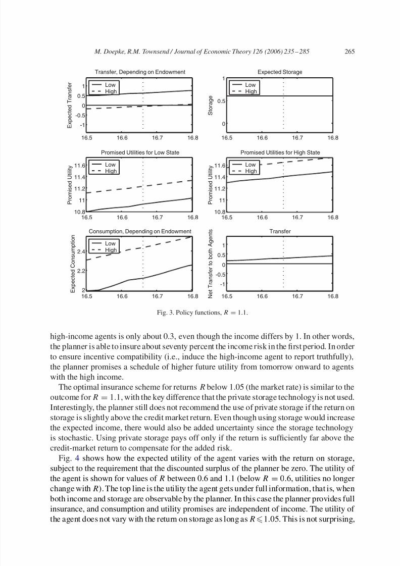
8/13/2019 Dopke Townsend (Dynamic Mechanism Design With Hidden Income and Hidden Actions)
http://slidepdf.com/reader/full/dopke-townsend-dynamic-mechanism-design-with-hidden-income-and-hidden-actions 31/51
M. Doepke, R.M. Townsend / Journal of Economic Theory 126 (2006) 235 – 285 265
16.5 16.6 16.7 16.8
-1
-0.5
0
0.5
1
-1
-0.5
0
0.5
1
Transfer, Depending on Endowment
E x p e c
t e d T r a n s
f e r
LowHigh
16.5 16.6 16.7 16.8
0
0.5
1Expected Storage
S t o r a g e
LowHigh
16.5 16.6 16.7 16.810.8
11
11.2
11.4
11.6
Promised Utilities for Low State
P r o m
i s e
d U t i l i t y Low
High
16.5 16.6 16.7 16.810.8
11
11.2
11.4
11.6
Promised Utilities for High State
P r o m
i s e
d U t i l i t y Low
High
16.5 16.6 16.7 16.8
2
2.2
2.4
Consumption, Depending on Endowment
E x p e c
t e d C o n s u m p
t i o n
LowHigh
16.5 16.6 16.7 16.8
Transfer
N
e t T r a n s
f e r
t o b o
t h A g e n
t s
Fig. 3. Policy functions, R = 1.1.
high-income agents is only about 0.3, even though the income differs by 1. In other words,the planner is able to insure about seventy percent the income risk in the rst period. In orderto ensure incentive compatibility (i.e., induce the high-income agent to report truthfully),the planner promises a schedule of higher future utility from tomorrow onward to agentswith the high income.
The optimal insurance scheme for returns R below 1.05 (the market rate) is similar to the
outcome for R = 1.1, with the key difference that the private storage technology is not used.Interestingly, the planner still does not recommend the use of private storage if the return onstorage is slightly above the credit market return. Even though using storage would increasethe expected income, there would also be added uncertainty since the storage technologyis stochastic. Using private storage pays off only if the return is sufciently far above thecredit-market return to compensate for the added risk.
Fig. 4 shows how the expected utility of the agent varies with the return on storage,subject to the requirement that the discounted surplus of the planner be zero. The utility of the agent is shown for values of R between 0.6 and 1.1 (below R = 0.6, utilities no longerchange with R ). The top line is the utility the agent gets under full information, that is, whenboth income and storage are observable by the planner. In this case the planner provides fullinsurance, and consumption and utility promises are independent of income. The utility of the agent does not vary with the return on storage as long as R 1.05. This is not surprising,

8/13/2019 Dopke Townsend (Dynamic Mechanism Design With Hidden Income and Hidden Actions)
http://slidepdf.com/reader/full/dopke-townsend-dynamic-mechanism-design-with-hidden-income-and-hidden-actions 32/51
266 M. Doepke, R.M. Townsend / Journal of Economic Theory 126 (2006) 235– 285
0.6 0.65 0.7 0.75 0.8 0.85 0.9 0.95 1 1.05 1.116.63
16.635
16.64
16.645
16.65
16.655
16.66
16.665
16.67Utility of Agent at Zero Surplus
U t i l i t y
R (Return on Storage)
First BestSecond BestCredit MarketAutarky
Fig. 4. Utility of the agent with full information, private information, credit-market access, and autarky.
since 1.05 is the risk-free interest rate. As long as the return on storage does not exceedthe credit-market return, storage is never used. When R exceeds 1.05, the Pareto frontierexpands and the utility of the agent increases dramatically. In effect, when R > 1.05 anarbitrage opportunity arises which is only limited by the upper bound on storage.
The lower line shows the utility of the agent under autarky. When the return on storageis sufciently high (above about 0.91, still a relatively dismal return) the agent uses storageto self-insure against the income shocks. Since under autarky storage is the only insurance
for the agent, utility increases with the return on storage.Thesolid line shows theutility of theagent under optimal incentive-constrained insurance
with hidden income and hidden actions. Once the return on storage exceeds some criticalvalue (about 0.7), the utility of the agent decreases with the return on storage, instead of increasingas it does under autarky.As long as theplanner neverrecommends positiveprivatestorage, a higher return on storage has no positive effects. On the contrary, it becomes harderto satisfy the obedience constraints which require that the agent does not prefer a positivestorage level when the planner recommends zero storage. Raising the return on storageshrinks the set of feasible allocations, and the utility of the agent falls. Hence, the propertiesof the storage technology inuence the optimal insurance contract even if private storage isnever used in equilibrium.
The dotted line represents the utility of an agent who has access to a perfect creditmarket under the same conditions as the planner. The agent can also use the private storage

8/13/2019 Dopke Townsend (Dynamic Mechanism Design With Hidden Income and Hidden Actions)
http://slidepdf.com/reader/full/dopke-townsend-dynamic-mechanism-design-with-hidden-income-and-hidden-actions 33/51
M. Doepke, R.M. Townsend / Journal of Economic Theory 126 (2006) 235 – 285 267
technology in addition to borrowing and lending in thecreditmarket. This utility is computedby solving for the optimal saving and borrowing decisions explicitly, i.e., no nite grids onconsumption or assets are imposed. As long as the return on storage does not exceed thecredit market interest rate, once again zero storage is optimal, and the utility is independentof the return on storage. When the return on storage exceeds the interest rate, the agent maygain by using the storage technology in addition to smoothing income in the credit market.
We know that, in principle, the information-constrained solution should be no worse thatwhat the agent can achieve independently when given access to an outside credit market,since any borrowing-and-lending plan is incentive compatible. In other words, the optimalinsurance scheme can reproduce anything that can be achieved in the credit market, so thatthe credit-market solution should provide a lower bound on the information-constrainedsolution. In Fig. 4, theoptimal constrained solution does dipbelowthecredit-market solutionfor a small range of R , which can be attributed to the nite grids used to compute theinformation-constrained regime. Even so, the gure provides a measure of the accuracy of our code, as the difference between the solution and the lower bound is very small.
Thus, within the bounds of approximation our computations bear out the prediction byCole and Kocherlakota [5] that the credit-market utility should equal the optimal-insuranceutility at the point where the interest rate and return on storage are equal, despite the factthat our storage technology is stochastic. For returns sufciently below R = 1.05, optimalinformation-constrained insurance does signicantly better than credit-market access. ForR < 1.05, the utility of the agent increases with R under both regimes, but the information-constrained solution once again dominates for sufciently high returns.
In sum, Fig. 4 shows that if the return on private storage is sufciently different fromthe outside interest rate, the agent does signicantly better with optimal insurance thanwith borrowing and lending. What matters here is the ability of the agent to circumventthe insurance scheme offered by the planner. The planner provides incentives for truthfulreporting by exploiting differences in the intertemporal rate of substitution between agentswith high- and low-income realizations. When the return on storage is close to the credit-market interest rate, agents have the possibility of smoothing income on their own, sothat differences in rates of substitution are small. Consequently, little additional insurancecan be offered. When there is a large difference between return on storage and interestrate, however, it is costly for agents to deviate from the recommended storage scheme (no
storage at low returns, maximum storage at high returns). The planner can use the resultingdifferences in rates of substitution to provide incentives for truthful reporting, which resultsin more insurance . 13
13 The exact gain from optimal insurance depends on the return on storage. At low returns, the quantitativegains relative to credit-market access are small. The maximum utility differential is equivalent to a permanentincrease in consumption of slightly above one-twentieth of one percent. If the return to storage is so low that thestorage technology is never used, self-insurance in a credit market achieves 95 percent of the utility gain of optimalinsurance relative to autarky. The relative gains from optimal insurance are higher when storage is actually used.
At the maximum return of R = 1 .1, the credit-market solution yields only 65 percent of the utility gain relativeto autarky that can be attained by optimal insurance. These numbers, of course, are particular to our example.Generally, the absolute gains achieved by optimal insurance increase with the amount of risk inherent in incomerealizations and the agent’s degree of risk aversion.

8/13/2019 Dopke Townsend (Dynamic Mechanism Design With Hidden Income and Hidden Actions)
http://slidepdf.com/reader/full/dopke-townsend-dynamic-mechanism-design-with-hidden-income-and-hidden-actions 34/51
268 M. Doepke, R.M. Townsend / Journal of Economic Theory 126 (2006) 235– 285
The optimal allocations in this application are computed subject to two types of incentiveconstraints: obedience constraints force the agent to take the right action, and truth-tellingconstraints ensure that the agent reports the actual income. What happens if only one typeof constraint is introduced? If we remove the truth-telling constraints (i.e., we assume thatthe actual income can be observed by the planner) and assume that the return on storagedoes not exceed the credit-market return, the situation is simple: The planner can providefull insurance against income shocks. In this case the obedience constraints are not bindingsince the optimal storage level is zero, which is also what the agent prefers if income shocksare fully insured. Conversely, if only the obedience constraints are removed, as if storagecould be observed, full insurance cannot be achieved. The outcome is essentially the sameas in the situation where storage is hidden, but the storage technology has zero gross return.The utilities are as in Fig. 4 for R = 0.6.
7.2. Unobserved effort with hidden productivity and training
We now present another example to put our methods for computing the double-actionenvironment in Section 6 to work. Since in this environment there are a number of differenttypes of incentive constraints, we chose an extension of a relatively standard unobserved-effort economy to demonstrate how these different constraints interact. The state e in thiseconomy will be labeled as “productivity.” The rst action a 1 is interpreted as effort, anda 1 together with the state e jointly determine the probability distribution over output y.The second unobserved action a2 is interpreted as “training” or “skill acquisition,” and
determines the probability distribution over future productivity e .The agent enters the period with a productivity state e that can be either high or low(normalized to e = 1 and 0). The rst unobserved action (“effort”) a1 can also be eitherhigh or low ( a 1 = 1 or a 1 = 0). Next, (observable) income y is realized. Once again just twovalues are possible, y = 10 or y = 1. Table 1 shows the probability distribution over outputas a function of e and a1 . Notice that when effort a1 is low, the probability distribution overoutput does not depend on productivity e. A productive agent, on the other hand, gets amuch larger increase in the probability of getting high output by exerting high effort than anunproductive agent. After output is realized, the planner hands out a transfer . The secondunobserved action a2 (“training”) takes place at the end of the period, and can take the two
values a2 = 1 and a2 = 0. For a worker who does the training ( a 2 = 1), the probabilityof being productive in the next period ( e = 1) is 0.9, while without training ( a 2 = 0) theprobability is only 0.1. The utility function of the agent is given by
u(c, a 1 , a 2) =√ c − 1a 1 − 2a 2 ,
where 1 = 1 and 2 = 0 .2. Thus, preferences are separable in consumption and the twoeffort choices (this simplies interpreting the results; our computational method does notrequire separability assumptions).
In summary, we are considering a fairly standard unobserved effort model, which is en-
richedbythesecondunobservedaction“training”andtheunobservedstate“productivity.”14
14 Other interpretations of this environment are possible, such as two-stage crop production where the rst actionis “harvest” and the second action is “sowing” for the next season.

8/13/2019 Dopke Townsend (Dynamic Mechanism Design With Hidden Income and Hidden Actions)
http://slidepdf.com/reader/full/dopke-townsend-dynamic-mechanism-design-with-hidden-income-and-hidden-actions 35/51
M. Doepke, R.M. Townsend / Journal of Economic Theory 126 (2006) 235 – 285 269
Table 1Probability distribution over output y
e
= 0, a1
= 0 e
= 0, a1
= 1 e
= 1, a1
= 0 e
= 1, a1
= 1
P (y = 1) 0.9 0.8 0.9 0.1P (y = 10) 0.1 0.2 0.1 0.9
To map out how the optimal solution of the planning problem is affected by the differentincentive problems, we computed solutions under different assumptions on observability,ranging from full information to the case where e, a1, and a2 are all unobserved. Forsimplicity, a two-period model was computed, and we used Program 4 for all computations(while omitting some of the incentive constraints when some or all of e, a1, and a2 are
observable) .15
In the rst period, each productivity state occurs with probability 0.5.As a reference, Fig. 5 shows the optimal policy functions in the rst period under fullinformation ( e , a1 , and a2 all observed) as a function of the reservation W 0 utility of theagent. Displayed are the two action choices in the rst period as a function of the state(productive or unproductive), consumption as a function of output (separate graphs foreach productivity state), and the utility promises conditional on tomorrow’s productivity(again, there are separate graphs for each productivity state in the rst period). Giventhe effect of the effort a1 on output y, it turns out to be optimal to require high effortonly from productive agents. Since utility is concave in consumption, consumption is notconditional on type or output. At rst sight, it may seem surprising that the future utility
promise is lower for the high state than the low state. The reason is that in the second periodconsumption is independent of type or output once again, whereas only the productiveagent will be required to put in high effort, which explains the lower promise for productiveagents.
We now start to move towards the information-constrained solution. Fig. 6 shows theoutcome if the state e (productivity) is unobserved in both periods, but the two actionscontinue to be public information. The planner now needs to provide incentives to theagents to reveal the true state. As the upper-left panel shows, for most of the range of initialutility promises only the productive agent is required to exert high effort in the rst period.Since effort is costly in terms of utility, the productive agent is compensated for this effort
with higherconsumption, lower required training, and higher futureutility promises. Notice,however, that consumption does not depend on realized output: since effort is observable,the planner does not need to provide incentives to exert high effort once the productivitystate e has been revealed.
Over most of the range of initial utility promises, unlike in the full-information solutionthe utility promises for period 2 turn out not to depend on the future state e . In the full
15 We used the same technology as described in footnote 12. The grid for the transfer had 50 values inboth periods, and the grid for utility promises had 30 elements per state in income (resulting in 900 possiblecombinations, not all of which where feasible). Eighteen hundred programs had to be solved in period 2. In the
version with e, a1 , and a 2 all unobserved, each linear program had 200 variables and 12 constraints and took onaverage 0.007s to compute. In the rst (initial) period, each program had 99,602 variables and 3607 constraints,which resulted in an average computation time of 10.78s on average. The programs where some or all of e , a 1 ,and a2 are observed have fewer constraints and compute correspondingly faster.
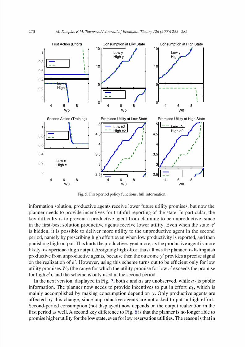
8/13/2019 Dopke Townsend (Dynamic Mechanism Design With Hidden Income and Hidden Actions)
http://slidepdf.com/reader/full/dopke-townsend-dynamic-mechanism-design-with-hidden-income-and-hidden-actions 36/51
270 M. Doepke, R.M. Townsend / Journal of Economic Theory 126 (2006) 235– 285
4 6 8
0
0.2
0.4
0.6
0.8
1
First Action (Effort)
W0
Low eHigh e
4 6 80
5
10
15Consumption at Low State
W0
Low yHigh y
4 6 80
5
10
15Consumption at High State
W0
Low yHigh y
4 6 8
0
0.2
0.4
0.6
0.8
1
Second Action (Training)
W0
Low eHigh e
4 6 82.5
3
3.5
4
4.5
5Promised Utility at Low State
W0
Low e2High e2
4 6 82.5
3
3.5
4
4.5
5Promised Utility at High State
W0
Low e2High e2
Fig. 5. First-period policy functions, full information.
information solution, productive agents receive lower future utility promises, but now theplanner needs to provide incentives for truthful reporting of the state. In particular, thekey difculty is to prevent a productive agent from claiming to be unproductive, sincein the rst-best solution productive agents receive lower utility. Even when the state eis hidden, it is possible to deliver more utility to the unproductive agent in the secondperiod, namely by prescribing high effort even when low productivity is reported, and then
punishing high output. This hurts the productive agent more, as the productive agent is morelikely to experience high output. Assigning high effort thus allows the planner to distinguishproductive from unproductive agents, because then the outcome y provides a precise signalon the realization of e . However, using this scheme turns out to be efcient only for lowutility promises W 0 (the range for which the utility promise for low e exceeds the promisefor high e ), and the scheme is only used in the second period.
In the next version, displayed in Fig. 7, both e and a1 are unobserved, while a2 is publicinformation. The planner now needs to provide incentives to put in effort a1, which ismainly accomplished by making consumption depend on y. Only productive agents areaffected by this change, since unproductive agents are not asked to put in high effort.Second-period consumption (not displayed) now depends on the output realization in therst period as well. A second key difference to Fig. 6 is that the planner is no longer able topromise higher utility for the low state, even for low reservation utilities.The reason is that in

8/13/2019 Dopke Townsend (Dynamic Mechanism Design With Hidden Income and Hidden Actions)
http://slidepdf.com/reader/full/dopke-townsend-dynamic-mechanism-design-with-hidden-income-and-hidden-actions 37/51
M. Doepke, R.M. Townsend / Journal of Economic Theory 126 (2006) 235 – 285 271
4 6 8
0
0.2
0.4
0.6
0.8
1
First Action (Effort)
W0
Low eHigh e
4 6 80
5
10
15Consumption at Low State
W0
Low yHigh y
4 6 80
5
10
15Consumption at High State
W0
Low yHigh y
4 6 8
0
0.2
0.4
0.6
0.8
1
Second Action (Training)
W0
Low eHigh e
4 6 81.5
2
2.5
3
3.5
4
4.5
5Promised Utility at Low State
W0
Low e2High e2
4 6 81.5
2
2.5
3
3.5
4
4.5
5Promised Utility at High State
W0
Low e2High e2
Fig. 6. First-period policy functions, e private information.
Fig. 6 the two productivity types could be distinguished only by assigning high effort a 1 = 1to both productive and unproductive agents in the second period. This is no longer incentivecompatible once effort a1 is unobserved as well. Thus, the combination of the two setsof incentive constraints forces the planner to offer identical utility promises to productiveand unproductive agents, which is not the case if either set of constraints is imposed in
isolation.To see how unobservability of training a2 affects the results, it is best to start with a
version where only a2 is unobserved, while e and a1 are public information. The results aredisplayed in Fig. 8. To provide incentives for training, the planner has to promise higherutility for the high future productivity state. Thus, in the region where positive training isassigned, the ranking of the utility promises across the two states is reversed relative tothe full-information solution. Finally, Fig. 9 shows the fully incentive-constrained versionwhere e, a1, and a2 are all unobserved. In the range where the recommended a2 is positive,the incentive constraints compel the planner to offer more utility promise for the futureproductive state. Even if the recommended a2 is zero, the planner has to offer at least asmuch utility at the productive state compared to the unproductive state to induce truthfulreporting of e (as in Fig. 7). Finally, consumption depends on y if a1 = 1 is recommended,so that high effort is incentive compatible.

8/13/2019 Dopke Townsend (Dynamic Mechanism Design With Hidden Income and Hidden Actions)
http://slidepdf.com/reader/full/dopke-townsend-dynamic-mechanism-design-with-hidden-income-and-hidden-actions 38/51
272 M. Doepke, R.M. Townsend / Journal of Economic Theory 126 (2006) 235– 285
4 6 8
0
0.2
0.4
0.6
0.8
1
First Action (Effort)
W0
Low eHigh e
4 6 80
5
10
15Consumption at Low State
W0
Low yHigh y
4 6 80
5
10
15Consumption at High State
W0
Low yHigh y
4 6 8
0
0.2
0.4
0.6
0.8
1
Second Action (Training)
W0
Low eHigh e
4 6 81.5
2
2.5
3
3.5
4
4.5
5Promised Utility at Low State
W0
Low e2High e2
4 6 81.5
2
2.5
3
3.5
4
4.5
5Promised Utility at High State
W0
Low e2High e2
Fig. 7. First-period policy functions, e, a1 private information.
To summarize, the results demonstrate that the features of the optimal contract are quitesensitive to the assumptions on exactly what can be observed by the planner. In Fig. 6, forexample, the planner wants to provide incentives for reporting the true endowment e. Forlow utility promises, this is accomplished by imposing high effort on the agent, becausethen the outcome y provides a precise signal on the realization of e. The insurance scheme
that deals with the hidden state e therefore relies on the action a1 being controlled by theplanner. If a1 is hidden as well, it not incentive-compatible for the agent to put in higheffort given that high output is punished subsequently, so the original insurance scheme isundercut. We conjecture that similar outcomes will arise in a variety of environments withmultiple hidden actions and states.
8. Conclusions
In this paper we show how general dynamic mechanism design problems with hiddenstates and hidden actions can be formulated in a way that is suitable for computation. Ourmethods can be applied to wide variety of models, including applications with incomeshocks or productivity shocks, and actions that could be interpreted as storage, investment,

8/13/2019 Dopke Townsend (Dynamic Mechanism Design With Hidden Income and Hidden Actions)
http://slidepdf.com/reader/full/dopke-townsend-dynamic-mechanism-design-with-hidden-income-and-hidden-actions 39/51
M. Doepke, R.M. Townsend / Journal of Economic Theory 126 (2006) 235 – 285 273
4 6 8
0
0.2
0.4
0.6
0.8
1
First Action (Effort)
W0
Low eHigh e
4 6 80
5
10
15Consumption at Low State
W0
Low yHigh y
4 6 80
5
10
15Consumption at High State
W0
Low yHigh y
4 6 8
0
0.2
0.4
0.6
0.8
1
Second Action (Training)
W0
Low eHigh e
4 6 8
1.5
2
2.5
3
3.5
4
4.5
5Promised Utility at Low State
W0
Low e2High e2
4 6 8
1.5
2
2.5
3
3.5
4
4.5
5Promised Utility at High State
W0
Low e2High e2
Fig. 8. First-period policy functions, a2 private information.
work effort, search effort, or training. We start from a general planning problem whichallows arbitrary message spaces, lotteries, and history dependence. The planning problem isreduced to a recursive version which imposes truth-telling and obedience and uses vectorsof utility promises as state variables. We also develop methods to reduce the number of constraints that need to be imposed when computing the optimal contract. The main ideaof these methods is to allow the planner to put structure on outcomes off the equilibrium
path. In particular, the planner chooses bounds that limit the utility the agent can get oncertain off-equilibrium branches that are reached if only if the agent misreports the state atthe beginning of the period. If there are multiple hidden actions within the period, we showthat multiple layers of such utility bounds can be used to implement the optimal contractefciently.
In an application to a model with hidden storage, we use our methods to examine howthe optimal insurance contract varies with the return of the private storage technology. Theonly existing results for this environment concern special cases where the return on storageis equal to the credit-market return faced by the planner (see [3,5,15] ). We observe thatin certain cases the utility of the agent can actually decrease as the return of the privatetechnology rises. This occurs when the return on public storage is sufciently high so thatin the constrained optimum only public storage is used. If now the return to the privatetechnology rises, it becomes more difcult for the planner to provide incentives for truth-

8/13/2019 Dopke Townsend (Dynamic Mechanism Design With Hidden Income and Hidden Actions)
http://slidepdf.com/reader/full/dopke-townsend-dynamic-mechanism-design-with-hidden-income-and-hidden-actions 40/51
274 M. Doepke, R.M. Townsend / Journal of Economic Theory 126 (2006) 235– 285
4 6 8
0
0.2
0.4
0.6
0.8
1
First Action (Effort)
W0
Low e1High e1
4 6 80
5
10
15Consumption at Low State e1
W0
Low yHigh y
4 6 80
5
10
15Consumption at High State e1
W0
Low yHigh y
4 6 8
0
0.2
0.4
0.6
0.8
1
Second Action (Training)
W0
Low e1High e1
4 6 81.5
2
2.5
3
3.5
4
4.5
5
Promised Utility at Low State e1
W0
Low e2High e2
4 6 81.5
2
2.5
3
3.5
4
4.5
5
Promised Utility at High State e1
W0
Low e2High e2
Fig. 9. First-period policy functions, e, a1 , and a2 private information.
telling and obedience, and consequently less insurance is possible. Thus the effect of a risingreturn of private investment on the agent’s utility in the constrained optimum is exactly theopposite of the effect that prevails under autarky, where a higher return raises utility.
In an application to a hidden effort model with productivity and training, we show howthe optimal contract varies depending on which events and actions can be observed bythe planner. In particular, we demonstrate how the different types of incentive constraints
interact, in the sense that the optimal outcome with multiple unobserved states and actionslooks very different from a combination of theoutcomes with each stateor actionunobservedindividually. The intuition for this nding is that insurance for a single information problemoften works by making outcomes contingent on an observed state or action, as in thestandard unobserved effort model where incentives are provided by making consumptiondepend on output, even though the agent is risk averse. If there are multiple unobservedstates and actions, the ability of the planner to impose such contingencies is undercut, andthe insurance cannot be provided in the standard form.
Acknowledgments
We are grateful to Harold Cole, Hugo Hopenhayn, Ken Judd, Marek Kapicka, LarsLjungqvist, Roger Myerson, Nicola Pavoni, Ned Prescott, Phil Reny, Tom Sargent, Steve

8/13/2019 Dopke Townsend (Dynamic Mechanism Design With Hidden Income and Hidden Actions)
http://slidepdf.com/reader/full/dopke-townsend-dynamic-mechanism-design-with-hidden-income-and-hidden-actions 41/51
M. Doepke, R.M. Townsend / Journal of Economic Theory 126 (2006) 235 – 285 275
Tadelis, Iván Werning, Ruilin Zhou, and seminar participants at Boston University, Chicago,Cleveland Fed, Gerzensee, IIES, MIT, Richmond Fed, Stanford, UCL, UCLA, UC SanDiego, the SED meeting in San José, and the SIEPR Conference on “Credit Market Fric-tions in the Macroeconomy” for helpful comments. We also thank the co-editor and twoanonymous referees for suggestions that substantially improved the paper. Matthias Doepkeacknowledges support by the NSF (Grant SES-0217051), and Robert Townsend was sup-ported by the NSF (Grant 318340) and the NICHD (Grant R01 HD027638).
Appendix A. Mathematical appendix
A.1. Proofs for all propositions
Proposition 1. There are reservation utilities W 0 R such that an optimal equilibriumexists .
Proof. We need to show that for some W 0 the set of equilibria is non-empty and compact,and that the objective function is continuous. To see that the set of equilibria is non-empty,notice that the planner can assign a zero transfer in all periods, and always send the samemessage. If the strategy of the agent is to choose the actions that are optimal under autarky,clearly all constraints are trivially satised for the corresponding initial utility W 0 . The setof all contracts that satisfy the probability-measure constraints is compact in the product
topology since and are probability measures on nite support. Since only equalities andweak inequalities are involved, it can be shown that constraints ( 3) and ( 4) dene a closedsubset of this set. Since closed subsets of compact sets are compact, the set of all feasiblecontracts is compact. We still need to show that the objective function of the planner iscontinuous. Notice that the product topology corresponds to pointwise convergence, i.e.,we need to show that for a sequence of contracts that converges pointwise, the surplus of the planner converges. This is easy to show since we assume that the discount factor of the planner is smaller than one, and that the set of transfers is bounded. Let n , n , be asequence of contracts that converges pointwise to , , and choose > 0. We have to showthat there is an N such that
|V ( n , n )
−V ( , )
| < . Since the transfer is bounded and
Q < 1, there is an T such that the discounted surplus of the planner from time T on issmaller than / 2. Thus we only have to make the difference for the rst T periods smallerthan / 2, which is the usual Euclidian nite-dimensional case.
Proposition 2 ( Revelation Principle ). For any message spaces M 1 and M 2 , any allocationthat is feasible in the general mechanism is also feasible in the truth-telling mechanism .
Proof (Outline ). Corresponding to any feasible allocation in the general setup there is a fea-sible contract that implements this allocation. Fix a feasible allocation and thecorrespondingcontract {, }. We will now dene an outcome function for the truth-telling mechanismthat implements the same allocation. To complete the proof, we then have to show that thisoutcome function satises constraints ( 6)–(8).
8/13/2019 Dopke Townsend (Dynamic Mechanism Design With Hidden Income and Hidden Actions)
http://slidepdf.com/reader/full/dopke-townsend-dynamic-mechanism-design-with-hidden-income-and-hidden-actions 42/51

8/13/2019 Dopke Townsend (Dynamic Mechanism Design With Hidden Income and Hidden Actions)
http://slidepdf.com/reader/full/dopke-townsend-dynamic-mechanism-design-with-hidden-income-and-hidden-actions 43/51
M. Doepke, R.M. Townsend / Journal of Economic Theory 126 (2006) 235 – 285 277
Proposition 4. For all w0 W and e0 E , and for any sk−1 and ek , there is an optimalcontract such that the remaining contract from s k−1 and ek on is an optimal contract for the auxiliary planning problem with e0
= ek and w0
= w(s k−1 , ).
Proof. We will rst construct from a contract which is optimal from time zero and anothercontract which is optimal starting at sk−1 and ek . We will then show by a contradictionargument that is an optimal contract from time zero as well.
We have shown earlier that an optimal contract exists. Let be an optimal contract fromtime zero, and k an optimal contract for e0 = ek and w0 = w(s k−1 , ) , with the elementsof vector w(s k−1 , ) dened in (12). Now construct a new contract that is equal to kfrom (ek , s k−1) on, and equals until time k and on all future branches other than ek , s k−1 .First, notice that by the way is constructed, we have w(s k−1 , )
= w(s k−1 , ), and since
equals k from (e k , s k−1) , fullls the reoptimization requirement of the proposition.We now claim that is also an optimal contract. To show this, we have to demonstratethat satises constraints ( 6)–(8), and that it maximizes the surplus of the planner subjectto these constraints. To start, notice that the constraints that are imposed if we compute anoptimal contract taking e0 = ek and w0 = w(s k−1 , ) as the starting point also constrainthe choices of the planner in the original program from (e k , s k−1) onward. By reoptimizingat (ek , s k−1) in period k as if the game were restarted, the planner clearly cannot lowerhis surplus since no additional constraints are imposed. Therefore the total surplus fromcontract cannot be lower than the surplus from . Since is assumed to be an optimalcontract, if satises ( 6)–(8), it must be optimal as well. Thus we only have to show that(6)–(8) are satised, or in other words, that reoptimizing at ek , s k−1 does not violate anyconstraints of the original problem.
The probability constraints ( 6) are satised by contract , since the reoptimized contractis subject to the same probability constraints as the original contract. The promise-keepingconstraint ( 7) is satised since the new contract delivers the same on-path utilities by con-struction. We still have to show that the incentive constraints (8) are satised. We will do thisby contradiction. Suppose that ( 8) is not satised by contract . Then there is a deviation
such that for some s l , e l+1:
∞t =l+1
t
H t p(h t | , , s l , e l+1)u(e t + t − a (h t −1 , e t , t , a t ))
>∞
t =l+1
t
S t p(s t | , s l , e l+1)u(e t + t −a t ) . (44)
Consider rst the case l + 1 k. On any branch that starts at or after time k, contract is entirely identical to either or k . But then (44) implies that either or k violatesincentive-compatibility ( 8), a contradiction. Consider now the case l + 1 < k . Here thecontradiction is not immediate, since the remaining contract is a mixture of and k . Usingw(e k , s k−1 , ) to denote the continuation utility of the agent from time k on under the

8/13/2019 Dopke Townsend (Dynamic Mechanism Design With Hidden Income and Hidden Actions)
http://slidepdf.com/reader/full/dopke-townsend-dynamic-mechanism-design-with-hidden-income-and-hidden-actions 44/51
278 M. Doepke, R.M. Townsend / Journal of Economic Theory 126 (2006) 235– 285
deviation strategy, we can rewrite ( 44) ask−1
t =l+1
t
H t p(h t
|, , s l , e l
+1)u(e t
+t
−a (h t −1 , e t , t , a t ))
+ k
E,s k−1
p(e k , s k−1| , , s l , e l+1)w(e k , s k−1 , )
>k−1
t =l+1
t
S t p(s t | , s l , e l+1)u(e t + t −a t )
+ k
E,s k−1
p(e k , s k−1| , s l , e l+1)w(e k , s k−1). (45)
Notice that for sk
−1
that are reached with positive probability under the deviation we have:w(e k , s k−1 , ) w(e k , (s k−1)), (46)
where (s k ) is the history as seen by the planner (reported incomes, delivered transfers,and recommended actions) under the deviation strategy. Otherwise, either or k wouldviolate incentive constraints. To see why, assume that ek , s k−1 is a branch after which isidentical to . If we had w(e k , s k−1 , ) > w(e k , (s k−1)) , an agent under contract whoreached history (s k−1) could gain by following the deviation strategy afterwards. Thiscannot be the case since is assumed to be an optimal contract, and therefore deviationsare never protable. Using (46) in (45) gives
k−1
t =l+1
t
H t p(h t | , , s l , e l+1)u(e t + t − a (h t −1 , e t , t , a t ))
+ k
E,s k−1
p(e k , s k−1| , , s l , e l+1)w(e k , (s k−1))
>k−1
t =l+1
t
S t p(s t | , s l , e l+1)u(e t + t −a t )
+k
E,s k−1
p(e k , s k−1
|, s l , e l
+1)w(e k , s k−1). (47)
The outcome function enters ( 47) only up to time k − 1. Since up to time k − 1 theoutcome function is identical to , and since by construction of continuation utilitiesat time k are the same under and , we can rewrite ( 47) as
k−1
t =l+1
t
H t p(h t | , , s l , e l+1)u(e t + t − a (h t −1 , e t , t , a t ))
+ k
E,s k−1
p(e k , s k−1| , , s l , e l+1)w(e k , (s k−1))
>k−1
t =l+1
t
S t p(s t | , s l , e l+1)u(e t + t −a t )
8/13/2019 Dopke Townsend (Dynamic Mechanism Design With Hidden Income and Hidden Actions)
http://slidepdf.com/reader/full/dopke-townsend-dynamic-mechanism-design-with-hidden-income-and-hidden-actions 45/51
M. Doepke, R.M. Townsend / Journal of Economic Theory 126 (2006) 235 – 285 279
+ k
E,s k−1
p(e k , s k−1| , s l , e l+1)w(e k , s k−1). (48)
But now the left-hand side of ( 48) is the utility that the agent gets under plan fromfollowing the deviation strategy until time k and following the recommendations of theplanner afterwards. Thus ( 48) contradicts the incentive compatibility of . We obtain acontradiction, thus actually satises ( 8). This shows that plan is within the constraintsof the original problem. Since yields at least as much surplus as and is an optimalcontract, must be optimal as well.
Proposition 5. Programs 1 and 2 are equivalent .
Proof. We want to show that constraints ( 28) and ( 29) in Program 2 place the same restric-tions on the outcome function (·) as the truth-telling constraints (23) of Program 1. Let usrst assume we have found a lottery ( , a, w |w , e) that satises the truth telling constraint(23) of Program 1 for all ˆe and : T × S → A. We have to show that there exist utilitybounds v( ˆe,e, , a) such that the same lottery satises ( 28) and (29) in Program 2. For each
ˆe , , and a , dene v( ˆe,e, , a) as the maximum of the left-hand side of ( 28) over all ˆa :
v( ˆe,e, , a)
≡ maxˆa W
( , a, w |w , e) u( ˆe + − ˆa) + E(e |ˆa)w (e ) . (49)
Then clearly ( 28) is satised, since the left-hand side of ( 28) runs over ˆa . Now for each and a , dene (̂·) by setting (̂ , a) equal to the ˆa that maximizes the left-hand side of (28):
(̂ , a)
≡arg max ˆaW
( , a, w |w , e) u( ˆe+ −ˆa) + E(e |ˆa)w (e ) . (50)
Since ( , a, w |w , e) satises ( 23) for any function (·) by assumption, we have for ourparticular (̂·):
T,A, W
( , a, w |w , e) u( ˆe+ −ˆ( ,a)) + E(e |ˆ( , a))w (e ) w( ˆe). (51)
By the way we chose (̂·) and the v(·), we have from (28):
W
( , a, w |w , e) u( ˆe + − (̂ ,a)) + E(e | (̂ , a))w (e )
= v( ˆe,e, ,a). (52)
Substituting the left-hand side into (51), we get
T ,Av( ˆe,e, , a) w( ˆe). (53)
which is ( 29).

8/13/2019 Dopke Townsend (Dynamic Mechanism Design With Hidden Income and Hidden Actions)
http://slidepdf.com/reader/full/dopke-townsend-dynamic-mechanism-design-with-hidden-income-and-hidden-actions 46/51
280 M. Doepke, R.M. Townsend / Journal of Economic Theory 126 (2006) 235– 285
Conversely, suppose we have found a lottery ( , a, w |w , e) that satises ( 28) and ( 29)in Program 2 for some choice of v( ˆe,e, , a) . By (28), we have then for any ˆe and ˆa andhence any
: T
×S
→ A :
W
( , a, w |w , e) u( ˆe + − ( ,a)) + E(e | ( , a))w (e )
v( ˆe,e, ,a). (54)
Substituting the left-hand side of ( 54) into the assumed (29)forthe v( ˆe,e, , a) , we maintainthe inequality:
T,A, W
( , a, w |w , e) u( ˆe+ − ( ,a)) + E(e | ( , a))w (e ) w( ˆe). (55)
But this is ( 23) in Program 1. Therefore the sets of constraints are equivalent, which provesthat Programs 1 and 2 are equivalent.
Proposition 6. Programs 3 and 4 are equivalent .
Proof. We want to show that constraints ( 38)–(41) in Program 4 place the same restrictionson the outcome function (·) as constraints ( 34) and ( 36) of Program 3. Let us rst assumewe have found a lottery (a 1 , y, , a 2 , w |w , e) that satises constraints ( 34) and (36) of Program 3 for all
ˆe, 1 , and 2 . We have to show that there exist utility bounds v(
ˆe,e, , a)
such that the same lottery satises ( 39)–(41) in Program 4. For each ˆe , a1 , ˆa 1, y , , and a2dene v2( ˆe, a 1 , ˆa 1 , y, , a 2) as the maximum of the left-hand side of ( 41) over all ˆa 2:
v2( ˆe, a 1 , ˆa 1 , y, , a 2)
≡ maxˆa2 W
(a 1 , y, , a 2 , w |w , e)f (y |ˆe, ˆa 1)f (y |e, a 1)
× u( ˆe, ˆa 1 , y, , ˆa 2) + Eg(e |ˆe, ˆa 1 , y, , ˆa 2)w (e ) . (56)
This choice guarantees that (38)and(41) are satised. Next, for all ˆe and a 1 , dene v1( ˆe, a 1)as the maximum over the left-hand side of ( 40):
v1( ˆe, a 1) ≡ maxˆa1 Y,T,A 2
v2( ˆe, a 1 , ˆa 1 , y, , a 2) . (57)
This choice guarantees that (40) is satised. Finally, ( 36), (40), and ( 41) jointly imply that(39) is satised (if itwereviolated, we could construct a deviation strategy thatviolates ( 36)).
Conversely, suppose we have found a lottery (a 1 , y, , a 2 , w |w , e) that satises ( 38)–
(41) in Program 4 for some choice of utility bounds. Because of ( 41), we have for any 2:
ˆe, a 1 , ˆa 1 , y, , a 2 ,W
(a 1 , y, , a 2 , w |w , e)f (y |ˆe, ˆa 1)f (y |e, a 1)

8/13/2019 Dopke Townsend (Dynamic Mechanism Design With Hidden Income and Hidden Actions)
http://slidepdf.com/reader/full/dopke-townsend-dynamic-mechanism-design-with-hidden-income-and-hidden-actions 47/51
M. Doepke, R.M. Townsend / Journal of Economic Theory 126 (2006) 235 – 285 281
× u( ˆe, ˆa 1 , y, , 2(a 1 , y, , a 2))
+ E
g(e
|ˆe,
ˆa 1 , y, , 2(a 1 , y, , a 2))w (e )
v2( ˆe, a 1 , ˆa 1 , y, , a 2). (58)
Plugging the left-hand side of this equation into ( 38) for the v2( ˆe, a 1 , ˆa 1 , y, , a 2) maintainsthe inequality, and therefore gives (34). We also have for any given 1 and 2:
ˆe, a 1 , y, , a 2 ,W
(a 1 , y, , a 2 , w |w , e)f (y |ˆe, 1(a 1))
f (y |e, a 1)
× u( ˆe, 1(a 1),y, , 2(a 1 , y, , a 2))
+ Eg(e
|ˆe, 1(a 1),y, , 2(a 1 , y, , a 2))w (e )
v2( ˆe, a 1 , 1(a 1),y, , a 2). (59)
Substituting the left-hand side of ( 40) for the given 1 into (39) gives
ˆe = e,A1 ,Y,T,A 2
v2( ˆe, a 1 , a 1 , y, , a 2) w( ˆe). (60)
Now we can replace the v2( ˆe, a 1 , a 1 , y, , a 2) in this equation by the left-hand side of ( 59)while maintaining the inequality:
ˆe
= e,
A1 ,Y,T,A 2 ,W
(a 1 , y, , a 2 , w
|w , e)
f (y |ˆe, 1(a 1))
f (y |e, a 1)
× u( ˆe, 1(a 1),y, , 2(a 1 , y, , a 2))
+ Eg(e |ˆe, 1(a 1),y, , 2(a 1 , y, , a 2))w (e ) w( ˆe), (61)
But this is ( 36) in Program 3 for our particular choice of 1 and 2. Since the choiceof 1 and 2 was arbitrary, (36) is satised, which shows that Programs 1 and 2 areequivalent.
A.2. Computing the value set
Our analysis was based on the assumption that the set W of feasible utility vectors isknown in advance. In practice, W is not known and needs to becomputed alongside the valuefunction V (w , e) . W can be computed with the dynamic-programming methods describedin detail in Abreu, Pierce, and Stachetti [2], henceforth APS. An outline of the methodfollows.
We start by dening an operator B that maps nonempty compact subsets of R#E intononempty compact subsets of R#E . Let W be a nonempty compact subset of R #E . ThenB( W ) is dened as follows:
Denition A.1. A utility vector w B( W ) if there exist probabilities ( , a |w , e) andfuture utilities w (w , e, , a) W such that ( 14)–(17) hold.
8/13/2019 Dopke Townsend (Dynamic Mechanism Design With Hidden Income and Hidden Actions)
http://slidepdf.com/reader/full/dopke-townsend-dynamic-mechanism-design-with-hidden-income-and-hidden-actions 48/51
282 M. Doepke, R.M. Townsend / Journal of Economic Theory 126 (2006) 235– 285
The key point is that utility promises are chosen from the set W instead of the true valueset W . Intuitively, B( W ) consists of all utility vectors w that are feasible today (observingall incentive constraints), given that utility vectors from tomorrow onward are drawn fromthe set W . The fact that B maps compact set into compact sets follows from the fact thatall constraints are linear and involve only weak inequalities. Clearly, the true set of feasibleutility vectors W satises W = B( W ) , thus W is a xed point of B . The computationalapproach described in APS consists of using B to dene a shrinking sequence of sets thatconverges to W .
To do this, we need to start with a set W 0 that is known to be larger than W a priori. Inour case, this is easy to do, since consumption is bounded and therefore lifetime utility isbounded above and below. We can choose W 0 as an interval in R#E from a lower boundthat is lower than the utility from receiving the lowest consumption forever to a numberthat exceeds utility from consuming the highest consumption forever. We can now dene asequence of sets W n by dening W n+1 as W n+1 = B(W n ) . We have the following results:
Proposition A.1.
• The sequence W n is shrinking , i.e. , for any n , W n+1 is a subset of Wn .
• For all n , W is a subset of W n .
• The sequence W n converges to a limit W̄ , and W is a subset of W̄ .
Proof. To see that W n is shrinking, we only need to show that W 1 is a subset of W 0. Since
W 0 is an interval, it sufces to show that the upper bound of W 1 is lower than the upperbound of W 0 , and that the lower bound of W 1 is higher than the lower bound of W 0 . Theupper bound of W 1 is reached by assigning maximum consumption in the rst period andthe maximum utility vector in W 0 from the second period onward. But the maximum utilityvector W0 by construction corresponds to consuming more than maximum consumptionevery period, and since utility is discounted, the highest utility vector in W1 therefore issmaller than the highest utility vector in W 0 .
To see that W is a subset of all W n , notice that by the denition of B , if C is a subset of D, B( C ) is a subset of B(D) . Since W is a subset of W 0 and W = B( W ) , we have that Wis a subset of W 1
= B( W 0) , and correspondingly for all the other elements.
Finally, Wn has to converge to a nonempty limit since it is a decreasing sequence of compact sets, and the nonempty set W is a subset of all elements of the sequence.
Up to this point, we know that W n converges to W̄ and that W is a subset of W̄ . What wewant to show is that W̄ and W are actually identical. What we still need to show, therefore,is that W̄ is also a subset of W .
Proposition A.2. The limit set W̄ is a subset of the true value set W .
Proof. The outline of the proof is as follows. To show that an element w of
¯W is in W ,
we have to nd ( t , a t |et , s t −1) that satisfy constraints ( 6), (8), and ( 10) for w. These( t , a t |et , s t −1) can be constructed period by period from the that are implicit in the
denition of the operator B . Notice that in each period continuation utilities are drawn from

8/13/2019 Dopke Townsend (Dynamic Mechanism Design With Hidden Income and Hidden Actions)
http://slidepdf.com/reader/full/dopke-townsend-dynamic-mechanism-design-with-hidden-income-and-hidden-actions 49/51

8/13/2019 Dopke Townsend (Dynamic Mechanism Design With Hidden Income and Hidden Actions)
http://slidepdf.com/reader/full/dopke-townsend-dynamic-mechanism-design-with-hidden-income-and-hidden-actions 50/51
284 M. Doepke, R.M. Townsend / Journal of Economic Theory 126 (2006) 235– 285
value set W as the set of possible utility promises, the resulting linear program would havean innite number of variables (though still a nite number of constraints), since probabilityweight could be put on any of the generally innitely many members of W . We can think of our nite linear programs as versions of the general innite-dimensional linear programsunder additional restrictions,namely that zero probability be assigned to all but a given niteset of future utility promises. Hernández-Lerma and Lasserre [12] provide conditions underwhich the values of a sequence of such restricted linear programs converge to the value of thetrue innite-dimensional program (see their Proposition 2.2 and Theorem 3.2). Translatedinto our application, if Wk is an increasing sequence of nite approximations of W suchthat Wk W , the key condition is that ∞k=0W k is dense in W . It may seem that theseresults should apply easily to our environment, since W is a subset of an interval in R #E .However, notice that the W k cannot be chosen directly, but would have to be generated as a
xed point of the BD
operator for each k, so without additional assumptions the propertiesof W k cannot be directly inferred.As a practical matter, it is sometimes possible to judge the quality of approximations if
there are special cases with known solutions. The hidden storage application in Section 7.1provides such an example, since there are theoretical results that apply to the case when theplanner and the agent face the same credit-market return.
References
[1] A. Abraham, N. Pavoni, Efcient allocations with moral hazard and hidden borrowing and lending,Unpublished Manuscript, UCL and LBS, 2002.
[2] D.Abreu, D. Pearce, E. Stacchetti, Toward a theory of discounted repeated games with imperfect monitoring,Econometrica 58 (1990) 1041–1063.
[3] F. Allen, Repeated principal-agent relationships with lending and borrowing, Econ. Lett. 17 (1985) 27–31.[4] H.L. Cole, N.R. Kocherlakota, Dynamic games with hidden actions and hidden states, J. Econ. Theory 98
(2001) 114–126.[5] H.L. Cole, N.R. Kocherlakota, Efcient allocations with hidden income and hidden storage, Rev. Econ. Stud.
68 (2001) 523–542.[6] M. Doepke, R.M. Townsend, Dynamic mechanism design with hidden income and hidden actions: technical
appendix, UCLA Department of Economics Working Paper No. 819, 2002.[7] A. Fernandes, C. Phelan, A recursive formulation for repeated agency with history dependence, J. Econ.
Theory 91 (2000) 223–247.[8] D. Fudenberg, B. Holmstrom, P. Milgrom, Short-term contracts and long-term agency relationships, J. Econ.
Theory 51 (1990) 1–31.[9] E.J. Green, Lending and the smoothing of uninsurable income, in: E. Prescott, N. Wallace (Eds.), Contractual
Arrangements for Intertemporal Trade, University of Minnesota Press, Minneapolis, 1987, pp. 3–25.[10] M. Harris, R.M. Townsend,Allocation mechanisms for asymetrically informed agents, Manuscript presented
at the NBER-CME Conference Honoring Herb Simon, 1977.[11] M. Harris, R.M. Townsend, Resource allocation under asymmetric information, Econometrica 49 (1981)
33–64.[12] O. Hernández-Lerma, J.B. Lasserre, Approximation schemes for innite linear programs, SIAM J. Optim. 8
(1998) 973–988.[13] K.L. Judd, S. Yeltekin, J. Conklin, Computing supergame equilibria, Econometrica 71 (2003) 1239–1254.
[14] N.R. Kocherlakota, Figuring out the impact of hidden savings on optimal unemployment insurance, Rev.Econ. Dyn. 7 (2004) 541–554.[15] L. Ljungqvist, T.J. Sargent, Recursive macroeconomic theory, Manuscript for second ed., 2003.[16] R.B. Myerson, Incentive compatibility and the bargaining problem, Econometrica 47 (1979) 61–73.
8/13/2019 Dopke Townsend (Dynamic Mechanism Design With Hidden Income and Hidden Actions)
http://slidepdf.com/reader/full/dopke-townsend-dynamic-mechanism-design-with-hidden-income-and-hidden-actions 51/51
M. Doepke, R.M. Townsend / Journal of Economic Theory 126 (2006) 235 – 285 285
[17] R.B. Myerson, Optimal coordination mechanisms in generalized principal agent problems, J. Math. Econ.10 (1982) 67–81.
[18] R.B. Myerson, Multistage games with communication, Econometrica 54 (1986) 323–358.
[19] C. Phelan, Repeated moral hazard and one-sided commitment, J. Econ. Theory 66 (1995) 488–506.[20] C. Phelan, R.M. Townsend, Computing multi-period, information-constrained optima, Rev. Econ. Stud. 58
(1991) 853–881.[21] E.S. Prescott, Communication in models with private information: theory and computation, Geneva Papers
Risk Insurance Theory 28 (2003) 105–130.[22] S. Spear, S. Srivastava, On repeated moral hazard with discounting, Rev. Econ. Stud. 54 (1987) 599–618.[23] J. Thomas, T. Worrall, Income uctuations and asymmetric information: an example of a repeated principal-
agent problem, J. Econ. Theory 51 (1990) 367–390.[24] R.M. Townsend, Optimal contracts and competitive markets with costly state verication, J. Econ. Theory
21 (1979) 265–293.[25] R.M. Townsend, Optimal multiperiod contracts and the gain from enduring relationships under private
information, J. Polit. Economy 90 (1982) 1166–1186.
[26] R.M. Townsend, Information constrained insurance: the revelation principle extended, J. Monetary Econom.21 (1988) 411–450.
[27] C. Wang, Dynamic insurance with private information and balanced budgets, Rev. Econ. Stud. 62 (1995)577–595.
[28] I. Werning, Repeated moral hazard with unmonitored wealth: a recursive rst-order approach, UnpublishedManuscript, University of Chicago, 2001.


![Louisa Jane Townsend [249]townsend/tree/scrapbooks/249.pdfLouisa Jane Townsend [249] Transcription of a letter from John Henry Townsend [238] to Donald McLean concerning Louisa’s](https://static.fdocuments.in/doc/165x107/5ff3173b71622860d71c73dc/louisa-jane-townsend-249-townsendtreescrapbooks249pdf-louisa-jane-townsend.jpg)